L6: Short-time Fourier analysis and synthesisresearch.cs.tamu.edu/prism/lectures/sp/l6.pdf · L6: Short-time Fourier analysis and synthesis

Introduction to Speech Processing | Ricardo Gutierrez-Osuna | CSE@TAMU 1

L6: Short-time Fourier analysis and synthesis

• Overview

• Analysis: Fourier-transform view

• Analysis: filtering view

• Synthesis: filter bank summation (FBS) method

• Synthesis: overlap-add (OLA) method

• STFT magnitude

This lecture is based on chapter 7 of [Quatieri, 2002]


Overview

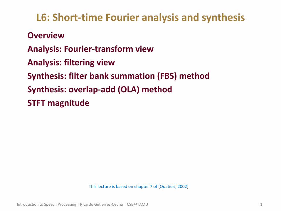
• Recap from previous lectures – Discrete time Fourier transform (DTFT)

• Taking the expression of the Fourier transform 𝑋 𝑗𝜔 = 𝑥(𝑡)𝑒−𝑗𝜔𝑡𝑑𝑡∞

−∞,

the DTFT can be derived by numerical integration

𝑋 𝑒𝑗𝜔 = 𝑥 𝑛 𝑒−𝑗𝜔 𝑛∞

−∞

– where 𝑥 𝑛 = 𝑥 𝑛𝑇𝑆 and 𝜔 = 2𝜋𝐹 𝐹𝑆

– Discrete Fourier transform (DFT)

• The DFT is obtained by “sampling” the DTFT at 𝑁 discrete frequencies 𝜔𝑘 = 2𝜋𝐹𝑠 𝑁 , which yields the transform

𝑋 𝑘 = 𝑥 𝑛 𝑒−𝑗2𝜋𝑁

𝑘𝑛𝑁−1

𝑛=0


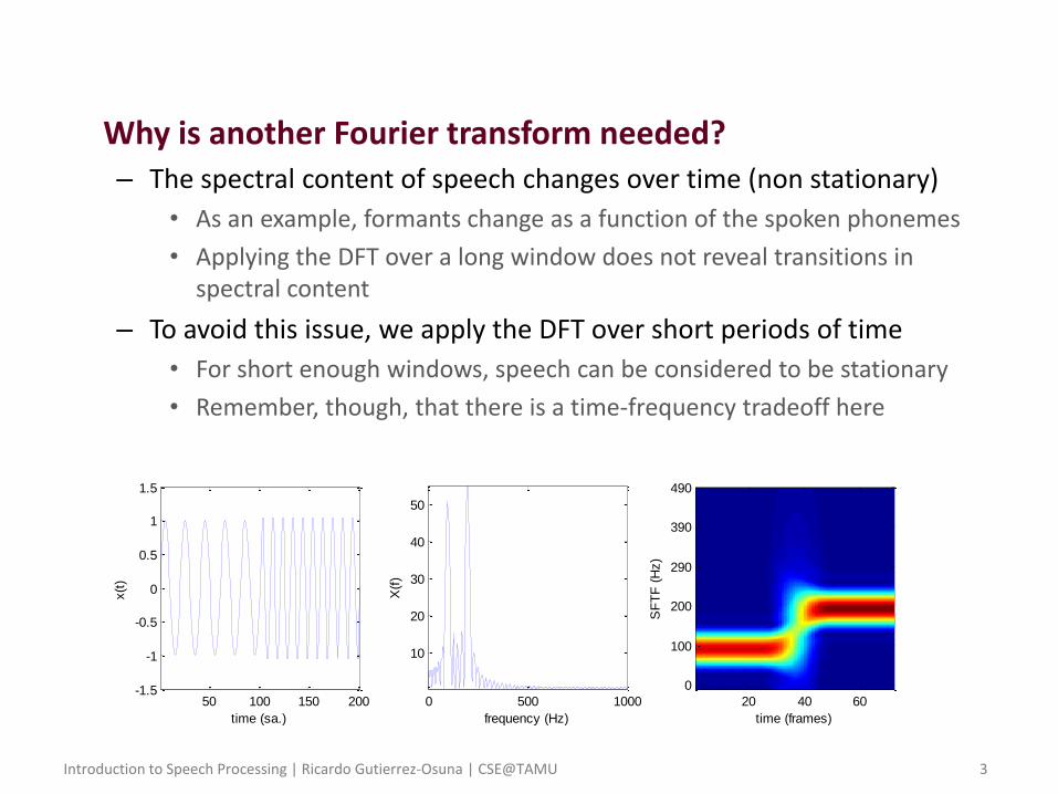
• Why is another Fourier transform needed? – The spectral content of speech changes over time (non stationary)

• As an example, formants change as a function of the spoken phonemes

• Applying the DFT over a long window does not reveal transitions in spectral content

– To avoid this issue, we apply the DFT over short periods of time

• For short enough windows, speech can be considered to be stationary

• Remember, though, that there is a time-frequency tradeoff here

50 100 150 200-1.5

-1

-0.5

0

0.5

1

1.5

time (sa.)

x(t

)

0 500 1000

10

20

30

40

50

frequency (Hz)

X(f

)

time (frames)

SF

TF

(H

z)

20 40 60

490

390

290

200

100

0


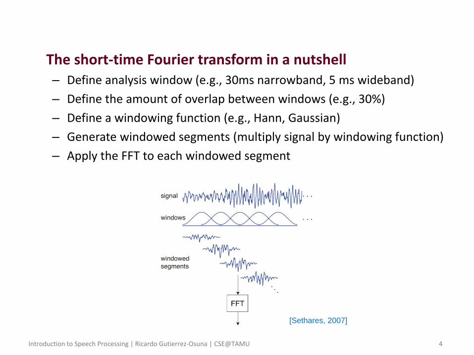
• The short-time Fourier transform in a nutshell – Define analysis window (e.g., 30ms narrowband, 5 ms wideband)

– Define the amount of overlap between windows (e.g., 30%)

– Define a windowing function (e.g., Hann, Gaussian)

– Generate windowed segments (multiply signal by windowing function)

– Apply the FFT to each windowed segment

[Sethares, 2007]


STFT: Fourier analysis view

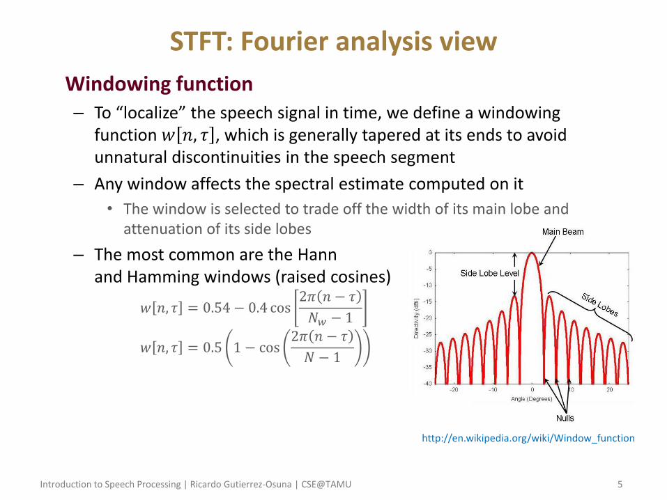
• Windowing function – To “localize” the speech signal in time, we define a windowing

function 𝑤 𝑛, 𝜏 , which is generally tapered at its ends to avoid unnatural discontinuities in the speech segment

– Any window affects the spectral estimate computed on it

• The window is selected to trade off the width of its main lobe and attenuation of its side lobes

– The most common are the Hann and Hamming windows (raised cosines)

𝑤 𝑛, 𝜏 = 0.54 − 0.4 cos2𝜋 𝑛 − 𝜏

𝑁𝑤 − 1

𝑤 𝑛, 𝜏 = 0.5 1 − cos2𝜋 𝑛 − 𝜏

𝑁 − 1

http://en.wikipedia.org/wiki/Window_function


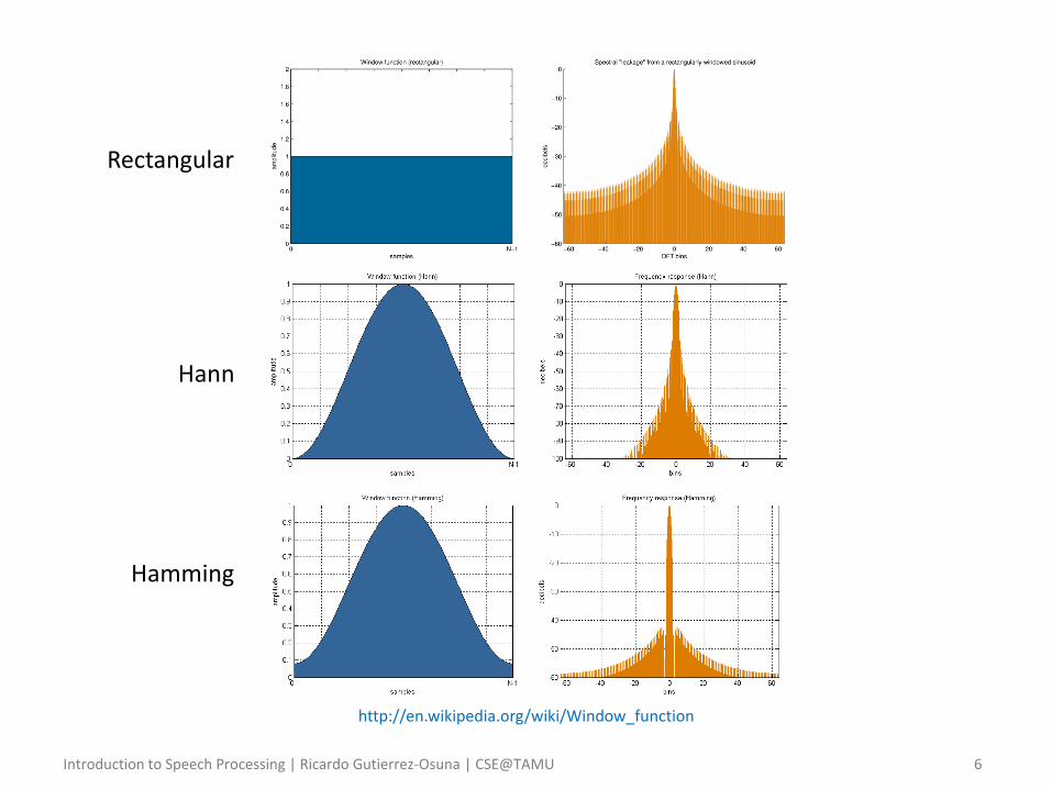
Rectangular

Hann

Hamming

http://en.wikipedia.org/wiki/Window_function


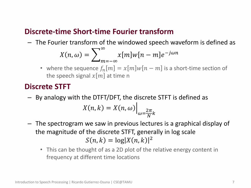
• Discrete-time Short-time Fourier transform – The Fourier transform of the windowed speech waveform is defined as

𝑋 𝑛, 𝜔 = 𝑥 𝑚 𝑤 𝑛 − 𝑚 𝑒−𝑗𝜔𝑛∞

𝑚=−∞

• where the sequence 𝑓𝑛 𝑚 = 𝑥 𝑚 𝑤 𝑛 − 𝑚 is a short-time section of the speech signal 𝑥 𝑚 at time n

• Discrete STFT – By analogy with the DTFT/DFT, the discrete STFT is defined as

𝑋 𝑛, 𝑘 = 𝑋 𝑛, 𝜔 𝜔=

2𝜋𝑁

𝑘

– The spectrogram we saw in previous lectures is a graphical display of the magnitude of the discrete STFT, generally in log scale

𝑆 𝑛, 𝑘 = log 𝑋 𝑛, 𝑘 2

• This can be thought of as a 2D plot of the relative energy content in frequency at different time locations


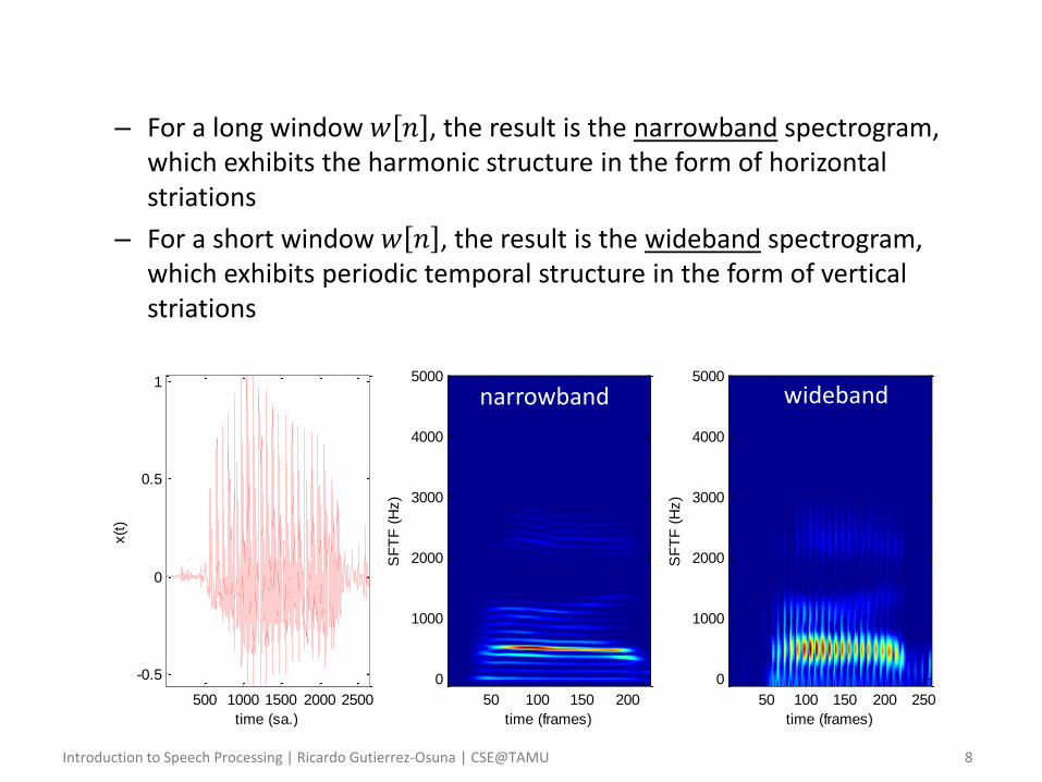
– For a long window 𝑤 𝑛 , the result is the narrowband spectrogram, which exhibits the harmonic structure in the form of horizontal striations

– For a short window 𝑤 𝑛 , the result is the wideband spectrogram, which exhibits periodic temporal structure in the form of vertical striations

500 1000 1500 2000 2500

-0.5

0

0.5

1

time (sa.)

x(t

)

time (frames)

SF

TF

(H

z)

50 100 150 200

5000

4000

3000

2000

1000

0

time (frames)

SF

TF

(H

z)

50 100 150 200 250

5000

4000

3000

2000

1000

0

narrowband wideband


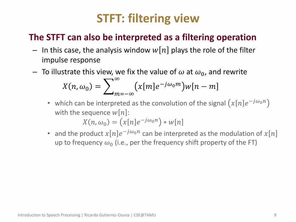
STFT: filtering view

• The STFT can also be interpreted as a filtering operation – In this case, the analysis window 𝑤 𝑛 plays the role of the filter

impulse response

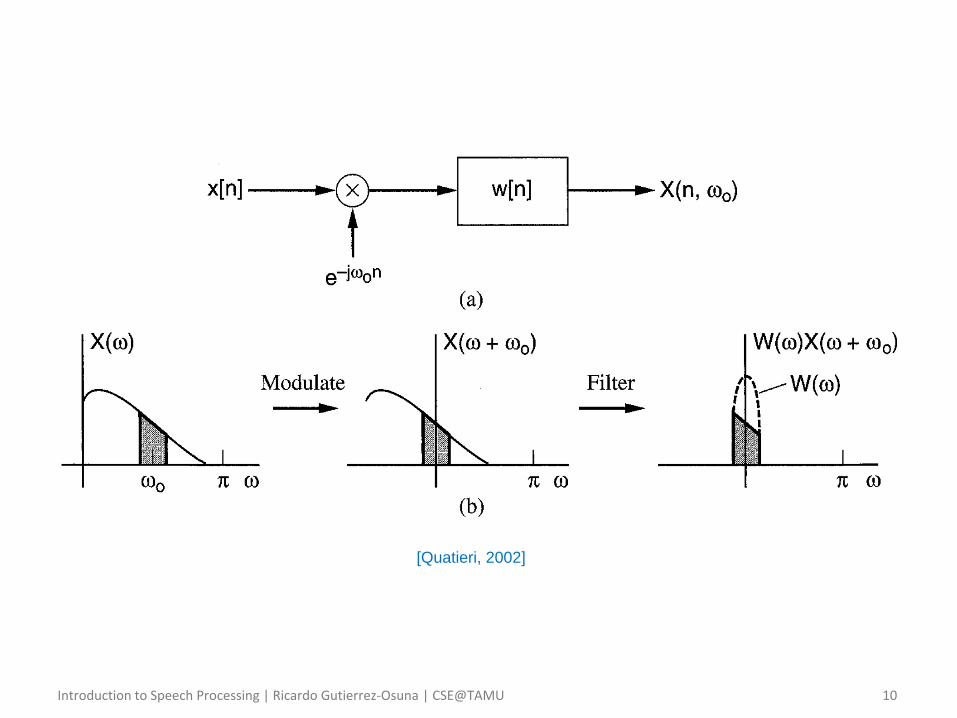
– To illustrate this view, we fix the value of 𝜔 at 𝜔0, and rewrite

𝑋 𝑛, 𝜔0 = 𝑥 𝑚 𝑒−𝑗𝜔0𝑚 𝑤 𝑛 − 𝑚∞

𝑚=−∞

• which can be interpreted as the convolution of the signal 𝑥 𝑛 𝑒−𝑗𝜔0𝑛

with the sequence 𝑤 𝑛 :

𝑋 𝑛, 𝜔0 = 𝑥 𝑛 𝑒−𝑗𝜔0𝑛 ∗ 𝑤 𝑛

• and the product 𝑥 𝑛 𝑒−𝑗𝜔0𝑛 can be interpreted as the modulation of 𝑥 𝑛 up to frequency 𝜔0 (i.e., per the frequency shift property of the FT)


[Quatieri, 2002]


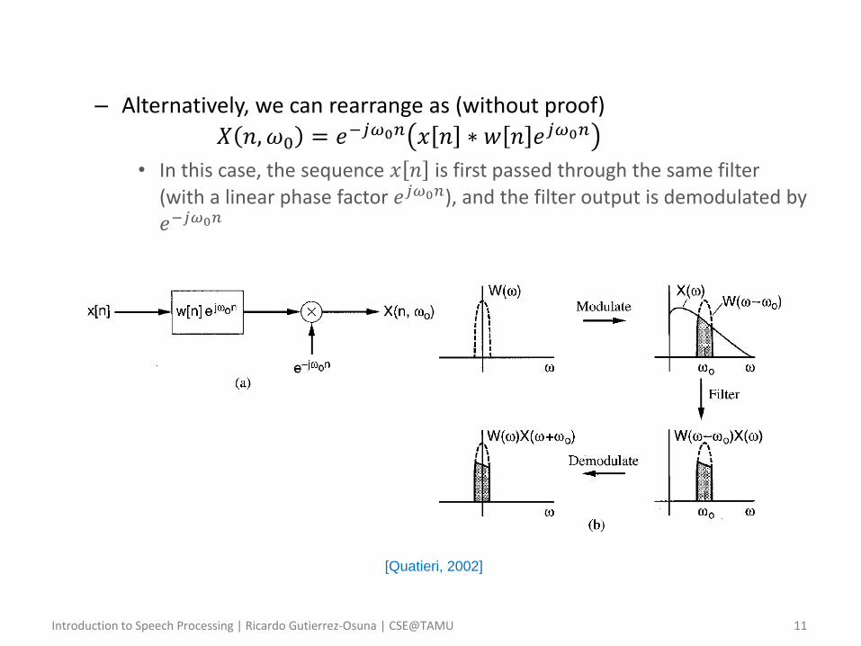
– Alternatively, we can rearrange as (without proof)

𝑋 𝑛, 𝜔0 = 𝑒−𝑗𝜔0𝑛 𝑥 𝑛 ∗ 𝑤 𝑛 𝑒𝑗𝜔0𝑛

• In this case, the sequence 𝑥 𝑛 is first passed through the same filter (with a linear phase factor 𝑒𝑗𝜔0𝑛), and the filter output is demodulated by 𝑒−𝑗𝜔0𝑛

[Quatieri, 2002]


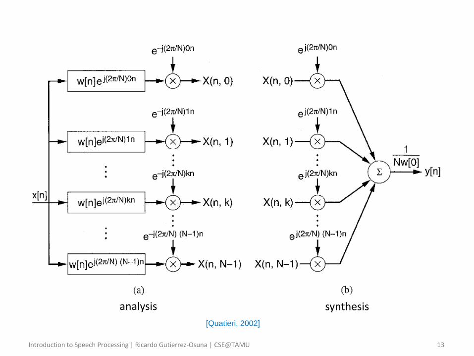
– This later rearrangement allows us to interpret the discrete STFT as the output of a filter bank

𝑋 𝑛, 𝑘 = 𝑒−𝑗2𝜋𝑁

𝑘𝑛 𝑥 𝑛 ∗ 𝑤 𝑛 𝑒−𝑗2𝜋𝑁

𝑘𝑛

• Note that each filter is acting as a bandpass filter centered around its selected frequency

– Thus, the discrete STFT can be viewed as a collection of sequences, each corresponding to the frequency components of 𝑥 𝑛 falling within a particular frequency band

• This filtering view is shown in the next slide, both from the analysis side and from the synthesis (reconstruction) side


[Quatieri, 2002]

analysis synthesis


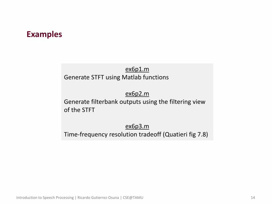
• Examples

ex6p1.m Generate STFT using Matlab functions

ex6p2.m Generate filterbank outputs using the filtering view of the STFT

ex6p3.m Time-frequency resolution tradeoff (Quatieri fig 7.8)


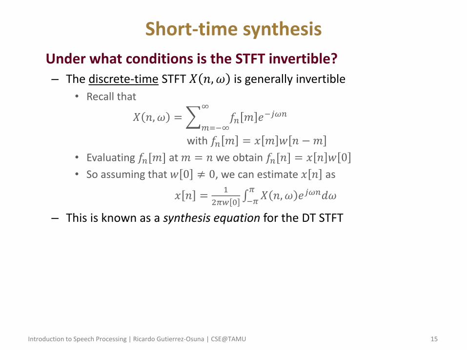
Short-time synthesis

• Under what conditions is the STFT invertible? – The discrete-time STFT 𝑋 𝑛, 𝜔 is generally invertible

• Recall that

𝑋 𝑛, 𝜔 = 𝑓𝑛 𝑚 𝑒−𝑗𝜔𝑛∞

𝑚=−∞

with 𝑓𝑛 𝑚 = 𝑥 𝑚 𝑤 𝑛 − 𝑚

• Evaluating 𝑓𝑛[𝑚] at 𝑚 = 𝑛 we obtain 𝑓𝑛[𝑛] = 𝑥 𝑛 𝑤 0

• So assuming that 𝑤 0 ≠ 0, we can estimate 𝑥 𝑛 as

𝑥 𝑛 =1

2𝜋𝑤 0 𝑋 𝑛, 𝜔 𝑒𝑗𝜔𝑛𝑑𝜔

𝜋

−𝜋

– This is known as a synthesis equation for the DT STFT


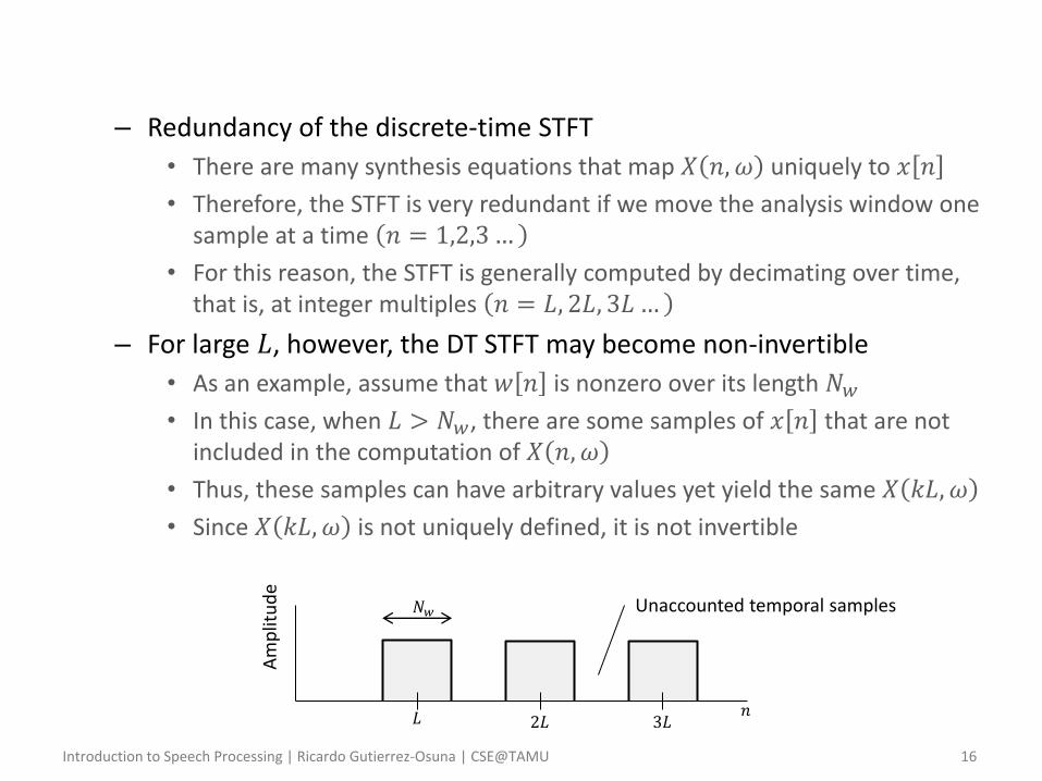
– Redundancy of the discrete-time STFT

• There are many synthesis equations that map 𝑋 𝑛, 𝜔 uniquely to 𝑥 𝑛

• Therefore, the STFT is very redundant if we move the analysis window one sample at a time 𝑛 = 1,2,3 …

• For this reason, the STFT is generally computed by decimating over time, that is, at integer multiples 𝑛 = 𝐿, 2𝐿, 3𝐿 …

– For large 𝐿, however, the DT STFT may become non-invertible

• As an example, assume that 𝑤 𝑛 is nonzero over its length 𝑁𝑤

• In this case, when 𝐿 > 𝑁𝑤, there are some samples of 𝑥 𝑛 that are not included in the computation of 𝑋 𝑛, 𝜔

• Thus, these samples can have arbitrary values yet yield the same 𝑋 𝑘𝐿, 𝜔

• Since 𝑋 𝑘𝐿, 𝜔 is not uniquely defined, it is not invertible

𝐿 2𝐿 3𝐿

𝑁𝑤 Unaccounted temporal samples

Am

plit

ud

e

𝑛


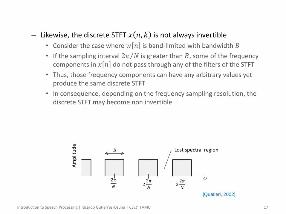
– Likewise, the discrete STFT 𝑥 𝑛, 𝑘 is not always invertible

• Consider the case where 𝑤 𝑛 is band-limited with bandwidth 𝐵

• If the sampling interval 2𝜋 𝑁 is greater than 𝐵, some of the frequency components in 𝑥 𝑛 do not pass through any of the filters of the STFT

• Thus, those frequency components can have any arbitrary values yet produce the same discrete STFT

• In consequence, depending on the frequency sampling resolution, the discrete STFT may become non invertible

2𝜋

𝑁 2

2𝜋

𝑁 3

2𝜋

𝑁

𝐵 Lost spectral region

Am

plit

ud

e

𝜔

[Quatieri, 2002]


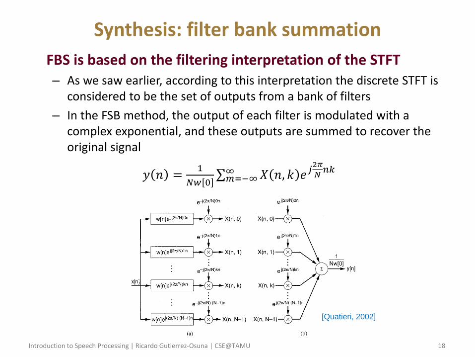
Synthesis: filter bank summation

• FBS is based on the filtering interpretation of the STFT – As we saw earlier, according to this interpretation the discrete STFT is

considered to be the set of outputs from a bank of filters

– In the FSB method, the output of each filter is modulated with a complex exponential, and these outputs are summed to recover the original signal

𝑦 𝑛 =1

𝑁𝑤 0 𝑋 𝑛, 𝑘 𝑒𝑗

2𝜋

𝑁𝑛𝑘∞

𝑚=−∞

[Quatieri, 2002]


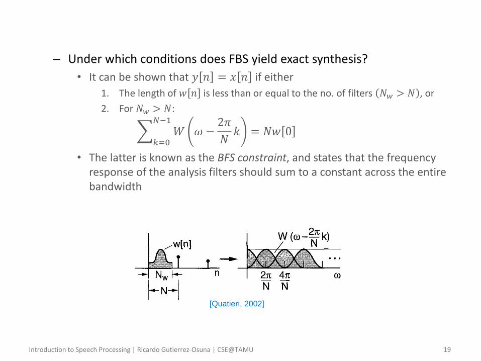
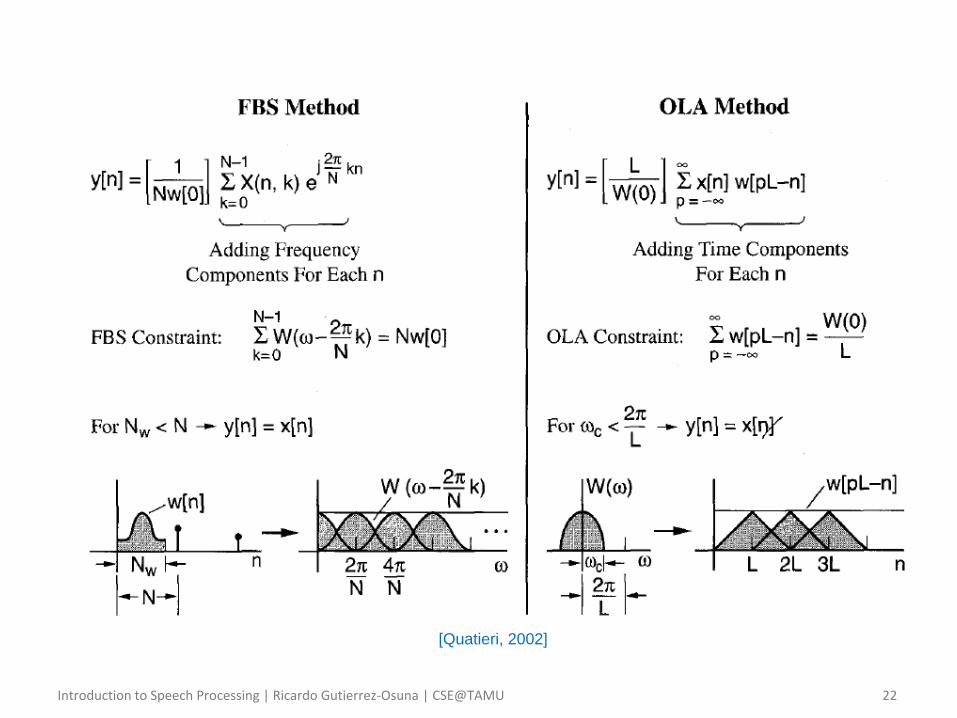
– Under which conditions does FBS yield exact synthesis?

• It can be shown that 𝑦 𝑛 = 𝑥 𝑛 if either

1. The length of 𝑤 𝑛 is less than or equal to the no. of filters 𝑁𝑤 > 𝑁 , or

2. For 𝑁𝑤 > 𝑁:

𝑊 𝜔 −2𝜋

𝑁𝑘 = 𝑁𝑤 0

𝑁−1

𝑘=0

• The latter is known as the BFS constraint, and states that the frequency response of the analysis filters should sum to a constant across the entire bandwidth

[Quatieri, 2002]


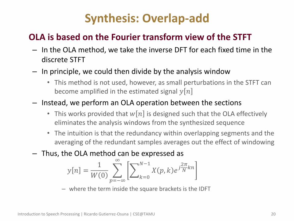
Synthesis: Overlap-add

• OLA is based on the Fourier transform view of the STFT – In the OLA method, we take the inverse DFT for each fixed time in the

discrete STFT

– In principle, we could then divide by the analysis window

• This method is not used, however, as small perturbations in the STFT can become amplified in the estimated signal 𝑦 𝑛

– Instead, we perform an OLA operation between the sections

• This works provided that 𝑤 𝑛 is designed such that the OLA effectively eliminates the analysis windows from the synthesized sequence

• The intuition is that the redundancy within overlapping segments and the averaging of the redundant samples averages out the effect of windowing

– Thus, the OLA method can be expressed as

𝑦 𝑛 =1

𝑊 0 𝑋 𝑝, 𝑘 𝑒𝑗

2𝜋𝑁

𝑘𝑛𝑁−1

𝑘=0

∞

𝑝=−∞

– where the term inside the square brackets is the IDFT


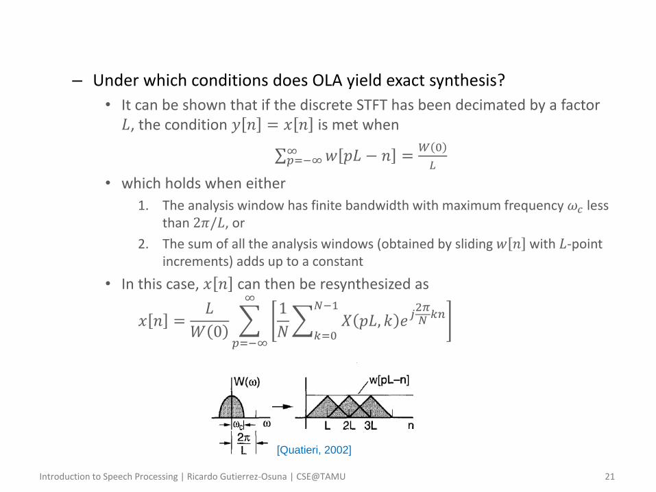
– Under which conditions does OLA yield exact synthesis?

• It can be shown that if the discrete STFT has been decimated by a factor 𝐿, the condition 𝑦 𝑛 = 𝑥 𝑛 is met when

𝑤 𝑝𝐿 − 𝑛∞𝑝=−∞ =

𝑊 0

𝐿

• which holds when either

1. The analysis window has finite bandwidth with maximum frequency 𝜔𝑐 less than 2𝜋/𝐿, or

2. The sum of all the analysis windows (obtained by sliding 𝑤 𝑛 with 𝐿-point increments) adds up to a constant

• In this case, 𝑥 𝑛 can then be resynthesized as

𝑥 𝑛 =𝐿

𝑊 0

1

𝑁 𝑋 𝑝𝐿, 𝑘 𝑒𝑗

2𝜋𝑁

𝑘𝑛𝑁−1

𝑘=0

∞

𝑝=−∞

[Quatieri, 2002]


[Quatieri, 2002]


STFT magnitude

• The spectrogram (STFT magnitude) is widely used in speech – For one, evidence suggests that the human ear extracts information

strictly from a spectrogram representation of the speech signal

– Likewise, trained researchers can visually “read” spectrograms, which further indicates that the spectrogram retains most of the information in the speech signal (at least at the phonetic level)

– Hence, one may question whether the original signal 𝑥 𝑛 can be recovered from 𝑋 𝑛, 𝜔 , that is, by ignoring phase information

• Inversion of the STFTM – Several methods may be used to estimate 𝑥 𝑛 from the STFTM

– Here we focus on a fairly intuitive least-squares approximation


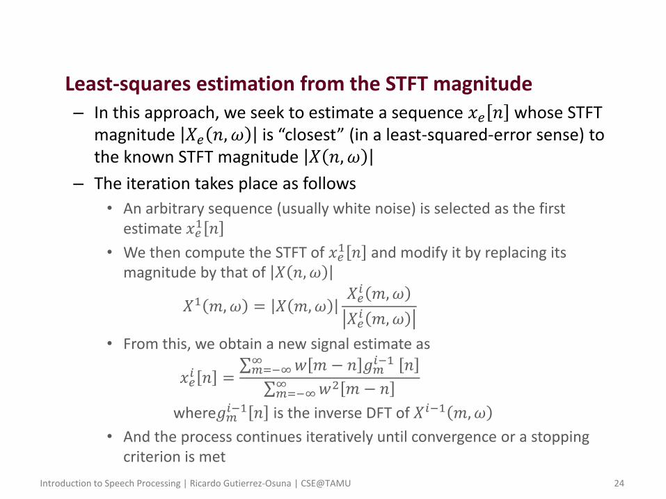
• Least-squares estimation from the STFT magnitude – In this approach, we seek to estimate a sequence 𝑥𝑒 𝑛 whose STFT

magnitude 𝑋𝑒 𝑛, 𝜔 is “closest” (in a least-squared-error sense) to the known STFT magnitude 𝑋 𝑛, 𝜔

– The iteration takes place as follows

• An arbitrary sequence (usually white noise) is selected as the first estimate 𝑥𝑒

1 𝑛

• We then compute the STFT of 𝑥𝑒1 𝑛 and modify it by replacing its

magnitude by that of 𝑋 𝑛, 𝜔

𝑋1 𝑚, 𝜔 = 𝑋 𝑚, 𝜔𝑋𝑒

𝑖 𝑚, 𝜔

𝑋𝑒𝑖 𝑚, 𝜔

• From this, we obtain a new signal estimate as

𝑥𝑒𝑖 𝑛 =

𝑤 𝑚 − 𝑛 𝑔𝑚𝑖−1 𝑛∞

𝑚=−∞

𝑤2 𝑚 − 𝑛∞𝑚=−∞

where𝑔𝑚𝑖−1 𝑛 is the inverse DFT of 𝑋𝑖−1 𝑚, 𝜔

• And the process continues iteratively until convergence or a stopping criterion is met


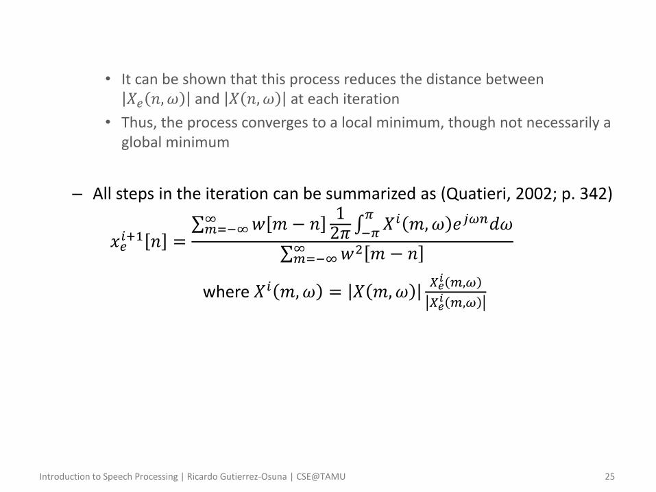
• It can be shown that this process reduces the distance between 𝑋𝑒 𝑛, 𝜔 and 𝑋 𝑛, 𝜔 at each iteration

• Thus, the process converges to a local minimum, though not necessarily a global minimum

– All steps in the iteration can be summarized as (Quatieri, 2002; p. 342)

𝑥𝑒𝑖+1 𝑛 =

𝑤 𝑚 − 𝑛12𝜋 𝑋𝑖 𝑚, 𝜔 𝑒𝑗𝜔𝑛𝑑𝜔

𝜋

−𝜋∞𝑚=−∞

𝑤2 𝑚 − 𝑛∞𝑚=−∞

where 𝑋𝑖 𝑚, 𝜔 = 𝑋 𝑚, 𝜔𝑋𝑒

𝑖 𝑚,𝜔

𝑋𝑒𝑖 𝑚,𝜔


• Example

ex6p4.m Estimate a signal from its STFT magnitude

Documents

L6: Short-time Fourier analysis and synthesisresearch.cs.tamu.edu/prism/lectures/sp/l6.pdf · L6: Short-time Fourier analysis and synthesis