Embed Size (px)
Citation preview
L4 Graphical Solution
• Homework• See new Revised Schedule• Review• Graphical Solution Process• Special conditions• Summary
1
Read 4.1-4.2 for W
4.3-4.4.2 for M
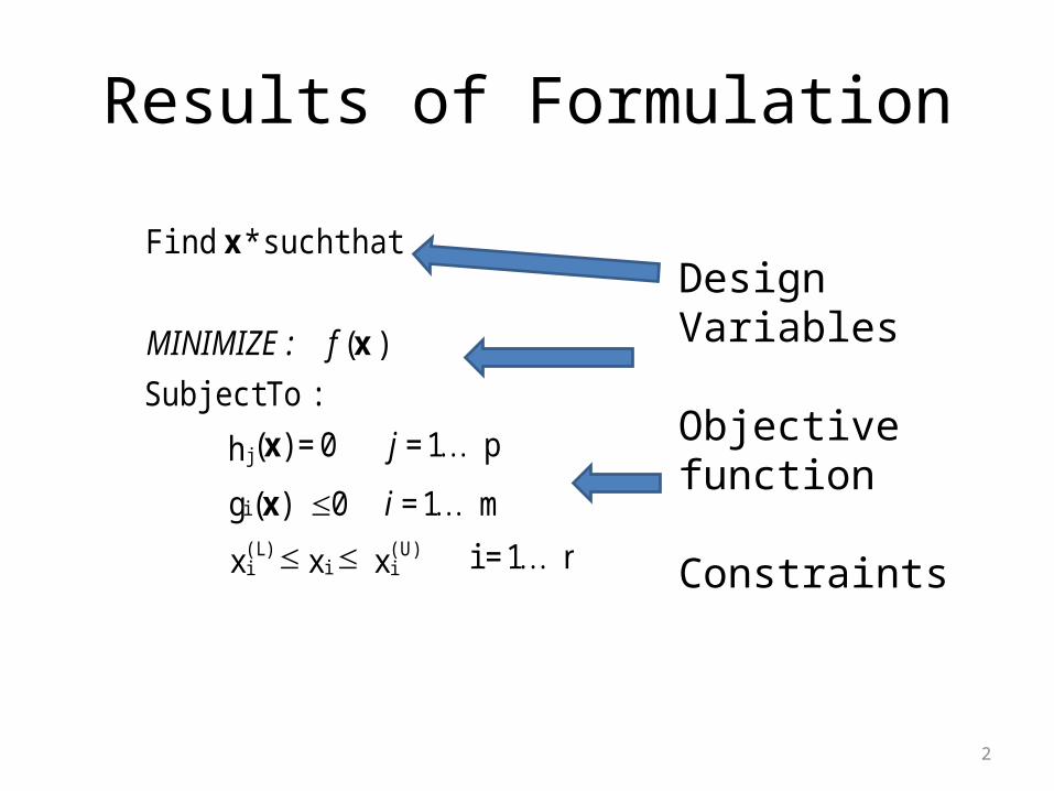
Results of Formulation
2
n1=i x x x
m1= 0 )(g
p1= 0 =)(h
) (
: ToSubject
thatsuch*Find
) (Uii
) (Li
i
j
i
j
f :MINIMIZE
x
x
x
xDesign Variables
Objective function
Constraints
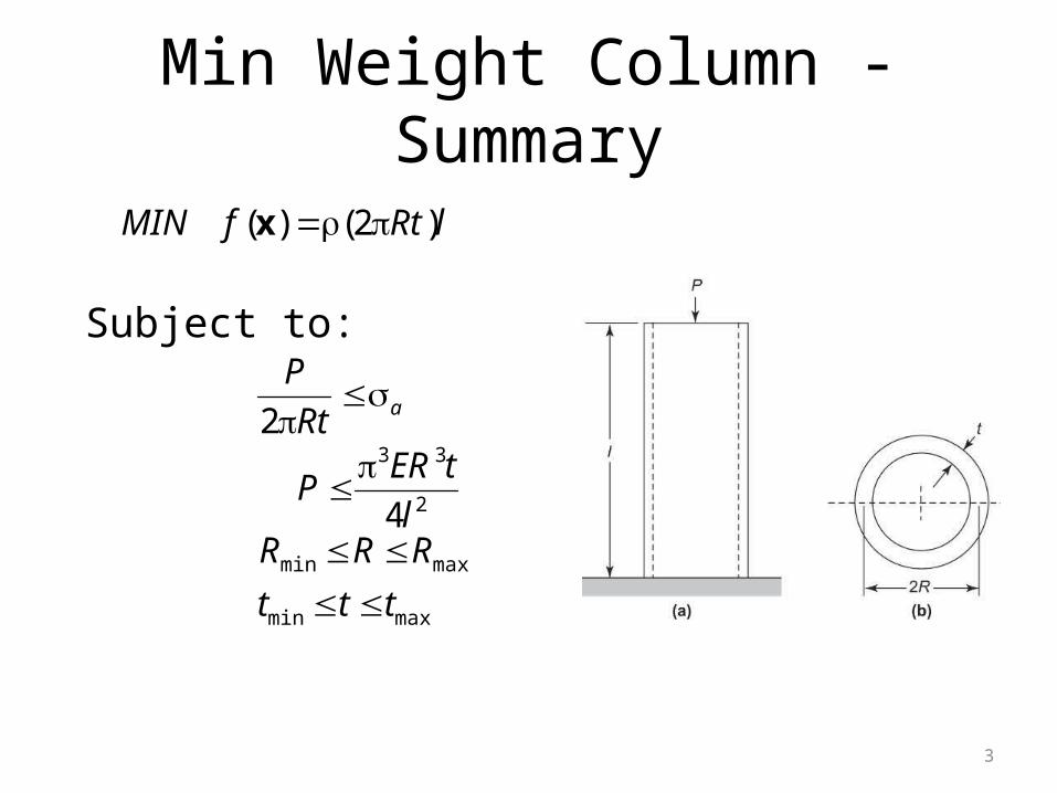
Min Weight Column - Summary
3
lRtfMIN )2()( x
Subject to:
aRt
P
2
2
33
4l
tERP
maxmin
maxmin
ttt
RRR
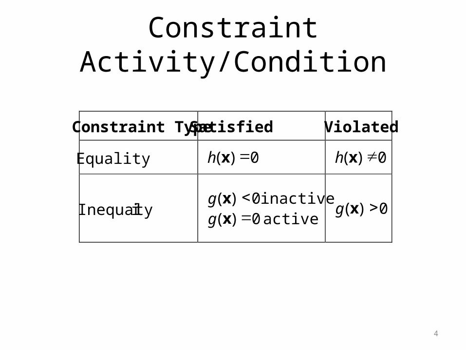
Constraint Activity/Condition
4
Constraint Type Satisfied Violated
Equality 0)( xh 0)( xh
Inequality inactive0)( xg active0)( xg
0)( xg
Graphical Solution
5
1. Sketch coordinate system2. Plot constraints3. Determine feasible region4. Plot f(x) contours 5. Find opt solution x* & opt value f(x*)
6
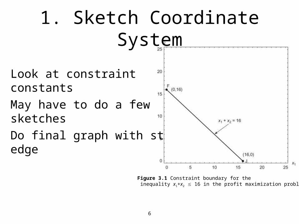
Figure 3.1 Constraint boundary for the inequality x1+x2 16 in the profit maximization problem.
Look at constraint constantsMay have to do a few sketchesDo final graph with st edge
1. Sketch Coordinate System
7
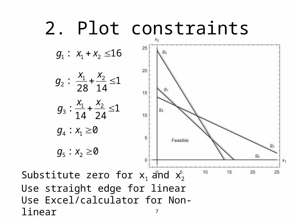
2. Plot constraints16: 211 xxg
11428
: 212
xxg
12414
: 213
xxg
0: 14 xg
0: 25 xg
Substitute zero for x1 and x2
Use straight edge for linear Use Excel/calculator for Non-linear
8
3. Determine feasible region
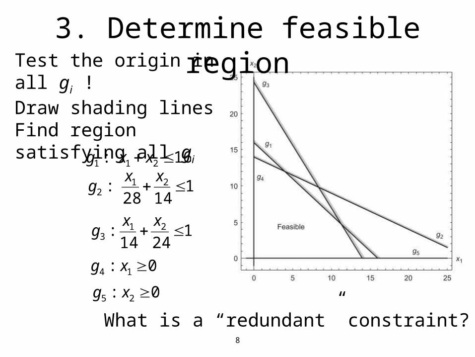
16: 211 xxg
11428
: 212
xxg
12414
: 213
xxg
0: 14 xg
0: 25 xg
Test the origin in all gi !Draw shading linesFind region satisfying all gi
What is a “redundant” constraint?
9
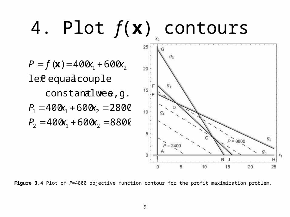
Figure 3.4 Plot of P=4800 objective function contour for the profit maximization problem.
4. Plot f(x) contours
8800600400
2800600400
e.g. alues,constant v
couple a equal let
600400)(
212
211
21
xxP
xxP
P
xxfP x
10
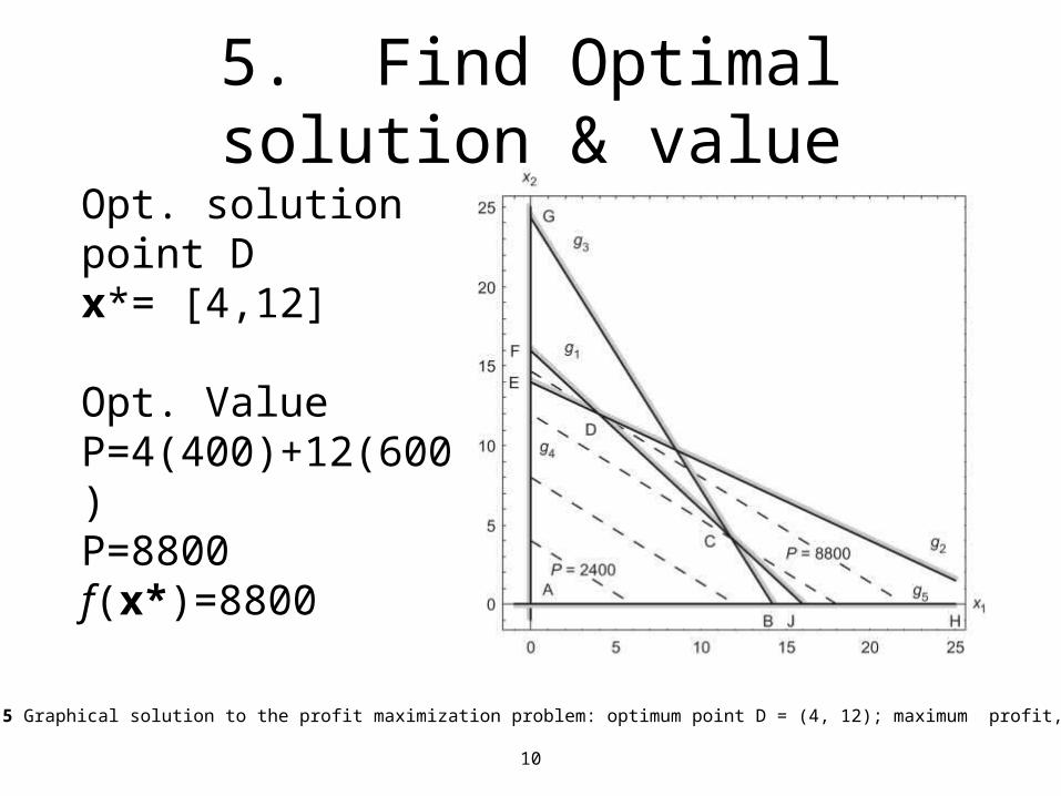
Figure 3.5 Graphical solution to the profit maximization problem: optimum point D = (4, 12); maximum profit, P = 8800.
5. Find Optimal solution & value
Opt. solutionpoint Dx*= [4,12]
Opt. ValueP=4(400)+12(600)P=8800f(x*)=8800
Graphical Solution
11
1. Sketch coordinate system2. Plot constraints3. Determine feasible region4. Plot f(x) contours (2 or 3)5. Find opt solution x* & opt value f(x*)
12
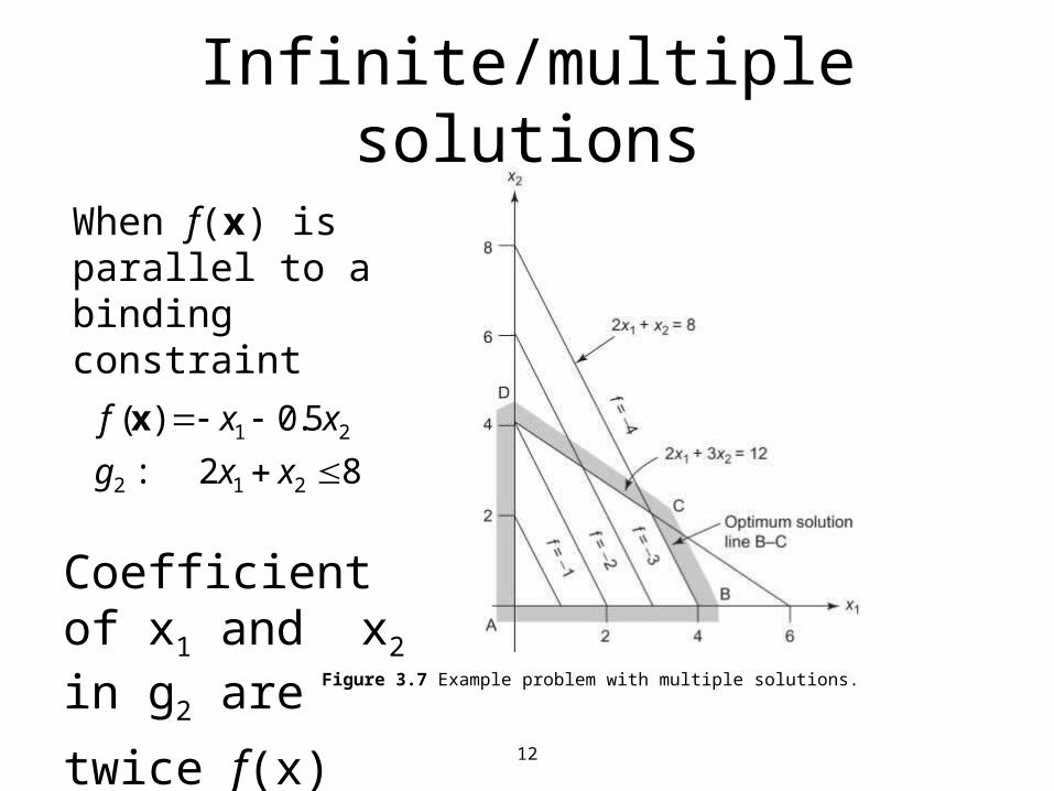
Figure 3.7 Example problem with multiple solutions.
Infinite/multiple solutions
82:
5.0)(
212
21
xxg
xxf x
When f(x) is parallel to a binding constraint
Coefficient of x1 and x2 in g2 are
twice f(x)
13
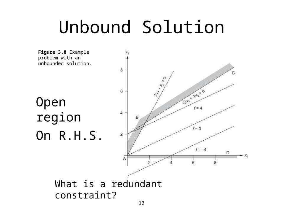
Figure 3.8 Example problem with an unbounded solution.
Unbound Solution
Open regionOn R.H.S.
What is a redundant constraint?
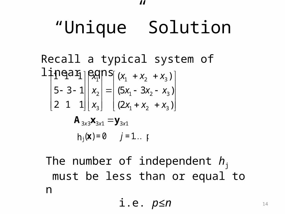
“Unique” Solution
14
p1= 0 =)(h j jx
Recall a typical system of linear eqns
131333
321
321
321
3
2
1
)2(
)35(
)(
112
135
111
xxx
xxx
xxx
xxx
x
x
x
yxA
The number of independent hj
must be less than or equal to n i.e. p≤n
15
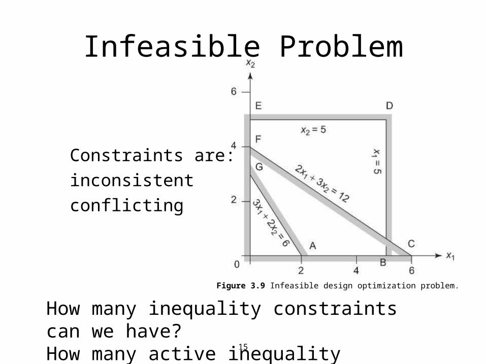
Figure 3.9 Infeasible design optimization problem.
Infeasible Problem
Constraints are:inconsistentconflicting
How many inequality constraints can we have?How many active inequality constraints?
16
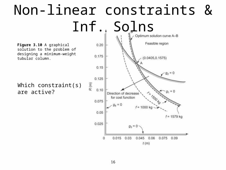
Figure 3.10 A graphical solution to the problem of designing a minimum-weight tubular column.
Non-linear constraints & Inf. Solns
Which constraint(s) are active?
Summary• Graphical solution – 5 step process• Feasible region may not exist resulting in
an infeasible problem• When obj function is ll to active/binding gi
an infinite number of solutions exist• Feasible region may be unbounded• An unbounded region may result in an
unbounded solution
17