Embed Size (px)
Citation preview
L2-Invariants forSelf-Similar CW-Complexes
Dissertation
for the award of the degree
“Doctor rerum naturalium” (Dr. rer. nat.)
of the Georg-August-Universitat Gottingen
within the doctoral program Mathematical Sciences
of the Georg-August University School of Science
(GAUSS)
submitted by
Engelbert Peter Suchla
from Braunschweig
Gottingen, 2020
Thesis committee
Prof. Dr. Thomas Schick,Mathematisches Institut, Georg-August-Universitat Gottingen
Prof. Dr. Dorothea Bahns,Mathematisches Institut, Georg-August-Universitat Gottingen
Members of the Examination Board
Reviewer: Prof. Dr. Thomas Schick,Mathematisches Institut, Georg-August-Universitat Gottingen
Second Reviewer: Prof. Dr. Dorothea Bahns,Mathematisches Institut, Georg-August-Universitat Gottingen
Further members of the Examination Board:
Prof. Dr. Laurent Bartholdi,Mathematisches Institut, Georg-August-Universitat Gottingen
Prof. Dr. Stephan Huckemann,Institut fur Mathematische Stochastik, Georg-August-Universitat Gottingen
Prof. Dr. Ralf Meyer,Mathematisches Institut, Georg-August-Universitat Gottingen
Prof. Dr. Gerlind Plonka-Hoch,Institut fur Numerische und Angewandte Mathematik,Georg-August-Universitat Gottingen
Date of the oral examination
7 October 2020
Acknowledgements
I would like to thank my advisor, Prof. Dr. Thomas Schick, for sending meon this mathematical journey. His enthusiastically shared knowledge and
neverending support made this thesis possible.
I would like to thank my second advisor, Prof. Dr. Dorothea Bahns, forfruitful discussions, insightful advice, and always having an open ear for me.
I would like to thank Prof. Dr. Gabor Elek und Dr. Lukasz Grabowski for theinvitation to Lancaster and for showing me their mathematical point of view.
I would like to thank my family, who are always there for me when I needthem most.
Finally, my thanks go to the German Research Foundation (DFG), whofinancially supported this thesis through the Research Training Group 1493“Mathematical structures in modern quantum physics” at the University of
Gottingen.

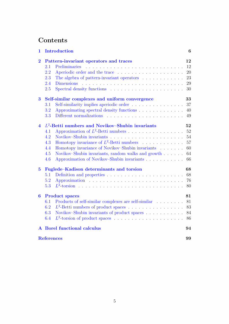
Contents
1 Introduction 6
2 Pattern-invariant operators and traces 122.1 Preliminaries . . . . . . . . . . . . . . . . . . . . . . . . . . . . 122.2 Aperiodic order and the trace . . . . . . . . . . . . . . . . . . . 202.3 The algebra of pattern-invariant operators . . . . . . . . . . . . 232.4 Dimensions . . . . . . . . . . . . . . . . . . . . . . . . . . . . . 292.5 Spectral density functions . . . . . . . . . . . . . . . . . . . . . 30
3 Self-similar complexes and uniform convergence 333.1 Self-similarity implies aperiodic order . . . . . . . . . . . . . . . 373.2 Approximating spectral density functions . . . . . . . . . . . . . 403.3 Different normalizations . . . . . . . . . . . . . . . . . . . . . . 49
4 L2-Betti numbers and Novikov–Shubin invariants 524.1 Approximation of L2-Betti numbers . . . . . . . . . . . . . . . . 524.2 Novikov–Shubin invariants . . . . . . . . . . . . . . . . . . . . . 544.3 Homotopy invariance of L2-Betti numbers . . . . . . . . . . . . 574.4 Homotopy invariance of Novikov–Shubin invariants . . . . . . . 604.5 Novikov–Shubin invariants, random walks and growth . . . . . . 644.6 Approximation of Novikov–Shubin invariants . . . . . . . . . . . 66
5 Fuglede–Kadison determinants and torsion 685.1 Definition and properties . . . . . . . . . . . . . . . . . . . . . . 685.2 Approximation . . . . . . . . . . . . . . . . . . . . . . . . . . . 765.3 L2-torsion . . . . . . . . . . . . . . . . . . . . . . . . . . . . . . 80
6 Product spaces 816.1 Products of self-similar complexes are self-similar . . . . . . . . 816.2 L2-Betti numbers of product spaces . . . . . . . . . . . . . . . . 836.3 Novikov–Shubin invariants of product spaces . . . . . . . . . . . 846.4 L2-torsion of product spaces . . . . . . . . . . . . . . . . . . . . 86
A Borel functional calculus 94
References 99
5
1 Introduction
Algebraic topology means to use algebraic tools to answer topological ques-tions. We take some description of a topological space, often in combinatorialor geometrical terms, and turn it into an algebraic structure. That structuretends to be large and unsightly at first, but the algebraic machinery will even-tually distill it down to succinct statements about the topology of our space.And hopefully, the result will be independent of the choice of the descriptionwe gave in the beginning or the algebraic detours we took in between.
Homology theory is one of the two most important such machines.1 Mosttopological spaces can be considered as cell complexes: they can be built upfrom vertices (0-cells), edges (1-cells), faces (2-cells), etc. Let EjX be the setof j-cells of a space X, and C[EjX] be the abstract vector space they generate.Then, the geometric description of X translates into a series of boundary maps
. . .→ C[E3X]∂3−−→ C[E2X]
∂2−−→ C[E1X]∂1−−→ C[E0X]
where ∂j sends each j-cell to the sum (or, depending on the orientations, thedifference) of the (j − 1)-cells that make up its boundary.
Let us combine the boundary maps into Laplacian operators :
∆j = ∂∗j ∂j + ∂j+1∂∗j+1 : C[EjX]→ C[EjX].
The kernels of these operators are the homology groups of X:
Hj(X;C) = ker ∆j.
These are not only much smaller than the vector spaces C[EjX], but also inde-pendent of the precise geometric description of the space – they only measuretopological properties. Their dimensions are the Betti numbers of X:
βj(X) = dimCHj(X;C) = dimC(ker ∆j).
L2-invariants are an approach to homology for spaces with infinitely manycells. Completing the vector spaces C[EjX] yields Hilbert spaces `2(EjX),and the Laplacians extend (under certain conditions) to bounded operatorson these spaces. Unlike in the finite case, these new Laplacians usually havea continuous spectrum, and it turns out that the entire spectrum – not justthe size of the kernel – can carry topological information. To measure this, werequire a spectral density function2, which, for any λ ≥ 0, quantifies the sizeof the largest subspace on which the operator’s norm is bounded by λ.
Defining such a function poses one main challenge: to describe the size ofinfinite-dimensional spaces with finite numbers.
1The other being homotopy theory.2Often also called the integrated density of states.
6
Periodic spaces
Let us call a complex X periodic if there are a finite subcomplex K and agroup G acting freely and cellularly on X such that G · K = X. Then theinfinitely many cells of X form finitely many G-orbits, and each `2(EjX) canbe identified with a space (`2G)n for some n ∈ N.
For any G-equivariant operator T ∈ B(`2(EjX)), the value of 〈σ, Tσ〉 (forσ ∈ EjX) is constant along any G-orbit! Taking the trace over only onerepresentative per orbit yields the von Neumann trace
trN (G)(T ) =∑
[σ]∈(EjX)/G
〈σ, Tσ〉 .
The Laplacian is G-equivariant, since it only depends on the geometric struc-ture of the space that is preserved by the G-action. Furthermore, the G-equivariant operators form a von Neumann algebra (that is, a weakly closedC∗-algebra), so any spectral projections χ[0,λ](∆j) are G-equivariant as well,and we can define the desired spectral density function as
F (∆j)(λ) = trN (G)
(χ[0,λ](∆j)
).
Especially, its value at zero measures the size of the kernel of ∆j, and consti-tutes the j-th L2-Betti number of X:
b(2)j (X) = F (∆j)(0) = trN (G)(projker ∆j
).
This is the starting point of the theory of L2-invariants, invented by Atiyah[Ati76].
Novikov and Shubin [NS86] found a topological invariant that quantifiesthe “almost-kernel” (the part of the spectrum very close to zero):
αj(X) = limλ→0
log(F (∆j)(λ)− F (∆j)(0))
log(λ).
Finally, the spectral density function allows to define a determinant in thesense of Fuglede and Kadison [FK52] for such operators.
L2-invariants have been studied in great detail (see [Luc02] for an extensivetreatment, and [Kam19] for an overview). However, their construction reliedheavily on the existence of a suitable group action on the space – in otherwords, on periodicity.
However, there is a completely different approach to these invariants, inwhich the group structure fades into the background: approximation.
Let us again write X = G · K with a compact subcomplex K. At first,the L2-Betti numbers of X have little to nothing in common with the Bettinumbers of K or the quotient space X/G: Evaluating the Laplacian on a cellnear the boundary of K will produce drastically different results dependingon whether crossing that boundary will lead into another copy of K (whenwe are working on X), or back into K itself (when we are working on X/G),
7
or into nothingness (when we are working just on K). Thus, if we want to“approximate” X by a finite subcomplex K, the boundary of K will be wherethe similarities end. Consequently, K will only show similar properties to Xif its boundary is insignificant compared to its interior!
This is one of the many definitions of amenability : A space X is amenableif there is a Følner sequence of finite subspaces
K0 ⊆ K1 ⊆ K2 ⊆ K3 ⊆ . . . ⊆ X,⋃m
Km = X,
such that, in some suitable measure, the share of points in Km that are closeto its boundary converges to zero.
In such an amenable periodic space, Dodziuk and Mathai [DM98] provedthat the L2-Betti numbers can indeed be obtained from ordinary Betti numbersof larger and larger subspaces: If nm counts how many representatives of eachG-orbit lie in Km, then
b(2)j (X;G) = lim
m→∞
βj(Km)
nm, (∗)
and their proof can be extended to approximate not just L2-Betti numbers,but whole spectral density functions.
In this final formula, the group structure barely appears any more (only inthe normalization factor nm, which could be replaced by e. g. the number ofcells in Km). Thus, we can begin to ask the question: Can this limit exist ifthere is no group action on X?
Aperiodic spaces
The existence of the limit (∗) depends mainly on two factors. On the onehand, it needs amenability: For example, any d-regular tree with d ≥ 3 hasa positive first L2-Betti number, while each finite subtree of it has β1 = 0.On the other hand, it requires that finite subcomplexes are in some sense“representative” for the whole space: any structure that can be found in thespace must be found at a similar frequency in every sufficiently large finitesubspace. Periodic spaces certainly satisfy this condition – but they are notthe only ones.
A first such observation was made by Geerse and Hof [GH91], who studiedself-similar tilings of Rn (such as the decidedly non-periodic Penrose tilings)in an effort to model the physical properties of quasicrystals, and proved theexistence of various thermodynamic means.
Kellendonk [Kel95] studied the same tilings from a mathematical pointof view. He used the geometry of the tiling itself to define a C∗-algebra ofoperators, and established the existence of a spectral density function for suchoperators.
Cipriani, Guido and Isola [CGI09] constructed self-similar complexes :Beginning with a finite CW-complex K0, define a sequence of complexes
Km, where each Km is the union of several copies of Km−1, glued together
8
along a small number of overlapping cells. Identifying each Km with one partof Km+1, one then obtains the self-similar space as the union
X =∞⋃m=0
Km.
Under the condition that (Km) is a Følner sequence in X, Cipriani, Guidoand Isola were able to define traces for “geometric” operators on such spaces.However, geometric operators do not form a von Neumann algebra, and theirspectral projections are not geometric. Thus, with no access to spectral densityfunctions, Cipriani, Guido and Isola defined Betti numbers as
β(∆) = limt→∞
tr(e−t∆)
and Novikov–Shubin invariants as
α(∆) = 2 limt→∞
log(tr(e−t∆)− β(∆))
− log(t).
They proved that the Euler characteristics of Km converged to that of X, andcalculated Novikov–Shubin invariants for certain complexes.
Meanwhile, Elek [Ele06] gave a precise definition for aperiodic order ongeneral graphs (that is, one-dimensional complexes): In a graph, let the r-pattern of a vertex v be the isomorphism class of the (rooted) graph spannedby all the vertices that are at most r steps away from v. Then a graph hasaperiodic order if every such pattern appears at a well-defined frequency: inany Følner sequence, the share of vertices with this pattern converges to thesame number.
Elek then defined the algebra of pattern-invariant operators on the space`2(vertices), whose values on a vertex only depend on the pattern of the vertex,and proved that their spectral density functions can be obtained as a uniformlimit over finite subgraphs – provided that the graph has aperiodic order. (Thepattern-invariant operators do not form a von Neumann algebra either; Elekavoided this problem by passing to the Gelfand–Naimark–Segal construction– an abstract algebra based on the representation of an algebra on “itself”.)
In a second paper [Ele08], Elek found a large class of graphs that actuallysatisfy this condition by relating it to Benjamini–Schramm convergence of thegraphs themselves.
Content and results of this thesis
In this thesis, we combine and expand the ideas of Elek and Cipriani–Guido–Isola to define and study L2-invariants for self-similar complexes.
In Chapter 2, we extend Elek’s framework of aperiodic order to higher-dimensional complexes. This includes the existence of a trace for geometricoperators on such complexes, and the extension of the trace to a suitable von
9
Neumann algebra, which allows us to define spectral density functions for anysuch operators.
In Chapter 3, we show that Cipriana–Guido–Isola’s self-similar complexesalways have aperiodic order, and prove the approximation theorem for spectraldensity functions:
Theorem (3.5 and 3.11). Let X be a self-similar complex with Følner sequence(Km), and let T ∈ B(`2(EjX)) be any geometric operator. Then the renor-malized spectral density functions of T |Km converge uniformly to the spectraldensity function of T .
In Chapter 4, we define L2-Betti numbers and Novikov–Shubin invariantsfor self-similar complexes, and we study their properties. Especially, we showthat the L2-Betti numbers of a self-similar complex are approximated by thoseof its subcomplexes and discuss this possibility for Novikov–Shubin invariants,and we prove that both of these are indeed invariant under self-similar homo-topies:
Theorem (4.13 and 4.14). Let X and Y be self-similar complexes that areself-similarly homotopy equivalent. Then we have
b(2)j (X) = c · b(2)
j (Y ) and αj(X) = αj(Y ) for all j,
where the constant
c = limm→∞
|EjLm||EjKm|
adjusts for the number of cells used in the specific cell structure of each complex.It is independent of the choice of self-similar Følner sequences (Km) for X and(Lm) for Y, as long as they fulfill Km ' Lm for all m ∈ N.
In Chapter 5, we discuss Fuglede–Kadison determinants of geometric op-erators. We can prove that these determinants in general share many of theproperties of their classical equivalents, especially multiplicativity, and thatthe Laplacians of self-similar complexes are of determinant class; this lets usalso define L2-torsion for self-similar complexes. Whether the determinants orthe torsion can be approximated in general remains an open question, but wecan show convergence for the Laplacians of some self-similar CW-complexes.
In Chapter 6, we show that the cartesian product of self-similar com-plexes is again such a complex, and we prove product formulas for all threeL2-invariants:
Theorem (6.3, 6.5 and 6.6). Let X and Y be self-similar complexes, andnormalize every trace by the numbers of vertices. Then we have:
(a) L2-Betti numbers fulfill the Kunneth formula:
b(2)` (X × Y ) =
∑j+k=`
b(2)j (X) · b(2)
k (Y ).
10
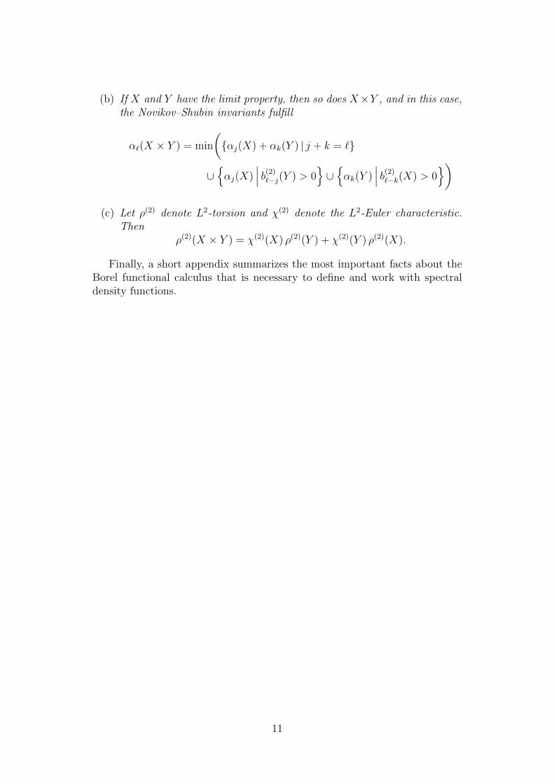
(b) If X and Y have the limit property, then so does X×Y , and in this case,the Novikov–Shubin invariants fulfill
α`(X × Y ) = min
(αj(X) + αk(Y ) | j + k = `
∪αj(X)
∣∣∣ b(2)`−j(Y ) > 0
∪αk(Y )
∣∣∣ b(2)`−k(X) > 0
)
(c) Let ρ(2) denote L2-torsion and χ(2) denote the L2-Euler characteristic.Then
ρ(2)(X × Y ) = χ(2)(X) ρ(2)(Y ) + χ(2)(Y ) ρ(2)(X).
Finally, a short appendix summarizes the most important facts about theBorel functional calculus that is necessary to define and work with spectraldensity functions.
11
2 Pattern-invariant operators and traces
Throughout this thesis, we aim to use geometrical (or topological) propertiesof spaces to ensure the analytical convergence of algebraic properties. In thischapter, we will lay the groundwork for all of that.
First, we will look at the geometric structure of regular CW-complexes andhow it translates into algebra. Then, we will define the concept of geometricoperators , that is, operators on the L2-chain groups whose values only dependon the geometric patterns of the space.
The most important geometric operators are the Laplacians of the space,and every L2-invariant will later be derived from their spectra. We thereforeturn to functional analysis to construct a tool that measures these spectra,namely, the spectral density function (or integrated density of states). Thisfunction is usually defined as the trace of the spectral projections of the op-erators – which poses two challenges: There is a priori no trace on the setof operators on an infinite-dimensional space, and spectral projections of geo-metric operators are in general not geometric.
Constructing a trace for the geometric operators themselves requires to takea mean over the infinite set of cells. To ensure such a mean is well-defined, wewill make use of the concept of aperiodic order : We will consider only spaceswhere every pattern appears with a well-defined frequency. (We will show inthe next chapter that self-similar complexes do indeed have this property.)In that situation, the defining property of geometric operators ensures theexistence of the trace.
The trace is unfortunately not weakly continuous, and it therefore does notsimply extend to the weak closure of the algebra of geometric operators (whichwould contain the spectral projections we are interested in). Instead, we willconstruct a different von Neumann algebra containing all geometric operatorsto which the trace can be extended. This will finally allow us to define thedesired spectral density functions.
2.1 Preliminaries
As a compromise between the algebraically simple, but rigid structure of sim-plicial complexes and the flexible, but algebraically complicated structure ofCW-complexes, we will be using regular CW-complexes . Let us briefly look attheir definition and most important properties.
Unless otherwise noted, every map of topological spaces will be assumedto be continuous.
2.1 Definition. Let X be a CW-complex, and denote by EjX the set of j-cellsof X. As a special case, if X is one-dimensional, it is a graph with vertex setE0X and edge set E1X.
X is the disjoint union of its cells. Denote by X(j) the j-skeleton of X,that is, the union of all cells of dimension ≤ j.
12
For any cell σ ∈ EjX, let fσ : Sj−1 → X(j−1) be the attaching map. It
extends to a map Fσ : Dj → X such that Fσ(Dj) = σ. Denote by ∂σ =fσ(Sj−1) the topological boundary of σ in X.
A subcomplex K ⊆ X is called full if, whenever K contains the boundaryof a cell σ of X, it also contains σ.
The complex X is regular if for each cell σ, the extended attaching mapFσ : Dj → σ ⊆ X is a homeomorphism onto its image.
The complex X is bounded if there is a constant C > 0 such that each cellσ ∈ EjX (for arbitrary j) fulfills
|ρ ∈ Ej−1X | ρ ⊆ ∂σ| ≤ C
and|τ ∈ Ej+1X |σ ⊆ ∂τ| ≤ C.
Regularity is a rather strong restriction for CW-complexes. On the onehand, it can necessitate much more complicated cell structures: For example,the n-sphere has a CW-structure with only two cells (a 0- and an n-cell) but itssmallest regular CW-structure consists of 2n + 1 cells (two of each dimensionbetween 0 and n).
On the other hand, regularity allows to treat the cells in a much moreintuitive way: For example, it allows us to say that the boundary of a cell σconsists of certain other cells, and it ensures that the closure of every cell is asubcomplex:
2.2 Lemma. Let X be a regular CW-complex. Let ρ ∈ Ej−1X and σ ∈ EjX.Then either ρ ⊆ ∂σ or ρ ∩ ∂σ = ∅.
Proof. Assume the contrary and choose a point
x ∈ ρ ∩ ∂σ ∩ ρ \ ∂σ.
(The intersection is nonempty because ρ is connected.) Since ∂σ is closed inX, we have x ∈ ∂σ.
Using the attaching map fσ : Sj−1 → ∂σ ⊆ X, define Ur = fσ(Br(f−1σ (x))),
where Br(ξ) means the open r-ball around ξ in Sj−1 ⊆ Rj. Each of the Ur isby definition homeomorphic to Dj−1 and contained in ∂σ.
If there were an r > 0 such that Ur ⊆ ρ, then this Ur would also be anopen neighborhood of x in ρ (since ρ itself is homeomorphic to a disc Dj−1).But then x could not be contained in ρ \ ∂σ – contradiction.
Thus, there is a sequence of points yr ∈ Ur that are not contained in ρ.Since it is compact, ∂σ intersects only finitely many cells, so we can assumethat all yr are contained in the same k-cell ρ′ (for some k ≤ j−1), and thereforex ∈ ρ′. However, by construction of the CW-complex, the open cell ρ must bedisjoint from the closure of any other cell of dimension ≤ j− 1, so this, too, isa contradiction.
2.3 Corollary. If S ⊆ X is a union of cells of X, then its closure S is asubcomplex of X.
13
Note that both this lemma and its corollary are false for general CW-complexes: For example, given a one-dimensional CW-complex X, one couldattach a 2-cell by mapping its entire boundary to a single point of X that isnot a 0-cell. Then the boundary of this cell contains one point of a 1-cell, butnot the rest of that cell, and its closure in X is not a subcomplex.
2.4 Remark. In fact, regular CW-complexes are relatively close to simplicialcomplexes. Allen Hatcher describes their relations as follows ([Hat02], p. 534):
“A CW complex is called regular if its characteristic maps can be chosento be embeddings. The closures of the cells are then homeomorphic to closedballs, and so it makes sense to speak of closed cells in a regular CW complex.The closed cells can be regarded as cones on their boundary spheres, and thesecone structures can be used to subdivide a regular CW complex into a regular∆-complex, by induction over skeleta. [...] The barycentric subdivision of aregular unordered ∆-complex is a simplicial complex.”
Therefore, working in a category of regular CW-complexes is very closeto working in the simplicial category. Compared to simplicial complexes, themain advantage of regular CW-complexes is their compatibility with productspaces, as the product of two regular cells is again a regular cell, while theproduct of two simplices is almost never a simplex.
For regular CW-complexes, the cellular chain complex takes a particularlysimple form: Write the chain groups as C[EjX] and the differential as
∂j : C[EjX]→ C[Ej−1X], σ 7→∑
ρ∈Ej−1X
[σ : ρ] ρ
with incidence numbers [σ : ρ] ∈ Z. Then we have:
2.5 Lemma. Let X be a regular CW-complex, σ ∈ EjX and ρ ∈ Ej−1X. Then
[σ : ρ] =
±1, if ρ ⊆ ∂σ,
0, otherwise
Proof. See [Suc16], Lemma 1.5.
As our goal is to consider L2-invariants, we will soon pass to the Hilbertspace completion of the chain groups, namely, `2(EjX). The properties ofboundedness and regularity together will ensure that the differentials extendto bounded operators on these spaces.
2.6 Definition. Let X be a regular CW-complex.Define the combinatorial distance of two j-cells σ, σ′ ∈ EjX as follows:
dcomb(σ, σ′) = 0 if and only if σ = σ′.
dcomb(σ, σ′) = 1 if σ 6= σ′ and there is a (j−1)-cell ρ such that ρ ⊆ ∂σ∩∂σ′or if there is a (j + 1)-cell τ such that σ ∪ σ′ ⊆ ∂τ .
14
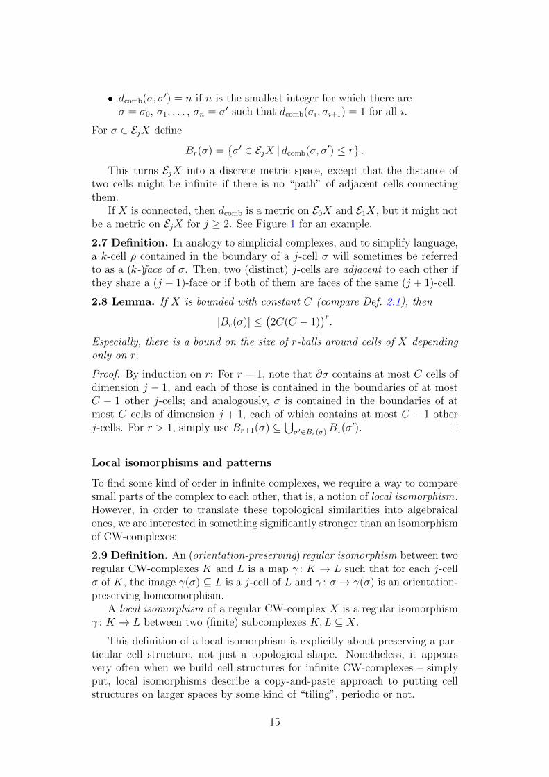
dcomb(σ, σ′) = n if n is the smallest integer for which there areσ = σ0, σ1, . . . , σn = σ′ such that dcomb(σi, σi+1) = 1 for all i.
For σ ∈ EjX define
Br(σ) = σ′ ∈ EjX | dcomb(σ, σ′) ≤ r .
This turns EjX into a discrete metric space, except that the distance oftwo cells might be infinite if there is no “path” of adjacent cells connectingthem.
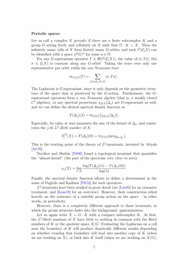
If X is connected, then dcomb is a metric on E0X and E1X, but it might notbe a metric on EjX for j ≥ 2. See Figure 1 for an example.
2.7 Definition. In analogy to simplicial complexes, and to simplify language,a k-cell ρ contained in the boundary of a j-cell σ will sometimes be referredto as a (k-)face of σ. Then, two (distinct) j-cells are adjacent to each other ifthey share a (j − 1)-face or if both of them are faces of the same (j + 1)-cell.
2.8 Lemma. If X is bounded with constant C (compare Def. 2.1), then
|Br(σ)| ≤(2C(C − 1)
)r.
Especially, there is a bound on the size of r-balls around cells of X dependingonly on r.
Proof. By induction on r: For r = 1, note that ∂σ contains at most C cells ofdimension j − 1, and each of those is contained in the boundaries of at mostC − 1 other j-cells; and analogously, σ is contained in the boundaries of atmost C cells of dimension j + 1, each of which contains at most C − 1 otherj-cells. For r > 1, simply use Br+1(σ) ⊆
⋃σ′∈Br(σ) B1(σ′).
Local isomorphisms and patterns
To find some kind of order in infinite complexes, we require a way to comparesmall parts of the complex to each other, that is, a notion of local isomorphism.However, in order to translate these topological similarities into algebraicalones, we are interested in something significantly stronger than an isomorphismof CW-complexes:
2.9 Definition. An (orientation-preserving) regular isomorphism between tworegular CW-complexes K and L is a map γ : K → L such that for each j-cellσ of K, the image γ(σ) ⊆ L is a j-cell of L and γ : σ → γ(σ) is an orientation-preserving homeomorphism.
A local isomorphism of a regular CW-complex X is a regular isomorphismγ : K → L between two (finite) subcomplexes K,L ⊆ X.
This definition of a local isomorphism is explicitly about preserving a par-ticular cell structure, not just a topological shape. Nonetheless, it appearsvery often when we build cell structures for infinite CW-complexes – simplyput, local isomorphisms describe a copy-and-paste approach to putting cellstructures on larger spaces by some kind of “tiling”, periodic or not.
15
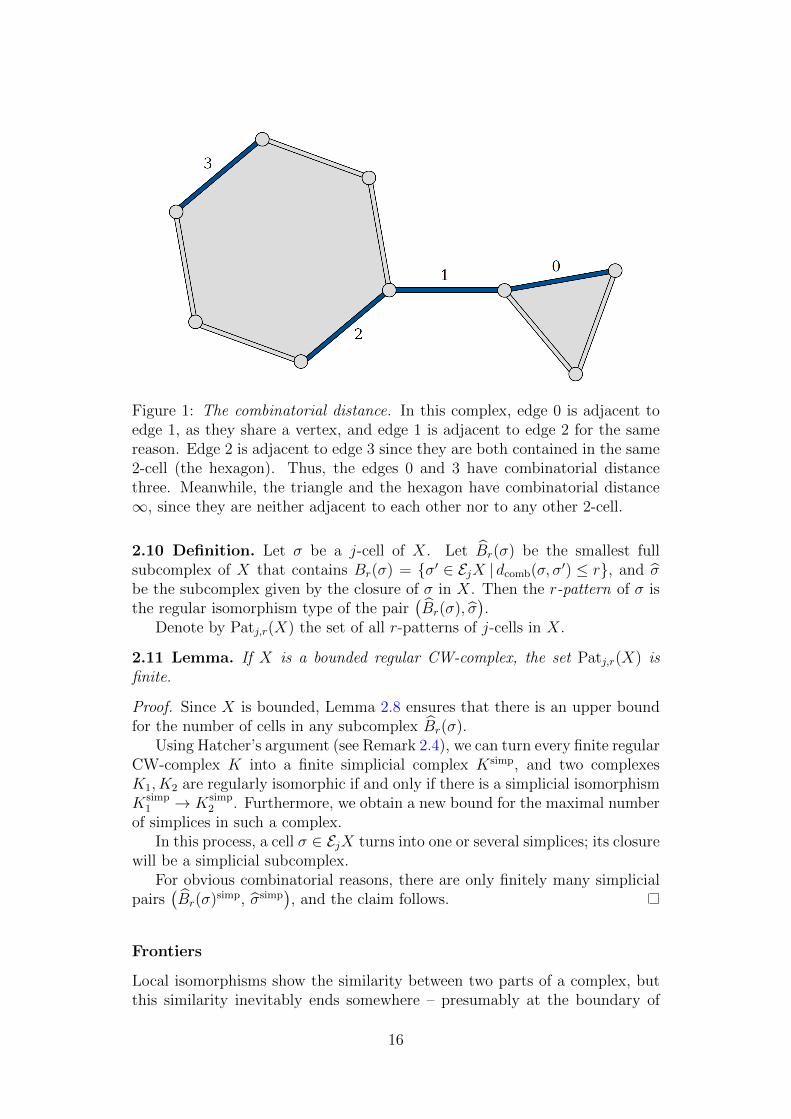
Figure 1: The combinatorial distance. In this complex, edge 0 is adjacent toedge 1, as they share a vertex, and edge 1 is adjacent to edge 2 for the samereason. Edge 2 is adjacent to edge 3 since they are both contained in the same2-cell (the hexagon). Thus, the edges 0 and 3 have combinatorial distancethree. Meanwhile, the triangle and the hexagon have combinatorial distance∞, since they are neither adjacent to each other nor to any other 2-cell.
2.10 Definition. Let σ be a j-cell of X. Let Br(σ) be the smallest fullsubcomplex of X that contains Br(σ) = σ′ ∈ EjX | dcomb(σ, σ′) ≤ r, and σbe the subcomplex given by the closure of σ in X. Then the r-pattern of σ isthe regular isomorphism type of the pair
(Br(σ), σ
).
Denote by Patj,r(X) the set of all r-patterns of j-cells in X.
2.11 Lemma. If X is a bounded regular CW-complex, the set Patj,r(X) isfinite.
Proof. Since X is bounded, Lemma 2.8 ensures that there is an upper boundfor the number of cells in any subcomplex Br(σ).
Using Hatcher’s argument (see Remark 2.4), we can turn every finite regularCW-complex K into a finite simplicial complex Ksimp, and two complexesK1, K2 are regularly isomorphic if and only if there is a simplicial isomorphismKsimp
1 → Ksimp2 . Furthermore, we obtain a new bound for the maximal number
of simplices in such a complex.In this process, a cell σ ∈ EjX turns into one or several simplices; its closure
will be a simplicial subcomplex.For obvious combinatorial reasons, there are only finitely many simplicial
pairs(Br(σ)simp, σsimp
), and the claim follows.
Frontiers
Local isomorphisms show the similarity between two parts of a complex, butthis similarity inevitably ends somewhere – presumably at the boundary of
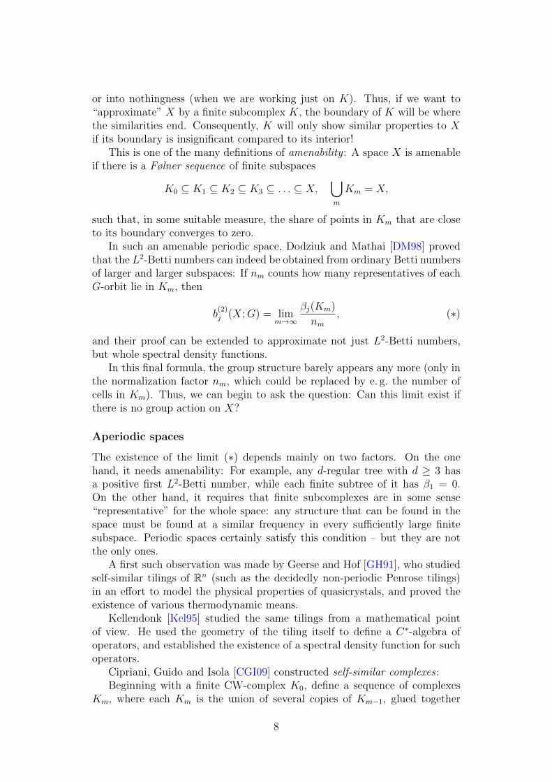
16
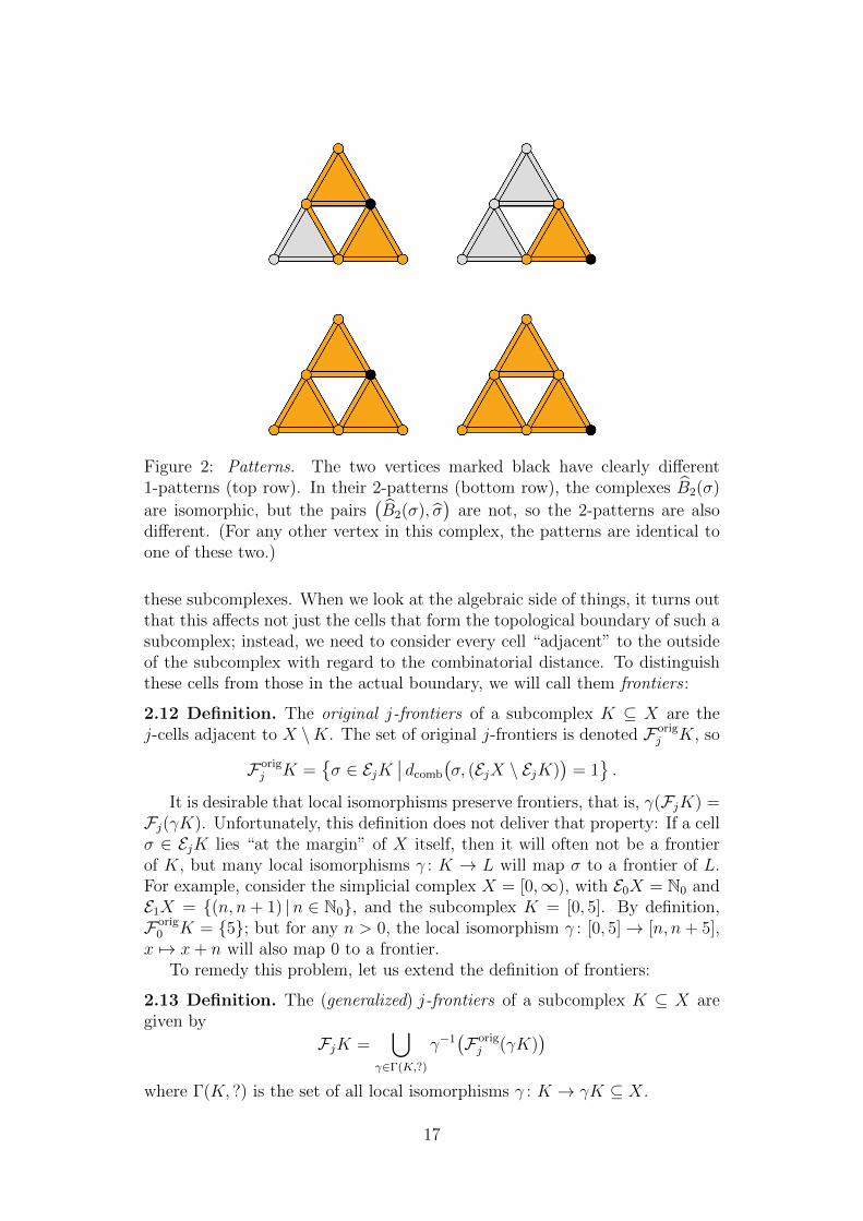
Figure 2: Patterns. The two vertices marked black have clearly different1-patterns (top row). In their 2-patterns (bottom row), the complexes B2(σ)
are isomorphic, but the pairs(B2(σ), σ
)are not, so the 2-patterns are also
different. (For any other vertex in this complex, the patterns are identical toone of these two.)
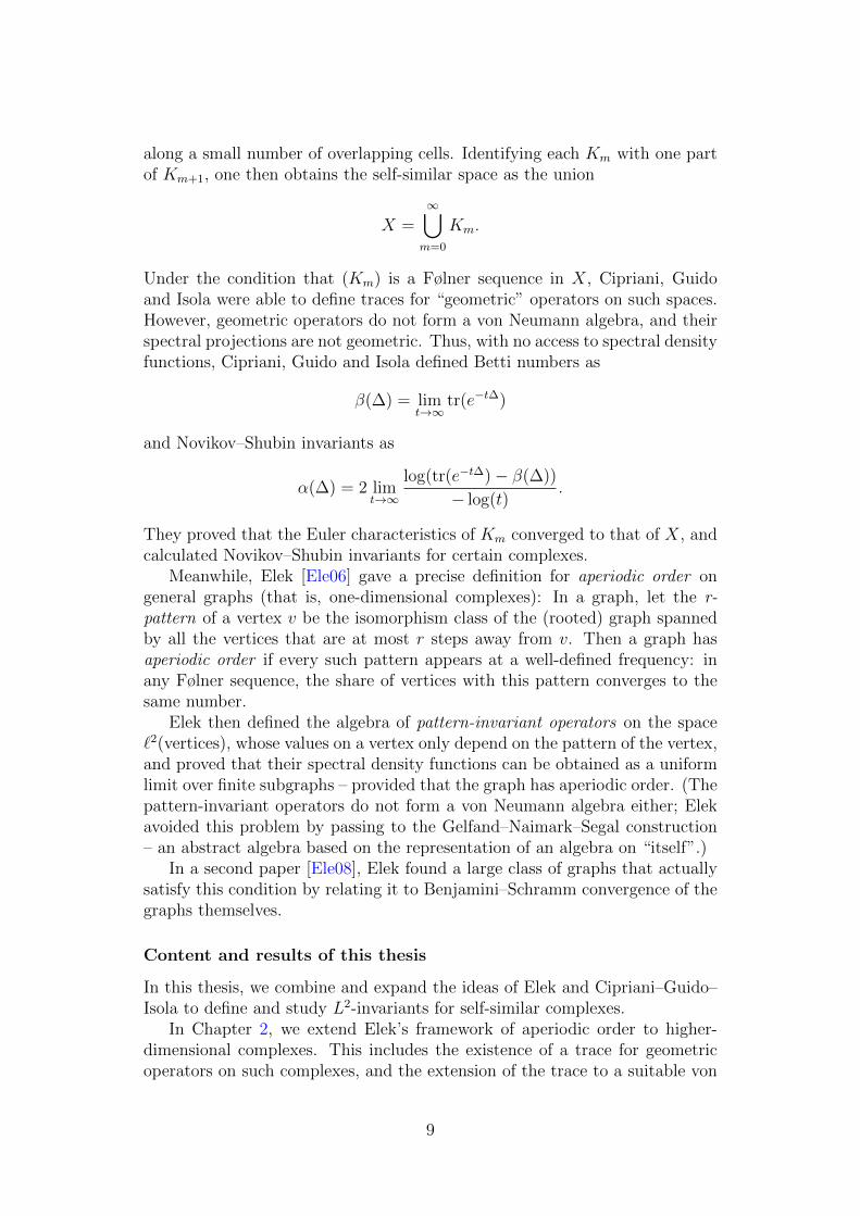
these subcomplexes. When we look at the algebraic side of things, it turns outthat this affects not just the cells that form the topological boundary of such asubcomplex; instead, we need to consider every cell “adjacent” to the outsideof the subcomplex with regard to the combinatorial distance. To distinguishthese cells from those in the actual boundary, we will call them frontiers :
2.12 Definition. The original j-frontiers of a subcomplex K ⊆ X are thej-cells adjacent to X \K. The set of original j-frontiers is denoted Forig
j K, so
Forigj K =
σ ∈ EjK
∣∣ dcomb
(σ, (EjX \ EjK)
)= 1.
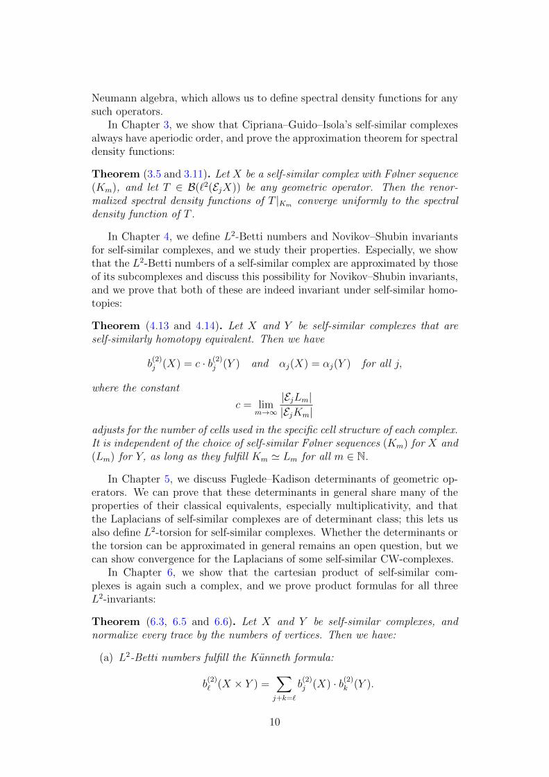
It is desirable that local isomorphisms preserve frontiers, that is, γ(FjK) =Fj(γK). Unfortunately, this definition does not deliver that property: If a cellσ ∈ EjK lies “at the margin” of X itself, then it will often not be a frontierof K, but many local isomorphisms γ : K → L will map σ to a frontier of L.For example, consider the simplicial complex X = [0,∞), with E0X = N0 andE1X = (n, n+ 1) |n ∈ N0, and the subcomplex K = [0, 5]. By definition,Forig
0 K = 5; but for any n > 0, the local isomorphism γ : [0, 5]→ [n, n+ 5],x 7→ x+ n will also map 0 to a frontier.
To remedy this problem, let us extend the definition of frontiers:
2.13 Definition. The (generalized) j-frontiers of a subcomplex K ⊆ X aregiven by
FjK =⋃
γ∈Γ(K,?)
γ−1(Forigj (γK)
)where Γ(K, ?) is the set of all local isomorphisms γ : K → γK ⊆ X.
17
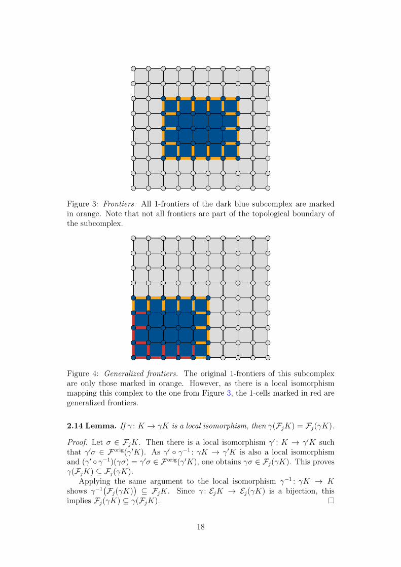
Figure 3: Frontiers. All 1-frontiers of the dark blue subcomplex are markedin orange. Note that not all frontiers are part of the topological boundary ofthe subcomplex.
Figure 4: Generalized frontiers. The original 1-frontiers of this subcomplexare only those marked in orange. However, as there is a local isomorphismmapping this complex to the one from Figure 3, the 1-cells marked in red aregeneralized frontiers.
2.14 Lemma. If γ : K → γK is a local isomorphism, then γ(FjK) = Fj(γK).
Proof. Let σ ∈ FjK. Then there is a local isomorphism γ′ : K → γ′K suchthat γ′σ ∈ Forig(γ′K). As γ′ γ−1 : γK → γ′K is also a local isomorphismand (γ′ γ−1)(γσ) = γ′σ ∈ Forig(γ′K), one obtains γσ ∈ Fj(γK). This provesγ(FjK) ⊆ Fj(γK).
Applying the same argument to the local isomorphism γ−1 : γK → Kshows γ−1
(Fj(γK)
)⊆ FjK. Since γ : EjK → Ej(γK) is a bijection, this
implies Fj(γK) ⊆ γ(FjK).
18
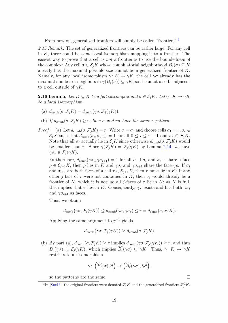
From now on, generalized frontiers will simply be called “frontiers”.3
2.15 Remark. The set of generalized frontiers can be rather large: For any cellin K, there could be some local isomorphism mapping it to a frontier. Theeasiest way to prove that a cell is not a frontier is to use the boundedness ofthe complex: Any cell σ ∈ EjK whose combinatorial neighborhood B1(σ) ⊆ Kalready has the maximal possible size cannot be a generalized frontier of K.Namely, for any local isomorphism γ : K → γK, the cell γσ already has themaximal number of neighbors in γ(B1(σ)) ⊆ γK, so it cannot also be adjacentto a cell outside of γK.
2.16 Lemma. Let K ⊆ X be a full subcomplex and σ ∈ EjK. Let γ : K → γKbe a local isomorphism.
(a) dcomb(σ,FjK) = dcomb(γσ,Fj(γK)).
(b) If dcomb(σ,FjK) ≥ r, then σ and γσ have the same r-pattern.
Proof. (a) Let dcomb(σ,FjK) = r. Write σ = σ0 and choose cells σ1, . . . , σr ∈EjX such that dcomb(σi, σi+1) = 1 for all 0 ≤ i ≤ r − 1 and σr ∈ FjK.Note that all σi actually lie in EjK since otherwise dcomb(σ,FjK) wouldbe smaller than r. Since γ(FjK) = Fj(γK) by Lemma 2.14, we haveγσr ∈ Fj(γK).
Furthermore, dcomb(γσi, γσi+1) = 1 for all i: If σi and σi+1 share a faceρ ∈ Ej−1X, then ρ lies in K and γσi and γσi+1 share the face γρ. If σiand σi+1 are both faces of a cell τ ∈ Ej+1X, then τ must lie in K: If anyother j-face of τ were not contained in K, then σi would already be afrontier of K, which it is not; so all j-faces of τ lie in K; as K is full,this implies that τ lies in K. Consequently, γτ exists and has both γσiand γσi+1 as faces.
Thus, we obtain
dcomb
(γσ,Fj(γK)
)≤ dcomb(γσ, γσr) ≤ r = dcomb(σ,FjK).
Applying the same argument to γ−1 yields
dcomb
(γσ,Fj(γK)
)≥ dcomb(σ,FjK).
(b) By part (a), dcomb(σ,FjK) ≥ r implies dcomb(γσ,Fj(γK)) ≥ r, and thus
Br(γσ) ⊆ Ej(γK), which implies Br(γσ) ⊆ γK. Thus, γ : K → γKrestricts to an isomorphism
γ :(Br(σ), σ
)→(Br(γσ), γσ
),
so the patterns are the same.
3In [Suc16], the original frontiers were denoted FjK and the generalized frontiers FGj K.
19
2.2 Aperiodic order and the trace
With the stage set, we can now begin to tame infinite complexes.
2.17 Definition. An amenable exhaustion or Følner sequence of a regularCW-complex X is a sequence of finite full subcomplexes Km ⊆ X such that
K1 ⊆ K2 ⊆ K3 ⊆ . . . ⊆ X and⋃m∈N
Km = X (exhaustion),
limm→∞
|FjKm||EjKm|
= 0 for all j with EjX 6= ∅ (amenability).
Note that if X is finite, then there must be an m0 ∈ N such that Km = X forall m ≥ m0.
The following definitions are a generalization of those given in [Ele06](where they were only used for graphs).
2.18 Definition. An (regular and bounded) CW-complex X has aperiodicorder if for every j, r ∈ N there is a function
Pj,r : Patj,r(X)→ [0, 1]
such that every amenable exhaustion (Km)m∈N satisfies
limm→∞
∣∣Eαj Km
∣∣|EjKm|
= Pj,r(α),
where Eαj Km is the set of cells σ ∈ EjKm whose r-patterns are equal to α ∈Patj,r(X).
Pj,r(α) is called the frequency of the pattern α. The definition immediatelyimplies ∑
α∈Patj,r(X)
Pj,r(α) = 1.
Note that if X is finite, then every amenable exhaustion is eventually con-stant, and the complex automatically has aperiodic order.
2.19 Example. The property that any amenable exhaustion produces thesame pattern frequencies is far from automatic. As a simple counterexample,define a CW-complex X as follows: Let E0X ∼= Z with 0-cells σn for n ∈ Z.Connect σn to σn+1 by one edge if n < 0, and by two edges if n ≥ 0:
· · · // σ−2// σ−1
// σ0**55 σ1
**55 σ2
**55 σ3
**44 · · ·
The 0-cells of this complex have three different 1-patterns: For σn with n < 0,the pattern is // • // , for σ0 it is // • ((
66 , and for σn withn > 0 it is ((
66 • ((66 .
20
For any positive integers a, b ∈ N, the full subcomplexes(K
[a,b]m
)m∈N spanned
by E0K[a,b]m = σn | −am ≤ n ≤ bm form an amenable exhaustion, and in that
exhaustion, we find the pattern frequencies
P[a,b]1,1 ( // • // ) = lim
m→∞
am− 1
am+ bm+ 1=
a
a+ b,
P[a,b]1,1 ( // • ((
66 ) = limm→∞
1
am+ bm+ 1= 0,
P[a,b]1,1 ( ((
66 • ((66 ) = lim
m→∞
bm− 1
am+ bm+ 1=
b
a+ b,
which clearly depend on the choice of the exhaustion. Thus, this complex doesnot have aperiodic order.
2.20 Definition. The propagation of an operator A ∈ B(`2(EjX)
)is given by
prop(A) = max dcomb(σ, σ′) |σ, σ′ ∈ EjX and 〈σ,Aσ′〉 6= 0 .
An operator A ∈ B(`2(EjX)
)is called r-pattern-invariant if prop(A) ≤ r
and the following commutativity condition holds: If γ : K → L is a localisomorphism and σ ∈ EjK such that Br(σ) ⊆ K and Br(γσ) ⊆ L, thenAγσ = γAσ and A∗γσ = γA∗σ.
An operator is called geometric if it is r-pattern-invariant for some r ∈ N.Denote by Ageo
j (X) the set of all geometric operators in B(`2(EjX)
).
2.21 Definition and Lemma. Let X be a regular and bounded CW-complex.
(a) For each j ∈ N0, let ∂j : `2(EjX) → `2(Ej−1X) be the operator inducedby the differential of the cellular chain complex of X.
That is, for any cells σ ∈ EjX and ρ ∈ Ej−1X, the value of 〈ρ, ∂jσ〉 isgiven by the degree of the map
Sj−1 fσ // X(j−1) proj // X(j−1)/(X(j−1) \ ρ
) ≈ // ρ/∂ρgρ // Sj−1,
where fσ is the attaching map of σ and gρ is induced by the inverse ofthe attaching map of ρ.
Each ∂j is a bounded operator.
(b) Define the j-th combinatorial Laplacian of X by
∆j = ∂j+1∂∗j+1 + ∂∗j ∂j.
Each ∆j is a positive 1-pattern-invariant operator on `2(EjX), and thusgeometric.
Proof. By definition of the combinatorial distance and Lemma 2.5, each ∆j
has propagation ≤ 1 and is indeed 1-pattern invariant. For a proof that ∂jand ∆j are bounded, see [Suc16], Lemma 2.2 / Def. 2.5 / Remark 2.6.
21
2.22 Lemma. Ageoj (X) is a ∗-algebra.
Proof. If A is r1-pattern-invariant and B is r2-pattern-invariant, then clearlyA+ cB is max(r1, r2)-pattern-invariant for every c ∈ C.
The composition AB is (r1 + r2)-pattern-invariant: Given γ : K → L andσ ∈ EjK such that Br1+r2(σ) ⊆ K and Br1+r2(γσ) ⊆ L, we can write Bσ =∑
σ′∈Br2 (σ) bσ′σ′ (since prop(B) ≤ r2) and thus obtain
ABγσ = AγBσ =∑
σ′∈Br2 (σ)
bσ′Aγσ′ =
∑σ′∈Br2 (σ)
bσ′γAσ′ = γABσ
using that for all σ′ ∈ Br2(σ) we have Br1(σ′) ⊆ Br1+r2(σ) ⊆ K and Br1(γσ
′) ⊆Br1+r2(γσ) ⊆ L. (The latter follows from Lemma 2.16.)
Finally, if A is r-pattern-invariant, then so is A∗; this follows directly fromthe definition.
2.23 Definition and Lemma. Let X be a complex with aperiodic order and(Km) an amenable exhaustion of X. Then the following defines a tracial stateon Ageo
j (X):
trA(T ) = limm→∞
1
|EjKm|∑
σ∈EjKm
〈σ, Tσ〉 (1)
This is independent of the choice of (Km), and if T ∈ Ageoj (X) is r-pattern-
invariant, then
trA(T ) =∑
α∈Patj,r(X)
Pr(α)〈σα, Tσα〉 , (2)
where σα ∈ EjX is any j-cell with r-pattern α.
Proof. Well-definedness: Let T ∈ Ageoj (X) be r-pattern-invariant. If two
j-cells ρ, σ ∈ EjX have the same r-pattern, then there is a local isomorphism
γ : Br(ρ)→ Br(σ) such that γρ = σ. Thus,
〈σ, Tσ〉 =〈γρ, Tγρ〉 =〈γρ, γTρ〉 =〈ρ, Tρ〉
because supp(Tρ) ⊆ Br(ρ). Therefore, 〈σ, Tσ〉 only depends on the r-patternof σ, and we obtain
1
|EjKm|∑
σ∈EjKm
〈σ, Tσ〉 =∑
α∈Patj,r(X)
∣∣Eαj Km
∣∣|EjKm|
〈σα, Tσα〉m→∞−−−→
∑α∈Patj,r(X)
Pr(α)〈σα, Tσα〉 .
This proves that the limit in Equation (1) exists and does not depend on thechoice of amenable exhaustion, and it proves Equation (2).
Linearity is clear from the definition.State: The Cauchy–Schwarz inequality and the convention ‖σ‖ = 1 yield
|〈σ, Tσ〉| ≤ ‖T‖ for all σ ∈ EjX, and thus |trA T | ≤ ‖T‖ for all T ∈ Ageoj (X).
Conversely, trA(id) = 1 = ‖id‖.
22
Trace property: Let S, T ∈ Ageoj (X) be r-pattern-invariant. (If S is r1-
pattern-invariant and T is r2-pattern-invariant, simply let r = max(r1, r2).)Define the the set of “r-frontiers” of Km
F rj Km = EjKm ∩Br−1(FjKm) =
σ ∈ EjKm
∣∣ dcomb
(σ, (EjX \ EjKm)
)≤ r.
Note that by boundedness of X there is C > 0 (depending on X and r, butnot on m) such that
∣∣F rj Km
∣∣ ≤ C |FjKm| for all m.∑σ∈EjKm
〈σ, STσ〉 =∑
σ∈EjKm\FrjKm
〈σ, STσ〉+O(|FjKm|)
=∑
σ∈EjKm\FrjKm
∑ρ∈EjKm
〈σ, Sρ〉〈ρ, Tσ〉+O(|FjKm|)
=∑
σ∈EjKm\FrjKm
∑ρ∈EjKm\FrjKm
〈σ, Sρ〉〈ρ, Tσ〉+O(|FjKm|)
In the first line, at most∣∣F r
j Km
∣∣ terms are left out; in the third line, at most
C∣∣F r
j Km
∣∣ terms are left out: For each ρ in F rj Km, there are at most C cells
σ for which 〈ρ, Tσ〉 6= 0. Each of the dropped terms is bounded by ‖S‖ ‖T‖.Thus, the O-constants depend on S and T , but not on m.
The same computation yields∑ρ∈EjKm
〈ρ, TSρ〉 =∑
ρ∈EjKm\FrjKm
∑σ∈EjKm\FrjKm
〈ρ, Tσ〉〈σ, Sρ〉+O(|FjKm|) .
Thus,1
|EjKm|∑
σ∈EjKm
〈σ, (ST − TS)σ〉 = O(|FjKm||EjKm|
)m→∞−−−→ 0.
2.3 The algebra of pattern-invariant operators
The ∗-algebra Ageoj (X) can easily be extended to a C∗-algebra:
2.24 Definition. Let Aj(X) be the operator-norm closure of Ageoj (X) in
B(`2(EjX)
). As the norm trA is norm-continuous, it immediately extends
to a trace on Aj(X).
This allows us to define a functional calculus f(T ) for every geometric op-erator T ∈ Ageo
j (X) and every continuous function f , and to take the tracetrA(f(T )). However, we are aiming to define spectral projections for these op-erators, that is, χ[0,λ](T ) with the clearly discontinuous characteristic functionsχ[0,λ]. This requires a von Neumann algebra!
The obvious next step would be to take the weak closure of Ageoj (X) in
B(`2(EjX)
), and extend the trace by weak continuity. Unfortunately, the
trace fails to be weakly continuous:
23
2.25 Example. Consider X = [0,∞) with the standard CW-structure givenby E0X = N0 and E1X = (n, n+ 1) |n ∈ N0. Here, every vertex has degreetwo, except for 0, which has degree one.
For each r ∈ N, define an operator Pr ∈ B(`2(E0X)) by
Prσ =
σ, if every vertex in Br(σ) has degree two,
0, otherwise.
Clearly, Pr is r-pattern-invariant and thus contained in Ageoj (X), and for every
r we have trA(Pr) = 1 because Prσ = σ for almost all σ ∈ E0X.But on the other hand, (Pr)r∈N is a decreasing sequence of projections that
weakly (even strongly) converge to zero! As trA(Pr)r→∞−−−→ 1 6= 0 = trA(0), the
trace is not weakly continuous.
To obtain a more suitable algebra, we employ the Gelfand–Naimark–Segalconstruction.
First of all, the trace on Aj(X) defines a scalar product on the algebraitself:
2.26 Definition. Define a hermitian form and the corresponding seminormon Aj(X) by
〈S, T 〉H = trA(S∗T ), ‖T‖H =√
trA(T ∗T ).
2.27 Lemma. Let S, T ∈ Aj(X). Then we have:
(a) ‖T‖H ≤ ‖T‖
(b) ‖T‖H = ‖T ∗‖H(c) ‖ST‖H ≤ ‖S‖ · ‖T‖H(d) ‖ST‖H ≤ ‖S‖H · ‖T‖
(e) The set Kj(X) = T ∈ Aj(X) | ‖T‖H = 0 is a closed ideal of Aj(X).
(f) Kj(X) = 0 if and only if for every r ∈ N and every σ ∈ EjX, ther-pattern of σ has positive frequency. Then, ‖ ‖H is a norm on Aj(X).
Proof. (a) This holds since trA is a state (and by the C∗-property):
‖T‖2H = trA(T ∗T ) ≤ ‖T ∗T‖ = ‖T‖2 .
(b) This follows directly from the trace property:
‖T‖2H = trA(T ∗T ) = trA(TT ∗) = ‖T ∗‖2
H .
(c) ‖ST‖2H = lim
m→∞
1
|EjKm|∑
σ ∈EjKm
‖STσ‖2 ≤ limm→∞
1
|EjKm|∑
σ ∈EjKm
‖S‖2 ‖Tσ‖2
= ‖S‖2 · ‖T‖2H.
24
(d) This follows from (b) and (c) combined.
(e) The triangle inequality for seminorms gives ‖S + λT‖H ≤ ‖S‖H+|λ| ‖T‖Hfor all λ ∈ C, so Kj(X) is a linear subspace. By (c), it is a left ideal,and by (d) it is a right ideal. Finally, it is closed (in the original normtopology) because trA and thus ‖ ‖H are norm-continuous.
(f) Assume there are a j-cell σ ∈ EjX and an r ∈ N such that the r-patternα of σ has Pj,r(α) = 0. Then the operator given by Tρ = ρ if ρ has thesame r-pattern as σ and Tρ = 0 otherwise is clearly r-pattern-invariantand non-zero, but its H-norm vanishes. Thus, Kj(X) is nontrivial.
Conversely, assume that every pattern of every j-cell in the complex haspositive frequency. Let T ∈ Aj(X) and σ ∈ EjX such that Tσ 6= 0. Bydefinition of Aj(X), there is S ∈ Ageo
j (X) such that ‖T − S‖ ≤ 13‖Tσ‖,
and S is s-pattern-invariant for some s ∈ N. Let ασ be the s-pattern ofσ. By assumption, Pj,s(ασ) > 0, and every ρ ∈ EjX with this patternfulfills
‖Sρ‖ = ‖Sσ‖ ≥ ‖Tσ‖ − ‖Tσ − Sσ‖ ≥ 2
3‖Tσ‖
=⇒ ‖Tρ‖ ≥ ‖Sρ‖ − ‖Sρ− Tρ‖ ≥ 1
3‖Tσ‖
This implies
‖T‖2H = trN (T ∗T ) ≥ Pj,s(ασ) ‖Tσ‖2
9> 0.
2.28 Remark. It should be noted that the H-norm is not submultiplicative:Consider a complex with just three cells, and let
T =
1 1 11 1 11 1 1
.
On Mat3(C), we have trA = 13
tr, and we obtain ‖T‖2H = 3 < 3
√3 = ‖T 2‖H.
With the newly constructed scalar product, we can complete Aj(X) into aHilbert space and have it act on this extended version of itself:
2.29 Definition and Lemma. Define a Hilbert space Hj(X) as the comple-tion of the pre-Hilbert space
(Aj(X)/Kj(X), 〈 , 〉H
).
Then the action of Aj(X) on Hj(X) by left multiplication yields a ∗-homo-morphism Aj(X) → B(Hj(X)). If Kj(X) = 0, this map is isometric (withrespect to the operator norms on each side).
Define the von Neumann algebra Nj(X) as the weak closure of Aj(X) inB(Hj(X)).
When the space X is clear, simply write Aj,Hj and Nj instead of Aj(X),Hj(X) and Nj(X).
25
Proof. Note first that the statements of Lemma 2.27 (b), (c) and (d) still holdif T (in (b) and (c)) respectively S (in (d)) are replaced by elements of Hj.This shows that for every T ∈ Aj, the map Hj → Hj,Ξ 7→ T ·Ξ is well-definedand has B(Hj)-operator norm less than or equal to ‖T‖. (In particular, if wechange the representative of Ξ by something of H-norm 0, then the result willalso change by something of H-norm 0.)
To see that Aj → B(Hj) is a ∗-homomorphism, note that for A,B, T ∈ Aj,
〈A, TB〉H = trA(A∗TB) = trA((T ∗A)∗B
)=〈T ∗A,B〉H ,
where T ∗ denotes the adjoint of T in Aj. Since Aj/Kj is dense in Hj (w.r.t.the H-norm), this proves 〈Ξ, TΥ〉H =〈T ∗Ξ,Υ〉H for all Ξ,Υ ∈ Hj, as desired.
Finally, if Kj = 0, then the map Aj → B(Hj) is injective (because id ∈ Hj,and T 6= 0 =⇒ T · id 6= 0), and every injective ∗-homomorphism betweenC∗-algebras is isometric.
2.30 Example. Let X be a finite complex, fix some j ∈ 0, . . . , dimX, andlet n = |EjX|. Then B(`2(EjX)) ∼= Matn(C), and the trace on Ageo
j (X) ⊆Matn(C) is given by the normalized matrix trace. The H-norm is given by thenormalized Frobenius norm
‖T‖H =
√√√√ 1
n
n∑i,j=1
|tij|2,
and obviously Kj(X) = 0. As the spaces are all finite-dimensional, all normsare equivalent, and we obtain Hj(X) = Aj(X) = Ageo
j (X). Furthermore,B(Hj) is finite-dimensional, and thus Aj(X) ⊆ B(Hj) is closed, so we alsoobtain Nj(X) = Aj(X) = Ageo
j (X).
2.31 Example. Let X = R with the standard CW-structure, so E0R ∼= Z ∼=E1R. In this case, every local isomorphism extends to a global isomorphism,and the group of global isomorphisms is generated by Z-translations and thereflection at zero.
Let us determine the geometric operators on E0R. Since they must beZ-equivariant, we can use the standard Fourier isomorphisms `2Z ∼= L2(S1)and B(`2Z)Z ∼= L∞(S1). Here, the reflection at zero corresponds to
R : L2(S1)→ L2(S1), f(z) 7→ f(z−1).
Thus, if a geometric operator T on `2(E0R) is given by a function t ∈ L∞(S1),that function must fulfill
t(z) · f(z−1) = TRf(z) = RTf(z) = (t · f)(z−1) = t(z−1) · f(z−1)
for any f ∈ L2(S1), and thus t(z) = t(z−1).On the other hand, a Z-equivariant operator of propagation r must be a
linear combination of shifts by distances ≤ r, so its corresponding function inL∞(S1) is a Laurent polynomial of degrees between −r and r.
26
Consequently, Ageo0 (R) corresponds to symmetric polynomials in z and z−1,
or equivalently, to polynomials in Re(z) = 12(z + z−1). By the Weierstrass
approximation theorem, the norm closure is given by
A0(R) ∼= C([−1, 1]).
The H-norm on A0 is clearly equivalent to the L2-norm on [−1, 1], and thus
H0(R) ∼= L2([−1, 1]),
which immediately implies
N0(R) ∼= L∞([−1, 1]).
In both examples, Nj can be identified with a linear subspace of Hj. Thisholds in general:
2.32 Lemma. The map Nj(X) → Hj(X), T 7→ T [id] is injective and hasdense image. Thus, Nj(X) can be identified with a dense subspace of Hj(X).
Proof. By Lemma 2.27 (d), right multiplication by an element of Aj is also abounded operator on Hj, and it certainly commutes with any operator givenby left multiplication with an element of Aj.
By the double commutant theorem, that means that right multiplicationby an element of Aj also commutes with every operator T ∈ Nj. Therefore, if[A] is the element of Hj represented by A ∈ Aj, we have
T [A] = T ([id] · A) = T [id] · A,
so the restriction of T to Aj/Kj ⊆ Hj is uniquely determined by the valueof T [id]. As Aj/Kj is dense in Hj, this implies that Nj → Hj, T 7→ T [id] isinjective. Finally, the image of this map certainly contains Aj/Kj, which isdense in Hj.
2.33 Corollary. The trace on Aj(X) extends to a weakly continuous faithfultrace on Nj, namely by
trN : Nj(X)→ C, T 7→〈[id], T [id]〉H .
Proof. The functional trN is by definition weakly continuous on B(Hj).For A ∈ Aj, we have
trN (A) =〈[id], A[id]〉H = trH(id∗A id) = trH(A) = trA(A),
so this indeed coincides with the original trace when applied to Aj.If P ∈ Nj is a non-zero projection, then
trN (P ) = trN (P ∗P ) =∥∥P [id]
∥∥2
H 6= 0
by Lemma 2.32. Thus, trN is faithful.
27
It remains to prove the trace property on Nj. Given S, T ∈ Nj, find nets(Ai)i∈I , (Bk)k∈K ⊆ Aj such that S = limi∈I Ai and T = limk∈K Bk in theweak operator topology. As trN is weakly continuous, multiplication is weaklycontinuous in each factor, and the trace property holds on Aj, we obtain
trN (ST ) = limi∈I
trN (AiT ) = limi∈I
limk∈K
trN (AiBk)
= limi∈I
limk∈K
trN (BkAi) = limi∈I
trN (TAi) = trN (TS).
2.34 Remark. For completeness, let us show that the mapNj → Hj, T 7→ T [id]is in general not surjective. One such example is given in 2.31, where we showNj ∼= L∞([−1, 1]) $ L2([−1, 1]) ∼= Hj.
Here is a second example: Assume that in the complex X there are patternsαn ∈ Patrn,j(X), with 0 = r0 < r1 < r2 < . . ., such that each σ ∈ EjX withrn-pattern αn also has rm-pattern αm for all m ≤ n, but only half of these cellsalso have rn+1-pattern αn+1. Then αn has frequency 2−n. Now define An ∈ Ajby
Anσ = 2m/3σ, where m = min (n, max k |σ has rk-pattern αk) .
This is a Cauchy sequence in H:
‖An − Am‖2H = trH
((An − Am)2
)=
n∑k=m+1
2−(k+1) ·(2k/3 − 2m/3
)2+
∞∑k=n+1
2−(k+1) ·(2n/3 − 2m/3
)2
≤n∑
k=m+1
2−(k+1) · 22k/3 +∞∑
k=n+1
2−(k+1) · 22n/3
=n∑
k=m+1
2−k/3−1 + 2−(n+1) · 22n/3
≤ 1
2
∞∑k=m+1
2−k/3 + 2−n/3−1 m,n→∞−−−−→ 0.
Thus, Ξ = limn→∞An exists in Hj. Assume that there were T ∈ Nj such thatT [id] = Ξ. Then, by the argument from the proof of Lemma 2.32, we wouldhave T [Am] = T [id] ·Am = Ξ ·Am for every m ∈ N. Since T is by assumptioncontinuous, this gives TΞ = limm→∞ Ξ·Am. Conversely, as right multiplicationby Am is continuous, Ξ · Am = limn→∞An · Am.
For all m ≤ n, we have
‖AmAn‖2H = trH(AnA
2mAn)
≥ trH(A4m) =
m∑k=0
2−(k+1) · 24k/3 + 2−(m+1) · 24m/3
=m∑k=0
2k/3−1 + 2m/3−1 m→∞−−−→ ∞.
Thus, TΞ cannot be an element of Hj. Contradiction!
28
2.4 Dimensions
In the finite-dimensional world, every dimension of a vector space can be ex-pressed as the trace of the projection to that space. With the trace on Nj(X)developed above, we can apply the same concept to define finite dimensionsfor certain subspaces of Hj(X):
2.35 Definition. A closed subspace V ⊆ Hj(X) is called geometric, if theorthogonal projection to V lies in Nj(X). For every such subspace, definedimN (V ) = trN (projV ).
Let us collect some basic properties of this dimension:
2.36 Lemma. (a) If V,W ⊆ Hj(X) are geometric subspaces, then so areV ⊥, V ∩W and V +W .
(b) If V ⊥ W , then dimN (V ⊕W ) = dimN (V ) + dimN (W ).
(c) If T ∈ Nj(X), then ker(T ) and im(T ) are geometric subspaces, and
dimN(im(T )
)= dimN
(Hj(X)
)− dimN
(ker(T )
).
(d) If V,W ⊆ Hj(X) are geometric subspaces, then
dimN (V +W ) = dimN (V ) + dimN (W )− dimN (V ∩W ).
Proof. (a) If PV is the orthogonal projection to V ∈ Nj(X), then id − PV ∈Nj(X) projects to V ⊥, so V ⊥ is geometric.
By a theorem of von Neumann [von50], the projection to V ∩W is givenby
PV ∩W = limn→∞
(PV PW )n
in strong operator topology. This is clearly contained in Nj(X), so V ∩W isgeometric.
Since (V + W )⊥ = V ⊥ ∩W⊥, the third statement follows from the firsttwo.
(b) This follows directly from PV⊕W = PV + PW .(c) Since χ0(T ) ∈ Nj(X) projects to ker(T ), the kernel is geometric, and
as im(T ) = ker(T ∗)⊥, it follows from (a) that im(T ) is also geometric.Write T = U |T | with |T | =
√T ∗T and U unitary. Clearly, U, |T | ∈ Nj(X)
and ker(T ) = ker |T |. If Q projects to im |T |, then UQU∗ projects to im(T ),so we get
dimN(ker(T )
)= dimN
(ker |T |
), dimN
(im(T )
)= dimN
(im |T |
).
Finally, as |T | is self-adjoint, we have
Hj(X) = ker |T | ⊕ im |T |,
so the statement follows from (b).
29
(d) Let W = (id − PV )W be the projection of W to V ⊥. This gives the
orthogonal decomposition V + W = V ⊕ W , and by (b), dimN (V + W ) =
dimN (V ) + dimN (W ). Note that W is geometric by (c), because it is theimage of (id−PV )PW . Furthermore, ker
((id−PV )PW
)= W⊥⊕ (V ∩W ), and
so (b) and (c) yield
dim W = dimN(
im((id− PV )PW ))
= dimN(Hj(X)
)− dimN (W⊥)− dimN (V ∩W )
= dimN (W )− dimN (V ∩W )
This completes the proof.
2.37 Corollary. If V,W ⊆ Hj(X) are two geometric subspaces such thatdimN (V ) < dimN (W ), then W ∩ V ⊥ 6= 0.
Proof. Apply Lemma 2.36 to PV PW . We have ker(PV PW ) = W⊥⊕ (W ∩V ⊥),and im(PV PW ) ⊆ V . Therefore,
dimN (V ) ≥ dimN(im(PV PW )
)= dimN
(Hj(X)
)− dimN
(W⊥)− dimN
(W ∩ V ⊥
)= dimN (W )− dimN
(W ∩ V ⊥
)=⇒ dimN
(W ∩ V ⊥
)≥ dimN (W )− dimN (V ) > 0.
As a zero space would have dimension zero, this completes the proof.
2.5 Spectral density functions
We are now, finally, ready to define and discuss the spectral density functions(or “integrated densities of states”) of geometric operators:
2.38 Definition. Given a positive operator T ∈ Nj(X) and λ ∈ [0,∞), definethe spectral projections of T by
ET (λ) = χ(−∞,λ](T ) = χ[0,λ](T ) ∈ Nj(X)
and the spectral density function of T by
F T : [0,∞)→ [0, 1], λ 7→ trN(ET (λ)
).
In general, for any operator T ∈ Nj(X), define
ET (λ) = ET ∗T (λ2) and F T (λ) = F T ∗T (λ2).
(This is well-defined, as Lemma A.8 proves the equality ET (λ) = ET ∗T (λ2) forself-adjoint T .)
30
2.39 Lemma. Let T ∈ Nj. Then its spectral density function F T fulfills thefollowing:
(a) F T (0) = dimN (ker T ).
(b) F T is increasing.
(c) F T is right-continuous.
(d) F T (λ) = dimN (Hj) = 1 for every λ ≥ ‖T‖.Proof. All of this follows from the definition and Theorem A.6.
2.40 Lemma. For any T ∈ Nj(X) and all λ ≥ 0, we have F T (λ) = F |T |(λ) =F T ∗(λ).
Proof. By definition,
F T (λ) = trN ET ∗T (λ) = trN E
|T |2(λ) = F |T |(λ)
and F T ∗(λ) = trN ETT ∗(λ). Since spec(T ∗T ) ⊆ [0,∞), we have ET ∗T (λ) =
χ[0,λ](T∗T ) and the same for TT ∗. Choose a sequence of polynomials (pm)m∈N
that converge pointwise to χ[0,λ]. Then Theorem A.3 implies that pm(T ∗T )converges weakly to ET ∗T (λ), and as the trace is weakly continuous, we getF T (λ) = limm→∞ trN pm(T ∗T ) and F T ∗(λ) = limm→∞ trN pm(TT ∗).
On the other hand, the trace property implies trN((T ∗T )k
)= trN
((TT ∗)k
)for all k, so (by linearity of the trace) those two limits are equal.
2.41 Remark. If EjX is finite, every self-adjoint operator T ∈ Nj(X) cor-responds to a hermitian (n × n)-matrix, and there is an orthonormal basisof Cn with respect to which T has the form diag(λ1, . . . , λn) with eigenvaluesλ1 ≤ . . . ≤ λn. Then the spectral projection ET (µ) is given by the projectionto the first k basis vectors, where k is given by λk ≤ µ < λk+1, and F T (µ) =trN (ET (µ)) = k/n. Especially, the spectral density function of an operator ona finite-dimensional space is always a right-continuous step function.
The idea of spectral density functions is that F (λ) measures the size of themaximal subspace on which T is bounded by λ:
2.42 Lemma. Let T ∈ Nj(X) be self-adjoint and µ ≥ 0. Then
F T (µ) = max dimN V |V ⊆ Hj(X) geometric, ‖T |V ‖ ≤ µ .
(Here, T |V is considered as an operator T : V → Hj(X).)
Proof. By definition, F T (µ) = trN (ET (µ)) = dimN(imET (µ)
), and the space
imET (µ) is geometric. Lemma A.9 gives ‖Tv‖ ≤ µ ‖v‖ for all v ∈ imET (µ),and thus
F T (µ) = dimN (imET (µ)) ≤ max dimN V |V geometric, ‖T |V ‖ ≤ µ .
Conversely, let V ⊆ `2(EjX) be a geometric subspace such that dimN V >F T (µ). By Corollary 2.37, this implies that there is a nonzero vector x ∈V ∩
(imET (µ)
)⊥. Then, Lemma A.9 yields ‖Tx‖ > µ ‖x‖, and therefore
‖T |V ‖ > λ.
31
Finally, it should be noted that the spectral density function of an operatorT contains all necessary information to determine the trace for any operatorthat can be obtained from T through functional calculus:
2.43 Lemma. For any self-adjoint T ∈ N (X) and any function f ∈ L∞(R),we have
trN(f(T )
)=
∫Rf(λ) dF T (λ),
where the measure dF T (λ) is given by dF T((a, b]
)= F T (b)− F T (a).
Proof. Using the definition of F and Theorem A.6, we obtain:
trN(f(T )
)=〈[idX ], f(T )[idX ]〉H =
∫Rf(λ) d
⟨[idX ], ET (λ)[idX ]
⟩H
=
∫Rf(λ) d
(trN(ET (λ)
))=
∫Rf(λ) dF T (λ).
2.44 Remark. If one is interested solely in the spectral density functions ofgeometric operators, but not in their von Neumann algebra, Lemma 2.43 canserve as an alternative definition:
For any bounded continuous function f : spec(T )→ C, we have f(T ) ∈ Aj,so trA(f(T )) is immediately defined. Especially, this defines a positive linearfunctional
Cc(spec(T ))→ C, f 7→ trA(f(T )).
By the Riesz–Markov–Kakutani representation theorem (see [Els11], p. 358),this implies the existence of a unique locally finite inner regular measure µT
on spec(T ) such that
trN(f(T )
)=
∫spec(T )
f dµT
holds for every f ∈ Cc(spec(T )). One can then define the spectral densityfunction by
F T (λ) =
∫spec(T )
χ[0,λ] dµT ,
obtaining the same function as in our Definition 2.38 (and, of course, dF T =µT ). The author would like to thank Ralf Meyer for pointing out this approach.
32
3 Self-similar complexes and uniform conver-
gence
In the previous chapter, we have been using spaces with aperiodic order , thatis, spaces where every pattern of cells appears at a frequency that becomesapproximately constant on a large scale. Now, we shall discuss a way toactually construct such spaces using self-similarity.
In short, a self-similar space is obtained through an iterative process: Westart with a finite cell complex and glue several copies of it together. We canthen use the resulting (still finite) complex and repeat the process ad infinitum,eventually obtaining the self-similar complex as the union of all iteration steps.
It is intuitively clear that patterns that are present in the finite subcom-plexes will repeat infinitely often in the final complex. On the other hand,whenever two subcomplexes are glued together, new patterns can be created.This lets the whole complex be more than the sum of its parts, but it also holdspotential for instability and divergence. To keep this variation in check, weneed amenability : The number of cells at which different subcomplexes meeteach other must be small compared to the total number of cells.
Under these conditions, we will show first that the self-similar structureindeed implies the aperiodic order required in the previous chapter. Then,we will come to the centerpiece of this thesis: We will prove that, on a self-similar complex, the spectral density function for any geometric operator canbe approximated uniformly by the spectral density functions of the finite sub-complexes that form the self-similar structure.
3.1 Definition. A self-similar complex is a bounded regular CW-complex Xfor which there is a self-similar exhaustion, that is, an amenable exhaustionK1 ⊆ K2 ⊆ K3 ⊆ . . . ⊆ X by connected4 subcomplexes as in Def. 2.17, suchthat for each m ∈ N there is a finite set G(m,m + 1) of local isomorphismsγ : Km → γKm ⊆ X that fulfills
Km+1 =⋃
γ∈G(m,m+1)
γKm,
Ej(γ1Km) ∩ Ej(γ2Km) = Fj(γ1Km) ∩ Fj(γ2Km) for all γ1 6= γ2.
Thus, each subcomplex Km+1 consists of “copies” of the next-smaller subcom-plex Km that overlap only at their frontiers. Write
G(m,m+ k) = γm+k−1 . . . γm+1 γm | γj ∈ G(j, j + 1) ,
G(m) =∞⋃k=0
G(m,m+ k).
4Connectedness in the topological sense implies that any two vertices in Km have a finitecombinatorial distance; this is relevant for the proof of Theorem 3.4. On the other hand, itdoes not imply that any two j-cells for j ≥ 2 have finite combinatorial distance, and that isnot needed for any proofs.
33
Then we obtain
Km+k =⋃
γ∈G(m,m+k)
γKm and X =⋃
γ∈G(m)
γKm,
where the various copies of Km still only overlap at their frontiers.
Note that the self-similar exhaustion (Km) and its local isomorphism setsG(m,m+ 1) are not a fixed part of the structure – they only need to exist.
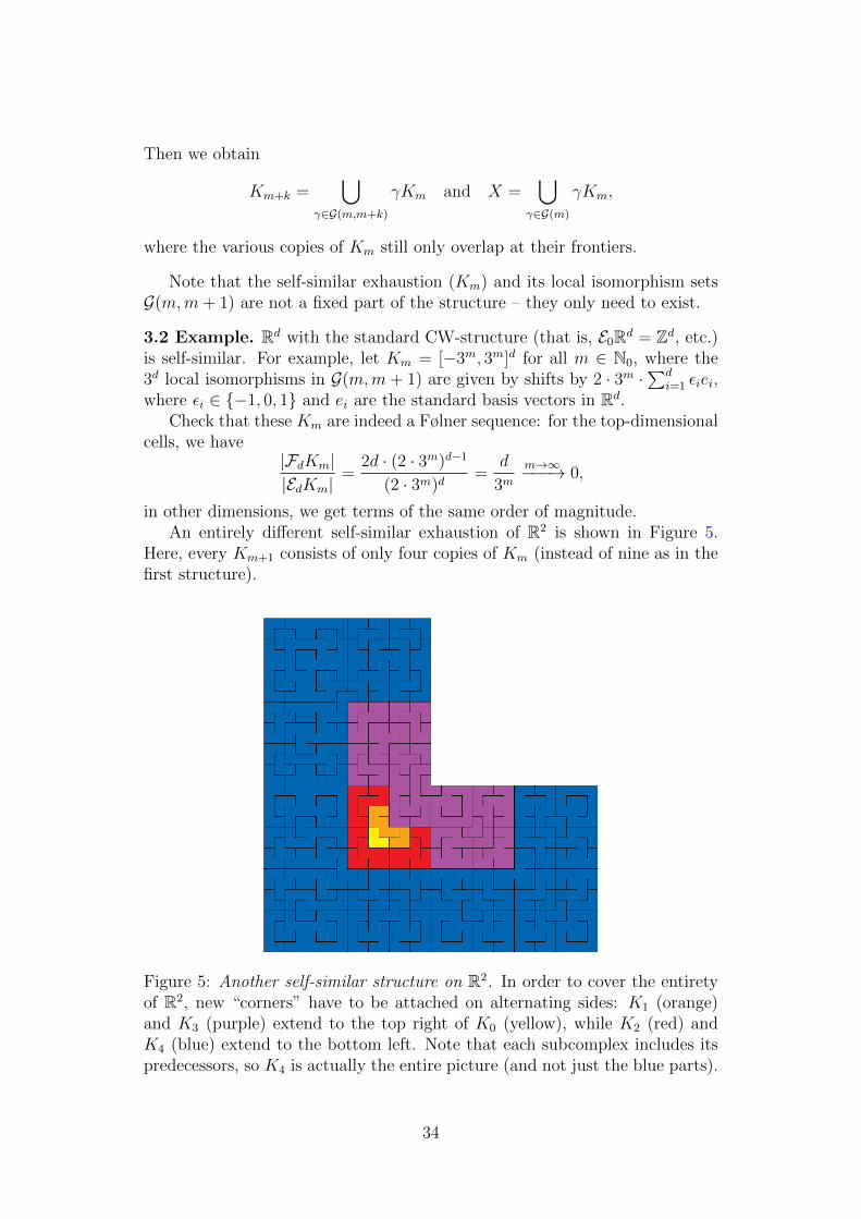
3.2 Example. Rd with the standard CW-structure (that is, E0Rd = Zd, etc.)is self-similar. For example, let Km = [−3m, 3m]d for all m ∈ N0, where the3d local isomorphisms in G(m,m + 1) are given by shifts by 2 · 3m ·
∑di=1 εiei,
where εi ∈ −1, 0, 1 and ei are the standard basis vectors in Rd.Check that these Km are indeed a Følner sequence: for the top-dimensional
cells, we have|FdKm||EdKm|
=2d · (2 · 3m)d−1
(2 · 3m)d=
d
3mm→∞−−−→ 0,
in other dimensions, we get terms of the same order of magnitude.An entirely different self-similar exhaustion of R2 is shown in Figure 5.
Here, every Km+1 consists of only four copies of Km (instead of nine as in thefirst structure).
Figure 5: Another self-similar structure on R2. In order to cover the entiretyof R2, new “corners” have to be attached on alternating sides: K1 (orange)and K3 (purple) extend to the top right of K0 (yellow), while K2 (red) andK4 (blue) extend to the bottom left. Note that each subcomplex includes itspredecessors, so K4 is actually the entire picture (and not just the blue parts).
34
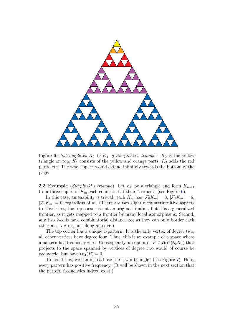
Figure 6: Subcomplexes K0 to K4 of Sierpinski’s triangle. K0 is the yellowtriangle on top, K1 consists of the yellow and orange parts, K2 adds the redparts, etc. The whole space would extend infinitely towards the bottom of thepage.
3.3 Example (Sierpinski’s triangle). Let K0 be a triangle and form Km+1
from three copies of Km each connected at their “corners” (see Figure 6).In this case, amenability is trivial: each Km has |F0Km| = 3, |F1Km| = 6,
|F2Km| = 0, regardless of m. (There are two slightly counterintuitive aspectsto this: First, the top corner is not an original frontier, but it is a generalizedfrontier, as it gets mapped to a frontier by many local isomorphisms. Second,any two 2-cells have combinatorial distance ∞, as they can only border eachother at a vertex, not along an edge.)
The top corner has a unique 1-pattern: It is the only vertex of degree two,all other vertices have degree four. Thus, this is an example of a space wherea pattern has frequency zero. Consequently, an operator P ∈ B(`2(E0X)) thatprojects to the space spanned by vertices of degree two would of course begeometric, but have trA(P ) = 0.
To avoid this, we can instead use the “twin triangle” (see Figure 7). Here,every pattern has positive frequency. (It will be shown in the next section thatthe pattern frequencies indeed exist.)
35
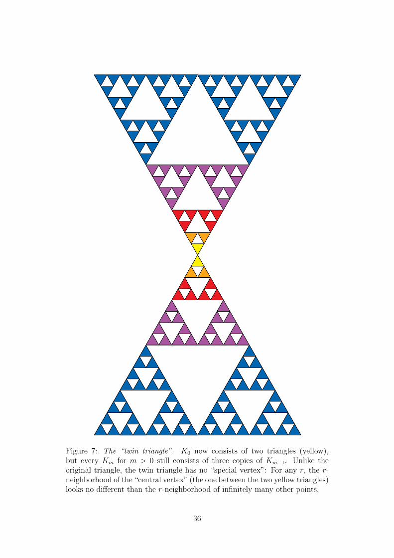
Figure 7: The “twin triangle”. K0 now consists of two triangles (yellow),but every Km for m > 0 still consists of three copies of Km−1. Unlike theoriginal triangle, the twin triangle has no “special vertex”: For any r, the r-neighborhood of the “central vertex” (the one between the two yellow triangles)looks no different than the r-neighborhood of infinitely many other points.
36
3.1 Self-similarity implies aperiodic order
Let us now prove that self-similar complexes do indeed have aperiodic order.This is not surprising, as their construction has clearly a “repetitive” nature,but it is not completely obvious either, since we need to check that the fre-quency of patterns converges not just along a given self-similar exhaustion, butalong any Følner sequence, self-similar or not.
3.4 Theorem. Every self-similar complex has aperiodic order.
Proof. Let (Km) be a self-similar exhaustion of X. Fix j, r ∈ N0 and a patternα ∈ Patj,r(X).
For any subcomplex K ⊆ X, consider the “r-interior”:
IrjK = σ ∈ EjK | dcomb(σ,X \K) > r ,Ir,αj K =
σ ∈ IrjK
∣∣σ has r-pattern α.
By Lemma 2.16, we have
∣∣Ir,αj (γKm)∣∣ =
∣∣Ir,αj Km
∣∣ for every γ ∈ G(m,n),
Irj (γ1Km) ∩ Irj (γ2Km) = ∅ whenever γ1, γ2 ∈ G(m,n) with γ1 6= γ2,
∣∣∣∣EjKn \⊔
γ ∈G(m,n)
Irj (γKm)
∣∣∣∣ ≤ Cr |G(m,n)| |FjKm|,
where Cr = maxσ ∈EjX
|Br(σ)|. (Cr is finite since X is bounded.)
Therefore, the number of times the pattern α appears in Kn is given by∣∣Eαj Kn
∣∣ =∑
γ ∈G(m,n)
∣∣Ir,αj (γKm)∣∣+O(|G(m,n)| |FjKm|)
= |G(m,n)|∣∣Ir,αj Km
∣∣+O(|G(m,n)| |FjKm|)= |G(m,n)|
∣∣Eαj Km
∣∣+O(|G(m,n)| |FjKm|)
where the last line follows from |EjKm| −∣∣IrjKm
∣∣ ≤ Cr |FjKm|.On the other hand, the total number of j-cells in Kn is
|EjKn| =∑
γ ∈G(m,n)
∣∣I1j (γKm)
∣∣+O(|G(m,n)| |FjKm|)
= |G(m,n)|∣∣I1jKm
∣∣+O(|G(m,n)| |FjKm|)= |G(m,n)| |EjKm|+O(|G(m,n)| |FjKm|)
One obtains the pattern frequency:∣∣Eαj Kn
∣∣|EjKn|
=|G(m,n)|
∣∣Eαj Km
∣∣+O(|G(m,n)| |FjKm|)|G(m,n)| |EjKm|+O(|G(m,n)| |FjKm|)
=
∣∣Eαj Km
∣∣+O(|FjKm|)|EjKm|+O(|FjKm|)
37
Now fix any ε > 0. Choose m large enough that for all n ≥ m, the O-termsare less than ε |EjKm|, which gives:
1− ε1 + ε
∣∣Eαj Km
∣∣|EjKm|
≤∣∣Eαj Kn
∣∣|EjKn|
≤ 1 + ε
1− ε
∣∣Eαj Km
∣∣|EjKm|
Thus, the sequence of frequencies( |Eαj Km||EjKm|
)is convergent, and it has a limit
Pj,r(α) = limm→∞
∣∣Eαj Km
∣∣|EjKm|
.
It remains to show that if (Lk) is a different amenable exhaustion of X,
then( |Eαj Lk||EjLk|
)converges to the same limit.
Again, fix ε > 0. LetCr = max
σ ∈EjX|Br(σ)| .
Choose m large enough that∣∣∣∣∣Pj,r(α)−∣∣Eαj Km
∣∣|EjKm|
∣∣∣∣∣ ,∣∣∣∣∣Pj,r(α)−
∣∣I1,αj Km
∣∣|EjKm|
∣∣∣∣∣ andCr |FjKm||EjKm|
are all smaller than ε.Let5
bm = maxρ,ρ′ ∈E0Km
dcomb(ρ, ρ′)
(note that this is always finite) and
Dm = maxρ∈E0X
|Bbm(ρ)| .
Then choose k0 large enough such that for all k ≥ k0,
|FjLk||EjLk|
<ε
Dm
.
For m ∈ N, let
Gin(m, k) = γ ∈ G(m) | γKm ⊆ Lk ,Gout(m, k) = γ ∈ G(m) | γKm ∩ Lk 6= ∅ ,Gfront(m, k) = Gout(m, k) \ Gin(m, k).
Then the frequency of the pattern α in Lk can be estimated by
|Gin(m, k)|∣∣I1,αj Km
∣∣|Gout(m, k)| |EjKm|
≤∣∣Eαj Lk∣∣|EjLk|
≤|Gout(m, k)|
(∣∣Eαj Km
∣∣+ Cr |FjKm|)
|Gin(m, k)|∣∣I1jKm
∣∣5Unlike Cr, which counts the j-cells in r-patterns, the constant Dm always counts 0-cells.
This is necessary because we will soon use that any two 0-cells in the complex are connectedby a “path” of adjacent cells, which does not hold for general j-cells.
38
where the term |Gout(m, k)|Cr |FjKm| estimates the number of cells whoser-pattern in Lk may stretch across multiple copies of Km.
By choice of m, we already know
(1− ε)Pj,r(α) ≤∣∣I1,αj Km
∣∣|EjKm|
and
∣∣Eαj Km
∣∣+ Cr |FjKm|∣∣I1jKm
∣∣ ≤ 1 + 2ε
1− εPj,r(α).
It remains to bound the ratio of |Gin(m, k)| and |Gout(m, k)|.If γ ∈ Gfront(m, k), then γKm contains a vertex in Lk and a vertex in
X \ Lk; since Km (and thus γKm) is connected, it must also contain a vertexρ ∈ F0Lk. Therefore, ⋃
γ ∈Gfront(m,k)
E0(γKm) ⊆ Bbm(F0Lk)
and thus ∣∣∣∣∣∣⋃
γ ∈Gfront(m,k)
E0(γKm)
∣∣∣∣∣∣ ≤ Dm |F0Lk| .
Conversely, as the different copies of Km only overlap at their frontiers, wehave
|Gfront(m, k)| · (|E0Km| − |F0Km|) ≤
∣∣∣∣∣∣⋃
γ ∈Gfront(m,k)
E0(γKm)
∣∣∣∣∣∣ .Combining the previous two equations yields the estimate
|Gfront(m, k)| · (|E0Km| − |F0Km|) ≤ Dm |F0Lk| ,
and if m is large enough to ensure |F0Km| ≤ 12|E0Km|, we obtain
|Gfront(m, k)| ≤ Dm |F0Lk||E0Km| − |F0Km|
≤ 2Dm|F0Lk||E0Km|
On the other hand,
Lk ⊆⋃
γ ∈Gout(m,k)
γKm =⇒ |Gout(m, k)| ≥ |E0Lk||E0Km|
,
which implies|Gfront(m, k)||Gout(m, k)|
≤ 2Dm|F0Lk||E0Lk|
< 2ε
and therefore|Gin(m, k)||Gout(m, k)|
≥ 1− 2ε.
Thus, we finally end up with
(1− 2ε)(1− ε)Pj,r(α) ≤∣∣Eαj Lk∣∣|EjLk|
≤ 1 + ε
(1− 2ε)(1− ε)Pj,r(α).
As ε was arbitrary and this holds for all k ≥ k0, the limits indeed coincide.
39
3.2 Approximating spectral density functions
We now come to the main theorem about spectral density functions of geo-metric operators on self-similar complexes.
Given any geometric operator T on a self-similar complex X, we form asequence of “restricted” operators Tm on the finite subcomplexes Km.6
These operators Tm can always be obtained by Tm := PmTIm, whereIm : `2(EjKm) → `2(EjX) is the inclusion and Pm : `2(EjX) → `2(EjKm) isthe orthogonal projection.
However, as the proof of convergence extensively uses that the frontiersof Km are negligible compared to its interior, the behavior of Tm near thesefrontiers is equally negligible. Thus, our choice of Tm is rather flexible. In themost interesting case, when T = ∆
(X)j is the Laplacian on X, we can choose
Tm = ∆(Km)j to be the Laplacian on Km (which ignores the existence of all
cells in X \ Km), even if that operator takes significantly different values onfrontiers of Km.
Firstly, in Theorem 3.5, we will show that the spectral density functions ofthe operators Tm are uniformly convergent (without yet specifying the limit).Then, in Theorem 3.11, we will show that their limit is actually the spectraldensity function of T as defined in Def. 2.38.
This is remarkable in so far as the function from 2.38 measured the sizesof subspaces of Hj(X) (the abstract Hilbert space formed from the geometricoperators themselves), while the spectral density functions of the Tm actuallymeasure subspaces spanned by cells in Km. Furthermore, it proves that thechoice of (Km) does not matter at all – the spectral density functions willalways converge to the same limit!
3.5 Theorem. Let X be a self-similar CW-complex with self-similar exhaus-tion (Km)m∈N, and let T ∈ Ageo
j (X) be a positive r-pattern-invariant operator.Choose a sequence of positive operators Tm ∈ B(`2(EjKm)) such that, for
all m, ‖Tm‖ ≤ C for some constant C, prop(Tm) ≤ r, and Tσ = Tmσ forevery σ ∈ Ir+1
j Km.Let Fm be the spectral density functions of Tm, that is,
Fm(λ) =1
|EjKm|max
dimCW
∣∣∣∣W ⊆ `2(EjKm) linear subspace such that
‖Tmv‖ ≤ λ · ‖v‖ for all w ∈ W
.
Then the sequence of functions Fm converges uniformly, and the limit does notdepend on the choice of the sequence (Tm).
Before we begin the actual proof, some elementary lemmas:
3.6 Lemma. Let A,B be finite-dimensional vector spaces and C ⊆ A⊕ B bea subspace. Then
dim(A ∩ C) ≥ dim(C)− dim(B).
6The exhaustion (Km) is not fixed, and it will become clear later that its choice does notmatter.
40
Proof. We have A⊕B ⊇ A+ C and thus
dim(A⊕B) ≥ dim(A+ C)
=⇒ dim(A) + dim(B) ≥ dim(A) + dim(C)− dim(A ∩ C)
=⇒ dim(B) ≥ dim(C)− dim(A ∩ C)
=⇒ dim(A ∩ C) ≥ dim(C)− dim(B).
3.7 Lemma. Let T : Cn → Cn be a self-adjoint operator and µ ≥ 0. Assumethat exactly k of the eigenvalues of T (counted with multiplicity) have absolutevalue ≤ µ. Let V ⊂ Cn be a subspace such that ‖Tv‖ ≤ µ ‖v‖ for all v ∈ V .Then:
(a) dimV ≤ k.
(b) If dimV < k, there is a subspace W ⊃ V such that ‖Tw‖ ≤ µ ‖w‖ forall w ∈ W and dimW = k.
Proof. Let (ei)ni=1 be an ONB of eigenvectors of T , and (λi)
ni=1 be the cor-
responding eigenvalues. Without loss of generality we have
|λ1| ≤ . . . ≤ |λk| ≤ µ < |λk+1| ≤ . . . ≤ |λn| .
(a) Assume dimV > k. Then the spaces V and span(ek+1, . . . , en) must havea nontrivial intersection (since their dimensions add up to more than n). Butany nonzero vector x =
∑ni=k+1 xiei fulfills
‖Tx‖2 =n∑
i=k+1
λ2i |xi|
2 >n∑
i=k+1
µ2 |xi|2 = µ2 ‖x‖2 ,
so it cannot lie in V . Contradiction!(b) Assume dimV < k. It suffices to construct a space W ⊃ V such that
‖Tw‖ ≤ µ ‖w‖ for all w ∈ W and dimW = dimV + 1. If that dimension isnot yet equal to k, simply repeat the process a finite number of times.
Let Eig(µ) = x ∈ Cn |Tx = µx be the eigenspace of µ. (This will often,but not always, be 0.)
Case 1: Eig(µ) 6⊆ V . Define W = V + Eig(µ). Then any vector v + x,where v ∈ V and x ∈ Eig(µ), fulfills
‖T (v + x)‖2 = ‖Tv‖2 + 2 Re〈Tv, Tx〉+ ‖Tx‖2
= ‖Tv‖2 + 2 Re⟨v, T 2x
⟩+ ‖Tx‖2
= ‖Tv‖2 + 2µ2 Re〈v, x〉+ µ2 ‖x‖2
≤ µ2 ‖v‖2 + 2µ2 Re〈v, x〉+ µ2 ‖x‖2
= µ2 ‖v + x‖2 .
Case 2: Eig(µ) ⊆ V . (This includes the case |λk| < µ, when Eig(µ) = 0.)Define
B =√|T 2 − µ2id| : Cn → Cn.
41
(That is, Bei =√|λ2i − µ2| · ei for all 1 ≤ i ≤ n.) Let P : Cn → Cn be the
orthogonal projection to span(e1, . . . , ek). Note that P and B commute andthat ker(B) = Eig(µ) = span ei | |λi| = µ ⊆ im(P ). Then
dim(PBV ) ≤ dim(BV ) = dim(V )− dim Eig(µ) < rank(P )− dim Eig(µ),
and therefore, there is a nonzero vector
y0 ∈ im(P ) ∩ (PBV )⊥ ∩ Eig(µ)⊥.
SinceB = B∗ and everything is finite-dimensional, we have Eig(µ)⊥ = ker(B)⊥ =im(B), so there is a pre-image x0 = B−1y0. Now define W = V ⊕ Cx0.
We have
T 2 − µ2id = −∣∣T 2 − µ2id
∣∣P +∣∣T 2 − µ2id
∣∣ (id− P ) = −B2P +B2(id− P )
and so, for any vector z ∈ Cn,
‖Tz‖2 − µ2 ‖z‖2 =⟨T 2z, z
⟩−⟨µ2z, z
⟩=⟨(T 2 − µ2id)z, z
⟩= −
⟨B2Pz, z
⟩+⟨B2(id− P )z, z
⟩= −‖PBz‖2 + ‖(id− P )Bz‖2 .
Therefore, for v ∈ V and x ∈ Cx0, we obtain
‖T (v + x)‖2 − µ2 ‖v + x‖2 = −‖PBv + PBx‖2 + ‖(id− P )Bv + (id− P )Bx‖2
= −‖PBv‖2 − ‖Bx‖2 + ‖(id− P )Bv‖2
≤ −‖PBv‖2 + ‖(id− P )Bv‖2
= ‖Tv‖2 − µ2 ‖v‖2
≤ 0,
where we used that PBx = Bx ⊥ PBv and (id−P )Bx = 0. Thus, we obtainindeed ‖T (v + x)‖ ≤ µ ‖v + x‖.
3.8 Definition. Let H be an (at most countably infinite-dimensional) Hilbertspace, J ⊆ H a closed subspace, T ∈ B(H) and λ ≥ 0. Then define
L(T, λ,J ) = V ⊆ J closed subspace | ‖Tv‖ ≤ λ ‖v‖ for all v ∈ V .
A subspace W ′ ∈ L(T, λ,J ) is called of maximal dimension if
dimCW′ = max dimCW |W ∈ L(T, λ,J ) .
Note: With this notation, the spectral density functions from Theorem 3.5can be written as Fm(λ) = 1
|EjKm| ·max dimCW |W ∈ L(Tm, λ, `2(EjKm)).
42
3.9 Lemma. Let H be an (at most countably infinite-dimensional ) Hilbertspace, J ⊆ H a finite-dimensional subspace, T ∈ B(H) self-adjoint and λ ≥ 0.Let V ∈ L(T, λ,J ). Then there is a subspace W ∈ L(T, λ,J ) of maximaldimension such that V ⊆ W .
Proof. Let S : H → H be a unitary operator such that STJ ⊆ J . (Thisexists because dim(TJ ) ≤ dim(J ).) Then consider the restriction ST |J asan operator J → J and let ST |J = UA be its polar decomposition, thatis, U : J → J is unitary and A : J → J is positive. By construction, everyx ∈ J fulfills
‖Ax‖ = ‖U∗STx‖ = ‖STx‖ = ‖Tx‖ .Therefore, L(T, λ,J ) = L(A, λ,J ), and A is self-adjoint. Now the claimfollows from Lemma 3.7.
3.10 Lemma. Let T ∈ B(Ck) be positive and λ ≥ 0. Let W ⊆ Ck andV ∈ L(T, λ,W ) be maximal. For n ∈ N define
T⊕n = T ⊕ T ⊕ . . .⊕ T : Ckn → Ckn,
V ⊕n = V ⊕ V ⊕ . . .⊕ V,W⊕n = W ⊕W ⊕ . . .⊕W.
Then V ⊕n is a maximal element of L(T⊕n, λ,W⊕n).
Proof. To see that V ⊕n ∈ L(T⊕n, λ,W⊕n), write v ∈ V ⊕n as v =
⊕ni=1 vi with
vi ∈ V . Then
∥∥T⊕nv∥∥2=
∥∥∥∥∥n⊕i=1
Tvi
∥∥∥∥∥2
=n∑i=1
‖Tvi‖2 ≤n∑i=1
λ2 ‖vi‖2 = λ2
∥∥∥∥∥n⊕i=1
vi
∥∥∥∥∥2
= λ2 ‖v‖2 .
As in the proof of Lemma 3.9, there is a self-adjoint operator A : W → Wsuch that ‖Aw‖ = ‖Tw‖ for every w ∈ W , and thus A⊕n : W⊕n → W⊕n fulfills‖A⊕nw‖ = ‖T⊕nw‖ for every w ∈ W⊕n.
Let k be the number of eigenvalues of A (counted with multiplicities) thathave absolute value ≤ λ. Clearly, A⊕n has nk such eigenvalues. Thus, byLemma 3.7, every maximal element of L(T, λ,W ) is k-dimensional and everymaximal element of L(T, λ,W⊕n) is nk-dimensional.
Finally, V is maximal in L(T, λ,W ), so dimV = k, thus dimV ⊕n = nk,and thus V ⊕n is maximal in L(T, λ,W⊕n).
Proof of Theorem 3.5. Fix m ∈ N large enough that|FjKm||EjKm| ≤
12.
Decompose EjKm into an interior part and a part close to the frontier:
I r+1j Km = σ ∈ EjKm | dcomb(σ,X \Km) > r + 1 ,F r+1j Km = σ ∈ EjKm | dcomb(σ,X \Km) ≤ r + 1 .
(Especially, F1jKm = FjKm.) We obviously obtain
`2(EjKm) = `2(I r+1j Km)⊕ `2(F r+1
j Km)
43
andTm|`2(I r+1
j Km) = T |`2(I r+1j Km).
Choose a subspace
Vm(λ) ∈ L(Tm, λ, `2(I r+1
j Km)) = L(T, λ, `2(I r+1j Km))
of maximal dimension. Clearly, L(Tm, λ, `2(I r+1
j Km)) ⊆ L(Tm, λ, `
2(EjKm)).
Thus, by Lemma 3.9, there is a subspace
Wm(λ) ∈ L(Tm, λ, `
2(EjKm))
of maximal dimension such that
Vm(λ) ⊆ Wm(λ).
By definition, we get
Fm(λ) =dim(Wm(λ))
|EjKm|.
Since Wm(λ)∩`2(I r+1j Km) is an element of L(Tm, λ, `
2(I r+1j Km)) and contains
Vm(λ), we must have Wm(λ)∩`2(I r+1j Km) = Vm(λ) (otherwise Vm(λ) wouldn’t
be of maximal dimension). By Lemma 3.6, this implies
dim(Vm(λ)) ≥ dim(Wm(λ))− dim(`2(F r+1
j Km)),
and therefore∣∣∣∣Fm(λ)− dim(Vm(λ))
|EjKm|
∣∣∣∣ ≤ dim(`2(F r+1j Km))
|EjKm|≤ Cr
|FjKm||EjKm|
,
where again Cr = maxσ∈EjX |Br+1(σ)|. Since the exhaustion is amenable, thiserror term will go to zero for large m; note that it depends neither on λ noron the choice of Tm. On the other hand, on the “interior part” `2(I r+1
j Km),T and Tm coincide, so dim(Vm(λ)) does not depend on the choice of Tm.
Now let n ≥ m. Then there is a set G(m,n) of local isomorphisms suchthat
Kn =⋃
γ ∈G(m,n)
γKm.
Decompose EjKn into “images of interiors” and the rest:
I(m,n)r+1j Kn :=
⊔γ ∈G(m,n)
I r+1j (γKm),
F(m,n)r+1j Kn :=
⋃γ ∈G(m,n)
F r+1j (γKm)
Note that the first union is disjoint (while the second one is not). We get
`2(EjKn) = `2(I(m,n)r+1
j Kn
)⊕ `2
(F(m,n)r+1
j Kn
)44
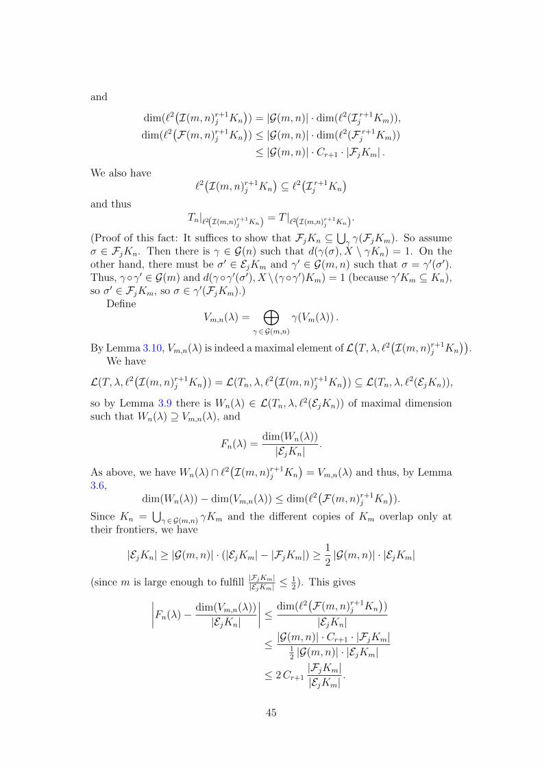
and
dim(`2(I(m,n)r+1
j Kn
)) = |G(m,n)| · dim(`2(I r+1
j Km)),
dim(`2(F(m,n)r+1
j Kn
)) ≤ |G(m,n)| · dim(`2(F r+1
j Km))
≤ |G(m,n)| · Cr+1 · |FjKm| .
We also have`2(I(m,n)r+1
j Kn
)⊆ `2
(I r+1j Kn
)and thus
Tn|`2(I(m,n)r+1j Kn) = T |`2(I(m,n)r+1
j Kn).
(Proof of this fact: It suffices to show that FjKn ⊆⋃γ γ(FjKm). So assume
σ ∈ FjKn. Then there is γ ∈ G(n) such that d(γ(σ), X \ γKn) = 1. On theother hand, there must be σ′ ∈ EjKm and γ′ ∈ G(m,n) such that σ = γ′(σ′).Thus, γγ′ ∈ G(m) and d(γγ′(σ′), X \(γγ′)Km) = 1 (because γ′Km ⊆ Kn),so σ′ ∈ FjKm, so σ ∈ γ′(FjKm).)
DefineVm,n(λ) =
⊕γ ∈G(m,n)
γ(Vm(λ)) .
By Lemma 3.10, Vm,n(λ) is indeed a maximal element of L(T, λ, `2
(I(m,n)r+1
j Kn
)).
We have
L(T, λ, `2(I(m,n)r+1
j Kn
)) = L(Tn, λ, `
2(I(m,n)r+1
j Kn
)) ⊆ L(Tn, λ, `
2(EjKn)),
so by Lemma 3.9 there is Wn(λ) ∈ L(Tn, λ, `2(EjKn)) of maximal dimension
such that Wn(λ) ⊇ Vm,n(λ), and
Fn(λ) =dim(Wn(λ))
|EjKn|.
As above, we have Wn(λ) ∩ `2(I(m,n)r+1
j Kn
)= Vm,n(λ) and thus, by Lemma
3.6,dim(Wn(λ))− dim(Vm,n(λ)) ≤ dim(`2
(F(m,n)r+1
j Kn
)).
Since Kn =⋃γ ∈G(m,n) γKm and the different copies of Km overlap only at
their frontiers, we have
|EjKn| ≥ |G(m,n)| · (|EjKm| − |FjKm|) ≥1
2|G(m,n)| · |EjKm|
(since m is large enough to fulfill|FjKm||EjKm| ≤
12). This gives∣∣∣∣Fn(λ)− dim(Vm,n(λ))
|EjKn|
∣∣∣∣ ≤ dim(`2(F(m,n)r+1
j Kn
))
|EjKn|
≤ |G(m,n)| · Cr+1 · |FjKm|12|G(m,n)| · |EjKm|
≤ 2Cr+1|FjKm||EjKm|
.
45
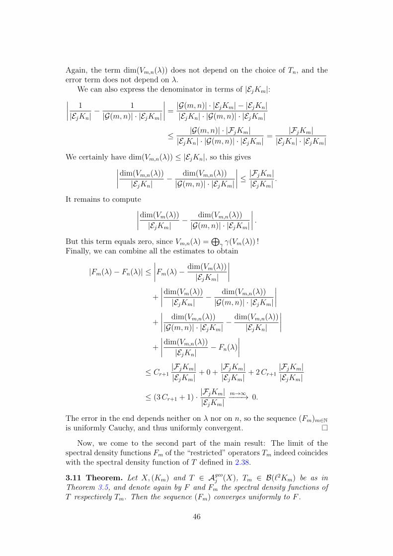
Again, the term dim(Vm,n(λ)) does not depend on the choice of Tn, and theerror term does not depend on λ.
We can also express the denominator in terms of |EjKm|:∣∣∣∣ 1
|EjKn|− 1
|G(m,n)| · |EjKm|
∣∣∣∣ =|G(m,n)| · |EjKm| − |EjKn||EjKn| · |G(m,n)| · |EjKm|
≤ |G(m,n)| · |FjKm||EjKn| · |G(m,n)| · |EjKm|
=|FjKm|
|EjKn| · |EjKm|
We certainly have dim(Vm,n(λ)) ≤ |EjKn|, so this gives∣∣∣∣dim(Vm,n(λ))
|EjKn|− dim(Vm,n(λ))
|G(m,n)| · |EjKm|
∣∣∣∣ ≤ |FjKm||EjKm|
.
It remains to compute∣∣∣∣dim(Vm(λ))
|EjKm|− dim(Vm,n(λ))
|G(m,n)| · |EjKm|
∣∣∣∣ .But this term equals zero, since Vm,n(λ) =
⊕γ γ(Vm(λ)) !
Finally, we can combine all the estimates to obtain
|Fm(λ)− Fn(λ)| ≤∣∣∣∣Fm(λ)− dim(Vm(λ))
|EjKm|
∣∣∣∣+
∣∣∣∣dim(Vm(λ))
|EjKm|− dim(Vm,n(λ))
|G(m,n)| · |EjKm|
∣∣∣∣+
∣∣∣∣ dim(Vm,n(λ))
|G(m,n)| · |EjKm|− dim(Vm,n(λ))
|EjKn|
∣∣∣∣+
∣∣∣∣dim(Vm,n(λ))
|EjKn|− Fn(λ)
∣∣∣∣≤ Cr+1
|FjKm||EjKm|
+ 0 +|FjKm||EjKm|
+ 2Cr+1|FjKm||EjKm|
≤ (3Cr+1 + 1) · |FjKm||EjKm|
m→∞−−−→ 0.
The error in the end depends neither on λ nor on n, so the sequence (Fm)m∈Nis uniformly Cauchy, and thus uniformly convergent.
Now, we come to the second part of the main result: The limit of thespectral density functions Fm of the “restricted” operators Tm indeed coincideswith the spectral density function of T defined in 2.38.
3.11 Theorem. Let X, (Km) and T ∈ Ageoj (X), Tm ∈ B(`2Km) be as in
Theorem 3.5, and denote again by F and Fm the spectral density functions ofT respectively Tm. Then the sequence (Fm) converges uniformly to F .
46
3.12 Definition. To simplify notation, write
trm(T ) :=1
|EjKm|∑
σ∈EjKm
〈σ, Tσ〉 .
as long as the exhaustion (Km) is fixed. This makes sense both for “global”operators T ∈ B(`2X) and for “local” operators Tm ∈ B(`2Km).
3.13 Lemma. Let f : R→ R be continuous and T, Tm as in 3.5. Then
trN f(T ) = limm→∞
trm (f(Tm)) .
(Here, f(T ) is intended as functional calculus in Aj(X), and f(Tm) as func-tional calculus in B(`2(EjKm)).)
Proof. As f is continuous, we have indeed f(T ) ∈ Aj(X), so the trace canbe computed by trN f(T ) = limm→∞ trm
(f(T )
). If f is a polynomial, then
f(Tm)σ = f(T )σ for every σ ∈ Inrj Km, where r is the propagation of T and nis the degree of f . As the nr-neighborhood of the frontier is negligible for thetrace, the claim follows.
For general f , note that (by assumption) the norms ‖Tm‖op |m ∈ N arebounded, and T and all Tm are positive. Thus, there is D > 0 such that[0, D] contains all spectra of T and Tm, and by the Weierstrass approximationtheorem there is a polynomial p with |f(λ)− p(λ)| < ε for all λ ∈ [0, D].
Then, using that both trN and trm have norm one, we obtain∣∣∣trN f(T )− limm→∞
trm (f(Tm))∣∣∣ ≤ |trN f(T )− trN p(T )|
+∣∣∣trN p(T )− lim
m→∞trm (p(Tm))
∣∣∣+∣∣∣ limm→∞
trm (p(Tm))− limm→∞
trm (f(Tm))∣∣∣
≤ ε+ 0 + ε.
As ε was arbitrary, the claim follows.
3.14 Lemma. For all δ > 0 and λ ∈ R define the continuous function
fλ,δ(x) =
1, x ∈ (−∞, λ],
1− x−λδ, x ∈ [λ, λ+ δ],
0, x ∈ [λ+ δ,∞).
Then for every ε > 0 there is δ > 0 (independent of m) such that
|F (λ)− trN fλ,δ(T )| < ε and |Fm(λ)− trm fλ,δ(Tm)| < ε
for all m ∈ N.
47
Proof. First, note that
trN fλ,δ(T ) =
∫Rfλ,δ(x) dF (x),
trm fλ,δ(Tm) =
∫Rfλ,δ(x) dFm(x).
Note that it suffices to let the integrals run over[0, ‖T‖op
].
From now on, focus on the first integral, the second one actually works thesame.
The Lebesgue–Stieltjes integral fulfills the following version of integrationby parts (due to Hewitt, [Hew60]): If in each point either f or g is continuous,then ∫ b
a
f dg +
∫ b
a
g df = f(b+)g(b+)− f(a−)g(a−),
where f(b+) = limx→ b+ f(x), etc. In our case, fλ,δ is everywhere continuous,so the condition is fulfilled. With a = 0 and b = ‖T‖op we have
fλ,δ(b+)F (b+)− fλ,δ(a−)F (a−) = 0 · 1− 1 · 0 = 0.
Thus,
trN fλ,δ(T ) =
∫ b
0
fλ,δ(x) dF (x) = −∫ b
0
F (x) dfλ,δ(x)
= −∫ b
0
F (x)dfλ,δdx
dx =1
δ
∫ λ+δ
λ
F (x) dx.
(Note: While fλ,δ is only almost everywhere differentiable, it is everywherecontinuous, and thus, no single point has positive measure in dfλ,δ, and we canleave out the two non-differentiable points λ and λ + δ. On the rest of theinterval, df = df
dxdx holds.) The same argument applied to Fm yields
trm fλ,δ(Tm) =1
δ
∫ λ+δ
λ
Fm(x) dx.
Every spectral density function is right-continuous and non-decreasing.Thus, there is δ∞ > 0 such that |F (λ)− F (x)| < ε for all x ∈ [λ, λ+ δ∞].
By Theorem 3.5, the functions Fm are uniformly convergent to some func-tion Flim, so there is M such that |Fm(x)− Flim(x)| < ε/3 for all m ≥M . As alimit of right-continuous functions, Flim is right-continuous. Thus, there is δlim
such that |Flim(λ)− Flim(x)| < ε/3 for all x ∈ [λ, λ+ δlim], and that implies
|Fm(λ)− Fm(x)|< |Fm(λ)− Flim(λ)|+ |Flim(λ)− Flim(x)|+ |Flim(x)− Fm(x)| < ε
for all m ≥M and all x ∈ [λ, λ+ δlim].
48
Finally, for each of the functions F1, F2, . . . , FM−1, there is a δm > 0 suchthat |Fm(λ)− Fm(x)| < ε for all x ∈ [λ, λ+ δm].
Setting δ = min(δ1, . . . , δM−1, δlim, δ∞), we get indeed
|F (λ)− trN fλ,δ(T )| < ε and |Fm(λ)− trm fλ,δ(Tm)| < ε
for all m ∈ N and all x ∈ [λ, λ+ δ].
Proof of Theorem 3.11. First show pointwise convergence.Fix ε > 0. By Lemma 3.14, there are δ > 0 and a continuous function fλ,δ
such that
|F (λ)− trN fλ,δ(T )| < ε
3and |Fm(λ)− trm fλ,δ(Tm)| < ε
3
for all m ∈ N.By Lemma 3.13, the function fλ,δ satisfies
trN fλ,δ(T ) = limm→∞
trm (fλ,δ(Tm)) ,
so there is M ∈ N such that for every m ≥M ,
|trN fλ,δ(T )− trm (fλ,δ(Tm))| < ε
3.
Thus, for every m ≥M ,|F (λ)− Fm(λ)| < ε.
This proves pointwise convergence, and thus, F (λ) = Flim(λ) for all λ ∈ R. Aswe already know that Fm → Flim uniformly, uniform convergence follows.
3.3 Different normalizations
From an algebraical point of view, it is natural to normalize the trace onB(`2(EjKm)
)by the dimension of that space, that is, by |EjKm|. (This turns
the normalized trace into a state, that is, a linear functional of norm one. Inparticular, it leads to dimN (Hj) = trN (id) = 1.) Topologically, however, thisis not the most useful normalization:
First, it causes problems when we want to compare L2-invariants of differentdimensions, e. g. when computing Euler characteristics. For this, it is desirableto divide all traces on B
(`2(EjKm)
)(for the various values of j) by the same
number.Second, it is unsuitable for comparing different self-similar CW-complexes.
For example, different CW-structures on the same complex will often result indifferent numbers of cells (in any dimension), but they should not change thetopological invariants.
Third, it proves to be unfortunate for product spaces, where we need thenormalizations on X, Y and X × Y to be compatible, but |EjKm| · |EjLm| 6=|Ej(Km × Lm)| for any j ≥ 1.
49
There are several possibilities for this normalization factor – one mightchoose the number of vertices, or of top-dimensional cells, or even the numberof local isomorphisms in G(1,m) (that is, how many copies of K1 are needed to“build” Km). To show that all of these normalizations are indeed equivalent(in so far as they only produce a constant prefactor to the trace), let us showthat their ratios converge:
3.15 Lemma. (a) For every j ∈ N0, the limit limm→∞
|EjKm||G(1,m)|
exists.
(b) If EjX 6= ∅, then limm→∞
|EjKm||G(1,m)|
> 0.
Proof. (a) We have Km+1 =⋃γ ∈G(m,m+1) γKm and therefore |EjKm+1| ≤
|G(m,m+ 1)| · |EjKm|, while |G(1,m+ 1)| = |G(1,m)| · |G(m,m+ 1)|. Thus,
|EjKm+1||G(1,m+ 1)|
≤ |G(m,m+ 1)| · |EjKm||G(1,m)| · |G(m,m+ 1)|
≤ |EjKm||G(1,m)|
for all m. Hence, the sequence( |EjKm||G(1,m)|
)m
is non-increasing (and bounded from
below by 0), so it converges.(b) If X contains any j-cell, then amenability demands that there is m0 ∈ N
such that |EjKm| > |FjKm| for all m ≥ m0. Then, we have for all m ≥ m0
and thus also for the limit m→∞,
|EjKm||G(1,m)|
≥ |G(m0,m)| · (|EjKm0| − |FjKm0|)|G(1,m0)| · |G(m0,m)|
≥ 1
|G(1,m0)|> 0.
3.16 Remark. We can define the shorthand
|EjX||G(1,∞)|
= limm→∞
|EjKm||G(1,m)|
.
Note, however, that this depends on the choice of (Km): For example, if asecond exhaustion were given by Lm = Km+1 with the local isomorphismsG ′(m,n) = G(m+ 1, n+ 1), then we would obtain
limm→∞
|EjLm||G ′(1,m)|
= limm→∞
|EjKm+1||G(2,m+ 1)|
= |G(1, 2)| · limm→∞
|EjKm||G(1,m)|
.
In contrast, the ratio of cell numbers is an intrinsic property of X itself:
3.17 Definition and Lemma. For any j, k ∈ N0 such that EkX 6= ∅, thelimit
|EjX||EkX|
:= limm→∞
|EjKm||EkKm|
exists and is independent of the exhaustion (Km). If EjX 6= ∅, the limit ispositive.
50
Proof. The existence follows directly from Lemma 3.15; it remains to show theindependence of (Km). A general proof is given in [Suc16] (Lemma 4.12); asan illustration, let us give the (much shorter) proof for the simplicial case here:
Consider specifically k = 0 and define T ∈ Ageo0 (X) as
Tρ =|σ ∈ EjX | ρ ∈ σ|
j + 1ρ.
As every j-simplex contains exactly j + 1 vertices, this immediately yields
trm T =1
|E0Km|∑
ρ∈E0Km
1
j + 1
∑σ∈EjKmρ∈σ
1 =1
|E0Km|∑
σ∈EjKm
1
j + 1
∑ρ∈E0Kmρ∈σ
1
=1
|E0Km|∑
σ∈EjKm
1 =|EjKm||E0Km|
.
Now the claim follows from Theorem 3.4, as trA(T ) = limm→∞ trKm(T ) isindependent of the choice of (Km). Finally, for k > 0, simply use
limm→∞
|EjKm||EkKm|
=limm→∞
|EjKm||E0Km|
limm→∞
|EkKm||E0Km|
.
For the positivity of the limit, combine this result with Lemma 3.15 (b).
51
4 L2-Betti numbers and Novikov–Shubin in-
variants
Let us now turn towards the actual L2-invariants that can be derived from thespectral density functions of Laplacians. First among these are the L2-Bettinumbers, which simply measure the sizes of the kernels of the Laplacians, orthe amount of “harmonic chains” on the complex. Second, we will considerNovikov–Shubin invariants, which look at the spectrum near (but not at) zero;one might say that they measure the amount of “almost harmonic chains” onthe complex.7
For both of these invariants, we will look at two main questions:
(a) We will justify the name “invariants” by proving that they are indeedinvariant under suitable homotopies. This, of course, requires to first con-struct the notion of a self-similar homotopy compatible with the structureof the spaces.
(b) We will attempt to approximate the invariants by their equivalents onfinite subcomplexes. For L2-Betti numbers, this turns out to be a sim-ple corollary; for Novikov–Shubin invariants the situation is much morecomplicated.
4.1 Approximation of L2-Betti numbers
The L2-Betti numbers of an operator measure the size of its kernel – although,strictly speaking, the “kerT” in the following definition is a subspace of Hj,not of `2(EjX), so we do not directly measure how many chains in `2(EjX) getmapped to zero!
Nonetheless, L2-Betti numbers measure a “failure to be injective”, and theapproximation result below shows that their values are very much correlatedwith the behavior of the operator on `2(EjX).
4.1 Definition. Given a positive operator T ∈ Nj, the L2-Betti number of Tis
b(2)(T ) = F T (0) = dimN (kerT ).
Given a self-similar complex X, define its j-th L2-Betti number as
b(2)j (X) = b(2)
(∆
(X)j
).
In this chapter, dimN is normalized such that the total space has dimensionone. As mentioned in 3.3, it is occasionally useful to use other normalizations;we will use a different one in Chapter 6.
7The third main invariant (L2-torsion and the Fuglede–Kadison determinants necessaryto construct it) will be considered in the next chapter.
52
As L2-Betti numbers are simply the values of the spectral density functionsat zero, their approximation follows directly from the work done in the previouschapter:
4.2 Corollary. Let X be a self-similar CW-complex with self-similar exhaus-tion (Km)m∈N. Denote by
βj(Km) = dimCHj(Km;C)
the classical Betti numbers of Km, and by
b(2)j (X) = dimN
(ker ∆
(X)j
)the L2-Betti numbers of X. Then
b(2)j (X) = lim
m→∞
βj(Km)
|EjKm|.
Proof. In Theorem 3.11, put T = ∆(X)j and Tm = ∆
(Km)j . Then b
(2)j (X) = F (0)
andβj(Km)
|EjKm| = Fm(0), and convergence follows.
In the classical case, L2-Betti numbers over (elementary) amenable groupscan often only take certain rational values.8 For our version of self-similarcomplexes, we cannot expect such a restriction:
4.3 Example. Given any number y ∈ [0, 1], write y =∑∞
j=1 yj2−j with yj ∈
0, 1, and define complexes (Km)∞m=0 as follows:Let K0 = [0, 1]2 be a square with the standard CW-structure. If ym = 0,
define Km as the union of two copies of Km−1 that are glued together alongan edge. If ym = 1, instead define Km as the union of two copies of Km−1 thatare glued together only at the two endpoints of an edge. (See Figure 8.)
With β1(K0) = 0 and |E1K0| = 4, we obtain
β1(Km) = 2 · β1(Km−1) + ym =m∑j=1
2m−jyj,
|E1Km| = 2 · |E0Km−1|+ ym − 1 = 2m · 4 +m∑j=1
2m−j(yj − 1)
= 3 · 2m − 1 +m∑j=1
2m−jyj.
Thus, if we set X =⋃∞m=0Km,
b(2)1 (X) = lim
m→∞
β1(Km)
|E1Km|=
y
y + 3,
and therefore any number between 0 and 1/4 appears as the first L2-Bettinumber of such a complex.
8This is a special case of Atiyah’s conjecture, compare [DLM+03].
53
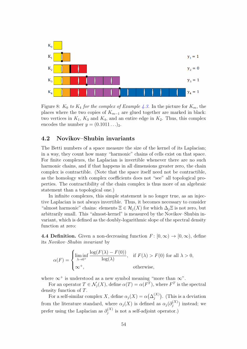
Figure 8: K0 to K4 for the complex of Example 4.3. In the picture for Km, theplaces where the two copies of Km−1 are glued together are marked in black:two vertices in K1, K3 and K4, and an entire edge in K2. Thus, this complexencodes the number y = (0.1011 . . .)2.
4.2 Novikov–Shubin invariants
The Betti numbers of a space measure the size of the kernel of its Laplacian;in a way, they count how many “harmonic” chains of cells exist on that space.For finite complexes, the Laplacian is invertible whenever there are no suchharmonic chains, and if that happens in all dimensions greater zero, the chaincomplex is contractible. (Note that the space itself need not be contractible,as the homology with complex coefficients does not “see” all topological pro-perties. The contractibility of the chain complex is thus more of an algebraicstatement than a topological one.)
In infinite complexes, this simple statement is no longer true, as an injec-tive Laplacian is not always invertible. Thus, it becomes necessary to consider“almost harmonic” chains: elements Ξ ∈ Hj(X) for which ∆jΞ is not zero, butarbitrarily small. This “almost-kernel” is measured by the Novikov–Shubin in-variant, which is defined as the doubly-logarithmic slope of the spectral densityfunction at zero:
4.4 Definition. Given a non-decreasing function F : [0,∞) → [0,∞), defineits Novikov–Shubin invariant by
α(F ) =
lim infλ→0+
log(F (λ)− F (0))
log(λ), if F (λ) > F (0) for all λ > 0,
∞+, otherwise,
where ∞+ is understood as a new symbol meaning “more than ∞”.For an operator T ∈ Nj(X), define α(T ) = α(F T ), where F T is the spectral
density function of T .For a self-similar complex X, define αj(X) = α
(∆
(X)j
). (This is a deviation
from the literature standard, where αj(X) is defined as αj(∂(X)j ) instead; we
prefer using the Laplacian as ∂(X)j is not a self-adjoint operator.)
54
Novikov–Shubin invariants can take any value in [0,∞] as well as the addi-tional value∞+, which indicates a spectral gap around zero: α(F ) is set to∞+
whenever F is constant on an interval [0, ε) for some ε > 0; if F is the spectraldensity function of some operator T , this implies that spec(T ) ∩ (0, ε) = ∅. IfT is injective, this implies that it is bounded from below by ε, and conversely,every operator that is bounded from below will exhibit this spectral gap. Asbeing bounded from below is equivalent to invertibility, this shows:
4.5 Lemma. An operator T ∈ Nj(X) is invertible if and only if ker(T ) = 0and α(T ) =∞+.
4.6 Remark. A space X is said to have the limit property if the limit inferiorin 4.4 is a true limit. Luck notes that every G-CW-complex known to him hasthe limit property ([Luc02], page 92, Remark 2.42).
It is not hard to write down a function that does not fulfill the limit prop-erty; for example, let
F (0) = 0 and F (λ) = 2−k if λ ∈ [2−2k, 2−k) for k ∈ N.
Then clearly
α(F ) = lim infλ→0+
log(F (λ)− F (0))
log(λ)=
1
2but lim sup
λ→0+
log(F (λ)− F (0))
log(λ)= 1.
However, it is unclear whether such a counterexample could occur as the spec-tral density function of a Laplacian of a self-similar complex.
Let us quickly note some obvious properties of Novikov–Shubin invariants offunctions. Most of these follow trivially from the definition; compare [Luc02],p. 77 ff.
4.7 Lemma. Let F,G : [0,∞) → [0,∞) be non-decreasing and r > 0. Then(using r · ∞ =∞ and r · ∞+ =∞+)
α(r · F (λ)) = α(F (λ)),
α(F (r · λ)) = α(F (λ)),
α(F (λr)) = r · α(F (λ)),
α(F +G) = min(α(F ), α(G)
),
and, if F (0) = G(0), then
F ≤ G =⇒ α(F ) ≥ α(G).
4.8 Definition and Lemma. Two non-decreasing functions F,G : [0,∞)→[0,∞) are dilatationally equivalent , written F ' G, if there are ε, C > 0 suchthat
F (λ) ≤ G(Cλ) and G(λ) ≤ F (Cλ) for all λ ∈ [0, ε).
In that case,α(F ) = α(G).
55
Proof. This is a direct consequence of Lemma 4.7.
4.9 Corollary. Let X be a self-similar complex. For any two operators S, T ∈Nj(X) we have the following properties:
(a) α(T ∗T ) = α(TT ∗) = 12α(T ∗) = 1
2α(T ).
(b) If S is invertible, then α(ST ) = α(TS) = α(T ).
Proof. (a) This follows from Lemmas 2.40 and 4.7.
(b) If S is invertible, there is a constant C > 0 such that C−1 ‖Ξ‖ ≤ ‖SΞ‖ ≤C ‖Ξ‖ for all Ξ ∈ Hj. Therefore, if V ⊆ Hj is a subspace fulfilling‖T |V ‖ ≤ λ, then ‖ST |V ‖ ≤ Cλ, so Lemma 2.42 yields F (ST )(Cλ) ≥F (T )(λ).
Conversely, if W ⊆ Hj is a subspace fulfilling ‖ST |W‖ ≤ C−1λ, then‖T |V ‖ ≤ λ, so Lemma 2.42 yields F (T )(λ) ≥ F (ST )(C−1λ).
Now α(ST ) = α(T ) follows from Lemma 4.8, and since S∗ is also invert-ible, part (a) gives α(TS) = α((TS)∗) = α(S∗T ∗) = α(T ∗) = α(T ).
Even though we mostly work with the Laplacians ∆j, we will sometimesneed to refer back to the boundary operators ∂j. To this end, we use thefollowing relation:
4.10 Corollary. Let X be a self-similar complex, and ∂j : `2(EjX)→ `2(Ej−1X)the differential in its L2-chain complex. Then
αj(∆j) = min
(α(∂j)
2,α(∂j+1)
2
).
Proof. Define ∆j− = ∂∗j ∂j and ∆j+ = ∂j+1∂∗j+1, so the Laplacian takes the
form ∆j = ∆j− + ∆j+. (Of course, both of the operators ∆j± are geomet-ric.) By definition, F (∂j)(λ) = F (∆j−)(λ2), and by Lemma 2.40 we also haveF (∂j+1)(λ) = F (∂∗j+1)(λ) = F (∆j+)(λ2). Therefore, Lemma 4.7 gives
α(∆j−) =α(∂j)
2and α(∆j+) =
α(∂j+1)
2.
It is a well-known fact that on every finite CW-complex, the chain complexcan be decomposed into the orthogonal sum
C[EjX] = ker(∆j)⊕ im(∂∗j )⊕ im(∂j+1),
and that w. r. t. this decomposition, the Laplacian takes the form
∆j =
0 0 00 ∆j− 00 0 ∆j+
.
56
Therefore, the (renormalized) spectral density function on every finite subcom-plex Km ⊆ X fulfills
F(∆
(Km)j
)= F
(∆
(Km)j−
)+ F
(∆
(Km)j+
).
By Theorem 3.11, the same holds on X:
F(∆
(X)j
)= F
(∆
(X)j−)
+ F(∆
(X)j+
).
Now the claim follows from Lemma 4.7.
4.3 Homotopy invariance of L2-Betti numbers
The name L2-invariant refers to homotopy invariance. However, this can-not mean invariance under any homotopy: For example, all of the complexesdefined in Example 4.3 (except for the one corresponding to y = 0) are ho-motopy equivalent, yet their L2-Betti numbers take many different values.Namely, each of these complexes has countably many holes, but their densityis different – something that a conventional homotopy cannot account for.
Thus, a homotopy of self-similar complexes must in some way preservethe self-similar structure to have any chance of preserving our version of L2-invariants. It is important to note that the self-similar structure on a complexis not part of the space itself – rather, a complex is self-similar as soon as thereis at least one such structure, and the invariants are independent of its choice.Therefore, it should suffice that a self-similar map is compatible with someself-similar structure on each space:
4.11 Definition. Let X and Y be self-similar complexes. A map f : X → Yis a self-similar map if there are self-similar structures
(Km,G(m,m + 1)
)on
X and(Lm,G ′(m,m+ 1)
)on Y such that for all m:
(a) f(Km) ⊆ Lm,
(b) there is a bijection ϕm : G(m,m+ 1)→ G ′(m,m+ 1),
(c) and the map is “equivariant” with respect to these local isomorphisms;that is, the following diagram commutes for each γ ∈ G(m,m+ 1):
Kmγ //
f
γKm
f
Lmϕm(γ) // ϕm(γ)Lm
A homotopy equivalence requires four such maps (one in each directionand a homotopy in each space), and it appears necessary that all of them usethe same structure:
57
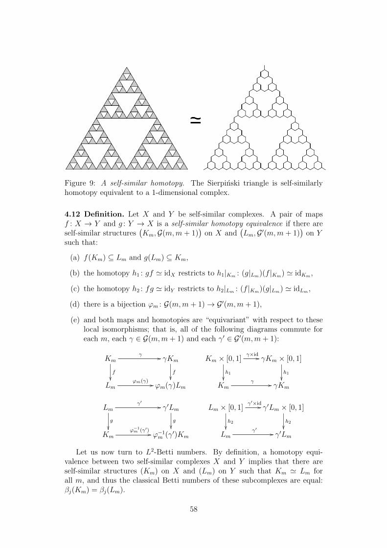
Figure 9: A self-similar homotopy. The Sierpinski triangle is self-similarlyhomotopy equivalent to a 1-dimensional complex.
4.12 Definition. Let X and Y be self-similar complexes. A pair of mapsf : X → Y and g : Y → X is a self-similar homotopy equivalence if there areself-similar structures
(Km,G(m,m + 1)
)on X and
(Lm,G ′(m,m + 1)
)on Y
such that:
(a) f(Km) ⊆ Lm and g(Lm) ⊆ Km,
(b) the homotopy h1 : gf ' idX restricts to h1|Km : (g|Lm)(f |Km) ' idKm ,
(c) the homotopy h2 : fg ' idY restricts to h2|Lm : (f |Km)(g|Lm) ' idLm ,
(d) there is a bijection ϕm : G(m,m+ 1)→ G ′(m,m+ 1),
(e) and both maps and homotopies are “equivariant” with respect to theselocal isomorphisms; that is, all of the following diagrams commute foreach m, each γ ∈ G(m,m+ 1) and each γ′ ∈ G ′(m,m+ 1):
Kmγ //
f
γKm
f
Lmϕm(γ) // ϕm(γ)Lm
Km × [0, 1]γ×id //
h1
γKm × [0, 1]
h1
Kmγ // γKm
Lm
g
γ′ // γ′Lm
g
Km
ϕ−1m (γ′) // ϕ−1
m (γ′)Km
Lm × [0, 1]γ′×id//
h2
γ′Lm × [0, 1]
h2
Lmγ′ // γ′Lm
Let us now turn to L2-Betti numbers. By definition, a homotopy equi-valence between two self-similar complexes X and Y implies that there areself-similar structures (Km) on X and (Lm) on Y such that Km ' Lm forall m, and thus the classical Betti numbers of these subcomplexes are equal:βj(Km) = βj(Lm).
58
By Corollary 4.2, the L2-Betti numbers of X and Y can be approximatedby βj(Km) and βj(Lm), but only after normalization – and our usual normali-zation factor is the number of cells (of some dimension) in each subcomplex,which is certainly not homotopy invariant.
By Lemma 3.15, the limits limm→∞
|EjKm||G(1,m)| and lim
m→∞|EjLm||G′(1,m)| exist, and by
property 4.12 (d) we have |G(1,m)| = |G ′(1,m)|. Thus, the limit limm→∞
|EjKm||EjLm|
exists as well, and we can write
b(2)j (X) = lim
m→∞
βj(Km)
|EjKm|= lim
m→∞
βj(Lm)
|EjKm|= lim
m→∞
|EjLm||EjKm|
· limm→∞
βj(Lm)
|EjLm|
= limm→∞
|EjLm||EjKm|
· b(2)j (Y ).
This already proves that if b(2)j (X) = 0, then also b
(2)j (Y ) = 0.
If the j-th Betti numbers are non-zero, it remains to show that the normal-ization factor lim
m→∞|EjLm||EjKm| does not depend on the choices of (Km) and (Lm):
Assume (K ′m) and (L′m) are other self-similar exhaustions of X and Y suchthat K ′m ' L′m for every m. Again, we obtain βj(K
′m) = βj(L
′m). From
Corollary 4.2 we see that
limm→∞
βj(Km)
|EjKm|= b
(2)j (X) = lim
m→∞
|βj(K ′m)||EjK ′m|
,
limm→∞
βj(Lm)
|EjLm|= b
(2)j (Y ) = lim
m→∞
|βj(L′m)||EjL′m|
.
Therefore, using Km ' Lm and K ′m ' L′m,
limm→∞
|EjK ′m||EjKm|
= limm→∞
βj(K′m)
β(Km)= lim
m→∞
βj(L′m)
β(Lm)= lim
m→∞
|EjL′m||EjLm|
,
and thus indeed
limm→∞
|EjK ′m||EjL′m|
= limm→∞
|EjKm||EjLm|
.
This yields the following statement:
4.13 Theorem. If two self-similar complexes X and Y are homotopy equiv-alent in the sense of Definition 4.12, then their L2-Betti numbers are relatedby the formula
b(2)j (X) = lim
m→∞
|EjLm||EjKm|
· b(2)j (Y )
where the factor limm→∞
|EjLm||EjKm| is the same for any two self-similar exhaustions
(Km), (Lm) that fulfill Km ' Lm for every m.
59
4.4 Homotopy invariance of Novikov–Shubin invariants
Unlike L2-Betti numbers, Novikov–Shubin invariants are not affected by nor-malization factors: Since they only use the logarithm of the spectral densityfunction, any constant factor becomes negligible. That allows us to obtain“true” invariance under self-similar homotopy equivalences:
4.14 Theorem. If two self-similar complexes X and Y are homotopy equiv-alent in the sense of Definition 4.12, then their Novikov–Shubin invariantsare equal. More precisely, we have both α
(∂
(X)j
)= α
(∂
(Y )j
)and α
(∆
(X)j
)=
α(∆
(Y )j
)for all j.
In order to work with self-similar maps, we first need to prove that theyindeed induce bounded operators on the L2-chain complex:
4.15 Lemma. Let f : X → Y be a self-similar map. Then the induced chainmaps fj : C[EjX]→ C[EjY ] are bounded, and thus extend to bounded operatorsfj : `2(EjX)→ `2(EjY ).
Proof. Use the same notation as before: (Km) is a self-similar exhaustion of Xwith local isomorphisms G(m,m+1), and (Lm) is the corresponding self-similarexhaustion of Y with local isomorphisms G ′(m,m+ 1)
Choose m large enough that Lm has a non-frontier cell. Then there is aconstant D such that every γLm (for γ ∈ G ′(m)) overlaps at most D other suchcopies of Lm. Namely, let r be the maximal combinatorial distance betweenvertices in Lm (this is finite, as we assume Lm to be connected). Then, for anyvertex ρ ∈ E0(γLm), the 2r-ball around ρ contains an interior vertex of everyother copy γ′Lm that intersects γLm. As different translates only overlap attheir frontiers, all these interior vertices are distinct, and as the complex Y isbounded, B2r(ρ) is finite. Thus, we can set D = |B2r(ρ)|.
Write x ∈ C[EjX] as a sum∑
γ∈G(m) xγ, where the xγ ∈ C[Ej(γKm)] aremutually orthogonal and only finitely many xγ are nonzero. By assumption,fj(xγ) ∈ C[ϕ(γ)Lm] for some ϕ(γ) ∈ G ′(m), but since the translates of Lm canoverlap at their frontiers, the fj(xγ) are not necessarily mutually orthogonal.
Enumerate the γ ∈ G(m) with xγ 6= 0 as γ1, . . . , γN such that
‖fj(xγ1)‖ ≥ ‖fj(xγ2)‖ ≥ . . . ≥ ‖fj(xγN )‖ .
Then, in the sum
‖fj(x)‖2 =N∑
i,k=1
〈fj(xγi), fj(xγk)〉
there are at most 2D nonzero terms containing f(xγ1), because supp(f(xγ1)) ⊆ϕ(γ1)(Lm) and ϕ(γ1)Lm intersects at most D other translates ϕ(γk)Lm. Eachof those terms fulfills∣∣〈fj(xγ1), fj(xγk)〉∣∣ ≤ ‖fj(xγ1)‖ · ‖fj(xγk)‖ ≤ ‖fj(xγ1)‖2 .
60
Thus,
‖fj(x)‖2 ≤ 2D ‖fj(xγ1)‖2 +
N∑i,k=2
〈fj(xγi), fj(xγk)〉 ,
and by induction we obtain
‖fj(x)‖2 ≤ 2DN∑i=1
‖fj(xγi)‖2 .
Finally, since f commutes with local isomorphisms, so does fj, and thus
‖fj(xγi)‖ ≤∥∥fj|C[EjKm]
∥∥ · ‖xγ‖for all γ. We conclude
‖fj‖ ≤√
2D∥∥fj|C[EjKm]
∥∥ ,and
∥∥fj|C[EjKm]
∥∥ is finite because EjKm is finite.
4.16 Remark. Given a self-similar homotopy h : X × [0, 1] → Y between twomaps X → Y , the induced chain homotopy ηj : C[EjX] → C[Ej+1Y ] can beobtained as (−1)j times the restriction of
hj : C[Ej+1
(X × [0, 1]
)]→ C[Ej+1Y ],
using the Kunneth isomorphism
Ej+1
(X × [0, 1]
) ∼= Ej+1X t Ej+1X t EjX.
(Compare [Luc05], page 61.) Applying Lemma 4.15 to hj therefore also provesthat ηj is bounded.
As a preparation for the proof of homotopy invariance, let us show thatif two finite CW-complexes are homotopy equivalent, then the spectral den-sity functions of their differentials are dilatationally equivalent in a preciselycontrolled way:
4.17 Lemma. Let Kf // Lgoo be a homotopy equivalence between two finite
CW-complexes with homotopies h1 : gf ' idK and h2 : fg ' idL, and letη1,j : C[EjK] → C[Ej+1K] and η2,j : C[EjL] → C[Ej+1L] be the chain homo-topies induced by h1 and h2.
Denote by Fnn(∂j) the non-normalized spectral density functions of the dif-ferentials, and let F⊥nn(∂j)(λ) = Fnn(∂j)(λ)− Fnn(∂j)(0). Then
Fnn(∂Kj )⊥(λ) ≤ Fnn(∂Lj )⊥(2 ‖fj−1‖ ‖gj‖λ)
Fnn(∂Lj )⊥(λ) ≤ Fnn(∂Kj )⊥(2 ‖gj−1‖ ‖fj‖λ)
for all
0 < λ < min
(1
2 ‖η1,j−1‖,
1
2 ‖η2,j−1‖
).
61
Proof. Fix j and λ and let V ⊆ C[EjK] be the vector space spanned by alleigenvectors of (∂Kj )∗∂Kj with eigenvalues ≤ λ2. (In other words, this is theimage of the spectral projection E(λ) for the operator ∂Kj .)
Furthermore, let
Pj : C[EjK]→ ker(∂Kj )⊥, Qj : C[EjL]→ ker(∂Lj )⊥
be the orthogonal projections. Thus, the non-normalized spectral density func-tion of ∂Kj takes the values
Fnn(∂Kj )(λ) = dim(V ),
Fnn(∂Kj )⊥(λ) = Fnn(∂Kj )(λ)− Fnn(∂Kj )(0) = dim(PjV ).
DefineW = QjfjPjV.
Let x ∈ PjV and write fj(x) = y + z with y = Qjfj(x) ∈ W and z ∈ ker(∂Lj ).By definition of the chain homotopy, we have
x = gj(y) + gj(z) + η1,j−1∂Kj (x) + ∂Kj+1η1,j(x).
However, g∗ commutes with the differentials, so ∂Kj gj(z) = gj−1∂Lj (z) = 0.
Thus, both the second and the fourth summand lie in ker(∂Kj ) ⊥ x, and weobtain
x = Pjx = Pjgj(y) + Pjη1,j−1∂Kj (x).
By choice of x and λ, we have
‖x‖ ≤ ‖Pjgj(y)‖+∥∥Pjη1,j−1∂
Kj (x)
∥∥≤ ‖gj(y)‖+ ‖η1,j−1‖
∥∥∂Kj (x)∥∥
≤ ‖gj‖ ‖y‖+ ‖η1,j−1‖λ ‖x‖
≤ ‖gj‖ ‖y‖+1
2‖x‖
=⇒ ‖x‖ ≤ 2 ‖gj‖ ‖y‖ .
This proves that Qjfj : PjV → W,x 7→ y is bounded from below and thereforeinjective, so
dim(PjV ) = dim(W ).
Elements of W are trivially orthogonal to the kernel of ∂Lj , and furthermore,∥∥∂Lj (y)∥∥ =
∥∥∂Lj fj(x)∥∥ =
∥∥fj−1∂Kj (x)
∥∥≤ ‖fj−1‖
∥∥∂Kj x∥∥ ≤ ‖fj−1‖λ ‖x‖≤ 2λ ‖fj−1‖ ‖gj‖ ‖y‖ ,
so the finite-dimensional analogue of Lemma 2.42 shows that
Fnn(∂Lj )⊥(2 ‖fj−1‖ ‖gj‖λ) ≥ dim(W ) = dim(PjV ) = Fnn(∂Kj )⊥(λ).
This proves the first estimate. To prove the second estimate, simply swap Kwith L, f with g, and η1 with η2.
62
Now we can use approximation of spectral density functions to prove 4.14:
Proof of Thm. 4.14. Use all notation from Def. 4.12.The maps f, g and the homotopies h1, h2 induce chain maps and chain
homotopies
fj : C[EjX]→ C[EjY ] gj : C[EjY ]→ C[EjX]
η1,j : C[EjX]→ C[Ej+1X] η2,j : C[EjY ]→ C[Ej+1Y ]
on the cellular (non-L2) chain complexes of X and Y . By assumption, themaps can be restricted to Km and Lm, and thus the same applies to theirinduced maps on the chain complexes, yielding
fj : C[EjKm]→ C[EjLm] gj : C[EjLm]→ C[EjKm]
η1,j : C[EjKm]→ C[Ej+1Km] η2,j : C[EjLm]→ C[Ej+1Lm]
On the other hand, Lemma 4.15 and Remark 4.16 show that all these chainmaps are indeed bounded operators. Thus, they extend to the L2-chain com-plexes `2(EjX) resp. `2(EjY ), and we can estimate
∥∥fj|C[EjKm]
∥∥ ≤ ‖fj‖, andthe same for gj, η1,j and η2,j. Especially, these norms are bounded uniformlyin m.
Apply Lemma 4.17 to Km and Lm to get
Fnn(∂Kmj )⊥(λ) ≤ Fnn(∂Lmj )⊥(√
C · λ)
Fnn(∂Lmj )⊥(λ) ≤ Fnn(∂Kmj )⊥(√
C · λ)
for all λ ∈ (0, ε), where
√C = max
(2 ‖fj−1‖ ‖gj‖ , 2 ‖gj−1‖ ‖fj‖
)ε = min
(1
2 ‖η1,j−1‖,
1
2 ‖η2,j−1‖
)and neither ε nor C depend on m.
Remember that Fnn(∂j)⊥(λ) = Fnn(∆j−)⊥(λ2). Therefore, we have
Fnn(∆Kmj− )⊥(λ) ≤ Fnn(∆Lm
j− )⊥(C · λ
)Fnn(∆Lm
j− )⊥(λ) ≤ Fnn(∆Kmj− )⊥
(C · λ
)and furthermore, ∆X
j− and ∆Yj− are geometric operators, they are approximated
by ∆Kmj− and ∆Lm
j− , and Theorem 3.11 is applicable. However, in order to applyit, we have to renormalize:
Recall from Lemma 3.15 that the limits
limm→∞
|EjKm||G(1,m)|
and limm→∞
|EjLm||G ′(1,m)|
exist and are nonzero whenever EjX 6= ∅ 6= EjY . We are assuming that
|G(1,m)| = |G ′(1,m)|
63
for all m. Thus, the limit
r = limn→∞
|EjLm||EjKm|
exists, and we get from 3.11 that for every λ ∈ (0, ε),
F (∆Xj−)(λ) = lim
m→∞
Fnn(∆Kmj− )(λ)
|EjKm|≤ lim
m→∞
Fnn(∆Lmj− )⊥(Cλ)
|EjKm|
= r · limm→∞
Fnn(∆Lmj− )⊥(Cλ)
|EjLm|= r · F (∆Y
j−)(Cλ)
and, by the same argument,
r · F (∆Yj−)(λ) ≤ F (∆X
j−)(Cλ).
Now, Lemmas 4.7 and 4.8 yield
α(F (∆X
j−))
= α(r · F (∆Y
j−))
= α(F (∆Y
j−))
and thusα(∂
(X)j ) = 2α(∆X
j−) = 2α(∆Yj−) = α(∂
(Y )j ).
Finally, the statement for ∆ follows from Corollary 4.10.
4.5 Novikov–Shubin invariants, random walks andgrowth
Betti numbers have a clear topological meaning (“counting holes in a space”),and their approximation carries that meaning over to L2-Betti numbers (count-ing the “frequency of holes”). It is significantly harder to ascribe such meaningto Novikov–Shubin invariants, especially since they are completely trivial forfinite subspaces. (The spectral density function of any operator on a finitecomplex is always a step function, giving it α =∞+.)
For the classical Novikov–Shubin invariants of (Laplacians on) spaces witha suitable group action, there is indeed a geometrical (though not truly topo-logical) meaning of at least the zeroth Novikov–Shubin number:
4.18 Definition. Let G be a finitely generated infinite group and C its Cayleygraph with regard to some finite generating set S. Let d be the combinatorialdistance of vertices of C (or, equivalently, the word metric of G with respectto S), and
Br(e) = g ∈ G | d(e, g) ≤ r .
G has polynomial growth, if there is a number d > 0 such that
|Br(e)| ∼ rd,
and in that case, d is called the degree of growth of G. (It turns out that ddoes not depend on the choice of S.)
64
All infinite virtually nilpotent groups have polynomial growth ([Gro81]),and the degree of growth is closely linked to the first Novikov–Shubin invariant.This theorem is originally due to Lott ([Lot92]); we cite the fully generalizedversion from Luck ([Luc02], Lemmas 2.45 and 2.46):
4.19 Theorem. Let G be a finitely generated group and X a connected freeG-CW-complex of finite type.
(a) If G is finite or not amenable, α1(X) =∞+.
(b) If G is infinite and amenable, but not virtually nilpotent, α1(X) =∞.
(c) If G is infinite and virtually nilpotent, α1(X) equals the degree of growthof G.
However, the proof of this theorem, as given by Luck, makes it clear thatα and the degree of growth are not directly related to each other. Rather,they are both connected to a third quantity: the return probability of randomwalks.
For any vertex ρ ∈ E0X, let S1(ρ) = σ ∈ E0X | dcomb(ρ, σ) = 1 (this isthe set of all neighboring vertices of ρ), and define the transition operator
P : `2(E0X)→ `2(E0X), ρ 7→ 1
|S1(ρ)|∑
σ∈S1(ρ)
σ.
Then 〈σ, P nρ〉 is the probability that a simple random walk starting at ρ willbe at σ after exactly n steps. In particular, the probability that the randomwalk will return to ρ after exactly n steps is given by
pρ(n) =〈ρ, P nρ〉 .
As vertices of X can have very different neighborhoods, pρ(n) does indeeddepend on ρ, or, more precisely, on the n-pattern of ρ. However, as the operatorP n is clearly pattern-invariant, we can take the average value
p(n) = limm→∞
1
|E0Km|∑
σ∈E0Km
〈σ, P nσ〉 = trA(P n).
(On a homogenous space – a space with a transitive group action – there isonly one pattern, and pρ(n) does not depend on ρ.)
These return probabilities are closely linked to α0(X), and this holds forG-CW-complexes as well as for spaces with aperiodic order:
4.20 Lemma. If there are constants C > c > 0 and a > 0 such that c na ≤p(n) ≤ C na, then α0(X) = a.
Proof. Let Θρ = 1deg(ρ)
ρ. As X is a bounded complex, Θ is bounded frombelow and thus invertible, and it fulfills
∆0Θ = (id− P ).
65
Thus, Lemma 4.9 yields
α0(X) = α(∆0) = α(id− P ).
The rest of the proof carries over verbatim from [Luc02], p. 95f.
The second half of the proof of Theorem 4.19 follows from a theorem ofVaropoulos:
4.21 Theorem ([Var87]). Let G be a finitely generated group.
(a) If G does not have polynomial growth, then for every a > 0 there is C > 0such that p(n) ≤ C n−a.
(b) G has polynomial growth of degree 2a if and only if there are C > c > 0such that c n−a ≤ p(n) ≤ C n−a for every even n ∈ N.
This, however, does not hold for spaces with aperiodic order, and not evenfor self-similar spaces. The Sierpinski triangle is actually a counterexample, asproven by Woess ([Woe00], p. 171):
“... we have seen that under certain conditions (quasi-homogeneity), poly-nomial growth with degree r and decay of order n−r
′/2 for transition probabilitiesoccur with the same exponents r′ = r. In this section we shall study a classof graphs with polynomial growth, where r′ is strictly smaller than r. Theseare the simplest “fractal” graphs, strongly related to the Sierpinski fractals ind ≥ 2 dimensions.”
Thus, for self-similar spaces like the Sierpinski triangle, the zeroth Novikov–Shubin invariant is indeed related to return probabilities, but it is not tied togrowth.
4.6 Approximation of Novikov–Shubin invariants
As mentioned above, the Novikov–Shubin invariants of finite subcomplexesalways take the value ∞+, since the spectral density function of an operatoron a finite-dimensional space is always constant around zero. Thus, αj(X) willusually not be the limit of αj(Km). However, there is still a possibility thatαj(X) might be computable as the limit of some number derived from Km.
For G-CW-complexes, Kammeyer [Kam17] explored the possibility of ap-proximating αj(X) by the “alpha numbers” of approximating step functions:
4.22 Definition. Let F : [0,∞)→ [0,∞) be a non-decreasing right-continuousstep function with finitely many steps. Then let λ+ = min λ ∈ R |F (λ) > F (0)and define the alpha number of F by
αdiscrete(F ) =log(F (λ+)− F (0))
log(λ+).
66
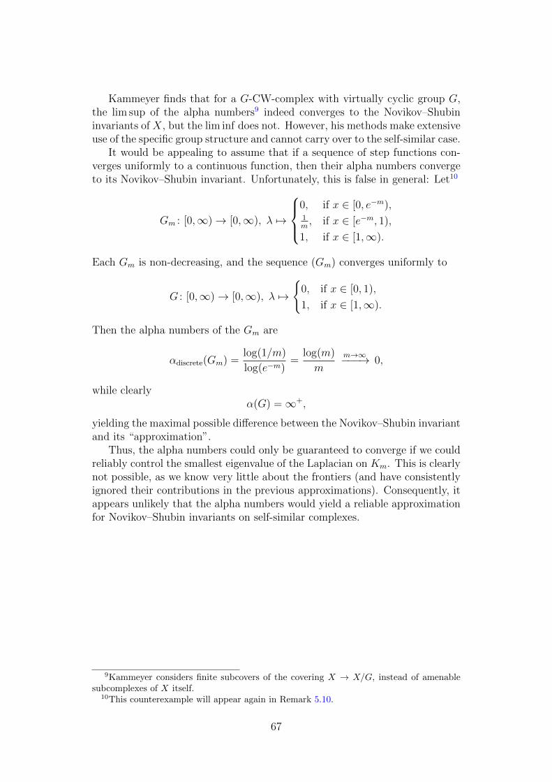
Kammeyer finds that for a G-CW-complex with virtually cyclic group G,the lim sup of the alpha numbers9 indeed converges to the Novikov–Shubininvariants of X, but the lim inf does not. However, his methods make extensiveuse of the specific group structure and cannot carry over to the self-similar case.
It would be appealing to assume that if a sequence of step functions con-verges uniformly to a continuous function, then their alpha numbers convergeto its Novikov–Shubin invariant. Unfortunately, this is false in general: Let10
Gm : [0,∞)→ [0,∞), λ 7→
0, if x ∈ [0, e−m),1m, if x ∈ [e−m, 1),
1, if x ∈ [1,∞).
Each Gm is non-decreasing, and the sequence (Gm) converges uniformly to
G : [0,∞)→ [0,∞), λ 7→
0, if x ∈ [0, 1),
1, if x ∈ [1,∞).
Then the alpha numbers of the Gm are
αdiscrete(Gm) =log(1/m)
log(e−m)=
log(m)
m
m→∞−−−→ 0,
while clearlyα(G) =∞+,
yielding the maximal possible difference between the Novikov–Shubin invariantand its “approximation”.
Thus, the alpha numbers could only be guaranteed to converge if we couldreliably control the smallest eigenvalue of the Laplacian on Km. This is clearlynot possible, as we know very little about the frontiers (and have consistentlyignored their contributions in the previous approximations). Consequently, itappears unlikely that the alpha numbers would yield a reliable approximationfor Novikov–Shubin invariants on self-similar complexes.
9Kammeyer considers finite subcovers of the covering X → X/G, instead of amenablesubcomplexes of X itself.
10This counterexample will appear again in Remark 5.10.
67
5 Fuglede–Kadison determinants and torsion
The Fuglede–Kadison determinant is, for the most part, a generalization of theusual determinant to operators on infinite-dimensional spaces, and it preservesseveral important properties of the determinant.
However, it deviates from the classical determinant in two regards: First,as its definition relies on the spectral density function of an operator, it onlydepends on the “absolute value” of the operator, and will never carry a sign.
Second, and most importantly, the Fuglede–Kadison determinant of anoperator ignores the operator’s kernel – especially, it does not become zerowhenever the operator is not injective! The determinant can become zero, butthis instead requires a large amount of very small spectral values. Thus, a zerodeterminant indicates a large “almost-kernel” instead of a non-trivial kernel.11
In the first part of this chapter, we will show that the Fuglede–Kadisondeterminants in our setting show most of the properties of their classical coun-terparts, especially multiplicativity. In the second part, we discuss whetherthese determinants can be approximated by finite-dimensional analogues. Thethird and last part of the chapter defines and briefly discusses the third L2-invariant, L2-torsion, that is constructed from the Fuglede–Kadison determi-nants of Laplacians.
5.1 Definition and properties
5.1 Definition. Given an operator T with spectral density function F T , definethe Fuglede–Kadison determinant of T by
detFK(T ) = exp
∫(0,∞)
log(λ) dF T (λ),
where we set exp(−∞) = 0 and the measure dF T is given by
dF T((a, b]
)= F T (b)− F T (a).
T is called of determinant class if detFK(T ) > 0, that is, if the integral in thedefinition is finite.
5.2 Remark. (a) As the definition of detFK(T ) only depends on the spectraldensity function of T , one can also speak of “the determinant of F” forany non-decreasing right-continuous function F : [0,∞)→ [0,∞).
(b) If T has eigenvalues, F T can have jump discontinuities, and thus themeasure dF T can have atoms. Especially, if T is not injective, it canhappen that dF T (0) > 0, so it is important to note that the domainof integration does not contain the point 0.
11Large “almost-kernels” correspond to small Novikov–Shubin numbers, and indeedα(T ) > 0 implies detFK(T ) > 0. See [Luc02], Theorem 3.14 (4).
68
(c) On the other hand, the upper bound of the domain of integration isirrelevant: For any λ > ‖T‖op, we have F T (λ) = trN (ET (λ)) = 1, so
dF T((‖T‖op ,∞
))= 0. Thus, the Fuglede–Kadison determinant can be
computed as
detFK(T ) = exp
∫(0,‖T‖op]
log(λ) dF T (λ).
For the practical computation of the Fuglede–Kadison determinant, thefollowing lemma is most useful:
5.3 Lemma ([Luc02], Lemma 3.15). If∫
(0,b]log(λ) dF (λ) > −∞, then∫
(0,b]
log(λ) dF (λ) = log(b)(F (b)− F (0)
)−∫ b
0
F (λ)− F (0)
λdλ.
To simplify notation, let
F⊥(λ) = F (λ)− F (0).
Then we obtain∫(0,b]
log(λ) dF (λ) = log(b)F⊥(b)−∫ b
0
F⊥(λ)
λdλ.
5.4 Remark. If T : Cn → Cn is a positive self-adjoint operator, then
detFK(T ) = n
√∏λ eigenvalue of T |λ > 0.
Especially, the Fuglede–Kadison determinant of an operator on a finite-dimen-sional space is never zero. (The determinant of the zero operator is given byan empty product, and thus it equals 1.)
Many properties of the Fuglede–Kadison determinant, most importantlytheir multiplicativity, carry over from the classical case.
In the following theorem, most statements and proofs follow Luck ([Luc02],Theorem 3.14 and Lemma 3.15), except for 5.5 (b):
5.5 Theorem. Always let S, T ∈ Nj(X).
(a) detFK(T ) = detFK(T ∗) =√
detFK(T ∗T ) =√
detFK(TT ∗).
(b) If T is self-adjoint, then T + P kerT is injective and
detFK(T + P kerT ) = detFK(T ).
(c) If T is positive and injective, then
detFK(T ) = limε→0+
detFK(T + ε id).
69
(d) If T is invertible, then
detFK(T ) = exp
(1
2trN(log(T ∗T )
)).
(e) If S, T are injective and positive, then
S ≤ T =⇒ detFK(S) ≤ detFK(T ).
(f) If S is injective and T has dense image, then
detFK(ST ) = detFK(S) detFK(T ).
Proof. (a) By Lemma A.8, every self-adjoint operator fulfills F T (λ) = F T 2(λ2),
and for every other operator T , the spectral density function is definedby F T (λ) = F T ∗T (λ2). Therefore, we get
dF T ∗T ((a, b]) = F T (√b)− F T (
√a) = dF T ((
√a,√b])
and thus
detFK(T ∗T ) = exp
∫(0,∞)
log(λ) dF T ∗T (λ)
= exp
∫(0,∞)
log(λ2) dF T (λ) = detFK(T )2
The same argument shows detFK(T ∗) =√
detFK(TT ∗), and applyingLemma 2.40 yields detFK(T ) = detFK(T ∗).
(b) Write T = T + PkerT . Given a vector z = x+ y ∈ ker(T )⊕ ker(T )⊥, we
have T z = x+ Ty and 〈x, Ty〉 =〈Tx, y〉 = 0. Therefore,∥∥∥T z∥∥∥2
= ‖x‖2 + ‖Ty‖2 ,
and this implies that the spectral density function of T is given by
F T (λ) =
F T (λ)− F T (0) if λ ∈ [0, 1),
F T (λ), if λ ∈ [1,∞).
Thus, the resulting measure on (0,∞) is given by
dF T = dF T + F T (0) · δ1,
and as log(1) = 0, this implies
detFK(T ) = exp
∫(0,∞)
log(λ) dF T (λ) = exp
∫(0,∞)
log(λ) dF T (λ) = detFK(T ).
70
(c) This follows from F T+εid(λ) = F T (λ − ε) and Beppo Levi’s monotoneconvergence theorem.
(d) If T and thus T ∗T are invertible, they are bounded from below, sospec(T ∗T ) ⊆ (0,∞) and log(T ∗T ) ∈ Nj. Applying part (a) and TheoremA.6 gives
log detFK(T ) =1
2log detFK(T ∗T )
=1
2
∫(0,∞)
log(λ) dF T ∗T (λ)
=1
2trN
∫(0,∞)
log(λ) dET ∗T (λ)
=1
2trN(log(T ∗T )
).
(e) From ∥∥∥√Sx∥∥∥2
=〈x, Sx〉 ≤〈x, Tx〉 =∥∥∥√Tx∥∥∥2
and Lemma 2.42, we get F√T (λ) ≤ F
√S(λ) for all λ ∈ [0,∞), and with
part (a), this yields F T (λ) ≤ F S(λ) for all λ ∈ [0,∞). Using Lemma 5.3with b = max
(‖S‖ , ‖T‖
), we have
log detFK(S) = log(b)F S(b)−∫ b
0
F S(λ)
λdλ
and the same for T . (Note that S, T are injective, so F S(0) = 0 = F T (0).)As F S(b) = dimN (`2(EjX)) = F T (b), this implies the result.
(f) Show first: If A,B are both positive and invertible, then
detFK(ABBA) = detFK(A)2 detFK(B)2.
Use Lemma 3.18 from [Luc02]: If the operator-valued functionX : [0, 1]→B(H) is differentiable (in the sense that there is X ′(t) ∈ B(H) such that1ε‖X(t+ ε)−X(t)− εX ′(t)‖op
ε→0−−→ 0), and if⋃t spec(X(t)) lies in the
interior of the domain of a holomorphic function f , then
trN
(d
dtf(X(t)
))= trN
(f ′(X(t)
)X ′(t)
).
Luck proves this for the von Neumann trace on N (G), but the only prop-erty of the trace his proof requires is that it commutes with integration,which holds for trN , too, as every integral
∫ 1
0X(t) dt fulfills by definition⟨
ξ1,
∫ 1
0
X(t) dt ξ2
⟩=
∫ 1
0
〈ξ1, X(t)ξ2〉 dt for all ξ1, ξ2 ∈ H.
71
As A,B > 0 are invertible, their spectra are contained in [ε,∞) forsome ε > 0, so log(A), log(B) and log(ABBA) are defined and bounded.Applying the previous lemma gives
d
dttrN
(log(A
(tB2 + (1− t)id
) A))
=d
dttrN
(log(tB2 + (1− t)id
)).
As for t = 0 we have
trN(log(A
(0 ·B2 + 1 · id
) A))
= trN(log(A2)
),
trN(log(0 ·B2 + 1 · id
))= 0,
this yields
trN(log(A B2 A)
)− trN
(log(A2)
)=
∫ 1
0
d
dttrN
(log(A
(tB2 + (1− t)id
) A))dt
=
∫ 1
0
d
dttrN
(log(tB2 + (1− t)id
))dt
= trN(log(B2)
)− trN (log(id))
= trN(log(B2)
).
Together with part (d), this implies detFK(ABBA) = detFK(A)2 detFK(B)2
for invertible A,B.
Now extend this statement to any injective A,B ≥ 0. Choose C > 0such that for all ε ∈ [0, 1],
ABBA ≤ A (B + ε id)2A ≤ ABBA+ C ε id.
Since ABBA ≥ 0 is injective, we can then use part (e) to get
limε→0+
detFK
(A (B + εid)2A
)= detFK(ABBA).
Setting X = BA in detFK(X∗X) = detFK(XX∗), we get det(ABBA) =det(BAAB), and so,
detFK(ABBA) = limε→0+
detFK
(A (B + ε id)2A
)= lim
ε→0+detFK
((B + ε id)A2 (B + ε id)
)= lim
ε→0+limδ→0+
detFK
((B + ε id) (A+ δ id)2 (B + ε id)
).
Now apply the previous result, as B + ε id and A+ δ id are positive andinvertible. This gives, for any injective A,B > 0,
detFK(ABBA) = limε→0+
detFK (B + ε id)2 limδ→0+
detFK (A+ δ id)2
= detFK(B)2 detFK(A)2.
72
Finally, return to the original statement. Let S be injective and T havedense image. Write S = V B and T = AU with U, V unitary and B =√S∗S, A =
√TT ∗ positive. Note that since T ∗ is injective, the operators
A and B are both injective. Thus, we can conclude
detFK(ST ) =√
detFK(T ∗S∗ST )
=√
detFK(U∗ABV ∗V BAU)
=√
detFK(U∗ABBAU)
=√
detFK(ABBA)
=√
detFK(A)2 detFK(B)2
= detFK(A) detFK(B)
= detFK(S) detFK(T ).
5.6 Remark. Even in the finite-dimensional case, properties (c), (e) and (f) failwithout injectivity: Simply consider S, T ∈ Mat2(C), where the trace is givenby
trN
(a bc d
)=a+ d
2
and thus the Fuglede–Kadison determinant is the square root of the productof the absolute values of the non-zero singular values of a matrix.
(c) Let T =
(1 00 0
). This is positive but not injective, and detFK(T ) = 1.
On the other hand, detFK(T + ε id) =√
(1 + ε) · ε ε→0−−→ 0.
(e) Let S =
(1 00 0
)and T =
(2 00 1/4
). Then we have S ≤ T , but
detFK(S) = 1 ≥ 1/√
2 = detFK(T ).
(f) Using the same example matrices as for (e), we have
detFK(ST ) =√
2 6= 1 · 1√2
= detFK(S) · detFK(T ).
To show that the “essential surjectivity” of the second operator (i. e.dense image) is also necessary, consider
detFK(TS) =√
2 6= 1√2· 1 = detFK(T ) · detFK(S).
If T ∈ Nj(X) is positive but not injective, 5.5 (c) can be generalized asfollows:
5.7 Corollary. Assume T ∈ Nj(X) and T ≥ 0, and let β := dimN (ker T ).Then
detFK(T ) = limε→0+
ε−β detFK(T + ε id).
73
Proof. Write P = PkerT for the orthogonal projection to ker(T ) ⊆ H. Abbrevi-ate β = dimN (ker T ) and η = dimN (Hj). (Under the standard normalization,η = 1, but the statement still holds for other normalizations.)
Combining 5.5 (b) and (c), we have
detFK(T ) = limε→0+
detFK(T + P + ε id).
Since TP = 0, we have (T + ε id)(ε−1P + id) = T + P + ε id, and as bothT + ε id and ε−1P + id are invertible for every ε > 0, we get from 5.5 (f)
detFK(T ) = limε→0+
(detFK(T + ε id) · detFK(ε−1P + id)
).
Finally, note that the spectral density function of ε−1P + id is given by
F ε−1P+id(λ) =
0 for λ ∈ [0, 1),
dimN (ker(T )⊥) = η − β for λ ∈ [1, 1 + ε−1),
dimN (Hj) = η for λ ∈ [1 + ε−1,∞),
which yields
detFK(ε−1P + id) = exp
∫(0,∞)
log(λ) dF ε−1P+id(λ)
= exp((η − β) log(1) + β log(1 + ε−1)
)= (1 + ε−1)β.
For ε→ 0+, this is asymptotically equal to ε−β, and therefore,
detFK(T ) = limε→0+
(detFK(T+ε id) detFK(ε−1P+id)
)= lim
ε→0+ε−β detFK(T+ε id).
The most interesting determinants are those of Laplacians. In the classi-cal case, Dodziuk and Mathai ([DM98]) showed that Laplacians on G-CW-complexes are always of determinant class, and their proof can be adapted tothe self-similar case as well:
5.8 Theorem. The Laplacians ∆(X)j of a self-similar CW-complex X are of
determinant class.
Proof. Show first that detFK
(∆
(Km)j
)≥ 1 for every m.
Let k = dimC ker(∆
(Km)j
)and let λ1, . . . , λr be the eigenvalues of ∆
(Km)j ,
where λi = 0 for i ≤ k and λi > 0 for i > k. As mentioned in Remark 5.4,
detFK
(∆
(Km)j
)= r
√√√√ r∏i=k+1
λi > 0.
74
The characteristic polynomial of ∆(Km)j is
χ(x) =r∏i=1
(λi − x) = xk ·r∏
i=k+1
(λi − x) =: (−x)k · ψ(x).
Note thatψ(0) = detFK
(∆
(Km)j
)r> 0.
Since this can also be computed as
χ(x) = det(
∆(Km)j − x · id
)and ∆
(Km)j is an integer matrix, we know that χ(x) has integer coefficients,
and so the same must hold for ψ(x)! Therefore, ψ(0) > 0 implies ψ(0) ≥ 1,and this proves the claim.
Now let Fm be the normalized spectral density function of ∆(Km)j . Choose
b > 0 large enough that∥∥∥∆
(X)j
∥∥∥ ≤ b and∥∥∥∆
(Km)j
∥∥∥ ≤ b for all m. (This is
possible since the bound on the norm of the Laplacian only depends on thenumber of “neighbors” a cell can have, which is bounded throughout X.) Weget for all m
log detFK(Fm) = log detFK
(∆
(Km)j
)≥ 0.
On the other hand,
log detFK(Fm) = log(b)F⊥m(b)−∫
(0,b]
F⊥m(λ)
λdλ,
so for all m
log(b)F⊥m(b) ≥∫
(0,b]
F⊥m(λ)
λdλ.
Since Fm converges pointwise12 to F = F(∆
(X)j
), there is M ∈ N such that for
all m ≥M ,
log(b)F⊥(b) ≥∫
(0,b]
F⊥m(λ)
λdλ.
Now, Fatou’s lemma gives
log(b)F⊥(b) ≥∫
(0,b]
F⊥(λ)
λdλ,
and therefore
log detFK(F ) = log(b)F⊥(b)−∫
(0,b]
F⊥(λ)
λdλ ≥ 0.
12Even uniformly, but we don’t need that here.
75
5.2 Approximation
Let us explore under which circumstances the Fuglede–Kadison determinantsof geometric operators can be approximated by finite-dimensional restrictions.13
By Theorem 3.11, the spectral density function of an operator T on a self-similar complex is approximated uniformly by those of restrictions of T to finitesubcomplexes Km. Recalling Lemma 5.3, we can express the determinants asfollows (with F⊥(λ) = F (λ)− F (0) and b ≥ ‖T‖):
log detFK(F ) = log(b)F⊥(b)−∫
(0,b]
F⊥(λ)
λdλ.
However, as 1/λ is unbounded on (0, b], even uniform convergence Fm → Fwill not ensure convergence of these integrals.
This problem can of course be avoided if the domain of integration isbounded away from zero. This is satisfied when T has a spectral gap at zero:
5.9 Theorem. Let X be a self-similar complex with Følner sequence (Km).Assume that T ∈ Aj(X) is positive and has a spectral gap at zero, that is,spec(T ) ∩ (0, ε) = ∅ for some ε > 0. (This is equivalent to T being invertiblewhen restricted to ker(T )⊥.)
Define Tm := PmTIm, where Im : `2(EjKm)→ `2(EjX) is the inclusion andPm : `2(EjX)→ `2(EjKm) is the orthogonal projection. Then
detFK(T ) = limm→∞
detFK Tm.
Proof. Note first that the spectrum of T does not depend on whether weconsider it as an element of B(`2(EjX)) or an element of B(Hj(X)).
By assumption, there is ε > 0 such that
〈v, Tv〉 ≥ ε ‖v‖2 for all v ∈ ker(T )⊥ ⊆ `2(EjX).
Using P ∗m = Im, we have
〈w, Tmw〉 =〈w,PmTImw〉 =〈w, Tw〉 for all w ∈ `2(EjKm),
so ker(Tm) = ker(T ) ∩ `2(EjKm), and we obtain
〈w, Tmw〉 =〈w, Tw〉 ≥ ε ‖w‖2 for all w ∈ ker(Tm)⊥ ⊆ `2(EjKm).
Consequently, both F T and every F Tm are constant on [0, ε). Furthermore,note that ‖Tm‖ ≤ ‖T‖ for all m. As the function λ 7→ 1/λ is bounded on[ε,∞), uniform convergence F Tm → F T implies convergence of the integrals∫
[ε,‖T‖]
F Tm(λ)
λdλ
m→∞−−−→∫
[ε,‖T‖]
F T (λ)
λdλ.
By Lemma 5.3, the claim follows.
13In the classical case, the approximation of Fuglede–Kadison determinants of any oper-ator T ∈ Matr,s(QG) is known if G is an infinite virtually cyclic group. For G = Zn it isknown that detFK(T ) = lim supm detFK(Tm). See [Luc16], Remark 6.5.
76
In this lemma, we have used that a spectral gap of T directly implies thatthe restrictions of T to smaller subcomplexes have the exact same spectralgap. This would not necessarily work with the more general “approximatingoperators” in Theorem 3.11, as a single “rogue eigenvalue” getting too closeto zero can destroy the convergence:
5.10 Example. Define a sequence of functions
Gm : [0,∞)→ [0,∞), λ 7→
0, if x ∈ [0, e−m),1m, if x ∈ [e−m, 1),
1, if x ∈ [1,∞).
Each Gm is non-decreasing, and the sequence (Gm) converges uniformly to
G : [0,∞)→ [0,∞), λ 7→
0, if x ∈ [0, 1),
1, if x ∈ [1,∞).
Yet, one clearly has for all m ∈ N
log detFK(Gm) = log(1)Gm(1)−∫ 1
0
Gm(λ)
λdλ
= 0−∫ 1
e−m
1
mλdλ
= − log(1)− log(e−m)
m= −1,
log detFK(G) = log(1)G(1)−∫ 1
0
G(λ)
λdλ
= 0,
and thus
detFK(Gm) =1
e6−→ 1 = detFK(G).
More generally, for any bounded non-decreasing function F : [0,∞)→ [0,∞),
define a sequence of functions Fm = F +Gm. Then each Fm is non-decreasing,the sequence (Fm) converges uniformly to the function F = F +G, and, sincelog detFK(F ) is linear in the function F ,
limm→∞
log detFK(Fm) = log detFK(F )− 1.
If the functions in counterexample 5.10 were indeed the spectral densityfunctions of a sequence of operators, the lowest “eigenvalue” of those operatorswould have to decay exponentially in m, while their normalized multiplicitydecayed only polynomially (indicating that the number of cells in Km increasedpolynomially in m). This indicates that the convergence of determinants might
77
be achievable in cases where the smallest positive eigenvalues of the restrictionsTm can be controlled:
Assume that T ∈ Aj(X) is of determinant class but without spectral gap,and let Tm, Fm and F be as above. Abbreviate εm = ‖Fm − F‖∞ and let µmbe the smallest positive eigenvalue of Tm. Since T has no spectral gap and Fmapproximates F , we know that
limm→∞
εm = 0 = limm→∞
µm.
Since F⊥m(λ) = 0 for λ < µm, we obtain the estimate∣∣∣∣∫ b
0
F⊥(λ)− F⊥m(λ)
λdλ
∣∣∣∣ ≤ ∫ µm
0
F⊥(λ)
λdλ+
∫ b
µm
εmλ
dλ
≤∫ µm
0
F⊥(λ)
λdλ+ εm · (log(b)− log(µm)) .
Since F is of determinant class, we know that∫ µm
0
F⊥(λ)
λdλ
µm→0−−−→ 0,
and obviouslyεm log(b)
m→∞−−−→ 0.
Therefore, detFK(Tm) will converge to detFK(T ) if
εm log(µm)m→∞−−−→ 0.
This would be satisfied if µm were bounded from below by any power of εm.The proof of 3.11 shows that
εm := ‖Fm − F‖∞ = O(|FjKm||EjKm|
).
Thus, εm falls faster if the complex is “more amenable”.The problem of bounding this smallest positive eigenvalue has been studied
extensively for the Laplacians of graphs. However, the answer points in thewrong direction for our purpose: The smallest positive eigenvalue becomes“large”, when the graph is a magnifier , that is, all subsets of the graph have“large” neighborhoods. In other words, we obtain a better bound on thesmallest eigenvalue if the complex is less amenable! More concretely, considerthe following result by Alon:
5.11 Lemma ([Alo86], Lemma 2.4). If K is a finite graph such that everyvertex subset A ⊆ E0K with |A| ≤ 1
2|E0K| fulfills
|σ ∈ E0K | dcomb(σ,A) = 1| ≥ c |A|
for some constant c > 0, then the smallest positive eigenvalue of ∆(K)0 is at
least c2/(2c2 + 4).
78
For well-chosen Følner sequences (Km), these two properties can sometimesbe reconciled. Essentially, this requires an exhaustion (Km) such that no Km
has a proper subset that is “much more amenable” than Km itself:
5.12 Theorem. Let X be a self-similar complex and assume there is a self-similar Følner sequence (Km) for which there are constants c, e > 0 such thatfor every vertex subset Am ⊆ E0Km with |A| ≤ 1
2|E0Km|,
|σ ∈ E0Km | dcomb(σ,A) = 1||A|
≥ c ·(|FjKm||EjKm|
)e.
Thenlimm→∞
detFK
(∆
(Km)0
)= detFK
(∆
(X)0
).
Proof. Use the same notation as above. (Note, however, that unlike in The-
orem 5.9, ∆(Km)0 is not the restriction of ∆
(X)0 to Km.) By Alon’s lemma and
Theorem 3.11, we have µm ≥ d c2ε2em , where d > 0 combines the factor 4 from
5.11 with the O-constant of εm = O(|FjKm||EjKm|
), and that gives
|εm log µm| ≤∣∣εm · (log(dc2) + 2e log(εm)
)∣∣ m→∞−−−→ 0.
5.13 Example. (a) Consider the Laplacian on one-cells of Rd with the stan-dard CW-structure (compare Example 3.2), and choose a Følner se-quence consisting of cubes, Km = [−3m, 3m]d. We obtain
εm ∼|FjKm||EjKm|
∼ 1
3m
On the other hand, among subsets A ⊆ E0Km with |A| ≤ 12|E0Km|, the
one with the fewest frontiers in Km will simply be a half-cube, containing12· (2 · 3m)d vertices, of which (2 · 3m)d−1 are frontiers, so 5.11 yields a
lower bound
µm ≥( c
3m
)2
for some constant c > 0. This easily suffices to ensure convergence ofdeterminants.
(b) For Sierpinski’s triangle (see Example 3.3), there are numerous sub-complexes of any size with exactly three frontiers (namely, large sub-triangles). Thus, the constant c in 5.11 frequently takes values pro-portional to 1/ |A|, but one can also choose (Km) in such a way thatεm ∼ 1/ |E0Km|. Again, we obtain µm ∼ ε2
m, which suffices for conver-gence.
79
5.3 L2-torsion
The Fuglede–Kadison determinants of Laplacians of a space are not homotopyinvariants by themselves.14 However, they give a rise to another L2-invariant,the L2-torsion.
Classically, L2-torsion is defined as the logarithm of the alternating productof Fuglede–Kadison determinants of the differentials ∂
(X)j . This is easily shown
to be equal to the following expression in terms of the Laplacians, which shallserve as our definition:
5.14 Definition. The L2-torsion of an aperiodically ordered CW-complex Xis
ρ(2)(X) = −1
2
dimX∑j=0
(−1)j · j · log detFK
(∆
(X)j
),
provided every ∆(X)j is of determinant class.
This definition makes sense for any self-similar complex, as their Laplaciansare always of determinant class (see 5.8).
Whether the L2-torsion is in fact a homotopy invariant remains a difficultquestion. In the classical case, this can be proven for G-CW-complexes thatare “det-L2-acyclic”, that is, where every Laplacian is of determinant class andall L2-Betti numbers vanish:
5.15 Theorem ([Luc02], Theorem 3.93 and Lemma 13.6). Let X and Y befinite free G-CW-complexes, where G is an amenable group. If X and Y areG-homotopy equivalent and one of the two is det-L2-acyclic, then both of themare det-L2-acyclic and ρ(2)(X) = ρ(2)(Y ).
Unfortunately, proving an analogous statement for the self-similar case isbeyond the scope of this thesis: In the classical case, the L2-torsion of X and Ywill a priori differ by a term related to the Whitehead torsion of the homotopyequivalence between the two; the classical proof then relies on properties ofthe group G to ensure that this term (always) vanishes. In the aperiodicalcase, no such Whitehead torsion exists; it remains to be determined if there isa suitable analogue.
As an additional complication, even if the L2-Betti numbers vanish, theL2-chain complex of a self-similar complex may not be truly L2-acyclic, sincesome Laplacians may have (small) kernels in `2(EjX) even if the induced op-erators on Hj(X) are injective. Finally, there can be no finite-dimensionalanalogue that carries over to the whole space by approximation, as the usual(non-L2) chain complex of a finite CW-complex cannot be acyclic.
14Finite example: In a circle formed from three 0-cells and three 1-cells, we havedetFK(∆1) = 3
√9 ≈ 2.08, while in a circle with four 0-cells and four 1-cells, detFK(∆1) =
4√
16 = 2.
80
6 Product spaces
Intuitively, the cartesian product of two self-similar spaces should again be aself-similar space. That is indeed the case (although it takes a nonzero amountof work to prove amenability), and thus, it makes sense to try and express theL2-invariants of such a product space through those of its factors. In this finalchapter, we will derive such formulas for L2-Betti numbers, Novikov–Shubininvariants and L2-torsion.
In doing so, we hope to demonstrate once more how the approximationtheorem for spectral density functions allows us to gain information aboutL2-invariants, even when those invariants themselves cannot be approximatedby finite-dimensional analogues.
6.1 Products of self-similar complexes are self-similar
6.1 Theorem. Let X and Y be self-similar CW-complexes with self-similarexhaustions (Km) respectively (Lm). Then X×Y is a self-similar CW-complexwith self-similar exhaustion (Km × Lm).
Proof. Note first that the product of regular CW-complexes is again regu-lar: For any two cells σ ∈ EjX and τ ∈ EkY , the extended attaching maps
fσ : Dj → σ ⊆ X and fτ : Dk → τ ⊆ Y are by assumption homeomorphisms,
so the product attaching map fσ×τ : Dj+k ≈ Dj ×Dk fσ×fτ−−−→ σ × τ ⊆ X × Yis again a homeomorphism.
Second, the product of bounded complexes is bounded: The topologicalboundary of a product cell is ∂(σ × τ) = ∂σ × τ ∪ σ × ∂τ , and thus we get
|κ ∈ Ej+k−1(X × Y ) |κ ⊆ ∂(σ × τ)|
=∑
a+b=j+k−1
|λ× µ ∈ EaX × EbY |λ ⊆ σ, µ ⊆ τ)|
≤ |λ ∈ E∗X |λ ⊆ σ| · |µ ∈ E∗Y |µ ⊆ τ)|
and analogously
|κ ∈ Ej+k+1(X × Y ) | (σ × τ) ⊆ ∂κ|≤∣∣λ ∈ E∗X ∣∣σ ⊆ λ
∣∣ · |µ ∈ E∗Y | τ ⊆ µ)|
where E∗X =⋃j EjX is the set of all cells of X. As X and Y are bounded,
these numbers are bounded, showing that X × Y is bounded.To show that (Km×Lm) is again a Følner sequence, we need to understand
the frontiers in a product space:
6.2 Lemma. Let X, Y be regular CW-complexes. Let σ1 ∈ Ej1X, σ2 ∈ Ej2X,τ1 ∈ Ek1Y and τ2 ∈ Ek2Y such that j1 +k1 = d = j2 +k2. Then the cells σ1× τ1
and σ2× τ2 are adjacent in Ed(X×Y ) if and only if one of the following holds:
81
(a) (j1, k1) = (j2, k2), σ1 is adjacent to σ2 in X and τ1 = τ2.
(b) (j1, k1) = (j2, k2), σ1 = σ2 and τ1 is adjacent to τ2 in Y .
(c) (j1, k1) = (j2 + 1, k2 − 1), ∂σ1 ⊇ σ2 and τ1 ⊆ ∂τ2.
(d) (j1, k1) = (j2 − 1, k2 + 1), σ1 ⊆ ∂σ2 and ∂τ1 ⊇ τ2.
Proof. [⇐=] follows immediately from ∂(σ × τ) = (∂σ × τ) ∪ (σ × ∂τ).[=⇒]: Assume that σ1 × τ1 and σ2 × τ2 share a (j1 + k1 − 1)-face σ3 × τ3:
σ3 × τ3 ⊆ ∂(σ1 × τ1) ∩ ∂(σ2 × τ2)
= ((∂σ1 × τ1) ∪ (σ1 × ∂τ1)) ∩ ((∂σ2 × τ2) ∪ (σ2 × ∂τ2))
= ((∂σ1 × τ1) ∩ (∂σ2 × τ2)) ∪ ((∂σ1 × τ1) ∩ (σ2 × ∂τ2))
∪ ((σ1 × ∂τ1) ∩ (∂σ2 × τ2)) ∪ ((σ1 × ∂τ1) ∩ (σ2 × ∂τ2))
= ((∂σ1 ∩ ∂σ2)× (τ1 ∩ τ2)) ∪ ((∂σ1 ∩ σ2)× (τ1 ∩ ∂τ2))
∪ ((σ1 ∩ ∂σ2)× (∂τ1 ∩ τ2)) ∪ ((σ1 ∩ σ2)× (∂τ1 ∩ ∂τ2))
By Lemma 2.2, σ3×τ3 must be fully contained in one of the four “∪-summands”.For purely dimensional reasons (and because any two open cells are either iden-tical or disjoint),
σ3 × τ3 ⊆ (∂σ1 ∩ ∂σ2)× (τ1 ∩ τ2) implies case (a),σ3 × τ3 ⊆ (∂σ1 ∩ σ2)× (τ1 ∩ ∂τ2) implies case (c),σ3 × τ3 ⊆ (σ1 ∩ ∂σ2)× (∂τ1 ∩ τ2) implies case (d),σ3 × τ3 ⊆ (σ1 ∩ σ2)× (∂τ1 ∩ ∂τ2) implies case (b).
Conversely, assume there is a (j1 +k1 +1)-cell σ4×τ4 whose boundary containsboth σ1 × τ1 and σ2 × τ2:
(σ1 × τ1) ∪ (σ2 × τ2) ⊆ (∂σ4 × τ4) ∪ (σ4 × ∂τ4)
Using Lemma 2.2 again, each of the two σi× τi must be contained in ∂σ4× τ4
or in σ4 × ∂τ4. We obtain the following cases:(σ1 × τ1) ∪ (σ2 × τ2) ⊆ ∂σ4 × τ4 implies case (a),(σ1 × τ1) ∪ (σ2 × τ2) ⊆ σ4 × ∂τ4 implies case (b),σ1 × τ1 ⊆ ∂σ4 × τ4 and σ2 × τ2 ⊆ σ4 × ∂τ4 implies case (d),σ1 × τ1 ⊆ σ4 × ∂τ4 and σ2 × τ2 ⊆ ∂σ4 × τ4 implies case (c).
Proof of Theorem 6.1, continued. Let G(m,m + 1) and G ′(m,m + 1) be thesets of local isomorphisms for X resp. Y associated to the Følner sequences(Km) and (Lm). It is clear that
Km+1 × Lm+1 =⋃
γ ∈G(m,m+1)
δ ∈G′(m,m+1)
(γ × δ)(Km × Lm).
It remains to show that the exhaustion (Km × Lm) is amenable (i. e. a Følnersequence).
82
Let σ1 ∈ EjX and τ1 ∈ EkY such that σ1 × τ1 is a frontier of Km × Lm.Let σ2× τ2 be a cell of (X × Y ) \ (Km×Lm) adjacent to it and apply Lemma6.2. Case (a) implies σ1 ∈ FjKm and case (b) implies τ1 ∈ FkLm. In case(c), σ2 ⊆ ∂σ1 ⊆ Km, so τ2 6⊆ Lm. As Lm is a full subcomplex, τ2 must havea face outside Lm, and that face is adjacent (via τ2) to τ1, so τ1 ∈ FkLm.Analogously, we get σ1 ∈ FjKm in case (d). Thus, we obtain indeed
|Fd(Km × Lm)||Ed(Km × Lm)|
≤∑
j+k=d |(FjKm × EkLm) ∪ (EjKm ×FkLm)|∑j+k=d |EjKm × EkLm|
≤∑j+k=d
|(FjKm × EkLm) ∪ (EjKm ×FkLm)||EjKm × EkLm|
≤∑j+k=d
(|FjKm × EkLm||EjKm × EkLm|
+|EjKm ×FkLm||EjKm × EkLm|
)=∑j+k=d
(|FjKm||EjKm|
+|FkLm||EkLm|
)m→∞−−−→ 0.
6.2 L2-Betti numbers of product spaces
If K and L are finite CW-complexes, then K×L is a finite CW-complex whose`-cells are given by
E`(K × L) ∼=⋃
j+k=`
EjK × EkL.
And in perfect analogy, their (non-normalized) Betti numbers are given by theKunneth formula
β`(K × L;C) =∑j+k=`
βj(K;C) · βk(L;C).
Until now, we have usually normalized the trace on `2(EjX) = C[EjX] by thenumber of j-cells themselves (such that the trace becomes a state). Unfortu-nately, this normalization is incompatible with the Kunneth formula:
β`(K × L;C)
|E`(K × L)|=
∑j+k=` βj(K;C) · βk(L;C)∑
j+k=` |EjK × EjL|6=∑j+k=`
βj(K;C)
|EjK|· βj(K;C)
|EkL|
Getting the Kunneth formula to work with our approximation therefore re-quires a different normalization. The easiest solution is to always normalizeby the number of vertices instead: As a zero-cell in K×L must be the productof two zero-cells of K and L, we have
|E0(K × L)| = |E0K| · |E0L| ,
and thus the renormalized Kunneth formula holds:
β`(K × L;C)
|E0(K × L)|=∑j+k=`
βj(K;C)
|E0K|· βj(K;C)
|E0L|
83
Now, the approximation theorem for L2-Betti numbers yields a Kunnethformula for self-similar complexes:
6.3 Theorem. Let X and Y be self-similar complexes, and normalize everytrace by the numbers of vertices. Then L2-Betti numbers fulfill the Kunnethformula:
b(2)` (X × Y ) =
∑j+k=`
b(2)j (X) · b(2)
k (Y ).
Proof. Let (Km) and (Lm) be Følner sequences for X resp. Y . By Theorem6.1, (Km × Lm) is a Følner sequence for X × Y , and Corollary 4.2 togetherwith Lemma 3.17 gives us
b(2)` (X × Y ) = lim
m→∞
β`(Km × Lm)
|E0(Km × Lm)|=∑j+k=`
limm→∞
βj(Km)
|E0Km|· limm→∞
βk(Lm)
|E0Lm|
=∑j+k=`
b(2)j (X) · b(2)
k (Y ).
6.3 Novikov–Shubin invariants of product spaces
While there is no approximation theorem for Novikov–Shubin invariants, wecan make use of the approximation theorem for the spectral density functionsthemselves to obtain a formula for the Novikov–Shubin invariants of a productspace.
For any two finite subcomplexes K,L, the Laplacian of the product is givenby
∆(K×L)` =
⊕j+k=`
(∆
(K)j ⊗ id`2(EkL) + id`2(EjK) ⊗∆
(L)k
),
and for the non-normalized spectral density functions of operators on finite-dimensional spaces, we have
Fnn(f ⊕ g) = Fnn(f) + Fnn(g)
and (compare [Luc02], Lemma 2.31)
Fnn(f)(λ/2) ·Fnn(g)(λ/2) ≤ Fnn(f ⊗ id + id⊗ g)(λ) ≤ Fnn(f)(λ) ·Fnn(g)(λ).
Therefore, the non-normalized spectral density function of ∆(K×L)` fulfills
Fnn
(∆
(K×L)`
)'∑j+k=`
Fnn
(∆
(K)j
)· Fnn
(∆
(L)k
),
where the dilational equivalence only dilates by a factor of 2.This still holds if we normalize with the number of vertices, as |E0(K × L)| =
|E0K|·|E0L|, and as the dilatational equivalence uses the same constant (namely,2) for every subcomplex, the approximation theorem 3.11 yields
F(∆
(X×Y )`
)'∑j+k=`
F(∆
(X)j
)· F(∆
(Y )k
).
84
Finally, Lemma 4.7 gives α(F+G) = min(α(F ), α(G)
), and therefore we arrive
at the following statement, analogous to [Luc02], Lemma 2.35 (1):
6.4 Lemma. Let X and Y be self-similar complexes. Then
α`(X × Y ) = minj+k=`
α(F(∆
(X)j
)· F(∆
(Y )k
)).
It remains to express α(F · G) in terms of α(F ) and α(G). Recalling thenotation F⊥(λ) = F (λ)− F (0), we have
α(F ·G) = α(F⊥ ·G⊥ + F⊥ ·G(0) + F (0) ·G⊥ + F (0) ·G(0)
)= min
α(F⊥ ·G⊥), α(F⊥ ·G(0)), α(F (0) ·G⊥), α(F (0) ·G(0))
The constant function F (0) ·G(0) has α =∞+, so the last term is irrelevant.The middle terms can be relevant, depending on F (0) and G(0):
α(F⊥ ·G(0)) =
α(F⊥) = α(F ) if G(0) > 0,
∞+ if G(0) = 0.
α(F (0) ·G⊥) =
α(G⊥) = α(G) if F (0) > 0,
∞+ if F (0) = 0.
The first term is always relevant, but not always obvious: We have
α(F⊥ ·G⊥) = lim infλ→0
log(F⊥(λ) ·G⊥(λ))
log(λ)= lim inf
λ→0
log(F⊥(λ)) + log(G⊥(λ))
log(λ),
but a limit inferior, unlike a true limit, does not necessarily commute withaddition!
Thus, the final theorem about Novikov–Shubin invariants of product spacesis only guaranteed to be true if the complexes fulfill the limit property (seeRemark 4.6). Fortunately, the arguments outlined above also show that if Xand Y have the limit property, then so does X × Y .
6.5 Theorem. Let X and Y be self-similar complexes satisfying the limitproperty. Then
α`(X × Y ) = min
(αj(X) + αk(Y ) | j + k = `
∪αj(X)
∣∣∣ b(2)`−j(Y ) > 0
∪αk(Y )
∣∣∣ b(2)`−k(X) > 0
)Unlike in Theorems 6.3 and 6.6, the choice of normalization does not ac-
tually matter in this theorem, since replacing a spectral density function F byr · F for any constant r > 0 does not change the Novikov–Shubin invariant ofF (compare Lemma 4.7).
85
6.4 L2-torsion of product spaces
Finally, we aim to prove the following formula for the L2-torsion of a productspace:
6.6 Theorem. Let X and Y be self-similar complexes, and normalize everytrace by the numbers of vertices. Then
ρ(2)(X × Y ) = χ(2)(X) ρ(2)(Y ) + χ(2)(Y ) ρ(2)(X),
where χ(2) denotes the L2-Euler characteristic.
Although the torsion of X × Y is not necessarily equal to the limit of thetorsions of Km × Lm, it is worth it to prove this formula for finite complexesfirst – every lemma in the following subsection will be needed for the proof ofTheorem 6.6.
Torsion in the finite-dimensional case
6.7 Definition. Let (C∗, c∗) be a finite-dimensional chain complex of C-vectorspaces (i. e. all but finitely many Cp are 0, and the non-zero ones are finite-
dimensional). Define the Laplacians of C∗ by ∆(C)p = cp+1c
∗p+1 + c∗pcp, and let
F(∆
(C)p
)be their (non-normalized) spectral density functions.15 Then define
the torsion of C∗ by
ρ(C∗) = −1
2
∑p
(−1)p · p · log detFK F(∆(C)p
).
6.8 Theorem. Let C∗ and D∗ be chain complexes as above. Then
ρ(C∗ ⊗D∗) = χ(C∗) ρ(D∗) + χ(D∗) ρ(C∗).
The proof of this builds on two main lemmas. The first one explains whythe Euler characteristic appears in the formula:
6.9 Lemma. Let C∗ be a chain complex as above. Then∑p
(−1)pF(∆(C)p
)= χ(C∗) · χ[0,∞).
Proof. We have an orthogonal decomposition
Cp = ker ∆Cp ⊕ im(cp+1)⊕ ker(cp)
⊥.
Define c⊥p : ker(cp)⊥ → im(cp) as the restriction of cp. Then the Laplacian
decomposes as∆(C)p = 0⊕ c⊥p+1(c⊥p+1)∗ ⊕ (c⊥p )∗c⊥p
15While we are dealing purely with the finite-dimensional case, the non-normalized spec-tral density functions will simply be denoted F instead of Fnn.
86
Therefore, and because F (f ∗f) = F (ff ∗),
F(∆(C)p
)= dim
(ker ∆C
p
)· χ[0,∞) + F
(c⊥p+1(c⊥p+1)∗
)+ F
((c⊥p )∗c⊥p
)= βp(C∗) · χ[0,∞) + F
((c⊥p+1)∗c⊥p+1
)+ F
((c⊥p )∗c⊥p
).
This gives∑p
(−1)pF(∆(C)p
)=∑p
(−1)pβp(C∗) · χ[0,∞) +∑p
(−1)pF((c⊥p+1)∗c⊥p+1
)+∑p
(−1)pF((c⊥p )∗c⊥p
)= χ(C∗) · χ[0,∞) −
∑p
(−1)pF((c⊥p )∗c⊥p
)+∑p
(−1)pF((c⊥p )∗c⊥p
)= χ(C∗) · χ[0,∞).
The second main lemma expresses spectral density functions of the productcomplex via spectral density functions of the two “factors”:
6.10 Lemma. Let C∗ and D∗ be chain complexes as above. Then
F(∆(C⊗D)n
)=∑p+q=n
d
dλF(∆(C)p
)∗ F(∆(D)q
),
where ∗ denotes convolution.
Proof. Note first:
χ[µ,∞) ∗ χ[ν,∞)(λ) =
∫ +∞
−∞χ[µ,∞)(ξ) · χ[ν,∞)(λ− ξ) dξ
=
∫ +∞
−∞χ[µ,∞)(ξ) · χ(−∞,λ−ν](ξ) dξ
=
λ− µ− ν, if λ ≥ µ+ ν,
0, if λ ≤ µ+ ν,
and therefore, for almost all λ,
d
dλχ[µ,∞) ∗ χ[ν,∞)(λ) =
1, if λ > µ+ ν,0, if λ < µ+ ν,
= χ[µ+ν,∞)(λ).
By definition, the tensor product of chain complexes has the form
(C ⊗D)n =⊕p+q=n
Cp ⊗Dq
and it is known that
∆(C⊗D)n =
⊕p+q=n
(∆(C)p ⊗ idDq + idCp ⊗∆(D)
q
),
87
which immediately implies
F(∆(C⊗D)n
)=∑p+q=n
F(∆(C)p ⊗ idDq + idCp ⊗∆(D)
q
).
Define mp = dim(Cp) and nq = dim(Dq). Let (µp,i)mpi=1 be the eigenvalues
of ∆(C)p and (νq,j)
nqj=1 be the eigenvalues of ∆
(D)q . Then the eigenvalues of
∆(C)p ⊗ idDq + idCp ⊗∆
(D)q are exactly (µp,i + νq,j)i,j, and we obtain
∑p+q=n
d
dλF(∆(C)p
)∗ F(∆(D)q
)=∑p+q=n
d
dλ
(mp∑i=1
χ[µp,i,∞) ∗nq∑j=1
χ[νq,j ,∞)
)
=∑p+q=n
mp∑i=1
nq∑j=1
d
dλ
(χ[µp,i,∞) ∗ χ[νq,j ,∞)
)=∑p+q=n
mp∑i=1
nq∑j=1
χ[µp,i+νq,j ,∞)
=∑p+q=n
F(∆(C)p ⊗ idDq + idCp ⊗∆(D)
q
)= F
(∆(C⊗D)n
).
Now we are ready for the proof of Theorem 6.8. Unlike the lemmas, thisproof will not be needed to prove Theorem 6.6; but it uses the same methodsand can largely serve as a blueprint for the proof of that theorem.
Proof of Theorem 6.8. Choose b > a > 0 such that b > µp,i + νq,j hold forall p, q, i, j and µp,i > a, νq,j > a holds whenever µp,i > 0, νq,j > 0. (This ispossible since C∗ and D∗ are finite-dimensional.)
Start by using the linearity of the determinant:
ρ(C∗ ⊗D∗) = −1
2
∑n
(−1)n · n · log detFK
(∆(C⊗D)n
)= −1
2log detFK
(∑n
(−1)n · n · F(∆(C⊗D)n
))
(Note that only finitely many terms in the sum are non-zero.)Now compute this sum of spectral density functions using Lemma 6.9:∑
n
(−1)n · n · F(∆(C⊗D)n
)=∑n
(−1)n · n ·∑p+q=n
d
dλF(∆(C)p
)∗ F(∆(D)q
)=
d
dλ
∑p
(−1)pF(∆(C)p
)∗∑q
(−1)q · q · F(∆(D)q
)+
d
dλ
∑p
(−1)p · p · F(∆(C)p
)∗∑q
(−1)qF(∆(D)q
)88
=d
dλ
(χ(C∗) · χ[0,∞)
)∗∑q
(−1)q · q · F(∆(D)q
)+
d
dλ
∑p
(−1)p · p · F(∆(C)p
)∗(χ(D∗) · χ[0,∞)
)As in the proof of Lemma 6.10, we have
d
dλχ[µ,∞) ∗ χ[0,∞)(λ) =
d
dλχ[0,∞) ∗ χ[µ,∞)(λ) = χ[µ,∞)(λ)
for all µ and almost all λ (namely, λ 6= µ). Since F(∆
(C)p
)and F
(∆
(D)q
)are
linear combinations of such step functions, we get for almost all λ∑n
(−1)n · n · F(∆(C⊗D)n
)= χ(C∗) ·
∑q
(−1)q · q · F(∆(D)q
)+ χ(D∗) ·
∑p
(−1)p · p · F(∆(C)p
).
Again by linearity of log detFK, we obtain the claim:
ρ(C∗ ⊗D∗) = −1
2log detFK
(∑n
(−1)n · n · F(∆(C⊗D)n
))= χ(C∗) ·
(−1
2
)∑q
(−1)q · q · log detFK F(∆(D)q
)+ χ(D∗) ·
(−1
2
)∑p
(−1)p · p · log detFK
(F(∆(C)p
))= χ(C∗) ρ(D∗) + χ(D∗) ρ(C∗).
Torsion in the infinite case
We are now moving towards the proof of Theorem 6.6. To carry over as muchas possible from the previous subsection, we need some analytical preparations:
6.11 Lemma. Let fm, gm : R→ R be two sequences of functions such that
0 ≤ fm ≤ 1, 0 ≤ gm ≤ 1 and fm(λ) = 0 = gm(λ) for all λ ≤ 0
hold for all m. Assume that fmm→∞−−−→ f and gm
m→∞−−−→ g uniformly.Then fm ∗ gm
m→∞−−−→ f ∗ g, and the convergence is uniform on any compactinterval.
Proof.
|fm ∗ gm(λ)− f ∗ g(λ)| ≤ |(fm − f) ∗ gm(λ)|+ |f ∗ (gm − g)(λ)|
≤∫ λ
0
|fm(ξ)− f(ξ)| |gm(λ− ξ)| dξ
+
∫ λ
0
|f(ξ)| |gm(λ− ξ)− g(λ− ξ)| dξ
≤ |λ| ‖fm − f‖∞ ‖g‖∞ + |λ| ‖f‖∞ ‖gm − g‖∞ .
89
By assumption, the last line converges to 0 for m → ∞. On any compactinterval, |λ| is bounded and the convergence is uniform.
We also need to make sure that even in a sequence of only almost every-where differentiable functions, limit and derivative can be exchanged:
6.12 Theorem ([Heu09], Theorem 104.3, slightly generalized). Let fm : [a, b]→R be a sequence of continuous almost everywhere differentiable functions, suchthat lim
m→∞fm(λ0) exists for at least one λ0 ∈ [a, b] and the sequence of deriva-
tives f ′m is almost everywhere uniformly convergent (that is, there is a setN ⊂ [a, b] of measure zero such that f ′m converges uniformly on [a, b] \N).
Then the sequence fm is uniformly convergent, its limit is almost every-where differentiable, and lim
m→∞dfmdλ
= ddλ
limm→∞
fm almost everywhere.
Proof. Let fm be differentiable on [a, b] \ Nm, where Nm has measure zero.Define N =
⋃∞m=1Nm; this is again a set of measure zero.
Fix ε > 0. By assumption there is n0 ∈ N such that for all m,n ≥ n0 wehave
|fm(λ0)− fn(λ0)| < ε
2,
|f ′m(λ)− f ′n(λ)| < ε
2(b− a)for all λ ∈ [a, b] \N.
Since all fm are continuous, the mean value theorem still applies: For alla ≤ α < β ≤ b,
fm(β)− fm(α) =
∫[α,β]\N
f ′m(λ) dλ
=⇒ |fm(β)− fm(α)| ≤ (β − α) · supλ∈[α,β]\N
|f ′m(λ)| .
Therefore, for all m,n ≥ n0 and all λ, µ ∈ [a, b],∣∣(fm(λ)− fn(λ))−(fm(µ)− fn(µ)
)∣∣ < |λ− µ| · ε
2(b− a).
On the one hand, putting µ = λ0, this implies
|fm(λ)− fn(λ)| < |fm(λ0)− fn(λ0)|+ ε |λ− µ|2(b− a)
< ε,
so the sequence fm is uniformly convergent.On the other hand, we can re-order this to get∣∣(fm(λ)− fm(µ)
)−(fn(λ)− fn(µ)
)∣∣ < |λ− µ| · ε
2(b− a)
and, after division by |λ− µ|,∣∣∣∣fm(λ)− fm(µ)
λ− µ− fn(λ)− fn(µ)
λ− µ
∣∣∣∣ < ε
2(b− a).
90
Therefore, the sequence of functions (λ, µ) 7→ fm(λ)−fm(µ)λ−µ converges uniformly.
Now let λ ∈ [a, b] \ N . Then f ′m(λ) = limµ→λfm(λ)−fm(µ)
λ−µ exists for all m,and therefore the limits
limm→∞
dfmdλ
= limm→∞
limµ→λ
fm(λ)− fm(µ)
λ− µand
d
dλlimm→∞
fm = limµ→λ
limm→∞
fm(λ)− fm(µ)
λ− µboth exist and are equal (compare the same book by Heuser, Theorem 104.1).
Now we can prove an analogue of Lemma 6.10 for self-similar complexes.
6.13 Lemma. Let X and Y be self-similar CW-complexes as above. Then
F(∆(X×Y )n
)=∑p+q=n
d
dλF(∆(X)p
)∗ F(∆(Y )q
),
where the sum runs over all (p, q) ∈ Z2 such that p+ q = n.
Proof. By Lemma 6.10, we get for each m
Fnn
(∆(Km×Lm)n
)=∑p+q=n
d
dλFnn
(∆(Km)p
)∗ Fnn
(∆(Lm)q
),
where Fnn
(∆(...)
)are the non-normalized spectral density functions. Normal-
izing by the number of vertices, we obtain
F(∆(Km×Lm)n
)=Fnn
(∆
(Km×Lm)n
)|E0(Km × Lm)|
=∑p+q=n
d
dλ
Fnn
(∆
(Km)p
)|E0Km|
∗Fnn
(∆
(Lm)q
)|E0Lm|
for all m.By Theorem 3.11, the normalized spectral density functions converge uni-
formly, so we know
F(∆(X×Y )n
)= lim
m→∞
∑p+q=n
d
dλ
Fnn
(∆
(Km)p
)|E0Km|
∗Fnn
(∆
(Lm)q
)|E0Lm|
and, using Lemma 6.11,∑p+q=n
d
dλlimm→∞
Fnn
(∆
(Km)p
)|E0Km|
∗Fnn
(∆
(Lm)q
)|E0Lm|
=∑p+q=n
d
dλF(∆(X)p
)∗ F(∆(Y )q
).
It remains to show that the limit commutes with the derivative. That followsfrom Theorem 6.12 applied to the function
fm =∑p+q=n
Fnn
(∆
(Km)p
)|E0Km|
∗Fnn
(∆
(Lm)q
)|E0Lm|
91
Namely, we know that this function is almost everywhere differentiable, weknow that its derivative is uniformly convergent to F
(∆
(Km×Lm)n
), and we
know that fm(λ) = 0 for all λ ≤ 0.
Next, we need an analogue of Lemma 6.9 for X, and a last technical result:
6.14 Lemma. Let X be a self-similar chain complex as always. Then∑p
(−1)pF(∆(X)p
)= χ(2)(X) · χ[0,∞).
Proof. Applying Lemma 6.9 to C∗(Km) yields∑p
(−1)pFnn
(∆(Km)p
)= χ(Km) · χ[0,∞).
Divide by |E0Km| and take limm→∞. By previous results, the claim follows.
6.15 Lemma. Let F : R→ R be continuous at λ ∈ R. Then ddλ
(F∗χ[0,∞))(λ) =d
dλ(χ[0,∞) ∗ F )(λ) = F (λ).
Proof. For any λ, µ ∈ R, we have
F ∗ χ[0,∞)(λ)− F ∗ χ[0,∞)(µ)
=
∫RF (ξ)χ[0,∞)(λ− ξ) dξ −
∫RF (ξ)χ[0,∞)(µ− ξ) dξ
=
∫ λ
−∞F (ξ) dξ −
∫ µ
−∞F (ξ) dξ
=
∫ λ
µ
F (ξ) dξ.
Since F is continuous at λ, the last line tends to (λ− µ) · F (λ) as µ tends toλ, and we obtain
d
dλ(F ∗ χ[0,∞))(λ) = lim
µ→λ
F ∗ χ[0,∞)(λ)− F ∗ χ[0,∞)(µ)
λ− µ= F (λ).
By commutativity of convolution, the same holds for χ[0,∞) ∗ F .
Now we can prove the main result:
Proof of Theorem 6.6. Start by using the linearity of the determinant:
ρ(2)(X × Y ) = −1
2
∑n
(−1)n · n · log detFK
(∆(X×Y )n
)= −1
2log detFK
(∑n
(−1)n · n · F(∆(X×Y )n
))
(Note that only finitely many terms in the sum are non-zero.)
92
Insert the result of Lemma 6.13, then use Lemma 6.14:∑n
(−1)n · n · F(∆(X×Y )n
)=∑n
(−1)n · n ·∑p+q=n
d
dλF(∆(X)p
)∗ F(∆(Y )q
)=
d
dλ
∑p
(−1)pF(∆(X)p
)∗∑q
(−1)q · q · F(∆(Y )q
)+
d
dλ
∑p
(−1)p · p · F(∆(X)p
)∗∑q
(−1)qF(∆(Y )q
)=
d
dλ
(χ(2)(X) · χ[0,∞)
)∗∑q
(−1)q · q · F(∆(Y )q
)+
d
dλ
∑p
(−1)p · p · F(∆(X)p
)∗(χ(2)(Y ) · χ[0,∞)
)From Lemma 6.15, we have
d
dλ
(χ[0,∞) ∗ F
(∆(Y )q
))= F
(∆(Y )q
),
d
dλ
(F(∆(X)p
)∗ χ[0,∞)
)= F
(∆(X)p
)at each point where those spectral density functions are continuous. F
(∆
(Y )q
)and F
(∆
(X)p
)can have at most countably many discontinuities16, so these
equalities hold almost everywhere. Inserting this into the previous calculationgives ∑
n
(−1)n · n · F(∆(X×Y )n
)= χ(2)(X) ·
∑q
(−1)q · q · F(∆(Y )q
)+ χ(2)(Y ) ·
∑p
(−1)p · p · F(∆(X)p
),
again almost everywhere. Finally, log detFK(F ) is defined via an integral overF (λ)/λ and the value of F at a sufficiently large b ∈ R. Choosing b large
enough, each F(∆
(Y )q
)and F
(∆
(X)p
)will be constant around b, while the
almost-everywhere equality yields an equality of the integrals. Thus,
ρ(2)(X × Y ) = −1
2log detFK
(∑n
(−1)n · n · F(∆(X×Y )n
))= χ(2)(X) ·
(−1
2
)∑q
(−1)q · q · log detFK F(∆(Y )q
)+ χ(2)(Y ) ·
(−1
2
)∑p
(−1)p · p · log detFK F(∆(X)p
)= χ(2)(X) ρ(2)(Y ) + χ(2)(Y ) ρ(2)(X).
16Proof: Every F (∆(Km)) has at most finitely many discontinuities. If all F (∆(Km))are continuous at λ, then so is F (∆(X)) (because of uniform convergence). Thus, the set ofdiscontinuities of F (∆(X)) is contained in the union of the sets of discontinuities of F (∆(Km)),and thus countable.
93
A Borel functional calculus
For the reader’s convenience, this appendix summarizes the definition andsome properties of the Borel functional calculus for self-adjoint operators. Itmostly follows [RS72] and [Luc02].
Most of these results do not require the operator to be bounded, and theywill be stated here in full generality, even though this thesis in general onlydeals with bounded operators.
In the following, let T : dom(T ) ⊆ H → H a densely defined (possiblyunbounded) self-adjoint operator on a separable Hilbert spaceH. In particular,the word “self-adjoint” implies that dom(T ) = dom(T ∗) and that T is closed.
A.1 Theorem. There are a measure space (X,µ), with µ a finite measure,a real-valued function t ∈ L2(X,µ) and a unitary operator U : H → L2(X,µ)such that
v ∈ dom(T ) ⇐⇒ Uv ∈f ∈ L2(X,µ)
∣∣ t · f ∈ L2(X,µ)
and the following diagram commutes:
H T //
U
HU
L2(X,µ)Mt // L2(X,µ)
where Mt is given by multiplication by t, that is,
(Mtf)(x) = t(x) · f(x).
Proof. See [RS72], Theorem VIII.4.
A.2 Lemma. Under the notation and conditions of Theorem A.1, the spec-trum of T is equal to the essential range of t.
Proof. Since ‖Uv‖2 = ‖v‖H for al v ∈ H and (T − λidH) = U∗Mt−λ U , it isclear that specT = specMt.
Let t(X)ess be the essential range of t; that is, the set of all r ∈ R such thatµ(x ∈ X | |r − t(x)| < ε
)> 0 for all ε > 0.
Assume λ ∈ t(X)ess, and for any n ∈ N pick a measurable set An ⊆ X suchthat |t(x)− λ| < 1
nfor all x ∈ An and µ(An) > 0. Let χAn be the indicator
function of An. Then χAn ∈ L2(X,µ) (since the measure is finite), and
‖(t− λ) · χAn‖22 =
∫X
|(t− λ) · χAn|2 dµ <
1
n2
∫X
|χAn|2 dµ =
1
n2‖χAn‖
22 .
As n was arbitrary, Mt−λ = Mt − λ id is not bounded from below, and thuscannot be invertible. It follows that λ ∈ spec(Mt) = spec(T ).
94
Conversely, assume λ /∈ t(X)ess. Then there is an ε > 0 and a set B ⊆ Xsuch that |t(x)− λ| ≥ ε for all x ∈ B and µ(B) = µ(X). Hence, every functionf ∈ L2(X,µ) satisfies
‖(t− λ) · f‖22 =
∫B
|(t− λ) · f |2 dµ ≥ ε2
∫B
|f |2 dµ = ε2 ‖f‖22 ,
so Mt−λ = Mt − λid is bounded from below, and thus invertible. It followsthat λ /∈ spec(Mt) = spec(T ).
A.3 Theorem (Borel functional calculus). Under the notation and conditionsof Theorem A.1, the map
L∞(R)→ B(H), h 7→ h(T ) := U∗Mh tU
does not depend on the choice of (X,µ) and has the following properties:
(a) It is a ∗-homomorphism of algebras.
(b) It is norm-continuous. More precisely, ‖h(T )‖op ≤ ‖h‖∞.
(c) If the sequence (hn) ⊆ L∞(R) converges pointwise to h ∈ L∞(R) and thesequence
(‖hn‖∞
)is bounded, then
(hn(T )
)converges to h(T ) in strong
operator topology.
(d) If Tv = λv for some λ ∈ C and v ∈ H, then h(T )v = h(λ)v.
(e) If h ≥ 0, then h(T ) ≥ 0.
Proof. See [RS72], Theorem VIII.5.
A.4 Corollary. The operator h(T ) only depends on the values of h on spec(T ),so functional calculus can be considered as a map L∞(spec(T ))→ B(H).
Proof. By definition, h(T ) only depends on the function h t ∈ L∞(X,µ).If two functions h, h′ agree on t(X)ess, then h t and h′ t agree µ-almosteverywhere on X, and thus represent the same element of L∞(X,µ).
A.5 Corollary. (a) If h(λ) ∈ 0, 1 for all λ ∈ R, then h(T ) is a projection.
(b) If |h(λ)| = 1 for all λ ∈ R, then h(T ) is unitary.
Proof. Since h 7→ h(T ) is an algebra homomorphism, we have(h(T )
)∗=
h∗(T ), where ∗ : L∞(R)→ L∞(R) is given by pointwise complex conjugation.This gives:
(a) If h(λ) ∈ 0, 1 for all λ ∈ R, then |h(λ)|2 = h(λ) for all λ ∈ R, and thus
h(T )∗h(T ) = (h∗h)(T ) = |h|2 (T ) = h(T ).
95
(b) If |h(λ)| = 1 for all λ ∈ R, then 1/h(λ) = h(λ) = h∗(λ) for all λ ∈ R,and thus
h(T )−1 = (1/h)(T ) = h∗(T ) = h(T )∗.
A.6 Theorem. For any measurable subset Ω ⊆ R, define a projection ETΩ :=
χΩ(T ) (where χΩ is the characteristic function of Ω). This defines a projection-valued measure on R:
(a) ET∅ = 0
(b) ETR = id
(c) Ω =⊔∞n=1 Ωn =⇒ ET
Ω =∑∞
n=1ETΩn
(The sum converges in strong operator topology.)
(d) ETΩ∩ Ω
= ETΩE
TΩ
This implies that for any v, w ∈ H, the map Ω 7→⟨v, ET
Ωw⟩
defines a real-valuedmeasure on R, and the functional calculus of Theorem A.3 can be computed as
〈v, h(T )w〉 =
∫Rh(λ) d
⟨v, ET (λ)w
⟩,
where ET (λ) := ET(−∞,λ]. In short, write
h(T ) =
∫Rh(λ) dET (λ).
Proof. See [RS72], pp. 262f.
Finally, if the operator in question lies in a particular sub-algebra, it ishighly desirable that the same holds for the results of its functional calculus.That is indeed the case:
A.7 Corollary. Assume that T is bounded. Let A ⊆ B(H) be a C∗-algebraand N ⊆ B(H) a von Neumann algebra such that T ∈ A ⊆ N .
(a) If h ∈ L∞(spec(T )) is continuous, we have h(T ) ∈ A.
(b) For any h ∈ L∞(spec(T )), we have h(T ) ∈ N .
Proof. (a) As T is bounded, there is a compact interval I containing spec(T ).By the Weierstrass approximation theorem, there are polynomials (pn)n∈Nsuch that ‖h− pn‖∞
n→∞−−−→ 0. Clearly, pn(T ) ∈ A for all n (because Ais an algebra), and ‖h(T )− pn(T )‖op
n→∞−−−→ 0 (by A.3 (b)). As a A isnorm-closed, this proves the claim.
96
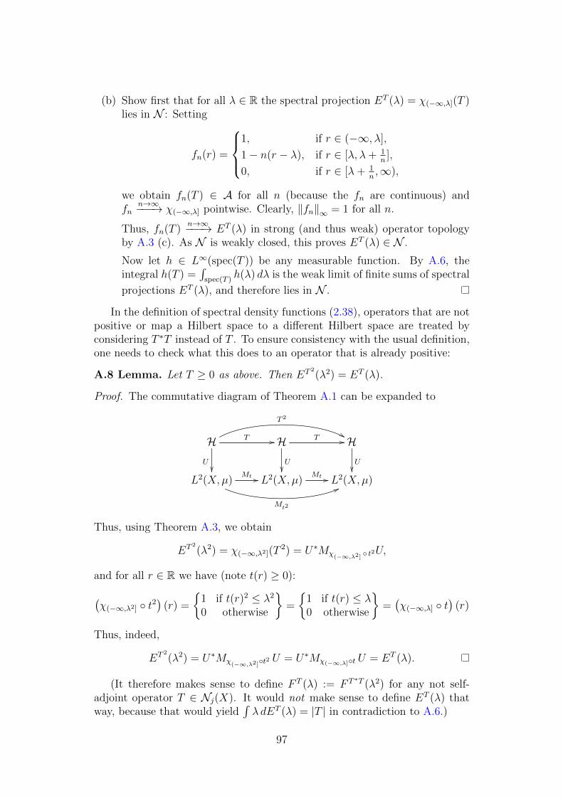
(b) Show first that for all λ ∈ R the spectral projection ET (λ) = χ(−∞,λ](T )lies in N : Setting
fn(r) =
1, if r ∈ (−∞, λ],
1− n(r − λ), if r ∈ [λ, λ+ 1n],
0, if r ∈ [λ+ 1n,∞),
we obtain fn(T ) ∈ A for all n (because the fn are continuous) andfn
n→∞−−−→ χ(−∞,λ] pointwise. Clearly, ‖fn‖∞ = 1 for all n.
Thus, fn(T )n→∞−−−→ ET (λ) in strong (and thus weak) operator topology
by A.3 (c). As N is weakly closed, this proves ET (λ) ∈ N .
Now let h ∈ L∞(spec(T )) be any measurable function. By A.6, theintegral h(T ) =
∫spec(T )
h(λ) dλ is the weak limit of finite sums of spectral
projections ET (λ), and therefore lies in N .
In the definition of spectral density functions (2.38), operators that are notpositive or map a Hilbert space to a different Hilbert space are treated byconsidering T ∗T instead of T . To ensure consistency with the usual definition,one needs to check what this does to an operator that is already positive:
A.8 Lemma. Let T ≥ 0 as above. Then ET 2(λ2) = ET (λ).
Proof. The commutative diagram of Theorem A.1 can be expanded to
H T //
U
T 2
&&H T //
U
HU
L2(X,µ)Mt //
Mt2
66L2(X,µ)
Mt // L2(X,µ)
Thus, using Theorem A.3, we obtain
ET 2
(λ2) = χ(−∞,λ2](T2) = U∗Mχ(−∞,λ2] t2U,
and for all r ∈ R we have (note t(r) ≥ 0):(χ(−∞,λ2] t2
)(r) =
1 if t(r)2 ≤ λ2
0 otherwise
=
1 if t(r) ≤ λ0 otherwise
=(χ(−∞,λ] t
)(r)
Thus, indeed,
ET 2
(λ2) = U∗Mχ(−∞,λ2]t2 U = U∗Mχ(−∞,λ]t U = ET (λ).
(It therefore makes sense to define F T (λ) := F T ∗T (λ2) for any not self-adjoint operator T ∈ Nj(X). It would not make sense to define ET (λ) thatway, because that would yield
∫λ dET (λ) = |T | in contradiction to A.6.)
97
Finally, let us note the following “interpretation” of the spectral projec-tions: Simply speaking, the image of ET (λ) is a maximal subspace on whichT is bounded by λ.
A.9 Lemma. Assume the conditions and notation of Theorem A.1, and letv ∈ H be nonzero. Then
ET (λ) v = v =⇒ ‖Tv‖ ≤ λ ‖v‖ ,ET (λ) v = 0 =⇒ ‖Tv‖ > λ ‖v‖ .
Proof. Either see [Luc02], Lemma 2.2, p. 73, or consider the following:Using Theorems A.1, A.3 and A.6, we have the commutative diagram
H ET (λ) //
U
HU
L2(X,µ)Mχ // L2(X,µ)
where χ = χ(−∞,λ] t ∈ L∞(X) is the characteristic function of the setx ∈ X | |t(x)| ≤ λ. (Thus, 1 − χ is the characteristic function of the setx ∈ X | |t(x)| > λ.) Fix v ∈ H and let Uv be given by the function f ∈L2(X,µ). Then we have:
‖Tv‖2H = ‖UTv‖2
2 =
∫X
|t · f |2 dµ
=
∫X
|t · f |2 · χdµ+
∫X
|t · f |2 · (1− χ) dµ
If ET (λ)v = v, then χ · f = f (and thus (1− χ) · f = 0), so
‖Tv‖2H =
∫X
|t · f |2 · χdµ =
∫x | |t(x)|≤λ
|t · f |2 dµ
≤ λ2
∫X
|f |2 dµ = λ2 ‖Uv‖22 = λ2 ‖v‖2
H .
Finally, if ET (λ)v = 0, then χ · f = 0, so
‖Tv‖2H =
∫X
|t · f |2 · (1− χ) dµ =
∫x | |t(x)|>λ
|t · f |2 dµ
> λ2
∫X
|f |2 dµ = λ2 ‖Uv‖22 = λ2 ‖v‖2
H .
(Of course, the “greater than” requires that the integral is nonzero; that is thecase since ‖f‖2 = ‖v‖H > 0.)
98
References
[Alo86] N. Alon. Eigenvalues and expanders. Combinatorica, 6:83–96, 1986.
[Ati76] Michael F. Atiyah. Elliptic operators, discrete groups and von Neu-mann algebras. Asterisque, 32-33:43–72, 1976.
[CGI09] Fabio Cipriani, Daniele Guido, and Tommaso Isola. A C∗-algebra ofgeometric operators on self-similar CW-complexes. Novikov-Shubinand L2-Betti numbers. J. Funct. Anal., 256(3):603–634, 2009.
[DLM+03] Jozef Dodziuk, Peter Linnell, Varghese Mathai, Thomas Schick,and Stuart Yates. Approximating L2-invariants and the Atiyah con-jecture. Commun. Pure Appl. Math., 56(7):839–873, 2003.
[DM98] Jozef Dodziuk and Varghese Mathai. Approximating L2 invariantsof amenable covering spaces: A combinatorial approach. J. Funct.Anal., 154(2):359–378, art. no. fu973205, 1998.
[Ele06] Gabor Elek. L2-spectral invariants and quasi-crystal graphs. arXivMathematics e-prints, page math/0607198, Jul 2006.
[Ele08] Gabor Elek. L2-spectral invariants and convergent sequences of finitegraphs. J. Funct. Anal., 254(10):2667–2689, 2008.
[Els11] Jurgen Elstrodt. Maß- und Integrationstheorie. Berlin - Heidelberg:Springer-Verlag, 2011.
[FK52] Bent Fuglede and Richard V. Kadison. Determinant theory in finitefactors. Ann. Math. (2), 55:520–530, 1952.
[GH91] C.P.M. Geerse and A. Hof. Lattice Gas Models on Self-Similar Ape-riodic Tilings. Rev. Math. Phys., 03:163–221, 1991.
[Gro81] Mikhael Gromov. Groups of polynomial growth and expanding maps(with an appendix by Jacques Tits). Publications Mathematiques del’IHES, 53:53–78, 1981.
[Hat02] Allen Hatcher. Algebraic topology. Cambridge: Cambridge UniversityPress, 2002.
[Heu09] Harro Heuser. Lehrbuch der Analysis. Teil 1. Wiesbaden:Vieweg+Teubner, 17th revised ed. edition, 2009.
[Hew60] Edwin Hewitt. Integration by parts for Stieltjes integrals. Am. Math.Mon., 67:419–423, 1960.
[Kam17] Holger Kammeyer. Approximating Novikov-Shubin numbers of vir-tually cyclic coverings. Groups Geom. Dyn., 11(4):1231–1251, 2017.
99
[Kam19] Holger Kammeyer. Introduction to `2-invariants., volume 2247.Cham: Springer, 2019.
[Kel95] Johannes Kellendonk. Noncommutative geometry of tilings and gaplabelling. Rev. Math. Phys., 7(7):1133–1180, 1995.
[Lot92] John Lott. Heat kernels on covering spaces and topological invariants.J. Differ. Geom., 35(2):471–510, 1992.
[Luc02] Wolfgang Luck. L2-Invariants: Theory and Applications to Geometryand K-Theory. Berlin - Heidelberg - New York: Springer-Verlag,2002.
[Luc05] Wolfgang Luck. Algebraische Topologie. Homologie und Mannig-faltigkeiten. Wiesbaden: Vieweg, 2005.
[Luc16] Wolfgang Luck. Approximating L2-invariants by their classical coun-terparts. EMS Surv. Math. Sci., 3(2):269–344, 2016.
[NS86] S. P. Novikov and M. A. Shubin. Morse inequalities and von Neu-mann II1-factors. Sov. Math., Dokl., 34:79–82, 1986.
[RS72] Michael Reed and Barry Simon. Methods of modern mathematicalphysics. 1: Functional analysis. 1972.
[Suc16] Engelbert Suchla. Traces for Geometric Operators on Self-SimilarCW-Complexes and Generalizations. Master thesis, Georg-August-Universitat Gottingen, 2016.
[Var87] N. Th. Varopoulos. Random walks and Brownian motion on mani-folds. Harmonic analysis, symmetric spaces and probability theory,Cortona/Italy 1984, Symp. Math. 29, 97-109 (1987)., 1987.
[von50] John von Neumann. Functional operators. Vol. II. The geometry oforthogonal spaces., volume 22. Princeton University Press, Princeton,NJ, 1950.
[Woe00] Wolfgang Woess. Random walks on infinite graphs and groups., vol-ume 138. Cambridge: Cambridge University Press, 2000.
100


![arXiv:0708.0798v2 [math.RT] 11 Oct 2008 › pdf › 0708.0798.pdf · 2018-11-23 · arXiv:0708.0798v2 [math.RT] 11 Oct 2008 CLUSTER COMPLEXES VIA SEMI-INVARIANTS KIYOSHI IGUSA, KENT](https://img.pdfslide.us/doc/110x75/5f0f13437e708231d4425dfe/arxiv07080798v2-mathrt-11-oct-2008-a-pdf-a-07080798pdf-2018-11-23.jpg)
![Coreduction Homology Algorithm for Regular CW-Complexesdlotko/cwcored.pdfframework, i.e., the theory of S-complexes which was introduced in [19]asarefor-mulation of the concept of](https://img.pdfslide.us/doc/110x75/6116068fb16e8865052cd83f/coreduction-homology-algorithm-for-regular-cw-complexes-dlotko-framework-ie.jpg)