Embed Size (px)
Citation preview
CSE373, Winter 2020L18: Disjoint Sets
Disjoint SetsCSE 373 Winter 2020
Instructor: Hannah C. Tang
Teaching Assistants:
Aaron Johnston Ethan Knutson Nathan Lipiarski
Amanda Park Farrell Fileas Sam Long
Anish Velagapudi Howard Xiao Yifan Bai
Brian Chan Jade Watkins Yuma Tou
Elena Spasova Lea Quan
CSE373, Winter 2020L18: Disjoint Sets
Announcements
❖ HW7 released; due Fri, Feb 28
▪ HW7 exercises a different set of skills: reading/understanding a large codebase and figuring out where to plug in
▪ Read the spec carefully; HW7 substantially longer than last quarter’s because we added a ton of hints
3

CSE373, Winter 2020L18: Disjoint Sets
Feedback from Reading Quiz
❖ When do we use Disjoint Sets?
❖ Can we make union() constant time?
❖ How did you choose the values for the ids?
4
CSE373, Winter 2020L18: Disjoint Sets
Lecture Outline
❖ Disjoint Set ADT
❖ QuickFind Data Structure
❖ QuickUnion Data Structure
❖ WeightedQuickUnion Data Structure
▪ Path Compression
5
CSE373, Winter 2020L18: Disjoint Sets
Disjoint Sets ADT
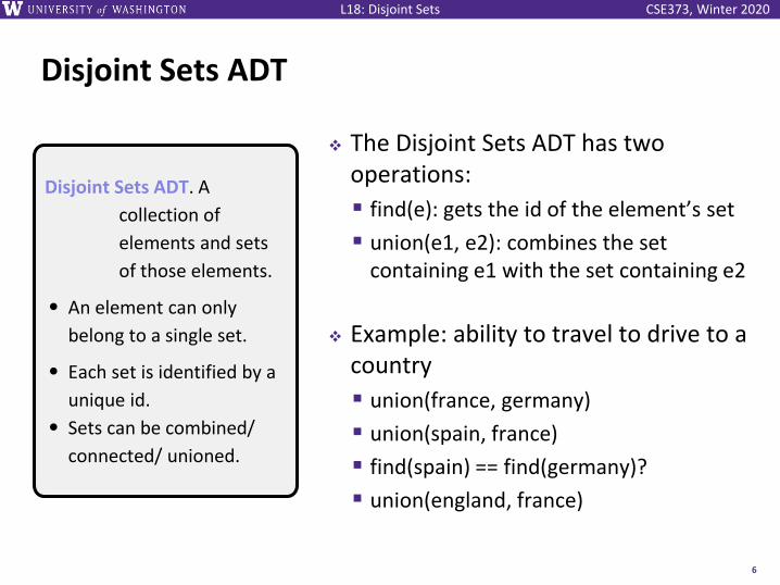
❖ The Disjoint Sets ADT has two operations:
▪ find(e): gets the id of the element’s set
▪ union(e1, e2): combines the set containing e1 with the set containing e2
❖ Example: ability to travel to drive to a country
▪ union(france, germany)
▪ union(spain, france)
▪ find(spain) == find(germany)?
▪ union(england, france)
6
Disjoint Sets ADT. A
collection of
elements and sets
of those elements.
• An element can only
belong to a single set.
• Each set is identified by a
unique id.
• Sets can be combined/
connected/ unioned.
CSE373, Winter 2020L18: Disjoint Sets
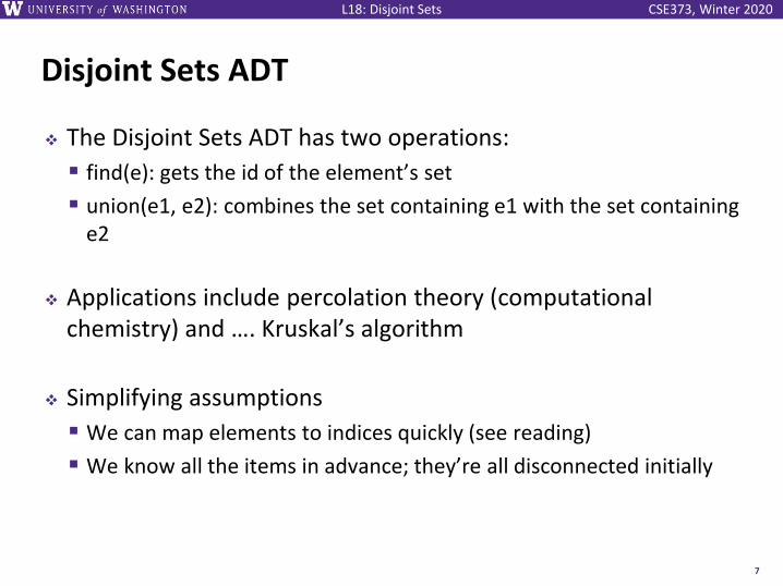
Disjoint Sets ADT
❖ The Disjoint Sets ADT has two operations:
▪ find(e): gets the id of the element’s set
▪ union(e1, e2): combines the set containing e1 with the set containing e2
❖ Applications include percolation theory (computational chemistry) and …. Kruskal’s algorithm
❖ Simplifying assumptions
▪ We can map elements to indices quickly (see reading)
▪ We know all the items in advance; they’re all disconnected initially
7

CSE373, Winter 2020L18: Disjoint Sets
An Observation …
❖ Today’s lecture on the data structures which implement the Disjoint Sets ADT is an interesting case study in data structure design and iterative design improvements
▪ Dust off your metacognitive skills and pay attention to what stays the same and what changes between our 3 options
8
CSE373, Winter 2020L18: Disjoint Sets
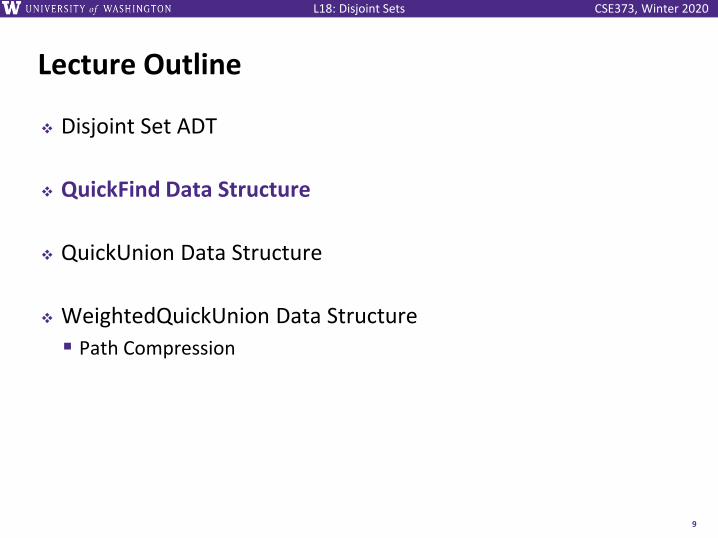
Lecture Outline
❖ Disjoint Set ADT
❖ QuickFind Data Structure
❖ QuickUnion Data Structure
❖ WeightedQuickUnion Data Structure
▪ Path Compression
9
CSE373, Winter 2020L18: Disjoint Sets
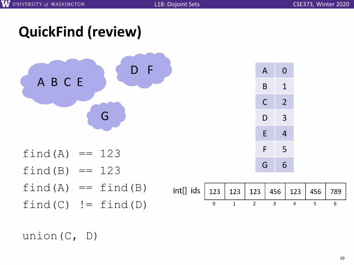
QuickFind (review)
find(A) == 123
find(B) == 123
find(A) == find(B)
find(C) != find(D)
union(C, D)
10
A 0
B 1
C 2
D 3
E 4
F 5
G 6
A B C E D F
G
CSE373, Winter 2020L18: Disjoint Sets
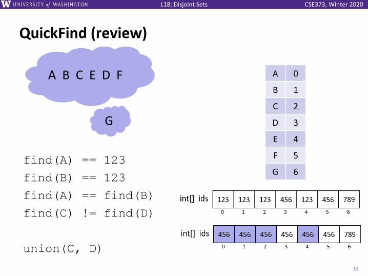
QuickFind (review)
find(A) == 123
find(B) == 123
find(A) == find(B)
find(C) != find(D)
union(C, D)
11
A 0
B 1
C 2
D 3
E 4
F 5
G 6
A B C E D F
G
CSE373, Winter 2020L18: Disjoint Sets
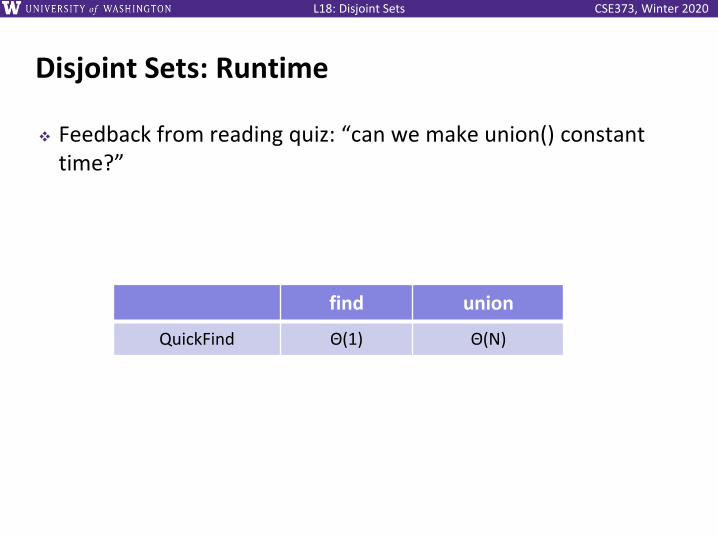
Disjoint Sets: Runtime
❖ Feedback from reading quiz: “can we make union() constant time?”
find union
QuickFind Θ(1) Θ(N)
CSE373, Winter 2020L18: Disjoint Sets
Lecture Outline
❖ Disjoint Set ADT
❖ QuickFind Data Structure
❖ QuickUnion Data Structure
❖ WeightedQuickUnion Data Structure
▪ Path Compression
13
CSE373, Winter 2020L18: Disjoint Sets
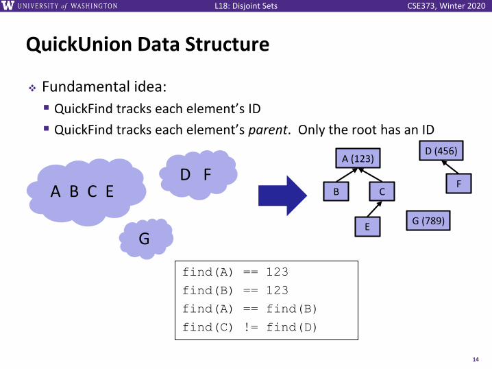
QuickUnion Data Structure
❖ Fundamental idea:
▪ QuickFind tracks each element’s ID
▪ QuickFind tracks each element’s parent. Only the root has an ID
14
A B C E D F
G
D (456)
F
G (789)
A (123)
CB
E
find(A) == 123
find(B) == 123
find(A) == find(B)
find(C) != find(D)
CSE373, Winter 2020L18: Disjoint Sets
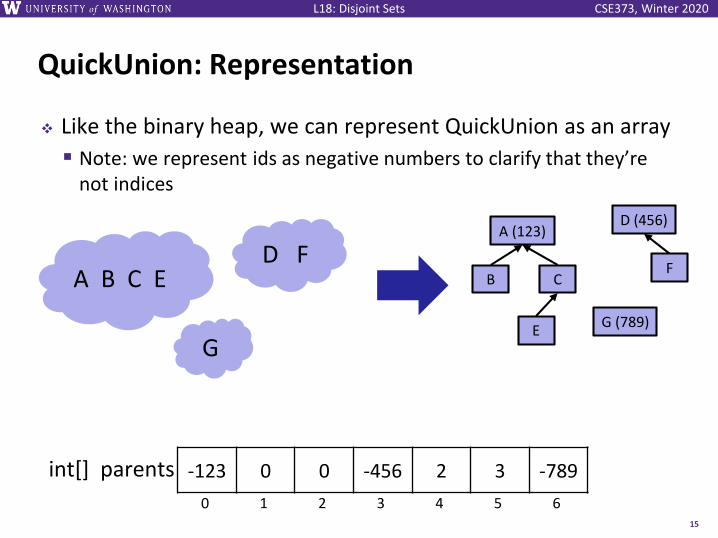
QuickUnion: Representation
❖ Like the binary heap, we can represent QuickUnion as an array
▪ Note: we represent ids as negative numbers to clarify that they’re not indices
15
A B C E D F
G
D (456)
F
G (789)
A (123)
CB
E
-123 0 0 -456 2 3 -789int[] parents
0 1 2 3 4 5 6
CSE373, Winter 2020L18: Disjoint Sets
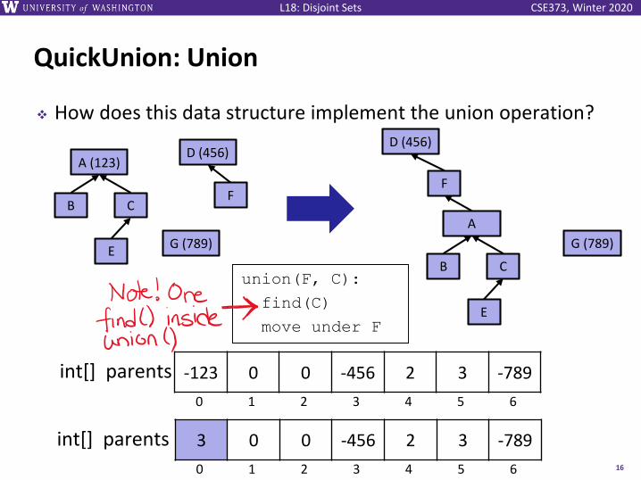
QuickUnion: Union
❖ How does this data structure implement the union operation?
16
G (789)
union(F, C):
find(C)
move under F
D (456)
F
A
CB
E
3 0 0 -456 2 3 -789int[] parents
0 1 2 3 4 5 6
-123 0 0 -456 2 3 -789int[] parents
0 1 2 3 4 5 6
D (456)
F
G (789)
A (123)
CB
E
CSE373, Winter 2020L18: Disjoint Sets
pollev.com/uwcse373
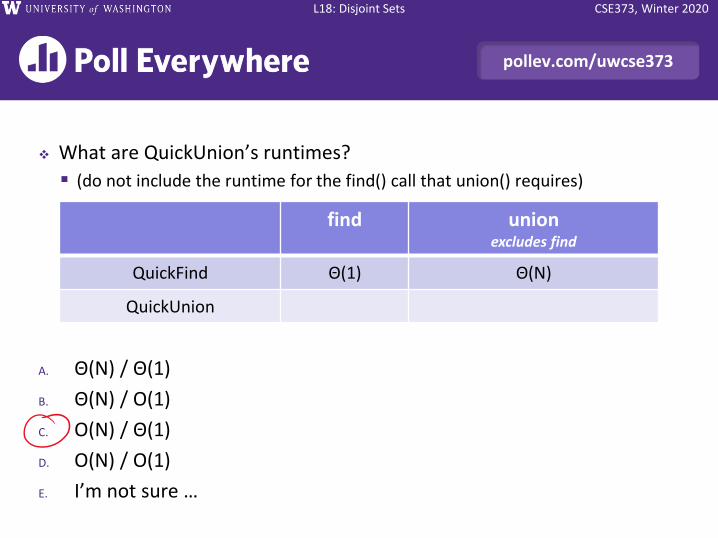
❖ What are QuickUnion’s runtimes?
▪ (do not include the runtime for the find() call that union() requires)
A. Θ(N) / Θ(1)
B. Θ(N) / O(1)
C. O(N) / Θ(1)
D. O(N) / O(1)
E. I’m not sure …
find unionexcludes find
QuickFind Θ(1) Θ(N)
QuickUnion
CSE373, Winter 2020L18: Disjoint Sets
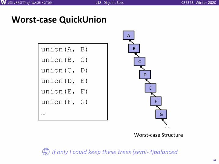
Worst-case QuickUnion
union(A, B)
union(B, C)
union(C, D)
union(D, E)
union(E, F)
union(F, G)
…
18
B
Worst-case Structure
A
C
D
E
F
G
…
🤔 If only I could keep these trees (semi-?)balanced
CSE373, Winter 2020L18: Disjoint Sets
Lecture Outline
❖ Disjoint Set ADT
❖ QuickFind Data Structure
❖ QuickUnion Data Structure
❖ WeightedQuickUnion Data Structure
▪ Path Compression
19

CSE373, Winter 2020L18: Disjoint Sets
WeightedQuickUnion
20
C
A
B
union(A, B)
union(B, C)
union(C, D)
union(D, E)
union(E, F)
union(F, G)
…
D
E
F
G
?
❖ QuickUnion always picked the same argument (the second argument) to become the child in the unioned structure
❖ QuickUnion only found the root of the second argument
❖ Instead, let’s:
▪ Pick the smaller tree to be the new child
▪ Add the new child to the root
CSE373, Winter 2020L18: Disjoint Sets
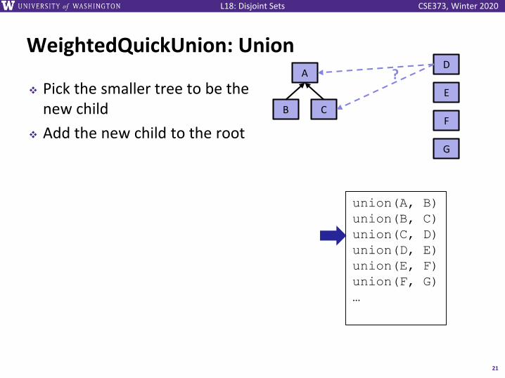
WeightedQuickUnion: Union
21
C
A
B
union(A, B)
union(B, C)
union(C, D)
union(D, E)
union(E, F)
union(F, G)
…
❖ Pick the smaller tree to be the new child
❖ Add the new child to the root
D
E
F
G
?
CSE373, Winter 2020L18: Disjoint Sets
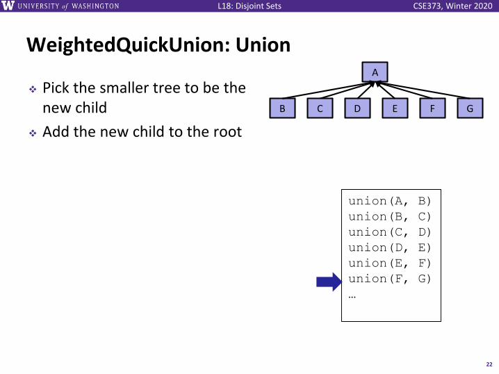
WeightedQuickUnion: Union
22
C
A
B D E F G
union(A, B)
union(B, C)
union(C, D)
union(D, E)
union(E, F)
union(F, G)
…
❖ Pick the smaller tree to be the new child
❖ Add the new child to the root
CSE373, Winter 2020L18: Disjoint Sets
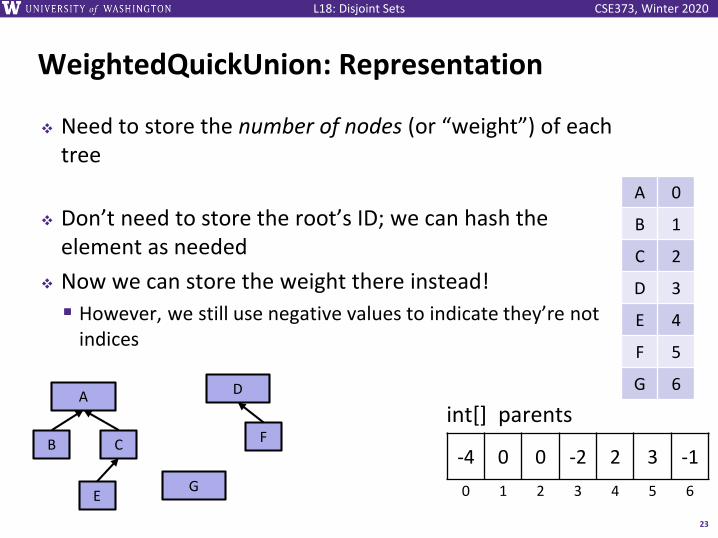
WeightedQuickUnion: Representation
❖ Need to store the number of nodes (or “weight”) of each tree
❖ Don’t need to store the root’s ID; we can hash the element as needed
❖ Now we can store the weight there instead!
▪ However, we still use negative values to indicate they’re not indices
23
A 0
B 1
C 2
D 3
E 4
F 5
G 6
-4 0 0 -2 2 3 -1
0 1 2 3 4 5 6
D
F
G
A
CB
E
int[] parents
CSE373, Winter 2020L18: Disjoint Sets
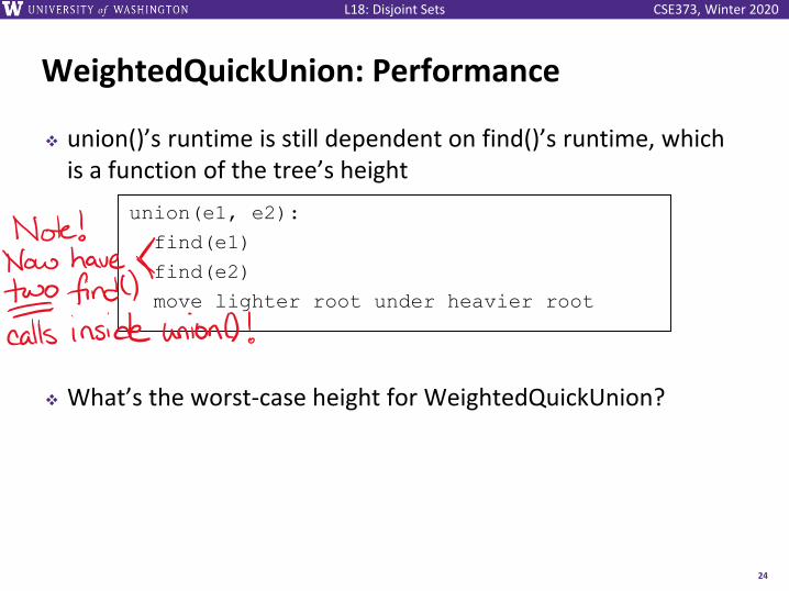
WeightedQuickUnion: Performance
❖ union()’s runtime is still dependent on find()’s runtime, which is a function of the tree’s height
❖ What’s the worst-case height for WeightedQuickUnion?
24
union(e1, e2):
find(e1)
find(e2)
move lighter root under heavier root
CSE373, Winter 2020L18: Disjoint Sets
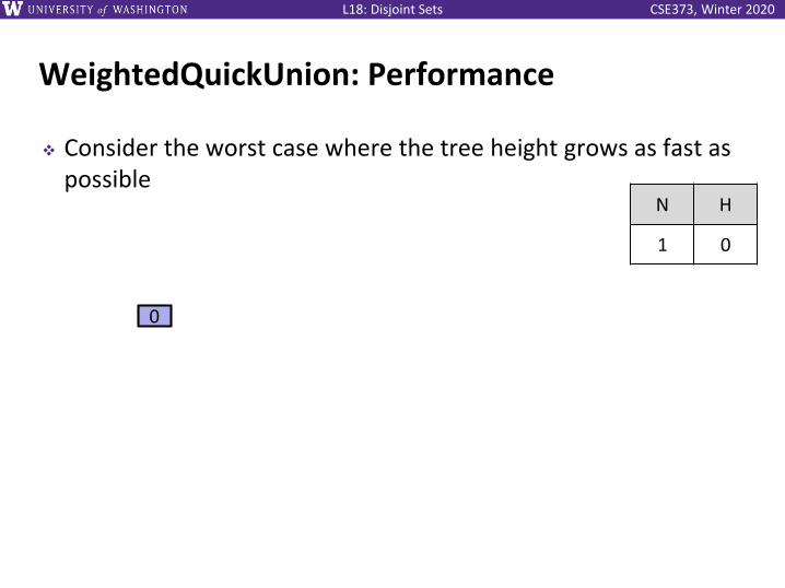
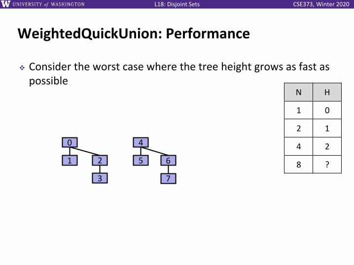
WeightedQuickUnion: Performance
❖ Consider the worst case where the tree height grows as fast as possible
0
N H
1 0
CSE373, Winter 2020L18: Disjoint Sets
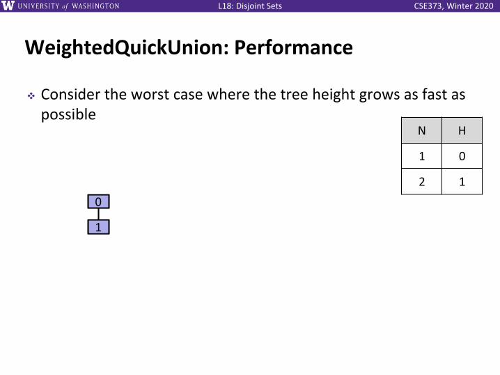
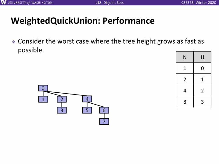
WeightedQuickUnion: Performance
❖ Consider the worst case where the tree height grows as fast as possible
0
1
N H
1 0
2 1
CSE373, Winter 2020L18: Disjoint Sets
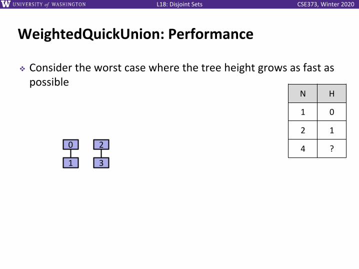
WeightedQuickUnion: Performance
❖ Consider the worst case where the tree height grows as fast as possible
0
1
2
3
N H
1 0
2 1
4 ?
CSE373, Winter 2020L18: Disjoint Sets
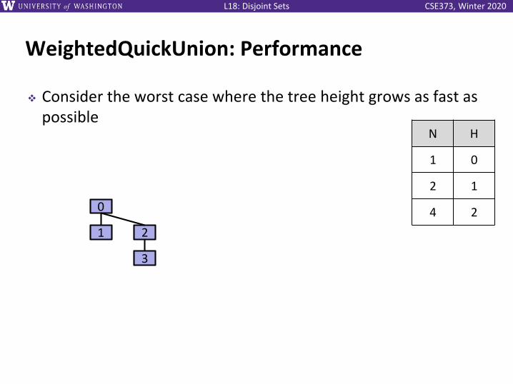
WeightedQuickUnion: Performance
❖ Consider the worst case where the tree height grows as fast as possible
0
1 2
3
N H
1 0
2 1
4 2
CSE373, Winter 2020L18: Disjoint Sets
WeightedQuickUnion: Performance
❖ Consider the worst case where the tree height grows as fast as possible
0
1 2
3
4
5 6
7
N H
1 0
2 1
4 2
8 ?
CSE373, Winter 2020L18: Disjoint Sets
WeightedQuickUnion: Performance
❖ Consider the worst case where the tree height grows as fast as possible
0
1 2
3
N H
1 0
2 1
4 2
8 34
5 6
7
CSE373, Winter 2020L18: Disjoint Sets
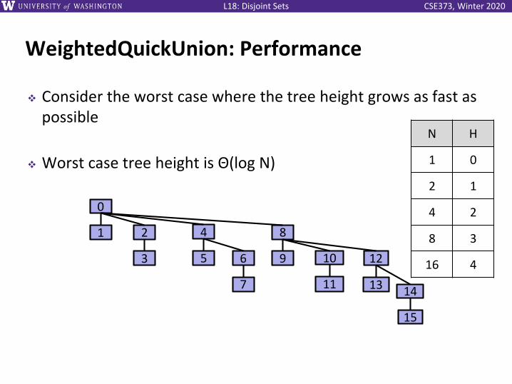
WeightedQuickUnion: Performance
❖ Consider the worst case where the tree height grows as fast as possible
❖ Worst case tree height is Θ(log N)
0
1 2
3
N H
1 0
2 1
4 2
8 3
16 4
4
5 6
7
8
9 10
11
12
13 14
15
CSE373, Winter 2020L18: Disjoint Sets
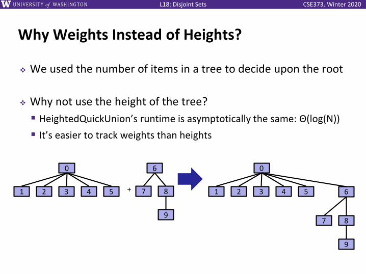
Why Weights Instead of Heights?
❖ We used the number of items in a tree to decide upon the root
❖ Why not use the height of the tree?
▪ HeightedQuickUnion’s runtime is asymptotically the same: Θ(log(N))
▪ It’s easier to track weights than heights
1 2
0
4
6
53 8
9
7+ 1 2
0
4 653
8
9
7
CSE373, Winter 2020L18: Disjoint Sets
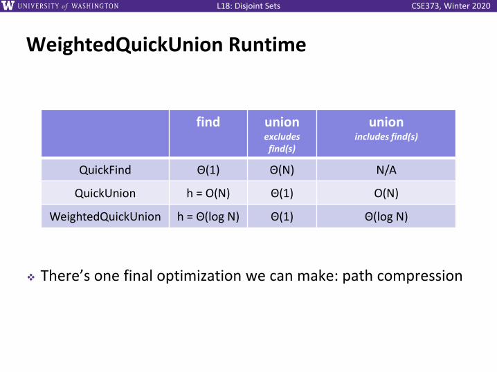
WeightedQuickUnion Runtime
❖ There’s one final optimization we can make: path compression
find unionexcludes find(s)
unionincludes find(s)
QuickFind Θ(1) Θ(N) N/A
QuickUnion h = O(N) Θ(1) O(N)
WeightedQuickUnion h = Θ(log N) Θ(1) Θ(log N)
CSE373, Winter 2020L18: Disjoint Sets
Lecture Outline
❖ Disjoint Set ADT
❖ QuickFind Data Structure
❖ QuickUnion Data Structure
❖ WeightedQuickUnion Data Structure
▪ Path Compression
34
CSE373, Winter 2020L18: Disjoint Sets
Modifying Data Structures To Preserve Invariants
❖ Thus far, the modifications we’ve studied are designed to preserve invariants (aka “repair the data structure”)
▪ Tree rotations: preserve LLRB tree invariants (eg, a right-leaning red edge)
▪ Promoting keys / splitting leaves: preserve B-tree invariants (eg, L+1 keys stored in a leaf node)
❖ Notably, the modifications don’t improve runtime between identical method calls
▪ If bst.find(x) takes 2 µs, we expect future calls to take ~2 µs
▪ If we call bst.find(x) M times, the total runtime should be 2*M µs
35
CSE373, Winter 2020L18: Disjoint Sets
Modifying Data Structures for Future Gains
❖ Path compression is entirely different: we are modifying the tree structure to improve future performance
▪ If wquWithPathCompression.find(x) takes 2 µs, we expect future calls to take <2 µs
▪ If we call wquWithPathCompression.find(x) M times, the total runtime should be <2*M µs (and possibly even << 2*M µs)
36
CSE373, Winter 2020L18: Disjoint Sets
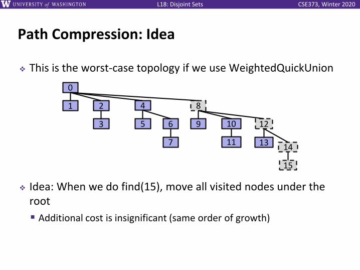
Path Compression: Idea
❖ This is the worst-case topology if we use WeightedQuickUnion
❖ Idea: When we do find(15), move all visited nodes under the root
▪ Additional cost is insignificant (same order of growth)
0
1 2
3
4
5 6
7
8
9 10
11
12
13 14
15
CSE373, Winter 2020L18: Disjoint Sets
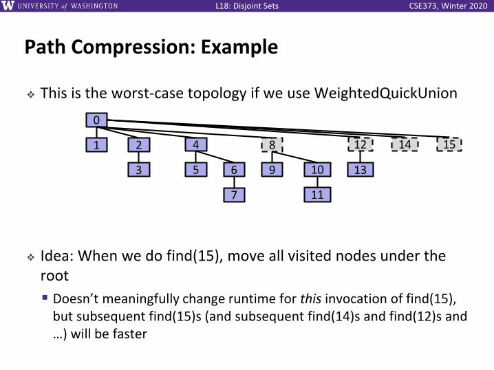
Path Compression: Example
❖ This is the worst-case topology if we use WeightedQuickUnion
❖ Idea: When we do find(15), move all visited nodes under the root
▪ Doesn’t meaningfully change runtime for this invocation of find(15), but subsequent find(15)s (and subsequent find(14)s and find(12)s and …) will be faster
0
1 2
3
4
5 6
7
8
9 10
11
12
13
14 15
CSE373, Winter 2020L18: Disjoint Sets
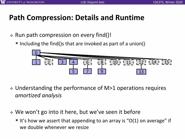
Path Compression: Details and Runtime
❖ Run path compression on every find()!
▪ Including the find()s that are invoked as part of a union()
❖ Understanding the performance of M>1 operations requires amortized analysis
❖ We won’t go into it here, but we’ve seen it before
▪ It’s how we assert that appending to an array is “O(1) on average” if we double whenever we resize
0
1 2 3 4
5
6
7
8
9
10 11 12
13
14 15
CSE373, Winter 2020L18: Disjoint Sets
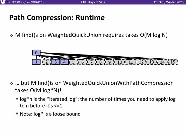
Path Compression: Runtime
❖ M find()s on WeightedQuickUnion requires takes Θ(M log N)
❖ … but M find()s on WeightedQuickUnionWithPathCompression takes O(M log*N)!
▪ log*n is the “iterated log”: the number of times you need to apply log to n before it’s <=1
▪ Note: log* is a loose bound
0
1 2 3 4 5 6 7 8 9 10 11 12 13 14 15
CSE373, Winter 2020L18: Disjoint Sets
Path Compression: Runtime
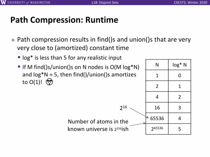
❖ Path compression results in find()s and union()s that are very very close to (amortized) constant time
▪ log* is less than 5 for any realistic input
▪ If M find()s/union()s on N nodes is O(M log*N)and log*N ≈ 5, then find()/union()s amortizesto O(1)! 🤯
N log* N
1 0
2 1
4 2
16 3
65536 4
265536 5
216
Number of atoms in the known universe is 2256ish
CSE373, Winter 2020L18: Disjoint Sets
tl;dr
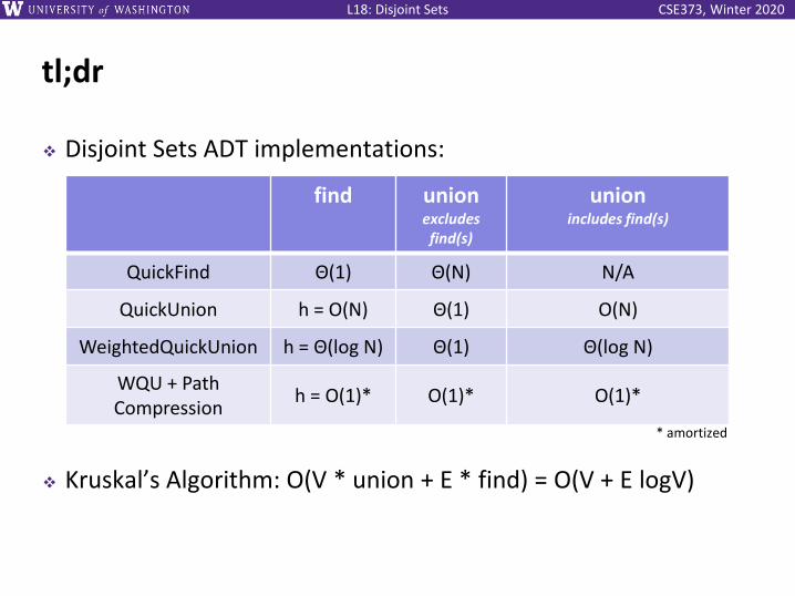
❖ Disjoint Sets ADT implementations:
❖ Kruskal’s Algorithm: O(V * union + E * find) = O(V + E logV)
find unionexcludes find(s)
unionincludes find(s)
QuickFind Θ(1) Θ(N) N/A
QuickUnion h = O(N) Θ(1) O(N)
WeightedQuickUnion h = Θ(log N) Θ(1) Θ(log N)
WQU + Path Compression
h = O(1)* O(1)* O(1)*
* amortized