Embed Size (px)
Citation preview

L11: Risk Sharing and Asset Pricing 1
Lecture 11: Risk Sharing and Asset Pricing
• The following topics will be covered:• Pareto Efficient Risk Allocation (assuming we have a social
planner)– Defining Pareto Improvement and Pareto Efficient
– Mutuality Principle
– Optimal Risk Sharing
• Asset Pricing (assuming complete market)– First Theorem of Welfare Economics
– Equity Premium
– CAPM
– Interest rate determination
Materials from Chapter 10 and 11 of EGS
L11: Risk Sharing and Asset Pricing 2
Pareto Efficient
Given a set of alternative allocations of say goods or income for a set of individuals, a movement from one allocation to another that can make at least one individual better off, without making any other individual worse off, is called a Pareto improvement. An allocation is Pareto efficient or Pareto optimal when no further Pareto improvements can be made. This term is named after Vilfredo Pareto, an Italian economist who used the concept in his studies of economic efficiency and income distribution.
L11: Risk Sharing and Asset Pricing 3
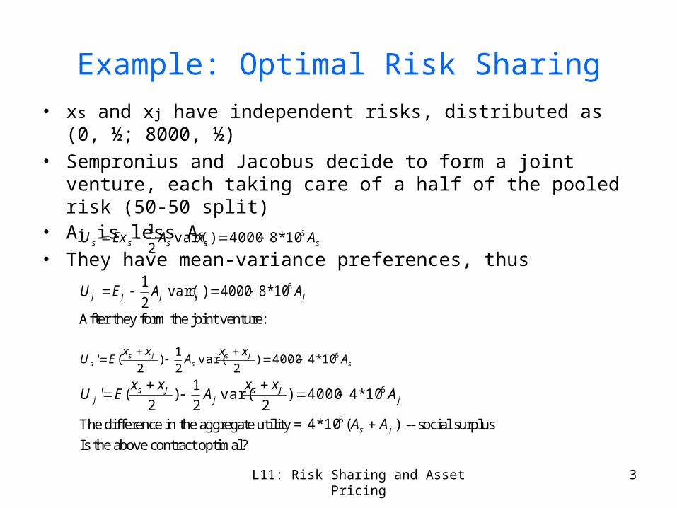
Example: Optimal Risk Sharing
• xs and xj have independent risks, distributed as (0, ½; 8000, ½)
• Sempronius and Jacobus decide to form a joint venture, each taking care of a half of the pooled risk (50-50 split)
• Aj is less As
• They have mean-variance preferences, thussssss AxAExU 610*84000)var(
2
1
JJJJJ AcAEU 610*84000)var(2
1
After they form the joint venture:
sJs
sJs
s Axx
Axx
EU 610*44000)2
var(2
1)
2('
jJs
jJs
j Axx
Axx
EU 610*44000)2
var(2
1)
2('
The difference in the aggregate utility = )(10*4 6js AA -- social surplus
Is the above contract optimal?
L11: Risk Sharing and Asset Pricing 4
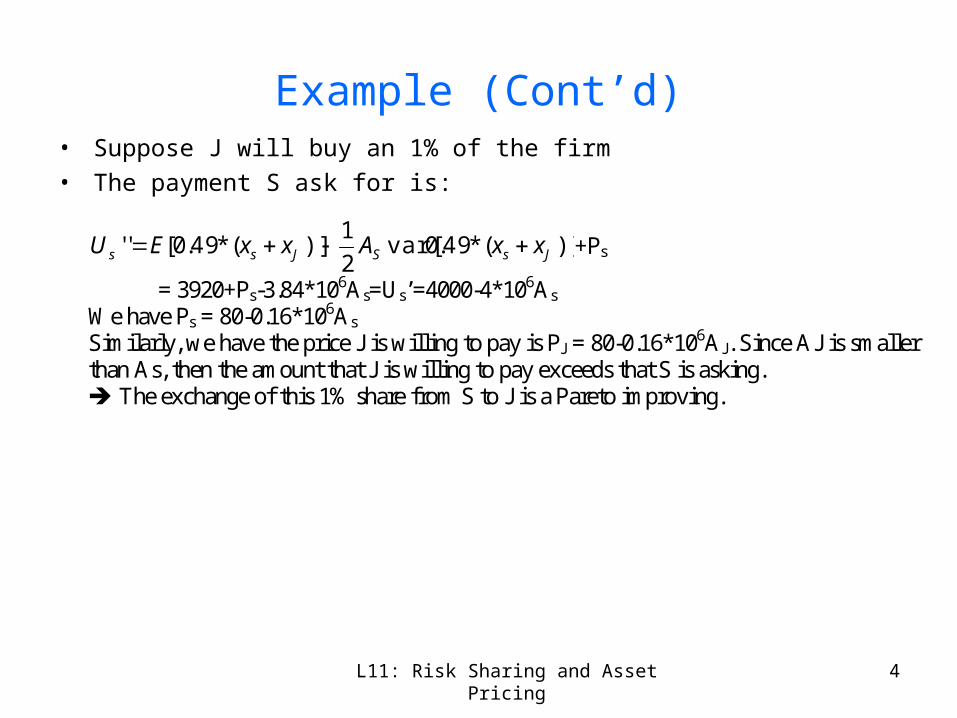
Example (Cont’d)• Suppose J will buy an 1% of the firm
• The payment S ask for is:
)](*49.0var[2
1)](*49.0['' JsSJss xxAxxEU +Ps
= 3920+Ps-3.84*106As=Us’=4000-4*106As
We have Ps = 80-0.16*106As Similarly, we have the price J is willing to pay is PJ = 80-0.16*106AJ. Since AJ is smaller than As, then the amount that J is willing to pay exceeds that S is asking. The exchange of this 1% share from S to J is a Pareto improving.
L11: Risk Sharing and Asset Pricing 5
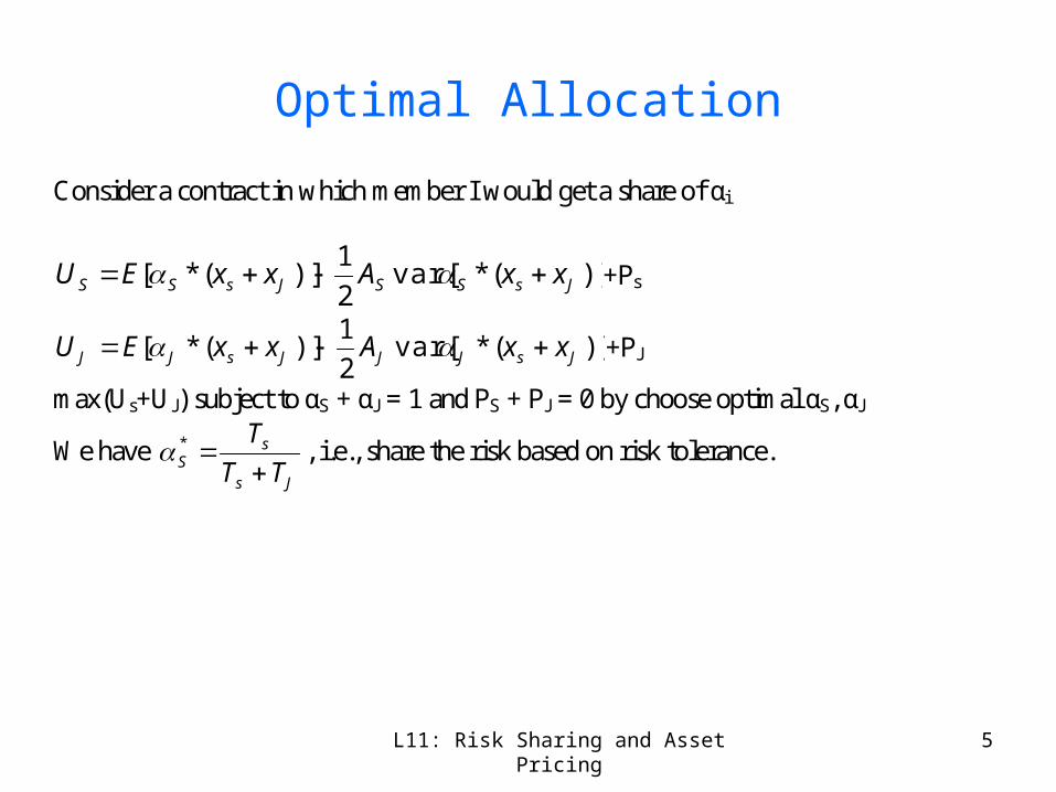
Optimal Allocation
Consider a contract in which member I would get a share of αi
)](*var[2
1)](*[ JsSSJsSS xxAxxEU +Ps
)](*var[2
1)](*[ JsJJJsJJ xxAxxEU +PJ
max(Us+UJ) subject to αS + αJ = 1 and PS + PJ = 0 by choose optimal αS, αJ
We have Js
sS TT
T
* , i.e., share the risk based on risk tolerance.
L11: Risk Sharing and Asset Pricing 6
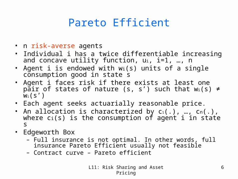
Pareto Efficient
• n risk-averse agents• Individual i has a twice differentiable increasing and concave utility
function, ui, i=1, …, n• Agent i is endowed with wi(s) units of a single consumption good in state s• Agent i faces risk if there exists at least one pair of states of nature (s, s’)
such that wi(s) ≠ wi(s’)• Each agent seeks actuarially reasonable price.• An allocation is characterized by c1(.), …, cn(.), where ci(s) is the
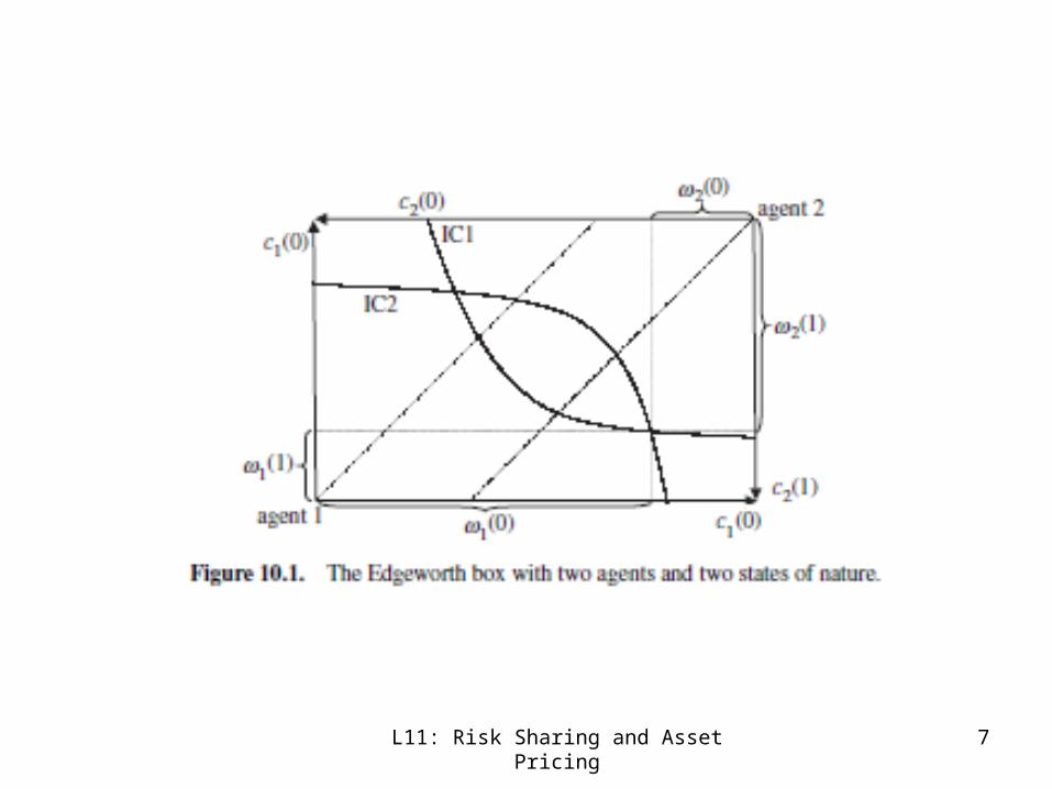
consumption of agent i in state s• Edgeworth Box
– Full insurance is not optimal. In other words, full insurance Pareto Efficient usually not feasible
– Contract curve – Pareto efficient
L11: Risk Sharing and Asset Pricing 7
L11: Risk Sharing and Asset Pricing 8
Characterization of Pareto Efficient Allocation
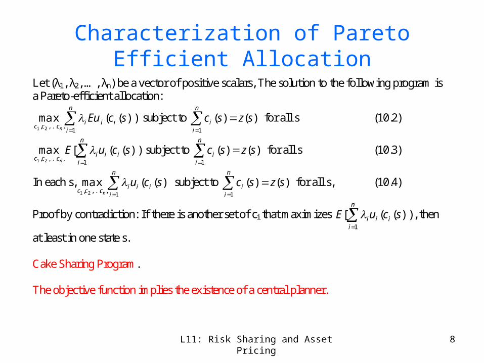
Let (λ1, λ2, …, λn) be a vector of positive scalars, The solution to the following program is a Pareto-efficient allocation:
n
iiii
cccscEu
n 1,...,,
))]((max21
subject to
n
ii szsc
1
),()( for all s (10.2)
n
iiii
cccscuE
n 1,...,,
))](([max21
subject to
n
ii szsc
1
),()( for all s (10.3)
In each s,
n
iiii
cccscu
n 1,...,,
))((max21
subject to
n
ii szsc
1
),()( for all s, (10.4)
Proof by contradiction: If there is another set of ci that maximizes
n
iiii scuE
1
))](([ , then
at least in one state s. Cake Sharing Program. The objective function implies the existence of a central planner.
L11: Risk Sharing and Asset Pricing 9
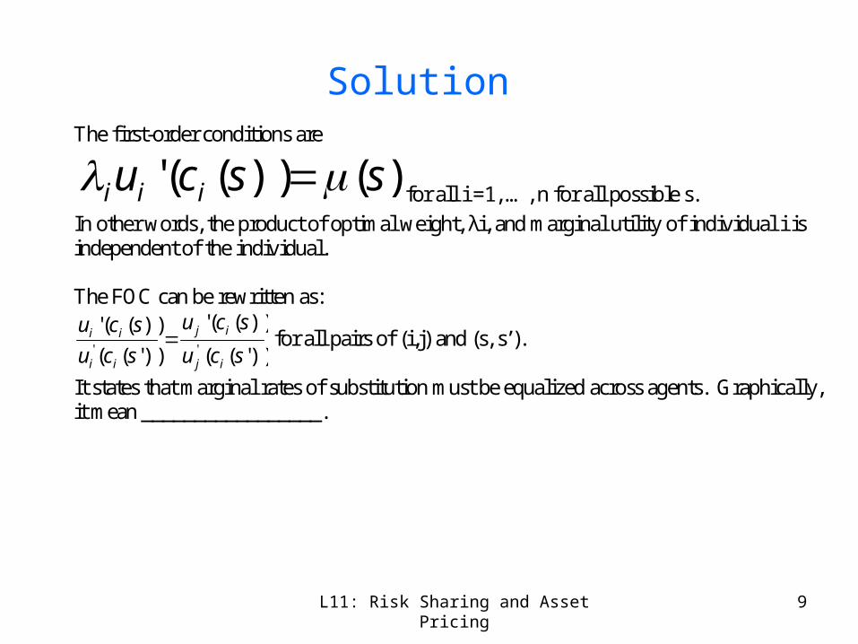
Solution The first-order conditions are
)())((' sscu iii for all i =1, …, n for all possible s.
In other words, the product of optimal weight, λi, and marginal utility of individual i is independent of the individual. The FOC can be rewritten as:
))'((
))(('
))'((
))((''' scu
scu
scu
scu
ij
ij
ii
ii for all pairs of (i,j) and (s, s’).
It states that marginal rates of substitution must be equalized across agents. Graphically, it mean _________________.
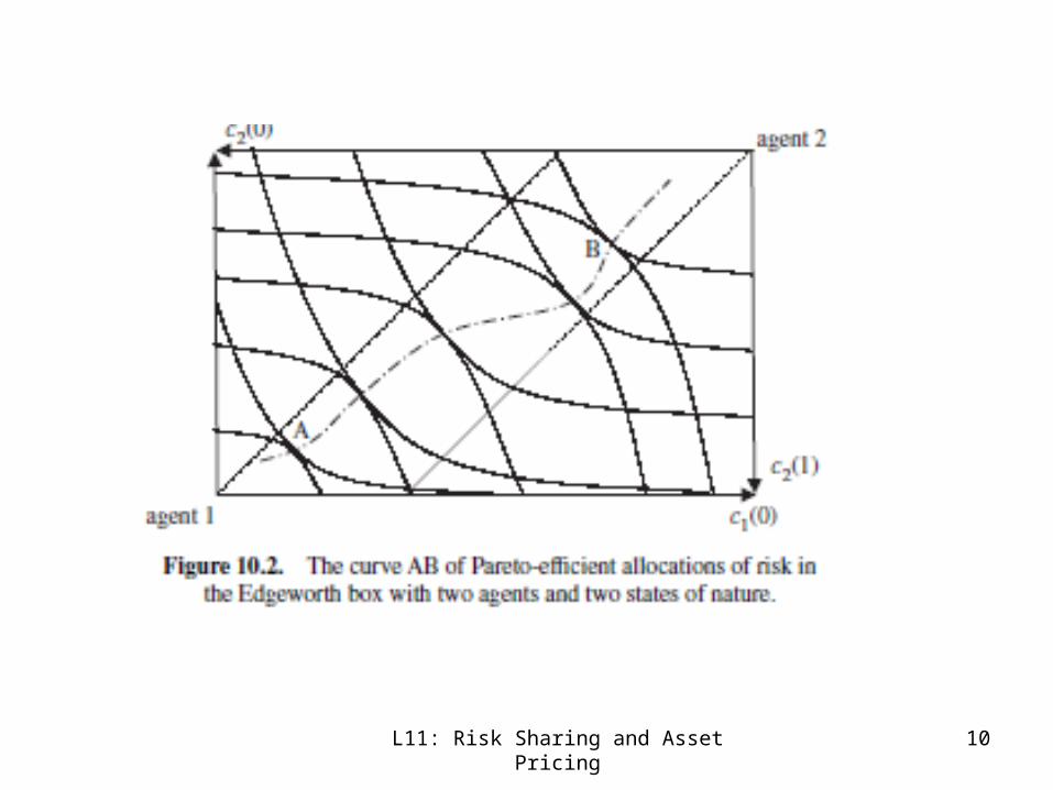
L11: Risk Sharing and Asset Pricing 10
L11: Risk Sharing and Asset Pricing 11
Mutuality Principle
• The Principle: a necessary condition for an allocation of risk to be Pareto efficient is that whenever two states of nature s and s’ have the same level of aggregate wealth, z(s)=z(s’), then for each agent i consumption in state s must be the same as in state s’: ci(s)=ci(s’) for all agent i.
• In other words, z is independent of the state of the nature• There is no aggregate uncertainty in the economy, i.e., no macroeonomic
risk• It is a case of perfect insurance, see figure 10.3 on page 160• However in reality, there are undiversifiable risks -- the economy faces
random events that generate phases of recession or expansion• State price depends on z only.
L11: Risk Sharing and Asset Pricing 12
Sharing of Macroeconomic RiskEach individual selects optimal consumption in state s, thus )())((' sscu iii for all i and s.
Set z(s)=s for all s, we have )())((' zzcu iii
The relationship between ci and z describes agent i’s risk taking incentive: If ci is independent of z, agent I is immune from fluctuations of the aggregate wealth z. If c’(z)=1, agent I bears all of the macroeconomic risk and he insures all other consumers.
The solution is that: for each state z,
N
jjj
iii
zcT
zcTzc
1
'
))((
))(()(
This implies ci’(z)>0. This implies each agent must have more wealth in state s than in state s’ whenever z(s)>z(s’). Graphically, the set of Pareto-efficient solutions is in between the two 45 degree lines.
L11: Risk Sharing and Asset Pricing 13
Examples of Risk Sharing Rule
(1) Risk neutral agent i=1: T1(c) ∞. I.e., c1’(z)=1 and ci’(z)=0 if i not equal to 1. Agent 1 will bear all the risks.
(2) All individuals have constant degree of risk tolerance (CARA)
(3) HARA utility: Ti(c)=ti+αc
See figure 10.4
Ti(c)=ti
It follows that zt
tczc
j j
iii
0)(
zt
zctzc it
i
)()(' . Solving this differential equation, we have:
zt
ctczc it
ii0
0)(
, indicating a linear sharing rule. Kind similar to the illustrated
example.
L11: Risk Sharing and Asset Pricing 14
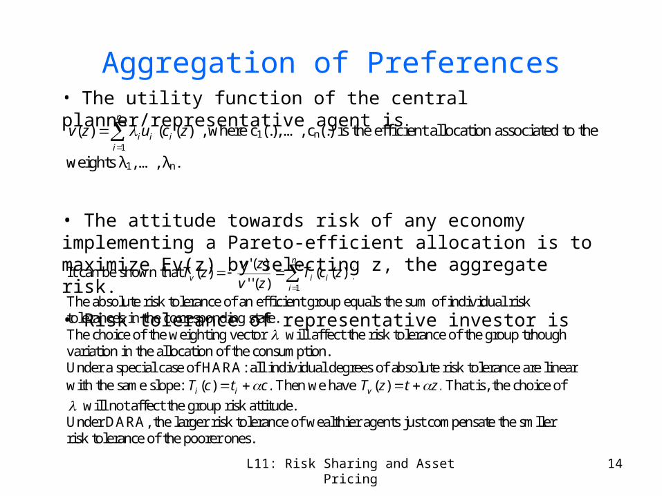
Aggregation of Preferences
• The utility function of the central planner/representative agent is
• The attitude towards risk of any economy implementing a Pareto-efficient allocation is to maximize Ev(z) by selecting z, the aggregate risk.
• Risk tolerance of representative investor is
n
iiii zcuzv
1
))(()( , where c1(.), …, cn(.) is the efficient allocation associated to the
weights λ1, …, λn.
It can be shown that
n
iiiv zcT
zv
zvzT
1
))(()(''
)(')(
The absolute risk tolerance of an efficient group equals the sum of individual risk tolerances in the corresponding state. The choice of the weighting vector will affect the risk tolerance of the group trhough variation in the allocation of the consumption. Under a special case of HARA: all individual degrees of absolute risk tolerance are linear with the same slope: .)( ctcT ii Then we have .)( ztzTv That is, the choice of
will not affect the group risk attitude. Under DARA, the larger risk tolerance of wealthier agents just compensate the smller risk tolerance of the poorer ones.

L11: Risk Sharing and Asset Pricing 15
What is the life without the central planner?-- Now we drop the idea of the central planner. -- In a decentralized economy, agents can trade risk within a complete market. Let π(s) denote the price per unit of probability of the AD security associated with state s. p(s) denotes the probability of state s. State price of state s is p(s) π(s). Each individual maximizes her EU under a budget constraint:
))((max(.)
scEu iici
subject to )()()()( ssEscsE ii
FOC is )())((' sscu iii for all s. – page 81 (equation 5.4)
Under the market clear condition:
n
ii
n
ii szssc
11
)()()( for all s.
Note FOC can be re-written as )())(('1 zzcu iii , and recall the condition with
a central planner: )())((' zzcu iii .
This implies: (1) ii 1 for all i; (2) )()( zz ; (3) )())((')(' zzcuzv iii
L11: Risk Sharing and Asset Pricing 16
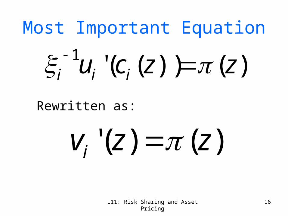
Most Important Equation
)())(('1 zzcu iii
)()(' zzvi Rewritten as:
L11: Risk Sharing and Asset Pricing 17
Limitation• The main weakness of the complete-markets model:
we assume that all individual risks can be traded on financial markets– Labor income risk cannot be traded– Difficult to transfer all of the risk associated with real
estate– Lack of tradability of terrorism risk– If all risks were indeed tradeable, total capitalization of
financial markets must equal the total wealth of the economy.
• Note: Complete market assumption is the cornerstone of modern asset-pricing theory.
L11: Risk Sharing and Asset Pricing 18
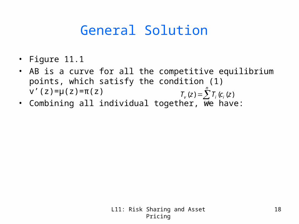
General Solution
• Figure 11.1
• AB is a curve for all the competitive equilibrium points, which satisfy the condition (1) v’(z)=µ(z)=π(z)
• Combining all individual together, we have:
n
iiiv zcTzT
1
))(()(
L11: Risk Sharing and Asset Pricing 19
First Theorem of Welfare Economics
• If there are two states with the same aggregate wealth, the competitive state prices must be the same, and agent I will consume the same amount of consumption good in these two states.
• Individual consumption at equilibrium and competitive state prices depend upon the state only through the aggregate wealth available in the corresponding state. It implies that all the diversifiable risk is eliminated in equilibrium.
• Competitive markets allocate the macroeconomic risk in a Pareto-efficient manner: Decentalized decision making yields efficient sharing.
• The market in aggregation acts like the representative agent in the centralized economy.
L11: Risk Sharing and Asset Pricing 20
Deriving Equity PremiumEquity premium is the difference in the returns of two portfolios: (1) risk-free portfolio and (2) equity portfolio. (1) The risk free portfolio: its price is normalized to 1))(( szE . Note: z(s)=z, referring to units of consumption good delivered by the risk free assets in s. Since
π(.)=v’(.), .1)(' zEv Expressing it differently, .1))(('1
0
szvpS
ss
(2) The equity portfolio: It can be viewed as a portfolio of a constant share α of the aggregate wealth in the economy. The expected return of the portfolio is:
1)('
1)(
zEzv
Ez
zEz
Ez
Agents are risk averse, they require a risk premium. Thus equity premium must be large enough to induce voluntary assumption of the entire aggregate risk.
Using Taylor Expansion, we have ]1[)('')(')(' 200
22000 zzvzzvzzEzv
We thus have 22
0
0 1]1[
z
z
L11: Risk Sharing and Asset Pricing 21
Gauging Equity Premium
• The variance of the yearly growth rate of GDP per capita is around 0.0006 over the last century in the United States. Empirical feasible levels of relative risk aversion is between 1 and 4, then equity premium should be between 0.06% and 0.24% per year.
• However, the observed equity premium has been equal to 6% over that period.
L11: Risk Sharing and Asset Pricing 22
Pricing Individual Assets: Independent Asset Risk
• We now examine the pricing of specific assets within the economy
• The value of risky asset depends on the state of nature that will prevail at the end of the period
• The simplest case: the risk is independent of the market z
• The firm generate a value q with probability p and zero otherwise, i.e., (q,p; 0, 1-p).
• In other words, whatever the GDP z, the firm generates a value q with probability p and zero otherwise.
• When normalizing Eπ(z)=1, we have the expected value of the firm = qp.
L11: Risk Sharing and Asset Pricing 23
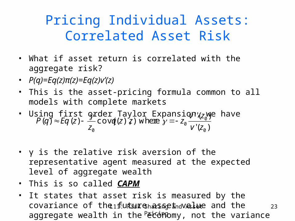
Pricing Individual Assets: Correlated Asset Risk
• What if asset return is correlated with the aggregate risk?
• P(q)=Eq(z)π(z)=Eq(z)v’(z)
• This is the asset-pricing formula common to all models with complete markets
• Using first order Taylor Expansion, we have
• γ is the relative risk aversion of the representative agent measured at the expected level of aggregate wealth
• This is so called CAPM
• It states that asset risk is measured by the covariance of the future asset value and the aggregate wealth in the economy, not the variance of q(z)
)),(cov()()(0
zzqz
zEqqP
where )('
)(''
0
00 zv
zvz
L11: Risk Sharing and Asset Pricing 24
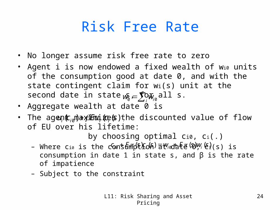
Risk Free Rate
• No longer assume risk free rate to zero
• Agent i is now endowed a fixed wealth of wi0 units of the consumption good at date 0, and with the state contingent claim for wi(s) unit at the second date in state s, for all s.
• Aggregate wealth at date 0 is
• The agent maximizes the discounted value of flow of EU over his lifetime: by choosing optimal ci0, ci(.)– Where ci0 is the consumption at date 0; ci(s) is consumption in date 1 in state
s, and β is the rate of impatience
– Subject to the constraint
i iww 00
))(()( 0 scEucu iiii
)()()()( 00 swsEwscsEc iiii
L11: Risk Sharing and Asset Pricing 25
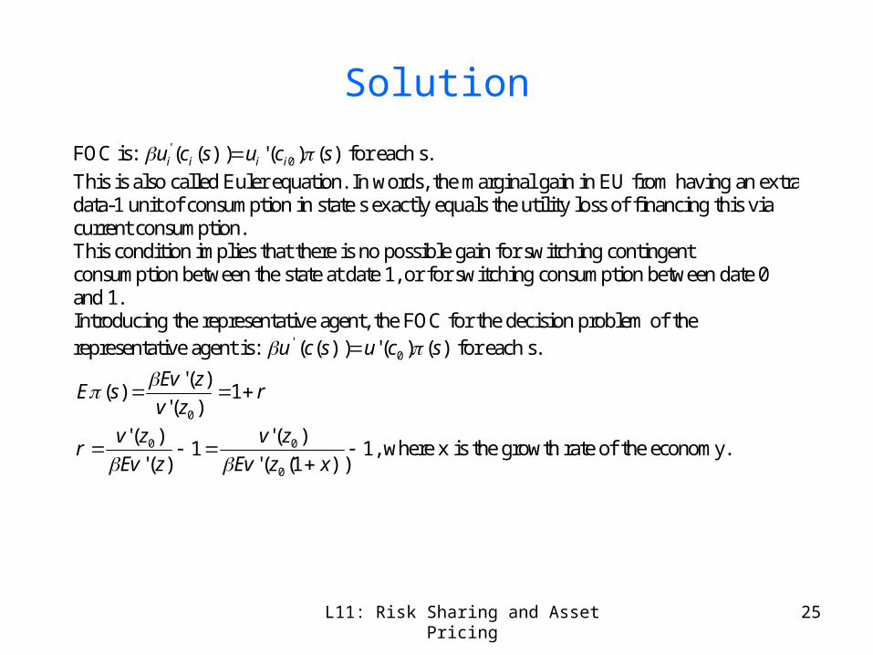
Solution
FOC is: )()('))(( 0' scuscu iiii for each s.
This is also called Euler equation. In words, the marginal gain in EU from having an extra data-1 unit of consumption in state s exactly equals the utility loss of financing this via current consumption. This condition implies that there is no possible gain for switching contingent consumption between the state at date 1, or for switching consumption between date 0 and 1. Introducing the representative agent, the FOC for the decision problem of the representative agent is: )()('))(( 0
' scuscu for each s.
rzv
zEvsE 1
)('
)(')(
0
1))1(('
)('1
)('
)('
0
00
xzEv
zv
zEv
zvr
, where x is the growth rate of the economy.
L11: Risk Sharing and Asset Pricing 26
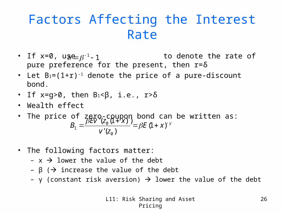
Factors Affecting the Interest Rate
• If x=0, use to denote the rate of pure preference for the present, then r=δ
• Let B1=(1+r)-1 denote the price of a pure-discount bond.
• If x=g>0, then B1<β, i.e., r>δ
• Wealth effect
• The price of zero-coupon bond can be written as:
• The following factors matter:– x lower the value of the debt
– β ( increase the value of the debt
– γ (constant risk aversion) lower the value of the debt
11
)1()('
))1(('
0
01 xE
zv
xzEvB
L11: Risk Sharing and Asset Pricing 27
Exercises
• EGS, 10.1; 10.4; 10.5; 11.1; 11.5