Embed Size (px)
Citation preview

The Annals of Statistics2011, Vol. 39, No. 1, 82–130DOI: 10.1214/10-AOS827© Institute of Mathematical Statistics, 2011
�1-PENALIZED QUANTILE REGRESSION IN HIGH-DIMENSIONALSPARSE MODELS1
BY ALEXANDRE BELLONI AND VICTOR CHERNOZHUKOV
Duke University and Massachusetts Institute of Technology
We consider median regression and, more generally, a possibly infinitecollection of quantile regressions in high-dimensional sparse models. In thesemodels, the number of regressors p is very large, possibly larger than the sam-ple size n, but only at most s regressors have a nonzero impact on each con-ditional quantile of the response variable, where s grows more slowly than n.Since ordinary quantile regression is not consistent in this case, we consider�1-penalized quantile regression (�1-QR), which penalizes the �1-norm ofregression coefficients, as well as the post-penalized QR estimator (post-�1-QR), which applies ordinary QR to the model selected by �1-QR. First, weshow that under general conditions �1-QR is consistent at the near-oracle rate√
s/n√
log(p ∨ n), uniformly in the compact set U ⊂ (0,1) of quantile in-dices. In deriving this result, we propose a partly pivotal, data-driven choiceof the penalty level and show that it satisfies the requirements for achievingthis rate. Second, we show that under similar conditions post-�1-QR is con-sistent at the near-oracle rate
√s/n
√log(p ∨ n), uniformly over U , even if
the �1-QR-selected models miss some components of the true models, and therate could be even closer to the oracle rate otherwise. Third, we characterizeconditions under which �1-QR contains the true model as a submodel, andderive bounds on the dimension of the selected model, uniformly over U ; wealso provide conditions under which hard-thresholding selects the minimaltrue model, uniformly over U .
1. Introduction. Quantile regression is an important statistical method for an-alyzing the impact of regressors on the conditional distribution of a response vari-able (cf. [21, 23]). It captures the heterogeneous impact of regressors on differentparts of the distribution [8], exhibits robustness to outliers [19], has excellent com-putational properties [28], and has wide applicability [19]. The asymptotic theoryfor quantile regression has been developed under both a fixed number of regressorsand an increasing number of regressors. The asymptotic theory under a fixed num-ber of regressors is given in [13, 15, 17, 21, 27] and others. The asymptotic theoryunder an increasing number of regressors is given in [16] and [1, 4], covering thecase where the number of regressors p is negligible relative to the sample size n
[i.e., p = o(n)].
Received December 2009; revised April 2010.1Supported by the NSF Grant SES-0752266.AMS 2000 subject classifications. Primary 62H12, 62J99; secondary 62J07.Key words and phrases. Median regression, quantile regression, sparse models.
82
PENALIZED QUANTILE REGRESSION 83
In this paper, we consider quantile regression in high-dimensional sparse mod-els (HDSMs). In such models, the overall number of regressors p is very large,possibly much larger than the sample size n. However, the number of significant re-gressors for each conditional quantile of interest is at most s, which is smaller thanthe sample size, that is, s = o(n). HDSMs [7, 12, 26] have emerged to deal withmany new applications arising in biometrics, signal processing, machine learning,econometrics, and other areas of data analysis where high-dimensional data setshave become widely available.
A number of papers have begun to investigate estimation of HDSMs, focus-ing primarily on penalized mean regression, with the �1-norm acting as a penaltyfunction [7, 12, 22, 26, 32, 34]. References [7, 12, 22, 26, 34] demonstratedthe fundamental result that �1-penalized least squares estimators achieve the rate√
s/n√
logp, which is very close to the oracle rate√
s/n achievable when the truemodel is known. Reference [32] demonstrated a similar fundamental result on theexcess forecasting error loss under both quadratic and nonquadratic loss functions.Thus, the estimator can be consistent and can have excellent forecasting perfor-mance even under very rapid, nearly exponential, growth of the total number ofregressors p. See [7, 9–11, 14, 25, 29] for many other interesting developmentsand a detailed review of the existing literature.
Our paper’s contribution is to develop a set of results on model selection andrates of convergence for quantile regression within the HDSM framework. Sinceordinary quantile regression is inconsistent in HDSMs, we consider quantile re-gression penalized by the �1-norm of parameter coefficients, denoted �1-QR. First,we show that under general conditions �1-QR estimates of regression coefficientsand regression functions are consistent at the near-oracle rate
√s/n
√log(p ∨ n),
uniformly in a compact interval U ⊂ (0,1) of quantile indices.2 (This result is dif-ferent from, and hence complementary to [32]’s fundamental results on the ratesfor excess forecasting error loss.) Second, in order to make �1-QR practical, wepropose a partly pivotal, data-driven choice of the penalty level, and show that thischoice leads to the same sharp convergence rate. Third, we show that �1-QR cor-rectly selects the true model as a valid submodel when the nonzero coefficients ofthe true model are well separated from zero. Fourth, we also propose and analyzethe post-penalized estimator (post-�1-QR), which applies ordinary, unpenalizedquantile regression to the model selected by the penalized estimator, and thus aimsat reducing the regularization bias of the penalized estimator. We show that un-der similar conditions post-�1-QR can perform as well as �1-QR in terms of therate of convergence, uniformly over U , even if the �1-QR-based model selectionmisses some components of the true models. This occurs because �1-QR-basedmodel selection only misses those components that have relatively small coeffi-cients. Moreover, post-�1-QR can perform better than �1-QR if the �1-QR-based
2Under s → ∞, the oracle rate, uniformly over a proper compact interval U , is√
(s/n) logn,cf. [4]; the oracle rate for a single quantile index is
√s/n; cf. [16].
84 A. BELLONI AND V. CHERNOZHUKOV
model selection correctly includes all components of the true model as a subset.(Obviously, post-�1-QR can perform as well as the oracle if the �1-QR perfectlyselects the true model, which is, however, unrealistic for many designs of interest.)Fifth, we illustrate the use of �1-QR and post-�1-QR with a Monte Carlo experi-ment. To the best of our knowledge, all of the above results are new and contributeto the literature on HDSMs. Our results on post-penalized estimators and someproof techniques could also be of interest in other problems. We provide furthertechnical comparisons to the literature in Section 2.
1.1. Notation. In what follows, we implicitly index all parameter values by thesample size n, but we omit the index whenever this does not cause confusion. Weuse the empirical process notation as defined in [33]. In particular, given a randomsample Z1, . . . ,Zn, let Gn(f ) = Gn(f (Zi)) := n−1/2 ∑n
i=1(f (Zi) − E[f (Zi)])and Enf = Enf (Zi) := ∑n
i=1 f (Zi)/n. We use the notation a � b to denote a =O(b), that is, a ≤ cb for some constant c > 0 that does not depend on n; anda �P b to denote a = OP (b). We also use the notation a ∨ b = max{a, b} anda ∧ b = min{a, b}. We denote the �2-norm by ‖ · ‖, �1-norm by ‖ · ‖1, �∞-norm by‖ · ‖∞ and the �0-“norm” by ‖ · ‖0 (i.e., the number of nonzero components). Wedenote by ‖β‖1,n = ∑p
j=1 σj |βj | the �1-norm weighted by σj ’s. Finally, given avector δ ∈ R
p , and a set of indices T ⊂ {1, . . . , p}, we denote by δT the vector inwhich δTj = δj if j ∈ T , δTj = 0 if j /∈ T .
2. The estimator, the penalty level and overview of rate results. In thissection, we formulate the setting and the estimator, and state primitive regularityconditions. We also provide an overview of the main results.
2.1. Basic setting. The setting of interest corresponds to a parametric quantileregression model, where the dimension p of the underlying model increases withthe sample size n. Namely, we consider a response variable y and p-dimensionalcovariates x such that the uth conditional quantile function of y given x is givenby
F−1yi |xi
(u|xi) = x′β(u), β(u) ∈ Rp for all u ∈ U ,(2.1)
where U ⊂ (0,1) is a compact set of quantile indices. Recall that the uth condi-tional quantile F−1
yi |xi(u|x) is the inverse of the conditional distribution function
Fyi |xi(y|xi) of yi given xi . We consider the case where the dimension p of the
model is large, possibly much larger than the available sample size n, but the truemodel β(u) has a sparse support
Tu = support(β(u)) = {j ∈ {1, . . . , p} : |βj (u)| > 0
}having only su ≤ s ≤ n/ log(n ∨ p) nonzero components for all u ∈ U .
PENALIZED QUANTILE REGRESSION 85
The population coefficient β(u) is known to minimize the criterion function
Qu(β) = E[ρu(y − x′β)],(2.2)
where ρu(t) = (u − 1{t ≤ 0})t is the asymmetric absolute deviation function [21].Given a random sample (y1, x1), . . . , (yn, xn), the quantile regression estimator ofβ(u) is defined as a minimizer of the empirical analog of (2.2):
Qu(β) = En[ρu(yi − x′iβ)].(2.3)
In high-dimensional settings, particularly when p ≥ n, ordinary quantile regres-sion is generally inconsistent, which motivates the use of penalization in order toremove all, or at least nearly all, regressors whose population coefficients are zero,thereby possibly restoring consistency. A penalization that has proven quite usefulin least squares settings is the �1-penalty leading to the Lasso estimator [30].
2.2. Penalized and post-penalized estimators. The �1-penalized quantile re-gression estimator β(u) is a solution to the following optimization problem:
minβ∈Rp
Qu(β) + λ√
u(1 − u)
n
p∑j=1
σj |βj |,(2.4)
where σ 2j = En[x2
ij ]. The criterion function in (2.4) is the sum of the criterion func-tion (2.3) and a penalty function given by a scaled �1-norm of the parameter vector.The overall penalty level λ
√u(1 − u) depends on each quantile index u, while λ
will depend on the set U of quantile indices of interest. The �1-penalized quan-tile regression has been considered in [18] under small (fixed) p asymptotics. It isimportant to note that the penalized quantile regression problem (2.4) is equiva-lent to a linear programming problem (see Appendix C) with a dual version that isuseful for analyzing the sparsity of the solution. When the solution is not unique,we define β(u) as any optimal basic feasible solution (see, e.g., [6]). Therefore,the problem (2.4) can be solved in polynomial time, avoiding the computationalcurse of dimensionality. Our goal is to derive the rate of convergence and modelselection properties of this estimator.
The post-penalized estimator (post-�1-QR) applies ordinary quantile regressionto the model Tu selected by the �1-penalized quantile regression. Specifically, set
Tu = support(β(u)) = {j ∈ {1, . . . , p} : |βj (u)| > 0
},
and define the post-penalized estimator β(u) as
β(u) ∈ arg minβ∈Rp : βT c
u=0
Qu(β),(2.5)
which removes from further estimation the regressors that were not selected. If themodel selection works perfectly—that is, Tu = Tu—then this estimator is simplythe oracle estimator, whose properties are well known. However, perfect model
86 A. BELLONI AND V. CHERNOZHUKOV
selection might be unlikely for many designs of interest. Rather, we are interestedin the more realistic scenario where the first-step estimator β(u) fails to selectsome components of β(u). Our goal is to derive the rate of convergence for thepost-penalized estimator and show it can perform well under this scenario.
2.3. The choice of the penalty level λ. In order to describe our choice of thepenalty level λ, we introduce the random variable
� = n supu∈ U
max1≤j≤p
∣∣∣∣En
[xij (u − 1{ui ≤ u})
σj
√u(1 − u)
]∣∣∣∣,(2.6)
where u1, . . . , un are i.i.d. uniform (0,1) random variables, independently distrib-uted from the regressors, x1, . . . , xn. The random variable � has a known, that is,pivotal, distribution conditional on X = [x1, . . . , xn]′. We then set
λ = c · �(1 − α|X),(2.7)
where �(1 − α|X) := (1 − α)-quantile of � conditional on X, and the constantc > 1 depends on the design.3 Thus, the penalty level depends on the pivotal quan-tity �(1 − α|X) and the design. Under assumptions D.1–D.4, we can set c = 2,similar to [7]’s choice for least squares. Furthermore, we recommend computing�(1 − α|X) using simulation of �.4 Our concrete recommendation for practice isto set 1 − α = 0.9.
The parameter 1 − α is the confidence level in the sense that, as in [7], our(nonasymptotic) bounds on the estimation error will contract at the optimal ratewith this probability. We refer the reader to Koenker [20] for an implementationof our choice of penalty level and practical suggestions concerning the confidencelevel. In particular, both here and in Koenker [20], the confidence level 1 − α =0.9 gave good performance results in terms of balancing regularization bias withestimation variance. Cross-validation may also be used to choose the confidencelevel 1 −α. Finally, we should note that, as in [7], our theoretical bounds allow forany choice of 1 − α and are stated as a function of 1 − α.
The formal rationale behind the choice (2.7) for the penalty level λ is thatthis choice leads precisely to the optimal rates of convergence for �1-QR. (Thesame or slightly higher choice of λ also guarantees good performance of post-�1-QR.) Our general strategy for choosing λ follows [7], who recommend se-lecting λ so that it dominates a relevant measure of noise in the sample crite-rion function, specifically the supremum norm of a suitably rescaled gradient ofthe sample criterion function evaluated at the true parameter value. In our case,
3c depends only on the constant c0 appearing in condition D.4; when c0 ≥ 9, it suffices to setc = 2.
4We also provide analytical bounds on �(1−α|X) of the form C(α, U )√
n logp for some numericconstant C(α, U ). We recommend simulation because it accounts for correlation among the columnsof X in the sample.
PENALIZED QUANTILE REGRESSION 87
this general strategy leads precisely to the choice (2.7). Indeed, a (sub)gradientSu(β(u)) = En[(u − 1{yi ≤ x′
iβ(u)})xi] ∈ ∂Qu(β(u)) of the quantile regressionobjective function evaluated at the truth has a pivotal representation, namelySu(β(u)) = En[(u − 1{ui ≤ u})xi] for u1, . . . , un i.i.d. uniform (0,1) conditionalon X, and so we can represent � as in (2.6), and, thus, choose λ as in (2.7).
2.4. General regularity conditions. We consider the following conditions ona sequence of models indexed by n with parameter dimension p = pn → ∞. Inthese conditions, all constants can depend on n, but we omit the explicit indexingby n to ease exposition.
D.1 (Sampling and smoothness). Data (yi, x′i )
′, i = 1, . . . , n, are an i.i.d. se-quence of real (1 + p)-vectors, with the conditional u-quantile function given by(2.1) for each u ∈ U , with the first component of xi equal to one, and n∧p ≥ 3. Foreach value x in the support of xi , the conditional density fyi |xi
(y|x) is continuouslydifferentiable in y at each y ∈ R, and fyi |xi
(y|x) and ∂∂y
fyi |xi(y|x) are bounded in
absolute value by constants f and f ′, uniformly in y ∈ R and x in the support xi .Moreover, the conditional density of yi evaluated at the conditional quantile x′
iβ(u)
is bounded away from zero uniformly in U , that is, fyi |xi(x′β(u)|x) > f > 0 uni-
formly in u ∈ U and x in the support of xi .
Condition D.1 imposes only mild smoothness assumptions on the conditionaldensity of the response variable given regressors, and does not impose any normal-ity or homoscedasticity assumptions. The assumption that the conditional densityis bounded below at the conditional quantile is standard, but we can replace it bythe slightly more general condition infu∈ U infδ =0(δ
′Juδ)/(δ′E[xix
′i]δ) ≥ f > 0, on
the Jacobian matrices
Ju = E[fyi |xi(x′
iβ(u)|xi)xix′i] for all u ∈ U ,
throughout the paper; see [3] for a further generalization.
D.2 [Sparsity and smoothness of u �→ β(u)]. Let U be a compact subset of(0,1). The coefficients β(u) in (2.1) are sparse and smooth with respect to u ∈ U :
supu∈ U
‖β(u)‖0 ≤ s and ‖β(u) − β(u′)‖ ≤ L|u − u′| for all u,u′ ∈ U ,
where s ≥ 1, and logL ≤ CL log(p ∨ n) for some constant CL.
Condition D.2 imposes sparsity and smoothness on the behavior of the quantileregression coefficients β(u) as we vary the quantile index u.
D.3 (Well-behaved covariates). Covariates are normalized such that σ 2j =
E[x2ij ] = 1 for all j = 1, . . . , p, and σ 2
j = En[x2ij ] obeys P(max1≤j≤p|σj − 1| ≤
1/2) ≥ 1 − γ → 1 as n → ∞.
88 A. BELLONI AND V. CHERNOZHUKOV
Condition D.3 requires that σj does not deviate too much from σj and normal-izes σ 2
j = 1.In order to state the next assumption, for some c0 ≥ 0 and each u ∈ U , define
Au := {δ ∈ Rp :‖δT c
u‖1 ≤ c0‖δTu‖1,‖δT c
u‖0 ≤ n},
which will be referred to as the restricted set. Define T u(δ,m) ⊂ {1, . . . , p} \Tu asthe support of the m largest in absolute value components of the vector δ outsideof Tu = support(β(u)), where T u(δ,m) is the empty set if m = 0.
D.4 (Restricted identifiability and nonlinearity). For some constants m ≥ 0and c0 ≥ 9, the matrix E[xix
′i] satisfies
κ2m := inf
u∈ Uinf
δ∈Au,δ =0
δ′E[xix′i]δ
‖δTu∪T u(δ,m)‖2 > 0(RE(c0,m))
and log(f κ20 ) ≤ Cf log(n ∨ p) for some constant Cf . Moreover,
q := 3
8
f 3/2
f ′ infu∈ U
infδ∈Au,δ =0
E[|x′iδ|2]3/2
E[|x′iδ|3]
> 0.(RNI(c0))
The restricted eigenvalue (RE) condition is analogous to the condition in [7]and [12]; see [7] and [12] for different sufficient primitive conditions that yieldbounds on κm. Also, since κm is nonincreasing in m, (RE(c0,m)) for any m > 0implies (RE(c0,0)). The restricted nonlinear impact (RNI) coefficient q appearingin D.4 is a new concept, which controls the quality of minoration of the quantileregression objective function by a quadratic function over the restricted set.
Finally, we state another condition needed to derive results on the post-modelselected estimator. In order to state the condition, define the sparse set Au(m) ={δ ∈ R
p :‖δT cu‖0 ≤ m} for m ≥ 0 and u ∈ U .
D.5 (Sparse identifiability and nonlinearity). The matrix E[xix′i] satisfies for
some m ≥ 0
κ2m := inf
u∈ Uinf
δ∈Au(m),δ =0
δ′E[xix′i]δ
δ′δ> 0(SE(m))
and
qm := 3
8
f 3/2
f ′ infu∈ U
infδ∈Au(m),δ =0
E[|x′iδ|2]3/2
E[|x′iδ|3]
> 0.(SNI(m))
We invoke the sparse eigenvalue (SE) condition in order to analyze the post-penalized estimator (2.5). This assumption is similar to the conditions used in [26]and [34] to analyze Lasso. Our form of the (SE) condition is neither less nor moregeneral than the (RE) condition. The SNI coefficient qm controls the quality ofminoration of the quantile regression objective function by a quadratic functionover sparse neighborhoods of the true parameter.
PENALIZED QUANTILE REGRESSION 89
2.5. Examples of simple sufficient conditions. In order to highlight the natureand usefulness of conditions D.1–D.5, it is instructive to state some simple suffi-cient conditions (note that D.1–D.5 allow for much more general conditions). Werelegate the proofs of this section to [2] for brevity.
DESIGN 1 (Location model with correlated normal design). Let us considerestimating a standard location model
y = x′βo + ε,
where ε ∼ N(0, σ 2), σ > 0 is fixed, x = (1, z′)′, with z ∼ N(0,�), where � hasones in the diagonal, a minimum eigenvalue bounded away from zero by a constantκ2 > 0, and a maximum eigenvalue bounded from above, uniformly in n.
LEMMA 1. Under Design 1 with U = [ξ,1 − ξ ], ξ > 0, conditions D.1–D.5are satisfied with
f = 1/[√
2πσ], f ′ =
√e/[2π ]/σ 2, f = 1/
√2πξσ,
‖β(u)‖0 ≤ ‖βo‖0 + 1, γ = 2p exp(−n/24), L = σ/ξ,
κm ∧ κm ≥ κ, q ∧ qm ≥ (3/[32ξ3/4])√√
2πσ/e.
Note that the normality of errors can be easily relaxed by allowing for the dis-turbance ε to have a smooth density that obeys the conditions stated in D.1. Theconditions on the population design matrix can also be replaced by more generalprimitive conditions specified in Remark 2.1.
DESIGN 2 (Location-scale model with bounded regressors). Let us considerestimating a standard location-scale model
y = x′βo + x′η · ε,where ε ∼ F independent of x, with a continuously differentiable probability den-sity function f . We assume that the population design matrix E[xx′] has onesin the diagonal and has eigenvalues uniformly bounded away from zero andfrom above, x1 = 1, max1≤j≤p |xj | ≤ KB . Moreover, the vector η is such that0 < υ ≤ x′η ≤ ϒ < ∞ for all values of x.
LEMMA 2. Under Design 2 with U = [ξ,1 − ξ ], ξ > 0, conditions D.1–D.5are satisfied with
f ≤ maxε
f (ε)/υ, f ′ ≤ maxε
f ′(ε)/υ2,
f = minu∈ U
f (F−1(u))/ϒ, ‖β(u)‖0 ≤ ‖βo‖0 + ‖η‖0 + 1,

90 A. BELLONI AND V. CHERNOZHUKOV
γ = 2p exp(−n/[8K4B]), κm ∧ κm ≥ κ, L = ‖η‖f ,
q ≥ 3
8
f 3/2
f ′ κ/[10KB
√s], qm ≥ 3
8
f 3/2
f ′ κ/[KB
√s + m
].
COMMENT 2.1 (Conditions on E[xix′i]). The conditions on the population
design matrix can also be replaced by more general primitive conditions of theform stated in [7] and [12]. For example, conditions on sparse eigenvalues sufficeas shown in [7]. Denote the minimum and maximum eigenvalue of the populationdesign matrix by
ϕmin(m) = min‖δ‖=1,‖δ‖0≤m
δ′E[xix′i]δ
δ′δand
(2.8)
ϕmax(m) = max‖δ‖=1,‖δ‖0≤m
δ′E[xix′i]δ
δ′δ.
Assuming that for some m ≥ s we have mϕmin(m + s) ≥ c20sϕmax(m), then
κm ≥ √ϕmin(s + m)
(1 − c0
√sϕmax(s)/[mϕmin(s + m)])
and
κm ≥ ϕmin(s + m).
2.6. Overview of main results. Here, we discuss our results under the simplesetup of Design 1 and under 1/p ≤ α → 0 and γ → 0. These simple assumptionsallow us to straightforwardly compare our rate results to those obtained in the lit-erature. We state our more general nonasymptotic results under general conditionsin the subsequent sections. Our first main rate result is that �1-QR, with our choice(2.7) of parameter λ, satisfies
supu∈ U
‖β(u) − β(u)‖ �P
1
f κ0κs
√s log(n ∨ p)
n,(2.9)
provided that the upper bound on the number of nonzero components s satisfies√
s log(n ∨ p)√nf 1/2κ0q
→ 0.(2.10)
Note that κ0, κs , f and q are bounded away from zero in this example. Therefore,the rate of convergence is
√s/n · √
log(n ∨ p) uniformly in the set of quantileindices u ∈ U , which is very close to the oracle rate when p grows polynomiallyin n. Further, we note that our resulting restriction (2.10) on the dimension s of thetrue models is very weak; when p is polynomial in n, s can be of almost the sameorder as n, namely s = o(n/ logn).
PENALIZED QUANTILE REGRESSION 91
Our second main result is that the dimension ‖β(u)‖0 of the model selected bythe �1-penalized estimator is of the same stochastic order as the dimension s of thetrue models, namely
supu∈ U
‖β(u)‖0 �P s.(2.11)
Further, if the parameter values of the minimal true model are well separated fromzero, then with a high probability the model selected by the �1-penalized estimatorcorrectly nests the true minimal model:
Tu = support(β(u)) ⊆ Tu = support(β(u)) for all u ∈ U .(2.12)
Moreover, we provide conditions under which a hard-thresholded version of theestimator selects the correct support.
Our third main result is that the post-penalized estimator, which applies ordinaryquantile regression to the selected model, obeys
supu∈ U
‖β(u) − β(u)‖ �P
1
f κ2m
√m log(n ∨ p) + s logn
n(2.13)
+ supu∈ U 1{Tu ⊆ Tu}f κ0κm
√s log(n ∨ p)
n,
where m = supu∈ U ‖βT cu(u)‖0 is the maximum number of wrong components se-
lected for any quantile index u ∈ U , provided that the bound on the number ofnonzero components s obeys the growth condition (2.10) and
√m log(n ∨ p) + s logn√
nf 1/2κmqm
→P 0.(2.14)
[Note that when U is a singleton, the s logn factor in (2.13) becomes s.]We see from (2.13) that post-�1-QR can perform well in terms of the rate of
convergence even if the selected model Tu fails to contain the true model Tu.Indeed, since in this design m �P s, post-�1-QR has the rate of convergence√
s/n · √log(n ∨ p), which is the same as the rate of convergence of �1-QR. Theintuition for this result is that the �1-QR based model selection can only miss co-variates with relatively small coefficients, which then permits post-�1-QR to per-form as well or even better due to reductions in bias, as confirmed by our compu-tational experiments.
We also see from (2.13) that post-�1-QR can perform better than �1-QR in termsof the rate of convergence if the number of wrong components selected obeysm = oP (s) and the selected model contains the true model, {Tu ⊆ Tu} with prob-ability converging to one. In this case, post-�1-QR has the rate of convergence√
(oP (s)/n) log(n ∨ p) + (s/n) logn, which is faster than the rate of convergenceof �1-QR. In the extreme case of perfect model selection, that is, when m = 0, the
92 A. BELLONI AND V. CHERNOZHUKOV
rate of post-�1-QR becomes√
(s/n) logn uniformly in U . (When U is a single-ton, the logn factor drops out.) Note that inclusion {Tu ⊆ Tu} necessarily happenswhen the coefficients of the true models are well separated from zero, as we statedabove. Note also that the condition m = o(s) or even m = 0 could occur underadditional conditions on the regressors (such as the mutual coherence conditionsthat restrict the maximal pairwise correlation of regressors). Finally, we note thatour second restriction (2.14) on the dimension s of the true models is very weakin this design; when p is polynomial in n, s can be of almost the same order as n,namely s = o(n/ logn).
To the best of our knowledge, all of the results presented above are new, bothfor the single �1-penalized quantile regression problem as well as for the infinitecollection of �1-penalized quantile regression problems. These results thereforecontribute to the rate results obtained for �1-penalized mean regression and re-lated estimators in the fundamental papers of [7, 12, 22, 26, 32, 34]. The resultson post-�1 penalized quantile regression had no analogs in the literature on meanregression, apart from the rather exceptional case of perfect model selection, inwhich case the post-penalized estimator is simply the oracle. Building on the cur-rent work these results have been extended to mean regression in [5]. Our resultson the sparsity of �1-QR and model selection also contribute to the analogous re-sults for mean regression [26]. Also, our rate results for �1-QR are different from,and hence complementary to, the fundamental results in [32] on the excess fore-casting loss under possibly nonquadratic loss functions, which also specializes theresults to density estimation, mean regression, and logistic regression. In princi-ple, we could apply theorems in [32] to the single quantile regression problem toderive the bounds on the excess loss E[ρu(yi − x′
i β(u))] − E[ρu(yi − x′iβ(u))].5
However, these bounds would not imply our results (2.7), (2.9), (2.11), (2.12) and(2.13), which characterize the rates of estimating coefficients β(u) by �1-QR andpost-�1-QR, sparsity and model selection properties, and the data-driven choice ofthe penalty level.
3. Main results and main proofs. In this section, we derive rates of conver-gence for �1-QR and post-�1-QR, sparsity bounds, and model selection results.
3.1. Bounds on �(1 − α|X). We start with a characterization of � and its(1 − α)-quantile, �(1 − α|X), which determines the magnitude of our suggestedpenalty level λ via equation (2.7).
5Of course, such a derivation would entail some difficult work, since we must verify some high-level assumptions made directly on the performance of the oracle and penalized estimators in popu-lation and others (cf. [32], conditions I.1 and I.2, where I.2 assumes uniform in xi consistency of thepenalized estimator in the population, and does not hold in our main examples, e.g., in Design 1 withnormal regressors).
PENALIZED QUANTILE REGRESSION 93
THEOREM 1 [Bounds on �(1 − α|X)]. Let WU = maxu∈ U 1/√
u(1 − u).There is a universal constant C� such that:
(i) P(� ≥ k · C�WU√
n logp|X) ≤ p−k2+1,(ii) �(1 − α|X) ≤ √
1 + log(1/α)/ logp · C�WU√
n logp with probability 1.
3.2. Rates of convergence. In this section, we establish the rate of convergenceof �1-QR. We start with the following preliminary result which shows that if thepenalty level exceeds the specified threshold, for each u ∈ U , the estimator β(u)−β(u) will belong to the restricted set Au := {δ ∈ R
p :‖δT cu‖1 ≤ c0‖δTu‖1,‖δT c
u‖0 ≤
n}.
LEMMA 3 (Restricted set). 1. Under D.3, with probability at least 1 − γ wehave for every δ ∈ R
p that
23‖δ‖1,n ≤ ‖δ‖1 ≤ 2‖δ‖1,n.(3.1)
2. Moreover, if for some α ∈ (0,1)
λ ≥ λ0 := c0 + 3
c0 − 3�(1 − α|X),(3.2)
then with probability at least 1 − α − γ , uniformly in u ∈ U , we have (3.1) and
β(u) − β(u) ∈ Au = {δ ∈ Rp :‖δT c
u‖1 ≤ c0‖δTu‖1,‖δT c
u‖0 ≤ n}.
This result is inspired by the analogous result for least squares in [7].
LEMMA 4 (Identifiability relations over restricted set). Condition D.4, namely(RE(c0,m)) and (RNI(c0)), implies that for any δ ∈ Au and u ∈ U ,
‖(E[xix′i])1/2δ‖ ≤ ‖J 1/2
u δ‖/f 1/2,(3.3)
‖δTu‖1 ≤ √s‖J 1/2
u δ‖/[f 1/2κ0],(3.4)
‖δ‖1 ≤ √s(1 + c0)‖J 1/2
u δ‖/[f 1/2κ0],(3.5)
‖δ‖ ≤ (1 + c0
√s/m
)‖J 1/2u δ‖/[f 1/2κm],(3.6)
Qu
(β(u) + δ
)− Qu(β(u)) ≥ (‖J 1/2u δ‖2/4) ∧ (q‖J 1/2
u δ‖).(3.7)
This second preliminary result derives identifiability relations over Au. It showsthat the coefficients f , κ0 and κm control moduli of continuity between variousnorms over the restricted set Au, and the RNI coefficient q controls the quality ofminoration of the objective function by a quadratic function over Au.
Finally, the third preliminary result derives bounds on the empirical errorover Au.
94 A. BELLONI AND V. CHERNOZHUKOV
LEMMA 5 (Control of empirical error). Under D.1–D.4, for any t > 0 let
ε(t) := supu∈ U ,δ∈Au,‖J 1/2
u δ‖≤t
∣∣Qu
(β(u) + δ
)− Qu
(β(u) + δ
)− (
Qu(β(u)) − Qu(β(u)))∣∣.
Then, there is a universal constant CE such that for any A > 1, with probability atleast 1 − 3γ − 3p−A2
ε(t) ≤ t · CE · (1 + c0)A
f 1/2κ0
√s log(p ∨ [Lf 1/2κ0/t])
n.
In order to prove the lemma, we use a combination of chaining arguments andexponential inequalities for contractions [24]. Our use of the contraction principleis inspired by its fundamentally innovative use in [32]; however, the use of thecontraction principle alone is not sufficient in our case. Indeed, first we need tomake some adjustments to obtain error bounds over the neighborhoods defined bythe intrinsic norm ‖J 1/2
u · ‖ instead of the ‖ · ‖1 norm; and second, we need to usechaining over u ∈ U to get uniformity over U .
Armed with Lemmas 3–5, we establish the first main result. The result dependson the constants C�, CE , CL and Cf defined in Theorem 1, Lemma 5, condi-tions D.2 and D.4.
THEOREM 2 (Uniform bounds on estimation error of �1-QR). Assume condi-tions D.1–D.4 hold, and let
C > 2C�
√1 + log(1/α)/ logp ∨ [
CE
√1 ∨ [CL + Cf + 1/2]].
Let λ0 be defined as in (3.2). Then uniformly in the penalty level λ such that
λ0 ≤ λ ≤ C · WU√
n logp,(3.8)
we have that, for any A > 1 with probability at least 1 − α − 4γ − 3p−A2,
supu∈ U
∥∥J 1/2u
(β(u) − β(u)
)∥∥ ≤ 8C · (1 + c0)WU A
f 1/2κ0·√
s log(p ∨ n)
n,
supu∈ U
√Ex
[x′(β(u) − β(u)
)]2 ≤ 8C · (1 + c0)WU A
f κ0·√
s log(p ∨ n)
n
and
supu∈ U
‖β(u) − β(u)‖ ≤ 1 + c0√
s/m
κm
· 8C · (1 + c0)WU A
f κ0·√
s log(p ∨ n)
n,
PENALIZED QUANTILE REGRESSION 95
provided s obeys the growth condition
2C · (1 + c0)WU A ·√
s log(p ∨ n) < qf 1/2κ0√
n.(3.9)
This result derives the rate of convergence of the �1-penalized quantile regres-sion estimator in the intrinsic norm and other norms of interest uniformly in u ∈ Uas well as uniformly in the penalty level λ in the range specified by (3.8), whichincludes our recommended choice of λ0. We see that the rates of convergence for�1-QR generally depend on the number of significant regressors s, the logarithmof the number of regressors p, the strength of identification summarized by κ0, κm,f and q , and the quantile indices of interest U (as expected, extreme quantiles canslow down the rates of convergence). These rate results parallel the results of [7]obtained for �1-penalized mean regression. Indeed, the role of the parameter f issimilar to the role of the standard deviation of the disturbance in mean regression. Itis worth noting, however, that our results do not rely on normality and homoscedas-ticity assumptions, and our proofs have to address the nonquadratic nature of theobjective function, with parameter q controlling the quality of quadratization. Thisparameter q enters the results only through the growth restriction (3.9) on s. At thispoint, we refer the reader to Section 2.4 for a further discussion of this result inthe context of the correlated normal design. Finally, we note that our proof com-bines the star-shaped geometry of the restricted set Au with classical convexityarguments; this insight may be of interest in other problems.
PROOF OF THEOREM 2. We let
t := 8C · (1 + c0)WU A
f 1/2κ0·√
s log(p ∨ n)
n
and consider the following events:
(i) �1 := the event that (3.1) and β(u)−β(u) ∈ Au, uniformly in u ∈ U , hold;(ii) �2 := the event that the bound on empirical error ε(t) in Lemma 5 holds;
(iii) �3 := the event in which �(1 − α|X) ≤ √1 + log(1/α)/ logp · C�WU ×√
n logp.
By the choice of λ and Lemma 3, P(�1) ≥ 1 − α − γ ; by Lemma 5 P(�2) ≥1 − 3γ − 3p−A2
; and by Theorem 1 P(�3) = 1, hence P(⋂3
k=1 �k) ≥ 1 − α −4γ − 3p−A2
.Given the event
⋂3k=1 �k , we want to show the event that
∃u ∈ U∥∥J 1/2
u
(β(u) − β(u)
)∥∥ > t(3.10)
is impossible, which will prove the first bound. The other two bounds then followfrom Lemma 4 and the first bound. First, note that the event in (3.10) implies that
96 A. BELLONI AND V. CHERNOZHUKOV
for some u ∈ U0 > min
δ∈Au,‖J 1/2u δ‖≥t
Qu
(β(u) + δ
)− Qu(β(u))
+ λ√
u(1 − u)
n
(‖β(u) + δ‖1,n − ‖β(u)‖1,n
).
The key observation is that by convexity of Qu(·) + ‖ · ‖1,nλ√
u(1 − u)/n and bythe fact that Au is a cone, we can replace ‖J 1/2
u δ‖ ≥ t by ‖J 1/2u δ‖ = t in the above
inequality and still preserve it:
0 > minδ∈Au,‖J 1/2
u δ‖=t
Qu
(β(u) + δ
)− Qu(β(u))
+ λ√
u(1 − u)
n
(‖β(u) + δ‖1,n − ‖β(u)‖1,n
).
Also, by inequality (3.4) in Lemma 4, for each δ ∈ Au
‖β(u)‖1,n − ‖β(u) + δ‖1,n ≤ ‖δTu‖1,n ≤ 2‖δTu‖1 ≤ 2√
s‖J 1/2u δ‖/f 1/2κ0,
which then further implies
0 > minδ∈Au,‖J 1/2
u δ‖=t
Qu
(β(u) + δ
)− Qu(β(u))
(3.11)
− λ√
u(1 − u)
n
2√
s
f 1/2κ0‖J 1/2
u δ‖.
Also by Lemma 5, under our choice of t ≥ 1/[f 1/2κ0√
n], log(Lf κ20 ) ≤ (CL +
Cf ) log(n ∨ p), and under event �2
ε(t) ≤ tCE
√1 ∨ [CL + Cf + 1/2](1 + c0)A
f 1/2κ0
√s log(p ∨ n)
n.(3.12)
Therefore, we obtain from (3.11) and (3.12)
0 ≥ minδ∈Au,‖J 1/2
u δ‖=t
Qu
(β(u) + δ
)− Qu(β(u)) − λ√
u(1 − u)
n
2√
s
f 1/2κ0‖J 1/2
u δ‖
− tCE
√1 ∨ [CL + Cf + 1/2](1 + c0)A
f 1/2κ0
√s log(p ∨ n)
n.
Using the identifiability relation (3.7) stated in Lemma 4, we further get
0 >t2
4∧ (qt) − t
λ√
u(1 − u)
n
2√
s
f 1/2κ0
− tCE
√1 ∨ [CL + Cf + 1/2](1 + c0)A
f 1/2κ0
√s log(p ∨ n)
n.
PENALIZED QUANTILE REGRESSION 97
Using the upper bound on λ under event �3, we obtain
0 >t2
4∧ (qt) − tC
2√
s logp√n
WU
f 1/2κ0
− tCE
√1 ∨ [CL + Cf + 1/2](1 + c0)A
f 1/2κ0
√s log(p ∨ n)
n.
Note that qt cannot be smaller than t2/4 under the growth condition (3.9) in thetheorem. Thus, using also the lower bound on C given in the theorem, WU ≥ 1,and c0 ≥ 1, we obtain the relation
0 >t2
4− t · 2C
(1 + c0)WU A
f 1/2κ0·√
s log(p ∨ n)
n= 0,
which is impossible. �
3.3. Sparsity properties. Next, we derive sparsity properties of the solution to�1-penalized quantile regression. Fundamentally, sparsity is linked to the first or-der optimality conditions of (2.4) and therefore to the (sub)gradient of the criterionfunction. In the case of least squares, the gradient is a smooth (linear) function ofthe parameters. In the case of quantile regression, the gradient is a highly non-smooth (piece-wise constant) function. To control the sparsity of β(u), we relyon empirical process arguments to approximate gradients by smooth functions. Inparticular, we crucially exploit the fact that the entropy of all m-dimensional sub-models of the p-dimensional model is of order m logp, which depends on p onlylogarithmically.
The statement of the results will depend on the maximal k-sparse eigenvalue ofE[xix
′i] and En[xix
′i]:
ϕmax(k) = maxδ =0,‖δ‖0≤k
E[(x′iδ)
2]δ′δ
and
(3.13)
φ(k) = supδ =0,‖δ‖0≤k
En[(x′iδ)
2]δ′δ
∨ E[(x′iδ)
2]δ′δ
.
In order to establish our main sparsity result, we need two preliminary lemmas.
LEMMA 6 (Empirical pre-sparsity). Let s = supu∈ U ‖β(u)‖0. Under D.1–D.4,for any λ > 0, with probability at least 1 − γ we have
s ≤ n ∧ p ∧ [4n2φ(s)W 2U /λ2].
In particular, if λ ≥ 2√
2WU√
n log(n ∨ p)φ(n/ log(n ∨ p)) then s ≤ n/ log(n ∨p).
98 A. BELLONI AND V. CHERNOZHUKOV
This lemma establishes an initial bound on the number of nonzero componentss as a function of λ and φ(s). Restricting
λ ≥ 2√
2WU√
n log(n ∨ p)φ(n/ log(n ∨ p)
)makes the term φ(n/ log(n ∨ p)) appear in subsequent bounds instead of the termφ(n), which in turn weakens some assumptions. Indeed, not only is the first termsmaller than the second, but also there are designs of interest where the secondterm diverges while the first does not; for instance, in Design 1, if p ≥ 2n, we haveφ(n/ log(n ∨ p)) �P 1 while φ(n) �P
√logp by [2].
The following lemma establishes a bound on the sparsity as a function of therate of convergence.
LEMMA 7 (Empirical sparsity). Assume D.1–D.4 and let
r = supu∈ U
∥∥J 1/2u
(β(u) − β(u)
)∥∥.Then, for any ε > 0, there is a constant Kε ≥ √
2 such that with probability at least1 − ε − γ ,
√s
WU≤ μ(s)
n
λ(r ∧ 1) + √
sKε
√n log(n ∨ p)φ(s)
λ,
μ(k) := 2√
ϕmax(k)(1 ∨ 2f /f 1/2).
Finally, we combine these results to establish the main sparsity result. In whatfollows, we define φε as a constant such that φ(n/ log(n∨p)) ≤ φε with probabil-ity 1 − ε.
THEOREM 3 (Uniform sparsity bounds). Let ε > 0 be any constant, assumeD.1–D.4 hold, and let λ satisfy λ ≥ λ0 and
KWU√
n log(n ∨ p) ≤ λ ≤ K ′WU√
n log(n ∨ p)
for some constant K ′ ≥ K ≥ 2Kεφ1/2ε , for Kε defined in Lemma 7. Then, for any
A > 1 with probability at least 1 − α − 2ε − 4γ − p−A2,
s := supu∈ U
‖β(u)‖0 ≤ s · [16μWU /f 1/2κ0]2[(1 + c0)AK ′/K]2,
where μ := μ(n/ log(n ∨ p)), provided that s obeys the growth condition
2K ′(1 + c0)AWU√
s log(n ∨ p) < qf 1/2κ0√
n.(3.14)
PENALIZED QUANTILE REGRESSION 99
The theorem states that by setting the penalty level λ to be possibly higher thanour initial recommended choice λ0, we can control s, which will be crucial forgood performance of the post-penalized estimator. As a corollary, we note that if(a) μ � 1, (b) 1/(f 1/2κ0) � 1 and (c) φε � 1 for each ε > 0, then s � s with ahigh probability, so the dimension of the selected model is about the same as thedimension of the true model. Conditions (a), (b) and (c) easily hold for the corre-lated normal design in Design 1. In particular, (c) follows from the concentrationinequalities and from results in classical random matrix theory; see [2] for proofs.Therefore the possibly higher λ needed to achieve the stated sparsity bound doesnot slow down the rate of �1-QR in this case. The growth condition (3.14) on s isalso weak in this case.
PROOF OF THEOREM 3. By the choice of K and Lemma 6, s ≤ n/ log(n∨p)
with probability 1 − ε. With at least the same probability, the choice of λ yields
Kε
√n log(n ∨ p)φ(s)
λ≤ Kεφ
1/2ε
KWU≤ 1
2WU,
so that by virtue of Lemma 7 and by μ(s) ≤ μ := μ(n/ log(n ∨ p)),√
s
WU≤ μ
(r ∧ 1)n
λ+
√s
2WUor √
s
WU≤ 2μ
(r ∧ 1)n
λ,
with probability 1 − 2ε. Since all conditions of Theorem 2 hold, we obtain theresult by plugging in the upper bound on r = supu∈ U ‖J 1/2
u (β(u) − β(u))‖ fromTheorem 2. �
3.4. Model selection properties. Next, we turn to the model selection proper-ties of �1-QR.
THEOREM 4 (Model selection properties of �1-QR). Let ro = supu∈ U ‖β(u)−β(u)‖. If infu∈ U minj∈Tu |βj (u)| > ro, then
Tu := support(β(u)) ⊆ Tu := support(β(u)) for all u ∈ U .(3.15)
Moreover, the hard-thresholded estimator β(u), defined for any γ ≥ 0 by
βj (u) = βj (u)1{|βj (u)| > γ }, u ∈ U , j = 1, . . . , p,(3.16)
provided that γ is chosen such that ro < γ < infu∈ U minj∈Tu |βj (u)|− ro, satisfies
support(β(u)) = Tu for all u ∈ U .
100 A. BELLONI AND V. CHERNOZHUKOV
These results parallel analogous results in [26] for mean regression. The firstresult says that if nonzero coefficients are well separated from zero, then the sup-port of �1-QR includes the support of the true model. The inclusion of the truesupport in (3.15) is in general one-sided; the support of the estimator can includesome unnecessary components having true coefficients equal to zero. The secondresult states that if the further conditions are satisfied, additional hard thresholdingcan eliminate inclusions of such unnecessary components. The value of the hardthreshold must explicitly depend on the unknown value minj∈Tu |βj (u)|, character-izing the separation of nonzero coefficients from zero. The additional conditionsstated in this theorem are strong and perfect model selection appears quite un-likely in practice. Certainly it does not work in all real empirical examples wehave explored. This motivates our analysis of the post-model-selected estimatorunder conditions that allow for imperfect model selection, including cases wherewe miss some nonzero components or have additional unnecessary components.
3.5. The post-penalized estimator. In this section, we establish a bound on therate of convergence of the post-penalized estimator. The proof relies crucially onthe identifiability and control of the empirical error over the sparse sets Au(m) :={δ ∈ R
p :‖δT cu‖0 ≤ m}.
LEMMA 8 (Sparse identifiability and control of empirical error). 1. Sup-pose D.1 and D.5 hold. Then for all δ ∈ Au(m), u ∈ U , and m ≤ n, we have that
Qu
(β(u) + δ
)− Qu(β(u)) ≥ ‖J 1/2u δ‖2
4∧ (qm‖J 1/2
u δ‖).(3.17)
2. Suppose D.1, D.2 and D.5 hold and that |⋃u∈ U Tu| ≤ n. Then for any ε > 0,there is a constant Cε such that with probability at least 1 − ε the empirical error
εu(δ) := ∣∣Qu
(β(u) + δ
)− Qu
(β(u) + δ
)− (Qu(β(u)) − Qu(β(u))
)∣∣obeys
supu∈ U ,δ∈Au(m),δ =0
εu(δ)
‖δ‖ ≤ Cε
√(m log(n ∨ p) + s logn)φ(m + s)
n
for all m ≤ n.
In order to prove this lemma, we exploit the crucial fact that the entropy of allm-dimensional submodels of the p-dimensional model is of order m logp, whichdepends on p only logarithmically. The following theorem establishes the proper-ties of post-model-selection estimators.
THEOREM 5 (Uniform bounds on estimation error of post-�1-QR). Assumethe conditions of Theorem 2 hold, assume that |⋃u∈ U Tu| ≤ n, and assume D.5
PENALIZED QUANTILE REGRESSION 101
holds with m := supu∈ U ‖βT cu(u)‖0 with probability 1 − ε. Then for any ε > 0
there is a constant Cε such that the bounds
supu∈ U
∥∥J 1/2u
(β(u) − β(u)
)∥∥≤ 4Cε
√φ(m + s)
f 1/2κm
·√
m log(n ∨ p) + s logn
n
+ supu∈ U
1{Tu ⊆ Tu} · 4√
2(1 + c0)A
f 1/2κ0· C · WU
√s log(n ∨ p)
n,(3.18)
supu∈ U
√Ex
[x′(β(u) − β(u)
)]2 ≤ supu∈ U
∥∥J 1/2u
(β(u) − β(u)
)∥∥/f 1/2,
supu∈ U
‖β(u) − β(u)‖ ≤ supu∈ U
∥∥J 1/2u
(β(u) − β(u)
)∥∥/f 1/2κm,
hold with probability at least 1 − α − 3γ − 3p−A2 − 2ε, provided that s obeys thegrowth condition
qm
Cε
√(m log(n ∨ p) + s logn)φ(m + s)√
nf 1/2κm
+ supu∈ U
1{Tu ⊆ Tu}2A(1 + c0) · C2W 2U · s log(p ∨ n)
nf κ20
≤ q2m.
This theorem describes the performance of post-�1-QR. However, an inspectionof the proof reveals that it can be applied to any post-model selection estima-tor. From Theorem 5, we can conclude that in many interesting cases the ratesof post-�1-QR could be the same or faster than the rate of �1-QR. Indeed, firstconsider the case where the model selection fails to contain the true model, thatis, supu∈ U 1{Tu ⊆ Tu} = 1 with a nonnegligible probability. If (a) m ≤ s �P s,(b) φ(m + s) �P 1 and (c) the constants f and κ2
m are of the same order as f andκ0κm, respectively, then the rate of convergence of post-�1-QR is the same as therate of convergence of �1-QR. Recall that Theorem 3 provides sufficient condi-tions needed to achieve (a), which hold in Design 1. Recall also that in Design 1,(b) holds by concentration of measure and classical results in random matrix the-ory, as shown in [2], and (c) holds by the calculations presented in Section 2. Thisverifies our claim regarding the performance of post-�1-QR in the overview, Sec-tion 2.4. The intuition for this result is that even though �1-QR misses true compo-nents, it does not miss very important ones, allowing post-�1-QR still to performwell. Second, consider the case where the model selection succeeds in containingthe true model, that is, supu∈ U 1{Tu ⊆ Tu} = 0 with probability approaching one,and that the number of unnecessary components obeys m = oP (s). In this case,
102 A. BELLONI AND V. CHERNOZHUKOV
the rate of convergence of post-�1-QR can be faster than the rate of convergenceof �1-QR. In the extreme case of perfect model selection, when m = 0 with a highprobability, post-�1-QR becomes the oracle estimator with a high probability. Werefer the reader to Section 2 for further discussion, and note that this result couldbe of interest in other problems.
PROOF OF THEOREM 5. Let
δ(u) = β(u) − β(u), δ(u) := β(u) − β(u), tu := ‖J 1/2u δ(u)‖,
and Bn be a random variable such that Bn = supu∈ U Qu(β(u))−Qu(β(u)). By theoptimality of β(u) in (3.16), with probability 1 − γ we have uniformly in u ∈ U
Qu(β(u)) − Qu(β(u)) ≤ λ√
u(1 − u)
n
(‖β(u)‖1,n − ‖β(u)‖1,n
)≤ λ
√u(1 − u)
n‖δTu(u)‖1,n(3.19)
≤ λ√
u(1 − u)
n2‖δTu(u)‖1,
where the last term in (3.19) is bounded by
λ√
u(1 − u)
n
2√
s‖J 1/2u δ(u)‖
f 1/2κ0(3.20)
≤ λ√
u(1 − u)
n
2√
s
f 1/2κ0supu∈ U
∥∥J 1/2u
(β(u) − β(u)
)∥∥,using that ‖J 1/2
u δ(u)‖ ≥ f 1/2κ0‖δTu(u)‖ from (RE(c0,0)) implied by D.4. There-fore, by Theorem 2 we have
Bn ≤ λ√
u(1 − u)
n
2√
s
f 1/2κ08C · (1 + c0)WU A
f 1/2κ0·√
s log(p ∨ n)
n
with probability 1 − α − 3γ − 3p−A2.
For every u ∈ U , by optimality of β(u) in (2.5),
Qu(β(u)) − Qu(β(u)) ≤ 1{Tu ⊆ Tu}(Qu(β(u)) − Qu(β(u)))
(3.21)≤ 1{Tu ⊆ Tu}Bn.
Also, by Lemma 8, with probability at least 1 − ε, we have
supu∈ U
εu(δ(u))
‖δ(u)‖ ≤ Cε
√(m log(n ∨ p) + s logn)φ(m + s)
n=: Aε,n.(3.22)
PENALIZED QUANTILE REGRESSION 103
Recall that supu∈ U ‖δT cu(u)‖ ≤ m ≤ n so that by D.5 tu ≥ f 1/2κm‖δ(u)‖ for all
u ∈ U with probability 1 − ε. Thus, combining relations (3.21) and (3.22), forevery u ∈ U
Qu(β(u)) − Qu(β(u)) ≤ tuAε,n/[f 1/2κm] + 1{Tu ⊆ Tu}Bn
with probability at least 1 − 2ε. Invoking the sparse identifiability relation (3.17)of Lemma 8, with the same probability, for all u ∈ U ,
(t2u/4) ∧ (qmtu) ≤ tuAε,n/[f 1/2κm] + 1{Tu ⊆ Tu}Bn.
We then conclude that under the assumed growth condition on s, this inequalityimplies
tu ≤ 4Aε,n/[f 1/2κm] + 1{Tu ⊆ Tu}√
4Bn ∨ 0
for every u ∈ U , and the bounds stated in the theorem now follow from the defini-tion of f and κm. �
4. Empirical performance. In order to assess the finite sample practical per-formance of the proposed estimators, we conducted a Monte Carlo study. We willcompare the performance of the �1-penalized, post-�1-penalized and the ideal ora-cle quantile regression estimators. Recall that the post-penalized estimator appliescanonical quantile regression to the model selected by the penalized estimator.The oracle estimator applies canonical quantile regression to the true model. (Ofcourse, such an estimator is not available outside Monte Carlo experiments.) Wefocus our attention on the model selection properties of the penalized estimatorand biases and empirical risks of these estimators.
We begin by considering the following regression model:
y = x′β(0.5) + ε, β(0.5) = (1,1,1/2,1/3,1/4,1/5,0, . . . ,0)′,
where as in Design 1, x = (1, z′)′ consists of an intercept and covariates z ∼N(0,�), and the errors ε are independently and identically distributed ε ∼N(0, σ 2). The dimension p of covariates x is 500, and the dimension s of thetrue model is 6, and the sample size n is 100. We set the regularization parameterλ equal to the 0.9-quantile of the pivotal random variable �, following our pro-posal in Section 2. The regressors are correlated with �ij = ρ|i−j | and ρ = 0.5.We consider two levels of noise, namely σ = 1 and σ = 0.1.
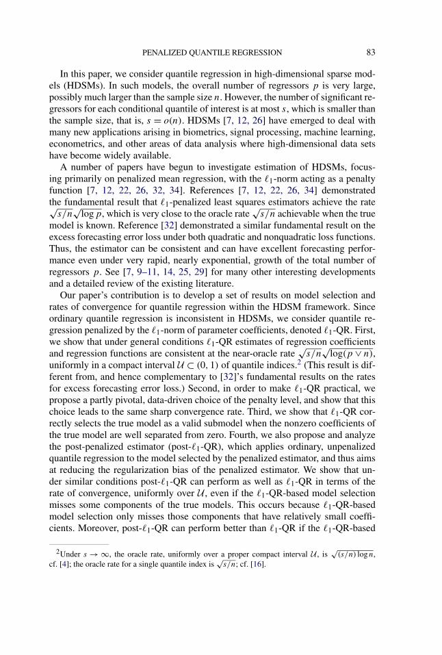
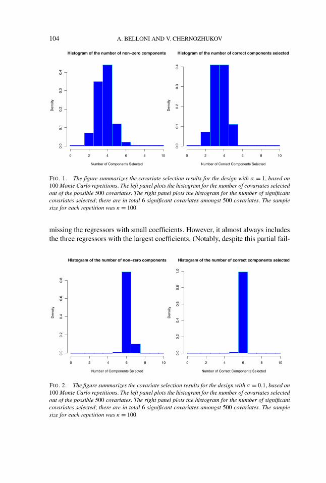
We summarize the model selection performance of the penalized estimator inFigures 1 and 2. In the left panels of the figures, we plot the frequencies of thedimensions of the selected model; in the right panels, we plot the frequencies ofselecting the correct regressors. From the left panels, we see that the frequencyof selecting a much larger model than the true model is very small in both de-signs. In the design with a larger noise, as the right panel of Figure 1 shows, thepenalized quantile regression never selects the entire true model correctly, always
104 A. BELLONI AND V. CHERNOZHUKOV
FIG. 1. The figure summarizes the covariate selection results for the design with σ = 1, based on100 Monte Carlo repetitions. The left panel plots the histogram for the number of covariates selectedout of the possible 500 covariates. The right panel plots the histogram for the number of significantcovariates selected; there are in total 6 significant covariates amongst 500 covariates. The samplesize for each repetition was n = 100.
missing the regressors with small coefficients. However, it almost always includesthe three regressors with the largest coefficients. (Notably, despite this partial fail-
FIG. 2. The figure summarizes the covariate selection results for the design with σ = 0.1, based on100 Monte Carlo repetitions. The left panel plots the histogram for the number of covariates selectedout of the possible 500 covariates. The right panel plots the histogram for the number of significantcovariates selected; there are in total 6 significant covariates amongst 500 covariates. The samplesize for each repetition was n = 100.
PENALIZED QUANTILE REGRESSION 105
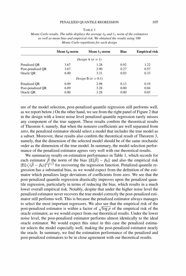
TABLE 1Monte Carlo results. The table displays the average �0 and �1 norm of the estimators
as well as mean bias and empirical risk. We obtained the results using 100Monte Carlo repetitions for each design
Mean �0-norm Mean �1-norm Bias Empirical risk
Design A (σ = 1)
Penalized QR 3.67 1.28 0.92 1.22Post-penalized QR 3.67 2.90 0.27 0.57Oracle QR 6.00 3.31 0.03 0.33
Design B (σ = 0.1)
Penalized QR 6.09 2.98 0.13 0.19Post-penalized QR 6.09 3.28 0.00 0.04Oracle QR 6.00 3.28 0.00 0.03
ure of the model selection, post-penalized quantile regression still performs well,as we report below.) On the other hand, we see from the right panel of Figure 2 thatin the design with a lower noise level penalized quantile regression rarely missesany component of the true support. These results confirm the theoretical resultsof Theorem 4, namely, that when the nonzero coefficients are well separated fromzero, the penalized estimator should select a model that includes the true model asa subset. Moreover, these results also confirm the theoretical result of Theorem 3,namely, that the dimension of the selected model should be of the same stochasticorder as the dimension of the true model. In summary, the model selection perfor-mance of the penalized estimator agrees very well with our theoretical results.
We summarize results on estimation performance in Table 1, which records foreach estimator β the norm of the bias ‖E[β] − β0‖ and also the empirical risk[E[x′
i (β − β0)]2]1/2 for recovering the regression function. Penalized quantile re-gression has a substantial bias, as we would expect from the definition of the esti-mator which penalizes large deviations of coefficients from zero. We see that thepost-penalized quantile regression drastically improves upon the penalized quan-tile regression, particularly in terms of reducing the bias, which results in a muchlower overall empirical risk. Notably, despite that under the higher noise level thepenalized estimator never recovers the true model correctly the post-penalized esti-mator still performs well. This is because the penalized estimator always managesto select the most important regressors. We also see that the empirical risk of thepost-penalized estimator is within a factor of
√logp of the empirical risk of the
oracle estimator, as we would expect from our theoretical results. Under the lowernoise level, the post-penalized estimator performs almost identically to the idealoracle estimator. We would expect this since in this case the penalized estima-tor selects the model especially well, making the post-penalized estimator nearlythe oracle. In summary, we find the estimation performance of the penalized andpost-penalized estimators to be in close agreement with our theoretical results.
106 A. BELLONI AND V. CHERNOZHUKOV
APPENDIX A: PROOF OF THEOREM 1
PROOF OF THEOREM 1. We note � ≤ WU max1≤j≤p supu∈ U nEn[(u −1{ui ≤ u})xij /σj ]. For any u ∈ U , j ∈ {1, . . . , p}, we have by Lemma 1.5 in [24]that P(|Gn[(u − 1{ui ≤ u})xij /σj ]| ≥ K) ≤ 2 exp(−K2/2). Hence, by the sym-metrization lemma for probabilities, Lemma 2.3.7 in [33], with K ≥ 2
√log 2 we
have
P(� > K
√n|X)
≤ 4P(
supu∈ U
max1≤j≤p
|Gon[(u − 1{ui ≤ u})xij /σj ]| > K/(4WU )|X
)(A.1)
≤ 4p max1≤j≤p
P(
supu∈ U
|Gon[(u − 1{ui ≤ u})xij /σj ]| > K/(4WU )|X
),
where Gon denotes the symmetrized empirical process (see [33]) generated by the
Rademacher variables εi, i = 1, . . . , n, which are independent of U = (u1, . . . , un)
and X = (x1, . . . , xn). Let us condition on U and X, and define Fj = {εixij (u −1{ui ≤ u})/σj :u ∈ U } for j = 1, . . . , p. The VC dimension of Fj is at most 6.Therefore, by Theorem 2.6.7 of [33] for some universal constant C′
1 ≥ 1 the func-tion class Fj with envelope function Fj obeys
N(ε‖Fj‖Pn,2, Fj ,L2(Pn)) ≤ n(ε, Fj ) = C′1 · 6 · (16e)6(1/ε)10,
where N(ε, F ,L2(Pn)) denotes the minimal number of balls of radius ε withrespect to the L2(Pn) norm ‖ · ‖Pn,2 needed to cover the class of functions F ;see [33].
Conditional on the data U = (u1, . . . , un) and X = (x1, . . . , xn), the sym-metrized empirical process {Go
n(f ), f ∈ Fj } is sub-Gaussian with respect tothe L2(Pn) norm by the Hoeffding inequality; see, for example, [33]. Since‖Fj‖Pn,2 ≤ 1 and ρ(Fj ,Pn) = supf ∈Fj
‖f ‖Pn,2/‖F‖Pn,2 ≤ 1, we have
‖Fj‖Pn,2
∫ ρ(Fj ,Pn)/4
0
√logn(ε, Fj ) dε
≤ e := (1/4)√
log(6C′1(16e)6) + (1/4)
√10 log 4.
By Lemma 16 with D = 1, there is a universal constant c such that for any K ≥ 1:
P(
supf ∈Fj
|Gon(f )| > Kce|X,U
)
≤∫ 1/2
0ε−1n(ε, Fj )
−(K2−1) dε(A.2)
≤ (1/2)[6C′1(16e)6]−(K2−1) (1/2)10(K2−1)
10(K2 − 1).

PENALIZED QUANTILE REGRESSION 107
By (A.1) and (A.2) for any k ≥ 1, we have
P(� ≥ k · (4√
2ce)WU
√n logp|X)
≤ 4p max1≤j≤p
EUP(
supf ∈Fj
|Gon(f )| > k
√2 logpce|X,U
)≤ p−6k2+1 ≤ p−k2+1
since (2k2 logp − 1) ≥ (log 2 − 0.5)k2 logp for p ≥ 2. Thus, result (i) holds withC� := 4
√2ce. Result (ii) follows immediately by choosing
k =√
1 + log(1/α)/ logp
to make the right-hand side of the display above equal to α. �
APPENDIX B: PROOFS OF LEMMAS 3–5 (USED IN THEOREM 2)
PROOF OF LEMMA 3 (Restricted set). 1. By condition D.3, with probability1 − γ , for every j = 1, . . . , p we have 1/2 ≤ σj ≤ 3/2, which implies (3.1).
2. Denote the true rankscores by a∗i (u) = u − 1{yi ≤ x′
iβ(u)} for i = 1, . . . , n.Next, recall that Qu(·) is a convex function and En[xia
∗i (u)] ∈ ∂Qu(β(u)). There-
fore, we have
Qu(β(u)) ≥ Qu(β(u)) + En[xia∗i (u)]′(β(u) − β(u)
).
Let D = diag[σ1, . . . , σp] and note that λ√
u(1 − u)(c0 − 3)/(c0 + 3) ≥ n‖D−1 ×En[xia
∗i (u)]‖∞ with probability at least 1 − α. By optimality of β(u) for the �1-
penalized problem, we have
0 ≤ Qu(β(u)) − Qu(β(u))
+ λ√
u(1 − u)
n‖β(u)‖1,n − λ
√u(1 − u)
n‖β(u)‖1,n
≤ ∣∣En[xia∗i (u)]′(β(u) − β(u)
)∣∣+ λ
√u(1 − u)
n
(‖β(u)‖1,n − ‖β(u)‖1,n
)= ‖D−1
En[xia∗i (u)]‖∞
∥∥D(β(u) − β(u)
)∥∥1
+ λ√
u(1 − u)
n
(‖β(u)‖1,n − ‖β(u)‖1,n
)≤ λ
√u(1 − u)
n
p∑j=1
(c0 − 3
c0 + 3σj |βj (u) − βj (u)| + σj |βj (u)| − σj |βj (u)|
),
108 A. BELLONI AND V. CHERNOZHUKOV
with probability at least 1 − α. After canceling λ√
u(1 − u)/n, we obtain(1 − c0 − 3
c0 + 3
)‖β(u) − β(u)‖1,n
(B.1)
≤p∑
j=1
σj
(|βj (u) − βj (u)| + |βj (u)| − |βj (u)|).Furthermore, since |βj (u) − βj (u)| + |βj (u)| − |βj (u)| = 0 if βj (u) = 0, that is,j ∈ T c
u ,
p∑j=1
σj
(|βj (u) − βj (u)| + |βj (u)| − |βj (u)|) ≤ 2‖βTu(u) − β(u)‖1,n.(B.2)
Equations (B.1) and (B.2) establish that ‖βT cu(u)‖1,n ≤ (c0/3)‖βTu(u) − β(u)‖1,n
with probability at least 1 − α. In turn, by part 1 of this lemma, ‖βT cu(u)‖1,n ≥
(1/2)‖βT cu(u)‖1 and ‖βTu(u) − β(u)‖1,n ≤ (3/2)‖βTu(u) − β(u)‖1, which holds
with probability at least 1 − γ . Intersection of these two event holds with prob-ability at least 1 − α − γ . Finally, by Lemma 9, ‖β(u)‖0 ≤ n with probability 1uniformly in u ∈ U . �
PROOF OF LEMMA 4 (Identification in population).1. PROOFS OF CLAIMS (3.3)–(3.5). By (RE(c0,m)) and by δ ∈ Au
‖J 1/2u δ‖ ≥ ‖(E[xix
′i])1/2δ‖f 1/2 ≥ ‖δTu‖f 1/2κ0 ≥ f 1/2κ0√
s‖δTu‖1
≥ f 1/2κ0√s(1 + c0)
‖δ‖1.
2. PROOF OF CLAIM (3.6). Proceeding similarly to [7], we note that the kthlargest in absolute value component of δT c
uis less than ‖δT c
u‖1/k. Therefore, by
δ ∈ Au and |Tu| ≤ s
∥∥δ(Tu∪T u(δ,m))c
∥∥2 ≤ ∑k≥m+1
‖δT cu‖2
1
k2 ≤ ‖δT cu‖2
1
m≤ c2
0‖δTu‖2
1
m
≤ c20‖δTu‖2 s
m≤ c2
0∥∥δTu∪T u(δ,m)
∥∥2 s
m,
so that ‖δ‖ ≤ (1 + c0√
s/m)‖δTu∪T u(δ,m)‖; and the last term is bounded by(RE(c0,m)),(
1 + c0√
s/m)‖(E[xix
′i])1/2δ‖/κm ≤ (
1 + c0√
s/m)‖J 1/2
u δ‖/[f 1/2κm].
PENALIZED QUANTILE REGRESSION 109
3. PROOF OF CLAIM (3.7) proceeds in two steps. Step 1 (Minoration). De-fine the maximal radius over which the criterion function can be minorated by aquadratic function
rAu = supr
{r :Qu
(β(u) + δ
)− Qu(β(u)) ≥ 1
4‖J 1/2
u δ‖2
for all δ ∈ Au,‖J 1/2u δ‖ ≤ r
}.
Step 2 below shows that rAu ≥ 4q . By construction of rAu and the convexity ofQu,
Qu
(β(u) + δ
)− Qu(β(u))
≥ ‖J 1/2u δ‖2
4∧{‖J 1/2
u δ‖rAu
· infδ∈Au,‖J 1/2
u δ‖≥rAu
Qu
(β(u) + δ
)− Qu(β(u))
}
≥ ‖J 1/2u δ‖2
4∧{‖J 1/2
u δ‖rAu
r2Au
4
}
≥ ‖J 1/2u δ‖2
4∧ {q‖J 1/2
u δ‖} for any δ ∈ Au.
Step 2. (rAu ≥ 4q). Let Fy|x denote the conditional distribution of y given x.From [17], for any two scalars w and v we have that
ρu(w − v) − ρu(w) = −v(u − 1{w ≤ 0})(B.3)
+∫ v
0(1{w ≤ z} − 1{w ≤ 0}) dz.
Using (B.3) with w = y − x′β(u) and v = x′δ, we conclude E[−v(u − 1{w ≤0})] = 0. Using the law of iterated expectations and mean value expansion, weobtain for zx,z ∈ [0, z]
Qu
(β(u) + δ
)− Qu(β(u))
= E[∫ x′δ
0Fy|x
(x′β(u) + z
)− Fy|x(x′β(u)) dz
]
= E[∫ x′δ
0zfy|x(x′β(u)) + z2
2f ′
y|x(x′β(u) + zx,z
)dz
](B.4)
≥ 1
2‖J 1/2
u δ‖2 − 1
6f ′E[|x′δ|3]
≥ 1
4‖J 1/2
u δ‖2 + 1
4f E[|x′δ|2] − 1
6f ′E[|x′δ|3].
110 A. BELLONI AND V. CHERNOZHUKOV
Note that for δ ∈ Au, if ‖J 1/2u δ‖ ≤ 4q ≤ (3/2) ·(f 3/2/f ′) ·infδ∈Au,δ =0 E[|x′δ|2]3/2/
E[|x′δ|3], it follows that (1/6)f ′E[|x′δ|3] ≤ (1/4)f E[|x′δ|2]. This and (B.4) implyrAu ≥ 4q . �
PROOF OF LEMMA 5 (Control of empirical error). We divide the proof in foursteps.
Step 1 (Main argument). Let
A(t) := ε(t)√
n
= supu∈ U ,‖J 1/2
u δ‖≤t,δ∈Au
∣∣Gn
[ρu
(yi − x′
i
(β(u) + δ
))− ρu
(yi − x′
iβ(u))]∣∣.
Let �1 be the event in which max1≤j≤p |σj − 1| ≤ 1/2, where P(�1) ≥ 1 − γ .In order to apply the symmetrization lemma, Lemma 2.3.7 in [33], to bound the
tail probability of A(t) first note that for any fixed δ ∈ Au, u ∈ U we have
var(Gn
[ρu
(yi − x′
i
(β(u) + δ
))− ρu
(yi − x′
iβ(u))]) ≤ E[(x′
iδ)2] ≤ t2/f .
Then application of the symmetrization lemma for probabilities, Lemma 2.3.7in [33], yields
P(
A(t) ≥ M) ≤ 2P(Ao(t) ≥ M/4)
1 − t2/(f M2)(B.5)
≤ 2P(Ao(t) ≥ M/4|�1) + 2P(�c1)
1 − t2/(f M2),
where Ao(t) is the symmetrized version of A(t), constructed by replacing theempirical process Gn with its symmetrized version G
on, and P(�c
1) ≤ γ . We setM > M1 := t (3/f )1/2, which makes the denominator on right-hand side of (B.5)
greater than 2/3. Further, Step 3 below shows that P(Ao(t) ≥ M/4|�1) ≤ p−A2
for
M/4 ≥ M2 := t · A · 18√
2 · � ·√
2 logp + log(2 + 4
√2Lf 1/2κ0/t
),
� = √s(1 + c0)/[f 1/2κ0].
We conclude that with probability at least 1 − 3γ − 3p−A2, A(t) ≤ M1 ∨ (4M2).
Therefore, there is a universal constant CE such that with probability at least1 − 3γ − 3p−A2
,
A(t) ≤ t · CE · (1 + c0)A
f 1/2κ0
√s log(p ∨ [Lf 1/2κ0/t])
and the result follows.
PENALIZED QUANTILE REGRESSION 111
Step 2 [Bound on P(Ao(t) ≥ K|�1)]. We begin by noting that Lemmas 3 and 4imply that ‖δ‖1,n ≤ 3
2
√s(1 + c0)‖J 1/2
u δ‖/[f 1/2κ0] so that for all u ∈ U
{δ ∈ Au :‖J 1/2u δ‖ ≤ t} ⊆ {δ ∈ R
p :‖δ‖1,n ≤ 2t�},(B.6)
� := √s(1 + c0)/[f 1/2κ0].
Further, we let Uk = {u1, . . . , uk} be an ε-net of quantile indices in U with
ε ≤ t�/(2√
2sL)
and k ≤ 1/ε.(B.7)
By ρu(yi − x′i (β(u) + δ)) − ρu(yi − x′
iβ(u)) = ux′iδ + wi(x
′iδ, u), for wi(b,u) :=
(yi − x′iβ(u) − b)− − (yi − x′
iβ(u))−, and by (B.6) we have that Ao(t) ≤ Bo(t) +Co(t), where
Bo(t) := supu∈ U ,‖δ‖1,n≤2t�
|Gon[x′
iδ]| and Co(t) := supu∈ U ,‖δ‖1,n≤2t�
|Gon[wi(δ, u)]|.
Then we compute the bounds
P [Bo(t) > K|�1]≤ min
λ≥0e−λKE
[eλBo(t)|�1
]by Markov
≤ minλ≥0
e−λK2p exp((2λt�)2/2
)by Step 3
≤ 2p exp(−K2/
(2√
2t�)2) by setting λ = K/(2t�)2
P [Co(t) > K|�1]≤ min
λ≥0e−λKE
[eλCo(t)|�1,X
]by Markov
≤ minλ≥0
exp(−λK)2(p/ε) exp((16λt�)2/2
)by Step 4
≤ ε−12p exp(−K2/
(16
√2t�
)2) by setting λ = K/(16t�)2,
so that
P[
Ao(t) > 2√
2K + 16√
2K|�1]
≤ P[
Bo(t) > 2√
2K|�1]+ P
[Co(t) > 16
√2K|�1
]≤ 2p(1 + ε−1) exp
(−K2/(t�)2).Setting K = A · t · � ·
√log{2p2(1 + ε−1)}, for A ≥ 1, we get P [Ao(t) ≥ 18
√2 ×
K|�1] ≤ p−A2.
112 A. BELLONI AND V. CHERNOZHUKOV
Step 3 (Bound on E[eλBo(t)|�1]). We bound
E[eλBo(t)|�1
] ≤ E[exp
(2λt� max
j≤p|Go
n(xij )/σj |)∣∣�1
]≤ 2p max
j≤pE[exp
(2λt�G
on(xij )/σj
)|�1]
≤ 2p exp((2λt�)2/2
),
where the first inequality follows from |Gon[x′
iδ]| ≤ 2‖δ‖1,n max1≤j≤p|Gon(xij )/
σj | holding under event �1, the penultimate inequality follows from the simplebound
E[maxj≤p
e|zj |] ≤ p maxj≤p
E[e|zj |] ≤ p max
j≤pE[ezj + e−zj ] ≤ 2p max
j≤pE[ezj ]
holding for symmetric random variables zj , and the last inequality followsfrom the law of iterated expectations and from E[exp(2λt�G
on(xij )/σj )|�1,X] ≤
exp((2λt�)2/2) holding by the Hoeffding inequality (more precisely, by the inter-mediate step in the proof of the Hoeffding inequality; see, e.g., page 100 in [33]).Here, E[·|�1,X] denotes the expectation over the symmetrizing Rademacher vari-ables entering the definition of the symmetrized process G
on.
Step 4 (Bound on E[eλCo(t)|�1]). We bound
Co(t) ≤ supu∈ U ,|u−u|≤ε,u∈ Uk
sup‖δ‖1,n≤2t�
∣∣Gon
[wi
(x′i
(δ + β(u) − β(u)
), u
)]∣∣+ sup
u∈ U ,|u−u|≤ε,u∈ Uk
∣∣Gn
[wi
(x′i
(β(u) − β(u)
), u
)]∣∣≤ 2 sup
u∈ Uk,‖δ‖1,n≤4t�
|Gon[wi(x
′iδ, u)]| =: Do(t),
where the first inequality is elementary, and the second inequality follows from theinequality
sup|u−u|≤ε
‖β(u) − β(u)‖1,n ≤ √2sL
(2 max
1≤j≤pσj
)ε ≤ √
2sL(2 · 3/2)ε ≤ 2t�,
holding by our choice (B.7) of ε and by event �1.Next, we bound E[eDo(t)|�1]
E[eλDo(t)|�1
] ≤ (1/ε) maxu∈ Uk
E[exp
(2λ sup
‖δ‖1,n≤4t�
|Gon[wi(x
′iδ, u)]|
)∣∣�1
]≤ (1/ε) max
u∈ Uk
E[exp
(4λ sup
‖δ‖1,n≤4t�
|Gon[x′
iδ]|)∣∣�1
]≤ 2(p/ε)max
j≤pE[exp
(16λt�G
on(xij )/σj
)|�1]
≤ 2(p/ε) exp((16λt�)2/2
),
PENALIZED QUANTILE REGRESSION 113
where the first inequality follows from the definition of wi and by k ≤ 1/ε, thesecond inequality follows from the exponential moment inequality for contractions(Theorem 4.12 of Ledoux and Talagrand [24]) and from the contractive property|wi(a, u) − wi(b, u)| ≤ |a − b|, and the last two inequalities follow exactly as inStep 3. �
APPENDIX C: PROOFS OF LEMMAS 6, 7 (USED IN THEOREM 3)
In order to characterize the sparsity properties of β(u), we will exploit the factthat (2.4) can be written as the following linear programming problem:
minξ+,ξ−,β+,β−∈R
2n+2p+
En[uξ+i + (1 − u)ξ−
i ]
+ λ√
u(1 − u)
n
p∑j=1
σj (β+j + β−
j )(C.1)
ξ+i − ξ−
i = yi − x′i (β
+ − β−), i = 1, . . . , n.
Our theoretical analysis of the sparsity of β(u) relies on the dual of (C.1):
maxa∈Rn
En[yiai]|En[xij ai]| ≤ λ√
u(1 − u)σj /n, j = 1, . . . , p,
(C.2)(u − 1) ≤ ai ≤ u, i = 1, . . . , n.
The dual program maximizes the correlation between the response variable and therank scores subject to the condition requiring the rank scores to be approximatelyuncorrelated with the regressors. The optimal solution a(u) to (C.2) plays a keyrole in determining the sparsity of β(u).
LEMMA 9 (Signs and interpolation property). (1) For any j ∈ {1, . . . , p}βj (u) > 0 iff En[xij ai(u)] = λ
√u(1 − u)σj /n,
(C.3)βj (u) < 0 iff En[xij ai(u)] = −λ
√u(1 − u)σj /n.
(2) ‖β(u)‖0 ≤ n ∧ p uniformly over u ∈ U . (3) If y1, . . . , yn are absolutely con-tinuous conditional on x1, . . . , xn, then the number of interpolated data points,Iu = |{i :yi = x′
i β(u)}|, is equal to ‖β(u)‖0 with probability one uniformly overu ∈ U .
PROOF OF LEMMA 9. Step 1. Part (1) follows from the complementary slack-ness condition for linear programming problems; see Theorem 4.5 of [6]. Step 2.For proof of part (2), see [2]. �
PROOF OF LEMMA 6 (Empirical pre-sparsity). That s ≤ n ∧ p follows fromLemma 9. We proceed to show the last bound.

114 A. BELLONI AND V. CHERNOZHUKOV
Let a(u) be the solution of the dual problem (C.2), Tu = support(β(u)),and su = ‖β(u)‖0 = |Tu|. For any j ∈ Tu, from (C.3) we have (X′a(u))j =sign(βj (u))λσj
√u(1 − u) and, for j /∈ Tu we have sign(βj (u)) = 0. Therefore,
by the Cauchy–Schwarz inequality, and by D.3, with probability 1 − γ we have
suλ = sign(β(u))′ sign(β(u))λ ≤ sign(β(u))′(X′a(u))/
minj=1,...,p
σj
√u(1 − u)
≤ 2‖X sign(β(u))‖‖a(u)‖/√u(1 − u)
≤ 2√
nφ(su)‖sign(β(u))‖‖a(u)‖/√u(1 − u),
where we used that ‖sign(β(u))‖0 = su and min1≤j≤p σj ≥ 1/2 with proba-bility 1 − γ . Since ‖a(u)‖ ≤ √
n, and ‖ sign(β(u))‖ = √su we have suλ ≤
2n√
suφ(su)WU . Taking the supremum over u ∈ U on both sides yields the firstresult.
To establish the second result, note that s ≤ m = max{m :m ≤ n ∧ p ∧4n2φ(m)W 2
U /λ2}. Suppose that m > m0 = n/ log(n ∨ p), so that m = m0� forsome � > 1, since m ≤ n is finite. By definition, m satisfies m ≤ 4n2φ(m)W 2
U /λ2.Insert the lower bound on λ, m0 and m = m0� in this inequality, and usingLemma 13 we obtain
m = m0� ≤ 4n2W 2U
8W 2U n log(n ∨ p)
φ(m0�)
φ(m0)≤ n
2 log(n ∨ p)��� <
n
log(n ∨ p)� = m0�,
which is a contradiction. �
PROOF OF LEMMA 7 (Empirical sparsity). It is convenient to define:
1. the true rank scores, a∗i (u) = u − 1{yi ≤ x′
iβ(u)} for i = 1, . . . , n;2. the estimated rank scores, ai(u) = u − 1{yi ≤ x′
i β(u)} for i = 1, . . . , n;3. the dual optimal rank scores, a(u), that solve the dual program (C.2).
Let Tu denote the support of β(u), and su = ‖β(u)‖0. Let xiTu= (xij /σj , j ∈
Tu)′, and βTu
(u) = (βj (u), j ∈ Tu)′. From the complementary slackness charac-
terizations (C.3),√
su = ‖sign(βTu(u))‖ =
∥∥∥∥nEn[xiTuai(u)]
λ√
u(1 − u)
∥∥∥∥.(C.4)
Therefore, we can bound the number su of nonzero components of β(u) providedwe can bound the empirical expectation in (C.4). This is achieved in the next stepby combining the maximal inequalities and assumptions on the design matrix.
Using the triangle inequality in (C.4), write
λ√
s ≤ supu∈ U
{(∥∥nEn
[xiTu
(ai (u) − ai(u)
)]∥∥+ ∥∥nEn
[xiTu
(ai(u) − a∗
i (u))]∥∥
+ ‖nEn[xiTua∗i (u)]‖)(√u(1 − u)
)−1}.
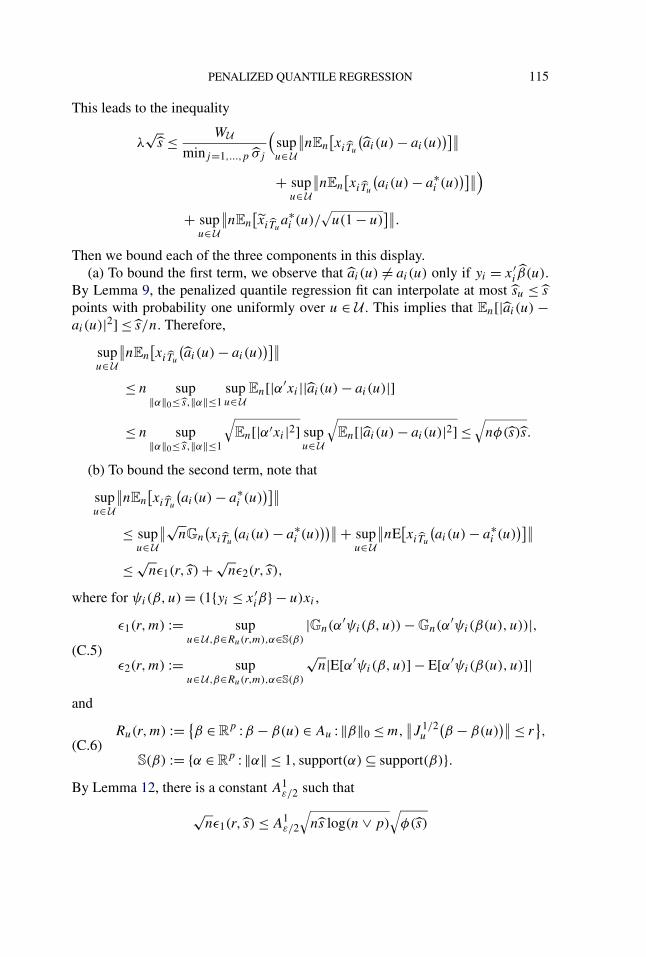
PENALIZED QUANTILE REGRESSION 115
This leads to the inequality
λ√
s ≤ WUminj=1,...,p σj
(supu∈ U
∥∥nEn
[xiTu
(ai (u) − ai(u)
)]∥∥+ sup
u∈ U
∥∥nEn
[xiTu
(ai(u) − a∗
i (u))]∥∥)
+ supu∈ U
∥∥nEn
[xiTu
a∗i (u)/
√u(1 − u)
]∥∥.Then we bound each of the three components in this display.
(a) To bound the first term, we observe that ai (u) = ai(u) only if yi = x′i β(u).
By Lemma 9, the penalized quantile regression fit can interpolate at most su ≤ s
points with probability one uniformly over u ∈ U . This implies that En[|ai(u) −ai(u)|2] ≤ s/n. Therefore,
supu∈ U
∥∥nEn
[xiTu
(ai(u) − ai(u)
)]∥∥≤ n sup
‖α‖0≤ s,‖α‖≤1supu∈ U
En[|α′xi ||ai(u) − ai(u)|]
≤ n sup‖α‖0≤ s,‖α‖≤1
√En[|α′xi |2] sup
u∈ U
√En[|ai(u) − ai(u)|2] ≤
√nφ(s)s.
(b) To bound the second term, note that
supu∈ U
∥∥nEn
[xiTu
(ai(u) − a∗
i (u))]∥∥
≤ supu∈ U
∥∥√nGn
(xiTu
(ai(u) − a∗
i (u)))∥∥+ sup
u∈ U
∥∥nE[xiTu
(ai(u) − a∗
i (u))]∥∥
≤ √nε1(r, s) + √
nε2(r, s),
where for ψi(β,u) = (1{yi ≤ x′iβ} − u)xi ,
ε1(r,m) := supu∈ U ,β∈Ru(r,m),α∈S(β)
|Gn(α′ψi(β,u)) − Gn(α
′ψi(β(u),u))|,(C.5)
ε2(r,m) := supu∈ U ,β∈Ru(r,m),α∈S(β)
√n|E[α′ψi(β,u)] − E[α′ψi(β(u),u)]|
and
Ru(r,m) := {β ∈ R
p :β − β(u) ∈ Au :‖β‖0 ≤ m,∥∥J 1/2
u
(β − β(u)
)∥∥ ≤ r},
(C.6)S(β) := {α ∈ R
p :‖α‖ ≤ 1, support(α) ⊆ support(β)}.By Lemma 12, there is a constant A1
ε/2 such that
√nε1(r, s) ≤ A1
ε/2
√ns log(n ∨ p)
√φ(s)

116 A. BELLONI AND V. CHERNOZHUKOV
with probability 1 − ε/2. By Lemma 10, we have√
nε2(r, s) ≤ n(μ(s)/2)(r ∧ 1).(c) To bound the last term, by Theorem 1 there exists a constant A0
ε/2 such thatwith probability 1 − ε/2
supu∈ U
∥∥nEn
[xiTu
a∗i (u)/
√u(1 − u)
]∥∥ ≤ √s� ≤ √
sA0ε/2WU
√n logp,
where we used that a∗i (u) = u − 1{ui ≤ u}, i = 1, . . . , n, for u1, . . . , un i.i.d. uni-
form (0,1).Combining bounds in (a)–(c), using that minj=1,...,p σj ≥ 1/2 by condition D.3
with probability 1 − γ , we have√
s
WU≤ μ(s)
n
λ(r ∧ 1) + √
sKε
√n log(n ∨ p)φ(s)
λ,
with probability at least 1 − ε − γ , for Kε = 2(1 + A0ε/2 + A1
ε/2). �
Next we control the linearization error ε2 defined in (C.5).
LEMMA 10 (Controlling linearization error ε2). Under D.1, D.2,
ε2(r,m) ≤ √n√
ϕmax(m){1 ∧ (2[f /f 1/2]r)} for all r > 0 and m ≤ n.
PROOF. By definition
ε2(r,m) = supu∈ U ,β∈Ru(r,m),α∈S(β)
√n∣∣E[(α′xi)
(1{yi ≤ x′
iβ} − 1{yi < x′iβ(u)})]∣∣.
By Cauchy–Schwarz, and using that ϕmax(m) = sup‖α‖≤1,‖α‖0≤m E[|α′xi |2],
ε2(r,m) ≤ √n√
ϕmax(m) supu∈ U ,β∈Ru(r,m)
√E[(
1{yi ≤ x′iβ} − 1{yi < x′
iβ(u)})2].
Then, since for any β ∈ Ru(r,m), u ∈ U ,
E[(
1{yi ≤ x′iβ} − 1{yi < x′
iβ(u)})2]≤ E
[1{|yi − x′
iβ(u)| ≤ ∣∣x′i
(β − β(u)
)∣∣}]≤ E
[(2f
∣∣x′i
(β − β(u)
)∣∣)∧ 1] ≤ {
2f(E[∣∣x′
i
(β − β(u)
)∣∣2])1/2}∧ 1
and (E[|x′i (β − β(u))|2])1/2 ≤ ‖J 1/2
u (β − β(u))‖/f 1/2 by Lemma 4, the resultfollows. �
Next, we proceed to control the empirical error ε1 defined in (C.5). We shallneed the following preliminary result on the uniform L2 covering numbers [33] ofa relevant function class.
PENALIZED QUANTILE REGRESSION 117
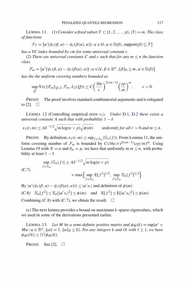
LEMMA 11. (1) Consider a fixed subset T ⊂ {1,2, . . . , p}, |T | = m. The classof functions
FT = {α′(ψi(β,u) − ψi(β(u),u)
):u ∈ U , α ∈ S(β), support(β) ⊆ T
}has a VC index bounded by cm for some universal constant c.
(2) There are universal constants C and c such that for any m ≤ n the functionclass
Fm = {α′(ψi(β,u) − ψi(β(u),u)
):u ∈ U , β ∈ R
p,‖β‖0 ≤ m,α ∈ S(β)}
has the the uniform covering numbers bounded as
supQ
N(ε‖Fm‖Q,2, Fm,L2(Q)) ≤ C
(16e
ε
)2(cm−1)(ep
m
)m
, ε > 0.
PROOF. The proof involves standard combinatorial arguments and is relegatedto [2]. �
LEMMA 12 (Controlling empirical error ε1). Under D.1, D.2 there exists auniversal constant A such that with probability 1 − δ
ε1(r,m) ≤ Aδ−1/2√
m log(n ∨ p)√
φ(m) uniformly for all r > 0 and m ≤ n.
PROOF. By definition, ε1(r,m) ≤ supf ∈Fm|Gn(f )|. From Lemma 11, the uni-
form covering number of Fm is bounded by C(16e/ε)2(cm−1)(ep/m)m. UsingLemma 19 with N = n and θm = p, we have that uniformly in m ≤ n, with proba-bility at least 1 − δ
supf ∈Fm
|Gn(f )| ≤ Aδ−1/2√
m log(n ∨ p)
(C.7)× max
{sup
f ∈Fm
E[f 2]1/2, supf∈Fm
En[f 2]1/2}.
By |α′(ψi(β,u) − ψi(β(u),u))| ≤ |α′xi | and definition of φ(m)
En[f 2] ≤ En[|α′xi |2] ≤ φ(m) and E[f 2] ≤ E[|α′xi |2] ≤ φ(m).(C.8)
Combining (C.8) with (C.7), we obtain the result. �
(c) The next lemma provides a bound on maximum k-sparse eigenvalues, whichwe used in some of the derivations presented earlier.
LEMMA 13. Let M be a semi-definite positive matrix and φM(k) = sup{α′ ×Mα :α ∈ R
p,‖α‖ = 1,‖α‖0 ≤ k}. For any integers k and �k with � ≥ 1, we haveφM(�k) ≤ ���φM(k).
PROOF. See [2]. �
118 A. BELLONI AND V. CHERNOZHUKOV
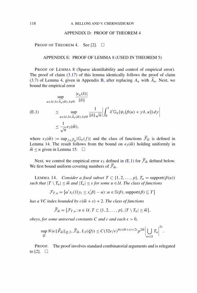
APPENDIX D: PROOF OF THEOREM 4
PROOF OF THEOREM 4. See [2]. �
APPENDIX E: PROOF OF LEMMA 8 (USED IN THEOREM 5)
PROOF OF LEMMA 8 (Sparse identifiability and control of empirical error).The proof of claim (3.17) of this lemma identically follows the proof of claim(3.7) of Lemma 4, given in Appendix B, after replacing Au with Au. Next, webound the empirical error
supu∈ U ,δ∈Au(m),δ =0
|εu(δ)|‖δ‖
≤ supu∈ U ,δ∈Au(m),δ =0
1
‖δ‖√n
∣∣∣∣∫ 1
0δ′
Gn
(ψi
(β(u) + γ δ,u
))dγ
∣∣∣∣(E.1)
≤ 1√nε3(m),
where ε3(m) := supf ∈Fm|Gn(f )| and the class of functions Fm is defined in
Lemma 14. The result follows from the bound on ε3(m) holding uniformly inm ≤ n given in Lemma 15. �
Next, we control the empirical error ε3 defined in (E.1) for Fm defined below.We first bound uniform covering numbers of Fm.
LEMMA 14. Consider a fixed subset T ⊂ {1,2, . . . , p}, Tu = support(β(u))
such that |T \ Tu| ≤ m and |Tu| ≤ s for some u ∈ U . The class of functions
FT ,u = {α′xi(1{yi ≤ x′
iβ} − u) :α ∈ S(β), support(β) ⊆ T}
has a VC index bounded by c(m + s) + 2. The class of functions
Fm = {FT ,u :u ∈ U , T ⊂ {1,2, . . . , p}, |T \ Tu| ≤ m
},
obeys, for some universal constants C and c and each ε > 0,
supQ
N(ε‖Fm‖Q,2, Fm,L2(Q)) ≤ C(32e/ε)4(c(m+s)+2)p2m
∣∣∣∣ ⋃u∈ U
Tu
∣∣∣∣2s
.
PROOF. The proof involves standard combinatorial arguments and is relegatedto [2]. �
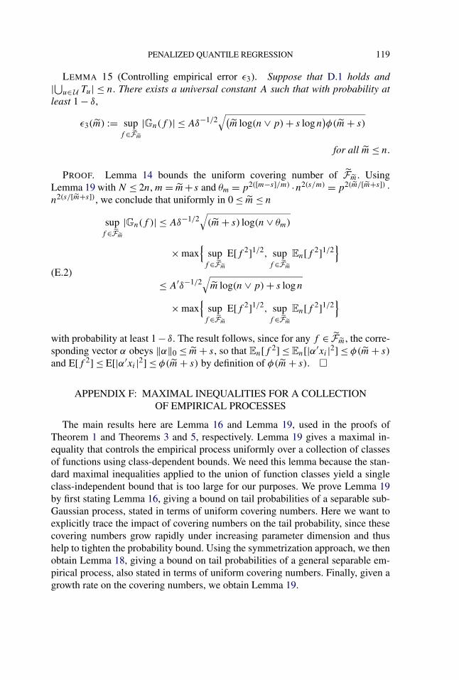
PENALIZED QUANTILE REGRESSION 119
LEMMA 15 (Controlling empirical error ε3). Suppose that D.1 holds and|⋃u∈ U Tu| ≤ n. There exists a universal constant A such that with probability atleast 1 − δ,
ε3(m) := supf ∈Fm
|Gn(f )| ≤ Aδ−1/2√(
m log(n ∨ p) + s logn)φ(m + s)
for all m ≤ n.
PROOF. Lemma 14 bounds the uniform covering number of Fm. UsingLemma 19 with N ≤ 2n, m = m+ s and θm = p2([m−s]/m) ·n2(s/m) = p2(m/[m+s]) ·n2(s/[m+s]), we conclude that uniformly in 0 ≤ m ≤ n
supf ∈Fm
|Gn(f )| ≤ Aδ−1/2√
(m + s) log(n ∨ θm)
× max{
supf ∈Fm
E[f 2]1/2, supf ∈Fm
En[f 2]1/2}
(E.2)≤ A′δ−1/2
√m log(n ∨ p) + s logn
× max{
supf ∈Fm
E[f 2]1/2, supf ∈Fm
En[f 2]1/2}
with probability at least 1 − δ. The result follows, since for any f ∈ Fm, the corre-sponding vector α obeys ‖α‖0 ≤ m + s, so that En[f 2] ≤ En[|α′xi |2] ≤ φ(m + s)
and E[f 2] ≤ E[|α′xi |2] ≤ φ(m + s) by definition of φ(m + s). �
APPENDIX F: MAXIMAL INEQUALITIES FOR A COLLECTIONOF EMPIRICAL PROCESSES
The main results here are Lemma 16 and Lemma 19, used in the proofs ofTheorem 1 and Theorems 3 and 5, respectively. Lemma 19 gives a maximal in-equality that controls the empirical process uniformly over a collection of classesof functions using class-dependent bounds. We need this lemma because the stan-dard maximal inequalities applied to the union of function classes yield a singleclass-independent bound that is too large for our purposes. We prove Lemma 19by first stating Lemma 16, giving a bound on tail probabilities of a separable sub-Gaussian process, stated in terms of uniform covering numbers. Here we want toexplicitly trace the impact of covering numbers on the tail probability, since thesecovering numbers grow rapidly under increasing parameter dimension and thushelp to tighten the probability bound. Using the symmetrization approach, we thenobtain Lemma 18, giving a bound on tail probabilities of a general separable em-pirical process, also stated in terms of uniform covering numbers. Finally, given agrowth rate on the covering numbers, we obtain Lemma 19.
120 A. BELLONI AND V. CHERNOZHUKOV
LEMMA 16 (Exponential inequality for sub-Gaussian process). Consider anylinear zero-mean separable process {G(f ) :f ∈ F }, whose index set F includeszero, is equipped with a L2(P ) norm, and has envelope F . Suppose furtherthat the process is sub-Gaussian, namely for each g ∈ F − F : P{|G(g)| > η} ≤2 exp(−1
2η2/D2‖g‖2P,2) for any η > 0, with D a positive constant; and suppose
that we have the following upper bound on the L2(P ) covering numbers for F :
N(ε‖F‖P,2, F ,L2(P )) ≤ n(ε, F ,P ) for each ε > 0,
where n(ε, F ,P ) is increasing in 1/ε, and ε√
logn(ε, F ,P ) → 0 as 1/ε → ∞and is decreasing in 1/ε. Then for K > D, for some universal constant c < 30,ρ(F ,P ) := supf ∈F ‖f ‖P,2/‖F‖P,2,
P
{ supf ∈F |G(f )|‖F‖P,2
∫ ρ(F ,P )/40
√logn(x, F ,P )dx
> cK
}
≤∫ ρ(F ,P )/2
0ε−1n(ε, F ,P )−{(K/D)2−1} dε.
The result of Lemma 16 is in spirit of the Talagrand tail inequality for Gaussianprocesses. Our result is less sharp than Talagrand’s result in the Gaussian case (bya log factor), but it applies to more general sub-Gaussian processes.
In order to prove a bound on tail probabilities of a general separable empiri-cal process, we need to go through a symmetrization argument. Since we use adata-dependent threshold, we need an appropriate extension of the classical sym-metrization lemma to allow for this. Let us call a threshold function x : Rn �→ R
k-sub-exchangeable if, for any v,w ∈ Rn and any vectors v, w created by the
pairwise exchange of the components in v with components in w, we have thatx(v) ∨ x(w) ≥ [x(v) ∨ x(w)]/k. Several functions satisfy this property, in par-ticular x(v) = ‖v‖ with k = √
2 and constant functions with k = 1. The follow-ing result generalizes the standard symmetrization lemma for probabilities (Lem-ma 2.3.7 of [33]) to the case of a random threshold x that is sub-exchangeable.
LEMMA 17 (Symmetrization with data-dependent thresholds). Consider ar-bitrary independent stochastic processes Z1, . . . ,Zn and arbitrary functionsμ1, . . . ,μn : F �→ R. Let x(Z) = x(Z1, . . . ,Zn) be a k-sub-exchangeable ran-dom variable and for any τ ∈ (0,1) let qτ denote the τ quantile of x(Z),pτ := P(x(Z) ≤ qτ ) ≥ τ and pτ := P(x(Z) < qτ ) ≤ τ . Then
P
(∥∥∥∥∥n∑
i=1
Zi
∥∥∥∥∥F
> x0 ∨ x(Z)
)≤ 4
pτ
P
(∥∥∥∥∥n∑
i=1
εi(Zi − μi)
∥∥∥∥∥F
>x0 ∨ x(Z)
4k
)+ pτ ,
where x0 is a constant such that inff ∈F P(|∑ni=1 Zi(f )| ≤ x0
2 ) ≥ 1 − pτ
2 .
PENALIZED QUANTILE REGRESSION 121
Note that we can recover the classical symmetrization lemma for fixed thresh-olds by setting k = 1, pτ = 1 and pτ = 0.
LEMMA 18 (Exponential inequality for separable empirical process). Con-sider a separable empirical process Gn(f ) = n−1/2 ∑n
i=1{f (Zi)− E[f (Zi)]} andthe empirical measure Pn for Z1, . . . ,Zn, an underlying i.i.d. data sequence. LetK > 1 and τ ∈ (0,1) be constants, and en(F ,Pn) = en(F ,Z1, . . . ,Zn) be a k-sub-exchangeable random variable, such that
‖F‖Pn,2
∫ ρ(F ,Pn)/4
0
√logn(ε, F ,Pn) dε ≤ en(F ,Pn)
and
supf ∈F
varP
f ≤ τ
2(4kcKen(F ,Pn))
2
for the same constant c > 0 as in Lemma 16, then
P
{supf ∈F
|Gn(f )| ≥ 4kcKen(F ,Pn)}
≤ 4
τEP
([∫ ρ(F ,Pn)/2
0ε−1n(ε, F ,Pn)
−{K2−1} dε
]∧ 1
)+ τ.
Finally, our main result in this section is as follows.
LEMMA 19 (Maximal inequality for a collection of empirical processes).Consider a collection of separable empirical processes
Gn(f ) = n−1/2n∑
i=1
{f (Zi) − E[f (Zi)]},
where Z1, . . . ,Zn is an underlying i.i.d. data sequence, defined over functionclasses Fm,m = 1, . . . ,N with envelopes Fm = supf ∈Fm
|f (x)|,m = 1, . . . ,N ,and with upper bounds on the uniform covering numbers of Fm given for all m
by
n(ε, Fm,Pn) = (N ∨ n ∨ θm)m(ω/ε)υm, 0 < ε < 1,
with some constants ω > 1, υ > 1 and θm ≥ θ0. For a constant C := (1 + √2υ)/4
set
en(Fm,Pn) = C√
m log(N ∨ n ∨ θm ∨ ω)max{
supf ∈Fm
‖f ‖P,2, supf ∈Fm
‖f ‖Pn,2
}.
Then, for any δ ∈ (0,1/6), and any constant K ≥ √2/δ we have
supf ∈Fm
|Gn(f )| ≤ 4√
2cKen(Fm,Pn) for all m ≤ N,
with probability at least 1 − δ, provided that N ∨ n ∨ θ0 ≥ 3; the constant c is thesame as in Lemma 16.
122 A. BELLONI AND V. CHERNOZHUKOV
PROOF OF LEMMA 16. The strategy of the proof is similar to the proof ofLemma 19.34 in [31], page 286, given for the expectation of a supremum of aprocess; here we instead bound tail probabilities and also compute all constantsexplicitly.
Step 1. There exists a sequence of nested partitions of F , {(Fqi, i = 1, . . . ,Nq),q = q0, q0 +1, . . .} where the qth partition consists of sets of L2(P ) radius at most‖F‖P,22−q , and q0 is the largest positive integer such that 2−q0 ≤ ρ(F ,P )/4 sothat q0 ≥ 2. The existence of such a partition follows from a standard argument,for example, [31], page 286.
Let fqi be an arbitrary point of Fqi . Set πq(f ) = fqi if f ∈ Fqi . By sep-arability of the process, we can replace F by
⋃q,i fqi , since the supremum
norm of the process can be computed by taking this set only. In this case, wecan decompose f − πq0(f ) = ∑∞
q=q0+1(πq(f ) − πq−1(f )). Hence by linearityG(f ) − G(πq0(f )) = ∑∞
q=q0+1 G(πq(f ) − πq−1(f )), so that
P
{supf ∈F
|G(f )| >∞∑
q=q0
ηq
}≤
∞∑q=q0+1
P
{max
f
∣∣G(πq(f ) − πq−1(f )
)∣∣ > ηq
}+ P
{max
f|G(πq0(f ))| > ηq0
},
for constants ηq chosen below.Step 2. By construction of the partition sets ‖πq(f ) − πq−1(f )‖P,2 ≤ 2 ×
‖F‖P,22−(q−1) ≤ 4‖F‖P,22−q , for q ≥ q0 + 1. Setting ηq = 8K‖F‖P,22−q ×√logNq, using sub-Gaussianity, setting K > D, using that 2 logNq ≥ logNq ×
Nq−1 ≥ lognq , using that q �→ lognq is increasing in q , and 2−q0 ≤ ρ(F ,P )/4,we obtain
∞∑q=q0+1
P
{max
f
∣∣G(πq(f ) − πq−1(f )
)∣∣ > ηq
}
≤∞∑
q=q0+1
NqNq−12 exp(−η2
q/(4D‖F‖P,22−q)2)
≤∞∑
q=q0+1
NqNq−12 exp(−(K/D)22 logNq
)
≤∞∑
q=q0+1
2 exp(−{(K/D)2 − 1} lognq
)≤∫ ∞q0
2 exp(−{(K/D)2 − 1} lognq
)dq
=∫ ρ(F ,P )/4
0(x ln 2)−12n(x, F ,P )−{(K/D)2−1} dx.
PENALIZED QUANTILE REGRESSION 123
By Jensen’s inequality, we have√
logNq ≤ aq := ∑qj=q0
√lognj , so that we
obtain∑∞
q=q0+1 ηq ≤ 8∑∞
q=q0+1 K‖F‖P,22−qaq . Letting bq = 2 · 2−q , noting
aq+1 − aq =√
lognq+1 and bq+1 − bq = −2−q , we get using summation by parts
∞∑q=q0+1
2−qaq = −∞∑
q=q0+1
(bq+1 − bq)aq
= −aqbq |∞q0+1 +∞∑
q=q0+1
bq+1(aq+1 − aq)
= 2 · 2−(q0+1)√
lognq0+1 +∞∑
q=q0+1
2 · 2−(q+1)√
lognq+1
= 2∞∑
q=q0+1
2−q√
lognq,
where we use the assumption that 2−q√
lognq → 0 as q → ∞, so that
−aqbq |∞q0+1 = 2 · 2−(q0+1)√
lognq0+1.
Using that 2−q√
lognq is decreasing in q by assumption,
2∞∑
q=q0+1
2−q√
lognq ≤ 2∫ ∞q0
2−q√
logn(2−q, F ,P )dq.
Using a change of variables and that 2−q0 ≤ ρ(F ,P )/4, we finally conclude that
∞∑q=q0+1
ηq ≤ K‖F‖P,216
log 2
∫ ρ(F ,P )/4
0
√logn(x, F ,P )dx.
Step 3. Letting ηq0 = K‖F‖P,2ρ(F ,P )√
2 logNq0 , recalling that Nq0 = nq0 ,using that ‖πq0(f )‖P,2 ≤ ‖F‖P,2 and sub-Gaussianity, we conclude
P
{max
f|G(πq0(f ))| > ηq0
}≤ nq2 exp
(−(K/D)2 lognq
) ≤ 2 exp(−{(K/D)2 − 1} lognq
)≤∫ q0
q0−12 exp
(−{(K/D)2 − 1} lognq
)dq
=∫ ρ(F ,P )/2
ρ(F ,P )/4(x ln 2)−12n(x, F ,P )−{(K/D)2−1} dx.
124 A. BELLONI AND V. CHERNOZHUKOV
Also, since nq0 = n(2−q0, F ,P ), 2−q0 ≤ ρ(F ,P )/4 and n(x, F ,P ) is increasing
in 1/x, we obtain ηq0 ≤ 4√
2K‖F‖P,2∫ ρ(F ,P )/4
0√
logn(x, F ,P )dx.Step 4. Finally, adding the bounds on tail probabilities from Steps 2 and 3
we obtain the tail bound stated in the main text. Further, adding bounds on ηq
from Steps 2 and 3, and using c = 16/log 2 + 4√
2 < 30, we obtain∑∞
q=q0ηq ≤
cK‖F‖P,2∫ ρ(F ,P )/4
0√
logn(x, F ,P )dx. �
PROOF OF LEMMA 17. The proof proceeds analogously to the proof ofLemma 2.3.7 (page 112) in [33] with the necessary adjustments. Letting qτ bethe τ quantile of x(Z) we have
P
{∥∥∥∥∥n∑
i=1
Zi
∥∥∥∥∥F
> x0 ∨ x(Z)
}≤ P
{x(Z) ≥ qτ ,
∥∥∥∥∥n∑
i=1
Zi
∥∥∥∥∥F
> x0 ∨ x(Z)
}+ P {x(Z) < qτ }.
Next we bound the first term of the expression above. Let Y = (Y1, . . . , Yn) be anindependent copy of Z = (Z1, . . . ,Zn), suitably defined on a product space. Fixa realization of Z such that x(Z) ≥ qτ and ‖∑n
i=1 Zi‖F > x0 ∨ x(Z). Therefore,∃fZ ∈ F such that |∑n
i=1 Zi(fZ)| > x0 ∨x(Z). Conditional on such a Z and usingthe triangular inequality, we have that
PY
{x(Y ) ≤ qτ ,
∣∣∣∣∣n∑
i=1
Yi(fZ)
∣∣∣∣∣ ≤ x0
2
}
≤ PY
{∣∣∣∣∣n∑
i=1
(Yi − Zi)(fZ)
∣∣∣∣∣ > x0 ∨ x(Z) ∨ x(Y )
2
}
≤ PY
{∥∥∥∥∥n∑
i=1
(Yi − Zi)
∥∥∥∥∥F
>x0 ∨ x(Z) ∨ x(Y )
2
}.
By definition of x0, we have inff ∈F P {|∑ni=1 Yi(f )| ≤ x0
2 } ≥ 1 − pτ /2. SincePY {x(Y ) ≤ qτ } = pτ , by Bonferroni inequality we have that the left-hand sideis bounded from below by pτ − pτ /2 = pτ /2. Therefore, over the set {Z :x(Z) ≥qτ ,‖∑n
i=1 Zi‖F > x0 ∨ x(Z)} we have
pτ
2≤ PY
{∥∥∥∥∥n∑
i=1
(Yi − Zi)
∥∥∥∥∥F
>x0 ∨ x(Z) ∨ x(Y )
2
}.
Integrating over Z, we obtain
pτ
2P
{x(Z) ≥ qτ ,
∥∥∥∥∥n∑
i=1
Zi
∥∥∥∥∥F
> x0 ∨ x(Z)
}
≤ PZPY
{∥∥∥∥∥n∑
i=1
(Yi − Zi)
∥∥∥∥∥F
>x0 ∨ x(Z) ∨ x(Y )
2
}.
PENALIZED QUANTILE REGRESSION 125
Let ε1, . . . , εn be an independent sequence of Rademacher random variables.Given ε1, . . . , εn, set (Yi = Yi, Zi = Zi) if εi = 1 and (Yi = Zi, Zi = Yi) ifεi = −1. That is, we create vectors Y and Z by pairwise exchanging their compo-nents; by construction, conditional on each ε1, . . . , εn, (Y , Z) has the same distri-bution as (Y,Z). Therefore,
PZPY
{∥∥∥∥∥n∑
i=1
(Yi − Zi)
∥∥∥∥∥F
>x0 ∨ x(Z) ∨ x(Y )
2
}
= EεPZPY
{∥∥∥∥∥n∑
i=1
(Yi − Zi)
∥∥∥∥∥F
>x0 ∨ x(Z) ∨ x(Y )
2
}.
By x(·) being k-sub-exchangeable, and since εi(Yi − Zi) = (Yi − Zi), we havethat
EεPZPY
{∥∥∥∥∥n∑
i=1
(Yi − Zi)
∥∥∥∥∥F
>x0 ∨ x(Z) ∨ x(Y )
2
}
≤ EεPZPY
{∥∥∥∥∥n∑
i=1
εi(Yi − Zi)
∥∥∥∥∥F
>x0 ∨ x(Z) ∨ x(Y )
2k
}.
By the triangular inequality and removing x(Y ) or x(Z), the latter is bounded by
P
{∥∥∥∥∥n∑
i=1
εi(Yi − μi)
∥∥∥∥∥F
>x0 ∨ x(Y )
4k
}
+ P
{∥∥∥∥∥n∑
i=1
εi(Zi − μi)
∥∥∥∥∥F
>x0 ∨ x(Z)
4k
}.
�
PROOF OF LEMMA 18. Let Gon(f ) = n−1/2 ∑n
i=1{εif (Zi)} be the sym-metrized empirical process, where ε1, . . . , εn are i.i.d. Rademacher randomvariables, that is, P(εi = 1) = P(εi = −1) = 1/2, which are independent ofZ1, . . . ,Zn. By the Chebyshev’s inequality and the assumption on en(F ,Pn), wehave for the constant τ fixed in the statement of the lemma
P(|Gn(f )| > 4kcKen(F ,Pn)
) ≤ supf varP Gn(f )
(4kcKen(F ,Pn))2 = supf ∈F varP f
(4kcKen(F ,Pn))2
≤ τ/2.
Therefore, by the symmetrization Lemma 17, we obtain
P
{supf ∈F
|Gn(f )| > 4kcKen(F ,Pn)}
≤ 4
τP
{supf ∈F
|Gon(f )| > cKen(F ,Pn)
}+ τ.
We then condition on the values of Z1, . . . ,Zn, denoting the conditional prob-ability measure as Pε . Conditional on Z1, . . . ,Zn, by the Hoeffding inequality
126 A. BELLONI AND V. CHERNOZHUKOV
the symmetrized process Gon is sub-Gaussian for the L2(Pn) norm, namely, for
g ∈ F − F , Pε{Gon(g) > x} ≤ 2 exp(−x2/[2‖g‖2
Pn,2]). Hence, by Lemma 16 withD = 1, we can bound
Pε
{supf ∈F
|Gon(f )| ≥ cKen(F ,Pn)
}≤[∫ ρ(F ,Pn)/2
0ε−1n(ε, F ,P )−{K2−1} dε
]∧ 1.
The result follows from taking the expectation over Z1, . . . ,Zn. �
PROOF OF LEMMA 19. Step 1 (Main step). In this step, we prove the main re-sult. First, we observe that the bound ε �→ n(ε, Fm,Pn) satisfies the monotonicityhypotheses of Lemma 18 uniformly in m ≤ N .
Second, recall en(Fm,Pn) := C√
m log(N ∨ n ∨ θm ∨ ω)max{supf ∈Fm‖f ‖P,2,
supf ∈Fm‖f ‖Pn,2} for C = (1 + √
2υ)/4. Note that supf ∈Fm‖f ‖Pn,2 is
√2-sub-
exchangeable and ρ(Fm,Pn) := supf ∈Fm‖f ‖Pn,2/‖Fm‖Pn,2 ≥ 1/
√n by Step 2
below. Thus, uniformly in m ≤ N ,
‖Fm‖Pn,2
∫ ρ(Fm,Pn)/4
0
√logn(ε, Fm,Pn) dε
≤ ‖Fm‖Pn,2
∫ ρ(Fm,Pn)/4
0
√m log(N ∨ n ∨ θm) + υm log(ω/ε) dε
≤ (1/4)√
m log(N ∨ n ∨ θm) supf ∈Fm
‖f ‖Pn,2
+ ‖Fm‖Pn,2
∫ ρ(Fm,Pn)/4
0
√υm log(ω/ε) dε
≤√
m log(N ∨ n ∨ θm ∨ ω) supf ∈Fm
‖f ‖Pn,2(1 + √
2υ)/4
≤ en(Fm,Pn),
which follows by
∫ ρ
0
√log(ω/ε) dε ≤
(∫ ρ
01dε
)1/2(∫ ρ
0log(ω/ε) dε
)1/2
≤ ρ√
2 log(n ∨ ω) for 1/√
n ≤ ρ ≤ 1.
Third, for any K ≥ √2/δ > 1 we have (K2 − 1) ≥ 1/δ, and let τm = δ/
(4m log(N ∨ n ∨ θ0)). Recall that 4√
2cC > 4 where 4 < c < 30 is defined inLemma 16. Note that for any m ≤ N and f ∈ Fm, we have by Chebyshev’s in-
PENALIZED QUANTILE REGRESSION 127
equality
P(|Gn(f )| > 4
√2cKen(Fm,Pn)
) ≤ supf ∈Fm‖f ‖2
P,2
(4√
2cKen(Fm,Pn))2
≤ δ/2
(4√
2cC)2m log(N ∨ n ∨ θ0)
≤ τm/2.
By Lemma 18 with our choice of τm, m ≤ N , ω > 1, υ > 1 and ρ(Fm,Pn) ≤ 1,
P
{sup
f ∈Fm
|Gn(f )| > 4√
2cKen(Fm,Pn),∃m ≤ N}
≤N∑
m=1
P
{sup
f ∈Fm
|Gn(f )| > 4√
2cKen(Fm,Pn)}
≤N∑
m=1
[4(N ∨ n ∨ θm)−m/δ
τm
∫ 1/2
0(ω/ε)(−υm/δ)+1 dε + τm
]
≤ 4N∑
m=1
(N ∨ n ∨ θm)−m/δ
τm
1
υm/δ+
N∑m=1
τm
< 16(N ∨ n ∨ θ0)
−1/δ
1 − (N ∨ n ∨ θ0)−1/δlog(N ∨ n ∨ θ0) + δ
4
(1 + logN)
log(N ∨ n ∨ θ0)≤ δ,
where the last inequality follows by N ∨ n ∨ θ0 ≥ 3 and δ ∈ (0,1/6).Step 2 (Auxiliary calculations). To establish that supf ∈Fm
‖f ‖Pn,2 is√
2-sub-exchangeable, let Z and Y be created by exchanging any components in Z withcorresponding components in Y . Then
√2(
supf ∈Fm
‖f ‖Pn(Z),2 ∨ sup
f ∈Fm
‖f ‖Pn(Y ),2
)≥(
supf ∈Fm
‖f ‖2Pn(Z),2 + sup
f ∈Fm
‖f ‖2Pn(Y ),2
)1/2
≥(
supf ∈Fm
En[f (Zi)2] + En[f (Yi)
2])1/2
=(
supf ∈Fm
En[f (Zi)2] + En[f (Yi)
2])1/2
≥(
supf ∈Fm
‖f ‖2Pn(Z),2 ∨ sup
f ∈Fm
‖f ‖2Pn(Y ),2
)1/2
= supf ∈Fm
‖f ‖Pn(Z),2 ∨ supf ∈Fm
‖f ‖Pn(Y ),2.
128 A. BELLONI AND V. CHERNOZHUKOV
Next we show that ρ(Fm,Pn) := supf ∈Fm‖f ‖Pn,2/‖Fm‖Pn,2 ≥ 1/
√n for
m ≤ N . The latter bound follows from En[F 2m] = En[supf ∈Fm
|f (Zi)|2] ≤supi≤n supf ∈Fm
|f (Zi)|2, and from
supf ∈Fm
En[|f (Zi)|2] ≥ supf ∈Fm
supi≤n
|f (Zi)|2/n. �
Acknowledgments. We would like to thank Arun Chandrasekhar, DenisChetverikov, Moshe Cohen, Brigham Fradsen, Joonhwan Lee, Ye Luo and Pierre-Andre Maugis for thorough proofreading of several versions of this paper and theirdetailed comments that helped us considerably improve the paper. We also wouldlike to thank Don Andrews, Alexandre Tsybakov, the editor Susan Murphy, the As-sociate Editor and three anonymous referees for their comments that also helpedus considerably improve the paper. We would also like to thank the participantsof seminars in Brown University, CEMMAP Quantile Regression conference atUCL, Columbia University, Cowles Foundation Lecture at the Econometric Soci-ety Summer Meeting, Harvard-MIT, Latin American Meeting 2008 of the Econo-metric Society, Winter 2007 North American Meeting of the Econometric Society,London Business School, PUC-Rio, the Stats in the Chateau, the Triangle Econo-metrics Conference and University College London.
SUPPLEMENTARY MATERIAL
Supplement to “�1-penalized quantile regression in high-dimensionalsparse models” (DOI: 10.1214/10-AOS827SUPP; .pdf). We included technicalproofs omitted from the main text: Examples of simple sufficient conditions, VCindex bounds and Gaussian sparse eigenvalues.
REFERENCES
[1] BELLONI, A. and CHERNOZHUKOV, V. (2009). Computational complexity of MCMC-basedestimators in large samples. Ann. Statist. 37 2011–2055. MR2533478
[2] BELLONI, A. and CHERNOZHUKOV, V. (2010). Supplement to “�1-penalized quantile regres-sion in high-dimensional sparse models.” DOI: 10.1214/10-AOS827SUPP.
[3] BELLONI, A. and CHERNOZHUKOV, V. (2009). �1-penalized quantile regression in high-dimensional sparse models. Available at arXiv:0904.2931.
[4] BELLONI, A. and CHERNOZHUKOV, V. (2008). Conditional quantile processes under increas-ing dimension. Technical report, Duke and MIT.
[5] BELLONI, A. and CHERNOZHUKOV, V. (2009). Post-�1-penalized estimators in high-dimensional linear regression models. Available at arXiv:1001.0188.
[6] BERTSIMAS, D. and TSITSIKLIS, J. (1997). Introduction to Linear Optimization. Athena Sci-entific, Belmont, MA.
[7] BICKEL, P. J., RITOV, Y. and TSYBAKOV, A. B. (2009). Simultaneous analysis of Lasso andDantzig selector. Ann. Statist. 37 1705–1732. MR2533469
[8] BUCHINSKY, M. (1994). Changes in the U.S. wage structure 1963–1987: Application of quan-tile regression. Econometrica 62 405–458.
PENALIZED QUANTILE REGRESSION 129
[9] BUNEA, F., TSYBAKOV, A. B. and WEGKAMP, M. H. (2006). Aggregation and sparsity via �1penalized least squares. In Proceedings of 19th Annual Conference on Learning Theory(COLT 2006) (G. Lugosi and H. U. Simon, eds.). Lecture Notes in Artificial Intelligence4005 379–391. Springer, Berlin. MR2280619
[10] BUNEA, F., TSYBAKOV, A. B. and WEGKAMP, M. H. (2007). Aggregation for Gaussian re-gression. Ann. Statist. 35 1674–1697. MR2351101
[11] BUNEA, F., TSYBAKOV, A. and WEGKAMP, M. H. (2007). Sparsity oracle inequalities for theLasso. Electron. J. Stat. 1 169–194. MR2312149
[12] CANDES, E. and TAO, T. (2007). The Dantzig selector: Statistical estimation when p is muchlarger than n. Ann. Statist. 35 2313–2351. MR2382644
[13] CHERNOZHUKOV, V. (2005). Extremal quantile regression. Ann. Statist. 33 806–839.MR2163160
[14] FAN, J. and LV, J. (2008). Sure independence screening for ultra-high dimensional featurespace. J. R. Stat. Soc. Ser. B Stat. Methodol. 70 849–911. MR2530322
[15] GUTENBRUNNER, C. and JURECKOVÁ, J. (1992). Regression rank scores and regression quan-tiles. Ann. Statist. 20 305–330. MR1150346
[16] HE, X. and SHAO, Q.-M. (2000). On parameters of increasing dimenions. J. MultivariateAnal. 73 120–135. MR1766124
[17] KNIGHT, K. (1998). Limiting distributions for L1 regression estimators under general condi-tions. Ann. Statist. 26 755–770. MR1626024
[18] KNIGHT, K. and FU, W. J. (2000). Asymptotics for Lasso-type estimators. Ann. Statist. 281356–1378. MR1805787
[19] KOENKER, R. (2005). Quantile Regression. Cambridge Univ. Press, Cambridge. MR2268657[20] KOENKER, R. (2010). Additive models for quantile regression: Model selection and confi-
dence bandaids. Working paper. Available at http://www.econ.uiuc.edu/~roger/research/bandaids/bandaids.pdf.
[21] KOENKER, R. and BASSET, G. (1978). Regression quantiles. Econometrica 46 33–50.MR0474644
[22] KOLTCHINSKII, V. (2009). Sparsity in penalized empirical risk minimization. Ann. Inst. H.Poincaré Probab. Statist. 45 7–57. MR2500227
[23] LAPLACE, P.-S. (1818). Théorie Analytique des Probabilités. Éditions Jacques Gabay (1995),Paris.
[24] LEDOUX, M. and TALAGRAND, M. (1991). Probability in Banach Spaces: Isoperimetryand Processes. Ergebnisse der Mathematik und ihrer Grenzgebiete 23. Springer, Berlin.MR1102015
[25] LOUNICI, K., PONTIL, M., TSYBAKOV, A. B. and VAN DE GEER, S. A. (2009). Takingadvantage of sparsity in multi-task learning. In COLT’09. Omnipress, Madison, WI.
[26] MEINSHAUSEN, N. and YU, B. (2009). Lasso-type recovery of sparse representations for high-dimensional data. Ann. Statist. 37 246–270. MR2488351
[27] PORTNOY, S. (1991). Asymptotic behavior of regression quantiles in nonstationary, dependentcases. J. Multivariate Anal. 38 100–113. MR1128939
[28] PORTNOY, S. and KOENKER, R. (1997). The Gaussian hare and the Laplacian tortoise: Com-putability of squared-error versus absolute-error estimators. Statist. Sci. 12 279–300.MR1619189
[29] ROSENBAUM, M. and TSYBAKOV, A. B. (2010). Sparse recovery under matrix uncertainty.Ann. Statist. 38 2620–2651.
[30] TIBSHIRANI, R. (1996). Regression shrinkage and selection via the Lasso. J. Roy. Statist. Soc.Ser. B 58 267–288. MR1379242
[31] VAN DER VAART, A. W. (1998). Asymptotic Statistics. Cambridge Univ. Press, Cambridge,MA.

130 A. BELLONI AND V. CHERNOZHUKOV
[32] VAN DE GEER, S. A. (2008). High-dimensional generalized linear models and the Lasso. Ann.Statist. 36 614–645. MR2396809
[33] VAN DER VAART, A. W. and WELLNER, J. A. (1996). Weak Convergence and EmpiricalProcesses. Springer, New York. MR1385671
[34] ZHANG, C.-H. and HUANG, J. (2008). The sparsity and bias of the Lasso selection in high-dimensional linear regression. Ann. Statist. 36 1567–1594. MR2435448
FUQUA SCHOOL OF BUSINESS
DUKE UNIVERSITY
1 TOWERVIEW DRIVE
DURHAM, NORTH CAROLINA 27708-0120PO BOX 90120USAE-MAIL: [email protected]
DEPARTMENT OF ECONOMICS
AND OPERATIONS RESEARCH CENTER
MASSACHUSETTS INSTITUTE OF TECHNOLOGY
50 MEMORIAL DRIVE
ROOM E52-262F
CAMBRIDGE, MASSACHUSETTS 02142USAE-MAIL: [email protected]

![-PENALIZED QUANTILE REGRESSION IN HIGH-DIMENSIONAL … · arXiv:0904.2931v5 [math.ST] 26 Sep 2019 ℓ1-PENALIZED QUANTILE REGRESSION IN HIGH-DIMENSIONAL SPARSE MODELS By Alexandre](https://img.pdfslide.us/doc/110x75/600b004232c44863d03e03e1/penalized-quantile-regression-in-high-dimensional-arxiv09042931v5-mathst-26.jpg)