Embed Size (px)
Citation preview

L. Vandenberghe EE133A (Spring 2016)
9. Least squares applications
• model fitting
• multiobjective least squares
• control
• estimation
• statistics
9-1

Model fitting
suppose a scalar quantity y and an n-vector x are related as
y ≈ f(x)
• y is the outcome, or response variable, or dependent variable
• x is vector of independent variables or explanatory variables
• we don’t know f , but have some idea about its general form
Model fitting
• find an approximate model f : Rn → R for f , based on observations
• we use the notation y for the model prediction of the outcome y:
y = f(x)
Least squares applications 9-2

Prediction error
we have N data points
(x1, y1), (x1, y1), . . . , (xN , yN) (with each xi ∈ Rn, yi ∈ R)
data points are also called observations, examples, samples, measurements
• model prediction for sample i is yi = f(xi)
• the prediction error or residual for sample i is
ri = yi − yi = yi − f(xi)
• the model f fits the data well if the N residuals ri are small
Least squares applications 9-3

Linearly parameterized model
suppose we choose f from a linearly parameterized family of models
f(x) = θ1f1(x) + θ2f2(x) + · · ·+ θpfp(x)
• functions fi : Rn → R are basis functions (chosen by us)
• coefficients θ1, . . . , θp are estimated model parameters
• vector of residuals r = (r1, . . . , rN) is affine in the parameters θ:
r1r2...rN
=
y1y2...yN
−
f1(x1) f2(x1) · · · fp(x1)f1(x2) f2(x2) · · · fp(x2)...
......
f1(xN) f2(xN) · · · fp(xN)
θ1θ2...
θp
Least squares applications 9-4

Least squares model fitting
select model parameters θ by minimizing the mean square error (MSE)
1
N(r21 + r22 + · · ·+ r2N) =
1
N‖r‖2
this is a linear least squares problem: θ is the solution of
minimize ‖Aθ − y‖2
with variable θ and
A =
f1(x1) f2(x1) · · · fp(x1)f1(x2) f2(x2) · · · fp(x2)...
......
f1(xN) f2(xN) · · · fp(xN)
, θ =
θ1θ2...θp
, y =
y1y2...yN
Least squares applications 9-5

Generalization and validation
Generalization ability: ability of model to predict outcomes for new data
Model validation: to assess generalization ability,
• divide data in two sets: training set and test (or validation) set
• use training set to fit model
• use test set to get an idea of generalization ability
Over-fit model
• model with low prediction error on training set, bad generalization ability
• prediction error on training set is much smaller than on test set
Least squares applications 9-6
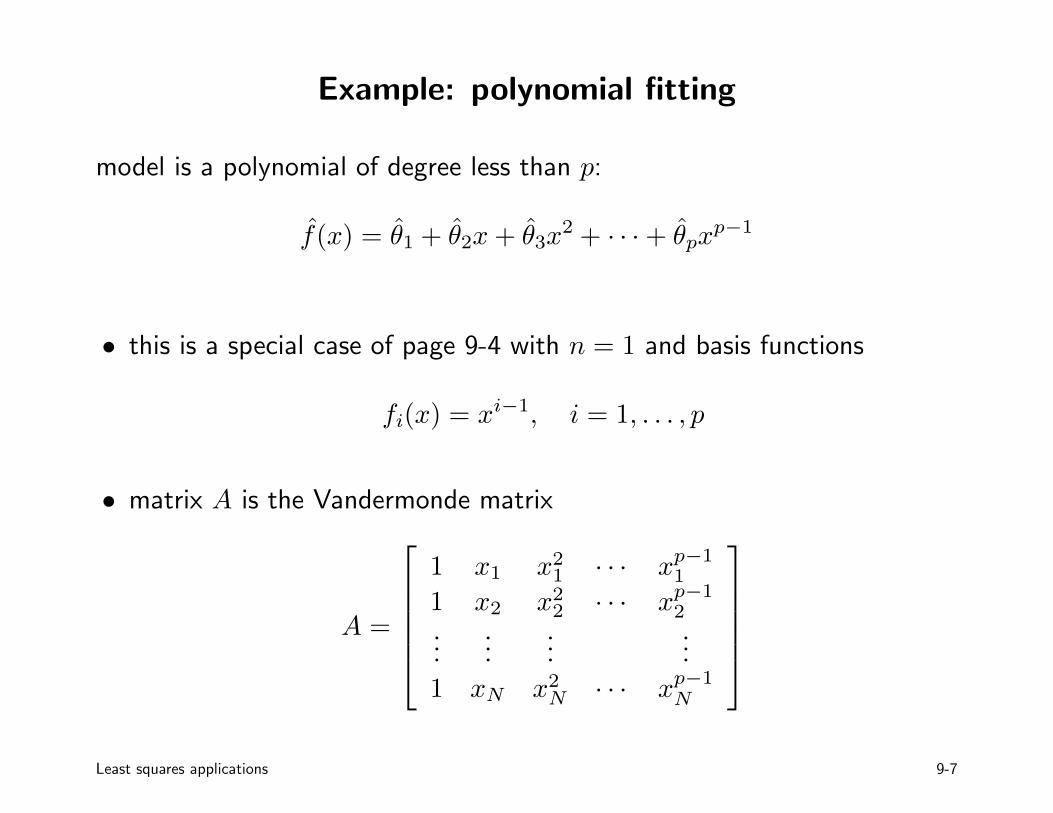
Example: polynomial fitting
model is a polynomial of degree less than p:
f(x) = θ1 + θ2x+ θ3x2 + · · ·+ θpx
p−1
• this is a special case of page 9-4 with n = 1 and basis functions
fi(x) = xi−1, i = 1, . . . , p
• matrix A is the Vandermonde matrix
A =
1 x1 x21 · · · xp−11
1 x2 x22 · · · xp−12...
......
...
1 xN x2N · · · xp−1N
Least squares applications 9-7

Example
p = 3 p = 7
p = 12 p = 20
Least squares applications 9-8
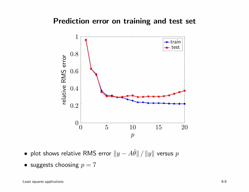
Prediction error on training and test set
0 5 10 15 200
0.2
0.4
0.6
0.8
1
p
rela
tive
RM
Ser
ror
traintest
• plot shows relative RMS error ‖y −Aθ‖ / ‖y‖ versus p
• suggests choosing p = 7
Least squares applications 9-9

Overfitting
polynomial of degree 19 (p = 20) on training and test set
training set test set
over-fitting is evident at the left end of the interval
Least squares applications 9-10

Outline
• model fitting
• multiobjective least squares
• control
• estimation
• statistics
Weighted least squares problem
find x that minimizes
λ1‖A1x− b1‖2 + λ2‖A2x− b2‖2 + · · ·+ λk‖Akx− bk‖2
• matrix Ai has size mi × n; vector bi has length mi
• coefficients λi are positive weights
• goal is to find one x that makes the k objectives ‖Aix− bi‖2 small
• in general, there is a trade-off between the k objectives
• weights λi express relative importance of different objectives
• without loss of generality, can choose λ1 = 1
Least squares applications 9-11

Solution of weighted least squares
• weighted least squares is equivalent to a standard least squares problem
minimize
∥∥∥∥∥∥∥∥∥
√λ1A1√λ2A2
...√λkAk
x−√λ1b1√λ2b2...√λkbk
∥∥∥∥∥∥∥∥∥2
• solution is unique if stacked matrix has linearly independent columns
• each matrix Ai may have linearly dependent columns (or be wide)
• solution satisfies normal equations(λ1A
T1A1 + · · ·+ λkA
TkAk
)x = λ1A
T1 b1 + · · ·+ λkA
Tk bk
Least squares applications 9-12

Example
minimize ‖A1x− b1‖2 + λ‖A2x− b2‖2
10−5 100 105
2
2.5
3
3.5
4
λ
‖A1xλ − b1‖‖A2xλ − b2‖
2.5 3 3.5 41.5
2
2.5
3
3.5
4
‖A1xλ − b1‖
‖A2xλ−b 2‖
xλ is solution of weighted least squares problem with weight λ
Least squares applications 9-13

Outline
• model fitting
• multiobjective least squares
• control
• estimation
• statistics

Control
y = Ax+ b
• x is n-vector of actions or inputs
• y is m-vector of results or outputs
• relation between inputs and outputs is known affine function
goal is to choose inputs to optimize different objectives on x and y
Least squares applications 9-14

Optimal input design
Linear dynamical system
y(t) = h0u(t) + h1u(t− 1) + h2u(t− 2) + · · ·+ htu(0)
• output y(t) and input u(t) are scalar
• we assume input u(t) is zero for t < 0
• output is linear combination of current and previous inputs
• coefficients h0, h1, . . . are the impulse response coefficients
Optimal input design
• optimization variable is the input sequence x = (u(0), u(1), . . . , u(N))
• goal is to track a desired output using a small and slowly varying input
Least squares applications 9-15
Input design objectives
minimize Jt(x) + λvJv(x) + λmJm(x)
• track desired output ydes over an interval [0, N ]:
Jt(x) =
N∑t=0
(y(t)− ydes(t))2
• use a small and slowly varying input signal:
Jm(x) =
N∑t=0
u(t)2, Jv(x) =
N−1∑t=0
(u(t+ 1)− u(t))2
Least squares applications 9-16

Tracking error
Jt(x) =
N∑t=0
(y(t)− ydes(t))2
= ‖Atx− bt‖2
with
At =
h0 0 0 · · · 0 0h1 h0 0 · · · 0 0h2 h1 h0 · · · 0 0...
......
. . ....
...hN−1 hN−2 hN−3 · · · h0 0hN hN−1 hN−2 · · · h1 h0
, bt =
ydes(0)ydes(1)ydes(2)
...ydes(N − 1)ydes(N)
Least squares applications 9-17

Input variation and magnitude
Input variation
Jv(x) =
N−1∑t=0
(u(t+ 1)− u(t))2 = ‖Dx‖2
with D the N × (N + 1) matrix
D =
−1 1 0 · · · 0 0 00 −1 1 · · · 0 0 0...
......
......
...0 0 0 · · · −1 1 00 0 0 · · · 0 −1 1
Input magnitude
Jm(x) =
N∑t=0
u(t)2 = ‖x‖2
Least squares applications 9-18

Example
λv = 0,small λm
0 50 100 150 200−6
−4
−2
0
2
4
t
u(t)
0 50 100 150 200
−1
0
1
t
y(t)
larger λv
0 50 100 150 200−6
−4
−2
0
2
4
t
u(t)
0 50 100 150 200
−1
0
1
t
y(t)
Least squares applications 9-19

Outline
• model fitting
• multiobjective least squares
• control
• estimation
• statistics

Estimation
Linear measurement model
y = Ax+ v
• n-vector x contains parameters that we want to estimate
• m-vector v is unknown measurement error or noise
• m-vector y contains measurements
• m× n matrix A relates measurements and parameters
Least squares estimate: use as estimate of x the solution x of
minimize ‖Ax− y‖2
Least squares applications 9-20

Regularized estimation
add other terms to ‖Ax− y‖2 to include information about parameters
Example: Tikhonov regularization
minimize ‖Ax− y‖2 + λ‖x‖2
• goal is to make ‖Ax− y‖ small with small x
• equivalent to solving (ATA+ λI)x = ATy
• solution is unique (if λ > 0) even when A has dependent columns
Least squares applications 9-21

Signal denoising
• observed signal is n-vector
y = x+ v
• x is unknown signal
• v is noise
0 500 1000
0.5
1
1.5
kyk
Least squares denoising
minimize ‖x− y‖2 + λ
n−1∑i=1
(xi − xi−1)2
goal is to find slowly varying signal x, close to observed signal y
Least squares applications 9-22
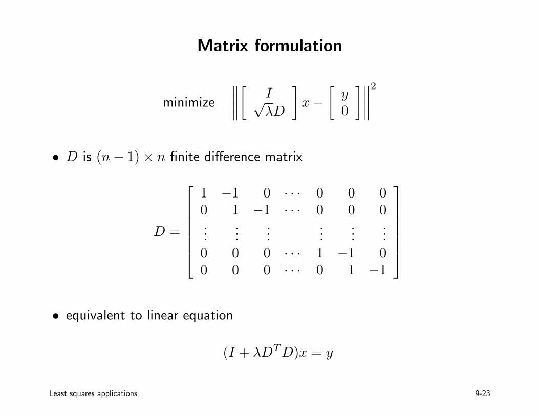
Matrix formulation
minimize
∥∥∥∥[ I√λD
]x−
[y0
]∥∥∥∥2
• D is (n− 1)× n finite difference matrix
D =
1 −1 0 · · · 0 0 00 1 −1 · · · 0 0 0...
......
......
...0 0 0 · · · 1 −1 00 0 0 · · · 0 1 −1
• equivalent to linear equation
(I + λDTD)x = y
Least squares applications 9-23

Trade-off
the two objectives ‖xλ − y‖ and ‖Dxλ‖ for varying λ
10−5 100 105 1010
0
2
4
6
8
10
λ
‖xλ − y‖‖Dxλ‖
0 2 4 6 8 100
0.5
1λ = 10−1
λ = 102
λ = 105
‖xλ − y‖
‖Dxλ‖
Least squares applications 9-24
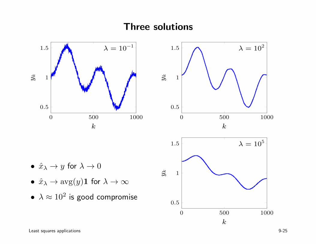
Three solutions
0 500 1000
0.5
1
1.5 λ = 10−1
k
yk
0 500 1000
0.5
1
1.5 λ = 102
k
yk
• xλ → y for λ→ 0
• xλ → avg(y)1 for λ→∞
• λ ≈ 102 is good compromise
0 500 1000
0.5
1
1.5 λ = 105
k
yk
Least squares applications 9-25

Image deblurring
y = Ax+ v
• x is unknown image, y is observed image
• A is (known) blurring matrix, v is (unknown) noise
• images are M ×N , stored as MN -vectors
blurred, noisy image y deblurred image x
Least squares applications 9-26

Least squares deblurring
minimize ‖Ax− y‖2 + λ(‖Dvx‖2 + ‖Dhx‖2)
• 1st term is ‘data fidelity ’ term: ensures Ax ≈ y
• 2nd term penalizes differences between values at neighboring pixels
‖Dhx‖2 + ‖Dvx‖2
=
M∑i=1
N−1∑j=1
(Xij −Xi,j+1)2 +
M−1∑i=1
N∑j=1
(Xij −Xi+1,j)2
if X is the M ×N image stored in the MN -vector x
Least squares applications 9-27

Differencing operations in matrix notation
suppose x is the M ×N image X, stored column-wise as MN -vector
x = (X1:M,1, X1:M,2, . . . , X1:M,N)
• horizontal differencing: (N − 1)×N block matrix with M ×M blocks
Dh =
I −I 0 · · · 0 0 00 I −I · · · 0 0 0...
......
......
...0 0 0 · · · 0 I −I
• vertical differencing: M ×M block matrix with (N − 1)×N blocks
Dv =
D 0 · · · 00 D · · · 0...
.... . .
...0 0 · · · D
, D =
1 −1 0 · · · 0 00 1 −1 · · · 0 0...
......
......
0 0 0 · · · 1 −1
Least squares applications 9-28

Deblurred images
results for λ = 10−6, λ = 10−4, λ = 10−2, λ = 1
Least squares applications 9-29

Outline
• model fitting
• multiobjective least squares
• control
• estimation
• statistics

Linear regression model
y = Xβ + ε
• ε is a random n-vector (random error or disturbance)
• β is (non-random) p-vector of unknown parameters
• X is an n× p matrix (‘design’ matrix, i.e., result of experiment design)
• y is an observable random n-vector
• this notation differs from previous sections but is common in statistics
• we discuss methods for estimating parameters β from observations of y
Least squares applications 9-30

Assumptions
• X is tall (n > p) with linearly independent columns
• random disturbances εi have zero mean
E εi = 0 for i = 1, . . . , n
• random disturbances have equal variances σ2
E ε2i = σ2 for i = 1, . . . , n
• random disturbances are uncorrelated (have zero covariances)
E(εiεj) = 0 for i, j = 1, . . . , n and i 6= j
last three assumptions can be combined using matrix and vector notation:
E ε = 0, E εεT = σ2I
Least squares applications 9-31

Least squares estimator
least squares estimate β of parameters β, given the observations y, is
β = X†y = (XTX)−1XTy
range(X) Xβ
ε
Xβ
e = y −Xβ
y = Xβ + ε
• Xβ is the orthogonal projection of y on range(X)
• residual e = y −Xβ is an (observable) random variable
Least squares applications 9-32

Mean and covariance of least squares estimate
β = X†(Xβ + ε) = β +X†ε
• least squares estimator is unbiased : E β = β
• covariance matrix of least squares estimate is
E (β − β)(β − β)T = E((X†ε)(X†ε)T
)= E
((XTX)−1XT εεTX(XTX)−1
)= σ2(XTX)−1
• covariance of βi and βj (i 6= j) is
E((βi − βi)(βj − βj)
)= σ2
((XTX)−1
)ij
for i = j, this is the variance of βi
Least squares applications 9-33

Estimate of σ2
Xβ
ε
Xβ
e = y −Xβ
y = Xβ + ε
E ‖ε‖2 = nσ2
E ‖e‖2 = (n− p)σ2
E ‖X(β − β)‖2 = pσ2
(proof on next page)
• define estimate σ of σ as
σ =‖e‖√n− p
• σ2 is an unbiased estimate of σ2:
E σ2 =1
n− pE ‖e‖2 = σ2
Least squares applications 9-34

Proof.
first expression is immediate: E ‖ε‖2 =∑ni=1E ε
2i = nσ2
• to show that E ‖X(β − β)‖2 = pσ2, first note that
X(β − β) = XX†y −Xβ= XX†(Xβ + ε)−Xβ= XX†ε
= X(XTX)−1XT ε
on line 3 we used X†X = I (however, note that XX† 6= I if X is tall!)
• squared norm of X(β − β) is
‖X(β − β)‖2 = εT (XX†)2ε = εTXX†ε
first step uses symmetry of XX†; second step, X†X = I
Least squares applications 9-35

• expected value of squared norm is
E ‖X(β − β)‖2 = E(εTXX†ε
)=
∑i,j
E(εiεj)(XX†)ij
= σ2n∑i=1
(XX†)ii
= σ2n∑i=1
p∑j=1
Xij(X†)ji
= σ2
p∑j=1
(X†X)jj
= pσ2
• expression E ‖e‖2 = (n− p)σ2 on page 9-34 now follows from
‖ε‖2 = ‖e+Xβ −Xβ‖2 = ‖e‖2 + ‖X(β − β)‖2
Least squares applications 9-36

Linear estimator
linear regression model (p.9-30), with same assumptions as before (p.9-31):
y = Xβ + ε
a linear estimator of β maps observations y to the estimate
β = By
• estimator is defined by the p× n matrix B
• least squares estimator is an example with B = X†
Least squares applications 9-37

Unbiased linear estimator
if B is a left inverse of X, then estimator β = By can be written as:
β = By = B(Xβ + ε) = β +Bε
• this shows that the linear estimator is unbiased (E β = β) if BX = I
• covariance matrix of unbiased linear estimator is
E((β − β)(β − β)T
)= E
(BεεTBT
)= σ2BBT
• if c is an (non-random) p-vector, then estimate cT β of cTβ has variance
E (cT β − cTβ)2 = σ2cTBBT c
least squares estimator is an example with B = X† and BBT = (XTX)−1
Least squares applications 9-38

Best linear unbiased estimator
if B is a left inverse of X then for all p-vectors c
cTBBT c ≥ cT (XTX)−1c
(proof on next page)
• left-hand side gives variance of cT β for linear unbiased estimator
β = By
• right-hand side gives variance of cT βls for least squares estimator
βls = X†y
• least squares estimator is the ‘best linear unbiased estimator ’ (BLUE)
this is known as the Gauss-Markov theorem
Least squares applications 9-39

Proof.
• use BX = I to write BBT as
BBT = (B − (XTX)−1XT )(BT −X(XTX)−1) + (XTX)−1
= (B −X†)(B −X†)T + (XTX)−1
• hence,
cTBBTC = cT (B −X†)(B −X†)T c+ cT (XTX)−1c
= ‖(B −X†)T c‖2 + cT (XTX)−1c
≥ cT (XTX)−1c
with equality if B = X†
Least squares applications 9-40