INSTITUTE OF PHYSICS PUBLISHING JOURNAL OF PHYSICS: CONDENSED MATTER

J. Phys.: Condens. Matter 14 (2002) 13551–13567 PII: S0953-8984(02)39697-8

Structural and magnetic properties of core–shelliron–iron oxide nanoparticles

L Theil Kuhn1,4, A Bojesen1, L Timmermann1, M Meedom Nielsen2 andS Mørup3

1 Ørsted Laboratory, Niels Bohr Institute for Astronomy, Physics and Geophysics,Universitetsparken 5, DK-2100 Copenhagen Ø, Denmark2 Danish Polymer Center, Risø National Laboratory, Frederiksborgvej 399, DK-4000 Roskilde,Denmark3 Department of Physics, Bldg 307, Technical University of Denmark, DK-2800 Kgs Lyngby,Denmark

E-mail: luise.theil.kuhn@risoe.dk

Received 17 July 2002Published 29 November 2002Online at stacks.iop.org/JPhysCM/14/13551

AbstractWe present studies of the structural and magnetic properties of core–shell iron–iron oxide nanoparticles. α-Fe nanoparticles were fabricated by sputtering andsubsequently covered with a protective nanocrystalline oxide shell consistingof either maghaemite (γ -Fe2O3) or partially oxidized magnetite (Fe3O4). Weobserved that the nanoparticles were stable against further oxidation, andMossbauer spectroscopy at high applied magnetic fields and low temperaturesrevealed a stable form of partly oxidized magnetite. The nanocrystallinestructure of the oxide shell results in strong canting of the spin structure inthe oxide shell, which thereby modifies the magnetic properties of the core–shell nanoparticles.

1. Introduction

Magnetic core–shell nanoparticles constitute systems with strong interactions betweendifferent magnetic and crystalline phases, which can result in exchange anisotropy andenhanced coercivity [1, 2]. From a technological point of view, the understanding ofthese magnetic properties is important. Often magnetic nanoparticles are covered with aprotective shell when they are used in technological applications. For example, iron–iron oxidenanoparticles are used in magnetic recording tapes [2, 3]. Studies of oxidation of nanoparticlescan also lead to improved understanding of corrosion processes.

As a consequence of their technological importance, iron–iron oxide nanoparticles havebeen investigated for decades. Several types of nanoparticle fabrication and structural and4 Present address: Materials Research Department, AFM-227, Risø National Laboratory, Frederiksborgvej 399,DK-4000 Roskilde, Denmark.

0953-8984/02/4913551+17$30.00 © 2002 IOP Publishing Ltd Printed in the UK 13551

13552 L T Kuhn et al

magnetic investigation techniques have been applied, see for instance [4–17]. There seems tobe a general agreement that the iron core has the bulk structural and magnetic properties of α-Fefor a wide range of nanoparticle sizes and shapes,e.g. 2–30 nm spherical nanoparticles [4, 9, 11]and acicular nanoparticles 100–360 nm long with aspect ratios up to 20 [5, 6]. Furthermore, theiron oxide surface layer consists of nanocrystallites 2–5 nm in size [4–6], or for special oxideformation conditions an epitaxial layer of similar thickness [17]. Often a spinel type iron oxidehas been observed, e.g. either maghaemite (γ -Fe2O3), magnetite (Fe3O4), non-stoichiometricpartially oxidized magnetite or mixtures of them. The presence of wustite (FeO) has also beenreported [10].

The lattice constants of the spinel structures magnetite (Fe3O4) and maghaemite (γ -Fe2O3) are quite similar. Therefore, they are not easily distinguished by x-ray diffraction.Mossbauer spectroscopy is a well suited technique for distinguishing these two oxide phases.In maghaemite, the spectral components due to the Fe3+ ions in A- and B-sites have similarMossbauer parameters and the spectrum can be described as a sextet, which is slightlyasymmetric. Line 6 is slightly broader and less intense than line 1, because of the smalldifferences between the isomer shifts and the magnetic hyperfine fields in the two sites. Inmagnetite, the B-sites contain equal amounts of Fe3+ and Fe2+ ions, but fast electron hoppingbetween these ions results in an effective valence state, Fe+2.5, for all B-site ions. The magnetichyperfine field of B-site ions in magnetite is therefore smaller than that of the A-site ions (Fe3+)and the isomer shift is larger. Thus, the A- and B-site contributions in the Mossbauer spectrumof magnetite can easily be distinguished. In bulk magnetite the electron hopping takes placeonly above the Verwey transition temperature, TV = 119 K. Below this temperature, theMossbauer spectrum consists of several sextets due to Fe2+ and Fe3+ ions. In nanoparticles ofmagnetite, the Verwey transition temperature is lower [18].

Mossbauer spectra with large applied magnetic fields give further information on thestructure and magnetic properties of the iron oxides. Perfect magnetite and maghaemite havea collinear ferrimagnetic order. When the magnetization is saturated by a large applied field, theA-site hyperfine field will be parallel and the B-site hyperfine field anti-parallel to the appliedfield. Therefore, the magnetic splitting of the A component is increased and the splitting ofthe B component is decreased. This allows the A and B components in maghaemite to bedistinguished if the applied field is sufficiently large. Furthermore, the relative intensities oflines 2 and 5 in the sextets will be affected by the applied field in a way that depends onthe angle between the field direction and the direction of the gamma rays. If the sample ismagnetized parallel to the gamma ray direction, lines 2 and 5 disappear in the spectrum. Insmall particles of magnetite and maghaemite, the spin structure is often non-collinear [19–23]. The canting may be localized at the nanoparticle surface, but defects in the interior ofmaghaemite nanoparticles may also induce canting [22, 23]. The spin canting can be studiedby Mossbauer spectroscopy with large magnetic fields. The relative intensity of the six linesis given by 3:x :1:1:x :3 with

x = 4 sin2 θ

1 + cos2 θ, (1)

where θ is the angle between the total magnetic field at the nucleus and the gamma raydirection [20]. Thus, the average canting angle can be estimated from the relative intensityof lines 2 and 5. Such studies are conveniently carried out with the applied field parallel tothe gamma ray direction. The magnetic splitting is proportional to the total magnetic field atthe nucleus, �Btot, which is given by the vector sum of the hyperfine field, �Bhf , and the appliedfield, �Bapp. Thus, Bhf can be found from the equation

B2hf = B2

tot + B2app − 2Btot Bapp cos θ. (2)

Structural and magnetic properties of core–shell iron–iron oxide nanoparticles 13553

We present here a combined structural and magnetic study of core–shell iron–iron oxidenanoparticles fabricated under different oxidation conditions. We have previously publishedresults on the magnetic properties of single iron–iron oxide nanoparticles measured by Hallmicro-magnetometry [25]. This study is focused on Mossbauer spectroscopy in the magneticfield range 0–6 T in the temperature range 5–295 K, and over a long time span (290 days). Wecontribute new results on the structural and the magnetic properties of the iron oxide surfacelayer.

The paper is organized as follows. In section 2 the experimental techniques are presented,in section 3 the crystal structure and the morphology of the nanoparticles is discussed and insections 4 and 5 the magnetic properties are discussed. In section 6, the domain structure of theα-Fe core is investigated. In section 7 the stability of the core–shell nanoparticles is discussed.Section 8 concludes the paper.

2. Experimental techniques

2.1. Nanoparticles

The nanoparticles were fabricated in a hollow cathode sputtering cluster source, describedin detail in [26]. A sputtering target (Fe) formed as a hollow cylinder was mounted in acondensation chamber and a sputtering gas (Ar, purity 99.998%) was led through at an appliedhigh voltage. The sputtering process produced a supersaturated metal vapour, and by severalstages of differential pumping of the Ar gas, the metal vapour was cooled and condensed intosolid metal clusters. The system is designed such that the clusters form a beam with lowkinetic energy and they can easily be deposited on any substrate without being damaged ordamaging the substrate, nor do the nanoparticles agglomerate after deposition. The substratewas kept at room temperature. The cluster source vacuum system had a background pressureof 10−5 Pa, and during nanoparticle production the Ar pressure was in the range 60–500 Pa inthe condensation chamber and in the differential pumping chambers it was reduced to 1, 10−2

and 10−4 Pa, respectively.For the experiments presented here two different types of sample were fabricated. Sample

A contained iron nanoparticles that were oxidized in a controlled way by exposing them to anincreasing pressure of oxygen following the scheme in table 1 and subsequently exposed to air.Sample B was exposed to air immediately after fabrication. To produce Mossbauer absorberswith a homogeneous distribution of nanoparticles, the nanoparticles were mixed with a BNpowder.

Table 1. Oxidation scheme for sample A. The total pressure of the oxygen–argon mixture was keptat 105 Pa.

O in Ar (mol%) Time (h)

0.02 11.00.20 6.52.00 1.0

2.2. Structural characterization

The nanoparticles were structurally characterized by transmission electron microscopy (TEM)and x-ray powder diffraction. The TEM samples were prepared by deposition of thenanoparticles on thin substrates of amorphous carbon film. The TEM studies were done

13554 L T Kuhn et al

with three instruments: a Philips CM20 (200 keV), a Philips EM430 (300 keV) and a Jeol3000 F (300 keV). X-ray powder diffraction was done on specially prepared nanoparticlesamples and on the as-prepared Mossbauer samples in a reflection geometry using a RigakuRotaflex 18 kW rotating anode with a Cu target. Pyrolithic graphite monochromators were usedbefore and after the sample to select the Cu Kα radiation (λ = 1.54(1) Å) and to suppress theFe Kα fluorescence. The beam geometry was defined by slits. The instrument calibration andbroadening was measured using a standard Si powder and the BN in the Mossbauer samples.

2.3. Mossbauer spectroscopy

Mossbauer spectra were obtained with a conventional constant-acceleration Mossbauerspectrometer using a 100 mCi source of 57Co in Rh. Spectra below 20 K and all spectrawith large applied fields (up to 6 T) were obtained using a liquid helium cryostat with asuperconducting magnet. The magnetic field was applied parallel to the gamma ray direction.Zero-field spectra at T � 20 K were obtained in a closed-cycle helium refrigerator. Isomershifts are given relative to that of α-Fe at room temperature. Room-temperature spectra withapplied fields of 0.55 T perpendicular to the gamma ray direction were obtained by use of anelectromagnet with an iron core.

3. Crystal structure and morphology of the nanoparticles

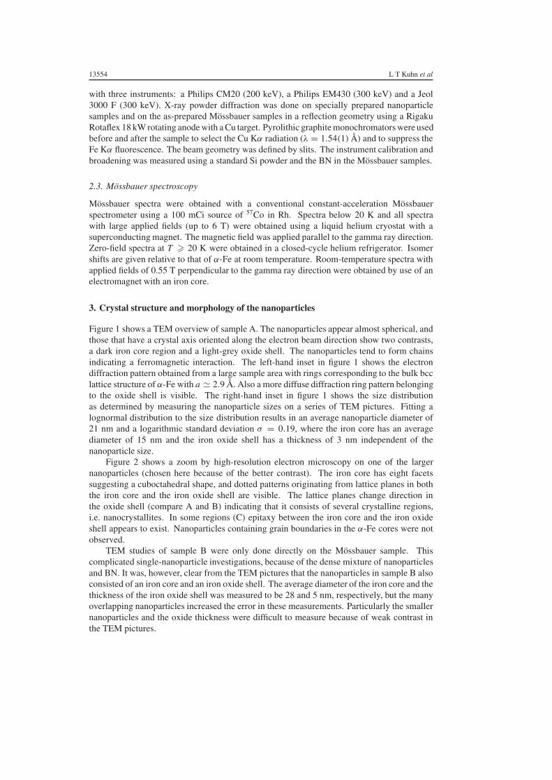
Figure 1 shows a TEM overview of sample A. The nanoparticles appear almost spherical, andthose that have a crystal axis oriented along the electron beam direction show two contrasts,a dark iron core region and a light-grey oxide shell. The nanoparticles tend to form chainsindicating a ferromagnetic interaction. The left-hand inset in figure 1 shows the electrondiffraction pattern obtained from a large sample area with rings corresponding to the bulk bcclattice structure of α-Fe with a � 2.9 Å. Also a more diffuse diffraction ring pattern belongingto the oxide shell is visible. The right-hand inset in figure 1 shows the size distributionas determined by measuring the nanoparticle sizes on a series of TEM pictures. Fitting alognormal distribution to the size distribution results in an average nanoparticle diameter of21 nm and a logarithmic standard deviation σ = 0.19, where the iron core has an averagediameter of 15 nm and the iron oxide shell has a thickness of 3 nm independent of thenanoparticle size.

Figure 2 shows a zoom by high-resolution electron microscopy on one of the largernanoparticles (chosen here because of the better contrast). The iron core has eight facetssuggesting a cuboctahedral shape, and dotted patterns originating from lattice planes in boththe iron core and the iron oxide shell are visible. The lattice planes change direction inthe oxide shell (compare A and B) indicating that it consists of several crystalline regions,i.e. nanocrystallites. In some regions (C) epitaxy between the iron core and the iron oxideshell appears to exist. Nanoparticles containing grain boundaries in the α-Fe cores were notobserved.

TEM studies of sample B were only done directly on the Mossbauer sample. Thiscomplicated single-nanoparticle investigations, because of the dense mixture of nanoparticlesand BN. It was, however, clear from the TEM pictures that the nanoparticles in sample B alsoconsisted of an iron core and an iron oxide shell. The average diameter of the iron core and thethickness of the iron oxide shell was measured to be 28 and 5 nm, respectively, but the manyoverlapping nanoparticles increased the error in these measurements. Particularly the smallernanoparticles and the oxide thickness were difficult to measure because of weak contrast inthe TEM pictures.

Structural and magnetic properties of core–shell iron–iron oxide nanoparticles 13555

Figure 1. TEM picture of sample A; the left-hand inset shows the obtained electron diffractionpattern, and the right-hand inset shows the size distribution for sample A as determined from theTEM pictures.

Figure 2. High-resolution electron microscopy picture of a single core–shell nanoparticle in sampleA. The dark core is the α-Fe and the light shell is the γ -Fe2O3/Fe3O4. Lattice planes in both regionsare visible. A smaller neighbouring nanoparticle is slightly overlapping at the top of the image.A–C refer to the text.

13556 L T Kuhn et al

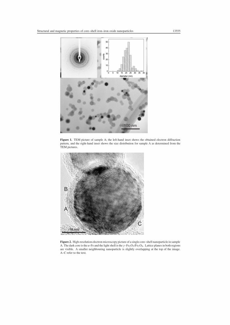
Figure 3. X-ray powder diffraction spectra from samples A and B. The background has beensubtracted and the peaks are marked with their respective origins: BN, α-Fe and Fe3O4/γ -Fe2O3with *. The spectra for A and B have been offset by 40 000 and 20 000, respectively. Also simulatedspectra for bulk Fe3O4 and γ -Fe2O3 are plotted.

Figure 3 shows the x-ray powder diffraction spectra for samples A and B performeddirectly on the Mossbauer prepared samples; these also include BN. The background in thespectra has been measured and subtracted and the peaks are marked according to their origins:BN, α-Fe and Fe3O4/γ -Fe2O3 with *. Simulated spectra for the bulk spinel structures Fe3O4

(a = 8.391 Å) and γ -Fe2O3 (a = 8.339 Å) [27] are also shown. The small sizes of thenanoparticles introduce a significant size and strain broadening of the diffraction features,thereby making the two spinel iron oxides indistinguishable. The diffraction spectra show notraces of other iron oxides such as wustite (FeO) or haematite (α-Fe2O3) nor other crystallinephases. The presence of the BN obstructed a valuable refinement of the spectra, therefore amore simplistic approach was chosen to evaluate the spectra: the background was subtractedand all the diffraction peaks were fitted with a sum of Gaussians and Lorentzians. The peaksoriginating from the nanoparticles were well fitted purely by Gaussians. The instrument

broadening was subtracted from the nanoparticle peaks following �cor =√

�2obs − �2

instr ,where �cor is the corrected FWHM, �obs is the observed FWHM and �instr is the FWHMof the instrumental broadening. The average size of the crystalline regions was obtained usingthe Scherrer formula [28]

d = Kλ

�(2θ) cos(θ), (3)

where K = 0.94, λ = 1.54 Å and �(2θ) is the FWHM of the diffraction peaks at angle 2θ .The analysis showed that the Fe components in samples A and B are very similar andthey originate from a bcc lattice with lattice constant a = 2.87 Å corresponding to bulkα-Fe [27]. For both samples, but particularly in sample B, an increasing broadening ofthe peaks with increasing 2θ beyond the instrumental broadening indicated the presence of

Structural and magnetic properties of core–shell iron–iron oxide nanoparticles 13557

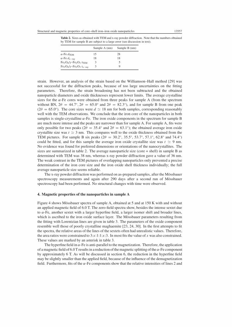
Table 2. Sizes as obtained with TEM and x-ray powder diffraction. Note that the numbers obtainedby TEM for sample B are subject to a large error (see discussion in text).

Sample A (nm) Sample B (nm)

α-Fe dTEM 15 28α-Fe dx−ray 18 18Fe3O4/γ -Fe2O3 tTEM 3 5Fe3O4/γ -Fe2O3 tx−ray 3 9

strain. However, an analysis of the strain based on the Williamson–Hall method [29] wasnot successful for the diffraction peaks, because of too large uncertainties on the fittingparameters. Therefore, the strain broadening has not been subtracted and the obtainednanoparticle diameters and oxide thicknesses represent lower limits. The average crystallinesizes for the α-Fe cores were obtained from three peaks for sample A (from the spectrumwithout BN, 2θ = 44.7◦, 2θ = 65.0◦ and 2θ = 82.3◦), and for sample B from one peak(2θ = 65.0◦). The core sizes were d � 18 nm for both samples, corresponding reasonablywell with the TEM observations. We conclude that the iron core of the nanoparticles in bothsamples is single-crystalline α-Fe. The iron oxide components in the spectrum for sample Bare much more intense and the peaks are narrower than for sample A. For sample A, fits wereonly possible for two peaks (2θ = 35.4◦ and 2θ = 63.1◦); the obtained average iron oxidecrystallite size was t � 3 nm. This compares well to the oxide thickness obtained from theTEM pictures. For sample B six peaks (2θ = 30.2◦, 35.5◦, 53.7◦, 57.1◦, 62.8◦ and 74.4◦)could be fitted, and for this sample the average iron oxide crystallite size was t � 9 nm.No evidence was found for preferred dimensions or orientations of the nanocrystallites. Thesizes are summarized in table 2. The average nanoparticle size (core + shell) in sample B asdetermined with TEM was 38 nm, whereas x-ray powder diffraction gave a value of 36 nm.The weak contrast in the TEM pictures of overlapping nanoparticles only prevented a precisedetermination of the iron core size and the iron oxide shell thickness individually; the fullaverage nanoparticle size seems reliable.

The x-ray powder diffraction was performed on as-prepared samples, after the Mossbauerspectroscopy measurements and again after 290 days after a second run of Mossbauerspectroscopy had been performed. No structural changes with time were observed.

4. Magnetic properties of the nanoparticles in sample A

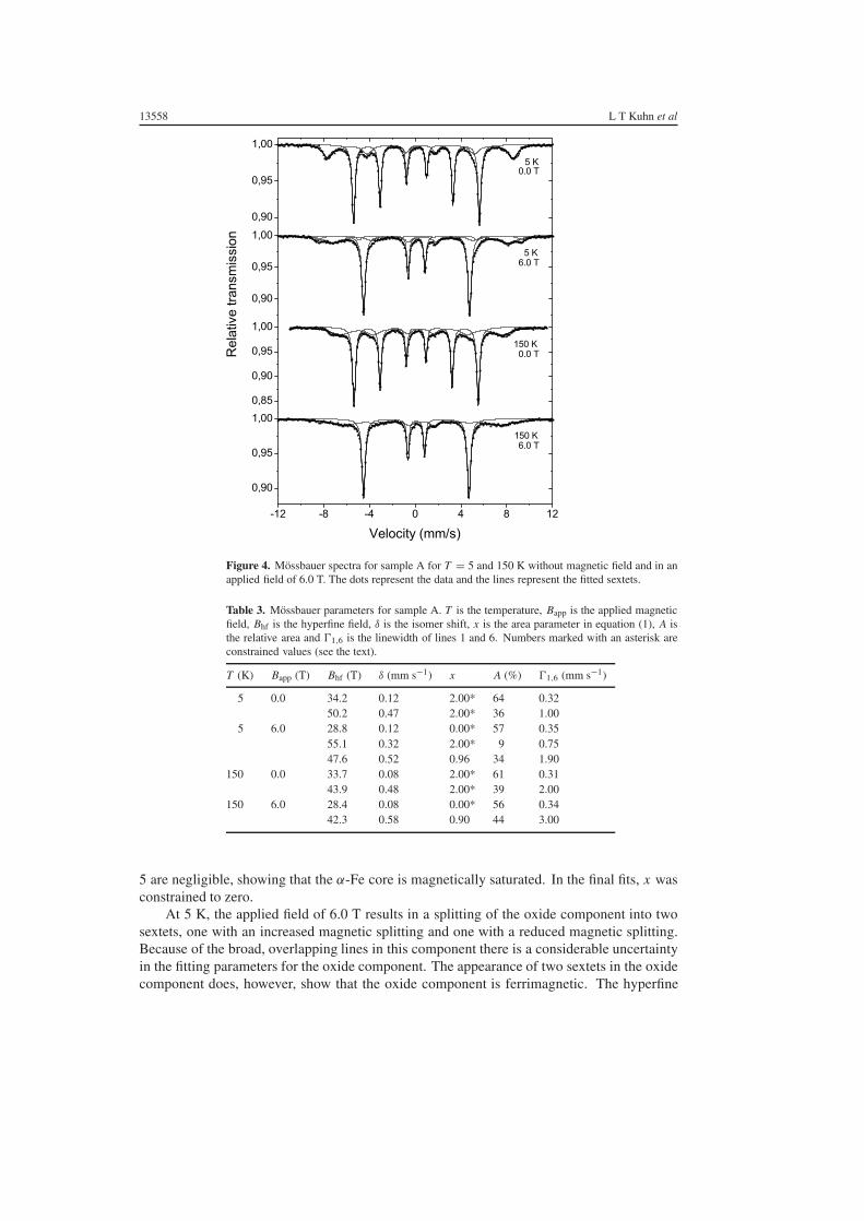
Figure 4 shows Mossbauer spectra of sample A, obtained at 5 and at 150 K with and withoutan applied magnetic field of 6.0 T. The zero-field spectra show, besides the intense sextet dueto α-Fe, another sextet with a larger hyperfine field, a larger isomer shift and broader lines,which is ascribed to the iron oxide surface layer. The Mossbauer parameters resulting fromthe fitting with Lorentzian lines are given in table 3. The parameters of the oxide componentresemble well those of poorly crystalline maghaemite [23, 24, 30]. In the first attempts to fitthe spectra, the relative areas of the lines of the sextets often had unrealistic values. Therefore,the area ratios were constrained to 3:x :1:1:x :3. In most fits the value of x was also constrained.These values are marked by an asterisk in table 3.

The hyperfine field in α-Fe is anti-parallel to the magnetization. Therefore, the applicationof a magnetic field of 6.0 T results in a reduction of the magnetic splitting of the α-Fe componentby approximately 6 T. As will be discussed in section 6, the reduction in the hyperfine fieldmay be slightly smaller than the applied field, because of the influence of the demagnetizationfield. Furthermore, fits of the α-Fe components show that the relative intensities of lines 2 and

13558 L T Kuhn et al

Figure 4. Mossbauer spectra for sample A for T = 5 and 150 K without magnetic field and in anapplied field of 6.0 T. The dots represent the data and the lines represent the fitted sextets.

Table 3. Mossbauer parameters for sample A. T is the temperature, Bapp is the applied magneticfield, Bhf is the hyperfine field, δ is the isomer shift, x is the area parameter in equation (1), A isthe relative area and �1,6 is the linewidth of lines 1 and 6. Numbers marked with an asterisk areconstrained values (see the text).

T (K) Bapp (T) Bhf (T) δ (mm s−1) x A (%) �1,6 (mm s−1)

5 0.0 34.2 0.12 2.00* 64 0.3250.2 0.47 2.00* 36 1.00

5 6.0 28.8 0.12 0.00* 57 0.3555.1 0.32 2.00* 9 0.7547.6 0.52 0.96 34 1.90

150 0.0 33.7 0.08 2.00* 61 0.3143.9 0.48 2.00* 39 2.00

150 6.0 28.4 0.08 0.00* 56 0.3442.3 0.58 0.90 44 3.00

5 are negligible, showing that the α-Fe core is magnetically saturated. In the final fits, x wasconstrained to zero.

At 5 K, the applied field of 6.0 T results in a splitting of the oxide component into twosextets, one with an increased magnetic splitting and one with a reduced magnetic splitting.Because of the broad, overlapping lines in this component there is a considerable uncertaintyin the fitting parameters for the oxide component. The appearance of two sextets in the oxidecomponent does, however, show that the oxide component is ferrimagnetic. The hyperfine

Structural and magnetic properties of core–shell iron–iron oxide nanoparticles 13559

fields are changed by less than the value of the applied field, and the non-zero relative intensityof lines 2 and 5 shows that there is a strong canting of the spins in the oxide. The relativearea of the high-field component is apparently less than one-third of the relative area of thelow-field oxide component in the 6.0 T spectrum. This is less than the expected values forperfect maghaemite (≈0.6) or magnetite (≈0.5). However, similar results were earlier foundin studies of poorly crystalline maghaemite nanoparticles [23].

At 150 K, the lines of the oxide component in both the zero-field spectrum and the 6.0 Tspectrum are considerably broadened, and it is not possible to distinguish two oxide sextets inthe 6.0 T spectrum. The oxide component in this spectrum was therefore fitted with one sextet.The average hyperfine fields at 150 K are considerably smaller than those found at 5 K andalso much smaller than the bulk value [31]. These observations can be explained by transverserelaxation, i.e. fluctuations of components of the magnetization, which are perpendicular to thedirection of the average magnetization [30]. There is no indication of the presence of a sextetwith hyperfine field and isomer shift corresponding to the Fe2.5+ component in magnetite inthe spectra obtained at 150 K. Thus the results indicate that the iron oxide shell covering theα-Fe nanoparticles in sample A consists of maghaemite with a disordered spin canted magneticstructure.

5. Magnetic properties of the nanoparticles in sample B

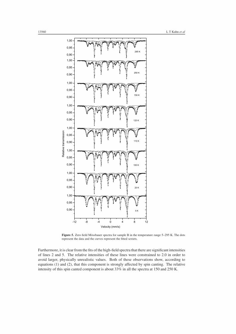
Mossbauer spectra of sample B, obtained without and with applied magnetic fields up to 6.0 Tin the temperature range 5–295 K, are shown in figures 5 and 6, respectively. The fittingparameters of the Lorentzian lines for the corresponding spectra are given in table 4. Therelative areas of the lines in the sextets were constrained as discussed in section 4.

As in the spectra for sample A an α-Fe sextet is present, but the spectra for sample B showa more pronounced pattern originating from the oxide. In the zero-field spectrum at 5 K, theoxide component can as a first approximation be described by one sextet. When a magneticfield of 6.0 T is applied, it splits up into two sextets in a way that is qualitatively similar tothat seen for sample A. Both components exhibit spin canting, as evidenced from the non-zerovalues of the parameter x in table 4. At higher temperatures, the spectra of sample B are notablydifferent from those of sample A. The zero-field spectra, obtained at T � 100 K, contain twooxide sextets with different isomer shifts and magnetic hyperfine fields. In fact, the Mossbauerparameters of the two sextets are similar to those of magnetite with the high-field componentdue to Fe3+ at the A-sites and the low-field component due to Fe2.5+ at B-sites of the spinellattice [24, 31]. In pure stoichiometric magnetite, the number of B-site iron atoms is twicethe number of A-site iron atoms. The ratio of the spectral areas of the B and A componentsis therefore close to two. Although the uncertainty of the relative areas in the present case islarge because of broad overlapping lines, the fits of the zero-field spectra indicate that the ratiois considerably smaller than 2. This shows that the iron oxide cannot be described as purestoichiometric magnetite.

When large magnetic fields are applied at T � 100 K, the oxide component can bedescribed as consisting of three sextets, in contrast to the spectrum of pure magnetite, whichremains a superposition of two sextets. The analysis of the relative areas and the hyperfineparameters of these three components give new information on the composition of the oxidelayer. For example, the spectra obtained at 150 K show for Bapp = 0 T a component with ahyperfine field Bhf = 46.7 T and an isomer shift δ = 0.65 mm s−1, which are parameters verysimilar to those of the B-site Fe2.5+ component of magnetite, but the lines are considerablybroadened. When a magnetic field is applied, the magnetic splitting of this component isreduced, but the reduction is less than that corresponding to the value of the applied field.

13560 L T Kuhn et al

Figure 5. Zero field Mossbauer spectra for sample B in the temperature range 5–295 K. The dotsrepresent the data and the curves represent the fitted sextets.

Furthermore, it is clear from the fits of the high-field spectra that there are significant intensitiesof lines 2 and 5. The relative intensities of these lines were constrained to 2.0 in order toavoid larger, physically unrealistic values. Both of these observations show, according toequations (1) and (2), that this component is strongly affected by spin canting. The relativeintensity of this spin canted component is about 33% in all the spectra at 150 and 250 K.

Structural and magnetic properties of core–shell iron–iron oxide nanoparticles 13561

Figure 6. Mossbauer spectra for sample B showing the effect of applying a magnetic field up to6.0 T at various temperatures between 5 and 250 K. The dots represent the data and the curvesrepresent the fitted sextets.

The second iron oxide component, seen in the zero-field spectrum at 150 K, has a magnetichyperfine field Bhf = 50.6 T and an isomer shift δ = 0.37 mm s−1. These values are closeto those for Fe3+ in A-sites in magnetite and for Fe3+ ions in both A-sites and B-sites inmaghaemite. When magnetic fields are applied, the component splits up into two sextets. AtBapp = 6.0 T, the magnetic splittings of the two components are increased or decreased byamounts corresponding to approximately the value of the applied field. The spectra are wellfitted with zero intensity of lines 2 and 5 in these two components. These results show that theFe3+ ions are distributed between A- and B-sites. The relative areas of the two Fe3+ sextets aresimilar, indicating that the numbers of Fe3+ ions on A-sites and B-sites are similar. The spectraobtained at 100 K show the same trends, but as the linewidths are larger at this temperature, the

13562 L T Kuhn et al

Table 4. Mossbauer parameters for sample B. T is the temperature, Bapp is the applied magneticfield, Bhf is the hyperfine field, δ is the isomer shift, x is the area parameter in equation (1), A isthe relative area and �1,6 is the linewidth of lines 1 and 6. Numbers marked with an asterisk areconstrained values (see the text).

T (K) Bapp (T) Bhf (T) δ (mm s−1) x A (%) �1,6 (mm s−1)

5 0.0 34.1 0.12 2.00* 40 0.3151.0 0.44 2.00* 49 0.8053.0 0.72 2.00* 11 0.37

5 6.0 28.8 0.12 0.00* 36 0.3647.5 0.53 0.74 42 0.9256.2 0.36 1.36 22 0.58

100 0.0 33.9 0.10 2.00* 40 0.3046.6 0.67 2.00* 24 1.4250.9 0.41 2.00* 36 0.67

100 6.0 28.6 0.11 0.00* 33 0.3544.0 0.84 1.24 23 1.5347.1 0.46 0.54 27 0.8556.1 0.38 0.72 17 0.59

150 0.0 33.7 0.08 2.00* 41 0.3046.7 0.65 2.00* 32 1.4550.6 0.37 2.00* 27 0.59

150 2.0 32.1 0.09 0.00* 35 0.3646.3 0.67 2.00* 38 1.2450.3 0.35 0.00* 18 0.6152.1 0.42 1.02 9 0.36

150 4.0 30.3 0.09 0.00* 38 0.3645.8 0.83 2.00* 30 1.1248.1 0.35 0.00* 10 0.4854.1 0.35 0.00* 10 0.48

150 6.0 28.5 0.09 0.00* 37 0.3543.1 0.77 2.00* 32 1.2646.6 0.41 0.00* 17 0.7456.0 0.35 0.00* 14 0.60

250 0.0 33.3 0.02 2.00* 45 0.3145.6 0.61 2.00* 33 1.4349.5 0.30 2.00* 22 0.48

250 4.0 30.0 0.04 0.00* 38 0.3443.3 0.70 2.00* 36 1.1847.2 0.33 0.00* 14 0.7253.6 0.31 0.00* 12 0.52

uncertainties are larger. The results obtained at 250 K are also consistent with those obtainedat 150 K.

The data obtained above 100 K may be explained by the presence of a mixture ofmaghaemite and magnetite or by a partially oxidized magnetite. It is difficult to distinguishbetween these from high-field Mossbauer spectra above the Verwey temperature [32].However, the spectra obtained at lower temperatures can further elucidate the nature of theoxide shell.

It is surprising that although there is a substantial number of Fe2.5+ ions visible in thespectra obtained at T � 100 K, there are no visible Fe2+ lines in the spectra obtained at 5 K.In perfect bulk magnetite, the Verwey transition is a first-order transition, which takes placeat T = 119 K. In nanoparticles, the transition takes place at a lower temperature than in

Structural and magnetic properties of core–shell iron–iron oxide nanoparticles 13563

bulk. Earlier studies of magnetite nanoparticles as small as 6 nm have shown the presence of aVerwey transition such that the 5 K spectrum of the nanoparticles was almost identical to thatof bulk magnetite with several visible lines due to Fe2+ [18]. The magnetic hyperfine fieldsof the Fe2+ components, which were expected to be visible at 5 K, are very sensitive to localdistortions caused by, for example, defects, because of the orbital contribution to the magnetichyperfine field. Therefore, if there are variations of the local environments of the Fe2+ ions, theFe2+ components may be smeared out such that they are not visible as separate components.The results of the present study therefore indicate that the oxide component is not a mixtureof magnetite and maghaemite, but rather a partly oxidized magnetite.

6. Demagnetization fields in the α-Fe cores

Small ferromagnetic particles may be single-domain or multi-domain particles dependingon the particle size. In single-domain particles, the atoms in the interior are exposed tothe demagnetizing field, which is formed by the uncompensated poles at the surface. Thevalue depends on the nanoparticle shape, the magnetization and the magnetization direction.The demagnetizing field is anti-parallel to the magnetization direction. For spherical single-domain α-Fe nanoparticles, the demagnetizing field equals 0.7 T [33, 34]. For an infinitefilm magnetized in the film plane, the demagnetizing field vanishes. If a nanoparticle is largeenough to form domains, the poles at the surface may disappear, resulting in the disappearanceof the demagnetizing field. If a multi-domain particle is exposed to a sufficiently large magneticfield, the domain structure is broken down such that it becomes a single-domain particle witha non-zero demagnetization field [33].

In 57Fe Mossbauer spectroscopy one can measure the magnetic field at the nuclei with aprecision better than 0.05 T. Therefore, Mossbauer spectroscopy of ferromagnetic materialscan be used to study demagnetizing fields, i.e. it can give information on the domain structureof small particles [33, 34]. If the ferromagnetic nanoparticles are not well separated, the nucleiwill also feel a magnetic field arising from the dipole field of the neighbouring nanoparticles.The total contribution to the field at a nucleus in a spherical nanoparticle is given by [33, 34]

�Btot = �Bhf + �Bdem + �Bdip + �Bapp. (4)

The first term represents the hyperfine field, the second term the demagnetizing field, the thirdterm the dipole field from the neighbouring nanoparticles and the fourth term the applied field.Calculating the dipole term is complicated since it depends on the geometrical arrangementand the orientation of the magnetization of the neighbouring nanoparticles.

To get information about the domain structure of the α-Fe cores in our samples, wehave obtained room-temperature Mossbauer spectra with and without a magnetic field of0.55 ± 0.01 T applied parallel to the sample plane. Similar measurements were made on athin calibration foil of α-Fe. The values of Btot for the α-Fe components are given in table 5.The uncertainty on Btot is 0.03 T. For the iron foil, the application of the magnetic field resultsin a reduction of Btot by 0.54 T, which is very close to the value of the applied field. This is asexpected because the demagnetizing field is close to zero for a thin foil. For samples A andB, Btot is reduced by only 0.17 and 0.16 T, respectively, when the magnetic field is applied.

Based on the structural characterization we can assume that the nanoparticles are closeto being spherical. The contributions of the applied field and the demagnetizing field shouldtherefore result in an increase of Btot by 0.15 T. These results suggest that the dipole field fromneighbouring nanoparticles is not negligible, and it is approximately 0.3 T. Earlier experimentalstudies as well as Monte Carlo simulations on samples of non-oxidized α-Fe nanoparticlesarranged in chains yielded values of about 0.4 T for the dipole interaction [34]. The lower value

13564 L T Kuhn et al

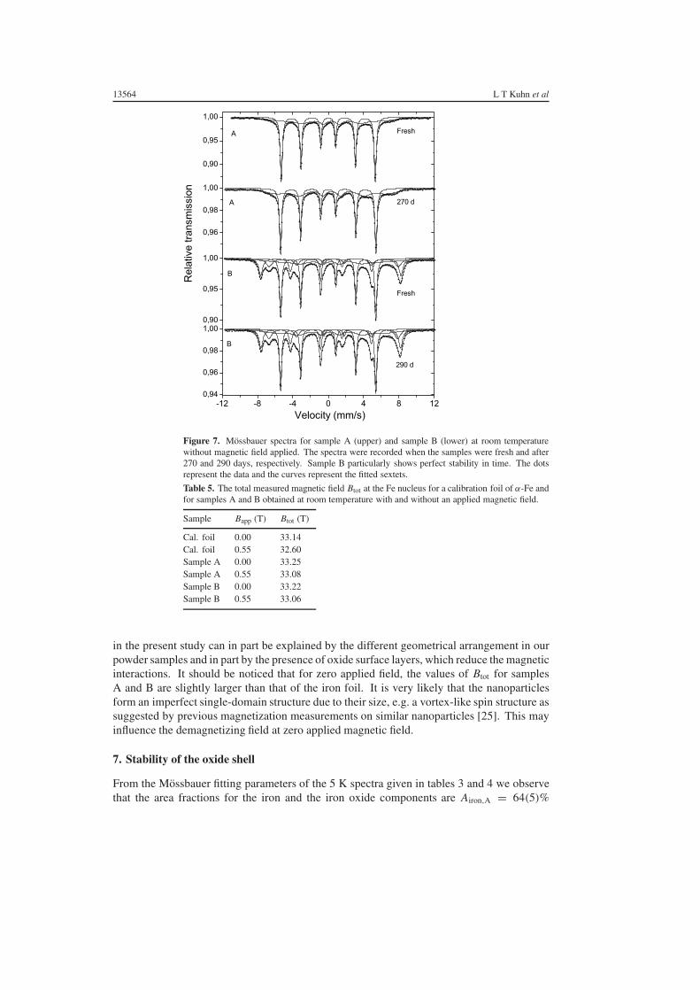
Figure 7. Mossbauer spectra for sample A (upper) and sample B (lower) at room temperaturewithout magnetic field applied. The spectra were recorded when the samples were fresh and after270 and 290 days, respectively. Sample B particularly shows perfect stability in time. The dotsrepresent the data and the curves represent the fitted sextets.

Table 5. The total measured magnetic field Btot at the Fe nucleus for a calibration foil of α-Fe andfor samples A and B obtained at room temperature with and without an applied magnetic field.

Sample Bapp (T) Btot (T)

Cal. foil 0.00 33.14Cal. foil 0.55 32.60Sample A 0.00 33.25Sample A 0.55 33.08Sample B 0.00 33.22Sample B 0.55 33.06

in the present study can in part be explained by the different geometrical arrangement in ourpowder samples and in part by the presence of oxide surface layers, which reduce the magneticinteractions. It should be noticed that for zero applied field, the values of Btot for samplesA and B are slightly larger than that of the iron foil. It is very likely that the nanoparticlesform an imperfect single-domain structure due to their size, e.g. a vortex-like spin structure assuggested by previous magnetization measurements on similar nanoparticles [25]. This mayinfluence the demagnetizing field at zero applied magnetic field.

7. Stability of the oxide shell

From the Mossbauer fitting parameters of the 5 K spectra given in tables 3 and 4 we observethat the area fractions for the iron and the iron oxide components are Airon,A = 64(5)%

Structural and magnetic properties of core–shell iron–iron oxide nanoparticles 13565

and Aoxide,A = 36(5)%, and Airon,B = 40(5)% and Aoxide,B = 60(5)% for samples A andB, respectively5. Thus, we can estimate the thickness of the iron oxide shell assuming thatthe sizes of iron cores obtained by x-ray powder diffraction are correct, and that the bulkdensities apply to our nanoparticles (ρiron = 7848 kg m−3, ρmaghaemite = 5490 kg m−3 andρmagnetite = 5210 kg m−3 [27]). Then, for sample A the thickness of the maghaemite shellbecomes tA � 3 nm, and for sample B the partly oxidized magnetite shell thickness becomestB � 6 nm. Taking the uncertainties into account, this agrees well with the results of thestructural characterization by TEM and x-ray powder diffraction.

It is important to note that within the experimental error, the total areas in the Mossbauerspectra do not show any substantial temperature dependence in the measured temperature range5–295 K, and the Debye–Waller factor is not much different from that of the bulk material.Furthermore, the area fractions for both samples A and B show no change in the temperaturerange 5–295 K. This means that the effective Debye–Waller factors, and thereby also theeffective Debye temperatures, for the iron core and the iron oxide shell are equal. This is inopposition to the results of some earlier studies [7, 8], where it was observed that the iron oxidenanocrystallites had a lower apparent Debye temperature than the α-Fe core, i.e. the iron oxidenanocrystallites were slightly detached from the iron core and could vibrate separately.

Immediately after the samples were prepared, they were transferred to vacuum, and themeasurements at both room temperature and lower temperature were carried out in vacuum inorder to limit further oxidation during the measurements. After most of the low-temperaturemeasurements had been carried out, the samples were kept in air and occasionally a Mossbauerspectrum was recorded at room temperature in order to follow the oxidation of the nanoparticles.Figure 7 shows room-temperature Mossbauer spectra of samples A and B as freshly preparedand after 270 and 290 days, respectively. In sample A, there seems to be a small increase inthe amount of oxide. The lines of the oxide component appear to become sharper and moreintense after the long exposure to air as also observed in [11]. However, the fits of the spectradid not give clear evidence for a change of the area ratio of the α-Fe component and the oxidecomponent. Sample B seems very little affected by the exposure to air. This means that therelative amount of oxidized iron is close to being constant. Furthermore, the degree of oxidationof the partially oxidized magnetite is also found to be unaffected by the exposure to air.

The evolution with time t of the oxidation of Fe can be described by the Carberra–Mottequation [11]

t = x2

Ax0e−x0/x , (5)

where x is the thickness of the formed oxide layer, x0 = 8 × 10−8 m is a material constantfor the oxide and A � 5.4 × 10−30 m s−1 is the growth velocity constant. These constantsare valid at T = 295 K. This means that the α-Fe nanoparticle oxide evolves from 1 nm att = 0.2 fs to 2 nm at t = 40 s and to 3 nm at t = 40 weeks. At higher temperature the oxidegrows faster.

Comparing the structural and magnetic properties of samples A and B, the observationof the thick, extremely stable, partly oxidized magnetite shell is striking. We suggest that thenanoparticles in sample A behave and evolve as expected according to the Carberra–Mott modelbecause the oxide shell was formed under controlled conditions, whereas the sudden exposureto air for sample B caused the nanoparticles to oxidize in a very abrupt way presumably underelevated temperature for a short while (other samples were observed to burst into sparks when

5 The error on the area fractions for the fitted iron sextets is approximately ±5%. On the individual oxide componentsthe error is in some cases larger because of the very broad lines.

13566 L T Kuhn et al

suddenly exposed to air). As the nanoparticles were cooled by the surrounding air, the violentoxidation stopped and an iron oxide in a frozen state resulted.

8. Conclusion

In conclusion, we have observed that facetted single-crystalline α-Fe nanoparticles exposedto different oxidation conditions formed different phases of nanocrystalline iron oxide shells.The core–shell nanoparticles proved to be structurally strained and very rigid, and we suggestthat this is caused by the perfect crystallinity and purity of the iron nanoparticles before theoxide was formed. The iron oxide shell formed under controlled oxidation conditions inan oxygen/argon atmosphere at room temperature was shown to be maghaemite (γ -Fe2O3).The maghaemite shell grew very slowly in time. The iron oxide shell formed when the ironnanoparticles were exposed to sudden violent oxidation in air consisted of a partly oxidizedphase of magnetite (non-stoichiometric Fe3O4), which proved to be extremely stable in time.This particular frozen form of partly oxidized magnetite was revealed through Mossbauerspectroscopy between 5 and 295 K in applied magnetic fields up to 6 T.

The Mossbauer spectra showed that the nanoparticles in both samples A and B behavedlike ferromagnetic cores with strongly frustrated spin canted magnetic shells, and nosuperparamagnetic effects were observed. This all points to the presence of strong magneticinteractions between the α-Fe core and the γ -Fe2O3 and the Fe3O4 shells. The analysis ofthe demagnetization measurements indicated that the iron core of the nanoparticles formed animperfect single-domain structure, and that the iron oxide surface layer reduced the magneticinteractions between the nanoparticles.

Acknowledgments

The authors would like to thank E Johnson and F Grumsen for transmission electron microscopystudies. The authors are indebted to H K Rasmussen for technical assistance. The financialsupport provided by the Danish Natural Science Research Council and the Danish TechnicalResearch Council is gratefully acknowledged.

References

[1] Cullity B D 1972 Introduction to Magnetic Materials (Reading, MA: Addison-Wesley)[2] O’Handley R 2000 Modern Magnetic Materials (New York: Wiley)[3] Morales M P, Walton S A, Prichard L S, Serna C J, Dickson D P E and O’Grady K 1998 J. Magn. Magn. Mater.

190 357[4] Haneda K and Morrish A H 1978 Surf. Sci. 77 584[5] Kishimoto M, Kitahata S and Amemiya M 1986 IEEE Trans. Magn. 200 732[6] Maeda Y, Aramaki M, Takashima Y, Oogai M and Goto T 1987 Bull. Chem. Soc. Japan 60 3241[7] Tamura I and Hayashi M 1992 Japan. J. Appl. Phys. 31 2540[8] Huang R, Xiong H, Lu Q, Hsia Y, Liu R, Ji R, Lu H, Wang L, Xu Y and Fang G 1993 J. Appl. Phys. 74 4102[9] Bødker F, Mørup S and Linderoth S 1994 Phys. Rev. Lett. 72 282

[10] Sethi S A, Pedersen M S, Tholen A R and Mørup S 1994 Nanophase Materials ed G C Hadjipanayis andR W Siegel (Dordrecht: Kluwer) p 81

[11] Linderoth S, Mørup S and Bentzon M D 1995 J. Mater. Sci. 30 3142[12] Parker F T, Spada F E, Cox T J and Berkowitz A E 1995 J. Appl. Phys. 77 5853[13] Jonsson B J, Turkki T, Strom V, El-Shall M S and Rao K V 1996 J. Appl. Phys. 79 5063[14] Zhao X Q, Liu B X, Liang Y and Hu Z Q 1996 J. Magn. Magn. Mater. 164 401[15] Kim H-J, Park J-H and Vescovo E 2000 Phys. Rev. B 61 15284[16] Banarjee S, Roy S, Chan J W and Chakravorty D 2000 J. Magn. Magn. Mater. 219 45

Structural and magnetic properties of core–shell iron–iron oxide nanoparticles 13567

[17] Kwok Y S, Zhang X X, Qin B and Fung K K 2000 Appl. Phys. Lett. 77 3971[18] Mørup S and Topsøe H 1983 J. Magn. Magn. Mater. 31–34 953[19] Coey J M D 1971 Phys. Rev. Lett. 27 1140[20] Morrish A H and Haneda K 1983 J. Magn. Magn. Mater. 35 105[21] Coey J M D 1987 Can. J. Phys. 65 1210[22] Morales M P, Serna F, Bødker F and Mørup S 1997 J. Phys.: Condens. Matter 9 5461[23] Serna C J, Bødker F, Mørup S, Morales M P, Santiumenge F and Veintemillas-Verdaguer S 2001 Solid State

Commun. 118 437[24] de Grave E, da Costa G M, Bowen L H, Barrero C A and Vandenberghe R E 1998 Hyperfine Interact. 117 245[25] Kuhn L T, Geim A K, Lok J G S, Hedegård P, Ylanen K, Jensen J B, Johnson E and Lindelof P E 2000 Eur.

Phys. J. D 10 259[26] Kuhn L T 1999 PhD Thesis University of Copenhagen[27] Mineral database on www.webmineral.com[28] Warren B E 1990 X-Ray Diffraction (New York: Dover)[29] Gerward L 2001 X-Ray Analytical Methods (Kgs. Lyngby: Technical University of Denmark)[30] Tronc E, Ezzir A, Cherkaoui R, Chaneac C, Nogues M, Kachkachi H, Fiorani D, Testa A M, Greneche J M and

Jolivet J P 2000 J. Magn. Magn. Mater. 221 63[31] Murad E 1998 Hyperfine Interact. 111 251[32] Vandenberghe R E, Barrero C A, da Costa G M, Van San E and de Grave E 2000 Hyperfine Interact. 126 247[33] Knudsen J E and Mørup S 1980 J. Physique 41 C1-155[34] von Eynatten G and Bommel H E 1977 Appl. Phys. 14 415