OPTIMAL INFORMATION THEORETIC CAPACITYOF THE PLANAR CELLULAR UPLINK CHANNEL

Symeon Chatzinotas, Muhammad Ali Imran, Costas Tzaras

Centre for Communication Systems Research, University of Surrey, United Kingdom, GU2 7XH

196

ABSTRACT

The majority of information-theoretic hyper-receiver cellu­lar models preserve a fundamental assumption which has ini­tially appeared in Wyner's [1] model, namely the collocationof User Terminals (UTs). Although this assumption producesmore tractable mathematical models, it is unrealistic with re­spect to current practical cellular systems. In this paper, wealleviate this assumption by assuming uniformly distributedUTs. The model under investigation is a Gaussian CellularMultiple Access Channel (GCMAC) over a planar cellular ar­ray in the presence of power-law path loss and flat fading. Inthis context, we evaluate the effect of UT distribution on theoptimal sum-rate capacity by considering a variable-densitycellular system. Furthermore, we compare the sum-rate ca­pacity produced by the planar and the linear cellular array.Finally, the analytical results are interpreted in the context ofa typical macrocellular scenario.

1. INTRODUCTION

The first concrete result for the information-theoretic capac­ity of the Gaussian Cellular Multiple Access Channel (GC­MAC) was presented by Wyner in [1]. Using a very sim­ple but tractable model for the cellular uplink channel, Wynershowed the importance of joint decoding at the Base Station(BS) receivers (hyper-receiver) and found the analytical for­mulas of the maximum system capacity. This model triggeredthe interest of the research community in the cellular capac­ity limits and was extended in [2] to include flat fading en­vironments. One major assumption shared in these modelswas that the cell density is fixed and only physically adjacentcells interfere. The author in [3], extended the model by as­suming multiple-tier interference and incorporated a distance­dependent path loss factor in order to study the effect of celldensity in a linear cellular array. However, the assumption

The work reported in this paper has formed part of the "FundamentalLimits to Wireless Network Capacity" Elective Research Programme of theVrrtual Centre of Excellence in Mobile & Personal Communications, MobileVCE, www.mobilevce.com.This research has been funded by the followingIndustrial Companies who are Members of Mobile VCE - BBC, BT, Huawei,Nokia, Nokia Siemens Networks, Nortel, Vodafone. Fully detailed technicalreports on this research are available to staff from these Industrial Membersof Mobile VCE. The authors would like to thank Prof. G. Caire and Prof. D.Tse for the useful discussions.

978-1-4244-2046-9/08/$25.00 ©2008 IEEE

of collocation of all UTs in each cell was maintained to keepthe model tractable. In this paper, we extend these models inorder to incorporate the effect of user distribution. Instead ofassuming collocated UTs, we assume that UTs are spatiallydistributed within the cell and each channel gain is affectedby a distance-dependent path loss factor. The rest of the pa­per is organised as follows. In the next section, we describethe proposed model and we describe the derivation of the in­formation theoretic capacity of the cellular system. In section3, we evaluate and compare the capacity results produced byboth simulation and analysis. In addition, section 4 interpretsthe analytical results in the context of a typical macrocellularscenario. The last section concludes the paper.

2. MODEL DESCRIPTION AND ANALYSIS

Assume that the K users are uniformly distributed in eachcell of a planar cellular system comprising N base stations.Assuming flat fading, the received signal at cell n, at timeindex t, will be given by:

N K

yn[t] = L L c;'kmg;:m[t]Xk[t] + zn[t] (1)m=l k=l

where xr [t] is the tth complex channel symbol transmittedby the kth UT of the mth cell and {gkm } are independent,strictly stationary and ergodic complex random processes inthe time index t, which represent the flat fading processes ex­perienced in the transmission path between the nth BS and thekth UT in the mth cell. The fading coefficients are assumedto have unit power, Le. E[I gkm [t] 1

2] = 1 for all (n, m, k)

and all Uis are subject to an average power constraint, Le.E[lxr[t]1 ] ~ P for each (m,k). The interference factorsc;'km in the transmission path between the mth BS and the kthUT in the nth cell are calculated according to the "modified"

power-law path loss model [3, 4]: c;'km = (1 + dkm ) -TJ/2,

where TJ is the path loss exponent. Dropping the time index t,the aforementioned model can be more compactly expressedas a vector memoryless channel of the form y = Hx + z,where the vector y = [yl ... yN]T represents received signalsby the BSs, the vector x = [xi ... x~]T represents transmitsignals by all the UTs of the cellular system and the compo­nents of vector z=[zl ... zN]T are i.i.d c.c.s. random variables

SPAWC 2008

where i = K N PIa2 = K N i is the system transmit powernormalized by the receiver noise power a 2 • The term Ai (X)denotes the eigenvalues of matrix X and

Vx(,) ~ lE[log(1 + ,Ai (X))]

=100

log (1 + "(Ai (X)) dFx(x) (4)

where u E [0,1] and v E [0, K] are the normalized indexesfor the BSs and the UTs respectively and d (u, v) is the nor­malized distance between BS u and UT v. According to [5],the asymptotic sum-rate capacity Copt for this model assum­ing a very large number of cells, is given by

representing AWGN with lE[zn] = 0, lE[l zn I2 ] = a 2• The

channel matrix H can be written as H = ~ 0) G, where ~is a N x K N deterministic matrix and G rv eN (0, I ) isa complex Gaussian N x K N matrix, comprising the corre­sponding Rayleigh fading coefficients. The entries of the ~matrix are defined by the variance profile function

(9)

(10)

l111K

lim q(~) = K C;2(u, v)dudv.N-HXJ 0 0

11K

lim q(~) = K c;2(v)dv, Vu E [0,1].N-HXJ 0

According to [3], this approximation holds for UTs collocatedwith the BS in a linear cellular array. Herein, we show thatthe approximation holds for the case of distributed UTs overa planar cellular array. Furthermore, in [6] it is stated that thelimiting eigenvalue distribution converges to the Marcenko­Pastur law, as long as ~ is asymptotically doubly-regular [5,Definition 2.10]. In this paper, it is shown that on the groundsof Free Probability, the Marcenko-Pastur law can be effec­tively utilized in cases where ~ is just asymptotically row­regular.

V-LHtH (ilK) ~ VMP (q(~)iII<,K) (8)N

where q(~) ~ 11~112 IKN 2 with 11~112 ~ tr {~t~} beingthe Frobenius norm of the ~ matrix. In the asymptotic caseq(~) is given by

Since the variance profile function of Equation (2) definesrectangular block-circulant matrix with 1 x K blocks whichis symmetric about u = K v, the channel matrix H is asymp­totically row-regular and thus the asymptotic norm of hi con­verges to a deterministic constant for every BS

[3] and using tools from the discipline of Free Probability. Inthis direction, the Shannon transform can be approximated bya scaled version of the Marcenko-Pastur law

(2)c;(u, v) = (1 +d(u,v) )-77/2,

Copt = lim 2..I (x;y IH)N-HXJ N

= J~~ E [~t log ( 1 + 1Ai (~HHt ) ) ]

=100

log(l + l x )dF -bHHt(X)

= V-LHHt(iI K ) = KV-LHtH(iIK) (3)N N

is the Shannon transform with parameter, of a random squareHermitian matrix X, where Fx (x) is the cumulative functionof the asymptotic eigenvalue distribution (a.e.d.) of matrix X[5]. For a rectangular Gaussian matrix G rv eN (0, I) with (3being the columns/rows ratio, the a.e.d. of 11 G t G convergesalmost surely (a.s.) to the nonrandom a.e.d. of the Marcenko­Pastur law

where VMP ("(,,B) = log ( 1 + "( - ~¢ ("(,,8) )

+~log (1 + "(,8 - ~¢ ("(,,8) ) - 4~"( ¢ ("(,,8) (6)

and ¢ (" (3) =

(J"( (1 + #) 2 + 1 - J"( (1 _ #) 2 + 1) 2 (7)

However, considering the described cellular channel the chan­nel matrix contains elements of non-uniform variance. In thiscase, the a.e.d. of itHHt is derived based on the analysis in

2.1. Structure of Variance Profile Matrix

In order to calculate the uplink spectral efficiency analytically,a closed form for q(~) is needed. The first step towards thisdirection is to assume that the UTs are spatially distributedon a uniform regular grid. The variance profile matrix ~ con­tains the path-loss coefficients for all the combinations ofUTsand BSs of the cellular system. More specifically, each row ofthe matrix corresponds to a BS, whereas each column corre­sponds to a UTe Therefore, in order to construct a single rowof the variance profile matrix, a scanning method is required,which enumerates all the UTs of the system and calculates thepath-loss coefficients. This scanning method is identically re­peated for all the rows/BSs until the variance profile matrixis complete. For a linear cellular array, it has been shownthat this assumption can produce compact closed forms [7].However, for a planar cellular array with distributed UTs, theselection of the appropriate scanning method is not straight­forward. Furthermore, the "raster"and "zig-zag" methods em­ployed in [2] for collocated UTs cannot be generalized fordistributed UTs. On these grounds, the rest of this sectionpresents the novel spiral scanning method introduced in thispaper, which effectively tackles the UT scanning problem for

197

m·2R

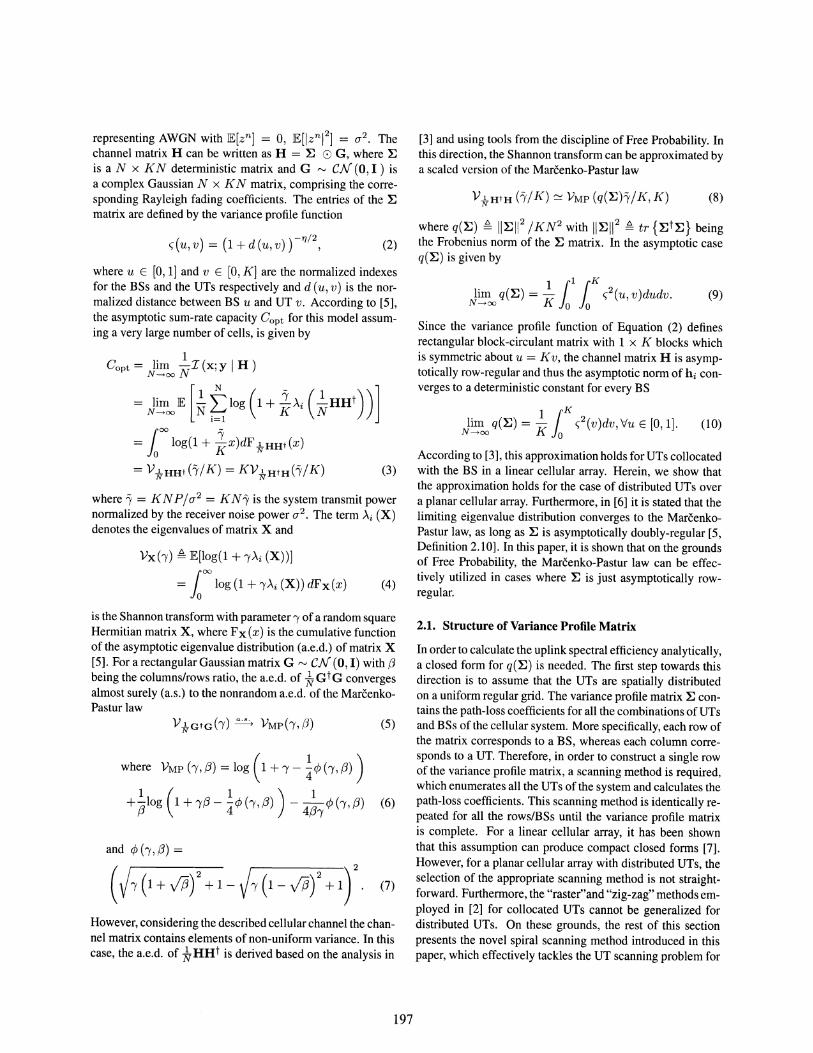
Fig. 1. Cell of interest (on the left) and cell of the mth tier ofinterference (on the right).

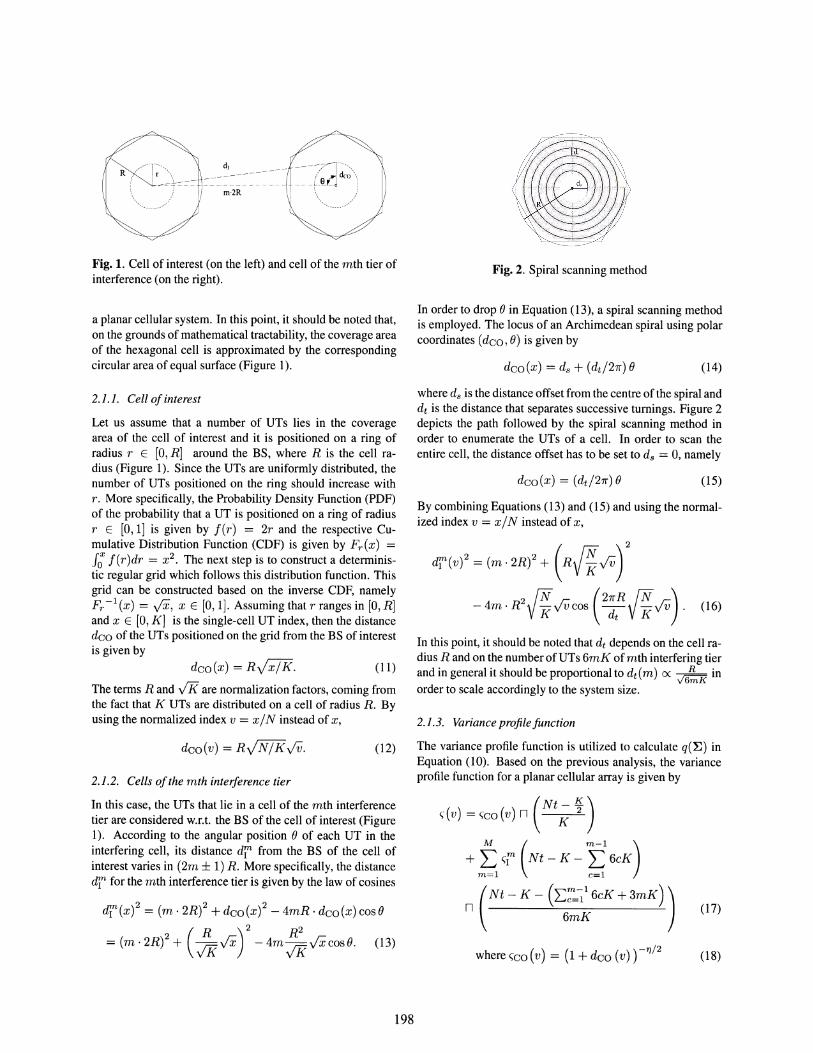
Fig. 2. Spiral scanning method

In order to drop () in Equation (13), a spiral scanning methodis employed. The locus of an Archimedean spiral using polarcoordinates (dco, ()) is given by

a planar cellular system. In this point, it should be noted that,on the grounds of mathematical tractability, the coverage areaof the hexagonal cell is approximated by the correspondingcircular area of equal surface (Figure 1). dco(x) = ds + (dt /21r) () (14)

The terms Rand JI( are normalization factors, coming fromthe fact that K UTs are distributed on a cell of radius R. Byusing the normalized index v = x / N instead of x,

dr(X)2 = (m . 2R)2 + dco (x)2 - 4mR . dco (x) cos ()

(R )2 R2

= (m· 2R)2 + JI(vX - 4m JI(vXcos B. (13)

2.1.2. Cells ofthe mth interference tier

In this case, the UTs that lie in a cell of the mth interferencetier are considered w.r.t. the BS of the cell of interest (Figure1). According to the angular position () of each UT in theinterfering cell, its distance dr from the BS of the cell ofinterest varies in (2m ± 1) R. More specifically, the distancedr for the mth interference tier is given by the law of cosines

(18)

(17)

(15)

(16)

dco(x) = (dt /21r) ()

where ~co (v) = (1 + dco (v) ) -7]/2

(Nt- K)~- (v) = ~co (v) n K 2

M ( m-l)+J;\} Nt-K- ~6CK

n (Nt - K- (L:~16cK+3mK))6mK

2.1.3. Variance profile function

The variance profile function is utilized to calculate q(~) inEquation (10). Based on the previous analysis, the varianceprofile function for a planar cellular array is given by

In this point, it should be noted that dt depends on the cell ra­dius R and on the number of UTs 6mK of mth interfering tierand in general it should be proportional to dt(m) (X v'6~K inorder to scale accordingly to the system size.

By combining Equations (13) and (15) and using the normal­ized index v = x / N instead of x,

where ds is the distance offset from the centre of the spiral anddt is the distance that separates successive turnings. Figure 2depicts the path followed by the spiral scanning method inorder to enumerate the UTs of a cell. In order to scan theentire cell, the distance offset has to be set to ds = 0, namely

(12)

(11)dco(x) = RJx/K.

dco(v) = RJN/Kv/V.

2.1.1. Cell of interest

Let us assume that a number of UTs lies in the coveragearea of the cell of interest and it is positioned on a ring ofradius r E [0, R] around the BS, where R is the cell ra­dius (Figure 1). Since the UTs are uniformly distributed, thenumber of UTs positioned on the ring should increase withr. More specifically, the Probability Density Function (PDF)of the probability that a UT is positioned on a ring of radiusr E [0,1] is given by f(r) = 2r and the respective Cu­mulative Distribution Function (CDF) is given by Fr (x) =foX f (r )dr = x2

• The next step is to construct a determinis­tic regular grid which follows this distribution function. Thisgrid can be constructed based on the inverse CDF, namelyFr-1(x) = VX, x E [0,1]. Assuming that r ranges in [O,R]and x E [0, K] is the single-cell UT index, then the distancedco of the UTs positioned on the grid from the BS of interestis given by

198

and ~I (v) = (1 + dI (v) ) -17/2

(19)

The reet functions are used in order to apply different vari­ance profile functions to UTs that belong to the cell of interestand to each of the M interfering tiers. The factor 6mK is dueto the fact that the mth interfering tier includes 6m cells andthus 6mK UTs, which can be treated equally on the groundsof symmetry.

3. USER DISTRIBUTION RESULTS

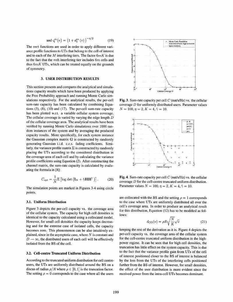
This section presents and compares the analytical and simula­tions capacity results which have been produced by applyingthe Free Probability approach and running Monte Carlo sim­ulations respectively. For the analytical results, the per-cellsum-rate capacity has been calculated by combining Equa­tions (3), (8), (10) and (17). The per-cell sum-rate capacityhas been plotted w.r.t. a variable cellular system coverage.The cellular coverage is varied by varying the edge length Dof the cellular coverage area. The analytical results have beenverified by running Monte Carlo simulations over 1000 ran­dom instances of the system and by averaging the producedcapacity results. More specifically, for each system instancethe Gaussian complex matrix G is constructed by randomlygenerating Gaussian i.i.d. c.c.s. fading coefficients. Simi­larly, the variance profile matrix E is constructed by randomlyplacing the UTs according to the considered distribution inthe coverage area of each cell and by calculating the varianceprofile coefficients using Equation (2). After constructing thechannel matrix, the sum-rate capacity is calculated by evalu­ating the formula in [8]:

Copt = ~E [log det (IN +iHHt )] . (20)

The simulation points are marked in Figures 3-4 using circlepoints.

o Monte Carlo SimulationMarcenko-Pastur Approximation

- Spiral Analysis

102

Cellular Coverage 0

Fig. 3. Sum-rate capacity per cell C (natls/Hz) vs. the cellularcoverage D for uniformly distributed users. Parameter valuesN = 100,17 = 2, K = 4, i = 10.

p~

p=O.OOIp=O.OIp=O.1

-p=l

102

Cellular Coverage D

Fig. 4. Sum-rate capacity per cell C (natls/Hz) vs. the cellularcoverage D for the cell-centre truncated uniform distribution.Parameter values N = 100, TJ = 2, K = 4, i = 10.

are collocated with the BS and the setting p = 1 correspondsto the case where UTs are uniformly distributed all over thecell's coverage area. In order to produce an analytical resultfor this distribution, Equation (12) has to be modified as fol­lows:

keeping the rest of the derivation as it is. Figure 4 depicts theper-cell capacity vs. the coverage area of the cellular systemfor the cell-centre truncated uniform distribution in the high­power regime. It can be seen that for high cell densities, thetruncation has little effect on the system capacity. This is dueto the fact that the variance profile gain from UTs of the cellof interest positioned closer to the BS of interest is balancedby the loss from the UTs of the interfering cells positionedfurther from the BS of interest. However, for small densities,the effect of the user distribution is more evident since thereceived power from the intra-cell UTs becomes dominant.

3.1. Uniform Distribution

Figure 3 depicts the per-cell capacity vs. the coverage areaof the cellular system. The capacity for high cell densities isidentical to the capacity calculated using a collocated model.However, for small cell densities the capacity keeps decreas­ing and for the extreme case of isolated cells, the capacitybecomes zero. This phenomenon can be also intuitively ex­plained, since in the asymptotic case, where N is constant andD -? 00, the distributed users of each cell will be effectivelyisolated from the BS of the cell.

3.2. Cell-centre Truncated Uniform Distribution

According to the truncated uniform distribution for cell centre­users, the UTs are uniformly distributed around the BS on adiscus of radius p/ R where p E [0, 1] is the truncation factor.The setting p = acorresponds to the case where all the users

199

dco(v) = PR.J!£.;v (21)

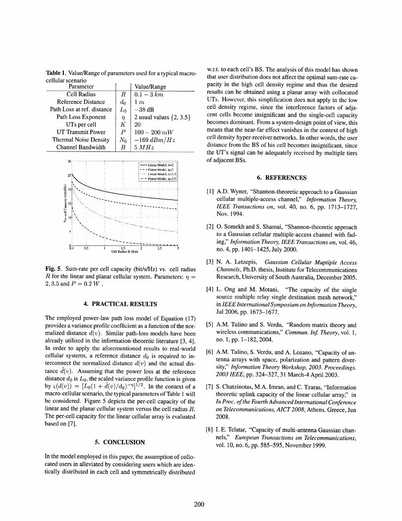
Table 1. Value/Range of parameters used for a typical macro­cellular scenario

Parameter Value/RangeCell Radius R 0.1- 3 km

Reference Distance do 1mPath Loss at ref. distance Lo -38dB

Path Loss Exponent 1] 2 usual values {2, 3.5}UTs per cell K 20

UT Transmit Power P 100 - 200mWThermal Noise Density No -169 dBm/Hz

Channel Bandwidth B 5 MHz

30

25

~,1

''',

0.5

................. .. ..,.-. .... ,-.-

1.5Cell Radius R (Km)

2.5

w.r.t. to each cell's BS. The analysis of this model has shownthat user distribution does not affect the optimal sum-rate ca­pacity in the high cell density regime and thus the desiredresults can be obtained using a planar array with collocatedUTs. However, this simplification does not apply in the lowcell density regime, since the interference factors of adja­cent cells become insignificant and the single-cell capacitybecomes dominant. From a system-design point of view, thismeans that the near-far effect vanishes in the context of highcell density hyper-receiver networks. In other words, the userdistance from the BS of his cell becomes insignificant, sincethe UT's signal can be adequately received by multiple tiersof adjacent BSs.

6. REFERENCES

[1] A.D. Wyner, "Shannon-theoretic approach to a Gaussiancellular multiple-access channel," Information Theory,IEEE Transactions on, vol. 40, no. 6, pp. 1713-1727,Nov. 1994.

[2] O. Somekh and S. Shamai, "Shannon-theoretic approachto a Gaussian cellular multiple-access channel with fad­ing," Information Theory, IEEE Transactions on, vol. 46,no. 4, pp. 1401-1425, July 2000.

Fig. 5. Sum-rate per cell capacity (bit/sIHz) vs. cell radiusR for the linear and planar cellular system. Parameters: r/ =2,3.5 and P = 0.2 W .

4. PRACTICAL RESULTS

The employed power-law path loss model of Equation (17)provides a variance profile coefficient as a function of the nor­malized distance d(v). Similar path-loss models have beenalready utilized in the information-theoretic literature [3, 4].In order to apply the aforementioned results to real-worldcellular systems, a reference distance do is required to in­terconnect the normalized distance d(v) and the actual dis­tance d(v). Assuming that the power loss at the referencedistance do is L o, the scaled variance profile function is givenby c;(d(v)) = [Lo(l + d(v)/do)-17]1/2. In the context of amacro-cellular scenario, the typical parameters ofTable 1 willbe considered. Figure 5 depicts the per-cell capacity of thelinear and the planar cellular system versus the cell radius R.The per-cell capacity for the linear cellular array is evaluatedbased on [7].

5. CONCLUSION

In the model employed in this paper, the assumption of collo­cated users in alleviated by considering users which are iden­tically distributed in each cell and symmetrically distributed

[3] N. A. Letzepis, Gaussian Cellular Muptiple AccessChannels, Ph.D. thesis, Institute for TelecommunicationsResearch, University of South Australia, December 2005.

[4] L. Ong and M. Motani, "The capacity of the singlesource multiple relay single destination mesh network,"in IEEE International Symposium on Information Theory,JuI2006,pp.1673-1677.

[5] A.M. Tulino and S. Verdu, "Random matrix theory andwireless communications," Commun. In! Theory, vol. 1,no. 1,pp. 1-182,2004.

[6] A.M. Tulino, S. Verdu, and A. Lozano, "Capacity of an­tenna arrays with space, polarization and pattern diver­sity," Information Theory Workshop, 2003. Proceedings.2003 IEEE, pp. 324-327,31 March-4 April 2003.

[7] S. Chatzinotas, M.A. Imran, and C. Tzaras, "Informationtheoretic uplink capacity of the linear cellular array," inIn Proc. ofthe Fourth AdvancedInternational Conferenceon Telecommunications, AICT 2008, Athens, Greece, Jun2008.

[8] I. E. Telatar, "Capacity of multi-antenna Gaussian chan­nels," European Transactions on Telecommunications,vol. 10, no. 6, pp. 585-595, November 1999.

200