L-invariants of low symmetric powers

of modular forms and Hida

deformations

Robert William Harron

A Dissertation

Presented to the Faculty

of Princeton University

in Candidacy for the Degree

of Doctor of Philosophy

Recommended for Acceptance

by the Department of

Mathematics

Adviser: Andrew Wiles

September 2009

c© Copyright by Robert William Harron, 2009.

All Rights Reserved

Abstract

We obtain formulae for Greenberg’s L-invariant of symmetric square and symmetric

sixth power motives attached to p-ordinary modular forms in the vein of theorem

3.18 of [GS93]. For the symmetric square of f , the formula obtained relates the L-

invariant to the derivative of the p-adic analytic function interpolating the pth Fourier

coefficient (equivalently, the unit root of Frobenius) in the Hida family attached to f .

We present a different proof than Hida’s, [Hi04], with slightly different assumptions.

The symmetric sixth power of f requires a bigger p-adic family. We take advantage of

a result of Ramakrishnan–Shahidi ([RS07]) on the symmetric cube lifting to GSp(4)/Q,

Hida families on the latter ([TU99] and [Hi02]), as well as results of several authors on

the Galois representations attached to automorphic representations of GSp(4)/Q, to

compute the L-invariant of the symmetric sixth power of f in terms of the derivatives

of the p-adic analytic functions interpolating the eigenvalues of Frobenius in a Hida

family on GSp(4)/Q. We must however impose stricter conditions on f in this case.

Here, Hida’s work (e.g. [Hi07]) does not provide answers as specific as ours.

In both cases, the method consists in using the big Galois deformations and some

multilinear algebra to construct global Galois cohomology classes in a fashion remi-

niscent of [Ri76]. The method employs explicit matrix computations.

iii

Contents

Abstract . . . . . . . . . . . . . . . . . . . . . . . . . . . . . . . . . . . . . iii

Introduction 1

Notation 5

1 Greenberg’s L-invariant 8

1.1 Basic setup . . . . . . . . . . . . . . . . . . . . . . . . . . . . . . . . 9

1.2 The exceptional subquotient . . . . . . . . . . . . . . . . . . . . . . . 10

1.3 Selmer groups . . . . . . . . . . . . . . . . . . . . . . . . . . . . . . . 13

1.4 Definition of the L-invariant . . . . . . . . . . . . . . . . . . . . . . . 19

1.5 Using a global Galois cohomology class . . . . . . . . . . . . . . . . . 24

2 L-invariant of the symmetric square of a modular form 26

2.1 The symmetric square Galois representation . . . . . . . . . . . . . . 27

2.2 The Hida deformation of ρf . . . . . . . . . . . . . . . . . . . . . . . 30

2.3 Computing the L-invariant . . . . . . . . . . . . . . . . . . . . . . . . 32

2.3.1 Obtaining a global Galois cohomology class . . . . . . . . . . 32

2.3.2 The L-invariant . . . . . . . . . . . . . . . . . . . . . . . . . . 36

2.4 Concluding remarks . . . . . . . . . . . . . . . . . . . . . . . . . . . . 40

3 L-invariant of the symmetric sixth power of a modular form 43

3.1 The symmetric power Galois representations . . . . . . . . . . . . . . 45

iv

3.1.1 Just enough on finite-dimensional representations of GL(2) . . 47

3.2 The symmetric cube lifting to GSp(4)/Q . . . . . . . . . . . . . . . . 47

3.3 The Hida deformation of ρ3 . . . . . . . . . . . . . . . . . . . . . . . 48

3.3.1 The Hida deformation . . . . . . . . . . . . . . . . . . . . . . 49

3.3.2 The GL(2) Hida family within . . . . . . . . . . . . . . . . . . 50

3.4 Computing the L-invariant . . . . . . . . . . . . . . . . . . . . . . . . 51

3.4.1 The multilinear algebra involved . . . . . . . . . . . . . . . . . 51

3.4.2 The computation . . . . . . . . . . . . . . . . . . . . . . . . . 54

3.4.3 Relation to the symmetric square L-invariant . . . . . . . . . 58

3.5 Concluding remarks . . . . . . . . . . . . . . . . . . . . . . . . . . . . 61

Bibliography 61

v

Introduction

In the mid 1980s, searching for a p-adic analogue of the Birch and Swinnerton-Dyer

conjecture, Mazur, Tate, and Teitelbaum ([MTT86]) discovered some exceptional be-

haviour occurring in the p-adic interpolation of L-functions of elliptic curves. Specifi-

cally, the p-adic L-function can vanish at s = 1 even when the archimedean L-function

does not. This phenomenon is called an “exceptional zero” (or “trivial zero”, as it

trivially arises from the vanishing of the interpolation factor). Based on numerical

computations, they conjectured that a certain p-adic quantity, the L-invariant, should

recuperate a non-trivial interpolation property relating the derivative of the p-adic

L-function to the archimedean L-function. This quantity was defined in terms of the

multiplicative p-adic period of the elliptic curve (i.e. the Tate period, q). They fur-

ther formulated a conjecture for higher weight modular forms that such an L-invariant

should depend only locally on E.

In the early 1990s, Greenberg and Stevens proved Mazur, Tate and Teitelbaum’s

conjecture ([GS93]) for modular elliptic curves and weight two modular forms. Their

clever method consists in adding a variable to the problem via the use of Hida families

(that is, p-adic analytic families of p-ordinary modular forms of varying weight). The

usual p-adic L-function can then be replaced by a two-variable p-adic L-function that

additionally interpolates values as the weight varies in the Hida family. The problem

is then broken into two pieces: the first is to relate the L-invariant to the derivative

of the two-variable p-adic L-function in the weight direction, the second, to use the

1

p-adic functional equation to transfer this result to the usual “cyclotomic” direction.

By reinterpreting the L-invariant in terms of Galois cohomology and infinitesimal de-

formations, Greenberg and Stevens obtain a key result in their proof, namely theorem

3.18 of [GS93] stating that the L-invariant of a weight two modular form, f , that has

an exceptional zero, is given by

L(f) = −2a′p (1)

where a′p is the derivative of the p-adic analytic function that interpolates the pth

Fourier coefficient, ap, (equivalently, the unit root of Frobenius) as the weight varies

in the Hida family. In this thesis, we prove analogues of this result. Note that

several more definitions of the L-invariant and proofs of the Mazur–Tate–Teitelbaum

conjecture have been given by other mathematicians; see Colmez’s article [Cz05] for

an overview.

Shortly thereafter, in [G94], Greenberg proposed a definition for the L-invariant

of rather general p-ordinary p-adic Galois representations to go along with the con-

jectures of Coates and Perrin-Riou concerning p-adic L-functions ([CoPR89, Co89]).

It is this version of the L-invariant that we treat in this thesis. In [G94, p. 170],

Greenberg treats the case of arbitrary symmetric powers of an elliptic curve with

split multiplicative reduction at p, and even symmetric powers of CM elliptic curves

with good, ordinary reduction at p. In both cases, he shows that the L-invariant is

independent of the power.

Subsequent work on Greenberg’s L-invariant of symmetric powers of ordinary

modular forms has mostly been done by Hida in a series of papers starting with [Hi04]

(see [Hi07] for the most up-to-date version of his work). His results rely on conjectures

concerning the local structure of the versal nearly ordinary Galois deformation ring

of the symmetric power Galois representations. Furthermore, for powers greater than

2

two, his formulae say very little about the case where the modular form has level

prime to p.

This thesis establishes formulae for the L-invariants of the symmetric square and

some symmetric sixth power ordinary modular forms. For the symmetric square,

Hida’s results are mostly complete. We include our work on the subject as the ap-

proach differs from Hida’s and does not require knowledge of the versal nearly ordinary

Galois deformation ring. The theorem we obtain is the following:

Theorem A. Let f be a p-ordinary, weight k0 ≥ 2, new, holomorphic eigenform

of character ψ (of conductor prime to p) and arbitrary level. Assume the balanced

Selmer group vanishes:

SelQ(Sym2ρf (1− k0)

)= 0.

Then,

L(Sym2ρf (1− k0)

)= −

2a′pap. (2)

For the symmetric sixth power, the Hida deformation of f on GL(2) is insuffi-

cient for our purposes. We take advantage of the symmetric cube lift to GSp(4)/Q

of Ramakrishnan–Shahidi in [RS07] and the work of Tilouine–Urban on Hida defor-

mations on GSp(4) ([TU99]). This requires extra conditions on the modular form f ,

but provides us with the following result of chapter 3:

Theorem B. Let f ∈ Sk0(Γ1(N)) be a p-ordinary, non-CM, even weight k0 ≥ 4 new

eigenform of level prime to p and trivial character. Suppose Sym3ρf is residually

absolutely irreducible. Assume the balanced Selmer group vanishes:

SelQ(Sym6ρf (3(1− k0))

)= 0,

and that the GSp(4) universal p-adic Hecke algebra is unramified over the Iwasawa

3

algebra at the prime corresponding to Sym3f . Then, for all but finitely many p

L (ρ6) = L(Sym6ρf (3(1− k0))

)= 3apa

(2,1)p − a3

pa(1,1)p , (3)

where a(i,1)p are derivatives of specific p-adic analytic functions interpolating eigenval-

ues of Frobenius in a certain Hida family on GSp(4).

In particular, we obtain a formula for the symmetric sixth power L-invariant when

f has level prime to p. We view such a result as encouraging evidence that further

instances of functoriality can be combined with Hida deformations on higher rank

groups to yield results on higher symmetric power L-invariants.

The symmetric sixth power L-invariant computation also yields the symmetric

square L-invariant. This allows us to compare the two in an attempt to verify if they

are equal — as is the case for CM elliptic curves. We fall slightly short of a conclusive

result, but at least obtain the following:

Theorem B′. In the situation of theorem B, we have that

L(ρ6) = −10a3pa

(1,1)p + 6L(ρ2). (4)

The results of this thesis lay groundwork for proving generalizations of the Mazur–

Tate–Teitelbaum conjecture. Furthermore, they suggest that higher symmetric pow-

ers could be addressed via new instances of functoriality — such as the very recent

potential automorphy results of [BLGHT09]. In [Hi07, p. 6], Hida mentions that

alternate methods of computing L-invariants could lead to a proof of [Hi07, Conjec-

ture 0.1]. That is, our results may be useful in studying the local structure of nearly

ordinary Galois deformation rings.

4

Notation

Let us record some common notation and nomenclature that we will use throughout

this thesis.

We fix throughout a rational prime p. Let K be a finite extension of Qp. Let GQ

denote the absolute Galois group of Q (relative to a fixed algebraic closure Q of Q).

Fix an embedding, ιp, of Q into a fixed algebraic closure K = Qp. This identifies

the absolute Galois group GQp of Qp with the decomposition group Gp ⊆ GQ of the

prime above p corresponding to ιp. Let Ip ⊆ Gp denote the inertia subgroup. Let

χp denote the p-adic cyclotomic character, and let K(1) denote the vector space K

with the Galois action given by χp. We denote the adeles of a global field F by AF ,

dropping the subscript for F = Q. The finite adeles will be denoted AF,f and the

infinite adeles, AF,∞.

For compatibility with [G94], we use Frobp to denote an arithmetic Frobenius at

p, and we normalize the local reciprocity map

rec : Q×p −→ GabQp

so that Frobp corresponds to p. We remark that under this normalization

χp(rec(u)) = u−1

for any principal unit u in Z×p .

5

All representations will be finite-dimensional vector spaces (or finite free modules).

Given a Galois representation on a K-vector space V , we will denote by V ∗ the Tate

dual of V defined by

V ∗ := HomK (V,K(1)) .

Given a field F with algebraic closure F , we denote its absolute Galois group

by GF . If M is a topological GF -module M , we will denote the continuous Galois

cohomology of GF with coefficients in M by

H i(F,M) := H i(GF ,M) .

Given a GF -submodule M ′ of M , and a class c ∈ H i(F,M), we let cmodM ′ denote

the image of c under the natural map

H i(F,M) −→ H i(F,M/M ′) .

Given a representation V of GQ and a place v of Q, we will denote resv the natural

restriction map

resv : H1(Q, V ) −→ H1(Qv, V ) .

Furthermore, given a class c ∈ H1(Q, V ), we will often denote its image under resv

by cv.

Given an algebraic number field1 F , a reductive algebraic group G over F , and

an automorphic representation π of G(AF ), we recall that π can be decomposed as a

restricted tensor product

π =⊗v

′πv

over the places v of F , where πv denotes an admissible representation of G(Fv), for

v finite, and an admissible (gv, Kv)-module, for v infinite, where gv is the real Lie

1An algebraic number field will always refer to a finite extension of Q.

6

algebra of G(Fv) and Kv is a maximal compact subgroup of G(Fv). We will denote

the finite part of π by πf and the infinite part by π∞.

7

Chapter 1

Greenberg’s L-invariant

In this chapter, we recall Greenberg’s theory of L-invariants associated to the phe-

nomenon of trivial zeroes of p-adic L-functions attached to p-ordinary motives (as

developed in [G94]). We present the theory “with coefficients”1 so that it is suited to

our use in later chapters.

Greenberg’s theory grows out of the Galois cohomological reinterpretation of the

Mazur–Tate–Teitelbaum L-invariant presented in section 3 of [GS93]. In that original

case, the L-invariant has a manifestly “local” definition2 that makes it easier to deal

with than the more general cases, two of which we attack in subsequent chapters.

The basic premise of our approach is introduced in section 1.5. The contents of the

other sections are as follows. Section 1.1 introduces the most basic notions of interest,

while section 1.2 provides some refinements related to the exceptional nature of the

p-adic Galois representations we are studying. Section 1.3 defines the ordinary and

balanced Selmer groups and describes the fundamental properties that we will need.

Then, section 1.4 gives Greenberg’s definition of the L-invariant.

1i.e. we consider Galois representations on a vector space over a finite extension K of Qp.2It only depends on the action of the decomposition group at p. This is true for any case of type

M (see section 1.2 for the definition).

8

1.1 Basic setup

Our basic object of study in this chapter will be a continuous representation

ρ : GQ −→ AutK(V )

on a finite-dimensional vector space V over the p-adic field K (endowed with the p-

adic topology) which we will refer to simply as a p-adic representation. A fundamental

condition we impose on this representation is that of ordinarity (see definition 1.1.1

below).3 In this chapter, we will also impose three conditions Greenberg calls (S),

(T), and (U) in [G94]. These three conditions are easily seen to be satisfied for the

situations we deal with in subsequent chapters. The goal of Greenberg’s theory is to

study a certain exceptional behaviour in the theory of p-adic interpolation of values

of L-functions. In particular, we will be interested in the value of the archimedean

L-function of V at the point s = 1, so we will assume that V is critical at s = 1 (in the

sense of Deligne, [D79]) and is exceptional (in the sense of [G94], see definition 1.2.3

below). Later, in order to define the L-invariant, we will require that a certain Selmer

group of V — the balanced Selmer group — vanishes. According to Greenberg’s

conjectures in [G94], this latter condition should be equivalent to the non-vanishing

of L(1, V ).

Let us now define the conditions we impose on V .

Definition 1.1.1. A p-adic representation (ρ, V ) is called ordinary if there exists an

exhaustive, separated, descending filtration {F iV }i∈Z of GQp-stable K-subspaces of V

such that the inertia subgroup, Ip, acts on the ith graded piece griV = F iV/F i+1V

via multiplication by χip.

3A recent preprint of Denis Benois ([Be09]) uses the theory of (ϕ,Γ)-modules to suggest a gen-eralization of Greenberg’s L-invariant with ordinarity replaced by semistability. We do not addressthis notion here.

9

Remark 1.1.2. a) In other words, we have

· · · ⊇ F i−1V ⊇ F iV ⊇ F i+1V ⊇ · · ·

with

(exhaustive): F iV = V for i� 0

(separated): F iV = 0 for i� 0

and each F iV is sent to itself under the action of GQp . Furthermore, for any σ ∈ Ip

and v ∈ F iV

ρ(σ)v ≡ χip(σ)v mod F i+1V.

b) It is common to denote

F+V := F 1V and F−V := F 0V.

The first two conditions that Greenberg introduces are the following:

(S) for all i ∈ Z, GQp acts semisimply on griV ;

(U) V has no GQp-subquotient isomorphic to a cristalline extension of K by K(1).4

Before defining the condition (T), we require a slightly finer understanding of the

structure of V as a GQp-representation which we explain in the following section.

1.2 The exceptional subquotient

In [G94], Greenberg isolates a certain subquotient W of V that is supposed to control

the behaviour of V with respect to the exceptional zeros of its p-adic L-function. For

4Such an extension is cristalline if, and only if, under the Kummer map, it comes from a unit(equivalently, if it is in the Bloch–Kato H1

f (Qp,K)). Morally, this case is excluded as the L-invariantshould be infinite (see, for example, Proposition 4.5.5(2) of [Em06] for the case of two-dimensionalV over Qp).

10

this reason, we refer to W as the exceptional subquotient of V . In this short section,

we describe its basic structure and state the condition (T) that we impose on V .

The definition of W basically relies on a slight refinement of the filtration on V

between steps 0 and 2. Specifically, we introduce F 00V and F 11V with

F 0V ⊇ F 00V ⊇ F 1V ⊇ F 11V ⊇ F 2V.

Definition 1.2.1.

a) Let F 00V be the maximal GQp-stable subspace of F 0V such that GQp acts triv-

ially on the quotient F 00V/F 1V .

b) Let F 11V be the minimal GQp-stable subspace of F 1V such that GQp acts by

multiplication by χp on the quotient F 1/F 11V .

c) Define the exceptional subquotient W of V as

W := F 00V/F 11V.

We denote

m0 := dimK F00V/F 1V and m1 := dimK F

1V/F 11V

so that we have the equality dimKW = m0 +m1.

Remark 1.2.2. Since the action of GQp on griV (−i) is unramified, we may consider

the action of Frobp on it. Packaging this information together for all i, we define a

polynomial

H(x) :=∏i∈Z

det(I − Frobp p

ix|gri(V )(−i)).

Then, under hypothesis (S), for i = 0, 1, mi is the multiplicity of pi as an inverse root

11

of H(x). The inverse roots of H(x) enter into the conjectural p-adic interpolation

properties of the critical values of L(s, V ) as stated in the work of Coates and Perrin-

Riou ([CoPR89, Co89]). This is the link that motivates the definition of W ; we refer

to the introduction of [G94] for the details.

The exceptional subquotient is an ordinary GQp-representation; indeed, it has a

two step filtration given by

F 0W = W = F 00V/F 11V

F 1W = F 1V/F 11V

F 2W = 0.

Let t0 := dimKWGQp and t1 := dimK(W ∗)GQp .5 We obtain two GQp-linear maps: an

injection ϕ0 : Kt0 ↪→ W and a surjection ϕ1 : W � K(1)t1 . Letting

M := ker(ϕ1)/ im(ϕ0),

we obtain an isomorphism of GQp-representations

W ∼= M ⊕Kt0 ⊕K(1)t1 .

The subspace M is a non-split extension of Kt by K(1)t for 2t = dimKW − t0 − t1.

A representation V with W ∼= M is said to be of type M . This is the case in the

original Greenberg–Stevens work in [GS93]; indeed, in their situation V = W is a

non-split extension of Qp by Qp(1). One of our goals in this work is to investigate

the case where V is not of this type. This requires an understanding of the global

Galois cohomology of V .6

5Recall that we use −∗ to denote the Tate dual HomK(−,K(1)).6See the discussion on pages 169–170 of [G94] for more details.

12

We may now state condition (T) as follows:

(T) At least one of t0 or t1 is zero.

Definition 1.2.3. An ordinary p-adic representation satisfying conditions (S), (T),

and (U) is called exceptional if its exceptional subquotient is non-zero. We define

e := t+ t0 + t1.

Then V is exceptional if, and only if, e 6= 0.

Greenberg conjectures that the order of vanishing of the p-adic L-function of V at

s = 1 is more than that of the archimedean L-function by e.

1.3 Selmer groups

Selmer groups for arbitrary ordinary p-adic Galois representations were introduced

by Greenberg in [G89] for the purpose of generalizing the main conjecture of Iwasawa

theory (and Mazur’s generalization of it to good, ordinary, modular elliptic curves,

[Mz72]). The Selmer groups he deals with in that paper are over the cyclotomic

Zp-extension Q∞/Q and are conjecturally related to the p-adic L-function of V . In

the last section of [G89], Greenberg suggests a possible definition for a Selmer group

over Q that should be related to the archimedean L-function of V . Trivial zero

considerations led Greenberg in [G94] to define a new Selmer group over Q (which

we follow Hida in calling the balanced Selmer group). In this section, we introduce

these Selmer groups and prove some basic properties that they satisfy. We expect

that everything here is known to the experts.

Recall that a Selmer group is defined by a collection of local conditions, i.e a

subspace Lv(V ) ⊆ H1(Qv, V ) for each place v of Q. For the Selmer groups we

13

consider, the conditions at v 6= p will always be

Lv(V ) = H1nr(Qv, V )

where

H1nr(Qv, V ) := ker

(H1(Qv, V ) −→ H1(Iv, V )

)= im

(H1(Gv/Iv, V

Iv)−→ H1(Qv, V )

)is the unramified part of H1(Qv, V ) (also called the space of unramified classes). At

p, several interesting conditions may be used. Given any such condition L?p(V ), the

associated Selmer group is defined as

Sel?Q (V ) := ker

H1(Q, V ) −→ H1(Qp, V ) /L?p(V )×

∏v-p

H1(Qv, V ) /Lv(V )

.

Remark 1.3.1. Given a GQ-stable lattice T in V and defining A := V/T , we may

define Selmer groups for T and A by the same formula, but using the local conditions

given by the inverse images (resp. the images) of those for V in T (resp. A).

The Selmer groups we are interested in are the following:

a) SelQ(V ), the ordinary Selmer group,

b) SelQ(V ), the balanced Selmer group.

The ordinary Selmer group (first introduced by Greenberg in [G89]) is defined

with respect to the local condition at p given by

Lp(V ) := ker(H1(Qp, V ) −→ H1

(Ip, V/F

+V)).

14

Remark 1.3.2. In [G94], Greenberg modified his definition over number fields slightly

to account for trivial zeroes; however, we follow Hida (e.g. [Hi-HMI]) and refer to the

modified Selmer group as the “balanced Selmer group”.

The local condition at p for the balanced Selmer group is defined as follows: it

consists of c ∈ H1(Qp, V ) such that

(Bal1) c ∈ ker (H1(Qp, V ) −→ H1(Qp, V/F00V )), and

(Bal2) cmodF 11V is in the image of

H1unit

(Qp, F

+V/F 11V)⊕H1

nr

(Qp, (F

00V/F 11V )Gp)

in H1(Qp, V/F11V ),

where H1unit(Qp, F

+V/F 11V ) ∼= H1unit(Qp, K(1)t+t1) ∼= H1

unit(Qp, K(1)) ⊗K Kt+t1 and

H1unit(Qp, K(1)) classifies cristalline extensions of K by K(1).7

The basic relation between these two Selmer groups is given by the following

lemma.

Lemma 1.3.3. At p,

Lp(V ) ⊂ Lp(V )

so

SelQ(V ) ⊆ SelQ(V ).

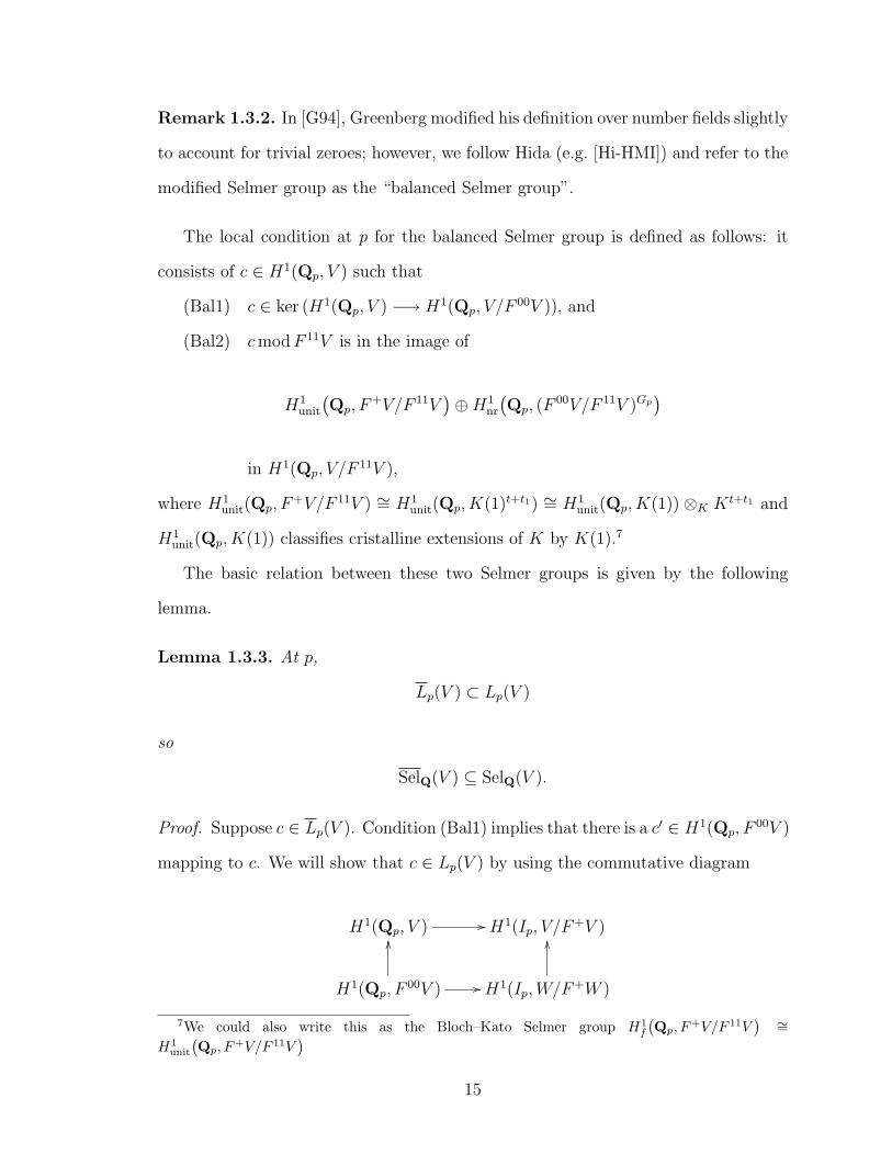
Proof. Suppose c ∈ Lp(V ). Condition (Bal1) implies that there is a c′ ∈ H1(Qp, F00V )

mapping to c. We will show that c ∈ Lp(V ) by using the commutative diagram

H1(Qp, V ) // H1(Ip, V/F+V )

H1(Qp, F00V )

OO

// H1(Ip,W/F+W )

OO

7We could also write this as the Bloch–Kato Selmer group H1f

(Qp, F

+V/F 11V) ∼=

H1unit

(Qp, F

+V/F 11V)

15

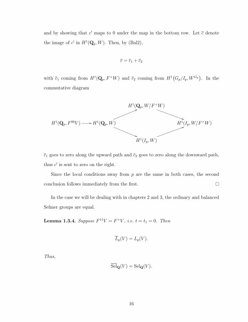
and by showing that c′ maps to 0 under the map in the bottom row. Let c denote

the image of c′ in H1(Qp,W ). Then, by (Bal2),

c = c1 + c2

with c1 coming from H1(Qp, F+W ) and c2 coming from H1

(Gp/Ip,W

Gp). In the

commutative diagram

H1(Qp,W/F+W )

))SSSSSSSSSSSSSSS

H1(Qp, F00V ) // H1(Qp,W )

66lllllllllllll

((RRRRRRRRRRRRRH1(Ip,W/F

+W )

H1(Ip,W )

55kkkkkkkkkkkkkkk

c1 goes to zero along the upward path and c2 goes to zero along the downward path,

thus c′ is sent to zero on the right.

Since the local conditions away from p are the same in both cases, the second

conclusion follows immediately from the first.

In the case we will be dealing with in chapters 2 and 3, the ordinary and balanced

Selmer groups are equal.

Lemma 1.3.4. Suppose F 11V = F+V , i.e. t = t1 = 0. Then

Lp(V ) = Lp(V ).

Thus,

SelQ(V ) = SelQ(V ).

16

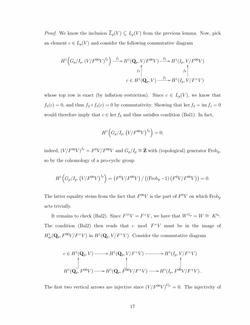
Proof. We know the inclusion Lp(V ) ⊆ Lp(V ) from the previous lemma. Now, pick

an element c ∈ Lp(V ) and consider the following commutative diagram

H1(Gp/Ip, (V/F

00V )Ip)

f1 // H1(Qp, V/F00V )

f2 // H1(Ip, V/F00V )

c ∈ H1(Qp, V )f5 //

f3

OO

H1(Ip, V/F+V )

f4

OO

whose top row is exact (by inflation–restriction). Since c ∈ Lp(V ), we know that

f5(c) = 0, and thus f2 ◦ f3(c) = 0 by commutativity. Showing that ker f2 = im f1 = 0

would therefore imply that c ∈ ker f3 and thus satisfies condition (Bal1). In fact,

H1(Gp/Ip,

(V/F 00V

)Ip)= 0;

indeed, (V/F 00V )Ip = F 0V/F 00V and Gp/Ip ∼= Z with (topological) generator Frobp,

so by the cohomology of a pro-cyclic group

H1(Gp/Ip,

(V/F 00V

)Ip)=(F 0V/F 00V

)/((Frobp−1)

(F 0V/F 00V

))= 0.

The latter equality stems from the fact that F 00V is the part of F 0V on which Frobp

acts trivially.

It remains to check (Bal2). Since F 11V = F+V , we have that WGp = W ∼= Kt0 .

The condition (Bal2) then reads that c mod F+V must be in the image of

H1nr(Qp, F

00V/F+V ) in H1(Qp, V/F+V ). Consider the commutative diagram

c ∈ H1(Qp, V ) // H1(Qp, V/F+V ) // H1(Ip, V/F

+V )

H1(Qp, F00V ) //

?�

OO

H1(Qp, F00V/F+V ) //?�

OO

H1(Ip, F00V/F+V ) .?�

OO

The first two vertical arrows are injective since (V/F 00V )Gp = 0. The injectivity of

17

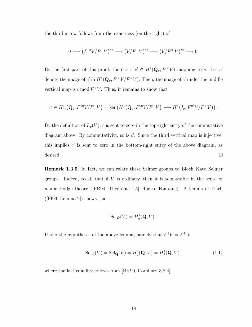
the third arrow follows from the exactness (on the right) of

0 −→(F 00V/F+V

)Ip −→ (V/F+V

)Ip −→ (V/F 00V

)Ip −→ 0.

By the first part of this proof, there is a c′ ∈ H1(Qp, F00V ) mapping to c. Let c′

denote the image of c′ in H1(Qp, F00V/F+V ). Then, the image of c′ under the middle

vertical map is cmodF+V . Thus, it remains to show that

c′ ∈ H1nr

(Qp, F

00V/F+V)

= ker(H1(Qp, F

00V/F+V)−→ H1

(Ip, F

00V/F+V)).

By the definition of Lp(V ), c is sent to zero in the top-right entry of the commutative

diagram above. By commutativity, so is c′. Since the third vertical map is injective,

this implies c′ is sent to zero in the bottom-right entry of the above diagram, as

desired.

Remark 1.3.5. In fact, we can relate these Selmer groups to Bloch–Kato Selmer

groups. Indeed, recall that if V is ordinary, then it is semi-stable in the sense of

p-adic Hodge theory ([PR94, Theoreme 1.5], due to Fontaine). A lemma of Flach

([Fl90, Lemma 2]) shows that

SelQ(V ) = H1g (Q, V ) .

Under the hypotheses of the above lemma, namely that F 1V = F 11V ,

SelQ(V ) = SelQ(V ) = H1g (Q, V ) = H1

f (Q, V ) , (1.1)

where the last equality follows from [BK90, Corollary 3.8.4].

18

Let us mention that if one were interested in replacing Q by a finite extension F ,

Pottharst has recently shown that

SelF (V ) = H1g (F, V )

(see [Po09] Theorem 3.5(2), Proposition 3.11(1), and example 3.13) so that the equa-

tions in (1.1) hold with Q replaced with F .

An important property of the balanced Selmer group — which gives it its name —

is the following result due to Greenberg. The proof relies on the criticality of L(s, V )

at s = 1 and, for this reason, we make this condition explicit in our statement.

Proposition 1.3.6 (Proposition 2 of [G94]). Assume V is critical at s = 1. Then

SelQ(V ) and SelQ(V ∗) have the same dimension.

1.4 Definition of the L-invariant

To define the L-invariant, Greenberg begins by isolating an e-dimensional subspace,

Hexcglob(V ), of a global Galois cohomology group. Taking its image, Hexc

loc (V ), in the

local cohomology with coefficients in W/F+W , he defines the L-invariant, L(V ), as

the “slope” of Hexcloc (V ) in certain natural coordinates. In this section, we give the

definitions of these objects, and in the next section, we outline a general idea for

computing the L-invariant in the case e = 1.

Recall that we are assuming that V is an ordinary p-adic Galois representation

satisfying conditions (S), (T), and (U), that is critical at s = 1 and exceptional. We

will now also be assuming that SelQ(V ) = 0.

19

Let us introduce a little bit of notation before continuing. For a group G acting

on V , we denote

F iH1(G, V ) := ker(H1(G, V ) −→ H1

(G, V/F iV

))= im

(H1(G,F iV

)−→ H1(G, V )

)with similar notations for F ii and W .

Let Σ be the set of primes ramified for V together with p and ∞, and let GΣ

denote Gal(QΣ/Q), where QΣ is the maximal extension of Q unramified outside of

Σ. From the local conditions that we have imposed away from p, it is clear that

SelQ(V ) ⊆ H1(GΣ, V ). Consider the beginning of the Poitou–Tate exact sequence

with local conditions Lv(V ):

0 −→ SelQ(V ) −→ H1(GΣ, V ) −→⊕v∈Σ

H1(Qv, V ) /Lv(V ) −→ SelQ(V ∗)

(see, for example, [PR00, Proposition A.3.3]). The vanishing of SelQ(V ), together

with proposition 1.3.6, thus gives an isomorphism

H1(GΣ, V ) −→⊕v∈Σ

H1(Qv, V ) /Lv(V ). (1.2)

We may exploit this isomorphism by defining an e-dimensional subspace of the right-

hand side, and transferring it over to the left. We use the following lemma.

Lemma 1.4.1. The subspace Lp(V ) has codimension e in F 00H1(Qp, V ).

For the proof, see [G94, p. 161].

Definition 1.4.2. Define Hexcglob(V ) to be the e-dimensional subspace of H1(GΣ, V )

corresponding to the subspace F 00H1(Qp, V ) /Lp(V ) of⊕

v∈Σ H1(Qv, V ) /Lv(V ) un-

der the isomorphism in (1.2).

20

Remark 1.4.3. In [G94], Greenberg uses the notation T for this subspace, whereas

Hida uses the notation H (see, for example, [Hi07]). Our notation attempts to convey

the sense that this subspace is a space of global cohomology classes attached to the

exceptional nature of V . Hopefully it is not too cumbersome.

Since we are assuming that V satisfies hypothesis (T), we will assume that in fact

t1 = 0 (as will be the case in the following chapters); otherwise, one can replace V

with V ∗. Consider the image of Hexcglob(V ) under the composition

λ : H1(GΣ, V ) −→ H1(Qp, V ) −→ H1(Qp, V/F

+V)

and note that the natural map

H1(Qp,W/F

+W)↪→ H1

(Qp, V/F

+V)

is an injection (indeed, H0(Qp, V/F00V ) = 0). We identify H1(Qp,W/F

+W ) with

its image inside H1(Qp, V/F+V ).

Proposition-Definition 1.4.4. The image of Hexcglob(V ) under λ satisfies the follow-

ing three properties:

a) λ(Hexcglob(V )) ⊆ H1(Qp,W/F

+W ),

b) dimλ(Hexcglob(V )) = e, and

c) λ(Hexcglob(V )) ∩H1

nr(Qp,W/F+W ) = 0.

We define Hexcloc (V ) to be λ(Hexc

glob(V )) considered as a subspace of H1(Qp,W/F+W ).

We refer to section 3 of [G94] for these statements.

21

One last step before defining the L-invariant is to discuss the natural coordinates

mentioned at the beginning of this section. The space W/F+W is a trivial GQp-

module, so

H1(Qp,W/F

+W) ∼= Hom

(GQp ,W/F

+W).

Any such homomorphism factors through the maximal pro-p quotient of GabQp

given by

Gal(F∞/Qp), where F∞ is the compositum of two Zp-extensions of Qp: the cyclotomic

one, Q∞,p, and the maximal unramified abelian extension Qnrp . Writing

Γ∞ := Gal (Q∞,p/Qp) ∼= Gal(F∞/Q

nrp

)and

Γnr := Gal(Qnrp /Qp

) ∼= Gal (F∞/Q∞,p) ,

we have that

Gal (F∞/Qp) = Γ∞ × Γnr.

Thus,

H1(Qp,W/F

+W)

= Hom(Γ∞,W/F

+W)× Hom

(Γnr,W/F

+W).

Let pr∞ and prnr denote the associated projections, let pr′∞ and pr′nr denote their

restrictions to Hexcloc (V ), and note that, by part c) of the above proposition-definition,

pr′∞ is invertible. The one-dimensional Qp-vector spaces Hom(Γ∞,Qp) and

Hom(Γnr,Qp) each have a natural basis given by the p-adic logarithm of the cy-

clotomic character, logχp, and the ord function (sending Frobp to 1), respectively.

Since

Hom(Γ∞,W/F+W ) = Hom(Γ∞,Qp)⊗W/F+W

22

and

Hom(Γnr,W/F+W ) = Hom(Γnr,Qp)⊗W/F+W,

logχp and ord define isomorphisms

ι∞ : Hom(Γ∞,W/F+W ) → W/F+W

logχp ⊗ w 7→ w

and

ιnr : Hom(Γnr,W/F+W ) → W/F+W

ord⊗w 7→ w.

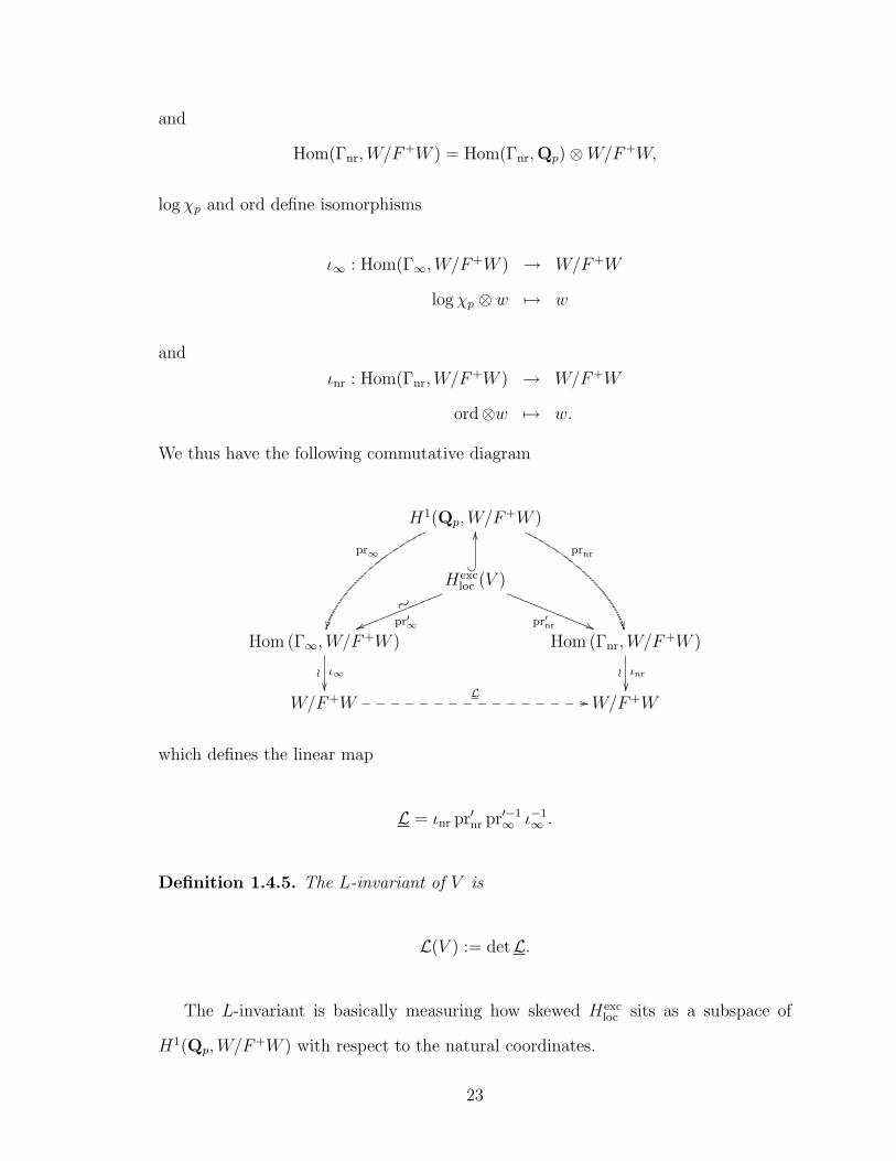
We thus have the following commutative diagram

H1(Qp,W/F+W )

pr∞

��

prnr

��

Hexcloc (V )

pr′∞

∼vvlllllllllllll

pr′nr ((RRRRRRRRRRRRR

?�

OO

Hom (Γ∞,W/F+W )

o ι∞��

Hom (Γnr,W/F+W )

o ιnr

��W/F+W

L //________________ W/F+W

which defines the linear map

L = ιnr pr′nr pr′−1∞ ι−1

∞ .

Definition 1.4.5. The L-invariant of V is

L(V ) := detL.

The L-invariant is basically measuring how skewed Hexcloc sits as a subspace of

H1(Qp,W/F+W ) with respect to the natural coordinates.

23

1.5 Using a global Galois cohomology class

This section is basically an extended remark discussing how one can compute the

L-invariant of a p-adic Galois representation with t0 = 1 and t = t1 = 0 starting with

a global Galois cohomology class.

Suppose that t0 = 1 and t = t1 = 0, and that we have somehow obtained [c] ∈

H1(Q, V ). Suppose further that [c] satisfies

a) [cv] ∈ H1nr(Qv, V ), for all v ∈ Σ \ {p},

b) [cp] ∈ F 00H1(Qp, V ),

c) [cp] 6≡ 0 modF+V .

Then, [c] generates Hexcglob. Thus, [cp] := ([cp] modF+V ) generates Hexc

loc . Since

W/F+W ∼= K, we may view the maps ι∞ pr∞ and ιnr prnr as giving K-coordinates on

H1(Qp,W/F+W ). If we have a cocycle representative cp of [cp] whose image lies in

F 00V/F+V — such a representative exists by condition b) — then we can explicitly

realize these coordinates as evaluation maps as follows. Let ϕ ∈ Hom(GQp ,W/F+W ).

Suppose prnr ϕ = y ord, then

ιnr prnr ϕ = y = y ord(Frobp) = ϕ(Frobp),

so the second coordinate is obtained by evaluating at Frobp. The first coordinate is

only slightly more complicated. Suppose pr∞ ϕ = x logχp. Let u be any principal

unit, so that χp(rec(u)) = u−1. Then

ι∞ pr∞ ϕ = x = − x

log ulogχp(rec(u)) = − 1

log uϕ(rec(u)).

24

Therefore, the coordinates of [cp] are

(− 1

log ucp(rec(u)), cp(Frobp)

)(1.3)

and the linear map L acts by scalar multiplication by the ratio of the second coor-

dinate to the first. In other words, the L-invariant is simply the slope of the line

generated by [cp]:

L(V ) =−cp(Frobp)1

log ucp(rec(u))

(1.4)

independent of the choice of principal unit u.

25

Chapter 2

L-invariant of the symmetric

square of a modular form

In this chapter, we prove a formula for Greenberg’s L-invariant of the symmetric

square of a p-ordinary elliptic modular form, f , only assuming that its balanced

Selmer group vanishes (corollary 2.3.5, also known as theorem A). The first results

on these L-invariants were those of Greenberg concerning Tate curves, and good

ordinary CM elliptic curves ([G94, p. 170]). Since then Hida has provided in [Hi04]

a conditional proof (known to be true in most cases) of the formula we prove in

this chapter relating the L-invariant to the p-adic analytic function interpolating the

eigenvalues of Frobenius in the Hida family attached to f . Our approach differs

from Hida’s in two important ways. Firstly, it does not require the existence of

the versal nearly p-ordinary Galois deformation ring, nor any knowledge of its local

structure. We also do not require the module of differentials he uses to carry out his

computations. For these reasons, we believe our proof to be of interest.

The difficult case of our theorem occurs when p does not divide the level of f

(the simpler case being the result of Greenberg on Tate curves). In this case, the

L-invariant is of a different nature than both the Tate curve case and the Greenberg–

26

Stevens result ([GS93]). Specifically, in those cases, the L-invariant is defined in terms

of local Galois cohomology groups, and techniques of Kummer theory and local Tate

duality suffice to arrive at an answer. In the case of a p-unramified modular form, a

global Galois cohomology class is required to compute the L-invariant. It is here that

we take inspiration from Ribet [Ri76] and seek out an irreducible Galois deformation

which becomes reducible at our point of interest. Specifically, we tensor the Hida

deformation with the constant deformation and study the family obtained.

In view of Greenberg’s result for Tate curves, we may restrict ourselves to the case

where p does not divide the level. In section 2.1, we describe the symmetric square

Galois representation and its exceptional subquotient. What little information we

require regarding the Hida deformation is contained in section 2.2. In section 2.3, we

present our computation of the L-invariant by first describing how we obtain a global

Galois cohomology class, then computing its local coordinates as in section 1.5. We

finish up this chapter with a short discussion of the questions not addressed in this

work, followed by other concluding remarks.

2.1 The symmetric square Galois representation

Let f ∈ Sk0(Γ0(N), ψ) be a p-ordinary, weight k0 ≥ 2 new eigenform of level N

(prime to p) and character ψ (of conductor prime to p). To ensure the vanishing of

the balanced Selmer group, one may make additional assumptions (see theorem 2.1.1

and the remark following it). Write αp for the unit root of the Hecke polynomial of f

at p and βp for the other root. Let E := Q(f) be the number field generated by the

Fourier coefficients of f . Let p|p be the prime of E determined by the embedding ιp

and let

ρf : GQ −→ GL(Vf )

27

be the contragredient1 of the p-adic Galois representation attached to f by Deligne

([D71]) on a two-dimensional Ep-vector space Vf .

Wiles showed ([W88, Theorem 2.1.4]) that

ρf |GQp∼

χk0−1p δ−1 ϕ

0 δ

(2.1)

where χp is the p-adic cyclotomic character and δ is the unramified character sending

Frobp to αp. The symmetric square of ρf |GQpis then equivalent to

χ

2(k0−1)p δ−2 2χk0−1

p ϕδ−1 ϕ2

χk0−1p ϕδ

δ2

.

Let ρ :=(Sym2ρf

)(1− k0) and denote its representation space by V . Then

ρ|GQp∼

χk0−1p δ−2 2ϕδ−1 χ1−k0

p ϕ2

1 χ1−k0p ϕδ

χ1−k0p δ2

. (2.2)

1For example, we take the Tate module of an elliptic curve, not its first etale cohomology group.

28

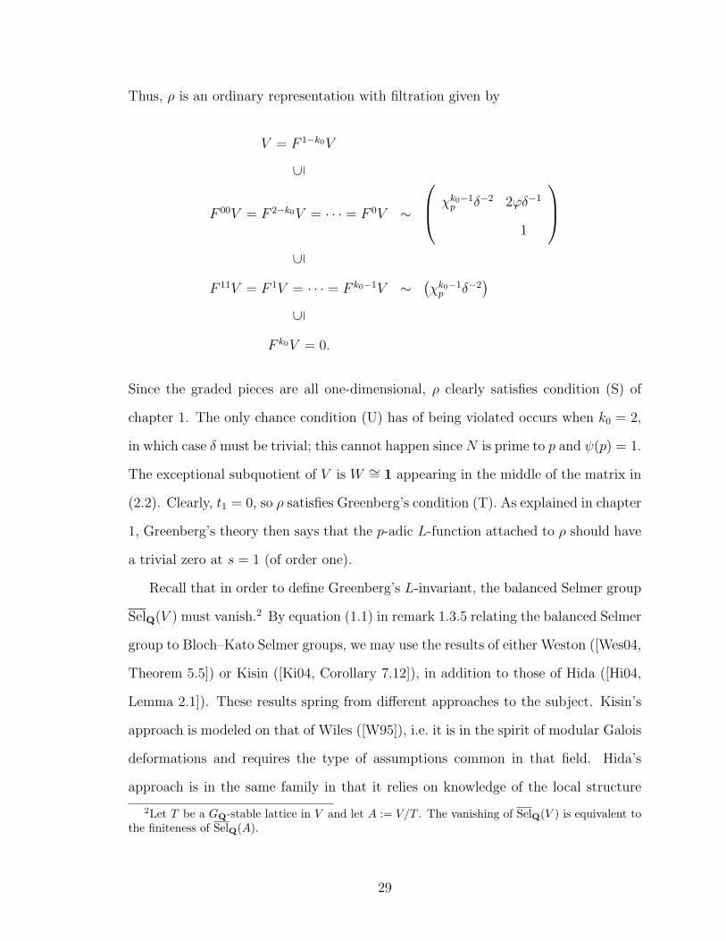
Thus, ρ is an ordinary representation with filtration given by

V = F 1−k0V

⊆

F 00V = F 2−k0V = · · · = F 0V ∼

χk0−1p δ−2 2ϕδ−1

1

⊆F 11V = F 1V = · · · = F k0−1V ∼

(χk0−1p δ−2

)⊆

F k0V = 0.

Since the graded pieces are all one-dimensional, ρ clearly satisfies condition (S) of

chapter 1. The only chance condition (U) has of being violated occurs when k0 = 2,

in which case δ must be trivial; this cannot happen since N is prime to p and ψ(p) = 1.

The exceptional subquotient of V is W ∼= 1 appearing in the middle of the matrix in

(2.2). Clearly, t1 = 0, so ρ satisfies Greenberg’s condition (T). As explained in chapter

1, Greenberg’s theory then says that the p-adic L-function attached to ρ should have

a trivial zero at s = 1 (of order one).

Recall that in order to define Greenberg’s L-invariant, the balanced Selmer group

SelQ(V ) must vanish.2 By equation (1.1) in remark 1.3.5 relating the balanced Selmer

group to Bloch–Kato Selmer groups, we may use the results of either Weston ([Wes04,

Theorem 5.5]) or Kisin ([Ki04, Corollary 7.12]), in addition to those of Hida ([Hi04,

Lemma 2.1]). These results spring from different approaches to the subject. Kisin’s

approach is modeled on that of Wiles ([W95]), i.e. it is in the spirit of modular Galois

deformations and requires the type of assumptions common in that field. Hida’s

approach is in the same family in that it relies on knowledge of the local structure

2Let T be a GQ-stable lattice in V and let A := V/T . The vanishing of SelQ(V ) is equivalent tothe finiteness of SelQ(A).

29

of the universal p-nearly ordinary Galois deformation ring that can be obtained from

modularity theorems. Weston’s approach is via geometric Euler systems and, with

some work, should apply to large classes of adjoint motives (such as those dealt with

in the next chapter). Let us combine these results.

Theorem 2.1.1 ([Hi04, Ki04, Wes04]). Let ρf denote a reduction of ρf modulo p.

Suppose at least one of the following holds

a) for any quadratic extension L/Q contained in Q(ζp3), ρf |GLis absolutely irre-

ducible;

b) ρf is not absolutely irreducible, and the diagonal characters of ρf ⊗ Fp are

distinct when restricted to GQ(ζp∞ );

c) f is special or supercuspidal at all primes dividing N , non-CM, (and p - N);

d) f satisfies the assumptions in theorem 1 of [Hi04].

Then, SelQ(V ) vanishes.

Remark 2.1.2. Conditions a) and b) are due to Kisin, condition c) is due to Weston,

and the last condition is due to Hida. Weston remarks that one should be able to

remove the assumptions on the ramification of f away from p via a more careful anal-

ysis of the bad reduction of the self-product of the Kuga–Sato variety. We entertain

hopes of addressing this question in future work.

2.2 The Hida deformation of ρf

To put f in a p-adic analytic family, we must replace it with its p-stabilization fp

given by

fp(z) = f(z)− βpf(pz);

30

in some sense, this “removes” the Euler factor corresponding to βp.3 Writing the

q-expansion of fp as

fp(q) =∑n≥1

anqn

one has

ap = αp.

By Hida theory, there exists an open disk U around k0 ∈ Zp and a formal q-expansion

that we denote

F =∑n≥1

αn(k)qn ∈ AUJqK

(where AU denotes the ring of p-adic analytic functions in the variable k ∈ U) such

that when k ∈ U is an integer greater than 1, the specialization Fk is the q-expansion

of a (non-zero) weight k, p-stabilized, p-ordinary newform of tame conductor N .

Furthermore, at k0, we have

Fk0 = fp.

The latter justifies the notation for αn(k) since αp(k0) = ap = αp.

Hida showed ([Hi86], [GS93, pp. 418–419]) that F gives rise to a “big” Galois

representation

ρF : GQ → GL(2,AU)

whose specialization at a given integer k ≥ 2 in U is equivalent to the contragredient

of that attached by Deligne to the modular form Fk. Moreover, Wiles [W88, Theo-

rem 2.2.2] (building on work of Mazur–Wiles [MzW86]) showed that the local Galois

representation

ρF |GQp: GQp → GL(2,AU)

3For an introduction to this operation, also known as a refinement, see [Mz00].

31

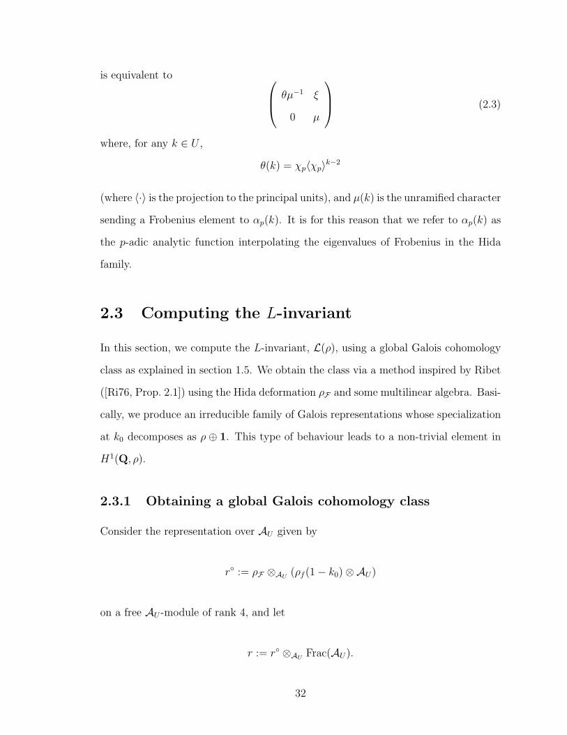
is equivalent to θµ−1 ξ

0 µ

(2.3)

where, for any k ∈ U ,

θ(k) = χp〈χp〉k−2

(where 〈·〉 is the projection to the principal units), and µ(k) is the unramified character

sending a Frobenius element to αp(k). It is for this reason that we refer to αp(k) as

the p-adic analytic function interpolating the eigenvalues of Frobenius in the Hida

family.

2.3 Computing the L-invariant

In this section, we compute the L-invariant, L(ρ), using a global Galois cohomology

class as explained in section 1.5. We obtain the class via a method inspired by Ribet

([Ri76, Prop. 2.1]) using the Hida deformation ρF and some multilinear algebra. Basi-

cally, we produce an irreducible family of Galois representations whose specialization

at k0 decomposes as ρ ⊕ 1. This type of behaviour leads to a non-trivial element in

H1(Q, ρ).

2.3.1 Obtaining a global Galois cohomology class

Consider the representation over AU given by

r◦ := ρF ⊗AU(ρf (1− k0)⊗AU)

on a free AU -module of rank 4, and let

r := r◦ ⊗AUFrac(AU).

32

Since ρ∨f∼= ρf (1− k0), specializing at k0 gives

r◦k0∼= ρf ⊗ ρ∨f ∼= End(ρf ) ∼= ρ⊕ 1

So we see that r has reducible reduction. It will in fact be a corollary of our method

that the representation r is irreducible (though one can easily prove this directly in

the non-CM case).

From the reducibility above, we construct a non-split extension of 1 by ρ, i.e. a

non-zero element of H1(Q, ρ). The method basically consists in scaling part of the

lattice by (s− k0). The explicit calculations are as follows.

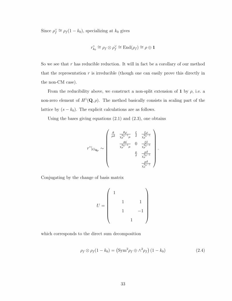
Using the bases giving equations (2.1) and (2.3), one obtains

r◦|GQp∼

θµδ

θϕ

χk0−1p µ

ξδ

ξϕ

χk0−1p

θδ

χk0−1p µ

0 ξδ

χk0−1p

µδ

µδ

χk0−1p

µδ

χk0−1p

.

Conjugating by the change of basis matrix

U =

1

1 1

1 −1

1

which corresponds to the direct sum decomposition

ρf ⊗ ρf (1− k0) =(Sym2ρf ⊕ ∧2ρf

)(1− k0) (2.4)

33

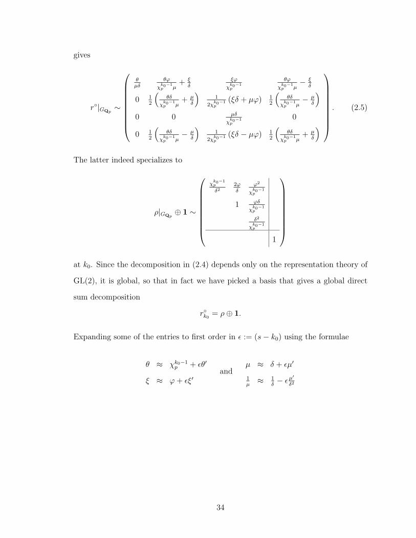
gives

r◦|GQp∼

θµδ

θϕ

χk0−1p µ

+ ξδ

ξϕ

χk0−1p

θϕ

χk0−1p µ

− ξδ

0 12

(θδ

χk0−1p µ

+ µδ

)1

2χk0−1p

(ξδ + µϕ) 12

(θδ

χk0−1p µ

− µδ

)0 0 µδ

χk0−1p

0

0 12

(θδ

χk0−1p µ

− µδ

)1

2χk0−1p

(ξδ − µϕ) 12

(θδ

χk0−1p µ

+ µδ

)

. (2.5)

The latter indeed specializes to

ρ|GQp⊕ 1 ∼

χk0−1p

δ22ϕδ

ϕ2

χk0−1p

1 ϕδ

χk0−1p

δ2

χk0−1p

1

at k0. Since the decomposition in (2.4) depends only on the representation theory of

GL(2), it is global, so that in fact we have picked a basis that gives a global direct

sum decomposition

r◦k0 = ρ⊕ 1.

Expanding some of the entries to first order in ε := (s− k0) using the formulae

θ ≈ χk0−1p + εθ′

ξ ≈ ϕ+ εξ′and

µ ≈ δ + εµ′

1µ≈ 1

δ− εµ′

δ2

34

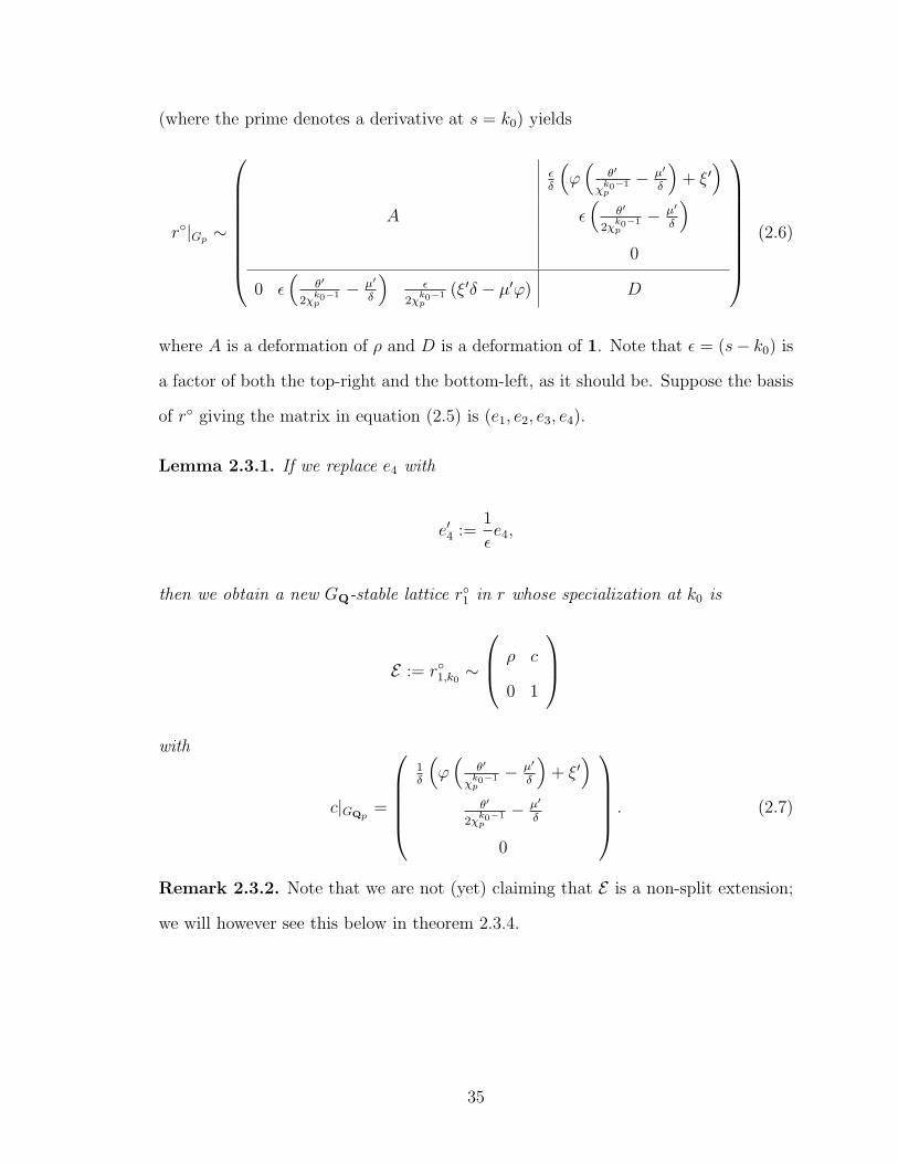
(where the prime denotes a derivative at s = k0) yields

r◦|Gp ∼

εδ

(ϕ(

θ′

χk0−1p

− µ′

δ

)+ ξ′

)A ε

(θ′

2χk0−1p

− µ′

δ

)0

0 ε(

θ′

2χk0−1p

− µ′

δ

)ε

2χk0−1p

(ξ′δ − µ′ϕ) D

(2.6)

where A is a deformation of ρ and D is a deformation of 1. Note that ε = (s− k0) is

a factor of both the top-right and the bottom-left, as it should be. Suppose the basis

of r◦ giving the matrix in equation (2.5) is (e1, e2, e3, e4).

Lemma 2.3.1. If we replace e4 with

e′4 :=1

εe4,

then we obtain a new GQ-stable lattice r◦1 in r whose specialization at k0 is

E := r◦1,k0 ∼

ρ c

0 1

with

c|GQp=

1δ

(ϕ(

θ′

χk0−1p

− µ′

δ

)+ ξ′

)θ′

2χk0−1p

− µ′

δ

0

. (2.7)

Remark 2.3.2. Note that we are not (yet) claiming that E is a non-split extension;

we will however see this below in theorem 2.3.4.

35

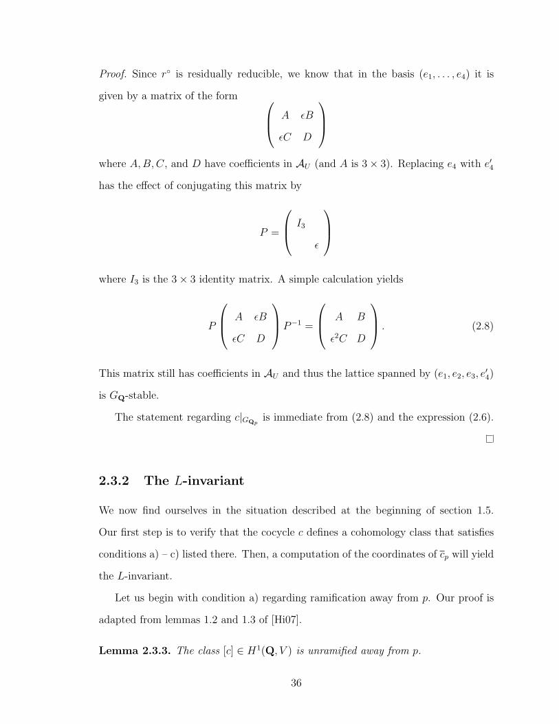
Proof. Since r◦ is residually reducible, we know that in the basis (e1, . . . , e4) it is

given by a matrix of the form A εB

εC D

where A,B,C, and D have coefficients in AU (and A is 3× 3). Replacing e4 with e′4

has the effect of conjugating this matrix by

P =

I3

ε

where I3 is the 3× 3 identity matrix. A simple calculation yields

P

A εB

εC D

P−1 =

A B

ε2C D

. (2.8)

This matrix still has coefficients in AU and thus the lattice spanned by (e1, e2, e3, e′4)

is GQ-stable.

The statement regarding c|GQpis immediate from (2.8) and the expression (2.6).

2.3.2 The L-invariant

We now find ourselves in the situation described at the beginning of section 1.5.

Our first step is to verify that the cocycle c defines a cohomology class that satisfies

conditions a) – c) listed there. Then, a computation of the coordinates of cp will yield

the L-invariant.

Let us begin with condition a) regarding ramification away from p. Our proof is

adapted from lemmas 1.2 and 1.3 of [Hi07].

Lemma 2.3.3. The class [c] ∈ H1(Q, V ) is unramified away from p.

36

Proof. Let q 6= p be a prime where ρ is ramified. The proof breaks into two parts

according to whether ρf is potentially unramified or potentially multiplicative at q.

Case 1): ρf potentially unramified at q. The representation ρ is then also poten-

tially unramified. Let L/Qq be a finite Galois extension such that the inertia group

of L, IL, acts trivially on ρ. Since Iq/IL is a finite group and ρ is an Ep-vector space

H1(Iq/IL, ρ) = 0.

The inflation–restriction exact sequence of Gq/Iq-modules yields

0 −→ H1(Iq, ρ) −→ H1(IL, ρ)Iq/IL .

Therefore, if we can show that c becomes zero in H1(IL, ρ), then c is unramified at

q. By definition, ρ is a trivial IL-module, so

H1(IL, ρ)Iq/IL = HomIq/IL(IL, ρ) = HomIq/IL(Zp(1), ρ).

The second equality holds because every homomorphism must factor through the

maximal pro-p quotient of IL. Note that since c passes through H1(Gq, ρ) on its

way to HomIq/IL(Zp(1), ρ), its image in the latter actually lies in HomGq/IL(Zp(1), ρ),

i.e. it gives a Frobq-equivariant map. Recall that Frobq acts by multiplication by q on

Zp(1). Its action on ρ is determined by its action on ρf and a Tate twist by (1− k0).

Specifically, the eigenvalues of Frobq on ρf , denoted λ1, λ2, are Weil numbers with

|λi| = qk0−1

2 ,

so the eigenvalues of Frobq on ρ are

λ2−j1 λj2q

1−k0 , for j = 0, 1, 2

37

all of which have absolute value 1. Equivariance implies that, for each z ∈ Zp(1),

qc(z) = c(qz) = c(Frobq z) = Frobq c(z) = λc(z)

where |λ| = 1 6= |q|. This is a contradiction. Hence, c must be zero in H1(Iq, V ).

Case 2): ρf potentially multiplicative at q. Its restriction to the decomposition

group at q is

ρf |Gq ∼

ηχk0−1p ησ

0 η

and

ρF |Gq ∼

νθ ντ

0 ν

.

Going through the matrix computations that give c shows that

cq =

η2(σθ′ − χk0−1

p τ ′)

η2θ′

2

0

. (2.9)

Since ρF is a Hida deformation, it satisfies conditions (K11–4) on page 4 of [Hi07].

The proof of lemma 1.3 of [Hi07] then shows that ρF |Iq is constant. This shows that

cq = 0 since every term in equation (2.9) has a derivative in it.

Condition b) of section 1.5 is simply that the third component of cp in (2.7) is

zero. Condition c) that cp is non-zero in H1(GQp ,W

) ∼= Hom(GQp ,Qp

)follows from

the following theorem.

Theorem 2.3.4. The coordinates of cp, discussed in section 1.5, are

(1

2,−µ

′(k0)(Frobp)

ap

). (2.10)

38

Since the first coordinate is non-zero,

• [c] is a non-zero cohomology class, and

• E is a non-split extension.

Since ap = µ(k0)(Frobp), we suggestively denote a′p := µ′(k0)(Frobp). From the

formula (1.4) for the L-invariant, the main theorem of this chapter is an immediate

corollary of the above theorem.

Corollary 2.3.5 (Theorem A). Let f be a p-ordinary, weight k0 ≥ 2, new, holomor-

phic eigenform of character ψ (of conductor prime to p) and arbitrary level. Assume

SelQ(Sym2ρf (1− k0)

)= 0. Then,

L(ρ) = L(Sym2ρf (1− k0)

)= −

2a′pap. (2.11)

Recall that, by theorem 2.1.1 and remark 2.1.2, the assumption on the vanishing

of the balanced Selmer group is known in many cases, and is expected in all cases.

Also, note that by the ordinarity assumption the order to which p divides the level is

less than or equal to one. In the case where p divides the level, the weight must be

two and this result is due to Greenberg [G94, p. 170].

It remains to prove theorem 2.3.4. We begin with a lemma.

Lemma 2.3.6. Let k ∈ U be an integer greater than or equal to 2, then, for any

principal unit u,

1) θ′(k)(Frobp) = 0 (2.12)

2)θ′(k)(rec(u))

χk−1(rec(u))= − log u. (2.13)

Proof. Recall that

θ(k) = χk−1p .

39

The first conclusion follows from the fact that χp(Frobp) = 1. The second conclusion

is a formula for the logarithmic derivative of θ at k. Recall that χp(rec(u)) = u−1, so

that

θ(k)(rec(u)) = u1−k.

Thus, its logarithmic derivative at k is indeed − log u.

Proof of theorem 2.3.4. By equation (2.7),

cp =θ′(k0)

2χk0−1p

− µ′(k0)

δ.

The first coordinate is obtained by evaluating cp at rec(u) and dividing by − log(u).

Since µ is unramified,

µ′(rec(u)) = 0.

Combining this with the previous lemma yields

1

log ucp(rec(u)) =

− log u

−2 log u=

1

2.

The second coordinate is obtained by evaluating cp at Frobp. The formula given

follows immediately from part 1) of the previous lemma and the fact that δ(Frobp) =

ap.

2.4 Concluding remarks

We begin our remarks by pointing out what we have not addressed in the above

sections.

As mentioned in the introduction, the computation of the L-invariant of the sym-

metric square of a p-unramified modular form f requires a global Galois cohomology

class. One may ask if this L-invariant is in fact global in nature. In other words,

40

can one modify the action of Galois on V away from p and change the value of the

L-invariant?

Another important question we have not addressed is the non-vanishing of the

L-invariant. Greenberg conjectures this non-vanishing and in fact shows that it is

equivalent to the order of vanishing of the arithmetic p-adic L-function being e = 1 as

it should be (see [G94, Proposition 3]). We should mention that in Hida’s situation,

he is capable of proving non-vanishing in most cases (see p. 3180 of [Hi04]). This

requires in a crucial way the assumptions of his paper as well as his work in [Hi00].

A final point in this vein is in regards to the relation of the L-invariant with the

analytic p-adic L-function. The point s = 1 is not central and hence the functional

equation approach of [GS93] cannot hope to succeed. A new idea is needed. Citro

has shown in [Ci08] that if

Lp (s,Ad ρf ) = ζp(s)Lp(s,Ad0ρf

)near s = 1, then Greenberg’s L-invariant is indeed the fudge factor required to relate

the derivative of the p-adic L-function to the archimedean L-function. Let us also

mention that both Greenberg ([G94, Proposition 4]) and Hida ([Hi07, Corollary 3.2])

have conditional results relating Greenberg’s L-invariant to the arithmetic p-adic L-

function.

Additionally, we would like to mention that though our approach is through mul-

tilinear algebra, we could arrive at the same conclusion in essentially the same fashion

by considering ρ as Ad0ρf . From such a point of view, the Hida deformation ρF pro-

vides an infinitesimal deformation of ρf and hence a global class in H1(Q,Ad0ρf

).

The methods of this chapter suggest that more general cases can be addressed.

In the next chapter, we take a first step in this direction by studying the symmetric

sixth power L-invariants in a way that indeed generalizes what we have done here.

41

In fact, The computations of the next chapter also provide another proof of theorem

A, albeit with some additional assumptions on f .

42

Chapter 3

L-invariant of the symmetric sixth

power of a modular form

The aim of this chapter is to show that instances of Langlands functoriality together

with Hida families of automorphic forms on higher rank groups (admitting PEL

Shimura varieties) can be exploited to compute L-invariants of symmetric powers

of holomorphic modular forms, f , on GL(2). In fact, for the critical1 even symmetric

powers strictly greater than two, the Hida family of f on GL(2)/Q appears inadequate

for computing the L-invariant (at least using our method), so that we must move to

higher rank groups — hence larger Hida families — to obtain results. In this chap-

ter, we partially carry out this program for the symmetric sixth power, exploiting

the symmetric cube lift to GSp(4) of Ramakrishnan–Shahidi ([RS07, Theorem A′])

and the Hida families on this group ([TU99],[Hi02]). As in the previous chapter, we

obtain a formula relating the L-invariant to p-adic analytic functions interpolating

eigenvalues of Frobenius in a Hida family.

Many of the comments made in the introduction to chapter 2 apply here as well

with a few modifications. Greenberg’s computations in [G94, p. 170] are for arbitrary

1The symmetric 2m-th power (twisted by m(1− k)) of a modular form of weight k is critical ats = 1 if, and only if, m is odd. We refer to these as the critical even symmetric powers.

43

symmetric powers so we may consider the cases of Tate curves and good ordinary

CM elliptic curves taken care of. This is convenient as the methods in this chapter

require that f not be CM. Hida’s work on the subject in [Hi07] leaves the case that

we deal with here mostly unaddressed, that is the case where f has level prime to

p. Thus, our work provides the first formulae for the L-invariants of symmetric sixth

powers of such forms. The method of computation we use here generalizes that of

the previous chapter.2

Our general strategy for computing L-invariants of even symmetric powers is as

follows. For the even symmetric power SymnVf of a Galois representation attached

to a modular form f of weight k (n = 2m with m odd, for criticality), we compute a

Hida deformation for SymmVf and tensor it with Vf (in the previous chapter, n = 2,

so m = 1, and SymmVf = Vf ). Taking advantage of the decomposition of tensor

products of symmetric powers in the theory of finite-dimensional representations of

GL(2), we use this family to construct a global extension class. From this class, one

can obtain a global Galois cohomology class and (hope to) extract enough information

from it to compute Greenberg’s L-invariant.

The contents of this chapter are distributed as follows. The first part of section

3.1 outlines the basic facts concerning symmetric powers of Galois representations

attached to ordinary modular forms. Then it very briefly goes over what is needed

from the theory of finite-dimensional representations of GL(2). Section 3.2 reviews

the statement of the symmetric cube lifting of Ramakrishnan–Shahidi. In section 3.3,

we present what we need of Tilouine and Urban’s work ([TU99]) on Hida deformations

on GSp(4). We go on to explain how one may view the symmetric cube of the GL(2)

deformation ρF as a specialization of the GSp(4) deformation. Then, we begin section

3.4 with a description of the general method we use to compute even symmetric

power L-invariants. We follow this with the computation in earnest, and wind up the

2Hida’s work in [Hi07] similarly generalizes his approach in [Hi04].

44

section with a discussion on relating the symmetric sixth power L-invariant to the

symmetric square L-invariant. We finish the chapter by briefly reviewing questions

left unanswered and suggesting future developments for work in the subject.

For automorphic representations on GSp(4)/Q and their associated Galois repre-

sentations, we refer to [Wei05], [Wei09], and [Fli-GSp].

3.1 The symmetric power Galois representations

To place our problem in a slightly larger context, in this section we give a general

description of the symmetric powers of Galois representations attached to weight

k0 ≥ 2, p-ordinary holomorphic modular forms on GL(2)/Q. In particular, we discuss

criticality and trivial zeroes. We also briefly review the decomposition of tensor

products of symmetric powers of the standard representation of GL(2) for our later

purposes.

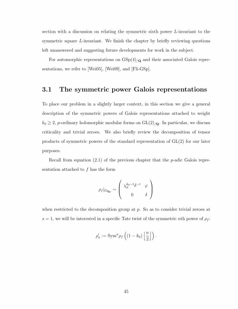
Recall from equation (2.1) of the previous chapter that the p-adic Galois repre-

sentation attached to f has the form

ρf |GQp∼

χk0−1p δ−1 ϕ

0 δ

when restricted to the decomposition group at p. So as to consider trivial zeroes at

s = 1, we will be interested in a specific Tate twist of the symmetric nth power of ρf :

ρ′n := Symnρf

((1− k0)

⌊n2

⌋).

45

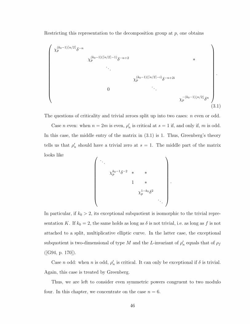
Restricting this representation to the decomposition group at p, one obtains

χ(k0−1)dn/2ep δ−n

χ(k0−1)(dn/2e−1)p δ−n+2 ∗

. . .

χ(k0−1)(dn/2e−i)p δ−n+2i

0. . .

χ−(k0−1)bn/2cp δn

.

(3.1)

The questions of criticality and trivial zeroes split up into two cases: n even or odd.

Case n even: when n = 2m is even, ρ′n is critical at s = 1 if, and only if, m is odd.

In this case, the middle entry of the matrix in (3.1) is 1. Thus, Greenberg’s theory

tells us that ρ′n should have a trivial zero at s = 1. The middle part of the matrix

looks like

. . .

χk0−1p δ−2 ∗ ∗

1 ∗

χ1−k0p δ2

. . .

.

In particular, if k0 > 2, its exceptional subquotient is isomorphic to the trivial repre-

sentation K. If k0 = 2, the same holds as long as δ is not trivial, i.e. as long as f is not

attached to a split, multiplicative elliptic curve. In the latter case, the exceptional

subquotient is two-dimensional of type M and the L-invariant of ρ′n equals that of ρf

([G94, p. 170]).

Case n odd: when n is odd, ρ′n is critical. It can only be exceptional if δ is trivial.

Again, this case is treated by Greenberg.

Thus, we are left to consider even symmetric powers congruent to two modulo

four. In this chapter, we concentrate on the case n = 6.

46

3.1.1 Just enough on finite-dimensional representations of

GL(2)

Recall that the irreducible finite-dimensional characteristic zero representations of

GL(2) are

SymaM ⊗ detb

for a ∈ Z≥0, b ∈ Z, where M denotes the standard representation. We will use the fol-

lowing decomposition of the tensor product of two symmetric power representations:

for a ≥ b ∈ Z≥0

SymaM ⊗ SymbM ∼=b⊕i=0

(Syma+b−2iM ⊗ deti

). (3.2)

Additionally, the following self-duality (up to a twist) will be useful:

(SymaM)∨ ∼= SymaM ⊗ det−a. (3.3)

3.2 The symmetric cube lifting to GSp(4)/Q

Let f be a p-ordinary, holomorphic, non-CM, cuspidal eigenform, new of level N

(prime to p), of even weight k0 ≥ 2, and trivial character. The added hypotheses on

the weight, the character, and non-CM are present so that we may use the symmetric

cube lifting to GSp(4)/Q of Ramakrishnan–Shahidi ([RS07, Theorem A′]). We briefly

review the statement of this theorem.

As in chapter 2, we write ρf for the p-adic Galois representation attached to f . Let

ρ3 := Sym3ρf and let π denote the cuspidal automorphic representation of GL(2,A)

defined by f . We have the following automorphy result for the symmetric cube of π.

47

Theorem 3.2.1 (Ramakrishnan–Shahidi, [RS07]). There exists a cuspidal automor-

phic representation Π of GSp(4,A) of trivial character, unramified away from N , such

that

a) Π∞ is in the holomorphic discrete series, with its L-parameter being the sym-

metric cube of that of π∞;

b) L(s,Π) = L(s, π, Sym3

).

Furthermore,

• ΠK 6= 0 for some compact open subgroup K of GSp(4,Af ) of level equal to the

conductor of ρ3;

• Π is of cohomological weight (a0, b0) = (2(k0 − 2), k0 − 2).3

3.3 The Hida deformation of ρ3

In this section and the following, we add a simplifying assumption:

(RAI) ρ3 is residually absolutely irreducible.

Without this assumption, one may still obtain a formula for the L-invariant (see

remarks 3.4.5a) and 3.4.8c) below). We will also assume k0 ≥ 4 and condition (Unr)

below to be able to apply the results of [TU99] without modification.

For the explicit matrices with which we will be dealing, we choose the Borel

subgroup, B4, of GSp(4) as in [RoSch07, Chapter 2] so that it consists of upper-

3Here, by cohomological weight, we mean (k1− 3, k2− 3) (as in [TU99]), where (k1, k2) gives thehighest weight of the lowest K∞-type of Π∞, as described in [Wei05] or [Wei09].

48

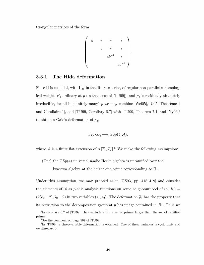
triangular matrices of the form

a ∗ ∗ ∗

b ∗ ∗

cb−1 ∗

ca−1

.

3.3.1 The Hida deformation

Since Π is cuspidal, with Π∞ in the discrete series, of regular non-parallel cohomolog-

ical weight, B4-ordinary at p (in the sense of [TU99]), and ρ3 is residually absolutely

irreducible, for all but finitely many4 p we may combine [Wei05], [U05, Theoreme 1

and Corollaire 1], and [TU99, Corollary 6.7] with [TU99, Theorem 7.1] and [Ny96]5

to obtain a Galois deformation of ρ3,

ρ3 : GQ −→ GSp(4,A),

where A is a finite flat extension of ΛJT1, T2K.6 We make the following assumption:

(Unr) the GSp(4) universal p-adic Hecke algebra is unramified over the

Iwasawa algebra at the height one prime corresponding to Π.

Under this assumption, we may proceed as in [GS93, pp. 418–419] and consider

the elements of A as p-adic analytic functions on some neighbourhood of (a0, b0) =

(2(k0− 2), k0− 2) in two variables (s1, s2). The deformation ρ3 has the property that

its restriction to the decomposition group at p has image contained in B4. Thus we

4In corollary 6.7 of [TU99], they exclude a finite set of primes larger than the set of ramifiedprimes.

5See the comment on page 567 of [TU99].6In [TU99], a three-variable deformation is obtained. One of these variables is cyclotomic and

we disregard it.

49

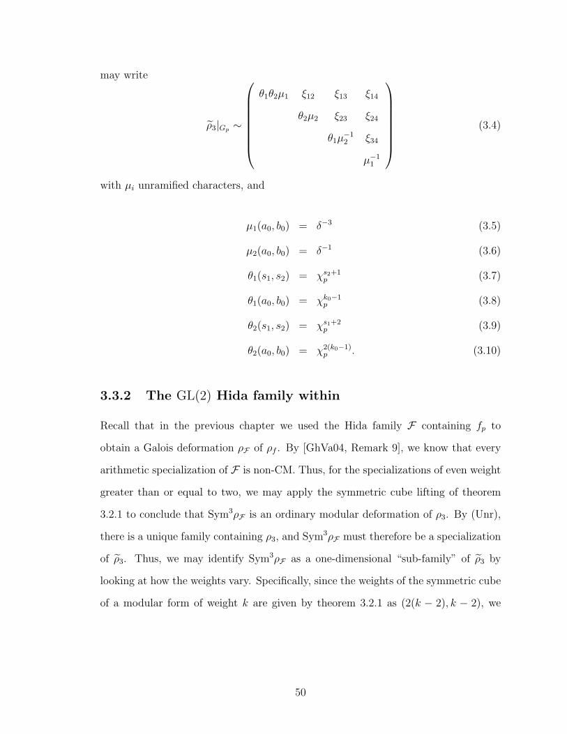
may write

ρ3|Gp ∼

θ1θ2µ1 ξ12 ξ13 ξ14

θ2µ2 ξ23 ξ24

θ1µ−12 ξ34

µ−11

(3.4)

with µi unramified characters, and

µ1(a0, b0) = δ−3 (3.5)

µ2(a0, b0) = δ−1 (3.6)

θ1(s1, s2) = χs2+1p (3.7)

θ1(a0, b0) = χk0−1p (3.8)

θ2(s1, s2) = χs1+2p (3.9)

θ2(a0, b0) = χ2(k0−1)p . (3.10)

3.3.2 The GL(2) Hida family within

Recall that in the previous chapter we used the Hida family F containing fp to

obtain a Galois deformation ρF of ρf . By [GhVa04, Remark 9], we know that every

arithmetic specialization of F is non-CM. Thus, for the specializations of even weight

greater than or equal to two, we may apply the symmetric cube lifting of theorem

3.2.1 to conclude that Sym3ρF is an ordinary modular deformation of ρ3. By (Unr),

there is a unique family containing ρ3, and Sym3ρF must therefore be a specialization

of ρ3. Thus, we may identify Sym3ρF as a one-dimensional “sub-family” of ρ3 by

looking at how the weights vary. Specifically, since the weights of the symmetric cube

of a modular form of weight k are given by theorem 3.2.1 as (2(k − 2), k − 2), we

50

conclude that Sym3ρF corresponds to the sub-family where

s1 = 2s2.

From identifying Sym3ρF with the specialization of ρ3 along this family, we obtain

the equations

µ1(2s, s) = µ−3(s+ 2)

µ2(2s, s) = µ−1(s+ 2).

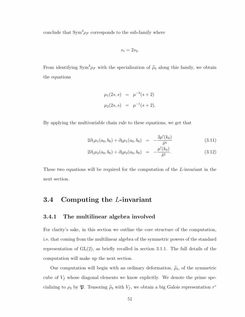
By applying the multivariable chain rule to these equations, we get that

2∂1µ1(a0, b0) + ∂2µ1(a0, b0) = −3µ′(k0)

δ4(3.11)

2∂1µ2(a0, b0) + ∂2µ2(a0, b0) = −µ′(k0)

δ2. (3.12)

These two equations will be required for the computation of the L-invariant in the

next section.

3.4 Computing the L-invariant

3.4.1 The multilinear algebra involved

For clarity’s sake, in this section we outline the core structure of the computation,

i.e. that coming from the multilinear algebra of the symmetric powers of the standard

representation of GL(2), as briefly recalled in section 3.1.1. The full details of the

computation will make up the next section.

Our computation will begin with an ordinary deformation, ρ3, of the symmetric

cube of Vf whose diagonal elements we know explicitly. We denote the prime spe-

cializing to ρ3 by P. Tensoring ρ3 with Vf , we obtain a big Galois representation r◦

51

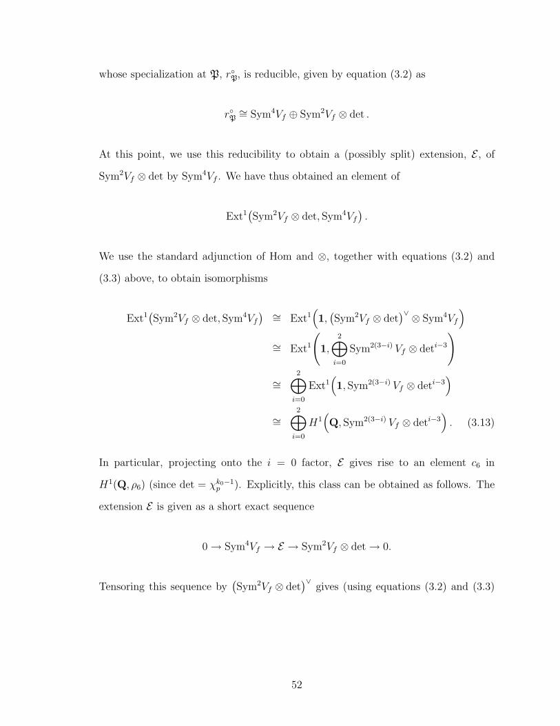
whose specialization at P, r◦P, is reducible, given by equation (3.2) as

r◦P∼= Sym4Vf ⊕ Sym2Vf ⊗ det .

At this point, we use this reducibility to obtain a (possibly split) extension, E , of

Sym2Vf ⊗ det by Sym4Vf . We have thus obtained an element of

Ext1(Sym2Vf ⊗ det, Sym4Vf

).

We use the standard adjunction of Hom and ⊗, together with equations (3.2) and

(3.3) above, to obtain isomorphisms

Ext1(Sym2Vf ⊗ det, Sym4Vf

) ∼= Ext1(1,(Sym2Vf ⊗ det

)∨ ⊗ Sym4Vf

)∼= Ext1

(1,

2⊕i=0

Sym2(3−i) Vf ⊗ deti−3

)

∼=2⊕i=0

Ext1(1, Sym2(3−i) Vf ⊗ deti−3

)∼=

2⊕i=0

H1(Q, Sym2(3−i) Vf ⊗ deti−3

). (3.13)

In particular, projecting onto the i = 0 factor, E gives rise to an element c6 in

H1(Q, ρ6) (since det = χk0−1p ). Explicitly, this class can be obtained as follows. The

extension E is given as a short exact sequence

0→ Sym4Vf → E → Sym2Vf ⊗ det→ 0.

Tensoring this sequence by(Sym2Vf ⊗ det

)∨gives (using equations (3.2) and (3.3)

52

once again)

0→2⊕i=0

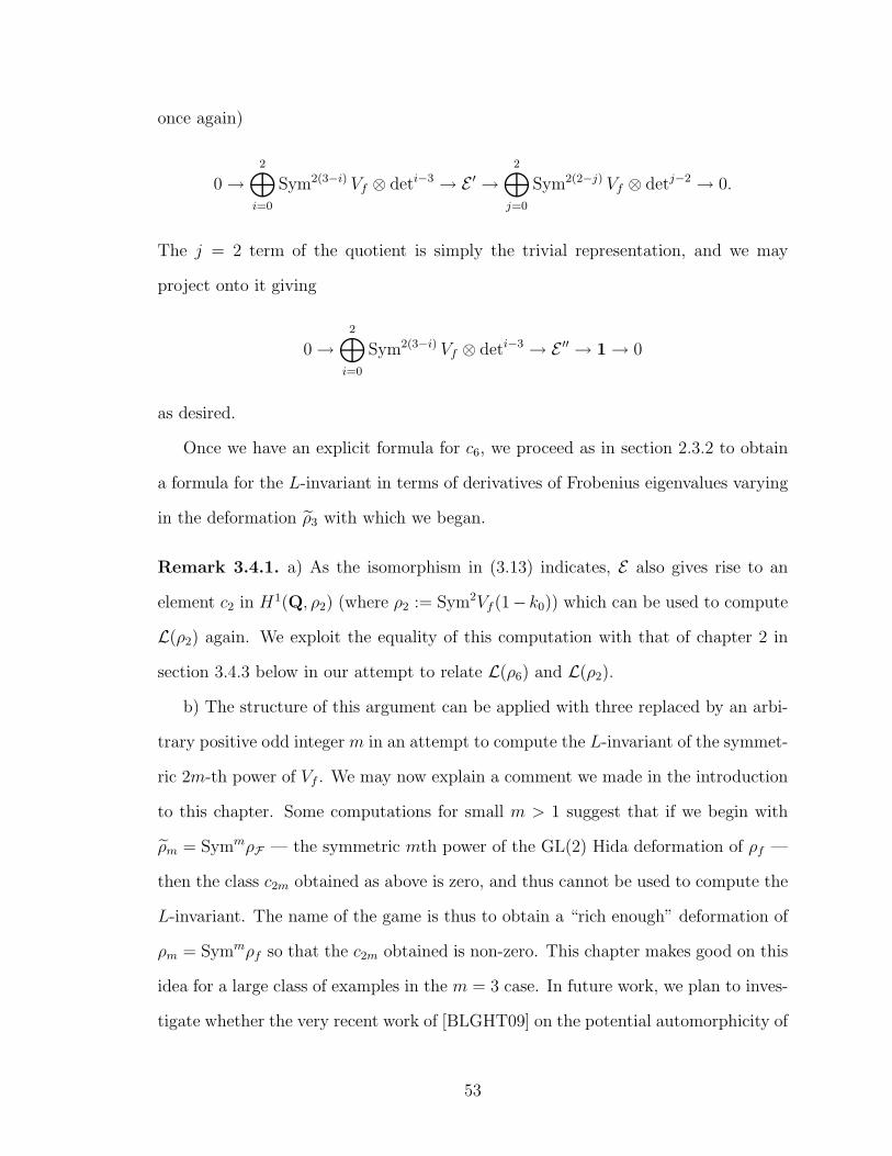
Sym2(3−i) Vf ⊗ deti−3 → E ′ →2⊕j=0

Sym2(2−j) Vf ⊗ detj−2 → 0.

The j = 2 term of the quotient is simply the trivial representation, and we may

project onto it giving

0→2⊕i=0

Sym2(3−i) Vf ⊗ deti−3 → E ′′ → 1→ 0

as desired.

Once we have an explicit formula for c6, we proceed as in section 2.3.2 to obtain

a formula for the L-invariant in terms of derivatives of Frobenius eigenvalues varying

in the deformation ρ3 with which we began.

Remark 3.4.1. a) As the isomorphism in (3.13) indicates, E also gives rise to an

element c2 in H1(Q, ρ2) (where ρ2 := Sym2Vf (1− k0)) which can be used to compute

L(ρ2) again. We exploit the equality of this computation with that of chapter 2 in

section 3.4.3 below in our attempt to relate L(ρ6) and L(ρ2).

b) The structure of this argument can be applied with three replaced by an arbi-

trary positive odd integer m in an attempt to compute the L-invariant of the symmet-

ric 2m-th power of Vf . We may now explain a comment we made in the introduction

to this chapter. Some computations for small m > 1 suggest that if we begin with

ρm = SymmρF — the symmetric mth power of the GL(2) Hida deformation of ρf —

then the class c2m obtained as above is zero, and thus cannot be used to compute the

L-invariant. The name of the game is thus to obtain a “rich enough” deformation of

ρm = Symmρf so that the c2m obtained is non-zero. This chapter makes good on this

idea for a large class of examples in the m = 3 case. In future work, we plan to inves-

tigate whether the very recent work of [BLGHT09] on the potential automorphicity of

53

the symmetric powers of higher weight modular forms can be paired succesfully with

Hida’s ordinary families on unitary groups ([Hi02]) to yield L-invariants of higher

symmetric powers.

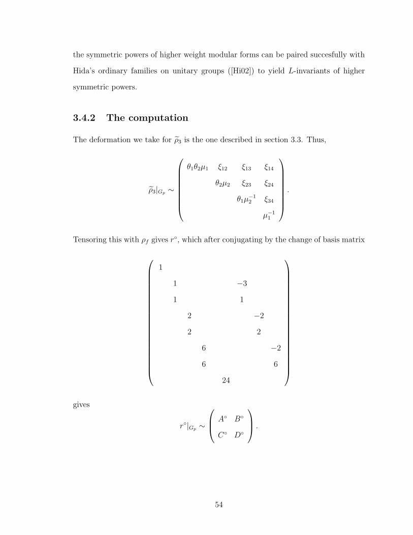
3.4.2 The computation

The deformation we take for ρ3 is the one described in section 3.3. Thus,

ρ3|Gp ∼

θ1θ2µ1 ξ12 ξ13 ξ14

θ2µ2 ξ23 ξ24

θ1µ−12 ξ34

µ−11

.

Tensoring this with ρf gives r◦, which after conjugating by the change of basis matrix

1

1 −3

1 1

2 −2

2 2

6 −2

6 6

24

gives

r◦|Gp ∼

A◦ B◦

C◦ D◦

.

54

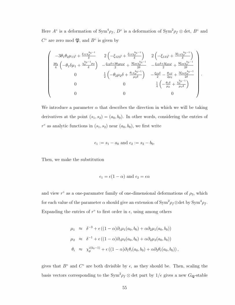
Here A◦ is a deformation of Sym4ρf , D◦ is a deformation of Sym2ρf ⊗ det, B◦ and

C◦ are zero mod P, and B◦ is given by

−3θ1θ2µ1ϕ+ξ12χ

k0−1p

δ2(−ξ12ϕ+

ξ13χk0−1p

δ

)2(−ξ13ϕ+

3ξ14χk0−1p

δ

)3θ24

(−θ1δµ1 +

χk0−1p µ2

δ

)− ξ12δ+3θ2µ2ϕ

2+

3ξ23χk0−1p

2δ− ξ13δ+3ξ23ϕ

2+

9ξ24χk0−1p

2δ

0 12

(−θ2µ2δ +

θ1χk0−1p

µ2δ

)− ξ23δ

2− θ1ϕ

2µ2+

3ξ34χk0−1p

2δ

0 0 14

(− θ1δ

µ2+

χk0−1p

µ1δ

)0 0 0

.

We introduce a parameter α that describes the direction in which we will be taking

derivatives at the point (s1, s2) = (a0, b0). In other words, considering the entries of

r◦ as analytic functions in (s1, s2) near (a0, b0), we first write

ε1 := s1 − a0 and ε2 := s2 − b0.

Then, we make the substitution

ε1 = ε(1− α) and ε2 = εα

and view r◦ as a one-paramater family of one-dimensional deformations of ρ3, which

for each value of the parameter α should give an extension of Sym2ρf⊗det by Sym4ρf .

Expanding the entries of r◦ to first order in ε, using among others

µ1 ≈ δ−3 + ε ((1− α)∂1µ1(a0, b0) + α∂2µ1(a0, b0))

µ2 ≈ δ−1 + ε ((1− α)∂1µ2(a0, b0) + α∂2µ2(a0, b0))

θi ≈ χi(k0−1)p + ε ((1− α)∂1θi(a0, b0) + α∂2θi(a0, b0)) ,

gives that B◦ and C◦ are both divisible by ε, as they should be. Then, scaling the

basis vectors corresponding to the Sym2ρf ⊗ det part by 1/ε gives a new GQ-stable

55

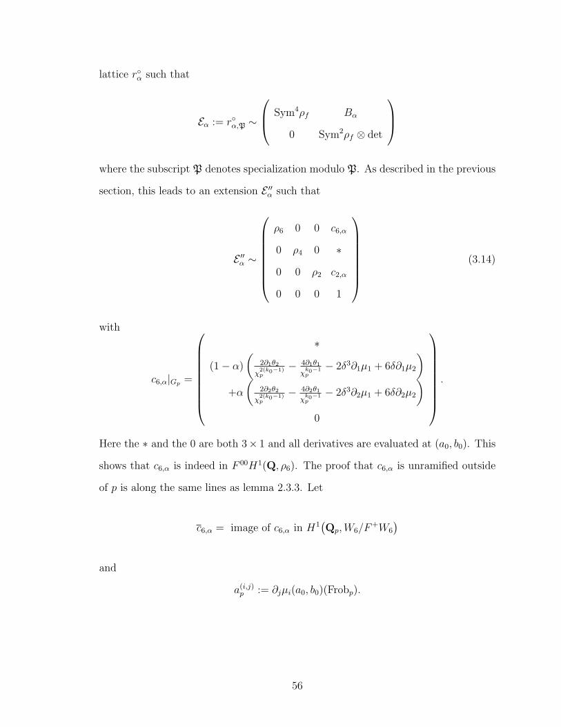
lattice r◦α such that

Eα := r◦α,P ∼

Sym4ρf Bα

0 Sym2ρf ⊗ det

where the subscript P denotes specialization modulo P. As described in the previous

section, this leads to an extension E ′′α such that

E ′′α ∼

ρ6 0 0 c6,α

0 ρ4 0 ∗

0 0 ρ2 c2,α

0 0 0 1

(3.14)

with

c6,α|Gp =

∗

(1− α)

(2∂1θ2

χ2(k0−1)p

− 4∂1θ1

χk0−1p

− 2δ3∂1µ1 + 6δ∂1µ2

)+α

(2∂2θ2

χ2(k0−1)p

− 4∂2θ1

χk0−1p

− 2δ3∂2µ1 + 6δ∂2µ2

)0

.

Here the ∗ and the 0 are both 3× 1 and all derivatives are evaluated at (a0, b0). This

shows that c6,α is indeed in F 00H1(Q, ρ6). The proof that c6,α is unramified outside

of p is along the same lines as lemma 2.3.3. Let

c6,α = image of c6,α in H1(Qp,W6/F

+W6

)and

a(i,j)p := ∂jµi(a0, b0)(Frobp).

56

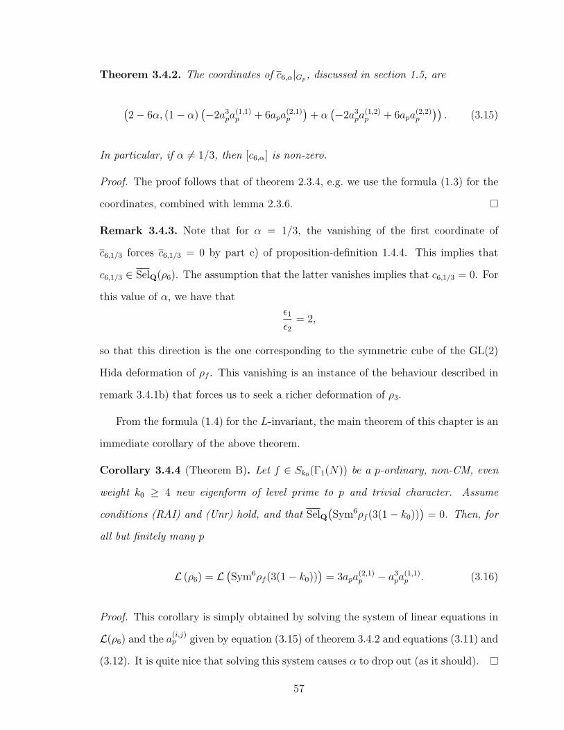
Theorem 3.4.2. The coordinates of c6,α|Gp, discussed in section 1.5, are

(2− 6α, (1− α)

(−2a3

pa(1,1)p + 6apa

(2,1)p

)+ α

(−2a3

pa(1,2)p + 6apa

(2,2)p

)). (3.15)

In particular, if α 6= 1/3, then [c6,α] is non-zero.

Proof. The proof follows that of theorem 2.3.4, e.g. we use the formula (1.3) for the

coordinates, combined with lemma 2.3.6.

Remark 3.4.3. Note that for α = 1/3, the vanishing of the first coordinate of

c6,1/3 forces c6,1/3 = 0 by part c) of proposition-definition 1.4.4. This implies that

c6,1/3 ∈ SelQ(ρ6). The assumption that the latter vanishes implies that c6,1/3 = 0. For

this value of α, we have that

ε1ε2

= 2,

so that this direction is the one corresponding to the symmetric cube of the GL(2)

Hida deformation of ρf . This vanishing is an instance of the behaviour described in

remark 3.4.1b) that forces us to seek a richer deformation of ρ3.

From the formula (1.4) for the L-invariant, the main theorem of this chapter is an

immediate corollary of the above theorem.

Corollary 3.4.4 (Theorem B). Let f ∈ Sk0(Γ1(N)) be a p-ordinary, non-CM, even

weight k0 ≥ 4 new eigenform of level prime to p and trivial character. Assume

conditions (RAI) and (Unr) hold, and that SelQ(Sym6ρf (3(1− k0))

)= 0. Then, for

all but finitely many p

L (ρ6) = L(Sym6ρf (3(1− k0))

)= 3apa

(2,1)p − a3

pa(1,1)p . (3.16)

Proof. This corollary is simply obtained by solving the system of linear equations in

L(ρ6) and the a(i,j)p given by equation (3.15) of theorem 3.4.2 and equations (3.11) and

(3.12). It is quite nice that solving this system causes α to drop out (as it should).

57

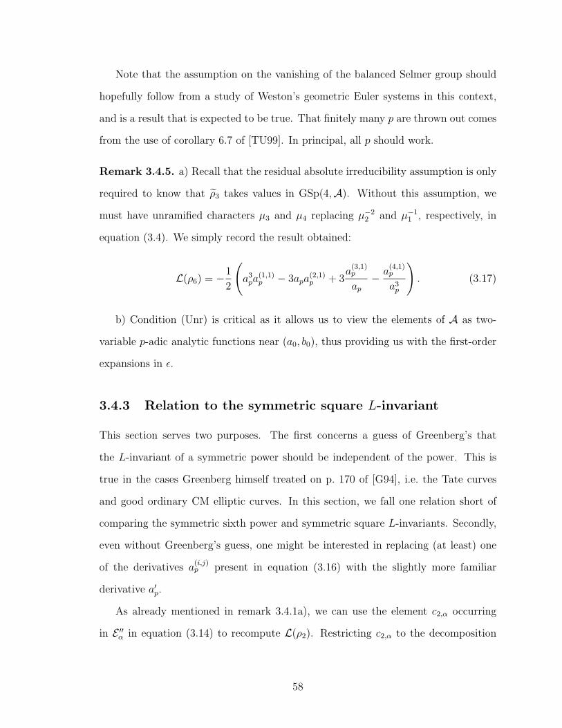
Note that the assumption on the vanishing of the balanced Selmer group should

hopefully follow from a study of Weston’s geometric Euler systems in this context,

and is a result that is expected to be true. That finitely many p are thrown out comes

from the use of corollary 6.7 of [TU99]. In principal, all p should work.

Remark 3.4.5. a) Recall that the residual absolute irreducibility assumption is only

required to know that ρ3 takes values in GSp(4,A). Without this assumption, we

must have unramified characters µ3 and µ4 replacing µ−22 and µ−1

1 , respectively, in

equation (3.4). We simply record the result obtained:

L(ρ6) = −1

2

(a3pa

(1,1)p − 3apa

(2,1)p + 3

a(3,1)p

ap− a

(4,1)p

a3p

). (3.17)

b) Condition (Unr) is critical as it allows us to view the elements of A as two-

variable p-adic analytic functions near (a0, b0), thus providing us with the first-order

expansions in ε.

3.4.3 Relation to the symmetric square L-invariant

This section serves two purposes. The first concerns a guess of Greenberg’s that

the L-invariant of a symmetric power should be independent of the power. This is

true in the cases Greenberg himself treated on p. 170 of [G94], i.e. the Tate curves

and good ordinary CM elliptic curves. In this section, we fall one relation short of

comparing the symmetric sixth power and symmetric square L-invariants. Secondly,

even without Greenberg’s guess, one might be interested in replacing (at least) one

of the derivatives a(i,j)p present in equation (3.16) with the slightly more familiar

derivative a′p.

As already mentioned in remark 3.4.1a), we can use the element c2,α occurring

in E ′′α in equation (3.14) to recompute L(ρ2). Restricting c2,α to the decomposition

58

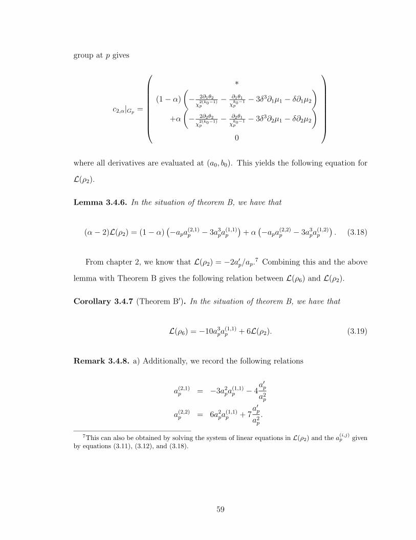
group at p gives

c2,α|Gp =

∗

(1− α)

(− 2∂1θ2

χ2(k0−1)p

− ∂1θ1

χk0−1p

− 3δ3∂1µ1 − δ∂1µ2

)+α

(− 2∂2θ2

χ2(k0−1)p

− ∂2θ1

χk0−1p

− 3δ3∂2µ1 − δ∂2µ2

)0

where all derivatives are evaluated at (a0, b0). This yields the following equation for

L(ρ2).

Lemma 3.4.6. In the situation of theorem B, we have that

(α− 2)L(ρ2) = (1− α)(−apa(2,1)

p − 3a3pa

(1,1)p

)+ α

(−apa(2,2)

p − 3a3pa

(1,2)p

). (3.18)

From chapter 2, we know that L(ρ2) = −2a′p/ap.7 Combining this and the above

lemma with Theorem B gives the following relation between L(ρ6) and L(ρ2).

Corollary 3.4.7 (Theorem B′). In the situation of theorem B, we have that

L(ρ6) = −10a3pa

(1,1)p + 6L(ρ2). (3.19)

Remark 3.4.8. a) Additionally, we record the following relations

a(2,1)p = −3a2

pa(1,1)p − 4

a′pa2p

a(2,2)p = 6a2

pa(1,1)p + 7

a′pa2p

.

7This can also be obtained by solving the system of linear equations in L(ρ2) and the a(i,j)p given

by equations (3.11), (3.12), and (3.18).

59

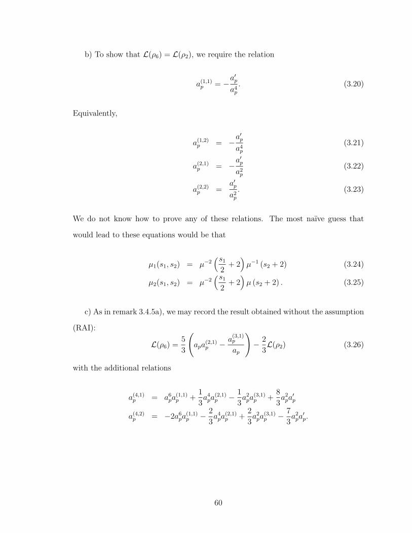
b) To show that L(ρ6) = L(ρ2), we require the relation

a(1,1)p = −

a′pa4p

. (3.20)

Equivalently,

a(1,2)p = −

a′pa4p

(3.21)

a(2,1)p = −

a′pa2p

(3.22)

a(2,2)p =

a′pa2p

. (3.23)

We do not know how to prove any of these relations. The most naıve guess that

would lead to these equations would be that

µ1(s1, s2) = µ−2(s1

2+ 2)µ−1 (s2 + 2) (3.24)

µ2(s1, s2) = µ−2(s1

2+ 2)µ (s2 + 2) . (3.25)

c) As in remark 3.4.5a), we may record the result obtained without the assumption

(RAI):

L(ρ6) =5

3

(apa

(2,1)p − a

(3,1)p

ap

)− 2

3L(ρ2) (3.26)

with the additional relations

a(4,1)p = a6

pa(1,1)p +

1

3a4pa

(2,1)p − 1

3a2pa

(3,1)p +

8

3a2pa′p

a(4,2)p = −2a6

pa(1,1)p − 2

3a4pa

(2,1)p +

2

3a2pa

(3,1)p − 7

3a2pa′p.

60

3.5 Concluding remarks

Many of the remarks made at the end of the previous chapter can be made here as

well. Indeed, we do not deal with the question of globalness, the non-vanishing, nor

the relation to the p-adic L-function. The only work we are aware of on any of these

questions is again the work of Greenberg and Hida relating the L-invariant to the

arithmetic p-adic L-function.

In Hida’s work (e.g. [Hi07]), he uses Ad0ρm to study ρ2m. Though we have not

verified the computations, we suspect that, as in the previous chapter we could use

Ad0ρf , in this chapter we could use Ad0ρ3.

The results of this chapter suggest that higher symmetric powers can be addressed

via new cases of functoriality. A particular instance we have in mind is the very recent

work of [BLGHT09] on the potential automorphicity of symmetric powers of higher

weight modular forms as automorphic forms on unitary groups. We would hope that,

together with Hida theory on unitary groups ([Hi02]), this would yield further results

in this subject. The work of Harris–Li–Skinner on several variable p-adic L-functions

attached to Hida families on unitary groups in [HLS06] additionally provides a basis

for attempting to relate Greenberg’s L-invariant of symmetric powers of modular

forms to analytic p-adic L-functions. All factors indicate that there is much work

ahead.

61

Bibliography

Books and Proceedings

[ANT-Hyd] Rajat Tandon (ed.), Algebra and number theory, Hindustan Book

Agency, 2005.

[ANT-Iwa] John Coates, Ralph Greenberg, Barry Mazur, and Ichiro Satake (eds.),

Algebraic number theory, Advanced Studies in Pure Mathematics,

vol. 17, Academic Press, 1989, Papers in honor of Kenkichi Iwasawa

on the occasion of his 70th birthday on September 11, 1987.

[Bures] Jean-Marc Fontaine (ed.), Periodes p-adiques, Asterisque, vol. 223, SMF,

1994, Seminaire de Bures, 1988.

[Corv] Armand Borel and William Casselman (eds.), Automorphic forms, rep-

resentations, and L-functions, Proceedings of the Symposium in Pure

Mathematics, vol. 33, AMS, 1979, in two parts.

[FAII] Henri Carayol, Michael Harris, Jacques Tilouine, and Marie-France

Vigneras (eds.), Formes automorphes (II): Le cas du groupe GSp(4),

Asterisque, vol. 302, SMF, 2005.

[Fli-GSp] Yuval Z. Flicker, Automorphic forms and Shimura varieties of PGSp(2),

World Scientific Publishing, 2005.

62

[GFest] Pierre Cartier, Luc Illusie, Nicholas M. Katz, Gerard Laumon, Yuri

Manin, and Ken Ribet (eds.), The Grothendieck Festschrift. Vol. I,

Progress in Mathematics, vol. 86, Birkhauser, 1990.

[Hi-HMI] Haruzo Hida, Hilbert modular forms and Iwasawa theory, Oxford Math-

ematical Monographs, Oxford University Press, 2006.

[M:FP] Vladimir I. Arnold, Michael Atiyah, and Barry Mazur (eds.), Mathemat-

ics: Frontiers and perspectives, AMS, 2000.

[pMBSD] Barry Mazur and Glenn Stevens (eds.), p-adic monodromy and the Birch

and Swinnerton-Dyer conjecture, Contemporary Mathematics, vol. 165,

AMS, 1994, Papers from the workshop held at Boston University, August

12–16, 1991.

[PR00] Bernadette Perrin-Riou, p-adic L-functions and p-adic representations,

SMF/AMS Texts and Monographs, vol. 3, AMS, 2000, translated from

the 1995 french original.

[RoSch07] Brooks Roberts and Ralf Schmidt, Local newforms for GSp(4), Lecture

Notes in Mathematics, vol. 1918, Springer-Verlag, 2007.

[Wei09] Rainer Weissauer, Endoscopy for GSp(4) and the cohomology of Siegel

modular threefolds, Lecture Notes in Mathematics, vol. 1968, Springer-

Verlag, 2009.

Articles

[Be09] Denis Benois, A generalization of Greenberg’s L-invariant, 2009,

preprint, arXiv:0906.2857v1 [math.NT].

[BK90] Spencer Bloch and Kazuya Kato, L-functions and Tamagawa numbers

of motives, in [GFest], 1990, pp. 333–400.

63

[BLGHT09] Thomas Barnet-Lamb, David Geraghty, Michael Harris, and Richard

Taylor, A family of Calabi–Yau varieties and potential automorphy. II,

2009, preprint from Richard Taylor’s website.

[Ci08] Craig Citro, L-invariants of adjoint square Galois representations com-

ing from modular forms, Int. Math. Res. Not. (2008), no. 14, Art. ID

rnn048.

[Co89] John Coates, On p-adic L-functions attached to motives over Q. II, Bol.

Soc. Brasil. Mat. (N.S.) 20 (1989), no. 1, 101–112.

[CoPR89] John Coates and Bernadette Perrin-Riou, On p-adic L-functions at-

tached to motives over Q, in [ANT-Iwa], 1989, pp. 23–54.

[Cz05] Pierre Colmez, Zeros supplementaires de fonctions L p-adiques de formes

modulaires, in [ANT-Hyd], 2005, pp. 193–210.

[D71] Pierre Deligne, Formes modulaires et representations `-adiques,

Seminaire Bourbaki 1968/69 (1971), no. 355, 139–172.

[D79] Pierre Deligne, Valeurs de fonctions L et periodes d’integrales, in [Corv],

part 2, 1979, pp. 313–346.

[Em06] Matthew Emerton, A local-global compatibility conjecture in the p-adic

Langlands programme for GL2/Q, Pure Appl. Math. Q. 2 (2006), no. 2,

279–393.

[Fl90] Matthias Flach, A generalisation of the Cassels–Tate pairing, J. Reine

Angew. Math. 412 (1990), 113–127.

[G89] Ralph Greenberg, Iwasawa theory for p-adic representations, in

[ANT-Iwa], 1989, pp. 97–137.

64

[G94] Ralph Greenberg, Trivial zeroes of p-adic L-functions, in [pMBSD],

1994, pp. 149–174.

[GhVa04] Eknath Ghate and Vinayak Vatsal, On the local behaviour of ordinary

Λ-adic representations, Ann. Inst. Fourier (Grenoble) 54 (2004), no. 7,

2143–2162.

[GS93] Ralph Greenberg and Glenn Stevens, p-adic L-functions and p-adic pe-

riods of modular forms, Invent. Math. 111 (1993), no. 2, 407–447.

[Hi86] Haruzo Hida, Galois representations into GL2(ZpJxK) attached to ordi-

nary cusp forms, Invent. Math. 85 (1986), no. 3, 545–613.

[Hi00] Haruzo Hida, Adjoint Selmer groups as Iwasawa modules, Israel J. Math.

200 (2000), 361–427.

[Hi02] Haruzo Hida, Control theorems of coherent sheaves on Shimura varieties

of PEL type, J. Inst. Math. Jussieu 1 (2002), no. 1, 1–76.

[Hi04] Haruzo Hida, Greenberg’s L-invariants of adjoint square Galois repre-

sentations, Int. Math. Res. Not. (2004), no. 59, 3177–3189.

[Hi07] Haruzo Hida, On a generalization of the conjecture of Mazur–Tate–

Teitelbaum, Int. Math. Res. Not. (2007), no. 23, Art. ID rnm102.

[HLS06] Michael Harris, Jian-Shu Li, and Christopher Skinner, p-adic L-

functions for unitary Shimura varieties. I. Construction of the Eisenstein

measure, Doc. Math. Extra Vol. (2006), 393–464.

[Ki04] Mark Kisin, Geometric deformations of modular Galois representations,

Invent. Math. 157 (2004), no. 2, 275–328.

65

[MTT86] Barry Mazur, John Tate, and Jeremy Teitelbaum, On p-adic analogues of

the conjectures of Birch and Swinnerton-Dyer, Invent. Math. 84 (1986),

no. 1, 1–48.

[Mz72] Barry Mazur, Rational points of abelian varieties with values in towers

of number fields, Invent. Math. 18 (1972), 183–266.

[Mz00] Barry Mazur, The theme of p-adic variation, in [M:FP], 2000, pp. 433–

459.

[MzW86] Barry Mazur and Andrew Wiles, On p-adic analytic families of Galois

representations, Compositio Math. 59 (1986), no. 2, 231–264.

[Ny96] Louise Nyssen, Pseudo-representations, Math. Ann. 306 (1996), no. 2,

257–283.

[Po09] Jonathan Pottharst, Generalizations of Greenberg’s “ordinary” condi-

tion, I, 2009, preprint from the author’s website.

[PR94] Bernadette Perrin-Riou, Representations p-adiques ordinaires, in

[Bures], 1994, pp. 185–220.

[Ri76] Ken Ribet, A modular construction of unramified p-extensions of Q(µp),

Invent. Math. 34 (1976), no. 3, 151–162.

[RS07] Dinakar Ramakrishnan and Freydoon Shahidi, Siegel modular forms of

genus 2 attached to elliptic curves, Math. Res. Let. 14 (2007), no. 2,

315–332.

[TU99] Jacques Tilouine and Eric Urban, Several-variable p-adic families

of Siegel–Hilbert cusp eigensystems and their Galois representations,

Ann. Sci. Ecole Norm. Sup. 32 (1999), no. 4, 499–574.

66

[U05] Eric Urban, Sur les representations p-adiques associees aux

representations cuspidales de GSp4/Q, in [FAII], 2005, pp. 151–176.

[W88] Andrew Wiles, On ordinary λ-adic representations associated to modular

forms, Invent. Math. 94 (1988), no. 3, 529–573.

[W95] Andrew Wiles, Modular elliptic curves and Fermat’s last theorem,

Ann. of Math. (2) 141 (1995), no. 3, 443–551.

[Wei05] Rainer Weissauer, Four dimensional Galois representations, in [FAII],

2005, pp. 67–150.

[Wes04] Tom Weston, Geometric Euler systems for locally isotropic motives,

Compos. Math. 140 (2004), no. 2, 317–332.

67