Time in GIS: Issues in spatio-temporal modelling L. Heres (editor)

NCG Nederlandse Commissie voor Geodesie Netherlands Geodetic Commission Delft, May 2000

Colophon Time in GIS: Issues in spatio-temporal modelling L. Heres (editor) Publications on Geodesy 47 ISBN 90 6132 269 3 ISSN 0165 1706 Publications on Geodesy is the continuation of Publications on Geodesy New Series Published by: NCG Nederlandse Commissie voor Geodesie Netherlands Geodetic Com-mission, Delft, The Netherlands Printed by: Meinema Drukkerij, Delft, The Netherlands NCG Nederlandse Commissie voor Geodesie P.O. Box 5030, 2600 GA Delft, The Netherlands Tel.: +31 (0)15 278 28 19 Fax: +31 (0)15 278 17 75 E-mail: ncg@geo.tudelft.nl WWW: www.ncg.knaw.nl The NCG Nederlandse Commissie voor Geodesie Netherlands Geodetic Commission is an institute of the Royal Netherlands Academy of Arts and Sciences (KNAW).

ii

Contents Luc Heres Time in GIS: Issues in spatio-temporal modelling 1 Donna J. Peuquet Space-time representation: An overview 3 Monica Wachowicz The role of geographic visualisation and knowledge discovery in spatio-temporal data modelling 13 Menno-Jan Kraak Visualisation of the time dimension 27 Peter van Oosterom Time in cadastral maps 36 Luc Heres Hodochronologics: History and time in the National Road Database 46 Ipo Ritsema Time in relation to geoscientific data 57

iii

Time in GIS: Issues in spatio-temporal modelling Luc Heres Most Geographic Information Systems started as a substitute for loose paper maps. These paper maps did not have a built-in time dimension and could only represent history indirectly as a sequence of physically separate images. This was in fact imitated by these first genera-tion systems. The time dimension could only be represented by means of separate files. A minority of Geographic Information Systems however, started their life as a substitute for ordered lists and tables with a link to paper maps. In these lists, the inclusion of a time com-ponent in the form of a data field was quite usual. This method too was copied by the systems that replaced these paper tables. The current trend in the development of Geographic Information Systems is towards the inte-gration of the classical map-oriented concepts with the table-oriented concepts. This often leads to the explicit embedding of the time component in the GIS environment. The Subcommision Geo-Information Models of the Netherlands Geodetic Commission has organized a workshop to discuss the theory and practice of time and history in GIS on 18 May 2000. This publication contains 6 articles prepared for the workshop. The first paper, written by Donna Peuquet, gives a bird’s-eye view of the current state of the art in spatio-temporal database technology and methodology. She is a well-known expert in the field of spatio-temporal information systems and the author of many articles in this field. The second article is written by Monica Wachowicz. She describes what you can do with a GIS once it contains a historical dimension and how you can detect changes in geographic phenomena. Furthermore, her article suggests how geographic visualisation and knowledge discovery techniques can be integrated in a spatio-temporal database. How to record the time dimension in a database is one thing, how to show this dimension to users is another one. In his contribution, Menno-Jan Kraak first tells about the techniques, which were used in the age of paper maps and the limitations these methods had. He goes on to explain what kind of cartographic techniques have been developed since the mass introduc-tion of the computer. Finally he describes the powerful animation methods which currently exist and can be used on CD-ROM and Internet applications. Peter van Oosterom describes how the time dimension is represented in the information sys-tems of the Cadastre and how this is used to publish updates. The Cadastre has a very long tradition in incorporating the time component, which has always been an inherent component of the cadastral registration. In former times this was translated in very precise procedures about how to update the paper maps and registers. Today it is translated in spatio-temporal database design.

1

The article of Luc Heres tells about the time component in the National Road Database, origi-nally designed for traffic accident registration. This is one of the systems with “table” roots and with quite a long tradition in handling the time dimension. He elucidates first the core objects in the conceptual model and how time is added. Next, how this model is translated in a logical design and finally how this is technically implemented. Geologists and geophysicians also have a respectable tradition in handling the time dimen-sion in the data they collect. This is illustrated in the last paper, which is written by Ipo Rit-sema. He outlines how time is handled in geological and geophysical databases maintained by TNO. By means of some practical cases he illustrates which problems can be encountered and how these can be solved.

2

Space-time representation: An overview Donna J. Peuquet Department of Geography and The GeoVista Center The Pennsylvania State University University Park, Pennsylvania, U.S.A. +814 863 0390 / +814 863 7943 (fax) peuquet@geog.psu.edu Introduction Geographic Information Systems (GIS) have become an essential tool for a wide variety of analy-sis contexts that effect our daily lives. These have now extended from the initial application areas of natural resource management and urban planning to include analysis of the global economy and climate change, as well as detection of patterns of disease. Such phenomena involve complex natural and human systems that are also often intertwined. Change through time, as well as over space, is an integral component of any geographic process. The analysis of temporal pattern - cycles and rhythms - is essential to the understanding of those processes and for the subsequent ability to predict and plan. The temporal dimension was nevertheless ignored in GIS until rela-tively recently. The reason for this is clear in retrospect in that current GIS techniques were derived using the traditional cartographic paradigm; the presentation of geographic space as a static snapshot. Cer-tainly, this view of the world had in large part been necessitated by the static nature of the carto-graphic media available before computers. Much research is now taking place in both the carto-graphic and GIS realms toward representation of space-time dynamics within a computing con-text. The computer as a new cartographic medium, with the ability to interact with a 2-d or 3-d dynamic map as an analytical tool has changed focus from cartographic presentation, as a mes-sage to be communicated in an end product, to cartographic representation, as portrayal of in-formation in a manner very closely allied with database models as an aid for solving problems. The real potential power of GIS is also now in reach within the foreseeable future. Because of the spatial data handling and analysis potential of GIS, their use is critical as an enabling technology as an exploratory tool for uncovering patterns and relationships. As yet, however, there are no means of truly exploring these data to uncover associations among people, places, and times in a way that truly represents a conceptual advancement over a sequence of paper maps. Although complex spatial interrelationships at a given point in time can be calculated using a GIS, calculat-ing temporal relationships between factors that occur in space can also be performed by essen-tially “tricking” the software. For example, how factors at a set of locations change over time can be determined by comparing a sequence of temporal overlays. With this technique, the standard overlay facility is used to compare layers representing the spatial distribution of a single variable at different times instead of different variables for a single time.

3

4

Using what are intended as spatial tools for temporal analysis is a very awkward process, and with intrinsic limitations. Langran’s groundbreaking work over ten years ago (1988; 1992) criti-cized GIS for its inability to explicitly represent change over time in the database, handle the simplest of temporal queries (e.g., queries involving “before” or “after relationships), or to even maintain multiple versions of a database as changes are made over time. Much has been written since on the subject of Temporal GIS. Some have proposed data models for space-time represen-tation (Hazelton, Leahy et al. 1990; Worboys 1994; Peuquet and Duan 1995), but construction of a fully functional Temporal GIS is still problematic. Initial attempts to simply extend currently used representational techniques to include time as either time slices or as incremental points, lines and areas have proven to either be inadequate for the task or unduly complex (Peuquet 1994). The basic problem is that most researchers have taken a short-term, implementational view. The effective representation of time in a database or on a computer display, and the appropriate analysis of space-time data, requires a better under-standing of the nature of time and the various ways available to conceptualize it. Fortunately, there is a vast literature already extant on this topic, and in a range of fields from philosophy and physics to geography. In this paper I will give a very brief review of the historic evolution of how space and time are conceptually represented in order to draw out the commonalities and the dif-ferences between them. I will then give a brief discussion of analysis within modern science of space-time dynamics for geographic-scale processes and the implications for moving forward in a computing context. What are "space" and "time"? Space and time are among the most fundamental of notions. They provide a basis for ordering all modes of thought and belief. We are constantly reminded of the importance of space and time in modern everyday life when we use such expressions in ordinary language as 'Everything has its place'. Here and there, then and now are references to a conceptual framework of knowledge about the world. In short, things occur or exist in relation to space and time. Although basic and often taken for granted in everyday life, the nature of both space and time is a complex issue. The dictionary definitions of the terms "space" and “time” perhaps provide more confusion than clari-fication. Webster's New Twentieth Century English Dictionary, second edition, defines "space" as: (1.) distance extending without limit in all directions; that which is thought of as a boundless,

continuous expanse extending in all directions or in three directions, within which all ma-terial things are contained

(2.) distance, interval, or area between or within things; extent; room; as 'leave a wide space between rows'

(3.) (enough) area or room for some purpose..." among a total of twelve separately enumerated definitions. For "time" the situation is even worse. In the same dictionary, "time" is variously defined as:

5

( 1.) the period between two events or during which something exists, happens, or acts: meas-ured or measurable interval

( 2.) a period of history, characterized by a given social structure, set of customs, etc.; as, me-dieval times

: (13.) a precise instant, second, minute, hour, day, week, month, or year, determined by clock or

calendar; as the time of the accident : (19.) indefinite, unlimited duration in which things are considered as happening in the past,

present, or future; every moment there has ever been or ever will be among a total of twenty-nine definitions! The notions of space and time are also very closely connected. To occur is to take place. In other words, to exist is to have being within both space and time. This entanglement of thing, space and time adds to the difficulty of analyzing these concepts. Views of space and time: Ideas from early myth to modern science In order to bring these two fundamental concepts and their complexities into clearer focus, it is necessary to begin (as much as possible) at the beginning and trace the evolution of thought. Modern everyday, scientific and philosophical concepts of space and time can be clearly traced to primitive mythological and religious notions. The constancy of a few basic and parallel threads throughout a long evolution of thought through history is striking. The ancient Greek writer Hesiod, in his Theogeny, described the nature of space and time as a progression of the world from Chaos to Cosmos. Chaos is the initial state of the mythological universe. It is the boundless abyss; infinite space. Cosmos is the final state of order (Aveni 1989). Although the final state is one of order and there is a forward progression, there is no notion of space and time as a unified whole with an overall order. Rather, there is a relative order within a multiplicity of unconnected pieces or territories and discrete events. In other words, space and time are discontinuous, although the story does have an overall forward-moving evolution. The works of Homer, however, incorporate the idea of a connected and continuous world over space and through time, with the progression of time being open-ended. Heisod's Works and Days, nevertheless, shows that time in the everyday world of the early Greeks consisted of the ordered rhythm of human activities within the seasons of the year and its corresponding repeating cycle of sensible events; the migration of a bird, the blooming of a flower (Aveni 1989). The notion of cyclic time also appears repeatedly in the mythology and religion of other cultures, and seems to be a reflection of the close association to nature and its rhythms in the everyday life. Greek thinkers became increasingly interested in mathematical and physical problems. One such question concerned the divisibility of matter and (continuous) space. Anaxagoras introduced the concept of infinite divisibility (Sider 1981). This thesis served as the basis of early Greek con-

6

tinuous mathematics and the foundation of the scientific doctrine of continuous space and time. A differing vein of thought that developed from this was atomism, which reduced everything to infinitely separable (and separate) particles - bodies adrift in space, with space itself being the container of these objects; the Void. Atomism has earlier roots in Pythagoreanism. The Pythago-reans thought of Cosmos as a harmonious unity of such basic opposites as the limit and the unlimited. This represents the origins of the notion that space and time have two aspects: On one hand, as the void and infinite, they are the receptacle of objects as a boundless box; on the other hand, they are the order of these objects and processes (Akhundov 1986). With Plato, a distinction was made for the first time between reality and human understanding of it. A pupil of Plato, Aristotle valued observation more than his teacher, and advocated that there is a close interplay between observation and belief. Aristotle's space is a system of relations be-tween material objects. This means that location in space is a property of material objects. This is in contrast to Democritus' Void as the receptacle of objects. The basic spatiotemporal features of the Aristotelian Cosmos can be summarized as follows: (1) Space is finite; (2) time is infinite; (3) empty space does not exist; (4) space is divided into two levels - the earthly and the celestial- which obey different laws, have different structures, and to not overlap; (Akhundov 1986). Aristotle's notions prevailed for almost two thousand years, until the time of Newton. In Newton's view, absolute space and time are the backdrop upon which the dynamics of physical objects can be measured, not as measurable properties intrinsic to physical objects themselves. Space and time are maintained as discrete notions, as they had been previously through history. Because the path of a moving object is through space in time, his theory connects space, time and objects together in a system of physical laws - Newton's laws of motion. Any event could thereby be regarded as having a distinct and definite position in space and occur at a particular moment in time. Spatial and temporal distances between events is well-defined. Time thus becomes a type of abstract, universal order that exists by and in itself, regardless of what happened in time. Within Newton's space-time framework, the movement of a body changes the position of that body but that movement changes neither the framework itself nor the relationship of other objects to that framework. This view of absolute space and absolute time dominated in science until the begin-ning of this century when the relative view was adopted by Einstein as a central theme of his work. The relative view of space-time continues to dominate modern physics as well as twentieth-century science in general. Einstein based his work on Minkowski's revolutionary view of a com-bined space-time. Minkowski's work in mathematics at the end of the last century was character-ized by a deliberate application of "geometric intuition" to fields of mathematics beyond geome-try, and in particular to number theory in which is major work was entitled The Geometry of Numbers. In his subsequent work in physics, Minkowski applied his visual-geometric approach in pure mathematics to the development of his physics of space-time wherein time is viewed as an additional dimension or axis in a 4-Dimensional geometry, that is x, y, z and t, with t repre-

7

senting time in a hypercube coordinate volume space. He eventually took this even further and ascribed physical reality to the geometry of space-time. For Minkowski it was not that physical laws can be equivalently expressed through a mathematical construct but rather that, in a certain sense, the world is a four-dimensional, non-Euclidean manifold (Galison 1985). Variations in how geographical space is perceived has been studied empirically by behavioral geographers in experiments dealing with spatial cognition and spatial choice. As summarized in the volumes by Golledge and Rushton (1976) and Downs and Stea (1973), spatial behavior has been demonstrated to be a function of perceptual views of individuals in which inexactness and variability prevails. They verified that views of the world vary among individuals and depend on the particular task at hand. Indeed, the world is full of perceived "spaces" - physical, mathemati-cal, geographic, cartographic, social, economic, and today, even cyberspace (Couclelis 1993). The world is also full of "times" - geologic, astrologic, seasonal, etc., with differing characteris-tics. Different views of space arise in everyday life and in science because there are different levels of abstraction and from different viewpoints and modes of thought, depending on the situa-tion. Common threads It is strikingly apparent through this brief historical sketch that, although specific views regarding the nature of space and time have varied among cultures and over the course of human history, there is a striking consistency of a few fundamental notions. At the most fundamental level, views of time and space can be divided into what has historically been termed absolute and rela-tive. Referring back to the dictionary definitions at the beginning of this paper, the first definition of space (distance extending without limit in all directions) and the nineteenth definition of time (unlimited duration extending in the past, present and future) can clearly be seen as referring to absolute space and absolute time, respectively. Similarly, the second definition of space and the first definition of time are clearly referring to relative space and time. According to the relative view, the existence of both space and time are dependent upon the existence of objects. So, what is the resolution between absolute and relative views? Is one superior to the other? A primary conclusion to be drawn from this historical sketch is that absolute and relative views of space and time are complementary and interdependent. The absolute view focuses on space and time as the subject matter. Objects are located within an unchanging geometry defined by a space-time matrix. The relative view, in contrast, focuses on objects as the subject matter. Space and time are measured as relationships between objects. Ab-solute space-time is thus also objective; assuming an immutable structure that is rigid, purely geometric, that serves as the backcloth upon which objects may or may not occur. Within this view is the notion of space as a container or receptacle of objects. Appealing to the mathematical perspective is the related notion often associated with the objective view that space and time are divisible into discrete (and thereby quantifiable) units. Relative space-time is subjective; assum-ing a flexible structure that is more topological in nature, being defined in terms of relationships between and among objects. In the relative view, neither space nor time exists independent of the objects themselves. Space and time become positional qualities that are attached to each object.

8

Objects are located relative to other objects. This is certainly in line with the Cartesian view of space-time as having a dual character with both external (empirical) and internal (cognitive) as-pects. These two views of space-time are also complementary within scientific inquiry in the sense that the objective view involves measurement referenced to some constant base, implying non-judgmental observation. The relative view, on the other hand, involves explicit interpretation of process and the flux of changing pattern and process within specific phenomenological con-texts. With either view, space and time are also highly interdependent, but not interchangeable in the sense of a 4-Dimensional, mathematically-defined time-space hypercube. Time and space share many characteristics, yet also have some important differences. In objective time, everything everywhere progresses inexorably forward in time. Nothing can travel backward in time, save of course in the sense of an historical retrospective. We accordingly experience absolute time as unidirectional (24 July 1992 will never happen again). In space, by contrast, we can travel back-ward as well as forward. Given the forward flow of objective time, it follows that processes - spatial as well as non-spatial - are evolutionary (linear and irreversible) in nature. For example, everyone continually grows older; the map of political states continually changes. Within the subjective view, however, we can interpret patterns of occurrences through time. Four main mathematical characterizations of temporal pattern have been developed, which are reminiscent of Aristotle's temporal categories; steady state, oscillating (cycles and rhythms), chaotic, and random. The term chaos, in its modern meaning, has been defined as "the irregular, unpredictable behavior of deterministic, non-linear dynamical systems" (Gleick 1987). Chaotic behavior char-acteristically amplifies small uncertainties through time, allowing only relatively short-term pre-dictability within an overall random pattern of occurrences. We can also use the term chaos to describe spatial distributions that are not completely irregular and unpredictable. The steady-state, oscillating, chaotic, and random characterizations of temporal distributions also have corre-sponding characterizations of pattern in spatial distributions; these are regular, clustered, chaotic, and random. Identifying the type of pattern present - such as distinguishing oscillation from chaos - and examining temporal discontinuities are fundamental tasks in the study of temporal processes (Young 1988). Both space and time are continuous, yet for purposes of objective measurement they are conven-tionally broken into discrete units of uniform or variable length. Time is divided into units that are necessarily different than those for space (we cannot measure time in feet or meters). Tempo-ral units can be seconds, minutes and days, seasons, or other units that may be convenient. In the case of time, intervals of time are normally separated by events. An event represents the occur-rence of some change in the phenomenon being measured. A graphical schematic of varying views of space-time and how they interrelate is shown in Fig-ure 1. The two extremes along the horizontal are absolute space-time at one end and relative space-time at the other. The two extremes along the vertical are continuous space-time at the top and discrete space-time at the bottom. The actual axes are not drawn since the surface of this space-time framework is not regular. What would be exactly halfway between absolute and rela-tive views, and at the same time exactly halfway between discrete and continuous would be hard

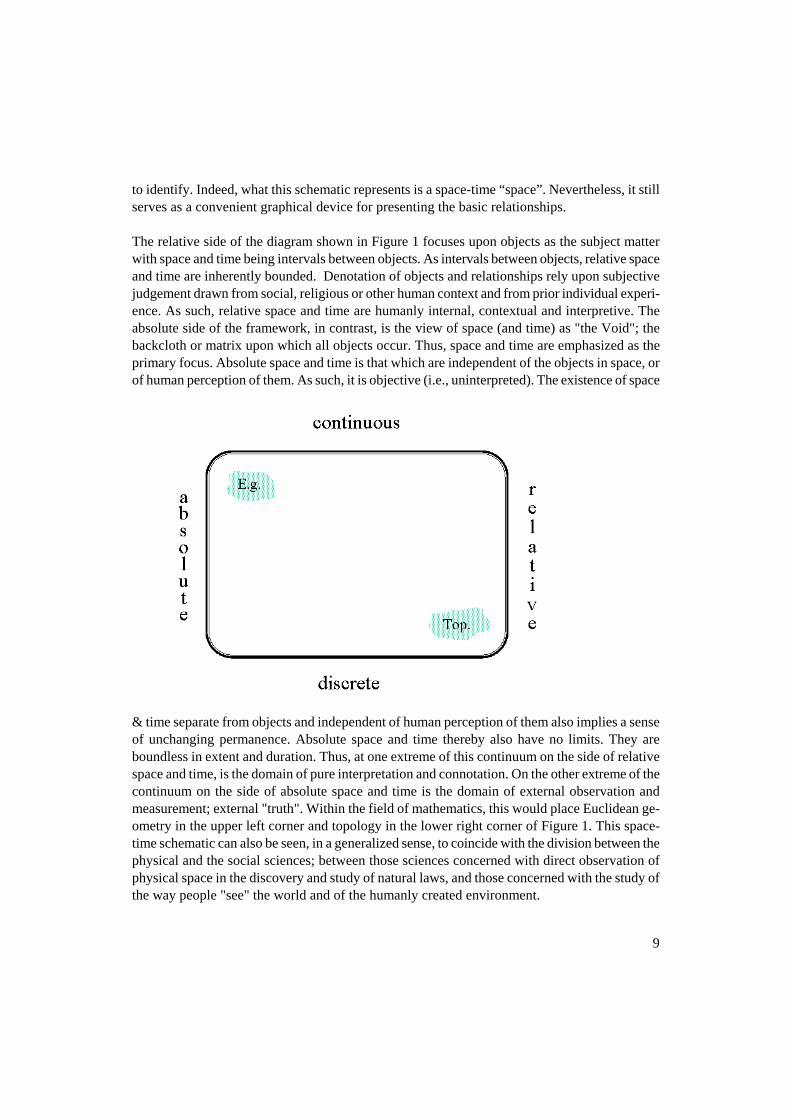
to identify. Indeed, what this schematic represents is a space-time “space”. Nevertheless, it still serves as a convenient graphical device for presenting the basic relationships. The relative side of the diagram shown in Figure 1 focuses upon objects as the subject matter with space and time being intervals between objects. As intervals between objects, relative space and time are inherently bounded. Denotation of objects and relationships rely upon subjective judgement drawn from social, religious or other human context and from prior individual experi-ence. As such, relative space and time are humanly internal, contextual and interpretive. The absolute side of the framework, in contrast, is the view of space (and time) as "the Void"; the backcloth or matrix upon which all objects occur. Thus, space and time are emphasized as the primary focus. Absolute space and time is that which are independent of the objects in space, or of human perception of them. As such, it is objective (i.e., uninterpreted). The existence of space

& time separate from objects and independent of human perception of them also implies a sense of unchanging permanence. Absolute space and time thereby also have no limits. They are boundless in extent and duration. Thus, at one extreme of this continuum on the side of relative space and time, is the domain of pure interpretation and connotation. On the other extreme of the continuum on the side of absolute space and time is the domain of external observation and measurement; external "truth". Within the field of mathematics, this would place Euclidean ge-ometry in the upper left corner and topology in the lower right corner of Figure 1. This space-time schematic can also be seen, in a generalized sense, to coincide with the division between the physical and the social sciences; between those sciences concerned with direct observation of physical space in the discovery and study of natural laws, and those concerned with the study of the way people "see" the world and of the humanly created environment.

9

10

Among the sciences, the physical sciences such as physics and chemistry can be seen as being farthest toward the absolute side of this absolute-relative continuum in their emphasis on the understanding of external reality (and occupying the entire range on the vertical axis, from dis-crete to continuous), progressing toward the relative view somewhere in the middle is geography, as both a physical and a social science, then the social sciences including sociology and econom-ics, with their emphasis on human-created environments and institutions. Psychology would be farthest toward the relative side of this progression, with an emphasis on pure human interpreta-tion and perceptions of reality. Art would certainly occupy the left side of the framework to about the midpoint, representing art forms and styles from those with the intent of faithfully represent-ing reality, to highly abstract forms. Sack had previously provided a similar description (Sack 1980). Analysis of space-time processes - A new era As seen from the above discussion, varying views of space and time are highly interrelated and highly interdependent: “Space is a still of time, while time is space in motion. The two taken together constitute the totality of the ordered relationships characterizing objects and their dis-placements.” (Piaget 1969 p. 2). Time takes on a unique importance in understanding environ-mental space-time processes in that time is inherent in causality. In order to make a causal asso-ciation (as opposed to the perception simply of a chance sequence in a tangle of events) we must establish a conceptual link between events as causes and effects by explaining the occurrence of latter events in terms of former ones. As part of the process of deriving conclusions and thereby learning about our environment, we project forward and backward in time, selecting, grouping and seriating events. This process allows various combinations to be compared, from causes to the effects, until we arrive at a solution that agrees with all the series we have mentally con-structed. Time relates to grouping information in two ways: First, properties of the patterns of movement, per se, define how moving objects will be grouped. For example, if we see a group of objects moving in unison, we see them as a single entity. This is called the Gestalt Law of Common Fate (Kosslyn and Koenig 1992). Second, a specific pattern of movement that tends to happen repeat-edly in sequence will also be viewed as a unit. This is how we can recognize the beginnings of the spread of disease within a community, even though the individual cases come and go as con-tagion is passed from one person to another. Such patterns of movement can also help to identify such “objects,” or space-time groupings. Perhaps the best-known efforts within the field of geography that made explicit use of time as a variable in the study of spatial processes are Hägerstrand's models of diffusion and Time Geogra-phy (Hägerstrand 1967; Pred 1977; Parkes and Thrift 1980). Diffusion models focus on the over-all pattern of specific natural or cultural phenomena as change spreads through space over the passage of time. The "theory of diffusion" has been applied to a diverse range topics, including agricultural innovation, the spread of political unrest, and the spread of AIDS (Parkes and Thrift 1980; Gould 1993). Time Geography deals with complex space-time phenomena by reducing

11

space-time patterns to the individual level, observing paths of individuals through space and time and their interactions. Although Time Geography received much attention, and even excitement, from the early 1970's to the early 1980's, it has since fallen into relative disuse. Certainly, this relative disuse is not the result of a decreased need for space-time analysis. In retrospect, two reasons, encountered in sequence, can be cited for the decline. First, there was a lack of time series data, particularly in digital form, to empirically test many space-time models. This was perhaps most true in the area of social and economic processes. Now that the data are available, the primary problem has be-come how to appropriately represent these data within computer databases so that the space-time patterns and relationships inherent in these data can be effectively uncovered. This gets us back to the issue of the development of effective space-time database models. From the above discussion, what is needed is a multi-representation that allows both relative (interpre-tive) and absolute (measured), continuous and discrete views of the data to coexist simultane-ously within the database. Since the temporal dimension is similar to, but distinct in character from space, the temporal dimension cannot be represented simply as an extension of space, but rather represented in a way that maintains its distinct characteristics. There are efforts ongoing to develop such data models (Mennis and Peuquet 1999). Nevertheless, because of the necessity to rethink the approach to modeling geographic databases at a “first principles” level, much work remains to be done. References Akhundov, M.D. (1986). Conceptions of Space and Time: Sources, Evolution, Directions. Cambridge, Mass., The MIT Press. Aveni, A.F. (1989). Empires of Time: Calendars, Clocks, and Cultures. New York, Basic Books, Inc. Couclelis, H. (1993). Location, Place, Region, and Space. Geography's Inner Worlds: Pervasive Themes in Contemporary American Geography. R.F. Abler, M.G. Marcus and J.M. Olson. New Brunswick, N.J., Rutgers University Press: 215-233. Downs, R. and D. Stea (1973). Image and Environment. Chicago, Aldine. Galison, P.L. (1985). “Minkowski's Space-Time: From Visual Thinking to the Absolute World.” His-torical Studies in the Physical Sciences 10: 85-121. Gleick, J. (1987). Chaos: Making a New Science. New York, Viking Press. Golledge, R. and G. Rushton (1976). Fundamental Conflicts and the Search for Geographical Knowl-edge. A Search for Common Ground. P. Gould and G. Olsson. London, Pion: 11-23. Gould, P. (1993). The Slow Plague: A Geography of the AIDS Pandemic. Cambridge, MA, Blackwell. Hägerstrand, T. (1967). Innovation Diffusion as a Spatial Process. Chicago, Ill., The University of Chicago Press. Hazelton, N.W.J., F.J. Leahy, et al. (1990). On the Design of Temporally-Referenced, 3-D Geographi-cal Information Systems: Development of/ Four-Dimensional GIS. GIS/LIS '90 Proceedings.

12

Kosslyn, S.M. and O. Koenig (1992). Wet Mind, The New Cognitive Neuroscience. New York, The Free Press. Langran, G. (1992). Time in Geographic Information Systems. London, Taylor & Francis. Langran, G. and N.R. Chrisman (1988). “A Framework for Temporal Geographic Information.” Car-tographica 25: 1-14. Mennis, J. and D.J. Peuquet (1999). “A Conceptual Framework for Incorporating Cognitive Principles into Geographic Database Representation.” International Journal of Geographical Information Sci-ence forthcoming. Parkes, D. and N. Thrift (1980). Times, Spaces, and Places. New York, John Wiley & Sons. Peuquet, D.J. (1994). “It's About Time: A Conceptual Framework for the Representation of Temporal Dynamics in Geographic Information Systems.” Annals of the Association of American Geographers 84(3): 441-461. Peuquet, D.J. and N. Duan (1995). “An event-based spatiotemporal data model (ESTDM) for temporal analysis of geographical data.” International Journal of Geographical Information Systems 9(1): 7-24. Piaget, J. (1969). The Child's Conception of Time. New York, Basic Books, Inc. Pred, A. (1977). “The Choreography of Existence: Comments on Hagerstrand's Time Geography and its Usefulness.” Economic Geography 53: 207-221. Sack, R. (1980). Conceptions of Space in Social Thought: A Geographic Perspective. Minneapolis, MN, University of Minnesota Press. Sider, D. (1981). The Fragments of Anaxagoras. Meisenheim am Glan, Hain. Worboys, M. (1994). “A Unified Model for Spatial and Temporal Information.” The Computer Jour-nal 37(1): 26-33. Young, M. (1988). The Metronomic Society: Natural Rhythms and Human Timetables. Cambridge, Mass., Harvard University Press.

The role of geographic visualisation and knowledge discovery in spatio-temporal data modelling Monica Wachowicz Wageningen UR Centre for Geo-Information 1. Introduction One of the most common findings in literature is that time is just one more dimension to be added to the spatial dimension. This perspective is indeed the underlying rationale behind most of the implementations of spatial and temporal data models using relational or object-oriented database architectures. However, the synergy of space and time requires "spatio-temporal concepts" that represent space-time dynamics (for example, moving objects and change) and the human cognition of a knowledge domain (for example, distinction between observed spatio-temporal data and derived knowledge). The join between space and time dimensions is inadequate for representing space and time in database models. Mainly because this will result in a database model that represents the spatial dimension in the same manner as the time dimension, and as a result, it may only capture time-referenced sequences (snap-shots) of spatial data. The Chorochronos Research Network is among the first research initiatives on designing spatio-temporal databases based on spatio-temporal concepts (Chorochronos 1999). In this network, scientists have been emphasising the importance of having a better understanding of spatio-temporal concepts for developing spatio-temporal database models, spatio-temporal operators (e.g. meet, approach), and spatio-temporal user interfaces. One of the main conse-quences of taking on this perspective is that it will allow the representation of states, events, and episodes within an integrated spatio-temporal database model. A state represents a ver-sion of what we know about an entity in a given moment. An event is the moment in time an occurrence, action, or observation takes place. Events and states are also part of a process of change caused by the passage of time. In this process, an episode is the length of time during which change occurs, a state exists, or an event lasts. Consequently, spatio-temporal data modelling is about explaining a knowledge domain using modelling abstractions such as states, events, and episodes. This requires an understanding of the space-time concepts that are used by different experts in the knowledge domain. It also requires the identification of the modelling abstractions (i.e. states, events, and episodes) that can be used for representing them in a spatio-temporal data model. The key issue here is to understand the spatial, temporal, and thematic aspects of a knowledge domain in relation to these modelling abstractions. This is not a trivial task considering the spatio-temporal data sets being generated today, with remotely sensed data from Earth Observation systems alone projected to yield 50 gigabytes of data per hour.

13

From a user perspective, it is essential to explore very large data sets for finding patterns and processes of change in such a way that it provides a dynamic data modelling approach to-wards the identification and interpretation of states, events, and episodes. One way of achiev-ing this objective is by the development and integration of exploratory data analysis and visu-alisation methods. Towards this end, this paper focuses on methods associated with the ex-panding fields of Geographical Visualisation (GVis) and Knowledge Discovery in databases (KDD). GVis has been defined as 'a process, part mental and part concrete (involving human visual thinking, computer data manipulation, and human computer interaction), in which vast quantities of geo-referenced information are sifted and manipulated in the search for patterns and relationships' (MacEachren et al. 1999, p. 313). A primary focus of GVis research over the last decade has been the role of highly interactive tools in facilitating identification and interpretation of patterns and relationships in complex data. The development of KDD coincides with an exponential increase in data generated by and available to science, government, and industry, particularly data generated in digital form. The term "knowledge discovery in databases" was coined in 1989 in an effort to distinguish between the application of data mining algorithms designed to extract pattern from data and the overall process within in which data mining is a step in extracting knowledge from these patterns (Fayyad et al. 1996). Several KDD methods have emerged from the literature and they differ in the conceptualisations developed, reflecting their separate developments in the fields such as database systems, machine learning, statistics, and artificial intelligence (Brachman and Anand 1996, Chen et al. 1996, Ester et al. 1995). KDD has been defined as 'the non-trivial process of identifying valid, novel, potentially useful, and ultimately under-standable patterns in data' (Fayyad et al. 1996, p.6). In the next sections, we summarise the main concepts used for representing space and time in data models. Our focus shifts from modelling abstractions used for storing spatio-temporal data into databases to modelling abstractions for discovering patterns and validating process of change in spatio-temporal databases. This review provides a basis from which we then explore the commonality of goals and potential integration of GVis and KDD methods for developing spatio-temporal data models. 2. Concepts of Space and Time

Time and the way it is handled has a lot to do with structuring space. E.Hall, The Hidden Dimension

Despite having interrelated aims, research in temporal and spatial database models has pre-dominantly developed independently. Langran (1992a) has coined the term "dimensional dominance" to illustrate how our discernment of space and time has been influenced by space-dominant and time-dominant conceptual modelling.

Space-Dominant Data Models The space-dominant models focus on the spatial representation of entities based on the geo-metric and thematic properties of those entities. The attention is given to the spatial model as an ensemble of entities in a geographic space and not so much to an entity itself. The spatial model is usually a layer that can combine a variety of themes and efficiently be used for stor-ing and processing spatial data. Fischer (1997, p. 301) points out: "The idea that the world

14

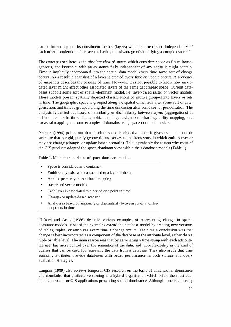
can be broken up into its constituent themes (layers) which can be treated independently of each other is endemic … It is seen as having the advantage of simplifying a complex world." The concept used here is the absolute view of space, which considers space as finite, homo-geneous, and isotropic, with an existence fully independent of any entity it might contain. Time is implicitly incorporated into the spatial data model every time some sort of change occurs. As a result, a snapshot of a layer is created every time an update occurs. A sequence of snapshots describes the passage of time. However, it is not possible to know how an up-dated layer might affect other associated layers of the same geographic space. Current data-bases support some sort of spatial-dominant model, i.e. layer-based raster or vector models. These models present spatially depicted classifications of entities grouped into layers or sets in time. The geographic space is grouped along the spatial dimension after some sort of cate-gorisation, and time is grouped along the time dimension after some sort of periodisation. The analysis is carried out based on similarity or dissimilarity between layers (aggregations) at different points in time. Topographic mapping, navigational charting, utility mapping, and cadastral mapping are some examples of domains using space-dominant models. Peuquet (1994) points out that absolute space is objective since it gives us an immutable structure that is rigid, purely geometric and serves as the framework in which entities may or may not change (change- or update-based scenario). This is probably the reason why most of the GIS products adopted the space-dominant view within their database models (Table 1). Table 1. Main characteristics of space-dominant models.

Space is considered as a container Entities only exist when associated to a layer or theme Applied primarily in traditional mapping Raster and vector models Each layer is associated to a period or a point in time Change- or update-based scenario Analysis is based on similarity or dissimilarity between states at differ-

ent points in time

Clifford and Ariav (1986) describe various examples of representing change in space-dominant models. Most of the examples extend the database model by creating new versions of tables, tuples, or attributes every time a change occurs. Their main conclusion was that change is best incorporated as a component of the database at the attribute level, rather than a tuple or table level. The main reason was that by associating a time stamp with each attribute, the user has more control over the semantics of the data, and more flexibility in the kind of queries that can be used for retrieving the data from a database. They also argue that time stamping attributes provide databases with better performance in both storage and query evaluation strategies. Langran (1989) also reviews temporal GIS research on the basis of dimensional dominance and concludes that attribute versioning is a hybrid organisation which offers the most ade-quate approach for GIS applications presenting spatial dominance. Although time is generally

15

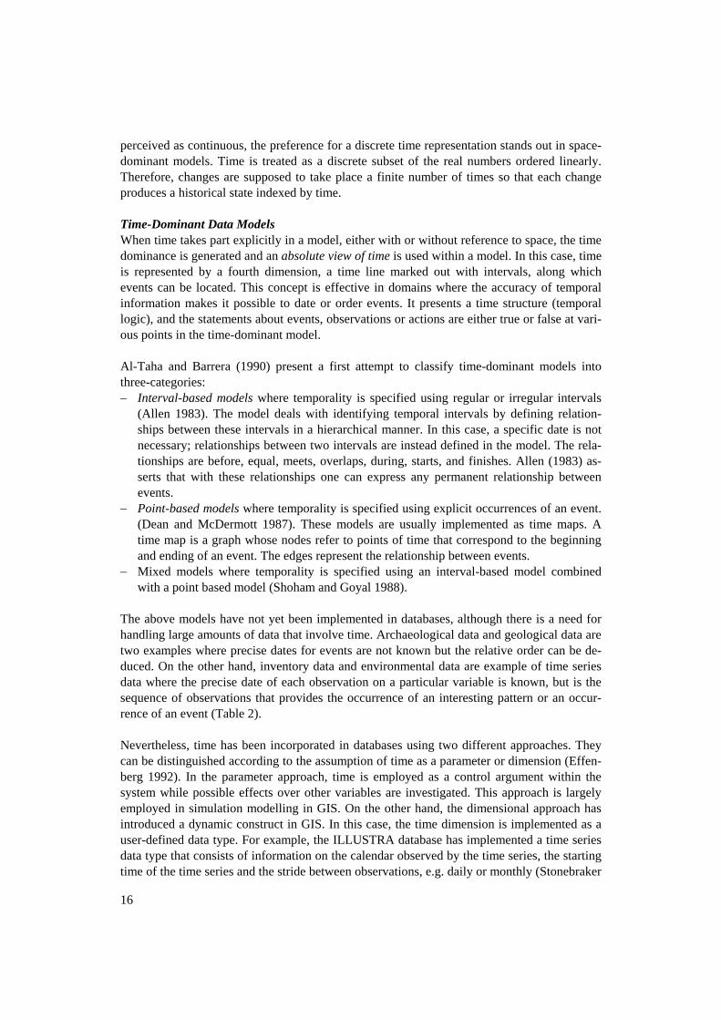
perceived as continuous, the preference for a discrete time representation stands out in space-dominant models. Time is treated as a discrete subset of the real numbers ordered linearly. Therefore, changes are supposed to take place a finite number of times so that each change produces a historical state indexed by time. Time-Dominant Data Models When time takes part explicitly in a model, either with or without reference to space, the time dominance is generated and an absolute view of time is used within a model. In this case, time is represented by a fourth dimension, a time line marked out with intervals, along which events can be located. This concept is effective in domains where the accuracy of temporal information makes it possible to date or order events. It presents a time structure (temporal logic), and the statements about events, observations or actions are either true or false at vari-ous points in the time-dominant model. Al-Taha and Barrera (1990) present a first attempt to classify time-dominant models into three-categories: − Interval-based models where temporality is specified using regular or irregular intervals

(Allen 1983). The model deals with identifying temporal intervals by defining relation-ships between these intervals in a hierarchical manner. In this case, a specific date is not necessary; relationships between two intervals are instead defined in the model. The rela-tionships are before, equal, meets, overlaps, during, starts, and finishes. Allen (1983) as-serts that with these relationships one can express any permanent relationship between events.

− Point-based models where temporality is specified using explicit occurrences of an event. (Dean and McDermott 1987). These models are usually implemented as time maps. A time map is a graph whose nodes refer to points of time that correspond to the beginning and ending of an event. The edges represent the relationship between events.

− Mixed models where temporality is specified using an interval-based model combined with a point based model (Shoham and Goyal 1988).

The above models have not yet been implemented in databases, although there is a need for handling large amounts of data that involve time. Archaeological data and geological data are two examples where precise dates for events are not known but the relative order can be de-duced. On the other hand, inventory data and environmental data are example of time series data where the precise date of each observation on a particular variable is known, but is the sequence of observations that provides the occurrence of an interesting pattern or an occur-rence of an event (Table 2). Nevertheless, time has been incorporated in databases using two different approaches. They can be distinguished according to the assumption of time as a parameter or dimension (Effen-berg 1992). In the parameter approach, time is employed as a control argument within the system while possible effects over other variables are investigated. This approach is largely employed in simulation modelling in GIS. On the other hand, the dimensional approach has introduced a dynamic construct in GIS. In this case, the time dimension is implemented as a user-defined data type. For example, the ILLUSTRA database has implemented a time series data type that consists of information on the calendar observed by the time series, the starting time of the time series and the stride between observations, e.g. daily or monthly (Stonebraker

16

and Moore 1996). This allows the users to query a database using temporal operators such as begin, finish, and overlap. Table 2. Main characteristics of the time-dominant models.

Time is considered as a time line Events are associated to a time line Applied in archaeology, geology, and environmental sciences Interval, point, and mixed models Space is where an event takes place Event-based scenario Analysis is based on the lineage of events

The Relative Space-Time View Both space- and time-dominant data models have influenced research outcomes since the early 1980s. Armstrong (1988) has defined eight possible combinations of changes or updates that can occur in vector-based models. For each possible update procedure, a change is asso-ciated with the geometry, topology, and thematic properties of an entity in space. Kucera (1996) has also advocated the need for developing data-driven update procedures in GIS; procedures based on where and when the changes occur. However, the relative view of space and time is also of the most fundamental importance for representing space and time in database models. The concept of relative space is more general and empirically more useful than the concept of absolute space. Jammer (1969, p. 23) defines relative space as "an ordering relation that holds between bodies and determines their relative positions … a system of interconnected relations." The profound implication is that any rela-tion defined on a set of entities creates space. In other words, defining a relation automati-cally defines a space. Harvey (1969) provides an excellent review of the two perspectives, absolute and relative space. The concept of absolute space overemphasises the absolute loca-tion of entities within a spatial data model. In contrast, relative space focuses on the relative location among entities and events. The relativistic point of view is usually associated with studies of forms, patterns, functions, rates, and diffusion processes. A complementary concept is relative time - time measured in relation to something, not con-strained to a single dimensional axis. Cyclical time - the repeating of a day, week, or year - is an example of relative time. In absolute time, 13 August 1998 cannot be repeated. But in relative time, Thursdays keep returning. Most questions about change will be understood from this perspective (Ornstein 1969). Relative time is subjective since it assumes a flexible structure that is more topological in the sense that is defined in terms of relationships between events. For example, Frank (1994) suggested an ordinal model of time in which an episode is defined according to relativity among events of a time line rather than attaching precise dates for these events. The relative space-time view embraces human activity over the real world that results from studying processes within a knowledge domain. 'A process study seeks to identify the rules which govern spatio-temporal sequences, in such a form that the rules are interpretable in

17

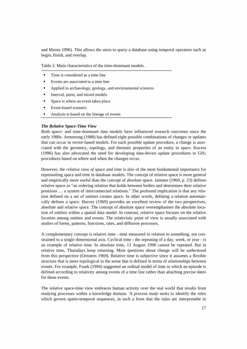
terms of the results of the sequence, in terms of the exogenous variables which influence the sequence, and in terms of the mechanisms by which exogenous and endogenous influences give rise to the results which the sequence itself records' (Dictionary of Human Geography, 1994, p. 478. Table 3 summarises the main characteristics encountered in the relative space-time view in data modelling. Table 3. Main characteristics of the relative space-time view.

Space and time are considered as coexistence (connection or together-ness) relationships between states and events

Neither space nor time exists independently Applied in studies of forms, patterns, functions, rates, and diffusion Topological models May involve non-Euclidean space or non-linear time Process-based scenario Analysis based on a process study

Very few attempts have been made in applying the relative space-time view within database models. Gatrell (1983) provides some examples of constructing space-time maps based on proximity relations among entities. The examples implement the Multi-Dimensional Scaling (MDS) approach, in which relations are defined by numerical values in a matrix representing perceived distances between entities (main cities in New Zealand) rather than the actual measured distances. Egenhofer and Al-Taha (1992) have also carried out a study of gradual changes of topological relationships such as translation, scaling, and rotation. The changes have been formalised using eight binary topological relationships for two spatial regions. The eight binary topological relations are depicted in the closest topological relationship graph showing the links between gradual changes in topology. Choosing a conceptual view for representing space and time in database models Harvey (1969) argues that we have frequently taken a particular conceptual view (i.e. abso-lute view or relative view) for constructing a data model without examining the rationale for such a choice. After all, we should not discriminate one over another. They are complemen-tary. The absolute view requires some sort of measurements referenced to a constant base, implying non-judgmental observation. The relative view, on the other hand, involves interpre-tation of processes and the flux of changing patterns within a knowledge domain. However, a question still remains about integrating absolute and relative views. How can we have both perspectives placed in the same spatio-temporal database model? TEMPEST (Temporal Geographic Information System), proposed by Peuquet (1994), is the first effort towards the integration of space- and time-dominant data models in GIS. 'Location in time becomes the primary organisational basis for recording change. The sequence of events through time, representing the spatio-temporal manifestation of some process, is noted via a time-line; i.e., a line through the single dimension of time instead of a two-dimensional surface over space …. Such a line, then, represents an ordered progression through time of

18

known changes from some known starting date or moment to some known, later, point in time.' (Peuquet and Wentz, 1994, p. 495). Few examples are available for illustrating the attempts at designing a spatio-temporal data-base model using both relative and absolute views of space and time. Wachowicz (1999) describes a spatio-temporal database model for the integration of both views. The approach is based on object-oriented analysis and design methods, which can provide the modelling ab-stractions to capture the complexity of space-time interaction of events and changes within a lifespan of an entity. The Time Geography (Pred 1977, Hagerstrand 1975) framework is also used to capture the absolute location in space and time of an entity, as well as the relative location of events and changes that have occurred in a lifespan of this entity. The potential application of this spatio-temporal database model is shown in a wide range of knowledge domains such as political boundary record maintenance (historical data sets), disease inci-dence rate analysis in epidemics (diffusion data), and environmental studies of climate change (time-series data). Another example is the application of Time Geography for simulating an individual's daily shopping behaviour within a GIS (Makin 1992). The results show how space and time constraints on people's shopping movements affect shops' potential earning and profits. Makin explores the potential of using a database to structure spatial relationships according to which routes are accessible to each other, and where the buildings are located on the route network. The next sections describe two emerging research fields related to the integration of relative and absolute views of space and time within spatio-temporal data models. Each section be-gins with a brief description of the research field then examines its impact on designing a dynamic knowledge construction process for spatio-temporal data modelling.

3. Geographic Visualisation - GVis Most GVis research has focused on overcoming the problems involved in applying the latest technology for the creation of visual representations of spatial (and spatio-temporal) data (Card et al. 1999). Visual representations have been developed with the use of computer-supported and interactive tools, with emphasis on the analysis of multidimensional data, the visualisation of novel sorts of data and the quality of the graphics display. Some examples of visualisation methods are 3D scattterplots (Cleveland and McGill 1988), map animation (Openshaw 1994, Mitas et al. 1997), parallel coordinate plots (Inselberg 1997), and graphics techniques for large-scale sets of data (Mihalisin et al. 1991, Eick 1994). Our focus here is a view of GVis as a process, part mental and part concrete (involving human visual thinking, computer data manipulation, and human computer interaction), in which a very large number of variables (dimensions) of spatio-temporal data are explored using visual representations (MacEachren et al. 1999). Among the first process oriented perspectives is DiBiase's (1990) characterisation of a GVis process as consisting of four stages, which are exploration, confir-mation, synthesis, and presentation. In this case, the goal of a map is to stimulate a hypothesis rather than to portray a message. Knowledge is to some extent constructed by the user based on the visual display of information. In a GVis process, visual representations are structures that have an effect on how we “see” and “interact” with data using both vision and information processing cognition. Visual rep-resentations allow us to derive meaning from visual displays and interrelate them with differ-

19

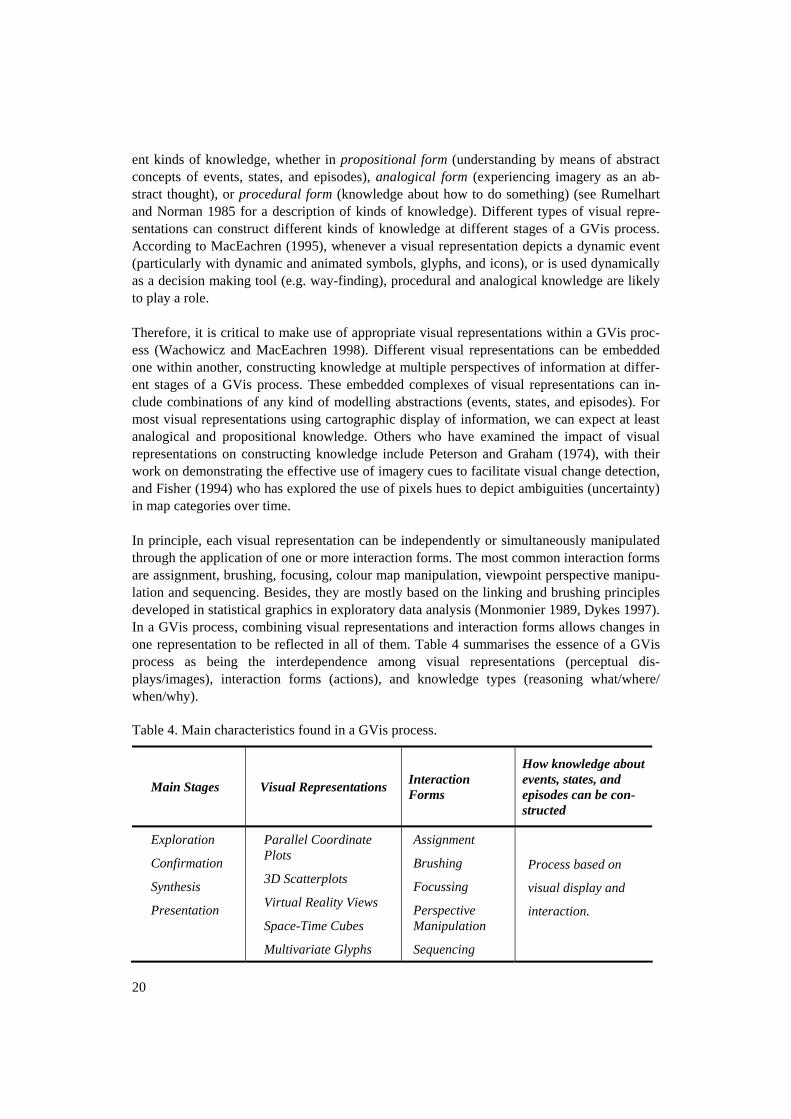
ent kinds of knowledge, whether in propositional form (understanding by means of abstract concepts of events, states, and episodes), analogical form (experiencing imagery as an ab-stract thought), or procedural form (knowledge about how to do something) (see Rumelhart and Norman 1985 for a description of kinds of knowledge). Different types of visual repre-sentations can construct different kinds of knowledge at different stages of a GVis process. According to MacEachren (1995), whenever a visual representation depicts a dynamic event (particularly with dynamic and animated symbols, glyphs, and icons), or is used dynamically as a decision making tool (e.g. way-finding), procedural and analogical knowledge are likely to play a role. Therefore, it is critical to make use of appropriate visual representations within a GVis proc-ess (Wachowicz and MacEachren 1998). Different visual representations can be embedded one within another, constructing knowledge at multiple perspectives of information at differ-ent stages of a GVis process. These embedded complexes of visual representations can in-clude combinations of any kind of modelling abstractions (events, states, and episodes). For most visual representations using cartographic display of information, we can expect at least analogical and propositional knowledge. Others who have examined the impact of visual representations on constructing knowledge include Peterson and Graham (1974), with their work on demonstrating the effective use of imagery cues to facilitate visual change detection, and Fisher (1994) who has explored the use of pixels hues to depict ambiguities (uncertainty) in map categories over time. In principle, each visual representation can be independently or simultaneously manipulated through the application of one or more interaction forms. The most common interaction forms are assignment, brushing, focusing, colour map manipulation, viewpoint perspective manipu-lation and sequencing. Besides, they are mostly based on the linking and brushing principles developed in statistical graphics in exploratory data analysis (Monmonier 1989, Dykes 1997). In a GVis process, combining visual representations and interaction forms allows changes in one representation to be reflected in all of them. Table 4 summarises the essence of a GVis process as being the interdependence among visual representations (perceptual dis-plays/images), interaction forms (actions), and knowledge types (reasoning what/where/ when/why). Table 4. Main characteristics found in a GVis process.

Main Stages Visual Representations Interaction Forms

How knowledge about events, states, and episodes can be con-structed

Exploration

Confirmation

Synthesis

Presentation

Parallel Coordinate Plots

3D Scatterplots

Virtual Reality Views

Space-Time Cubes

Multivariate Glyphs

Assignment

Brushing

Focussing

Perspective Manipulation

Sequencing

Process based on

visual display and

interaction.

20

4. Knowledge Discovery Knowledge discovery in databases (KDD) has been defined as “the non-trivial process of identifying valid, novel, potentially useful, and ultimately understandable patterns in data” (Fayyad et al. 1996, p.6). The development of KDD coincides with an exponential increase in digital spatio-temporal data generated by and available to science, government, and industry. Several KDD methods have recently emerged from the literature and they differ in the con-ceptualisations developed in separate fields such as database systems, machine learning, sta-tistics, and artificial intelligence. While several authors have proposed different delineations of a KDD process, the five-stage process proposed by Fayyad et al. (1996) has been generally accepted. A KDD process is described as consisting of: − Data Selection: having two subcomponents: (a) developing an understanding of the prob-

lem domain and (b) creating a target data set from the universe of available data. − Preprocessing: including data cleaning and transformations, such as dealing with missing

values, dimensionality reduction, and errors. − Data Mining: having two subcomponents, which are (a) choosing the data mining task

(classification, clustering, summarisation), and (b) choosing the algorithms to be used in performing the tasks.

− Interpretation/Evaluation: understanding of the mined patterns, potentially leading to a repeat of earlier steps.

Brachman and Anand (1996) have emphasised that in a KDD process, data mining is an in-tensive stage, consisting of complex interactions between a human and a large database. Typical tasks for data mining are clustering, classification, generalisation and prediction, for which researchers have been developing data mining methods using heuristics, bounded-error approximation and approximate algorithms. Ramakrishman and Grama (1999) have presented a taxonomy in which data mining methods have been classified according to four recurrent perspectives on how knowledge can be constructed. They are induction, compression, query-ing, and approximation. The most common perspective is induction with its origin in AI and machine learning, in which data mining methods are based on “learning-from-examples” concept. Hunt, Martin, and Stone (1966) were among the first scientists to study the learning-from-examples con-cept. Their methodology was based on incrementally constructing decision trees that dis-criminate observations of different classes. Recently, in the database community, the attrib-ute-oriented induction method (Cai, Cercone and Han 1991, Han and Fu 1995) has been de-veloped aiming the integration of learning-from-examples methods with database operations (e.g. group by) in order to extract generalised rules from a data set and detect high-level data irregularities. Basically, attribute-oriented induction method is based on ascending a generali-sation hierarchy and summarising the general relationships between attributes at higher con-cept levels. A generalisation hierarchy can explicitly be specified by a domain expert (e.g. agricultural land use) or can be generated automatically. Several authors have investigated attribute-oriented induction methods for extracting generalisation hierarchies for spatial data (Wang et al. 1997, Han et al. 1997). Moreover, this approach has also been explored for the extraction of different kinds of rules, including characteristic rules, discriminant rules, cluster description rules, and multi-level association rules (Fayyad et al. 1996).

21

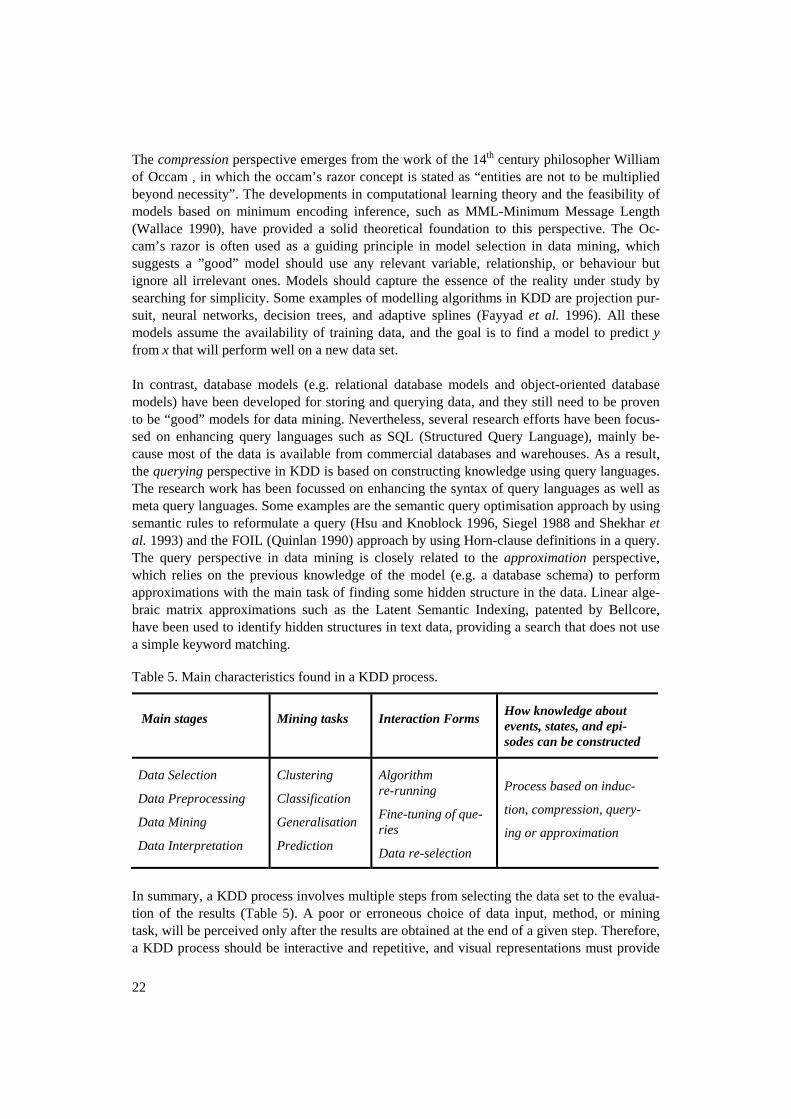
The compression perspective emerges from the work of the 14th century philosopher William of Occam , in which the occam’s razor concept is stated as “entities are not to be multiplied beyond necessity”. The developments in computational learning theory and the feasibility of models based on minimum encoding inference, such as MML-Minimum Message Length (Wallace 1990), have provided a solid theoretical foundation to this perspective. The Oc-cam’s razor is often used as a guiding principle in model selection in data mining, which suggests a ”good” model should use any relevant variable, relationship, or behaviour but ignore all irrelevant ones. Models should capture the essence of the reality under study by searching for simplicity. Some examples of modelling algorithms in KDD are projection pur-suit, neural networks, decision trees, and adaptive splines (Fayyad et al. 1996). All these models assume the availability of training data, and the goal is to find a model to predict y from x that will perform well on a new data set. In contrast, database models (e.g. relational database models and object-oriented database models) have been developed for storing and querying data, and they still need to be proven to be “good” models for data mining. Nevertheless, several research efforts have been focus-sed on enhancing query languages such as SQL (Structured Query Language), mainly be-cause most of the data is available from commercial databases and warehouses. As a result, the querying perspective in KDD is based on constructing knowledge using query languages. The research work has been focussed on enhancing the syntax of query languages as well as meta query languages. Some examples are the semantic query optimisation approach by using semantic rules to reformulate a query (Hsu and Knoblock 1996, Siegel 1988 and Shekhar et al. 1993) and the FOIL (Quinlan 1990) approach by using Horn-clause definitions in a query. The query perspective in data mining is closely related to the approximation perspective, which relies on the previous knowledge of the model (e.g. a database schema) to perform approximations with the main task of finding some hidden structure in the data. Linear alge-braic matrix approximations such as the Latent Semantic Indexing, patented by Bellcore, have been used to identify hidden structures in text data, providing a search that does not use a simple keyword matching. Table 5. Main characteristics found in a KDD process.

Main stages Mining tasks Interaction Forms How knowledge about events, states, and epi-sodes can be constructed

Data Selection

Data Preprocessing

Data Mining

Data Interpretation

Clustering

Classification

Generalisation

Prediction

Algorithm re-running

Fine-tuning of que-ries

Data re-selection

Process based on induc-

tion, compression, query-

ing or approximation

In summary, a KDD process involves multiple steps from selecting the data set to the evalua-tion of the results (Table 5). A poor or erroneous choice of data input, method, or mining task, will be perceived only after the results are obtained at the end of a given step. Therefore, a KDD process should be interactive and repetitive, and visual representations must provide

22

feedback to earlier results of a data mining task. The successful applications of KDD will be defined by the strength of the human computer interaction and the GVis methods it supports, especially those with an emphasis on developing visual representations of information and operations to acting on that information. The fundamental goal is to convert data to a visual form that exploits human skills in perception and interactive.

5. Developing a spatio-temporal data model based on GVis and KDD processes It is clear that GVis and KDD processes share perspectives related to both goals and ap-proach. For each process, a primary goal is to find, relate, and interpret interesting, meaning-ful, and unknown features in spatio-temporal data sets. In both cases, the knowledge con-struction process is considered as a complex process, and researchers have recognised the important role of the user domain expert in understanding the process and in interpreting the results. In addition, methods in GVis and KDD emphasise iteration as central to their effec-tive application. Neither a single visual representation of a spatio-temporal data set nor a single data mining run is expected to result in profound insight. It is only by repeated applica-tion of methods, with systematic changes in operations, that a coherent picture is expected to emerge. Many people do not realise that spatio-temporal database models have been treated as static representations, with its own conventions, procedures and limitations. The classification proc-ess in which two assumptions are taken gives the most representative example. First, classes are like containers, with objects either inside or outside. Second, objects in the same class must have the same properties. One of the consequences of this reality is the proliferation of database operations to perform data capture, editing, query, and display, but having limited capabilities to perform exploratory data analysis In contrast, a bayesian classification in a KDD process is an example of employing statistical theory to obtain membership classifications of objects to multiple classes at the same time. Therefore, objects in the same class do not have the same properties. They are grouped based on a membership criterion (or criteria). The classification results can provide a spatio-temporal representation of how the data can be distributed into classes in a way that was not previously conceived for a spatio-temporal data model. It can also be used to predict new classes for a spatio-temporal data model. Geographic visualisation involves much more than just enabling users to ‘see’ spatio-tempo-ral data. GVis plays an important role as the means to communicate different decisions taken in the modelling process and share information in a collaborative environment. In fact, GVis acts directly to perform exploratory visual analysis based on this information. GVis will sup-port information search, analysis, communication and system control operations using an interactive user interface of a spatio-temporal database model as well the contents of the da-tabase. 6. Conclusions The main objective of this paper has been to disclose the value of integrating GVis and KDD methods and their relevance to spatio-temporal data modelling. The strength of the develop-ment and integration of GVis and KDD methods lie in the powerful integrated system that they can provide for spatio-temporal data modelling. A system from which to store, explore,

23

and evaluate very large amounts of data, and subsequently understand and communicate this understanding. Particularly when applied to environmental data, designing an integrated GVis-KDD system is a research challenge. The forthcoming tools will facilitate pattern notic-ing, whether this pattern is used for steering data mining, identifying, comparing, and analys-ing entities, or trying to link entities to a real-world phenomenon. The key goal is to find relationships among entities in thematic, temporal, or space within a single transparent envi-ronment that is intuitive and supportive of the heuristics of the domain expert while defining a flexible, adaptive control structure for algorithmic process and graphic user interface - the ideal paradigm for the GVis and KDD integration for supporting spatio-temporal data model-ling. The users will not be required to know exactly the data and its corresponding database model before beginning the process of query specification. Most of the current query interfaces al-low a user to issue queries in a one-by-one basis, with no possibility to express vague, uncer-tain or ambiguous queries neither to incrementally refine a query nor as an effective way to find interesting, a priori unknown, patterns of the data. Most importantly, the user obtains no feedback after receiving the results of a query statement, except the resulting data set contain-ing either many data items or no data items, and thus no indication for continuing the search. A pragmatic example is found in retrieving interesting data from environmental databases, in which users are searching for data of test series for significant values, or they might be look-ing for some correlation between multivariate variables for some specific period of time at a geographic region. Since none of the parameters for the query is fixed, it is in general very difficult to find the needed information. The scientists would probably start to specify a query that corresponds to some assumptions and after issuing many refined queries and applying statistical methods to the results, they might find interesting patterns. Interactive query interface tools through which users can dynamically change queries, receive valuable feedback in querying the database, assign data attributes to be visualised to graphical properties, and control the coordination among visualisations derived from different queries, are some examples of envisaged capabilities to support such a dynamic process for spatio-temporal data modelling. The basic premise behind this paper is that offering interactive support is the best way to enable a knowledge construction process using the expertise of specialists for developing spatio-temporal data models. This approach aims to help the expert in the process of interact-ing with a system rather than doing the task for the expert. Introducing exploratory analysis requires a systematic and dynamic spatio-temporal data models for the processes involved in applying the methods developed in GVis and KDD. The approach suggested in this paper relies on a knowledge construction process that reflects not the end result a user would want, and therefore what the model should produce, but rather the actions a user would perform on identified generic steps of a knowledge construction process. This is an important distinction. Existing knowledge engineering focuses on identify-ing what kind of knowledge the spatio-temporal data model needs to reason successfully, whereas our approach focuses on identifying what kind of knowledge a user needs to interact effectively with the model. It is consistent with taking the initiative of enabling users exper-tise, rather than attempting to supplant their expertise.

24

7. References Allen, J.F. (1983). Maintaining knowledge about temporal intervals. Communications of ACM, 26, 832-43. Al-Taha, K.K. and Barrera, R. (1990). Temporal data and GIS: an overview. Proceedings of the GIS/LIS’90 Conference, 1, 244-54. Armstrong, M.P. (1988). Temporality in spatial databases. Proceedings GIS/LIS’88 Conference, 2, 880-90. Cai, Y., Cercone, N. and Han, J. (1991). Attribute-Oriented Induction in relational databases. In Knowledge Discovery in Databases, G. Piatesky-Shapiro and W.J. Frawley, AAAI Press, 213-218. Card, S.K., MacKinlay, J.D., and Shneiderman, B. (1999). Readings in Information Visualisation, Using Vision to Think. Morgan Kaufmann Publishers, Inc. Chen, M., Han, J., and Yu, P.S. (1996). Data Mining: An Overview from a Database Perspective. IEEE Transactions on Knowledge and Data Engineering, 8, 866-883. Chorochronos (1999). Chorochronos: A research network for spatiotemporal database systems. SIGMOD Record, 28(3), 12-21. Cleveland, and McGill, (1988). Dynamic Graphics for Statistics. Clifford, J. and Ariav, G. (1986). Temporal data management: models and systems. In New Direc-tions for Database Systems, Ariav, G. and Clifford, J. (eds), Ablex Publishing, 168-85. Brachman, R.J. and Anand, T. (1996). The Process of Knowledge Discovery in Databases. In: Advances in Knowledge Discovery and Data Mining. U.M Fayyad et al. (eds.) AAAI Press/The MIT Press, 37-57. Dean, T.L. and McDermott, D.V. (1987). Temporal data base management. Artificial Intelligence, 32, 1-55. DiBiase, D. (1990). Visualisation in the Earth Sciences. Earth and Mineral Sciences, Bulletin of the College of Earth and Mineral Sciences, Penn State University, 59(2): 13-18. Dykes, J.A. (1997). Exploring spatial data representation with dynamics graphics. Computers and Geosciences, 23, 345-370. Effenberg, W.W. (1992). Time in spatial information systems, First Regional Conference on GIS Research in Victoria and Tasmania, Victoria. Egenhoffer, M.J. and Al-Taha, K.K. (1992). Reasoning about gradual changes of topological relationships. In Theories and Methods of Spatio-Temporal Reasoning in Geographical Space, Frank, A. et al. (eds), Springer Verlag, 196-219. Eick, S.G. (1994). Data visualisation sliders. Proceedings UIST'94, 119-120. Ester, M., Kriegel, H.P., and Xu, X. (1995). Knowledge Discovery in Large Spatial Databases: Focussing Techniques for Efficient Class Identification. Proceedings International Symposium on Large Databases (SSD'95), Maine. Fayyad, U., Piatestsky-Shapiro, G., and Smyth, P. (1996). From Data Mining to Knowledge Dis-covery: An Overview. In: Advances in Knowledge Discovery and Data Mining. U.M Fayyad et al. (eds.) AAAI Press/The MIT Press, 1- 34. Fisher, P. (1994). Randomisation and sound for the visualisation of uncertain spatial information. In Visualisation in GIS, D.Unwin and H. Heardnshaw (eds), Wiley, 181-185. Fisher, P. (1997). Concepts and paradigms of spatial data. In Geographic Information Research: Bridging the Atlantic, Craglia, M. and Couclelis, H. (eds), Taylor and Francis, 297-307.

25

Frank, A.U. (1994). Qualitative temporal reasoning in GIS – ordered time scales. Proceedings of the SDH’94 Conference,1, 410-30. Gatrell, A. (1983). Distance and Space: A geographical perspective. Clarendon Press. Hagerstrand, T. (1975). Space, time and human conditions. In Dynamic allocation of urban space, Karlqvist et al. (eds), Saxon House, 3-14. Han, J. and Fu, Y. (1995). Discovery of multiple-level associations rules from large databases. Proceedings of the International Conference on Very Large Databases, 430-431. Han, J., Koperski, K. and Stefanovic, N. (1997). GeoMiner: A System Prototype for Spatial Min-ing. Proceedings ACM-SIGMOD 1997, Arizona Harvey, D. (1969). Explanation in Geography, St Martin’s Press. Hsu, C.N. and Knoblock, C.A. (1996). Using Inductive Learning to generate rules for semantic query optimisation. In: Advances in Knowledge Discovery and Data Mining. U.M Fayyad et al. (eds.) AAAI Press/The MIT Press, 425-445. Hunt, E., Marin, J. and Stone, P. (1966). Experiments in induction. New York: Academic Press. Inselberg, A. (1997). Multidimensional Detective. Proceedings IEEE Information Visualisa-tion'97, 100-107. Jammer, M. (1969). Concepts of space. Cambridge, Harward University Press. Kucera, G.L. (1996). Temporal extensions to spatial data models: Final report. US Army Con-struction Engineering Research Laboratory. Langran, G. (1989). A review of temporal database research and its use in GIS applications. Inter-national Journal of GIS, 3(3), 215-32. MacEachren, A.M. (1995). How maps Work: Representation, Visualisation and Design. Guilford Press. MacEachren, A.M., Wachowicz, M., Edsall, R., Haug, D. and Masters, R. (1999). Constructing knowledge from multivariate spatiotemporal data: integrating geographical visualisation with knowledge discovery methods. International Journal of Geographical Information Science,13(4), 311-334. Makin, J. (1992). An object-oriented simulation of a complex geographical system using GIS, MSc dissertationj (unpublished), University of Edinburgh. Mihalisin, T., Timlin, J. and Schwegler, J. 91991), Visualising multivariate functions, data, and distributions. IEEE Computer Graphics and Applications, 11(13), 28-35. Mitas, L., Brown, W.M. and Mitasova, H. (1997). Role of Dynamic Cartography in Simulations of Landscape processes Based on Multivariate Fields. Computer and GeoSciences, 23(4): 437-446.

26

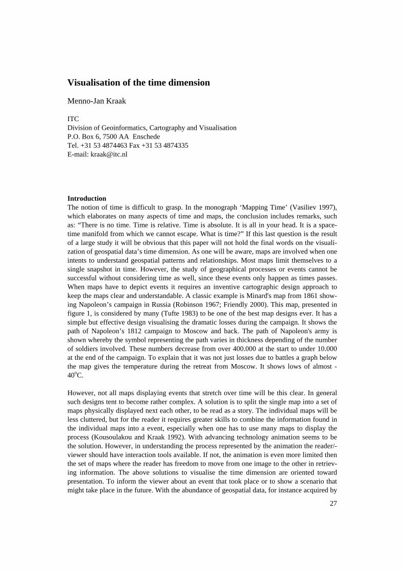
Visualisation of the time dimension Menno-Jan Kraak ITC Division of Geoinformatics, Cartography and Visualisation P.O. Box 6, 7500 AA Enschede Tel. +31 53 4874463 Fax +31 53 4874335 E-mail: kraak@itc.nl Introduction The notion of time is difficult to grasp. In the monograph ‘Mapping Time’ (Vasiliev 1997), which elaborates on many aspects of time and maps, the conclusion includes remarks, such as: “There is no time. Time is relative. Time is absolute. It is all in your head. It is a space-time manifold from which we cannot escape. What is time?” If this last question is the result of a large study it will be obvious that this paper will not hold the final words on the visuali-zation of geospatial data’s time dimension. As one will be aware, maps are involved when one intents to understand geospatial patterns and relationships. Most maps limit themselves to a single snapshot in time. However, the study of geographical processes or events cannot be successful without considering time as well, since these events only happen as times passes. When maps have to depict events it requires an inventive cartographic design approach to keep the maps clear and understandable. A classic example is Minard's map from 1861 show-ing Napoleon’s campaign in Russia (Robinson 1967; Friendly 2000). This map, presented in figure 1, is considered by many (Tufte 1983) to be one of the best map designs ever. It has a simple but effective design visualising the dramatic losses during the campaign. It shows the path of Napoleon’s 1812 campaign to Moscow and back. The path of Napoleon's army is shown whereby the symbol representing the path varies in thickness depending of the number of soldiers involved. These numbers decrease from over 400.000 at the start to under 10.000 at the end of the campaign. To explain that it was not just losses due to battles a graph below the map gives the temperature during the retreat from Moscow. It shows lows of almost -40oC. However, not all maps displaying events that stretch over time will be this clear. In general such designs tent to become rather complex. A solution is to split the single map into a set of maps physically displayed next each other, to be read as a story. The individual maps will be less cluttered, but for the reader it requires greater skills to combine the information found in the individual maps into a event, especially when one has to use many maps to display the process (Kousoulakou and Kraak 1992). With advancing technology animation seems to be the solution. However, in understanding the process represented by the animation the reader/-viewer should have interaction tools available. If not, the animation is even more limited then the set of maps where the reader has freedom to move from one image to the other in retriev-ing information. The above solutions to visualise the time dimension are oriented toward presentation. To inform the viewer about an event that took place or to show a scenario that might take place in the future. With the abundance of geospatial data, for instance acquired by

27

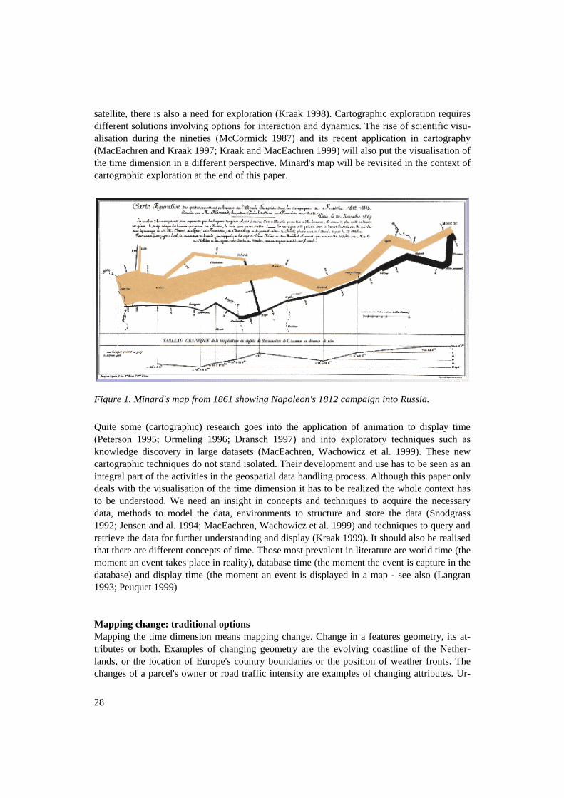
satellite, there is also a need for exploration (Kraak 1998). Cartographic exploration requires different solutions involving options for interaction and dynamics. The rise of scientific visu-alisation during the nineties (McCormick 1987) and its recent application in cartography (MacEachren and Kraak 1997; Kraak and MacEachren 1999) will also put the visualisation of the time dimension in a different perspective. Minard's map will be revisited in the context of cartographic exploration at the end of this paper.

Figure 1. Minard's map from 1861 showing Napoleon's 1812 campaign into Russia.

Quite some (cartographic) research goes into the application of animation to display time (Peterson 1995; Ormeling 1996; Dransch 1997) and into exploratory techniques such as knowledge discovery in large datasets (MacEachren, Wachowicz et al. 1999). These new cartographic techniques do not stand isolated. Their development and use has to be seen as an integral part of the activities in the geospatial data handling process. Although this paper only deals with the visualisation of the time dimension it has to be realized the whole context has to be understood. We need an insight in concepts and techniques to acquire the necessary data, methods to model the data, environments to structure and store the data (Snodgrass 1992; Jensen and al. 1994; MacEachren, Wachowicz et al. 1999) and techniques to query and retrieve the data for further understanding and display (Kraak 1999). It should also be realised that there are different concepts of time. Those most prevalent in literature are world time (the moment an event takes place in reality), database time (the moment the event is capture in the database) and display time (the moment an event is displayed in a map - see also (Langran 1993; Peuquet 1999) Mapping change: traditional options Mapping the time dimension means mapping change. Change in a features geometry, its at-tributes or both. Examples of changing geometry are the evolving coastline of the Nether-lands, or the location of Europe's country boundaries or the position of weather fronts. The changes of a parcel's owner or road traffic intensity are examples of changing attributes. Ur-

28

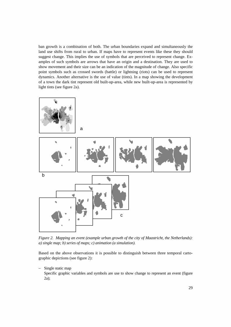
ban growth is a combination of both. The urban boundaries expand and simultaneously the land use shifts from rural to urban. If maps have to represent events like these they should suggest change. This implies the use of symbols that are perceived to represent change. Ex-amples of such symbols are arrows that have an origin and a destination. They are used to show movement and their size can be an indication of the magnitude of change. Also specific point symbols such as crossed swords (battle) or lightning (riots) can be used to represent dynamics. Another alternative is the use of value (tints). In a map showing the development of a town the dark tint represent old built-up-area, while new built-up-area is represented by light tints (see figure 2a).

a

c

b

Figure 2. Mapping an event (example urban growth of the city of Maastricht, the Netherlands): a) single map; b) series of maps; c) animation (a simulation). Based on the above observations it is possible to distinguish between three temporal carto-graphic depictions (see figure 2): − Single static map

Specific graphic variables and symbols are use to show change to represent an event (figure 2a);

29

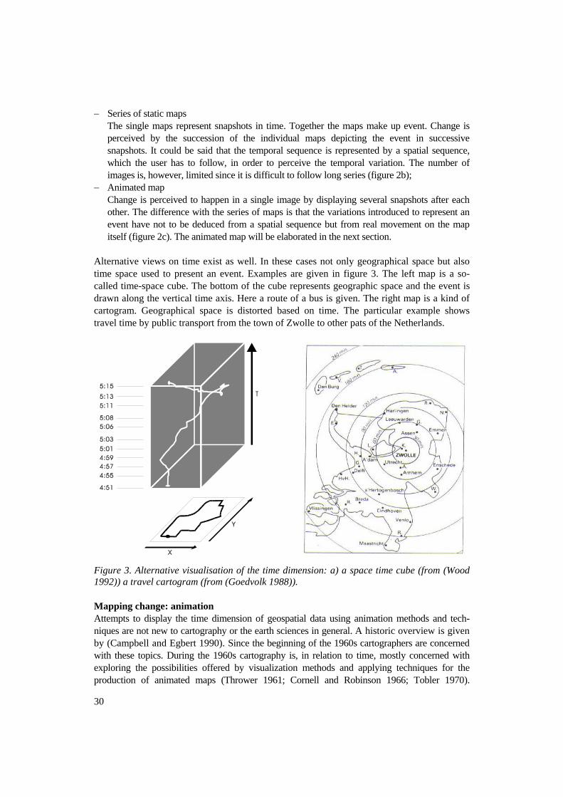
− Series of static maps The single maps represent snapshots in time. Together the maps make up event. Change is perceived by the succession of the individual maps depicting the event in successive snapshots. It could be said that the temporal sequence is represented by a spatial sequence, which the user has to follow, in order to perceive the temporal variation. The number of images is, however, limited since it is difficult to follow long series (figure 2b);

− Animated map Change is perceived to happen in a single image by displaying several snapshots after each other. The difference with the series of maps is that the variations introduced to represent an event have not to be deduced from a spatial sequence but from real movement on the map itself (figure 2c). The animated map will be elaborated in the next section.

Alternative views on time exist as well. In these cases not only geographical space but also time space used to present an event. Examples are given in figure 3. The left map is a so-called time-space cube. The bottom of the cube represents geographic space and the event is drawn along the vertical time axis. Here a route of a bus is given. The right map is a kind of cartogram. Geographical space is distorted based on time. The particular example shows travel time by public transport from the town of Zwolle to other pats of the Netherlands.

Figure 3. Alternative visualisation of the time dimension: a) a space time cube (from (Wood 1992)) a travel cartogram (from (Goedvolk 1988)). Mapping change: animation Attempts to display the time dimension of geospatial data using animation methods and tech-niques are not new to cartography or the earth sciences in general. A historic overview is given by (Campbell and Egbert 1990). Since the beginning of the 1960s cartographers are concerned with these topics. During the 1960s cartography is, in relation to time, mostly concerned with exploring the possibilities offered by visualization methods and applying techniques for the production of animated maps (Thrower 1961; Cornell and Robinson 1966; Tobler 1970).

30

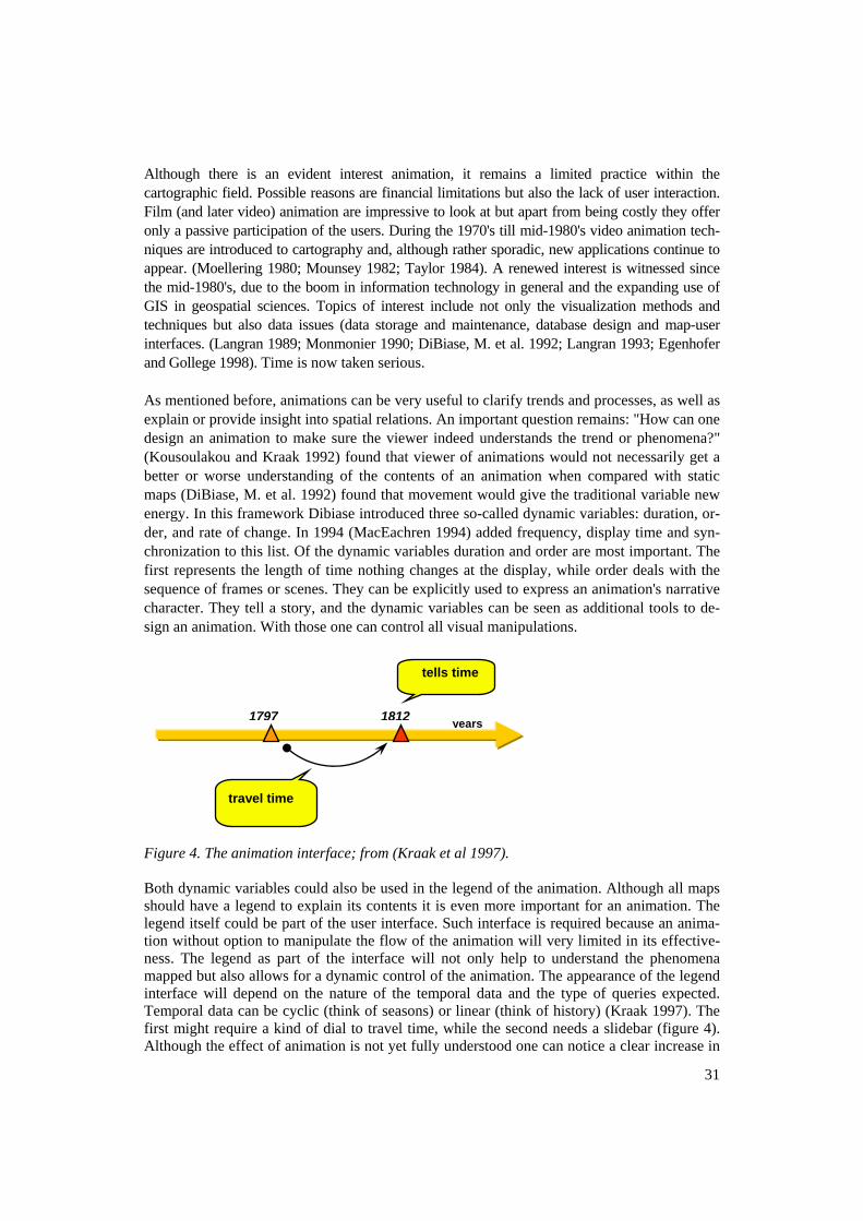
Although there is an evident interest animation, it remains a limited practice within the cartographic field. Possible reasons are financial limitations but also the lack of user interaction. Film (and later video) animation are impressive to look at but apart from being costly they offer only a passive participation of the users. During the 1970's till mid-1980's video animation tech-niques are introduced to cartography and, although rather sporadic, new applications continue to appear. (Moellering 1980; Mounsey 1982; Taylor 1984). A renewed interest is witnessed since the mid-1980's, due to the boom in information technology in general and the expanding use of GIS in geospatial sciences. Topics of interest include not only the visualization methods and techniques but also data issues (data storage and maintenance, database design and map-user interfaces. (Langran 1989; Monmonier 1990; DiBiase, M. et al. 1992; Langran 1993; Egenhofer and Gollege 1998). Time is now taken serious. As mentioned before, animations can be very useful to clarify trends and processes, as well as explain or provide insight into spatial relations. An important question remains: "How can one design an animation to make sure the viewer indeed understands the trend or phenomena?" (Kousoulakou and Kraak 1992) found that viewer of animations would not necessarily get a better or worse understanding of the contents of an animation when compared with static maps (DiBiase, M. et al. 1992) found that movement would give the traditional variable new energy. In this framework Dibiase introduced three so-called dynamic variables: duration, or-der, and rate of change. In 1994 (MacEachren 1994) added frequency, display time and syn-chronization to this list. Of the dynamic variables duration and order are most important. The first represents the length of time nothing changes at the display, while order deals with the sequence of frames or scenes. They can be explicitly used to express an animation's narrative character. They tell a story, and the dynamic variables can be seen as additional tools to de-sign an animation. With those one can control all visual manipulations.

1797 1812 years

tells time

travel time

Figure 4. The animation interface; from (Kraak et al 1997). Both dynamic variables could also be used in the legend of the animation. Although all maps should have a legend to explain its contents it is even more important for an animation. The legend itself could be part of the user interface. Such interface is required because an anima-tion without option to manipulate the flow of the animation will very limited in its effective-ness. The legend as part of the interface will not only help to understand the phenomena mapped but also allows for a dynamic control of the animation. The appearance of the legend interface will depend on the nature of the temporal data and the type of queries expected. Temporal data can be cyclic (think of seasons) or linear (think of history) (Kraak 1997). The first might require a kind of dial to travel time, while the second needs a slidebar (figure 4). Although the effect of animation is not yet fully understood one can notice a clear increase in

31

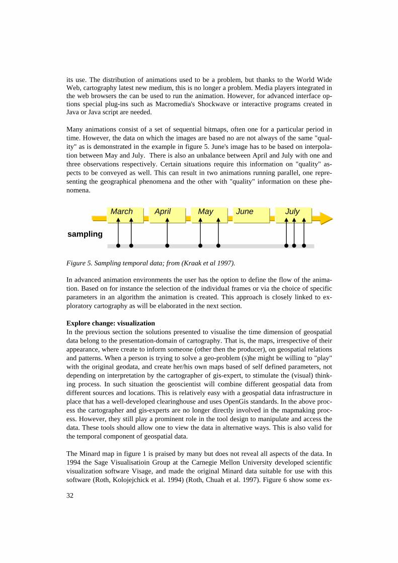
its use. The distribution of animations used to be a problem, but thanks to the World Wide Web, cartography latest new medium, this is no longer a problem. Media players integrated in the web browsers the can be used to run the animation. However, for advanced interface op-tions special plug-ins such as Macromedia's Shockwave or interactive programs created in Java or Java script are needed. Many animations consist of a set of sequential bitmaps, often one for a particular period in time. However, the data on which the images are based no are not always of the same "qual-ity" as is demonstrated in the example in figure 5. June's image has to be based on interpola-tion between May and July. There is also an unbalance between April and July with one and three observations respectively. Certain situations require this information on "quality" as-pects to be conveyed as well. This can result in two animations running parallel, one repre-senting the geographical phenomena and the other with "quality" information on these phe-nomena.

JulyJune March April

sampling

July May

Figure 5. Sampling temporal data; from (Kraak et al 1997). In advanced animation environments the user has the option to define the flow of the anima-tion. Based on for instance the selection of the individual frames or via the choice of specific parameters in an algorithm the animation is created. This approach is closely linked to ex-ploratory cartography as will be elaborated in the next section. Explore change: visualization In the previous section the solutions presented to visualise the time dimension of geospatial data belong to the presentation-domain of cartography. That is, the maps, irrespective of their appearance, where create to inform someone (other then the producer), on geospatial relations and patterns. When a person is trying to solve a geo-problem (s)he might be willing to "play" with the original geodata, and create her/his own maps based of self defined parameters, not depending on interpretation by the cartographer of gis-expert, to stimulate the (visual) think-ing process. In such situation the geoscientist will combine different geospatial data from different sources and locations. This is relatively easy with a geospatial data infrastructure in place that has a well-developed clearinghouse and uses OpenGis standards. In the above proc-ess the cartographer and gis-experts are no longer directly involved in the mapmaking proc-ess. However, they still play a prominent role in the tool design to manipulate and access the data. These tools should allow one to view the data in alternative ways. This is also valid for the temporal component of geospatial data. The Minard map in figure 1 is praised by many but does not reveal all aspects of the data. In 1994 the Sage Visualisatioin Group at the Carnegie Mellon University developed scientific visualization software Visage, and made the original Minard data suitable for use with this software (Roth, Kolojejchick et al. 1994) (Roth, Chuah et al. 1997). Figure 6 show some ex-

32

amples of the Minard-data in Visage. As can be seen in the upper map, the path the army followed has been split into segments. The segment width corresponds to the number of troops while the colour is linked to temperature. The original illustrations are in colour, where temperatures above zero are in red and below zero in blue. All original figures are interactive and linked to each other. The slide bar bellow the upper map allows one to simulate Napo-leon's march to Moscow. Moving the slide bar to the left result in the break down of the map, while a move to the right will built the map. The map show the situation on November 22, with the last bit of the retreat still missing. Next to the maps several diagrams exist. They offer a different perspective on the temporal data. The upper diagram shows the number of troops versus time. It shows that Napoleon was not constantly moving, but also remained at places for a longer time, something that Minards maps does not reveal clearly. The lower diagram shows the location of the troops in longitude versus time. Moscow is in the top mid-dle part of the diagram. Both lower map and diagram show a trajectory selected of a branch of the army going north to Pollock. Here is again becomes clear these troops stayed at Pollock for a long time before joining the retreating army. Different interactive views on the data of-ten offer fresh idea’s for a better understanding. Conclusions The visualization of geospatial's time dimension can be done according several methods. However, from a cartographic perspective these can be grouped in three categories, the single map, the series of maps and the animation. The recent application of scientific visualisation software with its interactive and dynamic characteristics offers new and alternative views on the geospatial data. This will allow researchers to explore the data, and get an even better understanding of the data compared when these would be portrayed in just one map or anima-tion. References Campbell, C S and S L Egbert 1990 Animated cartography / thirty years of scratching the surface. Cartographica 27 (2): 24-46. Cornell, B and A H Robinson 1966 Possibilities for computer animated films in cartography. The Cartographic Journal 3 (1): 79-82. DiBiase, D, M A M., et al. 1992 Animation and the role of map design in scientific visualization. Cartography and Geographic Information Systems 19 (4): 201-14. Dransch, D 1997 Computer animation in der kartographie: theorie und praxis.Springer Verlag, Berlin. Egenhofer, M J and R G Gollege, Eds. (1998). Spatial and temporal reasoning in geographic information systems. Spatial Information Systems. Oxford, Oxford University Press: Friendly, M 2000 Re-Visions of Minard. SCGN (in press) . Goedvolk, A 1988 De nieuwe relatieve afstand voor het openbaar vervoer. Nieuwe Geografenk-rant 10, 6-7. Jensen, C S and et al. 1994 A consensus glossary of temporal database concepts. SIGMOD Record 23 (1): 54-64. Kousoulakou, A and M J Kraak 1992 The spatio-temporal map and cartographic communication. Cartographic Journal 29 (2): 101-8. Kraak, M J, R. Edsall & A.M. MacEachren (1997). Cartographic animation and legends for tem-poral maps: exploration and/or interaction. 18th ICC, Stockholm: 253-61 Kraak, M J 1998 Exploratory cartography, maps as tools for discovery. ITC Journal (1): 46-54.

33

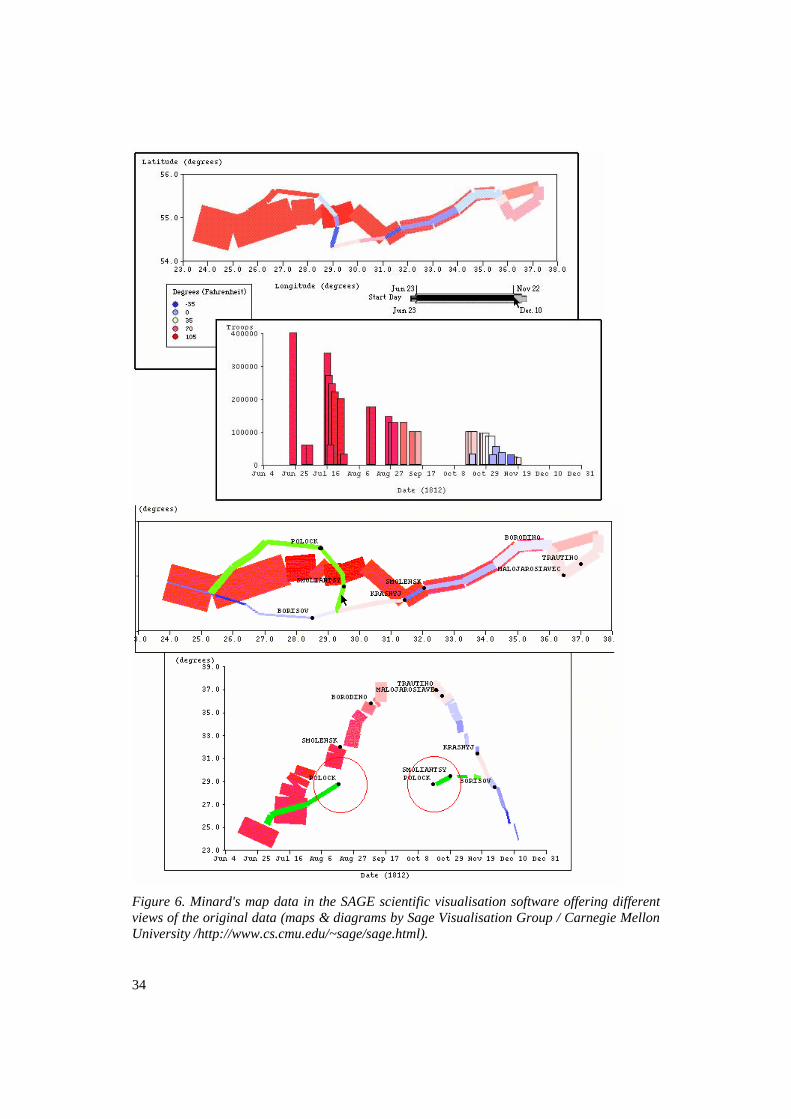
Figure 6. Minard's map data in the SAGE scientific visualisation software offering different views of the original data (maps & diagrams by Sage Visualisation Group / Carnegie Mellon University /http://www.cs.cmu.edu/~sage/sage.html).

34

Kraak, M J 1999 Dealing with time. Cartography and Geographical Information Systems 26 (2): 83-4. Kraak, M J and A M MacEachren 1999 Visualization for exploration of spatial data. International Journal of Geographical Information Sciences 13 (4): xx-xx. Langran, G 1989 A review of temporal database research and its use in GIS applications. Interna-tional Journal of Geographic Information Systems 3 (3): 215-32. Langran, G 1993 Time in Geographic Information Systems.Taylor & Francis, London. MacEachren, A, M Wachowicz, et al. 1999 Constructing knowledge from multivariate spatiotem-poral data: Integrating geographic visualization with knowledge discovery in database methods. International Journal of Geographic Information Sciences 13 (4): 311-34. MacEachren, A M 1994 How maps work: representation, visualization, and design.Guilford Press, New York. MacEachren, A M and M J Kraak 1997 Exploratory cartographic visualization: advancing the agenda. Computers & Geosciences 23 (4): 335-44. McCormick, B, T.A. DeFanti, T. A. and M.D. Brown 1987 Visualization in Scientific Computing. Computer Graphics 21 (6). Moellering, H 1980 The real-time animation of three-dimensional maps. The American Cartogra-pher 7 : 67-75. Monmonier, M 1990 Strategies for the visualization of geographic time-serie data. Cartographica 27 (1): 30-45. Mounsey, H (1982). Cartography of time-changing phenomena - the animated map. Durham, Uni-versity of Durham. Ormeling, F J (1996). Teaching animated cartography. Teaching animated cartography, Madrid, International Cartographic Association: Peterson, M P 1995 Interactive and animated cartography.Prentice Hall, Englewood Cliffs, NJ. Peuquet, D J (1999). Time in GIS and geographic databases. Geographical Information Systems: Principles, Techniques, Management, and Applications. P. Longley, M. Goodchild, D.M. Maguire and D. Rhind. New York, J. Wiley and Sons. I: 91-103. Robinson, A H 1967 The thematic maps of Charles Joseph Minard. Imago Mundi 21 : 95-108. Roth, S F, M C Chuah, et al. 1997 Towards an Information Visualization Workspace: Combining Multiple Means of Expression. Human-Computer Interaction Journal 12 (1 & 2): 131-85. Roth, S F, J Kolojejchick, et al. (1994). Interactive Graphic Design Using Automatic Presentation Knowledge. Proceedings of the Conference on Human Factors in Computing Systems (SIGCHI '94), Boston, MA,: 112-7 Snodgrass, R (1992). Temporal databases. Theory and methods of spatio-temporal reasoning in geographic space. A. U. Frank, I. Campari & U. Formentini. Berlin, Springer Verlag. 639: 22-64. Taylor, D R F (1984). Computer assisted cartography, new communications technologies and cartographic design: the need for a 'new cartography'. ICA Conference Perth, Perth: 456-67 Thrower, N 1961 Animated Cartography in the United States. International Yearbook of Cartog-raphy 1 : 20-8. Tobler, W R 1970 A computer movie: simulation of population change in the Detroit region. Eco-nomic Geography 46 (20): 234-40. Tufte, E R 1983 The visual dispaly of quantitative information.Graphics Press, Cheshie, CT. Vasiliev, I R 1997 Mapping time. Cartographica 34 (2). Wood, D 1992 The power of maps. Routledge, London.

35

Time in cadastral maps

Peter van Oosterom

Delft University of Technology,Department of Geodesy, Delft, The Netherlands

Email : oosterom@geo.tudelft.nl

Th,is po,pe:r'describes o, data rnorlel and tlte associa,tetl processes desi,gn,ed,

to rno,i,ntai,n a r:onsistertt databuse ui'th' r'espect to both topological ref-

ere.Itces o,rt,d, r:ltu'rtges ouer tirne. Tltrc nouel, contribu,ti'ons of tlt"i,s paper

are: 1. ust: of objer:t i,dentifiers cornposed of tuo Starts: oi'd, artd tinte;

2. lon,g trarr,so,t:ti,o'ns based on a r:h'eck-ou't/r:ltu:k-in rn,r:c:h,aninn,; und ,?.

start,rl,artl SQL (stru,r:tu,r'ecl c1u,er1y lan,gu,a,qe) enlt,o,rr,c:r"d uith SOL (spatial

object library) fctr both tlt,e batch product'ion' of u'pdate JiLr:s an,d for the'i,nte.rur:ti'ue u'istt,a,l,i,zation, o.f the change.s rt'uer timl:.

1 Introduct ion

Largc scale Tcipographic arr<l Cadastral clata irr tire Netherlancis [9] tr,re stored an<l

rnairrtairrcd it orr,r: integrated s'ystern based on the relational clatabase CA-Oprenlngres

with the spat ial object i ibrary (SOL) [a] and X-Firrgis [10, 11. 13]. Stor ir tg ancl

rnaintainirrg consistent topological relationships is important in a spatial clatabase.

Topology is esscntial to the nature of the Ca<lastre: parcels tnay not overlap arrdparcels should cciver thc whole territory. About 400 pcrsons (srtrveyors, ctrrtogra-

pircrs) are rrpdating these data simultancously. Aftcr the irritial delivery of all clata.

the custorners get perio<lic updates of the clatabase. Without storirrg cibject-history

iri tlrc databtrse. tlu:se u,pd,atr: fi les are rlifficult to extract [16]. Historical rlata is also

userl to {ind the previous owners of a certain polluted spot. T}ris il lustrates tlte nced

for corrsistcntly nraintaining both. tirne arrtl topology in the database.

Gcncral introduct ions to spat io-ternporal model ing are given in [1a. 18.21]t . Al-

thcirrgh scveral zr,uthors have dcscribecl a spatial-tenrporal data rnoclel arr<l query

larrguage. they ignore the problem of nraintairrirrg the clata in tlteir moclels. which is

complicate<l due to the topology references. Our data rnodcl based on topology ancl

history is preserrted in Sectiorr 2. Topological editirrg of inforrnation is discussed itt

Section 3. in which particular attention is paicl to the fact that rnr.rltiple users must

be able to work sirnultarreously. The production of update files using standard SQL(stmctured query language) is described in Section 4. In contrast tci these 'batch'

type of jobs, some possibilities for intcractive visualizatiorrs of changes over time

are given in Sectiorr 5 together with other futrue work. Finally, conclusions can be

found in Section 6.

3 6

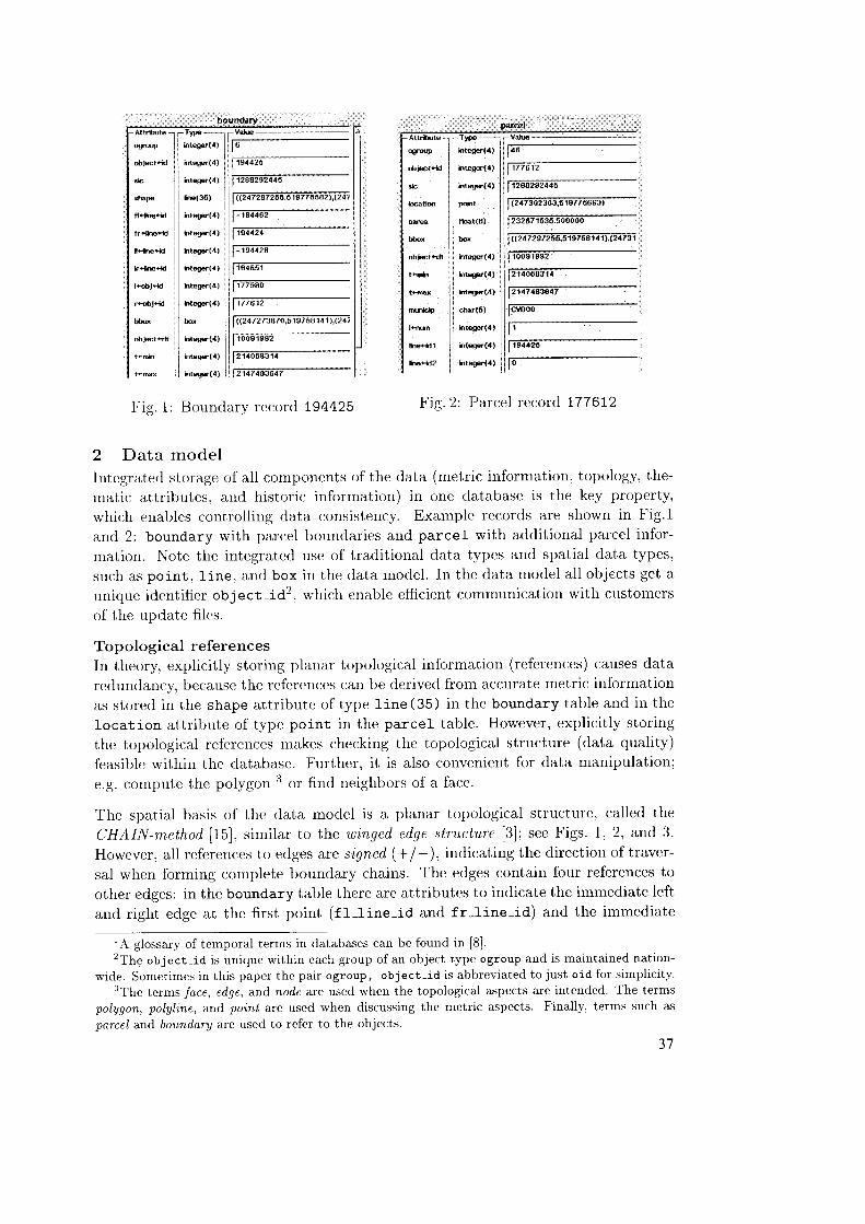
Att.b.fr

og.d.P

obj6trld

$

bcrtkn

ogdp

obirct.frt

!b

s+HP€

fllfrE.H

fr+firp.H

litE.i(l

hr{'Es

rdjd

rdi.H

bb@.

ohtsct.dt

Lt€qF(4)

htegs('tI

r(E(35)

htegd(4)

htegF(tl)

ht€qq(4)

itogd({)

iregs(4)

htegF(4)

hax

htry(4)

htggtr(6)

heg6(4)

@r@

|h

obj*tHr

tlrat

rurblp

lffi

Ef841

kE+H2

htegs{,1)

htegtr(4)

htegst4)

poett

tlda(8)

h

htogq(il)

htsgs{4)

hteg6t4t

cfnr(6)

h@d(a)

ht€gst4,

htegF(4)

F_-Frla26--

FTEEZrE4l6-Fi5;;rdtr6€3ffir;';,6w

l:ifim-

F€4iti-

Fmiz6-fE-466-1-

F7?&r-@i??7ifrdnoifr.amnfrffiErt-Fii65ftil-

| (2473O23O3,519776663'

I zs267r636,6ooooo

| ( (247297255.519768r41),{24l31

f5-dslrE-

t?fi66-Fiii'--

Ffiil656;--

lffi6d-

r-fra?5-lr--

Fig. 1: Botttrclary record 194425 F-ig.2: Parcel record 777612

2 Data model

Irrtegratecl storage of all cornponents of the clata (metric information, topology. the-

rlatic attributes. arrd historic information) in one database is the key property,

which enal)les controllirrg data consistency. Exarnple records are shown in Fig.1

and 2: boundary with parcel bourrdaries and parcel with additional parcel infor-

mation. Note the integratecl use of traditional data types and spatial data types,

such as point, line. and box in the data modcl. In the data model all obiects get a

urrique identifier object-id2. which cnable efficient cornrnunication with customers

of the update files.

Topological referencesIn theory, explicitly storing planar topological irtformation (references) causes data

rcdunclancy, because the refererrccs can be derivecl frorn accurate metric information

as stored in the shape attribute of type line(35) in the boundary table arrd in the

Iocation attribute of type point in th.e parcel table. However, explicitly storing

the topological references makes checking the topological structure (data quality)

feasiblc within the clatabasc. Frrrther, it is also convenient for data manipulation;

e.g. corr).pute the polygon r or find neighbors of a face.

The spatial basis of the data model is a planar topological structure, called the

CHAIN-method ll5], sirnilar to the w'inged edge structure l3l; see Figs. 1, 2, and 3.

However, all references to edges are signed (+l-), indicating the direction of traver-

sal when forming complete boundary chains. The edges contain four references to

other edges: in the boundary table there are attributes to indicate the immediate left

and riglrt edge at the first point (f I-1i-ne-id and fr-l-ine-id) and the immediate

1A glossaty of temporal terms in databases can be found in [8].2The object- id is unique within each group ofan object type ogroup and is maintained nation-

wide. Sometines in this paper the pair ogroup, object- id is abbreviated to just oi.d for simplici ty.3The terms t'ac.e, edge, artd node are used when the topological aspects are intended. The terms

polygon, polgli,ne, ar.d po,int are used when discussing the metric aspects. Finally, terms such as

parcel arnd boundary are used to refer to the objects.

37

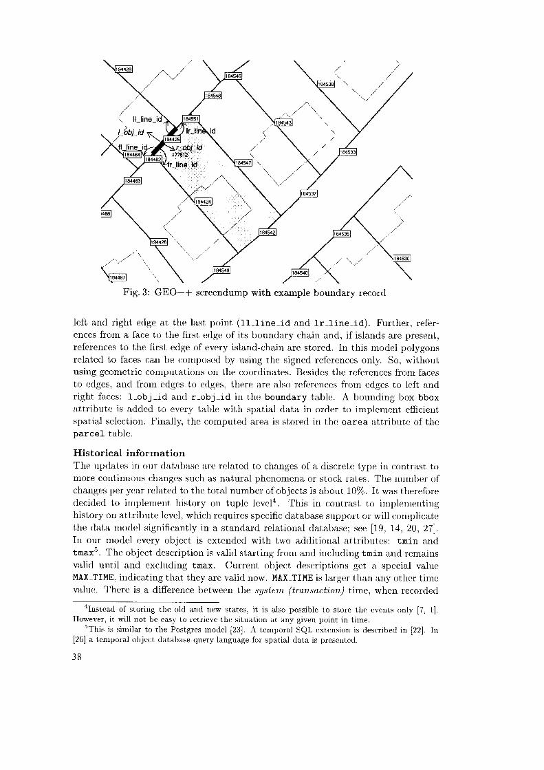
1 ll_line_id

Fig.3: GEO++ screendump with example boundary record

left and right edge at the last point (ft-tine-id and lr-line-id). Further, refer-ences from a face to the first edge of its boundary chain and, if islands are present,references to the first edge of every island-chain are stored. In this model polygonsrelated to faces can be composed by using the signed references only. So, withoutusing geometric computations on the coordinates. Besides the references from facesto edges, and from edges to edges, there are also references from edges to left andright faces: 1-obj-id ancl r-obj-id in the boundary table. A bounding box bboxattribute is added to every table with spatial data in order to implernent efficierrtspatial selection. Firrally, the computed area is stored in the oarea attributc of theparcel table.

Historical informationThe updates in our database are related to changes of a discrete type in contrast tomore continuous changes such as natural phenomena or stock rates. The nurnber ofchanges per yoar related to the total rrumber of objects is about l0o/o. It was thereforedecided to implement history on tuple levela. This in contrast to irnplementinghistory on attribute level, which requires specific database support or will complicatethe data model significantly in a standard relational database; see [19, 14, 20, 27].In our model every object is extended with two additional attributes: tmin andtmax5. The object description is valid starting from and including tmin ancl remainsvalid until and excluding tmax. Current object descriptiorrs get a special valueMAX-TIME, indicating that they are valid now. MAX-TIME is larger than any other timevalue. There is a difference between tlne system (transaction) time, when recorded

"Instead of storing the old and new states, i t is also possible to store the events only [7, 1].However, it will not be easy to retrieve the situation at anv givel point in tirne.

sThis is similar to the Postgres model [23]. A temporal SQL extension is described in [22]. In

[26] a temporal object database query language for spatial data is presented.

3 8

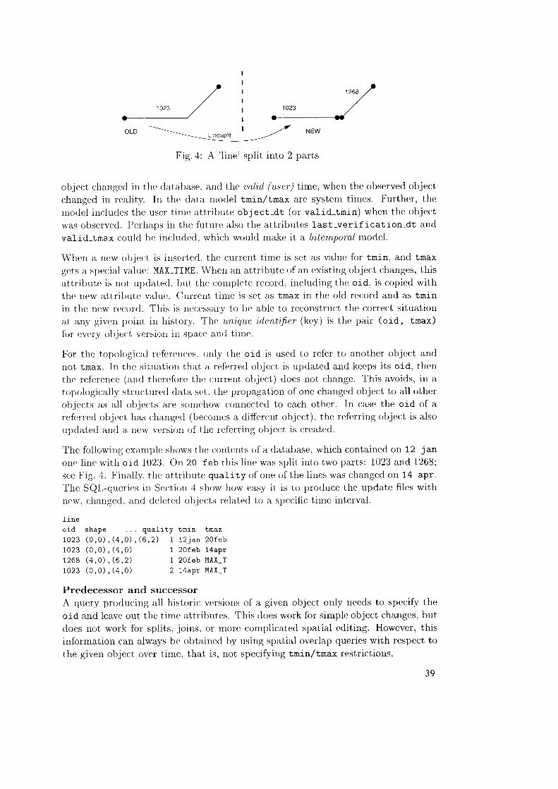
o-

OLD

Fig. 4: A ' l ine ' sp l i t in to 2 par ts

olriect changed irr. thc clatatrase, and the uo,l id, (usrt ')t irne, whert the observed object

changecl irr rcality. In the data ncidel tmin/tmax are system times. Further, the

rnor le l inc luc lcs the user t i rnc at t r ibute object-dt (or va l id- tmin) when the object

was observetcl. Pcrhaps in the futrirc also the attribrrtes Last-verif ication-dt and

valid-tmax r:oulcl be inc:lu<lccl. whicir would rnake it a bitentpctral moclel.

Wheri a ncw obje<:t is insertcd, tht-' currerrt t irnc is set as value for tmin, ancl tmax

gcts a specizrl vahrc: MAX-TIME. Whcrr an attribute of arr existing object changes, this

attri lntc is not rrltcl:rtr:rl. brrt t l ir: cornpletc rct;orcl, incluclirrg thc oid, is r:opied with

the new attri l trrtc valuc. Crrrrerrt t ime is set as tmax in the old record and as tmin

in the ncw rt:<:orrl. This is ncct:ssary to bc al:rle to reccinstrtrr:t the correct situaticin

zrt arry given poirrt irr histc.rt 'y. Tlx.- un,ir1ue, ir lenti,f ier (key) is the pair (oid, tnax)

fcir cvcly ob.jer:t versiorr irt spar:e antl t irrrc.

For the topologir:ai referenc;es. only the oid is rrsecl to refer to arrothcr object and

rrot tmax. In thr-. situatiorr that a referrerl objcct is update<l arrcl keeps its oid, then

tire rcfercncc (and therrefrrrc thc t:urrent ob.jer;t) <locs not change. This avoids, in a

topologically stnrctrrre<i data set. the propagation of one changcd object to all other

cib.jects as all ob.jc<:ts are sornchow conner:te<l to cach other. Irr r:ase the oid of a

referrerl ob.jcct has changerl (becorrrcs a ciiffererrt otrject). the referring object is also

rrpclate<l arxl a ncw versicln of the rclerring clbiect is crcatecl.

Thc followirigexanryrlt: sirciws the contcnts of a clatabase. which containe<l on 12 jan

one l i r re wi t i r o id 1023. On 20 f eb th is l ine was spl i t i t t to twr-r par ts : 1023 and 1268;

see Fig.4. F inal ly . thc at t r ibute qual i tyof or le of the l i r res was changer l on 14 apr .

The SQl-clueries irr Scction 4 show how easy it is to prorluce the update fi les with

new. charrgccl. and cleletecl ob.jccts related to a spccific t ime irrterval.

l i neo id shape . . . qua l i t y tm i -n tmax1 0 2 3 ( 0 , 0 ) , ( 4 , 0 ) , ( 6 , 2 ) 1 1 2 j a n 2 0 f e b1 0 2 3 ( 0 , 0 ) , ( 4 , 0 ) 1 2 0 f e b 1 4 a p r1 2 6 8 ( 4 , 0 ) , ( 6 , 2 ) 1 2 0 f e b M A X - r1 0 2 3 ( 0 , 0 ) , ( 4 , 0 ) 2 1 4 a p r M A X - T

Predecessor and successorA query producing all historir; versions of a given object only needs to specify the

oid and leave out the tirne attributes. This does work for sinrple object changes, but

does not work for sprlits, joins. or more conlplicated spatial editing. However, thisinforrnation can always be obtaincd by usirrg spatial overlap queries with respect to

the given obiect over tiure, that is, not specifying tmin/tmax restrictions.

39

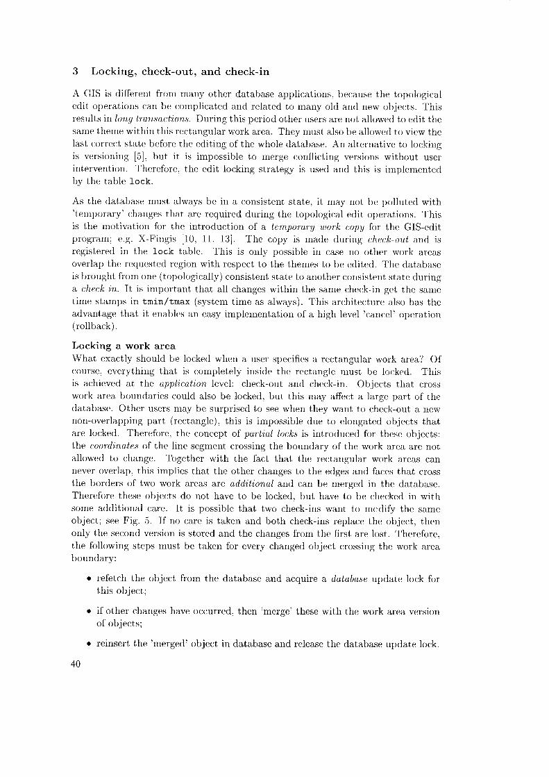
3 Locking, check-out, and check-in

A GIS is different from many other database applications, because the topoiogicaledit operations can be cornplicated and related to many old arrd new objects. Thisresults in lon11 tran,sct,ctions. Durirrg this period other users are not allowed to edit thesame therne within this rectangular work area. They nmst also be allowed to view thelast corrcct state befcrre the editing of the whole database. An alternative to lockingis versioniug 15] , but it is impossible to rnerge r;onflicting versions without userintervention. Therefore, thc edit locking strategy is used and this is irnplementeclby the table Lock.

As the database nmst always be in a consistent state, it rnay ncit be polluterl with'temporary' changes that are requirecl during the topological edit operations. Thisis the motivation for the introduction of a ternporary work copy fbr the GIS-cditprogram; e.g. X-Fingis 110, 11, 13]. The copy is made durirrg check-out an<l isregistered in the l-ock table. This is only possible in case no other work areasoverlap the requested region with respect to the themes to bc cdited. The databaseis brought from one (topologically) consistent state to arrother consistent state duriug-a chec:k-'in. It is important that all changes withirr. the same check-in get the sarnctime starrrps in tmin/tmax (svstem tirne as always). This architecture also has theadvantage that it enables an easy implernent,ation of a high level 'canccl' operation(rol lback).

Locking a work areaWhat exactly should be locked whcn :r user specifies a rectangular work area'l Ofcourse) everything that is cornpletely inside the rectangle rnust be locked. Thisis aclrieved at the upplicat'ion Ievel: check-out and check-in. Objects that c:rosswork area bounclaries could also be locked, but this nray affect a large part of the<la,tabase. Other users may be surprised to see when they want to check-out a newnon-overlappirrg part (rectangle), this is impossible due to clorr.gated objects thatare lockerl. Thereforc, the concept of partial locks is introcluced for these ob.jects:tbe coord'inates of the line segrnent crossing the bourrdary of the work area arc notallowed to change. Together with the fact that the rectangular work areas canrrever overlap, this implies that the other changes to the edges and faces that crossthe borders of two work areas are add'it ' ional and can be merged in the database.Therefore these objects do not have to be locked, but have to be checked in withsome additional care. It is possible that two check-ins want to rncdify the sanreobject; see Fig. 5. If no care is taken and both check-ins replace the ob.ject, thcnonly the second versiorr is stored and the changes frorn the first are lost. Therefore,the following steps must be taken for every changed object crossing the work areaboundary:

o refetch the object from the database and acquire a database update lock forthis object;

r if other changes have occurred, then 'merge' these with the work area versionof objects;

o reinsert the 'merged' object in database and release the database update lock.

40

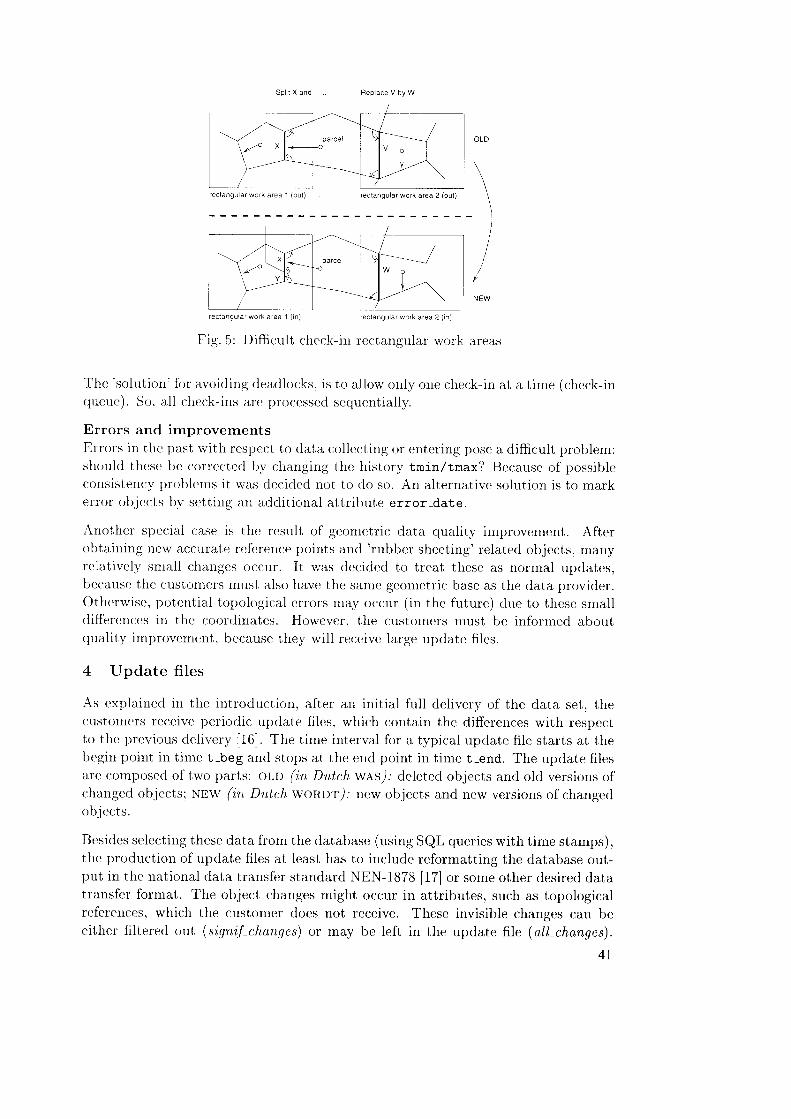
,/o xT

-o

Spl t X and

r e c l a n g u a r w o r k a r e a 1 ( o u t )

Replace V by W

rectangular work area 2 (out)

lparce

.o\ta

rectanguiar work area 1 ( in) reclangular work area 2 ( n)

Fig.5: Difficult chcck-irr rec:tangulal work

Thc 'solrrt iorr'

for avoirl ing cleardlocks. is to allciw orrly orre check-in at a tirne (cher;k-inqtrcrrer). So. all c:ireck-ins ir.rc processed sccpcntially.

Errors and improvements

Errors in thc pzrst with respect to data collccting or entering l)ose a diff icult problem:sliorrlr l thcsc bc correctc<l lty changing thc history tmin/tmax? Becausc of possibler:ortsisten<:y problerris it was decicied not to clo so. An alterrrative solution is to markerrcir obiccts by sertting an additional attrit lrte error_date.

Another spcciai c::rse is thc resrrlt of gconretric data cluality irnprovcnrcnt. Afterobtairi ing l)cw acclrrater rcfcrent:e pciints ancl 'nrblter shr:cting' related objects. ntarryrelativcly srrrall chatrgcs oc:cllr. It was <lecidecl to trcat these as norrnal upclatcs,bccatrse the custotrtcrs rriust also have the same gcorrretric basc as the data provider.Othcrwise. potential tt ipological crrols mi:Ly occur (in the futurc) due to these srnalldifferctrccs iri the coortl irrates. However. the custonrers rnust bc irrforrned aboutclrality imprcivcrricrit. becausc they wil l reccivc large updatc fi les.

4 Update f i les

As explainecl in the introductiorr. after an initial full deliverl' of thc data set, thecustotncrs receive periodic update filcs. which contain the differences with respcctto tlte previous clelivery 116]. The tirne interval {br a typical upclate file starts at theltegin point in tinre t-beg and stops at the end point in tirne t-end. The update filesare composcd of two parts: oro (in Dutch wAS): deletccl obiects and old versions ofclrangcd ob.jects; NEw (iz Dtftch woRDT/; rrew objccts arrd new vcrsions of changedob. jects.

Besides selecting these data frorrr the database (using SQL queries with time stamps),thc production of upclate files at least has to include reformatting the database out-pttt in the national data transfer standard NEN-1878 [17] or some other desired datatrarrsfer forrnat. The object changes might occur in attributes, such as topologicalrcfercnces. which the customer does not recerive. These invisible changes can beeitlrer filtered oft (signif-chanqe,s) or may be left in the update fi\e (all-changes).

4 1

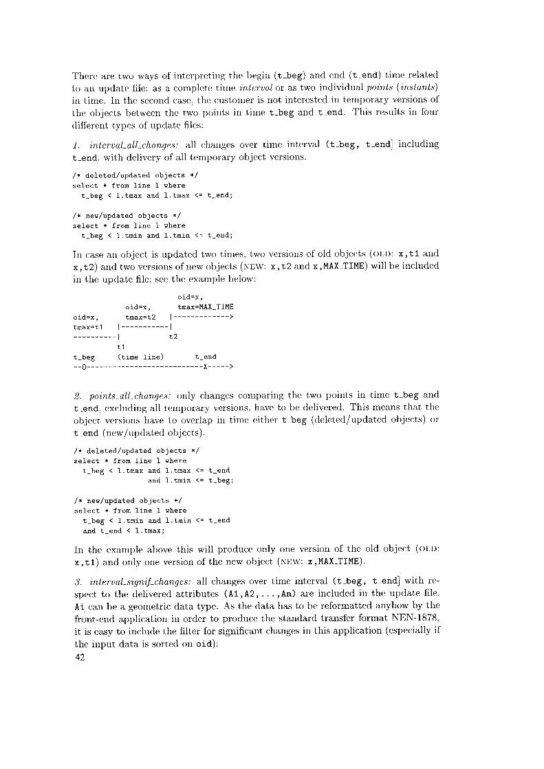
Therc are two ways of interpreting the begin (t-beg) and end (t-ena) time related

to an update file: as a complete tiure 'interuo,l or as two individual points (i,nstants)

in tirne. In the second case, thc custorrrer is not intcrested in tentporary versions of

the objects betwecn the two poirrts in tirne t-beg and t-end. Tiris results in four

different types of update files:

f . interual-all,-ch,u.nges: all changes over time interval (t-Ueg, t-end] including

t-end. with delivery of all ternporary object versions.

/ * deleted/updated objects * /

select * f rom l - ine I shere

t -beg < 1 . tmax and l . tmax <= t - end ;

/ * nes /upda ted ob jec t s + /

select * f rom l ine l - shere

t -beg < 1 . tm in and l . tm i . n <= t - end ;

In case an object is updated two times, two versions of old objects (oln: x,t1 and

x , t2) and two versions of new objects (Nnw: x , t2 and x , MAX-TIME) will be included

in the upclate file; see the example below:

o i d = x ,

tmax=t2

o i d = x ,

t rnax=MAX-TIME

o i d = x ,t m r Y = t 1 l - - - - - - - - - - - '

I t 2

t 1t -beg ( t ime l ine)- -0 - - - - - - - - - - - - - - - - x - - - - ->

2. poirtts-all-changes: only changes conrparing tl ie two points in time t-beg and

t-end, excluding all ternporary versions. havc to be delivcred. This Ineans that the

object versions have to overlap in time either t-beg (deleted/updated objects) or

t -end (new/updated objccts) .

/ * deleted/updated objects * /

se l ec t * f r om f i ne I whe re

t -beg < l . tmax and 1 . tmax (= t - end

and 1 . tm in <= t _beg ;

/ * new /upda ted ob jec t s * /

select * f rom Line 1 where

t -beg < l - . tm in and l . tm in <= t - end

and t - end ( l . tmax ;

In the example above this will produce only one version of the old object (ot o:

x, t1) and only one version of the new object (Nnw: x,MAX-TIME).

3. 'interual-s'igni,f-changes: all changes over time interval (t-beg, t-end] with re-

spect to the del ivered attr ibutes (A1 ,A2,. . . ,An) are included in the update f i le.

Ai can be a geometric data type. As the data has to be reformatted anyhow by the

front-end application in order to produce the standard transfer format NEN-1878,

it is easy to include the filter for significant changes in this application (especially if

the input data is sorted on oid):

t _end

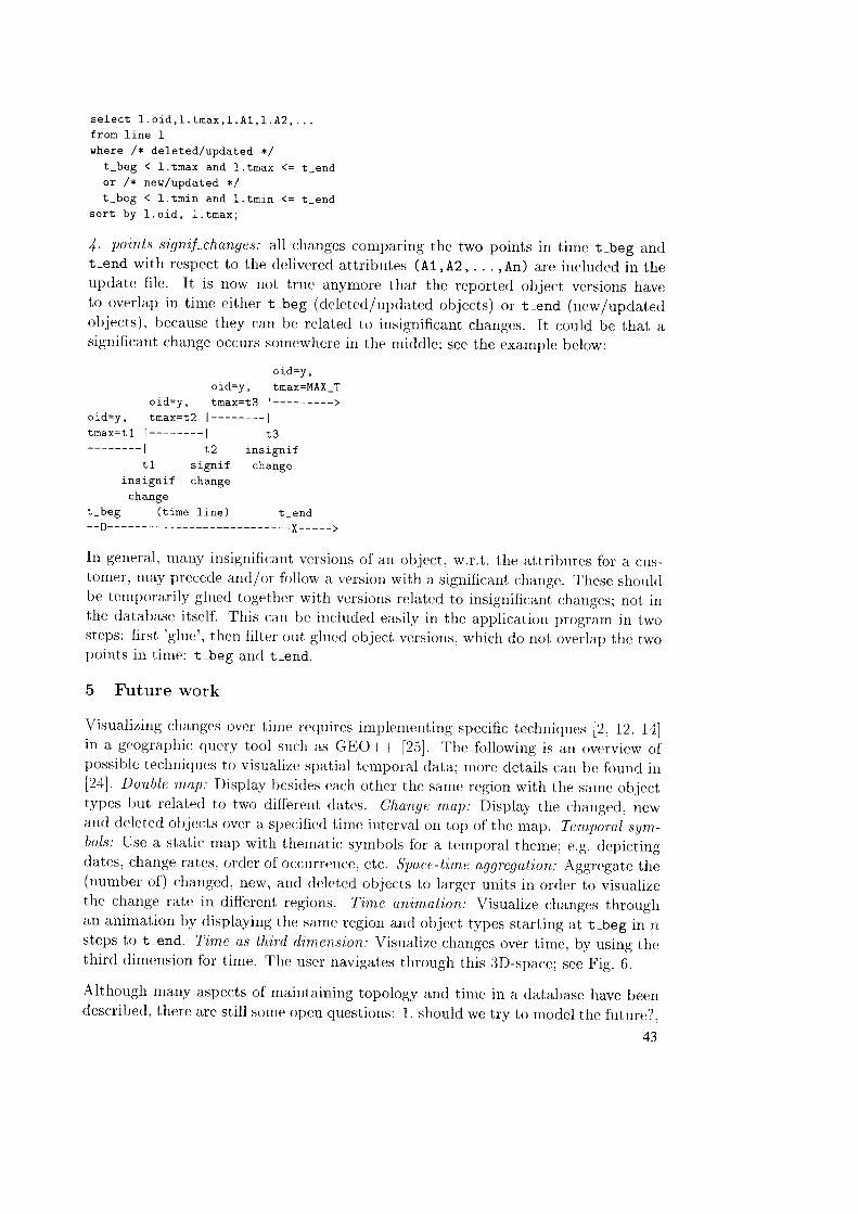
s e l e c t I . o i d , 1 . t m a x , 1 . A 1 , 1 . A 2 , . . .f rom l ine I

vhere /+ deleted/updated * /

t - beg < 1 . tmax and l - . tmax <= t _endor /* la" lopdated * /

t - beg < l . t n i n and l . tm in <= t _ends o r t b y 1 . o i d , l . t m a x ;

y'' points-siqn'if-chan,ges.' all changes comparing the two points in time t-beg an4t -end w i th respcc t to the dc l i vercd a t t r ibu tes (A1,A2, . . . ,An) a re inc ludec l in theupdate file. It is now not true anynrore that the reported object versions haveto overlap in titrte eith.er t-beg (deleted/updated objects) or t-end. (new/updateclobjects). because they can be related to irrsignificant changcs. It colld be t|at asignificant changc occurs sorncwhere in the middle; see the example below:

o i . d=y ,

o i d=y , tmax=MAX_T

o id=y , tmax= t3 | _________>

o i d = y , t m a x = t 2 | - - - - - - - - Itmax= t1 I - - - - - - - - | t 3- - - - - - - - l t ) i r c i a n i f

t 1 s i gn i f change

insigni f change

change

t -beg ( t ime f i ne ) t _end- -0 - - - - - - - - - - - - - - - -X - - - - ->

In general. malry insignificarrt vcrsions of an objerct. w.r.t. the attribrrtcs fclr a cus-tcinter, rl lay preccde and/or folkrw a versiorr with a significant changc. T|cse shoulclt le tcrrtporarily glrrecl togethcr witir versiorrs relatecl to insigrrif icant challgcs; not irrthe database itself. This r:arr bc irrclucled easily in the applicatiorr pro€garn irr twosteps: f irst 'gluet', then fi l ter orrt glued object vcrsions. which <io not overlap the twcrpoints in t i rne: t_beg arr r l t_end.

5 Future work

Visualizing changes over tirrre reqrrires irnprlenrentirlg specific techrriquc's l2. 12, 14)in a geographic querv tciol such as GEO++ [25]. The fcrllowing is arr overview ofpossible techniqttes to visualizc spatial temporal data: more details can be lbund inl2a]. Double nlop: Display besirles cach cither thc samc refiion wit]r the sarne obiecttypes lrrrt relatecl to two clifferent clatcs. Chan,ge rnap: l)isplay tlie cirangefl. 1ewand deletecl objects over a specific<l timc interval on top oJ'the rnayt. Tr:rn,ytorul s,grl-bol.s; Use a statir: ntap with thernatic symbols for a ternporal thenre; e.g. depictilgclates' clrange rates. orcler o1'occttrrence. etc. Space-tim,e u,qgreqo,tion: Aggregate the(tluurber rtf) changed, llew, and dcleted objects to larger units in order to visualizcthe charrgc ratc in different regions. Ti,m,e animation: Visualize changes throughan aniuration by displaying the sarne region and object types starting at t_beg in 2steps to t-end. T'irn,e as third dime'nsion: Visualize charrges over tirne, by using thethircl dirnension for time. The user navigates through this 3D-space; see Fig. 6.

Although nralty aspccts of rnaintaining topology and tinre in a database have beelclesr:ribed, there are stil l sonre open questions: 1. should we try to rnodel the flture?,

43

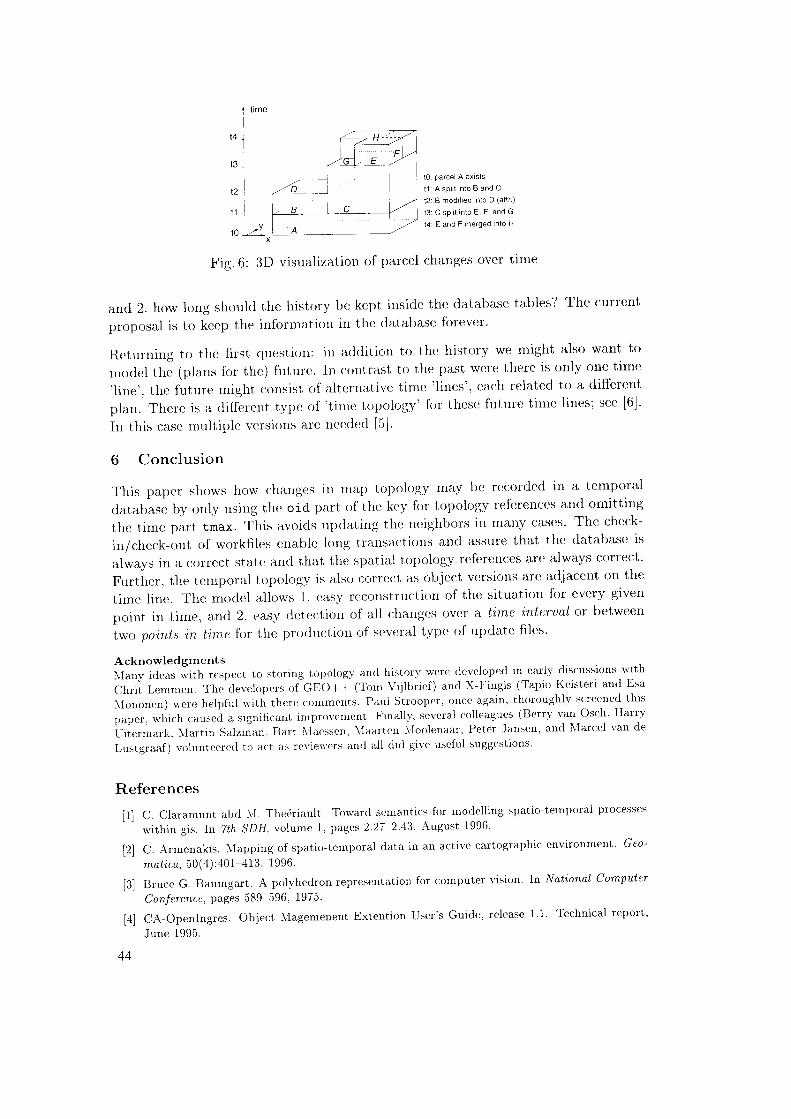
i rme

t 4 ,

t ?

t l l

n l.-YX

t0: parcel A exlsts

t1 : A sp l i t in to B and C

t2: B modified into D (attr.)

t3: C split into E, F, and G

t4: E and F merged into H

Fig.6: 3D visual izat iotr of I )arcol changes over t ime

a.cl 2. how long shoulrl thc history bc kept inside the <iatabasc tables? The r;urrent

ltroposal is to kecp the infortnzrti<tn in thc clatabase fbrever.

R,cttrrning to thc first rlresticlrr: irr arlclition to thc history we nright also want to

model the (pltrrrs for thc) futrrre. Itr r:orltrast to the past wcre therc is ottly one time'line'. the futrtre nright consist cif alternative tinrc 'l inr:s', car:h relatcd to a difl 'erent

pla'. TSerc is a cliffercnt typc of 'tirne to1;ology'fbr thesr: futtrre tirnc lines; see [6]'

In this case multipic versions are neederd [5]'

6 Conclusion

This paltcr shows how changes irr rnall tollologV may bt: rccorde<l in a tcmporal

clatabasc by orrly usirrg thc oid part of thc kcy for topokrgy refcrences ancl ornitting

the tirrtc part tmax. This avoicls rrp<latirig the ncighll<-rrs irr many r:ases' The cher:k-

i'/check-orrt cif workfilcs cnable lorrg transactic-urs anrl assttre that thc datallast' is

always in a corrcct statc arrd that the sp:r,tial topology re{'erences are alwaYs correct'

Furtltcr. the terrr.ltoral topology is alst,i corre<;t ns object versions are adjacent orr' the

ti're line. Tirc rrioclel allows l. casy reconstnrr:tiorr of the situation for cvery grven

poirrt in time. arr<l 2. easy <lctectiti lr of all r:hanges ovel a ti 'rne inter"ual or betweerr

twct po,ints ,in tim,r: fcir thet produr:ticlrr Of scveral typrr: clf tllltlate filcs.

Acknowledgments

\{a.v iclels rvit}r rt:spet:t to storing top(}log}' ancl historv rvcre tlevcloptld in early <Iiscussions rvith

chr i t Lcrnmen. The c levt : lopers u icE<l++ (Torn Vi . j lbr ief ) and X-Fir rg is (Tapio Keister i ancl Esa

\ Io 'one1) tverc hglpfu l t i , i th therc col l lmcl l ts . Paul Strooper i oI ICe again, thoroughlv s<lrcened th is

p,aper. .rvirir:h c:rusecl a significarrt irrrprovement. Finally, sevtlral colleagtrcs (Bcrry van osr:h, Harrv

Ui t r : r rnark. \ Iar t in Salzrnan. Bart \ iaesscn, \ laarten \ loolenaar, Peter .Jansen, and \ ' {arcel van de

Lustgraaf) voluntcere<l to act as rr tv ie\ \ ,crs and i r l l d i< i g ive uscful suggt 's t iorrs

References

[1] C. Claramunt abcl NI. The6riault . Tos.ard serrrantics for moclel l ing spatio-ternporal processes

*' i thin gis. In 7lh ,5D11, volumc 1. pages 2 27 213, August 1996

[2] c. Armenakis. ] , Iapping of spatio-temporal data in an active cartographic environrnent Geo-

m,a t ica . 50( '1 ) : '101 413, 1996.

[3] Bruce G. Baurngart. A pol i ,heclron representation for colnputer vision. In Nat' ional Computer

Conference, Pages 589 596, 1975.

l ] CA-Openlngrcs. Object \ , Iagemenent Extenti0n User's Guidc, release 1' l Technical report '

June 1995.

44

[5] \ I . E. Easterf ield, R. Ci. Nervcl l , andD. G. Theriault . \ 'ersion managerncnt ir t gis appl icat ious

and techniclues. In -EG1^9'90. pages 288 297, Apri l 1990.

[6] A. U. Frank. Qualitative tcrrrporal rcasorring irr GIS ordered time sr:ales. In 6th SDH, ltages,110 130, September 199,1.

[7] C. \1. Golcl. An cverrt-cLiven:rpproac:h to spatio-tclnpor:r l m:rppirrg. Geornnti tu, 50(4): l1j 42'1,

1996.

[8] C. S. . Iensen, J. Cl i f ford. irnd R.. Elrnasri . A r:onscnsus glt issarv of tenrporal <latab:rsc corrcepts.

S IGM( )D Rrcord . 23( t ) :6 i 86 . I99 '1 .

[9] Kadaster, Direct ie Gcodesie. Handboek LKI - extern. technischc aspecten. Technical roport,

Dienst van het Kadaster en dc Openbarc R.egistcrs, Novembcr 1989. (In Dutch).

[10] Karttakeskus, Helsinki, Finland. Firrgis User \ lanual, r 'crsion 3.85. Technical rcport, 199'1.

[11] T. Keistcri . Fingis softrvare and data rnanipulat ion. Tn Au"to Carto Lo'n'don volume 1, pagcs

69 75, Septernber 1986.

[12] \ I . J. Kraak ancl A. NL NIacEat:hrcrr. \ , ' isual izat ion of the ternporal cornponont erf spatial clata.

h 6th SDH, pages 391 409, Septcrnber 199'1.

113] KT-Datacenter Ltd., Ri ihimiiki , Finlancl. X-Fingis Softrvare \ '1.1, INGRES vcrsion. Tcchrrical

repor t , Oc tober 1994.

[11] G. Langran. T, irne. in Geographic Information Systerns. Taylor & Francis, London, 1992.

[15] C. Lemmcn arrd P. van Oosterom. Eff icient and automatic procluct iou of periocl ic upclatcs of

cadastral rnaps. In JEC-GI'95, pages 137 1'12, Nlart:h 1995.

[16] C. H. J. Lemmen and B. Keizt:r. Levering varr rnutat ies uit de LKl-Eiegevcnsbarrk. Geod'e siLt,

35(6) :265 269. September 1993. ( In Dut<rh) .

I i7] NEN-1878. Automatisc]re gegcvensverrvcrkirrg - Uit lvissel ingsforrnaat voor gegevens over

cle aan het aardoppervl:rk gcrelateercle mimtel i jke obje<:ten. Technical report, Neclerlancls

Normal isa t ie - ins t i tuu t . , lun i 1993. ( In Dutc i r ) .

[18] D. Pr:uquet ancl L. () ian. An irrtegratcrl datab:isc design for tcrrrpor:r l gis. I t Proceedirtgs

of tlle 7th Inte.rn,ational Syrnposiu.rn on Spatial Data Handl'tng, Delft, Tlt'e. NetherlazrJs, pagcs

2. I 2 .11 . August 1996.

[19] D. J. Peuquet anci E. Wentz. An approac]r for t imc-baseci analvsis of spatio-ternporal data. In

6th SDH, pages 489 504, September 199'1.

[20] H. Raafat, Z. Yang, and D. Gauthier. R.elat ional spatial topologies for ]r istorir :al geographit:al

inforrnation. IJGIS, 8(2):163 173, 1994.

[21] . \ . A. Roshanrrejacl. The Managernent of Spatio-Tenrporal Do,ta in a National Geographic

Inforrnation Systern. PhD thesis, Enscherie. Thc Neth, 'r lands, Trventc Univerist-"". 1996.

f22] R. T. Snodgrass, I . Ahn, ancl G. Ari i iv. Tsc1l2 language specif icat ion. SIGMOD Recctrd,

2 3 ( 1 ) : 6 5 8 6 , 1 9 9 4 .

[23 ] NI . S toncbraker : rndL. A . Rorve . T ] redes ignof Pos tgrcs . ACM SIGMOD, 15(2) :3a0 355. 1986.

124] P. van Oosterorrr and B. \,laessen. Geograpiric qucry tool. In Third Joint European Conference

€j Erhibi,tion on Ge,ograph'ical Inforrnat'ion (JEC-GI'97), pages 177 186, April 1997.

[25] T. Vi j lbr ief andP. varr Oosterom. The GEO}] system: Anextcnsible GIS. In 5th SDH,pages

40 50, August 1992.

[26] A. Voigtmann, L. Becker, and K. H. Hinrichs. Temporal extcnsions for an object-oriented

geo-data-nrodel. In 7th,SDII, volume 2, pages 11A.25 11A 41, August 1996.

[27] N{. F. Worboys. Unifying the spatiai and temporal components of geographical inforrnatiorr.

ln 6th SDH, pages 505-517, September 199'1.

45

Hodochronologics: History and time in the National Road Database L. Heres Ministry of Transport, Public Works and Water Management Directorate-General of Rijkswaterstaat Transport Research Centre (AVV) Tel. 0031 45 5605 279 Fax 0031 45 5605 224 E-mail: l.heres@avv.rws.minvenw.nl Abstract Rijkwaterstaat’s Transport Research Centre (AVV) records detailed information about traffic and transport. This concerns amongst others: traffic accidents, traffic intensity, congestion and goods and passenger transport figures. This information is stored in a number of data-bases which all use the National Road Database (NWB) as their common reference frame. This information is used for trend analysis, predictions and policy. The time dimension there-fore plays a crucial role, both in the thematic data and the road database. That is why AVV pays much attention to the time component. The core object in the NWB Road Database is the Road Element. The time component is introduced in the conceptual data model by splitting a Road Element into a number of Road Element Ephemera’s - one for each day that the Road Element exists. Attributes and relations that may change are “attached” to the Ephemera. In the logical model Ephemera’s with identical attributes and relations are concatenated into Road Element Periods. This leads to a an additional start and end-date attribute in the corre-sponding relational table. What is stored in practice is registration time, i.e. the time that a change is recorded in the database. Theoretically, a distinction should be made between registration time and occur-rence time, i.e. the time that an object really changes. This would lead to two different time dimensions in the database. However, for pragmatic reasons, only one time dimension (registration time) has been im-plemented. Occurrence time is mostly not well known and often not sharply defined, and in 99% of the cases would be identical to registration time. Sometimes this may lead to data inconsistency. However, this is so incidental that it is not worth implementing a second time dimension. At the technical level, the table of Road Element Periods is split into two tables: one contain-ing the currently valid records, the other the outdated records. This has to do with the limita-tions of former versions of the Spatial Data Engine (SDE). The current version of SDE does not have this problem, so that in the next release of the NWB Road Database, these tables will be combined into one single table.

46

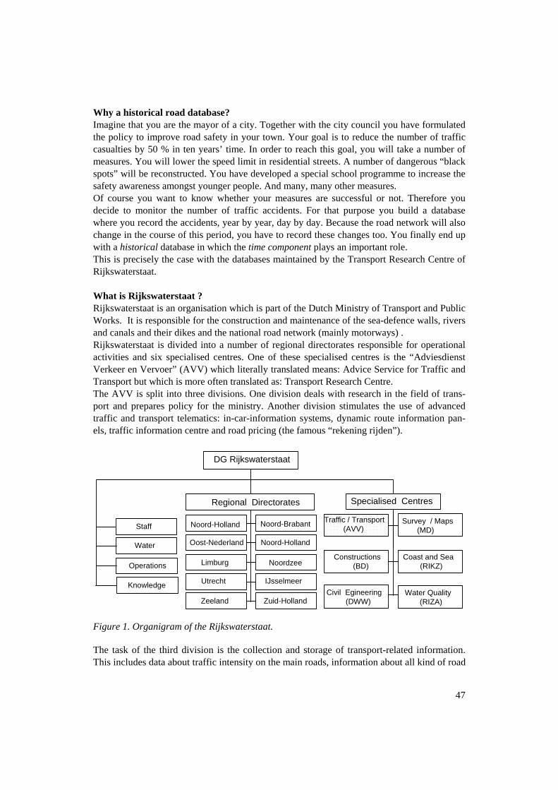
Why a historical road database? Imagine that you are the mayor of a city. Together with the city council you have formulated the policy to improve road safety in your town. Your goal is to reduce the number of traffic casualties by 50 % in ten years’ time. In order to reach this goal, you will take a number of measures. You will lower the speed limit in residential streets. A number of dangerous “black spots” will be reconstructed. You have developed a special school programme to increase the safety awareness amongst younger people. And many, many other measures. Of course you want to know whether your measures are successful or not. Therefore you decide to monitor the number of traffic accidents. For that purpose you build a database where you record the accidents, year by year, day by day. Because the road network will also change in the course of this period, you have to record these changes too. You finally end up with a historical database in which the time component plays an important role. This is precisely the case with the databases maintained by the Transport Research Centre of Rijkswaterstaat. What is Rijkswaterstaat ? Rijkswaterstaat is an organisation which is part of the Dutch Ministry of Transport and Public Works. It is responsible for the construction and maintenance of the sea-defence walls, rivers and canals and their dikes and the national road network (mainly motorways) . Rijkswaterstaat is divided into a number of regional directorates responsible for operational activities and six specialised centres. One of these specialised centres is the “Adviesdienst Verkeer en Vervoer” (AVV) which literally translated means: Advice Service for Traffic and Transport but which is more often translated as: Transport Research Centre. The AVV is split into three divisions. One division deals with research in the field of trans-port and prepares policy for the ministry. Another division stimulates the use of advanced traffic and transport telematics: in-car-information systems, dynamic route information pan-els, traffic information centre and road pricing (the famous “rekening rijden”).

DG Rijkswaterstaat

Civil Egineering (DWW)

Survey / Maps (MD)

Constructions (BD)

Coast and Sea (RIKZ)

Water Quality (RIZA)

Specialised Centres

Noord-Holland Noord-Brabant

Oost-Nederland Noord-Holland

Limburg Noordzee

Utrecht IJsselmeer

Zeeland Zuid-Holland

Regional Directorates

Staff

Water

Operations

Knowledge

Traffic / Transport (AVV)

Figure 1. Organigram of the Rijkswaterstaat. The task of the third division is the collection and storage of transport-related information. This includes data about traffic intensity on the main roads, information about all kind of road

47

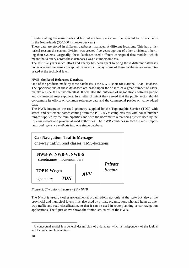
furniture along the main roads and last but not least data about the reported traffic accidents in the Netherlands (350.000 instances per year) . These data are stored in different databases, managed at different locations. This has a his-torical reason: the current division was created five years ago out of other divisions, inherit-ing their systems. Originally, these databases used different conceptual data models1, which meant that a query across these databases was a cumbersome task. The last five years much effort and energy has been spent to bring those different databases under one and the same conceptual framework. Today, some of these databases are even inte-grated at the technical level. NWB, the Road Reference Database One of the products made by these databases is the NWB, short for National Road Database. The specifications of these databases are based upon the wishes of a great number of users, mainly outside the Rijkswaterstaat. It was also the outcome of negotiations between public and commercial map suppliers. In a letter of intent they agreed that the public sector should concentrate its efforts on common reference data and the commercial parties on value added data. The NWB integrates the road geometry supplied by the Topographic Service (TDN) with street- and settlement names coming from the PTT. AVV completes this with house number ranges supplied by the municipalities and with the hectometre referencing system used by the Rijkswaterstaat and provincial road authorities. The NWB combines in fact the most impor-tant road reference methods into one single database.

TOP10-Wegen

geometry TDN

NWB-W, NWB-V, NWB-Sstreetnames, housenumbers

AVV

Car Navigation, Traffic Messagesone-way traffic, road classes, TMC-locations

PrivateSector

Figure 2. The onion-structure of the NWB. The NWB is used by other governmental organisations not only at the state but also at the provincial and municipal levels. It is also used by private organisations who add items as one-way traffic and road classification, so that it can be used in route planning or car navigation applications. The figure above shows the “onion-structure” of the NWB. 1 A conceptual model is a general design plan of a database which is independent of the logical and technical implementation.

48

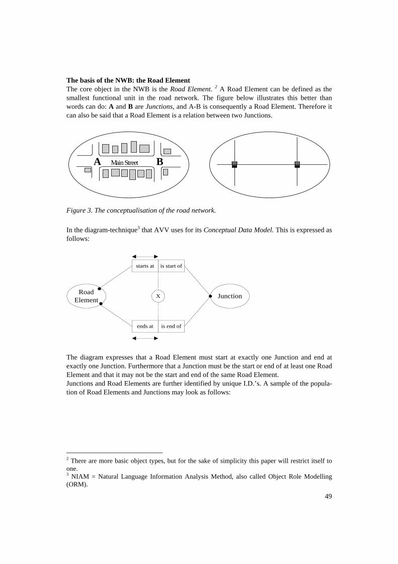
The basis of the NWB: the Road Element The core object in the NWB is the Road Element. 2 A Road Element can be defined as the smallest functional unit in the road network. The figure below illustrates this better than words can do: A and B are Junctions, and A-B is consequently a Road Element. Therefore it can also be said that a Road Element is a relation between two Junctions.

Main StreetA B

Figure 3. The conceptualisation of the road network. In the diagram-technique3 that AVV uses for its Conceptual Data Model. This is expressed as follows:

RoadElement Junction

starts at is start of

ends at is end of

X

The diagram expresses that a Road Element must start at exactly one Junction and end at exactly one Junction. Furthermore that a Junction must be the start or end of at least one Road Element and that it may not be the start and end of the same Road Element. Junctions and Road Elements are further identified by unique I.D.’s. A sample of the popula-tion of Road Elements and Junctions may look as follows:

2 There are more basic object types, but for the sake of simplicity this paper will restrict itself to one. 3 NIAM = Natural Language Information Analysis Method, also called Object Role Modelling (ORM).

49

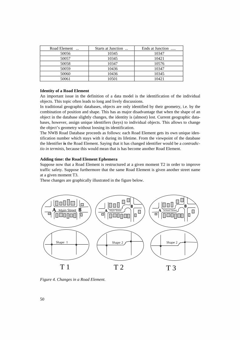
Road Element ... Starts at Junction ... Ends at Junction ..... 50056 10345 10347 50057 10345 10421 50058 10347 10576 50059 10436 10347 50060 10436 10345 50061 10501 10421

Identity of a Road Element An important issue in the definition of a data model is the identification of the individual objects. This topic often leads to long and lively discussions. In traditional geographic databases, objects are only identified by their geometry, i.e. by the combination of position and shape. This has as major disadvantage that when the shape of an object in the database slightly changes, the identity is (almost) lost. Current geographic data-bases, however, assign unique identifiers (keys) to individual objects. This allows to change the object’s geometry without loosing its identification. The NWB Road Database proceeds as follows: each Road Element gets its own unique iden-tification number which stays with it during its lifetime. From the viewpoint of the database the Identifier is the Road Element. Saying that it has changed identifier would be a contradic-tio in terminis, because this would mean that is has become another Road Element. Adding time: the Road Element Ephemera Suppose now that a Road Element is restructured at a given moment T2 in order to improve traffic safety. Suppose furthermore that the same Road Element is given another street name at a given moment T3. These changes are graphically illustrated in the figure below.

Main StreetA B Main StreetAB

School StreetAB

Shape 1

T 1 T 2 T 3

Shape 2 Shape 2

Figure 4. Changes in a Road Element.

50

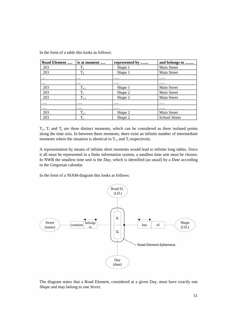
In the form of a table this looks as follows:

Road Element ..... is at moment ..... represented by ........ and belongs to ......... 203 T1 Shape 1 Main Street 203 T2 Shape 1 Main Street ... ... ..... ...... ... ... ..... ...... 203 Ti-1 Shape 1 Main Street 203 Ti Shape 2 Main Street 203 Ti+1 Shape 2 Main Street ..... ..... ..... ..... ..... ..... ..... ...... 203 Tj-1 Shape 2 Main Street 203 Tj Shape 2 School Street

T1, Ti and Tj are three distinct moments, which can be considered as three isolated points along the time axis. In between these moments, there exist an infinite number of intermediate moments where the situation is identical to T1, and Ti respectively. A representation by means of infinite short moments would lead to infinite long tables. Since it all must be represented in a finite information system, a smallest time unit must be chosen. In NWB the smallest time unit is the Day, which is identified (as usual) by a Date according to the Gregorian calendar. In the form of a NIAM-diagram this looks as follows:

Road El. (I.D.)

Day(date)

atof

Street(name)

Shape(I.D.)contains belongs

to has of

Road Element Ephemera

The diagram states that a Road Element, considered at a given Day, must have exactly one Shape and may belong to one Street.

51

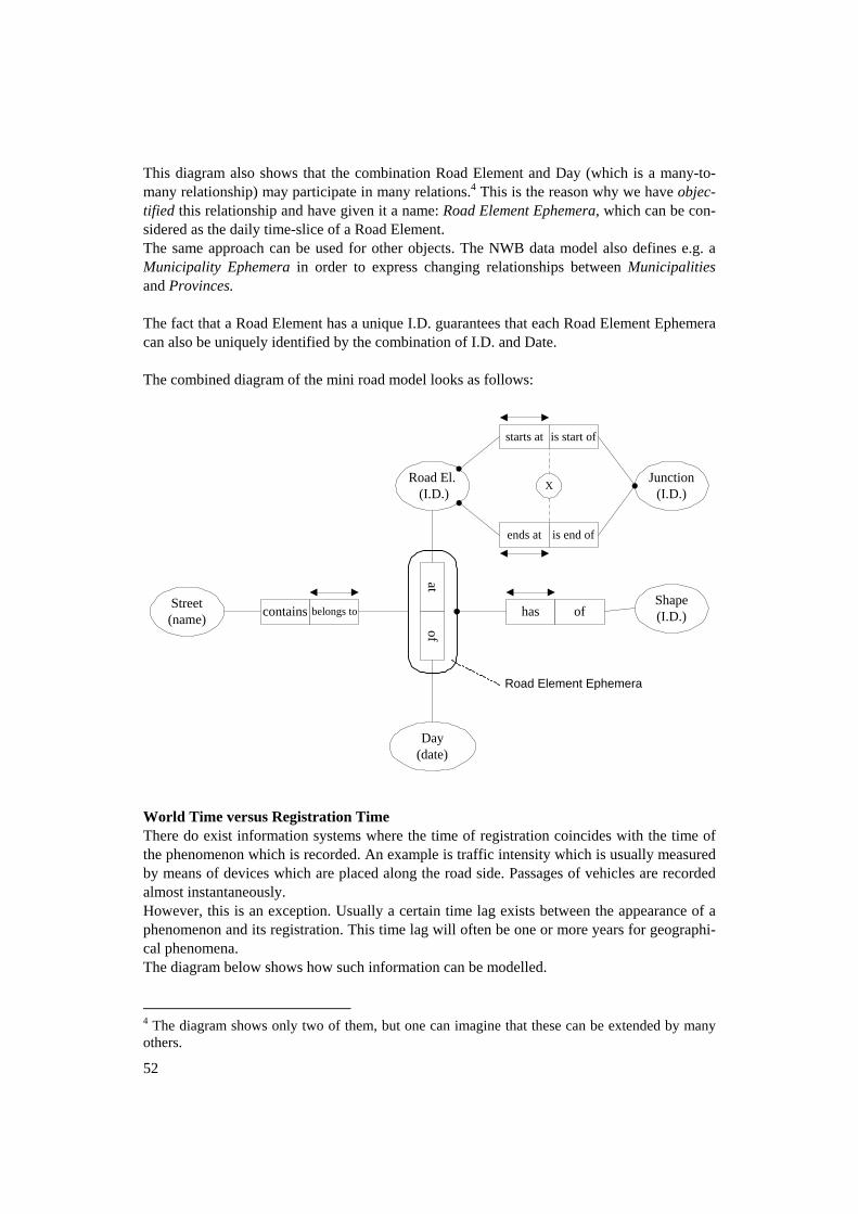
This diagram also shows that the combination Road Element and Day (which is a many-to-many relationship) may participate in many relations.4 This is the reason why we have objec-tified this relationship and have given it a name: Road Element Ephemera, which can be con-sidered as the daily time-slice of a Road Element. The same approach can be used for other objects. The NWB data model also defines e.g. a Municipality Ephemera in order to express changing relationships between Municipalities and Provinces. The fact that a Road Element has a unique I.D. guarantees that each Road Element Ephemera can also be uniquely identified by the combination of I.D. and Date. The combined diagram of the mini road model looks as follows:

Junction(I.D.)

starts at is start of

ends at is end of

XRoad El.

(I.D.)

Day(date)

atof

Street(name)

Shape(I.D.)contains belongs to has of

Road Element Ephemera

World Time versus Registration Time There do exist information systems where the time of registration coincides with the time of the phenomenon which is recorded. An example is traffic intensity which is usually measured by means of devices which are placed along the road side. Passages of vehicles are recorded almost instantaneously. However, this is an exception. Usually a certain time lag exists between the appearance of a phenomenon and its registration. This time lag will often be one or more years for geographi-cal phenomena. The diagram below shows how such information can be modelled.

4 The diagram shows only two of them, but one can imagine that these can be extended by many others.

52

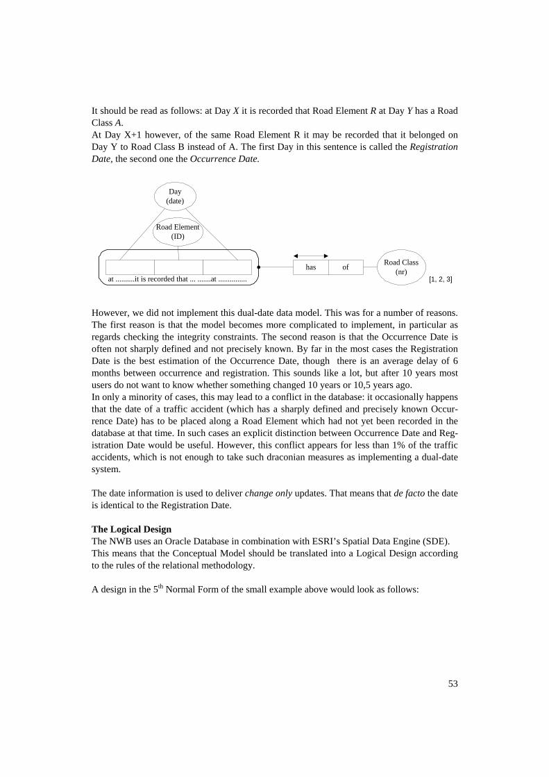
It should be read as follows: at Day X it is recorded that Road Element R at Day Y has a Road Class A. At Day X+1 however, of the same Road Element R it may be recorded that it belonged on Day Y to Road Class B instead of A. The first Day in this sentence is called the Registration Date, the second one the Occurrence Date.

Road Element(ID)

Day(date)

at ..........it is recorded that ... .......at ............... [1, 2, 3]

Road Class(nr)has of

However, we did not implement this dual-date data model. This was for a number of reasons. The first reason is that the model becomes more complicated to implement, in particular as regards checking the integrity constraints. The second reason is that the Occurrence Date is often not sharply defined and not precisely known. By far in the most cases the Registration Date is the best estimation of the Occurrence Date, though there is an average delay of 6 months between occurrence and registration. This sounds like a lot, but after 10 years most users do not want to know whether something changed 10 years or 10,5 years ago. In only a minority of cases, this may lead to a conflict in the database: it occasionally happens that the date of a traffic accident (which has a sharply defined and precisely known Occur-rence Date) has to be placed along a Road Element which had not yet been recorded in the database at that time. In such cases an explicit distinction between Occurrence Date and Reg-istration Date would be useful. However, this conflict appears for less than 1% of the traffic accidents, which is not enough to take such draconian measures as implementing a dual-date system. The date information is used to deliver change only updates. That means that de facto the date is identical to the Registration Date. The Logical Design The NWB uses an Oracle Database in combination with ESRI’s Spatial Data Engine (SDE). This means that the Conceptual Model should be translated into a Logical Design according to the rules of the relational methodology. A design in the 5th Normal Form of the small example above would look as follows:

53

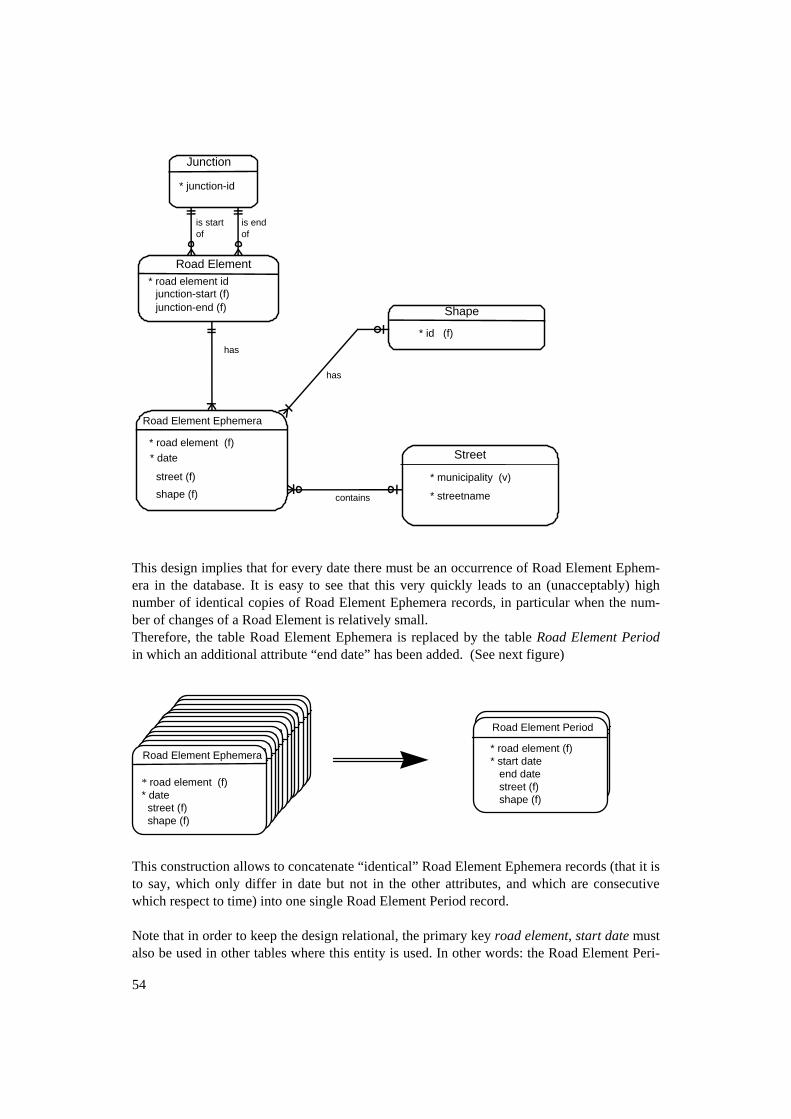
Road Element Ephemera

* road element (f)* date

shape (f)street (f)

Junction

* junction-id

is startof

is endof

Road Element* road element id junction-start (f) junction-end (f)

Street

* municipality (v)

* streetname

Shape

* id (f)

contains

has

has

This design implies that for every date there must be an occurrence of Road Element Ephem-era in the database. It is easy to see that this very quickly leads to an (unacceptably) high number of identical copies of Road Element Ephemera records, in particular when the num-ber of changes of a Road Element is relatively small. Therefore, the table Road Element Ephemera is replaced by the table Road Element Period in which an additional attribute “end date” has been added. (See next figure)

Road Element EphemeraRoad Element EphemeraRoad Element EphemeraRoad Element EphemeraRoad Element EphemeraRoad Element EphemeraRoad Element EphemeraRoad Element EphemeraRoad Element EphemeraRoad Element EphemeraRoad Element EphemeraRoad Element Ephemera

* road element (f)* date street (f) shape (f)

Road Element Ephemera Road Element Period

* road element (f)* start date end date street (f) shape (f)

This construction allows to concatenate “identical” Road Element Ephemera records (that it is to say, which only differ in date but not in the other attributes, and which are consecutive which respect to time) into one single Road Element Period record. Note that in order to keep the design relational, the primary key road element, start date must also be used in other tables where this entity is used. In other words: the Road Element Peri-

54

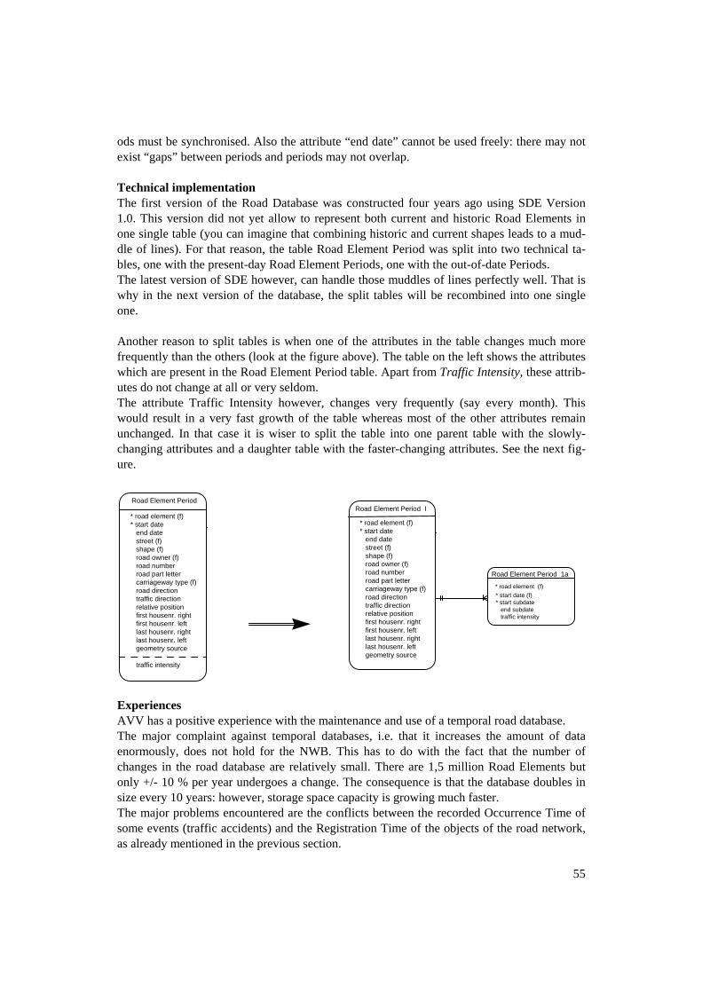
ods must be synchronised. Also the attribute “end date” cannot be used freely: there may not exist “gaps” between periods and periods may not overlap. Technical implementation The first version of the Road Database was constructed four years ago using SDE Version 1.0. This version did not yet allow to represent both current and historic Road Elements in one single table (you can imagine that combining historic and current shapes leads to a mud-dle of lines). For that reason, the table Road Element Period was split into two technical ta-bles, one with the present-day Road Element Periods, one with the out-of-date Periods. The latest version of SDE however, can handle those muddles of lines perfectly well. That is why in the next version of the database, the split tables will be recombined into one single one. Another reason to split tables is when one of the attributes in the table changes much more frequently than the others (look at the figure above). The table on the left shows the attributes which are present in the Road Element Period table. Apart from Traffic Intensity, these attrib-utes do not change at all or very seldom. The attribute Traffic Intensity however, changes very frequently (say every month). This would result in a very fast growth of the table whereas most of the other attributes remain unchanged. In that case it is wiser to split the table into one parent table with the slowly-changing attributes and a daughter table with the faster-changing attributes. See the next fig-ure.

Road Element Period I

* road element (f)* start date end date street (f) shape (f) road owner (f) road number road part letter carriageway type (f) road direction traffic direction relative position first housenr. right first housenr. left last housenr. right last housenr. left geometry source

Road Element Period 1a

* road element (f)* start date (f) * start subdate end subdate traffic intensity

Road Element Period

* road element (f)* start date end date street (f) shape (f) road owner (f) road number road part letter carriageway type (f) road direction traffic direction relative position first housenr. right first housenr. left last housenr. right last housenr. left geometry source

traffic intensity

Experiences AVV has a positive experience with the maintenance and use of a temporal road database. The major complaint against temporal databases, i.e. that it increases the amount of data enormously, does not hold for the NWB. This has to do with the fact that the number of changes in the road database are relatively small. There are 1,5 million Road Elements but only +/- 10 % per year undergoes a change. The consequence is that the database doubles in size every 10 years: however, storage space capacity is growing much faster. The major problems encountered are the conflicts between the recorded Occurrence Time of some events (traffic accidents) and the Registration Time of the objects of the road network, as already mentioned in the previous section.

55

Future The national road database will be extended in the near future with referential attributes as postal codes and with descriptive attributes as quality of the road surface, number of lanes etc. History will continue to play an important role. Furthermore, users will get a on-line connection to the NWB road database. To start with, this will concern read-only access, but later on, some users may get restricted editing facilities. This might make the treatment of time and history more complicated than today. Time in geographical databases will remain an intriguing and challenging issue.

56

Time in relation to geoscientific data Ipo Ritsema NITG-TNO, P.O. Box 80015, 3508 TA Utrecht, The Netherlands Telephone: 31 (0)30 256 4600 Fax: 31 (0)30 256 4605 E-mail: i.ritsema@nitg.tno.nl Abstract The earth is a complex dynamic system, consisting of many interacting and entangled systems and subsystems. For a sustainable development of our planet it is important to understand the behaviour of these systems under various conditions. At NITG-TNO information is gathered concerning the geo-sphere systems, i.e. in the subsur-face of the Netherlands. The geoscientific information can be subdivided into earth observa-tion data, earth model information and earth-human interaction knowledge. Each of these categories does have somewhat different needs for incorporating time. In earth observations there is normally no ambiguity concerning place and time. All data observed are related to the location of instruments used and the observation time, i.e. a continuous world time. It is how-ever important, for integration and comparison reasons, that absolute (and no relative) space and time co-ordinates are used. The earth models are representing the earth systems. An inter-pretation step is executed to go from measurements (referencing to continuous space, time and property scales) towards discrete spatio-temporal features representing different earth systems according to certain classification principles. Both static and dynamic models (variant and invariant world time) exist to represent constant and changing aspects of the earth sys-tems considered. The earth models are interpreted, subject to progressive insight and therefor changing over the ‘version’ time. The earth-human interaction knowledge is derived from the earth observation data or earth model information. Example are gas field or aquifer outlines and their volumes in place, and other relevant knowledge important in decision making in relation to the sustainable management of natural resources, geo-space, geo-hazards and geo-environment. The geoscientific information at NITG-TNO is stored in the Databank Information Nether-lands Subsurface (DINO). This database system is being implemented over many years con-taining old and new solutions for above mentioned time problems. Many geoscientific appli-cation systems and visualisation tools work with geoscientific information typically focussing on the spatial and time aspects separately, except for the earth model calibration (history matching) and prediction (simulation) tools, which definitively require an integrated approach towards space and time. In this presentation examples of the concepts of time in the standard data model for oil and gas (POSC/PPDM, 1994-1999) and HistoryVRML (Lutterman, 1999) as well as the currently used tools will be discussed.

57

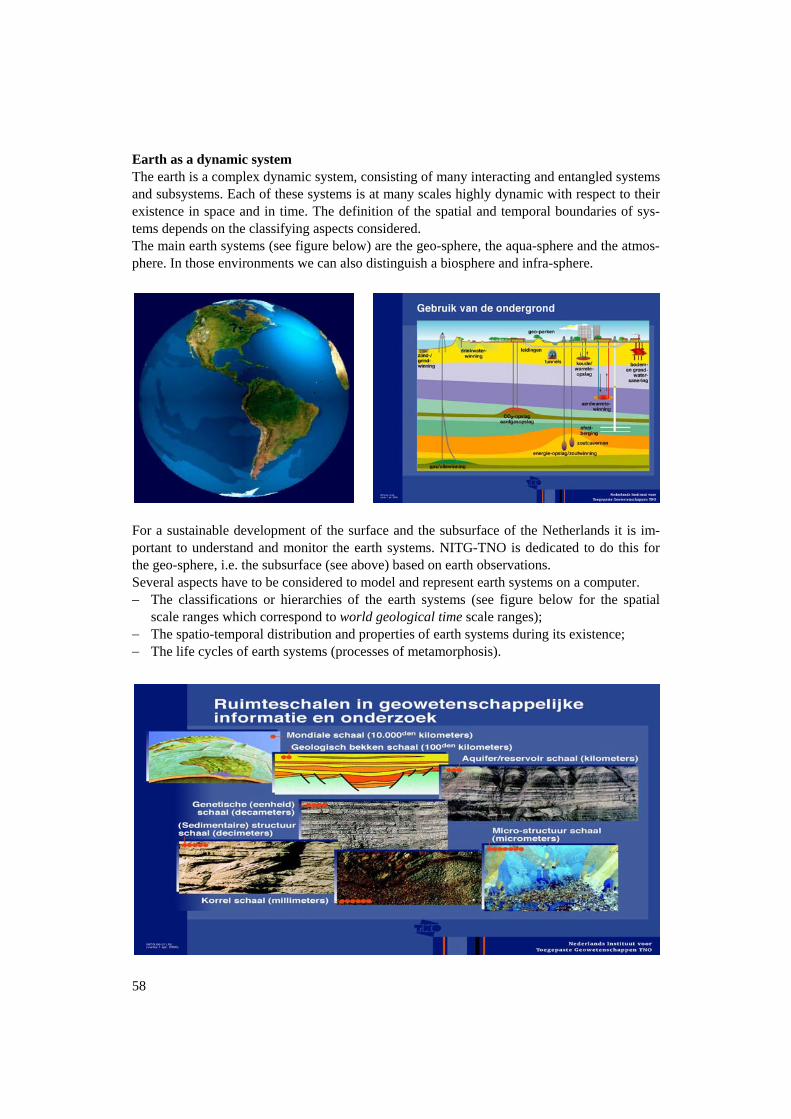
Earth as a dynamic system The earth is a complex dynamic system, consisting of many interacting and entangled systems and subsystems. Each of these systems is at many scales highly dynamic with respect to their existence in space and in time. The definition of the spatial and temporal boundaries of sys-tems depends on the classifying aspects considered. The main earth systems (see figure below) are the geo-sphere, the aqua-sphere and the atmos-phere. In those environments we can also distinguish a biosphere and infra-sphere.

For a sustainable development of the surface and the subsurface of the Netherlands it is im-portant to understand and monitor the earth systems. NITG-TNO is dedicated to do this for the geo-sphere, i.e. the subsurface (see above) based on earth observations. Several aspects have to be considered to model and represent earth systems on a computer. − The classifications or hierarchies of the earth systems (see figure below for the spatial

scale ranges which correspond to world geological time scale ranges); − The spatio-temporal distribution and properties of earth systems during its existence; − The life cycles of earth systems (processes of metamorphosis).

58

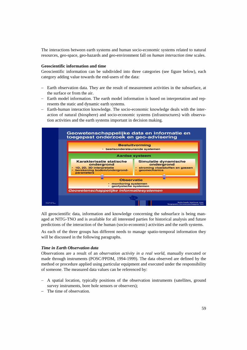
The interactions between earth systems and human socio-economic systems related to natural resources, geo-space, geo-hazards and geo-environment fall on human interaction time scales. Geoscientific information and time Geoscientific information can be subdivided into three categories (see figure below), each category adding value towards the end-users of the data: − Earth observation data. They are the result of measurement activities in the subsurface, at

the surface or from the air. − Earth model information. The earth model information is based on interpretation and rep-

resents the static and dynamic earth systems. − Earth-human interaction knowledge. The socio-economic knowledge deals with the inter-

action of natural (biosphere) and socio-economic systems (infrastructures) with observa-tion activities and the earth systems important in decision making.

All geoscientific data, information and knowledge concerning the subsurface is being man-aged at NITG-TNO and is available for all interested parties for historical analysis and future predictions of the interaction of the human (socio-economic) activities and the earth systems. As each of the three groups has different needs to manage spatio-temporal information they will be discussed in the following paragraphs. Time in Earth Observation data Observations are a result of an observation activity in a real world, manually executed or made through instruments (POSC/PPDM, 1994-1999). The data observed are defined by the method or procedure applied using particular equipment and executed under the responsibility of someone. The measured data values can be referenced by: − A spatial location, typically positions of the observation instruments (satellites, ground

survey instruments, bore hole sensors or observers); − The time of observation.

59

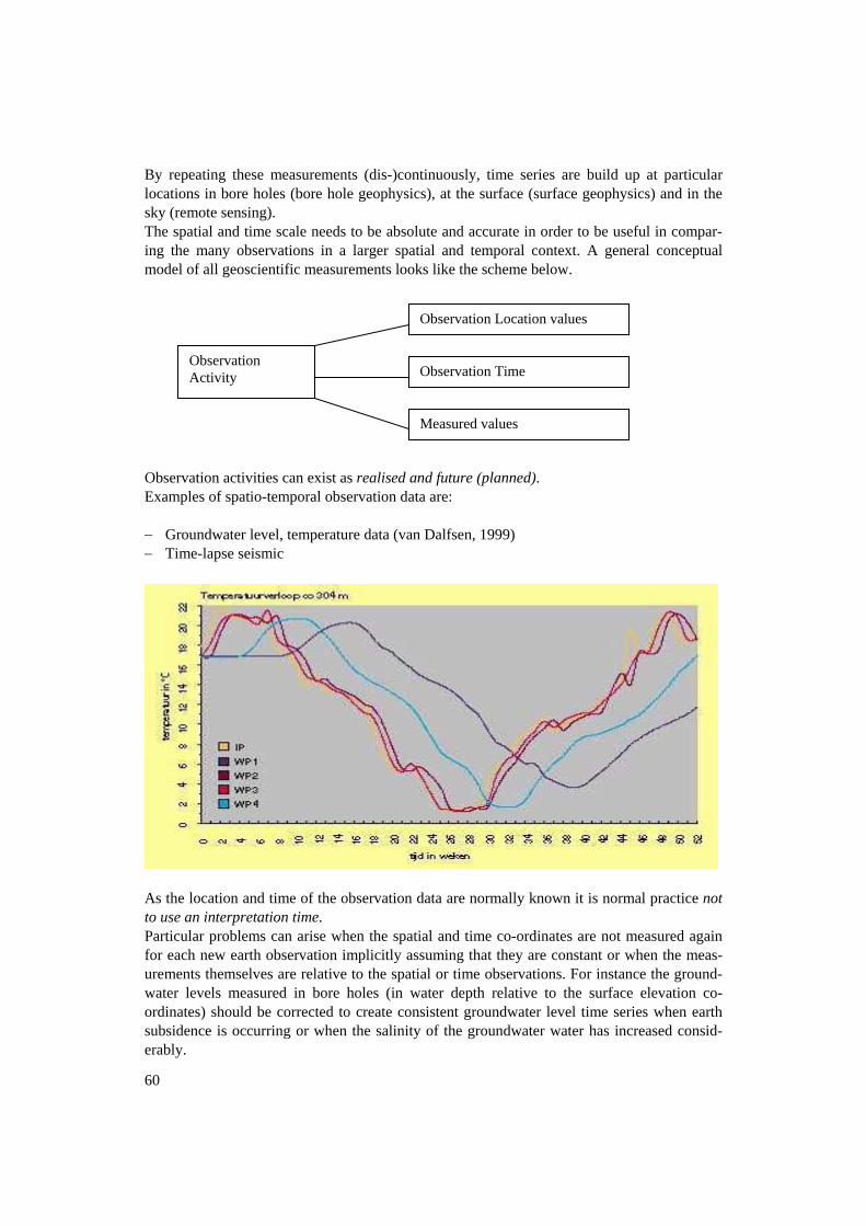
By repeating these measurements (dis-)continuously, time series are build up at particular locations in bore holes (bore hole geophysics), at the surface (surface geophysics) and in the sky (remote sensing). The spatial and time scale needs to be absolute and accurate in order to be useful in compar-ing the many observations in a larger spatial and temporal context. A general conceptual model of all geoscientific measurements looks like the scheme below.

Observation Location values

Observation Time

Measured values

Observation Activity

Observation activities can exist as realised and future (planned). Examples of spatio-temporal observation data are: − Groundwater level, temperature data (van Dalfsen, 1999) − Time-lapse seismic

As the location and time of the observation data are normally known it is normal practice not to use an interpretation time. Particular problems can arise when the spatial and time co-ordinates are not measured again for each new earth observation implicitly assuming that they are constant or when the meas-urements themselves are relative to the spatial or time observations. For instance the ground-water levels measured in bore holes (in water depth relative to the surface elevation co-ordinates) should be corrected to create consistent groundwater level time series when earth subsidence is occurring or when the salinity of the groundwater water has increased consid-erably.

60

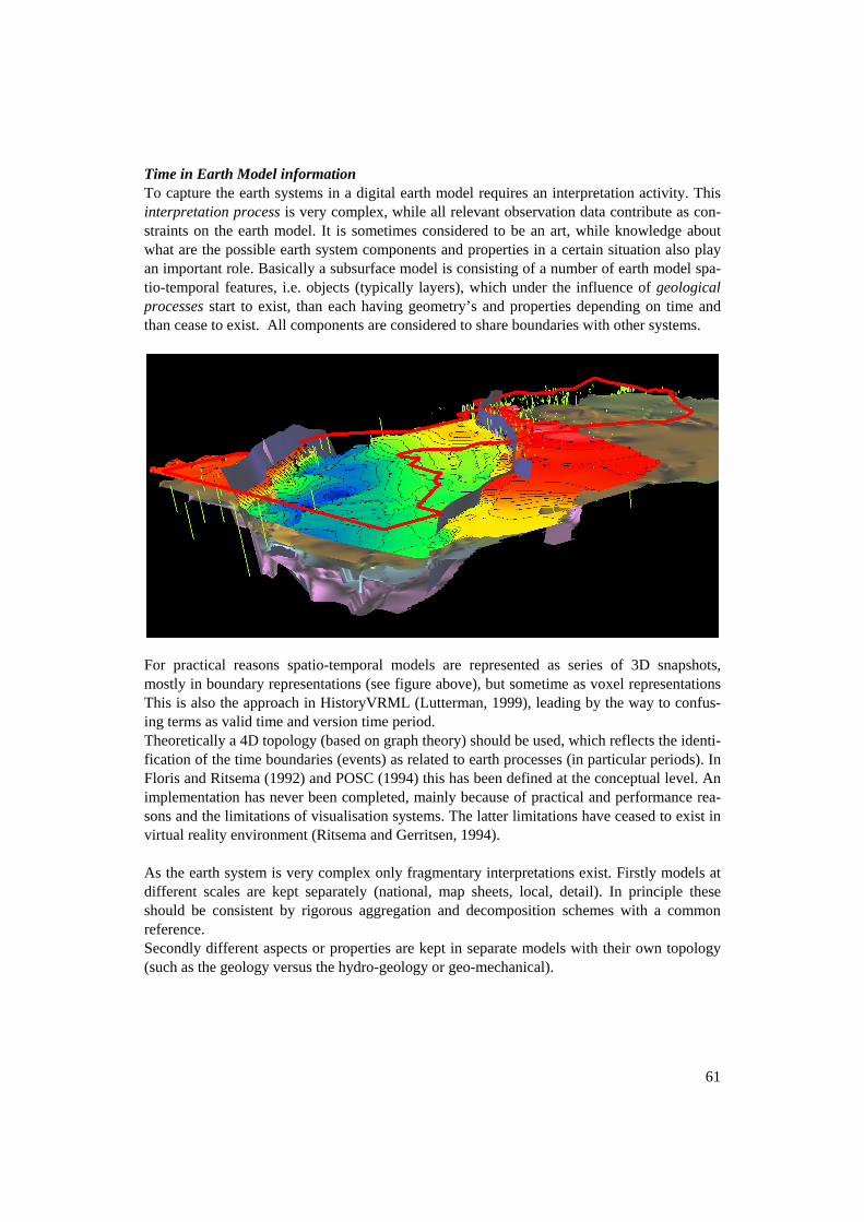
Time in Earth Model information To capture the earth systems in a digital earth model requires an interpretation activity. This interpretation process is very complex, while all relevant observation data contribute as con-straints on the earth model. It is sometimes considered to be an art, while knowledge about what are the possible earth system components and properties in a certain situation also play an important role. Basically a subsurface model is consisting of a number of earth model spa-tio-temporal features, i.e. objects (typically layers), which under the influence of geological processes start to exist, than each having geometry’s and properties depending on time and than cease to exist. All components are considered to share boundaries with other systems. For practical reasons spatio-temporal models are represented as series of 3D snapshots, mostly in boundary representations (see figure above), but sometime as voxel representations This is also the approach in HistoryVRML (Lutterman, 1999), leading by the way to confus-ing terms as valid time and version time period. Theoretically a 4D topology (based on graph theory) should be used, which reflects the identi-fication of the time boundaries (events) as related to earth processes (in particular periods). In Floris and Ritsema (1992) and POSC (1994) this has been defined at the conceptual level. An implementation has never been completed, mainly because of practical and performance rea-sons and the limitations of visualisation systems. The latter limitations have ceased to exist in virtual reality environment (Ritsema and Gerritsen, 1994). As the earth system is very complex only fragmentary interpretations exist. Firstly models at different scales are kept separately (national, map sheets, local, detail). In principle these should be consistent by rigorous aggregation and decomposition schemes with a common reference. Secondly different aspects or properties are kept in separate models with their own topology (such as the geology versus the hydro-geology or geo-mechanical).

61

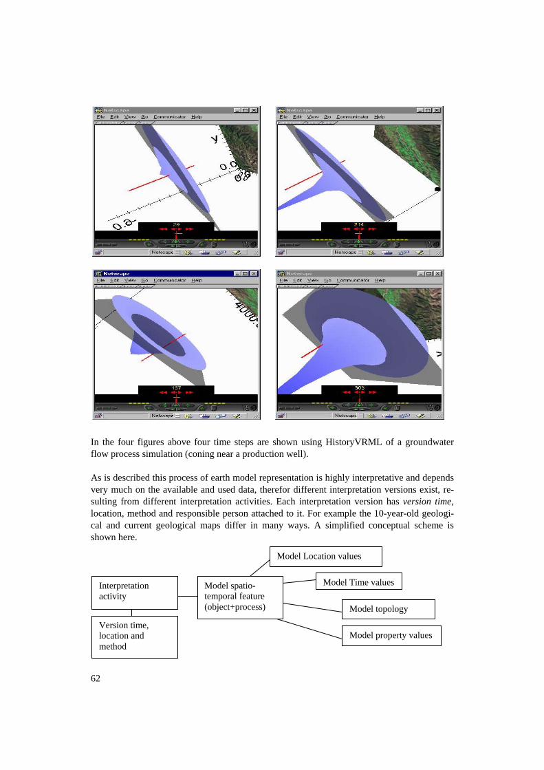
In the four figures above four time steps are shown using HistoryVRML of a groundwater flow process simulation (coning near a production well). As is described this process of earth model representation is highly interpretative and depends very much on the available and used data, therefor different interpretation versions exist, re-sulting from different interpretation activities. Each interpretation version has version time, location, method and responsible person attached to it. For example the 10-year-old geologi-cal and current geological maps differ in many ways. A simplified conceptual scheme is shown here.

Model spatio-temporal feature (object+process)

Model Location values

s

Version time, location and method

Interpretation activity

62

Model Time value

Model property values

Model topology

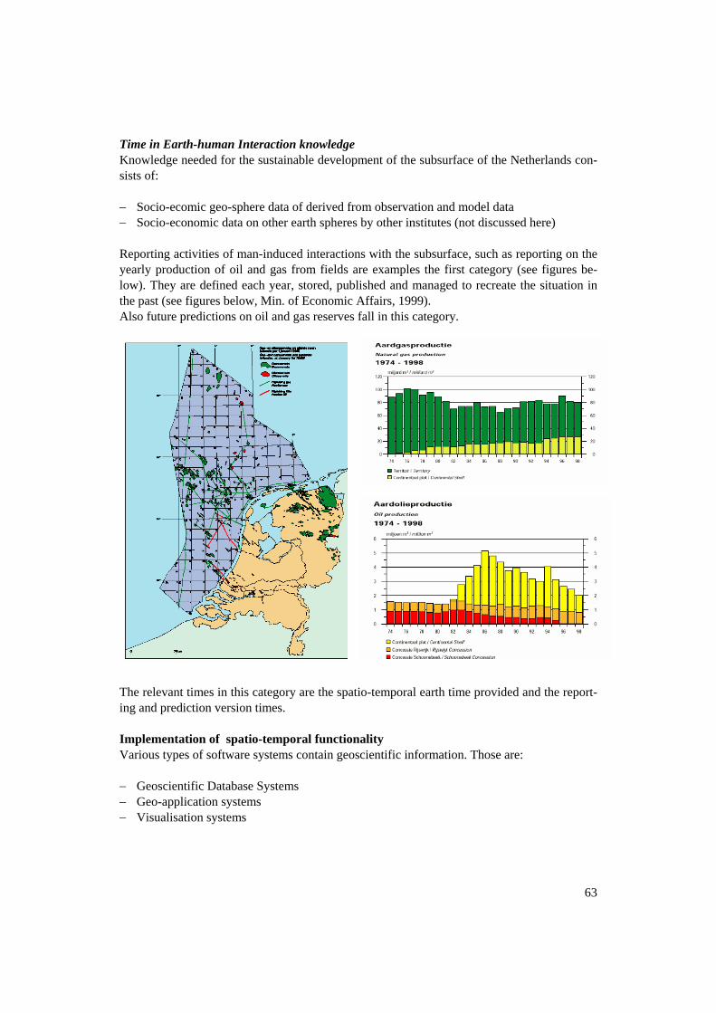
Time in Earth-human Interaction knowledge Knowledge needed for the sustainable development of the subsurface of the Netherlands con-sists of: − Socio-ecomic geo-sphere data of derived from observation and model data − Socio-economic data on other earth spheres by other institutes (not discussed here) Reporting activities of man-induced interactions with the subsurface, such as reporting on the yearly production of oil and gas from fields are examples the first category (see figures be-low). They are defined each year, stored, published and managed to recreate the situation in the past (see figures below, Min. of Economic Affairs, 1999). Also future predictions on oil and gas reserves fall in this category. The relevant times in this category are the spatio-temporal earth time provided and the report-ing and prediction version times. Implementation of spatio-temporal functionality Various types of software systems contain geoscientific information. Those are: − Geoscientific Database Systems − Geo-application systems − Visualisation systems

63

Each of these types of software systems needs to be able to work with the earth world time, i.e. the earth observation time, the earth process time and the earth-human system interaction time. Very often for performance reason the co-ordinates are converted by software systems to scaled and projected world co-ordinates. It is indeed not very efficient to visualise a geologi-cal process using a real geological time scale. These concepts are explained clearly in several existing conceptual models. Industry wide or worldwide naming is not clear yet. For instance in HistoryVRML the time concepts ‘real time’, version (= snapshot), and valid time (= period) are used. Confusion arises also as His-toryVRML calls the scaled time used in visualisation the real time. The software system time is associated with execution time of data digitisation, application runs and visualisation scenes. It is very important not to confuse these with the version time which represents progressing insight in the earth systems. Conclusion The main conclusion is that conceptual models for modelling spatio-temporal geoscientific data have become maturer in the last decade. Three different time concepts are needed in the context of geoscientific data: 1. Earth World Time (= observation time, = geological time, = human interaction time) 2. Version time (= not used in measurements, = interpretation time, = reporting/prediction

time) 3. Software System Time (= data management time, = application time, = visualisation time). These concepts are clear in several existing conceptual models. Industry wide or world wide naming is not clear yet. Great differences exist in VRMLHistory, POSC/PPDM and other contexts. The practical implementation of spatio-temporal models is hindered by a lack of for efficient and affordable solutions, which are based on sound conceptual models. The main bottlenecks are: 1. A sound reference model for spatio-temporal models is needed avoiding naming confu-

sion. 2. Versioning of interpretations is not an easy problem 3. 4D moxel (movie pixel) and 4D topological boundary representation tools is hardly exist-

ing and of those existing the performance is poor. I hope that with all expertise on relevant disciplines available in the Netherlands we are able to progress and contribute not only with Dutch data but also with methodology to support the Al Gore initiative of a Digital Earth.

64

References Berkhout, A.J., Smeets, G. and Ritsema, I.L.; 1991. A strategy for developing a standard E&P data model. The Leading Edge of Exploration, 1991. Chronochorus project; 1998, http://www.dbdet.ece.ntua.gr/~choros/summary.html Dalfsen, W. van, 1999, Temperatuur geeft stroombanen aan, Informatie NITG-TNO, http://www. nitg.tno.nl/eng/pubrels/infor_matie/inf_archief/inf_0399/inf_temp Floris, F.J. and Ritsema, I.L.; 1993. Spatio-temporal (4D), dynamic earth models. EAEG Con-gress, Stavanger GerritsenB.H.M., Ritsema, I.L. 1997, Hyper spatial shapes, NATO-ASI workshop in Rolduc. Gore, A., 1998, The digital Earth: Understanding our planet in the 21st century, Vice president USA. Lutterman, H., Grauer, M.; 1999, VRML History: Storing and browsing temporal 3D worlds, VRML99 Conference Lutterman, H., Grauer, M.; 1999, Using interactive, temporal visualisations for WWW-based pres-entation and exploration of spatio-temporal data, University of Siegen, website http://www-info. uni-siegen.de/winfo/english NITG-TNO, 1999, Databank Informatie Nederlandse Ondergrond, http://www.nitg.tno.nl/eng/ index.shtml NITG-TNO, 1999, Geological Atlas of the deep subsurface of the Netherlands Map sheet XV. Utrecht. Ministry of Economic Affairs, 1999, Oil and Gas activities in 1999, Min-EZ, Den Haag. Mulder, M.M., Ritsema, I.L.; 1990, Exhange format for optimal transfer of geological and geo-physical subsurface data, ISBN 1 85333 622 X, European Oil and Gas conference, Palermo. Oosterom, P. van; 1997, Maintaining consistent topology including historical data in a large scale spatial database, Auto-carto conference, Seattle. POSC, 1994-1999, The Epicentre datamodel for the petroleum industry, Houston, http://www. posc.org/ Ritsema, I.L., Riepen, M., Ridder, J., Paige, S.L. and De Graaf, M.P.; 1988. Online, interactive database system in exploration and production of earth resources. SEG 1988, Anaheim, USA. Ritsema, I.L., Riepen, M, Ridder, J. and De Graaf, M.P.; 1988. Interactive database systems in the petroleum industry, EAEG 1988, The Hague. Ritsema, I.L., Ridder, J.; 1988. Generalised 3-D object structures for geophysical processing and geological interpretation of subsurface models in integrated applications using single exploration and production database, EAEG 1989, Berlin. Ridder, J., Ritsema, I.L.; 1989. Information management: A key to integrating E&P disciplines, World Oil, November 1989. Ritsema, I.L., Ridder, J., Riepen, M. Pen, S.; 1990. A fast object oriented relational DBMS for technical (GIS) applications. EGIS Conference Amsterdam, 1990. Ritsema, I.L. Pen, S.J. and Kemme, Th.; 1991. Logical object model and derived exchange format for 3D subsurface model data. EAEG Congress, Florence.

65

Ritsema, I.L., Gerritsen, B.H.M.; 1994, Construction, visualisation and manipulation of static (3D) and dynamic (4D) Earth Modelling using Virtual Reality tools; paper presented at EAEG/SEG summer workshop Zijl, W., Rijpsma, G. and Ritsema, I.L.; 1996, Upscaling of laboratory-scale rock-mechanical parameters: the emergence of large scale anisotropy, Conference in Geology, Amsterdam. Eijs, R. van, Zijl, W., Voncken, F. and Ritsema, I.L.; 1996, Numerical modelling of subsidence caused by subsurface mining: upscaling and robustness question, Prediction in Geology, Amster-dam. Zijl, W., Rijpsma, G. and Ritsema, I.L.; 1996, Upscaling for geomechanical modelling: non-symmetric rigidity tensors and their symmetric approximation, paper at EAGE conference Am-sterdam.

66