LEV TARASOV

CALCULUSBASIC CONCEPTS FOR HIGH SCHOOLS

MIR PUBLISHERS MOSCOW

Lev Tarasov

Calculus

Mir Publishers Moscow

Translated from the Russian by V. Kisin and A. Zilberman

First published 1988

Revised from the 1984 Russian edition

This electronic version typeset using X ELATEX by Damitr Mazanov.

Released on the web by http://mirtitles.org in 2018.

Contents

Preface v

1 INFINITE NUMERICAL SEQUENCE 1

2 LIMIT OF SEQUENCE 17

3 CONVERGENT SEQUENCE 29

4 FUNCTION 45

5 MORE ON FUNCTION 61

6 LIMIT OF FUNCTION 85

7 MORE ON THE LIMIT OF FUNCTION 103

8 VELOCITY 115

9 DERIVATIVE 129

10 DIFFERENTIATION 147

11 ANTIDERIVATIVE 169

12 INTEGRAL 185

13 DIFFERENTIAL EQUATIONS 199

iii

14 MORE ON DIFFERENTIAL EQUATIONS 215

PROBLEMS 227

iv

Preface

Many objects are obscure to us not because our perceptions arepoor, but simply because these objects are outside of the realm ofour conceptions.

Kosma Prutkov

Confession Of The Author My first acquaintance with calculus (ormathematical analysis) dates back to nearly a quarter of a century. Thishappened in the Moscow Engineering Physics Institute during splendidlectures given at that time by Professor D. A. Vasilkov. Even now I re-member that feeling of delight and almost happiness. In the discussionswith my classmates I rather heatedly insisted on a simile of higher math-ematics to literature, which at that time was to me the most admiredsubject. Sure enough, these comparisons of mine lacked in objectivity.Nevertheless, my arguments were to a certain extent justified. The pres-ence of an inner logic, coherence, dynamics, as well as the use of the mostprecise words to express a way of thinking, these were the characteristicsof the prominent pieces of literature. They were present, in a differentform of course, in higher mathematics as well. I remember that all ofa sudden elementary mathematics which until that moment had seemedto me very dull and stagnant, turned to be brimming with life and innermotion governed by an impeccable logic.

v

Years have passed. The elapsed period of time has inevitably erased thathighly emotional perception of calculus which has become aworking toolfor me. However, my memory keeps intact that unusual happy feelingwhich I experienced at the time of my initiation to this extraordinarilybeautiful world of ideas which we call higher mathematics.

ConfessionOf The ReaderRecently our professor of mathematics toldus that we begin to study a new subject which he called calculus. He saidthat this subject is a foundation of higher mathematics and that it is goingto be very difficult. We have already studied real numbers, the real line,infinite numerical sequences, and limits of sequences. The professor wasindeed right saying that com.. prehension of the subject would presentdifficulties. I listen very carefully to his explanations and during the sameday study the relevant pages of my textbook. I seem to understand every-thing, but at the same time have a feeling of a certain dissatisfaction. It isdifficult forme to construct a consistent picture out of the pieces obtainedin the classroom. It is equally difficult to remember exact wordings anddefinitions, for example, the definition of the limit of sequence. In otherwords, I fail to grasp something very important. Perhaps, all things willbecome clearer in the future, but so far calculus has not become an openbook for me. Moreover, I do not see any substantial difference betweencalculus and algebra. It seems that everything has become rather difficultto perceive and even more difficult to keep in my memory.

Comments Of The Author These two confessions provide an opportu-nity to get acquainted with the two interlocutors in this book. In fact, thewhole book is presented as a relatively free-flowing dialogue between theAUTHOR and the READER. From one discussion to another the AU-THOR will lead the inquisitive and receptive READER to different no-tions, ideas, and theorems of calculus, emphasizing especially complicated

vi

or delicate aspects, stressing the inner logic of proofs, and attracting thereader’s attention to special points. I hope that this form of presentationwill help a reader of the book in learning new definitions such as thoseof derivative, antiderivative, definite integral, differential equation, etc. Ialso expect that it will lead the reader to better understanding of suchconcepts as numerical sequence, limit of sequence, and function. Briefly,these discussions are intended to assist pupils entering a novel world ofcalculus.And if in the long run the reader of the book gets a feeling of theintrinsic beauty and integrity of higher mathematics or even is appealedto it the author will consider his mission as successfully completed.

Working on this book, the author consulted the existing manuals andtextbooks such as Algebra and Elements of Analysis edited by A. N. Kol-mogorov, as well as the specialized textbook by N. Ya. Vilenkin and S.I. Shvartsburd Calculus. Appreciable help was given to the author in theform of comments and recommendations byN.Ya. Vilenkin, B.M. Ivlev,A. M. Kisin, S. N. Krachkovsky, and N. Ch. Krutitskaya, who read thefirst version of the manuscript. I wish to express gratitude for their adviceand interest in my work. I am especially grateful to A. N. Tarasova forher help in preparing the manuscript.

vii

viii

Dialogue 1

INFINITE NUMERICALSEQUENCE

Author: Let us start our discussions of calculus by considering the defi-nition of an infinite numerical sequence or simply a sequence.

We shall consider the following examples of sequences:

1, 2, 4, 8, 16, 32, 64, 128, . . . (1)

5, 7, 9, 11, 13, 15, 17, 19, . . . (2)

1, 4, 9, 16, 25, 36, 49, 64, . . . (3)

1,p

2,p

3, 2,p

5,p

6,p

7, 2p

2, . . . (4)12

,23

,34

,45

,56

,67

,78

,89

, . . . (5)

2, 0, −2, −4, −6, −8, −10, −12, . . . (6)

1,12

,13

,14

,15

,16

,17

,18

, . . . (7)

1,12

, 3,14

, 5,16

, 7,18

, . . . (8)

1

1, −1,13

, −13

,15

, −15

,17

, −17

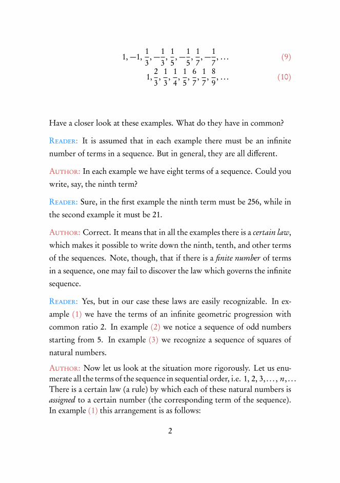
, . . . (9)

1,23

,13

,14

,15

,67

,17

,89

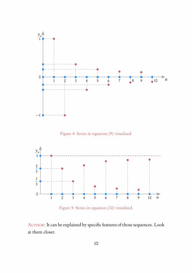
, . . . (10)

Have a closer look at these examples. What do they have in common?

Reader: It is assumed that in each example there must be an infinitenumber of terms in a sequence. But in general, they are all different.

Author: In each example we have eight terms of a sequence. Could youwrite, say, the ninth term?

Reader: Sure, in the first example the ninth term must be 256, while inthe second example it must be 21.

Author: Correct. It means that in all the examples there is a certain law,which makes it possible to write down the ninth, tenth, and other termsof the sequences. Note, though, that if there is a finite number of termsin a sequence, one may fail to discover the law which governs the infinitesequence.

Reader: Yes, but in our case these laws are easily recognizable. In ex-ample (1) we have the terms of an infinite geometric progression withcommon ratio 2. In example (2) we notice a sequence of odd numbersstarting from 5. In example (3) we recognize a sequence of squares ofnatural numbers.

Author: Now let us look at the situation more rigorously. Let us enu-merate all the terms of the sequence in sequential order, i.e. 1, 2, 3, . . . , n, . . .There is a certain law (a rule) by which each of these natural numbers isassigned to a certain number (the corresponding term of the sequence).In example (1) this arrangement is as follows:

2

1 2 4 8 16 32 . . . 2n−1 . . . (terms of the sequence)↑ ↑ ↑ ↑ ↑ ↑ ↑1 2 3 4 5 6 . . . n . . . (position numbers of the terms)

In order to describe a sequence it is sufficient to indicate the term of thesequence corresponding to the number n, i.e. to write down the termof the sequence occupying the nth position. Thus, we can formulate thefollowing definition of a sequence.

Definition

We say that there is an infinite numerical sequence if every naturalnumber (position numbers is unambiguously placed in correspon-dence with a definite number (term of the sequence) by a specificrule.

This relationship may be presented in the following general form:

y1 y2 y3 y4 y5 . . . yn . . .↑ ↑ ↑ ↑ ↑ ↑1 2 3 4 5 . . . n . . .

’The number yn is the nth term of the sequence, and the whole sequenceis sometimes denoted by a symbol (yn ).

Reader: We have been given a somewhat different definition of a se-quence: a sequence is a function defined on a set of natural numbers (in-tegers).

Author: Well, actually the two definitions are equivalent. However, Iam not inclined to use the term “function” too early. First, because thediscussion of a function will come later. Second, you will normally dealwith somewhat different functions, namely those defined not on a set of

3

integers but on the real line or within its segment. Anyway, the abovedefinition of a sequence is quite correct.

Getting back to our examples of sequences, let us look in each case for ananalytical expression (formula) for the nth term. Go ahead.

Reader: Oh, this is not difficult. In example (1) it is yn = 2n. In (2)it is yn = 2n + 3. In (3) it is yn = n2. In (4) it is yn =

pn. In (5) it is

yn = 1− 1n+ 1

=n

n+ 1. In (6) it is yn = 4− 2n. In (7) it is yn =

1n.

In the remaining three examples I just do not know.

Author: Let us look at example (8). One can easily see that if n is an

even integer, then yn =1n, but if n is odd, then yn = n, It means that

yn =

1nif n = 2k

n if n = 2k − 1

Reader: Can I, in this particular case, find a single analytical expressionfor yn?

Author: Yes, you can. Though I think you needn’t. Let us present yn

in a different form:yn = an n+ bn

1n

and demand that the coefficient an be equal to unity if n is odd, and tozero if n is even; the coefficient bn should behave in quite an oppositemanner. In this particular case these coefficients can be determined asfollows:

an =12[1− (−1)n] , bn =

12[1+(−1)n]

Consequently

yn =n2[1− (−1)n]+

12n[1+(−1)n]

4

Do in the same manner in the other two examples.

Reader: For sequence (9) I can write

yn =1

2n[1− (−1)n]+

12(n− 1)

[1+(−1)n]

and for sequence (10)

yn =1

2n[1− (−1)n]+

n2(n+ 1)

[1+(−1)n]

Author: It is important to note that an analytical expression for the nthterm of a given sequence is not necessarily a unique method of defininga sequence. A sequence can be defined, for example, by recursion (orthe recurrence method) (Latin word recurrere means to run back). In thiscase, in order to define a sequence one should describe the first term (orthe first several terms) of the sequence and a recurrence (or a recursion)relation, which is an expression for the nth term of the sequence via thepreceding one (or several preceding terms).

Using the recurrence method, let us present sequence (1), as follows

y1 = 1, yn = 2yn−1

Reader: It’s clear. Sequence (2) can be apparently represented by formu-las

y1 = 5, yn = yn−1+ 2

Author: That’s right. Using recursion, let us try to determine one in-teresting sequence

y1 = 1, y2 = 1, yn = yn−2+ yn−1

5

1, 1, 2, 3, 5, 8, 13, 21, . . . (11)

This sequence is known as the Fibonacci sequence (or numbers).

Reader: I understand, I have heard something about. the problem ofFibonacci rabbits.

Author: Yes, it was this problem, formulated by Fibonacci, the 13thcentury Italian mathematician, that gave the name to this sequence (11).The problem reads as follows. A man places a pair of newly born rabbitsinto a warren and wants to know how many rabbits he would have overa certain period of time. A pair of rabbits will start producing offspringtwo months after they were born and every following month one newpair of rabbits will appear. At the beginning (during the first month) theman will have in his warren only one pair of rabbits (y1 = 1); during thesecond month he will have the same pair of rabbits (y2 = 1); during thethird month the offspring will appear, and therefore the number of thepairs of rabbits in the warren will grow to two (y3 = 3); during the fourthmonth there will be one more reproduction of the first pair (y4 = 3);during the fifth month there will be offspring both from the first andsecond couples of rabbits (y5 = 5), etc. An increase of the number ofpairs in the warren frommonth to month is plotted in Figure 1. One cansee that the numbers of pairs of rabbits counted at the end of each monthform sequence (11), i.e. the Fibonacci, sequence.

Reader: But in reality the rabbits do not multiply in accordance withsuch an idealized pattern. Furthermore, as time goes on, the first pairs ofrabbits should obviously stop proliferating.

Author: The Fibonacci sequence is interesting not because it describesa simplified growth pattern of rabbits’ population. It so happens that

6

Figure 1: Visualising Fibonacci rabbits.

this sequence appears, as if by magic, in quite unexpected situations. Forexample, the Fibonacci numbers are used to process information by com-puters and to optimize programming for computers. However, this is adigression from our main topic.

Getting back to the ways of describing sequences, I would like to pointout that the very method chosen to describe a sequence is not of principalimportance. One sequence may be described, for the sake of convenience,by a formula for the nth term, and another (as, for example, the Fibonaccisequence), by the recurrence method. What is important, however, is themethod used to describe the law of correspondence, i.e. the law by whichany natural number is placed in correspondence with a certain term ofthe sequence. In a number of cases such a law can be formulated only bywords. The examples of such cases are shown below:

2, 3, 5, 7, 11, 13, 17, 19, 23, . . . (12)

3, 3.1, 3.14, 3.141, 3.1415, 3.14159, . . . (13)

7

In both cases we cannot indicate either the formula for the- nth term orthe recurrence relation. Nevertheless, you can without great difficultiesidentify specific laws of correspondence and put them in words.

Reader: Wait a minute. Sequence (12) is a sequence of prime numbersarranged in an increasing order, while (13) is, apparently, a sequence com-posed of decimal approximations, with deficit, for π.

Author: You are absolutely right.

Reader: It may seem that a numerical sequence differs from a random setof numbers by a presence of an intrinsic degree of order that is reflectedeither by the formula for tho nth term or by the recurrence relation.However, the last two examples show that such a degree of order needn’t.be present.

1 2 3 4 5 6 7 8 9 100

1

2

3

yn

n

Figure 2: Graph of the series (4).

Author: Actually, a degree of order determined by a formula (an ana-lytical expression) is not mandatory. It is important, however, to havea law (a rule, a characteristic) of correspondence, which enables one torelate any natural number to a certain term of a sequence. In examples(12) and (13) such laws of correspondence are obvious. Therefore, (12)

8

and (13) are not inferior (and not superior) to sequences (1)-(11) whichpermit an analytical description. Later we shall talk about the geometric

1 2 3 4 5 6 7 8 9 100

1

yn

n

Figure 3: Image of the series (5).

image (ormap) of a numerical sequence. Let us take two coordinate axes,x and y. We shall mark on the first axis integers 1, 2, 3, . . . , n, . . . and onthe second axis, the corresponding terms of a sequence, i.e. the num-bers y1, y2, y3, . . . yn, . . .. Then the sequence can be represented by a setof points M (n, yn) on the coordinate plane. For example Figure 2 imagessequence (4), Figure 3 images sequence (5), Figure 4 images sequence (9),and Figure 5 images sequence (10).

As a matter of fact, there are other types of geometry images of a numer-ical sequence. Let us retain, for example only one coordinate y-axis andplot on it points y1, y2, y3, . . . yn, . . . which map the terms of a sequence.In Figure 6 this method of mapping is illustrated for the sequences thathave been shown in Figure 2-Figure 5. One has to admit that the lattermethod is less descriptive in comparison with the former method.

Reader: But in the case of sequences (4) and (5) the seond method looksrather obvious.

9

1 2 3 4 5 6 7 9

−1

0

1yn

n108

Figure 4: Series in equation (9) visualised.

1 2 3 4 5 6 7 8 9 100

1

13

23

yn

n

Figure 5: Series in equation (10) visualised.

Author: It can be explained by specific features of those sequences. Lookat them closer.

10

0 1 2 3 4 y

y4 y9y3y2y1Sequence (4)

0 0.5 0.6 0.8 0.9 1 y

y4 y9y3y2y1Sequence (5)

−1 −0.8 −0.6 −0.4 −0.2 0 0.2 0.4 0.6 0.8 1

yy4 y9y3y2 y1

Sequence (9)y5y6

0 1 n

y1y2

23

13

y3 y4y5 y6y7

Sequence (10)

Figure 6: Mapping the sequences along a line.

Reader: The terms of sequences (4) and (5) possess the following prop-erty: each term is greater than the preceding term

y1 < y2 < y3, . . .< yn < . . .

It means that all the terms are arranged on the y-axis according to theirserial numbers. As far as I know, such sequence, are called increasing.

Author: A more general case is that of non-decreasing sequences pro-vided we add the equality sign to the above series of inequalities.

Definition

A sequence (yn ) is called nondecreasing if

y1 ⩽ y2 ⩽ y3, . . .⩽ yn ⩽ . . .

11

A sequence (yn ) is called non-increasing if

y1 ⩾ y2 ⩾ y3, . . .⩾ yn ⩾ . . .

Non-decreasing and non-increasing sequences come under thename of monotonic sequences.

Please, identify monotonic sequences among examples (1) -(13).

Reader: Sequences (1), (2), (3), (4), (5), (11), (12), and (13) are nonde-creasing, while (6) and (7) are non-increasing. Sequences (8), (9), and (10)are not monotonic.

Author: Let us formulate one more definition.

Definition

A sequence (yn ) is bounded if there are two numbers A and B la-belling the range which encloses all the terms of a sequence

A⩽ yn ⩽ B (n = 1, 2, 3, . . .)

If it is impossible to identify such two numbers (or, in particular, one canfind only one of the two such numbers, either the least or the greatest),such a sequence is unbounded. Do you find bounded sequences amongour examples?

Reader: Apparently, (5) is bounded.

Author: Find the numbers A and B for it.

Reader: A= 1/2, B = 1.

Author: Of course, but if there exists even one pair of A and B , one

12

may find any number of such pairs. You could say, for example, thatA= 0, B = 2, or A=−100, B = 100, etc., and be equally right.

Reader: Yes, but my numbers are more accurate.

Author: From the viewpoint of the bounded sequence definition, mynumbersAand B are not Letter and notworse than yours. However, yourlast sentence is peculiar. What do you mean by saying “more accurate?”

Reader: My A is apparently the greatest of all possible lower bounds,while my B is the least of all possible upper hounds.

Author: The first part of your statement is doubtlessly correct, whilethe second part of it, concerning B , is not so self-explanatory. It needsproof.

Reader: But it seemed rather obvious. Because all the terms of (5) in-crease gradually, and evidently tend to unity, always remaining less thanunity.

Author: Well, it is right. But it is not yet evident that B = 1 is the leastnumber for which yn ⩽ B is valid for all n: I stress the point again: yourstatement is not self-evident, it needs proof.

I shall note also that “self-evidence” of your statement about B = 1 isnothing but your subjective impression; it is not a mathematically sub-stantiated corollary.

Reader: But how to prove that B = 1 is, in this particular case, the leastof all possible upper bounds?

Author: Yes, it can be proved. But let us not move too fast and by allmeans beware of excessive reliance on so-called self-evident impressions.The warning becomes even more important in the light of the fact that

13

the bounded- ness of a sequence does not imply at all that the greatest A

or the least B must be known explicitly.

Now, let us get back to our sequences and find other examples of boundedsequences. .

Reader: Sequence (7) is also bounded (one can easily find A= 0, B = 1).Finally, bounded sequences are (9) (e.g. A= −1, B = 1), (10) (e.g. A=0, B = 1), and (13) (e.g. A = 3, B = 4). The remaining’ sequences areun-bounded.

Author: You are quite right. Sequences (5), (7), (9), (10), and (13) arebounded. Note that (5), (7), and (13) are bounded and at the same timemonotonic. Don’t you feel that this fact is somewhat puzzling?

Reader: What’s puzzling about it?

Author: Consider, for example, sequence (5). Note that each subse-quent term is greater than the preceding one. I repeat, each term! But thesequence contains an infinite number of terms. Hence, if we follow thesequence far enough, we shall see as many terms with increased magni-tude (compared to the preceding term) as we wish. Nevertheless, thesevalues will never go beyond a certain “boundary”, which in this case isunity. Doesn’t it puzzle you?

Reader: Well, generally speaking, it does. But I notice that we add toeach preceding term an increment which gradually becomes less and less.

Author: Yes, it is true. But this condition is obviously insufficient tomake such a sequence bounded. Take, for example, sequence (4). Hereagain the “increments” added to each term of the sequence gradually de-crease; nevertheless, the sequence is not bounded.

14

Reader: We must conclude, therefore, that in (5) these “increments” di-minish faster than in (4).

Author: All the same, you have to agree that it is not immediately clearthat these “increments” may decrease at a rate resulting in the bounded-ness of a sequence.

Reader: Of course, I agree with that.

Author: The possibility of infinite but bounded sets was not known, forexample, to ancient Greeks. Suffice it to recall the famous paradox aboutAchilles chasing a turtle.

Let us assume that Achilles and the turtle are initially separated by a dis-tance of 1 km, Achilles moves to times faster than the turtle. AncientGreeks reasoned like this: during the time Achilles covers 1 km the turtlecovers 100 m. By the timeAchilles has covered these 100 m, the turtle willhave made another 10 m, and before Achilles has covered these 10 m, theturtle will have made 1 m more, and so on. Out of these considerationsa paradoxical conclusion was derived that Achilles could never catch upwith the turtle.

This “paradox” shows that ancient Greeks failed to grasp the fact that amonotonic sequence may be bounded.

Reader: One has to agree that the presence of both the monotonicityand boundedness is something not so simple to understand.

Author: Indeed, this is not so simple. It brings us close to a discussion onthe limit of sequence. The point is that if a sequence is both monotonicand bounded, it should necessarily have a limit.

Actually, this point can be considered as the “beginning” of calculus.

15

16

Dialogue 2

LIMIT OF SEQUENCE

Author: What mathematical operations do you know?

Reader: Addition, subtraction, multiplication, division, involution (rais-ing to a power), evolution (extracting n root), and taking a logarithm ora modulus.

Author: In order to pass from elementary mathematics to higher math-ematics, this “list” should be supplemented with one more mathematicaloperation, namely, that of finding the limit of sequence; this operationis called sometimes the limit transition (or passage to the limit). By theway, we shall clarify below the meaning of the last phrase of the previ-ous dialogue, stating that calculus “begins” where the limit of sequence isintroduced.

Reader: I heard that higher mathematics uses the operations of differen-tiation and integration.

Author: These operations, as we shall see, are in essence nothing but thevariations of the limit transition.

17

Now, let us get down to the concept of the limit of sequence. Do youknow what it is?

Reader: I learned the definition of the limit of sequence. However, Idoubt that I can reproduce it from memory.

Author: But you seem to “feel” this notion somehow? Probably, youcan indicate which of the sequences discussed above have limits and whatthe value of the limit is in each case.

Reader: I think I can do this, The limit is 1 for sequence (5), zero for (7)and (9), and π for (13).

Author: That’s right. The remaining sequences have no limits.

Reader: By the way, sequence (9) is not monotonic . . .

Author: Apparently, you have just remembered the end of our previousdialogue where it was stated that if a sequence is both monotonic andbounded, it has a limit.

Reader: That’s correct. But isn’t this a contradiction?

Author: Where do you find the contradiction? Do you think that fromthe statement “If a sequence is both monotonic and bounded, it has alimit” one should necessarily draw a reverse statement like “If a sequencehas a limit, it must be monotonic and bounded?” Later we shall see that anecessary condition for a limit is only the boundedness of a sequence. Themonotonicity is notmandatory at all; consider, for example, sequence (9).

Let us get back to the concept of the limit of sequence. Since you havecorrectly indicated the sequences that have limits, you obviously havesome understanding of this concept. Could you formulate it?

18

Reader: A limit is a number to which a given sequence tends (converges).

Author: What do you mean by saying “converges to a number”?

Reader: I mean that with an increase of the serial number, the terms ofa sequence converge very closely to a certain value.

Author: What do you mean by saying “very closely”?

Reader: Well, the “difference” between the values of the terms and thegiven number will become infinitely small. Do you think any additionalexplanation is needed?

Author: The definition of the limit of sequence which you have sug-gested can at best be classified as a subjective impression. We have alreadydiscussed a similar situation in the previous dialogue.

Let us see what is hidden behind the statement made above. For thispurpose, let us look at a rigorous definition of the limit of sequence whichwe are going to examine in detail.

Definition

The number a is said to be the limit of sequence (yn ) if for anypositive number ϵ there is a real number N such that for all n >N

the following inequality holds:

| yn − a |< ϵ (14)

Reader: I am afraid, it is beyond me to remember such a definition.

Author: Don’t hasten to remember. Try to comprehend this definition,to realize its structure and its inner logic. You will see that every wordin this phrase carries a definite and necessary content and that no other

19

definition of the limit of sequence could be more succinct (more delicate,even).

First of all, let us note the logic of the sentence. A certain number is thelimit provided that for any ϵ > 0 there is a number N such that for alln > N inequality (14) holds. In short, it is necessary that for any ϵ acertain number N should exist.

Further, note two “delicate” aspects in this sentence. First, the numberN should exist for any positive number ϵ. Obviously, there is an infiniteset of such ϵ. Second, inequality (14) should hold always (i.e. for each ϵ)for all n >N . But there is an equally infinite set of numbers n!

Reader: Now, the definition of the limit has become more obscure.

Author: Well, it is natural. So far we have been examining the definition“piece by piece”. It is very important that the “delicate” features, the“cream”, so to say, are spotted from the very outset. Once you understandthem, everything will fall into place.

In Figure 7(a) there is a graphic image of a sequence. Strictly speaking, thefirst 40 terms have been plotted on the graph. Let us assume that if anyregularity is noted in these 40 terms, we shall conclude that the regularitydoes exist for n > 40.

Can we say that this sequence converges to the number a (in other words,the number a is the limit of the sequence)?

Reader: It seems plausible.

Author: Let us however, act not on the basis of our impressions but onthe basis of the definition of the limit of sequence. So, we want to verifywhether the number a is the limit of the given sequence. What does our

20

0 10 20 30 40

yn

a

n(a)

0 10 20 30 40

2ϵ

a+ ϵ

a− ϵ

yn

a

n(b)

0 10 20 30 40

yn

a

n

2ϵ12ϵ22ϵ3

(c)

Figure 7: Finding limit of a sequence.

definition of the limit prescribe us to do?

Reader: We should take a positive number ϵ.

Author: Which number?

Reader: Probably. it must be small enough,

Author: The words “small enough” are neither here nor there. Thenumber ϵ must be arbitrary.

Thus, we take an arbitrary positive ϵ. Let us have a look at Figure 7and

21

layoff on the y-axis an interval of length ϵ, both upward and downwardfrom the same point a. Now, let us draw through the points y = a+ϵ andy = a − ϵ the horizontal straight lines that mark an “allowed” band forour sequence. If for any term of the sequence inequality (14) holds, thepoints on the graph corresponding to these terms fall inside the “allowed”band. We see in Figure 7(b) that starting from number ϵ, all the termsof the sequence stay within the limits of the “allowed” band, proving thevalidity of (14) for these terms. We, of course, assume that this situationwill realize for all n > 40, i.e. for the whole infinite “tail” of the sequencenot shown in the diagram.

Thus, for the selected ϵ the number N does exist. In this particular casewe found it to be 7.

Reader: Hence, we can regard a as the limit of the sequence.

Author: Don’t you hurry. The definition clearly emphasizes: “for anypositive ϵ”. So far we have analyzed only one value of ϵ. We should takeanother value of ϵ and find N not for a larger but for a smaller ϵ. If forthe second ϵ the search of N is a success, we should take a third, evensmaller ϵ, and then a fourth, still smaller ϵ, etc., repeating each time theoperation of finding N .

In Figure 7(c) three situations are drawn up for ϵ1,ϵ2and ϵ3 (in this caseϵ1 > ϵ2 > ϵ3). Correspondingly, three “allowed” bands are plotted on thegraph. For a greater clarity, each of these bands has its own starting N .We have chosen N1 = 7, N2 = 15, and N3 = 27.

Note that for each selected ϵwe observe the same situation in Figure 7(c):up to a certain n, the sequence, speaking figuratively, may be “indisci-plined” (in other words, some terms may fallout of the limits of the cor-

22

responding “allowed” band). However, after a certain n is reached, a veryrigid law sets in, namely, all the remaining terms of the sequence (their num-ber is infinite) do stay within the band.

Reader: Do we really have to check it for an infinite number of ϵ values?

Author: Certainly not. Besides, it is impossible. We must be sure thatwhichever value of ϵ > 0 we take, there is such N after which the wholeinfinite “tail” of the sequence will get “locked up” within the limits of thecorresponding “allowed” band.

Reader: And what if we are not so sure?

Author: If we are not and if one can find a value of ϵ1 such that it isimpossible to “lock up” the infinite “tail” of the sequencewithin the limitsof its “allowed” hand, then a is not the limit of our sequence.

Reader: And when do we reach the certainty?

Author: We shall talk this matter over at a later stage because it hasnothing to do with the essence of the definition of the limit of sequence.I suggest that you formulate this definition anew. Don’t try to reconstructthe wording given earlier, just try to put it in your own words.

Reader: I’ll try. The number a is the limit of a given sequence if forany positive ϵ there is (one can find) a serial number n such that for allsubsequent numbers (i.e. for the whole infinite “tail” of the sequence)the following inequality holds: | yn − a |< ϵ.Author: Excellent. You have almost repeated word by word the defini-tion that seemed to you impossible to remember.

Reader: Yes, in reality it all has turned out to be quite logical and rathereasy.

23

Author: It is worthwhile to note that the dialectics of thinking wasclearly at work in this case: a concept becomes “not difficult” because the“complexities” built into it were clarified. First, we break up the conceptinto fragments, expose the “complexities”, then examine the “delicate”points, thus trying to reach the “core” of the problem. Then we recom-pose the concept to make it integral, and, as a result, this reintegratedconcept becomes sufficiently simple and comprehensible. In the futurewe shall try first to find the internal structure and internal logic of theconcepts and theorems.

I believe we can consider the concept of the limit of sequence as thor-oughly analyzed. I should like to add that, as a result, the meaning ofthe sentence “the sequence converges to a” has been explained. I remindyou that initially this sentence seemed to you as requiring no additionalexplanations.

Reader: At the moment it does not seem so self-evident any more. True,I see now quite clearly the idea behind it.

Author: Let us get back to examples (5), (7), and (9). Those are thesequences that we discussed at the beginning of our talk. To begin with,we note that the fact that a sequence (yn ) converges to a certain numbera is conventionally written as

limn→∞ yn = a

(it reads like this: “The limit of yn for n tending to infinity is a.”)

Using the definition of the limit, let us prove that

limn→∞

nn+ 1

= 1; limn→∞

1n= 0;

limn→∞

�1

2n[1− (−1)n]− 1

2(n− 1)[1+(−1)n]�= 0

24

You will begin with the first of the above problems.

Reader: I have to prove that

limn→∞

nn+ 1

= 1

I choose an arbitrary value of ϵ, for example, ϵ= 0.1.

Author: I advise you to begin with finding the modulus of |yn − a|.Reader: In this case, the-modulus is���� n

n+ 1− 1����= 1

n+ 1

Author: Apparently ϵ needn’t be specified, at least at the beginning.

Reader: O.K. Therefore. for an arbitrary positive value of ϵ, I have tofind N such that for all n >N the following inequality holds

1n+ 1

< ϵ

Author: Quite correct. Go on.

Reader: The inequality can be rewritten in the form t

n >1ϵ− 1

It follows that the unknown N may be identified as an integral part of1ϵ− 1. Apparently, for all n >N the inequality in question will hold.

Author: That’s right. Let, for example, ϵ= 0.01.

Reader: Then N =1ϵ− 1= 100− 1= 99.

Author: Let ϵ= 0.001.

25

Reader: Then N =1ϵ− 1= 1000− 1= 999.

Author: Let ϵ= 0.00015.

Reader: Then N =1ϵ− 1= 6665.

Author: It is quite evident that for any ϵ (no matter how small) we canfind a corresponding N .

As to proving that the limits of sequences (7) and (9) are zero, we shallleave it to the reader as an exercise.

Reader: But couldn’t the proof of the equality limn→∞

nn+ 1

= 1 be simpli-

fied?

Author: Have a try.

Reader: Well, first I rewrite the expression in the following way:

limn→∞

nn+ 1

= limn→∞

11

n+ 1

Then I take into consideration that with an increase in n, fraction1nwill

tend to zero, and, consequently, can be neglected against unity. Hence,

we may reject1nand have: lim

n→∞11= 1.

Author: In practice this is the method generally used. However one

should note that in this case we have assumed, first, that limn→∞

1n= 0, and,

second, the validity of the following rules

limn→∞

xn

yn

=lim

n→∞ xn

limn→∞ yn

(15)

limn→∞(xn + zn) = lim

n→∞ xn + limn→∞ zn (16)

26

where xn = 1, yn = 1+1n

and zn =1n. Later on we shall discuss these

rules, but at this juncture I suggest that we simply use them to computeseveral limits. Let us discuss two examples.

Example 1 Find limn→∞

3n− 15n− 6

.

Reader: It will be convenient to present the computation in the form:

limn→∞

3n− 15n− 6

= limn→∞

3− 1n

5− 6n

=lim

n→∞

�3− 1

n

�lim

n→∞

�5− 6

n

� = 35

Author: Ok. Example 2 Compute

limn→∞

6n2− 15n2+ 2n− 1

Reader: We write

limn→∞

6n2− 15n2+ 2n− 1

= limn→∞

6n− 1n

5n+ 2− 1n

.

Author: Wait a moment! Did you think about the reason for dividingboth the numerator and denominator of the fraction in the previous ex-ample by n? We did this because sequences (3n−1) and (5n−6) obviouslyhave no limits, and therefore rule (15) fails. However, each of sequences�

3− 1n

�and�

5− 6n

�has a limit.

Reader: I have got your point. It means that in Example 2 I have to di-vide both the numerator and denominator by n2 to obtain the sequences

27

with limits in both. Accordingly we obtain

limn→∞

6n2− 15n2+ 2n− 1

= limn→∞

6− 1n2

5+2n− 1

n2

=lim

n→∞

�6− 1

n2

�lim

n→∞

�5+

2n− 1

n2

�Author: Well, we have examined the concept of the limit of sequence.Moreover, we have learned a little how to calculate limits. Now it is timeto discuss some properties of sequences with limits. Such sequences arecalled convergent.

28

Dialogue 3

CONVERGENT SEQUENCE

Author: Let us prove the following theorem:

Theorem

If a sequence has a limit, it is bounded.

We assume that a is the limit of a sequence (yn ). Now take an arbitraryvalue of ϵ greater than 0. According to the definition of the limit, theselected ϵ can always be related to N such that for all n >N , I yn−a|< ϵstarting with n =N + 1, all the subsequent terms of the sequence satisfythe following inequalities

a− ϵ < yn < a+ ϵ

As to the terms with serial numbers from 1 to N , it is alway possible toselect both the greatest (denoted by B1 ) and the least (denoted by A1)terms since the number of these term is finite.

Now we have to select the least value from a− ϵ and A1 (denoted by A)and the greatest value from a + ϵ and B1 (denoted by B ). It is obvious

29

that A⩽ yn ⩽ B for all the terms of our sequence, which proves that thesequence yn is bounded.

Reader: I see.

Author: Not toowell, it seems. Let us have a look at the logical structureof the proof. We must verify that if the sequence has a limit, there existtwo numbers A and B such that A⩽ yn ⩽ B for each term of the sequence.Should the sequence contain a finite number of terms, the existence ofsuch two numbers would be evident. However, the sequence contains aninfinite number of terms, the fact that complicates the situation.

Reader: Now it is clear! The point is that if a sequence has a limit a, oneconcludes that in the interval from a− ϵ to a+ ϵ we have an infinite setof yn starting from n =N + 1 so that outside of this interval we shall findonly a finite number of terms (not larger than N ).

Author: Quite correct. As you see, the limit “takes care of” all thecomplications associated with the behaviour of the infinite “tail” of a se-quence. Indeed, |yn−a|< ϵ for all n >N , and this is the main “delicate”point of this theorem. As to the first N terms of a sequence, it is essentialthat their set is finite.

Reader: Now it is all quite lucid. But what about ϵ Its value is not preset,we have to select it.

Author: A selection of a value for ϵ affects only N . If you take a smallerϵ, you will get, generally speaking, a larger N . However, the numberof the terms of a sequence which do not satisfy |yn − a| < ϵ will remainfinite.

And now try to answer the question about the validity of t.he conversetheorem: If a sequence is bounded, does it imply it is convergent as well?

30

Reader: The converse theorem is not true. For example, sequence (10)which was discussed in the first dialogue is bounded. However, it has nolimit.

Author: Right you are. We thus come to a corollary:

Corollary

The boundedness of a sequence is a necessary condition for its con-vergence; however, it is not a sufficient condition. If a sequence isconvergent, it is bounded. If a sequence is unbounded, it is defi-nitely non-convergent,

Reader: I wonder whether there is a sufficient condition for the conver-gence of a sequence?

Author: We have already mentioned this condition in the previous dia-logue, namely, simultaneous validity of both the boundedness and mono-tonicity of a sequence. The Weierstrass Theorem states:

Weierstrass Theorem

If a sequence is both bounded and monotonic, it has a limit.

Unfortunately, the proof of the theorem is beyond the scope of this book;we shall not give it. I shall simply ask you to look again at sequences(5), (7), and (13) (see Dialogue One), which satisfy the conditions of theWeierstrass theorem.

Reader: As far as I understand, again the converse theorem is not true.Indeed, sequence (9) (from Dialogue One) has a limit but is not mono-tonic.

Author: That is correct. We thus come to the following conclusion.

31

Conclusion

If a sequence is both monotonic and bounded, it is a sufficient (butnot necessary) condition for its convergence.

Reader: Well, one can easily get confused.

Bounded Sequences

Monotonic Sequences

Convergent SequencesConvergent SequencesA

B

C

D

E

Figure 8: Bounded, monotonic and convergent sequences.

Author: In order to avoid confusion, let us have a look at another il-lustration (Figure 8). Let us assume that all bounded sequences are “col-lected” (as if we were picking marbles scattered on the floor) in an areashaded by horizontal lines, all monotonic sequences are collected in anarea shaded by tilted lines, and, finally, all convergent sequences are col-lected in an area shaded by vertical lines. Figure 8 shows how all theseareas overlap, in accordance with the theorems discussed above (the ac-tual shape of all the areas is, of course, absolutely arbitrary). As followsfrom the figure, the area shaded vertically is completely included into thearea shaded horizontally. It means that any convergent sequence must bealso bounded. The overlapping of the areas shaded horizontally and by

32

tilted lines occurs inside the area shaded vertically. It means that any se-quence that is both bounded and monotonic must be convergent as well. It iseasy to deduce that only five types of sequences are possible. In the fig-ure the points designated by A, B , C , D , and E identify five sequences ofdifferent types. Try to name these sequences and find the correspondingexamples among the sequences discussed in Dialogue One.

Reader: Point A falls within the intersection of all the three areas. Itrepresents a sequence which is at the same time bounded, monotonic, andconvergent. Sequences (5), (7), and (13) are examples of such sequences.

Author: Continue, please.

Reader: Point B represents a bounded, convergent hut non-monotonicsequence. One example is sequence (9).

Point C represents a bounded but neither convergent nor monotonic se-quence. One example of such a sequence is sequence (10).

Point D represents a monotonic but neither convergent nor bounded se-quence. Examples of such sequences are (1), (2), (3), (4), (6), (11), and(12).

Point E is outside of the shaded areas and thus represents it sequence nei-ther monotonic nor convergent nor bounded. One example is sequence(8).

Author: What type of sequence is impossible then?

Reader: There can be no bounded, monotonic, and non-convergent se-quence. Moreover, it is impossible to have both unboundedness and con-vergence in one sequence.

Author: As you see, Figure 8 helps much to understand t.he relationship

33

between such properties of sequences as boundedness, monotonicity, andconvergence.

In what follows, we shall discuss only convergent sequences. We shallprove the following theorem:

Theorem

A convergent sequence has only one limit.

This is the theorem of the uniqueness of the limit. It means that a conver-gent sequence cannot have two or more limits. Suppose the situation iscontrary to the above statement.

Consider a convergent sequence with two limits a1 and a2 and select a

value for ϵ <|a1− a2|

2. Now assume, for example, that ϵ =

|a1− a2|2

.Since a1 is a limit, then for the selected value of ϵ there is N1 such that forall n > N1 the terms of the sequence (its infinite “tail”) must fall insidethe interval 1 (Figure 9). It means that we must have |yn − a1| < ϵ. Onthe other hand, since at is a2 limit there is N2 such that for all n >N2 theterms of the sequence (again its infinite “tail”) must fall inside the interval2. It means that we must have|yn− a2|< ϵ. Hence, we obtain that for allN greater than the largest among N1 and N2 the impossible must hold,namely, the terms of the sequence must simultaneously belong to theintervals 1 and 2. This contradiction proves the theorem. This proofcontains at least two rather “delicate” points. Can you identify them?

Reader: I certainly notice one of them. If a1 and a2 are limits, no mat-ter how the sequence behaves at the beginning, its terms in the long runhave to concentrate simultaneously around a1 and a2 which is, of course,impossible

34

a1 a2

2ϵ 2ϵy

1 2

Figure 9: Proving the uniqueness of the limit.

Author: Correct. But there is one more “delicate” point, namely, nomatter how close a1 and a2 are, the; should inevitably be spaced by asegment (a gap) of a small but definitely nonzero length.

Reader: But it is self-evident.

Author: I agree. However, this “self-evidence” is connected to one morevery fine aspect without which the very calculus could not be developed.As you probably noted, one cannot identify on the real line two neigh-bouring points. If one point is chosen, it is impossible, in principle, topoint out its “neighbouring” point. In other words, no matter how care-fully you select a pair of points on the real line, it is always possible tofind any number of points between the two.

Take, for example, the interval [0,1]. Now, exclude the point 1. You willhave a half-open interval [0,1|. Can you identify the largest number overthis interval?

Reader: No, it is impossible.

35

Author: That’s right. However, if there were a point neighbouring 1,after the removal of the latter this “neighbour” would have become thelargest number. I would like to note here that many “delicate” points andmany “secrets” in the calculus theorems are ultimately associated with theimpossibility of identifying two neighbouring points on the real line, orof specifying the greatest or least number on an open interval of the realline.

But let us get back to the properties of convergent sequences and provethe following theorem:

Theorem

1f sequences (yn ) and ( zn ) are convergent (we denote their limitsby a and b , respectively), a sequence (yn + zn ) is convergent too,its limit being a+ b .

Reader: This theorem is none other than rule (16) discussed in the pre-vious dialogue.

Author: Thats right. Nevertheless, I suggest you try to prove it.

Reader: If we select an arbitrary ϵ > 0, then there is a number N1 suchthat for all the terms of the first sequence with n > N1 we shall have|yn − a| < ϵ. In addition, for the same ϵ there is N2 such that for all theterms of the second sequence with n > N2 we shall have |zn − a| < ϵ.Now we select the greatest among N1 and N2 (we denote it by N ), thenfor all n >N both |yn−a|< ϵ and |zn−a|< ϵ. Well, this is as far as I cango.

Author: Thus, you have established that for an arbitrary ϵ there is N

such that for all n >N both |yn− a|< ϵ and |zn− a|< ϵ simultaneously.

36

And what can you say about the modulus |(yn+ zn)− (a+ b )| (for all n )?I remind you that |A+B |⩽ |A|+ |B |.Reader: Let us look at

|(yn + zn)− (a+ b )|= |(yn − a)+ (zn − b )|⩽ [|yn − a|+ |zn − b |]< (ϵ+ ϵ) = 2ϵ

Author: You have proved the theorem, haven’t you?

Reader: But we have only established that there is N such that for alln >N we have |(yn + zn)− (a+ b )|< 2ϵ. But we need to prove that

|(yn + zn)− (a+ b )|< ϵAuthor: Ah, that’s peanuts, if you forgive the expression. In the case ofthe sequence (yn + zn) you select a value of ϵ, but for the sequences (yn )and ( zn ) you must select a e value of

ϵ

2and namely for this value find N1

and N2.

Thus, we have proved that if the sequences (yn ) and ( zn ) are convergent,the sequence (yn + zn ) is convergent too. We have even found a limit ofthe sum. And do you think that the converse is equally valid?

Reader: I believe it should be.

Author: You are wrong. Here is a simple illustration:

(yn) =12

,23

,14

,45

,16

,67

,18

, . . .

(zn) =12

,13

,34

,15

,56

,17

,78

, . . .

(yn + zn) = 1, 1, 1, 1, 1, 1, 1, . . .

37

As you see, the sequences (yn) and (zn) are not convergent, while thesequence (yn + zn) is convergent, its limit being equal to unity.

Thus, if a sequence (yn + zn) is convergent, two alternatives are possible:

▶ sequences (yn) and (zn) are convergent as well, or

▶ sequences (yn) and (zn) are divergent.

Reader: But can it be that the sequence (yn) is convergent, while thesequence (zn) is divergent?

Author: It may be easily shown that this is Impossible.

To begin with, let us note that if the sequence (yn) has a limit a, thesequence −(yn) is also convergent and its limit is −a. This follows froman easily proved equality

limn→∞(c yn) = c lim

n→∞ yn

where c is a constant. Assume now that a sequence (yn+zn) is convergentto A, and that (yn) is also convergent and its limit is a. Let us apply thetheorem on the sum of convergent sequences to the sequences (yn + zn)and −(yn). As a result, we obtain that the sequence (yn + zn)− (yn), i.e.(zn), is also convergent, with the limit A− a.

Reader: Indeed (zn) cannot be divergent in this case.

Author: Very well. Let us discuss now one important particular caseof convergent sequences, namely, the so-called infinitesimal sequence, orsimply, infinitesimal. This is the name which is given to a convergentsequence with a limit equal to zero. Sequences (7) and (9) from DialogueOne are examples of infinitesimals.

38

Note that to any convergent sequence (yn) with a limit a there corre-sponds an infinitesimal sequence (αn ), where αn = yn − a. That is whymathematical analysis is also called calculus of infinitesimals.

Now I invite you to prove the following theorem:

Theorem

If (yn) is a bounded sequence and (αn ) is infinitesimal, then (ynαn )is infinitesimal as well.

Reader: Let us select an arbitrary ϵ > 0. We must prove that there isN such that for all n > N the terms of the sequence (ynαn ) satisfy theinequality |yn αn|< ϵ).Author: Do you mind a hint? As the sequence (yn) is bounded, one canfind M such that |yn|⩽M for any n.

Reader: Now all becomes very simple. We know that the sequence (αn )is infinitesimal. It means that for any ϵ′ > 0 we can find N such that forall n >N |αn|< ϵ′. For ϵ′, I select ϵM Then, for n >N we have

|yn αn|= |yn| |αn|⩽M |αn|<Mϵ

M= ϵ

This completes the proof.

Author: Excellent. Now, making use of this theorem, it is very easy toprove another theorem:

Theorem

A sequence (yn zn ) is convergent to ab if sequences (yn ) and ( zn )are convergent to a and b , respectively.

Suppose yn = a + αn and zn = b +βn. Suppose also that the sequences

39

(αn ) and (βn ) are infinitesimal. Then we can write:

yn zn = ab + γn where γn = bαn + aβn +αnβn

Making use of the theorem we have just proved, we conclude that thesequences (bαn), (aβn) and (αnβn) are infinitesimal.

Reader: But what justifies your conclusion about the sequence (αnβn)?

Author: Because any convergent sequence (regardless of whether it isinfinitesimal or not) is bounded. From the theorem on the sum of con-vergent sequences we infer that the sequence (yn) is infinitesimal, whichimmediately yields

limn→∞(yn zn) = ab

This completes the proof.

Reader: Perhaps we should also analyze inverse variants in which thesequence (yn zn) is convergent. What can be said in this case about thesequences (yn) and (zn)?

Author: Nothing definite. in the general case. Obviously, one possibil-ity is that (yn) and (zn) are convergent. However, it is also possible, forexample, for the sequence (yn) to be convergent, while the sequence (zn)is divergent. Here is a simple illustration:

(yn) = 1,14

,19

,116

,125

, . . .1n2

, . . .

(zn) = 1, 2, 3, 4, 5, . . . , n, . . .

(yn zn) = 1,12

,13

,14

,15

, . . .1n

, . . .

By the way, note that here we obtain an infinitesimal sequence by multi-plying an infinitesimal sequence by an unbounded sequence. In the gen-eral case, however, such multiplication needn’t produce an infinitesimal.

40

Finally, there is a possibility when the sequence (yn zn) is convergent, andthe sequences (yn) and (zn) are divergent. Here is one example:

(yn) = 1,14

, 3,116

, 5, . . .136

, 7, . . .

(zn) = 1, 2,19

, 4,125

, 6,149

, . . .

(yn zn) = 1,12

,13

,14

,15

,16

,17

, . . .

Now, let us formulate one more theorem:

Theorem

If (yn) and (zn) are sequences convergent to a and b when b ̸= 0,

then a sequence�

yn

zn

�is also convergent, its its limit being

ab.

We shall omit the proof of this theorem,

Reader: And what if the sequence (zn) contains zero terms?

Author: Such terms are possible. Nevertheless, the number of suchterms can be only finite. Do you know why?

Reader: I think, I can guess. The sequence (zn) has a non-zero limit b .

Author: Let us specify b > 0.

Reader: Well, I select ϵ =b2. There must be an integer N such that

|zn − b | < b2for all n > N . Obviously all zn (the whole infinite “tail”

of the sequence) will be positive. Consequently, the zero terms of thesequence (zn) may only be encountered among a finite number of thefirst N terms.

Author: Excellent. Thus, the number of zeros among the terms of (zn)

41

can only be finite. If such is the case, one can surely drop these terms.Indeed, an elimination of any finite number of terms of a sequence does notaffect its properties. For example, a convergent sequence still remains con-vergent, with its limit unaltered. An elimination of a finite number ofterms may only change N (for a given ϵ), which is certainly unimpor-tant.

Reader: It is quite evident to me that by eliminating a finite number ofterms one does not affect the convergence of a sequence. But could anaddition of a finite number of terms affect the convergence of a sequence?

Author: A finite number of new terms does not affect the convergenceof a sequence either. Nomatter howmany new terms are added and whattheir new serial numbers are, one can always find the greatest number N

after which the whole infinite “tail” of the sequence is unchanged. Nomatter how large the number of new terms may be and where you insertthem, the finite set of new terms cannot change the infinite “tail” of the se-quence. And it is the “tail” that determines the convergence (divergence)of a sequence.

Thus, we have arrived at the following:

Conclusion

Elimination, addition, and any other change of a finite number ofterms of a sequence do not affect either its convergence or its limit(if the sequence is convergent).

Reader: I guess that an elimination of an infinite number of terms (forexample, every other term) must not affect the convergence of a sequenceeither.

42

Author: Here you must be very careful. If an initial sequence is con-vergent, an elimination of an infinite number of its terms (provided thatthe number of the remaining terms is also infinite) does not affect eitherconvergence or the limit of the sequence. If, however, an initial sequenceis divergent, an elimination of an infinite number of its terms may, incertain cases, convert the sequence into a convergent one. For example,if you eliminate from divergent sequence (10) (see Dialogue One) all theterms with even serial numbers, you will get the convergent sequence.

1,13

,15

,17

,19

,111

,113

, . . .

Suppose we form from a given convergent sequence two new convergentsequences. The first new sequence will consist of the terms of the initialsequence with odd serial numbers, while the second will consists of theterms with even serial numbers. What do you think are the limits of thesenew sequences?

Reader: It is easy to prove that the new sequences will have the samelimit as the initial sequence.

Author: You are right.

Note that from a given convergent sequence we can form not only twobut a finite number m of new sequences converging to the same limit.One way to do it is as follows. The first new sequence will consist of the1st, (m+ 1)st, (2m+ 1)st, (3m+ 1)st, etc., terms of the initial sequence.The second sequence will consist of the 2nd, (m + 2)nd, (2m + 2)nd,(3m+ 2)nd, etc., terms of the initial sequence.

Similarly we can form the third, the fourth, and other sequences.

In conclusion, let us see how one can “spoil” a convergent sequence byturning it into divergent. Clearly, different “spoiling” approaches are pos-

43

sible. Try to suggest something simple.

Reader: For example, we can replace all the terms with even serial num-bers by a constant that is not equal to the limit of the initial sequence.For example, convergent sequence (5) (see Dialogue One) can be “spoilt”in the following manner:

12

, 2,34

, 2,56

, 2,78

, 2, . . .

Author: I see that you havemastered verywell the essence of the conceptof a convergent sequence. Now we are ready for another substantial step,namely, consider one of the most important concepts in calculus: thedefinition of a function.

44

Dialogue 4

FUNCTION

Reader: Functions are widely used in elementary mathematics.

Author: Yes, of course. You are familiar with numerical functions. More-over, you have worked already with different numerical functions. Nev-ertheless, it will be worthwhile to dwell on the concept of the function.To begin with, what is your idea of a function?

Reader: As I understand it, a function is a certain correspondence be-tween two variables, for example, between x and y. Or rather, it is adependence of a variable y on a variable x.

Author: What do you mean by a “variable”?

Reader: It is a quantity which may assume different values.

Author: Can you explain what your understanding of the expression“a quantity assumes a value” is? What does it mean? And what are thereasons, in particular, that make a quantity to assume this or that value?Don’t you feel that the very concept of a variable quantity (if you are

45

going to use this concept) needs a definition?

Reader: O.K., what if I say: a function y = f (x) symbolizes a depen-dence of y on x, where x and y are numbers.

Author: I see that you decided to avoid referring to the concept of avariable quantity. Assume that x is a number and y is also a number. Butthen explain, please, the meaning of the phrase “a dependence betweentwo numbers”.

Reader: But look, the words “an independent variable” and “a dependentvariable” can be found in any textbook on mathematics.

Author: The concept of a variable is given in textbooks on mathematicsafter the definition of a function has been introduced.

Reader: It seems I have lost my way.

Author: Actually it is not all that difficult “to construct” an image of anumerical function. I mean image, notmathematical definition which weshall discuss later.

In fact, a numerical function may be pictured as a “black box” that gen-erates a number at the output in response to a number at the input. You putinto this “black box” a number (shown by x in Figure 10) and the "blackbox" outputs a new number (y in Figure 10). Consider, for example, thefollowing function:

y = 4x2− 1

If the input is x = 2, the output is y = 15; if the input is x = 3, the outputis y = 35; if the input is x = 10, the output is y = 399, etc.

Reader: What does this “black box” look like? You have stressed thatFigure 10 is only symbolic.

46

“Black Box”Working as aFunction

x

y

Figure 10: A numerical function as a black box.

Author: In this particular case it makes no difference. It does not influ-ence the essence of the concept of a function. But a function can also be“pictured” like this:

422− 1

The square in this picture is a “window” where you input the numbers.Note that there may be more than one “window”. For example,

422− 1|2|+ 1

Reader: Obviously, the function you have in mind is

4x2− 1|x|+ 1

Author: Sure. In this case each specific value should be input into both“windows” simultaneously. “Black box” working as a function Figure 10.

By the way, it is always important to see such a “window” (or “windows”)in a formula describing the function. Assume, for example, that one needsto pass from a function y = f (x) to a function y = f (x − 1) (on a graphof a function this transition corresponds to a displacement of the curve

47

in the positive direction of the x-axis by 1). If you clearly understandthe role of such a “window” (“windows”), you will simply replace in this“window” (these “windows”) x by x−1. Such an operation is Illustratedby Figure 11 which represents the following function

y =4x2− 1|x|+ 1

Obviously, as a result of substitution of x − 1 for x we arrive at a new

4x2− 1|x|+ 1

422− 1|2|+ 1

4(x − 1)2− 1|x − 1|+ 1

|x − 1|

|x − 1|

Figure 11: Change in a function from f (x)→ f (x − 1).

function (new “black box”)

4(2− 1)2− 1|2− 1|+ 1

, y =4(x − 1)2− 1|x − 1|+ 1

Reader: I see. If, for example, we wanted to pass from y = f (x) toy = f�

1x

�, the function pictured in Figure 11 would be transformed as

follows:

y =

4x2− 1

1|x| + 1

48

Author: Correct. Now. try to find y = f (x) if

2 f�

1x

�− f (x) = 3x

Reader: I am at a loss.

Author: As a hint, I suggest replacing x by1x.

Reader: This yields

2 f (x)− f�

1x

�=

3x

Now it is clear. Together with the initial equation, the new equation

forms a system of two equations for f (x) and f�

1x

�:

2 f�

1x

�− f (x) = 3x

2 f (x)− f�

1x

�=

3x

By multiplying all the terms of the second equation by 2 and then addingthem to the first equation, we obtain

f (x) = x +2x

Author: Perfectly true.

Reader: In connection with your comment about the numerical func-tion as a “black box” generating a numerical output in response to a nu-merical input, I would like to ask whether other types of “black boxes”are possible in calculus.

Author: Yes, they are. In addition to the numerical function, we shalldiscuss the concepts of an operator and a functional.

49

number numericalfunction

numericalfunction

numericalfunction

operator functional

number numericalfunction number

Figure 12: Understanding place and role of the numerical function as a mathe-matical tool.

Reader: I must confess I have never heard of such concepts.

Author: I can imagine. I think, however, that Figure 12 will be helpful.Besides, it will elucidate the place and role of the numerical function as amathematical tool. Figure 12 shows that:

▶ a numerical function is a “black box” that generates a number at theoutput in response to a number at the input;

▶ an operator is a “black box” that generates a numerical function at theoutput in response to a numerical function at the input; it is said thatall operator applied to a function generates a new function;

▶ a functional is a “black box” that generates a number at the output inresponse to a numerical junction at the input, i.e. a concrete numberis obtained “in response” to a concrete function.

Reader: Could you give examples of operators and functionals?

Author: Wait a minute. In the next dialogues we shall analyze both

50

the concepts of an operator and a functional. So far, we shall confineourselves to a general analysis of both concepts. Now we get back to ourmain object, the numerical function.

The question is: How to construct a “black box” that generates a numer-ical function.

Reader: Well, obviously, we should find a relationship, or a law, accord-ing to which the number at the “output” of the “black box” could beforecast for each specific number introduced at the “input”.

Author: You have put it quite clearly. Note that such a law could benaturally referred to as the law of numerical correspondence. However,the law of numerical correspondence would not be a sufficient definitionof a numerical function.

Reader: What else do we need?

Author: Do you think that any number could be fed into a specific“black box” (function)?

Reader: I see. I have to define a set of numbers acceptable as inputs ofthe given function.

Author: That’s right. This set is said to be the domain of a function.

Thus, the definition of a numerical function is based on two “corner-stones”;

the domain of a function (a certain set of numbers), and the law of nu-merical correspondence.

According to this law, every number from the domain of a function is placedin correspondence with a certain number, which is called the value of the

51

function; the values form the range of the function.

Reader: Thus, we actually have to deal with two numerical sets. On theone hand, we have a set called the domain of a function and, on the other,we have a set called the range of a function.

Author: At this juncture we have come closest to a mathematical defini-tion of a function which will enable us to avoid the somewhat mysteriousword “black box”.

Look at Figure 13. It shows the function y =p

1− x2. Figure 13 picturestwo numerical sets, namely, D (represented by the interval [−1,1]) andE (the interval [0,1]). For your convenience these sets are shown on twodifferent real lines.

0

D

-1 1

0

E

1

Figure 13: Range and domain of a function.

52

The set D is the domain of the function, and E is its range. Each numberin D corresponds to one number in E (every input value is placed incorrespondence with one output value). This correspondence is shownin Figure 13 by arrows pointing from D to E .

Reader: But Figure 13 shows that two different numbers in D correspondto one number in E .

Author: It does not contradict the statement “each number in D cor-responds to one number in E .” I never said that different numbers in D

must correspond to different numbers in E . Your remark (which actuallystems from specific characteristics of the chosen function) is of no princi-pal significance. Several numbers in D may correspond to one number inE . An inverse situation, however, is forbidden. It is not allowed for onenumber in D to correspond to more than one number in E . I emphasizethat each number in D must correspond to only one (not more!) numberin E .

Now we can formulate a mathematical definition of the numerical func-tion.

Definition

Take two numerical sets D and E in which each element x of D

(this is denoted by x ∈ D ) is placed in one-to-one correspondencewith one element y of E . Then we say that a function y = f (x) isset in the domain D , the range of the function being E . It is saidthat the argument x of the function y passes through D and thevalues of y belong to E .

Sometimes it is mentioned (but more often omitted altogether) that bothD and E are subsets of the set of real numbers R (by definition, R is the

53

real line).

On the other hand, the definition of the function can be reformulatedusing the term “mapping”. Let us return again to Figure 13. Assume thatthe number of arrows from the points of D to the points of E is infinite(just imagine that such arrows have been drawn from each point of D ).Would you agree that such a picture brings about an idea that D ismappedonto E?

Reader: Really, it looks like mapping.

Author: Indeed, this mapping can be used to define the function.

Definition

A numerical function is a mapping of a numerical set D (whichis the domain of the function) onto another numerical set E (therange of this function).

Thus, the numerical function is a mapping of one numerical set onto an-other numerical set. The term “mapping” should be understood as a kindof numerical correspondence discussed above. In the notation y = f (x),symbol f means the function itself (i.e. the mapping), with x ∈ D andy ∈ E .

Reader: If the numerical function is a mapping of one numerical set ontoanother numerical set, then the operator can be considered as a mappingof a set of numerical function onto another set of functions, and the func-tional as a mapping of a set of functions onto a numerical set.

Author: You are quite right.

Reader: I have noticed that you persistently use the term “numerical

54

function” (and I follow suit), but usually one simply says “function”. Justhow necessary is the word “numerical”?

Author: You have touched upon a very important aspect. The pointis that in modern mathematics the concept of a function is substantiallybroader than the concept of a numerical function. As a matter of fact, theconcept of a function includes, as particular cases, a numerical functionas well as an operator and a functional, because the essence in all the threeis a mapping of one set onto another independently of the nature of thesets. You have noticed that both operators and functionals are mappingsof certain sets onto certain sets. In a particular case of mapping of anumerical set onto a numerical set we come to a numerical function. In amore general case, however, sets to be mapped can be arbitrary. Considera few examples.

Example 1 Let D be a set of working days in an academic year, and E aset of students in a class. Using these sets, we can define a function real-izing a schedule for the students on duty in the classroom. In compilingthe schedule, each element of D (every working day in the year) is placedin one-to-one correspondence with a certain element of E (a certain stu-dent). This function is a mapping of the set of working days onto the setof students. We may add that the domain of the function consists of theworking days and the range is defined by the set of the students.

Reader: It sounds a bit strange. Moreover, these sets have finite numbersof elements.

Author: This last feature is not principal.

Reader: The phrase “the values assumed on the set of students” soundssomewhat awkward.

55

Author: Because you are used to interpret “value” as “numerical value”.Let us consider some other examples.

Example 2 Let D be a set of all triangles, and E a set of positive realnumbers. Using these sets, we can define two functions, namely, the areaof a triangle and the perimeter of a triangle. Both functions are mappings(certainly, of different nature) of the set of the triangles onto the set of thepositive real numbers. It is said that the set of all the triangles is the domainof these functions and the set of the positive real numbers is the range ofthese functions.

Example 3 Let D be a set of all triangles, and E a set of all circles. Themapping of D onto E can be either a circle inscribed in a triangle, or acircle circumscribed around a triangle. Both have the set of all the trian-gles as the domain of the function and the set of all the circles as the rangeof the function.

By the way, do you think that it is possible to “construct” an inversefunction in a similar way, namely, to define a function with all the circlesas its domain and all the triangles as its range?

Reader: I see no objections.

Author: No, it is impossible. Because any number of different trianglescan be inscribed in or circumscribed around a circle. In other words, eachelement of E (each circle) corresponds to an Infinite number of differentelements of D (i.e, an infinite number of triangles). It means that thereis no function since no mapping can be realized.

However, the situation can be improved if we restrict the set of triangles.

Reader: I guess I know how to do it. We must choose the set of allthe equilateral triangles as the set D . Then it becomes possible to realize

56

both a mapping of D onto E (onto the set of all the circles) and an inversemapping, i.e. themapping of E onto D , since only one equilateral trianglecould be inscribed in or circumscribed around a given circle.

Author: Very good. I see that, you have grasped the essence of the con-cept of functional relationship. I should emphasize that from the broadestpoint of view this concept is based on the idea of mapping one set of ob-jects onto another set of objects. It means that a function can be realized asa numerical function, an operator, or a functional. As we have establishedabove, a function may be represented by an area or perimeter of a geometri-cal figure, such, as a circle inscribed in a triangle or circumscribed around it,or it may take the form of a schedule of students on duty in a classroom, etc.It is obvious that a list of different functions may be unlimited.

Reader: I must admit that such a broad interpretation of the concept ofa function is very new to me.

Author: As a matter of fact, in a very diverse set of possible functions(mappings), we shall use only numerical functions, operators, and func-tionals. Consequently, we shall refer to numerical functions as simplyfunctions, while operators and functionals will be pointed out specifically.

And now we shall examine the already familiar concept of a numericalsequence as an example of mapping.

Reader: A numerical sequence is, apparently, a mapping of a set of natu-ral numbers onto a different numerical set. The elements of the second setare the terms of the sequence. Hence, a numerical sequence is a particularcase of a numerical function. The domain of a function is represented bya set of natural numbers.

Author: This is correct. But you should bear in mind that later on we

57

shall deal with numerical functions whose domain is represented by thereal line, or by its interval (or intervals), and whenever we mention afunction, we shall imply a numerical function.

In this connection it is worthwhile to remind you of the classification ofintervals. In the previous dialogue we have already used this classification,if only partially.

First of all we should distinguish between the intervals of finite length:

▶ a closed interval that begins at a and ends at b is denoted by [a, b ];the numbers x composing this interval meet the inequalities a ⩽x ⩽ b ;

▶ an open interval that begins at a and ends at b is denoted by ]a, b [;the numbers x composing this interval meet the inequalities a <

x < b ;

▶ a half-open interval is denoted either by ]a, b ] or [a, b [, the formerimplies that a < x ⩽ b , and the latter that a ⩽ x < b .

The intervals may also be infinite:

] −∞,∞ [ (−∞< x <∞) the real line]a,∞ ] (a < x <∞)[a,∞ [ (a ⩽ x <∞)] −∞, b [ (−∞< x < b )]−∞, b ] (−∞< x ⩽ b )

Let us consider several specific examples of numerical functions. Judgingby the appearance of the formulas given below, point out the intervals

58

constituting the domains of the following functions:

y =p

1− x2 (17)

y =p

x − 1 (18)

y =p

2− x (19)

y =1p

x − 1(20)

y =1p

2− x(21)

y =p

x − 1+p

2− x (22)

y =1p

x − 1+

1p2− x

(23)

y =p

2− x +1p

x − 1(24)

y =p

x − 1+1p

2− x(25)

Reader: It is not difficult. The domain of function (17) is the interval(−1, 1]; that of (18) is [1,∞[; that of (19) is ]−∞, 2]; that of (20) is]1,∞[; that of (21) is ]∞, 2[; that of (22) is [1,2], etc.

Author: Yes, quite right, but may I interrupt you to emphasize thatif a function is a sum (a difference, or a product) of two functions, itsdomain is represented by the intersection of the sets which are the domainsof the constituent functions. It is well illustrated by function (22). Asa matter of fact, the same rule must be applied to functions (23)-(25).Please, continue.

Reader: The domains of the remaining functions are (23) ]1,2[; (24)]1,2]; (25) [1,2[.

Author: And what can you say about the domain of the function y =px − 2+

p1− x?

59

Reader: The domain of y =p

x − 2 is [2,∞[, while that of y =p

1− xis]−∞, 1]. These intervals do not intersect.

Author: It means that the formula y =p

x − 2+p

1− x does not defineany function.

60

Dialogue 5

MORE ON FUNCTION

Author: Let us discuss the methods of defining functions. One of themhas already been employed quite extensively. I mean the analytical de-scription of a function by some formula, that is, an analytical expression(for example, expressions (17) through (25) examined at the end of thepreceding dialogue).

Reader: As a matter of fact, my concept of a function was practicallyreduced to its representation by a’ formula. It was a formula that I had inmind whenever I spoke about a dependence of a variable y on a variablex.

Author: Unfortunately, the concept of a function as a formula relatingx and y has long been rooted in the minds of students. This is, of course,quite wrong. A function and its formula are very different entities. Itis one thing to define a function as a mapping of one set (in our case itis a numerical set) onto another, in other words, as a “black box” thatgenerates a number at the output in response to a number at the input.

61

It is quite another thing to have just a formula, which represents onlyone of the ways of defining a function. It is wrong to identify a functionwith a formula giving its analytical description (unfortunately, it happenssometimes).

Reader: It seems that after the discussion in the previous dialogue aboutthe function, such identification in a general case is automatically invali-dated. However, if we confine ourselves only to numerical functions andif we bear in mind that working with a function we always use a formulato describe it, a question arises: Why is it erroneous to identify these twonotions? Why should we always emphasize the difference between thefunction and its formula?

Author: I’ll tell you why. First, not every formula defines a function.Actually, at the end of the previous dialogue we already had such an ex-ample. I shall give you some more:

y =1px+

1p−x

y = log x + log (−x),

y =p

sin x − 2,

y = log (sin x − 2), etc.

These formulas do not represent any functions.

Second (and this is more important), not all functions can be written asformulas. One example is the so-calledDirichlet functionwhich is definedon the real line:

y =

1 if x is a rational number

0 if x is an irrational number

Reader: You call this a function?

62

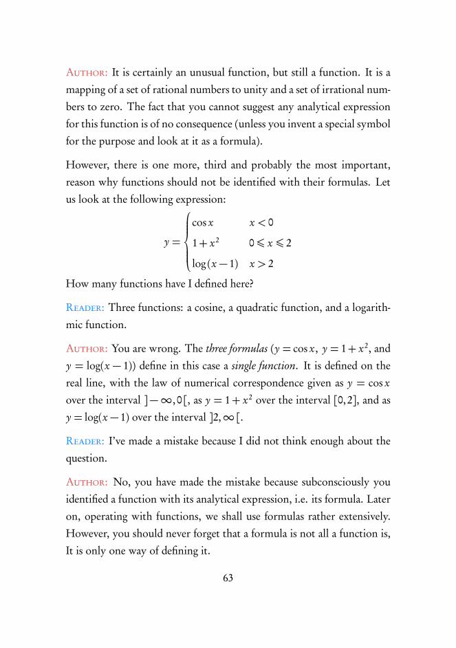
Author: It is certainly an unusual function, but still a function. It is amapping of a set of rational numbers to unity and a set of irrational num-bers to zero. The fact that you cannot suggest any analytical expressionfor this function is of no consequence (unless you invent a special symbolfor the purpose and look at it as a formula).

However, there is one more, third and probably the most important,reason why functions should not be identified with their formulas. Letus look at the following expression:

y =

cos x x < 0

1+ x2 0⩽ x ⩽ 2

log (x − 1) x > 2

How many functions have I defined here?

Reader: Three functions: a cosine, a quadratic function, and a logarith-mic function.

Author: You are wrong. The three formulas (y = cos x, y = 1+ x2, andy = log(x − 1)) define in this case a single function. It is defined on thereal line, with the law of numerical correspondence given as y = cos x

over the interval ]−∞, 0 [, as y = 1+ x2 over the interval [0,2], and asy = log(x − 1) over the interval ]2,∞ [.Reader: I’ve made a mistake because I did not think enough about thequestion.

Author: No, you have made the mistake because subconsciously youidentified a function with its analytical expression, i.e. its formula. Lateron, operating with functions, we shall use formulas rather extensively.However, you should never forget that a formula is not all a function is,It is only one way of defining it.

63

The example above illustrates, by the way, that one should not identifysuch notions as the domain of a function and the range of x on whichan analytical expression is defined (i.e. the domain of an analytical ex-pression). For example, the expression 1+ x2 is defined on the real line.However, in the example above this expression was used to define thefunction only over the interval [0,2].

It should be emphasized that the question about the domain of a functionis of principal significance. It goes without saying that the domain of afunction cannot be wider than the domain of an analytical expressionused to define this function. But it can be narrower.

Reader: Does it mean that a cosine defined, for example, over the inter-val [0,π] and a cosine defined over the interval [π, 3π] are two differentfunctions?

Author: Strictly speaking, it does. A cosine defined, for example, on thereal line is yet another function. In other words, using cosine we may, ifwe wish, define any number of different functions by varying the domainof these functions.

In the most frequent case, when the domain of a function coincides withthe domain of an analytical expression for the function, we speak about anatural domain of the function. Note that in the examples in the previousdialogue we dealt with the natural domains of the functions. A naturaldomain is always meant if the domain of a function in question is notspecified (strictly speaking, the domain of a function should be specifiedin every case).

Reader: It turns out that one and the same function can be described bydifferent formulas and, vice versa, one and the same formula can be used

64

to “construct” different functions.

Author: In the history ofmathematics the realization of this factmarkedthe final break between the concept of a function and that of its analyt-ical expression. This actually happened early in the 19th century whenFourier, t.he French mathematician, very convincingly showed t.hat it isquite irrelevant whether one or many analytical expressions are used todescribe a function. Thereby an end was put to the very long discussionamong mathematicians about. Identifying a function with its analyticalexpression.

It should be noted that similarly to other basic mathematical concepts,the concept of a function went through a long history of evolution. Theterm “function” was introduced by the German mathematician Leibnitzlate in the 17th century. At that time this term had a rather narrowmean-ing and expressed a relationship between geometrical objects. The defi-nition of a functional relationship, freed from geometrical objects, wasfirst formulated early in the 18th century by Bernoulli. The evolutionof the concept of a function can be conventionally broken up into threemain stages. During the first stage (the 18th century) a function was prac-tically identified with its analytical expression. During the second stage(the 19th century) the modern concept of a function started to develop asa mapping of one numerical set onto another. With the development ofthe general theory of sets, the third stage began (the 20th century) whenthe concept of a function formerly defined only for numerical sets wasgeneralized over the sets of an arbitrary nature.

Reader: It appears that by overestimating the role of a formula we in-evitably slip back to the concepts of the 18th century.

Author: Let us discuss nowonemoreway of defining a function, namely,

65

the graphical method. The graph of a function y = f (x) is a set of pointson the plane (x, y) whose abscissas are equal to the values of the indepen-dent variable (x), and whose ordinates are the corresponding values of thedependent variable (y). The idea of the graphical method of defining afunction is easily visualized. Figure 14(a ) plots the graph of the function

y =

cos x x < 0

1+ x2 0⩽ x ⩽ 2

log (x − 1) x > 2

discussed earlier. For a comparison, the graphs of the functions y =cos x, y = 1+ x2, and y = log (x − 1) within their natural domains ofdefinition in tho same figure (cases (b ), (c ), and (d )).

Reader: In Figure 14(a ) I notice an open circle. What does it mean?

Author: This circle graphically represents a point excluded from thegraph. In this particular case the point (2,0) does not belong to the graphof the function. Figure 15 plots the graphs of the functions that werediscussed at the end of the previous dialogue. Let us have a close look atthem.

Reader: Obviously, in all the cases shown in Figure 15 the domain of thefunction is supposed coinciding with the domain of the correspondinganalytical expression.

Author: Yes, you are right. In cases (b ), ( c ), (d ), and (e ) these domainsare infinite intervals. Consequently, only a part of each graph could beshown.

Reader: In other cases, however, such as ( g ), (h ), and ( i ), the domainsof the functions are intervals of finite length. But here as well the figurehas space for only a part of each graph.

66

1 20

y =

cos x x < 0

1+ x2 0⩽ x ⩽ 2

log (x − 1) x > 2

−π−2π

−1

1

−2π −3π2

−π −π2

π

2π 3π

22π

−1

1

0

y = cos x

1

0

y = 1+ x2

Figure 14: The graphs of the functions y = cos x, y = 1+ x2, and y = log (x−1).

Author: That is right. The graph is presented in its complete form onlyin cases (a ) and ( f ). Nevertheless, the behaviour of the graphs is quite

67

Figure 15: A variety of functions and their domains.

68

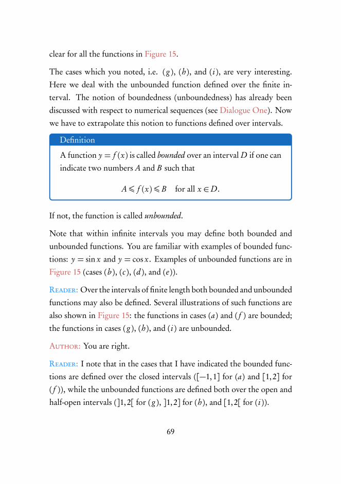
clear for all the functions in Figure 15.

The cases which you noted, i.e. ( g ), (h ), and ( i ), are very interesting.Here we deal with the unbounded function defined over the finite in-terval. The notion of boundedness (unboundedness) has already beendiscussed with respect to numerical sequences (see Dialogue One). Nowwe have to extrapolate this notion to functions defined over intervals.

Definition

A function y = f (x) is called bounded over an interval D if one canindicate two numbers A and B such that

A⩽ f (x)⩽ B for all x ∈D .

If not, the function is called unbounded.

Note that within infinite intervals you may define both bounded andunbounded functions. You are familiar with examples of bounded func-tions: y = sin x and y = cos x. Examples of unbounded functions are inFigure 15 (cases (b ), ( c ), (d ), and ( e )).

Reader: Over the intervals of finite length both bounded and unboundedfunctions may also be defined. Several illustrations of such functions arealso shown in Figure 15: the functions in cases (a ) and ( f ) are bounded;the functions in cases ( g ), (h ), and ( i ) are unbounded.

Author: You are right.

Reader: I note that in the cases that I have indicated the bounded func-tions are defined over the closed intervals ([−1,1] for (a ) and [1,2] for( f )), while the unbounded functions are defined both over the open andhalf-open intervals (]1,2[ for ( g ), ]1,2] for (h ), and [1,2[ for ( i )).

69

Author: This is very much to the point. However, you should bearin mind that it is possible to construct bounded functions defined overopen (half-open) intervals, and unbounded functions defined over closedintervals. Here are two simple illustrations:

Example 1: y = x2 0⩽ x < 2

Example 2:

y =

1x

0⩽ x < 2

1 x = 0

The graphs of these functions are shown in Figure 16.

Figure 16: Examples of bounded functions defined over open (half-open) inter-vals, and unbounded functions defined over closed intervals.

70

Reader: It seems that the boundedness (unboundedness) of a functionand the finiteness of the interval over which it is defined are not interre-lated, Am I right?

Author: Not completely. There is, for example, the following theorem.

Theorem

If a function is defined over a closed interval and if it is monotonic,the function is bounded.

Reader: Obviously, the monotonicity of a function is determined simi-larly to the monotonicity of a numerical sequence.

Author: Yes, it is. Monotonic functions can be classified, as sequences,into non-decreasing and non-increasing:

Definition

A function y = f (x) is said to be non-decreasing over an interval D

it for any x1 and x2 from this interval f (x1)⩽ f (x2) if (x1 ⩽ x2. If,however, f (x1)⩾ f (x2), the function is said to be non-increasing.

Can you prove the theorem formulated above?

Reader: Let the function y = f (x) be defined over the closed interval[a, b ]. We denote f (a) = ya and f (b ) = yb . To make the case morespecific, let us assume that the function is non-decreasing. It means thatya ⩽ yb . I don’t know how to proceed.

Author: Select an arbitrary point x over the interval [a, b ].

Reader: Since a ⩽ x and x ⩽ b , then, according to the condition of theabove theorem, ya ⩽ f (x) and f (x)⩽ yb . Thus, we get that ya ⩽ f (x)⩽

71

yb for all x in the domain of the function. This completes the proof.

Author: Correct. So, if a monotonic function is defined over a closedinterval, it is bounded. As to a non-monotonic function defined over aclosed interval, it may be either bounded (Figure 15(a ) and ( f )) or un-bounded (Figure 15(b )).

And now answer the following question: Is the function y = sin x mono-tonic?

Reader: No, it isn’t.

Author: Well, your answer is as vague as my question. First we shoulddetermine the domain of the function. If we consider the function y =sin x as defined on the natural domain (on the real line), then you are quiteright. If, however, the domain of the function is limited to the intervalh−π

2,π

2

ithe function becomes monotonic (non-decreasing).

Reader: I see that the question of the boundedness or monotonicity ofany function should be settled by taking into account both the type ofthe analytical expression for the function and the interval over which thefunction is defined.

Author: This observation is valid not only for the boundedness ormono-tonicity but also for other properties of functions. For example, is thefunction y = 1− x2 an even function?

Reader: Evidently the answer depends on the domain of the function.

Author: Yes, of course. If the function is defined over an interval sym-metric about the origin of coordinates (for example, on the real line orover the interval [−1,1]), the graph of the function will be symmetricabout the straight line x = 0. In this case y = 1− x2 is an even func-

72

tion. If, however, we assume that the domain of the function is [−1,2],the symmetry we have discussed above is lost (Figure 17) and, as a result,y = 1− x2 is not even.

Figure 17: Is the function y = 1− x2 even?

Reader: It is obvious that your remark covers the case of odd functionsas well.

Author: Yes, it does. Here is a rigorous definition of an even function.

Definition

A function y = f (x) is said to be even if it is defined on a set D

symmetric about the origin and if f (−x) = f (x) for all x ∈D .

By substituting f (−x) =− f (x) for f (−x) = f (x), we obtain the defini-tion of an odd function.

But let us return to monotonic functions. If we drop the equality sign

73

in the definition of a monotonic function (see p. 71) (in f (x1) ⩽ f (x2)or f (x1) ⩽ f (x2)), we obtain a so-called strictly monotonic function. Inthis case a non-decreasing function becomes an increasing function (i.e.f (x1)< f (x2)) . Similarly, a non-increasing function becomes a decreasingfunction (i.e. f (x1) > f (x2) ). In all the previous illustrations of mono-tonic functions we actually dealt with strictly monotonic functions (ei-ther increasing or decreasing). Strictly monotonic functions possess an

Figure 18: Concept of an inverse function.

interesting property: each has an inverse function.

Reader: The concept of an inverse function has already been used in theprevious dialogue in conjunction with the possibility of mapping a set ofequilateral triangles onto a set of circles. We saw that the inverse mapping,i.e. the mapping of the set of circles onto the set of equilateral triangles,was possible.

Author: That’s right. Here we shall examine the concept of an inversefunction in greater detail (but for numerical functions). Consider Fig-

74

ure 18. Similarly to the graphs presented in Figure 13, it shows threefunctions:

(a) y =p

1− x2 −1⩽ x ⩽ 1

(b) y = sin x −π2⩽ x ⩽ π

2(c) y = cos x 0 ⩽ x ⩽πHere we have three mappings of one numerical set onto another. In otherwords, we have three mappings of an interval onto another interval. Incase (a) the interval [−1,1] is mapped onto the interval [0,1]; in (b) theintervalh−π

2,π

2

iis mapped onto the interval [−1,1]; and in (c) the in-

terval [0,π] is mapped onto the interval [−1,1]. What is the differencebetween mappings (b) and (c), on the one hand, and mapping (a), on theother?

Reader: In cases (b) and (c) we have a one-to-one correspondence, i.e.each point of the set D corresponds to a single point of the set E and viceversa, i.e. each point of E corresponds to only one point of D . In case(a), however, there is no one-to-one correspondence.

Author: Yes, you are right. Assume now that the directions of all the ar-rows in the figure are reversed. Now, will the mappings define a functionin all the three cases?

Reader: Obviously, in case (a) we will not have a function since then thereversal of the directions of the arrows produces a forbidden situation,namely, one number corresponds to two numbers. In cases (b) and (c)no forbidden situation occurs so that in these cases we shall have somenew functions.

Author: That is correct. In case (b) we shall arrive at the function y =arcsin x, which is the inverse function with respect to y = sin x defined

75

over the intervalh−π

2,π

2

i.

In case (c) we arrive at the function y = arccos x, which is the inversefunction with respect to y = cos x defined over [0,π].

I would like to place more emphasis on the fact that in order to obtainan inverse function from an initial function, it is necessary to have a one-to-one correspondence between the elements of the sets D and E . Thatis why the functions y = sin x and y = cos x were defined not on theirnatural domains but over such intervals where these functions are eitherincreasing or decreasing. In other words, the initial functions in cases (b)and (c) in Figure 18 were defined as strictly monotonic. A strict mono-tonicity is a sufficient condition for the above-mentioned one-to-one cor-respondence between the elements of D and E . No doubt you can provewithout my help the following theorem.

Theorem

If a function y = f (x) is strictly monotonic, different x are mappedonto different y.

Reader: Thus, a sufficient condition for the existence of the inversefunction- is the strict monotonicity of the initial function. Is this right?

Author: Yes, it is.

Reader: But isn’t the strict monotonicity of the initial function also anecessary condition for the existence of the inverse function?

Author: No, it is not. A one-to-one correspondence may also take place

76

in the case of a non-monotonic function. For example,

y =

1− x 0< x < 1

x 1⩽ x ⩽ 2

Have a look at the graph of this function shown in Figure 19. If a functionis strictly monotonic, it has the inverse function. However, the converseis not true.

Figure 19: A non-monotonic function.

Reader: As I understand it, in order to obtain an inverse function (whenit exists), one should simply reverse the roles of x and y in the equationy = f (x) defining the initial function. The inverse function will thenbe ’given by the equation x = F (y). As a result the range of the initialfunction becomes the domain of the inverse function.

Author: That is correct. In practice a conversion of the initial functionto the inverse function can be easily performed on a graph. The graphof the inverse function is always symmetric to the graph of the initial

77

function about a straight line y = x. It is illustrated in Figure 20, whichshows several pairs of graphs of the initial and inverse functions. A listof some pairs of functions with their domains is given below:

Initial Domain Inverse Domain

(a) x3 −∞< x <∞ 3p

x −∞< x <∞(b ) x2 0⩽ x <∞ p

x 0⩽ x <∞(c) 10x −∞< x <∞ log x 0< x <∞(d ) sin x −π

2⩽ x ⩽ π

2arcsin x −1⩽ x ⩽ 1

(e) cos x 0⩽ x ⩽π arccos x −1⩽ x ⩽ 1

( f ) tan x −π2< x <

π

2arctan x −∞< x <∞

(g ) cot x 0< x <∞ arccot x −∞< x <∞

All the domains of the inverse functions shown in the list case of arethe natural domains of the functions (however, in the case of y = 3

px

the natural domain is sometimes assumed to be restricted to the interval[0,∞[ instead of the whole real line). As to the initial functions, onlytwo of them (y = x3 and y = 10x ) are considered in this case as defined ontheir natural domains. The remaining functions are defined over shorterintervals to ensure the strict monotonicity of the functions.

Now we shall discuss the concept of a composite function.

Let us take as an example the function h(x) =p

1+ cos2 x. Consider alsothe functions f (x) = cos x and g (y) =

p1+ y2.

Reader: This f (x) notation is something new. So far we used to writey = f (x),

78

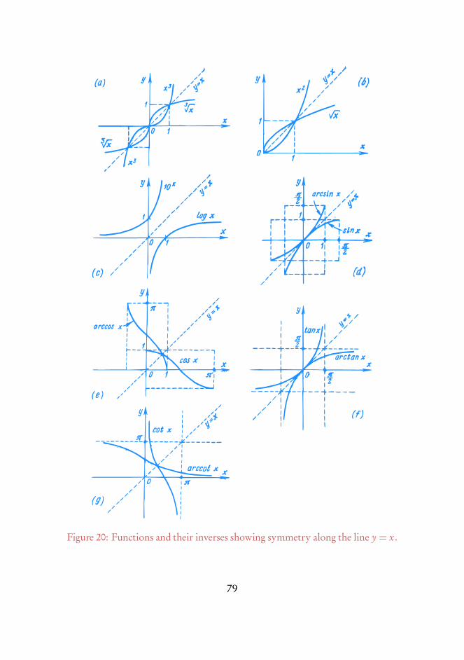
Figure 20: Functions and their inverses showing symmetry along the line y = x.

79

Author: You are right. However, it is expedient to simplify the notation.

Consider the three functions: h(x), f (x), and g (y). The function h(x) isa composite function composed of f (x) and g (y):

h(x) = g [ f (x)]

Reader: I understand. Here, the values of f (x) are used as the values ofthe independent variable (argument) for g (x).

Figure 21: Understanding the composite function.

Author: Let us have a look at Figure 21, which pictures the mappingsof sets in the case of our composite function, h(x) =

p1+ cos2 x, with

f (x) = cos x defined over the interval [0,π].

We see that the function f is a mapping of D (the interval [0,π]) ontoG (the interval [−1,1]), that is, the mapping f . The function g (thefunctionp

1+ y2) is a mapping of G onto E (the interval [1,p

2]), that is,the mapping g . Finally, the function h (the function

p1+ cos2 x defined

over the interval [0,π]) is a mapping of D onto E , that is, the mappingh.

80

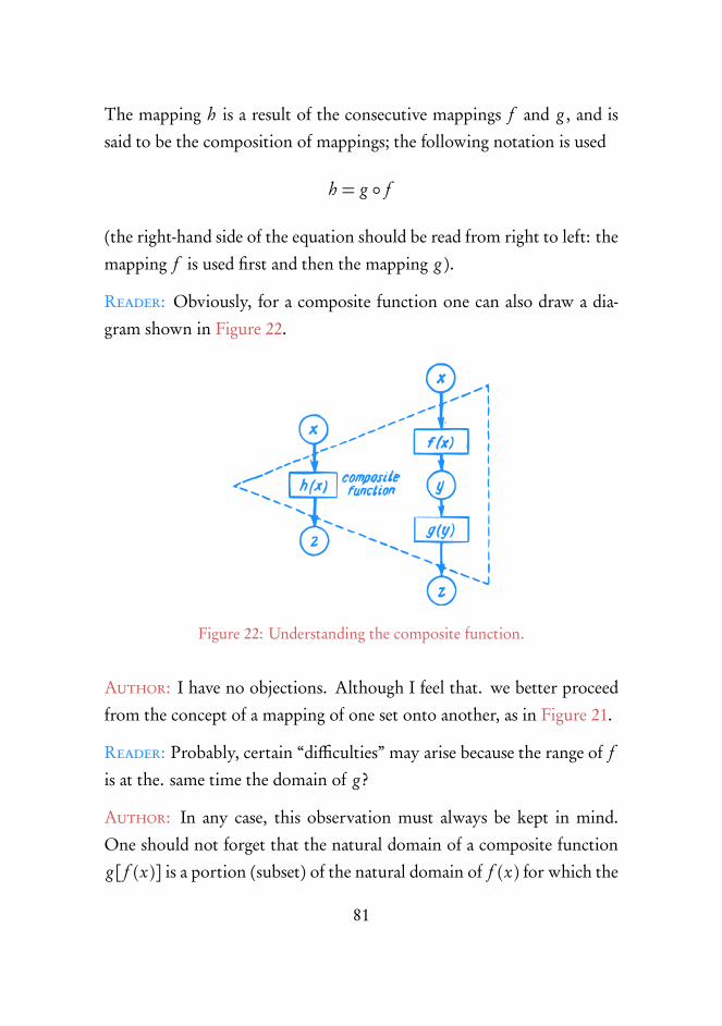
The mapping h is a result of the consecutive mappings f and g , and issaid to be the composition of mappings; the following notation is used

h = g ◦ f

(the right-hand side of the equation should be read from right to left: themapping f is used first and then the mapping g ).

Reader: Obviously, for a composite function one can also draw a dia-gram shown in Figure 22.

Figure 22: Understanding the composite function.

Author: I have no objections. Although I feel that. we better proceedfrom the concept of a mapping of one set onto another, as in Figure 21.

Reader: Probably, certain “difficulties” may arise because the range of f

is at the. same time the domain of g ?

Author: In any case, this observation must always be kept in mind.One should not forget that the natural domain of a composite functiong [ f (x)] is a portion (subset) of the natural domain of f (x) for which the

81

values of f belong to the natural domain of g . This aspect was unim-portant in the example concerning g [ f (x)] =

p1+ cos2 x because all the

values of f (even if cos x is defined on the whole real line) fall into thenatural domain of g (y) =

p1+ y2. I can give you, however, a different

example:

h(x) =Æp

x − 1− 2, f (x) =p

x − 1, g (y) =p

y − 2

The natural domain of f (x) is [1,∞[Not any point in this interval, how-ever, belongs to the domain of the composite function h(x), Since the ex-pressionp

y − 2 is meaningful only if y ⩾ 2, and for y = 2 we have x = 5,the natural domain of this composite function is represented by [5,∞],i.e. a subset smaller than the natural domain of f (x).

Let us examine one more example of a composite function. Consider thefunction y = sin (arcsin x), You know that arcsin x can be regarded as anangle the sine of which is equal to x. In other words, sin(arcsin x) = x,Can you point out the difference between the composite function y =sin (arcsin x) and the function y = x?

Reader: Yes, I can. The natural domain of the function y = x is repre-sented by thewhole real line. As to the composite function y = sin(arcsin x),its natural domain coincides with the natural domain of the functionarcsin x, i.e. with [−1,1]. The graph of the function y = sin(arcsin x)is shown in Figure 23.

Author: Very good. In conclusion, let us get back to the problem of thegraphical definition of a function. Note that there are functions whosegraphs cannot be plotted in principle, the whole curve or a part of it. For

example, it is impossible to plot the graph of the function y = sin1xin

the vicinity of x = 0 (Figure 24). It is also impossible to have the graphof the Dirichlet function mentioned above.

82

Figure 23: The graph of the function y = sin(arcsin x).

Figure 24: The graph of the function y = sin1x.

Reader: It seemed to me that the Dirichlet function had no graph at all.

Author: No, this is not the case. Apparently, your idea of a graph of afunction is always a curve.

Reader: But all the graphs that we have analyzed so far were curves, and

83

rather smooth curves, at that.

Author: In the general case, such an image is not obligatory. But itshould be stressed that every function has its graph, this graph being unique.

Reader: Does this statement hold for functions that are not numerical

Author: Yes, it does. In the most general case we can give the followingdefinition.

Definition

The graph of a function f defined on a set D with a range on a setE is a set of all pairs (x, y) such that the first element of the pair x

belongs to D , while the second element of the pair y belongs to E ,y being a function of x (y = f (x)).

Reader: So it turns out that the graph of a function such as the area ofa circle is actually a set of pairs each consisting of a circle (an elementx ) and a positive number (an element y ) representing the area of a givencircle.

Author: Precisely so. Similarly, the graph of a function representing aschedule of students on duty in a classroom is a set of pairs each containinga date (an element x ) and the name of a student (an element y ) who is onduty on this date. Note also that in practice this function indeed takes agraphic form.

If in a particular case both elements of the pair (both x and y ) are num-bers, we arrive at the graph of the function represented by a set of pointson the coordinate plane. This is the familiar graph of a numerical func-tion.

84

Dialogue 6

LIMIT OF FUNCTION

Author: Consider now the concept of the limit of function.

Reader: But we have already covered rather extensively the concept ofthe limit of a numerical sequence. But a sequence is nothing else but afunction defined on a set of natural numbers. Thus, having discussed thelimit of sequence, we become acquainted with the limit of function aswell. I wonder whether there is any point in a special discussion of theconcept of the limit of function.

Author: Undoubtedly, a further discussion will be very much to thepoint. The functions we are concerned with substantially differ fromsequences (I have already emphasized this fact) because they are definedover intervals and not on sets of natural numbers. This fact makes theconcept of the limit of function specific. Note, for example, that everyspecific convergent sequence has only one limit. It means that the words“the limit of a given sequence” are self-explanatory. As for a functiondefined over an interval, one can speak of an infinite number of “limits”

85

because the limit of function is found for each specific point x = a (or, aswe say, for x tending to a ). Thus the phrase “the limit of a given function”is meaningless because “the limit of a given function must be consideredonly at each given point a”. Besides, this point a should either belongto the domain of the function or coincide with one of the ends of thedomain.

Reader: In this case the definition of the limit of function should be verydifferent from that of the limit of sequence.

Author: Certainly, there is a difference.

Note, first of all, that we analyze a function y = f (x), which is definedover a segment, and a point a in this segment (which may coincide withone of its ends when the function is defined over an open or half-openinterval).

Reader: Do you mean to say that at the point x = a the function f (x)may not be defined at all?

Author: That is quite correct. Now let us formulate the definition ofthe limit of function.

Definition

A number b is said to be the limit of a function f (x) at x tendingto a (the limit at point a ) if for any positive value of ϵ there is apositive value of δ such that for all x satisfying the conditions x

belongs to the domain of the function; x ̸= a and

|x − a|<δ (26)

we have| f (x)− b |< ϵ (27)

86

The standard notation is

limx→a

f (x) = b

Reader: The definition of the limit of function is noticeably longer andmore complicated than that of the limit of sequence.

Author: Note, first of all, that according to (26), point x should belongto the interval ]a − δ,a + δ[. Point x = a should be eliminated fromthis interval. The interval ]a−δ,a+δ[ without point x = a is called apunctured δ -neighbourhood of point a.

We select an arbitrary positive number ϵ. For ϵ we want to find anotherpositive number δ such that the value of the function at any point x fromthe punctured δ-neighbourhood of point a must be inside the interval]b −ϵ, b +ϵ[ (speaking about any point x we imply only the points x inthe domain of the function). If there is such b for any ϵ > 0, b is said tobe the limit of the function at point a. Otherwise, b is not the limit ofthe function at point a.

Reader: And what does your “otherwise” mean in practice?

Author: Assume that the search forδ has been successful for n diminish-ing numbers ϵ1, ϵ2, . . . , ϵn. But then you notice that for a certain numberϵ′ it is impossible to find the required number δ, i.e. for any value of δno matter how small) there is always at least one point x from the punc-tured δ-neighbourhood of point a at which the value of the function liesoutside the interval ]b − ϵ b + ϵ′[.

Reader: But can it happen that we reduce the δ-neighbourhood of pointa so much that not a single point x, belonging to the domain of the func-tion, remains in the δ-neighbourhood?

87

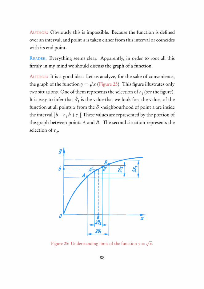
Author: Obviously this is impossible. Because the function is definedover an interval, and point a is taken either from this interval or coincideswith its end point.

Reader: Everything seems clear. Apparently, in order to root all thisfirmly in my mind we should discuss the graph of a function.

Author: It is a good idea. Let us analyze, for the sake of convenience,the graph of the function y =

px (Figure 25). This figure illustrates only

two situations. One of them represents the selection of ϵ1 (see the figure).It is easy to infer that δ1 is the value that we look for: the values of thefunction at all points x from the δ1-neighbourhood of point a are insidethe interval ]b−ϵ1 b+ϵ1[ These values are represented by the portion ofthe graph between points A and B . The second situation represents theselection of ϵ2.

Figure 25: Understanding limit of the function y =p

x.

88

In this case the number that we seek for is δ1: the values of the functionat points x from the δ2-neighbourhood of point a are represented by theportion of the graph between points A′ and B ′.

Reader: Everything you have just described looks so obvious that I seeno “cream”, to use your own words.

Author: “The cream” consists in the following. No matter how small]b − ϵ b + ϵ[ is, one may always select a δ-neighbourhood for point a

such that for all points x in this δ-neighbourhood (all points, with theexception of point a itself and those at which the function is not defined)the values of the function should by all means lie within the indicatedinterval.

Reader: Could you give an example of a function violating this rule?

Author: For instance, the function y = sin1xin the vicinity of point

x = 0. The graph of the function is plotted in Figure 24. Obviously,the smaller is |x| the greater is the frequency with which the graph ofthe function oscillates about the x-axis. For an infinitely small |x| thefrequency of the oscillations tends to infinity. It is easy to prove that the

function y = sin1xhas no limit at x = 0.

Reader: But this function is not defined at zero.

Author: You are right. However, this fact is irrelevant from the view-point of the existence (or absence) of the limit of the function at x = 0.This function is defined over ]−∞, 0[ and ]0,∞[. Point x = 0 is a com-

mon boundary between the intervals over which the function sin1xis

defined.

But let us return to the concept of the limit. Can we, for example, state

89

that b = 0 is the limit of the function sin1xat point x = 0?

Reader: It seems that I get the point. As long as we select ϵ > 1, ev-erything is O.K. But for any ϵ < 1 it becomes impossible to find a δ-neighbourhood of point x = 0 such that at all points x ̸= 0 in this δ-

neighbourhood the values of the function sin1x

are inside the interval]-8, e]. No matter how small the δ-neighbourhood of point x = 0 is, itis the segment of finite length, so that the graph of our function will os-cillate infinitely many times and thus will infinitely many times go beyond]− ϵ, ϵ[.Author: That’s right. Note also that in order to be convinced that a func-tion has no limit, it is sufficient to find a violation even more “modest”.Namely, it is sufficient that the graph of the function leave the interval]− ϵ, ϵ[ at least once for any δ-neighbourhood.Reader: Apparently, not only b = 0 but no other b ̸= 0 can be the limit

of the function y = sin1xat x = 0. Because for any b ̸= 0 we can use the

same arguments as for b = 0.

Author: Hence, we have proved that the function y = sin1xhas no limit

at point x = 0.

Reader: The reason for the absence of the limit at x = 0 lies in oscilla-tions of the graph of the function. These oscillations become more andmore frequent while approaching x = 0.

Author: But the reason is not confined only to the infinitely increasingfrequency of oscillations of the graph. Another reason is the constancyof the amplitude of oscillations. Let us “slightly correct” our function by

multiplying sin1xby x, The graph of the function y = x sin

1xis shown in

90

Figure 26. Do you think that b = 0 is the limit of this function at x = 0?

Figure 26: Finding the limit of the function y = x sin1x.

Reader: I am at a loss.

Author: I’ll answer this question myself. Yes, it is. The proof is withinyour reach if you use the definition of the limit of function. You arewelcome.

Reader: We select an arbitrary ϵ > 0. We should find δ > 0such that����x sin1x− 0����< ϵ for all x (excluding x = 0) satisfying the condition |x −

0|<δ. It seems to me that δ we look for is δ = ϵ.

Author: You are quite right. Because if |x|<δ = ϵ, it becomes evident

that����x sin

1x

����= |x| ����sin 1x

����< ϵ. (since ����sin 1x

����⩽ 1).

91

Reader: Really, the existence of the limit is proved without considerabledifficulties.

Author: But, certainly, not always. Consider, for example, a well-knownfunction y =

px and prove (using the definition of the limit of function)

that b = 1 is the limit of the function at point x = 1. To begin with,consider the following inequality:���px − 1

���< ϵTry to find a function g (ϵ) such that |x − 1| < g (ϵ) for any x satisfyingthe condition��px − 1��< ϵ

Reader: I understand that g (ϵ) is actually the desired δ 6 correspondingto an arbitrary ϵ.

Author: Yes, of course. We begin with some transformations. We shallproceed from the inequality: ���px − 1

���< ϵ (28)

which can be rewritten in the form:

(1− ϵ)<px < (1+ ϵ)

Sincep

x ⩾ 0, the selection of ϵ < 1 a fortiori (which, of course, does notimpair the generality of our proof) allows us to square the last inequalities

(1− ϵ)2 < x < (1+ ϵ)2

On removing the parentheses, we obtain

(−2ϵ− ϵ2)< (x − 1)< (2ϵ+ ϵ2) (29)

92

Note that inequalities (29) are equivalent to (28) (provided that 0 < ϵ <

1). Now let us proceed from (29) to a more exacting inequality:

|x − 1|< (2ϵ− ϵ2) (30)

(since 0 < ϵ < 1, we have (2ϵ − ϵ2) > 0). It is easy to conclude thatif (30) holds, inequalities (29) and, consequently (28) will hold all themore. Thus, for an arbitrary ϵ within 0 < ϵ < 1, it is sufficient to takeδ = 2ϵ− ϵ2

Reader: What happens if ϵ≫ 1?

Author: Then δ determined for any ϵ < 1 will be adequate a fortiori.

Reader: Apparently, we may state that

limx→2

px =p

2, limx→3

px =p

3

and, in general, limx→a

px =p

a.

Author: Yes, that’s right.

Reader: But could we generalize it to

limx→a

f (x) = f (a)

Author: Yes, it is often the case. But not always. Because the func-tion f (x) may be undefined at point a. Remember that the limit of the

function y = x sin1xat point x = 0 is zero, but the function itself is not

defined at point x = 0.

Reader: But perhaps the equality lim f (x) = f (a) x a can be consideredas valid in all the cases when f (x) is defined at point a?

Author: This may not be correct either. Consider, for example, a func-tion which is called the “fractional part of x”. The standard notation for

93

this function is {x}. The function is defined on the whole real line. Weshall divide the real line into half-intervals [n, n+ 1[. For x in [n, n+ 1[we have {x} = x − n. The graph of the function y = {x} is shown inFigure 27.

Figure 27: Graph of the function y = {x}.

Take, for example, x = 1. It is obvious that {x} is defined at point x =1({x}= 0). But does the function have the limit at x = 1?

Reader: It clearly has no limit. In any δ-neighbourhood of point x = 1

there may exist concurrently both the points at which {x} assumes values

greater than, for example,23, and the points at which {x} assumes values

less than13.

It means that neither b = 1 nor b = 0 can be the limit of the functionat point x = 1, if only because it is impossible to find an adequate δ for

ϵ=13.

Author: I see that you have come to be rather fluent in operating withlimits of functions. My compliments.

By the way, you have just proved the theorem on the uniqueness of thelimit of function at a given point.

94

Theorem

A function cannot have two (or more) limits at a given point.

Now let us return to the equality

limx→a

f (x) = f (a) (31)

You already know that there are situations when limx→a

f (x) exists but f (a)does not exist and, vice versa, when f (a) exists but lim

x→af (x) does not

exist. Finally, a situation is possible when both limx→a

f (x) and f (a) exist,but their values are not equal. I’ll give you an example:

f (x) =

x2 if x ̸= 0

1 if x = 0

The graph of this function is shown in Figure 28. It is easy to see thatf (0) = 1, while lim

x→af (x) = 0.

Figure 28: Graph of the function y = f (x), such that f (x) = x2 for x ̸= 0 andf (x) = 1 for x = 0.

95

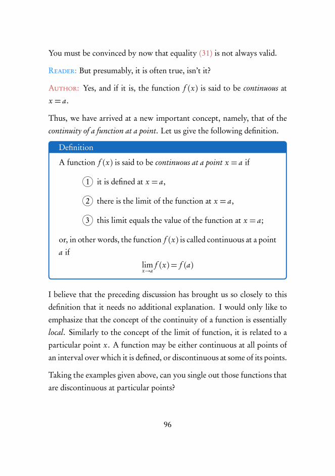
You must be convinced by now that equality (31) is not always valid.

Reader: But presumably, it is often true, isn’t it?

Author: Yes, and if it is, the function f (x) is said to be continuous atx = a.

Thus, we have arrived at a new important concept, namely, that of thecontinuity of a function at a point. Let us give the following definition.

Definition

A function f (x) is said to be continuous at a point x = a if

1 it is defined at x = a,

2 there is the limit of the function at x = a,

3 this limit equals the value of the function at x = a;

or, in other words, the function f (x) is called continuous at a pointa if

limx→a

f (x) = f (a)

I believe that the preceding discussion has brought us so closely to thisdefinition that it needs no additional explanation. I would only like toemphasize that the concept of the continuity of a function is essentiallylocal. Similarly to the concept of the limit of function, it is related to aparticular point x. A function may be either continuous at all points ofan interval over which it is defined, or discontinuous at some of its points.

Taking the examples given above, can you single out those functions thatare discontinuous at particular points?

96

Reader: To beginwith, Imay refer to the functionwhose graph is plottedin Figure 28. This function is discontinuous at x = 0.

Author: Why?

Reader: Because at this point the function assumes the value y = 1,though the limit of the function at this point is apparently zero.

Author: Very good. Can you give other examples?

Reader: The function y = {x} (see Figure 27) is discontinuous at pointsx = 0, ±1, ±2, ±3, . . . The function y = sin

1x(see Figure 24) is discon-

tinuous at x = 0 where it is undefined and, moreover, has no limit. Thefunction whose graph is shown in Figure 14(a ) (see the previous, dia-logue) is discontinuous at x = 2. The function y = tan x is discontinuousat points

x =±π2

, ±3π2

, ±5π2

, ±7π2

Author: That will do. Note that the points at which the continuity ofa function is violated are called discontinuity points. We say that at thesepoints a function has a discontinuity. In passing through a discontinu-ity point a graph of a function manifests a singularity. This fact is wellillustrated by the examples you have just indicated,

Reader: The discontinuity points in all these examples result in an inter-ruption of the curve plotting the function. One exception is the function

y = sin1xsince it is simply impossible to trace a graph of the function at

x = 0.

Author: I may add that neither could you plot the function y = tan x atits discontinuity points (since you cannot draw a line which “goes intoinfinity”).

97

Reader: In any case, if a function is continuous everywhere in the do-main (has no discontinuity points), its graph is a continuous line: it canbe drawn without lifting the pencil from the paper.

Author: I agree. I would like to emphasize that the continuity of a func-tion at a point x guarantees that a very small displacement from this pointwill result in a very small change in the value of the function.

Let us turn to Figure 27 which is the graph of the function y = {x}.Consider, for instance, x = 0.5. The function is continuous at this point.It is quite evident that at a very small displacement from the point (eitherto the left or to the right) the value of the function will also change onlya little. Quite a different situation is observed if x = 1 (at one of thediscontinuity points). At x = 1 the function assumes the value y = 0. Butan infinitesimal shift to the left from the point x = 1 (take, for example,x = 0.999, or x = 0.9999, or any other point no matter how close tox = 1) will bring a sharp change in the value of the function, from y = 0

to y ≈ 1.

Reader: Quite clear. I must admit, however, that the local nature of theconcept of a continuous function (i.e. the fact that the continuity of afunction is always related to a specific point x ) does not quite conform tothe conventional idea of continuity. Because continuity typically impliesa process and, consequently, a sort of an interval. It seems that continuityshould be related not to a specific moment of time, but to an interval oftime.

Author: It is an interesting observation. This local character is a man-ifestation of one of the specific features of calculus. When analyzing afunction at a given point x, you used to speak about its value only at thisspecific point; but calculus operates not only with the value of a function

98

at a point but also with the limit of the function (or its absence) at thispoint, with the continuity of the function at the point. It means that onthe basis of the information about a function at a given point we mayconstruct an image of the behaviour of the function in the vicinity of thispoint. Thus we can predict the behaviour of the function if the point isslightly shifted from x.

So far we have made only the first step in this direction. The next stepwill be the introduction of the concept of a derivative. This will be thesubject of discussion in Dialogues Eight and Nine.

Reader: Nevertheless, I would like to note that in the above examples afunction was found to be either continuous everywhere over any intervalof finite length or discontinuous at a finite number of points. In this sensethe local nature of the concept of a discontinuity point is evident. Thecontinuity of the function, however, is always observed over a certaininterval.

Author: First, the continuity of a function within an interval does notinterfere with the local nature of continuity. A function is continuous overan interval if it is continuous at all points of this interval.

Second, it is not difficult to construct an example in which the numberof discontinuity points over an interval of finite length is infinitely large.Let us look, for example, at the following function:

y =

2 for x =±1, ±12

, ±14

, ±18

, ± 116

. . .

x2 for all the remaining points of the real line, including x = 0

The graph of this function is illustrated in Figure 29. It is easy to concludethat in any δ-neighbourhood of point x = 0 the function has an infinitenumber of discontinuity points.

99

Figure 29: Graph of the function y = f (x), such that f (x) = 2 for x =

±1, ±12

, ±14

, ±18

, ± 116

. . . and f (x) = x2 for all the remaining points of the realline, including x = 0.

Finally, I can give an example of a function which is discontinuous atall points of an infinite interval. This is a function you already know,the Dirichlet function (see the previous dialogue). Being defined on thewhole real line, the function has no limit at any point of the real line;consequently, it is discontinuous at each point.

Reader: This is the reason why we in principle cannot plot the Dirichletfunction by a graph.

Author: As to the most frequent functions, such as power, exponential,logarithmic, trigonometric, and inverse trigonometric, they are continuousat all points of the natural domains of the corresponding analytical expres-

100

sions. The same can be said about composite functions obtained fromthe above elementary functions. The continuity of all these functions isproved in the more advanced courses of calculus. We limit ourselves to amere stating of the fact.

101

102

Dialogue 7

MORE ON THE LIMIT OFFUNCTION

Reader: Comparing the definition of the limit of a function at a pointwith the definition of the limit of a numerical sequence, I come to theconclusion that these two limits are of different nature.

Author: And I understand why. In fact, I did emphasize the differencemyself in the previous dialogue, pointing out, as you probably remem-ber, that a sequence is a function defined on a set of integers, while thefunctions we are discussing at the moment are defined over intervals. Idoubt, however, that you are justified in speaking about the difference inthe nature of the limit of function and that of sequence. In the final anal-ysis (and this is essential) the limit of a function at a point may be definedon the basis of the limit of a numerical sequence.

Reader: This is very interesting.

Author: Let us forget, for the time being, about the definition of the

103

limit of function given in the previous dialogue. Consider a new def-inition. We shall consider, as before, a function, f (x) defined over aninterval, and a point x = a either taken within the interval or coincidingwith its end.

Author: The two are equivalent.

Reader: But in form they are quite different.

Author: We can prove their equivalence. To begin with, let the defini-tion using a δ-neighbourhood of point a be called “definition 1”, and thedefinition using numerical sequences, “definition 2”.

Now, what two theorems must be proved to demonstrate the equivalenceof definitions 1 and 2? Can you formulate these theorems?

Reader: We have to prove two theorems, one direct and the other con-verse. We want to prove that definition 2 follows from definition 1 andvice versa (i.e. definition 1 follows from definition 2).

Author: Correct. First, I shall prove the following theorem.

Theorem

If a number b is the limit of a function f (x) at a point a, in termsof definition 1, it is the limit of the function f (x) at a in terms ofdefinition 2 as well.

Since b is the limit of the function f (x) at point a in terms of definition1 (this is given), consequently, for any ϵ > 0 there is δ > 0 such that| f (x)−b |< ϵ for all x ̸= a from a δ-neighbourhood of point a. Then we“construct” an arbitrary sequence (xn ) , requiring that it be convergentto point a (any xn belong to the domain of the function and xn ̸= a forany n ). As a result we obtain a sequence of the corresponding values of

104

the function (the sequence [ f (xn)]) . We want to prove that the sequence[ f (xn)] is convergent to b .

First, I select an arbitrary ϵ > 0. I should find a number N such that| f (xn)− b |< ϵ for all n >N .

I cannot immediately find such N for an arbitrary ϵ. However, I canindicate for an arbitrary ϵ such δ that | f (x)− b |< ϵ if |x−a|< ϵ. ThenI take this δ and find a sequence (xn) convergent to a. Evidently, since(xn) is convergent to a, ϵ(as any other positive real number) can be placedin correspondence with a number N such that |xn−a|<δ for all n >N .And, consequently, we also have that | f (xn)−b |< ϵ for all n >N . Hencewe find that the thus found number N is actually the desired number. Itproves the convergence of the sequence [ f (xn)] to b . Since the sequence(xn), which is convergent to a was chosen (“constructed”) arbitrarily, weconclude that the theorem’s proof is completed.

If the line of reasoning is clear to you, try briefly to recapitulate the logicalstructure of the proof.

Reader: I shall try to present the structure of the proof as a diagram(Figure 30).

Author: Your diagram is correct. Will you expand on it.

Reader: The first step of the proof: we find for an arbitrary ϵ > 0 anumber δ > 0 such that | f (x)− b |< ϵ if |x − a|<δ.The second step of the proof: we take δ selected at the first step; choose asequence (xn) convergent to a, and find a number N such that |x−a|<δfor all n > N . Having in mind the arguments used at the first step, weconclude that | f (x)− b |< ϵ.

105

Figure 30: Schematic diagram of the proof that two definitions of the limit of afunction are equal.

We have thus found for an arbitrary ϵ > 0 a number N such that | f (xn)−b |< ϵ for all n >N . This completes the proof.

Author: Correct. In conclusion I want to emphasize several essentialpoints on which the proof hinges. We know that | f (x)− b |< ϵ for anyx from the δ-neighbourood of a. Since a sequence (xn) is convergentto a, all xn (the whole infinite “tail” of the sequence (xn) starting froma certain number N + 1) are contained inside the δ-neighbourhood ofpoint a. It then follows that all f (xn) (the whole infinite “tail” of thesequence [ f (xn)] starting from the same number N + 1.) are containedinside the interval ]b − ϵ, b + ϵ[, This proves that the sequence [ f (xn)]converges to b .

Reader: I understand.

Author: Now I am going to prove the following converse theorem.

106

Theorem

If a number b is the limit of a function f (x) at a point a in termsof definition 2, it is also the limit of the function f (x) at a in termsof definition 1.

In this case I shall use the proof by contradiction. Assume the contraryto what is to be proved, namely, assume that b , the limit of f (x) in termsof definition 2, is not, however, the limit of f (x) in terms of definition 1.Can you formulate the last proposition (more exactly, the assumption)?

Reader: As far as I remember, a similar formulation has already beendiscussed in the previous dialogue. If b is not the limit of the functionf (x) at point a (in terms of definition 1), it means that there is ϵ′ > 0

such that it is impossible to find a necessary δ > 0. Namely, no matterwhat δ we select, each time the function f (x)assumes a value outside of]b − ϵ′, b + ϵ′[ for at least one point x from the δ-neighbourhood ofpoint a, i.e. the inequality | f (x)− b |< ϵ′ is violated.Author: Correct. Assume that we have selected precisely this ϵ′ > 0.Next take an arbitrary δ > 0, for instance, δ1 = 1. As you have said, inany δ-neighbourhood of point a and, hence, in the δ-neighbourhood ofthis point there is at least one point x (denoted by x1) such that | f (x1−b |⩾ ϵ′.Reader: What happens if theδ-neighbourhood containsmany such pointsx?

Author: It makes no difference. The important fact is that there is atleast one such point. If there are several such points, take anyone of themand denote it by x1.

107

Now we take a new δ, for instance, δ2 =12. According to our assump-

tion, the δ2-neighbourhood of point a will contain at least one point x

(denoted by x2) such that | f (x2− b |⩾ ϵ′.Further we take δ3 =

13.The δ3-neighbourhood of point a will also con-

tain at least one point x (point x3) such that | f (x3− b |⩾ ϵ′.We can continue this process for a sequence of the δ-neighbourhoods ofpoint a

δ1 = 1, δ2 =12

, δ3 =13

, . . .δn =1n

, . . .

Note that the δ-neighbourhoods are selected in such a way that the se-quence (δn ) converges to zero (is infinitesimal).

If each time we select from each δ-neighbourhood one point x in whichf (x) assumes a value outside of the interval ]b − ϵ′, b + ϵ′[, we obtain asequence composed of points

x1, x3, x3, . . . xn, . . .

Since the sequence (δn ) converges to zero, the sequence (xn) inevitablyconverges to a. A sequence composed of the corresponding values of thefunction (the sequence [ f (xn)] is not convergent to b because for all n wehave | f (xn−b |⩾ ϵ′. It means that we obtained a sequence (xn) convergentto a for which the sequence [ f (xn)] is divergent.

This contradicts the condition of the theorem which states that b is thelimit of the function at a in terms of definition 2. It means that for anysequence (xn) convergent to a the corresponding sequence [ f (xn)must beconvergent to b . And the sequence (xn) that we have found contradictsthis condition.

Hence, the assumption that b , being the limit of the function in terms of

108

definition 2, is not at the same time the limit of the function in terms ofdefinition 1, is invalidated. This completes the proof of the theorem.

Reader: I must admit of being wrong when I spoke about different na-tures, of the limit of numerical sequence and the limit of function at apoint.

Author: These limits differ but their nature is the same. The concept ofthe limit of function at a point is based, as we have seen, on the concept ofthe limit of numerical sequence.

That is why basic theorems about the limits of functions are analogousto those about the limits of sequences.

Reader: We have already noted one of such theorems: the theorem on theuniqueness of the limit of function at a point.

Author: This theorem is analogous to that about the uniqueness of thelimit of numerical sequence.

I shall also give (without proof) the theorems on the limit of the sum; theproduct, and the ratio of functions.

Theorems

If functions f (x) and g (x) have limits at a point a, then functions

[ f (x)+ g (x)] , [ f (x)g (x)] ,�

f (x)g (x)

�also have limits at this point. These limits equal the sum, product,and ratio, respectively, of the limits of the constituent functions (inthe last case it is necessary that the limit of the function g (x) at abe different from zero).

109

Thus,

limx→a[ f (x)+ g (x)] = lim

x→af (x)+ lim

x→ag (x)

limx→a[ f (x) g (x)] = lim

x→af (x) lim

x→ag (x)

limx→a

�f (x)g (x)

�=

limx→a

f (x)

limx→a

g (x)

under an additional condition limx→a

g (x) ̸= 0

Reader: We have already discussed the similar theorems for numericalsequences.

Author: Next I wish to make two remarks, using for the purpose spe-cially selected examples.

Note 1. It is illustrated by the following example. Obviously

limx→a

p1− x2 = 0 and lim

x→a

px − 1= 0.

Does it mean that limx→a(p

1− x2+p

x − 1) = 0?

Reader: The limit of the functionp

1− x2 at x = 1 exists and is equalto zero. The limit of the function

px − 1 at x = 1 also exists and is also

equal to zero. According to the theorem on the limit of the sum, the limitof f (x) =

p1− x2 +

px − 1 must exist and be equal to the sum of the

two preceding limits, i.e. to zero.

Author: Nevertheless, f (x) =p

1− x2 +p

x − 1 no limit at x = 1 fora simple reason that the expression

p1− x2+

px − 1 has meaning only

at a single point (point x = 1). Applying the theorem on the limit ofthe sum, you have not taken into account the domains of the functionsp

1− x2 andp

x − 1. The former has the natural domain over [−1, 1],while the latter over [1,∞[.

110

Reader: Apparently your note also covers the cases when the theoremson the limit of the product and the limit of the ratio of functions are used.

Author: It goes without saying. Working with functions, you mustalways consider their domains. The natural domains of functions mayintersect (or even coincide), but sometimes they may not. This aspectmust never be over-looked. Why do you think we never have such com-plications when working with sequences?

Reader: Obviously because all numerical sequences have one and thesame domain, i.e. a set of natural numbers.

Author: Correct. Now we come to

Note 2. Do you think the limit

limx→0

sin xx

exists?

Reader: In any case the theorem on the limit of the ratio is not valid herebecause lim

x→0x = 0.

Author: In fact, if limx→0

f (x) = 0 and limx→0

g (x) = 0, the limit of their ratio

i.e., the limit of the functionf (x)g (x)

may exist.

Reader: What is this limit?

Author: It depends on the functions f (x) and g (x). Let us show, forexample, that

limx→0

sin xx= 1

Note that the functionsin x

xis not defined at x = 0. This fact, however,

does not interfere with searching for the limit of the function at x = 0.

111

We shall start with well-known inequalities:

sin x < x < tan x�0< x <

π

2

�An assumption that

�0< x < π

2

�will not affect the generality of our re-

sults. Dividing sin x by each term of these inequalities, we obtain

1>sin x

x> cos x

hence

0<�

1− sin xx

�< (1− cos x)

Next we take into account that

1− cos x = 2sin2 x2< 2sin

x2< 2

x2= x

Thus we have

0<�

1− sin xx

�< x

or

−x <−�

1− sin xx

�< 0

whence ����1− sin xx

����< |x|We thus arrive at the following inequality valid for |x|< π

2����sin xx− 1����< |x| (32)

By using this inequality, we can easily prove that the functionsin x

xhas

the limit at x = 0, and this limit is unity. It will be convenient to usedefinition 1 for the limit of function at a point.

112

Select an arbitrary ϵ > 0, demanding for the sake of simplicity that ϵ <π

2.

For δ, it is sufficient to take δ = ϵ since, according to (32), the condition|x − 0|<δ immediately leads to����sin x

x− 1����<δ = ϵ

Thus, unity is indeed the limit of the functionsin x

xat x = 0.

Reader: Do we really have to resort to a similar line of reasoning, basedon the definition of the limit of function at a point, each time we have to

find the limit off (x)g (x)

when both limx→0

f (x) = 0 and limx→0

g (x) = 0.

Author: No, of course not. The situation we are speaking about is

known as an indeterminate form of the type00. There are rules which

enable one to analyze such a situation in a relatively straightforward man-ner and, so to say, “resolve the indeterminacy”. In practice it is usuallynot difficult to solve the problem of existence of the limit of a functionf (x)g (x)

at a specific point and find its value (if it exists). A few rules of

evaluation of indeterminate forms of the type00(and other types as well)

will be discussed later. A systematic analysis of such rules, however, goesbeyond the scope of our dialogues.

It is important to stress here the following principle (which is significantfor further considerations): although the theorem on the limit of the ratio

is not valid in the cases when limx→0

g (x) = 0, the limit of a functionf (x)g (x)

at a point a may exist if limx→0

f (x) = 0. The example of the limit of the

functionsin x

xat x = 0 is a convincing illustration of this principle.

Reader: Presumably, a similar situation may take place for numericalsequences as well?

113

Author: It certainly may. Here is a simple example:

(xn) = 1,18

,127

,164

, . . .1n3

, . . . ( limn→∞ xn = 0)

(yn) = 1,12

,13

,14

, . . .1n

, . . . ( limn→∞ yn = 0)

It is readily apparent that the limit of the sequence�

xn

yn

�is the limit of

the sequence�

1n2

�. This limit does exist and is equal to zero.

Reader: Youmentioned that the existence of the limit of a functionf (x)g (x)

at a, when both limx→0

f (x) = 0 and limx→0

g (x) = 0 the existence of the limit

of the type00, is very important for further considerations. Why?

Author: The point is that one of the most important concepts in calcu-

lus, namely, that of derivative, is based on the limit of the type00. This

will be clear in the subsequent dialogues.

114

Dialogue 8

VELOCITY

Author: We are practically ready to tackle the concept of a derivative.This concept, alongside with the concepts of the limit of numerical se-quence and the limit of function, is one of the most important special con-cepts in calculus.

Wemay approach the concept of a derivative by considering, for instance,a quantity widely used in physics: the instantaneous velocity of nonuni-form motion of a body.

Reader: We have been familiarized with this notion when studying kine-matics in the course of physics, or, to be precise, the kinematics of nonuni-form motion in a straight line.

Author: Exactly. What is your idea of the instantaneous velocity?

Reader: The instantaneous velocity of a body is defined as the velocityof a body at a given moment of time (at a given point of its trajectory).

Author: And what is your idea of the velocity at a given moment of time?

115

Reader: Well, I see it as . . . If a body moves uniformly, at different mo-ments of time its velocity remains the same. If a bodymoves non-uniformly(accelerating or decelerating), its velocity will, in the general case, varyfrom moment to moment.

Author: Don’t you feel that the phrase “velocity at a given moment oftime” is merely a paraphraze of the “instantaneous velocity”? Six of oneand half a dozen of the other, eh? The term “velocity at a given momentof time” calls for an explanation as much as the term “instantaneous ve-locity”.

Tomeasure the velocity of a body, one should obviouslymeasure a certaindistance (path) covered by the body, and the time interval during whichthe distance is covered. But, what path and period of time are meantwhen we refer to the velocity at a given moment of time?

Reader: Yes, in order to measure velocity, one must actually know acertain path and time interval during which the path is covered. Butour subject is not the measurement, it is a definition of the instantaneousvelocity.

Author: For the time being we shall not bother about a formal defini-tion. It is more important to realize its essential meaning. In order to dothis, we cannot avoid the aspect of measurements. Now, how would youfind away to measure the velocity of a body at a given moment of time?

Reader: I can take a short time interval ∆t , that is, the period from thegiven moment of time t to the moment t+∆t . During this time interval

the body covers a distance ∆s . If ∆t is sufficiently small, the ratio∆s∆t

will give the velocity of the body at the moment t .

Author: What do you mean by a sufficiently short time interval? What

116

do you compare it with? Is this interval sufficiently small in comparisonwith a year, a month, an hour, a minute, a second, or a millisecond?

Reader: Perhaps, neither a year, a month, an hour nor a minute willdo in this case. I see now that the instantaneous velocity can only bemeasured with a certain degree of accuracy. The smaller is the smaller isthe error with which, the instantaneous velocity is measured.

Author: In principle, the concept of the instantaneous velocity (or, inother words, “velocity at a given moment of time”) must be independentof the measurement accuracy.

The velocity you are talking about, that is, the ratio∆s∆t

is nothing morethan the average velocity during ∆t . It is not the instantaneous velocityat all. Of course, you are right when you say that the smaller is ∆t thecloser is the value of the average. velocity to the value of the instantaneous

velocity. However, no matter how small is ∆t ; the ratio∆s∆t

is alwaysonly the average velocity during lit.

Reader: Then a better definition of the instantaneous velocity is beyondme.

Author: Consider a graph of distance covered by a body plotted as afunction of time, that is, the graph of the function s = s(t ). This graph isshown in Figure 31 by a solid line. Note that in physics one typically usesthe same symbol to denote both a function and its values (in this case weuse the symbol s ).

Reader: The figure also shows several thin lines.

Author: The thin lines (parabolas: and straight lines) are shown onlyto indicate how the graph of s = s(t ) was plotted. This graph is thus

117

Figure 31: Analysing the concept of instantaneous velocity.

composed of “pieces” of parabolas and straight lines. For instance, forthe time interval from 0 to t1 the graph is represented by a “piece” of theextreme left-hand parabola (portion 0-1 of the graph). Please recall theformula for the distance covered in a uniformly accelerated motion withzero initial velocity.

Reader: This formula is

s(t ) =at 2

2(33)

where a is acceleration.

Author: And the extreme left-hand parabola is the graph of the functionrepresented by your formula.

Reader: So for the time interval from 0 to t1 the bodymoves at a constantacceleration.

118

Author: Exactly.

Reader: I see. For the time interval from t1 to t2 the body moves uni-formly (portion 1-2 of the graph is a straight line); from t2 to t3 the bodymoves at a constant deceleration (the graph is an inverse parabola); fromt3 to t4 the body is not moving at all; from t4 to t5 it moves at a constantacceleration, and from t5 to t6 it moves at a constant deceleration.

Author: Precisely so. Now let us consider the graph of the functions(t ) shown in Figure 31 from a purely mathematical standpoint. Let uspose the following question: How strongly do the values of the functionchange in response to the value of its argument t in different portions ofthe graph?

Reader: In portion 3-4 the values of the function s(t ) do not changeat all, while in other portions they do. A slower rate of change of thefunction is observed in the vicinity of points 0, 3, 4, and 6; a faster rateof change is observed in the vicinity of points 1, 2, and 5. As a matter offact, the rate of change is equally fast throughout portion 1-2.

Author: You are a keen observer. And where do you think the rate ofchange is faster, at point 2 or at point 5?

Reader: Of course, at point 2. Here the graph of the function has a muchsteeper slope than at point 5.

Author: Let us turn to Figure 32. Here in column A two portions ofthe graph of the function s(t ) are shown separately, namely, those in thevicinity of points 2 and 5 (in Figure 31 these portions are identified bydash circles). In column B the portions of the graph close to points 2 and5 are shown again, but this time with a two-fold increase in scale. ColumnC shows the result of another two-fold scale increase. Obviously, as the

119

Figure 32: Analysing the concept of instantaneous velocity mathematically.

scale increases, the curvature of the graph s(t ) becomes less noticeable.We may say that the graph has a property of “linearity on a small scale”,which enables us to consider the slope of the graph at a specific point. InFigure 32 (in column C ) it is shown that the slope of the graph at point2 is (α1 (the slope is measured relative to the t -axis), while the slope atpoint 5 is α2, and clearly α2 <α1.

Denote the slope of the curve s(t ) at themoment t by α(t ). Then tanα(t )is said to be the rate of change of the function s(t ) at the moment t , orsimply the instantaneous velocity.

Reader: But why tangent?

Author: You immediately come to it by considering portion 1-2 of thegraph in Figure 31. This portion represents a uniform motion of the

120

body, the rate of change of s(t ) being identical at all points. Obviously,it equals the average velocity during the time interval t2− t1 , which is

s2− s1

t2− t1

= tanα

Reader: In Figure 32 you have demonstrated a “straightening” of thegraph by increasing its scale. But this straightening is only approximate.Why have you stopped at a mere four-fold scale increase?

Author: We can get rid of this approximation and formulate a morerigorous definition of a slope at a point. To be more specific, we considera segment of the graph s(t ) close to point 5. In this segment we select anarbitrary point B and draw a secant through points 5 and B (Figure 33).Next, on the same graph between points 5 and B we select an arbitrarypoint C and draw a new secant 5C . Further, we select an arbitrary pointD in the segment between 5 and C and draw a new secant 5D . We maycontinue this process infinitely long and, as a result, we obtain a sequenceof secants which converges to a certain straight line (line 5A in Figure 33).This straight line is said to be tangent to the curve at point 5. The slope ofthe tangent is said to be the slope of the graph at a given point.

Reader: If I understand you correctly we are now in a position to formu-late strictly the answer to the question about the instantaneous velocity.

Author: Try to do it, then.

Reader: The instantaneous velocity of a body at a moment of time t isthe rate of change of s(t ) at the moment t . Numerically it is equal to thetangent of the slope of the tangent line to the graph of the function s(t ) at themoment t .

Author: Very good. But you should have mentioned that s(t ) expresses

121

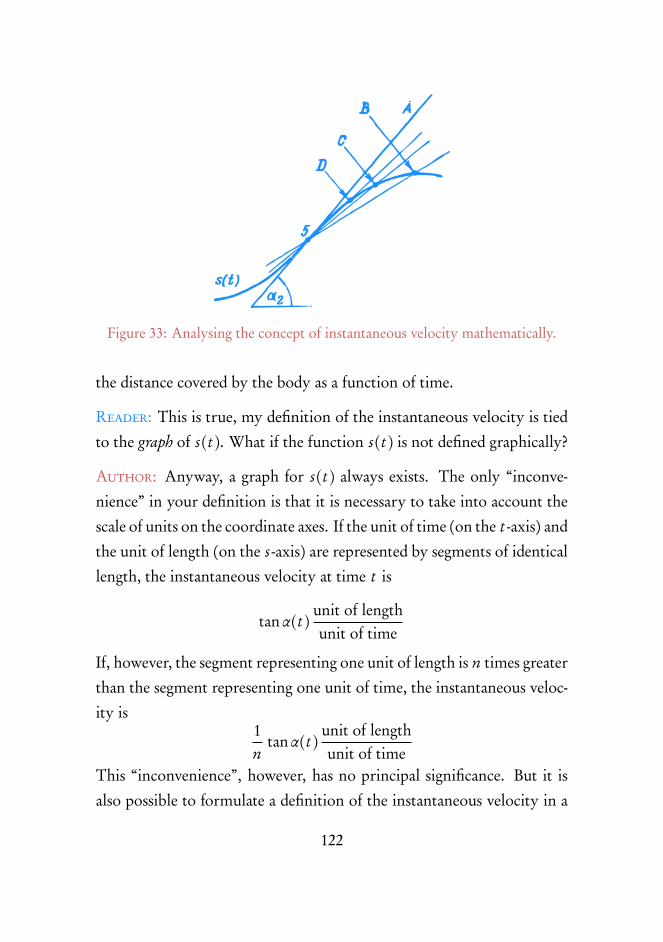
Figure 33: Analysing the concept of instantaneous velocity mathematically.

the distance covered by the body as a function of time.

Reader: This is true, my definition of the instantaneous velocity is tiedto the graph of s(t ). What if the function s(t ) is not defined graphically?

Author: Anyway, a graph for s(t ) always exists. The only “inconve-nience” in your definition is that it is necessary to take into account thescale of units on the coordinate axes. If the unit of time (on the t -axis) andthe unit of length (on the s -axis) are represented by segments of identicallength, the instantaneous velocity at time t is

tanα(t )unit of lengthunit of time

If, however, the segment representing one unit of length is n times greaterthan the segment representing one unit of time, the instantaneous veloc-ity is

1n

tanα(t )unit of lengthunit of time

This “inconvenience”, however, has no principal significance. But it isalso possible to formulate a definition of the instantaneous velocity in a

122

form free of graphic images.

Look at Figure 34 which carries Figure 33 one step further.

Figure 34: Analysing the concept of instantaneous velocity mathematically.

Figure 34 shows that the slope of the secant 5B is a ratio∆s1

∆t1

. In other

words, this is the average velocity for the time interval from t5 to t5+∆t1.

The slope of the secant 5C is∆s2

∆t2

that is, the average velocity for the

time interval from t5 to t5 +∆t2 (∆t2 < ∆t1). The slope of the secant

5D is∆s3

∆t3

that is, the average velocity for the time interval from t5 to

t5 +∆t3 (∆t3 < ∆t2) , etc. Thus, a sequence of the secants convergingto the tangent line (drawn at point 5 of the graph s(t )) corresponds to asequence of the average velocities converging to the slope α2 of the tangentline, that is, to the value of the instantaneous velocity at the timemomentt5.

Reader: It comes out that the instantaneous velocity is the limit of a se-quence of average velocities.

123

Author: Precisely. The instantaneous velocity is in fact the limit of asequence of average velocities, provided that the time interval over whichthe averaging is made tends to zero converging to the moment of time t

(viz., t5 in Figure 34).

Now let us formulate the definition in a more rigorous manner. What wewant to define is the instantaneous velocity of a body at a moment of timet . Consider an arbitrary time interval from t to t +∆t1. The distancecovered by the body during this interval is ∆s1. The average velocity ofthe body during this time interval is

vav(t ,∆t1) =∆s1

∆t1

Next we select a shorter time interval δ t2, from t to t +∆t2, (∆t2 <

∆t1), during which a distance ∆s2 is covered. Consequently, the averagevelocity over ∆t2 is

vav(t ,∆t2) =∆s2

∆t2

We continue this process of selecting shorter and shorter time intervalsstarting at the moment of time t . As a result, we obtain a sequence of theaverage velocities

vav(t ,∆t1), vav(t ,∆t2), vav(t ,∆t3), . . .

The limit of this sequence for∆t → 0 is the instantaneous velocity at themoment of time t :

v(t ) = lim∆t→0

vav(t ,∆t ) (34)

Taking into account that

vav(t ,∆t ) =s(t +∆t )− s(t )

∆t

124

we rewrite expression (35) in the following form

v(t ) = lim∆t→0

s(t +∆t )− s(t )∆t

(35)

As a result, we can formulate the following definition of the instantaneousvelocity.

Definition

The instantaneous velocity at a moment of time t is the limit of asequence of average velocities over time intervals from t to t +∆t

for ∆t → 0.

Reader: Now I realize that instead of talking about a sufficiently small

time interval ∆t (I am referring to our talk about the ratio∆s∆t

at thebeginning of the dialogue), the argument should have been based on thelimit transition for ∆t → 0. In other words, the instantaneous velocity

is not∆s∆t

at a sufficiently small ∆t but lim∆t→0

∆s∆t

Author: Exactly. The definition formulated above for the instantaneousvelocity not only exposes the gist of the concept but gives a rule for itscalculation, provided that an analytical expression for s(t ) is known. Letus make such a calculation assuming that s(t ) is given by expression (33).

Reader: We should substitute (33) for (35). This gives

v(t ) = lim∆t→0

a(t +∆t )2

2− at 2

2∆t

Author: Go ahead. Remove the parentheses.

125

Reader: This will give

v(t ) = lim∆t→0

a(t 2+ 2t∆t +∆t 2− t 2)2∆t

= lim∆t→0

�at +

∆t2

�= at

We have arrived at a familiar formula for the velocity of uniformly accel-erated motion with zero initial velocity:

v(t ) = at (36)

Author: You are absolutely right. I must congratulate you: for the firsttime in your life you have carried the so-called operation of differentia-tion. In other words, you have determined for a given function s(t ) itsderivative, that is, the function v(t ).

Reader: Does it mean that the instantaneous velocity is a derivative?

Author: Note that a derivative exists onlywith respect to a known initialfunction. If the initial function is s(t ) (path as a function of time), thederivative is the instantaneous velocity.

Let us return now to the graph s(t ) shown in Figure 31. Our previous ar-guments and, in particular, relation (36), allow us to transform the graphs(t ) into a graph of the derivative, that is, the function v(t ). A com-parison of the two graphs is given in Figure 35. I recommend that youcarefully analyze Figure 35, interpreting it as a comparison of the graphof a function s(t ) and the graph of its rate of change.

126

Figure 35: Comparing the graph of a function s(t ) and the graph of its rate ofchange.

127

128

Dialogue 9

DERIVATIVE

Author: The previous dialogue gave us an opportunity to introducethe concept of a derivative for a specific example from physics (the in-stantaneous velocity of a body moving non-uniformly along a straightline). Now let us examine this concept from a purely mathematical view-point without assigning any physical meaning to the mathematical sym-bols used.

Figure 36: Examining concept of a derivative on an arbitrary function.

129

Figure 36 shows a graph of an arbitrary function y = f (x). Let us se-lect an arbitrary point x = x0 from the domain of the function. In thesubsequent argument this point is considered as fixed. Now consider an-other point x from the domain of the function and introduce a notation∆x = x − x0. The value ∆x is called the increment of the independentvariable. The increment is considered with respect to the fixed point x0.Depending on the point x, the value of ∆x may. be larger or smaller,positive or negative.

Now let us examine a difference between the values of the function atpoints x = x0+∆x and x = x0:

∆ f (x0) = f (x0+∆x)− f (x0)

The difference∆ f (x0) is said to be the increment of a function f at a pointx0. Since x0 is fixed, ∆ f (x0) should be considered as a function of a vari-able increment ∆x of the independent variable.

Reader: Then it is probably more logical to denote this function by∆ f (∆x), and not by ∆ f (x0), isn’t it?

Author: Probably, you are right. However, the accepted notation is∆ f (x0). Such a notation emphasized the fact that the increment of f (inother words, the given function of ∆x is referred to point x0.

With the concepts of the increment introduced, it is not difficult to eval-uate the rate of change of f close to x0.

Reader: This rate should be described by the ratio∆ f (x0)∆x

. For instance,if we compare ∆ f (x0) with an increment of t at another point from thedomain of the function (say, point x = x1), we may obtain an inequality

∆ f (x1)∆x

>∆ f (x0)∆x

130

and therefore conclude that the rate of change of f close to point x1 isgreater than that close to x0.

Author: Please, be careful. You have not said anything about the vagueincrement∆x. If∆x is too large, the inequality you have just mentionedmay lead to a wrong conclusion. I shall make myself clearer by referringto Figure 37. As you see,

∆ f (x1)∆x

>∆ f (x0)∆x

You must agree, however, that close to point x0 the function changesmuch faster (the graph of the function has a steeper slope) than in thevicinity of x1.

Figure 37: Examining concept of a derivative on an arbitrary function.

Reader: It is necessary that the value of the increment∆x be sufficientlysmall. The smaller is ∆x the more accurate is the information about therate of change of the function close to the point under consideration.

Author: Well, we can do even better than this. We may, for example,

consider the limit of the ratio∆ f (x0)∆x

for ∆x→ 0 (remember the previ-ous dialogue).

131

Reader: This limit will characterize the rate of change of the function f

directly at x = x0.

Author: Exactly. Let us calculate the limit in detail:

lim∆x→0

∆ f (x0)∆x

= lim∆x→0

∆ f (x + x0)− f (x0)∆x

(37)

and examine first of all the mathematical nature of this limit.

Reader: Since point x0 is fixed, it is evidently the limit of the ratio oftwo functions of ∆x for ∆x→ 0 .

Author: Let us denote these functions by F and G:

F (∆x) = f (x0+∆x)− f (x0), G(∆x) =∆x

Reader: Limit (37) is then

lim∆x→0

F (∆x)G(∆x)

where lim∆x→0

F (∆x) = 0 and lim∆x→0

G(∆x) = 0. Hence, we have here a limitsimilar to that discussed at the end of Dialogue Seven, namely, a limit ofthe type

∞∞ .

Author: Right. This limit, that is, the limit of the type∞∞ the main

subject of this dialogue.

The primary requirement in this case is the existence of the limit. It meansthat the function f should be such that

lim∆x→0

F (∆x) = 0

The necessary condition for satisfying this equality is the continuity of f

at x = x0 But we shall discuss this problem later.

132

If the limit of the type∞∞ (in other words, limit (37)) does exist, it is

called “the derivative of the function f at point x = x0 and usually de-noted by f ′(x0).”

Definition

The derivative of a function f at a point x0 (denoted by f ′(x0))is the limit of the ratio of an increment of the function f at thepoint x0 (denoted by∆ f (x0)) to an increment∆x the independentvariable for ∆x→ 0:

f ′(x0) = lim∆x→0

∆ f (x0)∆x

or, in a more detailed notation,

f ′(x0) = lim∆x→0

∆ f (x0)∆x

(38)

Note that you are already familiar with the right-hand side of equation(38) (cf. expression (35) from the previous dialogue).

Reader: Actually the derivative of the function f at point 0 is the limitof the function

FG=

f (x0+∆x)− f (x0)∆x

at ∆x = 0. The independent variable of the functionFG

is the increment∆x.

Author: You are quite right. However, in what follows you must usethe definition of the derivative as formulated above. This definition doesnot involve the function

FG

of ∆x since this function plays, as you un-derstand, only an auxiliary role. We should simply bear in mind that thephrase “the limit of the ratio of an increment∆ f (x0) to an increment∆x

133

for∆x→ 0” describes the limit of a function of∆x, i.e. the functionFG,

which is considered at ∆x = 0.

The derivative can be also interpreted in terms of geometry.

Reader: Shall we do it by using again the tangent to the graph of a func-tion?

Author: Yes, of course. Let us take the graph y = f (x) (Figure 38),fixing a point x = x0. Consider an increment ∆x1 of the argument; thecorresponding increment of the function at point x0 is ∆ f1(x0). Denotethe slope of the chord AB1 by α1 it is readily apparent that

∆ f1(x0)∆x1

= tanα1

Figure 38: Examining concept of a derivative geometrically.

Next take an increment ∆x1 (so that ∆x2 <∆x1). This increment corre-sponds to the increment f2(x0) of the function f at point x0. Denote the

134

slope of the chord AB2 by α2; it is similarly quite apparent that

∆ f2(x0)∆x2

= tanα2

Further, take an increment ∆x3 (so that ∆x3 < ∆x2), and so on. As aresult, we obtain an infinitesimal sequence of increments of the indepen-dent variable:

∆x1,∆x2,∆x3,∆x4, . . .∆xn, . . .

and the corresponding infinitesimal sequence of increments of the func-tion at point x0:

∆ f1(x0),∆ f2(x0),∆ f3(x0),∆ f4(x0), . . .∆ fn(x0), . . .

This leads to a new sequence of the values of the tangent of the slopes ofthe chords AB1,AB2,AB3, . . .ABn, . . .. obtained as a sequence of the ratiosof the two sequences given above

tanα1, tanα2, tanα3, tanα4, . . . tanαn, . . . (39)

Both sequences∆xn and∆ fn(x0) converge to zero. And what can be saidabout the convergence of the sequence (tanαn ) or, in other words, the

sequence∆ fn(x0)∆xn

?

Reader: Obviously, the sequence∆ fn(x0)∆xn

converges to f ′(x0). In other

words, the limit of∆ fn(x0)∆xn

is the derivative of f at x0.

Author: What are the grounds for this conclusion?

Reader: Why, isn’t it self-evident?

Author: Let me help you. Your conclusion is based on Definition 2 ofthe limit of function at a point. Don’t you think so?

135

Reader: Yes, I agree. Indeed, a certain number (in this case f ′(x0 is the

limit of a function Φ(∆x) (in this case Φ =FG) at ∆x = 0 if for any

sequence ∆xn convergent to zero the corresponding sequence (Φ(∆xn))converges to this number. Sequence (39) is precisely the sequence (Φ(∆xn))in our case.

Author: Correct. We have thus found that limn→∞ tanαn = f ′(x0). Now

look at Figure 38 and tell me which direction is the limit for the sequencecomposed of the chords AB1, AB2, AB3, . . .ABn, . . .?

Reader: It is the direction of the tangent to the graph f (x) at point x =x0.

Author: Correct. Denote the slope of the tangent line by α0. Thus

limn→∞ tanαn = tanα0

Consequently,

f ′(x0) = tanα0

We thus obtain the following geometrical interpretation of the derivative:

The derivative of a function f at a point x0 is defined by the slopeof the tangent to the graph of the function f at the point x = x0.

Note that the slope of the tangent is measured relative to the positivedirection of the abscissa axis, so that the derivative of f at point x0 in Fig-ure 39 is positive (at this point tanα0 > 0), while at point x0 the derivativeof f is negative tanα0 < 0).

But the geometrical interpretation of the derivative must not upstage thebasic idea that

136

Figure 39: Examining concept of a derivative geometrically.

The derivative of a function f at a point x0 is the rate of change off at this point.

In the previous dialogue we analyzed the function s(t ) describing thedependence of the distance covered by a body during the time t . In thiscase the derivative of s(t ) at a point t = t0 is the velocity of the body at themoment of time t = t0. If, however, we take v(t ) as the initial function(the instantaneous velocity of a body as a function of time), the derivativeat t = t0 will have the meaning of the acceleration of the body at t = t0.Indeed, acceleration is the rate of change of the velocity of a body.

Reader: Relation (38) seems to allow a very descriptive (if somewhatsimplified) interpretation of the derivative. We may say that

137

The derivative of a function y = f (x) at a point x = x0 shows howmuch steeper the change in y is in comparison with the change inx in the neighbourhood of x = x0.

Author: This interpretation of the derivative is quite justified, and itmay be useful at times.

Getting back to the geometrical interpretation of the derivative, we shouldnote that it immediately leads to the following rather important

Conclusions:

§ The derivative of a function f = const (the derivative of aconstant) is zero at all the points.

§ The derivative of a junction f = ax + b (where a and b areconstants) is constant at all the points and equals a.

§ The derivative of a function f = sin x is zero at the pointsx = +πn (at these points the tangent to the graph of thefunction is horizontal).

This “list” could, of course, be expanded.

Next I would like to attract your attention to the following: from theviewpoint of mathematics a derivative of a function must also be consid-ered as a certain function.

Reader: But the derivative is a limit and, consequently, a number!

Author: Let us clarify this. We have fixed a point x = x0 and obtained

138

for a function f (x) at this point the number

lim∆x→0

∆ f (x0)∆x

For each point x (from the domain of f ) we have, in the general case, itsown number

lim∆x→0

∆ f (x)∆x

This gives a mapping of a certain set of numbers x onto a differ-

ent set of numbers lim∆x→0

∆ f (x)∆x

. The function which representsthis mapping of one numerical set onto another is said to be thederivative and is denoted by f ′(x).

Reader: I see. So far we have considered only one value of the functionf (x), namely, its value at the point x = x0.

Author: I would like to remind you that in the previous dialogue weanalyzed v(t ) which was the derivative of s(t ). The graphs of the twofunctions (i.e. the initial function s(t ) and its derivative v(t )) were evencompared in Figure 35.

Reader: Now it is clear.

Author: I would like to make two remarks with regard to f ′(x).

Note 1. A function f ′(x) is obtained only by using a function f (x).Indeed,

f ′(x) = lim∆x→0

f (x +∆x)− f (x)∆x

(40)

It is as if there is a certain operator (recall Dialogue Four) which generatesf ′(x) at the output in response to f (x) at the input. In other words, thisoperator, applied to the function f (x), “generates” f ′(x). This operator

139

is usually denoted byd

d x. This notation should be interpreted as a single

entity and not as a ratio (it reads: “d over d x”).

Consider an “image”d

d x1 = 2 .

The squares in this expression symbolize the familiar “windows”. “Win-dow” 1 is to input f (x), while “window” 2 outputs f ′(x). Thus,

dd x

f (x) = f ′(x) (41)

Definition:

The operation of obtaining f ′(x) from f (x) is said to be the differ-entiation of f (x).

The operatord

d xperforms this operation over f (x) and is said to be the

operator of differentiation.

Reader: But what exactly isd

d xdoing with f (x)?

Author: It is exactly the operation prescribed by (40). We may say thatd

d x“constructs” the ratio

(x +∆x)− f (x)∆x

from f (x) and determines the limit of this ratio (regarded as a functionof ∆x ) at d x = 0.

Reader: In other words, the operator d x performs a certain limit tran-sition operation, doesn’t it?

140

Author: Certainly. The whole differential calculus (and with it, integralcalculus) can be formulated in terms of certain limit transitions.

Reader: Why should we introduce an operatord

d xif it represents noth-

ing else but the limit transition operation described by (40)?

Author: You have posed a very important question. The problem isthat if we had formulated differential calculus in terms of limits, using therelations of type (40), all books on calculus should have been increasedin their volume several-fold and become hardly readable. The use of therelations of type (41), instead of (40), makes it possible to avoid this.

Reader: But how can we use the relations of type (41) without implicitlyapplying the relations of type (40)?

Author: What is done is this.

First, using (40), we find the result of applying the operatord

d xto a sum,

product, and ratio of functions, and to composite or inverse functionsprovided that the result of applying the operator to the initial function(or functions) is known. In other words, the first step is to establish therules for the differentiation of functions.

Second, using (40), we find out the result of applyingd

d xto some basic

elementary functions (for instance, y = xn, y = sin x, and y = log x ).

After these two steps are completed you can practically forget about therelations of type (40). In order to differentiate a function, it is sufficient toexpress the function via basic elementary functions (the derivatives of whichwere obtained earlier) and apply the rules for differentiation.

Reader: Does it mean that the relations of type (40) could be put asideafter they have been used, first, for compiling a set of differentiation rules

141

and, second, for making a table of derivatives for basic elementary func-tions?

Author: Yes, this is the procedure. Using the differentiation rules andthe table of derivatives for some basic elementary functions you are in aposition to forget about the relations of type (40) and are free to proceedfurther by using the “language” of the relations of type (41). A formalcourse of differential calculus could skip the analysis of limit transitionoperations, that is, the relations of type (40). It is quite sufficient for astudent to learn a set of differentiation rules and a table of derivatives ofsome functions.

Reader: I certainly prefer to be given the foundation.

Author: Our next dialogue will be devoted to a discussion of the pro-gramme of actions as outlined above. At the first step of the programme,the main rules for differentiation will be established on the basis of therelations of (40) and, in addition, the derivatives of three functions y =x2, y = sin x, and y = loga x will be obtained. At the second step, we shallobtain (without reference to the relations of type (40)) the derivatives ofthe following functions:

y = xn, y = x−n, y =p

x, y = cos x, y = tan x, y = cot x, y = arcsin x, y =arccos x, y = arctan x, y = arccot x, and y = ax .

Reader: I’ll be looking forward to the next dialogue. By the way, youwanted to make one more remark about the derivative f ′(x).

Author: Note 2 concerns the natural domain of a derivative. Let a setD be the domain of f (x). The question is whether D is also the domainof f ′(x).

Reader: In any case, the domain of f ′(x) cannot be wider than the do-

142

main of f (x) because in order to find f ′(x) we use f (x).

Author: A carefully balanced answer, to be sure. The domain of f ′(x)is in the general case a subset of D . It is obtained from D as a result of

elimination of those points x for which lim∆x→0

∆ f (x)∆x

does not exist. Bythe way, this subset is called the domain of differentiability of f (x).

Reader: What are the conditions of differentiability of f (x) at any specificpoint x?

Author: Obviously, these conditions are identical to those of the exis-

tence of lim∆x→0

∆ f (x)∆x

at point x. We have already observed that it is the

limit of the type ∞∞ , which necessitates that both the numerator and de-nominator tend to zero. It means that f (x)must be continuous at x. Thefollowing theorem could be proved rigorously.

Theorem:

The continuity of a function f (x) at a point x is a necessary con-dition for the existence of f ′(x) at x.

However, we shall not give the proof of this theorem here. The simplequalitative arguments given above will suffice.

Reader: I wonder whether the continuity of a function is also a sufficientcondition for its differentiability.

Author: No, it is not. Consider, for example, the function y = | log x|. Itis sufficient only to look at its graph (Figure 40) to conclude that at x = 1

the tangent to the graph of the function is, strictly speaking, nonexistent(on approaching x = 1 from the left we have one tangent, viz., the straightline AA, while on approaching x = 1 from the right we have another

143

tangent, viz., the straight line BB ). It means that y = | log x| does nothave a derivative at x = 1, although the function is continuous at thispoint.

Figure 40: Examining the derivative of the function y = | log x|.

In conclusion, let us turn to one interesting property of differentiablefunctions.

Let f (x) be a differentiable function, and its increment∆ f at x be relatedto the increment ∆x of the argument as follows:

∆ f = f ′(x)d x +η(∆x)∆x (42)

where η(∆x)is a function of ∆x.

By dividing both parts of (42) by ∆x, we obtain

∆ f∆x= f ′(x)+η(∆x)

Passing to a limit in both sides of the last equation for∆x gives lim∆x→0

η(∆x) =0.

144

Consequently, η(∆x) is an infinitesimal (we use the same terminology asfor numerical sequences, see Dialogue Three).

Conclusion:

An increment ∆ f of at a point x of a function f (x) differentiableat this point can be represented by two summands, namely, a sum-mand proportional to the increment ∆x of the argument (thissummand is f ′(x)∆x ) and a summand negligible in comparisonwith the first for sufficiently small∆x (this summand is η(∆x)∆x,where η(∆x) is infinitesimal).

Reader: It seems that this is a formulation of the property of “linear-ity on a small scale” that you mentioned in the previous dialogue (seeFigure 32).

Author: Quite true. The main part of the increment of a differentiablefunction (a summand linear with respect to ∆x ) is called the differentialof the function.

145

146

Dialogue 10

DIFFERENTIATION

Author: Now our aim is a practical realization of the programme out-lined in the previous dialogue. This dialogue could be considered as adrill on the calculation of derivatives. We shall divide the talk into threeparts.

1. Differentiation rules.

2. Differentiation of elementary functions y = x2, y = sin x, and y =loga x.

3. Application of differentiation rules to different functions.

Before the start I would like to remind you that the differentiation of afunction f (x) is defined as the operation of obtaining f ′(x) from f (x).

This operation is performed by using the operator of differentiationd

d x

dd x

f (x) = f ′(x)

147

The Differentiation Rules

Author: Rule One. We shall prove the following theorem:

Theorem

The derivative of the sum of two functions equals the sum of theirderivatives provided that they exist, i.e.

dd x[ f (x)+ g (x)] =

dd x

f (x)+d

d xg (x) (43)

Denote f (x)+ g (x) = u(x). Then the theorem can be written as follows:u ′(x) = f ′(x)+ g ′(x). Try to prove this theorem.

Reader: First I write

f ′(x) = lim∆x→0

f (x +∆x)− f (x)∆x

g ′(x) = lim∆x→0

g (x +∆x)− g (x)∆x

u ′(x) = lim∆x→0

u(x +∆x)− u(x)∆x

= lim∆x→0

f (x +∆x)+ g (x +∆x)− f (x)− g (x)∆x

But I don’t know what to do next.

Author: We shall repeat your writing but drop the limit signs:∆u(x)∆x

=f (x +∆x)+ g (x +∆x)− f (x)− g (x)

∆x

=f (x +∆x)− f (x)

∆x+

g (x +∆x)− g (x)∆x

=∆ f (x)∆x

+∆g (x)∆x

148

This gives∆u(x)∆x

=∆ f (x)∆x

+∆g (x)∆x

Reader: I see. Next we use the well-known theorem on the limit of thesum of functions, and the proof is complete.

Author: Quite correct. Rule Two. Let us prove the next theorem:

Theorem

A constant multiplier is factored out of the derivative, that is

dd x[a f (x)] = a

dd x

f (x) (44)

The theorem is immediately proved if we use the following obvious equal-ity

∆ [a f (x)]∆x

= a∆ f (x)∆x

Rule Three. Now we shall consider the theorem on the derivative of theproduct of two functions.

Theorem

The derivative of a function u(x) = f (x) g (x) is calculated by usingthe following formula:

u ′(x) = f ′(x) g (x)+ f (x) g ′(x) (45)

provided that the derivatives f ′(x) and g ′(x) exist.

Formula (45) is called the Leibnitz formula. Another expression for thesame formula is:

dd x( f g ) = g

dd x

f + fd

d xg

149

Reader: Apparently, as in the proof of the first theorem, wemust express∆u(x)∆x

through∆ f (x)∆x

and∆g (x)∆x

. But how to do it?

Author: The simplest way is

u +∆u = ( f +∆ f )(g +∆g )

= f g + g∆ f + f ∆g +∆ f ∆g

Hence,∆u = g∆ f + f ∆g +∆ f ∆g

consequently,

∆u(x)∆x

= g (x)∆ f (x)∆x

+ f (x)∆g (x)∆x

+∆ f (x)∆x

∆g (x)

Now we find the limit for ∆x → 0. Notice that neither g (x) nor f (x)depends on ∆x, and ∆g (x) tends to zero. As a result,

lim∆x→0

∆u(x)∆x

= lim∆x→0

g (x)∆ f (x)∆x

+ lim∆x→0

f (x)∆g (x)∆x

The theorem is thus proved.

Rule Four. The next theorem is related to the derivative of the ratio oftwo functions.

Theorem

The derivative of a function u(x) =f (xg (x)

is:

u ′(x) =f ′(x)g (x)− f (x)g ′(x)

g 2(x)(46)

provided that the derivatives f ′(x) and g ′(x) exist, and that g (x) ̸=0.

150

It can be written in a different form:

dd x

�fg

�=

gd

d xf − f

dd x

g

g 2

Try to prove this theorem.

Reader: I shall proceed by analogy with the preceding proof. I can writeHence,

∆u =f +∆ fg +∆g

− fg

=g∆ f∆x− f∆g∆x

g 2+ g∆g

This yields,

∆u∆x=

g∆ f∆x− f∆g∆x

g 2+ g∆g

Passing then to the limit for ∆x → 0, I take into account that neither g

nor f depend on ∆x, and that ∆g also tends to zero. Using the knowntheorems on the limit of the product and the sum of functions, we obtain

lim∆x→0

∆u∆x= lim∆x→0

�1

g 2+ g∆g

�lim∆x→0

�g∆ f∆x− f∆g∆x

�=

1g 2

�g lim∆x→0

∆ f∆x− f lim

∆x→0

∆g∆x

�This completes the proof.

Author: Very good. Now we shall discuss the, problem of the differ-entiation of a composite function (for composite functions, see DialogueFive. Let w = h(x) be a composite function, and h(x) = g [ f (x)]. This

151

composite function is the composition of two functions w = g (y) andy = f (x).

I remind you that the derivative f ′(x) indicates how faster y chargescompared to x and the derivative g ′(y) indicates how faster w changescompared to y. Consequently, the product g ′(y) f ′(x)must indicate howfaster w changes compared to x, i.e. it equals the derivative h ′(x).

Rule Five. Thus we arrive at the differentiation rule for composite func-tions.

Theorem

The derivative of a composite function h(x) = g [ f (x)] is:

h ′(x) = g ′(y) f ′(x) (47)

Reader: We have arrived at this rule using very simple arguments. Iwonder whether they can be regarded as a proof of the rule.

Author: No, of course not. Therefore I am going to give the proof ofthe differentiation rule for composite functions.

Let the independent variable x have an increment ∆x such that x +∆x

belongs to the domain of f (x). Then the variable y will have an incre-ment∆y = f (x+∆x)− f (x), while the variable w will have an increment∆w = g (y+∆y)− g (y). Since the derivative g ′(y) exists. the increment∆w can be expressed as follows

∆w = g ′(y)∆y +η∆y

where η→ 0 for∆y→ 0 (see expression (6) from the previous dialogue).

152

Dividing both sides of the equation by ∆x, we obtain

∆w∆x= g ′(y)

∆y∆x+η∆y∆x

Next we pass to the limit for ∆x→ 0

lim∆x→0

∆w∆x= g ′(y) lim

∆x→0

∆y∆x+ lim∆x→0

�η∆y∆x

�Since lim

∆x→0

∆w∆x = h ′(x) and lim

∆x→0

∆y∆x = f ′(x), we have

h ′(x) = g ′(y) f ′(x)+ f ′(x) lim∆x→0

η

And since ∆y→ 0 for ∆x→ 0,

lim∆x→0

η= lim∆y→0

η= 0

Hence we arrive at (48), namely, at the rule for the differentiation ofcomposite functions.

Rule Six. Finally, I shall give (without proof) the rule for the differenti-ation of inverse functions.

Theorem

If a derivative y ′(x) of an initial monotonic function y(x) exists andis not equal to zero, the derivative of the inverse junction x(y) iscalculated by the formula:

x ′(y) = 1y ′(x)

(48)

Reader: It seems that this formula can be easily obtained if we make useof the geometrical interpretation of the derivative. Really, consider thegraph of a monotonic function y(x) (Figure 41); its derivative at point

153

x0 is tanα. The same curve can, obviously, be regarded as the graph ofthe inverse function x(y), with y considered as the independent variableinstead of x, and x considered as the dependent variable instead of y. Butthe derivative of the inverse function at point y0 is tanβ (see the figure).Since α+β=

π

2we have

Figure 41: Derivative of a function and its inverse.

tanβ=1

tanα

This gives the above-cited differentiation rule for inverse functions.

Author: I must admit that although your line of reasoning is not a rig-orous mathematical proof, it is an example of an effective application ofgeometrical concepts.

154

The Differentiation of Functions

y = x2, y = sin x, and y = loga x

Author: Using (40) from the previous dialogue, calculate the derivativesof the three indicated functions. Start with y = x2. Go ahead.

Reader: I write

y +∆y = (x +∆x)2 = x2+ 2x∆x +∆x2

Hence,

∆y = 2x∆x +∆x2

Consequently,∆y∆x= 2x +∆x

Further we pass to the limit for ∆x→ 0

lim∆x→0

∆y(x)∆x

= 2x

Therefore,

y ′(x) = 2x

Author: You have thus obtained the result of applying the operatord

d xto the function y = x2:

dd x

x2 = 2x (49)

We observe that for a quadratic function y = x2 at the input of the oper-

atord

d xwe obtain a linear function y = 2x at the output.

Now try to differentiate the function y = sin x.

155

Reader: I shall write

y +∆y = sin(x +∆x)2 = sin x cos∆x + cos x sin∆x

Hence,∆y = sin x cos∆x + cos x sin∆x − sin x

Author: You had better use here the formula for the difference betweentwo sines, not the formula for the sine of the sum. Represent ∆y in theform

∆y = sin(x +∆x)− sin x = 2sin∆x2

cos�

x +∆x2

�Next we obtain

∆x∆y=

sin ∆x2

∆x2

cos�

x +∆x2

�In taking the limit for∆x→ 0, recall a result obtained in Dialogue Seven:

lim∆x→0

sin∆x∆x

= 1

Reader: Yes, I see. Therefore,

lim∆x→0

∆x∆y= lim∆x→0

sin ∆x2

∆x2

lim∆x→0

cos�

x +∆x2

�= lim∆x→0

cos�

x +∆x2

�= cos x

Author: The operatord

d xapplied to the function y = sin x thus gener-

ates the function y = cos x:

dd x

sin x = cos x (50)

156

Now we have to differentiate the function y = loga x. This time, how-ever, we should start with a discussion of the transcendental number e

(which is usually called the “base of natural or Napierian logarithms”).The number e may be defined as the limit of a numerical sequence

e = limn→∞

�1+

1n

�n(51)

The approximate value of e is: e = 2.7182818284590 . . . Using (51), we

can show that e is also the limit of y = (1+ x)1x for x tending to zero

e = limx→0(1+ x)

1x (52)

We shall omit the proof of (52).

Reader: It seems that (52) follows logically from (51).

Author: Far from it. Don’t forget that in (51) we deal with the limitof a numerical sequence, while in (52) with the limit of a function at apoint. While n are integers, x belongs to the real line (with the exceptionof x = 0). Therefore, the transition from (51) to (52) requires a good dealof time and space.

Now turn to the differentiation of y = loga x. Follow the line adoptedabove.

Start.

Reader: Obviously,

y +∆y = o ga(x +∆x)

Hence,

∆y = loga(x +∆x)− loga x

157

= logax +∆x∆x

and, consequently,∆x∆y=

1∆x

logax +∆x

x

At this point I would have to find the limit for ∆x→ 0.

Author: I shall give you a hand here. We can rewrite

∆x∆y= loga

� x +∆xx

� 1∆x

= loga

�1+∆xx

� x∆x· 1x

=1x

loga

�1+∆xx

� x∆x

Reader: I see. This gives

∆x∆y=

1x

loga

�1+∆xx

� x∆x

To find the limit for ∆x→ 0, we use (52). As a result

lim∆x→0

∆x∆y=

1x

lim∆x→0

loga

� x +∆xx

� x∆x

=1x

loga e

=1x· 1lna

(symbol ln is the standard notation for the natural logarithm).

158

Author: We have thus found that the operatord

d xapplied to the func-

tion y = loga x gives y =1x· 1lna

:

dd x

loga x =1x· 1lna

(53)

Notice that the natural domain of the function y =1x· 1lna

in (53) ]0,∞[.We can sum up our conclusions now.

Using relation (40) from Dialogue Nine, first, we have established thesix differentiation rules and, second, we have differentiated three func-tions. The results are summarized in Table on the next page, and Fig-

ure 42 graphically represents the result of the action of the operatord

d xon the three selected functions. The left-hand column in the figure liststhe graphs of the three functions f (x), and the right-hand column showsthe graphs of the corresponding derivatives f ′(x).

In what follows we shall not use formulas of type (40) from DialogueNine, that is, we shall not operate in terms of limit transitions. Usingthe results obtained above, we shall find the derivatives for a number ofelementary functions without calculating the relevant limits.

159

The Differentiation Rules

Rule 1: the differentiation ofthe sum of functions

dd x( f + g ) =

dd x

f +d

d xg

Rule 2: the differentiationof the function with constantterm

dd x(a f ) = a

dd x

f (a = constant)

Rule 3: the differentiation ofthe product of functions

dd x( f g ) = f

dd x

g + gd

d xf

Rule 4: the differentiation ofthe ratio of functions

dd x

fg=

gd

d xf − f

dd x

g

g 2

Rule 5: the differentiation ofcomposite functions

dd x

g [ f (x)] =�

dd f

g ( f )�

dd x

f (x)

Rule 6: the differentiation ofinverse functions

dd y

x(y) =1

dd x

y(x)

160

Figure 42: Graphs of some basic functions and their derivatives.

161

The Application of the Differentiation Rules to

Different Functions

Author: As a first example, consider the function y = xn. Prove thatdifferentiation gives y = nxn−1 , that is,

dd x

xn = nxn−1 (54)

Prove this proposition by using the method of mathematical induction.

Reader: For n = 2 formula (54) holds and yields (49). Assume now that(54) holds for n = m. We have to prove that it is also true for n = m+1.We write x m+1 = x m x and use the Leibnitz formula (Rule Three):

dd x(x m x) = x

dd x

x m + x m dd x

x

Sinced

d xx = 1 and according to the assumption

dd x

x m = mx m−1, weobtain

dd x

x m+1 = mx x m−1+ x m = (m+ 1)x m

The proof is completed.

Author: The next example is the function y = x−n. Differentiate thisfunction using Rule Four and (54).

Reader: This is simple. Applying Rule Four, we obtain

dd x

�1xn

�=− d

d xxn

x2n

By virtue of (54),d

d xx−n =−nx−(n+1) (55)

162

Author: One particular result that follows from (57) is

dd x

�1x

�=− 1

x2 (56)

The next example is the function y =p

x.

Reader: Here I shall use Rule Six (the differentiation rule for inversefunctions). The inverse function involved is x = y2. Its derivative isgiven by (49). As a result,

dd xp

x =1

dd x

y2

=1

2y=

12p

x

Thusd

d xp

x =1

2p

x (57)

Author: Now we can pass to the trigonometric functions. Consider thefunction y = cos x.

Reader: I propose to use (58) and the identity sin2 x + cos2 = 1. Bydifferentiating both sides of the identity and using Rule One, we obtain

dd x

sin2 x +d

d xcos2 x = 0

Next, by applyingRule Five (the differentiation rule for composite func-tions) in conjunction with (49), we find

2sin xd

d xsin x + 2cos x

dd x

cos x = 0

From (58),d

d xsin x = cos x so that

dd x

cos x =− sin x

163

Author: That is correct, although the result can be obtained in a simplerway. Better use the identity cos x = sin

�π2− x�. Further, applying Rule

Five, we obtain

dd x

sin�π

2− x�=�

dd y

sin y�

dd x

�π2− x�

(here y =π

2− x )

Making use of (58), we find

dd x

sin�π

2− x�=− d

d ysin y =−cos y =− sin x

Using now the suggested identity, we arrive at the final result:

dd x

sin x =−cos x (58)

Reader: The operation of differentiation thus “turns” the sine into thecosine and, vice versa, that is, the cosine in to the sine.

Figure 43: Graphs of the sine and cosine functions.

Author: . Yes, it does. But in the last case the sign changes too, that is,the cosine is transformed into the sine with a negative sign. If you plot thegraphs of sin x and cos x in the same system of coordinates (Figure 43),

164

you will find that at points x where one of the functions reaches maxi-mum or minimum (takes the value 1 or -1) the other function vanishes.It is readily apparent that this fact has direct relation to your remark. If,for example, at a certain point x the function sin x assumes its maximumvalue, the tangent to its graph at the same point will, obviously, be hori-zontal.

Consequently, the derivative of the function (i.e, cos x ) must vanish atthis point. I recommend that you carefully analyze Figure 43. In par-ticular, follow the correspondence between the slope of the tangent tothe graph of the function drawn at different points and the sign of thederivative at the same points.

Now turn to the next example, the function y = tan x. Difierentiatethis function using the results of the differentiation of sin x and cos x andapplying Rule Four.

Reader: This will be easy:

dd x

�sin xcos x

�=

cos xd

d xsin x − sin x

dd x

cos x

cos2 x

=cos2 x + sin2 x

cos2 x

=1

cos2 xFinally,

dd x

tan x =1

cos2 x(59)

Author: The result for y = cot x can be obtained similarly:

dd x

cot x =− 1sin2 x

(60)

165

In order to differentiate y = arcsin x, we use Rule Six

dd x

arcsin x =1

dd y

sin y

=1

cos y

=1

cos (arcsin x)

Sincecos (arcsin x) =p

1− x2

we obtaind

d xarcsin x =

1p1− x2 (61)

In order to differentiate y = arccos x, it is sufficient to use (60) and theidentity

arcsin x + arccos x =π

2Therefore,

dd x

arccos x =− 1p1− x2 (62)

Using Rule Six, we differentiate the function y = arctan x

dd x

arctan x =1

dd y

tan y

= cos2 y

= [cos (arctan x)]2

Sincecos (arccos x) =

1p1+ x2

166

we obtaind

d xarctan x =

1p1+ x2 (63)

And, finally, the differentiation of y = arccot x is carried out by using theidentity

arctan x + arccot x =π

2and yields

dd x

arccot x =− 1p1+ x2 (64)

We have thus performed the differentiation of all elementary trigonomet-ric and inverse trigonometric functions,

In conclusion, let us examine the exponential function y = ax . Using(53) and Rule Six, we obtain

This gives

dd x

ax = ax lna (65)

Result (65) is very interesting. We see that the differentiation of the ex-ponential function y = ax again yields the exponential function ax mul-tiplied by the constant term lna. In a particular case of a = e , we haveln e = 1,and therefore

dd x

e x = e x (66)

The exponential function y = e x is simply called the exponential curve.From (66) it follows that differentiation transforms this function into it-self.

167

168

Dialogue 11

ANTIDERIVATIVE

Reader: Differentiation is an operation of finding a function f ′(x) for agiven function f (x). Presumably, an inverse operation is possible as well,isn’t it?

Author: An inverse operation indeed exists. It is called integration. In-tegration of a function f (x) is an operation by which the so-called anti-derivative is found for the given function f (x).

Definition

An antiderivative is defined as a function F (x) whose derivativeequals an initial function f (x):

f (x) =d

d xF (x) (67)

Reader: Quite clear. In the preceding dialogue we were seeking a deriva-tive f ′(x) for a given function f (x), and now we deal with a situation inwhich the given function f (x) is the derivative of a yet unknown function

169

F (x).

Author: Absolutely right. Take, for example, a function f (x) = 2x2−3x. The differentiation of this function gives its derivative

f ′(x) = 4x − 3

and its integration gives the antiderivative

F (x) =23

x3− 32

x2

Reader: But how did you find this antiderivative?

Author: This was simple. I resorted to the well-known rules of differ-entiation but in a reverse order. In other words, I mentally searched for afunction that would yield our function f (x) = 2x2− 3x after differentia-tion. You can easily verify that

F ′(x) = 23

3x2− 32

2x = 2x2− 3x

Reader: But then why not take as this antiderivative, for example, a

function F (x) =23

x3− 32

x2+ 2. It will again yield F ′(x) = 2x2− 3x.

Author: You noticed a very important feature. Indeed, an antideriva-tive found for a given function is not unique. If F (x) is an antiderivative(for a function f ), then any function F (x) +C , where C is an arbitraryconstant, is also an antiderivative for the initial function because

dd x[F (x)+C ] =

dd x

F (x)+d

d xC =

dd x

F (x)

Reader: This means, therefore, that each given function f (x) corre-sponds to a family of antiderivatives, F (x)+C doesn’t it?

170

Author: Precisely. Take a graph of one of the anti-derivatives. By trans-lating it along the y-axis, you will obtain a family of the curves of an-tiderivatives for a given function f . For example, let f (x) = sin x, Thecurves of antiderivatives for this function are plotted in Figure 44. Thesecurves plot functions

F (x) =−cos x +C

(the dash curve is the graph of the function f (x) = sin x ) . The constantsC were taken with an increment of 0.5. By reducing this increment, onecan obviously obtain a pattern of arbitrarily high density of F (x) curves.

Figure 44: Graphs of the anti-derivatives of the function f (x) = sin x.

The figure clearly shows that all the antiderivatives belong to one family(in other words, correspond to the same initial function f ). This maynot always be as clear if the function is represented in an analytical form.Take, for example, functions F1 =−cos x and F2 = 3−2cos2 x

2. It would

be difficult to say at the first glance that these two functions are the an-tiderivatives of one and the same function (namely, f = sin x ). However,

171

since 2cos2 x2= 1+ cos x, we find

F2(x) = 3− 1− cos x =−cos x + 2

Reader: I guess it would be possible to find directly that F ′1(x) = F ′2(x),wouldn’t it?

Author: Of course, it would:

dd x

F2(x) =−2d

d xcos2 x

2= 4cos

x2

sinx2· 1

2= sin x

dd x

F1(x) =d

d x(−cos x) = sin x

But the easiest way is to notice that F2− F1 =C .

We could find numerous such examples. For instance, it is not difficultto check that the following pairs of functions belong to the same familyof antiderivatives (each pair to its own family):

(a) F1 = x2− 2x + 3, F2 = (x − 1)2

(b) F1 = arcsin x, F2 = 1− arccos x

(c) F1 = tan x sin x + cos x, F2 = (2cos x + 1)1

cos x

Thus, in case (a) we find F2− F1 =−2; both functions are the antideriva-tives of the function f = 2x − 2.

Please, check cases (b) and (c) yourself.

Reader: In case (b) F2 − F1 = (1− arccos x ++arcsin x) = 1− π2

both

functions are the antiderivatives of the function f =1

1− x2

172

Case (c) ismore intricate. Some preliminarymanipulations are necessary:

F1(x) = tan x sin x + cos x =sin2 x + cos2 x

cos x=

1cos x

F2(x) =2cos x + 1

cos x= 2+

1cos x

Therefore, F2− F1 = 2. Both functions (F1 and F2) are the antiderivatives

of f =sin xcos2 x

Author: Correct. Now, taking into account the results obtained in theprevious dialogue, we can compile a table (see Table 2) which gives vari-ous functions f (x) in the first column the corresponding derivatives f ′(x)in the second column, and the antiderivatives F (x) +C , correspondingto the functions f (x), in the third column. I want to stress once more:the transformation f (x)→ f ′(x) is the operation of differentiation of thefunction f (x), and the transformation f (x)→ [F (x)+C ] is the operationof integration of the function f (x).

173

A List of Derivatives and Antiderivatives for Selected Functions

Function Derivative Antiderivativef (x) f ′(x) F(x)

1 a 0 ax +C

2 xn nxn−1 1n+ 1

xn+1+C

3 e x e x e x +C

41x

− 1x2

ln x +C

5p

x1

2p

x23

xp

x +C

6 sin x cos x −cos x +C

7 cos x − sin x sin x +C

81

cos2x 2

sin xcos3 x

−cot x +C

91

sin2 x−2

cos xsin3 x

tan x +C

101

1+ x2− 2x(1+ x2)2

arctan x +C

174

Reader: Examples 8 , 9 , and 10 in Table 2 give an impression thatthe transformation f (x)→ f ′(x) is more complicated than the transfor-mation f (x)→ [F (x)+C ].

Author: This impression stems from a special selection of the functionsf (x). Thus, it is easier to differentiate the function tan x than the function

1cos2 x

. Indeed, in the latter case we have to use the rules for differentia-tion of a ratio of two functions or of a composite function.

In general, it should be noted that the operation of integration is substan-tially more complicated than that of differentiation. The differentiationof elementary functions invariably gives elementary functions. By em-ploying the rules for differentiation discussed in the previous dialogue,you will be able (and with no difficulties, as a rule) to differentiate practi-cally any elementary function. But integration is quite a different propo-sition. The rules for the integration of elementary functions comprisenumerous techniques, and wewould need several special dialogues to scanthem. But the main point is that not every elementary function has an el-ementary function for its antiderivative. As one example, I shall mention

the antiderivatives of such elementary functions as1

log xor

1p1+ x2

. As

a rule, in such cases one is forced to resort to the methods of the so-callednumerical integration.

Reader: I was very attentive andwant to pose two questions. First: Whatis meant by the term elementary function?

Author: In Dialogue Nine I gave examples of the so-called fundamen-tal elementary functions (xn, x−n, x1/n, sin x, cos x, tan x, cot x, arcsin x,

arccos x, arctan x, arccot x, ax , loga x ]. An elementary function is any func-tion which can be formed of fundamental elementary functions by a finite

175

number of the operations of addition, subtraction, multiplication, divi-sion, involution, evolution, and taking a modulus, as well as by using therules for obtaining inverse and composite functions. All the functionsused in the previous dialogues are elementary (with an exception of theDirichlet function mentioned in Dialogue Five), and many of them arefundamental elementary functions.

Reader: My second question concerns the rules for integration you referto. Could you give at least some examples?

Author: I shall quote three simplest rules.

Three Simple Rules for Integration

1 If F is an antiderivative for f . and G is an anti-derivative forg , an antiderivative for the sum of the functions f + g is afunction F +G.

2 If F is an antiderivative for f an antiderivative for a functiona f , where a is a constant, is a function aF .

3 If F (x) is an antiderivative for f (x), and a and b are con-stants, an antiderivative for a function f (ax+b ) is a function1a

F (ax + b ).

All the three rules are proved readily by using the rules for differentia-tion (in the third rule one has to apply the rule for the differentiation ofcomposite functions). Indeed,

1d

d x(F +G) =

dd x

F +d

d xG = f + g

176

2d

d x(aF ) = a

dd x

F = a f

3d

d x

�1a

F (ax + b )�=

1a

dd x

F (ax + b ) =1a

dd y

F (y)d

d x(ax + b )

=1a

f (y)a = f (y) = f (ax + b )

here: y = ax + b

Of course, the three rules cited above do not exhaust a rich collection ofintegration rules available in calculus.

But here these three rules will be sufficient since our goal is quite modest:to give the fundamental idea of an anti-derivative.

Reader: Our discussion of a derivative covered its geometrical interpre-tation as well. Is there a geometrical interpretation of an antiderivative?

Author: Yes, there is. Let us find it (besides, we shall need it later).

Consider a function f (x). For the sake of simplicity, assume that thisfunction is monotonic (and even increasing). Later we shall drop themonotonicity of a function. The most important is that the functionbe continuous over the chosen interval (i.e. over the interval on which itis defined). Figure 45 shows a shaded area (the so-called curvilinear trape-zoid) bounded by the graph of the function f (x), the interval [a, x] of thex-axis, and two perpendiculars erected from points a and x on the x-axis.Let point a be fixed; as for point x (the right-hand end of the interval[a, x]), it is not fixed and can assume values from a upward (within thedomain of definition of the function). Obviously, the area of the curvi-linear trapezoid shaded in the figure is a function of x. We shall denote itby S(x),

Now turn to Figure 46. Let us give an increment ∆x to the independent

177

Figure 45: Examining the geometrical interpretation of the antiderivative.

variable x. The interval [a, x +∆x] corresponds to the area S(x +∆x).Denote ∆S(x) = S(x +∆x)− S(x). The increment ∆S(x) is, obviously,the area of the shaded curvilinear trapezoid. The figure shows that

area ADEF <∆S(x)< area ABC F

But the area ADEF is equal to f (x)∆x, and the area ABC F is equal tof (x +∆x)∆x. Therefore,

area ADEF <∆S(x)< area ABC F

orf (x)∆x <

∆S(x)∆x

< f (x +∆x)

or0<�∆S(x)∆x− f (x)�< [ f (x)+∆x)− f (x)] =∆ f (x)

Now we find the limiting values of these inequalities for ∆x tending tozero. By virtue of the continuity of the function f (x) we conclude that

178

Figure 46: Examining the geometrical interpretation of the antiderivative.

lim∆x→0

∆ f (x) = 0. Consequently,

lim∆x→0

�∆S(x)∆x− f (x)�= 0

As the function f (x) is independent of ∆x, the last relation yields

lim∆x→0

∆S(x)∆x

= f (x) (68)

By the definition of derivative,

lim∆x→0

∆S(x)∆x

= S ′(x)

Consequently, relation (68) signifies that

f (x) = S ′(x) (69)

Thus, in terms of geometry, the antiderivative of the function f , takenat point x , is the area of curvilinear trapezoid bounded by the graph of thefunction f (x) over the interval [a, x] of the x -axis.

179

Reader: Presumably, it is one of the possible anti-derivatives, isn’t it?

Author: Definitely.

Reader: But it is evident that the area S(x) also depends on the choice ofpoint a.

Author: Absolutely correct. By choosing different points a, we shallhave different areas of curvilinear trapezoids and, correspondingly, dif-ferent antiderivatives. But all of them will be the antiderivatives of thefunction f taken at point x. It is only important that in all cases a < x.

Reader: Then why is it that point a vanishes from the final results?

Author: Your bewilderment is understandable. Let us reformulate theresults obtained above. Let F (x) be an antiderivative of a function f (x)taken at point x. According to (69), we can write

S(x) = F (x)+C

(here we have used the following theorem: if two functions have equalderivatives, the functions will differ by a constant term). The constant C

is found readily since S(a) = 0. Therefore,

S(a) = F (a)+C = 0

Hence, C =−F (a). This gives

S(x) = F (x)− F (a) (70)

Conclusion

If F (x) is an antiderivative of a function f (x), then the area S(x) ofa curvilinear trapezoid bounded by the graph of the junction f (x)

180

over the interval [a, x] is given by the difference F (x)− F (a).

You see now that point a is introduced explicitly.

Reader: Now everything is clear,

Author: Relation (69) (and from it, (70)) can be obtained for everycontinuous function; the monotonicity of a function is not a necessarycondition. Consider a function f (x)whose graph is plotted in Figure 47.We choose a point x and wish to prove that for any ϵ > 0 there is δ > 0

such that ����∆S(x)∆x− f (x)����< ϵ (71)

for all ∆x satisfying the condition |∆x|<δ.

Figure 47: Examining the geometrical interpretation of the antiderivative.

Reader: Shall we consider point x as fixed?

Author: Yes. Increments ∆x and, correspondingly, ∆S(x), are always

181

considered for a definite point x. So we take an arbitrary number ϵ > 0

(shown in the figure). As f (x) is a continuous function, there is a numberδ > 0 such that

| f (x)+∆x − f (x)|< ϵ (72)

for all ∆x satisfying the condition |∆x| < 0. This number δ is the onewe were to find.

Indeed, let us choose, for definiteness, that∆x > 0 but specify that∆x <

δ. The area of the curvilinear trapezoid shaded in Figure 47 will be de-noted by ∆S(x) (this trapezoid is bounded by the graph of the functionf (x) over the interval [x, x+∆x]. Inequality (72) yields (see the figure):

[ f (x)− ϵ]∆x <∆S(x)< [ f (x)− ϵ]∆x

or[ f (x)− ϵ]< ∆S(x)

∆x< [ f (x)− ϵ]

or,

−ϵ <�∆S(x)∆x− f (x)�< ϵ

or, finally. ����∆S(x)∆x− f (x)����< ϵ

which is what we wanted to prove.

You see that a function f needn’t be monotonic: relation (69) (and withit, (70) is easily generalized to the case of an arbitrary continuous functionf .

Now let us turn again to Figure 44 that gives a family of graphs of theantiderivative F (x) =−cos x +C for the function f (x) = sin x. Indicatewhich of these graphs (which antiderivative) stands for S(x) in each ofthe following three cases: (a) a = 0, (b) a =

π

2, and (c) a =π.

182

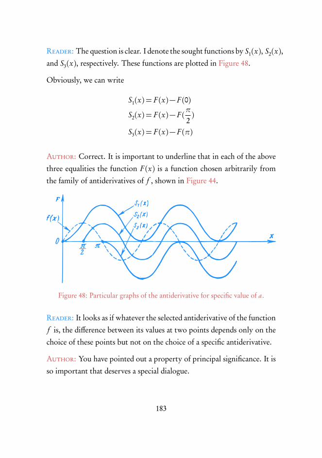
Reader: The question is clear. I denote the sought functions by S1(x), S2(x),and S3(x), respectively. These functions are plotted in Figure 48.

Obviously, we can write

S1(x) = F (x)− F (0)

S2(x) = F (x)− F (π

2)

S3(x) = F (x)− F (π)

Author: Correct. It is important to underline that in each of the abovethree equalities the function F (x) is a function chosen arbitrarily fromthe family of antiderivatives of f , shown in Figure 44.

Figure 48: Particular graphs of the antiderivative for specific value of a.

Reader: It looks as if whatever the selected antiderivative of the functionf is, the difference between its values at two points depends only on thechoice of these points but not on the choice of a specific antiderivative.

Author: You have pointed out a property of principal significance. It isso important that deserves a special dialogue.

183

184

Dialogue 12

INTEGRAL

Author: We know already that the difference between the values of anantiderivative at two arbitrary points depends only on the choice of thesepoints (and, evidently, on the type of the initial function f (x)). As thesetwo points we choose points a and b , that is, consider an increment of anantiderivative, F (b )− F (a), This increment plays a very important roleamong the tools of calculus; it is called the integral.

Definition

The increment of an anti-derivative F of a function f , i,e. F (b )−F (a), is said to be the integral of f from a to b .

The notation of the integral is:∫ ba

f (x)d x

(it reads: “integral of f of x, d x, from a to b”). The numbers a and b

are the lower and upper limits of integration. The function f is said to beintegrand, and x the integration variable.

185

Consequently, if F is one of the antiderivatives of the function f , thenthe definition of an integral states that∫ b

af (x)d x = F (b )− F (a) (73)

Formula (73) is known in the literature on mathematics as the Newton-Leibnitz formula. Remember that F here is an arbitrary antiderivative ofthe function f .

Figure 49: Examining the geometrical interpretation of the integral as area.

Reader: As far as I understand, the integral of the function f from a tob is precisely the area of the curvilinear trapezoid bounded by the graphof the function f (x) over the interval [a, b ]. Is that right?

Author: Absolutely. The expression∫ ba

f (x)d x

is nothing less than the area of this geometrical figure. Figure 49 showsthree cases plotting different integrands: (a) f (x) = 2x, (b) f (x) = x2,(c) f (x) =

px.

186

The limits of integration are chosen identical in all the three cases: a =1, b = 2. The corresponding areas of the curvilinear trapezoids are shadedin the figure:

S1 =∫ 2

12x d x

S2 =∫ 2

1x2 d x

S3 =∫ 2

1

px d x

The numbers S1, S2, and S3 are different because the integrands f (x) aredifferent.

We thus find that the expression∫ ba

f (x)d x

works as a functional (recall Dialogue Four). You “input” in it a functionf , and it “outputs” a number S.

By the way, you can easily find how this functional works. To achievethis, use formula (73) and take into account that the antiderivative of the

function f (x) = 2x is F (x) = x2+C , that of f (x) = x2 is F (x) =13

x3+C ,

and that of f (x) =p

x is F (x) =23

xp

x +C .

The standard notation is: F (b )− F (a) = F (x)|ba . Therefore,∫ 21

2x d x = x2|21 = 4− 1= 3∫ 21

x2 d x =13

x3|21 = 13(8− 1) =

73∫ 2

1

px d x =

23

xp

x|21 = 23(2p

2− 1)

187

With the function 2x at the “input” of the functional∫ 2

1f (x)d x, we ob-

tain at the “output” the number 3; with x2 at the “input”, we obtain at

the “output” the number73; and with

px at the “input”, we obtain at the

“output” the number23(2p

2− 1).

Reader: I see that we can rather easily find the areas of various curvilineartrapezoids!

Author: More than only curvilinear trapezoids. For instance, try tofind the area of the figure shaded in Figure 50.

Figure 50: Curvilinear trapezoids as integral of a function.

Reader: This area is the difference between the areas of two curvilineartrapezoids:

S =∫ 1

0

px d x −∫ 1

0x2 d x

Therefore,

S =23

xp

x|10− 13

x3|10 = 23− 1

3=

13

Author: Correct. Consider another example. Find the area of theshaded figure in Figure 51.

188

Figure 51: Curvilinear trapezoid as the integral of a function.

Reader: The graphs of the functions sin x and cos x intersect at the pointx =

π

4. Consequently, one has to use the antiderivative of the function

sin x over the intervalh0,π

4

iand that of the function cos x over the in-

tervalhπ

4,π

2

i. Hence,

S =∫ π

4

0sin x d x +∫ π

2

π4

cos x d x =−cos x|π40 + sin x|π2π4

=−�cosπ

4− cos0�+�sinπ

2− sin

π

4

�=−�p

22− 1

�+�

1−p

22

�= 2−p2

Author: Perfectly right. Now we shall discuss one “fine point”, return-ing to formula (73) and rewriting it in the form∫ x

af (t )d t = F (x)− F (a) (74)

What has been changed by this rewriting?

189

Reader: First, we have replaced the constant upper limit of integration(the number b ) by the variable limit of integration (the variable x ). Sec-ond, we have substituted the integration variable t for the integrationvariable x.

Author: Only the first of these changes is significant. The second (thesubstitution of the integration variable) is of no consequence. It is easyto see that the formulas∫ b

af (x)d x∫ b

af (t )d t∫ b

af (y)d y∫ b

af (z)d z

are equivalent since all the four give F (b )− F (a). So it does not matterwhat symbol is used for the integration variable in each particular case.

Reader: Why, then, did you have to substitute the variable t for theintegration variable x in (74)?

Author: Only not to confuse the integration variable with the variableupper limit. These are different variables and, of course, must be denotedby different symbols. The expression∫ x

af (t ) d t

is called the integral with a variable upper limit. It is important that incontrast to the expression ∫ b

af (t ) d t

this expression yields not a number but a function. According to (74),this function is F (x)− F (a).

Reader: But if the∫ b

a2d t “black box” is a functional, then the

∫ xa2d t

“black box” is an operator? (I have used here our symbolic notation of“windows” into which the function f must be input).

190

Author: Correct. This is immediately clear in the following unusualtable.

An Unusual Table

f (x)∫ 2

1f (t ) d t∫ x

1f (t ) d t

2x 3 x2− 1

3x2 7 x3− 1

4x3 15 x4− 1

5x4 31 x5− 1

6x5 63 x6− 1

The second and third columns of this table show what the “output” of

the two “black boxes”,∫ 2

1f (t ) d t and∫ x

1f (t ) d t , is when the “input”

is a function f of the first column.

The integral∫ x

a(. . .) d t is thus indeed an operator. Note that its effect

on a function is opposite to that of the operatord

d x(we discussed this

operator in Dialogue Nine).

Indeed, take a function f and first apply to it the operator∫ x

a(. . .) d t and

then the operatord

d x:

dd x

�∫ xa(. . .) d t�. This gives

dd x

�∫ xa(. . .) d t�=

dd x[F (x)− F (a)] =

dd x

F (x) = f (x)

i.e. we obtain the initial function f .

191

Reader: We could apply these operators to the function in the reverseorder, couldn’t we?

Author: Yes, we could. This means that the expression∫ xa

� dd t

f (t )�

d t

also gives the initial function f . At least, to within a constant term.

Reader: Can it be verified?

Author: Yes, and very easily. What function is the antiderivative forf ′(x)?

Reader: Obviously, the function f (x)+ c .

Author: Therefore,∫ xa

� dd t

f (t )�

d t =∫ x

af ′(t ) d t = f (x)− f (a)

Reader: Will it be correct to say that while the operatord

d xperforms

the operation of differentiation, the operator∫ x

a(. . .) d t performs the op-

eration of integration?

Author: Precisely. It might seem that the topic is exhausted, but the dis-cussion would be incomplete without a clarification of one essential “sub-tlety”. Throughout this dialogue we operated with something we called“the area of a curvilinear trapezoid” and found that this is the meaning ofthe integral. But what is the “area of a curvilinear trapezoid?”

Reader: But surely this is self-evident. One glance at the figures is enough.

Author: Look, for instance, at Figure 45. It shows a shaded geometrical

192

figure called a curvilinear trapezoid. But it says nothing about the area ofthe trapezoid.

Reader: The area is a standard concept in geometry.

Author: No objections. But do not forget that in geometry you nor-mally apply this concept to a well-defined set of figures: triangles, trape-zoids, etc. And you remember that difficulties arise when you try todetermine the area of a circle. By definition, the area of a circle is thelimit of the sequence of the areas of regular polygons inscribed in, or cir-cumscribed around, the circle, for an infinitely increasing number of thesides of the polygon.

Reader: Presumably, the area of a curvilinear trapezoid can also be de-fined as the limit of a specific sequence of areas?

Author: Yes, this is the normal approach. Consider a curvilinear trape-zoid bounded by the graph of a function f (x) over the interval [a, b ](Figure 52). Let us subdivide the interval [a, b ] into n subintervals of

identical length ∆x =b − a

n(in Figure 52 n = 10). The end points of

these n subintervals are denoted from left to right:

x0 = a, x1, x2, x3, . . . xn = b

On each ∆x-long interval, used as a base, we construct a rectangle ofaltitude f (xk−1), where k is the subscript of the right-hand end of thissubinterval (this choice is arbitrary; the left-hand end would do equallywell). The area of this rectangle is

f (xk−1)∆x

Consider now a sum of the areas of all such rectangles (this total area is

193

shaded in Figure 52):

Sn(a, b ) = f (x0)∆x + f (x1)∆x + . . .+ f (xn−1)∆x

= [ f (x0)+ f (x1)+ . . .+ f (xn−1)]b − a

nAs the function f (x) is continuous, the ensemble of all these rectanglesfor sufficiently large n (sufficiently small ∆x ) will be very close to thecurvilinear trapezoid in question, and, at any rate, the closer the largern is (the smaller ∆x ). It is, therefore, logical to assume the followingdefinition:

Figure 52: Curvilinear trapezoids as integral of a function.

Definition:

The sequence of sums (Sn(a, b )) with n tending to infinity has thelimit said to be the area of the given curvilinear trapezoid S(a, b ):

S(a, b ) = limn→∞ Sn(a, b ) (75)

Reader: The area S(a, b ) of a curvilinear trapezoid was shown earlier to

be the integral∫ b

af (x) d x; consequently, definition (75) is a new defini-

194

tion of the integral: ∫ ba

f (x)d x = limn→∞ Sn(a, b ) (76)

Do you agree?

Author: Yes, certainly. And note that definition (76) is independent,that is, it is not based on the concept of the antiderivative.

Historically, by the way, the integral appeared as (76), the fact that ex-plains the origin of the standard notation. Indeed, if definition (76) isrewritten in a slightly different form∫ b

af (x)d x = lim

n→∞

�n∑

k=1

f (xk−1)∆x

�(77)

you may notice a certain similarity in the form of the left- and right-handsides of this equality. The very symbol

∫( the integral sign) originated

from the letter S which was often used to denote sums. The productf (xk−1)d x evolved to f (x)d x. In the 17th century mathematicians didnot use the concept of the limit. They treated integrals as “sums of aninfinitely large number of infinitely small addends”, with f (x)d x beingthese infinitesimal addends. In this sense, the area of a curvilinear trape-zoid S was defined as the “sum of an infinitely large number of infinitelysmall areas f (x)d x.”

You realize, I hope, that such concepts were obviously lacking mathemat-ical rigorousness.

Reader: This illustrates what you termed on many occasions “subjectiveimpressions”.

Author: It must be clear to you by now that a strict mathematical in-terpretation of the concept of the integral is possible only if the limit

195

transition is used. I have already emphasized that the limit transition isthe foundation of calculus. If the concept of the limit is avoided (“limitof sequence” or “limit of function”), neither the derivative nor integralcan he treated rigorously.

Reader: But the integral can be defined without resorting to (76). Itis quite sufficient to use the Newton-Leibnitz formula (73). And thisformula does not involve any limit transitions.

Author: But this formula involves the antiderivative. And the antideriva-tive involves, in the long run, the concept of the derivative, that is, theunavoidable limit transition.

By the way, your last remark makes me touch the aspects of introducingthe integral in the literature. Two methodically distinct approaches arepossible.

The first approach (the one used in those dialogues) assumes that the op-eration of integration is directly introduced as an operation inverse todifferentiation. The Newton-Leibnitz formula (73) then serves, in fact,as the definition of the integral: it is defined as an increment of the anti-derivative.

The second approach assumes that the operation of integration is intro-duced as an independent operation, the integral being defined as the limitof a sequence formed of the appropriate sums (see formula (76)). Thisapproach corresponds to the historical progress in mathematics; indeed,originally integral calculus was evolving independently of differential cal-culus. The profound relationship between the two branches of mathe-matics had been discovered only by the end of the 17th century whenthe main problems of the two were understood as mutually inverse. The

196

Newton-Leibnitz formula (73) was precisely a reflection of this relation-ship: it was demonstrated that the integral is none other than an incre-ment of the antiderivative.

197

198

Dialogue 13

DIFFERENTIAL EQUATIONS

Author: You are, certainly, familiar with various types of equations: al-gebraic, logarithmic, exponential, trigonometric. They have a commonfeature: by solving these equations one arrives at numbers (these are theso-called “roots” of equations). Now we are going to deal with a very dif-ferent type of equations, namely, equations whose solutions are functions.Among the equations subsumed into this class are the so-called differentialequations.

Consider a function f (x). We denote its first derivative (the first-orderderivative) by f ′(x), its second derivative by f ′′(x), its third derivative byf ′′′(x), and so on.

Definition:

A differential equation is an equality relating x, f (x), f ′(x), f ′′(x),etc. A solution of a differential equation is a junction f (x).

Reader: So far you have never mentioned the concepts of second deriva-

199

tive or third derivative.

Author: True, and this is what we are going to do right now.

Reader: It is readily apparent that since a derivative f (x) is a function, itcan be differentiated, thus yielding a derivative of the derivative; I guess,this must be the second derivative of the original function f (x).

Author: By differentiating the function f (x) n times o(of course, if thiscan be done with the given function), we obtain a derivative of the nthorder (in other words, “the nth derivative”). Thus, the third derivativeof f (x) is obviously,

f ′′′(x) = dd x

� dd x

� dd x

f (x)��

Note that we are, in fact, familiar with the second derivative. As the func-tion f (x) is the first derivative of an anti-derivative F (x)[ f (x) = F ′(x)],the function f ′′(x) can be considered as the second derivative of the an-tiderivative F (x):

f ′(x) = F ”(x)

Reader: We know that the derivative of f (x) (to be exact, its first deriva-tive) is the rate of change of this function. Its magnitude is reflected in theslope of the graph of the function f (x) at each point and is measured asthe tangent of the angle between the tangent line to the graph and the ab-scissa axis. Could anything of this type be said about the second derivativeof f (x)?

Author: Evidently, the second derivative of f (x) characterizes the rateat which the rate of change of the function changes with x, so that it is a finercharacteristic of the behaviour of the initial function. Look at Figure 53.What is the difference between functions f1 and f2 at point x = x0?

200

Figure 53: Examining behavior of functions and their derivatives at a point.

Reader: They have different first derivatives. I can write:

f1(x0) = f2(x0), f ′1 (x0) ̸= f ′2 (x0)

Author: To complete the picture, note that at the point in questionthe derivatives differ both in magnitude (the figure clearly shows that| f ′2 (x0| < | f ′1 (x0)| and in sign: f ′1 (x0) > 0, f ′2 (x0) < 0. We say, therefore,that the function f1 increases (and rather rapidly) at point x = x0, whilethe function f2 decreases (and comparatively slowly).

Now turn to Figure 54. We observe that not only the values of the func-tions f1 and f2 but also the values of their first derivatives coincide at pointx = x0:

f1(x0) = f2(x0), f ′1 (x0) = f ′2 (x0)

However, the graph shows a difference in the behaviour of the functionsf1 and f2 in the vicinity of x0. Try to describe this difference.

201

Figure 54: Examining behavior of functions and their derivatives at a point.

Reader: In the vicinity of x0 the graph of the function f1 is convex down-ward, while that of the function f2 is convex upward. Besides, the curva-ture is greater for the function f2 than for f1.

Author: These are precisely the finer features of the behaviour of f1 closeto x = x0, and they can be identified by finding the value of the secondderivative at x0 (by calculating the value of f ′′(x0)). In the case shown inFigure 54 we have

f ′′1 (x0) ̸= f ′′2 (x0)

You will immediately see that f ′′1 (x0) > 0 and f ′′1 (x0) < 0. Indeed, theslope of f1 at x0 steadily increases; hence, the slope of f ′1 is positive. Onthe contrary, the slope of f2 at x0 steadily decreases; hence, the slope off ′2 is negative. It is quite obvious (see the figure) that

�� f ′′1 (x0)��< �� f ′′2 (x0)��

202

Reader: In all likelihood, the third derivative of f (x), i.e, f ′′′(x0), is astill finer characteristic of the behaviour of f (x) at x = x0. Am I right?

Author: Precisely. Unfortunately, it is virtually impossible to illustratethis simply enough on a graph of the function f (x).

I think that it is enough for a discussion of derivatives of different orders;let us move on to differential equations. Note, first of all, that an equationof the type

f ′(x) = φ (x) (78)

where φ (x) is a given function, can be considered as the simplest particu-lar case in the theory of differential equations; its solution is obtained bya straightforward integration.

Two simple (and, incidentally, very frequently encountered) types of dif-ferential equations are

f ′(x) = p f (x) (79)

′′(x) =−q f (x) (q > 0) (80)

where p and q are constants.

Equation (79) is called the differential equation of exponential growth (de-cay), and equation (80) is the differential equation of harmonic oscilla-tions.

Let us look at these equations more closely. We begin with the differentialequation of exponential growth (decay). What conclusions can be drawnfrom the form of this equation?

Reader: The form of equation (79) shows that the rate of change of thefunction f (x) coincides with the value of the function, to within a con-

203

stant factor p; at each point x, In other words, the function f (x) andits first derivative f ′(x) coincide, to within the mentioned factor, at eachpoint x.

Author: Please, recall Dialogue Ten and tell me what functions couldserve as solutions of this equation. What are the functions for whichthe derivative coincides with the function itself? In other words, whatfunctions are transformed by differentiation into themselves?

Reader: This property is typical of the exponential function ax for a = e .It is called the exponential curve and is often denoted by exp (x). We havefound in Dialogue Ten that

dd x

exp(x) = exp(x)

Author: Correct. This means that the function f (x) = exp (p x) mustbe taken as a solution of the equation f ′(x) = p f (x). Indeed,

dd x

exp (p x) =�

dd y

exp (y)�

dd x(p x)

= p exp (y) = p exp (p x)

For this reason equation (79) is called the differential equation of expo-nential growth (decay). Obviously, we have growth if p > 0, and decayif p < 0.

Reader: Apparently, any function

f (x) =C exp (p x)

where C is an arbitrary constant factor, is a solution of this equation,because the constant C is factored out of the derivative.

Author: You are absolutely right.

204

A solution of a differential equation f ′(x) = p f (x) is a family offunctions

f (x) =C exp (p x)

with an arbitrary constant factor C (usually referred to as the in-tegration constant).

Some of functions C exp (p x) are plotted in Figure 55 (we have specifiedp > 0).

Figure 55: Graphs of some of functions C exp (p x).

The formula f (x) = C exp (p x), describing the whole family of func-tions, is called the general solution of a given differential equation. Byfixing (i.e. specifying) a value of C , one selects (singles out) a particularsolution from the general solution.

Reader: How can it be done?

Author: Oh, this is elementary. It is sufficient to prescribe a specific

205

value to the function f (x) at a certain point. For example, let us prescribe

f (x0) = y0

In this case we are interested in a single curve among the curves of thewhole family (see Figure 55; the selected curve is shown by a thickersolid line). This curve is a graph of the function C exp (p x) for whichC exp (p x0) = y0, and, therefore, C = y0 exp(−p x0). Consequently, theparticular solution we are seeking for has the form

f (x) = y0 exp [p(x − x0)] (81)

Reader: We thus obtain that in order to find a specific (particular) solu-tion of the differential equation f ′(x) = p f (x), it is necessary to supple-ment the equation with an additional condition: f (x0) = y0.

Author: Precisely. This condition is called the initial condition.

Let us turn now to differential equation (80):

f ′′(x) =−q f (x) (q > 0)

Reader: In this case the value of the function f (x) coincides at each pointnot with the rate of change of the function but with the rate of change ofits rate of change, with the sign reversed.

Author: In other words, the function f (x) is equal, to within a constantfactor, to its second derivative f ′′(x). Recall what functions have thisproperty.

Reader: I guess that the solutions of equation (80) are functions sin x orcos x.

Author: To be precise: sin (pq x) or cos (pq x). Indeed,

dd x

� dd x

sin(p

q x)�=p

qd

d xcos(p

q x) =−q sin(p

q x)

206

or

dd x

� dd x

cos(p

q x)�=−pq

dd x

sin(p

q x) =−q cos(p

q x)

This is why the equation in question is called the differential equation ofharmonic oscillations.

It is easily seen that the general solution of equation (80) can be writtenin the form

f (x) =C1 sin(p

q x)+C2 cos(p

q x) (82)

where C1 and C2 are arbitrary constants (integration constants). Indeed,

f ′(x) =pq C1 cos(p

q x)+−pq C2 sin(p

q x)

f ′′(x) =−[q C1 sin(p

q x)+ C2 sin(p

q x)]

=−q f (x)

Reader: But this gives us two integration constants instead of one, as inthe preceding case.

Author: Yes, and the reason is that differential equation (80) containsthe second derivative. Hence, it is necessary to integrate twice in orderto obtain the function f (x). And we know that each integration leadsto a family of anti-derivatives, that is, generates an integration constant.In the general case, the number of integration constants in the generalsolution of a specific differential equation equals the maximum order ofderivative in this equation. The general solution of equation (79) has asingle integration constant because it contains only the first derivative ofthe sought function and does not involve derivatives of higher order. Thegeneral solution of equation (80) has two integration constants becausethe equation contains the second-order derivative of the sought functionand no derivatives of higher order.

207

Reader: And how do we write the initial condition for equation (80)?

Author: One has to prescribe at a point x = x0 a value not only tothe sought function but also to its first derivative. In this case the initialconditions are written as follows:

f (x0) = f0 f ′(x0) = f ′0 (83)

Reader: And if a differential equation involved the third derivative, andthe general solution contained, as a result, not two but three integrationconstants?

Author: In this case the initial conditions would prescribe values to therequired function, its first derivative, and its second derivative at a pointx = x0:

f (x0) = f0 f ′(x0) = f ′0 f ′′(x0) = f ′′0

But let us return to the general solution of equation (80). It is usuallywritten not in form (82) but in a somewhat different form. Namely,either

f (x) =A sin(p

q x +α) (84)

orf (x) =A cos(

pq x +β) (84a)

Formula (86) is obtained from (84) if we set α=β+π

2.

In what follows we shall use notation (84). In this form the role of theintegration constants C1 and C2 in general solution (82) is played by con-stants A and α. Formula (82) is easily transformed by trigonometry to(84), by using the formula for the sine of a sum. Indeed,

Asin(p

q x +α) =Asin(p

q x)cosα+Acos(p

q x) sinα

208

so thatC1 =Acosα, C2 =Asinα

Now try to obtain from general solution (84) a particular solution satis-fying initial conditions (83).

Reader: We shall obtain it by expressing the constants A and a via f0 andf ′0 the first derivative of f (x):

Equality (84) yields an expression for

f ′(x) =Ap

q cos(p

q x +α)

In this case initial conditions (83) take the form

sin(p

q x0+α) =f0

A

cos(p

q x0+α) =f ′0

Apq

(85)

System (85) must be solved for the unknown constants A and α. Squaringboth equations of the system and summing them up, we obtain (takinginto account that sin2 ν + cos2 ν = 1)�

f ′0A

�2+�

f ′0Apq

�2= 1

This yields

A=

√√√f 20 +�

f 20 ′pq

�(86)

Dividing the first equation of system (85) by the second, we obtain

tan(p

q x0+α) =f0

f0′p

q (87)

From (87) we can find constant α.

209

The constants A and α, expressed in terms of f0 and f0′ must be sub-stituted into (84); the result is the particular solution satisfying initialconditions (83).

Author: Assume that initial conditions (83) are

f (0) = 0, f ′(0) = f ′0 (88)

Reader: In this case formulas (86) and (87) yield

A=f0′pq

(89)

If tanα= 0, then α=πn, where n = 0,±1,±2, And since, first,

sin(p

q x +α) = sin(p

q x)cosα+ cos(p

q x) sinα

and, second, in this particular case sinα= 0 and cosα=±1, we concludethat either

f (x) =f0′pq

sin(p

q x)

orf (x) =− f0′pq

sin(p

q x)

Author: The second variant is unacceptable because it violates the con-dition f ′(0) = f ′0 .

Reader: Hence, the required particular solution is

f (x) =f0′pq

sin(p

q x) (90)

Author: Very good. Now consider the initial conditions in the form

f (0) = f0, f ′(0) = 0 (91)

210

Reader: Formula (86) yields A= f0. However, formula (87) is no helpin this case since f ′0 = 0.

Author: I advise you to use the relation derived earlier, namely, thesecond equation in system (85). In this case it takes the form cosα= 0.

Reader: We obtain then

A= f0, cosα= 0 (92)

This yields α=π

2+πn, and therefore

f (x) = f0 sin�p

q x +π

2+πn�= f0 cos (

pq x +πn)

Author: It can he readily found that the particular solution satisfyinginitial conditions (92) is of the form

f (x) = f0 cos (p

q x +πn) (93)

Pay attention to the periodicity of the functions representing solutions(general or particular) of differential equation (80).

Reader: Relation (90) or (94) clearly shows that the period of these func-tions is

x1 =2πpq

(94)

Author: Right. Now I want to dwell on one feature of principal signifi-cance. The point is that the differential equations discussed above describequite definite processes, and this is especially clear if we use time as the inde-pendent variable. Denoting this variable by t , we can rewrite equations(79) and (80) in the form

f ′(t )− p f (t ) = 0 (79a)

211

f ′′(t )+ q f (t ) = 0 (q > 0) (80a)

Equation (79a) describes a process of exponential growth (p > 0) or ex-ponential decay (p < 0). Equation (80a) describes a process of harmonic

oscillations with the period T2πpq

.

Reader: Would it be correct to say that any differential equation de-scribes a process? I assume that f is a function of time.

Author: Quite true. This is a point worthy of maximum attention. Ina sense, it reflects the principal essence of differential equations. Note: adifferential equation relates the values assumed by a function and someof its derivatives at an arbitrary moment of time (at an arbitrary point inspace), so that a solution of the equation gives us a picture of the processevolving in time (in space). In other words, a differential equation em-bodies a local relation (a relation at a point x, at a moment t ) betweenf , f ′, f ′′, . . ., thus yielding a certain picture as a whole, a certain process, anevolution. This is the principal idea behind the differential equations.

Reader: And what is the role played by initial conditions?

Author: The role of initial (and boundary) conditions is obvious. Adifferentia I equation per se can only describe the character of evolution,of a given process. But a specific pattern of evolution in a process is de-termined by concrete initial conditions (for example, the coordinates andvelocity of a body at the initial moment of time).

Reader: Can the character of the process “hidden” in a differential equa-tion be deduced simply from the form of this equation?

Author: An experienced mathematician is normally able to do it. Oneglance at equation (79a) is sufficient to conclude that the process is an

212

exponential growth (decay).

Equation (80a) is a clear message that the process involves oscillations (tobe precise, harmonic oscillations). Assume, for example, that differentialequation has the following form

f ′′(t )− p f ′(t )+ q f (t ) = 0 (p < 0, q > 0) (95)

(compare it to equations (79a) and (80a)). We shall not analyze this equa-tion in detail. We only note that what it “hides” is not a harmonic os-cillatory process but a process of damped oscillations. It can be shown(although we shall not do it) that in this process the amplitude of oscilla-tions will steadily diminish with time by the exponential law exp (pt ).

Reader: Does it mean that equation (95) describes a process which com-bines an oscillatory process and a process of exponential decay?

Author: Precisely. It describes an oscillatory process, but the amplitudeof these oscillations decays with time.

213

214

Dialogue 14

MORE ON DIFFERENTIALEQUATIONS

Author: All the preceding dialogues (with an exception of DialogueEight) left out, or very nearly so, any possible physical content of themathematical concepts and symbols we were discussing. I wish to use thisdialogue, which concludes the book, to “build a bridge” between highermathematics and physics, with differential equations as a “building ma-terial”. We shall analyze differential equations of exponential decay andthose of harmonic oscillations filling them with a specific physical con-tent.

Reader: In other words, you suggest discussing specific physical processes?

Author: Yes, I do. I emphasize that differential equations play an out-standing role in physics. First, any more or less real physical process can-not, as a rule, be described without resorting to differential equations.Second, a typical situation is that in which different physical processes are

215

described by one and the same differential equation. It is said then that thephysical processes are similar. Similar physical processes lead to identicalmathematical problems. Once we know a solution of a specific differen-tial equation, we actually have the result for all similar physical processesdescribed by this particular differential equation.

Let us turn to the following specific problem in physics. Imagine an en-semble of decaying radioactive atomic nuclei. Denote by N (t ) a functiondescribing the number of atomic nuclei per unit volume which have notdecayed by the moment of time t . We know that at the moment t = t0

the number of non-decayed nuclei (per unit volume) is N0, and that therate of decrease in the number of non-decayed nuclei at the moment t isproportional to the number of non-decayed nuclei at the given moment:

−N ′(t ) = 1τ

N (t ) (96)

Here1τ

is a proportionality factor; evidently, τ has the dimension oftime; its physical meaning will be clarified later.

We are to find the function N (t ).

This is our specific physical problem. Let us look at it from the mathe-matical viewpoint.

Reader: Equation (96) is a differential equation of type (80a) from the

preceding dialogue, in whichp = − 1τ. The initial condition in this case

is N (t0) =N0. By using result (81) of the preceding dialogue, we immedi-ately obtain

N (t ) =N0 exp�− 1τ(t − t0)�

(97)

Author: Correct. The formula that you have written, i.e, (97), describes

216

Figure 56: Graphically depicting radioactive decay of nuclei.

the law of radioactive decay; we find that this decay is exponential. Thenumber of non-decayed nuclei decreases with time exponentially (Fig-ure 56).

By taking the logarithm of equality (97) (using natural logarithms), weobtain

lnN (t ) = lnN0− t − t0

τ

This yields

τ =t − t0

lnN0

N (t )

The constant τ is, therefore, such a time interval during which the num-ber of non-decayed nuclei diminishes by a factor of e (i.e. approximately

by a factor of 2.7); indeed, in this case lnN0

N (t )= ln e = 1.

Let us turn now to a different physical problem. Let a light wave withintensity I0 be incident perpendicularly at a boundary (the so-called inter-face) of a medium; the wave propagates through the medium with gradu-ally attenuating intensity. We choose the x-axis as the wave propagationdirection and place the origin (point x = 0) on the interface (Figure 57).

217

Figure 57: A light wave propagating through a interface medium.

Wewant to find I (x), that is, the light intensity as a function of the depthof penetration into the medium (in other words, on the path traversedwithin this medium). We also know that the rate of attenuation at agiven point x (i.e. the quantity −I ′(x) is proportional to the intensity atthis point:

−I ′(x) = η I (x) (98)

Here η is the proportionality factor whose dimension is, obviously, thatof inverse length; its physical meaning will be clear somewhat later.

This, therefore, is the formulation of the physical problem.

Reader: It is readily apparent that, as in the preceding case, we deal herewith a differential equation of exponential decay. The initial condition isI (0) = I0. By using result (81) of the preceding dialogue, we obtain

I (x) = I0 exp(−ηx) (99)

Author: Formula (99) describes Bouguer’s law, well known in optics:

218

as light penetrates the matter, its intensity decays exponentially (see Fig-ure 57). We readily see that the constant η is a quantity inverse to thelength along which the light intensity diminishes by a factor of e . Theconstant η is called the linear absorption coefficient.

Note that results (97) and (99) describe two different physical problemsfrom different fields of physics. We describe here two different physicalprocesses. Nevertheless, the mathematical nature of these physical pro-cesses is the same: both are described by the same differential equation.

Let us consider a different physical problem. Assume that a ball withmass m, attached to fixed walls by elastic springs, vibrates along the x-axis (Figure 58). The origin x = 0 is chosen in the position in which theball is at equilibrium, that is, half-way between the walls. The motion ofthe ball is governed by Newton’s second law:

ma = F (100)

where a is acceleration, and F is the restoring force. We assume that

F =−k x (101)

where k is the elasticity factor characterizing the elasticity of the spring.We shall consider the displacement of the ball from the equilibrium posi-tion (i.e. the quantity x ) as a function of time, x(t ). This is the functionwe want to find.

We remind the reader that acceleration is the second derivative of a func-tion which describes path as a function of time: a = x ′′(t ). Consequently,we can rewrite (100), taking into account (101) in the form

mx ′′(t )+ k x(t ) = 0

219

Figure 58: A mass attached between two elastic springs.

or

x ′′(t )+ km

x (t ) = 0 (102)

Reader: This is a differential equation of type (80a) of the preceding

dialogue provided that q =km.

Author: This means that the general solution must be of the form

x(t ) =Asin

√√√ km

t +α

(103)

We thus find that the ball in the problem vibrates harmonically around itsequilibrium position x = 0. The parameter A is, obviously, the amplitudeof vibrations. The parameter α is called the initial phase of vibrations.Recalling relation (94) of the previous dialogue, we conclude that theperiod of vibrations is

T = 2πÈ

mk

(104)

Instead of the period T , the so-called angular frequency ω is often used:

ω =2πT

. Formula (104) yields

ω =

√√√ km

(105)

220

By using (106), we rewrite general solution (103) in the form

x(t ) =Asin(ωt +α) (106)

Reader: And what about the initial conditions in this case?

Author: Assume that the ball is at rest at t < 0. By setting specific initialconditions at t = 0, we choose a method by which vibrations are initiatedat the moment t = 0. For example, let the initial conditions be given byrelations (88) of the previous dialogue:

x(0) = 0, x ′(0) = v0 (107)

This means that at the moment t = 0 the ball which is at the equilibriumposition (x = 0) starts moving at a velocity v0. According to relation (90)of the previous dialogue, we obtain the following particular solution:

x(t ) =v0

ωsin(ωt ) (108)

Now try to discern the physical meaning of the initial conditions of type(92) of the previous dialogue.

Reader: These conditions have the form:

x(0) = x0, x ′(0) = 0 (109)

This means that at the initial moment t = 0 the ball was displaced fromthe equilibrium position by x = x0 and let go. The corresponding partic-ular solution, following from relation (94) of the previous dialogue, takesthe form

x(t ) = x0 cos (ωt ) (110)

Author: Author: In the first case we thus initiate vibrations by impart-ing the initial velocity v0 to the ball at the equilibrium position (in this

221

case the amplitude A of vibrations isv0

ω, and the initial phase α, can be

set equal to zero, in 0) accordance with (110)). In the second case the vi-brations are initiated by displacing the ball from the equilibrium positionby x0 and then letting it go (in this case A= x0, and the initial phase a canbe set equal to

π

2, in accordance with (110).

Reader: Could we consider a case in which at t = 0 the ball is displacedfrom the equilibrium position by x1 and simultaneously given an initialvelocity v1?

Author: Of course, this is one of the possible situations. Figure 59 showsfour vibration modes (four particular solutions) corresponding to fourdifferent initial conditions

(four different methods of starting the vibrations of the ball):

1 x(0) = 0, x ′(0) = v0; in this case A=v0

ω, α= 0.

2 x(0) = x0, x ′(0) = 0; in this case A= x0, α=π

2.

3 x(0) = x1, x ′(0) = v1; (the initial velocity imparted to the ball hasthe same direction as the initial displacement); in this case A =A1, α= α1 (see the figure).

4 x(0) = x1, x ′(0) = −v1; (the initial velocity imparted to the ballhas the direction opposite to that of the initial displacement); inthis case A=A1, α=π−α1 (see the figure).

As follows from relation (86) of the preceding dialogue,

A1 =s

x21 +�v1

ω

�2(111)

222

and according to (106),

α1 = arctan�

x1ω

v1

�(112)

Reader: I notice that by fixing specific initial conditions (in other words,by initiating the vibrations of the ball by a specific method), we predeter-mine the amplitude and initial phase of the vibrations.

Figure 59: Four vibration modes (four particular solutions) corresponding tofour different initial conditions.

Author: Precisely. This is clearly shown in Figure 59. By the way, thesame figure shows that the period of vibrations (their frequency) remainsconstant regardless of the initial conditions.

To summarize, we note that a harmonic oscillation is characterized bythree parameters (see (106)) the amplitude A, initial phase α, and fre-quency ω, The first two parameters are determined by the choice of ini-tial conditions, and the last parameter is independent of them.

The above-described process of vibrations is one of the mechanical pro-cesses. Let us turn now to a process of an essentially different physical

223

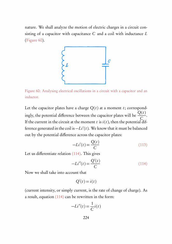
nature. We shall analyze the motion of electric charges in a circuit con-sisting of a capacitor with capacitance C and a coil with inductance L

(Figure 60).

Figure 60: Analysing electrical oscillations in a circuit with a capacitor and aninductor.

Let the capacitor plates have a charge Q(t ) at a moment t ; correspond-

ingly, the potential difference between the capacitor plates will beQ(t )

C.

If the current in the circuit at the moment t is i(t ), then the potential dif-ference generated in the coil is−Li ′(t ). We know that it must be balancedout by the potential difference across the capacitor plates:

−Li ′(t ) =Q(t )

C(113)

Let us differentiate relation (114). This gives

−Li ′′(t ) =Q ′(t )

C(114)

Now we shall take into account that

Q ′(t ) = i(t )

(current intensity, or simply current, is the rate of change of charge). Asa result, equation (114) can be rewritten in the form:

−Li ′′(t ) = 1C

i(t )

224

or

i ′′(t )+ 1LC

i(t ) = 0 (115)

The resultant differential equation is quite familiar, isn’t it?

Reader: This is a differential equation of type (80a) of the preceding

dialogue provided that q =1

LC. We con- clude, therefore, that the process

in the circuit is harmonic.

Author: Note, however, that the process is not that of mechanical vi-brations of a ball attached to springs but the process of electromagneticoscillations in an electric circuit.

Reader: As q =1

LCand using relation (94) of the previous dialogue,

we obtain a relation for the period of electromagnetic oscillations in thecircuit:

T = 2πp

LC (116)

The general solution of equation (115) is then

i(t ) =Asin�

1pLC

t +α�

(117)

Author: Absolutely correct. The two physical processes, namely, themechanical vibrations of a ball attached to springs and the electromagneticoscillations in a circuit, are mathematically similar. They are describedby the same differential equation. Otherwise you couldn’t write, nearlyautomatically as you did, the period of oscillations (formula (116) andthe general solution (formula 117).

In our dialogues we have discussed only two (and rather simple) typesof differential equations: those of exponential growth (decay) and of har-monic oscillations. And we have illustrated them with a number of phys-ical processes of very different kind.

225

Reader: I guess that the list of different differential equations, and cer-tainly the list of physical processes described by these equations, could besubstantially enlarged.

Author: No doubt. This concludes our discussion of differential equa-tions. I want to note in conclusion that differential equations are widelyapplied not only in physics but in chemistry, biology, cybernetics, soci-ology, and other fields of science as well.

226

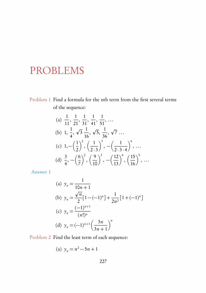
PROBLEMS

Problem 1 Find a formula for the nth term from the first several termsof the sequence:

(a)111

,121

,131

,141

,151

, . . .

(b) 1,14

,p

3116

,p

5,136

,p

7 . . .

(c) 1,−�

12

�2,�

12 · 3�3

, −�

12 · 3 · 4�4

, . . .

(d)34

, −�

67

�2,�

910

�3, −�

1213

�4,�

1516

�5, . . .

Answer 1

(a) yn =1

10n+ 1

(b) yn =p

n2[1− (−1)n]+

12n2[1+(−1)n]

(c) yn =(−1)n+1

(n!)n

(d) yn = (−1)n+1�

3n3n+ 1

�nProblem 2 Find the least term of each sequence:

(a) yn = n2− 5n+ 1

227

(b) yn = n+100n

(c) yn = n+ 5sinπn2

Answer 2

(a) y2 = y3 =−5

(b) y10 = 20

(c) y3 =−2

Problem 3 Find the largest term of each sequence:

(a) yn =90n

n2+ 9

(b) yn =10n

n!

Answer 3

(a) y3 = 15

(b) y9 = y10 =109

9!

Problem 4 Find which of the sequences given below are monotonic:

(a) yn = 3n2− n

(b) yn = n2− 3n

(c) yn = 7n− n2

(d) yn = log�

34

�nAnswer 4 (a) Increasing, (b) nondecreasing; (c) non-monotonic; (d) de-

creasing.

228

Problem 5 There are two sequences (yn ) and ( zn ) such that 0 ⩽ yn ⩽ zn

for all n. The sequence ( zn ) is convergent and its limit is zero.Prove that the sequence (yn ) is convergent to zero.

Problem 6 Prove that

(a) limn→∞

n2n= 0;

(b) limn→∞(p

n+ 1−pn− 1) = 0

Hint. In problem (a) transform

2n = (1+ 1)n =h1+ n+ + . . .i>�

n+n(n− 1)

2

�>

n2

2

and use the theorem proved in problem 5.

In problem (b) transform

pn+ 1−pn− 1=

2pn+ 1+

pn− 1

<2p

n− 1

and use the theorem proved above.

Problem 7 Find the limits of the following sequencers:

(a) yn =2n+

1n+ 3�p

n+p

3�2

(b) yn =5n2�

1+1n

�n1n− 3n2

(c) yn =

�1+

1n

�n+�

1+1

2n

�2n

2+1n+

1pn

229

(d) yn =2n + n

2n +p

n(p

n+ 1−pn− 1)

Answer 7 (a) 2; (b) −53

e ; (c) e ; (d) 0.

Problem 8 Find the function f (x) if 3 f (x − 1)− f�

1−xx

�= 2x.

Answer 8 f (x) =34(x + 1)+

14(x + 1)

.

Problem 9 Find analytical relations and the natural domains of the fol-lowing functions:

(a) f (1− x);

(b) f�

1x

�for f (x) = log(x2− 1),

Answer 9 (a) log(x2− 2x); x < 0, x > 2; (b) log1− x2

x2; 0< |x|< 1.

Problem 10 Analyze the continuity and differentiability of the functionf (x) = arcsin(s i nx) within the limits of the natural domainof the function.

Answer 10 The natural domain of the function f (x) is ]−∞,∞[; thefunction is continuous everywhere; it is differentiable at allpoints with the exception of points

x =±π2

, ±3π2

, ±5π2

, . . .

Problem 11 Prove that the function f (x) = 3p

x2 has no derivative at pointx = 0.

230

Problem 12 Prove that 3x6− 5x3− 30x < 40 if |x|⩽ 2.

Hint. Find first that the maximum value of the polynomialf (x) = 3x6 − 5x3 − 30x: over the interval [−2, 2] is below40. To do this, find the values of f (x) at the end points of theinterval [−2, 2] and at the points at which the derivative off (x) is zero (if these points belong to the indicated interval).

Problem 13 Find themaximum andminimumvalues of the function f (x) =x − 2 ln x over the interval [1, e].

Answer 13 The minimum value is f (2) = 2− 2 ln2, the maximum valueis f (1) = 1.

Problem 14 Find a point x0 at which the tangent to the graph of the func-tion f (x) = x2+ 1 is parallel to the straight line y = 3x.

Answer 14 x0 =32.

Problem 15 Write the equation of the tangent to the graph of the functionf (x) = x2− 4x + 5 at point x0 = 1.

Answer 15 y =−2x + 4.

Note. The equation of the tangent to the graph of the func-tion f (x) at x = x0 is: y = f (x0)+ f ′(x0)(x−x0), where f ′(x0)is the value of the derivative of the function at x0.

Problem 16 Find the derivatives of the following functions:

(a) f (x) = np

x;

(b) f (x) =1

x2+ 3;

(c) f (x) =p

x2+ 5;

231

(d) f (x) = tan2 x;

(e) f (x) = sin4 5x;

(f) f (x) = arcsinp

x;

(g) f (x) = lnx2− 1

10;

(h) f (x) = ln1+ xp1+ x2

.

Answer 16

(a)1

n np

xn−1;

(b) − 2x(x2+ 3)2

;

(c)xp

x2+ 5;

(d)2sin xcos2 x

;

(e) 20sin2 5x cos5x;

(f)1

2p

x(1− x);

(g)2x

x2− 1;

(h)1− x

(1+ x)(1+ x2).

Problem 17 Verify that the functions

F1 = cos2 x + cos4 x

F2 = cos2x − 14

sin2 2x

F3 = cos4 x + 3cos2 x + sin2 x

are the antiderivatives of one and the same function. FindF2− F1 and F3− F1.

232

Answer 17 F2− F1 = 1; F3− F1 = 2.

Problem 18 Find the area of the curvilinear trapezoid described by thegraph of the function f (x) = x2+1 over the inter- val [−3,3].

Answer 18 24.

Problem 19 Find the difference in areas of the curvilinear trapezoids de-fined by the graphs of the functions f1 = e x and f2 = e−x overthe interval [0,1].

Answer 19 e +1e.

Problem 20 Find the value of a minimizing the area of the curvilineartrapezoid defined by the graph of the function f (x) = (x −a)2+ a2 over the interval [0,1].

Answer 20 a =14.

Problem 21 Find the area of a figure bounded by the graph of the functionf (x) = x2− 2x + 2 and two tangents to this graph, drawn atpoints x1 = 0 and x2 = 2.

Answer 2123.

Problem 22 Find the numbers obtained by evaluating the integral∫ 2

1f (x)d x

of the following functions:

(a) f (x) =1x;

(b) f (x) =1x2;

(c) f (x) =1x3;

233

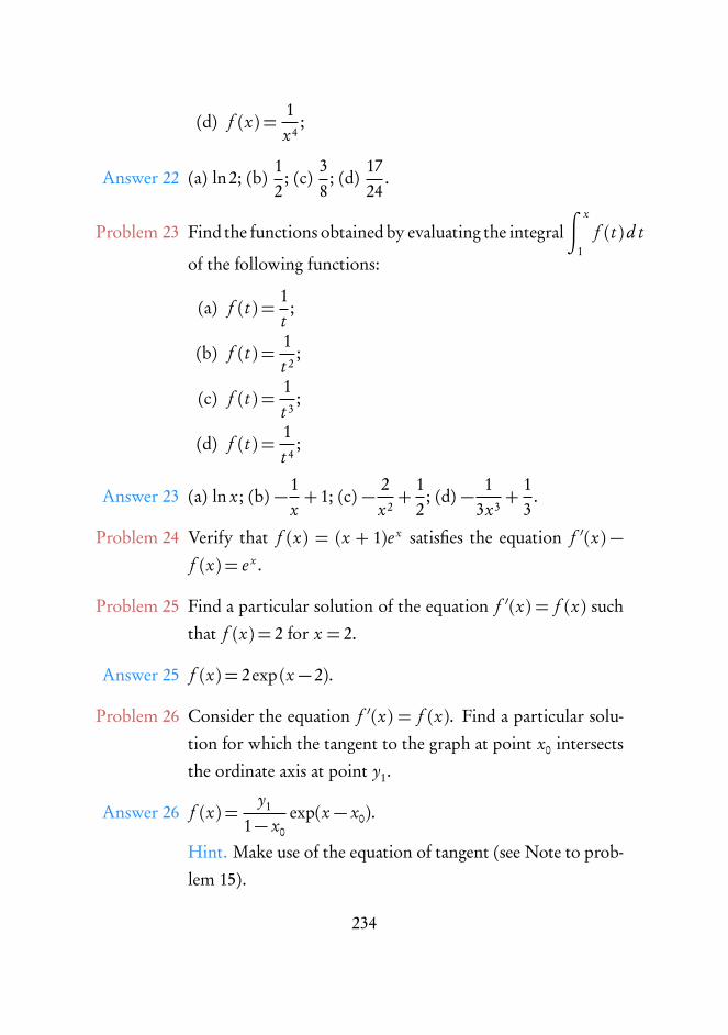
(d) f (x) =1x4;

Answer 22 (a) ln2; (b)12; (c)

38; (d)

1724

.

Problem 23 Find the functions obtained by evaluating the integral∫ x

1f (t )d t

of the following functions:

(a) f (t ) =1t;

(b) f (t ) =1t 2;

(c) f (t ) =1t 3;

(d) f (t ) =1t 4;

Answer 23 (a) ln x; (b) − 1x+ 1; (c) − 2

x2+

12; (d) − 1

3x3+

13.

Problem 24 Verify that f (x) = (x + 1)e x satisfies the equation f ′(x) −f (x) = e x .

Problem 25 Find a particular solution of the equation f ′(x) = f (x) suchthat f (x) = 2 for x = 2.

Answer 25 f (x) = 2exp (x − 2).

Problem 26 Consider the equation f ′(x) = f (x). Find a particular solu-tion for which the tangent to the graph at point x0 intersectsthe ordinate axis at point y1.

Answer 26 f (x) =y1

1− x0

exp(x − x0).

Hint. Make use of the equation of tangent (see Note to prob-lem 15).

234

Problem 27 Consider the graphs of different particular solutions of theequation f ′(x) = f (x). Verify that at the same point x0 thetangents to all these graphs intersect the abscissa axis at a com-mon point x = x0− 1.

Problem 28 Find the nth derivative of the following functions:

(a) f (x) = sin x;

(b) f (x) = cos x.

Answer 28

(a) f (x) = sin�

x +nπ2

�;

(b) f (x) = cos�

x +nπ2

�.

Problem 29 Find the value of the fourth derivative of the function f (x) =ln x for x = 2.

Answer 29 −38.

Problem 30 Find the area of the curvilinear trapezoid defined by the graphof the third derivative of the function f (x) = x5−2x2+ x−1

over the interval [0,1].

Answer 30 20.

235

236

MIR PUBLISHERS MOSCOW

e book introduces basic concepts of calculus for high school students. e book is presented as a relatively free-flowing dialogue between the AUTHOR and the READER. From one discussion to another the AUTHOR will lead the inquisitive and receptive READER to different notions, ideas, and theorems of calculus, emphasizing especially complicated or delicate aspects, stressing the inner logic of proofs, and attracting the reader's attention to special points. I hope that this form of presentation will help a reader of the book in learning new definitions such as those of derivative, antiderivative, definite. integral, differential equation, etc. e author also expects that it will lead the reader to better understanding of such concepts as numerical sequence, limit of sequence, and function.