L E IMAGE SUPER-RESOLUTION NETWORKS VIA STRUCTURE

Published as a conference paper at ICLR 2022

LEARNING EFFICIENT IMAGE SUPER-RESOLUTIONNETWORKS VIA STRUCTURE-REGULARIZED PRUNING

Yulun Zhang1,† Huan Wang1,†,∗ Can Qin1 Yun Fu1

1Northeastern University, USA

ABSTRACT

Several image super-resolution (SR) networks have been proposed for efficientSR, achieving promising results. However, they are still not lightweight enoughand neglect to be extended to larger networks. At the same time, model compres-sion methods (i.e., knowledge distillation and neural architecture search) usuallyneed heavy extra resources. Then, we turn to a cheap and effective model com-pression way: network pruning. However, it is not easy to directly apply networkpruning to image SR. It is well-known tricky to conduct filter pruning for resid-ual blocks commonly used in SR networks. To solve these problems, we proposestructure-regularized pruning (SRP), which imposes regularization on the prunedstructure to ensure the locations of pruned filters are aligned across different lay-ers. Specifically, for the layers connected by the same residual, we select thefilters of the same indices as unimportant filters. To transfer the expressive powerin the unimportant filters to the rest of the network, we employ L2 regularizationto drive the weights towards zero so that eventually, their absence will cause mini-mal performance degradation. We apply SRP to train efficient image SR networks,resulting in a lightweight network SRPN-Lite and a very deep one SRPN. We pro-vide extensive comparisons with both lightweight and larger image SR networks.Our SRPN-Lite and SRPN perform favorably against other recent works.

1 INTRODUCTION

Given a low-resolution (LR) image, single image super-resolution (SR) aims to reconstruct a high-resolution (HR) output. Essentially, as a many-to-one mapping problemimage SR is ill-posed. Totackle this problem, plenty of deep convolutional neural networks (CNNs) (Dong et al., 2014; 2016;Kim et al., 2016b; Zhang et al., 2018c; 2020; 2021) have been investigated to learn the accuratemapping from LR input to the corresponding HR target.

Deep CNN for image SR is first investigated in SRCNN (Dong et al., 2014) and has continuouslyshown promising SR performance. SRCNN consists of there convolutional (Conv) layers, constrain-ing its expressivity. Kim et al. adopted residual learning to increase network depth in VDSR (Kimet al., 2016a) and obtained notable improvements over SRCNN. Lim et al. (Lim et al., 2017) sim-plified residual blocks and built a much deeper network EDSR. Zhang et al. (Zhang et al., 2018b)proposed a even much deeper one RCAN with the residual in residual structure. Empowered byincreased network size, deep SR models like EDSR (Lim et al., 2017) and RCAN (Zhang et al.,2018b) have seen remarkable SR performance. However, as a cost, the large model size bringsabout problems such as excessive memory footprint, slow inference speed. It is thereby impracticalto deploy them on resource-constrained platforms directly (Lee et al., 2020).

Aiming for efficient SR, more and more works introduce lightweight network architectures (Ahnet al., 2018; Luo et al., 2020). Ahn et al. proposed cascading residual network (CARN) (Ahnet al., 2018). Hui et al. proposed information multi-distillation network (IMDN) (Hui et al., 2019).Lee et al. introduced knowledge distillation (Hinton et al., 2014) for image SR (Lee et al., 2020).Besides, neural architecture search (NAS) (Zoph & Le, 2017; Elsken et al., 2019) was also utilizedfor lightweight SR model (Chu et al., 2019a). However, there are still several downsides to thesenetworks: (1) There is still an obvious performance gap between those lightweight models and thevery deep models; (2) These methods can consume considerable computation resources for training.For example, (Chu et al., 2019a) train a single network with 8 Tesla V100 GPUs, and the training

†Equal contribution. The main work was done when Yulun Zhang was at Northeastern University.*Corresponding author: Huan Wang ([email protected])

1


HR (img 092) SRCNN LapSRN MemNet CARN IMDN SRPN-Lite (ours)

HR (img 063) EDSR SRFBN SAN CSNLN RFANet SRPN (ours)

Figure 1: Visual comparisons (×4) about lightweight and large SR networks on Urban100 dataset.The first row is lightweight SR networks comparison. The second row is about larger models com-parison. SRPN-Lite and SRPN are our proposed lightweight and larger image SR networks.

takes about three days; (3) It is hard for most lightweight SR network designs to generalize to morelarge-scale networks and achieve superior performance at the same time. So, it is needed to exploremore resource-friendly, effective, and generic lightweight SR networks.

On the other hand, neural network pruning is well-known as an effective technique to reduce modelcomplexity (Reed, 1993; Sze et al., 2017). For acceleration, filter pruning (a.k.a. structured prun-ing) (Li et al., 2017) attracts more attention than weight-element pruning (a.k.a. unstructured prun-ing) (Han et al., 2015; 2016b). Introducing filter pruning into image SR is a promising way toachieve a good trade-off between performance and complexity. However, it is not easy to apply fil-ter pruning techniques to image SR networks directly. This is mainly because residual connectionsare well-known difficult to prune in structured pruning (Li et al., 2017). On the other hand, they areextensively used in state-of-the-art (SOTA) image SR methods (e.g., EDSR (Lim et al., 2017) has 32residual blocks; RCAN (Zhang et al., 2018b) even has nested residual blocks).

To tackle the above issue, we propose Structure-Regularized Pruning (SRP), which imposes regu-larization on the pruned structure to ensure the locations of pruned filters are aligned across differentlayers. Specifically, for the layers connected by the same residual, we select the filters of the sameindices as unimportant filters (i.e., those we will remove finally). To transfer the expressive powerin the unimportant filters to the remainder of the network, we employ L2 regularization to drive theweights towards zero gradually so that eventually, their absence will incur negligible performanceloss. To the best of our knowledge, our SRP is one of the leading works (Zhang et al., 2021) toleverage structured pruning for efficient image SR. Our main contributions are as follows:

• We propose a network structure-regularized pruning (SRP) method to learn efficient imageSR networks. We try to jointly train image SR models with network pruning simultaneouslyto achieve high reconstruction performance as well as efficiency.

• Our SRP provides a general idea to structurally prune networks, which consists of extensiveresidual connections. The introduction of regularization as a pruning tool manages to main-tain the expressivity of the original network while peeling off the unnecessary redundancy.

• We employ SRP to train efficient image SR networks, resulting in a lightweight network(named SRPN-Lite) and a very deep one (named SRPN). We achieve superior performancegains on both lightweight and large image SR networks.

2 RELATED WORK

Deep Image SR Models. Dong et al. (Dong et al., 2014) firstly proposed SRCNN for image SRand achieved superior performance with only 3 convolutional (Conv) layers. Residual learning wasintroduced in VDSR (Kim et al., 2016a), reaching 20 Conv layers and a significant improvementover SRCNN. Tai et al. later introduced memory block in MemNet (Tai et al., 2017b) for deepernetwork structure. Lim et al. (Lim et al., 2017) simplified the residual block (He et al., 2016) andconstructed deeper and wider networks with a large number of parameters. Zhang et al. (Zhanget al., 2018b) proposed an even deeper one, residual channel attention network (RCAN), where theattention mechanism was firstly introduced in image SR. Liu et al. proposed FRANet (Liu et al.,2020) to make the residual features focus on critical spatial contents. Later, Zhang et al. (Zhanget al., 2019) extended to image restoration with residual non-local attention. Mei et al. proposedCSNLN (Mei et al., 2020) by combining local and non-local feature correlations. Most of thosemethods have achieved SOTA results. However, they suffer from huge model size (i.e., networkparameter number) and/or heavy computation operations (i.e., FLOPs).

2


(c)

𝒋 − 𝟏

𝒋 + 𝟏

𝒋

Fi-1 Fi Fi+1 Fi+2

Wi Wi+1

1

1

3

6

3

6

2

57

2

5

7

2

5

7

Short CutChannel Pruning

(b)(a)

Filter Pruning

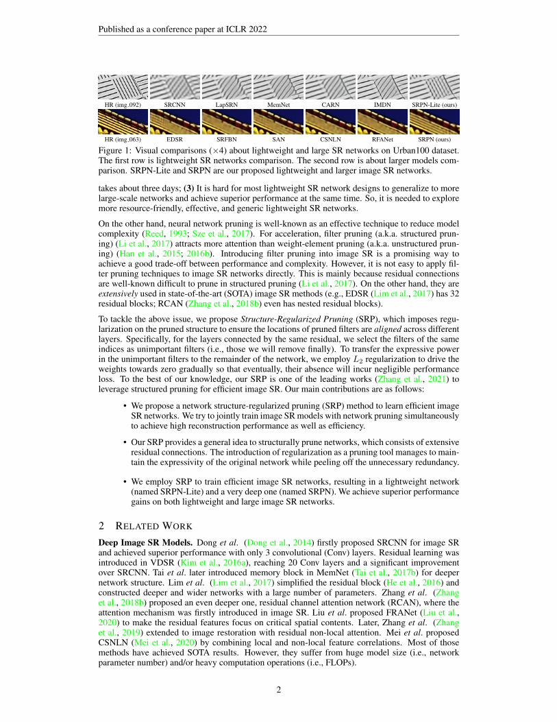
Figure 2: (a) Illustration of channel-wise and filter-wise pruning for single Conv layer. In this work,we adopt filter-wise pruning to learn efficient image SR networks. (b) Illustration of filter pruningwithin a residual block. We depict deep features F as 3d cubes. We expend the Conv kernel W (4dtensor) as a 2d matrix here for easy illustration (each row represents a filter). Both green and bluecolor denote the pruned filters (or feature map channels): green denotes the pruned filters in freeConv layers; blue denotes the pruned filters in constrained Conv layers. The basic idea of our SRPis to apply the L2 regularization to the unimportant filters to make sure the pruned indices of F (i)

are exactly the same as those of F (i+2). (c) Illustration of filter pruning across different residualblocks. All the layers that are directly followed by the add operators are constrained Conv layers (inblue). Others are free Conv layers (in green).

Lightweight Image SR Models. Recent years have been rising interest in investigating lightweightimage SR models. These approaches try to design lightweight architectures, which mainly takeadvantage of recursive learning and channel splitting. Kim et al. firstly decreased parameter num-ber by utilizing recursive learning in DRCN (Kim et al., 2016b). Ahn et al. proposed CARN bydesigning a cascading mechanism upon a residual network (Ahn et al., 2018). Hui et al. proposedIMDN by using distillation and fusion modules (Hui et al., 2019). Luo et al. designed the latticeblock with butterfly structures (Luo et al., 2020). Recently, neural architecture search was appliedfor image SR, like FALSR (Chu et al., 2019a). Also, model compression techniques have been ex-plored for image SR. He et al. proposed knowledge distillation based feature-affinity for efficientimage SR (He et al., 2020). Lee et al. distilled knowledge from a larger teacher network to a studentone (Lee et al., 2020). Those lightweight image SR models have obtained great progress, but westill need to investigate deeper for more efficient image SR models.

Neural Network Pruning. Network pruning aims to eliminate redundant parameters in a neu-ral network without compromising its performance seriously (Reed, 1993; Sze et al., 2017). Themethodology of pruning mainly falls into two groups: filter pruning (or more generally known asstructured pruning)* and weight-element pruning (also referred to as unstructured pruning). Theformer aims to remove weights by filters (i.e., 4-d tensors), while the latter removes weights by sin-gle elements (i.e., scalars). Structured pruning results in regular sparsity after pruning. It does notdemand any special hardware features to achieve considerable practical acceleration. In contrast,unstructured pruning leads to irregular sparsity. Leveraging the irregular sparsity for accelerationtypically demands special software supports, while past works have shown the practical speedup isvery limited (Wen et al., 2016), unless using customized hardware platforms (Han et al., 2016a).In this paper, we tackle filter pruning instead of weight-element pruning for effortless acceleration.The major efforts in pruning (mainly in image classification) have been focusing on proposing amore sound pruning criterion to select unimportant weights (Reed, 1993; Sze et al., 2017). Criteriabased on weight magnitude (Han et al., 2015; 2016b; Li et al., 2017) are the most prevailing ones,which we will also employ to develop our method in this paper.

3 METHODOLOGY

We first show the overview of the problem setting about deep CNN for image SR. It is also observedthat excessive redundancy exists in the SR deep CNNs. Then we move on to proposing our structure-regularized pruning (SRP) method attempting to achieve more efficient SR networks.

3.1 DEEP CNN FOR IMAGE SRIn image super-resolution (SR), a high-resolution (a.k.a. super-resolved) image ISR is reconstructedfrom its low-resolution (LR) input ILR. This image SR process can be described as

ISR = FSR(ILR; Θ), (1)

*Filter pruning is a sub-concept within structured pruning, while they are often used interchangeably in theliterature. In this paper, we stick to this terminology practice.

3


where FSR(·) is the image SR network, parameterized by Θ. Meanwhile, the LR input ILR fromthe corresponding HR image can be formulated as

ILR = F↓s(IHR), (2)where F↓s(·) downscales the original HR image IHR by a scale factor s. This downscaling pro-cess typically introduces additional compression, blurring, noise, and/or other unknown artifacts.Therein, the desired structural details could be removed more or less. The job of image SR methodsis to reconstruct the high-frequency information as much as possible.

We aim to present a structural sparsity inducing SR network learning method, which can delivermore efficient SR networks with fewer parameters and FLOPs.

3.2 STRUCTURE-REGULARIZED PRUNING (SRP)Pruned Index Constraint. Pruning filters in residual networks is well-known non-trivial as the Addoperators in residual blocks require the pruned filter indices across different residual blocks must bealigned. A figurative illustration of filter pruning within a residual block is shown in Fig. 2(b). Atypical residual block (e.g., in EDSR (Lim et al., 2017), RCAN (Zhang et al., 2018b)) consists oftwo convolutional layers. According to the mutual connection relationship, the convolutional layerscan be categorized into two groups. One group is made up with the layers that can be pruned withoutany constraint, dubbed free Conv layers in this work; the other comprises Conv layers whose filtersmust be pruned at the same indices, dubbed constrained Conv layers. Concretely, the layer W (i) inFig. 2(b) is a free Conv layer, while the layer W (i+1) is a constrained one.

Owing to the pruned index constraint problem, many filter pruning methods in image classificationsimply do not prune the last Conv layer in residual blocks (Li et al., 2017; Wang et al., 2021), whichcan still deliver considerable speedup of practical interest. Nevertheless, this doing-nothing solutioncan barely translate to the image SR networks if we target a considerable speedup. The root cause isthat image SR networks usually utilize many more residual blocks, and each block usually has onlytwo Conv layers. In some top-performing SR networks (e.g., RCAN Zhang et al. (2018b)), there areeven nested residual blocks. Taking EDSR for a concrete example, it has 32 residual blocks withtwo Conv layers within each block. If the 2nd Conv layer in a residual block is spared from pruning,half of the Conv layers will not be pruned. In other words, at best, we can only obtain 2× theoreticalacceleration measured by FLOPs reduction.

Given this issue, it is imperative to prune all the Conv layers in residual blocks, thus calling for anapproach to align the pruned indices of all constrained Conv layers. We then use regularization as apromising solution considering that it has been widely used before to impose priors on the sparsitystructure in classification (Reed, 1993; Wen et al., 2016; Wang et al., 2021).

Our SRP method is based on regularization to form desired hardware-friendly sparsity structure.Primarily, there are three questions to answer in SRP: (1) which pruning criterion is used to chooseunimportant filters; (2) which kind of regularization is chosen to induce sparsity; (3) how to schedulethe pruning process to make the algorithm robust and easy to use.

(1) Pruning Criterion. When it comes to formulated pruning criteria, they mainly fall into threegroups: magnitude based (Han et al., 2015; Li et al., 2017), 1st-order gradient based (Molchanovet al., 2017; 2019), and 2nd-order gradient based (LeCun et al., 1990; Hassibi & Stork, 1993; Wanget al., 2019a). The 1st-order and 2nd-order gradient-based criteria are based on Taylor approximationof the increased loss when a weight is removed, pioneered by (LeCun et al., 1990). They are moreaccurate than magnitude-based one right after pruning. However, pruning is typically followed bya finetuning process (Reed, 1993) to regain performance. After finetuning, the advantage of the1st-order and 2nd-order gradient-based criteria usually becomes marginal. Meanwhile, they aretypically more costly than the magnitude-based criteria. Taking the cost and flexibility into account,we simply employ magnitude-based pruning criteria.

Specifically, given a pretrained SR network, for all the free Conv layers, we sort the filters in as-cending order by their L1-norms and select the filers with the least norms as unimportant filters, bya predefined pruning ratio r ∈ (0, 1). For the constrained Conv layers, the problem becomes a littlebit more complex. Given the pruned index constraint, ideally, we can only prune the filters in theintersection set (denoted by S(net)) for the whole network,

S(net) =⋂l∈C

S(l), (3)

4


where S(l) represents the set of unimportant filters selected by certain pruning criterion in the l-thConv layer; C denotes the set of constrained Conv layers. For top-performed image SR networks,|C| (| · | denotes cardinality of a set) is at the order of magnitude of hundreds (e.g., |C| = 200for RCAN). Meanwhile, given a pretrained model, its pruned filter indices by L1-norm are usuallyrandom across different layers. As a consequence, |S(net)| will be rather small (in practice, onRCAN, we even observe |S(net)| = 0 when we try to prune 32 filters out of 64). This issue bringsmuch trouble to user control when we want to prune a layer to a pre-defined number of filters. Toaddress this issue, we choose to randomly select a set of filters as unimportant and fixed duringthe whole pruning process. In practice, we find this simple scheme works pretty well. The reasonenabling us to do so is that regularization for pruning is a gradual process. It allows ample timefor the network to recover from the introduced penalty term (this will be empirically verified in ourexperiments, see Fig. 3). Apart from aligning cross-layer sparsity structure, this is the second reasonwe choose regularization for pruning in our algorithm.

(2) Regularization Form. Although L1 regularization is well-known to induce sparsity in machinelearning, it is hard to tune the coefficient to realize a desired trade-off between sparsity and perfor-mance. Instead, L2 regularization is thereby adopted in our method given its more tamable controlover the sparsification process – note the gradient of L2 regularization is proportion to the weightmagnitude while the gradient of L1 regularization is not. Specifically, given the loss function L of aneural network Θ, the total error function E with adaptive L2 regularization term is formulated as

E(Θ;D) = L(Θ;D) +1

2

∑l,j

α(l)j ||W

(l)j ||

22, (4)

where D stands for the training dataset; W (l)j refers to the j-th filter in l-th Conv layer; α(l)

j standsfor the L2 regularization co-efficient for that filter. If a filter j falls into the set of unimportant filtersS(l), α(l)

j > 0; otherwise, α(l)j = 0 since we do not restrict the learning of important filters.

(3) Regularization Schedule. As mentioned above, for the constrained Conv layers, we select theunimportant filters randomly. To mitigate the side effect of this sub-optimal choice, the networkshould be provided with abundant training iterations to adapt so that it can transfer its expressivepower to the remaining part of the network. To achieve this goal, we choose to gradually increasethe penalty strength, drawing inspirations from (Wang et al., 2019b; 2021),

α(l)j = α

(l)j + ∆, (5)

where ∆ (a pre-defined constant) is a small amount that the penalty strength is increased each time.This design allows us to raise the penalty strength to a large amount eventually (like 0.5 in ourexperiments; in contrast, note the normal L2 regularization co-efficient is at the scale of 10−4). Asa result, the unimportant weights are driven rather close to zero, and removing them will hardly hurtthe performance. Besides, α is updated every T iterations during training for stability.

To indicate when to terminate the pruning process, a ceiling limit τ is introduced for the regulariza-tion co-efficient α. The pruning is over when all the α’s for unimportant filters arise to τ .

3.3 LEARNING EFFICIENT IMAGE SR MODELS VIA SRPSRP can be applied to top-performing SR algorithms in a plug-and-play manner – simply replacethe loss function L in Eq. (4) with the loss objective function of an SR approach of interest. Theproposed L2 regularization can be implemented on any deep learning framework very easily.

Upon finishing pruning, we take away the unimportant filters (not zeroing out them only, but literallyremoving them from the model), which will give us a compact SR model. Finally, the compact modelwill be finetuned to regain performance following the common practice in pruning (Reed, 1993).

3.4 IMPLEMENTATION DETAILS

We explain how to apply SRP to both lightweight and deep image SR networks to demonstrate themethod can work with a wide range of SR networks under different computation budgets.

Lightweight Networks. First, we adapt the EDSR baseline (Lim et al., 2017) with 16 residualblocks and remove its final Conv layer to reduce model size. The reconstruction upscaling is realizedby the pixel-shuffle layer (Shi et al., 2016) following common practice. The channel number in therevised EDSR baseline is first set as 256 and then pruned to 45. For×2 scale, we reduce the numberof parameters from 19.5M to 609K and name the compressed model as SRPN-Lite.

5


Pruning ratio Params (K) FLOPs (G) Scratch L1-norm pruning (Li et al., 2017) SRP (ours)0.1 1,101.8 254.5 37.85 37.91 37.970.3 681.1 157.7 37.81 37.81 37.890.5 381.8 88.9 37.75 37.73 37.840.7 154.2 36.5 37.56 37.58 37.710.9 26.9 7.3 36.74 36.87 37.28

Table 1: PSNR (dB) values on the Set5 (×2) between SRP and other two baselines to achieveexactly the same compact network. “Scratch” stands for training the small network from scratch.“L1-norm” removes filters with the smallest L1-norms. The unpruned model is EDSR baseline(Params: 1,369.9K, FLOPs: 316.3G, PSNR: 37.99 dB). The best results are highlighted.

0 20 40 60 80 100

Iteration (k)

0.00

0.02

0.04

0.06

Mea

nL

1-n

orm

model.body.12.body.0

Pruned filters

Kept filters

0 20 40 60 80 100

Iteration (k)

0.00

0.02

0.04

0.06

Mea

nL

1-n

orm

model.body.12.body.2

Pruned filters

Kept filters

Figure 3: Plots of the mean L1-norm of filters vs. iterations for “model.body.12.body.0” (free Convlayer) and “model.body.12.body.2” (constrained Conv layer) in EDSR baseline. As expected, theunimportant filters (“Pruned filters”) are driven down (owing to strong regularization); interestingly,the important ones arise spontaneously.

Deep Networks. To apply SRP to the very deep network RCAN (Zhang et al., 2018b), a representa-tive top-performing deep SR network with over 400 Conv layers, we revise RCAN by removing allthe channel attention modules (Zhang et al., 2018b). The channel number in the revised RCAN ischosen as 96 and then pruned to 64. For ×2 scale, we reduce the number of parameters from 34.5Mto 15.3M and dub the compressed model as SRPN.

4 EXPERIMENTAL RESULTS

4.1 SETTINGS

Data and Evaluation. We use DIV2K dataset (Timofte et al., 2017) and Flickr2K Lim et al. (2017)as training data, following most recent works (Timofte et al., 2017; Lim et al., 2017; Zhang et al.,2018a; Haris et al., 2018). For testing, we use five standard benchmark datasets: Set5 (Bevilacquaet al., 2012), Set14 (Zeyde et al., 2010), B100 (Martin et al., 2001), Urban100 (Huang et al., 2015),and Manga109 (Matsui et al., 2017). The SR results are evaluated with PSNR and SSIM (Wanget al., 2004) on the Y channel in YCbCr space.

Training Settings. Following (Zhang et al., 2018b), data augmentation is used in training – trainingimages are randomly rotated by 90◦, 180◦, 270◦ and flipped horizontally. Image patches (patchsize 48×48) are cropped out to form each training batch. Adam optimizer (Kingma & Ba, 2014) isadopted for training with β1=0.9, β2=0.999, and ε=10−8. Initial learning rate is set to 10−4 and thendecayed by factor 0.5 every 2×105 iterations. We use PyTorch (Paszke et al., 2017) to implementour models with a Tesla V100 GPU†.

4.2 ABLATION STUDY

The EDSR baseline with 16 residual blocks (Lim et al., 2017)‡ is used as the backbone for ablationstudy given its broad use in the community.

Comparison with Baseline Pruning Methods. To start with, we show that our SRP is more effec-tive than the available baseline compact image SR network learning methods. Two baseline methods

†The code is available at https://github.com/mingsun-tse/SRP.‡https://github.com/sanghyun-son/EDSR-PyTorch

6

https://github.com/MingSun-Tse/SRP

https://github.com/sanghyun-son/EDSR-PyTorch


Method Scale Params Mult-Adds Set5 Set14 B100 Urban100PSNR SSIM PSNR SSIM PSNR SSIM PSNR SSIM

SRCNN ×2 57K 52.7G 36.66 0.9542 32.42 0.9063 31.36 0.8879 29.50 0.8946FSRCNN ×2 12K 6.0G 37.00 0.9558 32.63 0.9088 31.53 0.8920 29.88 0.9020VDSR ×2 665K 612.6G 37.53 0.9587 33.03 0.9124 31.90 0.8960 30.76 0.9140DRCN ×2 1,774K 17,974.3G 37.63 0.9588 33.04 0.9118 31.85 0.8942 30.75 0.9133LapSRN ×2 813K 29.9G 37.52 0.9590 33.08 0.9130 31.80 0.8950 30.41 0.9100DRRN ×2 297K 6,796.9G 37.74 0.9591 33.23 0.9136 32.05 0.8973 31.23 0.9188MemNet ×2 677K 2,662.4G 37.78 0.9597 33.28 0.9142 32.08 0.8978 31.31 0.9195CARN ×2 1,592K 222.8G 37.76 0.9590 33.52 0.9166 32.09 0.8978 31.92 0.9256IMDN ×2 694K 158.8G 38.00 0.9605 33.63 0.9177 32.19 0.8996 32.17 0.9283SRPN-Lite (ours) ×2 609K 139.9G 38.10 0.9608 33.70 0.9189 32.25 0.9005 32.26 0.9294SRCNN ×3 57K 52.7G 32.75 0.9090 29.28 0.8209 28.41 0.7863 26.24 0.7989FSRCNN ×3 12K 5.0G 33.16 0.9140 29.43 0.8242 28.53 0.7910 26.43 0.8080VDSR ×3 665K 612.6G 33.66 0.9213 29.77 0.8314 28.82 0.7976 27.14 0.8279DRCN ×3 1,774K 17,974.3G 33.82 0.9226 29.76 0.8311 28.80 0.7963 27.15 0.8276DRRN ×3 297K 6,796.9G 34.03 0.9244 29.96 0.8349 28.95 0.8004 27.53 0.8378MemNet ×3 677K 2,662.4G 34.09 0.9248 30.00 0.8350 28.96 0.8001 27.56 0.8376CARN ×3 1,592K 118.8G 34.29 0.9255 30.29 0.8407 29.06 0.8034 28.06 0.8493IMDN ×3 703K 71.5G 34.36 0.9270 30.32 0.8417 29.09 0.8046 28.17 0.8519SRPN-Lite (ours) ×3 615K 62.7G 34.47 0.9276 30.38 0.8425 29.16 0.8061 28.22 0.8534SRCNN ×4 57K 52.7G 30.48 0.8628 27.49 0.7503 26.90 0.7101 24.52 0.7221FSRCNN ×4 12K 4.6G 30.71 0.8657 27.59 0.7535 26.98 0.7150 24.62 0.7280VDSR ×4 665K 612.6G 31.35 0.8838 28.01 0.7674 27.29 0.7251 25.18 0.7524DRCN ×4 1,774K 17,974.3G 31.53 0.8854 28.02 0.7670 27.23 0.7233 25.14 0.7510LapSRN ×4 813K 149.4G 31.54 0.8850 28.19 0.7720 27.32 0.7280 25.21 0.7560DRRN ×4 297K 6,796.9G 31.68 0.8888 28.21 0.7720 27.38 0.7284 25.44 0.7638MemNet ×4 677K 2,662.4G 31.74 0.8893 28.26 0.7723 27.40 0.7281 25.50 0.7630CARN ×4 1,592K 90.9G 32.13 0.8937 28.60 0.7806 27.58 0.7349 26.07 0.7837IMDN ×4 715K 40.9G 32.21 0.8948 28.58 0.7811 27.56 0.7353 26.04 0.7838SRPN-Lite (ours) ×4 623K 35.8G 32.24 0.8958 28.69 0.7836 27.63 0.7373 26.16 0.7875

Table 2: Quantitative results of lightweight SR networks. Best results are highlighted.

Urban100: img 020 (×4)

HR Bicubic SRCNN FSRCNN VDSR

LapSRN MemNet CARN IMDN SRPN-Lite (ours)

Urban100: img 024 (×4)

HR Bicubic SRCNN FSRCNN VDSR

LapSRN MemNet CARN IMDN SRPN-Lite (ours)

Figure 4: Visual comparison of different lightweight SR approaches on the Urban100 dataset (×4).

are compared to: training from scratch and the original L1-norm pruning (Li et al., 2017). The re-sults are presented in Tab. 1. As we can see, our pruned network delivers the best PSNR consistentlyacross different pruning ratios. Notably, under a greater pruning ratio, the advantage of our methodover scratch training or L1-norm pruning is more evident in general, suggesting that our SRP is morevaluable in aggressive pruning cases. Of particular note is that, our method SRP also utilizes theL1-norm as the scoring criterion to select unimportant filters, same as (Li et al., 2017). Nevertheless,our method delivers significantly better results than theirs. The primary reason is that they do notimpose any regularization on the pruned structure; the remaining feature maps are thus mismatchedin residual blocks after pruning. In contrast, our method SRP is not bothered by this issue, showingthe effectiveness of our proposed structure regularization.

Visualization of Pruning Process. In Fig. 3, we visualize the pruning process by plotting the meanL1-norm of filters in two layers of EDSR baseline during SRP training. The filters are split into twogroups, kept filters and pruned filters. As is shown in the figure, the mean L1-norm of the prunedfilters goes down gradually because the penalty grows stronger and stronger, driving them towardszero. Interestingly, note the L1-norms of the kept filters arise themselves. Recall that there is noexplicit regularization to promote them to grow. In other words, the network learns to recover byitself, akin to the compensation effect found in human brain (Duffau et al., 2003).

7


Method Scale Set5 Set14 B100 Urban100 Manga109PSNR SSIM PSNR SSIM PSNR SSIM PSNR SSIM PSNR SSIM

EDSR ×2 38.11 0.9602 33.92 0.9195 32.32 0.9013 32.93 0.9351 39.10 0.9773DBPN ×2 38.09 0.9600 33.85 0.9190 32.27 0.9000 32.55 0.9324 38.89 0.9775RCAN ×2 38.27 0.9614 34.12 0.9216 32.41 0.9027 33.34 0.9384 39.44 0.9786SRFBN ×2 38.11 0.9609 33.82 0.9196 32.29 0.9010 32.62 0.9328 39.08 0.9779SAN ×2 38.31 0.9620 34.07 0.9213 32.42 0.9028 33.10 0.9370 39.32 0.9792HAN ×2 38.27 0.9614 34.16 0.9217 32.41 0.9027 33.35 0.9385 39.46 0.9785IGNN ×2 38.24 0.9613 34.07 0.9217 32.41 0.9025 33.23 0.9383 39.35 0.9786CSNLN ×2 38.28 0.9616 34.12 0.9223 32.40 0.9024 33.25 0.9386 39.37 0.9785RFANet ×2 38.26 0.9615 34.16 0.9220 32.41 0.9026 33.33 0.9389 39.44 0.9783SRPN (ours) ×2 38.34 0.9619 34.29 0.9232 32.47 0.9032 33.50 0.9401 39.76 0.9796EDSR ×3 34.65 0.9280 30.52 0.8462 29.25 0.8093 28.80 0.8653 34.17 0.9476RCAN ×3 34.74 0.9299 30.65 0.8482 29.32 0.8111 29.09 0.8702 34.44 0.9499SRFBN ×3 34.70 0.9292 30.51 0.8461 29.24 0.8084 28.73 0.8641 34.18 0.9481SAN ×3 34.75 0.9300 30.59 0.8476 29.33 0.8112 28.93 0.8671 34.30 0.9494HAN ×3 34.75 0.9299 30.67 0.8483 29.32 0.8110 29.10 0.8705 34.48 0.9500IGNN ×3 34.72 0.9298 30.66 0.8484 29.31 0.8105 29.03 0.8696 34.39 0.9496CSNLN ×3 34.74 0.9300 30.66 0.8482 29.33 0.8105 29.13 0.8712 34.45 0.9502RFANet ×3 34.79 0.9300 30.67 0.8487 29.34 0.8115 29.15 0.8720 34.59 0.9506SRPN (ours) ×3 34.84 0.9303 30.76 0.8497 29.39 0.8120 29.36 0.8749 34.88 0.9515EDSR ×4 32.46 0.8968 28.80 0.7876 27.71 0.7420 26.64 0.8033 31.02 0.9148SRMDNF ×4 31.96 0.8925 28.35 0.7787 27.49 0.7337 25.68 0.7731 30.09 0.9024RCAN ×4 32.63 0.9002 28.87 0.7889 27.77 0.7436 26.82 0.8087 31.22 0.9173SRFBN ×4 32.47 0.8983 28.81 0.7868 27.72 0.7409 26.60 0.8015 31.15 0.9160SAN ×4 32.64 0.9003 28.92 0.7888 27.78 0.7436 26.79 0.8068 31.18 0.9169HAN ×4 32.64 0.9002 28.90 0.7890 27.80 0.7442 26.85 0.8094 31.42 0.9177IGNN ×4 32.57 0.8998 28.85 0.7891 27.77 0.7434 26.84 0.8090 31.28 0.9182CSNLN ×4 32.68 0.9004 28.95 0.7888 27.80 0.7439 27.22 0.8168 31.43 0.9201RFANet ×4 32.66 0.9004 28.88 0.7894 27.79 0.7442 26.92 0.8112 31.41 0.9187SRPN (ours) ×4 32.72 0.9010 29.04 0.7917 27.87 0.7457 27.25 0.8172 31.82 0.9221

Table 3: Quantitative results of large SR networks. Best results are highlighted.

Urban100: img 044 (×4)

HR Bicubic EDSR DBPN RCAN

SRFBN IGNN CSNLN RFANet SRPN (ours)

Urban100: img 062 (×4)

HR Bicubic EDSR DBPN RCAN

SRFBN IGNN CSNLN RFANet SRPN (ours)

Figure 5: Visual comparison of different large SR networks on the Urban100 dataset (×4).

4.3 COMPARISONS WITH LIGHTWEIGHT NETWORKS

We compare our SRPN-Lite with lightweight SR networks: SRCNN (Dong et al., 2014), FSR-CNN (Dong et al., 2016), VDSR (Kim et al., 2016a), DRCN (Kim et al., 2016b), LapSRN (Laiet al., 2017), DRRN (Tai et al., 2017a), MemNet (Tai et al., 2017b), CARN (Ahn et al., 2018) andIMDN (Hui et al., 2019). The compared results are produced from their released code.

Performance Comparisons. Table 2 shows PSNR/SSIM comparisons for ×2, ×3, and ×4 SR.When compared with previous leading models, our SRPN-Lite obtains the best performance onall benchmarks and scaling factors. Unlike most comparison methods, which achieve efficiencythrough careful network designs, our work starts with the existing EDSR baseline (Lim et al., 2017)and prunes it to a much smaller network, showing the effectiveness of our proposed SRP.

Model Size and Mult-Adds. Our SRPN-Lite has the fewest parameter number in comparison torecent efficient SR works such as MemNet, CARN, and IMDN. The comparison in terms of Mult-Adds (measured when the output size is set to 3×1,280×720) is also presented. As seen, our SRPN-Lite costs fewer Mult-Adds than most comparison methods. These results demonstrate the merits ofSRP against other counterparts in striking a better network performance-complexity trade-off.

8


Method Params Mult-Adds Set5 Set14 B100 Urban100MoreMNAS-A (Chu et al., 2019b) 1,039K 238.6G 37.63 33.23 31.95 31.24FALSR-A (Chu et al., 2019a) 1,021K 234.7G 37.82 33.55 32.12 31.93CARN+KD (Lee et al., 2020) 1,592K 222.8G 37.82 N/A 32.08 N/ASRPN-Lite (ours) 609K 139.9G 38.10 33.70 32.25 32.26

Table 4: Model complexity comparisons (×2). Output size is 3×1,280×720 to calculate Mult-Adds.

Visual Comparisons. The visual comparisons at ×4 scale are shown in Fig. 4. It is easy to see thatmost of the comparison algorithms can barely recover the lost texture details in the correct direction;moreover, they suffer from blurring artifacts. In stark contrast, our SRPN-Lite effectively alleviatesthe blurring artifacts and recovers sharper structural fine textures in the right way, justifying theperformance superiority of our SRP approach over other methods.

4.4 COMPARISONS WITH LARGER NETWORKS

Most previous lightweight SR networks neglect to extend their models to deeper and compare withlarger networks. As stated in Sec. 3.4, we extend our SRP method to larger network training andobtain a deeper network SRPN. In Tab. 3, we compare with large SR networks: EDSR (Lim et al.,2017), DBPN (Haris et al., 2018), RCAN (Zhang et al., 2018b), SRFBN (Li et al., 2019), SAN (Daiet al., 2019), HAN (Niu et al., 2020), IGNN (Zhou et al., 2020), CSNLN (Mei et al., 2020), andRFANet (Liu et al., 2020). The compared results are produced from their released code.

Performance Comparisons. In Tab. 3, we observe that our SRPN achieves the best PSNR/SSIMvalues across different test sets and scales, except for SSIM value on Set5 (×2). Our SRPN utilizesslightly fewer parameters (15.3M vs. 15.4M) with the same network depth as RCAN (Zhang et al.,2018b). Notably, our SRPN removes the channel attention module in RCAN, but still achieves betterresults. This is mainly because our SRPN is initially trained from a wider and stronger network (with96 channels). We train the much larger network and then prune it to the target size.

Visual Comparisons. We further show visual comparisons with larger networks (e.g., CSNLN,RFANet, and IGNN) in Fig. 5, we can also observe similar situations as in Fig. 4. For example, inimg 011, other methods suffer from heavy blurring artifacts. In other cases, they may not recoverclear structures in img 044 or even wrong details in img 062. Our SRPN achieves more visuallypleasing results with more structural details. Those comparisons demonstrate that our SRP methodcan be applied to train larger networks and obtain comparable or even better performance.

4.5 MORE COMPARISON WITH MODEL COMPRESSION TECHNIQUES

We further compare our SRP to other representative efficient image SR approaches via model com-pression. Concretely, neural architecture search based methods (Chu et al., 2019b;a) and knowledgedistillation (KD) based methods (Lee et al., 2020) are compared to. Quantitative results at ×2 scaleare presented in Tab. 4, where our SRPN-Lite delivers better PSNR results across different datasetswith fewer parameters and Mult-Adds. With our SRP pruning method, there is no need to searchmassive network architectures or pretraining a teacher network, which usually consumes consider-able computation resources. These comparisons show that our SRP, as a network pruning method,has as much potential (if not more) as other model compression techniques for efficient image SR.

5 CONCLUSION

Existing efficient image SR methods have achieved promising results with moderate model param-eters and Mult-Adds. However, they neglect to extend their approaches to larger networks, whichusually perform much better with more parameters and/or operations with residual learning. Mean-while, although model compression approaches, like knowledge distillation and neural architecturesearch, have also been exploited for efficient image SR networks, they typically demand excessivecomputation resources. As another promising model compression method, network pruning is hardto be incorporated into lightweight SR models directly. To address these issues, we present structure-regularized pruning (SRP), which imposes L2 regularization on the pruned structure to align thelocations of pruned filters across different layers. It can transfer the expressive power in the unim-portant filters to the remaining part of the network. We employ SRP to train both lightweight andlarge image SR networks, resulting in a lightweight network SRPN-Lite and a very deep one SRPN,delivering superior performance over recent SOTA efficient SR methods.Acknowledgments. This research is supported by the U.S. Army Research Office Award W911NF-17-1-0367.

9


REFERENCES

Namhyuk Ahn, Byungkon Kang, and Kyung-Ah Sohn. Fast, accurate, and lightweight super-resolution withcascading residual network. In ECCV, 2018. 1, 3, 8

Marco Bevilacqua, Aline Roumy, Christine Guillemot, and Marie Line Alberi-Morel. Low-complexity single-image super-resolution based on nonnegative neighbor embedding. In BMVC, 2012. 6

Xiangxiang Chu, Bo Zhang, Hailong Ma, Ruijun Xu, and Qingyuan Li. Fast, accurate and lightweight super-resolution with neural architecture search. arXiv preprint arXiv:1901.07261, 2019a. 1, 3, 9

Xiangxiang Chu, Bo Zhang, Ruijun Xu, and Hailong Ma. Multi-objective reinforced evolution in mobile neuralarchitecture search. arXiv preprint arXiv:1901.01074, 2019b. 9

Tao Dai, Jianrui Cai, Yongbing Zhang, Shu-Tao Xia, and Lei Zhang. Second-order attention network for singleimage super-resolution. In CVPR, 2019. 9

Chao Dong, Chen Change Loy, Kaiming He, and Xiaoou Tang. Learning a deep convolutional network forimage super-resolution. In ECCV, 2014. 1, 2, 8

Chao Dong, Chen Change Loy, and Xiaoou Tang. Accelerating the super-resolution convolutional neuralnetwork. In ECCV, 2016. 1, 8

H Duffau, L Capelle, D Denvil, N Sichez, P Gatignol, M Lopes, MC Mitchell, JP Sichez, and R Van Effenterre.Functional recovery after surgical resection of low grade gliomas in eloquent brain: hypothesis of braincompensation. Journal of Neurology, Neurosurgery & Psychiatry, 74(7):901–907, 2003. 7

Thomas Elsken, Jan Hendrik Metzen, and Frank Hutter. Neural architecture search: A survey. JMLR, 2019. 1

S. Han, X. Liu, and H. Mao. EIE: efficient inference engine on compressed deep neural network. ACM SigarchComputer Architecture News, 44(3):243–254, 2016a. 3

Song Han, Jeff Pool, John Tran, and William J Dally. Learning both weights and connections for efficientneural network. In NeurIPS, 2015. 2, 3, 4

Song Han, Huizi Mao, and William J Dally. Deep compression: Compressing deep neural networks withpruning, trained quantization and huffman coding. In ICLR, 2016b. 2, 3

Muhammad Haris, Greg Shakhnarovich, and Norimichi Ukita. Deep back-projection networks for super-resolution. In CVPR, 2018. 6, 9

B. Hassibi and D. G. Stork. Second order derivatives for network pruning: Optimal brain surgeon. In NeurIPS,1993. 4

Kaiming He, Xiangyu Zhang, Shaoqing Ren, and Jian Sun. Deep residual learning for image recognition. InCVPR, 2016. 2

Zibin He, Tao Dai, Jian Lu, Yong Jiang, and Shu-Tao Xia. Fakd: Feature-affinity based knowledge distillationfor efficient image super-resolution. In ICIP, 2020. 3

Geoffrey Hinton, Oriol Vinyals, and Jeff Dean. Distilling the knowledge in a neural network. In NeurIPSWorkshop, 2014. 1

Jia-Bin Huang, Abhishek Singh, and Narendra Ahuja. Single image super-resolution from transformed self-exemplars. In CVPR, 2015. 6

Zheng Hui, Xinbo Gao, Yunchu Yang, and Xiumei Wang. Lightweight image super-resolution with informationmulti-distillation network. In ACM MM, 2019. 1, 3, 8

Jiwon Kim, Jung Kwon Lee, and Kyoung Mu Lee. Accurate image super-resolution using very deep convolu-tional networks. In CVPR, 2016a. 1, 2, 8

Jiwon Kim, Jung Kwon Lee, and Kyoung Mu Lee. Deeply-recursive convolutional network for image super-resolution. In CVPR, 2016b. 1, 3, 8

Diederik Kingma and Jimmy Ba. Adam: A method for stochastic optimization. In ICLR, 2014. 6

Wei-Sheng Lai, Jia-Bin Huang, Narendra Ahuja, and Ming-Hsuan Yang. Deep laplacian pyramid networks forfast and accurate super-resolution. In CVPR, 2017. 8

10


Y. LeCun, J. S. Denker, and S. A. Solla. Optimal brain damage. In NeurIPS, 1990. 4

Wonkyung Lee, Junghyup Lee, Dohyung Kim, and Bumsub Ham. Learning with privileged information forefficient image super-resolution. In ECCV, 2020. 1, 3, 9

Hao Li, Asim Kadav, Igor Durdanovic, Hanan Samet, and Hans Peter Graf. Pruning filters for efficient convnets.In ICLR, 2017. 2, 3, 4, 6, 7

Zhen Li, Jinglei Yang, Zheng Liu, Xiaomin Yang, Gwanggil Jeon, and Wei Wu. Feedback network for imagesuper-resolution. In CVPR, 2019. 9

Bee Lim, Sanghyun Son, Heewon Kim, Seungjun Nah, and Kyoung Mu Lee. Enhanced deep residual networksfor single image super-resolution. In CVPRW, 2017. 1, 2, 4, 5, 6, 8, 9

Jie Liu, Wenjie Zhang, Yuting Tang, Jie Tang, and Gangshan Wu. Residual feature aggregation network forimage super-resolution. In CVPR, 2020. 2, 9

Xiaotong Luo, Yuan Xie, Yulun Zhang, Yanyun Qu, Cuihua Li, and Yun Fu. Latticenet: Towards lightweightimage super-resolution with lattice block. In ECCV, 2020. 1, 3

David Martin, Charless Fowlkes, Doron Tal, and Jitendra Malik. A database of human segmented naturalimages and its application to evaluating segmentation algorithms and measuring ecological statistics. InICCV, 2001. 6

Yusuke Matsui, Kota Ito, Yuji Aramaki, Azuma Fujimoto, Toru Ogawa, Toshihiko Yamasaki, and KiyoharuAizawa. Sketch-based manga retrieval using manga109 dataset. Multimedia Tools and Applications, 2017.6

Yiqun Mei, Yuchen Fan, Yuqian Zhou, Lichao Huang, Thomas S Huang, and Humphrey Shi. Image super-resolution with cross-scale non-local attention and exhaustive self-exemplars mining. In CVPR, 2020. 2,9

P. Molchanov, S. Tyree, and T. Karras. Pruning convolutional neural networks for resource efficient inference.In ICLR, 2017. 4

Pavlo Molchanov, Arun Mallya, Stephen Tyree, Iuri Frosio, and Jan Kautz. Importance estimation for neuralnetwork pruning. In CVPR, 2019. 4

Ben Niu, Weilei Wen, Wenqi Ren, Xiangde Zhang, Lianping Yang, Shuzhen Wang, Kaihao Zhang, XiaochunCao, and Haifeng Shen. Single image super-resolution via a holistic attention network. In ECCV, 2020. 9

Adam Paszke, Sam Gross, Soumith Chintala, Gregory Chanan, Edward Yang, Zachary DeVito, Zeming Lin,Alban Desmaison, Luca Antiga, and Adam Lerer. Automatic differentiation in pytorch. 2017. 6

R. Reed. Pruning algorithms – a survey. IEEE Transactions on Neural Networks, 4(5):740–747, 1993. 2, 3, 4,5

Wenzhe Shi, Jose Caballero, Ferenc Huszar, Johannes Totz, Andrew P Aitken, Rob Bishop, Daniel Rueckert,and Zehan Wang. Real-time single image and video super-resolution using an efficient sub-pixel convolu-tional neural network. In CVPR, 2016. 5

Vivienne Sze, Yu-Hsin Chen, Tien-Ju Yang, and Joel S Emer. Efficient processing of deep neural networks: Atutorial and survey. Proceedings of the IEEE, 105(12):2295–2329, 2017. 2, 3

Ying Tai, Jian Yang, and Xiaoming Liu. Image super-resolution via deep recursive residual network. In CVPR,2017a. 8

Ying Tai, Jian Yang, Xiaoming Liu, and Chunyan Xu. Memnet: A persistent memory network for imagerestoration. In ICCV, 2017b. 2, 8

Radu Timofte, Eirikur Agustsson, Luc Van Gool, Ming-Hsuan Yang, Lei Zhang, Bee Lim, Sanghyun Son,Heewon Kim, Seungjun Nah, Kyoung Mu Lee, et al. Ntire 2017 challenge on single image super-resolution:Methods and results. In CVPRW, 2017. 6

Chaoqi Wang, Roger Grosse, Sanja Fidler, and Guodong Zhang. Eigendamage: Structured pruning in thekronecker-factored eigenbasis. In ICML, 2019a. 4

Huan Wang, Xinyi Hu, Qiming Zhang, Yuehai Wang, Lu Yu, and Haoji Hu. Structured pruning for efficientconvolutional neural networks via incremental regularization. IEEE Journal of Selected Topics in SignalProcessing, 14(4):775–788, 2019b. 5

11


Huan Wang, Can Qin, Yulun Zhang, and Yun Fu. Neural pruning via growing regularization. In ICLR, 2021.4, 5

Zhou Wang, Alan C Bovik, Hamid R Sheikh, and Eero P Simoncelli. Image quality assessment: from errorvisibility to structural similarity. TIP, 2004. 6

Wei Wen, Chunpeng Wu, Yandan Wang, Yiran Chen, and Hai Li. Learning structured sparsity in deep neuralnetworks. In NeurIPS, 2016. 3, 4

Roman Zeyde, Michael Elad, and Matan Protter. On single image scale-up using sparse-representations. InProc. 7th Int. Conf. Curves Surf., 2010. 6

Kai Zhang, Wangmeng Zuo, and Lei Zhang. Learning a single convolutional super-resolution network formultiple degradations. In CVPR, 2018a. 6

Yulun Zhang, Kunpeng Li, Kai Li, Lichen Wang, Bineng Zhong, and Yun Fu. Image super-resolution usingvery deep residual channel attention networks. In ECCV, 2018b. 1, 2, 4, 6, 9

Yulun Zhang, Yapeng Tian, Yu Kong, Bineng Zhong, and Yun Fu. Residual dense network for image super-resolution. In CVPR, 2018c. 1

Yulun Zhang, Kunpeng Li, Kai Li, Bineng Zhong, and Yun Fu. Residual non-local attention networks for imagerestoration. In ICLR, 2019. 2

Yulun Zhang, Yapeng Tian, Yu Kong, Bineng Zhong, and Yun Fu. Residual dense network for image restora-tion. TPAMI, 2020. 1

Yulun Zhang, Huan Wang, Can Qin, and Yun Fu. Aligned structured sparsity learning for efficient imagesuper-resolution. NeurIPS, 2021. 1, 2

Shangchen Zhou, Jiawei Zhang, Wangmeng Zuo, and Chen Change Loy. Cross-scale internal graph neuralnetwork for image super-resolution. In NeurIPS, 2020. 9

Barret Zoph and Quoc Le. Neural architecture search with reinforcement learning. In ICLR, 2017. 1

12

Documents

L E IMAGE SUPER-RESOLUTION NETWORKS VIA STRUCTURE