Embed Size (px)
Citation preview
L Berkley DavisCopyright 2009
MER035: Engineering ReliabilityLecture 6
1
MER301: Engineering Reliability
LECTURE 6:
Chapter 3: 3.9, 3.11 and ReliabilityExponential Distributions, Independence and Joint Distributions, Reliability
L Berkley DavisCopyright 2009
MER301: Engineering ReliabilityLecture 6
2
Summary
Exponential Distribution
Independence
Joint Distributions
Reliability
L Berkley DavisCopyright 2009
MER301: Engineering ReliabilityLecture 6
3
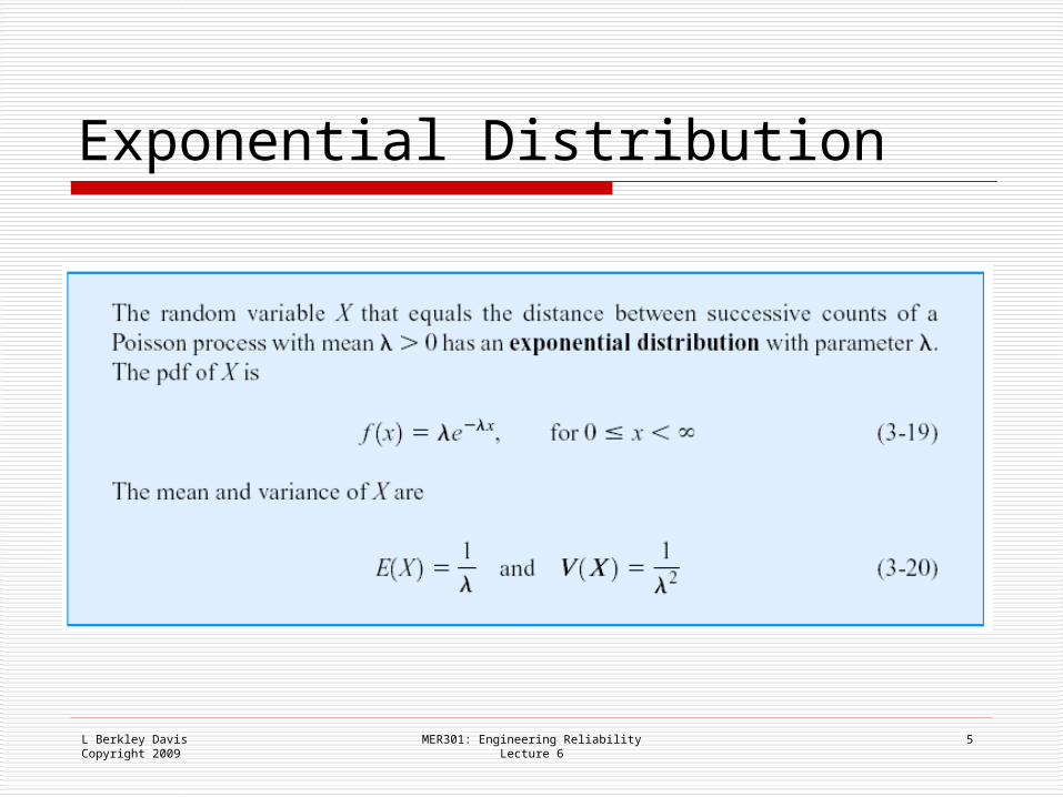
Exponential Distribution
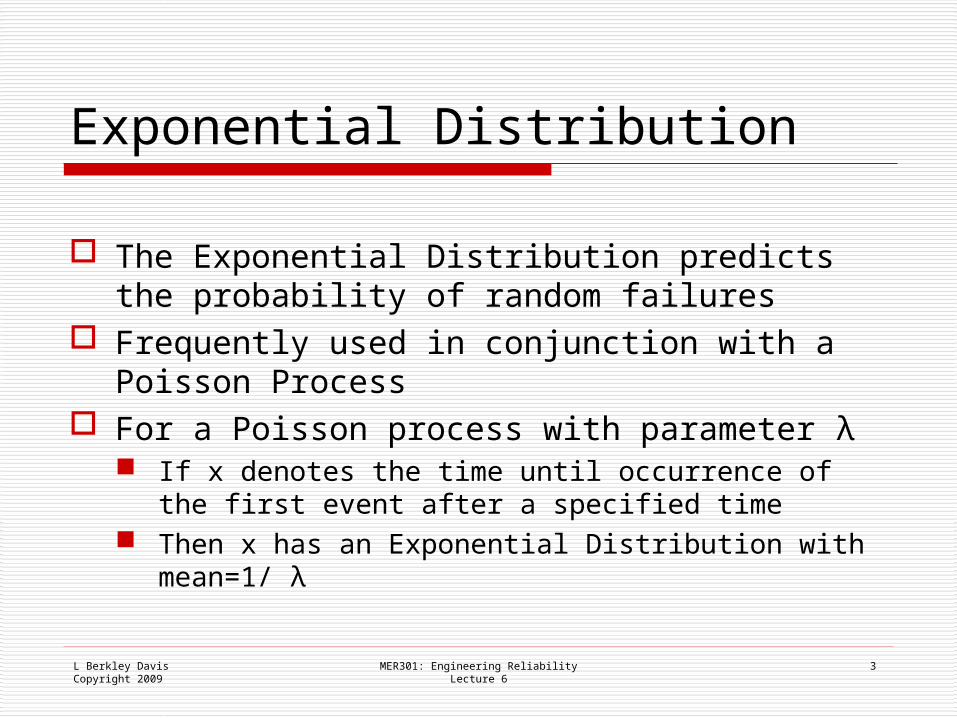
The Exponential Distribution predicts the probability of random failures
Frequently used in conjunction with a Poisson Process
For a Poisson process with parameter λ If x denotes the time until occurrence of the first
event after a specified time Then x has an Exponential Distribution with
mean=1/ λ
L Berkley DavisCopyright 2009
MER301: Engineering ReliabilityLecture 5
4
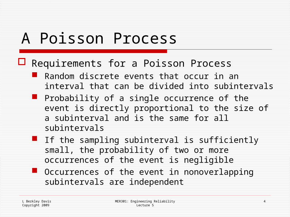
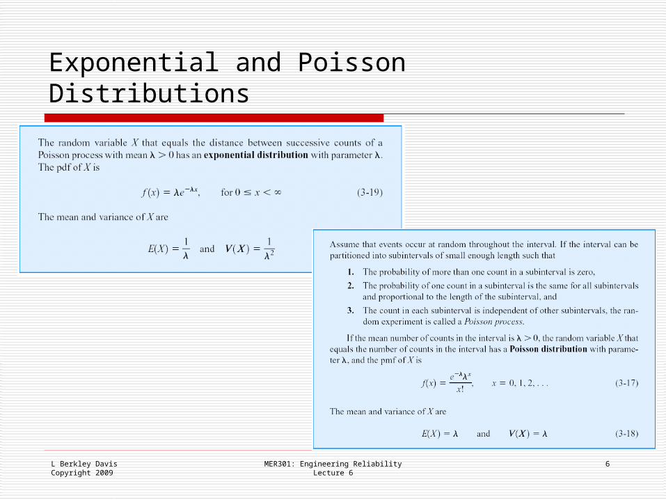
A Poisson Process Requirements for a Poisson Process
Random discrete events that occur in an interval that can be divided into subintervals
Probability of a single occurrence of the event is directly proportional to the size of a subinterval and is the same for all subintervals
If the sampling subinterval is sufficiently small, the probability of two or more occurrences of the event is negligible
Occurrences of the event in nonoverlapping subintervals are independent
L Berkley DavisCopyright 2009
MER301: Engineering ReliabilityLecture 6
5
Exponential Distribution
L Berkley DavisCopyright 2009
Exponential and Poisson Distributions
MER301: Engineering ReliabilityLecture 6
6
L Berkley DavisCopyright 2009
MER301: Engineering ReliabilityLecture 6
7
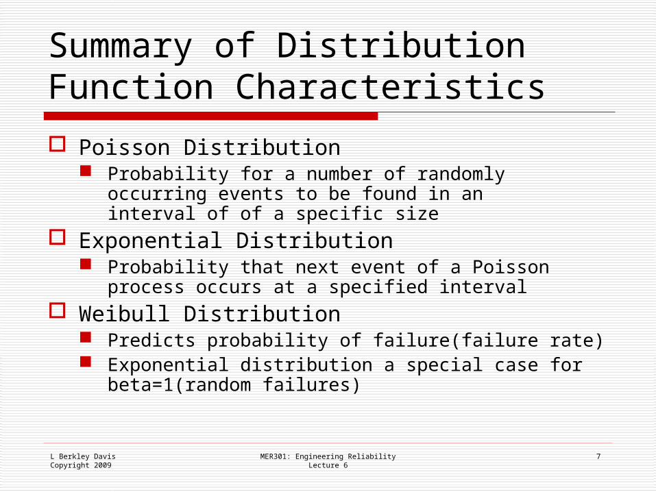
Summary of Distribution Function Characteristics Poisson Distribution
Probability for a number of randomly occurring events to be found in an interval of of a specific size
Exponential Distribution Probability that next event of a Poisson process
occurs at a specified interval Weibull Distribution
Predicts probability of failure(failure rate) Exponential distribution a special case for
beta=1(random failures)
L Berkley DavisCopyright 2009
MER301: Engineering ReliabilityLecture 6
8
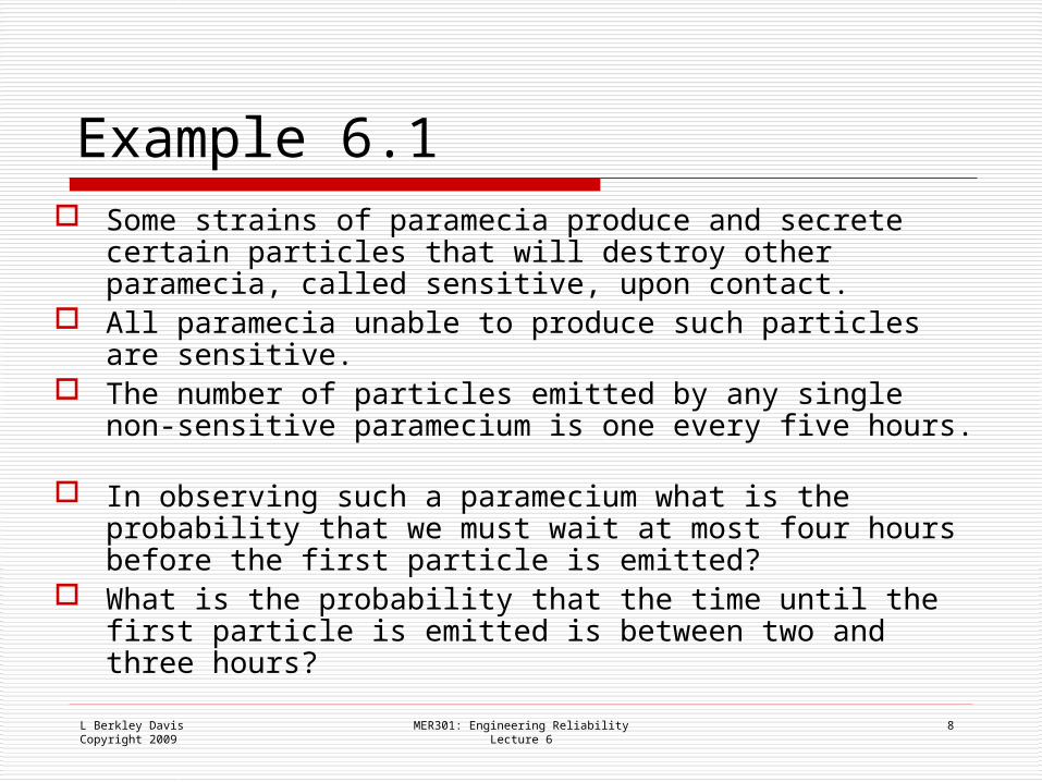
Example 6.1 Some strains of paramecia produce and secrete certain
particles that will destroy other paramecia, called sensitive, upon contact.
All paramecia unable to produce such particles are sensitive.
The number of particles emitted by any single non-sensitive paramecium is one every five hours.
In observing such a paramecium what is the probability that we must wait at most four hours before the first particle is emitted?
What is the probability that the time until the first particle is emitted is between two and three hours?
L Berkley DavisCopyright 2009
MER301: Engineering ReliabilityLecture 6
9
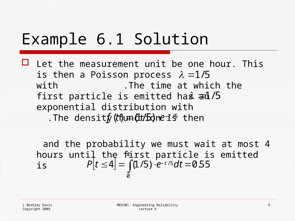
Example 6.1 Solution Let the measurement unit be one hour. This is then
a Poisson process with .The time at which the first particle is emitted has an exponential distribution with .The density function is then
and the probability we must wait at most 4 hours until the first particle is emitted is
5/1
5/1
5/)5/1()( tetf
55.0)5/1(44
0
5/ dtetP t
L Berkley DavisCopyright 2009
MER301: Engineering ReliabilityLecture 6
10
More than One Random Variable and Independence Most engineering design problems require that
multiple variables be dealt with in designing products Control variables “noise” variables
Independence implies that variation in one variable is not related to variation in another
L Berkley DavisCopyright 2009
MER301: Engineering ReliabilityLecture 6
11
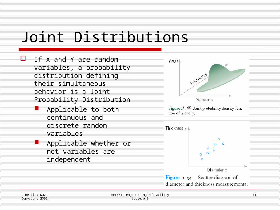
Joint Distributions If X and Y are random
variables, a probability distribution defining their simultaneous behavior is a Joint Probability Distribution Applicable to both
continuous and discrete random variables
Applicable whether or not variables are independent
3-39
3-40
L Berkley DavisCopyright 2009
MER301: Engineering ReliabilityLecture 6
12
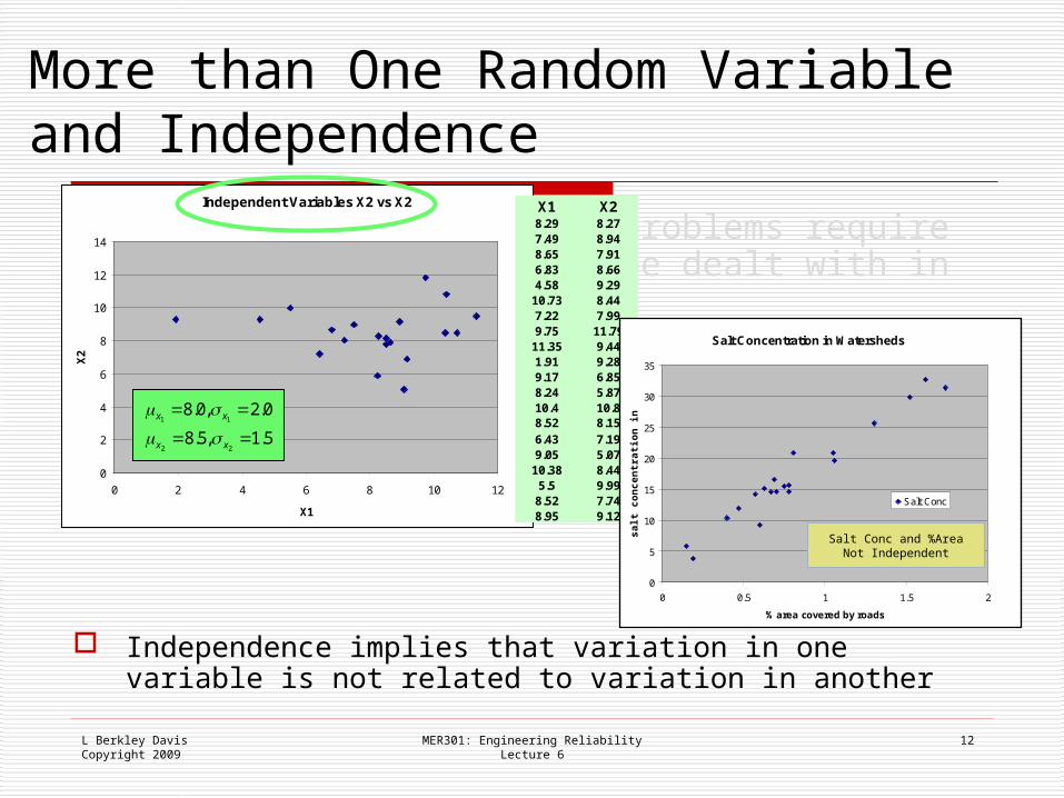
More than One Random Variable and Independence
Most engineering design problems require that multiple variables be dealt with in designing products Control variables “noise” variables
Independence implies that variation in one variable is not related to variation in another
Independent Variables X2 vs X2
0
2
4
6
8
10
12
14
0 2 4 6 8 10 12
X1
X2 X2
X1 X28.29 8.277.49 8.948.65 7.916.83 8.664.58 9.29
10.73 8.447.22 7.999.75 11.79
11.35 9.441.91 9.289.17 6.858.24 5.8710.4 10.88.52 8.156.43 7.199.05 5.07
10.38 8.445.5 9.99
8.52 7.748.95 9.12
5.1,5.8
0.2,0.8
22
11
xx
xx
Salt Concentration in Watersheds
0
5
10
15
20
25
30
35
0 0.5 1 1.5 2
% area covered by roads
salt
co
nce
ntr
atio
n i
n r
un
off
Salt Conc
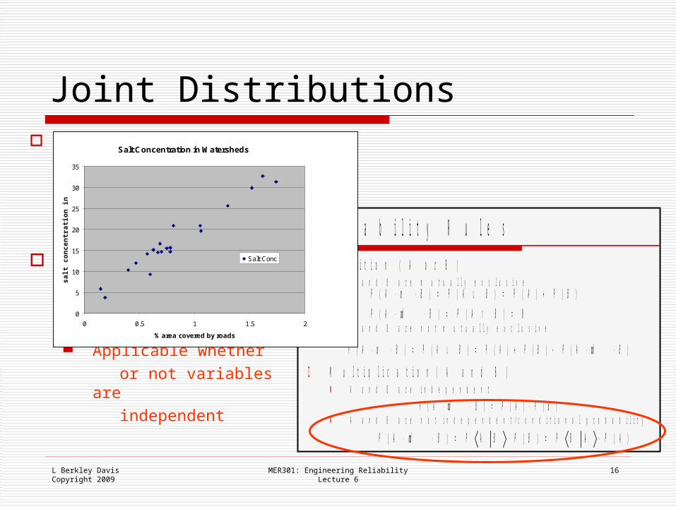
Salt Conc and %AreaNot Independent
L Berkley DavisCopyright 2009
MER301: Engineering ReliabilityLecture 6
13
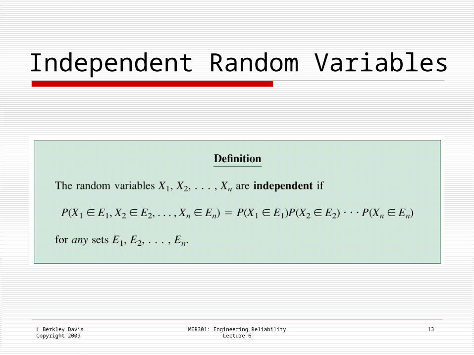
Independent Random Variables
L Berkley DavisCopyright 2009
U n i o n C o l l e g eM e c h a n i c a l E n g i n e e r i n g
M E R 3 0 1 : E n g i n e e r i n g R e l i a b i l i t yL e c t u r e 1
4 1
P r o b a b i l i t y R u l e s
A d d i t i o n ( A o r B ) A a n d B a r e m u t u a l l y e x c l u s i v e
A a n d B a r e n o t m u t u a l l y e x c l u s i v e
M u l t i p l i c a t i o n ( A a n d B ) A a n d B a r e i n d e p e n d e n t
A a n d B a r e n o t i n d e p e n d e n t / c o n d i t i o n a l p r o b a b i l i t y
)()()()()( BandAPBPAPBAPBorAP
0)()(
)()()()(
BAPBandAP
BPAPBAPBorAP
)()()( BPAPBandAP
)()()( APABPBPBAPBandAP
MER301: Engineering ReliabilityLecture 6
14
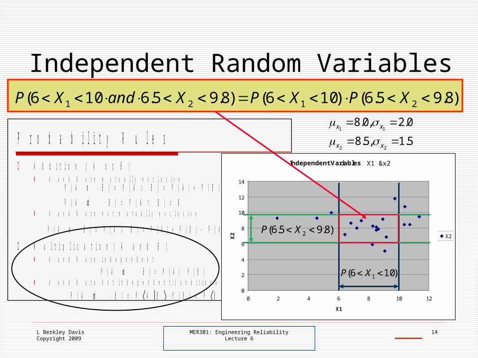
Independent Random Variables
Independent Variables X2 vs X2
0
2
4
6
8
10
12
14
0 2 4 6 8 10 12
X1
X2 X2
)8.95.6( 2 XP
)106( 1 XP
)8.95.6()106()8.95.6106( 2121 XPXPXandXP
X1 &x2
5.1,5.8
0.2,0.8
22
11
xx
xx
L Berkley DavisCopyright 2009
MER301: Engineering ReliabilityLecture 6
15
Union Coll egeMechanical Engi neeri ng
MER301: Engi neering ReliabilityLecture 16
Actual Defects
LSL USL
= Product Std. Dev.= Product Mean
LSL USL
Observed Defects
Measurement system variance
Product variance
Impact of Measurement System Variation on Variation in Experimental Data
22mactualobs
actual
actual
actual
obs observedobs
tmeasuremenm
actualact
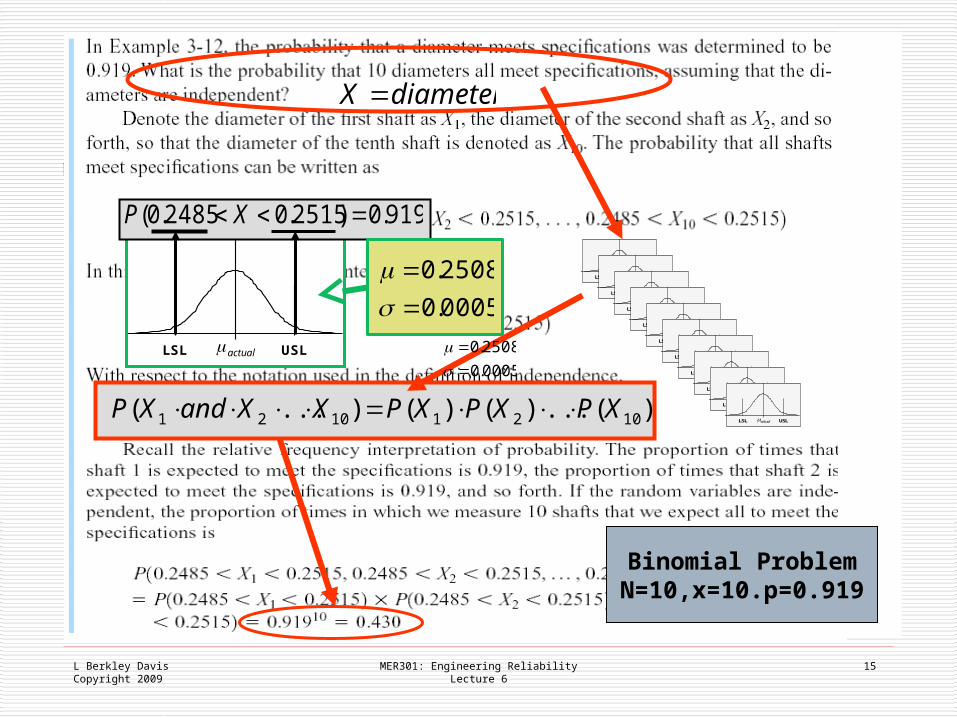
)(...)()()...( 10211021 XPXPXPXXandXP
diameterX
Unio n Col l eg eMec ha nic al E ngi ne eri ng
ME R30 1: E ngi ne erin g R el iabi l i tyLe ct ur e 1 6
Actual Defects
LSL USL
= Product Std. Dev.= Product Mean
LSL USL
Observed Defects
Measurement system variance
Product variance
Impact of Measurement System Variation on Variation in Experimental Data
22mactualobs
actual
actual
actual
obs observedobs
tmeasuremenm
actualact
919.0)2515.02485.0( XP
0005.0
2508.0
0005.0
2508.0
Binomial ProblemN=10,x=10.p=0.919
L Berkley DavisCopyright 2009
U n i o n C o l l e g eM e c h a n i c a l E n g i n e e r i n g
M E R 3 0 1 : E n g i n e e r i n g R e l i a b i l i t yL e c t u r e 1
4 1
P r o b a b i l i t y R u l e s
A d d i t i o n ( A o r B ) A a n d B a r e m u t u a l l y e x c l u s i v e
A a n d B a r e n o t m u t u a l l y e x c l u s i v e
M u l t i p l i c a t i o n ( A a n d B ) A a n d B a r e i n d e p e n d e n t
A a n d B a r e n o t i n d e p e n d e n t / c o n d i t i o n a l p r o b a b i l i t y
)()()()()( BandAPBPAPBAPBorAP
0)()(
)()()()(
BAPBandAP
BPAPBAPBorAP
)()()( BPAPBandAP
)()()( APABPBPBAPBandAP
MER301: Engineering ReliabilityLecture 6
16
Joint Distributions If X and Y are random
variables, a probability distribution defining their simultaneous behavior is a Joint Probability Distribution
Applicable to both continuous and discrete random variables Applicable whether or not variables are independent
Salt Concentration in Watersheds
0
5
10
15
20
25
30
35
0 0.5 1 1.5 2
% area covered by roads
salt
co
nce
ntr
atio
n i
n r
un
off
Salt Conc
L Berkley DavisCopyright 2009
MER301: Engineering ReliabilityLecture 6
17
Independence of Random Variables or Events
Concept of independent random variables/events underlies many statistical analysis methods
If Y=f(x1,x2,…xn) then the values y1,…yk obtained from k repetitions of an experiment are independent if and only if x1,…xn are random independent variables
L Berkley DavisCopyright 2009
MER301: Engineering ReliabilityLecture 6
18
Reliability Reliability Analysis quantifies whether or not a design
functions adequately for the required life when operating under the conditions for which it is designed- whether it… Meets Functional Requirements over Operating Life Achieves Design Life before Replacement/Repair Tolerates Needed range of Environmental Conditions
The objective of Reliability Analysis is to predict the probability of failure at a specific time t, number of cycles, etc Failure density function, f(t) Cumulative density function, F(t)=probability of failure at
time t Reliability function, R(t) = I-F(t)=probability of no failure at
time t
L Berkley DavisCopyright 2009
MER301: Engineering ReliabilityLecture 6
19
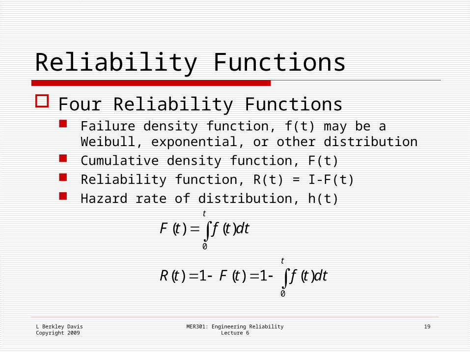
Reliability Functions
Four Reliability Functions Failure density function, f(t) may be a Weibull,
exponential, or other distribution Cumulative density function, F(t) Reliability function, R(t) = I-F(t) Hazard rate of distribution, h(t)
t
t
dttftFtR
dttftF
0
0
)(1)(1)(
)()(
L Berkley DavisCopyright 2009
MER301: Engineering ReliabilityLecture 6
20
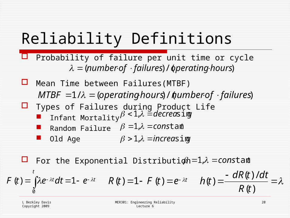
Reliability Definitions Probability of failure per unit time or cycle
Mean Time between Failures(MTBF)
Types of Failures during Product Life Infant Mortality Random Failure Old Age
For the Exponential Distribution
)/()( hoursoperatingfailuresofnumber
)/()(/1 failuresofnumberhoursoperatingMTBF
gincrea
tcons
gdecrea
sin,1
tan,1
sin,1
t
t
t edtetF 1)(0
tcons tan,1
tetFtR )(1)(
)(
/)()(
tR
dttdRth
L Berkley DavisCopyright 2009
failure rate for delta=1000X beta=0.5 beta=1 beta=2 beta=3 beta=40 0 0 0 0 0
10 0.095 0.01 0 0 050 0.2 0.049 0.002 0 0
100 0.271 0.095 0.01 0.001 0200 0.361 0.181 0.039 0.008 0.002500 0.507 0.393 0.221 0.118 0.061
1000 0.632 0.632 0.632 0.632 0.6322000 0.757 0.865 0.982 1 15000 0.893 0.993 1 1 1
10000 0.958 1 1 1 1
MER301: Engineering ReliabilityLecture 6
21
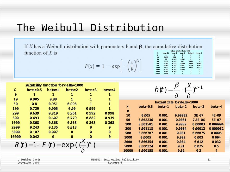
The Weibull Distribution
1)()(
x
th
))(exp()(1)(
x
tFtR
reliability function for delta=1000X beta=0.5 beta=1 beta=2 beta=3 beta=40 1 1 1 1 1
10 0.905 0.99 1 1 150 0.8 0.951 0.998 1 1
100 0.729 0.905 0.99 0.999 1200 0.639 0.819 0.961 0.992 0.998500 0.493 0.607 0.779 0.882 0.939
1000 0.368 0.368 0.368 0.368 0.3682000 0.243 0.135 0.018 0 05000 0.107 0.007 0 0 0
10000 0.042 0 0 0 0
hazard rate for delta=1000X beta=0.5 beta=1 beta=2 beta=3 beta=40
10 0.005 0.001 0.00002 3E-07 4E-0950 0.002236 0.001 0.0001 7.5E-06 5E-07
100 0.001581 0.001 0.0002 0.00003 0.000004200 0.001118 0.001 0.0004 0.00012 0.000032500 0.000707 0.001 0.001 0.00075 0.0005
1000 0.0005 0.001 0.002 0.003 0.0042000 0.000354 0.001 0.004 0.012 0.0325000 0.000224 0.001 0.01 0.075 0.5
10000 0.000158 0.001 0.02 0.3 4
L Berkley DavisCopyright 2009
MER301: Engineering ReliabilityLecture 6
22
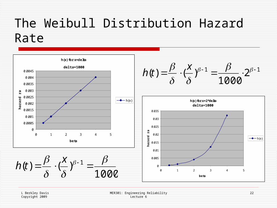
The Weibull Distribution Hazard Rate
h(x) for x=delta
0
0.0005
0.001
0.0015
0.002
0.0025
0.003
0.0035
0.004
0.0045
0 1 2 3 4 5
beta
haz
ard
rat
e
h(x) h(x) for x=2*delta
0
0.005
0.01
0.015
0.02
0.025
0.03
0.035
0 1 2 3 4 5
beta
haz
ard
rat
e
h(x)
11 21000
)()(
xth
1000)()( 1
x
th
delta=1000
delta=1000
L Berkley DavisCopyright 2009
MER301: Engineering ReliabilityLecture 6
23
Reliability What kinds of Systems require reliability analysis?
Individual components(gas turbine compressor blades) or Assemblies(motors, pumps,valves, instruments)
Software (firmware, distributed controls code,plant level controls code, applications code)
Systems comprising multiple components or assemblies or software(gas turbine gas fuel system)
What are the methods used in reliability analysis? Testing to establish capability of components, assemblies,
systems, software Reliability Block Diagrams to model entire Systems Analysis of Reliability Models to assess performance Field Data gathering to validate models
L Berkley DavisCopyright 2009
MER301: Engineering ReliabilityLecture 6
24
Reliability Testing Reliability Tests are conducted to establish the tolerance
of components,assemblies, and systems to environmental factors Dust, dirt,chemical contaminants Vibration Operating Temperature range Ambient Temperature range Moisture,humidity
Reliability Tests are typically conducted by exercising the system Subjecting systems to environmental stress testing Exercising the system through a number of operational
cycles equivalent to product life requirements Conducting HALT tests to get data more quickly
L Berkley DavisCopyright 2009
MER301: Engineering ReliabilityLecture 6
25
Reliability Analysis Most designs consist of multiple subsystems,
assemblies,and components each with it own probability of failing or not Probability of overall system functioning is a
function of subsystem characteristics The way subsystems are arranged in a system
determines overall reliability
L Berkley DavisCopyright 2009
MER301: Engineering ReliabilityLecture 6
26
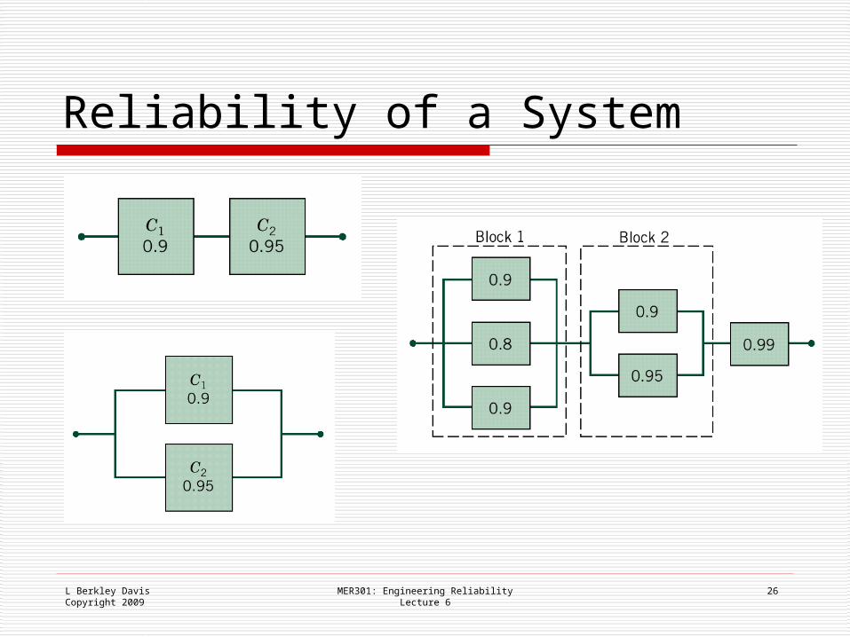
Reliability of a System
L Berkley DavisCopyright 2009
Venn Diagram
MER301: Engineering ReliabilityLecture 6
27
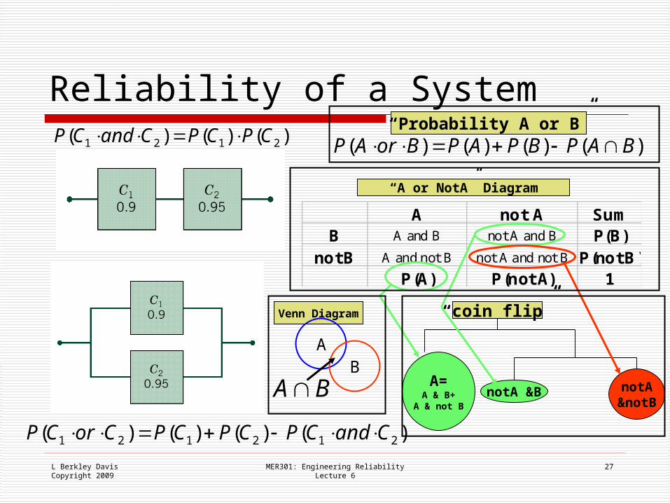
Reliability of a System)()()( 2121 CPCPCandCP
)()()()( 212121 CandCPCPCPCorCP
A not A SumB A and B not A and B P(B)
not B A and not B not A and not B P(not B)P(A) P(not A) 1
AB
BA
)()()()( BAPBPAPBorAP
A=A & B+
A & not BnotA &B notA
¬B
“coin flip”
“A or NotA” Diagram
“Probability A or B”
L Berkley DavisCopyright 2009
MER301: Engineering ReliabilityLecture 6
28
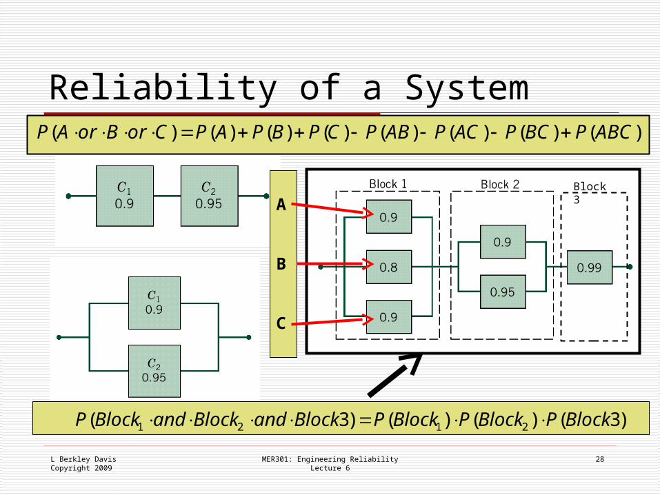
Reliability of a System
)3()()()3( 2121 BlockPBlockPBlockPBlockandBlockandBlockP
)()()()()()()()( ABCPBCPACPABPCPBPAPCorBorAP
Block 3A
B
C
L Berkley DavisCopyright 2009
MER301: Engineering ReliabilityLecture 6
29
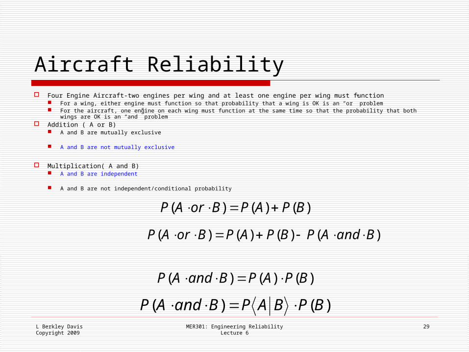
Aircraft Reliability Four Engine Aircraft-two engines per wing and at least one engine per wing must function
For a wing, either engine must function so that probability that a wing is OK is an “or” problem For the aircraft, one engine on each wing must function at the same time so that the probability that both wings are OK is an
“and” problem Addition ( A or B)
A and B are mutually exclusive
A and B are not mutually exclusive
Multiplication( A and B) A and B are independent
A and B are not independent/conditional probability
)()()()( BandAPBPAPBorAP
)()()( BPAPBorAP
)()()( BPAPBandAP
)()( BPBAPBandAP
L Berkley DavisCopyright 2009
MER301: Engineering ReliabilityLecture 6
30
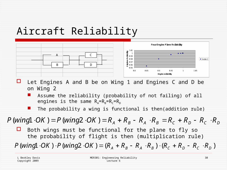
Aircraft Reliability
A
B D
C
Let Engines A and B be on Wing 1 and Engines C and D be on Wing 2 Assume the reliability (probability of not failing) of all engines is the
same RA=RB=RC=RD
The probability a wing is functional is then(addition rule)
Both wings must be functional for the plane to fly so the probability of flight is then (multiplication rule)
DCDCBABA RRRRRRRROKwingPOKwingP )2()1(
)()()2()1( DCDCBABA RRRRRRRROKwingPOKwingP
Four Engine Plane Reliability
0.95
0.96
0.97
0.98
0.99
1
1.01
0.8 0.85 0.9 0.95 1 1.05
Engine reliability
Air
pla
ne
Re
liab
ility
Series1
L Berkley DavisCopyright 2009
MER301: Engineering ReliabilityLecture 6
31
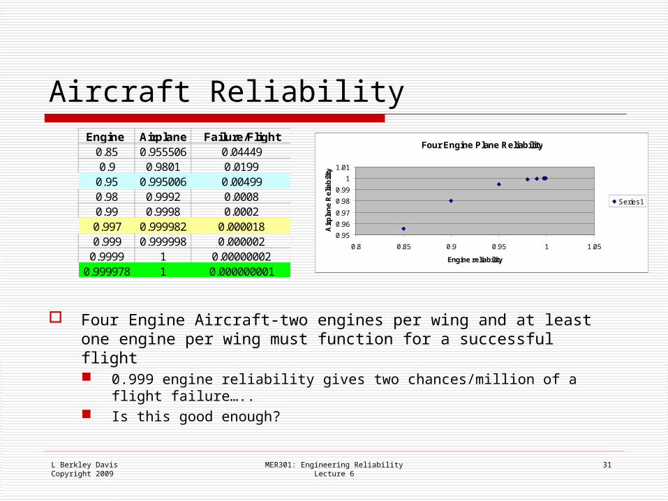
Aircraft ReliabilityEngine Airplane Failure/Flight
0.85 0.955506 0.044490.9 0.9801 0.0199
0.95 0.995006 0.004990.98 0.9992 0.00080.99 0.9998 0.00020.997 0.999982 0.0000180.999 0.999998 0.000002
0.9999 1 0.000000020.999978 1 0.000000001
Four Engine Plane Reliability
0.95
0.96
0.97
0.98
0.99
1
1.01
0.8 0.85 0.9 0.95 1 1.05
Engine reliability
Air
pla
ne
Re
liab
ility
Series1
Four Engine Aircraft-two engines per wing and at least one engine per wing must function for a successful flight 0.999 engine reliability gives two chances/million of a flight
failure….. Is this good enough?
L Berkley DavisCopyright 2009
MER301: Engineering ReliabilityLecture 6
32
Aircraft Reliability
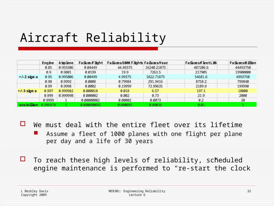
Engine Airplane Failure/Flight Failures/1000 Flights Failures/Year Failures/Fleet Life Failures/Billion0.85 0.955506 0.04449 44.49375 16240.21875 487206.6 444937500.9 0.9801 0.0199 19.9 7263.5 217905 19900000
+/- 2 sigma 0.95 0.995006 0.00499 4.99375 1822.71875 54681.6 49937500.98 0.9992 0.0008 0.79984 291.9416 8758.2 7998400.99 0.9998 0.0002 0.19999 72.99635 2189.9 199990
+/- 3 sigma 0.997 0.999982 0.000018 0.018 6.57 197.1 180000.999 0.999998 0.000002 0.002 0.73 21.9 2000
0.9999 1 0.00000002 0.00002 0.0073 0.2 20one/billion 0.999978 1 0.000000001 0.000001 0.00036 0.01 1
We must deal with the entire fleet over its lifetime Assume a fleet of 1000 planes with one flight per plane per day
and a life of 30 years
To reach these high levels of reliability, scheduled engine maintenance is performed to “re-start”the clock
L Berkley DavisCopyright 2009
MER301: Engineering ReliabilityLecture 6
33
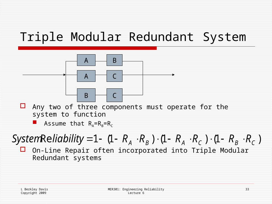
Triple Modular Redundant System
Any two of three components must operate for the system to function Assume that RA=RB=RC
On-Line Repair often incorporated into Triple Modular Redundant systems
B
C
C
A
B
A
)1()1()1(1Re CBCABA RRRRRRliabilitySystem
L Berkley DavisCopyright 2009
MER301: Engineering ReliabilityLecture 6
34
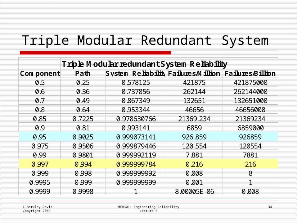
Triple Modular Redundant System
Triple Modular redundant System ReliabilityComponent Path System Reliability Failures/Million Failures/Billion
0.5 0.25 0.578125 421875 4218750000.6 0.36 0.737856 262144 2621440000.7 0.49 0.867349 132651 1326510000.8 0.64 0.953344 46656 46656000
0.85 0.7225 0.978630766 21369.234 213692340.9 0.81 0.993141 6859 6859000
0.95 0.9025 0.999073141 926.859 9268590.975 0.9506 0.999879446 120.554 1205540.99 0.9801 0.999992119 7.881 78810.997 0.994 0.999999784 0.216 2160.999 0.998 0.999999992 0.008 8
0.9995 0.999 0.999999999 0.001 10.9999 0.9998 1 8.00005E-06 0.008

L Berkley DavisCopyright 2009
MER301: Engineering ReliabilityLecture 6
35
Summary
Exponential Distribution
Independence
Joint Distributions
Reliability