Kuridze, D. et al. (2015) H± line profile asymmetries and the chromospheric flare velocity field. Astrophysical Journal, 813(2), 125. There may be differences between this version and the published version. You are advised to consult the publisher’s version if you wish to cite from it.

http://eprints.gla.ac.uk/111123/ Deposited on: 21 December 2015

Enlighten – Research publications by members of the University of Glasgow http://eprints.gla.ac.uk

Draft version October 8, 2015Preprint typeset using LATEX style emulateapj v. 12/16/11

Hα LINE PROFILE ASYMMETRIES AND THE CHROMOSPHERIC FLARE VELOCITY FIELD

D. Kuridze1,5, M. Mathioudakis1, P. J. A. Simoes2, L. Rouppe van der Voort2, M. Carlsson3, S. Jafarzadeh3, J. C. Allred4, A. F. Kowalski4,M. Kennedy1, L. Fletcher2, D. Graham 6 & F. P. Keenan1

1Astrophysics Research Centre, School of Mathematics and Physics, Queen’s University Belfast, BT7 1NN, Northern Ireland, UK.2SUPA School of Physics and Astronomy, University of Glasgow, Glasgow G12 8QQ, U. K.

3Institute of Theoretical Astrophysics, University of Oslo, P.O. Box 1029 Blindern, N-0315 Oslo, Norway.4 NASA/Goddard Space Flight Center, Code 671, Greenbelt, MD 20771.

5 Abastumani Astrophysical Observatory at Ilia State University, 3/5 Cholokashvili avenue, 0162 Tbilisi, Georgia, and6 INAF-Ossevatorio Astrofisico di Arcetri, I-50125 Firenze, Italy.

(Dated: received / accepted)Draft version October 8, 2015

ABSTRACTThe asymmetries observed in the line profiles of solar flares can provide important diagnostics of the propertiesand dynamics of the flaring atmosphere. In this paper the evolution of the Hα and Ca ii 8542 Å lines are studiedusing high spatial, temporal and spectral resolution ground-based observations of an M1.1 flare obtained withthe Swedish 1-m Solar Telescope. The temporal evolution of the Hα line profiles from the flare kernel showsexcess emission in the red wing (red asymmetry) before flare maximum, and excess in the blue wing (blueasymmetry) after maximum. However, the Ca ii 8542 Å line does not follow the same pattern, showing onlya weak red asymmetry during the flare. RADYN simulations are used to synthesise spectral line profiles forthe flaring atmosphere, and good agreement is found with the observations. We show that the red asymmetryobserved in Hα is not necessarily associated with plasma downflows, and the blue asymmetry may not berelated to plasma upflows. Indeed, we conclude that the steep velocity gradients in the flaring chromospheremodifies the wavelength of the central reversal in the Hα line profile. The shift in the wavelength of maximumopacity to shorter and longer wavelengths generates the red and blue asymmetries, respectively.

1. INTRODUCTION

It is widely accepted that the vast majority of the solar flareradiative energy originates in the photosphere and chromo-sphere. The chromospheric radiation is dominated by hy-drogen, calcium and magnesium lines, plus hydrogen con-tinua, providing vital diagnostics on energy deposition ratesin the lower atmosphere. One of the main characteristics ofthe flaring chromosphere is the centrally reversed Hα emis-sion line profile with asymmetric red and blue wings (see thereview by Berlicki 2007). Earlier observations have shownthat the red asymmetry in the Hα line profile is more typi-cal and is observed frequently during the impulsive phase ofthe flare (Svestka 1976; Tang 1983; Ichimoto & Kurokawa1984; Wulser & Marti 1989; Falchi et al. 1997). High resolu-tion spectroscopy indicates that the red asymmetry dominatesover the ribbons during the flare (Asai et al. 2012; Deng et al.2013; Huang et al. 2014). However, blue asymmetries havealso been reported and these occur mainly in the early stagesof the flare (Svestka et al. 1962; Severny 1968; Heinzel et al.1994; Mein et al. 1997; Yu & Gan 2006). Furthermore, blueand red asymmetries at different positions in the same flareribbon, and the reversal of asymmetry at a same position inthe ribbon have also been reported (Canfield et al. 1990a; Jiet al. 1994; Mein et al. 1997). The Ca ii 8542 Å line profile,which goes into full emission during the flare, is also asym-metric (Li et al. 2007), but its asymmetric properties do notnecessary coincide with those detected simultaneously in Hα(Mein et al. 1997).

Despite a number of attempts to explain the observed asym-metries, their exact nature remains unclear. Theoretical lineprofiles based on static models of flare chromospheres do notshow asymmetric signatures (Canfield & Gayley 1984; Fanget al. 1993; Cheng et al. 2006). This suggests that the asym-

metries are related to the velocity field in the flaring atmo-sphere.

The red asymmetries observed in chromospheric lines dur-ing flares are usually attributed to the downflow of coolplasmas in the flaring atmosphere, a process also known aschromospheric condensation (Ichimoto & Kurokawa 1984;Wulser & Marti 1989; de la Beaujardiere et al. 1992). Asthe flare energy is deposited in the chromosphere, a strongevaporation of the heated plasma occurs (e.g. Neupert 1968;Fisher et al. 1985; Graham & Cauzzi 2015). Conservation ofmomentum requires the formation of a downflow in the formof chromospheric condensation (Ichimoto & Kurokawa 1984;Canfield et al. 1990b; Milligan & Dennis 2009; Hudson 2011;Kerr et al. 2015). If the downflow occurs in the upper chromo-sphere, its effect would be a red-wing absorption which canlead to a blue asymmetry in the line profile (Gan et al. 1993;Heinzel et al. 1994). Ding & Fang (1996) have shown thatboth red and blue asymmetries in the Hα line can be causedby downward moving plasma at different heights in the solarchromosphere. This blue asymmetry has also been interpretedin terms of chromospheric evaporation and filament activation(Canfield et al. 1990a; Huang et al. 2014).

Abbett & Hawley (1999) computed time-dependent Hα andCa ii K line profiles with the radiative-hydrodynamic code(RADYN; Carlsson & Stein 1997) for weak (F10) and strong(F11) flare runs, and showed that asymmetries could be pro-duced by the strong velocity gradients generated during theflare. The velocity gradients create differences in the opacitybetween the red and blue wings of Hα, and the sign of the gra-dient determines whether the asymmetric emission appears tothe blue or red side of the line profile. This process was firstreported in the pioneering work of Carlsson & Stein (1997),who studied the effects of acoustic shocks on the formation of

arX

iv:1

510.

0187

7v1

[as

tro-

ph.S

R]

7 O

ct 2

015

2

AIA 94 Å

0 10 20 30 40 500

10

20

30

40

50

arcs

ecHα − 1.4 Å

0 10 20 30 40 500

10

20

30

40

50

Hα (core) 6562 Å

0 10 20 30 40 500

10

20

30

40

50

Hα + 1.4 Å

0 10 20 30 40 500

10

20

30

40

50

Fe I 6302 − 0.048 Å (running difference image)

0 10 20 30 40 50arcsec

0

10

20

30

40

50

arcs

ec

Ca II 8542 − 0.8 Å

0 10 20 30 40 50arcsec

0

10

20

30

40

50

Ca II 8542 (core) Å

0 10 20 30 40 50arcsec

0

10

20

30

40

50

Ca II 8542 + 0.8 Å

0 10 20 30 40 50arcsec

0

10

20

30

40

50

16:55:25−16:55:02 UT

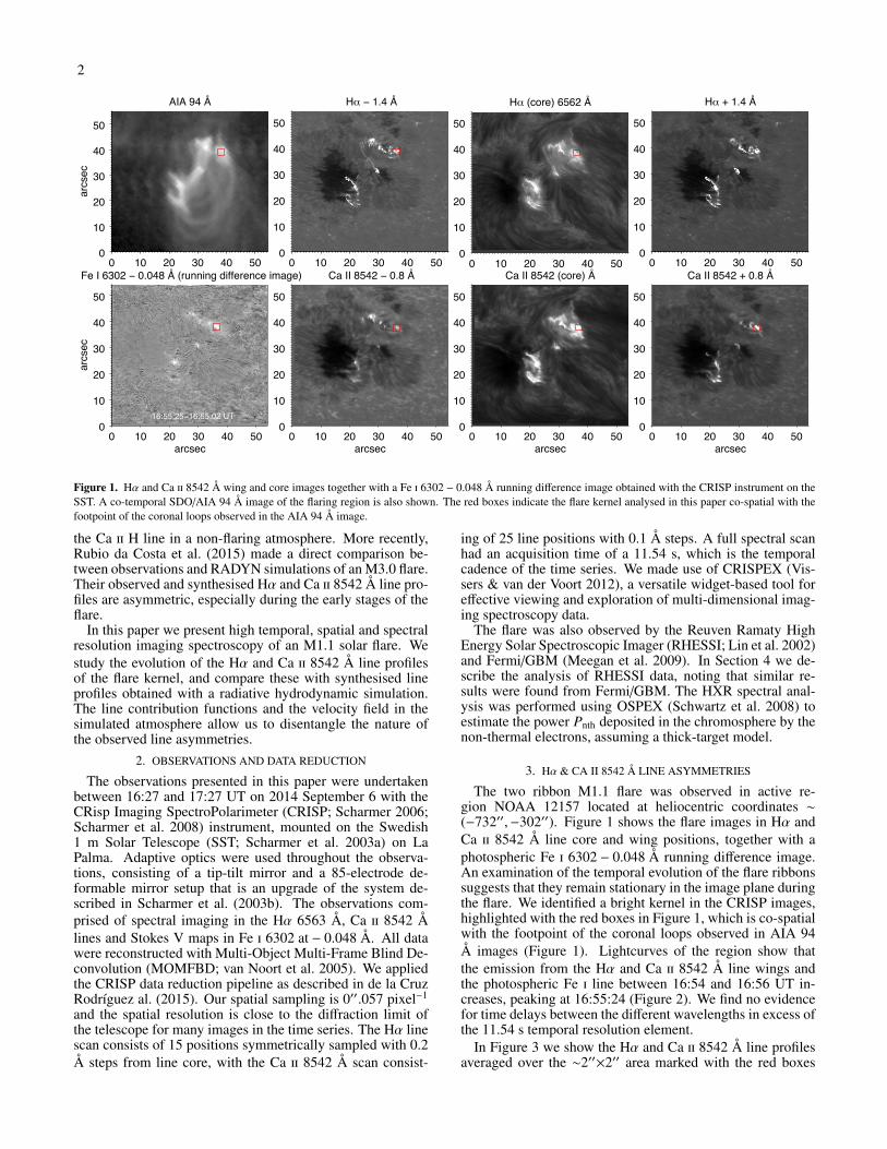
Figure 1. Hα and Ca ii 8542 Å wing and core images together with a Fe i 6302 − 0.048 Å running difference image obtained with the CRISP instrument on theSST. A co-temporal SDO/AIA 94 Å image of the flaring region is also shown. The red boxes indicate the flare kernel analysed in this paper co-spatial with thefootpoint of the coronal loops observed in the AIA 94 Å image.

the Ca ii H line in a non-flaring atmosphere. More recently,Rubio da Costa et al. (2015) made a direct comparison be-tween observations and RADYN simulations of an M3.0 flare.Their observed and synthesised Hα and Ca ii 8542 Å line pro-files are asymmetric, especially during the early stages of theflare.

In this paper we present high temporal, spatial and spectralresolution imaging spectroscopy of an M1.1 solar flare. Westudy the evolution of the Hα and Ca ii 8542 Å line profilesof the flare kernel, and compare these with synthesised lineprofiles obtained with a radiative hydrodynamic simulation.The line contribution functions and the velocity field in thesimulated atmosphere allow us to disentangle the nature ofthe observed line asymmetries.

2. OBSERVATIONS AND DATA REDUCTION

The observations presented in this paper were undertakenbetween 16:27 and 17:27 UT on 2014 September 6 with theCRisp Imaging SpectroPolarimeter (CRISP; Scharmer 2006;Scharmer et al. 2008) instrument, mounted on the Swedish1 m Solar Telescope (SST; Scharmer et al. 2003a) on LaPalma. Adaptive optics were used throughout the observa-tions, consisting of a tip-tilt mirror and a 85-electrode de-formable mirror setup that is an upgrade of the system de-scribed in Scharmer et al. (2003b). The observations com-prised of spectral imaging in the Hα 6563 Å, Ca ii 8542 Ålines and Stokes V maps in Fe i 6302 at − 0.048 Å. All datawere reconstructed with Multi-Object Multi-Frame Blind De-convolution (MOMFBD; van Noort et al. 2005). We appliedthe CRISP data reduction pipeline as described in de la CruzRodrıguez al. (2015). Our spatial sampling is 0′′.057 pixel−1

and the spatial resolution is close to the diffraction limit ofthe telescope for many images in the time series. The Hα linescan consists of 15 positions symmetrically sampled with 0.2Å steps from line core, with the Ca ii 8542 Å scan consist-

ing of 25 line positions with 0.1 Å steps. A full spectral scanhad an acquisition time of a 11.54 s, which is the temporalcadence of the time series. We made use of CRISPEX (Vis-sers & van der Voort 2012), a versatile widget-based tool foreffective viewing and exploration of multi-dimensional imag-ing spectroscopy data.

The flare was also observed by the Reuven Ramaty HighEnergy Solar Spectroscopic Imager (RHESSI; Lin et al. 2002)and Fermi/GBM (Meegan et al. 2009). In Section 4 we de-scribe the analysis of RHESSI data, noting that similar re-sults were found from Fermi/GBM. The HXR spectral anal-ysis was performed using OSPEX (Schwartz et al. 2008) toestimate the power Pnth deposited in the chromosphere by thenon-thermal electrons, assuming a thick-target model.

3. Hα & CA II 8542 Å LINE ASYMMETRIES

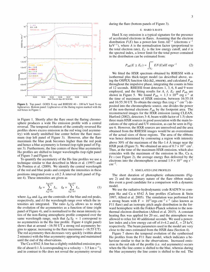
The two ribbon M1.1 flare was observed in active re-gion NOAA 12157 located at heliocentric coordinates ∼(−732′′,−302′′). Figure 1 shows the flare images in Hα andCa ii 8542 Å line core and wing positions, together with aphotospheric Fe i 6302 − 0.048 Å running difference image.An examination of the temporal evolution of the flare ribbonssuggests that they remain stationary in the image plane duringthe flare. We identified a bright kernel in the CRISP images,highlighted with the red boxes in Figure 1, which is co-spatialwith the footpoint of the coronal loops observed in AIA 94Å images (Figure 1). Lightcurves of the region show thatthe emission from the Hα and Ca ii 8542 Å line wings andthe photospheric Fe i line between 16:54 and 16:56 UT in-creases, peaking at 16:55:24 (Figure 2). We find no evidencefor time delays between the different wavelengths in excess ofthe 11.54 s temporal resolution element.

In Figure 3 we show the Hα and Ca ii 8542 Å line profilesaveraged over the ∼2′′×2′′ area marked with the red boxes

3

10−8

10−7

10−6

10−5

GO

ES fl

ux, W

m−2

10

100

1000

10000

RHES

SI 4

0−10

0 ke

V co

unts

16:53 16:54 16:55 16:56 16:57 16:58 16:59Start Time (6−Sep−09 16:52:06)

0

2.0×103

4.0×103

6.0×103

8.0×103

1.0×104

1.2×104

Inte

nsity

1 − 8 Å

RHESSI 40 − 100 keV

Fe 6302 − 0.048 ÅHα − 1.4 ÅHα 6563 ÅHα + 1.4 ÅCa II 8543 − 0.8 ÅCa II 8543 ÅCa II 8543 + 0.8 Å

0.5 − 4 Å

Fe 6302−0.048 ÅHalpha−1.4 ÅHalpha 6563 ÅHalpha+1.4 ÅCa II 8543 − 0.8 ÅCa II 8543 ÅCa II 8543 + 0.8 Å

Fe 6302−0.048 ÅHalpha−1.4 ÅHalpha 6563 ÅHalpha+1.4 ÅCa II 8543 − 0.8 ÅCa II 8543 ÅCa II 8543 + 0.8 Å

Fe 6302−0.048 ÅHalpha−1.4 ÅHalpha 6563 ÅHalpha+1.4 ÅCa II 8543 − 0.8 ÅCa II 8543 ÅCa II 8543 + 0.8 Å

Fe 6302−0.048 ÅHalpha−1.4 ÅHalpha 6563 ÅHalpha+1.4 ÅCa II 8543 − 0.8 Å

Ca II 8543 + 0.8 Å

Figure 2. Top panel: GOES X-ray and RHESSI 40 − 100 keV hard X-raylightcurves. Bottom panel: Lightcurves of the flaring region marked with thered boxes in Figure 1.

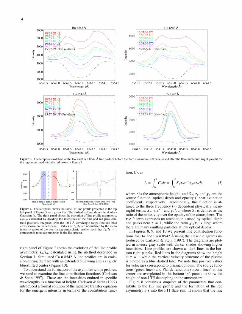
in Figure 1. Shortly after the flare onset the flaring chromo-sphere produces a wide Hα emission profile with a centralreversal. The temporal evolution of the centrally reversed Hαprofiles shows excess emission in the red wing (red asymme-try) with nearly unshifted line center before the flare maxi-mum (top left panel of Figure 3). However, after the flaremaximum the blue peak becomes higher than the red peakand hence a blue asymmetry is formed (top right panel of Fig-ure 3). Furthermore, the line centers of these blue asymmetricHα profiles are shifted to longer wavelengths (top right panelof Figure 3 and Figure 4).

To quantify the asymmetry of the Hα line profiles we use atechnique similar to that described in Mein et al. (1997) andDe Pontieu et al. (2009). We identify the central wavelengthof the red and blue peaks and compute the intensities in thesepositions integrated over a ±0.2 Å interval (left panel of Fig-ure 4). These intensities are given as

IB =

λ0B+δλ∑λ0B−δλ

Iλ, IR =

λ0R+δλ∑λ0R−δλ

Iλ, (1)

where λ0B and λ0R are the centroids of the blue and red peaks,respectively, and δλ the wavelength range over which the in-tensities are integrated. The ratio IB/IR allows us to studythe evolution of the asymmetries as a function of time (rightpanel of Figure 4), and is normalised to the mean intensity ra-tios of the non-flaring atmospheric profile computed over thesame wavelength range, such that IB/IR ≈ 1 correspond tono asymmetries in the Hα line profile. Figure 4 (right panel)shows that at around ∼16:50 UT a strong red asymmetry be-gins to appear, increasing to the flare maximum (∼16:55 UT).The red asymmetry then decreases very quickly (within about2 minutes) with the blue asymmetry appearing and maintaineduntil the end of the observations.

The Ca ii 8542 Å line has a slightly redshifted emission pro-file of about 0.1 Å (corresponding to a velocity ∼ 3.5 km s−1),and in contrast to Hα does not reveal the asymmetry reversal

during the flare (bottom panels of Figure 3).

4. HARD X-RAYS

Hard X-ray emission is a typical signature for the presenceof accelerated electrons in flares. Assuming that the electrondistribution F(E) has a power-law form AE−δ (electrons s−1

keV−1), where A is the normalisation factor (proportional tothe total electron rate), EC is the low energy cutoff, and δ isthe spectral index, a lower limit for the total power containedin the distribution can be estimated from:

Pnth(E ≥ EC) =

∫ ∞EC

EF(E)dE ergs−1 (2)

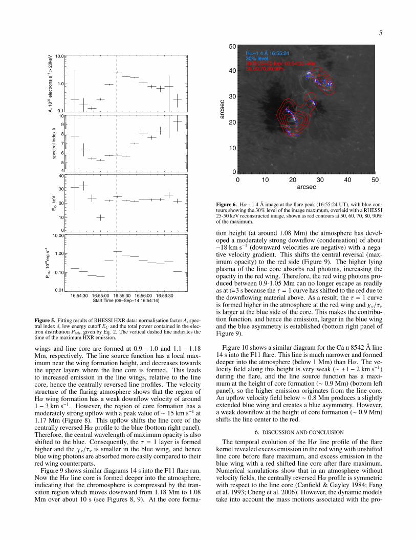
We fitted the HXR spectrum obtained by RHESSI with aisothermal plus thick-target model (as described above, us-ing the OSPEX function thick2_vnorm), and calculated Pnththroughout the impulsive phase, integrating the counts in binsof 12 seconds. RHESSI front detectors 1, 3, 6, 8 and 9 wereemployed, and the fitting results for A, δ, EC and Pnth areshown in Figure 5. We found Pnth ≈ 1.3 × 1028 erg s−1 atthe time of maximum of HXR emission, between 16:55:18and 16:55:30 UT. To obtain the energy flux (erg s−1 cm−2) de-posited into the chromospheric source, one divides the powerof the non-thermal electrons Pnth by the footpoint area. Thereconstructed images for the HXR emission (using CLEAN,Hurford (2002), detectors 3–8, beam width factor of 1.5) showthree main HXR sources in good association with the main lo-cations of the optical and UV emission, as can be seen in Fig-ure 6. However, the HXR sources are unresolved and the areaobtained from the RHESSI images would be an overestimateof the actual sizes of those regions. The area of the ribbonswas hence determined by contouring a region with intensityabove 30% of the maximum of the Hα-1.4 Å image near theHXR peak (Figure 5). We obtained an area of 0.7× 1017 cm2.Thus, at the time of the maximum HXR emission, which alsocoincides with the maximum of the emission in Hα, Ca ii,Fe i (see Figure 2), the average energy flux delivered by theelectrons into the chromosphere is around 1.9 × 1011 erg s−1

cm−2.

5. SIMULATED LINE PROFILES

The short duration of photospheric enhancements (Fig-ure 2) and the stationary nature of the flare ribbon makesthis event a good candidate for a comparison with a dynamicmodel.

We use the radiative-hydrodynamic code RADYN to com-pute Hα and Ca ii 8542 Å line profiles (Carlsson & Stein1997; Allred et al. 2005). The simulation was performed fora strong beam with F = 1011ergs cm−2 s−1 (also known asF11 flare) and an isotropic pitch angle distribution in the for-ward hemisphere with the Fokker-Planck solution to the non-thermal electron distribution (Allred et al. 2015). A constantheating flux was applied for 20 sec, and the atmosphere wasallowed to relax for 40 additional seconds. We used a power-law index and a low energy cut-off of δ=4.2 and Ec = 25 keV,respectively. The beam parameters used in the model are veryclose to the ones estimated from the HXR data (Section 4).

Figure 7 shows the temporal evolution of the synthesisedHα profiles from the F11 flare model, which indicates a be-haviour similar to that in the observations. Increased emis-sion in the red side of the profile (i.e. red asymmetry) occurswhen the Hα line centre is shifted to the blue, whereas duringthe blue asymmetry the line centre is shifted to the red. The

4

6561.5 6562.0 6562.5 6563.0 6563.5 6564.0 6564.5Wavelength (Å)

1000

2000

3000

4000

5000

6000

7000In

tens

ity

15:27:29 UT (Pre−flare)

Hα 6563 Å16:54:50 UT16:54:27 UT16:53:41 UT16:53:18 UT16:52:43 UT16:51:46 UT

6561.5 6562.0 6562.5 6563.0 6563.5 6564.0 6564.5Wavelength (Å)

2000

4000

6000

8000

Inte

nsity

15:27:29 UT (Pre−flare)

Hα 6563 Å16:55:36 UT16:56:22 UT16:56:45 UT16:57:31 UT16:58:36 UT16:59:29 UT

8540.5 8541.0 8541.5 8542.0 8542.5 8543.0 8543.5Wavelength (Å)

1000

2000

3000

4000

Inte

nsity

15:27:29 UT (Pre−flare)

Ca 8542 Å16:54:50 UT16:54:27 UT16:53:41 UT16:53:18 UT16:52:43 UT16:51:46 UT

8540.5 8541.0 8541.5 8542.0 8542.5 8543.0 8543.5Wavelength (Å)

1000

2000

3000

4000

5000

Inte

nsity

15:27:29 UT (Pre−flare)

Ca 8542 Å16:55:36 UT16:56:22 UT16:56:45 UT16:57:31 UT16:58:36 UT16:59:29 UT

Figure 3. The temporal evolution of the Hα and Ca ii 8542 Å line profiles before the flare maximum (left panels) and after the flare maximum (right panels) forthe region outlined with the red boxes in Figure 1.

6562.0 6562.5 6563.0 6563.5 6564.0Wavelength (Å)

2000

3000

4000

5000

6000

Inte

nsity

16:10 16:20 16:30 16:40 16:50 17:00 17:10 17:20Start Time (6-Sep-09 16:06:06)

0.8

0.9

1.0

1.1

1.2

I B/I R

Figure 4. The left panel shows the same Hα line profile presented in the topleft panel of Figure 3 with green line. The dashed red line shows the double-Gaussian fit. The right panel shows the evolution of line profile asymmetry,IB/IR, calculated by dividing the intensities of the blue and red peak cen-troid positions integrated over the ±0.2 Å wavelength range (red and blueareas shown on the left panel). Values of IB/IR are normalised by the meanintensity ratios of the non-flaring atmospheric profile, such that IB/IR ≈ 1corresponds to no asymmetries in the Hα spectra.

right panel of Figure 7 shows the evolution of the line profileasymmetry, IB/IR, calculated using the method described inSection 3. Simulated Ca ii 8542 Å line profiles are in emis-sion during the flare with an extended blue wing and a slightlyblueshifted center (Figure 10).

To understand the formation of the asymmetric line profiles,we need to examine the line contribution functions (Carlsson& Stein 1997). These are the intensities emitted in specificwavelengths as a function of height. Carlsson & Stein (1997)introduced a formal solution of the radiative transfer equationfor the emergent intensity in terms of the contribution func-

tion, CI , as

Iν =

∫ z

z0

CIdz =

∫ z

z0

S ντνe−τνχν/τνdz, (3)

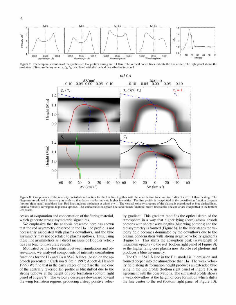
where z is the atmospheric height, and S ν, τν and χν are thesource function, optical depth and opacity (linear extinctioncoefficient), respectively. Traditionally, this function is at-tuned to the three frequency (ν) dependent physically mean-ingful terms: S ν, τνe−τν and χν/τν, where S ν is defined as theratio of the emissivity over the opacity of the atmosphere. Theτνe−τν term expresses an attenuation caused by optical depthand peaks near τ = 1, while the ratio χν/τν is large wherethere are many emitting particles at low optical depths.

In Figures 8, 9, and 10 we present line contribution func-tions for Hα and Ca ii 8542 Å using the classic diagrams in-troduced by Carlsson & Stein (1997). The diagrams are plot-ted in inverse gray scale with darker shades showing higherintensities. Line profiles are shown as dark lines in the bot-tom right panels. Red lines in the diagrams show the heightat τ = 1 while the vertical velocity structure of the plasmais plotted as a blue dashed line. We note that positive valuesfor velocities correspond to plasma upflows. The source func-tions (green lines) and Planck functions (brown lines) at linecenter are overplotted in the bottom left panels to show theheight of non-LTE decoupling in the atmosphere.

Figure 8 contains a snapshot of the parameters that con-tribute to the Hα line profile and the formation of the redasymmetry 3 s into the F11 flare run. It shows that the line

5

0.1

1.0

10.0A,

1035

ele

ctro

ns s

−1 >

20k

eV

4

5

6

7

8

9

10

spec

tral i

ndex

b

0

10

20

30

40

E C, k

eV

16:54:30 16:55:00 16:55:30 16:56:00 16:56:30Start Time (06−Sep−14 16:54:14)

0.01

0.10

1.00

10.00

P nth, 1

028er

g s−

1

Figure 5. Fitting results of RHESSI HXR data: normalisation factor A, spec-tral index δ, low energy cutoff EC and the total power contained in the elec-tron distribution Pnth, given by Eq. 2. The vertical dashed line indicates thetime of the maximum HXR emission.

wings and line core are formed at 0.9 − 1.0 and 1.1 − 1.18Mm, respectively. The line source function has a local max-imum near the wing formation height, and decreases towardsthe upper layers where the line core is formed. This leadsto increased emission in the line wings, relative to the linecore, hence the centrally reversed line profiles. The velocitystructure of the flaring atmosphere shows that the region ofHα wing formation has a weak downflow velocity of around1 − 3 km s−1. However, the region of core formation has amoderately strong upflow with a peak value of ∼ 15 km s−1 at1.17 Mm (Figure 8). This upflow shifts the line core of thecentrally reversed Hα profile to the blue (bottom right panel).Therefore, the central wavelength of maximum opacity is alsoshifted to the blue. Consequently, the τ = 1 layer is formedhigher and the χν/τν is smaller in the blue wing, and henceblue wing photons are absorbed more easily compared to theirred wing counterparts.

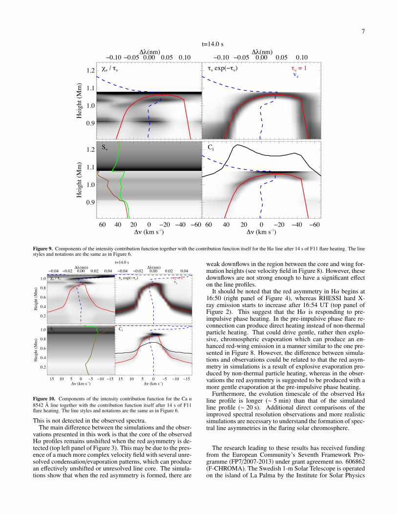
Figure 9 shows similar diagrams 14 s into the F11 flare run.Now the Hα line core is formed deeper into the atmosphere,indicating that the chromosphere is compressed by the tran-sition region which moves downward from 1.18 Mm to 1.08Mm over about 10 s (see Figures 8, 9). At the core forma-

Hα−1.4 Å 16:55:24 30% levelHXR 25−50 keV 16:54:30+90s50,60,70,80,90%

0 10 20 30 40 50arcsec

0

10

20

30

40

50

arcs

ec

Figure 6. Hα - 1.4 Å image at the flare peak (16:55:24 UT), with blue con-tours showing the 30% level of the image maximum, overlaid with a RHESSI25-50 keV reconstructed image, shown as red contours at 50, 60, 70, 80, 90%of the maximum.

tion height (at around 1.08 Mm) the atmosphere has devel-oped a moderately strong downflow (condensation) of about−18 km s−1 (downward velocities are negative) with a nega-tive velocity gradient. This shifts the central reversal (max-imum opacity) to the red side (Figure 9). The higher lyingplasma of the line core absorbs red photons, increasing theopacity in the red wing. Therefore, the red wing photons pro-duced between 0.9-1.05 Mm can no longer escape as readilyas at t=3 s because the τ = 1 curve has shifted to the red due tothe downflowing material above. As a result, the τ = 1 curveis formed higher in the atmosphere at the red wing and χν/τνis larger at the blue side of the core. This makes the contribu-tion function, and hence the emission, larger in the blue wingand the blue asymmetry is established (bottom right panel ofFigure 9).

Figure 10 shows a similar diagram for the Ca ii 8542 Å line14 s into the F11 flare. This line is much narrower and formeddeeper into the atmosphere (below 1 Mm) than Hα. The ve-locity field along this height is very weak (∼ ±1 − 2 km s−1)during the flare, and the line source function has a maxi-mum at the height of core formation (∼ 0.9 Mm) (bottom leftpanel), so the higher emission originates from the line core.An upflow velocity field below ∼ 0.8 Mm produces a slightlyextended blue wing and creates a blue asymmetry. However,a weak downflow at the height of core formation (∼ 0.9 Mm)shifts the line center to the red.

6. DISCUSSION AND CONCLUSION

The temporal evolution of the Hα line profile of the flarekernel revealed excess emission in the red wing with unshiftedline core before flare maximum, and excess emission in theblue wing with a red shifted line core after flare maximum.Numerical simulations show that in an atmosphere withoutvelocity fields, the centrally reversed Hα profile is symmetricwith respect to the line core (Canfield & Gayley 1984; Fanget al. 1993; Cheng et al. 2006). However, the dynamic modelstake into account the mass motions associated with the pro-

6

t=2 s

6562 6563 6564Wavelength (Å)

4

6

8

10

12

Inte

nsity

×10

6

t=6 s

6562 6563 6564Wavelength (Å)

t=10 s

6562 6563 6564Wavelength (Å)

t=14 s

6562 6563 6564Wavelength (Å)

0 10 20 30 40 50 60Time (s)

0.8

1.0

1.2

1.4

1.6

I B/I R

Figure 7. The temporal evolution of the synthesised Hα profiles during an F11 flare. The vertical dotted lines indicate the line center. The right panel shows theevolution of line profile asymmetry, IB/IR, calculated with the method described in Section 3.

0.9

1.0

1.1

1.2

Hei

ght (

Mm

)

−0.10 −0.05 0.00 0.05 0.10∆λ(nm)

χν / τν

−0.10 −0.05 0.00 0.05 0.10∆λ(nm)

τν exp(−τν) τν = 1vz

t=3.0 s

60 40 20 0 −20 −40 −60∆ν (km s−1)

0.9

1.0

1.1

1.2

Hei

ght (

Mm

)

Sν

60 40 20 0 −20 −40 −60∆ν (km s−1)

CI

Figure 8. Components of the intensity contribution function for the Hα line together with the contribution function itself after 3 s of F11 flare heating. Thediagrams are plotted in inverse gray scale so that darker shades indicate higher intensities. The line profile is overplotted in the contribution function diagram(bottom right panel) as a black line. Red lines indicate the height at which τ = 1. The vertical velocity structure of the plasma is overplotted as blue dashed lines.Positive velocity correspond to plasma upflows. The source function (green line) and Planck function (brown line) at the line center are overplotted in the bottomleft panels.

cesses of evaporation and condensation of the flaring material,which generate strong asymmetric signatures.

We emphasize that the analysis presented here has shownthat the red asymmetry observed in the Hα line profile is notnecessarily associated with plasma downflows, and the blueasymmetry may not be related to plasma upflows. Thus, usingthese line asymmetries as a direct measure of Doppler veloci-ties can lead to inaccurate results.

Motivated by the close match between simulations and ob-servations, we analysed components of intensity contributionfunctions for the Hα and Ca ii 8542 Å lines (based on the ap-proach presented in Carlsson & Stein 1997; Abbett & Hawley1999) We find that in the early stages of the flare the line coreof the centrally reversed Hα profile is blueshifted due to thestrong upflows at the height of core formation (bottom rightpanel of Figure 8). The velocity decreases downward towardthe wing formation regions, producing a steep positive veloc-

ity gradient. This gradient modifies the optical depth of theatmosphere in a way that higher lying (core) atoms absorbphotons with shorter wavelengths (blue wing photons) and thered asymmetry is formed (Figure 8). In the later stages the ve-locity field becomes dominated by the downflows due to theplasma condensation with strong negative velocity gradients(Figure 9). This shifts the absorption peak (wavelength ofmaximum opacity) to the red (bottom right panel of Figure 9),so the higher lying core plasma now absorbs red photons andproduces a blue asymmetry.

The Ca ii 8542 Å line in the F11 model is in emission andformed deeper into the atmosphere than Hα. The weak veloc-ity field along its formation height produces an extended bluewing in the line profile (bottom right panel of Figure 10), inagreement with the observations. The simulated profile showsa weak downflow at the height of core formation which shiftsthe line center to the red (bottom right panel of Figure 10).

7

0.9

1.0

1.1

1.2H

eigh

t (M

m)

−0.10 −0.05 0.00 0.05 0.10∆λ(nm)

χν / τν

−0.10 −0.05 0.00 0.05 0.10∆λ(nm)

τν exp(−τν) τν = 1vz

t=14.0 s

60 40 20 0 −20 −40 −60∆ν (km s−1)

0.9

1.0

1.1

1.2

Hei

ght (

Mm

)

Sν

60 40 20 0 −20 −40 −60∆ν (km s−1)

CI

Figure 9. Components of the intensity contribution function together with the contribution function itself for the Hα line after 14 s of F11 flare heating. The linestyles and notations are the same as in Figure 6.

0.2

0.4

0.6

0.8

1.0

Hei

ght (

Mm

)

−0.04 −0.02 0.00 0.02 0.04∆λ(nm)

χν / τν

−0.04 −0.02 0.00 0.02 0.04∆λ(nm)

τν exp(−τν) τν = 1vz

t=14.0 s

15 10 5 0 −5 −10 −15∆ν (km s−1)

0.2

0.4

0.6

0.8

1.0

Hei

ght (

Mm

)

Sν

15 10 5 0 −5 −10 −15∆ν (km s−1)

CI

Figure 10. Components of the intensity contribution function for the Ca ii8542 Å line together with the contribution function itself after 14 s of F11flare heating. The line styles and notations are the same as in Figure 6.

This is not detected in the observed spectra.The main difference between the simulations and the obser-

vations presented in this work is that the core of the observedHα profiles remains unshifted when the red asymmetry is de-tected (top left panel of Figure 3). This may be due to the pres-ence of a much more complex velocity field with several unre-solved condensation/evaporation patterns, which can producean effectively unshifted or unresolved line core. The simula-tions show that when the red asymmetry is formed, there are

weak downflows in the region between the core and wing for-mation heights (see velocity field in Figure 8). However, thesedownflows are not strong enough to have a significant effecton the line profiles.

It should be noted that the red asymmetry in Hα begins at16:50 (right panel of Figure 4), whereas RHESSI hard X-ray emission starts to increase after 16:54 UT (top panel ofFigure 2). This suggest that the Hα is responding to pre-impulsive phase heating. In the pre-impulsive phase flare re-connection can produce direct heating instead of non-thermalparticle heating. That could drive gentle, rather then explo-sive, chromospheric evaporation which can produce an en-hanced red-wing emission in a manner similar to the one pre-sented in Figure 8. However, the difference between simula-tions and observations could be related to that the red asym-metry in simulations is a result of explosive evaporation pro-duced by non-thermal particle heating, whereas in the obser-vations the red asymmetry is suggested to be produced with amore gentle evaporation at the pre-impulsive phase heating.

Furthermore, the evolution timescale of the observed Hαline profile is longer (∼ 5 min) than that of the simulatedline profile (∼ 20 s). Additional direct comparisons of theimproved spectral resolution observations and more realisticsimulations are necessary to understand the formation of spec-tral line asymmetries in the flaring solar chromosphere.

The research leading to these results has received fundingfrom the European Community’s Seventh Framework Pro-gramme (FP7/2007-2013) under grant agreement no. 606862(F-CHROMA). The Swedish 1-m Solar Telescope is operatedon the island of La Palma by the Institute for Solar Physics

8

(ISP) of Stockholm University in the Spanish Observatoriodel Roque de los Muchachos of the Instituto de Astrofısica deCanarias.

REFERENCES

Abbett, W. P., & Hawley, S. L. 1999, ApJ, 521, 906Allred, J. C., Hawley, S. L., Abbett, W. P., & Carlsson, M. 2005, ApJ, 630,

573Allred, J. C., Kowalski, A., F. & Carlsson, M. 2015, ApJ, 809, 104Asai, A., Ichimoto, K., Kita, R., Kurokawa, H., & Shibata, K. 2012, PASJ,

64, 20Berlicki, A. 2007, in ASP Conf. Ser. 368, The Physics of Chromospheric

Plasmas, ed. P. Heinzel, I. Dorotovic, & R. J. Rutten (San Francisco,CA:ASP), 387

Canfield, R. C., Gunkler, T. A., & Ricchiazzi, P. J. 1984, ApJ, 282, 296Canfield, R. C., & Gayley, K. G. 1987, ApJ, 322, 999Canfield, R. C., Zarro, D. M., Metcalf, T. R., & Lemen, J. R. 1990b, ApJ,

348, 333Canfield, R. C., Penn, M. J., Wulser, J.-P., & Kiplinger, A. L. 1990a, ApJ,

363, 318Carlsson, M., & Stein, R. F. 1997, ApJ, 481, 500Cheng, J. X., Ding, M. D., & Li, J. P. 2006, ApJ, 653, 733de la Beaujardiere J.-F., Kiplinger A.L., Canfield R.C., 1992, ApJ 401, 761de la Cruz Rodrıguez, J., Lofdahl, M., Sutterlin, P., Hillberg, T., & Rouppe

van der Voort, L. 2015, A&A, 573, A40Deng, N., Tritschler, A., Jing, J., et al. 2013, ApJ, 769, 112De Pontieu, B., McIntosh, S. W., Hansteen, V. H., & Schrijver, C. J. 2009,

ApJ, 701, L1Ding, M. D., & Fang, C. 1996, SoPh, 166, 437Ding, M. D., & Fang, C. 1997, A&A, 318, L17Falchi, A., Qiu, J., & Cauzzi, G. 1997, A&A, 328, 371Fang, C., Henoux, J. C., & Gan, W. Q. 1993, A&A, 274, 917Fisher, G. H., Canfield, R. C., & McClymont, A. N. 1985, ApJ, 289, 414Graham, D. R., & Cauzzi, G. 2015, ApJ, 807, L22Gan, W. Q., Rieger, E., Fang, C., & Zhang, H. Q. 1992, A&A, 266, 573Gan W.Q., Rieger E., Fang C., 1993, ApJ 416, 886

Heinzel, P., KarlickyM., KotrcP., Svestka, Z.,1994, SolarPhys. 152, 393Huang, Z., Madjarska, M. S., Koleva, K., et al. 2014, A&A, 566, A148Hudson, H. S. 2011, SSRv, 158, 5Hurford, G. J., Schmahl, E. J., Schwartz, R. A., et al. 2002, SoPh, 210, 61Ichimoto, K., & Kurokawa, H. 1984, Sol. Phys., 93, 105Ji, G. P., Kurokawa, H., Fang, C., & Huang, Y. R. 1994, Sol. Phys., 149, 195Kerr, G. S., Simoes, P. J. A., Qiu, J., & Fletcher, L. 2015,

arXiv:1508.03813v1Li, H., You, J., Yu, X., & Du, Q. 2007, SoPh, 241, 301Lin, R. P., Dennis, B. R., Hurford, G. J., et al. 2002, SoPh, 210, 3Lofdahl, M. G., Henriques, V. M. J., & Kiselman, D. 2011, A&A, 533, A82Milligan, R. O., & Dennis, B. R. 2009, ApJ, 699, 968Meegan, C., Lichti, G., Bhat, P., et al. 2009, ApJ, 702, 791Mein, P., Mein, N., Malherbe, J.-M., et al. 1997, Sol. Phys., 172, 161Neupert, W. M. 1968, ApJL, 153, L59Rubio da Costa, F., Kleint, L., Petrosian, V., Sainz Dalda, A., & Liu, W.

2014, ApJ, 804, 56Scharmer, G. B., Dettori, P. M., Lofdahl, M. G., & Shand, M. 2003b, in

Innovative Telescopes and Instrumentation for Solar Astrophysics, ed. S.Keil, & S. Avakyan, Proc. SPIE, 4853, 370

Scharmer, G. B., Bjelksjo, K., Korhonen, T. K., Lindberg, B., & Petterson,B. 2003a, in Innovative Telescopes and Instrumentation for SolarAstrophysics, ed. S. Keil, & S. Avakyan Proc. SPIE, 4853, 341

Scharmer, G. B. 2006, A&A, 447, 1111Scharmer, G. B., Narayan, G., Hillberg, T., et al. 2008, ApJ, 689, L69Schwartz, R. A., Csillaghy, A., Tolbert, A. K., et al. 2002, SoPh, 210, 165Severny, A. B. 1968, in Mass Motions in Solar Flares and Related

Phenomena, ed. Y. Oehman (Stockholm: Almqvist & Wiksell), 71Svestka, Z., Kopecky, M., & Blaha, M. 1962, Bulletin of the Astronomical

Institutes of Czechoslovakia, 13, 37Svestka, Z. 1976, Solar Flares (Berlin: SpringerTang, F. 1983, Sol. Phys., 83, 15van Noort, M., Rouppe van der Voort, L., & Lofdahl, M. G. 2005, Sol.

Phys., 228, 191Vissers, G., & Rouppe van der Voort, L. 2012, ApJ, 750, 22Wulser, J. P., & Marti, H. 1989, ApJ, 341, 1088Yu, X.-X., & Gan, W.-Q. 2006, ChA&A, 30, 294