HAL Id: inria-00405867https://hal.inria.fr/inria-00405867

Submitted on 21 Jul 2009

HAL is a multi-disciplinary open accessarchive for the deposit and dissemination of sci-entific research documents, whether they are pub-lished or not. The documents may come fromteaching and research institutions in France orabroad, or from public or private research centers.

L’archive ouverte pluridisciplinaire HAL, estdestinée au dépôt et à la diffusion de documentsscientifiques de niveau recherche, publiés ou non,émanant des établissements d’enseignement et derecherche français ou étrangers, des laboratoirespublics ou privés.

Kumar’s, Zipf ’s and Other Laws: How to Structure aLarge-Scale Wireless Network?

Mischa Dohler, Thomas Watteyne, Fabrice Valois, Jia-Liang Lu

To cite this version:Mischa Dohler, Thomas Watteyne, Fabrice Valois, Jia-Liang Lu. Kumar’s, Zipf ’s and Other Laws:How to Structure a Large-Scale Wireless Network?. Annals of Telecommunications - annales destélécommunications, Springer, 2008, 63 (5-6), pp.239-251. <inria-00405867>

Noname manuscript No.(will be inserted by the editor)

Kumar’s, Zipf’s and Other Laws:

How to Structure a Large-Scale Wireless Network?

Mischa Dohler · Thomas Watteyne

Fabrice Valois · Jia-Liang Lu

Received: 3 September 2007 / Accepted: 5 February 2008

Abstract Networks with a very large number of nodes are known to suffer from scal-

ability problems, influencing throughput, delay and other quality of service (QoS) pa-

rameters. Mainly applicable to wireless sensor networks, this paper extends the work

of [1] and aims to give some fundamental indications on a scalable and optimum (or

near-optimum) structuring approach for large-scale wireless networks. Scalability and

optimality will be defined w.r.t. various performance criteria, an example of which is

the throughput per node in the network. Various laws known from different domains

will be invoked to quantify the performance of a given topology; most notably, we will

make use of the well-known Kumar’s law, as well as less known Zipf’s and other scaling

laws. Optimum network structures are derived and discussed for a plethora of different

scenarios, facilitating knowledgeable design guidelines for these types of networks.

Keywords scalability · large-scale networks · throughput

This work is partially funded by the French ARESA RNRT Project ANR-05-RNRT-01703.

M. DohlerCTTC, Parc Mediterrani, Av. Canal Olimpic, 08860 Castelldefels, Barcelona, SpainTel.: +34-93-645 2900Fax: +34-93-645 2901E-mail: first.lastname@cttc.es

T. WatteyneFrance Telecom R&D, Meylan Cedex, F-38243, FranceTel.: +33-4-7676 2664Fax: +33-4-7676 4450E-mail: first.lastname@orange-ftgroup.com

F. Valois & J.-L. LuARES INRIA / CITI, INSA-Lyon, F-69621, FranceTel.: +33-4-7243 6418Fax: +33-4-7243 6227E-mail: first.lastname@insa-lyon.fr

2

1 Introduction

Mobile operators offer today a variety of services to its clientele, including mobile and

fixed telephony, wired and wireless Internet, as well as integrated home and business

solutions. They own large scale wired and wireless networks, with the latter tradition-

ally being composed of cellular networks and lately also of wireless sensor networks

(WSNs). Operators’ networks are composed of several million of nodes and enjoy plan-

ning and optimization prior to roll-out. WSNs are expected to be composed of several

tens of thousands of nodes and generally do not enjoy planned roll-outs.

Through cellular systems, mobile operators have already been offering 2G, 3G

and 3.5G wireless voice and date services for some years. Whilst subscriber numbers

were low at the beginning, these have risen dramatically over the past years and hence

having triggered the need to continuously augment the capacity of the cellular network.

The invoked solution consists of introducing a hierarchical communication structure in

form of cells, where several users are connected to a base station (BS), several of these

BSs are then connected to a network controller, and the network controllers are then

meshed by means of a backbone.

Whilst this facilitated scalability, such a solution is clearly expensive; for instance,

a 3G Node B may cost several hundred thousand Euros. The question hence arises

whether the approach taken is optimum or whether another solution would have been

more appropriate. Whilst the answer depends on many factors and the limited scope of

the paper prohibits all of these to be taken into account, we aim to give some indicative

answers on the optimality of the hierarchical approach.

As for wireless sensor networks, respective companies as well as operators hope

to offer more complete services by creating and facilitating ambient environments,

which interface with incumbent and emerging services in industrial and home busi-

nesses. For this reason, these companies have strong R&D activities in the area of

WSNs − exemplified by the national ARESA research project [2].

Sensor networks have been researched and deployed for decades already; their wire-

less extension, however, has witnessed a tremendous upsurge in recent years. This is

mainly attributed to the unprecedented operating conditions of WSNs, i.e. a poten-

tially enormous amount of sensor nodes reliably operating under stringent energy con-

straints. WSNs allow for an untethered sensing of the environment. It is anticipated

that within a few years, sensors will be deployed in a variety of scenarios, ranging from

environmental monitoring to health care, from the public to the private sector, etc; a

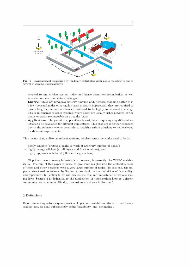
deployment example is shown in Figure 1 [3]. They will be battery-driven and deployed

in great numbers at once in an ad hoc fashion, requiring communication protocols and

embedded system components to run in an utmost energy efficient manner.

Prior to large-scale deployment, however, a gamut of problems has still to be solved

which relates to various issues, such as the design of suitable software and hardware ar-

chitectures, development of communication and organization protocols, validation and

first steps of prototyping, until the actual commercialization. In contrast to known and

well understood systems, however, a WSNs bear some fundamental design differences,

i.e. [4]:

– Number of Nodes: The number of nodes involved is very large, where current

rollout examples include a few thousands; however, roll-out expectations are in the

range of a few hundred thousand nodes communicating simultaneously. This is also

3

processing unit or gateway

node

Fig. 1 Environmental monitoring by randomly distributed WSN nodes reporting to one orseveral processing units/gateways.

atypical to any wireless system today, and hence poses new technological as well

as social and environmental challenges.

– Energy: WSNs are nowadays battery powered and, because changing batteries in

a few thousand nodes on a regular basis is clearly impractical, they are required to

have a long lifetime and are hence considered to be highly constrained in energy.

This is in contrast to other systems, where nodes are usually either powered by the

mains or easily rechargeable on a regular basis.

– Applications: The gamut of applications is vast, hence requiring very different so-

lutions to be developed for different applications. This problem is further enhanced

due to the stringent energy constraints, requiring subtle solutions to be developed

for different requirements.

This means that, unlike incumbent systems, wireless sensor networks need to be [4]:

– highly scalable (protocols ought to work at arbitrary number of nodes);

– highly energy efficient (at all layers and functionalities); and

– highly application tailored (efficient for given task).

Of prime concern among industrialists, however, is currently the WSNs’ scalabil-

ity [5]. The aim of this paper is hence to give some insights into the scalability issue

of these and other networks with a very large number of nodes. To this end, the pa-

per is structured as follows. In Section 2, we dwell on the definition of ’scalability’

and ’optimum’. In Section 3, we will discuss the role and importance of various scal-

ing laws. Section 4 is dedicated to the application of these scaling laws to different

communication structures. Finally, conclusions are drawn in Section 5.

2 Definitions

Before embarking onto the quantification of optimum scalable architectures and various

scaling laws, we shall subsequently define ’scalability’ and ’optimality’.

4

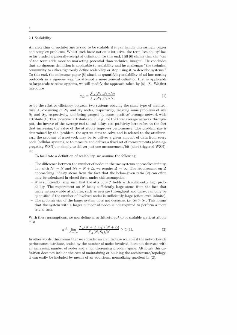
2.1 Scalability

An algorithm or architecture is said to be scalable if it can handle increasingly bigger

and complex problems. Whilst such basic notion is intuitive, the term ’scalability’ has

so far evaded a generally-accepted definition. To this end, Hill [6] claims that the ”use

of the term adds more to marketing potential than technical insight”. He concludes

that no rigorous definition is applicable to scalability and he challenges ”the technical

community to either rigorously define scalability or stop using it to describe systems.”

To this end, the milestone paper [8] aimed at quantifying scalability of ad hoc routing

protocols in a rigorous way. To attempt a more general definition that is applicable

to large-scale wireless systems, we will modify the approach taken by [6]−[8]. We first

introduce

η12 =FA(N2, S2)/N2

FA(N1, S1)/N1(1)

to be the relative efficiency between two systems obeying the same type of architec-

ture A, consisting of N1 and N2 nodes, respectively, tackling some problems of size

S1 and S2, respectively, and being gauged by some ’positive’ average network-wide

attribute F . This ’positive’ attribute could, e.g., be the total average network through-

put, the inverse of the average end-to-end delay, etc; positivity here refers to the fact

that increasing the value of the attribute improves performance. The problem size is

determined by the ’problem’ the system aims to solve and is related to the attribute;

e.g., the problem of a network may be to deliver a given amount of data from every

node (cellular system), or to measure and deliver a fixed set of measurements (data ag-

gregating WSN), or simply to deliver just one measurement/bit (alert triggered WSN),

etc.

To facilitate a definition of scalability, we assume the following:

– The difference between the number of nodes in the two systems approaches infinity,

i.e., with N1 = N and N2 = N + Δ, we require Δ → ∞. The requirement on Δ

approaching infinity stems from the fact that the below-given ratio (2) can often

only be calculated in closed form under this assumption.

– N is sufficiently large such that the attribute F holds with sufficiently high prob-

ability. The requirement on N being sufficiently large stems from the fact that

many network-wide attributes, such as average throughput and delay, can only be

quantified if the number of involved nodes is sufficiently large (often even infinite).

– The problem size of the larger system does not decrease, i.e. S2 ≥ S1. This means

that the system with a larger number of nodes is not required to perform a more

trivial task.

With these assumptions, we now define an architecture A to be scalable w.r.t. attribute

F if

η � limΔ→∞

FA(N + Δ, S2)/(N + Δ)

FA(N, S1)/N≥ O(1). (2)

In other words, this means that we consider an architecture scalable if the network-wide

performance attribute, scaled by the number of nodes involved, does not decrease with

an increasing number of nodes and a non decreasing problem space. Although this de-

finition does not include the cost of maintaining or building the architecture/topology,

it can easily be included by means of an additional normalizing quotient in (2).

5

2.2 Optimality

We are also interested in the optimality of a given architecture, i.e. network topology

with associated communication protocols. With this in mind, an optimal architecture

A w.r.t. attribute F is defined as the one which, over all possible architectures A,

maximizes η. Note that although this definition is intuitive, it is often difficult to prove

optimality over all possible architectures A. In the sequel, however, we will consider

the optimum architecture over a sub-set of all possible architectures; for instance, we

will consider only flat architectures or only hierarchical ones.

3 Scaling Laws

The first question we pose is when a network has to be considered large. To exemplify

this problem, let us presuppose systems with and without internal conflicts [4]. For

instance, two systems without conflicts are

1. our circle of true friends, comprising a small number of elements; and

2. the soldiers of an ant colony, comprising a large number of elements.

On the other hand, two systems with conflicts, frictions and competition are, for ex-

ample,

1. a few children left on their own, comprising a small number of elements; and,

2. a state without government, comprising a large number of elements.

As such, ’large’ is hence not about size [4]. It is rather about managing existing and

emerging conflicts, and hence the amount of overheads needed to facilitate (fair) com-

munication. This overhead is well reflected in the efficiency η, which needs to be max-

imized for a given attribute F . If the attribute is e.g. throughput, then a flat topology

is unlikely to be the optimum architecture, whereas a hierarchical might be a good

choice. Using different scaling laws, we will use different attributes to judge upon the

scalability of considered architectures.

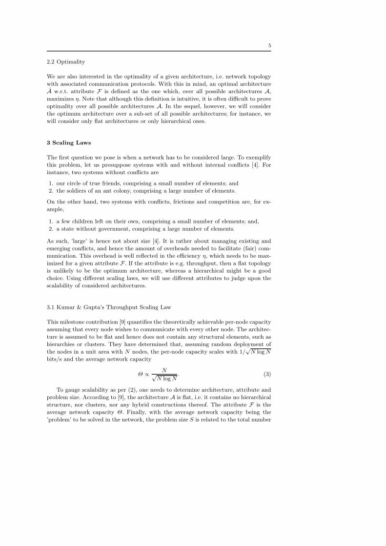
3.1 Kumar & Gupta’s Throughput Scaling Law

This milestone contribution [9] quantifies the theoretically achievable per-node capacity

assuming that every node wishes to communicate with every other node. The architec-

ture is assumed to be flat and hence does not contain any structural elements, such as

hierarchies or clusters. They have determined that, assuming random deployment of

the nodes in a unit area with N nodes, the per-node capacity scales with 1/√

N log N

bits/s and the average network capacity

Θ ∝ N√N log N

. (3)

To gauge scalability as per (2), one needs to determine architecture, attribute and

problem size. According to [9], the architecture A is flat, i.e. it contains no hierarchical

structure, nor clusters, nor any hybrid constructions thereof. The attribute F is the

average network capacity Θ. Finally, with the average network capacity being the

’problem’ to be solved in the network, the problem size S is related to the total number

6

100

101

102

103

104

10−3

10−2

10−1

100

101

102

Number of Nodes [logarithmic]

Net

wo

rk a

nd

Per

−No

de

Cap

acit

y [l

og

arit

hm

ic]

Network CapacityPer−Node Capacity

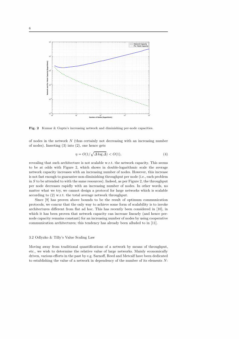
Fig. 2 Kumar & Gupta’s increasing network and diminishing per-node capacities.

of nodes in the network N (thus certainly not decreasing with an increasing number

of nodes). Inserting (3) into (2), one hence gets

η = O(1/�

Δ log Δ) < O(1), (4)

revealing that such architecture is not scalable w.r.t. the network capacity. This seems

to be at odds with Figure 2, which shows in double-logarithmic scale the average

network capacity increases with an increasing number of nodes. However, this increase

is not fast enough to guarantee non-diminishing throughput per node (i.e., each problem

in S to be attended to with the same resources). Indeed, as per Figure 2, the throughput

per node decreases rapidly with an increasing number of nodes. In other words, no

matter what we try, we cannot design a protocol for large networks which is scalable

according to (2) w.r.t. the total average network throughput.

Since [9] has proven above bounds to be the result of optimum communication

protocols, we concur that the only way to achieve some form of scalability is to invoke

architectures different from flat ad hoc. This has recently been considered in [10], in

which it has been proven that network capacity can increase linearly (and hence per-

node capacity remains constant) for an increasing number of nodes by using cooperative

communication architectures; this tendency has already been alluded to in [11].

3.2 Odlyzko & Tilly’s Value Scaling Law

Moving away from traditional quantifications of a network by means of throughput,

etc., we wish to determine the relative value of large networks. Mainly economically

driven, various efforts in the past by e.g. Sarnoff, Reed and Metcalf have been dedicated

to establishing the value of a network in dependency of the number of its elements N :

7

processing unit or gateway

wireless sensor node of zone 1

wireless sensor node of zone 2

wireless sensor node of zone 3

source wireless sensor node

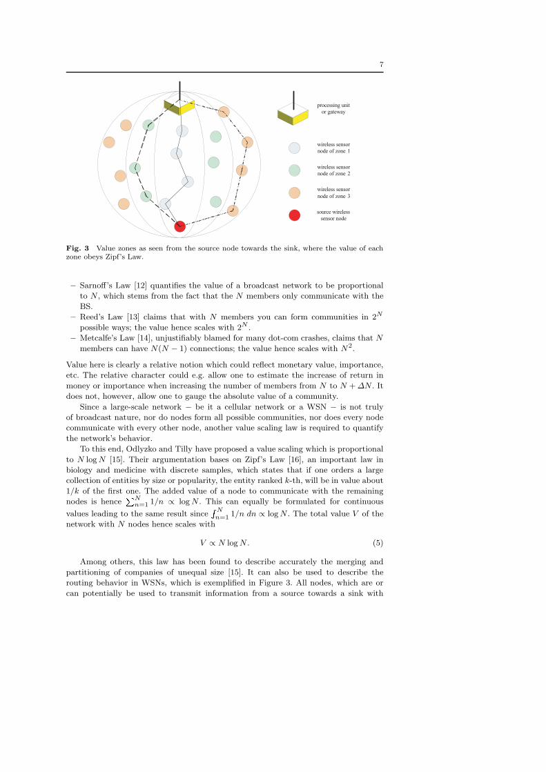
Fig. 3 Value zones as seen from the source node towards the sink, where the value of eachzone obeys Zipf’s Law.

– Sarnoff’s Law [12] quantifies the value of a broadcast network to be proportional

to N , which stems from the fact that the N members only communicate with the

BS.

– Reed’s Law [13] claims that with N members you can form communities in 2N

possible ways; the value hence scales with 2N .

– Metcalfe’s Law [14], unjustifiably blamed for many dot-com crashes, claims that N

members can have N(N − 1) connections; the value hence scales with N2.

Value here is clearly a relative notion which could reflect monetary value, importance,

etc. The relative character could e.g. allow one to estimate the increase of return in

money or importance when increasing the number of members from N to N + ΔN . It

does not, however, allow one to gauge the absolute value of a community.

Since a large-scale network − be it a cellular network or a WSN − is not truly

of broadcast nature, nor do nodes form all possible communities, nor does every node

communicate with every other node, another value scaling law is required to quantify

the network’s behavior.

To this end, Odlyzko and Tilly have proposed a value scaling which is proportional

to N log N [15]. Their argumentation bases on Zipf’s Law [16], an important law in

biology and medicine with discrete samples, which states that if one orders a large

collection of entities by size or popularity, the entity ranked k-th, will be in value about

1/k of the first one. The added value of a node to communicate with the remaining

nodes is hence�N

n=1 1/n ∝ log N . This can equally be formulated for continuous

values leading to the same result since�Nn=1 1/n dn ∝ log N . The total value V of the

network with N nodes hence scales with

V ∝ N log N. (5)

Among others, this law has been found to describe accurately the merging and

partitioning of companies of unequal size [15]. It can also be used to describe the

routing behavior in WSNs, which is exemplified in Figure 3. All nodes, which are or

can potentially be used to transmit information from a source towards a sink with

8

100

101

102

103

104

100

101

102

103

104

Number of Nodes [logarithmic]

Net

wo

rk V

alu

e [l

og

arit

hm

ic]

Odlyzko & Tilly Value Scaling LawMetcalfe Value Scaling LawSarnoff Value Scaling Law

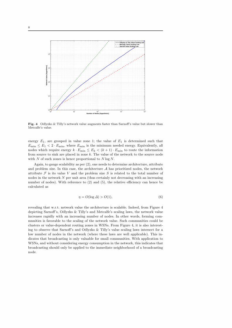
Fig. 4 Odlyzko & Tilly’s network value augments faster than Sarnoff’s value but slower thanMetcalfe’s value.

energy E1, are grouped in value zone 1; the value of E1 is determined such that

Emin ≤ E1 < 2 · Emin, where Emin is the minimum needed energy. Equivalently, all

nodes which require energy k · Emin ≤ Ek < (k + 1) · Emin to route the information

from source to sink are placed in zone k. The value of the network to the source node

with N of such zones is hence proportional to N log N .

Again, to gauge scalability as per (2), one needs to determine architecture, attribute

and problem size. In this case, the architecture A has prioritized nodes, the network

attribute F is its value V and the problem size S is related to the total number of

nodes in the network N per unit area (thus certainly not decreasing with an increasing

number of nodes). With reference to (2) and (5), the relative efficiency can hence be

calculated as

η = O(log Δ) > O(1), (6)

revealing that w.r.t. network value the architecture is scalable. Indeed, from Figure 4

depicting Sarnoff’s, Odlyzko & Tilly’s and Metcalfe’s scaling laws, the network value

increases rapidly with an increasing number of nodes. In other words, forming com-

munities is favorable to the scaling of the network value. Such communities could be

clusters or value-dependent routing zones in WSNs. From Figure 4, it is also interest-

ing to observe that Sarnoff’s and Odlyzko & Tilly’s value scaling laws intersect for a

low number of nodes in the network (where these laws are well applicable). This in-

dicates that broadcasting is only valuable for small communities. With application to

WSNs, and without considering energy consumption in the network, this indicates that

broadcasting should only be applied to the immediate neighborhood of a broadcasting

node.

9

4 Application of Scaling Laws

The above fundamental scaling laws gave us the following insights:

1. With respect to (4), the network throughput decreases with an increasing amount

of nodes due to the increasing amount of required links and hence counteracting

scalability.

2. With respect to (6), the network value increases with an increasing amount of nodes

due to the increasing amount of facilitated links and hence enabling scalability.

This apparent discrepancy is due to both laws describing two inherently different but

dependent attributes of an architecture. Indeed, the value of an architecture cannot

be guaranteed if the throughput over the required links cannot be maintained. Subse-

quently, we hence aim at exploiting and trading this dependency to find architectures

optimum under given assumptions.

Whilst not proven to be the optimum architectural solution A, the question which

naturally arises in this context is whether clusters and hierarchies will improve the

scalability of the architecture.

As described before, clusters in form of cells and hierarchies incorporating tiers of

mobile stations, tiers of node Bs, tiers of radio network controllers, etc., have been used

with success in cellular networks. Clustering has also been introduced as a means of

structuring a wireless multihop network, such as WSNs.

It is commonly assumed that using such a hierarchical architecture yields better

results than using a flat topology where all nodes have the same role. In particular,

it is assumed that clusters can reduce the volume (but not contents!) of inter-node

communication, and hence increase the network’s lifetime.

To our knowledge, solely [17] has formally studied these aspects for WSNs only with

focus on energy consumption. The authors have shown that clustered architectures

out-perform non-clustered ones in a selected number of cases. In particular, the WSN’s

energy consumption is proven to be reduced only when data aggregation is performed

by the cluster-heads.

Subsequently, we will hence examine a few selected clustering approaches and quan-

tify their scalability w.r.t. some important attributes, such as value and throughput.

4.1 Value of Clustered Network Obeying Odlyzko and Tilly’s Law

Based on Odlyzko and Tilly’s value scaling law, we introduce a normalized network

value V ′, which we define as the ratio between the value given in (5) and the number

of links per unit area needed to support such connected community. This definition

hence incorporates the required links into the value of the spanned network.

For an unclustered network, we can calculate the normalized network value V ′ as

V ′ =N log N

N log N= 1. (7)

For a clustered network, we assume C clusters and hence M = N/C nodes per

cluster. Assuming that the value of the nodes within a cluster as well as the cluster

heads obeys Zipf’s Law, the value per cluster is M log M and − with about C log C

clusters being active/valuable − the value of the clustered network is C log C ·M log M .

The average number of links needed to maintain all nodes and clusters at any time is

10

100

101

102

103

104

10−2

10−1

100

101

102

103

Number of Clusters [logarithmic]

No

rmal

ized

Net

wo

rk V

alu

e [l

og

arit

hm

ic]

N = 100 NodesN = 1000 NodesN = 10000 Nodes

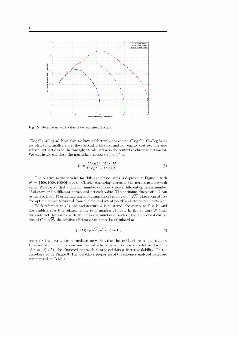
Fig. 5 Relative network value (8) when using clusters.

C log C + M log M . Note that we have deliberately not chosen C log C + CM log M as

we wish to normalize w.r.t. the spectral utilization and not energy cost per link (see

subsequent sections on the throughput calculation in the context of clustered networks).

We can hence calculate the normalized network value V ′ as

V ′ =C log C · M log M

C log C + M log M. (8)

The relative network value for different cluster sizes is depicted in Figure 5 with

N = {100, 1000, 10000} nodes. Clearly, clustering increases the normalized network

value. We observe that a different number of nodes yields a different optimum number

of clusters and a different normalized network value. The optimum cluster size C can

be derived from (8) using Lagrangian optimization yielding C =√

N , which constitutes

the optimum architecture A from the reduced set of possible clustered architectures.

With reference to (2), the architecture A is clustered, the attribute F is V ′ and

the problem size S is related to the total number of nodes in the network N (thus

certainly not decreasing with an increasing number of nodes). For an optimal cluster

size of C =√

N , the relative efficiency can hence be calculated as

η = O(log√

Δ/√

Δ) < O(1), (9)

revealing that w.r.t. the normalized network value the architecture is not scalable.

However, if compared to an unclustered scheme which exhibits a relative efficiency

of η = O(1/Δ), the clustered approach clearly exhibits a better scalability. This is

corroborated by Figure 6. The scalability properties of the schemes analyzed so far are

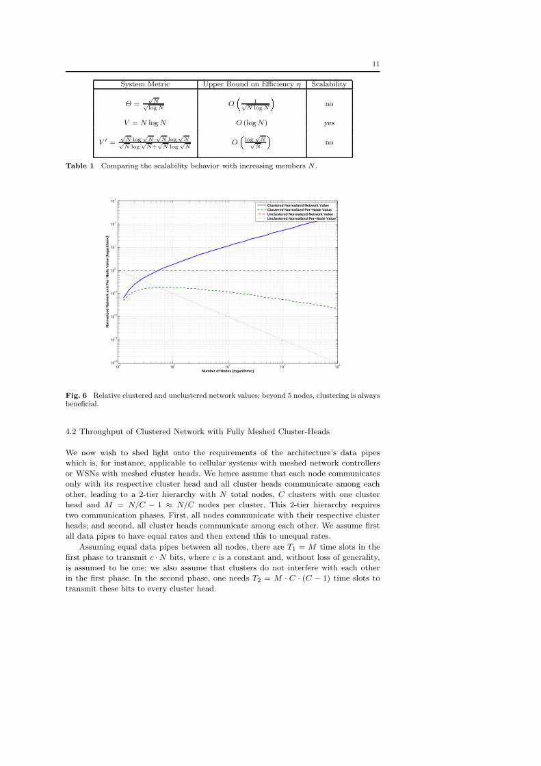
summarized in Table 1.

11

System Metric Upper Bound on Efficiency η Scalability

Θ =√

N√log N

O�

1√N log N

�no

V = N log N O (log N) yes

V ′ =√

N log√

N·√N log√

N√N log

√N+

√N log

√N

O�

log√

N√N

�no

Table 1 Comparing the scalability behavior with increasing members N .

100

101

102

103

104

10−4

10−3

10−2

10−1

100

101

102

103

Number of Nodes [logarithmic]

No

rmal

ized

Net

wo

rk a

nd

Per

−No

de

Val

ue

[lo

gar

ith

mic

]

Clustered Normalized Network ValueClustered Normalized Per−Node ValueUnclustered Normalized Network ValueUnclustered Normalized Per−Node Value

Fig. 6 Relative clustered and unclustered network values; beyond 5 nodes, clustering is alwaysbeneficial.

4.2 Throughput of Clustered Network with Fully Meshed Cluster-Heads

We now wish to shed light onto the requirements of the architecture’s data pipes

which is, for instance, applicable to cellular systems with meshed network controllers

or WSNs with meshed cluster heads. We hence assume that each node communicates

only with its respective cluster head and all cluster heads communicate among each

other, leading to a 2-tier hierarchy with N total nodes, C clusters with one cluster

head and M = N/C − 1 ≈ N/C nodes per cluster. This 2-tier hierarchy requires

two communication phases. First, all nodes communicate with their respective cluster

heads; and second, all cluster heads communicate among each other. We assume first

all data pipes to have equal rates and then extend this to unequal rates.

Assuming equal data pipes between all nodes, there are T1 = M time slots in the

first phase to transmit c ·N bits, where c is a constant and, without loss of generality,

is assumed to be one; we also assume that clusters do not interfere with each other

in the first phase. In the second phase, one needs T2 = M · C · (C − 1) time slots to

transmit these bits to every cluster head.

12

100

101

102

103

104

10−2

10−1

100

101

102

Number of Clusters [logarithmic]

No

rmal

ized

Net

wo

rk T

hro

ug

hp

ut

[lo

gar

ith

mic

]

nodes @ 1 kbps & cluster−heads @ 1 kbpsnodes @ 1 kbps & cluster−heads @ 100 kbps (Zigbee)nodes @ 1 kbps & cluster−heads @ 1 Mbps (Bluetooth)

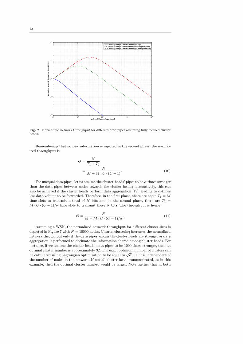
Fig. 7 Normalized network throughput for different data pipes assuming fully meshed clusterheads.

Remembering that no new information is injected in the second phase, the normal-

ized throughput is

Θ =N

T1 + T2

=N

M + M · C · (C − 1). (10)

For unequal data pipes, let us assume the cluster-heads’ pipes to be α times stronger

than the data pipes between nodes towards the cluster heads; alternatively, this can

also be achieved if the cluster heads perform data aggregation [19], leading to α-times

less data volume to be forwarded. Therefore, in the first phase, there are again T1 = M

time slots to transmit a total of N bits and, in the second phase, there are T2 =

M · C · (C − 1)/α time slots to transmit these N bits. The throughput is hence

Θ =N

M + M · C · (C − 1)/α. (11)

Assuming a WSN, the normalized network throughput for different cluster sizes is

depicted in Figure 7 with N = 10000 nodes. Clearly, clustering increases the normalized

network throughput only if the data pipes among the cluster heads are stronger or data

aggregation is performed to decimate the information shared among cluster heads. For

instance, if we assume the cluster heads’ data pipes to be 1000 times stronger, then an

optimal cluster number is approximately 32. The exact optimum number of clusters can

be calculated using Lagrangian optimization to be equal to√

α, i.e. it is independent of

the number of nodes in the network. If not all cluster heads communicated, as in this

example, then the optimal cluster number would be larger. Note further that in both

13

clustered and un-clustered cases the relative efficiency is given by η = O(1/Δ), revealing

that w.r.t. the normalized network throughput the architecture is not scalable.

Above quantification of the normalized network throughput and value of a large

network hence stipulate the use of clustered approaches. This is corroborated by real-

world roll-outs, all of which use hierarchical and/or clustered network topologies with

stronger data pipes between cluster heads. For example, the currently functioning meter

reading application of Coronis uses a hierarchical approach [20] and so does Intel’s

WSN [21].

4.3 Throughput of One-Hop Clustered Network

In this subsection, we assume that all nodes can communicate with their cluster heads

over a single hop (1-hop clusters), and that also all cluster heads can reach the sink

in a single hop. We assume again that all nodes have N bits to transmit towards

the sink node. We compare the throughput when using a clustered structure close to

LEACH [22] and direct communication.

For the clustered approach, we assume again the data pipes from cluster heads

towards sink to be α-times stronger than between sensor nodes and cluster heads.

Therefore, in the first phase, there are again T1 = M time slots to transmit N bits

and, in the second phase, there are T2 = M · C/α time slots to transmit these N bits.

The throughput is hence

Θ =N

M + M · C/α

=α · Cα + C

, (12)

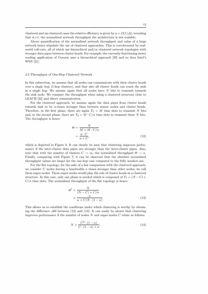
which is depicted in Figure 8. It can clearly be seen that clustering improves perfor-

mance if the inter-cluster data pipes are stronger than the intra-cluster pipes. Also,

note that with the number of clusters C → ∞, the normalized throughput Θ → α.

Finally, comparing with Figure 7, it can be observed that the absolute normalized

throughput values are larger for the one-hop case compared to the fully meshed one.

For the flat topology, for the sake of a fair comparison with the clustered approach,

we consider C nodes having a bandwidth α times stronger than other nodes; we call

them super-nodes. These super-nodes would play the role of cluster heads in a clustered

structure. In this case, only one phase is needed which is composed of T1 = (N −C) +

C/α time slots. The normalized throughput of the flat topology is hence

Θ′ =N

(N − C) + C/α

=α

α + C/N · (1 − α)(13)

This allows us to establish the conditions under which clustering is worthy by obtain-

ing the difference ΔΘ between (12) and (13). It can easily be shown that clustering

improves performance if the number of nodes N and super-nodes C relate as follows:

N >C2 · (1 − α)

C · (1 − α) + α. (14)

14

100

101

102

103

104

10−2

10−1

100

101

102

103

104

Number of Clusters [logarithmic]

No

rmal

ized

Net

wo

rk T

hro

ug

hp

ut

[lo

gar

ith

mic

]

nodes @ 1 kbps & cluster−heads @ 1 kbpsnodes @ 1 kbps & cluster−heads @ 100 kbps (Zigbee)nodes @ 1 kbps & cluster−heads @ 1 Mbps (Bluetooth)

Fig. 8 Normalized network throughput for different data pipes assuming a one-hop clusterednetwork.

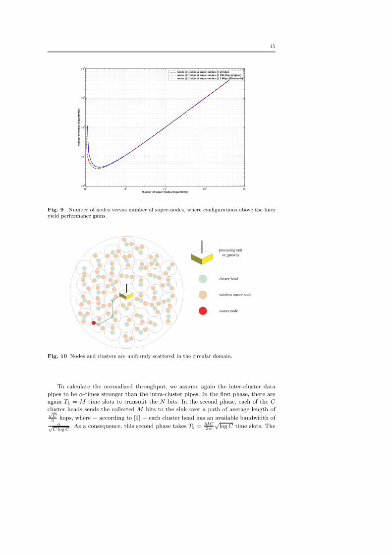
This is plotted in Figure 9, which shows that for a large number of super-nodes C

the condition of clustering being beneficial is simply C/N < 1 and for a small number

of super-nodes the number of nodes N has to be large. Note that these results are

independent of the node density as long as the assumption on the one-hop reachability

can be guaranteed.

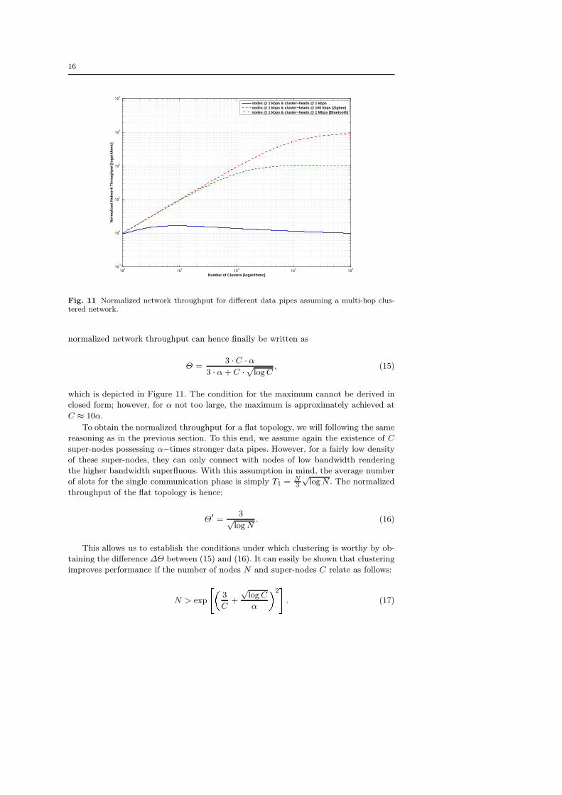
4.4 Throughput of Multi-Hop Clustered Network

In this final subsection, we assume that all nodes can communicate with their cluster

heads over a single hop (1-hop clusters), but that all cluster heads can only reach

the sink via multiple hops. To facilitate subsequent analysis, we assume the topology

model of [9], consisting of a unit area circular domain with the sink in the center; this

is illustrated in Figure 10. Such a deployment scenario is envisaged for real-world WSN

roll-outs, where the transmission power and hence also communication radius of sensor

nodes are severely limited due to the nodes’ stringent energy constraints.

To analyze this topology, we need to know the average number of hops from source

to sink. To this end, the average distance from any point of that domain to the sink

can be calculated as L =� 1√

π

0 r ·2π ·rdr = 23√

π. As per Figure 10, nodes are uniformly

scattered in the unit area domain and, to consume less energy, keep their transmission

power (thus communication range) as low as possible. Each node hence covers 1N area,

which is equivalent to a circle of diameter 1√πN

. Two neighbor nodes are thus at a

distance of r = 2√πN

and the average number of hops h = Lr between a node and the

sink can finally be calculated as h =√

N3 .

15

100

101

102

103

104

100

101

102

103

104

Number of Super−Nodes [logarithmic]

Nu

mb

er o

f N

od

es [

log

arit

hm

ic]

nodes @ 1 kbps & super−nodes @ 10 kbpsnodes @ 1 kbps & super−nodes @ 100 kbps (Zigbee)nodes @ 1 kbps & super−nodes @ 1 Mbps (Bluetooth)

Fig. 9 Number of nodes versus number of super-nodes, where configurations above the linesyield performance gains.

processing unit or gateway

cluster head

wireless sensor node

source node

Fig. 10 Nodes and clusters are uniformly scattered in the circular domain.

To calculate the normalized throughput, we assume again the inter-cluster data

pipes to be α-times stronger than the intra-cluster pipes. In the first phase, there are

again T1 = M time slots to transmit the N bits. In the second phase, each of the C

cluster heads sends the collected M bits to the sink over a path of average length of√C3 hops, where − according to [9] − each cluster head has an available bandwidth of

α√C log C

. As a consequence, this second phase takes T2 = MC3α

√log C time slots. The

16

100

101

102

103

104

10−1

100

101

102

103

104

Number of Clusters [logarithmic]

No

rmal

ized

Net

wo

rk T

hro

ug

hp

ut

[lo

gar

ith

mic

]

nodes @ 1 kbps & cluster−heads @ 1 kbpsnodes @ 1 kbps & cluster−heads @ 100 kbps (Zigbee)nodes @ 1 kbps & cluster−heads @ 1 Mbps (Bluetooth)

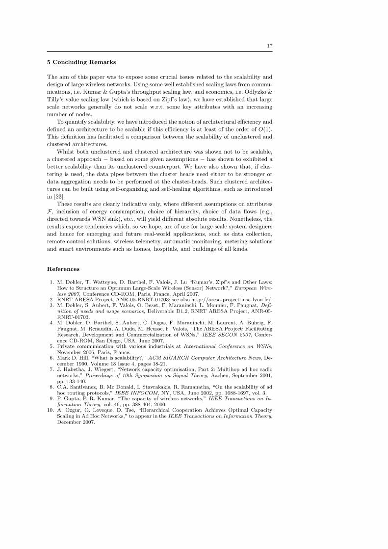
Fig. 11 Normalized network throughput for different data pipes assuming a multi-hop clus-tered network.

normalized network throughput can hence finally be written as

Θ =3 · C · α

3 · α + C · √log C, (15)

which is depicted in Figure 11. The condition for the maximum cannot be derived in

closed form; however, for α not too large, the maximum is approximately achieved at

C ≈ 10α.

To obtain the normalized throughput for a flat topology, we will following the same

reasoning as in the previous section. To this end, we assume again the existence of C

super-nodes possessing α−times stronger data pipes. However, for a fairly low density

of these super-nodes, they can only connect with nodes of low bandwidth rendering

the higher bandwidth superfluous. With this assumption in mind, the average number

of slots for the single communication phase is simply T1 = N3

√log N . The normalized

throughput of the flat topology is hence:

Θ′ =3√

log N. (16)

This allows us to establish the conditions under which clustering is worthy by ob-

taining the difference ΔΘ between (15) and (16). It can easily be shown that clustering

improves performance if the number of nodes N and super-nodes C relate as follows:

N > exp

��3

C+

√log C

α

�2�

. (17)

17

5 Concluding Remarks

The aim of this paper was to expose some crucial issues related to the scalability and

design of large wireless networks. Using some well established scaling laws from commu-

nications, i.e. Kumar & Gupta’s throughput scaling law, and economics, i.e. Odlyzko &

Tilly’s value scaling law (which is based on Zipf’s law), we have established that large

scale networks generally do not scale w.r.t. some key attributes with an increasing

number of nodes.

To quantify scalability, we have introduced the notion of architectural efficiency and

defined an architecture to be scalable if this efficiency is at least of the order of O(1).

This definition has facilitated a comparison between the scalability of unclustered and

clustered architectures.

Whilst both unclustered and clustered architecture was shown not to be scalable,

a clustered approach − based on some given assumptions − has shown to exhibited a

better scalability than its unclustered counterpart. We have also shown that, if clus-

tering is used, the data pipes between the cluster heads need either to be stronger or

data aggregation needs to be performed at the cluster-heads. Such clustered architec-

tures can be built using self-organizing and self-healing algorithms, such as introduced

in [23].

These results are clearly indicative only, where different assumptions on attributes

F , inclusion of energy consumption, choice of hierarchy, choice of data flows (e.g.,

directed towards WSN sink), etc., will yield different absolute results. Nonetheless, the

results expose tendencies which, so we hope, are of use for large-scale system designers

and hence for emerging and future real-world applications, such as data collection,

remote control solutions, wireless telemetry, automatic monitoring, metering solutions

and smart environments such as homes, hospitals, and buildings of all kinds.

References

1. M. Dohler, T. Watteyne, D. Barthel, F. Valois, J. Lu “Kumar’s, Zipf’s and Other Laws:How to Structure an Optimum Large-Scale Wireless (Sensor) Network?,” European Wire-less 2007, Conference CD-ROM, Paris, France, April 2007.

2. RNRT ARESA Project, ANR-05-RNRT-01703; see also http://aresa-project.insa-lyon.fr/.3. M. Dohler, S. Aubert, F. Valois, O. Bezet, F. Maraninchi, L. Mounier, F. Paugnat, Defi-

nition of needs and usage scenarios, Deliverable D1.2, RNRT ARESA Project, ANR-05-RNRT-01703.

4. M. Dohler, D. Barthel, S. Aubert, C. Dugas, F. Maraninchi, M. Laurent, A. Buhrig, F.Paugnat, M. Renaudin, A. Duda, M. Heusse, F. Valois, “The ARESA Project: FacilitatingResearch, Development and Commercialization of WSNs,” IEEE SECON 2007, Confer-ence CD-ROM, San Diego, USA, June 2007.

5. Private communication with various industrials at International Conference on WSNs,November 2006, Paris, France.

6. Mark D. Hill, “What is scalability?,” ACM SIGARCH Computer Architecture News, De-cember 1990, Volume 18 Issue 4, pages 18-21.

7. J. Habetha, J. Wiegert, “Network capacity optimisation, Part 2: Multihop ad hoc radionetworks,” Proceedings of 10th Symposium on Signal Theory, Aachen, September 2001,pp. 133-140.

8. C.A. Santivanez, B. Mc Donald, I. Stavrakakis, R. Ramanatha, “On the scalability of adhoc routing protocols,” IEEE INFOCOM, NY, USA, June 2002, pp. 1688-1697, vol. 3.

9. P. Gupta, P. R. Kumar, “The capacity of wireless networks,” IEEE Transactions on In-formation Theory, vol. 46, pp. 388-404, 2000.

10. A. Ozgur, O. Leveque, D. Tse, “Hierarchical Cooperation Achieves Optimal CapacityScaling in Ad Hoc Networks,” to appear in the IEEE Transactions on Information Theory,December 2007.

18

11. M. Dohler, Virtual Antenna Arrays, PhD Thesis, King’s College London, London, UK,2003.

12. K.M. Bilby, The General: David Sarnoff and the Rise of the Communications Industry,New York: Harper & Row, 1986.

13. D.P. Reed, “Weapon of math destruction: A simple formula explains why the Internet iswreaking havoc on business models,” Context Magazine, Spring 1999.

14. G. Gilder, “Metcalfe’s Law and Legacy,” Forbes ASAP, 1993.15. B. Briscoe, A. Odlyzko, B. Tilly, “Metcalfe’s Law is Wrong,” IEEE Spectrum Magazine,

July 2006.16. G.K. Zipf, “Some determinants of the circulation of information,” Amer. J. Psychology,

vol 59, 1946, pp. 401-421.17. N. Vlajic, D. Xia, “Wireless sensor networks: To cluster or not to cluster?,” International

Symposium on a World of Wireless, Mobile and Multimedia Networks (WoWMoM06),2006, pp. 258-268.

18. W. B. Heinzelman, A. P. Chandrakasan, H. Balakrishnan, “An application-specific protocolarchitecture for wireless microsensor networks, IEEE Transactions on Wireless Commu-nications, vol. 1, no. 4, pp. 660-670, 2002.

19. H. Chen, H. Mineno, T. Mizuno, “A Meta-Data-Based Data Aggregation Scheme in Clus-tering Wireless Sensor Networks,” Mobile Data Management’06, May 2006, pp. 154-154.

20. C. Dugas, “Configuring and managing a large-scale monitoring network: solving real worldchallenges for ultra-lowpowered and long-range wireless mesh networks,” Int. J. NetworkMgmt, 2005, vol 15, pp. 269-282.

21. Intel Research; see also www.intel.com/research.22. W. B. Heinzelman, A. P. Chandrakasan, and H. Balakrishnan, “An application-specific

protocol architecture for wireless microsensor networks, IEEE Transactions on WirelessCommunications, vol. 1, no. 4, pp. 660-670, 2002.

23. J.-L. Lu, F. Valois, D. Barthel, “Low-Energy Self-Organization Scheme for Wireless AdHoc Sensor Network,” IEEE WONS, January 2007, pp. 138-145.