Embed Size (px)
Citation preview
GAUSS Programmingfor Econometricians and Financial Analysts
Kuan-Pin Lin

ii
Copyright© 2001 by the publisher and author. All rights reserved. No part of this book and theaccompanied software may be reproduced, stored in a retrieval system, or transmitted by anymeans, electronic, mechanical, photocopying, recording, or otherwise, without writtenpermission of the publisher.
Limit of Liability and Disclaimer of Warranty
Although every caution has been taken in preparation this book and the accompanied software,the publisher and author make no representation or warranties with respect to the accuracy orcompleteness of the contents, and specifically disclaim any implied warranties ofmerchantability or fitness for any particular purpose, and shall in no event be liable for any lossof profit or any damages arising out of the use of this book and the accompanied software.
Trademarks
GAUSS is a trademark of Aptech Systems, Inc. GPE2 is a product name of Applied DataAssociates. All other brand names and product names used in this book are trademarks,registered trademarks, or trade names of their respective holders.

iii
PrefaceComputational Econometrics is an emerging filed of applied economics which focuses on thecomputational aspects of econometric methodology. To explore an effective and efficientapproach for econometric computation, GAUSS Programming for Econometricians andFinancial Analysts (GPE) was originally developed as the outcome of a faculty-student jointproject. The author developed the econometric program and used it in the classroom. Thestudents learned the subject materials and wrote about the experiences in using the program andGAUSS.
We know that one of the obstacles in learning econometrics is the need to do computerprogramming. Who really wants to learn a new programming language while at the same timestruggling with new econometric concepts? This is probably the reason that “easy-to-use”packages such as RATS, SHAZAM, EVIEWS, and TSP are often used in teaching andresearch. However, these canned packages are inflexible and do not allow the user sufficientfreedom in advanced modeling. GPE is an econometrics package running in GAUSSprogramming environment. You write simple codes in GAUSS to interact with GPEeconometric procedures. In the process of learning GPE and econometrics, you learn GAUSSprogramming at your own pace and for your future development.
Still, it takes some time to become familiar with GPE, not to mention the GAUSS language.The purpose of this GPE project is to provide hands-on lessons with illustrations on using thepackage and GAUSS. GPE was first developed in 1991 and has since undergone severalupdates and revisions. The first version of the project, code named LSQ, with limited functionsof least squares estimation and prediction, started in the early summer of 1995. This book/diskrepresents the major revisions of the work in progress, including linear and nonlinearregression models, simultaneous linear equation systems, and time series analysis.
Here, in your hands is the product of GPE. The best way to learn it is to read the book, type ineach lesson and run it, while exploring the sample program and output. For your convenience,all the lessons and data files are available on the distribution disk.
During several years of teaching econometrics using GPE package, many students contributedto the ideas and codes in GPE. Valuable feedback and suggestions were incorporated intodeveloping this book. In particular, the first LSQ version was a joint project with LaniPennington, who gave this project its shape. Special thanks are due to Geri Manzano, JenniferShowcross, Diane Malowney, Trish Atkinson, and Seth Blumsack for their efforts in editingand proofreading many draft versions of the manuscript and program lessons. As ways, I amgrateful to my family for their continuing support and understanding.


Table of ContentsPREFACE................................................................................................................................. IIITABLE OF CONTENTS................................................................................................................ II INTRODUCTION...................................................................................................................... 1
Why GAUSS? ...................................................................................................................... 1What is GPE?...................................................................................................................... 2How to use GPE?................................................................................................................ 2
II GAUSS BASICS .................................................................................................................. 5Getting Started.................................................................................................................... 5An Introduction to GAUSS Language................................................................................. 7Creating and Editing a GAUSS Program......................................................................... 20
Lesson 2.1 Let’s Begin.................................................................................................................21File I/O and Data Transformation.................................................................................... 24
Lesson 2.2: File I/O......................................................................................................................27Lesson 2.3: Data Transformation .................................................................................................29
GAUSS Built-In Functions................................................................................................ 30Lesson 2.4: Data Analysis............................................................................................................37
Controlling Execution Flow.............................................................................................. 38Writing Your Own Functions ............................................................................................ 42User Library ..................................................................................................................... 47GPE Package.................................................................................................................... 48
III LINEAR REGRESSION MODELS .......................................................................................... 51Least Squares Estimation.................................................................................................. 51
Lesson 3.1: Simple Regression ....................................................................................................52Lesson 3.2: Residual Analysis .....................................................................................................55Lesson 3.3: Multiple Regression..................................................................................................57
Estimating Production Function....................................................................................... 60Lesson 3.4: Cobb-Douglas Production Function .........................................................................60Lesson 3.5: Testing for Structural Change...................................................................................65Lesson 3.6: Residual Diagnostics.................................................................................................69
IV DUMMY VARIABLES......................................................................................................... 73Seasonality ........................................................................................................................ 73
Lesson 4.1: Seasonal Dummy Variables ......................................................................................74Lesson 4.2: Dummy Variable Trap ..............................................................................................78
Structural Change............................................................................................................. 79Lesson 4.3: Testing for Structural Change: Dummy Variable Approach.....................................79
V MULTICOLLINEARITY ......................................................................................................... 85Detecting Multicollinearity ............................................................................................... 85
Lesson 5.1: Condition Number and Correlation Matrix...............................................................85Lesson 5.2: Theil’s Measure of Multicollinearity ........................................................................88Lesson 5.3: Variance Inflation Factors (VIF) ..............................................................................89
Correction for Multicollinearity ....................................................................................... 91

ii
Lesson 5.4: Ridge Regression and Principal Components ...........................................................91VI NONLINEAR OPTIMIZATION.............................................................................................. 95
Solving Mathematical Functions ...................................................................................... 95Lesson 6.1: One-Variable Scalar-Valued Function......................................................................97Lesson 6.2: Two-Variable Scalar-Valued Function ...................................................................100
Estimating Probability Distributions .............................................................................. 101Lesson 6.3: Estimating Probability Distributions.......................................................................103Lesson 6.4: Mixture of Probability Distributions.......................................................................107
Statistical Regression Models ......................................................................................... 109Lesson 6.5: Minimizing Sum-of-Squares Function....................................................................110Lesson 6.6: Maximizing Log-Likelihood Function....................................................................112
VII NONLINEAR REGRESSION MODELS................................................................................ 117Nonlinear Least Squares................................................................................................. 117
Lesson 7.1: CES Production Function .......................................................................................118Maximum Likelihood Estimation .................................................................................... 119
Lesson 7.2: Box-Cox Variable Transformation .........................................................................123Statistical Inference in Nonlinear Models....................................................................... 127
Lesson 7.3: Hypothesis Testing for Nonlinear Models ..............................................................129Lesson 7.4: Likelihood Ratio Tests of Money Demand Equation..............................................132
VIII DISCRETE AND LIMITED DEPENDENT VARIABLES ........................................................ 135Binary Choice Models..................................................................................................... 135
Lesson 8.1: Probit Model of Economic Education ....................................................................138Lesson 8.2: Logit Model of Economic Education......................................................................142
Limited Dependent Variable Models .............................................................................. 144Lesson 8.3: Tobit Analysis of Extramarital Affairs....................................................................146
IX HETEROSCEDASTICITY................................................................................................... 151Heteroscedasticity-Consistent Covariance Matrix ......................................................... 151
Lesson 9.1: Heteroscedasticity-Consistent Covariance Matrix ..................................................152Weighted Least Squares.................................................................................................. 154
Lesson 9.2: Goldfeld-Quandt Test and Correction for Heteroscedasticity.................................155Lesson 9.3: Breusch-Pagan and White Tests for Heteroscedasticity..........................................157
Nonlinear Maximum Likelihood Estimation ................................................................... 159Lesson 9.4: Multiplicative Heterscedasticity..............................................................................161
X AUTOCORRELATION......................................................................................................... 165Autocorrelation-Consistent Covariance Matrix.............................................................. 165
Lesson 10.1: Heteroscedasticity-Autocorrelation-Consistent Covariance Matrix......................166Detection of Autocorrelation .......................................................................................... 169
Lesson 10.2: Tests for Autocorrelation ......................................................................................169Correction for Autocorrelation....................................................................................... 173
Lesson 10.3: Cochrane-Orcutt Iterative Procedure ....................................................................174Lesson 10.4: Hildreth-Lu Grid Search Procedure ......................................................................177Lesson 10.5: Higher Order Autocorrelation...............................................................................178
Autoregressive and Moving Average Models: An Introduction...................................... 181Lesson 10.6: ARMA(1,1) Error Structure..................................................................................183
Nonlinear Maximum Likelihood Estimation ................................................................... 186Lesson 10.7: Nonlinear ARMA Model Estimation ....................................................................187

iii
XI DISTRIBUTED LAG MODELS............................................................................................ 193Lagged Dependent Variable Models .............................................................................. 193
Lesson 11.1: Testing for Autocorrelation with Lagged Dependent Variable .............................193Lesson 11.2: Instrumental Variable Estimation .........................................................................196
Polynomial Lag Models .................................................................................................. 200Lesson 11.3: Almon Lag Model Revisited.................................................................................201
Autoregressive Distributed Lag Models.......................................................................... 203Lesson 11.4: Almon Lag Model Once More..............................................................................204
XII GENERALIZED METHOD OF MOMENTS .......................................................................... 207GMM Estimation of Probability Distributions................................................................ 207
Lesson 12.1 Gamma Probability Distribution ............................................................................210GMM Estimation of Econometric Models....................................................................... 215
Lesson 12.2 A Nonlinear Rational Expectations Model ............................................................217Linear GMM ................................................................................................................... 222
Lesson 12.3 GMM Estimation of U. S. Consumption Function ................................................223XIII SYSTEM OF SIMULTANEOUS EQUATIONS...................................................................... 225
Linear Regression Equations System.............................................................................. 225Lesson 13.1: Klein Model I........................................................................................................228Lesson 13.2: Klein Model I Reformulated.................................................................................233
Seemingly Unrelated Regression Equations System (SUR) ............................................ 236Lesson 13.3: Berndt-Wood Model.............................................................................................236Lesson 13.4: Berndt-Wood Model Extended.............................................................................240
Nonlinear Maximum Likelihood Estimation ................................................................... 242Lesson 13.5: Klein Model I Revisited........................................................................................244
XIV UNIT ROOTS AND COINTEGRATION .............................................................................. 249Testing for Unit Roots..................................................................................................... 250
Lesson 14.1: Augmented Dickey-Fuller Test for Unit Roots .....................................................252Testing for Cointegrating Regression ............................................................................. 259
Lesson 14.2: Cointegration Test: Engle-Granger Approach ......................................................261Lesson 14.3: Cointegration Test: Johansen Approach ...............................................................267
XV TIME SERIES ANALYSIS................................................................................................. 271Autoregressive and Moving Average Models ................................................................. 272
Lesson 15.1: ARMA Analysis of Bond Yields ..........................................................................274Lesson 15.2: ARMA Analysis of U. S. Inflation........................................................................278
Autoregressive Conditional Heteroscedasticity .............................................................. 279Lesson 15.3 ARCH Model of U. S. Inflation.............................................................................283Lesson 15.4 ARCH Model of Deutschemark-British Pound Exchange Rate.............................286
XVI PANEL DATA ANALYSIS............................................................................................... 291Fixed Effects Model ........................................................................................................ 292
Lesson 16.1: One-Way Panel Data Analysis: Dummy Variable Approach................................294Random Effects Model .................................................................................................... 297
Lesson 16.2: One-Way Panel Data Analysis: Deviation Approach............................................300Lesson 16.3: Two-Way Panel Data Analysis .............................................................................303
Seemingly Unrelated Regression System ........................................................................ 305Lesson 16.4: Panel Data Analysis for Investment Demand: Deviation Approach .....................306Lesson 16.5: Panel Data Analysis for Investment Demand: SUR Method.................................308

iv
XVII LEAST SQUARES PREDICTION ..................................................................................... 313Predicting Economic Growth ......................................................................................... 313
Lesson 17.1: Ex-Post Forecasts and Forecast Error Statistics....................................................315Lesson 17.2: Ex-Ante Forecasts.................................................................................................320
EPILOGUE ............................................................................................................................ 325APPENDIX A GPE CONTROL VARIABLES............................................................................ 327
Input Control Variables .................................................................................................. 327General Purpose Input Control Variables ..................................................................................328ESTIMATE Input Control Variables .........................................................................................328FORECAST Input Control Variables ........................................................................................337
Output Control Variables ............................................................................................... 338ESTIMATE Output Control Variables ......................................................................................338FORECAST Output Control Variables......................................................................................339
APPENDIX B GPE APPLICATION MODULES ........................................................................ 341Application Module B-1: GMM.GPE ............................................................................. 341Application Module B-2: JOHANSEN.GPE ................................................................... 343Application Module B-3: PANEL1.GPE......................................................................... 344Application Module B-4: PANEL2.GPE......................................................................... 346
APPENDIX C STATISTICAL TABLES ..................................................................................... 349Table C-1. Critical Values for the Dickey-Fuller Unit Root Test Based on t-Statistic .. 349Table C-2. Critical Values for the Dickey-Fuller Unit Root Test Based on F-Statistic . 351Table C-3. Critical Values for the Dickey-Fuller Cointegration t-Statistic τρ Applied onRegression Residuals ...................................................................................................... 352Table C-4. Critical Values for Unit Root and Cointegration Tests Based on ResponseSurface Estimates............................................................................................................ 353Table C-5: Critical Values for the Johansen's Cointegration Likelihood Ratio TestStatistics .......................................................................................................................... 355
REFERENCES........................................................................................................................ 357INDEX .................................................................................................................................. 359

IIntroduction
GAUSS Programming for Econometricians and Financial Analysts (GPE) is apackage of econometric procedures written in GAUSS, and this book is about GAUSSprogramming for econometric analysis and applications using GPE. To explore thecomputational aspects of applied econometrics, we adopt the programmingenvironment of GAUSS and GPE.
As you probably know, GAUSS is a programming language designed for matrix-basedoperations and manipulations, suitable for high level statistical and econometriccomputation. Many universities and research institutions have used GAUSS in theireconometric curriculum. Unfortunately, GAUSS is not an easy language to learn andmaster, particularly for those without computer programming experience. GPE isdesigned to be a bridge between the full power of GAUSS and the intimidation oflearning a new programming language. By using GPE, getting acquainted withtechniques for econometric analysis as well as the GAUSS programming environmentis fast and easy. This book was written so that you could easily use GAUSS as a toolfor econometric applications.
You can not learn econometrics by "just" reading your textbook or by "just" writingGAUSS code or programs. You must interact with the computer and textbook byworking through the examples. That is what this book is all about--learning by doing.
Why GAUSS?GAUSS is a programming language similar to C or Pascal. GAUSS code works onmatrices as the basis of a complete programming environment. It is flexible and easilyapplies itself to any kind of matrix based computation.
GAUSS comes with about 400 intrinsic commands ranging from file input/output(I/O) and graphics to high-level matrix operations. There are many GAUSS librariesand application packages, which take advantage of these built-in commands andprocedures for implementing accurate and efficient computations.
The use of libraries and packages hides complex programming details and simplifiesthe interface with a set of extended procedures and control variables. PublicationQuality Graphics of GAUSS is itself a library, extending the main system with a set ofcontrol variables manipulated on the defined graphic procedures.

GAUSS PROGRAMMING FOR ECONOMETRICIANS AND FINANCIAL ANALYSTS
2
What is GPE?GPE is a GAUSS package for linear and nonlinear regression, useful for econometricanalysis and applications. GPE contains many econometric procedures controllable bya few groups of global variables. It covers most basic econometric computationsincluding single linear equation estimation and prediction, simultaneous linearequations system, nonlinear models, and time series analysis.
However, beyond econometric computation, GPE does not provide user interface fordata input and output nor are there any procedures for data transformation. Both ofthese operations and other related topics, which build the interaction between GPEand the GAUSS programming environment, will be discussed in the next chapter onGAUSS Basics. Using the GPE package in a GAUSS environment is first introducedin Chapter III on linear least squares estimation and is the foundation of the rest of thebook.
How to use GPE?This book/disk was developed based on the latest version of GAUSS for Windows(version 3.5). Before using the GPE package, it must be properly installed with yourGAUSS program. Install GPE according to the instruction given with the distributiondisk. Make sure that the version number of GPE matches with that of your GAUSSprogram1.
Following the completion of GPE installation, the compiled GPE program namedGPE2.GCG should reside in the GAUSS directory. GPE2.GCG is a compiled GAUSSprogram. It is an encoded binary file, which requires the correct version of GAUSS. Inaddition, a GPE sub-directory is created and stores all the lesson programs and datafiles. GPE is the working directory for all the empirical lessons. By going through thisbook lesson by lesson, program files may be overwritten and additional output filesare generated. If you want a fresh start, just re-install the GPE package.
All the GPE lesson programs are written with direct reference to the GPE sub-directory created during installation. Using the default GPE sub-directory isconvenient because all the lesson programs and data files are already there for you toexplore. Alternately, you may want to use a working diskette for the practice ofcreating each lesson. If you don’t mind typing, using a working diskette is not onlyportable but also a true hands-on experience. You need only to change the referencesof the GPE sub-directory in each lesson program to the floppy drive your workingdiskette resides on (a: is assumed). That is, in the beginning of each lesson program,
1 GPE is also available for earlier versions of GAUSS.

INTRODUCTION
3
replace gpe\ with a:\. You may also need to copy the required data files to theworking diskette. A working diskette is recommended especially if you are usingGAUSS in a laboratory environment.
It is important to recognize that this book is not a GAUSS how-to manual ordocumentation, for which you are advised to consult the de facto GAUSS for WindowsUser Guide and GAUSS Language References supplied from Aptech Systems. Also,this is not a book on econometrics, although many fundamental formulas foreconometric computation are introduced in order to use the implemented algorithmsand routines. There are many textbooks on econometrics describe the technicaldetails. Rather, this is a book on computational aspects of implementing econometricmethods. We provide step by step instruction using GPE and GAUSS, complete withexplanations and sample program codes. GAUSS program codes are given in smallchunks and in piece-meal construction. Each chunk, or lesson, offers hands-onpractice for economic data analysis and econometric applications. Most examples canbe used on different computer platforms without modification.
Conventions Used in this Book
To distinguish our explanations from your typing, as seen on your video display, allprogram code and output are in monospace font Curier. For reference purpose,each line of program code is numbered. Menu items in the Windows interface,directory path and file names, and key-stroke combinations are in bold. For visualconvenience, the following icons are used:
Extra notes and additional information are given here.
This warns of common mistakes causing programming errors.
Hints or remarks specific to GAUSS and GPE2.
2 We thank Aptech Systems for permission to use their GAUSS 3.2 “hammer on numbers”icon.


II GAUSS Basics
GAUSS is a high-level computer language suitable for mathematical and matrix-oriented problem solving. It can be used to solve any kinds of mathematical,statistical, and econometric models. Since GAUSS is a computer language, it isflexible. But it is also more difficult to learn than most of canned econometricprograms such as EVIEWS, SHAZAM, and TSP.
In this chapter we begin with the very basic of starting GAUSS for Windows. Afterlearning how to get in and out of GAUSS, we discuss much of the GAUSS language.At the end of the chapter, we introduce GPE (GAUSS Programming forEconometricians and Financial Analysts) package and briefly describe its capacity foreconometric analysis and applications.
Getting StartedStart GAUSS for Windows in one of the following many ways:
• Click the short-cut (an icon with GAUSS logo) on desktop.• From Start button at the lower left corner, select and run GAUSS.• Use Windows Explorer or File Manager to locate the GAUSS directory3 and
execute the file GAUSS.EXE.
To quit and exit GAUSS for Windows, do either one of the following:
• Click and select from the menu bar: File/Exit.• Click on the “close” button (the box with the “X”) in the upper right-hand corner
of the GAUSS main window.
3 GAUSS directory refers to the directory you have successfully installed the GAUSS programin your computer. Assuming C: is your boot drive, by default installation, the GAUSS directorymay be C:\GAUSS (for Version 3.2), C:\GAUSS35 (for Version 3.5), C:\GAUSSL (for LightVersion 3.2), or C:\GAUSSLT (for Light Version 3.5). In the following, we refer C:\GAUSS asthe GAUSS directory.

GAUSS PROGRAMMING FOR ECONOMETRICIANS AND FINANCIAL ANALYSTS
6
Windows Interface
If you are new to the GAUSS programming environment, you need to spend sometimeto familiar yourself with the GAUSS Windows interface. From the menu bar, go toHelp/Contents to learn about the interface. Understanding the working function ofeach button on the menu bar, toolbar (below the menu bar), and status bar (bottom barof the main window) is the crucial beginning of GAUSS programming. The goodreference is GAUSS for Windows User Guide.
Briefly, GAUSS for Windows runs in two modes: Command and Edit. Each mode hasits own window. The Command window (or Command mode) is for running singleline command or program file. It is more commonly referred as the interactive mode.The Edit window (or Edit mode) is for modifying or editing program and data files. Afile is created from the menu bar File/New. An existing file can be open and editedfrom the menu bar File/Open. There is only one Command window, but you can openas many as Edit windows as needed for the program, data, and output, etc. Each Editwindow bears the title as the directory path and file name indicating where thecontents came from. From the Action button on the menu bar, a program file isexecuted. Your program output can be displayed either in the Command window (ifOutput mode is set to Cmnd /IO) or in a separate Output window (if Output mode isset to Split I/O). Working with multiple program and data files, GAUSS manages tokeep track of a project development in progress. Screen displays of GAUSSCommand and Edit Windows look like the following (your screen may be slightlydifferent because different configuration setup of the Windows environment you use):

GAUSS BASICS
7
You may want to configure the programming environment to fit your taste as desired.This is done from the menu bar buttons Mode and Configure. In the GAUSSprogramming environment, you can also trace and debug a program file in the Debugwindow. This is more suited for a programmer in developing a large program, whichwe will not cover in this book.
An Introduction to GAUSS Language4
The rest of this chapter covers the basic of GAUSS language. It is written for anyonewho has no prior or only limited computer programming knowledge. Only the basicsof GAUSS programming are introduced, followed by discussions of more advancedtopics useful for econometric analysis. We aspire to promote a reasonable proficiencyin reading procedures that we will write in the GAUSS language. If you are in a hurryto use the econometric package GPE for the project in hand, you can skip the rest ofthis chapter and go directly to the next chapter on linear regression models and leastsquares estimation. However we recommend that later, at your leisure, you come backfor a thorough overview of the GAUSS language.
4 This session is written based on the introduction materials of MathWorks’ MATLAB byWilliam F. Sharpe for his finance course at Stanford (http://www.stanford.edu/~wfsharpe/mia/mat/mia_mat3.htm). We thank Professor Sharpe for his helpful comments and suggestions.Both GAUSS and MATLAB are matrix programming languages, and they are syntacticalsimilar. Translation programs between GAUSS and MATLAB are available. For example, seehttp://www.goodnet.com/~dh74673/gtoml/maingtm.htm.

GAUSS PROGRAMMING FOR ECONOMETRICIANS AND FINANCIAL ANALYSTS
8
We have seen that GAUSS commands are either written in Command mode or Editmode. Command mode executes each line of code as it is written. Simple GAUSScommands can be typed and executed (by pressing the carriage return or Enter key)line by line at the “>>” prompt in the Command window5. In the beginning, tointroduce the basic commands and statements of GAUSS, we shall stay in theCommand window and use the Command or interactive mode.
Matrices as Fundamental Objects
GAUSS is one of a few languages in which each variable is a matrix (broadlyconstructed), and the language knows what the contents are and how big it is.Moreover, the fundamental operators (e.g. addition, multiplication) are programmedto deal with matrices when required. And the GAUSS environment handles much ofthe bothersome housekeeping that makes all this possible. Since so many of theprocedures required for economic and econometric computing involve matrices,GAUSS proves to be an extremely efficient language for implementation andcomputation.
First of all, each line of GAUSS code must end with a semi-colon, ";".
Consider the following GAUSS expression:
C = A + B;
If both A and B are scalars (1 by 1 matrices), C will be a scalar equal to their sum. If Aand B are row vectors of identical length, C will be a row vector of the same length.Each element of C will be equal to the sum of the corresponding elements of A and B.Finally, if A and B are, say, 3×4 matrices, C will also be a 3×4 matrix, with eachelement equal to the sum of the corresponding elements of A and B.
In short the symbol "+" means "perform a matrix addition". But what if A and B are ofincompatible sizes? Not surprisingly, GAUSS will complain with a statement such as:
(0) : error G0036 : matrices are not conformable
So the symbol "+" means "perform a matrix addition if you can and let me know ifyou can't". Similar rules and interpretation apply to matrix operations such as "-"(subtraction) and "*" (multiplication).
5 The carriage return or Enter key in the Command window is configurable within GAUSS.The default setting is “Enter always execute”. See GAUSS User Guide or online help for moreinformation.

GAUSS BASICS
9
Assignment Statements
GAUSS uses a pattern common in many programming languages for assigning thevalue of an expression to a variable. The variable name is placed on the left of anequal sign and the expression on the right. The expression is evaluated and the resultassigned to the variable. In GAUSS, there is no need to declare a variable beforeassigning a value to it. If a variable has previously been assigned a value, a number, ora string, the new value overrides the predecessor. Thus if A and B are of size 20×30,the statement:
C = A + B;
creates a variable named C that is also 20×30 and fills it with the appropriate valuesobtained by adding the corresponding elements in A and B. If C already existed andwas, say, 20×15 it would be replaced with the new 20×30 matrix. Therefore, matrixvariables in GAUSS are not fixed in size. In GAUSS, unlike some languages, there isno need to pre-dimension or re-dimension variables. It all happens without anyexplicit action on the part of the user.
Variable Names
The GAUSS environment is case insensitive. Typing variable names in uppercase,lowercase, or a combination of both does not matter. That is, GAUSS does notdistinguish between uppercase and lowercase except inside double quotes. A variablename can have up to 32 characters, including letters, numbers and underscores. Thefirst character must be alphabetic or an underscore. Therefore the variablePersonalDisposableIncome is the same aspersonaldisposableincome. While it is tempting to use long names for easyreading, small typing errors can mess up your programs. If you do mistype a variablename, you may get lucky (e.g. the system will complain that you have asked for thevalue of an undefined variable) or you may not (e.g. you will assign the new value to anewly created variable instead of the old one desired). In programming languagesthere are always tradeoffs. You don't have to declare variables in advance in GAUSS.This avoids a great deal of effort, but it allows for the possibility that nasty anddifficult-to-detect errors may creep into your programs.
Showing Values
If at any time you wish to see the contents of a variable, just type its name. GAUSSwill do its best, although the result may extend beyond the Command or Outputwindow if the variable is a large matrix (remember that you can always resize thewindow). If the variable, says x, is not defined or given a value before, a messagesuch as:

GAUSS PROGRAMMING FOR ECONOMETRICIANS AND FINANCIAL ANALYSTS
10
Undefined symbols:x (0)
will appear.
GAUSS will not show you the result of an assignment statement unless youspecifically request for it. Thus if you type:
C = A + B;
No values will be shown although C is now assigned with values of the sum of A andB. But, if you type:
C;
or, equivalently (though verbosely):
print C;
GAUSS will show you the value of C. It may be a bit daunting if C is, say, a 20 by 30matrix. If the variable C is not of interest, and what you want to see is the result of Aplus B, simply type:
A + B;
That is, if an expression has no assignment operator (=), it will be assumed to be animplicit print statement. Note that the value shown will be represented inaccordance with the format specified. If there is no explicit format used, by defaultGAUSS will show the numeric value in 16 fields with 8 digits of precision.
Initializing Matrices
If a matrix is small enough, one can provide initial values by simply typing them in theCommand window. For example:
a = 3;b = 1 2 3;c = 4, 5, 6;d = 1 2 3, 4 5 6;
Here, a is a scalar, b is a 1×3 row vector, c a 3×1 column vector, and d is a 2×3matrix. Thus, typing
d;
produces:

GAUSS BASICS
11
1.0000000 2.0000000 3.00000004.0000000 5.0000000 6.0000000
The system for indicating matrix contents is very simple. Values separated by spacesbelong on the same row; those separated by commas are on separate rows. All valuesare enclosed in brace brackets.
The alternative to creative a matrix using constants is to use GAUSS built-incommand let. If dimensions are given, a matrix of that size is created. Thefollowing statement creates a 2×3 matrix:
let d[2,3] = 1 2 3 4 5 6;
Note that dimensions of d are enclosed in square brackets, not curly bracebrackets. If dimensions are not given, a column vector is created:
let d = 1 2 3 4 5 6;
If curly braces are used, the let is optional. That is, the following twoexpressions will create the same matrix d:
let d = 1 2 3, 4 5 6;d = 1 2 3, 4 5 6;
Making Matrices from Matrices
The general scheme for initializing matrices can be extended to combine orconcatenate matrices. For example:
a = 1 2;b = 3 4;c = a~b;print c;
gives a row vector:
1.0000000 2.0000000 3.0000000 4.0000000
While:
a = 1 2 3;b = 4 5 6;d = a|b;print d;
gives a 2×3 matrix:

GAUSS PROGRAMMING FOR ECONOMETRICIANS AND FINANCIAL ANALYSTS
12
1.0000000 2.0000000 3.00000004.0000000 5.0000000 6.0000000
Matrices can easily be pasted together in this manner, a process that is both simpleand easily understood by anyone reading a procedure. Of course, the sizes of thematrices must be compatible. If they are not, GAUSS will tell you.
Note that by putting variables in brace brackets such as:
c = a b;
or
d = a,b;
will not work. It produces a syntax error message.
Using Portions of Matrices
Frequently one wishes to reference only a portion of a matrix. GAUSS providessimple and powerful ways to do so. To reference a part of a matrix, give the matrixname followed by square brackets with expressions indicating the portion desired. Thesimplest case arises when only one element is wanted. For example, using matrix d inthe previous section:
d[1,2];
equals:
2.0000000
While:
d[2,1];
equals:
4.0000000
In every case the first bracketed expression indicates the desired row (or rows), whilethe second expression indicates the desired column (or columns). If a matrix is, in

GAUSS BASICS
13
fact, a vector, a single expression may be given to indicate the desired element, but itis often wise to give both row and column information explicitly.
The real power of GAUSS comes into play when more than a single element of amatrix is wanted. To indicate "all the rows" use a dot for the first expression. Toindicate "all the columns", use a dot for the second expression. Thus,
d[1,.];
equals:
1.0000000 2.0000000 3.0000000
That is, d[1,.] yields a matrix containing the entire first row of d. While:
d[.,2];
equals:
2.00000005.0000000
That is, d[.,2] yields a matrix containing the entire second column of d. In fact,you may use any expression in this manner as long as it includes a valid row orcolumn numbers. For example:
d[2,2:3];
equals:
5.0000000 6.0000000
And:
d[2,3:2];
equals:
6.0000000 5.0000000
Variables may also be used as subscripts. Thus:

GAUSS PROGRAMMING FOR ECONOMETRICIANS AND FINANCIAL ANALYSTS
14
z = 2,3;d[2,z];
equals:
5.0000000 6.0000000
Here is another useful example:
d[1:2, 2:3];
equals:
2.0000000 3.00000005.0000000 6.0000000
This is the same as
d[.,2:3];
Try the following:
d[.,1 3];
Recall that "." is a wildcard symbol and may be used when indexing a matrix, rows orcolumns, to mean "any and all".
Text Strings
GAUSS is wonderful with numbers. It deals with text too, but one can tell that itsheart isn't in it.
A variable in GAUSS is one of two types: numeric or string. A string is like any othervariable, except the elements in it are interpreted as ASCII numbers. Thus the number32 represents a space, and the number 65 a capital A, etc. To create a string variable,enclose a string of characters in double quotation marks. Thus:
stg = "This is a string";
The variable named stg is assigned a string of characters "This is a string". Since astring variable is in fact a row vector of numbers, it is possible to create a list ofstrings by creating a matrix in which each row or column is a separate string. As withall standard matrices, each element of a string matrix can only have up to 8 characterslong, which is exactly the 32-bit size number can hold. To print a string matrix, thevariable must be prefixed with a dollar sign "$". Thus the statement:

GAUSS BASICS
15
x = "ab", "cd";print $x;
produces:
abcd
While:
x = "ab" "cd";print $x;
produces:
ab cd
as always.
To see the importance of including the dollar sign in front of a variable, type:
print x;
and see what GAUSS gives you.
Matrix and Array Operations
The term “matrix operation” is used to refer to standard procedures such as matrixmultiplication, while the term “array operation” is reserved for element-by-elementcomputations.
Matrix Operations
Matrix transposition is as easy as adding a prime (apostrophe) to the name of thematrix. Thus:
x = 1 2 3;print x';
produces:
1.00000002.00000003.0000000

GAUSS PROGRAMMING FOR ECONOMETRICIANS AND FINANCIAL ANALYSTS
16
To add two matrices of the same size, use the plus (+) sign. To subtract one matrixfrom another of the same size, use a minus (-) sign. If a matrix needs to be "turnedaround" to conform, use its transpose. Thus, if A is 3×4 and B is 4×3, the statement:
C = A + B;
results in the message:
(0) : error G0036 : matrices are not conformable
While:
C = A + B';
will get you a new 3×4 matrix C.
In GAUSS, there are some cases in which addition or subtraction works when thematrices are of different sizes. If one is a scalar, it is added to or subtracted from allthe elements in the other. If one is a row vector and its size matches with the numberof columns in the other matrix, this row vector is swept down to add or subtract thecorresponding row elements of the matrix. Similarly, if one is a column vector and itssize matches with the number of rows in the other matrix, this column vector is sweptacross to add or subtract the corresponding column elements of the matrix. Forinstance,
x = 1 2 3;y = 1 2 3, 4 5 6, 7 8 9;x + y;
produces
2.0000000 4.0000000 6.00000005.0000000 7.0000000 9.00000008.0000000 10.000000 12.000000
While,
x’ + y;
produces
2.0000000 3.0000000 4.00000006.0000000 7.0000000 8.0000000

GAUSS BASICS
17
10.000000 11.000000 12.000000
These situations are what we call “array operation” or element-by-elementcompatibility to be discussed below. GAUSS does not make syntactical distinctionbetween matrix addition (subtraction) and array addition (subtraction).
Matrix multiplication is indicated by an asterisk (*), commonly regarded inprogramming languages as a "times sign". The usual rules of matrix multiplicationfrom linear algebra apply: the inner dimensions of the two matrices being multipliedmust be the same. If they are not, you will be told so. The one allowed exception is thecase in which one of the matrices is a scalar and one is not. In this instance, everyelement of the non-scalar matrix is multiplied by the scalar, resulting in a new matrixof the same size as the non-scalar matrix.
GAUSS provides two notations for matrix division which provide rapid solutions tosimultaneous equation or linear regression problems. They are better discussed in thecontext of such problems later.
Array Operations
To indicate an array (element-by-element) multiplication, precede a standard operatorwith a period (dot). Thus:
x = 1 2 3;y = 4 5 6;x.*y;
produces
4.0000000 10.000000 18.000000
which is the "dot product" of two row vectors x and y.
You may divide all the elements in one matrix by the corresponding elements inanother, producing a matrix of the same size, as in:
C = A ./ B;
In each case, one of the operands may be a scalar or the matrices must be element-by-element compatible. This proves handy when you wish to raise all the elements in amatrix to a power. For example:
x = 1 2 3;x.^2;

GAUSS PROGRAMMING FOR ECONOMETRICIANS AND FINANCIAL ANALYSTS
18
produces
1.0000000 4.0000000 9.0000000
GAUSS array operations include multiplication (.*), division (./) and exponentiation(.^). Since the operation of exponentiation is obvious element-by-element, thenotation (.^) is the same as (^). Array addition and subtraction are discussed earlierusing the same matrix operators (+) and (-).
Logical and Relational Operations on Matrices
GAUSS offers six relational operators:
• LT or < Less than
• LE or <= Less than or equal to
• GT or > Greater than
• GE or >= Greater than or equal to
• EQ or == Equal
• NE or /= Not equal
Note carefully the difference between the double equality and the single equality.Thus A==B should be read "A is equal to B", while A=B should be read "A is assignedthe value of B". The former is a logical relation, the latter an assignment statement.For comparisons between character data and comparisons between strings, theseoperators should be preceded by a dollar sign "$".
Whenever GAUSS encounters a relational operator, it produces a one (1) if theexpression is true and a zero (0) if the expression is false. Thus the statement:
x = 1 < 3;print x;
produces:
1.0000000
GAUSS BASICS
19
While:
x = 1 > 3;print x;
produces:
0.0000000
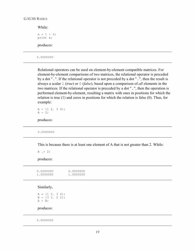
Relational operators can be used on element-by-element compatible matrices. Forelement-by-element comparisons of two matrices, the relational operator is precededby a dot ".". If the relational operator is not preceded by a dot ".", then the result isalways a scalar 1 (true) or 0 (false), based upon a comparison of all elements in thetwo matrices. If the relational operator is preceded by a dot ".", then the operation isperformed element-by-element, resulting a matrix with ones in positions for which therelation is true (1) and zeros in positions for which the relation is false (0). Thus, forexample:
A = 1 2, 3 4;A > 2;
produces:
0.0000000
This is because there is at least one element of A that is not greater than 2. While:
A .> 2;
produces:
0.0000000 0.00000001.0000000 1.0000000
Similarly,
A = 1 2, 3 4;B = 3 1, 2 2;A > B;
produces:
0.0000000

GAUSS PROGRAMMING FOR ECONOMETRICIANS AND FINANCIAL ANALYSTS
20
While:
A .> B;
produces:
0.0000000 1.00000001.0000000 1.0000000
You may also use logical operators of which we will only mention the frequently usedones in passing:
• not• and• or
If the logical operator is preceded by a dot ".", the result will be a matrix of 1's and0's based on an element-by-element logical comparison of two matrices. Each operatorworks with matrices on an element-by-element basis and conforms to the ordinaryrules of logic, treating any non-zero element as true and zero element as false.
Relational and logical operators are used frequently with if statements (describedbelow) and scalar variables, as in more mundane programming languages. But theability to use them with matrices offers major advantages in statistical andeconometric applications.
Creating and Editing a GAUSS ProgramSo far, we have seen the working of GAUSS in the Command mode. That is, at the“>>” prompt in the Command window, you enter a statement and press the carriagereturn (the Enter key) and the statement is immediately executed. GAUSS remembersall the variable names and their assigned values. Upon the execution of a statement,the available result is displayed in the Command window or in the Output windowdepending on the Output mode you use. Given the power that can be packed into oneGAUSS statement, this is no small accomplishment. However, for many purposes it isdesirable to store a set of GAUSS statements for use when needed. The simplest formof this approach is the creation and modification of a program file: a set of commandsin a file. You need to get to the Edit mode to create and edit the file. Once such a fileexists in the current directory that GAUSS knows about, you can simply load and runthe program file. The statements stored in the file will then be executed, with theresults displayed.

GAUSS BASICS
21
GAUSS for Windows provides a consistent and convenient window interface forprogram development. From the menu bar File/New (or by clicking on the bank pageicon from the toolbar), you can open a blank Edit window to create a file from scratch.If the file exists, from the menu bar File/Open (or by clicking on the open folder iconfrom the toolbar), then select the name of the file to load its contents into the Editwindow. You can also open a file in the Edit window by typing the file name in theCommand window, including the directory in which the file is stored. This Editwindow will then “pop up”, layered over the Command window. Note that the title ofthe Edit window is the name of the file you open for editing. After editing, clickingRun Current File from the Action menu button saves and runs the program file, withoutputs shown in the Command or Output window. If you are not running the programfile after editing, do not forget to save it.
A group of program and data files may be involved in a project. They can be created,loaded, and edited each in their separate Edit windows. GAUSS keeps track of twotypes of files: an active file and a main file. The active file is the file that is currentlydisplayed (in the front highlighted Edit windows). The main file is the file that isexecuted to run the current job or project. An active program file can be executed, andput in the main file list (that is, in the pull down menu on the toolbar). The main filelist contains the program files you have been running (the results of which appear inthe Command window or in the Output window). Any files on the main file list can beselected, edited, and executed repeatedly. The list of main files may be retained orcleared anytime as you wish.
Many Edit/Run cycles are involved in the writing and testing of a GAUSS program.The convention adopted in this book is that all example lessons (with only a fewexceptions such as the first one below) will be set up to have two files. The first(program) file contains the GAUSS code, and the second (output) file will contain alloutput from running the program in the first file. You will see not only the results inthe Command or Output window, but also the output is stored in a file you specified.The benefit of using Edit mode is the ability to have a record of each line of code.This is especially helpful when troubleshooting a long or complicated program.
Lesson 2.1 Let’s Begin
To get into the Edit mode, from the menu bar, select File/Open. Find and select thefile named lesson2.1 in the GPE sub-directory.
Alternatively, a file can be open from the Command window by typing the file nameat the “>>” prompt:
edit gpe\lesson2.1;
Press Enter key to load gpe\lesson2.1 into the Edit window.

GAUSS PROGRAMMING FOR ECONOMETRICIANS AND FINANCIAL ANALYSTS
22
You are now ready for program editing. The full path of file namec:\gauss\gpe\lesson2.1 (or something like that depending on your GAUSSinstallation) shows up as the title of the Edit window. lesson2.1 is just the name of theprogram file for the following exercise. GAUSS will create a file named lesson2.1 inthe c:\gauss\gpe directory if it does not already exist. If a file named lesson2.1 doesexist, GAUSS will simply bring the file to the Edit window. When working on yourown project, you should use the name of your file.
The purpose of this lesson is to demonstrate some basic matrix and array operations inthe GAUSS language we have learned so far and to familiarize you with the Edit/Rundual mode operation of GAUSS. If you are typing the following lesson for practice,do not type the line number in front of each line of code. The number system is forreference and discussion only.
1
23456789
/*** Lesson 2.1: Let’s Begin*/A = 1 2 3,
0 1 4,0 0 1;
C = 2,7,1;print"Matrix A" A;print;print "Matrix C" c;print "A*C" a*c;print "A.*C" a.*c;print "A.*C’" a.*c’;end;
From the menu bar, click on the Action button and select Run Current File. This willsave and run the program. The name of the program file lesson2.1 appears in the mainfile list located on the toolbar as a pull-down menu item. As for now, lesson2.1 is theactive file. You can run, edit, compile, and debug the main file all by clicking on thefour buttons next to the main file list.
Each line of code must end with a semi-colon, “;”. In line 1, we have typed in thenumbers in matrix form to be easier to read. Spaces separate columns while commasseparate rows. Carriage return is not seen by GAUSS. That is,
A = 1 2 3, 0 1 4, 0 0 1;
is read by GAUSS in the same way as
A = 1 2 3,0 1 4,0 0 1;

GAUSS BASICS
23
The GAUSS command, print, is used to print output to the screen. You may havewondered about the extra print statement in line 4. This creates an empty linebetween matrix A and matrix C, making the output easier to read. The rest of lesson2.1demonstrates the difference between matrix multiplication (*) and element-by-elementarray multiplication (.*) with matrices. In addition, the use of matrix transposenotation (’) is demonstrated.
After running lesson2.1, the following output should be displayed:
Matrix A1.00000000 2.0000000 3.00000000.00000000 1.0000000 4.00000000.00000000 0.0000000 1.0000000
Matrix C2.00000007.00000001.0000000
A*C19.00000011.0000001.0000000
A.*C2.0000000 4.0000000 6.00000000.00000000 7.0000000 28.0000000.00000000 0.00000000 1.0000000
A.*C’2.0000000 14.0000000 3.00000000.00000000 7.0000000 4.00000000.00000000 0.00000000 1.0000000
Notice that matrix multiplication requires that the number of columns in the firstmatrix equal the number of rows in the second matrix. Element-by-element arraymultiplication requires that both matrices have the same number of rows or columns.It “sweeps across” each row, multiplying every element of matrix A by thecorresponding element in matrix C (line 7). Element-by-element array multiplication is“swept down” each column if C is transposed first (C’) into a horizontal row vector asshown in line 8.
Programming Tips
Just a few comments on programming in general. Professional programmers judgetheir work by two criteria: does it do what it is supposed to? Is it efficient? We wouldlike to add a third criterion. Will you be able to understand what your program issupposed to be doing six months from now? Adding a blank line between sections inyour program will not effect how it runs, but it will make reading your program easier.Describing the function of each section within comment symbols will benefit you not

GAUSS PROGRAMMING FOR ECONOMETRICIANS AND FINANCIAL ANALYSTS
24
only in troubleshooting now, but also in understanding your program in the future. Todo so in GAUSS, put the comment statements in a pair of at (@) signs or in between/* and */ symbols. Notice that the * is always towards the comment text. Everythingbetween the sets of @ signs or between /* and */ symbols will be ignored by GAUSS.Comments can extend more than one line as wished. The difference between these twokinds of comments is shown in the following:
/* This kind of/* comment */
can be nested */@ This kind of comment can not be nested @
Another important programming style observed throughout this book is that we willkeep each program small. Break down your problem into smaller tasks, and write sub-programs for each task in separate blocks of a larger program or in separate programs.Avoid long lines of coding. Write clear and readable code. Use indention whereapplicable. Remember that programming is very fluid, and there are always multipleroutes to achieve any desired task.
File I/O and Data TransformationFile input and output operations (I/O) and data transformation in a GAUSSprogramming environment are important prerequisites for econometric modeling andstatistical analysis. The File I/O chapter of the GAUSS for Windows User Guidedescribes various types of file formats available in the GAUSS programmingenvironment.
Most useful programs need to communicate and interact with peripheral devices suchas file storage, console display, and printer, etc. A typical GAUSS program will readinput data from the keyboard or a file, perform computation, show results on thescreen, and send outputs to a printer or store in a file.
GAUSS can handle at least three kinds of data formats: GAUSS data sets, GAUSSmatrix files, and text (or ASCII) files. The first two data file formats are unique andefficient in GAUSS. For file transfer (import and export) between GAUSS and otherapplication software or across platforms, the text file format is preferred. Although wedo not limit the use of any particular file format, we focus here on text formatted fileinput and output. For the use of data set and matrix files, see GAUSS LanguageReferences or on-line help for more information.
Data Input
The most straightforward way to get information into GAUSS is to type it in theCommand window like what we have been doing in the first part of this chapter. Thisapproach is useful for small amount of data input. For example:

GAUSS BASICS
25
prices = 12.50 37.875 12.25;assets = "cash", "bonds", "stocks";holdings = 100 200,
300 400,500 600;
For long series of data, it is recommended that your create a text file for the data seriesusing the GAUSS Editor. That is, create the file and type the data in the Edit window.Such a file should have numeric ASCII text characters, with each element in a rowseparated from its neighbor with a space and each row on a separate line.
Now, we will introduce a text data file named longley.txt which comes with the GPEpackage. If you installed GAUSS and GPE correctly, this data file should be locatedin the GPE sub-directory of the GAUSS directory. The easiest way to bring it into theEdit window is to click on the menu bar button File/Open and select the file namelongley.txt located in the GPE directory.
The alternative is by typing in the Command window at “>>” prompt:
edit gpe\longley.txt;
and pressing Enter key.
The data matrix is arranged in seventeen rows and seven columns, and there are nomissing values. The first row contains only variable names, so it must not be includedin statistical operations. Each variable name is short, no longer than four characters inthis case. All values, except the first two columns (YEAR, and PGNP), are too largeto handle easily. Scaling these variables may make interpreting the resulting dataeasier. The bottom of the file contains the data source and description for referencepurposes. Of course, the descriptive information should not be included for statisticalanalysis.
To load the data into GAUSS, the following statement:
load data[17,7] = gpe\longley.txt;
will create a matrix named data containing the data matrix.
Alternatively, it can be re-coded as the following two lines using GAUSS commandreshape to form the desired 17×7 matrix:
load data[]=gpe\longley.txt;data=reshape(data,17,7);
Notice that the size of a matrix created with load must be equal to the size of thefile being loaded (not counting optional reference information at the bottom of the

GAUSS PROGRAMMING FOR ECONOMETRICIANS AND FINANCIAL ANALYSTS
26
file). If the matrix is larger than the actual file size, bogus data will be read. If it issmaller, part of the data series will be discarded. In either case, computations will beinaccurate.
Data Output
A simple way to output data is to display a matrix. This can be accomplished by eithergiving its name in interactive mode or using the print function as we have shown sofar.
print data;
You can use format statement to control the formats of matrices and numbersprinted out. For prettier output, the GAUSS function printfm can print a matrixusing different format for each column of the matrix.
If you want to save almost everything that appears on your screen (i.e. the output fromyour GAUSS program), issue the following command:
output file = [filename] [option];
where [filename] represents the name of a new file that will receive thesubsequent output. When using the command output file you must designate oneof three options in [option]: Reset, On, or Off. The option Reset clears all thefile contents so that each run of the program stores fresh output; On is cumulative,each output is appended to the previous one; Off creates an output file, but no data isdirected to it. An output file is not created if none of these three options is used. Whenyou are through directing output, don't forget to issue the command:
output off;
You may want to examine the output files. To create a text file containing the datafrom a matrix use output and print statements in combination. For example:
output file = gpe\output2.1 reset;print data;output off;
will save the matrix named data in the file named output2.1 in the directoryGPE.
Sending output to a printer is as easy as sending output to a file:
output file = lpt1 reset;
If you are in the Edit mode to write a program file, it is a good habit to end yourprogram with the statement:

GAUSS BASICS
27
end;
This will automatically perform output off and graciously close all the files stillopen.
Lesson 2.2: File I/O
In Lesson 2.2, we will demonstrate how to direct program output to a file and how toinput data from a text file. In addition we will slice a matrix into column vectors,which can be useful for working on individual variables. Columns (or rows) can bejoined as well. This is achieved through horizontal (or vertical) concatenation ofmatrices or vectors.
Click on the menu bar button File/Open and select the file name lesson2.2 located inthe GPE directory.
The alternative is from the Command window, at the prompt “>>”, type:
edit gpe\lesson2.2;
and press Enter.
Make sure that the highlighted Edit window, with the title c:\gauss\gpe\lesson2.2,layered over the Command window and stays in the front. To run it, click on menu barbutton Action/Run Current File.
123
4567
8910
/*** Lesson 2.2: File I/O*/output file = gpe\output2.2 reset;load data[17,7] = gpe\longley.txt;data = data[2:17,.];
PGNP = data[.,2];GNP = data[.,3]/1000;POPU = data[.,6]/1000;EM = data[.,7]/1000;
X = PGNP~GNP~POPU~EM;print X;end;
For those of you who are using a working diskette (a:\ is assumed) and want to typein the program, type these lines exactly as written. Misspellings, missing semicolons“;”, or improper spaces will all result in error messages. Be warned that each type ofbracket, , [ ], ( ), is interpreted differently. Errors commonly result from using thewrong bracket.

GAUSS PROGRAMMING FOR ECONOMETRICIANS AND FINANCIAL ANALYSTS
28
The first line of the program code tells GAUSS to direct the output of this program toa file named output2.2 located in the GPE sub-directory. If you want a printedcopy of your work, just change it to:
output file = lpt1 reset;
Let's examine the code for data loading. In line 2, a matrix named data, containing17 rows and 7 columns, is created using the GAUSS command load. A text filelocated in the GPE sub-directory named longley.txt, is then loaded into the variabledata.
Remember that the first row of data contains variable names. Chopping off the firstrow, or indexing the matrix, is one way to remove these names from statisticalanalysis. In line 3, the new data takes from the old data the second row through theseventeenth row. After line 3, the matrix named data contains 16 rows and 7columns. Now try to make some sense about what line 4 is doing. It assigns PGNP tothe second column of the modified data matrix. Notice that when a matrix is beingcreated, the brackets are to the left of the equal sign. When a matrix is indexed, thebrackets are to the right of the equal sign. In general, information is taken from theright side of an equal sign and assigned to either a matrix or variable on the left side ofthe equal sign.
The next few lines, 4 through 7, create new variables by picking the correspondingcolumns of data. For easier handling of large numbers, quantity variables are scaleddown by 1000-fold: GNP is now in billions of 1954 dollars; POPU and EM are inmillions of persons. PGNP is kept as given. Note that only the variables needed forstudy are named and identified.
We now have four variables (vectors) that have been scaled down to a workable size.Statistical operations can be done on each variable separately, or they can be joinedtogether and then operated on with one command. Line 8 concatenates all of the fourvariables horizontally with a "~" symbol, forming a new data matrix named X.
Line 9 prints the matrix X as follows:
83.000000 234.28900 107.60800 60.32300088.500000 259.42600 108.63200 61.12200088.200000 258.05400 109.77300 60.17100089.500000 284.59900 110.92900 61.18700096.200000 328.97500 112.07500 63.22100098.100000 346.99900 113.27000 63.63900099.000000 365.38500 115.09400 64.989000100.00000 363.11200 116.21900 63.761000101.20000 397.46900 117.38800 66.019000104.60000 419.18000 118.73400 67.857000108.40000 442.76900 120.44500 68.169000110.80000 444.54600 121.95000 66.513000

GAUSS BASICS
29
112.60000 482.70400 123.36600 68.655000114.20000 502.60100 125.36800 69.564000115.70000 518.17300 127.85200 69.331000116.90000 554.89400 130.08100 70.551000
If your output extends beyond your screen (in the Command or Output window), youcan resize the window for a better view. You can also try another font such as newcourier, size 10, from the Configure/Preferences button on the menu bar.
Lesson 2.3: Data Transformation
In Lesson 2.2 above, we have seen the utility of scaling data series to a moremanageable unit of measurement for analysis. For econometric applications, somevariables may be transformed for considerations of theoretical and empiricalinterpretation. Exponential, logarithmic, and reciprocal transformations are frequentlyused functional forms in econometrics. The particular chapter of GAUSS for WindowsUser Guide on Data Transformation emphasizes the use of GAUSS internal data sets.Interested readers should refer to this chapter for more details.
Lesson 2.3 below demonstrates the use of logarithmic functional transformation as away to scale the size of each data series.
For those of you who are using a working diskette (a:\ is assumed), the first twoblocks of code in lesson2.2 can be used again. Duplicating and renaming lesson2.2to lesson2.3, then editing it will save typing and time. To do that, just start withlesson2.2 in the Edit window, click on File/Save As. Since your working diskette isin a:\, make sure that in the “Select File to Save...” dialog window the “Save In:”line shows: “3 ½ Floppy (A):”. Type a:\lesson2.3 in the “File Name” line and clickon “Save”.
Here is the program lesson2.3:
123
4567
8910
/*** Lesson 2.3: Data Transformation*/output file = gpe\output2.3 reset;load data[17,7] = gpe\longley.txt;data = data[2:17,.];
PGNP = ln(data[.,2]);GNP = ln(data[.,3]/1000);POPU = ln(data[.,6]/1000);EM = ln(data[.,7]/1000);
X = PGNP~GNP~POPU~EM;print X;end;

GAUSS PROGRAMMING FOR ECONOMETRICIANS AND FINANCIAL ANALYSTS
30
Running lesson2.3, the printout of matrix X looks like this:
4.4188406 5.4565554 4.6784950 4.09971354.4830026 5.5584715 4.6879660 4.11287194.4796070 5.5531689 4.6984146 4.09719054.4942386 5.6510812 4.7088904 4.11393474.5664294 5.7959818 4.7191683 4.14663654.5859874 5.8493219 4.7297743 4.15322654.5951199 5.9009516 4.7457492 4.17421804.6051702 5.8947113 4.7554763 4.15514174.6170988 5.9851169 4.7654847 4.18994264.6501436 6.0383004 4.7768857 4.21740254.6858281 6.0930482 4.7911932 4.22198994.7077268 6.0970535 4.8036111 4.19739744.7238417 6.1794036 4.8151555 4.22909404.7379513 6.2197966 4.8312534 4.24224724.7510006 6.2503092 4.8508733 4.23889214.7613189 6.3187771 4.8681573 4.2563359
Lines 4 through 7 introduce the logarithmic transformation of each variable inaddition to simple scaling. Line 8 concatenates all these variables into a matrix namedX. This is simply the logarithmic transformation of the data matrix presented in theprevious Lesson 2.2. In GAUSS, ln computes natural log transformation of a datamatrix while log is a base 10 log transformation. We suggest the use of natural logtransformation for data scaling if needed.
GAUSS Built-In FunctionsGAUSS has a large number of built-in functions or procedures--many of which arevery powerful. Without knowing it, you have been using some of them such as let,print, load, and output. Most functions take some input arguments and returnsome outputs. Before the outputs of a function are used, they must be retrieved. To getall the outputs from a function, use a multiple assignment statement in which thevariables that are to receive the outputs are listed to the left of the equal sign,separated by commas, enclosed in brace brackets. The name of the function is on theright of the equal sign, which takes input arguments separated by commas, enclosed inround brackets. Typically, a function is called in one of the following two ways:
output1=functionName(input1);output1,output2,...=functionName(input1,input2,...);
In case the function outputs are not of interest, the command call is used to call therequested function or procedure without using any returned values. The syntax is,
call functionName(input1,input2,...);

GAUSS BASICS
31
Data Generating Functions
The following functions are particularly useful for creating a new matrix. Their usageis explained by example:
• ones Creates a 2×4 ones matrix:ones(2,4);
• zeros Creates a 4×4 zeros matrix:zeros(4,4);
• eye Creates a 3×3 identity matrix:eye(3);
• rndu Creates a 6×3 matrix of uniform random numbers:rndu(6,3);
• rndn Creates a 6×3 matrix of normal random numbers:rndn(6,3);
• seqa Creates a 10×1 vector of additive sequence of numbers starting0 with the increment 0.1 (i.e. 0, 0.1, …, 0.9):seqa(0,0.1,10);
• seqm Creates a 10×1 vector of multiplicative sequence of numbersstarting 2 with the multiplier 2 (i.e. 2, 4, …, 1032 or 210):seqm(2,2,10);
Converting or reshaping an existing matrix to a new matrix of different size, use thereshape function as in the following example:
x=seqa(1,1,5);print x;y=reshape(x,5,5);print y;
To create a sub-matrix based on some selection or deletion criteria is accomplished byselif and delif functions, respectively. For example:
x=rndn(100,4);y=selif(x, x[.,1] .> 0.5);print y;
Equivalently,
y=delif(x, x[.,1] .<= 0.5);print y;
There are other useful functions for vector or matrix conversion:
• vec Stacks columns of a matrix into a column vector.

GAUSS PROGRAMMING FOR ECONOMETRICIANS AND FINANCIAL ANALYSTS
32
• vech Stacks only the lower triangular portion of matrix into a columnvector.
• xpnd Expands a column vector into a symmetric matrix.
• submat Extracts a sub-matrix from a matrix.
• diag Retrieves the diagonal elements of a matrix.
• diagrv Replaces diagonal elements of a matrix.
Matrix Description Functions
To describe a matrix, such as a matrix x defined as
x=rndu(10,4);
the following functions can be used:
• rows Returns the number of rows of a matrix:rows(x);
• cols Returns the number of columns of a matrix :cols(x);
• maxc Returns the maximum elements of each column of a matrix:maxc(x);
• minc Returns the minimum elements of each column of a matrix:minc(x);
To find the maximum and minimum of a matrix respectively, try these:
maxc(maxc(x));minc(minc(x));
There are many other GAUSS functions like maxc and minc, which work on thecolumns of a matrix. For example:
x = 1, 2, 3;y = sumc(x) + 10;print y;
Since sumc computes the sum of each column of a matrix, this will produce:

GAUSS BASICS
33
16.000000
If a matrix is given as an argument to sumc function, the summation is appliedseparately to each column, and a column vector of results returned. Thus:
x = 1 2 3, 4 5 6;sumc(x);
The result is:
5.00000007.00000009.0000000
To compute the cumulative sum of elements in each column of a matrix, use thefunction cumsumc as follows:
cumsumc(x);
Similar to sumc and cumsumc, there are:
• prodc Computes the product of all elements in each column of amatrix.
• cumprodc Computes the cumulative product of elements in each columnof a matrix.
We further list a few descriptive statistics functions which are applied to each columnof a matrix:
• meanc Computes the mean for each column of a matrix.
• median Computes the median for each column of a matrix.
• stdc Computes the standard error for each column of a matrix.
Matrix Sorting Functions
To sort a matrix in ascending order, use one of the following sort functions:
• sortc Sorts a matrix using quick sort algorithm.
• sorthc Sorts a matrix using heap sort algorithm.

GAUSS PROGRAMMING FOR ECONOMETRICIANS AND FINANCIAL ANALYSTS
34
These functions will sort the rows of a matrix with respect to a specified column. Thatis, they will sort the elements of a column and will arrange all rows of the matrix inthe same order as the sorted column. The sort is in ascending order.
Another useful sort function, sortind, returns the sorted index of a column vector.This can be used to sort several matrices in the same way that some other referencematrix is sorted. For example:
x = 5, 2, 8;idx = sortind(x);y = x[idx];print idx~y;
produces two columns containing the ordering index of the original x and the sortedx:
2.0000000 2.00000001.0000000 5.00000003.0000000 8.0000000
Basic Matrix Computation
The following functions are related to several basic matrix computations:
• det Computes the determinant of a square matrix.
• inv Computes the inverse of a general square matrix.
• invpd Computes the inverse of a symmetric, positive definite squarematrix.
• corrx Computes a correlation matrix.
• vcx Computes a variance-covariance matrix.
• cond Computes the condition number of a matrix.
• rank Computes the rank of a matrix.

GAUSS BASICS
35
Solving Systems of Linear Equations
The problem is to find x from A*x = b, where A is a nxn matrix, b is a nx1 (or nxmin general) matrix, and x has the same size as b. If A is a non-singular matrix, then x= A-1b. Consider the following example:
a = 6 8,-2 4;
b = 2, 1;x = inv(a)*b;print x;
If the matrix A is symmetric positive definite, use the GAUSS function solpd tosolve for x. Note that the solpd function takes two arguments. The first is the matrixon the right-hand side of the matrix equation, while the second is the matrix beinginverted. For example:
a = 40 40,40 72; @ a is symmetric positive definite @
b = 2, 1;x = solpd(b,a);print x;
Therefore, if the matrix A is nxk and n is equal or greater than k, solving x from A*x= b is equivalent to solving x from (A'A)*x = (A'*b). In other words, x =invpd(A'A)*(A'b). Using the solpd function:
a = 6 8,-2 4;
b = (2, 1;x = solpd(a'b,a'a);print x;
This is exactly the GAUSS division "/" operator for finding the least squares solutionof A*x = b:
x = b/a;print x;
Another useful application of the solpd function is to find the inverse of a symmetricpositive definite matrix, which is equivalent to the invpd command:
x = solpd(eye(2),a'a); @ equivalent to invpd(a’a) @print x;
Characteristic Roots and Vectors
Given a square matrix A, finding x from the characteristic equation (A-λI)x = 0 isa two-step procedure: First, solve |A-λI| = 0 for λ (characteristic roots oreigenvalues). Then, for each λ, solve (A-λI)x = 0 for x (characteristic vectors oreigenvectors). Since we are interested in the case of real eigenvalues and eigenvectors,

GAUSS PROGRAMMING FOR ECONOMETRICIANS AND FINANCIAL ANALYSTS
36
A is assumed to be a real symmetric matrix only. Two GAUSS functions are used forthe computation of eigenvalues and eigenvectors of a real symmetric matrix:
• eigrs Computes the eigenvalues of a real symmetric matrix.
• eigrs2 Computes the eigenvalues and eigenvectors of a real symmetricmatrix.
Consider the following example:
a = 41 -23,-23 13; @ a is real and symmetric @
r = eigrs(a);r,v = eigrs2(a);print r~v;
We note that the function eigrs2 returns two values: the first is a vector ofeigenvalues, while the second is a matrix of the corresponding eigenvectors. Thereturned results are listed to the left of the equal sign, enclosed in brace brackets.Running the above block of codes, we have:
0.074175964 -0.48992502 -0.8717645753.925824 -0.87176457 0.48992502
The first column of the matrix is the vector of two eigenvalues. The last two columnsof eigenvectors correspond to each of the two eigenvalues, respectively.
An useful application of eigenvalues is to compute the condition number of a datamatrix-an indicator of multicollinearity for a least squares regression model. Let X bethe data matrix of regressors. The condition number of X is computed as follows:
xx = X'X;r = eigrs(xx);cn = sqrt(maxc(r)./minc(r));print cn;
The condition number, cn, is defined as the square root of the ratio of the largesteigenvalue to the smallest. Compared with the GAUSS built-in function cond, theidentical result is:
print cond(x);
Not listed, but of great use, are the many functions that provide data plotting in two orthree dimensions, as well as a number of more specialized functions. To whet theeconometricians' appetite, let's name a few more in the following:
• pdfn Computes the standard normal probability density function

GAUSS BASICS
37
(pdf).
• cdfn Computes the complement of cumulative distribution function(cdf) of standard normal distribution (i.e., the integral ofnormal distribution in the lower tail).
• cdftc Computes the complement of cdf of t-distribution.
• cdffc Computes the complement of cdf of F-distribution.
• cdfchic Computes the complement of cdf of chi-square distribution.
• gradp Computes the first derivative or gradient of a function.
• hessp Computes the second derivative or hessian of a function.
• intsimp Computes the integration of a function by Simpson's method.
• dstat Computes descriptive statistics of a data matrix.
• ols
Computes a typical least squares regression.
• eqsolve Solves a system of nonlinear equations.
• sqpsolve Solves the nonlinear programming problem using thesequential quadratic programming method.
The full list of functions and information on each one can be obtained via GAUSS'son-line help system.
Lesson 2.4: Data Analysis
To review what we have learned so far, in Lesson 2.4 we write a GAUSS program toload the data matrix from the file longley.txt. Examine carefully the loaded datamatrix and use only the numeric portion of each data series. Let Y be the last (7th)column of data matrix. Also, we select the first 6 variables and add a column of ones(constant vector) to form the matrix X.
First, we call the built-in function dstat to report the descriptive statistics of all dataseries including Y and X. Then the ordinary least squares estimator of Y on X iscomputed. Finally, the data matrix X is checked for its condition number.
Here is the program:

GAUSS PROGRAMMING FOR ECONOMETRICIANS AND FINANCIAL ANALYSTS
38
12345
67
89101112
/*** Lesson 2.4: Data Analysis*/output file = gpe\output2.4 reset;load x[17,7]=gpe\longley.txt;y=x[2:17,7];x=x[2:17,1:6]~ones(16,1);call dstat(0,y~x);
b=y/x; @ b=invpd(x'x)*x'y=solvpd(x'x,x'y) @print b;
xx=x'*x;r=eigrs(xx);cn=sqrt(maxc(r)./minc(r));print cn cond(x);end;
Note that in line 5, dstat is a GAUSS built-in procedure which when called printsdescriptive statistics of a data matrix into a table. The output is arranged row-wise foreach variable. In dstat, the first input argument 0 means that the data to be used is amatrix defined earlier in the program. In this case, it is the matrix y~x defined in line3 for Y and line 4 for X.
Line 6 demonstrates a simple way to obtain the least squares estimator: b = y/x.To compute the condition number of X, we first get the eigenvalues of X'X (line 9)and then take the square root of the ratio of maximum and minimum eigenvalues (line10). The result of the formal calculation of the condition number should be the sameas that from calling the GAUSS built-in function: cond. We leave the rest of runningthe program and interpreting the results to you as an exercise.
Controlling Execution FlowIt is possible to do a great deal in GAUSS by simply executing statements involvingmatrix expressions, one after the other. However, there are cases in which one simplymust substitute some non-sequential order. To facilitate this, GAUSS provides severalstandard methods for controlling program flow. In particular: For Loops, Do Loops,and If statements.
For Loops
The For Loop is easy to use. The most common use of a For Loop arises when a set ofstatements is to be repeated a fixed number of times, as in:
for i (0, 9, 1);
.......

GAUSS BASICS
39
endfor;
where i is the counter integer followed by a pair of parentheses which enclose threearguments. The first argument is the initial value of the counter, the second is its finalvalue, and the last is the increment value. The statements within the loop will beexecuted 10 times starting from the counter i at value 0 through 9, each time withincrement of 1. Note that a for loop ends with endfor statement.
There are fancier ways to use For Loops, but for our purposes, the standard onesuffices.
Do Loops
There are two kinds of Do Loops: do while and do until. The differencebetween do while loop and do until loop is that the former will continue theloop execution when the condition is true, while the latter will execute the loop whenthe condition is false (or until the condition becomes true). A Do Loop always endswith endo statement.
A do while loop contains statements to be executed as long as a stated conditionremains true, as in:
do while x <= 0.5;
.......
endo;
Similarly, A do until loop contains statements to be executed as long as a statedcondition remains false, as in:
do until x > 0.5;
.......
endo;
The statements break and continue are used within Do Loops to controlexecution flow. When break is encountered, the execution will jump to the statementfollowing the endo. This terminates the loop. When continue is encountered, theexecution will jump to the top of the loop and re-evaluate the do while or dountil expression. It reiterates the loop without executing any more of the statementsinside the loop. For the For Loops, both break and continue statements work thesame way as described for the Do Loops.
Different from the For Loop, there is no counter variable that is automaticallyincremented in a Do Loop. If one is used, it must be set to its initial value before theloop is entered and explicitly incremented or decremented inside the loop.

GAUSS PROGRAMMING FOR ECONOMETRICIANS AND FINANCIAL ANALYSTS
40
It is, of course, crucial that at some point a statement will be executed that will causethe condition in the do while (or do until) statement to be false (true). If thisis not the case, you have created an infinite loop--one that will go merrily on untilyou pull the plug.
For readability, it is sometimes useful to create variables for true and false, then usethem in a do while or do until loop. For example:
true = 1==1;false = 1==0;.....done = false;do while not done;
........
endo;
Of course, somewhere in the loop there should be a statement that will at some pointset done equal to true.
If Statements
An If statement provides a method for executing certain statements if a condition istrue and other statements (or none) if the condition is false. A complicate if sectioncan come with elseif and else statements, but it always ends with endifstatement. For example:
if x > 0.5;
.......
elseif x > 0;
.......
else;
.......
endif;
In this case, if x is greater than 0.5 the first set of statements will be executed; if not, xis checked again for a positive value. If x is greater than 0, the second set ofstatements will be executed. Otherwise, the last set of statements will be executed.
A simpler version omits the elseif section, as in:
if x > 0.5;
.......

GAUSS BASICS
41
else;
.......
endif;
In this case, if x is greater than 0.5 the first set of statements will be executed; if not,the second set will be executed. An even more simpler version omits the elsesection, as in:
If x > 0.5;
.......
endif;
Here, the statements will be executed if (and only if) x exceeds 0.5.
Nesting
All of these flow control structures allow nesting, in which one type of structure lieswithin another. For example:
j = 1;do until j > n;
for k (1,n,1);if x[j,k] > 0.5;
x[j,k] = 1.5;endif;
enfor;j=j+1;
endo;
The indentation is for the reader's benefit, but highly recommended in this and othersituations for purposes of clarity. It is wise to pair up endo (endfor, endif)statements with preceding do (for, if) statements in a last-come-first-servedmanner. It is up to the programmer to ensure that this will give the desired results.Indenting can help, but hardly guarantees success on every occasion.
While it is tempting for those with experience in traditional programming languages totake the easy way out, using Do loops for mathematical operations, this temptationshould be resisted strenuously in GAUSS. For example, instead of:
value = 0;j = 1;do while j <= n;
value = value + price[j] * quantity[j];j=j+1;
endo;
write:

GAUSS PROGRAMMING FOR ECONOMETRICIANS AND FINANCIAL ANALYSTS
42
value = price'*quantity;
The latter is more succinct, far clearer, and will run much, much faster. GAUSSperforms matrix operations at blinding speed, but is downright glacial at times whenloops are to be executed a great many times, since it must do a certain amount oftranslation of each statement every time it is encountered.
A Practical Example
Do you know the accuracy of your computer's numerical calculation? The followingexample is addressed to this important problem. Suppose e is a known small positivenumber, and the 5×4 matrix X is defined as follows:
1 1 1 1e 0 0 00 e 0 00 0 e 00 0 0 e
Verify that the eigenvalues of X'X are 4+e^2, e^2, e^2, and e^2. How small of thevalue of e your computer will allow so that X'X can be inverted? Try to make somesense out of the following segment of codes:
one=ones(1,4);e=1.0;do until e<1.0e-16;
x=one|(e.*eye(4));print "e = " e;print invpd(x'x);e=e./10;
endo;end;
Writing Your Own FunctionsThe power of GAUSS really comes into play when you add your own functions orprocedures to enhance the language. There are two kinds of user-defined functions inGAUSS. Single line functions that return one item can be defined with the fnstatement. A multi-line procedure is a group of GAUSS statements putting together toperform a given task. It is better to create a program file to hold the procedures forfuture use. Procedures are declared with the proc statement. Single line functionreturns only one argument, while multi-line procedure can return one or morearguments. Once a function or a procedure is written, debugged, and placed in thelibrary, it is for all practical purposes part of your version of GAUSS.

GAUSS BASICS
43
Single-Line Functions
A single-line function starts with a fn statement declaring the function, followed bythe name of function with its arguments enclosed in parentheses. The “guts” of thefunction is defined on the right-hand-side of the equal sign, all in one line. It is calledthe same way as GAUSS built-in functions. However, it returns only one argument.For example:
fn value(p,q) = p'*q;
This value function takes two arguments: p and q to produce the inner product ofthem. The result may be a scalar, a vector, or a matrix. Of course, this will only workif p and q vectors or matrices are compatible for matrix multiplication. A morecomplex multi-line version (or procedure) could examine the sizes of these twomatrices p and q, then use transposes, etc. as required.
It is important to note that the argument and output names used in a function arestrictly local variables that exist only within the function itself. Thus in a program, onecould write the statement to use the function:
cost = value(price,quantity);
The first matrix in the argument list of function value in this calling statement(price) would be assigned to the first argument in the function (p) while the secondmatrix in the calling statement (quantity) would be assigned to the second matrixin the function (q). This function returns the output, called cost, which is assigned tothe output argument (value). There is no need for the names to be the same in anyrespect. Moreover, the function cannot change the original arguments in any way. Itcan only return information via its output.
A powerful example of single-line function for time series conversion is the following:
fn qtoa1(x) = meanc(reshape(x,rows(x)/4,4)');
This function converts a quarterly time series into the annual series by taking theaverage of every four data points. Of course, this function will work only if the inputdata series starts from the first quarter, and it is designed to handle one series at atime. That is, the input argument x is a column vector of quarterly series, and thefunction returns a column vector of annual series. Note that if the last year does nothave the sufficient four quaterly series for conversion, it is ignored.
As another example of defining and using a single-line function statement, considerthe following scalar-valued function of one variable:
f(x) = ln(x) – x2

GAUSS PROGRAMMING FOR ECONOMETRICIANS AND FINANCIAL ANALYSTS
44
The maximal of f(x) is found at x = ½ or 0.707. This can be checked by evaluatingits first and second derivatives, respectively:
f′(x) = 1/x –2xf″(x) = -1/x2 –2
Let’s write these three single-line functions in GAUSS:
fn f(x) = ln(x) – x^2;fn f1(x) = 1/x –2*x;fn f2(x) = -1/(x^2) –2;
Now we check the maximum x = ½ for which f1(x) = 0 and f2(x) < 0:
xmax = sqrt(0.5);f(xmax);f1(xmax);f2(xmax);
Remember the built-in procedures gradp and hessp which serve the same purposeof finding the first and second derivatives, the gradient vector and hessian matrix, ofan user defined function without writing their analytical forms f1 and f2 as above.Try this:
gradp(&f,xmax);hessp(&f,xmax);
The use of gradp and hessp procedures to numerically evaluate the first andsecond derivatives of a function is useful in particular when the analytical forms ofderivatives are difficult to write. Consider the following function of two variables:
g(x) = (x12 + x2 – 11)2 + (x1 + x2
2 –7)2
With the 2×1 parameter vector x, the function is easily defined in GAUSS:
fn g(x) = (x[1]^2 + x[2] – 11)^2 + (x[1] + x[2]^2 –7)^2;
To write out the analytical formula of the first and second derivatives, using thesingle-line function may be difficult to handle the task. For this function, there are fourminima: (3, 2), (3.5844, -1.8481), (-3.7793, -3.2832), (-2.8051, 3.1313). Usinggradp and hessp to check them is easy.
At this point you may be tempted to try using a graph to find the minima of the abovefunction. GAUSS is not good at graphics. Nevertheless, there are functions availableto do publication quality graphics in GAUSS. See the GAUSS for Windows UserGuide or the on-line help menu for more details.

GAUSS BASICS
45
Procedures
A procedure in GAUSS is basically an user-defined function which can be more thanone line and as complicated as necessary to perform a given task. Any GAUSS built-in command or function may be used in a procedure, as well as any user-definedfunction or other procedure. Procedures can refer to any global variable and declarelocal variables within. The basic structure of a GAUSS procedure consists of thefollowing components:
1. proc statement
Procedure declaration
2. local statement
Local variable declaration
3. Body of procedure
…
4. retp statement
Return from procedure
5. endp statement End of procedure definition
There is always one proc statement and one endp statement in a proceduredefinition. Anything that comes between these two statements are part of theprocedure. local and retp statements are optional, and may occur more than oncein a procedure. GAUSS does not allow nested procedure definitions. That is, aprocedure can not be defined within another procedure.
Variables other than input and output arguments may be included in procedures, asneeded. There are global and local variables. A global variable is already declared andused outside the procedure. A local variable is only visible to the procedure and hasno existence outside the procedure. Indeed, a local variable in one procedure mayhave the same name as a different local variable in another function or procedure; thetwo will coexist with neither bothering the other.
A procedure can return multiple arguments of output through retp statements and byspecifying the number of returned items in the beginning of the proc statement. Asan example, the procedure version of the value function takes inputs of p and q andreturns the total (called s) and average (called m) values as follows:
proc (2) = value(p,q);local s, m;s = p'*q;m = s./sumc(q);retp(s,m);
endp;

GAUSS PROGRAMMING FOR ECONOMETRICIANS AND FINANCIAL ANALYSTS
46
In the proc statement, the syntax of an equal sign preceded with the number ofreturned arguments enclosed in parentheses (that is, "(2) = " in the above example)is not needed for a procedure with single output argument (the default case).
To use the multiple output arguments of a procedure call, simply assign them names inthe declaration line, as in:
sum,mean = value(price,quantity);
Here, variables price and quantity are assigned to the input arguments p and q,respectively. Similarly, sum and mean are assigned to the output arguments s and m.All the input and output arguments are local variables.
Note that as with inputs, the correspondence between outputs in the calling statementand the procedure itself is strictly by order. When the procedure has finished its work,its output values are assigned to the variables in the calling statement.
If a procedure does not return any items or you want to discard the returned items, justcall it as we have demonstrated in the above example lessons. For example:
call value(price,quantity);
Now let's extend from the earlier single-line version of time series conversion functionqtoa1 to a multi-line procedure so that it can handle the conversion of a moregeneral data matrix. The working of the following procedure qtoa is to take a datamatrix x which consists of quarterly data series in columns and convert it into a matrixof the yearly averages. The procedure takes advantage of the previously definedsingle-line function qtoa1 to compute the annual average series from each column ofthe quarterly data matrix, all in a do loop. Here is the procedure:
proc qtoa(x);local r,c,y,i;r = rows(x);c = cols(x);y = qtoa1(x[.,1]);i = 2;do until i > c;
y = y~qtoa1(x[.,i]);i = i+1;
endo;retp(y);
endp;
Of course, the above time series conversion function and procedure are limited to thequarterly data series. We can make them more flexible by specifying the number ofperiods of each seasonal cycle as an input argument in addition to the data matrix.
The following function tss1 and procedure tss are essentially the same as qtoa1and qtoa, respectively. The difference is that now the number of periods n for time

GAUSS BASICS
47
series conversion is specified as one of the input arguments. Depending on theseasonal cycle of the data series, you can use the same procedure for either quarterlyor monthly conversion.
fn tss1(x,n) = meanc(reshape(x,rows(x)/n,n)');
proc tss(x,n);local r,c,y,i;r = rows(x);c = cols(x);y = tss1(x[.,1],n);i = 2;do until i > c;
y = y~tss1(x[.,i],n);i = i+1;
endo;retp(y);
endp;
As an exercise, write the procedures to compute the analytical first and secondderivatives of the scalar-valued function of two variables:
g(x) = (x12 + x2 – 11)2 + (x1 + x2
2 –7)2
User LibraryThe purpose of writing functions and procedures is to keep tasks organized and self-contained. Each function or procedure will perform a few given tasks and nothingelse. To make the programmers' work easier, procedures allow programmers to buildon their previous work and on the works of others rather than starting over again andagain to perform related tasks. One way to organize the work is to collect a group offunctions and procedures into a program file and relate the file and its contents withthe GAUSS library system. Note that you must have your own copy of GAUSSinstalled on your own computer in order to access and modify the GAUSS libraryfacility. We will assume that your GAUSS comes with the User Library which you canadd your creative functions and procedures.
First, let's put the function tss1 and procedure tss together in a file namedTSS.SRC (SRC is the adopted file extension name for GAUSS source codes, althoughyou can use any other name you want). Put the program file TSS.SRC in the SRCsubdirectory of GAUSS path. Next, we will add the following lines to the library fileUSER.LCG located in the LIB directory of GAUSS path:
TSS.SRCtss1 : fntss : proc
Similar to the idea of using a dictionary, the function tss1 and procedure tssdefined in the program file TSS.SRC are now part of GAUSS library system, which

GAUSS PROGRAMMING FOR ECONOMETRICIANS AND FINANCIAL ANALYSTS
48
will be searched for name resolution every time GAUSS executes a program. You canalso add variable names as a matrices or strings in the library. Refer to the GAUSSLanguage References or on-line help system for more details on using andmaintaining the library system.
From now on, both tss1 and tss functions are an integral part of your version ofGAUSS. You have just extended the environment for GAUSS programming!
GPE PackageThe other way of extending GAUSS is to use a package, which is a set of compiledGAUSS libraries for special purposes. GAUSS Programming for Econometriciansand Financial Analysts (GPE2) is a GAUSS package of econometric procedures. TheGAUSS command use is used to load a package at the beginning of your program.For example,
use gpe2;
will load the GPE package (version 2) for econometric analysis and applications. Notethat use can appear only once at the top of a program.
GPE consists of three main procedures (estimate, forecast, and reset) alongwith global control variables that modify the econometric routines. The procedureestimate computes linear and nonlinear regressions, while forecast performsleast squares prediction. reset initializes global control variables to their defaultvalues. Global control variables are of two types: input and output. Global inputvariables control the execution behavior of the called procedure. For example, theycan modify estimate and forecast to use linear restrictions, weighted variables,instrumental variables, lagged dependent and independent variables, etc.
Output global variables are the results of calling estimate and forecast. Theycan be assigned to new variables for further analysis. Depending on the input globalvariables used which control the econometric routines, not all the output globalvariables will be available. The name of an input control variable starts with a singleunderscore (for example, _b), while an output control variable starts with a doubleunderscore (for example, __b). Refer to Appendix A for a complete list of GPEglobal control variables and their default or pre-defined values.
A template for a typical program using GPE is given below:
1
/*** Comments on program title, purposes,** and the usage of the program*/
use gpe2; @ using GPE package (version 2) @

GAUSS BASICS
49
.
.
.
@ this must be the first executable statement @
/*** Writing output to file or sending it to printer:** specify file name for output*/
/*** Loading data:** read data series from data files.*/
/*** Generating or transforming data series:** create and generate variables with** data scaling or transformation** (e.g. y and x are generated here and will be used below)*/
call reset; @ initialize global variables @
/*** Set input control variables for model estimation** (e.g. _names for variable names, see Appendix A)*/
call estimate(y,x); @ do model estimation @@ variables y, x are generated earlier @
/*** Retrieve output control variables for** model evaluation and analysis*/
/*** Set more input control variables if needed,** for model prediction** (e.g. _b for estimated parameters)*/
call forecast(y,x); @ do model prediction @
end; @ important: don’t forget this @
Using the GPE package in a GAUSS environment is the main focus of the rest of thisbook, which begins in the next chapter on linear regression models. If you are alreadyfamiliar with the linear least squares, you can jump on the nonlinear models whichbegins in Chapter VI. The topic of simultaneous equation systems is covered inChapter XIII. In addition to many classical econometric methods, modern approachessuch as generalized method of moments (Chapter XII), autoregressive conditionalheteroscedasticity (Chapter XV), and panel data analysis (Chapter XVI), areprogrammed and solved with GPE (version 2) for GAUSS.
Don't forget that we are learning GAUSS as a tool to do econometrics. Using thepackage GPE written in GAUSS is the intermediate bridge between the domain

GAUSS PROGRAMMING FOR ECONOMETRICIANS AND FINANCIAL ANALYSTS
50
knowledge (econometrics) and the programming environment (GAUSS). With thisapproach, only a limited knowledge of computer programming is required in thebeginning. After gaining experience with GPE and GAUSS in general, you should beready for your own programming adventure in advanced econometrics, by eitherextending GPE or writing new programs.

IIILinear Regression Models
GPE (GAUSS Programming for Econometricians and Financial Analysts) is aGAUSS package for linear and nonlinear regressions useful for econometric analysisand applications. The purpose of this chapter is to show you how to use GPE for basiclinear least squares estimation.
Least Squares EstimationA linear regression model can be written either in a matrix form:
Y = Xβ + ε
or, in a vector form:
Y = X1β1 + X2β2 + … + XKβK + ε
Where Y is the dependent variable, Xk is the k-th independent (explanatory) variable,and βk is the corresponding parameter (coefficient), k = 1,2,…,K. Given a sample ofN data observations, both Xk’s and Y are N-vector of sample data. Denote X = [X1 X2… XK]. Typically, we assume the last column of data matrix X, that is XK, is aconstant one-vector. For parameter estimation of a linear regression model, therandom error term ε is assumed to be identically independently distributed (iid). Forstatistical inference, an assumption of probability density will be necessary. Forexample, ε is normally identically independently distributed (nid) with zero mean andconstant variance σ2.
The ordinary least squares regression amounts to the following estimation results:
b = (X’X)-1X’Y Estimator of β.Var(b) = s2(X’X)-1 Estimated variance-covariance matrix of β.e = Y - Xb Estimated errors ε or residuals.s2 = e’e/N-K Estimated regression variance σ2. N is the number of
sample data; K the is the number of parameters.

GAUSS PROGRAMMING FOR ECONOMETRICIANS AND FINANCIAL ANALYSTS
52
Consider the simple case of regressing the dependent variable Y against oneindependent variable X in addition to a constant:
Y = α + βX + ε
where ε is the difference between known Y and estimated Y, or the residual. Theparameter α is the intercept and β is the slope of the linear regression equation.
Continuing with the text data file longley.txt we used in Chapter II, Lesson 3.1introduces the use of GPE to estimate a simple regression equation. Lesson 3.2examines a set of regression statistics obtained from the simple regression. Lesson 3.3is a multiple regression model.
Lesson 3.1: Simple Regression
This lesson estimates a simple regression relationship between employment EM inmillions of persons and RGNP or real GNP expressed in billions of 1954 dollars. Notethat the 1954 observation of PGNP is 100, which is the base year of the deflator. Alldata series are read from the text data file longley.txt.
1234
5678
9101112
/*** Lesson 3.1: Simple Regression*/use gpe2; @ using GPE package (version 2) @output file = gpe\output3.1 reset;load data[17,7] = gpe\longley.txt;data = data[2:17,.];
PGNP = data[.,2];GNP = data[.,3]/1000;EM = data[.,7]/1000;RGNP = 100*GNP./PGNP;
call reset;_names = "EM","RGNP";call estimate(EM,RGNP);end;
In order to use GPE package for econometric analysis and applications, the firstexecutable statement in your GAUSS program must be:
use gpe2;
This tells GAUSS where to look when GPE commands are used. However, remarksenclosed in comment symbols are permitted before the first line of program code.
A linear regression model is estimated using the GPE econometric procedure,estimate. Before calling estimate, it is recommended to initialize all the globalcontrol variables first by calling the procedure reset. Between the two procedures,

LINEAR REGRESSION MODELS
53
reset and estimate, your set the required GPE input control variables for modelestimation.
In Lesson 3.1, line 9 initializes all the GPE global control variables by calling resetprocedure. Then, in line 10, the input control variable _names is defined to be a listof character names for variables used in the regression (dependent variable first,followed by independent variables in the order appeared in the equation). In thisexample, EM is the dependent variable, RGNP the independent variable, and _namesis a character vector of variable names as:
_names = “EM”, “RGNP”;
Not starting GPE input control variables such as _names with an underline (_) is acommon mistake. GAUSS ignores them without warning or error message. Yourprogram using GPE just will not work like it should. See Appendix A for moreinformation about the usage of _names and other input control variables.
If _names is not specified, then the default variable names are used for theprocedure estimate. That is, Y for the name of the dependent variable and X# forthe names of the independent variables (# indicates the number in sequence, i.e.,1,2,...).
The GPE econometric procedure estimate is called in line 11. It takes thedependent variable as the first argument, and the list of independent variables as thesecond. A constant vector for the estimated intercept term is automatically added tothe model estimation.
Now, let’s look at the output from running this program.
Least Squares Estimation------------------------Dependent Variable = EMEstimation Range = 1 16Number of Observations = 16Mean of Dependent Variable = 65.317Standard Error of Dependent Variable = 3.5120
R-Square = 0.97320 R-Square Adjusted = 0.97129Standard Error of the Estimate = 0.59511Log-Likelihood = -13.331Log Ammemiya Prediction Criterion (APC) = -0.92023Log Akaike Information Criterion (AIC) = -0.92154Log Schwarz Bayesian Information Criterion (BIC) = -0.82497
Sum of Squares SS DF MSS F Prob>FExplained 180.05 1 180.05 508.39 2.1048E-012Residual 4.9582 14 0.35416Total 185.01 15 12.334

GAUSS PROGRAMMING FOR ECONOMETRICIANS AND FINANCIAL ANALYSTS
54
Variable Estimated Standard t-Ratio Prob PartialName Coefficient Error 14 DF >|t| RegressionRGNP 0.058726 0.0026045 22.547 2.1048E-012 0.97320CONSTANT 43.264 0.98931 43.732 2.2494E-016 0.99273
The basic output of estimate is presented in four blocks. The first block givesgeneral information about the regression. Goodness of fit of the estimated regressionand several model selection criteria are given in block two. Block three is the standardAnalysis of Variance (AOV) . The following discussion focuses on the last block ofoutput information. Values of the estimated coefficient, standard error, and t-ratio foreach variable are given row wise. Reading the output for each variable gives theestimated model as:
EM = 43.264 + 0.059 RGNPs.e. (0.989) (0.0026)t-ratio 43.7 22.5
Interpreting this output tells us that, on average for each one billion dollars increase ofRGNP (measured in 1954 value), there will be an increase of about 59 thousand inpeople employed (EM).
Since the expected value of the residuals is zero, it is not in the estimated regressionequation. However, a list of error values for each observation is available for furtheranalysis to be discussed in later lessons.
Testing of the simple hypothesis that a given coefficient is equal to zero takes theestimated coefficient’s t-ratio and compares it with the critical value from theStudent’s t distribution listed for the given degrees of freedom (DF). Prob > |t| is thecorresponding P-value, or the probability of a type II error (that is, the probability ofnot rejecting the null (false) hypothesis that the corresponding coefficient equalszero). We know that RGNP’s coefficient is statistically significant from its t-ratio of22.5 and our chance of being wrong is 2×10-12, or very close to zero.
The partial regression coefficient measures the marginal contribution of the variablewhen the effects of other variables have already been taken into account. For a linearregression including only one independent variable, this is just the R-Square (0.9732in this case) of the regression.
The GPE estimate routine is the foundation of most models that you will use toestimate a regression equation. Global control variables are then added in differentcombinations to check, test and hopefully correct the fitted regression. In the nextseveral lessons, further analysis of the regression is achieved through the use of inputcontrol variables for the estimate procedure. Again, we refer to Appendix A for amore detailed description of GPE input control variables.

LINEAR REGRESSION MODELS
55
Lesson 3.2: Residual Analysis
How good are the results of the simple regression from the previous Lesson 3.1? Ofcourse, the measurement of R-square is a popular yardstick to judge the goodness offit. One more tool for evaluating just how good an estimated regression fits a set ofobservations is to analyze residuals, the difference between the actual and estimateddependent variable. GPE provides several options in conjunction with the estimateprocedure to analyze and evaluate residuals. This lesson explores three ways toperform residual analysis.
1234
5678
9101112131415
/*** Lesson 3.2: Residual Analysis*/use gpe2; @ using GPE package (version 2) @output file = gpe\output3.2 reset;load data[17,7] = gpe\longley.txt;data = data[2:17,.];
PGNP = data[.,2];GNP = data[.,3]/1000;EM = data[.,7]/1000;RGNP = 100*GNP./PGNP;
call reset; @ initialize control variables @_rstat = 1; @ report residual statistics @_rlist = 1; @ list residuals @_rplot = 1; @ plot residuals @_names = "EM","RGNP";call estimate(EM,RGNP);end;
Before using global control variables, as we have mentioned earlier, you need to callthe reset procedure once to initialize them. Calling reset returns all GPE globalcontrol variables to their default setting.
The reset option used with output file has nothing to do with a called resetin GPE. The latter is a GPE procedure, while the former is an option associated withthe GAUSS command output. They are simply two different concepts.
_rstat is the most frequently used residual analysis tool in conjunction with GPE’sestimate. By setting the GPE input control variable to a non-zero value, (theconvention is 1, meaning True or Yes), _rstat = 1 offers a set of simple residualstatistics. These statistics are: Squared Correlation of the Observed (actual) andPredicted (fitted) values of the dependent variable, Sum of Squared Residuals, Sum ofAbsolute Residuals, Sum of Residuals, and the serial correlation coefficient, First-order Rho. The well-known “Durbin-Watson Test Statistic” is useful for testing thepresence of first order serial correlation. The output of residual statistics is:

GAUSS PROGRAMMING FOR ECONOMETRICIANS AND FINANCIAL ANALYSTS
56
Squared Correlation of Observed and Predicted = 0.97320Sum of Squared Residuals = 4.9582Sum of Absolute Residuals = 7.6446Sum of Residuals = 5.32197E-012First-Order Rho = 0.23785Durbin-Watson Test Statistic = 1.4408
The option _rlist = 1 lists the observed (actual) and predicted (fitted) values of thedependent variable. The residual is computed as the difference between the actual andfitted values. Each observation of residual and its standard error are listed as well.
List of Observed, Predicted and ResidualsObs Observed Predicted Residual Std Error1 60.323 59.841 0.48195 0.522532 61.122 60.479 0.64314 0.534773 60.171 60.446 -0.27506 0.534194 61.187 61.938 -0.75124 0.556395 63.221 63.347 -0.12561 0.569556 63.639 64.037 -0.39762 0.573417 64.989 64.938 0.050585 0.575978 63.761 64.588 -0.82719 0.575319 66.019 66.329 -0.31005 0.5744610 67.857 66.798 1.0588 0.5724611 68.169 67.251 0.91781 0.5697912 66.513 66.826 -0.31280 0.5723213 68.655 68.439 0.21576 0.5593314 69.564 69.110 0.45430 0.5511215 69.331 69.565 -0.23401 0.5445416 70.551 71.140 -0.58873 0.51511
Plotting is a quick way to evaluate the result of model estimation. Setting _rplot =1 will return a plot of estimated residuals, while setting _rplot = 2 produces boththe residual graph and fitted-vs.-actual dependent variable series. Graph is shown in aseparate PQG window when running the program. By viewing the following plot ofresiduals, the correlation patterns in residuals may indicate a need to re-specify themodel.

LINEAR REGRESSION MODELS
57
Lesson 3.3: Multiple Regression
Evaluating output from Lesson 3.2 shows it was in general a good model, but couldadding more explanatory variables make it better? Let’s see what happens when anadditional variable, POPU (that is, population in millions of persons), is included inthe regression.
In the following, we add a few new twists to both the programs of Lesson 3.1 and 3.2.In addition to _rstat, _rplot, _rlist, this lesson introduces the use of anotherinput control variable, _vcov. By setting it to a non-zero value (i.e., 1), theregression output will include a variance-covariance matrix as well as a correlationmatrix of the estimated coefficients. It is often useful to examine the relationshipamong estimated coefficients in a multiple regression.
1234
56789
/*** Lesson 3.3: Multiple Regression*/use gpe2; @ using GPE package (version 2) @output file = gpe\output3.3 reset;load data[17,7] = gpe\longley.txt;data = data[2:17,.];
PGNP = data[.,2];GNP = data[.,3]/1000;POPU = data[.,6]/1000;EM = data[.,7]/1000;RGNP = 100*GNP./PGNP;

GAUSS PROGRAMMING FOR ECONOMETRICIANS AND FINANCIAL ANALYSTS
58
1011121314151617
call reset; @ initialize control variables @_vcov = 1; @ print var-covar matrix @_rstat = 1; @ report residual statistics @_rlist = 1; @ list residuals @_rplot = 2; @ plot data and residuals @_names = "EM","RGNP","POPU";call estimate(EM,RGNP~POPU);end;
Remember how to use ~ to horizontally concatenate vectors or matrices?RGNP~POPU is the data matrix of independent variables for this multiple regression.Line 16 indicates that the dependent variable EM is the first argument of estimateprocedure, followed by the data matrix of independent variables RGNP~POPU as thesecond argument. The list of respective variable names used in the regression isdefined by _names, an input control variable, in line 15. Note that a constant vectorfor the estimated intercept is automatically added to the model estimation.
Including POPU has changed our estimated regression, but is it better? Analyzing thefollowing result will tell the story.
Least Squares Estimation------------------------Dependent Variable = EMEstimation Range = 1 16Number of Observations = 16Mean of Dependent Variable = 65.317Standard Error of Dependent Variable = 3.5120
R-Square = 0.97434 R-Square Adjusted = 0.97039Standard Error of the Estimate = 0.60430Log-Likelihood = -12.983Log Ammemiya Prediction Criterion (APC) = -0.83552Log Akaike Information Criterion (AIC) = -0.84001Log Schwarz Bayesian Information Criterion (BIC) = -0.69515
Sum of Squares SS DF MSS F Prob>FExplained 180.26 2 90.131 246.81 4.5725E-011Residual 4.7473 13 0.36518Total 185.01 15 12.334
Variable Estimated Standard t-Ratio Prob PartialName Coefficient Error 13 DF >|t| RegressionRGNP 0.068698 0.013386 5.1322 0.00019257 0.66954POPU -0.086282 0.11353 -0.76001 0.46081 0.042542CONSTANT 49.651 8.4631 5.8667 5.5306E-005 0.72585
Variance-Covariance Matrix of CoefficientsRGNP 0.00017918POPU -0.0014897 0.012888CONSTANT 0.10764 -0.95400 71.624
RGNP POPU CONSTANT
Correlation Matrix of Coefficients

LINEAR REGRESSION MODELS
59
RGNP 1.0000POPU -0.98029 1.0000CONSTANT 0.95017 -0.99293 1.0000
RGNP POPU CONSTANT
Squared Correlation of Observed and Predicted = 0.97434Sum of Squared Residuals = 4.7473Sum of Absolute Residuals = 7.4704Sum of Residuals = -5.47779E-010First-Order Rho = 0.32776Durbin-Watson Test Statistic = 1.2602
List of Observed, Predicted and ResidualsObs Observed Predicted Residual Std Error1 60.323 59.758 0.56493 0.519242 61.122 60.416 0.70616 0.536663 60.171 60.279 -0.10802 0.495914 61.187 61.925 -0.73787 0.564705 63.221 63.474 -0.25252 0.553716 63.639 64.178 -0.53860 0.551927 64.989 65.075 -0.086161 0.556508 63.761 64.568 -0.80739 0.583619 66.019 66.504 -0.48502 0.5359810 67.857 66.937 0.92024 0.5519811 68.169 67.319 0.85001 0.5716712 66.513 66.692 -0.17851 0.5536413 68.655 68.457 0.19823 0.5674914 69.564 69.068 0.49565 0.5569715 69.331 69.387 -0.055654 0.5006816 70.551 71.036 -0.48547 0.50510
Our estimated multiple regression equation is
EM = 49.65 + 0.069 RGNP - 0.086 POPUs.e. (8.46) (0.013) (0.114)t-ratio 5.87 5.13 - 0.76
RGNP still has about the same influence on EM, as reported in the previous lesson.Based on residual statistics, the model has a similar performance to the simpleregression without the POPU variable.
Pay special attention to “Partial Regression Coefficient” , which gauges the marginalcontribution of each variable when the effects of other variables have already beentaken into account. In terms of model interpretation, the negative slope coefficient ofPOPU is not what we would expect. POPU has an extremely low partial regressioncoefficient and it is not statistically significant as seen by its near zero t-ratio. Lookingat the outputs of variance-covariance matrix and correlation matrix of coefficients, theestimated coefficient of POPU has a relatively large variance and it is stronglycorrelated with that of RGNP. Therefore, our regression is better without POPU.

GAUSS PROGRAMMING FOR ECONOMETRICIANS AND FINANCIAL ANALYSTS
60
Estimating Production FunctionSo far this handbook has given cut and dried examples of what each GAUSS or GPEcommand does. Now we will attempt to show the flexibility that GPE has to offer. Inthe following sections, we will estimate the famous Cobb-Douglas production functionwith time series of U. S. real output and inputs. To do so, a new data set named cjx.txtis introduced; it also comes with the GPE package and is installed in the GPE sub-directory. cjx.txt contains six annual data series from 1929 to 1967. Let’s look at thecontents of cjx.txt. The data matrix has 40 rows and 6 columns, with no missingvalues. The first row contains variable names and should not be included for analysis.The bottom of the file contains descriptive information and also should not be used.Why is looking at each data file so important? Troubleshooting problems, caused byimperfect data files, is very difficult. Error messages caused by loading imperfect dataare not always obvious and can show up anywhere in your program.
Out of the cjx.txt data series we will use only the following selected variables:
GNP in constant dollars (X);Number of persons, adjusted for hours of work and educational level (L1);Capital stock, adjusted for rate utilization (K1).
To make our following presentation easier, L1 has been renamed L and K1 has beenrenamed K. With the introduced notations, a simple two-input Cobb-Douglasproduction function is written as
X = α Lβ1 Kβ2 exp(ε).
To transform the model into a more useful form, natural logarithms are taken on bothsides of the equation:
ln(X) = β0 + β1 ln(L) + β2 ln(K) + ε
where β0 = ln(α) is the intercept of the log model, and the slopes β1 and β2 areinterpreted as input elasticities. Econometric estimation of this Cobb-Douglasproduction function is the focus of the following few lessons.
Lesson 3.4: Cobb-Douglas Production Function
We will first estimate the unrestricted influences of labor input L and capital input Kon real output X. Then, the economic theory of Constant Returns to Scale (CRS) isformulated and tested with the use of linear restrictions. Testing CRS is done byrestricting the summation of the two slope coefficients to 1 in the log specification ofthe model. That is, β1 + β2 = 1. To test the hypothesis of CRS, we need to check howresiduals from both the first unrestricted and second restricted regressions compare.

LINEAR REGRESSION MODELS
61
123
4567
8910111213
/*** Lesson 3.4: Cobb-Douglas Production Function*/use gpe2;output file = gpe\output3.4 reset;load data[40,6] = gpe\cjx.txt;
year = data[2:40,1];X = ln(data[2:40,2]);L = ln(data[2:40,3]);K = ln(data[2:40,5]);
call reset;_names = "X","L","K";call estimate(X,L~K);_restr = 1 1 1;call estimate(X,L~K);end;
Optional residual analysis: _rstat = 1, _rplot = 2, _rlist = 1, _vcov= 1 may be added to the program.
Before examining the output, let’s look at the programming style. This program isefficient, that is, many actions are combined in few lines of code. Line 4 removes thefirst row (variable names) of the data file and indexes the matrix data into a vector,all in one step. Lines 5, 6, and 7 go one step further. In addition to indexing thematrix, they take the natural logarithm of each variable.
Line 10 estimates the basic, unrestricted, least squares regression output:
Least Squares Estimation------------------------Dependent Variable = XEstimation Range = 1 39Number of Observations = 39Mean of Dependent Variable = 5.6874Standard Error of Dependent Variable = 0.46096
R-Square = 0.99463 R-Square Adjusted = 0.99433Standard Error of the Estimate = 0.034714Log-Likelihood = 77.286Log Ammemiya Prediction Criterion (APC) = -6.6471Log Akaike Information Criterion (AIC) = -6.6474Log Schwarz Bayesian Information Criterion (BIC) = -6.5195
Sum of Squares SS DF MSS F Prob>FExplained 8.0310 2 4.0155 3332.2 1.3921E-041Residual 0.043382 36 0.0012051Total 8.0744 38 0.21248
Variable Estimated Standard t-Ratio Prob PartialName Coefficient Error 36 DF >|t| RegressionL 1.4508 0.083228 17.431 3.9260E-019 0.89407

GAUSS PROGRAMMING FOR ECONOMETRICIANS AND FINANCIAL ANALYSTS
62
K 0.38381 0.048018 7.9930 1.7130E-009 0.63960CONSTANT -3.9377 0.23700 -16.615 1.8332E-018 0.88464
The estimated model is:
ln(X) = - 3.94 + 1.45 ln(L) + 0.38 ln(K)s.e. (0.24) (0.083) (0.048)t-ratio - 16.62 17.43 7.99
Interpreting the estimation result of the log model takes into account that estimatedslope coefficients translate directly into elasticities. In other words, the influence oflabor L and capital K on output GNP (X) is expressed in terms of “percentagechange”. For every one percent increase in labor input L, GNP increases by 1.45percent. When capital input K is increased by one percent, GNP increases 0.38percent.
An adjusted R2 of .994 reveals a very good fit of the regression equation. Large t-ratios and small P-values for all variables show that the chance of the elasticitycoefficients being zero is also small. Moreover, partial regression coefficients arestrong enough for both ln(L) and ln(K). The resulting model is the basis for manylessons to come.
Now, let’s consider the theory of Constant Returns to Scale (CRS) often assumed inmany classical productivity studies. Restricted least squares is the technique used toestimate models with linear restrictions. GPE’s estimate procedure can bemodified to perform restricted least squares with the use of the input control variable_restr (see Appendix A for details).
The last part of the program (lines 11 and 12) demonstrates a simple example ofrestricting β1 + β2 = 1, in order to test for CRS. To understand what line 11 is doing,we need to describe a little matrix algebra. Linear restrictions on least squarescoefficients can be expressed by the equation
R β = q
where R is the restriction matrix specifying a set of linear relationships amongestimated coefficients. It tells which coefficients are to be restricted. β is the columnvector of estimated coefficients, and q is the column vector of values that the linearcombination of β’s are restricted to. In most cases, restrictions are imposed on slopecoefficients. Separating the intercept term from the slope coefficients, the matrixrepresentation of linear restrictions is re-written as:

LINEAR REGRESSION MODELS
63
[ Rs R0 ]
βs
β0 = q
Where βs is the vector of slope coefficients and Rs is the restriction matrixcorresponding to βs. Similarly, β0 is the intercept coefficient and R0 corresponds to β0.The input control variable _restr in GPE is implemented according to therestrictions on slope coefficients defined below:
_restr = [ Rs q ]
Linear restrictions involving the intercept term will necessitate the explicit inclusionof a constant column as part of the data matrix of independent variables and estimatethe model without intercept. This is done by setting the input control variable_const = 0 before calling the estimate procedure.
Back to our CRS example, line 11:
_restr = 1 1 1;
Now let’s look at the matrix to the right of the equal sign, 1 1 1. Each row of_restr specifies a single restriction. Therefore, only one restriction is called out (i.e.β1 + β2 = 1) in this example. The number of columns of _restr comes from thenumber of slope coefficients βs plus the one column of the restricted value q. The firsttwo columns of 1’s in _restr(βs) select β1 and β2. When multiplied withcorresponding slope coefficients, it is the sum of β1 and β2. The last column of 1 in_restr(q) specifies that the resulting sum of β1 and β2 equals 1. In other words, the_restr matrix calculates:
[ 1 1 ]
β1
β2 = 1*β1 + 1*β2 = 1.
Restricting β1 = β2 is the same as β1 - β2 = 0. Using the information from theprogram lesson3.4, the GPE command for the restriction β1 - β2 = 0 is:
_restr = 1 -1 0;
That is, [ 1 -1 ]
β1
β2 = 1*β1 -1*β2 = 0.
More complicated cases may have several restrictions. To demonstrate such asituation, assume a model with four slope coefficients β1, β2, β3, β4. Imposing therestrictions β2 = 0 and β3 + β4 = 1 would use:

GAUSS PROGRAMMING FOR ECONOMETRICIANS AND FINANCIAL ANALYSTS
64
_restr =0 1 0 0 0,0 0 1 1 1;
That is,
0 1 0 0
0 0 1 1
β1
β2
β3
β4
=
0*β1 + 1*β2 + 0*β3 + 0*β4
0*β1 + 0*β2 + 1*β3 + 1*β4 =
0
1
Look at the output produced by restricted least squares estimation (line12):
Least Squares Estimation------------------------Dependent Variable = XEstimation Range = 1 39Number of Observations = 39Mean of Dependent Variable = 5.6874Standard Error of Dependent Variable = 0.46096
WARNING: Linear Restrictions Imposed.R-Square, AOV, SE, and t may not be reliable!Wald F-Test for Linear RestrictionsF( 1, 36) Prob>F
427.66 1.4430E-021
R-Square = 0.93080 R-Square Adjusted = 0.92893Standard Error of the Estimate = 0.12289Log-Likelihood = 27.451Log Ammemiya Prediction Criterion (APC) = -4.1189Log Akaike Information Criterion (AIC) = -4.0918Log Schwarz Bayesian Information Criterion (BIC) = -3.9638
Sum of Squares SS DF MSS F Prob>FExplained 6.2806 1 6.2806 415.91 1.0185E-021Residual 0.55874 37 0.015101Total 8.0744 38 0.21248
Variable Estimated Standard t-Ratio Prob PartialName Coefficient Error 37 DF >|t| RegressionL -0.15051 0.10802 -1.3933 0.17183 0.049854K 1.1505 0.10802 10.651 8.0037E-013 0.75405CONSTANT 0.95015 0.061657 15.410 1.1067E-017 0.86520
Before testing for CRS, let’s look at the format of the output. Notice the warning nearthe top. Due to the imposed restrictions, standard statistics based on residuals arereliable only when the restrictions are correct. The Wald test statistic of linearrestrictions is given along with its P-value, directly under the warning near the top ofthe output. The Wald test statistic uses Residual Sum of Squares (RSS) from bothunrestricted and restricted models to check if the stated restrictions yield a model thatis statistically different from the model without the restrictions.

LINEAR REGRESSION MODELS
65
The Wald Test Statistic is:
RSS* - RSS J
RSS N-K
∼ F(J, N-K)
Where RSS* is the restricted residual sum of squares with β1 + β2 = 1; RSS is theunrestricted residual sum of squares; J is the number of restrictions; K is the numberof variables, including the constant (do not confuse K with the variable name forcapital input in this program); and N is the number of total observations. That is,
0.55874 - 0.04338 1
0.04338
39-3 = 427.66 ~ F(1, 39-3)
At a 5% level of significance, the F critical value of 4.17 places our computed value,427.66, in the right-tail rejection region of the F distribution. Together with a nearzero P-value for the Wald statistic, all lead us to reject the linear restriction β1 + β2 =1.
Based on this simple two-input Cobb-Douglas specification of the productiontechnology, the data series from cjx.txt does not support the theory of ConstantReturns to Scale. As a matter of fact, the U. S. production technology exhibited thepattern of increasing returns to scale (i.e., β1 + β2 > 1) at least from 1929 to 1967.
Having thrown away the hypothesis of constant returns to scale, the next interestingissue about the production function is presented. Is there any difference in factorproductivity between pre-war and post-war periods?
Lesson 3.5: Testing for Structural Change
The goal of this lesson is to determine if real output, measured by GNP from cjx.txt,underwent structural change over the time period between 1929 to 1967, starting in1948. That is, is there a difference between the estimated coefficients when oneregression spans the entire time period versus when two separate regressions areestimated? One way to determine if there is a difference is to use the Chow Test. TheChow Test compares the results of the regression the entire time period (1929-1967)against the regression data from 1929-1948 and then 1949-1967. If a statisticallysignificant difference is found, we can assume that there was a structural change inproductivity after 1948.

GAUSS PROGRAMMING FOR ECONOMETRICIANS AND FINANCIAL ANALYSTS
66
123
45678910
111213
14151617
/*** Lesson 3.5: Testing for Structural Change*/use gpe2;output file = gpe\output3.5 reset;load data[40,6] = gpe\cjx.txt;
year = data[2:40,1];X = ln(data[2:40,2]);L = ln(data[2:40,3]);K = ln(data[2:40,5]);call reset;_names = "X", "L", "K";call estimate(X,L~K); @ whole sample @
_begin = 1; @ sub-sample: 1929-1948 @_end = 20;call estimate(X,L~K);
_begin = 21; @ sub-sample: 1949-1967 @_end = 39;call estimate(X,L~K);end;
Run the above program to analyze the output. It calls estimate three times. Thefirst time it estimates the entire sample (the default case):
Least Squares Estimation------------------------Dependent Variable = XEstimation Range = 1 39Number of Observations = 39Mean of Dependent Variable = 5.6874Standard Error of Dependent Variable = 0.46096
R-Square = 0.99463 R-Square Adjusted = 0.99433Standard Error of the Estimate = 0.034714Log-Likelihood = 77.286Log Ammemiya Prediction Criterion (APC) = -6.6471Log Akaike Information Criterion (AIC) = -6.6474Log Schwarz Bayesian Information Criterion (BIC) = -6.5195
Sum of Squares SS DF MSS F Prob>FExplained 8.0310 2 4.0155 3332.2 1.3921E-041Residual 0.043382 36 0.0012051Total 8.0744 38 0.21248
Variable Estimated Standard t-Ratio Prob PartialName Coefficient Error 36 DF >|t| RegressionL 1.4508 0.083228 17.431 3.9260E-019 0.89407K 0.38381 0.048018 7.9930 1.7130E-009 0.63960CONSTANT -3.9377 0.23700 -16.615 1.8332E-018 0.88464

LINEAR REGRESSION MODELS
67
The first regression is named the restricted model because it restricts the entire timeperiod to having the same structure. The estimated restricted model is:
ln(X) = - 3.94 + 1.45 ln(L) + 0.38 ln(K)s.e. (0.24) (0.083) (0.048)t-ratio - 16.62 17.43 7.99
Sub-samples for the second and for the third regression estimations are controlled by_begin and _end, set to the desired observation numbers, respectively. _beginand _end allow regressions of varying sizes to be estimated from a single data series.Since the default value of _begin is 1, it really is not necessary in line 11. The nextline _end = 20 tells GPE to use up to, and including, the 20-th row of data forestimate. Here is the output of the second regression equation:
Least Squares Estimation------------------------Dependent Variable = XEstimation Range = 1 20Number of Observations = 20Mean of Dependent Variable = 5.3115Standard Error of Dependent Variable = 0.27867
R-Square = 0.97590 R-Square Adjusted = 0.97307Standard Error of the Estimate = 0.045732Log-Likelihood = 34.945Log Ammemiya Prediction Criterion (APC) = -6.0301Log Akaike Information Criterion (AIC) = -6.0324Log Schwarz Bayesian Information Criterion (BIC) = -5.8831
Sum of Squares SS DF MSS F Prob>FExplained 1.4399 2 0.71996 344.24 1.7649E-014Residual 0.035555 17 0.0020915Total 1.4755 19 0.077656
Variable Estimated Standard t-Ratio Prob PartialName Coefficient Error 17 DF >|t| RegressionL 1.6167 0.20897 7.7367 5.7391E-007 0.77881K 0.21967 0.22995 0.95530 0.35281 0.050947CONSTANT -4.0576 0.35722 -11.359 2.3202E-009 0.88358
Notice that the estimation range is from 1 to 20, using 20 observations. Running theregression using only the time period from 1929 to 1948 returns the following model:
ln(X) = - 4.06 + 1.62 ln(L) + 0.22 ln(K)s.e. (0.36) (0.21) (0.23)t-ratio - 11.36 7.74 0.96

GAUSS PROGRAMMING FOR ECONOMETRICIANS AND FINANCIAL ANALYSTS
68
The third regression with _begin = 21 (line 14) and _end = 39 (line 15) tellsGPE to estimate the model from the 21st row of the data series up to, and including,the last or the 39th row. Let’s look at the regression result:
Least Squares Estimation------------------------Dependent Variable = XEstimation Range = 21 39Number of Observations = 19Mean of Dependent Variable = 6.0832Standard Error of Dependent Variable = 0.21025
R-Square = 0.99578 R-Square Adjusted = 0.99525Standard Error of the Estimate = 0.014484Log-Likelihood = 55.132Log Ammemiya Prediction Criterion (APC) = -8.3228Log Akaike Information Criterion (AIC) = -8.3255Log Schwarz Bayesian Information Criterion (BIC) = -8.1763
Sum of Squares SS DF MSS F Prob>FExplained 0.79237 2 0.39618 1888.5 1.0026E-019Residual 0.0033566 16 0.00020979Total 0.79572 18 0.044207
Variable Estimated Standard t-Ratio Prob PartialName Coefficient Error 16 DF >|t| RegressionL 1.0090 0.14403 7.0054 2.9675E-006 0.75413K 0.57909 0.055248 10.482 1.4222E-008 0.87288CONSTANT -2.4981 0.53122 -4.7025 0.00023960 0.58021
Now, notice that the estimation range is from 21 to 39, using 19 observations.Regressing only the time period from 1949 to 1967 returns the following model:
ln(X) = - 2.50 + 1.01 ln(L) + 0.58 ln(K)s.e. (0.53) (0.14) (0.055)t-ratio - 4.70 7.01 10.48
Back to the question at hand, was there a structural change in productivity between theyears of 1929 and 1967? We have processed our raw data using 1948 as the breakpoint, and only need to apply the formal Chow test on the results. Computing theChow test statistic as follows:
RSS* - (RSS1 + RSS2) J
RSS1 + RSS2
N-2K ∼ F(K, N-2K)
Where RSS* is the restricted residual sum of squares for the whole sample (1929-1967); RSS1 is the residual sum of squares for the first sub-sample (1929-1948);

LINEAR REGRESSION MODELS
69
RSS2 is the residual sum of squares for the second sub-sample (1949-1967); K is thenumber of variables, including constant, in each regression (again, do not confuse Kwith the variable name for capital input in this program); N is the number ofobservations for the whole sample.
Plugging in the numbers yields:
0.04338 - (0.03555 + 0.00336) 3
0.03555 + 0.00336
39-6 = 1.27 ~ F(3, 39-6)
At a 5% level of significance, comparing the Chow test statistic (1.27) against the Fcritical value of 2.92 leads us to conclude that, based on the Cobb-Douglasspecification, there was no structural change in productivity between 1929 and 1967.
Lesson 3.6: Residual Diagnostics
From the previous two lessons on the study of the Cobb-Douglas production functionusing U. S. input and output data series from cjx.txt, we concluded that productiontechnology did not exhibit constant returns to scale. As a matter of fact, from 1929 to1967, there was a pattern of increasing returns to scale (see Lesson 3.4). By dividingthe sample into pre-war (1929-1948) and post-war (1949-1967) periods, we did notfind any structural differences in these two periods (see Lesson 3.5). It is better toestimate the production function using the whole sample.
This returns us to our original least squares estimation of the model:
ln(X) = -3.94 + 1.45 ln(L) + 0.38 ln(K)
or in exponential form:
X = 0.02 L1.45 K0.38
For the purpose of statistical inference, the log-model is assumed to be normallydistributed. In other words, X is log-normally distributed. Do the estimated errors, orresiduals, in fact follow a normal distribution? Are there any dominant observations ofresiduals that distort the distribution of the remaining residuals? The former is aquestion about the underlying normality assumption of the model, while the latterrelates to issues of influential observations and outliers.
Besides examining standard residual statistics and plotting residual series, GPE offersa set of diagnostic information to check the characteristics of residuals in depth.

GAUSS PROGRAMMING FOR ECONOMETRICIANS AND FINANCIAL ANALYSTS
70
The first half of the program below is the same as that of lesson3.4. After removing_rplot and setting _rstat to typical values, we add the following two lines:
_bjtest = 1;_rlist = 2;
Setting _bjtest = 1 (meaning, Yes or True) will carry out the Bera-Jarquenormality test on the residuals.
We have seen the use of _rlist = 1 which lists each observation of the residualsand their standard errors, in addition to observed (actual) and predicted (fitted) dataseries. With _rlist = 2, in addition to residuals and their standard errors, usefulinformation on influential observations and outliers is available.
123
45678
9101112
1314
/*** Lesson 3.6: Residual Diagnostics*/use gpe2;output file = gpe\output3.6;load data[40,6] = gpe\cjx.txt;
year = data[2:40,1];X = ln(data[2:40,2]);L = ln(data[2:40,3]);K = ln(data[2:40,5]);names = "X", "L", "K";
call reset;_rstat = 1;_rlist = 2; @ check influential obs. @_bjtest = 1; @ normality test @
call estimate(X,L~K);end;
Running the above program, the output file output3.6 is generated. For modelevaluation, we now refer to output3.6. After reporting basic residual statistics, theBera-Jarque Wald Test for Normality computes the statistic based on themeasurements of skewness and kurtosis for the residualsas follows:
Bera-Jarque Wald Test for NormalityAsymptotic Standard Error of Residuals = 0.033352Skewness of Residuals = 0.84226Kurtosis of Residuals = 4.7072Chi-Sq( 2) Prob>Chi-Sq
9.3474 0.0093379
The resulting test statistic follows the Chi-squared probability distribution with 2degrees of freedom. The computed value of 9.35 for the Bera-Jarque test statistic is
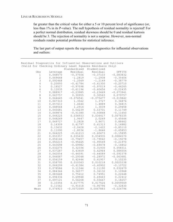
LINEAR REGRESSION MODELS
71
far greater than the critical value for either a 5 or 10 percent level of significance (or,less than 1% in its P-value). The null hypothesis of residual normality is rejected! Fora perfect normal distribution, residual skewness should be 0 and residual kurtosisshould be 3. The rejection of normality is not a surprise. However, non-normalresiduals render potential problems for statistical inference.
The last part of output reports the regression diagnostics for influential observationsand outliers:
Residual Diagnostics for Influential Observations and Outliers(Valid for Checking Ordinary Least Squares Residuals Only)
Standardized StudentizedObs Leverage Residual Residual DFFITS1 0.048570 -0.37556 -0.37103 -0.0838322 0.069668 -1.2819 -1.2938 -0.354063 0.092468 -1.2069 -1.2149 -0.387794 0.20093 -0.41784 -0.41300 -0.207105 0.18527 -0.97098 -0.97019 -0.462656 0.12035 -0.61196 -0.60656 -0.224357 0.088917 -0.23985 -0.23669 -0.0739418 0.063757 0.30955 0.30563 0.0797579 0.064645 -0.076541 -0.075477 -0.01984210 0.067310 1.3562 1.3727 0.3687611 0.057612 1.4644 1.4889 0.3681512 0.048564 1.2914 1.3039 0.2945813 0.045681 0.54239 0.53701 0.1174914 0.049876 -0.51380 -0.50848 -0.1165015 0.044225 0.036933 0.036417 0.007833516 0.048269 1.9447 2.0269 0.4564617 0.049727 3.2828 3.8671 0.8846218 0.14309 0.41797 0.41313 0.1688219 0.13632 -2.0428 -2.1422 -0.8511020 0.11090 -1.8036 -1.8646 -0.6585321 0.064225 -0.61213 -0.60673 -0.1589522 0.055357 0.035430 0.034935 0.008457023 0.056146 -0.79457 -0.79042 -0.1927824 0.050215 -0.95665 -0.95549 -0.2197025 0.043698 -0.69982 -0.69478 -0.1485226 0.032275 0.32336 0.31930 0.05831127 0.037287 0.43459 0.42964 0.08455428 0.042054 -0.44591 -0.44089 -0.09237829 0.046087 -0.29348 -0.28972 -0.06368130 0.056159 0.42446 0.41957 0.1023531 0.058795 0.010363 0.010218 0.002553832 0.064299 -0.41384 -0.40902 -0.1072233 0.078586 0.11346 0.11190 0.03267934 0.084366 0.36577 0.36132 0.1096835 0.083668 0.75412 0.74951 0.2264836 0.094336 0.69948 0.69443 0.2241237 0.097121 0.56208 0.55667 0.1825738 0.10356 0.017775 0.017526 0.005956939 0.11562 -0.91018 -0.90796 -0.32830
Mean 0.076923 -0.0072089 0.0067883 -0.024796

GAUSS PROGRAMMING FOR ECONOMETRICIANS AND FINANCIAL ANALYSTS
72
To check for influential observations and outliers, we first take a look at the column“Leverage,” which measures the influence of each observation on the regressors. Wecheck for leverage which is greater than 2×(K/N) where K is the number of estimatedcoefficients and N is the number of observations. In this case, 2×(K/N) = 2×(3/39) =0.154. Observations 4 and 5 (leverage 0.201 and 0.185 respectively) are quiteinfluential.
Standardized (or normalized) residuals should follow a standardized normaldistribution, provided that the Bera-Jarque test statistic confirms the distributionassumption. Unfortunately, this is not the case as shown by the test results above.Observations 17 and 19 (3.283 and –2.043 respectively) are greater than 2 standarderrors from the mean.
A more robust measure of outliers uses the studentized residuals (or standardizedpredicted residuals) which follows the Student’s t distribution with N-K-1 degrees offreedom. Given the critical value of 1.69 at a 5% level of significance, observations16, 17, 19, and 20 are candidates for outliers.
The last column, DFFITS, measures the contribution of each observation to theprediction of the model. The cut off value 2×(K/N)0.5 is suggested (that is, 0.555 in thecase of this Cobb-Douglas production model). The contribution of observations 17,19, and 20 are rather large.
Materials of this lesson on influential observations and outliers can be found in Judge,et. al. (1988) and Maddala (1988). In summary, for our study of the Cobb-Douglasproduction function, the model is sensitive to the use of data near the end of WorldWar II (i.e. observations 17, 19, and 20). The model may be better explained withoutthem.

IVDummy Variables
Dummy variables are widely used in econometrics to isolate sub-group effects in agiven sample. These sub-groups may be geographical regions, yearly quarters, gender,or periods in time. How dummy variables are used in regression estimation determinesin which way the sub-groups differ. The so-called dummy variables themselves remainvectors of ones and zeros. A one indicates the presence of a given characteristic, whilea zero indicates the absence. In most cases, one less dummy variable is used than thereare sub-groups. Estimated regressions from these sub-groups may have an additivedifference, a multiplicative difference, or a combined additive and multiplicativedifference. An additive difference refers to a parallel shift in the level of an estimatedregression. This shift is reflected in a change of the intercept term, while the othercoefficients remain unchanged. The slope coefficients will vary with their associatedmultiplicative dummy variables. The estimated changes in slope coefficients amongsub-groups are measured by the coefficients of multiplicative dummy variables. Acombined additive and multiplicative difference in sub-groups is achieved by a changein all coefficients, both intercept and slope terms.
Since entire chapters on dummy variables are written in fine academic referencesdetailing the interpretation of the results from using dummy variables, we will onlygive brief interpretations of our results. Instead, we explore in detail the generation ofdummy variables using GAUSS.
SeasonalityDetermining seasonal patterns in time series data is one application of dummyvariables. A new text data file named almon.txt will be used to study quarterlyseasonality. It has three variables. The first column is the date, in years and quarters(YEARQT). The second column is capital expenditures in millions of dollars (CEXP).The last column holds capital appropriations in millions of dollars(CAPP). The basicAlmon model describes the simple relationship between capital expenditures andappropriations as follows:
CEXP = β0 + β1 CAPP + ε
There are 60 observations in total, although Almon’s original study used the first 36observations from 1953 to 1961. Lesson 4.1 is devoted to the study of seasonal

GAUSS PROGRAMMING FOR ECONOMETRICIANS AND FINANCIAL ANALYSTS
74
differences with Almon’s quarterly time series on capital appropriations andexpenditures.
Does the use of dummy variables matter? Lesson 4.1 continues the hypothesis testingprocedure for significant differences in quarterly seasonality. It is achieved bycomparing regression results from restricted (without seasonal dummy variables) andunrestricted (with seasonal dummy variables) least squares.
In Lesson 4.2, the notorious problem of the “dummy variable trap” is discussed withan alternative use and interpretation of dummy variables in conjunction with theregression without intercept.
Lesson 4.1: Seasonal Dummy Variables
In this lesson, we introduce the use of additive dummy variables to remove seasonalityin Almon’s quarterly time series data.
First of all, seasonality implies that the best-fitting regression for each season (quarter)may be different. In other words, the intercept and slope terms that provide the best fitfor one quarter may not provide the best fit for different quarters. Before generatingthe seasonal dummy variable matrix, you need to have some idea of what it shouldlook like. It has a repeating set pattern of four columns, one for each quarter. Considerall 60 observations of time series data in almon.txt; a pattern of 0’s and 1’s is createdto represent one cycle of seasonality (that is, one year). The pattern is reshaped into a4-column matrix with the desired 60 rows:
pattern = 1 0 0 0,0 1 0 0,0 0 1 0,0 0 0 1;
D = reshape(pattern,60,4);q1 = D[.,1];q2 = D[.,2];q3 = D[.,3];
To avoid perfect collinearity with the constant column associated with the intercept,only three columns of the dummy variable matrix D will be used. That is, fourquarters are indicated with only three dummies: q1, q2, q3. Lesson 4.2 on dummyvariable trap explains why we must do this.
Now the model with three quarterly dummy variables is:
CEXP = β0 + β1 CAPP + δ1 Q1 + δ2 Q2 + δ3 Q3 + ε
Or, in four equations (one for each quarter) as follows:

DUMMY VARIABLES
75
Quarter 1: CEXP = (β0 + δ1) + β1 CAPP + εQuarter 2: CEXP = (β0 + δ2) + β1 CAPP + εQuarter 3: CEXP = (β0 + δ3) + β1 CAPP + εQuarter 4: CEXP = β0 + β1 CAPP + ε
We also will address the significance of seasonal differences in the model by testingthe three coefficients δ1, δ2, and δ3 are jointly equal to zero. This is a test procedurefor the presence of seasonality in the model we will examine later.
123
456
7891011121314
1516171819202122
/*** Lesson 4.1: Seasonal Dummy Variables*/use gpe2;output file = gpe\output4.1 reset;load almon[61,3] = gpe\almon.txt;
cexp = almon[2:61,2];capp = almon[2:61,3];qt = almon[2:61,1];
pattern = 1 0 0 0,0 1 0 0,0 0 1 0,0 0 0 1;
D = reshape(pattern,60,4);q1 = D[.,1]; @ quarterly seasonal dummies @q2 = D[.,2];q3 = D[.,3];
call reset;_names = "cexp", "capp", "q1", "q2", "q3";call estimate(cexp,capp~q1~q2~q3);_restr = 0 1 0 0 0,
0 0 1 0 0,0 0 0 1 0;
call estimate(cexp,capp~q1~q2~q3);end;
The estimation is carried out with three quarter dummy variables named q1, q2, andq3. The fourth quarter is the base case, and the coefficients of three dummy variablesidentify the additive differences from that of the fourth quarter, or the intercept term.
There are many ways to generate the dummy variables other than the suggested useof reshape command. A simple alternative is to rely on the quarter indicator qt,appearing in the first column of the data file almon.txt. Lines 7 through 14 of theabove program can be replaced by the following three lines:
q1 = (qt%10) .== 1;q2 = (qt%10) .== 2;q3 = (qt%10) .== 3;
The modulo division “%” returns the remainder of the integer division, and the

GAUSS PROGRAMMING FOR ECONOMETRICIANS AND FINANCIAL ANALYSTS
76
notation “.==” in GAUSS performs element by element equality comparison. Inother words, each line compares the last digit of qt to a given quarter, placing a onein the dummy variable if the comparison turns out to be true.
GAUSS has its own commands for creating dummy variables: dummy, dummybr,dummydn. The command dummy creates a matrix of dummy variables by breakinga vector of data into multiple groups. To make sense of this example, lines 7 through11 of the above program may be replaced by the following:
seasons = 1,2,3,4;D = dummy(qt%10, seasons);
Where the column vector seasons containing four quarter indicators is used tocompare with the last digit of the variable qt. GAUSS command dummy creates amatrix of four columns of dummy variables, D. It compares each data observation ofqt%10 to the breakpoints designated in vector seasons. If the data is in the rangedesignated, a one is placed in the corresponding element of matrix D, if not, a zero isplaced.
Running the program Lesson 4.1 will produce two sets of regression results in theoutput file output4.1. The first estimated model looks like this:
CEXP = 670.93 + 0.737 CAPP - 13.69 Q1 - 50.60 Q2 - 31.53 Q3s.e. (230.9) (0.053) (204.5) (204.3) (204.2)t-ratio 2.91 13.95 - 0.067 - 0.248 - 0.154
We can also write the estimated model as four separate equations, one for eachquarter:
Quarter 1: CEXP = (670.93 - 13.69) + 0.737 CAPPQuarter 2: CEXP = (670.93 - 50.60) + 0.737 CAPPQuarter 3: CEXP = (670.93 - 31.53) + 0.737 CAPPQuarter 4: CEXP = 670.93 + 0.737 CAPP
We have estimated the linear relationship between capital expenditures (CEXP) andappropriations (CAPP) with varying intercept terms to represent the seasonaldifferences in the model. Is there a real or significant difference among the fourestimated regression equations? Analyzing both the t-ratios and the P-values revealsthat the coefficients of dummy variables are not statistically significantly differentfrom zero. Furthermore, the partial regression values are very small for the dummyvariables. A more formal procedure is to test the hypothesis that all of the coefficientsof dummy variables are jointly equal to zero. The hypothesis is that δ1 = 0, δ2 = 0, andδ3 = 0 hold simultaneously. The GPE input control variable _restr (lines 18,19, and

DUMMY VARIABLES
77
20) defines Almon’s equation with the three quarterly dummy variables jointlyequaling zero.
_restr = 0 1 0 0 0,0 0 1 0 0,0 0 0 1 0;
Then, restricted least squares estimation is carried out in line 21. Here is the secondset of estimation results in which coefficients of three quarterly dummy variables arerestricted to zeros:
Least Squares Estimation------------------------Dependent Variable = CEXPEstimation Range = 1 60Number of Observations = 60Mean of Dependent Variable = 3092.4Standard Error of Dependent Variable = 1151.9
WARNING: Linear Restrictions Imposed.R-Square, AOV, SE, and t may not be reliable!Wald F-Test for Linear RestrictionsF( 3, 55) Prob>F
0.023130 0.99518
R-Square = 0.78006 R-Square Adjusted = 0.77626Standard Error of the Estimate = 544.88Log-Likelihood = -462.15Log Ammemiya Prediction Criterion (APC) = 12.681Log Akaike Information Criterion (AIC) = 12.734Log Schwarz Bayesian Information Criterion (BIC) = 12.908
Sum of Squares SS DF MSS F Prob>FExplained 6.1072E+007 1 6.1072E+007 205.70 9.9398E-021Residual 1.7220E+007 58 2.9689E+005Total 7.8291E+007 59 1.3270E+006
Variable Estimated Standard t-Ratio Prob PartialName Coefficient Error 58 DF >|t| RegressionCAPP 0.73684 0.051375 14.342 9.9398E-021 0.78006Q1 -6.1284E-014 0.00000 0.00000 0.00000 0.00000Q2 2.6290E-013 0.00000 0.00000 0.00000 0.00000Q3 -1.2079E-013 0.00000 0.00000 0.00000 0.00000CONSTANT 646.48 184.48 3.5044 0.00088917 0.17474
By comparing regression results from restricted (without seasonal dummy variables)and unrestricted (with seasonal dummy variables) least squares, the computed Waldtest statistic for the above three linear restrictions is a negligible 0.02, implyinginsignificant seasonal variation in the model. It is further confirmed with an extremelylarge P-value 0.99 of the test statistic. We can conclude safely that there is nodifference in the estimated Almon equations for the different quarters.

GAUSS PROGRAMMING FOR ECONOMETRICIANS AND FINANCIAL ANALYSTS
78
Lesson 4.2: Dummy Variable Trap
Here comes a technical question. When we estimated Almon’s model in Lesson 4.1,we only explicitly included three quarterly dummy variables in the regressionequation. Why would we drop the fourth dummy variable? If you keep the constantterm and use a dummy variable for each group, your program will generate an errormessage similar to the following:
C:\GAUSS\SRC\GPE2.SRC(1250) : error G0121 : Matrix not positive definiteCurrently active call: _lsqest [1250]
This condition is called the “dummy variable trap”. The dummy variable trap gets justabout everyone at some time. Understanding how the dummy variable trap happenswill make avoiding it easier. Remember that a typical regression equation contains aconstant vector of ones associated with the intercept coefficient. Now, if there is adummy variable for each group, summing all the dummy variables together equalsone. The problem of perfect collinearity exists! Dropping one dummy variable is notthe only solution to stay out of the “trap”. The alternative is to include all dummyvariables but to estimate the regression without the intercept term. In GPE, regressionestimation without intercept is carried out by setting the input control variable:
_const = 0;
The following program is a slightly modified version of the previous program. Itincludes all four quarterly dummy variables, but the model is estimated without theintercept term.
123
456
7891011
1213141516
/*** Lesson 4.2: Dummy Variable Trap*/use gpe2;output file = gpe\output4.2 reset;load almon[61,3] = gpe\almon.txt;
cexp = almon[2:61,2];capp = almon[2:61,3];qt = almon[2:61,1];
pattern = 1 0 0 0,0 1 0 0,0 0 1 0,0 0 0 1;
D = reshape(pattern,60,4);
call reset;_const = 0; @ regression without intercept @_names = "cexp","capp","q1","q2","q3","q4";call estimate(cexp,capp~D);end;

DUMMY VARIABLES
79
Run this program, and refer to the output file output4.2 for details. The importantcatch is the statement of line 13:
_const = 0;
Without it, you will fall into the “dummy variable trap”! The estimated model can besummarized as follows:
CEXP = 0.737 CAPP + 657.23 Q1 + 620.32 Q2 + 639.40 Q3 + 670.93 Q4s.e. (0.053) (222.4) (222.7) (222.4) (230.9)t-ratio 13.95 2.95 2.74 2.80 2.91
The interpretation of the coefficients associated with four quarter dummy variables isdirectly reflected as the intercept values of each equation:
Quarter 1: CEXP = 657.23 + 0.737 CAPPQuarter 2: CEXP = 620.32 + 0.737 CAPPQuarter 3: CEXP = 639.40 + 0.737 CAPPQuarter 4: CEXP = 670.93 + 0.737 CAPP
A careful eye will see that these results are the same as those of the first regressionequation in Lesson 4.1 using 3 dummies and a constant term.
Structural ChangeIn the next lesson, we will use a dummy variable approach to estimate and test forstructural change previously studied in the production function of Lesson 3.5. Recallthat a simple Cobb-Douglas production function was estimated using time series of U.S. real output (X), labor (L) and capital (K) inputs obtained from the data file cjx.txt.The question was, is there a change in both intercept and slope terms during post-warexpansion after 1948? In Lesson 3.5, a Chow test was formulated and performed withtwo separate samples: 1929-1948 and 1949-1967. The alternative approach is to use adummy variable for sample separation, and check for the difference in intercept andslope terms of the regression for each sub-sample. To check for the interceptdifference, the use of an additive dummy variable would suffice. To check for theslope difference, a multiplicative dummy variable associated with each explanatoryvariable should be used.
Lesson 4.3: Testing for Structural Change: Dummy Variable Approach
When breaking the time series data in cjx.txt into two sub-groups, only one dummyvariable named D is created (one less than the number of sub-groups). D is a vectorwhose entries are equal to zero for all observations in the first time period (1929-1948), and one for all observations in the second period (1949-1967). One way to

GAUSS PROGRAMMING FOR ECONOMETRICIANS AND FINANCIAL ANALYSTS
80
create D is to compare a given vector available in the original time series to a setvalue. In this lesson we create a dummy variable D by comparing each observation inthe vector YEAR to the value 1948. For every observation greater than 1948 D is setto one, otherwise D is set to zero. Notice that the dot (.) before the ( > ) meanselement-by-element greater-than comparison:
D = year.>1948;
If the number of continuing observations designed for the base and alternativesituations are known, concatenating a vector of zeros vertically to a vector of ones isa simple method of creating the dummy variable D. In this case,
D = zeros(20,1)|ones(19,1);
123
4567
8910
1112131415161718
/*** Lesson 4.3: Testing for Structural Change** Dummy Variable Approach*/use gpe2;output file = gpe\output4.3 reset;load data[40,6] = gpe\cjx.txt;
year = data[2:40,1];X = ln(data[2:40,2]);L = ln(data[2:40,3]);K = ln(data[2:40,5]);
D = year.>1948;DL = D.*L;DK = D.*K;
call reset;_names = "X","L","K","DL","DK","D";call estimate(X,L~K~DL~DK~D);_restr = 0 0 1 0 0 0,
0 0 0 1 0 0,0 0 0 0 1 0;
call estimate(X,L~K~DL~DK~D);end;
Line 8 creates the additive dummy variable named D. Lines 9 and 10 use D to set upmultiplicative dummy variables in association with the other two explanatoryvariables L and K, respectively. Thus, for entries of D equal to one, the correspondingentry in DL equals L and the corresponding entry in DK equals K. Otherwise, theentries of DL and DK are zeros. The three dummy variables, one additive and twomultiplicative, are added to estimate in line 13. In this example, our model can bewritten in two ways. It may be written with two separate regressions, one for yearsbefore 1948 and one for the years after. This example demonstrates how to constructboth situations into one combined regression as follows:
X = β0 + β1 L + β2 K + δ0 D + δ1 DL + δ2 DK + ε

DUMMY VARIABLES
81
When D equals zero (that is, for the period 1929-1948), we have what is called thebase case. When D equals one (that is, 1949-1967), the estimated coefficients of thedummy variables are added to the estimated coefficients of the independent variablesincluding the constant vector. In other words,
For 1929-1948, X = β0 + β1 L + β2 K + ε;For 1949-1967, X = (β0 + δ0) + (β1 + δ1) L + (β2 + δ2)K + ε
Run the program so that we can check out the first estimated regression from theoutput:
Least Squares Estimation------------------------Dependent Variable = XEstimation Range = 1 39Number of Observations = 39Mean of Dependent Variable = 5.6874Standard Error of Dependent Variable = 0.46096
R-Square = 0.99518 R-Square Adjusted = 0.99445Standard Error of the Estimate = 0.034338Log-Likelihood = 79.407Log Ammemiya Prediction Criterion (APC) = -6.5999Log Akaike Information Criterion (AIC) = -6.6023Log Schwarz Bayesian Information Criterion (BIC) = -6.3464
Sum of Squares SS DF MSS F Prob>FExplained 8.0355 5 1.6071 1362.9 3.2814E-037Residual 0.038911 33 0.0011791Total 8.0744 38 0.21248
Variable Estimated Standard t-Ratio Prob PartialName Coefficient Error 33 DF >|t| RegressionL 1.6167 0.15690 10.304 7.6101E-012 0.76288K 0.21967 0.17266 1.2723 0.21217 0.046758DL -0.60772 0.37578 -1.6172 0.11535 0.073433DK 0.35942 0.21672 1.6584 0.10670 0.076935D 1.5595 1.2876 1.2111 0.23444 0.042559CONSTANT -4.0576 0.26822 -15.128 2.1113E-016 0.87397
Interpreting the output gives us the estimated model;
X = - 4.06 + 1.62 L + 0.22 K - 0.61 DL + 0.36 DK + 1.56 Ds.e. (0.27) (0.16) (0.17) (0.38) (0.22) (1.29)t-ratio - 15.1 10.3 1.27 - 1.62 1.66 1.21
In terms of two separate samples:
For 1929 - 1948, X = -4.06 + 1.62 L + 0.22 K (base case)

GAUSS PROGRAMMING FOR ECONOMETRICIANS AND FINANCIAL ANALYSTS
82
For 1949 - 1967, X = (-4.06 + 1.56) + (1.62 -0.61) L + (0.22 + 0.36) K or, X = -2.50 + 1.01 L + 0.58 K
One look at t-ratios and P-values tells us that the dummy variables are not statisticallysignificant. To test for the structural change, we need to verify that the coefficients ofboth additive and multiplicative dummy variables are all zero. In other words, wemust show that δ0 = 0, δ1 = 0, and δ2 = 0 jointly. The GPE input control variable_restr, defines these three dummy variables in a 3 by 6 matrix as shown in lines 14through 16:
_restr = 0 0 1 0 0 0,0 0 0 1 0 0,0 0 0 0 1 0;
Line 17 estimates the restricted model (restricting all coefficients associated withdummy variables to zeros) in which no structural change is assumed. Here is the resultof the restricted least squares estimation:
Least Squares Estimation------------------------Dependent Variable = XEstimation Range = 1 39Number of Observations = 39Mean of Dependent Variable = 5.6874Standard Error of Dependent Variable = 0.46096
WARNING: Linear Restrictions Imposed.R-Square, AOV, SE, and t may not be reliable!Wald F-Test for Linear RestrictionsF( 3, 33) Prob>F
1.2639 0.30275
R-Square = 0.99463 R-Square Adjusted = 0.99433Standard Error of the Estimate = 0.034714Log-Likelihood = 77.286Log Ammemiya Prediction Criterion (APC) = -6.5781Log Akaike Information Criterion (AIC) = -6.4936Log Schwarz Bayesian Information Criterion (BIC) = -6.2376
Sum of Squares SS DF MSS F Prob>FExplained 8.0310 2 4.0155 3332.2 1.3921E-041Residual 0.043382 36 0.0012051Total 8.0744 38 0.21248
Variable Estimated Standard t-Ratio Prob PartialName Coefficient Error 36 DF >|t| RegressionL 1.4508 0.083228 17.431 3.9260E-019 0.89407K 0.38381 0.048018 7.9930 1.7130E-009 0.63960DL -5.1890E-012 0.00000 0.00000 0.00000 0.00000DK 2.3426E-012 0.00000 0.00000 0.00000 0.00000D 1.6888E-011 1.7378E-007 9.7182E-005 0.99992 2.6234E-010CONSTANT -3.9377 0.23700 -16.615 1.8332E-018 0.88464

DUMMY VARIABLES
83
Comparing the result of Chow test presented in Lesson 3.5, to the above output showsan identical computed Wald F-test statistic of 1.27 for three linear restrictions ondummy variables. In other words, based on the Cobb-Douglas log specification of theproduction function, there is no reason to believe that there was a structural change inoutput productivity between the years of 1929 - 1967. Both Lesson 3.5 (sampleseparation approach) and Lesson 4.3 (dummy variable approach) reach the sameconclusion. However, for a careful eye, there are subtle differences in the estimatedstandard errors and t-ratios for the regression coefficients obtained from these twoapproaches. Why?


VMulticollinearity
Multicollinearity is a data problem due to a group of highly correlated explanatoryvariables used in the regression equation. The consequence of multicollinearity is theresulting large standard errors of the coefficient estimates. It is conceived that thereare too many explanatory variables and some of them may not be needed. Then thequestion is how to identify and treat the irrelevant explanatory variables in theregression.
The famous Longley data is known for the problem of multicollinearity. Instead ofconstructing a meaningful model, we will demonstrate a hypothetical relationship withthe dependent variable (EM), regressed against a set of four other variables (YEAR,PGNP, GNP, and AF).
Detecting MulticollinearityGiven the regression equation:
EM = β0 + β1 YEAR + β2 PGNP + β3 GNP + β4 AF + ε
the focus of this chapter is to examine how closely the four explanatory variables:YEAR, PGNP, GNP, and AF are related. Lessons 5.1, 5.2, and 5.3 address thetechniques of detecting multicollinearity. These include: condition number andcorrelation matrix (Lesson 5.1), Theil’s measure of multicollinearity (Lesson 5.2), andvariance inflation factors (Lesson 5.3).
Lesson 5.1: Condition Number and Correlation Matrix
We have seen the regression outputs from previous lessons, which include a columnof partial correlation coefficients. Technically, it is computed using the formula:
t2
t2+DF
where t is the vector of t-ratios of coefficient estimates, and DF is the degrees offreedom of the estimated regression. The partial correlation coefficient, as its namesuggests, measures the marginal or partial contribution of the designated variable

GAUSS PROGRAMMING FOR ECONOMETRICIANS AND FINANCIAL ANALYSTS
86
when the influence of other variables are already considered. The smaller the partialcorrelation coefficient, the less important the variable would be in the regressionequation. It is a useful approach to identify the irrelevant variable as a candidate fordeletion.
Another useful tool to check for the problem of multicollinearity is the datacorrelation matrix, which describes the simple pair-wise correlation among all thevariables used in the regression. The built-in GAUSS command corrx can doexactly that, but the GPE package offers the convenience of a data correlation matrixby setting the following input control variable:
_corr = 1;
The condition number of a normalized data matrix of explanatory variables iscomputed as well. The normalization is necessary so that the condition number isindependent of the unit of measurement for each variable. A large condition numberindicates multicollinearity. Large values of pair-wise correlation coefficients may hintat the source of the problem.
Using Longley data, the following program estimates the model with the dependentvariable (EM) regressed against a set of four other variables (YEAR, PGNP, GNP,and AF). The problem of multicollinearity is detected by examining the partialregression coefficients, as well as the condition number and correlation matrix of theexplanatory variables.
1234
56789
1011121314
/*** Lesson 5.1: Condition Number and Correlation Matrix*/use gpe2;output file = gpe\output5.1 reset;load data[17,7] = gpe\longley.txt;data = data[2:17,.];
year = data[.,1];pgnp = data[.,2];gnp = data[.,3];af = data[.,5];em = data[.,7];
call reset;_corr = 1; @ cond# and correlation matrix @_names = "em","year","pgnp","gnp","af";call estimate(em,year~pgnp~gnp~af);end;
Running the above program returns the following output:

MULTICOLLINEARITY
87
Least Squares Estimation------------------------Dependent Variable = EMEstimation Range = 1 16Number of Observations = 16Mean of Dependent Variable = 65317.Standard Error of Dependent Variable = 3512.0
R-Square = 0.97352 R-Square Adjusted = 0.96389Standard Error of the Estimate = 667.34Log-Likelihood = -123.76Log Ammemiya Prediction Criterion (APC) = 13.279Log Akaike Information Criterion (AIC) = 13.257Log Schwarz Bayesian Information Criterion (BIC) = 13.498
Sum of Squares SS DF MSS F Prob>FExplained 1.8011E+008 4 4.5028E+007 101.11 1.3458E-008Residual 4.8987E+006 11 4.4534E+005Total 1.8501E+008 15 1.2334E+007
Variable Estimated Standard t-Ratio Prob PartialName Coefficient Error 11 DF >|t| RegressionYEAR -576.46 433.49 -1.3298 0.21049 0.13850PGNP -19.768 138.89 -0.14233 0.88940 0.0018381GNP 0.064394 0.019952 3.2275 0.0080515 0.48638AF -0.010145 0.30857 -0.032878 0.97436 9.8262E-005CONSTANT 1.1691E+006 8.3590E+005 1.3986 0.18949 0.15098
Condition Number of Explanatory Variables = 15824.Correlation Matrix of Dependent and Explanatory VariablesEM 1.0000YEAR 0.97133 1.0000PGNP 0.97090 0.99115 1.0000GNP 0.98355 0.99527 0.99159 1.0000AF 0.45731 0.41725 0.46474 0.44644 1.0000
EM YEAR PGNP GNP AF
With the exception of the variable GNP, small partial regression coefficients arestrong indications of irrelevant explanatory variables. The added information from theuse of the input control variable _corr = 1 (line 11) includes the condition numberand correlation matrix of the explanatory variables. The correlation coefficientsbetween the dependent variable and each independent variable are given in the firstcolumn of the correlation matrix. These measure the individual effect of eachindependent variable on the dependent variable. With the exception of the variableAF, the explanatory variables have a rather high correlation with the dependentvariable. However, these variables are also highly correlated among themselves, asseen from the rest of the correlation matrix. In addition, the condition number ofexplanatory variables is extremely large, suggesting severe multicollinearity for thisset of variables.

GAUSS PROGRAMMING FOR ECONOMETRICIANS AND FINANCIAL ANALYSTS
88
Lesson 5.2: Theil’s Measure of Multicollinearity
Similar to the concept of partial regression coefficients, Theil’s measure ofmulticollinearity uses the R-square from multiple partial regressions to determine ifmulticollinearity is present in a regression equation.
Theil’s measure of multicollinearity is a formula derived from
R2 – ∑j=2,…,K (R2 – R-j2)
where R2 is the R-square (that is, coefficient of determination) of the full model,including all explanatory variables. R-j
2 is the R-square of the same regression modelexcluding the j-th explanatory variable. Therefore, the difference R2 - R-j
2 measuresthe net contribution of the j-th explanatory variable in terms of R-square. K is thenumber of explanatory variables of the full regression, in which the first one is theconstant term. Notice that the index j for summation does not count the constant term.The ideal case of no multicollinearity is that Theil’s measure equals or is close to zero.
The first regression in the following program (lines 10-13) estimates the full modelwith dependent variable (EM) on a set of four independent variables (YEAR, PGNP,GNP, and AF). The rest of the program (lines 14-33) estimates four regressionequations, each corresponds to the partial model with one of the independent variablesremoved. The R-squares from the full model and from the four partial models are thenused to compute the Theil’s measure of multicollinearity.
Instead of showing the lengthy results of each regression estimation, we explain theuse of output control variables in GPE for keeping track of the information from eachof the regression runs. The use of an output control variable is first introduced in line13. In GPE, output control variables take on new values each time estimate orforecast is called. An output control variable is identified with a name beginningwith a double underscore ( __ ). For example, __r2 is the value of R-squarecomputed in the previous estimation. Therefore, in line 13, assigning __r2 to avariable named r2 allows us to use that value later in the program. See Appendix Afor a complete list of output control variables available in GPE.
123456789
/*** Lesson 5.2: Theil’s Measure of Multicollinearity*/use gpe2;output file = gpe\output5.2 reset;load data[17,7] = gpe\longley.txt;data = data[2:17,.];year = data[.,1];pgnp = data[.,2];gnp = data[.,3];af = data[.,5];em = data[.,7];

MULTICOLLINEARITY
89
101112131415161718192021222324252627282930313233
call reset;_names = "em","year","pgnp","gnp","af";call estimate(em,year~pgnp~gnp~af);r2 =__r2;call reset;print"Partial Regression 1: EM = PGNP GNP AF";_names = "em","pgnp","gnp","af";call estimate(em,pgnp~gnp~af);r2x1 = __r2;print"Partial Regression 2: EM = YEAR GNP AF";_names = "em","year","gnp","af";call estimate(em,year~gnp~af);r2x2 = __r2;print"Partial Regression 3: EM = YEAR PGNP AF";_names = "em","year","pgnp","af";call estimate(em,year~pgnp~af);r2x3 = __r2;print"Partial Regression 4: EM = YEAR GNP PGNP";_names = "em","year","gnp","pgnp";call estimate(em,year~gnp~pgnp);r2x4 = __r2;print "Theil's Measure of Multicollinearity =";;print r2-sumc(r2-(r2x1|r2x2|r2x3|r2x4));end;
From four partial regressions, we repeat the use of output variable __r2, to keep trackof the R-square of each regression. By renaming each __r2 and subtracting it from theR-square of the full model, these net differences are concatenated and then summedusing a GAUSS command sumc (see line 32). Running the program, the outputdisplays the results of all the regressions before the line:
Theil's Measure of Multicollinearity = 0.94414
In summary, the near unity of the Theil’s measure confirms the problem ofmulticollinearity.
Lesson 5.3: Variance Inflation Factors (VIF)
Relating to the correlation matrix of explanatory variables, Variance Inflation Factors(VIF) is the ratio of a variable’s actual variance to the perfect variance of zerocollinearity. Variance Inflation Factors (VIF) is defined as:
1 1- Rj
2
It can be used to detect multicollinearity, where Rj2 is the R-square from regressing the
j-th explanatory variable on all the other explanatory variables. A near unity Rj2 and
hence a high value of VIF indicates a potential problem of multicollinearity with the j-th variable.

GAUSS PROGRAMMING FOR ECONOMETRICIANS AND FINANCIAL ANALYSTS
90
The following program computes Variance Inflation Factors (VIF) for eachexplanatory variable through a set of four auxiliary regressions similar to theprocedure used in computing Theil’s measure of multicolinearity.
123456789101112131415161718192021222324252627282930313233343536373839
/*** Lesson 5.3: Variance Inflation Factors (VIF)*/use gpe2;output file = gpe\output5.3 reset;load data[17,7] = gpe\longley.txt;data = data[2:17,.];year = data[.,1];pgnp = data[.,2];gnp = data[.,3];af = data[.,5];em = data[.,7];call reset;print "Aux Regression 1: YEAR = PGNP GNP AF";y = year;x = pgnp~gnp~af;_names = "year","pgnp","gnp","af";call estimate(y,x);r2x1 = __r2;print "Aux Regression 2: PGNP = YEAR GNP AF";y = pgnp;x = year~gnp~af;_names = "pgnp","year","gnp","af";call estimate(y,x);r2x2 = __r2;print "Aux Regression 3: GNP = YEAR PGNP AF";y = gnp;x = year~pgnp~af;_names = "gnp","year","pgnp","af";call estimate(y,x);r2x3 = __r2;print "Aux Regression 4: AF = YEAR GNP PGNP";y = af;x = year~gnp~pgnp;_names = "af","year","gnp","pgnp";call estimate(y,x);r2x4 = __r2;r2=r2x1|r2x2|r2x3|r2x4;print "Variance Inflation Factors:";print " Model R-Square VIF";;print seqa(1,1,4)~r2~(1/(1-r2));end;
The first part of the program performs four auxiliary regression estimations. Eachcorresponds to the regression of one selected explanatory variable against the rest ofthe others. Only the R-squares from the four estimated regressions are of interest incomputing the VIF. First, these values are retained using the output variable __r2,then they are concatenated into a vector (line 35) for calculating the VIF of eachvariable (line 38). Based on the R-square measure of each auxiliary regression, VIFfor each explanatory variable is reported as follows:

MULTICOLLINEARITY
91
Variance Inflation Factors:Model R-Square VIF1.0000 0.99303 143.462.0000 0.98678 75.6713.0000 0.99245 132.464.0000 0.35616 1.5532
Again, all explanatory variables except variable AF (Model 4) have higher thannormal values of VIF indicating a severe problem of multicollinearity.
Correction for MulticollinearityWhat to do with the problem of multicollinearity? Beside tweaking with theappropriate explanatory variables and data transformation, techniques such as ridgeregression and principal components are suggested in the literature. The ridgeregression approach seeks to find a set of “stable” coefficient estimates with a“shrinkage parameter”, while the principal components approach is to extract asmaller number of independent variables (principal components) that explain most ofthe variation of regressors. The resulting coefficient estimates from these methods arebiased and difficult to interpret, even though they may be more precise (efficient) thantheir ordinary least squares counterparts. Since multicollinearity is a data problem,data adjustment and variable transformation should be considered in favor ofmechanical correction methods for estimation. Nevertheless, the following lessonillustrates the correction mechanics of ridge regression and principal components.
Lesson 5.4: Ridge Regression and Principal Components
GPE’s estimate procedure does not offer either ridge regression or principalcomponents. Given the estimates obtained from ordinary least squares, however, it israther straightforward to implement the computation of ridge regression and principalcomponents. Many standard econometrics textbooks outline the formula. Forexamples, see Judge, et. al. (1988, Chap. 21) and Greene (1999, Chap. 6).
Given a shrinkage parameter of r>0, the coefficient estimates br of ridge regression arerelated to the ordinary least squares estimate b of β in the regression equation Y = Xβ+ ε as follows:
br = (I + r(X’X)-1)-1b
Therefore, the corresponding estimated variance-covariance matrix Var(br) is:
Var(br) = (I + r(X’X)-1)-1Var(b) (I + r(X’X)-1)-1

GAUSS PROGRAMMING FOR ECONOMETRICIANS AND FINANCIAL ANALYSTS
92
= s2(I + r(X’X)-1)-1X’X (I + r(X’X)-1)-1
Where Var(b)is the estimated variance-covariance matrix and s2 is the regressionvariance of the ordinary least squares estimates. By varying the shrinkage parameter r,we can find the most “stable” coefficient estimates.
The method of principal components is to extract sufficient variation of independentvariables to explain the dependent variable of a regression equation. Let X be the datamatrix of the explanatory variables, including the constant term. Principal componentsof X are derived from linear combinations of characteristic vectors of X’X. We willuse only the principal components which satisfy a minimum size requirement of thecharacteristic roots of X’X. Let V be the matrix of such characteristic vectors. Then,the coefficient estimates of principal components bpc are related to the least squaresestimates b as follows:
bpc = VV’b
and the corresponding estimated variance-covariance matrix Var(bpc) is:
Var(bpc) = (VV’)Var(b)(VV’)
Lesson 5.4 is a GAUSS program which implements the ridge regression and principalcomponents based on the hypothetical regression equation with the Longley data asdescribed in the previous Lessons 5.1 to 5.3. After obtaining the ordinary least squaresresult, we introduce several GAUSS commands to perform ridge regression andprincipal components estimation. For detailed explanations of the GAUSS commandsused therein, refer to the GAUSS Command References or consult the on-line Helpmenu.
123456789101112
13
14
/*** Lesson 5.4: Ridge Regression and Principal Components*/use gpe2;output file = gpe\output5.4 reset;load data[17,7] = gpe\longley.txt;data = data[2:17,.];year = data[.,1];pgnp = data[.,2];gnp = data[.,3];af = data[.,5];em = data[.,7];call reset;_names = "em","year","pgnp","gnp","af";call estimate(em,year~pgnp~gnp~af);
/* explanatory variables including constant */x = year~pgnp~gnp~af~ones(rows(year),1);/* ridge regression */r=0.3;

MULTICOLLINEARITY
93
151617181920
212223242526272829
a = invpd(eye(cols(x))+r*invpd(x'x));br = a*__b;vbr = a*__vb*a';print "Ridge Regression Model:";print " Coefficient Std Error";;print br~sqrt(diag(vbr));
/* Principal Components */@ compute char. roots and vectors of X'X @r,v=eigrs2(x'x);v = selif(v',r.>0.1)';bpc = v*v'__b;vbpc = v*v'__vb*v*v';print;print "Principal Components Model:";print " Coefficient Std Error";;print bpc~sqrt(diag(vbpc));end;
First we estimate the equation using ordinary least squares (lines 10-12), then fromline 13 on we focus on the data matrix of explanatory variables including the constantterm, to perform ridge regression and principal components. Ridge regression isobtained for a shrinkage parameter of 0.3 (lines 14-20). We could try several smallpositive values for a shrinkage parameter to find the most “stable” coefficientestimates. The following output is the result of ridge regression:
Ridge Regression Model:Coefficient Std Error
29.750 3.8485-99.844 124.850.043571 0.0132330.16452 0.281912.5061 1.7759
We continue on to perform the principal components method (lines 21-28). Tocompute the principal components of the data matrix X of regressors, we pick only thecharacteristic vectors which correspond to the characteristic roots of X’X with valuesgreater than 0.1 (line 22). We notice that the computation of characteristic roots andvectors and therefore the result of principal components are sensitive to the scale ofmeasurement used in the data matrix.
The resulting estimates of principal components are:
Principal Components Model:Coefficient Std Error
29.784 3.8893-100.92 126.190.043684 0.0133720.16499 0.282020.022451 0.010768

GAUSS PROGRAMMING FOR ECONOMETRICIANS AND FINANCIAL ANALYSTS
94
As we can see from the above example, the computation of ridge regression andprincipal components is easy, but the interpretation of the resulting coefficientestimates will be difficult.

VI Nonlinear Optimization
To find an optimal (maximal or minimal) solution of a scalar-valued function is at thecore of econometric methodology. The technique of least squares estimation is anexample of solving the nonlinear “sum-of-squares” objective function. For a linearregression model, the exact solution is derived using the analytical formula of matrixalgebra. However, the problem may be more complicated if the regression equation isnonlinear in the parameters. In this case, approximation or iterative methods ofnonlinear optimization will be necessary. We will consider only the case ofunconstrained optimization. In most cases, simple equality constraints can besubstituted into the objective function so that the problem is essentially theunconstrained one. Nonlinear optimization with inequality constraints is difficult,though not impossible.
From elementary differential calculus, an optimal solution can be found by setting thefirst derivatives (gradient) of the objective function with respect to the function’svariables equal to zero and solving for the variables. Then to verify a minimum(maximum), the second derivatives matrix (hessian) must be positive (negative)definite. When the functional form is simple, the analytical approach of working outthe derivatives is useful. The techniques of numerical approximation and iteration aremore practical for solving large and complex optimization problems. GPE offerspractical techniques for finding numeric solutions of a general nonlinear objectivefunction.
Although the nonlinear optimization of GPE is designed with statistical oreconometric problems in mind, it can be used for solving mathematical functions aswell. The first step is to define the objective function, mathematical or statistical. Thenext step is to solve the function through numerical optimization by calling theprocedure estimate.
Solving Mathematical FunctionsWithout going into the details of optimization theory, we first describe how to defineand write an objective function suitable for solving its optimum (or optima). Recallthat a simple function can be defined with a single-line fn statement in GAUSS (seeChapter II). Since GPE is designed for econometric or statistical problem-solving, an

GAUSS PROGRAMMING FOR ECONOMETRICIANS AND FINANCIAL ANALYSTS
96
objective function is defined with a set of sample data and a vector of unknownparameters. Typically a one-line fn or multi-line proc statement is declared as:
fn FunctionName(Data,Parameters) = …;
or
proc FunctionName(Data,Parameters);…endp;
Where FunctionName is the name of the function, Data is the sampleobservations of data series, and Parameters are the parameters or coefficients ofthe function. For a statistical model, both Data and Parameters are used to definethe function FunctionName. For a mathematical function only the Parametersmatter, therefore Data can be set to 0 (or a dummy value) in this case.
The actual computation of solving the function FunctionName is carried out bycalling the procedure estimate, as follows:
call estimate(&FunctionName,Data);
Where &FunctionName denotes the code address (holding place) of the functionFunctionName we declared earlier, which is defined with Data (a set of sampledata) and Parameters (a vector of initial values of parameters).
Using GPE for nonlinear functional optimization (or estimation), the following inputcontrol variables are required:
• _nlopt• _b• _iter
The GPE input control variable _nlopt defines the type of optimization probleminvolved. _nlopt=0 indicates a minimization problem, while _nlopt=1 indicatesa maximization problem. Since numerical iteration is used for solving a nonlinearmodel, the solution found can be at best a local one. The input variable _b providesthe initial guess of parameters as the starting point of iterations. Different startingvalues of _b may lead to different (local) solutions. In an effort to find a globalsolution for the function, several different values of _b should be tried. The variable_iter sets the maximal number of iterations allowed for a particular problem.Usually we keep _iter low for testing the function. When the function is debuggedand ready for solving, _iter should be set large enough to ensure the convergence ofan iterative solution.

NONLINEAR OPTIMIZATION
97
Calling the procedure estimate for nonlinear model estimation (or optimization) issimilar to the case of the linear regression model. The differences are that undernonlinear estimation or optimization, the first argument of estimate is now anaddress for the objective function and the second argument (for the data matrix) ismore forgiving in its structure. Remember that the objective function must be definedwith the data and parameters before calling the estimate procedure.
Lesson 6.1: One-Variable Scalar-Valued Function
Consider a scalar-valued function of one variable,
f(x) = ln(x) – x2.
The single maximum of f(x) is found at x = ½ . First we translate the mathematicalfunction f(x) into a GAUSS fn statement as in line 3 of the following program:
12
3
4567
89
/*** Lesson 6.1: One-Variable Scalar-Valued Function** f(x) = ln(x) – x^2*/use gpe2;output file=output6.1 reset;
fn f(data,x)=ln(x)-x^2;
call reset;_nlopt=1;_iter=100;_b=0.5;
call estimate(&f,0);end;
Line 5 indicates the maximization problem involved, and line 6 sets the iteration limitfor finding the solution. The estimation (maximization, in particular) of function fstarts with the initial value of x at 0.5 as shown in line 7. The GPE input variable _bcontrols the starting value of iteration. Notice that here we do not use sample data orparameter names in defining the function and maximization. Running the above lessonprogram, we obtain the following result:
Non-Linear Optimization: Maximization Problem---------------------------------------------Number of Parameters = 1
Maximum Number of Iterations = 100Step Size Search Method = 0Convergence Criterion = 0Tolerance = 0.001

GAUSS PROGRAMMING FOR ECONOMETRICIANS AND FINANCIAL ANALYSTS
98
Initial Result:Function Value = -0.94315Parameters = 0.50000
Using Steepest-Ascent AlgorithmIteration = 1 Step Size = 0.2500 Value = -0.85018Parameters = 0.75000Iteration = 2 Step Size = 0.5000 Value = -0.84991Parameters = 0.66667Iteration = 3 Step Size = 0.2500 Value = -0.84658Parameters = 0.70833Iteration = 4 Step Size = 0.5000 Value = -0.84658Parameters = 0.70588Iteration = 5 Step Size = 0.2500 Value = -0.84657Parameters = 0.70711Iteration = 6 Step Size = 0.2500 Value = -0.84657Parameters = 0.70711
Final Result:Iterations = 6 Evaluations = 38Function Value = -0.84657Parameters = 0.70711Gradient Vector = -4.2549e-006Hessian Matrix = -4.0000
Starting at x = 0.5 with function value – 0.94315, it takes six iterations to reach theconvergence of a solution. The solution 0.70711 is indeed a maximum with functionvalue – 0.84657, where the gradient is almost zero at – 4.2549e-06 and the hessian isnegative at – 4.0.
You may want to define the function’s analytical derivatives and use them forsolving the function. For this example, they are:
fn f1(data,x) = 1/x – 2*x;fn f2(data,x) = -1/(x^2) – 2;
The functions f1 and f2 are the first and second derivatives of f, respectively. Itmay be necessary to write a multi-line procedure for the derivatives of a morecomplicated function. To solve the function with analytical derivatives, justhorizontally concatenate the function and derivatives together as a row vector andput them in the first argument of the procedure estimate as below:
call estimate(&f~&f1~&f2,0);
There is no need to use both first and second derivatives. Using only the firstderivative will work. The use of analytical derivatives will speed up the computationand increase the numerical precision of the solution. However, for a complicatedfunction, it is often a difficult task to write and code the analytical formula ofderivatives.

NONLINEAR OPTIMIZATION
99
The bare-bones program of Lesson 6.1 does not take advantage of the many optionsavailable in GPE to fine tune the optimization process. For a simple problem, as theone shown above, the default settings of optimization method (i.e., steepest-ascentmethod) and convergence criteria (i.e., convergence in function value and solutionrelative to the tolerance level of 0.001) may be acceptable.
We now explain some of the GPE input control variables, which provide the optionsto select one of many optimization methods and control its behavior in order to findthe optimal solution for a more complicated and difficult function. These controlvariables are:
• _method• _step• _conv• _tol• _restart
By default, _method is set to 0 if we do not specify any method of optimization inthe program. For a mathematical problem, the default method is the steepest descentor ascent method. For a statistical model, it is the Gauss-Newton method for nonlinearleast squares, or steepest descent method for maximum likelihood estimation. Thefollowing lists the more sophisticated optimization methods available :
_method=1 Broyden-Fletcher-Goldfarb-Shanon (BFGS) quasi-Newton method._method=2 Davidon-Fletcher-Powell (DFP) quai-Newton method._method=3 Greenstadt method._method=4 Newton-Raphson method._method=5 Quadratic-hill climbing method._method=6 Modified quadratic-hill climbing method.
All the optimization or estimation methods should be combined with a line search todetermine the step size of optimization for each iteration. The default line searchmethod is a simple cut back method (_step=0). Setting _step=1, uses thequadratic step size in search. Readers interested in a more detailed discussion andcomparison of different optimization methods should check the references (e.g.,Quandt, 1983; Judge, et. al., 1985, Appendix B; Greene, 1999, Chapter 5) for details.
The other optional input variables control the accuracy and convergence of thesolution. The variable _tol sets the tolerance level of convergence. Typically _tolis a small number (default value 0.001). The variable _conv checks for twoconsecutive iterations to reach convergence, relative to the tolerance level. When_conv=0 (default), only the function values and solutions are checked forconvergence with _tol; when _conv=1, the convergence of function values,

GAUSS PROGRAMMING FOR ECONOMETRICIANS AND FINANCIAL ANALYSTS
100
solutions, and zero gradients are checked with _tol. Finally, the variable_restart sets the number of times to restart the computation when the functionvalue fails to improve. A maximum of 10 restarts is allowed, with no restart as default(_restart=0).
As will be demonstrated in many example lessons below, we use all sorts of differentoptimization methods or algorithms for different types of problems. It is not unusualthat different (local) solution may be found due to the different algorithm in use.Although there is no clear indication that which method should be used for what typeof problem, we recommend the mix bag of optimization methods in conjunction withvariety of options controlling the numerical optimization. It is an art of experimentalscience to find a best suite of the solution tools for a particular problem.
Lesson 6.2: Two-Variable Scalar-Valued Function
This example demonstrates the use of some GPE input control variables, if not all. Wenow consider a two-variable scalar-valued function:
g(x) = g(x1,x2) = (x12 + x2 – 11)2 + (x1 + x2
2 –7)2.
There are four minima, (3,2), (3.5844,-1.8481), (-3.7793,-3.2832), (-2.8051,3.1313)with the same function value 0, although we can only find one minimum at a time.Depending on the initial starting value of the variables, we are able to find all of thefour solutions. Also, the maximal function value 181.62 is found at the solution (-0.27084,-0.92304). Be warned that sometimes the solutions are difficult to findbecause there are several saddle points: (0.08668,2.88430), (3.38520,0.07358), (-3.07300,-0.08135), in the way. Here is the program:
12
3
45678910
1112
/*** Lesson 6.2: Two-Variable Scalar-Valued Function** g(x) = (x[1]^2+x[2]-11)^2 + (x[1]+x[2]^2-7)^2*/use gpe2;output file=output6.2 reset;
fn g(data,x)=(x[1]^2+x[2]-11)^2+(x[1]+x[2]^2-7)^2;
call reset;_nlopt=0;_method=1;_iter=100;_step=1;_conv=1;_b=3,-2;
call estimate(&g,0);end;

NONLINEAR OPTIMIZATION
101
Line 3 defines the one-line objective function g. Again data is not used for definingsuch a function, in which only the vector of parameters x matters. In this example, aversion of quasi-Newton method (BFGS, i.e., _method=1) is used (line 6) foroptimization. It takes seven iterations to find one of the four minima (3.58, -1.85)from the initial starting point _b=(3, -2) given in line 10. Run this program, and referto the output file output6.2 for more details.
For pedagogical purpose, we write out the procedures for analytical first and secondderivatives g1 and g2, although we do not use them in the optimization. We notethat g1 is a row-vector gradient and g2 is a hessian matrix:
proc g1(data,x); @ 1st derivative of g(x) @local f1,f2;f1=4*x[1]*(x[1]^2+x[2]-11)+2*(x[1]+x[2]^2-7);f2=2*(x[1]^2+x[2]-11)+4*x[2]*(x[1]+x[2]^2-7);retp(f1~f2);
endp;
proc g2(data,x); @ 2nd derivative of g(x) @local f11,f22,f12;f11=12*x[1]^2+4*x[2]-42;f22=4*x[1]+12*x[2]^2-26;f12=4*(x[1]+x[2]);retp((f11~f12)|(f12~f22));
endp;
By changing the initial values of parameters in line 10 of Lesson 6.2, all solutions maybe found. We suggest the following values and the corresponding minima to whichthey converge. Try them out:
Initial Value(Line 10) Minimum
FunctionValue
(3, -2) (3.58, -1.85) 0(-3, 2) (-2.81, 3.13) 0
(-3, -2) (-3.78, -3.28) 0(2, 2) (3, 2) 0
Unfortunately, without knowing the solution ahead of time, the search is rather a blindprocess. The general rule of thumb is to try as many different initial values aspossible. As an exercise, modify the program of Lesson 6.2 to find the maximum (-0.27, -0.92) with function value 181.62. Hint: Try _nlopt=1 (line 5) and_b=0,0 (line 10).
Estimating Probability DistributionsThe main use of nonlinear optimization in GPE is statistical model estimation, inwhich the underlying probability distribution of the random variables is estimated.

GAUSS PROGRAMMING FOR ECONOMETRICIANS AND FINANCIAL ANALYSTS
102
The characteristics of a random variable (e.g. mean and variance, etc.) may beevaluated through the joint probability density of a finite sample. This joint densityfunction, or the likelihood function, is defined as the product of N independent densityfunctions f(Xi,θ) of sample observations Xi (i=1,2,…,N) and an unknown parametervector θ. That is, ∏i=1,2,…,N f(Xi,θ), or equivalently in log form:
ll(θ) = ∑i=1,2,…,N ln f(Xi,θ)
The problem is to maximize the log-likelihood function ll(θ) so that the solution θcharacterizes the probability distribution of the random variable X underconsideration. To find the θ that maximizes ll(θ) is the essence of maximumlikelihood estimation. The corresponding variance-covariance matrix of θ is derivedfrom the information matrix (negatives of the expected values of the secondderivatives) of the log-likelihood function as follows:
Var(θ) = [-E
∂2ll
∂θ∂θ' ]-1
The familiar example is the likelihood function derived from a normal probabilitydistribution:
f(X,θ) = 1
2πσ2 exp
(X-µ)2
2σ2
Where θ = (µ,σ2) represents the distribution parameters. It is straightforward to show
that the maximum likelihood solution is µ = E(X) = 1N ∑i=1,…,N Xi, the sample mean;
and σ2 = Var(X) = 1N ∑i=1,…,N (Xi- µ)2, the sample variance.
Another example is based the log-normal distribution of X (or equivalently, normaldistribution of ln(X)) defined as:
f(X,θ) = 1
2πσ2 1X exp
(ln(X)-µ)2
2σ2
With the solution µ = 1N ∑i=1,…,N ln(Xi) and σ2 =
1N ∑i=1,…,N (ln(Xi)- µ)2, the
corresponding mean and variance of X is E(X) = exp(µ+σ2/2) and Var(X) =exp(2µ+σ2)[exp(σ2)-1], respectively. Many economic variables are described with alog-normal instead of a normal probability distribution. If µ is re-parameterized in

NONLINEAR OPTIMIZATION
103
terms of a set of non-random variables Z and additional parameters β, µ = Zβ forexample, we get the statistical regression model, to be discussed in the next section.
Of course, maximum likelihood estimation is not limited to models with normal orlog-normal probability distribution. In many situations, the probability distribution ofa random variable may be non-normal. For example, to estimate the gammadistribution of a nonnegative random variable X ≥ 0, the distribution function is
f(X,θ) = λρ
Γ(ρ) e-λX X ρ -1
where θ = (λ, ρ) is the parameter vector with λ > 0 and ρ > 0. The mean of X is ρ/λ,and the variance is ρ/λ2. Many familiar distributions, such as the exponential and Chi-square distributions, are special cases of the gamma distribution.
As with the normal distribution, the technique of maximum likelihood can be used toestimate the parameters of the gamma distribution. Sampling from N independentobservations from the gamma distribution, the log-likelihood function is:
ll(θ) = N [ρ ln(λ) – lnΓ(ρ)] – λ ∑i=1,2,…,N Xi + (ρ-1) ∑i=1,2,…,N ln(Xi).
With the normal, log-normal, and gamma probability distributions, the characteristicsof the random variable X may be described in terms of the estimated mean andvariance for each probability distribution as follows:
NormalDistribution
Log-NormalDistribution
GammaDistribution
MeanE(X)
µ exp(µ+σ2/2) ρ/λ
VarianceVar(X)
σ2 exp(2µ+σ2)[exp(σ2)-1] ρ/λ2
Where: µ =1N ∑i=1,…,N Xi
σ2=1N ∑i=1,…,N (Xi- µ)2
µ =1N ∑i=1,…,N ln(Xi)
σ2=1N ∑i=1,…,N (ln(Xi)- µ)2
Lesson 6.3: Estimating Probability Distributions
In the following we use the hypothetical income data series of Greene (1999, Chapter4, Table 4.1), and estimate its mean and variance under the assumption of threeprobability distributions. The data is replicated as in the text file yed20.txt. In theLesson 6.3 below, these 20 observations of two variables INCOME andEDUCATION are loaded first. Only the variable INCOME scaled by a factor 10 (here

GAUSS PROGRAMMING FOR ECONOMETRICIANS AND FINANCIAL ANALYSTS
104
it is called x) will be analyzed. Data scaling is useful for nonlinear model estimation.We estimate the parameters of three probability distributions (normal, log-normal, andgamma) by maximizing the corresponding log-likelihood function respectively.
1234
56
78
910111213141516171819
/*** Lesson 6.3: Estimating Probability Distributions** See Greene (1999), Chapter 4*/use gpe2;output file=output6.3 reset;load data[21,2]=gpe\yed20.txt;x=data[2:21,1]/10; @ income data: scaling may be helpful @
/* normal probability distribution: b[1]=mu, b[2]=sigma */fn llfn(x,b)=sumc(ln(pdfn((x-b[1])/b[2])./b[2]));fn llfln(x,b)=sumc(ln(pdfn((ln(x)-b[1])/b[2])./(b[2].*x)));
/* gamma probability distribution: b[1]=rho, b[2]=lambda */fn pdfg(x,b)=((b[2]^b[1])./gamma(b[1])).*exp(-b[2]*x).*x^(b[1]-1);fn llfg(x,b)=sumc(ln(pdfg(x,b)));
call reset;_nlopt=1;_method=4;_iter=100;_b=3.0,2.0;call estimate(&llfn,x);_b=1.0,0.5;call estimate(&llfln,x);_b=2.0,0.5;call estimate(&llfg,x);end;
By definition, the log-likelihood function is just the summation of the logarithmicprobability distribution function over the sample observations. Based on a normalprobability distribution, line 5 defines the corresponding log-likelihood function inwhich the unknown parameters are µ and σ. Similarly, line 6 is the log-likelihoodfunction of the underlying log-normal distribution. We note that the GAUSS built-innormal probability density function, pdfn, is used to compute the log-likelihoodfunctions of normal and log-normal distributions. For the case of the gammadistribution, the definition of probability distribution function is given in line 7, whichuses the built-in gamma function of GAUSS.
For all cases of maximum likelihood estimation of probability distributions, we useNewton-Raphson optimization method (_method=4), for up to 100 iterations(_iter=100) as shown from lines 10 through 12. To estimate the parameters µ andσ of the underlying normal distribution, we maximize the corresponding log-likelihood function as carried out in line 14, with initial values 3.0 and 2.0 for µ and σ(line 13). The estimation result below shows that final solution of (µ, σ) is obtained at(3.1278, 2.1809) with the log-likelihood function value – 43.974.
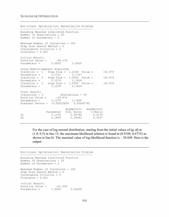
NONLINEAR OPTIMIZATION
105
Non-Linear Optimization: Maximization Problem---------------------------------------------Assuming Maximum Likelihood FunctionNumber of Observations = 20Number of Parameters = 2
Maximum Number of Iterations = 100Step Size Search Method = 0Convergence Criterion = 0Tolerance = 0.001
Initial Result:Function Value = -44.174Parameters = 3.0000 2.0000
Using Newton-Raphson AlgorithmIteration = 1 Step Size = 1.2100 Value = -43.974Parameters = 3.1323 2.1747Iteration = 2 Step Size = 1.0000 Value = -43.974Parameters = 3.1278 2.1809Iteration = 3 Step Size = 1.0000 Value = -43.974Parameters = 3.1278 2.1809
Final Result:Iterations = 3 Evaluations = 39Function Value = -43.974Parameters = 3.1278 2.1809Gradient Vector = -0.00010836 0.00040791
Asymptotic AsymptoticParameter Std. Error t-Ratio
X1 3.1278 0.48766 6.4139X2 2.1809 0.34483 6.3247
For the case of log-normal distribution, starting from the initial values of (µ, σ) at(1.0, 0.5) in line 15, the maximum likelihood solution is found at (0.9188, 0.6735) asshown in line16. The maximal value of log-likelihood function is – 38.849. Here is theoutput:
Non-Linear Optimization: Maximization Problem---------------------------------------------Assuming Maximum Likelihood FunctionNumber of Observations = 20Number of Parameters = 2
Maximum Number of Iterations = 100Step Size Search Method = 0Convergence Criterion = 0Tolerance = 0.001
Initial Result:Function Value = -41.299Parameters = 1.0000 0.50000

GAUSS PROGRAMMING FOR ECONOMETRICIANS AND FINANCIAL ANALYSTS
106
Using Newton-Raphson AlgorithmIteration = 1 Step Size = 1.9487 Value = -38.858Parameters = 0.89823 0.67385Iteration = 2 Step Size = 1.0000 Value = -38.849Parameters = 0.91884 0.67317Iteration = 3 Step Size = 1.0000 Value = -38.849Parameters = 0.91880 0.67349
Final Result:Iterations = 3 Evaluations = 44Function Value = -38.849Parameters = 0.91880 0.67349Gradient Vector = -0.0018227 0.027819
Asymptotic AsymptoticParameter Std. Error t-Ratio
X1 0.91880 0.15053 6.1039X2 0.67349 0.10637 6.3317
For the gamma distribution, the estimation of parameters λ and ρ is implemented inline 18 starting with the initial values 0.5 and 2.0 for λ and ρ, respectively (line 17).Maximum likelihood estimator of (λ, ρ) is obtained at (0.7707, 2.4106) where the log-likelihood function value is – 39.324. The output looks like this:
Non-Linear Optimization: Maximization Problem---------------------------------------------Assuming Maximum Likelihood FunctionNumber of Observations = 20Number of Parameters = 2
Maximum Number of Iterations = 100Step Size Search Method = 0Convergence Criterion = 0Tolerance = 0.001
Initial Result:Function Value = -40.628Parameters = 2.0000 0.50000
Using Newton-Raphson AlgorithmIteration = 1 Step Size = 1.4641 Value = -39.366Parameters = 2.2115 0.71252Iteration = 2 Step Size = 1.1000 Value = -39.324Parameters = 2.4112 0.77079Iteration = 3 Step Size = 1.0000 Value = -39.324Parameters = 2.4106 0.77070
Final Result:Iterations = 3 Evaluations = 42Function Value = -39.324Parameters = 2.4106 0.77070Gradient Vector = -0.0036550 0.0078771
Asymptotic AsymptoticParameter Std. Error t-Ratio
X1 2.4106 0.71610 3.3663

NONLINEAR OPTIMIZATION
107
X2 0.77070 0.25442 3.0293
To summarize the statistical characteristics of the random variable INCOME (dividedby 10) under consideration, we compute the estimated mean and variance of themaximum likelihood estimates of parameters from the normal, log-normal, andgamma probability distributions. We also compare the maximal values of the log-likelihood functions associated with these probability distributions. It is interesting tonote that the variable INCOME is more likely drawn from a log-normal or gammadistribution, as their log-likelihood function values are greater than that of the normaldistribution.
NormalDistribution
Log-NormalDistribution
GammaDistribution
Mean 3.1278 3.1443 3.1278Variance 4.7563 5.6745 4.0584Log-likelihood -43.974 -38.849 -39.324
Lesson 6.4: Mixture of Probability Distributions
It is possible that a random variable is drawn from a mixture of probabilitydistributions (two or more, same or different types of distributions). For simpleexploration, consider X is distributed with a mixture of two normal distributions:
f1(X,µ1,σ1) = 1
2πσ12 exp
(X-µ1)2
2σ12 ,
f2(X,µ2,σ2) = 1
2πσ22 exp
(X-µ2)2
2σ22 .
Then the likelihood function is
f(X,θ) = λ f1(X,µ1,σ1) + (1-λ) f2(X,µ2,σ2)
where λ is the probability that an observation is drawn from the first distributionf1(X,µ1,σ1), and 1-λ is the probability of that drawn from the second distribution. θ =(µ1,µ2,σ1,σ2,λ) is the unknown parameter vector must be estimated.
Continue from the previous example. Suppose each observation of the variableINCOME is drawn from one of two different normal distributions. There are fiveparameters, the first two are the mean and standard error of the first normaldistribution, while the second pair of parameters corresponds to the seconddistribution. The last parameter is the probability that the data is drawn from the first

GAUSS PROGRAMMING FOR ECONOMETRICIANS AND FINANCIAL ANALYSTS
108
distribution. Line 12 to 17 of Lesson 6.4 below defines the log-likelihood function forthe mixture of two normal distributions.
1234
5678910
11
121314151617
/*** Lesson 6.4: Mixture of Two Normal Distributions** See Greene (1999), Chapter 4*/use gpe2;output file=output6.4 reset;load data[21,2]=gpe\yed20.txt;x=data[2:21,1]/10; @ income data: scaling may help @
call reset;_nlopt=1;_method=5;_iter=100;_b=3,3,2,2,0.5;call estimate(&llf,x);
end;/*mixture of two normal distributionsmu1=b[1], mu2=b[2]se1=b[3], se2=b[4]prob.(drawn from the 1st distribution)=b[5]*/proc llf(x,b);
local pdf1,pdf2;pdf1=pdfn((x-b[1])/b[3])/b[3];pdf2=pdfn((x-b[2])/b[4])/b[4];retp(sumc(ln(b[5]*pdf1+(1-b[5])*pdf2)));
endp;
The problem is to maximize the log-likelihood function (_nlopt=1 in line 6) usingQHC algorithm (_method=5 in line 7) with the initial estimates of the parametersgiven in line 9. After 11 iterations, we obtain the following result (to save the space,we print only the first and last iterations):
Non-Linear Optimization: Maximization Problem---------------------------------------------Assuming Maximum Likelihood FunctionNumber of Observations = 20Number of Parameters = 5
Maximum Number of Iterations = 100Step Size Search Method = 0Convergence Criterion = 0Tolerance = 0.001
Initial Result:Function Value = -44.174Parameters = 3.0000 3.0000 2.0000 2.0000 0.50000
Using Quadratic Hill-Climbing AlgorithmIteration = 1 Step Size = 2.3579 Value = -43.996Parameters = 3.0542 3.0542 2.1325 2.1325 0.50000

NONLINEAR OPTIMIZATION
109
…Iteration = 11 Step Size = 1.0000 Value = -38.309Parameters = 2.0495 5.7942 0.81222 2.2139 0.71204
Final Result:Iterations = 11 Evaluations = 406Function Value = -38.309Parameters = 2.0495 5.7942 0.81222 2.2139 0.71204Gradient Vector = 1.1441e-005 0.00000 2.1870e-005 5.1351e-006 -4.7899e-005
Asymptotic AsymptoticParameter Std. Error t-Ratio
X1 2.0495 0.24421 8.3922X2 5.7942 1.4988 3.8659X3 0.81222 0.19424 4.1816X4 2.2139 0.90617 2.4431X5 0.71204 0.14456 4.9254
With the maximum log-likelihood function value of –38.309, the variable INCOMEwhich is drawn from the mixtures of two different normal probability distributions isequally convincing as that the variable is drawn from a single non-normal distribution(log-normal or gamma) as demonstrated in Lesson 6.3.
Statistical Regression ModelsEstimating probability distributions of a random variable is interesting, buteconometric modeling focuses on the statistical causal relationship between a group ofvariables. GPE package is designed specifically for statistical model estimation inmind. If the sample data, in addition to the parameters, is used to define the scalar-valued objective function, estimate assumes nonlinear least squares for aminimization problem and maximum likelihood for a maximization problem. Inaddition to reporting the optimization process and outcome, the estimated results areinterpreted according to these two types of statistical regression models. If yourproblem is neither a least squares nor a maximum likelihood, your own scrutiny intothe classical statistical interpretation of the model is necessary.
For a statistical model, the estimated variance-covariance matrix of the parametersmay be requested by setting a positive value to the input control variable _vcov.Typically, the estimated variance-covariance matrix is derived from the approximatedhessian (_vcov=1). A re-calculated exact hessian matrix is used instead if we set_vcov=2. Nevertheless, the estimated variance-covariance matrix may only bemeaningful in the contexts of nonlinear least squares and maximum likelihoodproblems.
As with the linear regression model, values of several output control variables areavailable after nonlinear least squares or maximum likelihood estimation:

GAUSS PROGRAMMING FOR ECONOMETRICIANS AND FINANCIAL ANALYSTS
110
• __b Estimated parameters or solution
• __vb Estimated variance of the parameters
• __e Estimated regression residuals.
• __rss Sum of squares function value at minimum
• __ll Log-likelihood function value at maximum
• __g Gradient vector of objective function at optimum
• __h Hessian matrix of objective function at optimum
Appendix A, GPE Control Variables, lists and explains the usage of these input andoutput control variables.
Lesson 6.5: Minimizing Sum-of-Squares Function
The following example is taken from Judge, et. al., (1988, Chapter 12, p.512).Consider a CES production function of a single output (Q) using two factors, labor (L)and capital (K), as follows:
ln(Q) = β1 + β4 ln (β2Lβ3 + (1-β2)K β3) + ε
Where ε is the error term and βs’are the unknown parameters. The data matrix X = (L,K, Q) is available in the text file judge.txt. The method of least squares estimation isto find the vector β = (β1,β2,β3,β4) so that the sum of squared errors S(β) = ε’ε isminimized.
Here is the program:
123
456789
/*** Lesson 6.5: Minimizing Sum-of-Squares Function** Estimating a CES Production Function** See Judge, et. al. (1988), Chapter 12*/use gpe2;output file=output6.5 reset;load x[30,3]=gpe\judge.txt;
call reset;_nlopt=0;_method=5;_iter=100;_tol=1.0e-5;_vcov=1;

NONLINEAR OPTIMIZATION
111
1011
12
1314151617181920
_b=1.0,0.5,-1.0,-1.0;call estimate(&cessse,x);
end;
/* Objective Function */proc cessse(data,b); @ sum-of-squares function @
local l,k,q,e;l=data[.,1];k=data[.,2];q=data[.,3];e=ln(q)-b[1]-b[4]*ln(b[2]*l^b[3]+(1-b[2])*k^b[3]);retp(sumc(e^2));
endp;
The objective function cessse, sum-of-squared errors, is defined as a procedure inlines 13 through 20. It is evident that both data matrix data and parameter vector bare used to specify the functional form. The address of function &cessse is used incalling estimate in line 11, where x is the data matrix (see also line 3). Line 5indicates that the problem is to minimize the objective function cessse, and line 6requests the quadratic hill-climbing (QHC, i.e., _method=5) optimization method.In line 8, the convergence of function value and solutions are checked relative to asmaller tolerance level of 0.00001. The vector of initial parameter values _b is givenin line 10, which is rather a random guess. Finally, at the end of optimization, thevariance-covariance matrix of estimated parameters will be computed because_vcov=1 as shown in line 9.
We keep the definition of objective function cessse outside (beyond the endstatement) of the main program in the bottom. There is no strict rule dictating whereto place the functions you define. Putting the function or procedure outside of themain program makes the function accessible to other procedures you write for otherpurposes.
Final solution is found after 36 iterations. To save the space, we report only the finalresult of the iterations. The output file output6.5 keeps the details of all theiterations for reference.
In your program, setting _print=0 will suppress the printing of iteration outputs tofile and screen.
Non-Linear Optimization: Minimization Problem---------------------------------------------Assuming Nonlinear Least Squares FunctionNumber of Observations = 30Number of Parameters = 4
Maximum Number of Iterations = 100Step Size Search Method = 0Convergence Criterion = 0

GAUSS PROGRAMMING FOR ECONOMETRICIANS AND FINANCIAL ANALYSTS
112
Tolerance = 1e-005
Initial Result:Function Value = 37.097Parameters = 1.0000 0.50000 -1.0000 -1.0000
Using Quadratic Hill-Climbing Algorithm
Final Result:Iterations = 36 Evaluations = 1012Function Value = 1.7611Parameters = 0.12449 0.33668 -3.0109 -0.33631Gradient Vector = 2.6755e-006 4.6166e-007 2.5664e-006 1.7166e-006Hessian Matrix =
60.000 -5.7563 35.531 295.65-5.7563 19.377 -3.4569 -23.59535.531 -3.4569 35.461 298.10295.65 -23.595 298.10 2509.4
AsymptoticParameter Std. Error t-Ratio
X1 0.12449 0.074644 1.6678X2 0.33668 0.10809 3.1147X3 -3.0109 2.2904 -1.3145X4 -0.33631 0.26823 -1.2538
Asymptotic Variance-Covariance MatrixX1 0.0055717X2 -0.0013729 0.011684X3 -0.065566 0.16893 5.2462X4 0.0071194 -0.019797 -0.61389 0.071948
X1 X2 X3 X4
Both gradient and hessian of the solution confirm that the solution indeed minimizesthe sum-of-squares objective function at the value 1.761. The estimated model ispresented as follows:
ln(Q) = 0.125 - 0.336 ln (0.337 L –3.01 + 0.663 K –3.01)s.e. (0.075) (0.268) (0.108) (2.29)
Lesson 6.6: Maximizing Log-Likelihood Function
The same problem can be estimated by maximizing the likelihood objective function.Assuming the model error ε follows a normal probability distribution with zero meanand constant variance σ2, the log output ln(Q) is normally distributed with thefollowing distribution function:
N2πσ2 exp
ε(X,β)'ε(X,β)
2σ2

NONLINEAR OPTIMIZATION
113
Where N is the sample size, and ε(X, β) = ln(Q) - β1 - β4 ln (β2L β3 + (1-β2)K β3). Thecorresponding log-likelihood function of the unknown parameters θ = (β,σ) is writtenas
ll(θ) = -N/2 ln(2π) – N/2 ln(σ2) – ½
ε(X,β)'
σ
ε(X,β)
σ
The following program is basically the same as the one for minimizing sum-of-squaresfunction. By editing from the previous Lesson 6.5, change the objective function inthe call estimate to cesll (line 11) and set the variable _nlopt=1 (line 5). InLesson 6.6 below, the objective log-likelihood function cesll is defined from line13 to 21. In addition to β, the standard error of the model σ must be estimatedsimultaneously. Line 10 sets out the initial values of θ = (β,σ).
123
4567891011
12
131415161718192021
/*** Lesson 6.6: Maximizing Log-Likelihood Function** Estimating a CES Production Function** See Judge, et. al. (1988), Chapter 12*/use gpe2;output file=output6.6 reset;load x[30,3]=gpe\judge.txt;
call reset;_nlopt=1;_method=5;_iter=100;_tol=1.0e-5;_vcov=1;_b=1.0,0.5,-1.0,-1.0,1.0;call estimate(&cesll,x);
end;
/* Objective Function */proc cesll(data,b); @ log-likelihood function @
local l,k,q,e,n;l=data[.,1];k=data[.,2];q=data[.,3];e=ln(q)-b[1]-b[4]*ln(b[2]*l^b[3]+(1-b[2])*k^b[3]);n=rows(e);retp(-0.5*n*(ln(2*pi)+ln(b[5]^2))-0.5*sumc((e./b[5])^2));
endp;
Solving the maximization problem of a classical log-likelihood function, the standarderror parameter σ is shown to be dependent on β. That is, if β is known, σ2 is solvedas:
σ2(β) = ε(X,β)’ε(X,β)/Ν

GAUSS PROGRAMMING FOR ECONOMETRICIANS AND FINANCIAL ANALYSTS
114
Therefore, the same maximum log-likelihood may be expressed with theconcentrated log-likelihood function instead:
ll*(β) = -N/2 (1+ ln(2π) – ln(N)) –N/2 ln(ε(X,β)’ε(X,β))
The advantage of using the concentrated log-likelihood function is that there is oneless parameter (that is, σ) to estimate directly.
Running the program Lesson 6.6, we obtain the following result (again, the details ofinterim iterations can be found in the output file output6.6):
Non-Linear Optimization: Maximization Problem---------------------------------------------Assuming Maximum Likelihood FunctionNumber of Observations = 30Number of Parameters = 5
Maximum Number of Iterations = 100Step Size Search Method = 0Convergence Criterion = 0Tolerance = 1e-005
Initial Result:Function Value = -46.117Parameters = 1.0000 0.50000 -1.0000 -1.0000 1.0000
Using Quadratic Hill-Climbing Algorithm
Final Result:Iterations = 41 Evaluations = 1419Function Value = -0.039074Parameters = 0.12449 0.33667 -3.0109 -0.33630 0.24229Gradient Vector = 8.5614e-006 1.0552e-006 -8.2596e-007 7.3948e-006 -3.6658e-006Hessian Matrix =
-511.05 49.030 -302.63 -2518.3 0.06343249.030 -165.04 29.444 200.98 0.020503-302.63 29.444 -302.02 -2539.1 -0.037482-2518.3 200.98 -2539.1 -21375. -2.65560.063432 0.020503 -0.037482 -2.6556 -1021.5
AsymptoticParameter Std. Error t-Ratio
X1 0.12449 0.074646 1.6677X2 0.33667 0.10811 3.1142X3 -3.0109 2.2911 -1.3142X4 -0.33630 0.26830 -1.2535X5 0.24229 0.031295 7.7421
Asymptotic Variance-Covariance MatrixX1 0.0055721X2 -0.0013740 0.011687X3 -0.065602 0.16904 5.2493X4 0.0071233 -0.019807 -0.61423 0.071984X5 -1.5793E-005 4.5442E-005 0.0014036 -0.00016456 0.00097936

NONLINEAR OPTIMIZATION
115
X1 X2 X3 X4 X5
It is no surprise that the solution is identical to the one obtained from minimizing thesum-of-squares function in Lesson 6.5. In addition, the estimated standard error of thenormal distribution is found to be 0.2423, or σ2 = 0.0587. This also confirms theminimal sum-of-squares S(β) = Nσ2 = 1.761.
Minimizing sum-of-squares and maximizing log-likelihood are popular techniques foreconometric model estimation. In the next chapter on nonlinear regression models, forthe convenience of classical econometric analysis, it is only the functional form ofmodel error ε(X,β) that we will need to specify. The objective of either minimizing asum-of-squares or maximizing a log-likelihood is readily available once the specificerror structure is given. Nevertheless, as we have leraned from this chapter, being ableto work on the scalar-valued objective function directly is useful when dealing withdifficult optimization problems.


VIINonlinear Regression Models
Many economic and econometric problems can be formulated as optimization(minimization or maximization) problems. In econometrics, sum of squaresminimization and log-likelihood maximization are standard in empirical modelestimation. In the previous chapter, we defined a scalar-valued objective function tominimize (maximize) and interpreted the parameter estimates in accordance with theclassical least squares (maximum likelihood) model. This approach is flexible enoughto encompass many different econometric models. In many situations, however, itbecomes troublesome to write out the objective function in detail. It is more desirableto present only the functional form which defines the model directly, such as
F(Z,β) = ε
Where Z is the data matrix, β is the parameter vector, and ε is the error term. Both Zand β are used to define the functional form of the model (that is, the error structure).The data matrix Z can be further decomposed as Z = [Y, X] where Y consists ofendogenous (dependent) variables and X is a list of predetermined (independent)variables. For a classical single regression equation, Y = f(X,β) + ε or ε = Y - f(X,β).The special case of linear model is simply ε = Y - Xβ.
Nonlinear Least SquaresThe functional form F(Z,β) = ε is of interest in econometric modeling. Consider thesum-of-squares objective function:
S(β) = ε’ε
A nonlinear least squares estimator b of β is computed from the first-order conditionfor minimization (or the zero gradient condition) as follows:
∂S(b)/∂β = 2ε’(∂ε/∂β) = 0
In addition, the hessian matrix of second derivatives evaluated at b:
∂2S(b)∂β∂β' = 2 [(∂ε/∂β)’(∂ε/∂β) + ∑i=1,2,…,N εi
∂2εi
∂β∂β' ]

GAUSS PROGRAMMING FOR ECONOMETRICIANS AND FINANCIAL ANALYSTS
118
must be positive definite to guarantee the minimum solution. The estimated variance-covariance matrix of the parameters is derived from the expected values of thehessian:
Var(b) = s2 [½ E
∂2S(b)
∂β∂β' ]-1 = s2 [(∂ε/∂β)’(∂ε/∂β)]−1
Where s2 = e’e/N is the estimated regression variance σ2, e = F(Z,b) is the estimatederrors, and N is the sample size used for estimation. It becomes clear that only theinformation concerning the functional form F(Z,β), and its first and second derivativesare needed to carry out the nonlinear least squares estimation of b, e, s2, and Var(b).
It is straightforward to generalize the technique of nonlinear least squares to considerweighted model errors. Denote the weighting scheme w = w(Z,β). The variable w is ascalar or a vector, which in turn may depend on part or all of the data and parameters.Define the weighted error terms as ε* = w ε. Then the model is estimated byminimizing the sum of squared weighted errors: S*(β) = ε*’ε*.
Lesson 7.1: CES Production Function
Let’s return to the example of Lesson 6.5 estimating a nonlinear CES productionfunction. Instead of defining and minimizing the sum-of-squares objective function,this example demonstrates the use of the error or residual function for modelestimation. A residual function is usually more intuitive and easier to write than asum-of-squares function. Since the computation of least squares relies on the residualsand their derivatives, the advantage of increased numerical precision is another reasonof working with the residuals directly.
The setup of input control variables is the same as in Lesson 6.5. The difference is theuse of the residual function (instead of sum-of-squares objective function) in callingthe estimate procedure (line 12). The residual function ces is defined in the blockfrom line 14 to line 20.
123
4
567
/*** Lesson 7.1: CES Production Function Revisited** Judge, et. al. (1988), Chapter 12*/use gpe2;output file=gpe\output7.1 reset;load x[30,3]=gpe\judge.txt;
call reset;
_nlopt=0; @ NLSQ: SSE minimization @_method=5; @ optimization method @_iter=100;

NONLINEAR REGRESSION MODELS
119
8910
11
12
13
14151617181920
_tol=1.0e-5;_conv=1;_vcov=1;
_b=1.0,0.5,-1.0,-1.0;
call estimate(&ces,x);
end;
proc ces(data,b); @ residual function @local l,k,q;l=data[.,1];k=data[.,2];q=data[.,3];retp(ln(q)-b[1]-b[4]*ln(b[2]*l^b[3]+(1-b[2])*k^b[3]));
endp;
The regression output duplicates that of Lesson 6.5, and it is avaialable in the outputfile output7.1.
Maximum Likelihood EstimationTo explore the idea of maximum likelihood estimation in the econometric context, weassume a classical normal probability distribution for the independent model error ε =F(Z,β). That is, ε is normally independently distributed with zero mean and constantvariance σ2. Then the probability density function of Y (recall that Z = [Y, X]) iswritten as:
12πσ2 exp
-
F(Z,β)2
2σ2 |J(Z,β)|
Where J(Z,β) = ∂ε/∂Y is the Jacobian of the transformation from ε to Y. Samplingover N independent observations, the log-likelihood function of the unknownparameter vector θ = (β,σ) is:
ll(θ) = -N/2 ln(2π) – N/2 ln(σ2) – ½
F(Z,β)'
σ
F(Z,β)
σ + ∑i=1,2,…,N ln|J(Zi,β)|
The technique of maximum likelihood estimation is to find the θ that maximizes thelog-likelihood function ll(θ). Usually the computation is performed by substituting outthe variance estimate σ2 = ε’ε/N = F(Z,β)’F(Z,β)/N. Then the following concentratedlog-likelihood function is maximized with respect to the parameter vector β:
ll*(β) = -N/2 [1 + ln(2π) – ln(N)] – N/2 ln[F(Z,β)’F(Z,β)] + ∑i=1,2,…,N ln|J(Zi,β)|

GAUSS PROGRAMMING FOR ECONOMETRICIANS AND FINANCIAL ANALYSTS
120
Define ε* = ε/[(∏i=1,2,…,N|Ji|)1/N] or equivalently F*(Z,β) = F(Z,β)/[(∏i=1,2,…,N|Ji|)1/N],where Ji = J(Zi,β). Then the last two terms of the above concentrated log-likelihoodfunction can be combined and the function is re-written as:
ll*(β) = -N/2 [1 + ln(2π) – ln(N)] – N/2 ln[F*(Z,β)’F*(Z,β)]
Where F*(Z,β) = ε* is the weighted error, with the weight being the inverse of thegeometric mean of Jacobians (that is, 1/[(∏i=1,2,…,N|Ji|)1/N]). Therefore, maximizing theconcentrated log-likelihood function ll*(β) is equivalent to minimizing thecorresponding sum of squared weighted errors S*(β) = ε*’ε*.
The maximum likelihood estimator b of β is obtained from solving from the first-order condition (recall that S* = ε*’ε* and ε* = F*(Z,β)):
∂ll*(b)/∂β= -½ (N/S*)(∂S*/∂β) = -(N/S*)[ε*’(∂ε*/∂β)] = 0
We must also check that the hessian matrix is negative definite (the second-ordercondition for maximization) at b:
∂2ll*(b)∂β∂β' = -½ (N/S*)[(1/S*)(∂S*/∂β)’(∂S*/∂β) -
∂2S*∂β∂β' ]
Since ∂S*/∂β = 0, at the maximum, the corresponding negative definite hessian matrixis simply:
∂2ll*(b)∂β∂β' = - (N/S*)[½
∂2S*
∂β∂β' ]
= - (N/S*)[(∂ε*/∂β)’(∂ε*/∂β) + ∑i=1,2,…,N ε i*’
∂2εi*
∂β∂β' ]
Thus the estimated variance-covariance matrix of maximum likelihood estimator b,defined as the inverse of negative expected hessian, is:
Var(b) = [-E
∂2ll*(b)
∂β∂β' ]-1 = s2* [(∂ε*/∂β)’(∂ε*/∂β)]-1
Where s2* = e*’e*/N, and e* = F*(Z,b) = F(Z,b)/[(∏i=1,2,…,N|Ji|)1/N],. Therefore, if theobjective is to maximize the log-likelihood function under the assumption of normallyindependently distributed model error, then we need only to be concerned with theresidual function ε = F(Z,β) and its associated Jacobian transformations J(Z,β).

NONLINEAR REGRESSION MODELS
121
There is a new GPE input variable _jacob of GPE we have not yet introduced,which controls the use of Jacobians in deriving the objective function (log-likelihoodor sum-of-squares) from the residuals. Notice that a Jacobian transformation isnothing but a function of data and parameters. If you define a Jacobian function ofyour own, then _jacob should be set to the location (address) of the function. Anexample of Jacobian function is given later in Lesson 7.2 on Box-Cox variabletransformation. If you do not wish to write out the Jacobian analytically, you may set
_jacob = 1;
Then the numerical Jacobian is computed for each sample observation, which isusually a time consuming process. In case of requesting numerical Jacobians, the firstcolumn of the data matrix used to define the residuals must be the dependent variableY (recall that J(Z,β) = ∂ε/∂Y and Z = [Y,X]).
Here, based on Lesson 7.1 above, we insert the following statement before calling theestimate procedure in line 12:
_jacob = 0;
Although it is not necessary (_jacob=0 by default), _jacob=0 is used here tomake sure that you understand the implication of Jacobian terms in the log-likelihoodfunction. As a matter of fact, for the classical model of the CES production function,there is no need to consider the vanishing Jacobian terms in the log-likelihoodfunction.
Lesson 7.1 may be modified to carry out maximum likelihood estimation instead.Change the type of problem from minimization to maximization in line 5:
_nlopt = 1;
It is no surprise that the empirical results are identical for both techniques of nonlinearleast squares and maximum likelihood.
If you ask for the numerical Jacobians to be computed in this example:
_jacob = 1;
You must be sure that the first column of the data matrix data used to define theresidual function ces(data,b) corresponds to the dependent variable of themodel, ln(Q) in this case. As it was presented in Lesson 7.1, this rule is not followed.You may want to correct the data matrix and rewrite the procedure ces(data,b)so that you can use the numerical Jacobians which are all ones. The estimation resultshould not be affected.

GAUSS PROGRAMMING FOR ECONOMETRICIANS AND FINANCIAL ANALYSTS
122
Box-Cox Variable Transformation
A nonlinear regression equation may involve non-linearity in both parameters andvariables. The Box-Cox variable transformation is a classic example of a nonlinearmodel in econometrics. The so-called Box-Cox transformation of a data variable X isdefined by
X(λ) = (Xλ-1)/λ
Although the range of λ can cover the whole set of real numbers, -2 ≤ λ ≤ 2 is the areaof interests in many econometric applications. λ = 2 corresponds to a quadratictransformation, while λ = ½ is a square-root transformation. A linear modelcorresponds to λ =1, and the logarithmic transformation is the limiting case where λapproaches 0 (by L’Hôspital’s rule, limλ−>0 (Xλ-1)/λ = ln(X)).
The value of power transformation parameter λ may not have to be the same for eachvariable in the model. In particular, the dependent variable and independent variablesas a group may need different Box-Cox transformations. Let β = (α,λ,θ) be the vectorof unknown parameters for a regression model:
ε = F(Z,β) = F(Y,X,β) = Y(θ) – X(λ)α
Or, equivalently,
Y(θ) = X(λ)α + ε
To estimate the parameters, we assume the error ε is normally independentlydistributed with zero mean and constant variance σ2. The log-likelihood function ofthe random variable Y is
ll(β) = -N/2 [ln(2π) + ln(σ2)] - ½ F(Z,β)’F(Z,β)/σ2 + (θ-1)∑i=1,2,…,N ln(|Yi|)
Z = [Y,X], β = (α,λ,θ), and for each data observation i, the Jacobian term of thefunction is derived as J(Yi,θ) = ∂εi/∂Yi = Yi
(θ-1). By substituting out the variance σ2 =ε’ε/N, the concentrated log-likelihood function is
ll*(β) = -N/2 [1+ln(2π)-ln(N)] – N/2 ln(F(Z,β)’F(Z,β)) + (θ-1)∑i=1,2,…,N ln(|Yi|)= -N/2 [1+ln(2π)-ln(N)] – N/2 ln(F*(Z,β)’F*(Z,β))
Where F*(Z,β) = ε* = ε/[(∏i=1,2,…,N |Yi|)(θ−1)/N]. Given the values of Box-Coxtransformation parameters θ and λ, a wide range of model specifications are possible.Of course, θ and λ must be estimated jointly with α. An efficient estimator of theparameter vector β = (α,λ,θ) is obtained by maximizing the above concentrated log-

NONLINEAR REGRESSION MODELS
123
likelihood function. It is equivalent to minimizing the sum of squared weighted errorsS(β) = ε*’ε*, where ε* = w ε and w = w(Y,θ) = 1/[(∏i=1,2,…,N |Yi|)(θ−1)/N].
Lesson 7.2: Box-Cox Variable Transformation
The following example of U. S. money demand equation is taken from Greene (1999,Chapter 10):
M(θ) = α0 + α1 R(λ) + α2 Y(λ) + ε
As described in Greene’s Example 10.9, M is the real money stock M2, R is thediscount interest rate, and Y is real GNP. money.txt is the data text file consisting ofthese variables. Several variations of the Box-Cox transformation may be estimatedand tested for selecting the most appropriate functional form of the money demandequation:
1. θ −> 0 ln(M) = α0 + α1 R(λ) + α2 Y(λ) + ε2. θ = 1 M = α0 + α1 R(λ) + α2 Y(λ) + ε3. λ −> 0 M(θ) = α0 + α1 ln(R) + α2 ln(Y) + ε4. λ = 1 M(θ) = α0 + α1 R + α2 Y + ε5. θ = λ M(λ) = α0 + α1 R(λ) + α2 Y(λ) + ε6. θ, λ −> 0 ln(M) = α0 + α1 ln(R) + α2 ln(Y) + ε7. θ, λ = 1 M = α0 + α1 R + α2 Y + ε
The following program considers a general case of Box-Cox variable transformation.In addition to the regression parameters α, there are two power transformationparameters: θ for the left-hand-side variable and λ for the right-hand-side. All theseparameters (α,λ,θ) are estimated jointly. For model estimation, it is typical to scale thevariables so that their power transformations do not under- or over-flow in arithmeticcomputation. This will make the interpretation of the estimated parameters moredifficult. The sensible approach is to convert the estimated values of the parameters tounit-free measurements of elasticity. Therefore, for the general model, the estimatedelasticity of the interest rate is
∂ln(M)∂ln(R) =
RM
∂M∂R = α1
Rλ
Mθ
Similarly, the elasticity of GNP is ∂ln(M)∂ln(Y) = α2
Yλ
Mθ . The elasticity at the means (of
data variables) should be reported for model interpretation.
/*** Lesson 7.2: Box-Cox Transformation

GAUSS PROGRAMMING FOR ECONOMETRICIANS AND FINANCIAL ANALYSTS
124
123
4
5678910
1112
131415
1617181920
2122
232425262728
** U. S. Money Demand Equation** Greene (1999), Chapter 10*/use gpe2;output file=gpe\output7.2 reset;load x[21,4]=gpe\money.txt;@ scale and re-arrange data: m,r,y @x=(x[2:21,3]/1000)~(x[2:21,2])~(x[2:21,4]/1000);
call reset;_method=0;_iter=200;_step=1;_conv=1;_jacob=&jf;
@ starting linear model @b=x[.,1]/(ones(rows(x),1)~x[.,2:3]);_b=b|1.0|1.0;/*@ starting log model @b=ln(x[.,1])/(ones(rows(x),1)~ln(x[.,2:3]));_b=b|-0.01|0.01;*/_nlopt=1; @ MAXLIK @call estimate(&rf,x);end;
proc jf(data,b); @ jacobian @local k;k=rows(b); @ the last parameter @retp(data[.,1]^(b[k]-1));
endp;
proc rf(data,b); @ residual: general model @local r,m,y,e;@ box-cox transformation @m=(data[.,1]^b[5]-1)/b[5];r=(data[.,2]^b[4]-1)/b[4];y=(data[.,3]^b[4]-1)/b[4];e=m-b[1]-b[2]*r-b[3]*y;retp(e);
endp;
The residual function for the general model rf is defined in lines 21 through 28.Notice that the residual function is written in such a way that the first column of thedata matrix is the dependent variable. The procedure jf, given in the block from line16 to line 20, defines the Jacobian terms for the likelihood function. Recall that theJacobian term is just Yθ-1 for the Box-Cox model, where Y is the left-hand-sidedependent variable. As we have mentioned earlier in Lesson 7.1, the GPE inputvariable _jacob controls the use of Jacobian transformation in defining the log-likelihood and sum-of-squares functions. In the case of Box-Cox variabletransformation, the residuals are weighted with the inverse of geometric mean ofJacobians: 1/[(∏i=1,2,…,N |Ji|)1/N] and Ji = Yi
θ-1. When _jacob=0, the Jacobians are notused (vanishing log-Jacobians is assumed). When _jacob=1, the numerical

NONLINEAR REGRESSION MODELS
125
Jacobians are computed from the residual function with the assumption that the firstcolumn of the data matrix is the dependent variable under consideration. When_jacob is set to the location (address) of a procedure defining the analyticalJacobians, the result of the procedure called is used. Here, in line 10:
_jacob = &jf;
The input control variable _jacob is assigned the result of the procedurejf(data,b). Therefore, the analytical Jacobian transformation is used for log-likelihood maximization and sum-of-squares (weighted) minimization. By definingand applying the Jacobian transformation, as we have done here, guarantee that ourparameters will be efficiently estimated.
Although numerical Jacobians may be requested instead, by setting _jacob=1 inline 10, we recommend against using it. The numerical approximation of Jacobiantransformation is typically slower and results in less accurate parameter estimatesthan explicitly defining the analytical formula. As in the case of defining the residualfunction, the Jacobian function is problem-dependent and it involves differentiationof the residual function with respect to the dependent variable. For optimization,another round of differentiation of the residual and Jacobian functions is needed.Rounding errors due to excess numerical approximation may be too severe to yieldan accurate solution.
Two sets of starting values of the parameters may be tried: one from the linear modelestimates and the other from log model. In the program, we start with the linear modelestimates (line 11 and 12). The alternative is to start with the log model estimates asgiven in the comment block immediately below line 12. Just to make sure that youachieve the same solution starting from several different initial values of theparameters. Run the program Lesson7.2, and check the following result:
Maximum Likelihood Estimation-----------------------------Number of Observations = 20Number of Parameters = 5
Maximum Number of Iterations = 200Step Size Search Method = 1Convergence Criterion = 1Tolerance = 0.001
Initial Result:Sum of Squares = 7.0963Log Likelihood = -18.017Parameters = -3.1694 -0.014921 1.5881 1.0000 1.0000
Using Berndt-Hall-Hall-Hausman (BHHH) Algorithm
Final Result:Iterations = 165 Evaluations = 29500

GAUSS PROGRAMMING FOR ECONOMETRICIANS AND FINANCIAL ANALYSTS
126
Sum of Squares = 0.11766Log Likelihood = 22.978Gradient of Log Likelihood = -8.2374e-005 -3.0382e-005 -2.8533e-005 -0.00032734 -6.0704e-005
AsymptoticParameter Std. Error t-Ratio
X1 -14.503 12.127 -1.1959X2 -14.067 50.134 -0.28058X3 56.399 106.75 0.52831X4 -2.6723 1.8562 -1.4396X5 -0.96447 0.54949 -1.7552
Model interpretation of Box-Cox variable transformation is more difficult than that oflinear models. However, the elasticity at the mean of each variable is computed andinterpreted as below:
M (-0.96) = -14.5 - 14.07 R (−2.67) + 56.4 Y (-2.67)
s.e. (0.55) (12.13) (50.13) (1.86) (106.75) (1.86)Elasticity - 0.087 4.252
The same model may be estimated with the technique of weighted least squares. Aslong as the Jacobian is used, the sum-of-squares function is derived from theresiduals, weighted by the inverse of the geometric mean of the Jacobians. Justreplace line 13 with:
_nlopt=0;
This should produce the same result as that from the maximum likelihood estimation.However, if we attempt to minimize the sum of squared un-weighted residuals, thenthe estimation result will not be efficient. It can even be biased. Check it out bydeleting line 10 or changing it to:
_jacob=0;
The program of Lesson 7.2 is readily modifiable to accommodate all of the specialcases of Box-Cox transformations. For example, for the case θ = λ, let’s define theresidual function rf1 as follows:
proc rf1(data,b);local r,m,y,e;@ box-cox transformation @m=(data[.,1]^b[4]-1)/b[4];r=(data[.,2]^b[4]-1)/b[4];y=(data[.,3]^b[4]-1)/b[4];e=m-b[1]-b[2]*r-b[3]*y;retp(e);
endp;

NONLINEAR REGRESSION MODELS
127
To run this special case, modify the starting values for the parameters (note that thenumber of parameters is changed as well) and call estimate with &rf1. That is,the lines from 12 to 14 should read like this:
_b=b|1.0;_nlopt=1;call estimate(&rf1,x);
Other cases such as linear or log transformation on one side of the equation can beestimated as long as the respective residual function is defined and used correctly.You may have to experiment with different combinations of optimization options andstarting values for finding all the solutions. Also, the last two cases of linear and logmodels may be more conveniently estimated with linear least squares. We leave theremainder of these special cases to you as exercises.
From Lesson 7.2, we have estimated the general Box-Cox transformation model,together with many special cases. It is useful to tabulate and compare the estimationresults of all these models. Based on the sample data series in money.txt, what is themost appropriate functional form for the U. S. money demand equation? To answerthis question, some knowledge of statistical inference will be necessary.
Statistical Inference in Nonlinear ModelsA fundamental assumption of statistical inference is the normality of the model error:ε = F(Z,β). In particular, ε is assumed to be identically independently normallydistributed with zero mean and constant variance σ2, or ε ~ nii(0,σ2). Thus theestimated least squares or maximum likelihood parameters b of β is normallydistributed with the mean as β and the estimated variance-covariance matrix as:
Var(b) = [-E(∂2ll(b)/∂β'∂β)]-1
= s2 [½ E(∂2S(b)/∂β'∂β)]-1
Where s2 = S(b)/N is the estimated asymptotic variance of the model. Note that S(b) =e’e and e = F(Z,b).
In many situations, it is of interest to test the validity of a set of J non-samplerestrictions of the parameters, linear or nonlinear (continuous and differentiable),expressed as the following vector-valued equation:
c(β) = 0.
If there are J active parameter restrictions, let the restricted parameter estimator andits variance-covariance matrix be b* and Var(b*), respectively. For example, thesimplest case of a linear restriction c(β) = β - β0 (possibly a vector) confines the

GAUSS PROGRAMMING FOR ECONOMETRICIANS AND FINANCIAL ANALYSTS
128
parameter vector β to be near β0. The following three tests are useful for inferenceabout the model restrictions.
Wald Test
Without estimating the constrained model, the unconstrained parameter estimator b isexpected to satisfy the constraint equation closely, if the hypothesis is true. That is,c(b) = 0. The Wald test statistic:
W = c(b)'[Var(c(b)]-1c(b)
has a Chi-square distribution with J degrees of freedom (remember that J is thenumber of restrictions). With the first-order linear approximation of the constraintfunction c(β) at b,
W = c(b)' (∂c(b)/∂β) [Var(b)] (∂c(b)/∂β)'-1 c(b)
Note that this test statistic does not require the computation of the constrainedparameters.
Lagrangian Multiplier (LM) Test
Given the J-element constraint equation c(β) = 0, let b* denote the maximumlikelihood estimator of the parameter vector β with the constraint in place. TheLagrangian multiplier test is based on the score vector ∂ll(b*)/∂β of the originalparameterization of the log-likelihood function. If the constraints hold, then ∂ll(b*)/∂βshould be close to ∂ll(b)/∂β for the unconstrained parameter estimator b, which is ofcourse zero. The Lagrangian multiplier test statistic is written as:
LM = (∂ll(b*)/∂β) [Var(b*)] (∂ll(b*)/∂β)'
The estimated variance-covariance matrix of the constrained estimator b* is computedas follows:
Var(b*) = H-1 [I - G'(G H-1G')-1H-1]
where H = [-∂ll(b*)2/∂β'∂β] and G = [∂c(b*)/∂β]. In practice, LM test statistic is easilyapproximated with the following formula:
LM = [e*'(∂e*/∂β)] [(∂e*/∂β)'(∂e*/∂β)]-1 [e*'(∂e*/∂β)]'/(e*'e*/N)
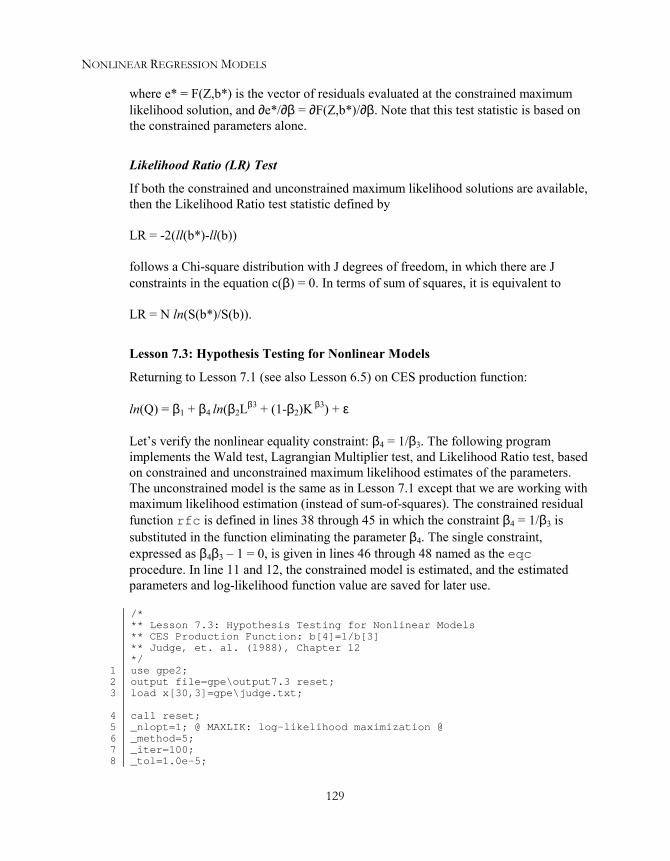
NONLINEAR REGRESSION MODELS
129
where e* = F(Z,b*) is the vector of residuals evaluated at the constrained maximumlikelihood solution, and ∂e*/∂β = ∂F(Z,b*)/∂β. Note that this test statistic is based onthe constrained parameters alone.
Likelihood Ratio (LR) Test
If both the constrained and unconstrained maximum likelihood solutions are available,then the Likelihood Ratio test statistic defined by
LR = -2(ll(b*)-ll(b))
follows a Chi-square distribution with J degrees of freedom, in which there are Jconstraints in the equation c(β) = 0. In terms of sum of squares, it is equivalent to
LR = N ln(S(b*)/S(b)).
Lesson 7.3: Hypothesis Testing for Nonlinear Models
Returning to Lesson 7.1 (see also Lesson 6.5) on CES production function:
ln(Q) = β1 + β4 ln(β2Lβ3 + (1-β2)K β3) + ε
Let’s verify the nonlinear equality constraint: β4 = 1/β3. The following programimplements the Wald test, Lagrangian Multiplier test, and Likelihood Ratio test, basedon constrained and unconstrained maximum likelihood estimates of the parameters.The unconstrained model is the same as in Lesson 7.1 except that we are working withmaximum likelihood estimation (instead of sum-of-squares). The constrained residualfunction rfc is defined in lines 38 through 45 in which the constraint β4 = 1/β3 issubstituted in the function eliminating the parameter β4. The single constraint,expressed as β4β3 – 1 = 0, is given in lines 46 through 48 named as the eqcprocedure. In line 11 and 12, the constrained model is estimated, and the estimatedparameters and log-likelihood function value are saved for later use.
123
45678
/*** Lesson 7.3: Hypothesis Testing for Nonlinear Models** CES Production Function: b[4]=1/b[3]** Judge, et. al. (1988), Chapter 12*/use gpe2;output file=gpe\output7.3 reset;load x[30,3]=gpe\judge.txt;
call reset;_nlopt=1; @ MAXLIK: log-likelihood maximization @_method=5;_iter=100;_tol=1.0e-5;

GAUSS PROGRAMMING FOR ECONOMETRICIANS AND FINANCIAL ANALYSTS
130
910
1112131415161718
192021222324
25
26272829
3031323334353637
3839404142434445
464748
_conv=1;_jacob=0; @ vanishing log-jacobians @
/* Lagrangian Multiplier Test */@ based on constrained estimation @_b=1.0,0.5,-1.0;call estimate(&rfc,x);b1=__b|(1/__b[3]); @ original parametrization, b[4]=1/b[3] @ll1=__ll; @ log-likelihood @e=rf(x,b1); @ estimated errors @s2=meanc(e^2); @ estimated error variance @g=gradp2(&rf,x,b1); @ gradient of error function @lm=(e'g)*invpd(g'g)*(g'e)/s2;
/* Wald Test */@ based on unconstrained estimation @_b=1.0,0.25,-1.0,-1.0;call estimate(&rf,x);b2=__b; @ estimated parameters @vb2=__vb; @ estimated var-cov. of parameters @ll2=__ll; @ log-likelihood @w=eqc(b2)'*invpd(gradp(&eqc,b2)*vb2*gradp(&eqc,b2)')*eqc(b2);
/* Likelihood Ratio Test */lr=-2*(ll1-ll2);
print "Wald Test = " w;print "Lagrangian Multiplier Test = " lm;print "Likelihood Ratio Test = " lr;end;
proc rf(data,b); @ unconstrained residual function @local l,k,q,e;l=data[.,1];k=data[.,2];q=data[.,3];e=ln(q)-b[1]-b[4]*ln(b[2]*l^b[3]+(1-b[2])*k^b[3]);retp(e);
endp;
proc rfc(data,b); @ constrained residual function @local l,k,q,n,e;l=data[.,1];k=data[.,2];q=data[.,3];e=ln(q)-b[1]-(1/b[3])*ln(b[2]*l^b[3]+(1-b[2])*k^b[3]);retp(e);
endp;
proc eqc(b); @ constraint function @retp(b[3]*b[4]-1);
endp;
Here is the estimation result of the constrained model as of line 12 (see alsooutput7.3 for more details):
Maximum Likelihood Estimation-----------------------------

NONLINEAR REGRESSION MODELS
131
Number of Observations = 30Number of Parameters = 3
Maximum Number of Iterations = 100Step Size Search Method = 0Convergence Criterion = 1Tolerance = 1e-005
Initial Result:Sum of Squares = 37.097Log Likelihood = -45.753Parameters = 1.0000 0.50000 -1.0000
Using Quadratic Hill-Climbing Algorithm
Final Result:Iterations = 11 Evaluations = 7050Sum of Squares = 1.7659Log Likelihood = -0.080162Gradient of Log Likelihood = -6.2600e-006 3.4304e-006 -5.5635e-007
AsymptoticParameter Std. Error t-Ratio
X1 0.11849 0.070742 1.6749X2 0.32238 0.10324 3.1225X3 -3.4403 1.7791 -1.9338
We now return to the program of Lesson 7.3. To compute the Langrangian Multipliertest statistic, the estimated errors are re-calculated from the residual function rf (line15). In addition, the variance (line 16) and the derivatives (line 17) of estimated errorsare needed for implementing the LM formula in line 18. Note that the gradientcomputation of line 17 is for a function with two arguments, data matrix as the firstand parameter vector as the second. The procedure gradp2 is built in to GPE withthe consideration that user-defined functions are constructed from the combination ofa data matrix and a parameter vector. It serves the same purpose as the GAUSS built-in procedure gradp to compute the gradient vector of a continuous differentiablefunction with respect to the parameters. The result of gradp2(&rf,x,b1)of line17 is a 30 by 4 matrix of derivatives of the residual function rf with respect to 4parameters of b1 over a sample of 30 observations of x.
The Wald test is based on the unconstrained model. The unrestricted regression modelis the same as reported in Lesson 7.1. Based on the maximum likelihood estimationusing the unconstrained residual function rf (line 30-37), the Wald test statistic iscomputed from the constraint function eqc (and its first derivativesgradp(&eqc,b2)) evaluated at the estimated parameter b2 (line 19-24). Finally,log-likelihood function values of both constrained and unconstrained estimations areused to compute the Likelihood Ratio test statistic in line 25. The following outputsummarizes the result:

GAUSS PROGRAMMING FOR ECONOMETRICIANS AND FINANCIAL ANALYSTS
132
Wald Test = 0.078241Lagrangian Multiplier Test = 0.092612Likelihood Ratio Test = 0.082175
All three test statistics are small and close to 0. Compared with the critical value ofChi-square distribution of 1 degree of freedom, we conclude that the restriction β4 =1/β3 should not be rejected. Therefore the CES production function should berepresented as follows:
ln(Q) = 0.12 - 1/3.44 ln (0.32 L-3.44 + 0.68 K-3.44)s.e. (0.07) (0.10) (1.78)
Lesson 7.4: Likelihood Ratio Tests of Money Demand Equation
Now back to the question at the end of Lesson 7.2, what is the most appropriatefunctional form for the U. S. money demand equation? If we have successfullyestimated all the models resulting from Box-Cox variable transformations, it is theeasy to compute the LR test statistics from each pair of nested models. Note that thelog transformation is a limiting case where the power coefficient approaches zero,which is not exactly the same as setting the relevant power coefficient to zero.Nevertheless, LR tests are valid asymptotically. The critical value 3.84 is based onChi-square distribution of 1 degree of freedom at 5% level of significance. From thegeneral to specific, we adopt the following strategy for hypothesis testing:
From the general model λ ≠ θ, does λ = 1?does λ -> 0?does θ = 1?does θ -> 0?does λ = θ?
No (LR = 5.92)Yes (LR = 3.37)No (LR = 7.09)Yes (LR = 2.44)Yes (LR = 2.70)
From the model λ = θ, does λ = θ = 1?does λ = θ -> 0?
NoYes
The conclusion is obvious that the linear equation of a log model (θ, λ −> 0) will bethe choice for this set of data. The model is linear in the parameters and can beestimated more accurately using linear least squares. The log model is the limitingcase of Box-Cox transformation, and the estimates obtained from linear regression areclose to those of nonlinear method. The above calculation is based on the followingestimation result, which you should be able to duplicate:

NONLINEAR REGRESSION MODELS
133
Money Demand Equation Log-Likelihoodθ ≠ λ M (-0.96) = -14.5 – 14.07 R (−2.67) + 56.4 Y (-2.67) 22.978
1. θ −> 0 ln(M) = -2.23 + 0.0005 R (1.04) + 1.22 Y (1.04) 21.7602. θ = 1 M = -3.03 + 0.0000007 R (4.91) + 0.023 Y (4.91) 19.4333. λ −> 0 M (-0.23) = -3.62 – 0.022 ln(R) + 3.58 ln(Y) 21.2894. λ = 1 M (-0.021) = -3.54 – 0.0002 R + 1.27 Y 20.0195. θ = λ M (-0.35) = -4.34 –0.065 R (-0.35) + 5.17 Y (-0.35) 21.6486. θ, λ −> 0 ln(M) = -3.64 – 0.03 ln(R) + 3.66 ln(Y) 21.8337. θ, λ = 1 M = -3.17 – 0.015 R + 1.59 Y 8.022


VIIIDiscrete and Limited Dependent Variables
There are many situations in which the dependent variable of a regression equation isdiscrete or limited (truncated) rather than continuous. We have seen in Chapter IV onDummy Variables in which some or all of the explanatory variables in a regressionmodel are qualitative in nature, and therefore only take on a limited number of values.In the case of dummy variables, those values are 0 and 1. In this chapter we willconsider only the simplest form of qualitative choice models-binary choice and tobit(censored regression) models. The binary choice (or the “yes or no” decision) willtake on one of two discrete values, 1 or 0. The censored regression model allows forthe dependent variable to follow a mixed of discrete and continuous distributions.Here we learn how to implement and estimate the binary choice and tobit limiteddependent variable models as applications of nonlinear regression.
Binary Choice ModelsConsider a linear regression model Y = Xβ + ε, where
Yi = 1 with probability Pi0 with probability 1-Pi
It should be clear that Xi explains the probability of Yi equaling 1 or 0. If we let Pi =Prob(Yi=1|Xi) = F(Xiβ), then1-Pi = Prob(Yi=0|Xi) = 1-F(Xiβ).
Since E(Yi|Xi) = (1)F(Xiβ) + (0)(1-F(Xiβ)) = F(Xiβ), we may interpret the estimatedmodel using the following marginal effects:
∂E(Yi|Xi)∂Xi
= ∂F(Xiβ)∂(Xiβ) β = f(Xiβ) β
where f(Xiβ) = ∂F(Xiβ)∂(Xiβ) . Given a sample of N independent observations, the
likelihood function is
L(β) = ∏i=1,2,...,N PiYi (1-Pi)1-Yi = ∏i=1,2,...,N F(Xiβ)Yi (1-F(Xiβ))1-Yi
The log-likelihood function is then:

GAUSS PROGRAMMING FOR ECONOMETRICIANS AND FINANCIAL ANALYSTS
136
ll(β) = ln(L(β)) = ∑i=1,2,...,N [Yi lnF(Xiβ) + (1-Yi) ln(1-F(Xiβ))]
To maximize ll(β) with respect to β, we solve from the following first order condition:
∂ll(β)∂β = ∑i=1,2,...,N
Yi
Fi -
1-Yi1-Fi
fiXi
= ∑i=1,2,...,N
Yi-Fi
Fi(1-Fi) fiXi = 0
where Fi = F(Xiβ) and fi = f(Xiβ) = ∂F(Xiβ)∂(Xiβ) . Note that fiXi =
∂F(Xiβ)∂β . Finally, we
need the hessian matrix
∂ll2(β)
∂β∂β' to be negative definite, allowing us to write the
estimated variance-covariance matrix of β as Var(β) =
-E
∂ll2(β)
∂β∂β' -1
.
Linear Probability Model
Let Pi = F(Xiβ) = Xiβ. It is immediately clear that E(Yi|Xi) = Xiβ. In addition, with thelinear probability model, we are assured of a heterogeneous error structure:
E(εi) = (1-Xiβ)Pi + (-Xiβ)(1-Pi) = Pi - XiβVar(εi) = E(εi
2) = Pi(1-Xiβ)2 + (1-Pi)(-Xiβ)2
= Pi(1-Pi)2 + (1-Pi)(-Pi)2 = (1-Pi)Pi = (1-Xiβ)(Xiβ)
The range of Var(εi) is between 0 and 0.25. Furthermore, since E(Yi|Xi) = F(Xiβ) =Xiβ, a linear function, there is no guarantee that the estimated probability Pi or 1-Piwill lie within the unit interval. We can get around the problem of Pi taking valuesoutside the unit interval by considering a specific probability distribution or functionaltransformation for Pi. A commonly used probability distribution is the normaldistribution giving rise to the probit model, while a commonly used functionaltransformation is the logistic curve function giving rise to the logit model.
Probit Model
Let Pi = F(Xiβ) = ∫−∞Xiβ 1/(2π)1/2 exp(-z2/2) dz. Then we call Pi (based on the
cumulative normal distribution), the Probit for the i-th observation. The model Yi = F-
1(Pi) + εi is called the Probit Model, where F-1(Pi) = Xiβ is the inverse of thecumulative normal distribution F(Xiβ). For those concerned that we chosen the abovespecification seemingly out of thin air, the probit model can be derived from a modelinvolving a continuous, unobserved, or latent, variable Yi* such that Yi* = Xiβ + εi,

DISCRETE AND LIMITED DEPENDENT VARIABLES
137
where εi follows a standard normal density6. Suppose the value of the observed binaryvariable Yi depends on the sign of Yi* as follows:
Yi = 1 if Yi* > 00 if Yi* ≤ 0
Therefore,
Pi = Prob(Yi=1|Xi) = Prob(Yi*>0|Xi) = Prob(εi > -Xiβ)= ∫ -Xiβ
∞ 1/(2π)1/2 exp(-z2/2) dz= ∫−∞
Xiβ 1/(2π)1/2 exp(-z2/2) dz
For maximum likelihood estimation, we solve the following first order condition:
∑i=1,2,...,N
Yi-Fi
Fi(1-Fi) fiXi = 0
Where fi and Fi are, respectively, the probability density and cumulative densityfunctions of a standard normal random variable evaluated at Xiβ. That is,
Fi = F(Xiβ) = ∫−∞Xiβ 1/(2π)1/2 exp(-z2/2) dz, and
fi = ∂F(Xiβ)∂(Xiβ) = 1/(2π)1/2 exp(-(Xiβ)2/2).
Furthermore, it can be shown that for the maximum likelihood estimates of β theexpected value of the (negative definite) hessian is
E
∂ll2(β)
∂β∂β' = -∑i=1,2,...,N fi
2XiXi' Fi(1-Fi)
.
The estimated variance-covariance matrix of β is computed as the inverse of negativeexpected hessian.
In interpreting the model, the probability E(Yi|Xi) = F(Xiβ) = Pi will be of interest.The marginal effects of the j-th explanatory variable Xij are written as:
6 If εi is a normal random variable with zero mean and standard error σ, then the probability ofYi = 1 is written as Pi = F(Xiβ/σ). Since β/σ appears in the density function as a ratio, they arenot separately identified. Therefore, it is convenient to normalize σ to be one. The standardnormal distribution is sometimes referred to as the z-distribution, where the random variable iszi = εi/σ = εi, given σ =1.

GAUSS PROGRAMMING FOR ECONOMETRICIANS AND FINANCIAL ANALYSTS
138
∂E(Yi|Xi)∂Xij
= ∂F(Xiβ)∂(Xiβ) βj = f(Xiβ)βj = fiβj
Lesson 8.1: Probit Model of Economic Education
This example (see Greene 1999, Example 19.1; Spector and Mazzeo, 1980) examinesthe effect of a new teaching method (known as PSI) on students' grades. The followingvariables are used:
GRADE An indicator of whether the student's grade on an examinationimproved after exposure to the new teaching method.
PSI An indicator of whether the student was exposed to the new teachingmethod.
TUCE Score of a pretest that indicates entering knowledge of the materialprior to the introduction of PSI.
GPA Grade point average.
The qualitative model is formulated as follows:
GRADE = β0 + β1GPA + β2TUCE + β3PSI + ε
The data file grade.txt is used. The following program estimates the probit modelspecification of the above equation. The log-likelihood function for each dataobservation is defined in lines 20 through 26 with the procedure named probitf.Since the first derivatives of the log-likelihood function are rather straightforwardanalytically, we also write the procedure probitf1 to calculate these derivatives(from line 27 to 34). The analytical first derivatives may be used in optimization toimprove the accuracy of the solution (see Chapter VI).
If the residual function is defined and called when estimating a nonlinear regressionmodel, the GPE default objective function is the log-likelihood function formaximization and sum-of-squares for minimization. Whether the problem ismaximization or minimization is controlled by the value of the input variable_nlopt. Setting _nlopt=1, specifies a maximization problem. Setting _nlopt=0,indicates a minimization problem. There are certain cases of maximum likelihoodestimation in which the log-likelihood function may be defined, instead of the residualfunction for each sample observation. All the qualitative choice models discussed inthis chapter fall in this second category. Setting _nlopt=2 (see line 11) informsGPE that the maximization is performed on the sum of the component (log-likelihood)functions. We could write the total log-likelihood function to estimate the model, butthere may be a loss of numerical accuracy due to compounding running errors inevaluating the function and its derivatives.

DISCRETE AND LIMITED DEPENDENT VARIABLES
139
12
3456789
10
1112131415
161718
19
20212223242526
2728293031323334
/*** Lesson 8.1: Probit Model of Economic Education** Greene (1999), Example 19.1** See also Spector and Mazzeo (1980)*/use gpe2;output file=gpe\output8.1 reset;
n=33;load data[n,4]=gpe\grade.txt;gpa=data[2:n,1];tuce=data[2:n,2];psi=data[2:n,3];grade=data[2:n,4];z=gpa~tuce~psi~ones(rows(grade),1);
call reset;
@ probit model: estimation @_nlopt=2; @ using component log-likelihood @_method=4;_iter=50;_b=0.5,0.0,0.5,0;call estimate(&probitf,grade~z);/*call estimate(&probitf|&probitf1,grade~z);*/
@ probit model: interpretation @b=__b;print " Probability Slopes";;print cdfn(z*b)~(pdfn(z*b).*b[1:rows(b)-1]');
end;
/* log-likelihood function of probit model */proc probitf(x,b);
local k,z,f;k=rows(b);z=x[.,2:k+1]*b;f=cdfn(z); @ normal cdf @retp(x[.,1].*ln(f)+(1-x[.,1]).*ln(1-f));
endp;
/* 1st derivatives of log-likelihood function of probit model */proc probitf1(x,b);
local z,k,f,g;k=rows(b);z=x[.,2:k+1]*b;f=cdfn(z); @ normal cdf @g=pdfn(z); @ normal pdf @retp((x[.,1].*(g./f)-(1-x[.,1]).*(g./(1-f))).*x[.,2:k+1]);
endp;
Running the program, we obtain the estimated probit model as follows (see alsooutput8.1 for the detailed results of iterim iterations):

GAUSS PROGRAMMING FOR ECONOMETRICIANS AND FINANCIAL ANALYSTS
140
Maximum Likelihood Estimation-----------------------------Number of Observations = 32Number of Parameters = 4
Maximum Number of Iterations = 50Step Size Search Method = 0Convergence Criterion = 0Tolerance = 0.001
Initial Result:Log Likelihood = -62.697Parameters = 0.50000 0.00000 0.50000 0.00000
Using Newton-Raphson Algorithm
Final Result:Iterations = 5 Evaluations = 3808Log Likelihood = -12.819Parameters = 1.6258 0.051729 1.4263 -7.4523Gradient Vector = -2.5489e-005 -0.00031045 -3.6749e-006 -5.7386e-006
Asymptotic AsymptoticParameter Std. Error t-Ratio
X1 1.6258 0.69373 2.3436X2 0.051729 0.083925 0.61637X3 1.4263 0.59520 2.3964X4 -7.4523 2.5467 -2.9263
Recall that, given the estimated parameters, we are mostly concerned with theprobability or the conditional expected value E(Y|X). With respect to the threeexplanatory variables, GPA, TUCE, and PSI, the slopes (or marginal effects) are ofinterest. Lines 16 through 18 of Lesson 8.1 calculate and report the probability and therelevant marginal effects. The next part of the output shows these results for eachobservation:
Probability Slopes0.018171 0.072553 0.0023084 0.0636510.053081 0.17584 0.0055949 0.154270.18993 0.44108 0.014034 0.386960.018571 0.073911 0.0023517 0.0648430.55457 0.64253 0.020443 0.563690.027233 0.10207 0.0032476 0.0895460.018503 0.073683 0.0023444 0.0646420.044571 0.15292 0.0048656 0.134160.10881 0.30333 0.0096511 0.266110.66312 0.59360 0.018887 0.520770.016102 0.065434 0.0020819 0.0574060.19356 0.44623 0.014198 0.391480.32333 0.58391 0.018579 0.512270.19518 0.44851 0.014270 0.393480.35634 0.60608 0.019284 0.531720.021965 0.085218 0.0027114 0.0747620.045694 0.15601 0.0049640 0.13687

DISCRETE AND LIMITED DEPENDENT VARIABLES
141
0.030851 0.11322 0.0036023 0.0993270.59340 0.63075 0.020069 0.553360.65719 0.59758 0.019013 0.524260.061929 0.19852 0.0063164 0.174160.90454 0.27577 0.0087744 0.241940.27319 0.54072 0.017204 0.474380.84745 0.38335 0.012197 0.336310.83419 0.40485 0.012881 0.355180.48873 0.64834 0.020629 0.568800.64241 0.60683 0.019308 0.532370.32867 0.58783 0.018703 0.515710.84002 0.39555 0.012585 0.347020.95224 0.16164 0.0051428 0.141800.53996 0.64535 0.020533 0.566170.12354 0.33195 0.010562 0.29122
If you do not want to see the long list of E(Y|X) (probability) and ∂E(Y|X)/∂X(marginal effects), they may be computed at the means of the explanatory variables.To see what happens, insert the following statement after line 16:
z=meanc(z)’;
Logit Model
Let Pi = F(Xiβ) = 1
1+exp(-Xiβ) , where Pi as defined is the logistic curve. The model
Yi = Xiβ+ εi = F-1(Pi) + εi is called the Logit Model. We can easily derive the logitmodel from the odd ratio model, in which we assume that the log of the ratio of the
probabilities (Pi and 1-Pi) is equal to Xiβ. Thus we assume ln
Pi
1-Pi = Xiβ. Solving
for Pi yields:
Pi = exp(Xiβ)
1+exp(Xiβ) = 1
1+exp(-Xiβ)
For maximum likelihood estimation, we solve the first order condition:
∑i=1,2,...,N
Yi-Fi
Fi(1-Fi) fiXi = 0
Because of the logistic functional form in use,
Fi = F(Xiβ) = 1
1+exp(-Xiβ) and
fi = ∂F(Xiβ)∂(Xiβ) =
exp(-Xiβ)1+exp(-Xiβ) = Fi(1-Fi),

GAUSS PROGRAMMING FOR ECONOMETRICIANS AND FINANCIAL ANALYSTS
142
the first order condition amounts to the following simpler expression:
∑i=1,2,...,N (Yi-Fi)Xi = 0.
The variance-covariance matrix of β is estimated with
Var(β) =
-E
∂ll2(β)
∂β∂β' -1
where the hessian matrix
∂ll2(β)
∂β∂β' = - ∑i=1,2,...,NFi(1-Fi)Xi'Xi is negative definite.
To interpret the model, we define the marginal effect of the j-th explanatory variableXij as:
∂E(Yi|Xi)∂Xij
= ∂F(Xiβ)∂(Xiβ) βj = f(Xiβ)βj = fiβj = Fi(1-Fi)βj
As you can see, the logit model is similar in construction to the probit model. Only thechoice of transformation function is different.
Lesson 8.2: Logit Model of Economic Education
We will now re-run the model of Lesson 8.1, using the logit model instead of theprobit model. We will need only to change the transformation function from thecumulative normal probability to the logistic curve. Specifically, lines 20-26 definethe component log-likelihood function logitf for the logit model, while thecorresponding first derivative function logitf1 is defined in lines 27-34.
12
3456789
10
/*** Lesson 8.2: Logit Model of Economic Education** Greene (1999), Example 19.1** See also Spector and Mazzeo (1980)*/use gpe2;output file=gpe\output8.2 reset;
n=33;load data[n,4]=gpe\grade.txt;gpa=data[2:n,1];tuce=data[2:n,2];psi=data[2:n,3];grade=data[2:n,4];z=gpa~tuce~psi~ones(rows(grade),1);
call reset;
@ logit model: estimation @

DISCRETE AND LIMITED DEPENDENT VARIABLES
143
11121314
15
161718
19
2021222324
2526
2728293031323334
_nlopt=2; @ using component log-likelihood @_method=4;_iter=50;_b=0.5,0.0,0.5,0;
call estimate(&logitf,grade~z);/*call estimate(&logitf|&logitf1,grade~z);*/
@ logit model: interpretation @p=1./(1+exp(-z*__b));print " Probability Slopes";;print p~(p.*(1-p).*__b[1:rows(__b)-1]');
end;
/* log-likelihood function of logit model */proc logitf(x,b);
local k,z,f;k=rows(b);z=x[.,2:k+1]*b;f=1./(1+exp(-z)); @ same as: f=exp(z)./(1+exp(z)); @
@ logistic distribution function @retp(x[.,1].*ln(f)+(1-x[.,1]).*ln(1-f));
endp;
/* 1st derivatives of log-likelihood function of logit model */proc logitf1(x,b);
local z,k,f;k=rows(b);z=x[.,2:k+1]*b;f=1./(1+exp(-z)); @ same as: f=exp(z)./(1+exp(z)); @
@ logistic distribution function @retp((x[.,1]-f).*x[.,2:k+1]);
endp;
The estimated results are similar to those of the probit model. Instead of showing thedetailed output for comparison, we present the estimated probabilities and marginaleffects of the probit and logit models, evaluated at the means of three explanatoryvariables:
Probit LogitProbability 0.26581 0.25282Marginal Effects GPA 0.53335 0.53386
TUCE 0.01697 0.01798PSI 0.04679 0.04493
Extensions of binary choice models to the cases with more than two choices areinteresting, though the derivations are tedious. Multiple choice models includeunordered (independent or nested) and ordered (with a preference rank) choices. Boththe probit and logit model specifications for multiple choice are possible, but they arebeyond the scope of current discussion.
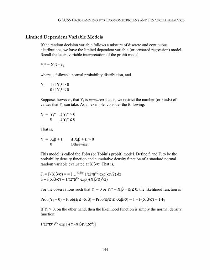
GAUSS PROGRAMMING FOR ECONOMETRICIANS AND FINANCIAL ANALYSTS
144
Limited Dependent Variable ModelsIf the random decision variable follows a mixture of discrete and continuousdistributions, we have the limited dependent variable (or censored regression) model.Recall the latent variable interpretation of the probit model,
Yi* = Xiβ + εi
where εi follows a normal probability distribution, and
Yi = 1 if Yi* > 00 if Yi* ≤ 0
Suppose, however, that Yi is censored-that is, we restrict the number (or kinds) ofvalues that Yi can take. As an example, consider the following:
Yi = Yi* if Yi* > 00 if Yi* ≤ 0
That is,
Yi = Xiβ + εi if Xiβ + εi > 00 Otherwise.
This model is called the Tobit (or Tobin’s probit) model. Define fi and Fi to be theprobability density function and cumulative density function of a standard normalrandom variable evaluated at Xiβ/σ. That is,
Fi = F(Xiβ/σ) = = ∫ - ∞ Xiβ/σ 1/(2π)1/2 exp(-z2/2) dz
fi = f(Xiβ/σ) = 1/(2π)1/2 exp(-(Xiβ/σ)2/2)
For the observations such that Yi = 0 or Yi* = Xiβ + εi ≤ 0, the likelihood function is
Prob(Yi = 0) = Prob(εi ≤ -Xiβ) = Prob(εi/σ ≤ -Xiβ/σ) = 1 – F(Xiβ/σ) = 1-Fi
If Yi > 0, on the other hand, then the likelihood function is simply the normal densityfunction:
1/(2πσ2)1/2 exp [-(Yi-Xiβ)2/(2σ2)]

DISCRETE AND LIMITED DEPENDENT VARIABLES
145
Therefore the likelihood function for the tobit model is a mixture of the above discreteand continuous distributions depending on the values taken by the dependent variable(i.e., zero or positive):
L = ∏i |Yi = 0(1-Fi) ∏i |Yi > 01/(2πσ2)1/2 exp [-(Yi-Xiβ)2/(2σ2)]
The corresponding log-likelihood function is
ll = ∑i |Yi = 0 ln(1-Fi) - ½ ∑i |Yi > 0 [ln(π)+ln(σ2)+(Yi-Xiβ)2/σ2]
Then, for the maximum likelihood estimation, we solve from the following first-orderconditions:
∂ll/∂β = - (1/σ) ∑i |Yi = 0 fiXi/(1-Fi) + (1/σ2) ∑i |Yi > 0(Yi-Xiβ)Xi = 0∂ll/∂σ2 = ½ (1/σ3) ∑i |Yi = 0 fiXiβ/(1-Fi) - ½ (1/σ2) ∑i |Yi > 0[1-(Yi-Xiβ)2/σ2] = 0
To interpret the estimated coefficients of the model, we may use three conditionalexpected values:
E(Yi*|Xi) = Xiβ
E(Yi |Xi,Yi>0) = Xiβ + E(εi |Yi > 0)= Xiβ + E(εi |εi > -Xiβ)= Xiβ + σ fi/Fi > E(Yi*|Xi)
E(Yi|Xi) = Fi E(Yi |Xi,Yi > 0)= Fi Xiβ + σ fi
The first expected value (corresponding to the “uncensored” case) is easy to obtain.The last expected value will be of particular interest if our sample contains many“censored” observations. Accordingly, for the j-th explanatory variable, thecorresponding marginal effects are:
∂E(Yi*|Xi)/∂Xij = βj
∂E(Yi|Xi,Yi>0)/∂Xij = βj [1- (Xiβ/σ)(fi/Fi) –(fi/Fi)2]
∂E(Yi|Xi)/∂Xij = Fi ∂E(Yi|Xi,Yi > 0)/∂Xij + E(Yi |Xi ,Yi > 0) ∂Fi/∂Xij
= Fi βj
We note that the last “censored” marginal effect differs from the first “uncensored”one by a scale factor equal to the probability of that observation not being censored.In other words, the scale factor is equal to Fi (recall that Fi is 1-Prob(Yi = 0)).

GAUSS PROGRAMMING FOR ECONOMETRICIANS AND FINANCIAL ANALYSTS
146
The tobit model is often estimated for comparison with the alternative probit or countmodel specifications. The model can be easily extended to consider more than onecensoring point. For instance, we could “censor” both tails of the distribution. This isan example of a doubly censored regression
Lesson 8.3: Tobit Analysis of Extramarital Affairs
This example is taken from Greene (1999, Example 20.12), which is based on Fair(1978). The study examines at the qualitative responses to a question aboutextramarital affairs from a sample of 601 men and women married for the first time.The dependent variable is:
Y Number of affairs in the past year: 0, 1, 2, 3, 4-10 (coded as 7), 11-365 (codedas 12).
The preponderance of zeros (no affairs) may not render the tobit model to be the bestfor the study. The complete data set used in the article is available from the text filefair.txt, but we present only the restricted model using a subset of five explanatoryvariables as follows:
Z2 Age.Z3 Number of years married.Z5 Degree of religiousness: 1 (anti-religious), …, 5 (very religious).Z7 Hollingshead scale of occupation: 1, …, 7.Z8 Self-rating of marriage satisfaction: 1 (very unhappy), …, 5 (very happy).
The regression equation is
Y = β0 + β2 Z2 + β3 Z3 + β5 Z5 + β7 Z7 + β8 Z8 + ε
The conclusion and interpretation of the estimated model are up to the interestedreaders. We emphasize here the implementation of tobit analysis using GPE andGAUSS. We need to briefly explain the maximum likelihood estimation procedure.Recall that the likelihood function of the tobit model is a mixture of discrete andcontinuous normal likelihoods, depending on the censored point (zero) of thedependent variable. Unlike in the probit model, the standard error is an explicitunknown parameter which must be estimated together with the regression parameters.In the following program, from line 22 to 28, the procedure tobitf defines the log-likelihood function for each sample observation. For maximum likelihood estimation,

DISCRETE AND LIMITED DEPENDENT VARIABLES
147
we need to set _nlopt=2 (line 10), which instructs GPE to maximize the sum of theindividual log-likelihood functions7.
123456
7
8
91011121314
151617181920
21
22232425262728
/*** Lesson 8.3: Tobit Analysis of Extramarital Affairs** Greene (1999), Example 20.12** See also R. Fair, JPE, 86, 1978, 45-61*/use gpe2;output file=gpe\output8.3 reset;n=602;load data[n,15]=gpe\fair.txt;y=data[2:n,13];z=data[2:n,5 6 8 11 12]; @ use z2, z3, z5, z7, z8 @
call reset;
@ Uncensored OLS estimation @call estimate(y,z);
@ Tobit model estimation @z=z~ones(rows(z),1); @ RHS variables inc. constant @_nlopt=2; @ using component likelihood function @_method=5;_iter=100;_b=__b|5.0;call estimate(&tobitf,y~z);
@ Tobit model interpretation based on E(y) @b=__b[1:6];s=__b[7];ey=cdfn(z*b/s).*(z*b)+s.*pdfn(z*b/s);em=cdfn(z*b/s).*b';print "Expected Value Marginal Effects";;print ey~em[.,1:5];
end;
/* Log-likelihood function: tobit model */proc tobitf(x,b);
local y,z,k;k=rows(b);y=x[.,1];z=(y-x[.,2:k]*b[1:k-1])/b[k];retp((y.==0).*ln(cdfn(z))+(y.>0).*ln(pdfn(z)/b[k]));
endp;
Remember that tobit is a nonlinear model. First, the uncensored model is estimated byordinary least squares (line 8). The estimated parameters are used as the initial valuesin the tobit model estimation (line 14). Here is the result of the estimated tobit model,which converges after 60 iterations.
7 Because the size of this nonlinear optimization is beyond the limit of GAUSS Light, theprofessional version of GAUSS should be used for Lesson 8.3.

GAUSS PROGRAMMING FOR ECONOMETRICIANS AND FINANCIAL ANALYSTS
148
Maximum Likelihood Estimation-----------------------------Number of Observations = 601Number of Parameters = 7
Maximum Number of Iterations = 100Step Size Search Method = 0Convergence Criterion = 0Tolerance = 0.001
Initial Result:Log Likelihood = -886.21Parameters = -0.050347 0.16185 -0.47632 0.10601 -0.712245.6082 5.0000
Using Quadratic Hill-Climbing Algorithm
Final Result:Iterations = 60 Evaluations = 1981497Log Likelihood = -705.58Parameters = -0.17933 0.55414 -1.6862 0.32605 -2.28508.1742 8.2471Gradient Vector = 3.0579e-005 3.0303e-006 2.2826e-006 1.4280e-006 2.3271e-006 4.5474e-007 -2.7294e-006
Asymptotic AsymptoticParameter Std. Error t-Ratio
X1 -0.17933 0.079136 -2.2661X2 0.55414 0.13459 4.1174X3 -1.6862 0.40378 -4.1761X4 0.32605 0.25443 1.2815X5 -2.2850 0.40787 -5.6022X6 8.1742 2.7419 2.9812X7 8.2471 0.55363 14.896
For interpretation of the estimated parameters, we compute the expected values ofcensored observations and the corresponding marginal effects of the explanatoryvariables (see lines 14-19). The computation is for each sample observation.
To save the space we do not list the 601 observations of expected values andmarginal effects. One alternative is to calculate the average of the estimated expectedvalues and marginal effects:
print meanc(ey~em[.,1:5])’;
A second alternative is to evaluate the expected values and marginal effects at themeans of the explanatory variables by inserting the following statement before line16:
z=meanc(z)’;

DISCRETE AND LIMITED DEPENDENT VARIABLES
149
We conclude with an important remark. In Lesson 8.3, the dependent variable isactually more like count data, rather than a continuous variable, recording the numbersof occurrences of extramarital affairs within a year. As a matter of fact, this model iswell-suited for probit analysis. If we define the dependent variable Y as a binaryvariable: 0 for no affairs, and 1 otherwise, then the same data set can be used foreither probit or logit analysis. However, the estimated parameters, expected values,and marginal effects of the probit (or logit) model are not directly comparable to thoseof the tobit model. The dependent variable being “explained” or “predicted” isdifferent under tobit estimation than under probit or logit estimation. With a tobitmodel, we are predicting the mean number of affairs. With a probit or logit model, weare predicting the probability of an affair occurring within a year. The probit analysisis not concerned with the actual number of affairs. We leave the model comparison tothe interested readers.


IX Heteroscedasticity
Heteroscedasticity is a common problem with cross-sectional data, in which unequalmodel variance is observed. Ordinary least squares estimation with a heterogeneouslydistributed error structure leads to inefficient estimates of the regression parameters.In order to correct for this inefficiency, the source of heteroscedasticity in relation toone or more variables must be identified.
To illustrate how to test and correct for the problem of heteroscedasticity, thefollowing relationship of public school spending (SPENDING) and income(INCOME) across 50 states in the U. S. is considered:
SPENDING = β0 + β1 INCOME + β2 INCOME2 + ε
To estimate this equation, which is used for all the lessons in this chapter, a cross-sectional data file greene.txt is used8. It gives per capita public school expenditureand per capita income by state in 1979. Let’s take a look at the data file greene.txt wewill be dealing with now. The data file contains three columns. The first column is thestate identifier (STATE), the second column is per capita expenditures on publicschools (SPENDING), and the third column is per capita income (INCOME).Viewing greene.txt in the Edit window reveals a problem with the data. Notice thatWI (Wisconsin) is missing a data observation. The row WI has “NA” for thecorresponding value in the SPENDING column. GAUSS sees “NA” as a characterstring, not suitable for numerical computation. GAUSS has commands that convertcharacter strings, such as “NA”, to a symbol that it can interpret as a missing value.The first part of each lesson in this chapter walks you through the process ofconverting greene.txt, with missing values, to useable data. Several new GAUSScommands are introduced for this purpose.
Heteroscedasticity-Consistent Covariance MatrixAssuming heteroscedasticity, the ordinary least squares estimator is unbiased butinefficient. We can keep the unbiased least squares estimator, but correct forinefficiency with an estimated heteroscedasticity-consistent covariance matrix. Lesson
8 This example was used in Greene (1997, Chapter 12), but it has been removed from theupdated fourth edition (Greene, 1999).

GAUSS PROGRAMMING FOR ECONOMETRICIANS AND FINANCIAL ANALYSTS
152
9.1 below demonstrates the use of the input control variable _hacv to correct thecovariance matrix.
Lesson 9.1: Heteroscedasticity-Consistent Covariance Matrix
In this lesson, we estimate the regression equation of public school spending(SPENDING) with regressors income (INCOME) and squared income (INCOME2)using the data file greene.txt.
For a heteroscedastic regression model, a consistent estimate of the variance-covariance matrix is obtained by approximating the original heteroscedastic varianceswith the squares of estimated residuals from ordinary least squares estimation. That is,
Var(β ^ ) = (X’X)-1(X’Σ ^ )X) (X’X)-1
where X is the data matrix of regressors, β ^ is the ordinary least squares estimator of
the parameters vector β, and Σ ^ is a diagonal variance-covariance matrix (i.e., theestimator of E(εε’)) with the elements being the squares of the estimated regressionresiduals.
From two least squares estimations, one with the ordinary variance-covariance matrixand the other with the heteroscedasticity-consistent covariance matrix, we can directlycompare the results of these regressions. In GPE, by setting the input variable_vcov=1 (see line 11 of Lesson 9.1), the details of the variance-covariance matrixare presented. The second regression estimation with newly introduced input variable_hacv=1 (see line 13 of Lesson 9.1) computes the heteroscedasticity consistentestimates of the variance-covariance matrix instead of the inefficient one from theordinary least squares.
123
45678
9
10
/*** Lesson 9.1: Heteroscedasticity-Consistent** Variance-Covariance Matrix*/use gpe2;output file = gpe\output9.1 reset;load greene[52,3]= gpe\greene.txt;
data = greene[2:52,.];data = miss(data,"NA"); @ NA to missing value @data = packr(data); @ deletes row w/miss value@spending = data[.,2];income = data[.,3]/10000;
call reset;
/* Ordinary Least Squares */_names = "spending","income","income^2";

HETEROSCEDASTICITY
153
1112
131415
_vcov = 1;call estimate(spending,income~income^2);
/* Ordinary Least Squares */_hacv = 1; @ with hetero. consistent var-cov @call estimate(spending,income~income^2);end;
Line 5 introduces the miss command of GAUSS. It modifies the matrix data bycomparing each element in the matrix data to the character string “NA”. If anelement in data equals “NA”, it is replaced with a dot “ . ”, GAUSS’s symbol for amissing value. In the next line, packr(data) deletes any rows that contain anymissing values in the matrix data. After data has been packed (line 6), the numberof rows in data is reduced to 50. Refer to GAUSS manual or on-line help to findmore information on the commands miss and packr used here.
Try combining lines 4, 5, and 6 for efficiency:
data=packr(miss(greene[2:52,.],"NA"));
The result of the first least squares estimation with the option to print out theestimated variance-covariance matrix (lines 10 to 12) is:
Least Squares Estimation------------------------Dependent Variable = SPENDINGEstimation Range = 1 50Number of Observations = 50Mean of Dependent Variable = 373.26Standard Error of Dependent Variable = 94.553
R-Square = 0.65534 R-Square Adjusted = 0.64068Standard Error of the Estimate = 56.679Log-Likelihood Function Value = -271.27Log Ammemiya Prediction Criterion (APC) = 8.1331Log Akaike Information Criterion (AIC) = 8.1329Log Schwarz Bayesian Information Criterion (BIC) = 8.2476
Sum of Squares SS DF MSS F Prob>FExplained 2.8709E+005 2 1.4355E+005 44.684 1.3445E-011Residual 1.5099E+005 47 3212.5Total 4.3808E+005 49 8940.3
Variable Estimated Standard t-Ratio Prob PartialName Coefficient Error 47 DF >|t| RegressionINCOME -1834.2 828.99 -2.2126 0.031820 0.094335INCOME^2 1587.0 519.08 3.0574 0.0036770 0.16590CONSTANT 832.91 327.29 2.5449 0.014275 0.12111
Variance-Covariance Matrix of CoefficientsINCOME 6.8722E+005INCOME^2 -4.2844E+005 2.6944E+005CONSTANT -2.7021E+005 1.6709E+005 1.0712E+005

GAUSS PROGRAMMING FOR ECONOMETRICIANS AND FINANCIAL ANALYSTS
154
INCOME INCOME^2 CONSTANT
Correlation Matrix of CoefficientsINCOME 1.0000INCOME^2 -0.99567 1.0000CONSTANT -0.99591 0.98352 1.0000
INCOME INCOME^2 CONSTANT
In order to compare the ordinary least squares estimates of standard errors and thevariance-covariance matrix with the heteroscedasticity-consistent variance-covariancematrix, we look at a portion of the output from the second regression estimation (lines13 and 14):
Variable Estimated Standard t-Ratio Prob PartialName Coefficient Error 47 DF >|t| RegressionINCOME -1834.2 1243.0 -1.4756 0.14673 0.044275INCOME^2 1587.0 829.99 1.9121 0.061968 0.072177CONSTANT 832.91 460.89 1.8072 0.077137 0.064972
Variance-Covariance Matrix of CoefficientsINCOME 1.5452E+006INCOME^2 -1.0296E+006 6.8889E+005CONSTANT -5.7170E+005 3.7941E+005 2.1242E+005
INCOME INCOME^2 CONSTANT
Correlation Matrix of CoefficientsINCOME 1.0000INCOME^2 -0.99796 1.0000CONSTANT -0.99789 0.99182 1.0000
INCOME INCOME^2 CONSTANT
In this example, the estimated heteroscedasticity-consistent standard errors and thevariance-covariance matrix of the regression parameters are both larger than theirordinary least squares counterparts. The results are more reliable but smaller t-ratios,leading to the conclusion of statistically insignificant parameter estimates. Suchcorrection to the model is useful when the problem of heteroscedasity is of unknownform.
Weighted Least SquaresAs mentioned earlier, if we can identify one or more of the regressors in the model asthe source of heterogeneity in the variances, then a variation of least squares calledWeighted Least Squares is recommended. This estimation method adjusts all dataseries across the regression equation in accordance with the origin of theheteroscedasticity. Lesson 9.2 details the Goldfeld-Quandt approach, while Lesson 9.3presents more general testing procedures devised by Breusch-Pagan and White.

HETEROSCEDASTICITY
155
Lesson 9.2: Goldfeld-Quandt Test and Correction for Heteroscedasticity
Continuing on with the spending-income regression equation of Lesson 9.1, thislesson introduces the Goldfeld-Quandt method to test for heteroscedasticity. It thencorrects for this condition by using the method of weighted least squares.
The Goldfeld-Quandt test requires data to be sorted according to the size of theindependent variable suspected to be the source of heteroscedasticity. The entire dataset is then divided into three parts, dropping the middle group, and running theregression using only the groups of smallest and largest values. Separate regressionsare estimated on each of the groups of smallest and largest values. Residual Sum ofSquares (RSS) from both groups are then compared in the Goldfeld-Quandt teststatistic.
As in the previous Lesson 9.1, the data is read from greene.txt and is corrected formissing values. The Goldfeld-Quandt test requires a sorted data series in accordancewith the suspected source of heteroscedasticity. Sorting the rows in the matrix, data,by the information in the third column (that is, the variable INCOME) is done in line7. INCOME is sorted from its smallest value to its largest. The GAUSS Help menugives greater details about the data sorting commands such as sortc used here.
123
456789
10
1112131415
16171819
20
/*** Lesson 9.2: Goldfeld-Quandt Test and** Correction for Heteroscedasticity*/use gpe2;output file = gpe\output9.2 reset;load greene[52,3]= gpe\greene.txt;
data = greene[2:52,.];data = miss(data,"NA"); @ NA to missing value @data = packr(data); @ deletes row w/miss value @data = sortc(data,3); @ sort data (income), in ascending order @spending = data[.,2];income = data[.,3]/10000;
call reset;
/* Goldfeld-Quandt Test */_names = "spending","income","income^2";_begin = 1;_end = 17;call estimate(spending,income~income^2);mss1 =__rss/14; @ N-K = 17-3 = 14 @
_begin = 34;_end = 50;call estimate(spending,income~income^2);mss2 =__rss/14; @ N-K = 17-3 = 14 @
print "Goldfeld-Quandt Test Statistic = " mss2/mss1;
/* Weighted Least Squares */

GAUSS PROGRAMMING FOR ECONOMETRICIANS AND FINANCIAL ANALYSTS
156
21222324
call reset;_weight = 1/income;call estimate(spending,income~income^2);end;
Selecting the first group of the17 smallest observations to regress for the Goldfeld-Quandt test is done by restricting the data matrix to only include observations from 1to 17 (lines 12 and 13). The use of the output control variable, __rss, is introducedin line 15. __rss stores the sum of squared residuals from the latest regressionestimation. Each time when the procedure estimate is called, output controlvariables are assigned new values. To save the value of __rss/14, mean sumsquares of residuals, for later use in the Goldfeld-Quandt test statistic, it is assigned tovariable mss1. Similarly, lines 16, 17, and 18, select the 17 largest observations andrun the regression, assigning the resulting __rss/14 to the variable mss2.
Since we are only interested in the RSS from the regressions, the outputs from the firsttwo estimations are not printed here. Instead, the result of Goldfeld-Quandt teststatistic from line 20 is given as follows:
Goldfeld-Quandt Test Statistic = 1.9444
This statistic is computed according to the formula:
RSS2N2-KRSS1N1-K
which follows the F-distribution with N2-K and N1-K degrees of freedom, where N1and N2 are the number of observations corresponding to the two separate samples,and K is the number of regressor parameters, including constant. Since the Goldfeld-Quandt method requires that the test statistic be greater than 1, the largest RSS (RSS2)must be in the numerator. The computed value of 1.94 is smaller than the criticalvalue of F(14,14) at a 5 % level of significance (that is, 2.40), so we could not rejectthe hypothesis of homoscedasticity.
Although there seems to be no problem of heteroscedasticity in the spending-incomeequation based on the Goldfeld-Quandt test, we warn the reader to never totally relyon statistical results from just one single test. We continue on to show you theweighted least squares method for correcting heteroscedasticity.
The problem of heteroscedasticity is corrected using weighted least squares. In line22, the statement:

HETEROSCEDASTICITY
157
_weight = 1/income;
tells GPE to estimate the model using 1/INCOME as the weight incorporated in theregression estimation called on line 23. All the variables, both dependent andindependent, including constant term, are weighted (or divided by income). Therationale is that the variable INCOME2 may be used to approximate the heterogeneousvariances of the model.
Because input variables _begin and _end had been set to non-default values earlierin the program, calling reset again (line 21) is the simplest way to insure that allcontrol variables are reset to their default values for the new estimation to come.
Delete line 21 or change it to
@ call reset; @
See what happens. Why?
The regression output corrected for heteroscedasticity is available in the output fileoutput9.2. Compare the earlier ordinary least squares estimation with theheteroscedasticity consistent covariance matrix from Lesson 9.1,
SPENDING = 832.91 - 1834.2 INCOME + 1587.0 INCOME2
s.e. (460.89) (1243.0) (829.99)
with the weighted least squares estimation using 1/INCOME as the weightingvariable,
SPENDING = 664.58 - 1399.3 INCOME + 1311.3 INCOME2
s.e. (333.61) (872.07) (563.71)
Notice that numbers in parentheses are the estimated standard errors of thecoefficients. The results of the two regressions are similar, but in theory, weightedleast squares estimation is more efficient.
Lesson 9.3: Breusch-Pagan and White Tests for Heteroscedasticity
In this lesson, we will explain briefly other methods to test for heteroscedasticity, theBreusch-Pagan and White tests for general heteroscedasticity. Many econometricsreferences cover the operation of this test in more detail.
In an auxiliary regression, Breusch-Pagan test for general heteroscedasticity using allexplanatory variables including constant term as the regressors to compute the teststatistic. The test procedure does not rely on any particular variable or functional form

GAUSS PROGRAMMING FOR ECONOMETRICIANS AND FINANCIAL ANALYSTS
158
to specify heteroscedasticity. In addition, it does not require the data to be sorted.However, the Breusch-Pagan test does assume residual normality for accurate results.The alternative Koenker-Basset test is more forgiving in regards to the assumption ofnormality.
The White test is based on the computation of heteroscedasiticity consistentcovariance matrix as described in Lesson 9.1, in which the explanatory variables andtheir squares and cross products are used to fit the squared residuals in a regrssionsetting. The resulting goodness of fit is the test statistic.
We note that both the Breusch-Pagan and White tests for general heteroscedasticity donot offer the information of the source and the form of heteroscedasticity. To correctfor the problem, more specific heteroscedastic strucutre of the model may be required.It is quite easy to implement the Breusch-Pagan and White tests for heteroscedasticityin GPE. What you need is to set a posstive value to the input control variable_bptest.
123
45678
9
10111213
14
/*** Lesson 9.3: Breusch-Pagan and White Tests** for Heteroscedasticity*/use gpe2;output file = gpe\output9.3 reset;load greene[52,3]= gpe\greene.txt;
data = greene[2:52,.];data = miss(data,"NA"); @ NA to missing value @data = packr(data); @ deletes row w/mis value @spending = data[.,2];income = data[.,3]/10000;
call reset;
/* Breusch-Pagan and White Tests */_names = "spending","income","income^2";_bjtest = 1;_bptest = 1;call estimate(spending,income~income^2);
end;
Lines 1 through 10 are similar to Lesson 9.1. Keeping in mind that the working of theBreusch-Pagan test assumes that residuals are normally distributed, we have includedthe Bera-Jarque test for residual normality on line 11 (_bjtest=1). Line 12(_bptest=1) performs the Breusch-Pagan and White tests for generalheteroscedasticity.
Let’s examine the output now. The regression result from the first estimation (line 13)is the same as the result discussed in the previous Lesson 9.2, with additional pieces of

HETEROSCEDASTICITY
159
information: Bera-Jarque test for normality, Breusch-Pagan and White tests forheteroscedasticity:
Bera-Jarque Wald Test for NormalityAsymptotic Standard Error of Residuals = 54.952Skewness of Residuals = -0.083322Kurtosis of Residuals = 3.3877Chi-Sq( 2) Prob>Chi-Sq
0.37107 0.83066
Breusch-Pagan and White LM Tests for HeteroscedasticityChi-Sq DF Prob>Chi-Sq
Breusch-Pagan Test 18.903 2 7.8553e-005Koenkar-Basset Test 15.834 2 0.00036454White Test 21.159 4 0.00029443
Result of the Bera-Jarque test reveals normality in the residuals (refer to Lesson 3.6for details on the Bera-Jarque test for residual normality). The last section of theregression output is what we are interested in, the Breusch-Pagan and White tests forheteroscedasticity. It is set up to test the null hypothesis of homoscedasticity. That is,for the Breusch-Pagan test, if the computed test value is less than the critical value ofthe Chi-square distribution with two degrees of freedom, we fail to reject thehypothesis that the model error is homogeneously distributed. Similar conclusion isobtained from the White test, which is based on the R2 statistic of the auxilaryregression with 4 degrees of freedom. Note the low P-values for both Breusch-Paganand White test statistics leading us to reject the hypothesis of homoscedasticity andconclude that heteroscedasticity exits in the model.
Remember the requirement of residual normality for the Breusch-Pagan test? If theresiduals are not normally distributed, we need to use a more general version of theBreusch-Pagan test, called the Koenkar-Basset test. The closer to normal theresiduals are, the more similar are these two test statistics. If absolute normalityexists, the computed values of the two tests will be identical. Since the estimatedresiduals are indeed normally distributed for this example as shown earlier, both testsreturn rather close values, 18.9 and 15.8, respectively. Our conclusion ofheteroscedasticity is the same from both Breusch-Pagan and Koenkar-Basset teststatistics.
Nonlinear Maximum Likelihood EstimationA more general approach is to consider the regression model, linear or nonlinear, withthe heteroscedastic variance-covariance matrix
∑ = σ2Ω

GAUSS PROGRAMMING FOR ECONOMETRICIANS AND FINANCIAL ANALYSTS
160
where Ω is a positive diagonal matrix representing the proportional variance weight ofeach data observation. It is impossible to estimate the general matrix Ω. Usually Ω isre-parameterized with a vector α of only a few parameters. By assuming normalprobability distribution for the model’s error term, maximum likelihood estimation isimplemented to estimate the regression parameters and heteroscedastic variances.
Consider a sample of N data observations Z = [Y,X] in fitting the regression modelF(Z,β) = ε, where Y is the left-hand-side dependent variable, X is the right-hand-sideindependent variables, and β is the unknown parameters. For each data observation i,let εi(β) = F(Zi,β) and assume εi(β) is normally independently distributed with zeromean and positive variance σi
2. The log-likelihood function, ll(β,σσσσ2) =ll(β,σ1
2,σ22,…,σN
2) for brevity, is
ll(β,σσσσ2) = -N/2 ln(2π) - ½ ∑i=1,2,…,N ln(σi2) - ½ ∑i=1,2,…,N (εi(β)2 / σi
2)
Given the general form of heteroscedasticity, there are too many unknown parameters.For practical purpose, some hypothesis of heteroscedasticity must be assumed:
σi2 = σ2 h(Xi,α)
where σ2 > 0 and the heteroscedastic function h depends on part or all of theregressors and a vector of parameters α. Given a specific formulation ofheteroscedasticity, hi(α) = h(Xi,α) for brevity, the log-likelihood function is written as:
ll(β,α,σ2) = -N/2 (ln(2π) + ln(σ2))
- ½ ∑i=1,2,…,N ln(hi(α)) - 1
2σ2 ∑i=1,2,…,N (εi(β)2 / hi(α))
Let εi*(β,α) = εi(β) / hi(α) and substitute out σ2 with ε*(β,α)’ε*(β,α)/N, then theconcentrated log-likelihood function is
ll*(β,α) = -N/2 (1 + ln(2π) + ln(ε*(β,α)’ε*(β,α)/N)) - ½ ∑i=1,2,…,N ln(hi(α))
As the variances must be explicitly estimated, σi2 = σ2 hi(α), the objective log-
likelihood function is inevitably complicated. To maximize the log-likelihoodfunction, techniques of nonlinear optimization of Chapter VI are applicable.
Consider the following examples of heteroscedasticity specifications, in which X isassumed to be a single variable for simplicity. The corresponding functional forms ofh(α) and ε* are defined for the concentrated log-likelihood function:
ll*(β,α) = -N/2 (1 + ln(2π) + ln(ε*’ε*/N)) - ½ ∑i=1,2,…,N ln(hi(α))

HETEROSCEDASTICITY
161
σi2 hi(α) εi*
1. σ2(Xiα) Xiα εi / (Xiα)½ (Note: Xiα > 0)2. σ2(Xiα)2 (Xiα)2 εi / Xiα3. σ2exp(Xiα) exp(Xiα) εi / exp(Xiα)½
4. σ2(Xiα) Xi
α εi / Xiα/2
The last two cases may be expressed in log form:
3. ln(σi2)= ln(σ2) + α Xi
4. ln(σi2)= ln(σ2) + α ln(Xi)
Depending on whether the variable X is log-transformed or not, both cases ofmultiplicative heteroscedasticity are essentially the same. For (3) and (4), if α = 0 themodel is homoscedastic. If α = 2, we have case (2).
Lesson 9.4: Multiplicative Heterscedasticity
Let’s re-examine the heteroscedastic relationship of public school spending(SPENDING) and income (INCOME) of the previous three lessons:
SPENDING = β0 + β1 INCOME + β2 INCOME2 + ε
The data set is given in greene.txt. This time we will find and compare the maximumlikelihood estimates based on the following hypothesis of multiplicativeheterscedasticity:
σi2 = σ2 INCOMEi
α
Lesson 9.2 has demonstrated the weighted least squares estimation for the case of α =2. The alternative expression of multiplicative heteroscedasticity is
σi2 = σ2 exp(α INCOMEi)
If the variable INCOME is in log form for the alternative expression ofheteroscadasticity, the two forms of multiplicative heteroscedasticity are the same.
1234
/*** Lesson 9.4: Multiplicative Heteroscedasticity** Greene (1997), Chap. 12.5*/use gpe2;output file=gpe\output9.4 reset;load data[52,3]=gpe\greene.txt;data=data[2:52,2]~(data[2:52,3]/10000); @ scale data @

GAUSS PROGRAMMING FOR ECONOMETRICIANS AND FINANCIAL ANALYSTS
162
56
789101112
13
14
151617181920
21222324
data=packr(miss(data,"NA")); @ take care of missing obs @b=data[.,1]/(ones(rows(data),1)~data[.,2]~(data[.,2]^2));
call reset;_method=4;_iter=100;_restart=10;_b=b|2.0;_nlopt=1;
call estimate(&llf,data);
end;
proc llf(data,b);local n,y,x,e,h,ll;y=data[.,1]; @ public school spending @x=data[.,2]; @ income @n=rows(y);h=x^b[4]; @ multiplicative hetero @
/*h=exp(b[4]*x);
*/e=(y-b[1]-b[2]*x-b[3]*(x^2))./sqrt(h);ll=-0.5*n*(1+ln(2*pi)+ln(e'e/n))-0.5*sumc(ln(h));retp(ll);
endp;
The first part of the program loads and scales the data, which is the same as inprevious lessons. Line 6 computes the linear model estimates as the starting values ofparameters for nonlinear maximum likelihood estimation (see line 11). The objectivelog-likelihood function llf is defined in lines 15 through 23. The specific form ofmultiplicative heteroscedasticity is given in line 20. Since the estimation hasexperienced some difficulty to improve the function value in its final iterations, we set_restart=10 in line 10 to restart the iteration in case of failure. If you have troubleunderstanding what this program is doing, a review of Chapter VI and the programlessons on nonlinear models there is recommended.
The result of maximum likelihood estimation is given in the following:
Non-Linear Optimization: Maximization Problem---------------------------------------------Assuming Maximum Likelihood FunctionNumber of Observations = 50Number of Parameters = 4
Maximum Number of Iterations = 100Step Size Search Method = 0Convergence Criterion = 0Tolerance = 0.001
Initial Result:Function Value = -268.70Parameters = 832.91 -1834.2 1587.0 2.0000

HETEROSCEDASTICITY
163
Using Newton-Raphson AlgorithmIteration = 1 Step Size = 1.0000 Value = -268.11Parameters = 563.08 -1141.3 1150.6 3.2550Iteration = 2 Step Size = 1.0000 Value = -268.09Parameters = 560.95 -1124.8 1132.8 3.2986Iteration = 3 Step Size = 1.0000 Value = -268.09Parameters = 560.69 -1124.1 1132.4 3.2985Iteration = 4 Step Size = 1.0000 Value = -268.09Parameters = 560.69 -1124.1 1132.4 3.2984Iteration = 5 Step Size = 1.0000 Value = -268.09Parameters = 560.69 -1124.1 1132.4 3.2985
Final Result:Iterations = 5 Evaluations = 126Function Value = -268.09Parameters = 560.69 -1124.1 1132.4 3.2985Gradient Vector = 2.0276e-008 0.00000 0.00000 1.7233e-006Hessian Matrix =
-0.020623 -0.014837 -0.010848 -0.00024046-0.014837 -0.010848 -0.0080655 9.0987e-005-0.010848 -0.0080655 -0.0061037 -0.00013901
-0.00024046 9.0987e-005 -0.00013901 -0.58515
AsymptoticParameter Std. Error t-Ratio
X1 560.69 354.11 1.5834X2 -1124.1 943.28 -1.1917X3 1132.4 621.04 1.8233X4 3.2985 1.3790 2.3920
The estimated public school spending-income relationship is summarized as:
SPENDING = 560.69 - 1124.1 INCOME + 1132.4 INCOME2
s.e. (354.11) (943.28) (621.04)
In addition, the heteroscedastic variance is related to the variable INCOME asfollows:
σi2 = σ2 INCOMEi
3.3
It is easy to modify Lesson 9.4 for the alternative (exponential) form of multiplicativeheteroscedasticity. Line 20 in the definition of log-likelihood function would bereplaced by:
h=exp(b[4]*x);
which is currently ignored by GAUSS within the comment notations (/* */). Make thechange and run the modified program. The resulting regression equation looks likethis:
SPENDING = 544.53 - 1076.2 INCOME + 1097.7 INCOME2

GAUSS PROGRAMMING FOR ECONOMETRICIANS AND FINANCIAL ANALYSTS
164
s.e. (364.97) (974.17) (643.10)
and the variance equation is:
σi2 = σ2 exp(4.23 INCOMEi)
Refer to the output file generated from the program and verify the above regressionresults. To summarize the discussion of heteroscedastic regression models, we puttogether and compare the estimation results of the public school spending-incomerelationship:
SPENDING = β0 + β1 INCOME + β2 INCOME2 + ε
(1)Lesson 9.1
(2)Lesson 9.2
(3)Lesson 9.4
(4)Lesson 9.4
β1 -1834.2(1243.0)
-1399.3(872.07)
-1124.1(943.28)
-1076.2(974.17)
β2 1587.0(829.99)
1311.3(563.71)
1132.4(621.04)
1097.7(643.10)
β0 832.91(460.89)
664.58(333.61)
560.69(354.11)
544.53(364.97)
α 0 2 3.2985(1.3790)
4.2344(1.7364)
The numbers in parentheses are the estimated standard errors of the parameters. Torecap the essence of each model, (1) Lesson 9.1 is an ordinary least squares withheteroscedasticity-consistent variance-covariance matrix; (2) Lesson 9.2 is a weightedleast squares using 1/INCOME as the weight (i.e., σi
2 = σ2 INCOMEi2); (3) and (4)
are the maximum likelihood estimators with multiplicative heteroscedasticity (i.e., σi2
= σ2 INCOMEiα and σi
2 = σ2 exp(α INCOMEi), respectively) as presented in Lesson9.4.
Which one is more accurate? We leave that decision to you.

XAutocorrelation
Autocorrelation is a problem most likely associated with time series data. It concernsthe relationship between previous and current error terms in a regression model. In thesimplest case, the serial correlation is of first order where the correlation betweencurrent and immediate previous errors is nonzero. The more complicated errorstructure can include autoregressive and moving average terms.
Ordinary least squares estimation with autocorrelated error structure results in a lossof efficiency. Therefore, statistical inference using t and F test statistics cannot betrusted.
In this chapter, we revisit the multiple regression model of U. S. production function,using labor (L), capital (K), and output (X) data series of cjx.txt:
ln(X) = β0 + β1 ln(L) + β2 ln(K) + ε
Lesson 10.1 below demonstrates the use of the input control variable _hacv to obtaina consistent estimator of the variance-covariance matrix, when ordinary least squaresis used. Several tests for the existence of autocorrelation are given in Lesson 10.2.Correction methods for first order autocorrelation to improve the efficiency ofparameter estimates are presented in Lessons 10.3 and 10.4. Since a more complicatedstructure of autocorrelation may be identified, the estimation of autoregressive andmoving average error structures is considered in the last three lessons. Lesson 10.5 isa model with higher order autocorrelation. The techniques of maximum likelihood isintroduced in Lesson 10.6, while Lesson 10.7 covers the nonlinear method.
Autocorrelation-Consistent Covariance MatrixGiven the existence of autocorrelation in a regression equation, the ordinary leastsquares estimator is unbiased but inefficient. Following from the treatment of theheteroscedasticity-consistent covariance matrix introduced in the previous chapter, wecan keep the unbiased parameter estimators but correct for the variance-covarianceestimator with an autocorrelation-consistent covariance matrix. Combining bothproblems of heteroscedasticity and autocorrelation, the Newey-West estimator ofheteroscedasticity autocorrelation consistent covariance matrix is a simple approach todeal with an unspecified structure of heteroscedasticity and autocorrelation. The

GAUSS PROGRAMMING FOR ECONOMETRICIANS AND FINANCIAL ANALYSTS
166
drawback is that the order of autocorrelation must be predetermined for thecomputation of Newey-West estimators.
For a regression model with an unspecified structure of heteroscedasticity andautocorrelation, the consistent estimator of the variance-covariance matrix is
Var(β ^) = (X’X)-1 (X’Σ ^ X)(X’X)-1
where X is the data matrix of regressors, β ^ is the ordinary least squares estimator of the
parameter vector β, and Σ ^ is the Newey-West covariance estimator for autocorrelatedand possibly heterogeneous disturbances. Refer back to Lesson 9.1 for more details onthe consistent covariance matrix in the context of heteroscedasticity.
Lesson 10.1: Heteroscedasticity-Autocorrelation-Consistent Covariance Matrix
Based on the Cobb-Douglas production model for U. S. manufacturing introduced inLesson 3.4, we first repeat the ordinary least squares estimation, printing out the OLSvariance-covariance matrix. Then two more least squares estimations are performed,one with an estimated autocorrelation-consistent covariance matrix and the other witha heteroscedasticity-autocorrelation-consistent covariance matrix. Thus, we candirectly compare the results of these regression estimations.
Here is the program:
123
4567
8
91011
1213
/*** Lesson 10.1: Heteroscedasticity Autocorrelation** Consistent Variance-Covariance Matrix*/use gpe2;output file = gpe\output10.1 reset;load data[40,6]= gpe\cjx.txt;
year = data[2:40,1];X = ln(data[2:40,2]);L = ln(data[2:40,3]);K = ln(data[2:40,5]);
call reset;
/* Ordinary Least Squares */_names = "X","L","K";_vcov = 1;call estimate(X,L~K);
/* Ordinary Least Squares */_hacv = 0,4;@ with auto consistent var-cov @call estimate(X,L~K);
/* Ordinary Least Squares */

AUTOCORRELATION
167
141516
_hacv = 1,4;@ w/hetero auto consist var-cov @call estimate(X,L~K);end;
Recall that by setting the GPE input variable _vcov = 1 (see line 10), the estimatedvariance-covariance matrix is presented. Instead of using the inefficient variance-covariance matrix from ordinary least squares, computation of the consistentcovariance matrix is controlled by the input variable _hacv. _hacv is either a scalaror a two-element vector. The first element of _hacv is reserved for heteroscedasicitycorrection as shown in Lesson 9.1 earlier, while the second element is the order ofautocorrelation to be considered for the estimator of an autocorrelation-consistentvariance-covariance matrix. Therefore, line 12 of the program:
_hacv = 0,4;
will compute the 4th-order autocorrelation-consistent variance-covariance matrix. Themixture of heteroscedasticity and a 4th-order autocorrelation consistent covariancematrix is obtained by setting line 14 to:
_hacv = 1,4;
Why the 4th-order autocorrelation correction? There is no particular reason for thischoice. As a matter of fact, we should try different numbers of orders to compute allthe consistent covariance matrices, to find the proper order that stabilizes theresulting covariance matrix.
We now analyze the output of three regression estimations. The first least squaresestimation with the option to print out the estimated variance-covariance matrix (lines10 to 11) is as follows:
Least Squares Estimation------------------------Dependent Variable = XEstimation Range = 1 39Number of Observations = 39Mean of Dependent Variable = 5.6874Standard Error of Dependent Variable = 0.46096
R-Square = 0.99463 R-Square Adjusted = 0.99433Standard Error of the Estimate = 0.034714Log-Likelihood Function Value = 77.286Log Ammemiya Prediction Criterion (APC) = -6.6471Log Akaike Information Criterion (AIC) = -6.6474Log Schwarz Bayesian Information Criterion (BIC) = -6.5195
Sum of Squares SS DF MSS F Prob>FExplained 8.0310 2 4.0155 3332.2 1.3921E-041Residual 0.043382 36 0.0012051Total 8.0744 38 0.21248
Variable Estimated Standard t-Ratio Prob Partial

GAUSS PROGRAMMING FOR ECONOMETRICIANS AND FINANCIAL ANALYSTS
168
Name Coefficient Error 36 DF >|t| RegressionL 1.4508 0.083228 17.431 3.9260E-019 0.89407K 0.38381 0.048018 7.9930 1.7130E-009 0.63960CONSTANT -3.9377 0.23700 -16.615 1.8332E-018 0.88464
Variance-Covariance Matrix of CoefficientsL 0.0069270K -0.0038020 0.0023057CONSTANT -0.018806 0.0092666 0.056169
L K CONSTANT
Correlation Matrix of CoefficientsL 1.0000K -0.95134 1.0000CONSTANT -0.95338 0.81428 1.0000
L K CONSTANT
Since autocorrelation is suspected for most time series data, the second regressionestimation (lines 12 and 13) is carried out with the 4th-order autocorrelation-consistentstandard errors and variance-covariance matrix:
Variable Estimated Standard t-Ratio Prob PartialName Coefficient Error 36 DF >|t| RegressionL 1.4508 0.10980 13.213 2.2423E-015 0.82905K 0.38381 0.058368 6.5756 1.1907E-007 0.54568CONSTANT -3.9377 0.33421 -11.782 6.5278E-014 0.79407
Variance-Covariance Matrix of CoefficientsL 0.012055K -0.0060940 0.0034069CONSTANT -0.035362 0.016267 0.11170
L K CONSTANT
Correlation Matrix of CoefficientsL 1.0000K -0.95089 1.0000CONSTANT -0.96366 0.83388 1.0000
L K CONSTANT
Finally, heteroscedasticity and the 4th-order autocorrelation-consistent covariancematrix is the outcome of the last regression estimation (lines 13 and 14):
Variable Estimated Standard t-Ratio Prob PartialName Coefficient Error 36 DF >|t| RegressionL 1.4508 0.11561 12.549 1.0409E-014 0.81392K 0.38381 0.062253 6.1653 4.1818E-007 0.51358CONSTANT -3.9377 0.33788 -11.654 8.9304E-014 0.79048
Variance-Covariance Matrix of CoefficientsL 0.013366K -0.0069673 0.0038755CONSTANT -0.037946 0.018529 0.11416

AUTOCORRELATION
169
L K CONSTANT
Correlation Matrix of CoefficientsL 1.0000K -0.96804 1.0000CONSTANT -0.97140 0.88092 1.0000
L K CONSTANT
Putting together the estimated regression equations with the three sets of estimatedstandard errors, we have
ln(X) = -3.94 + 1.45 ln(L) + 0.38 ln(K)s.e. (ols) (0.24) (0.08) (0.05)s.e. (ac) (0.33) (0.11) (0.06)s.e. (hac) (0.34) (0.12) (0.06)
In general, the consistent estimators of the covariance matrix are larger than theirordinary least squares counterparts. The consequence is a higher probability of type IIerror, or accepting the null hypothesis for the estimators. In this example, all threeestimated variance-covariance matrices of the coefficients are quite similar in spite ofthe consistency correction for autocorrelation and heteroscedasticity.
Detection of AutocorrelationGiven each observation of a linear regression model
Yi = Xi β + εi
the linear form of autocorrelated errors is written as:
ε i = ρ1ε i-1 + ρ2ε i-2 +…+ ρpεi-p + υi
where Y is the dependent variable, X is a vector of explanatory independent variablesand β is the associated parameter vector. The simplest case of autocorrelated errorstructure is autocorrelation of order 1, where p = 1, or AR(1). It is always worthwhileto check for the existence of autocorrelation before considering correcting theproblem.
Lesson 10.2: Tests for Autocorrelation
This lesson explores several methods to test for autocorrelation. The most popular testis the Durbin-Watson Bounds test, which is designed to check for first order serialcorrelation. The convenience of the Durbin-Watson Bounds test has its limits: it testsonly for first order autocorrelation and the regression must include a constant term.

GAUSS PROGRAMMING FOR ECONOMETRICIANS AND FINANCIAL ANALYSTS
170
Additionally, there cannot be lagged dependent variables in the regression equation.The Breusch-Godfrey LM test is more forgiving: lagged dependent variables may beincluded and it can be used to test for higher orders of autocorrelation. Checking theautocorrelation and partial autocorrelation coefficients can reveal a more complicatedautoregressive and moving average structure, of autocorrelated errors. This isaccomplished with the Box-Pierce and Ljung-Box Q test statistics. However, exceptfor the Durbin-Watson Bounds test, all tests for autocorrelation need a large samplesize to be useful.
The popular Durbin-Watson test statistic is a part of the residual statistics outputreported with the regression estimation. That is, it is available with the statement:
_rstat = 1;
To call the Breusch-Godfrey LM test statistic, we need to specify the order ofautocorrelation to be tested. Indeed, this is a cumulative test for no serial correlationup to the order specified. Therefore, we need only to find the autocorrelation at arather low order to confirm the problem. For example, to test for autocorrelation up tothe 4th order, use the statement:
_bgtest = 4;
Autocorrelation and partial autocorrelation coefficients are typically computed andplotted for a long period of lags. By examining these coefficients and theirdistribution, a pattern of autoregressive and moving average structures ofautocorrelated residuals may be identified. The Chi-square based Box-Pierce andLjung-Box Q test statistics work the same way as the Breusch-Godfrey LM test. Forexample, 12-lag autocorrelation and partial autocorrelation functions are called withthe statement:
_acf = 12;
The selection of the 4th-order autocorrelation for the Breusch-Godfrey LM test isonly a suggestion. What we need is the lowest number of orders to test forautocorrelation. Again, the use of 12 lags for calculating and plotting autocorrelationand partial autocorrelation coefficients is arbitrary. As a rule of thumb, about onequarter of the sample size should offer sufficient information concerning the sampleautocorrelation.
Here is the program:
123
/*** Lesson 10.2: Tests for Autocorrelation*/use gpe2;output file = gpe\output10.2 reset;load data[40,6]= gpe\cjx.txt;

AUTOCORRELATION
171
45678
9101112131415
year = data[2:40,1];X = ln(data[2:40,2]);L = ln(data[2:40,3]);K = ln(data[2:40,5]);call reset;
_names = "X","L","K";_rstat = 1;_rplot = 2;_bgtest = 4; @ Breusch-Godfrey, 4th order @_acf = 12; @ auto & partial auto,12 lags @call estimate(X,L~K);end;
Looking at the program, the use of input control variables _bgtest (line 12) and_acf (line 13) are new. You may set the value of _bgtest to any order ofautocorrelation for the Breusch-Godfrey LM test, in this case up to 4 orders are tested.Similarly, for calculating and plotting autocorrelation and partial autocorrelationfunctions, the number of lags must be given to the variable _acf. In this example, 12lags seem sufficient for a data size of about 40 observations.
Let’s analyze the first part of the estimation result (which is the same as that of Lesson10.1), paying attention to the Durbin-Watson test statistic:
Squared Correlation of Observed and Predicted = 0.99463Sum of Squared Residuals = 0.043382Sum of Absolute Residuals = 0.96779Sum of Residuals = -9.88614E-011First-Order Rho = 0.57053Durbin-Watson Test Statistic = 0.85808
The First-Order Rho is the estimated first-order serial correlation coefficient (ρ) whichranges from –1 to 1. At a value of 0.57 we can see that autocorrelation is a problem.To test the statistical significance of ρ = 0, the Durbin-Watson Bounds test is usedhere. The computed Durbin-Watson statistic of 0.858 lies below the lower boundcritical value of 1.382 for a regression using 39 observations and 2 explanatoryvariables (not including constant term) at a 5% level of significance.
The second part of the result concern the Breusch-Godfrey LM test of autocorrelation,up to the 4th-order:
Breusch-Godfrey LM Test for AutocorrelationChi-Sq DF Prob>Chi-Sq
AR( 1) 13.205 1 0.00027923AR( 2) 20.331 2 3.8471e-005AR( 3) 22.221 3 5.8666e-005AR( 4) 22.445 4 0.00016339

GAUSS PROGRAMMING FOR ECONOMETRICIANS AND FINANCIAL ANALYSTS
172
The Breusch-Godfrey LM test is compared with the critical value of the Chi-squaredistribution with degrees of freedom equal to the number of orders of autocorrelation.P-values of each order tested are given to simplify the analysis. It becomes clear thatautocorrelation exists from the very first order upward. Since the first order exhibitsthe problem of serial correlation as the Durbin-Watson Bounds test suggests, all LMtests for cumulative higher orders will certainly also identify autocorrelation.
The last part of the output lists and displays autocorrelation and partial autocorrelationcoefficients for regression residuals up to 12 lags. Standard errors of these coefficientsare useful to spot the significance of lags for autoregressive and moving averagestructures of autocorrelated residuals. In addition, both Box-Pierce and Ljung-Box Qtest statistics are computed for each lag. Similar to the Breusch-Godfrey LM test,these accumulative tests follow a Chi-square distribution with degrees of freedomcorresponding to each individual number of lags, adjusted for the number ofregression coefficients whenever necessary.
Autocorrelation and Partial Autocorrelation FunctionsARMA Model SpecificationMean = -2.8701e-012 Standard Error = 0.033788
Lag AR S.E.(AR) PAR S.E.(PAR) Box-Pierce Ljung-Box1 0.55892 0.20411 0.55892 0.16013 12.183 13.1452 -0.046422 0.20438 -0.52183 0.16013 12.267 13.2383 -0.19341 0.20902 0.27527 0.16013 13.726 14.9004 0.054712 0.20939 0.12555 0.16013 13.843 15.0375 0.20105 0.21428 -0.093386 0.16013 15.419 16.9376 0.047409 0.21455 -0.073459 0.16013 15.507 17.0467 -0.20382 0.21946 -0.12344 0.16013 17.127 19.1228 -0.32496 0.23147 -0.18444 0.16013 21.246 24.5699 -0.20559 0.23610 0.043822 0.16013 22.894 26.82210 -0.15817 0.23881 -0.36648 0.16013 23.870 28.20211 -0.23694 0.24476 -0.047891 0.16013 26.059 31.40712 -0.24987 0.25121 0.010437 0.16013 28.494 35.105
Both moving average and autoregressive processes of lower orders are visiblyidentifiable from the significant values of autocorrelation and partial autocorrelationcoefficients, respectively. These include the first lag of autocorrelation as well as thefirst and second lags of partial autocorrelation coefficients. Moreover, Box-Pierce andLjung-Box Q test statistics confirm the problem of autocorrelation starting from thefirst lag.
In summary, all these tests for autocorrelation suggest that our model may need to bere-specified. Moreover, the correct specification may not involve just the simple firstorder correction. Nevertheless, the next two lessons will explain the correctionmechanisms of autocorrelation for the first order model. For higher order

AUTOCORRELATION
173
autocorrelation and even the mixture of autoregressive and moving average errorstructure, a proper model specification must first be identified.
Correction for AutocorrelationThe GPE package offers several different methods to correct for autocorrelation. Thedefault is the Prais-Winsten modified Cochrane-Orcutt iterative method, which appliesa scaled data transformation 1-ρ2 to the first observation consistent with an AR(1)error structure. Due to the use of this transformation, only the estimation of an AR(1)process is applicable.
In GPE, use the input control variable _ar to specify the order of autocorrelation forestimation. Since the correction mechanism may require several iterations tocomplete, another control variable _iter must be set to a large enough number toachieve convergence. Therefore the following statements are minimal for estimating aregression model, which corrects for the first order serial correlation within the limitof 50 iterations:
_ar = 1;_iter = 50;
Lesson 10.3 below illustrates the default method of Cochrane-Orcutt iterativeestimation of the AR(1) model.
As an alternative to the Prais-Winsten modification, the original Cochrane-Orcuttiterative method does not include the first observation or its transformation. It issimply dropped from the data set used in the regression estimation. Therefore, addingthe statement:
_drop = 1;
will use the traditional Cochrane-Orcutt method to estimate and to correct for anAR(1) error process. As a matter of fact, this method applies to the autocorrelatederror structure of both first and higher orders. It just drops more observations in thebeginning of the sample, with a cost of inefficiency, partially due to the loss ofdegrees of freedom. For estimation with higher order autocorrelation, it is notnecessary to specify the variable _drop. For example,
_ar = 4;
will estimate and correct for the AR(4) process using the traditional Cochrane-Orcuttiterative method in which the initial four observations are dropped automatically.
The Cochrane-Orcutt method only converges to a local solution. In rare cases, theremay exist more than one solution for an autocorrelated error structure. The Hildreth-Lu grid search method guarantees that the global solution will be found for an AR(1)

GAUSS PROGRAMMING FOR ECONOMETRICIANS AND FINANCIAL ANALYSTS
174
model. Similar to the Prais-Winsten modification to the original Cochrane-Orcuttiterative method, the Hildreth-Lu grid search method may include the first observationwith proper transformation. Alternatively, dropping the first observation is an optionwith the cost of a decrease in efficiency. Again, We note that the Hildreth-Lu methodapplies to an AR(1) model only. The Hildreth-Lu method is activated by letting:
_method = 2;
Based on the GAUSS program of Lesson 10.3, the Hildreth-Lu grid search method isintroduced in Lesson 10.4, in which the global solution for the estimated AR(1) modelis ensured.
Both the Cochrane-Orcutt iterative and the Hildreth-Lu grid search methods offer theoption of using least squares or maximum likelihood criterion for optimization. Theyare the same if the first observation is dropped. However, with the transformed firstobservation included, the use of different optimization criteria may result in findingdifferent solutions, although they are usually close. We have noted the use of the inputcontrol variable _method to select different methods of estimation for anautocorrelated error structure. _method can be either a scalar or a 2-element vector.When employing a 2-element vector, the first element of _method selects theestimation method, while the second element selects either least squares or maximumlikelihood criterion for optimization. For example,
_method = 0,1;
calls for the estimation of autocorrelation coefficients using the Cochrane-Orcuttiterative procedure based on maximum likelihood criterion. The default method is theCochrane-Orcutt iterative method and the default optimization criterion is the leastsquares. See Appendix A for more information.
There is another method implemented for estimating the first order autocorrelation,which includes the transformed first observation of data series using maximumlikelihood optimization criterion. This method is the Beach-MacKinnon iterativemaximum likelihood algorithm, specified by:
_method = 1;
Lesson 10.3: Cochrane-Orcutt Iterative Procedure
This lesson walks through the Prais-Winsten modified Cochrane-Orcutt iterativeprocedure based on least square criterion. Unless otherwise specified, GPE defaults tothis method for estimation and correction for a first order autoregressive errorstructure. The most basic model is presented here.
/*** Lesson 10.3: Cochrane-Orcutt Iterative Procedure*/

AUTOCORRELATION
175
123
45678
91011121314
use gpe2;output file = gpe\output10.3 reset;load data[40,6]= gpe\cjx.txt;
year = data[2:40,1];X = ln(data[2:40,2]);L = ln(data[2:40,3]);K = ln(data[2:40,5]);call reset;
_names = "X","L","K";_rstat = 1;_ar = 1; @ AR(1) error structure @_iter = 50; @ 50 iter for default C-O @call estimate(X,L~K);end;
As shown below, the regression output of this program is more complicated thanprevious ones without the autocorrelation correction.
Least Squares Estimation------------------------Dependent Variable = XEstimation Range = 1 39Number of Observations = 39Mean of Dependent Variable = 5.6874Standard Error of Dependent Variable = 0.46096
Order of Autoregressive Errors = 1Maximum Number of Iterations = 50Convergence Tolerance Level = 0.00100
Using Cochrane-Orcutt Iterative Least Squares AlgorithmIteration = 0 Sum of Squares = 0.04338 Log Likelihood = 77.28607
Rho = 0.00000Iteration = 1 Sum of Squares = 0.02784 Log Likelihood = 85.74134
Rho = 0.57053Iteration = 2 Sum of Squares = 0.02702 Log Likelihood = 86.22178
Rho = 0.66944Iteration = 3 Sum of Squares = 0.02670 Log Likelihood = 86.37819
Rho = 0.72411Iteration = 4 Sum of Squares = 0.02656 Log Likelihood = 86.42820
Rho = 0.75755Iteration = 5 Sum of Squares = 0.02649 Log Likelihood = 86.43761
Rho = 0.77780Iteration = 6 Sum of Squares = 0.02647 Log Likelihood = 86.43452
Rho = 0.78976Iteration = 7 Sum of Squares = 0.02645 Log Likelihood = 86.42949
Rho = 0.79670Iteration = 8 Sum of Squares = 0.02645 Log Likelihood = 86.42547
Rho = 0.80069Iteration = 9 Sum of Squares = 0.02644 Log Likelihood = 86.42278
Rho = 0.80297Iteration = 10 Sum of Squares = 0.02644 Log Likelihood = 86.42112
Rho = 0.80427Iteration = 11 Sum of Squares = 0.02644 Log Likelihood = 86.42014
Rho = 0.80501

GAUSS PROGRAMMING FOR ECONOMETRICIANS AND FINANCIAL ANALYSTS
176
Rho Std.Error t-Ratio0.80501 0.095517 8.4279
NOTE: R-Square, AOV are computed from original series.
R-Square = 0.99673 R-Square Adjusted = 0.99654Standard Error of the Estimate = 0.027100Log-Likelihood Function Value = 86.420Log Ammemiya Prediction Criterion (APC) = -7.1423Log Akaike Information Criterion (AIC) = -7.1426Log Schwarz Bayesian Information Criterion (BIC) = -7.0146
Sum of Squares SS DF MSS F Prob>FExplained 8.0200 2 4.0100 5460.0 1.9940E-045Residual 0.026440 36 0.00073443Total 8.0744 38 0.21248
Variable Estimated Standard t-Ratio Prob PartialName Coefficient Error 36 DF >|t| RegressionL 1.0680 0.15125 7.0612 2.7289E-008 0.58072K 0.55812 0.095595 5.8384 1.1428E-006 0.48635CONSTANT -2.7298 0.45549 -5.9931 7.0980E-007 0.49943
Squared Correlation of Observed and Predicted = 0.99673Sum of Squared Residuals = 0.026440Sum of Absolute Residuals = 0.76731Sum of Residuals = 3.30995E-002First-Order Rho = 0.37997Durbin-Watson Test Statistic = 1.2244
Notice that the second block of output reports the Cochrane-Orcutt iterative results setin lines 11, 12, and 13 of the program. Every iteration is listed until convergence isreached. At the end of the iterations, we have the following results: the estimated Rho,standard error, and t-ratio associated with the first order serial coefficient. In thisexample, the significant non-zero Rho value of 0.805 is used to correct the leastsquares regression. In summary,
ln(X) = -2.73 + 1.07 ln(L) + 0.56 ln(K) + εs.e. (0.46) (0.15) (0.10)
ε = 0.805 ε-1s.e. (0.096)
To call for the estimation of autocorrelation coefficients using Cochrane-Orcuttiterative procedure based on maximum likelihood criterion, add the following linebefore calling estimate in line 13:
_method = 0,1;
The verbose listing of iterations may be suppressed by setting the control variable_print= 0. See Appendix A for details.

AUTOCORRELATION
177
If the iterative estimation terminates prematurely due to exceeding the maximumiteration limit, the estimation result may not be reliable. A larger value of _itermust be given and the model re-estimated.
There is another optional input control variable _tol, which adjusts theconvergence tolerance level. Its default value is set to 0.001.
The remaining regression output is familiar including the Durbin-Watson test statistic,computed for the model corrected for an AR(1) error structure. Recall from the testresult of Lesson 10.2 that the extent of autocorrelation specification may be morecomplicated than the estimated AR(1). Indeed, the first-order Rho of 0.38 for thecorrected model supports the notion that we may need to specify and correct forhigher orders of autocorrelation.
Lesson 10.4: Hildreth-Lu Grid Search Procedure
To be sure that the estimated coefficient of the first order serial correlation is indeed aglobal solution, we need only to specify the estimation method in the previousprogram. Modify the program to call and run the Hildreth-Lu grid search procedure byadding the statement:
_method = 2;
in line 12 as follows:
123
45678
9101112131415
/*** Lesson 10.4: Hildreth-Lu Grid Search Procedure*/use gpe2;output file = gpe\output10.4 reset;load data[40,6]= gpe\cjx.txt;
year = data[2:40,1];X = ln(data[2:40,2]);L = ln(data[2:40,3]);K = ln(data[2:40,5]);call reset;
_names = "X","L","K";_rstat = 1;_ar = 1; @ AR(1) error structure @_method = 2; @ H-L method @_iter = 50; @ 50 iterations @call estimate(X,L~K);end;
To call for the estimation of autocorrelation coefficients using the Hildreth-Lu gridsearch procedure based on maximum likelihood criterion, try this in place of line 12:

GAUSS PROGRAMMING FOR ECONOMETRICIANS AND FINANCIAL ANALYSTS
178
_method = 2,1;
Running the above program returns many iterations and lengthy output. Rememberthat these iterations are controlled by the global variables _iter and _tol. Forviewing the estimation result, we refer to the output file output10.4.
The estimated model with AR(1) error structure is summarized as follows:
ln(X) = -2.66 + 1.05 ln(L) + 0.56 ln(K) + εs.e. (0.47) (0.15) (0.10)
ε = 0.826 ε-1s.e. (0.090)
The results are basically the same as those from using the Cochrane-Orcutt method.Although the Hildreth-Lu grid search is costly in terms of computer resources, theglobal nature of the estimated autocorrelation coefficients is superior to the localsolution found with either of the Cochrane-Orcutt methods.
Lesson 10.5: Higher Order Autocorrelation
As we have seen, many methods and options are available for estimating andcorrecting an AR(1) model. For higher-order autocorrelation, the traditionalCochrane-Orcutt iterative method is used, with truncated sample in which initialunusable observations are dropped. Based on the Cochrane-Orcutt method introducedin Lesson 10.3, the first part of this lesson re-examines the estimated AR(1) model andtests for possible higher order autocorrelation. We recall the use of the Breusch-Godfrey test (_bgtest) and autocorrelation functions (_acf) in addition to theDurbin-Watson Bounds test to check for higher order problems after the AR(1) modelis estimated. Higher order problems are identified and corrected in the second part ofthis lesson. Further tests for autocorrelation reveal no more information can beextracted from the estimated residuals.
123
4567
8
9
/*** Lesson 10.5: Higher Order Autocorrelation*/use gpe2;output file = gpe\output10.5 reset;load data[40,6]= gpe\cjx.txt;
year = data[2:40,1];X = ln(data[2:40,2]);L = ln(data[2:40,3]);K = ln(data[2:40,5]);
call reset;
_names = "X","L","K";

AUTOCORRELATION
179
10111213
141516
171819
_rstat = 1;_rplot = 2;_bgtest = 4;_acf = 12;
_ar = 1; @ AR(1) error structure @_iter = 50; @ 50 iterations @call estimate(X,L~K);
_ar = 3; @ AR(3) error structure @call estimate(X,L~K);end;
Lines 12 and 13 add the options to perform tests for higher order autocorrelation.These include the Breusch-Godfrey LM test up to the 4th order of autocorrelation anda plot of 12-lag autocorrelation functions. The AR(1) model is re-estimated (line 16)with the following test results:
Breusch-Godfrey LM Tests for AutocorrelationChi-Sq DF Prob>Chi-Sq
AR( 1) 5.5093 1 0.018916AR( 2) 14.853 2 0.00059525AR( 3) 14.883 3 0.0019193AR( 4) 15.021 4 0.0046572
Autocorrelation and Partial Autocorrelation FunctionsARMA Model SpecificationMean = 0.00084871 Standard Error = 0.026364
Lag AR S.E.(AR) PAR S.E.(PAR) Box-Pierce Ljung-Box1 0.36888 0.18061 0.36888 0.16013 5.3068 5.72572 -0.29377 0.19247 -0.49754 0.16013 8.6724 9.45523 -0.32527 0.20608 0.031588 0.16013 12.799 14.1554 0.058462 0.20651 0.12368 0.16013 12.932 14.3115 0.22715 0.21282 -0.015040 0.16013 14.944 16.7376 -0.026579 0.21290 -0.15509 0.16013 14.972 16.7727 -0.17667 0.21663 0.061130 0.16013 16.189 18.3318 -0.15212 0.21935 -0.15998 0.16013 17.092 19.5259 0.11512 0.22090 0.19394 0.16013 17.608 20.23110 0.10311 0.22213 -0.19689 0.16013 18.023 20.81711 -0.14423 0.22451 -0.090591 0.16013 18.834 22.00512 -0.21271 0.22962 -0.026934 0.16013 20.599 24.685
From the visual display of autocorrelation functions as well as the results of severaltest statistics (Breusch-Godfrey LM test, Box-Pierce and Ljung-Box Q tests), higherorders of autocorrelation, or a mixture of autocorrelation and moving averageprocesses is suspected. In particular, the coefficients for the first lag of autocorrelationand the first two lags of partial autocorrelation are still statistically significantlydifferent from zero. The second part of Lesson 10.5 goes ahead to estimate the AR(3)model using the traditional Cochrane-Orcutt iterative method. The possibility of amixed error structure with a moving average process is discussed in the next lesson.
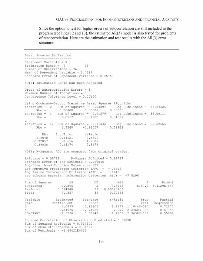
GAUSS PROGRAMMING FOR ECONOMETRICIANS AND FINANCIAL ANALYSTS
180
Since the option to test for higher orders of autocorrelation are still included in theprogram (see lines 12 and 13), the estimated AR(3) model is also tested for problemsof autocorrelation. Here are the estimation and test results with the AR(3) errorstructure:
Least Squares Estimation------------------------Dependent Variable = XEstimation Range = 4 39Number of Observations = 36Mean of Dependent Variable = 5.7319Standard Error of Dependent Variable = 0.45153
NOTE: Estimation Range Has Been Adjusted.
Order of Autoregressive Errors = 3Maximum Number of Iterations = 50Convergence Tolerance Level = 0.00100
Using Cochrane-Orcutt Iterative Least Squares AlgorithmIteration = 0 Sum of Squares = 0.03894 Log Likelihood = 71.84326
Rho = 0.00000 0.00000 0.00000Iteration = 1 Sum of Squares = 0.01579 Log Likelihood = 88.09111
Rho = 1.0537 -0.81992 0.31827…Iteration = 12 Sum of Squares = 0.01434 Log Likelihood = 89.82665
Rho = 1.3540 -0.92057 0.39938
Rho Std.Error t-Ratio1.3540 0.14121 9.5891
-0.92057 0.21656 -4.25080.39938 0.14174 2.8178
NOTE: R-Square, AOV are computed from original series.
R-Square = 0.99799 R-Square Adjusted = 0.99787Standard Error of the Estimate = 0.020845Log-Likelihood Function Value = 89.827Log Ammemiya Prediction Criterion (APC) = -7.6612Log Akaike Information Criterion (AIC) = -7.6616Log Schwarz Bayesian Information Criterion (BIC) = -7.5296
Sum of Squares SS DF MSS F Prob>FExplained 7.0896 2 3.5448 8157.7 3.4129E-045Residual 0.014340 33 0.00043453Total 7.1357 35 0.20388
Variable Estimated Standard t-Ratio Prob PartialName Coefficient Error 33 DF >|t| RegressionL 1.0433 0.11306 9.2277 1.1644E-010 0.72070K 0.54676 0.074920 7.2979 2.2460E-008 0.61743CONSTANT -2.5236 0.38943 -6.4802 2.3638E-007 0.55996
Squared Correlation of Observed and Predicted = 0.99800Sum of Squared Residuals = 0.014340Sum of Absolute Residuals = 0.56667Sum of Residuals = -1.68421E-012

AUTOCORRELATION
181
First-Order Rho = -0.0040825Durbin-Watson Test Statistic = 1.8661
Breusch-Godfrey LM Tests for AutocorrelationChi-Sq DF Prob>Chi-Sq
AR( 1) 0.41856 1 0.51766AR( 2) 0.86990 2 0.64730AR( 3) 3.3268 3 0.34393AR( 4) 3.4588 4 0.48416
Autocorrelation and Partial Autocorrelation FunctionsARMA Model SpecificationMean = 3.4232e-015 Standard Error = 0.020241
Lag AR S.E.(AR) PAR S.E.(PAR) Box-Pierce Ljung-Box1 -0.0039777 0.16667 -0.0039777 0.16667 0.00056961 0.000618432 -0.086337 0.16791 -0.086355 0.16667 0.26892 0.300543 -0.20318 0.17460 -0.20543 0.16667 1.7551 2.01194 -0.0027129 0.17460 -0.016352 0.16667 1.7554 2.01225 0.10710 0.17642 0.074897 0.16667 2.1683 2.51846 -0.18193 0.18156 -0.23380 0.16667 3.3599 4.02777 0.060756 0.18212 0.073555 0.16667 3.4928 4.20188 -0.14740 0.18540 -0.15926 0.16667 4.2749 5.26339 0.15411 0.18893 0.092475 0.16667 5.1299 6.466710 0.019960 0.18899 0.0049687 0.16667 5.1443 6.487611 -0.20234 0.19491 -0.24119 0.16667 6.6182 8.728112 -0.24101 0.20302 -0.28134 0.16667 8.7093 12.039
Based on the Breusch-Godfrey LM test up to the 4th order as well as the plot of the12-lag autocorrelation function and the associated Box-Pierce and Ljung-Box Q teststatistics, the estimated model with AR(3) error structure is now free ofautocorrelation. The estimated model is superior to that of correcting only for first-order autocorrelation.
In summary,
ln(X) = -2.52 + 1.04 ln(L) + 0.55 ln(K) + εs.e. (0.39) (0.11) (0.08)
ε = 1.35 ε-1 - 0.93 ε-2 + 0.40 ε-3s.e. (0.14) (0.22) (0.14)
Autoregressive and Moving Average Models: An IntroductionGPE can handle the estimation of a more complicated regression model involvingautoregressive and moving average autocorrelated errors. In addition to the p-th orderautoregressive structure AR(p) discussed earlier such as
ε i = ρ1ε i-1 + ρ2ε i-2 +…+ ρpε i-p + υi ,

GAUSS PROGRAMMING FOR ECONOMETRICIANS AND FINANCIAL ANALYSTS
182
the q-th order moving average error structure MA(q) is specified as
ε i = υi - θ1υ i-1 - θ2υ i-2 -…- θqυ i-q .
Or in combination with the autoregressive structure, that is ARMA(p,q) , we have
ε i = ρ1ε i-1 + ρ2ε i-2 +…+ ρpεi-p - θ1υ i-1 - θ2υ i-2 -…- θqυ i-q + υi
where the filtered error term υi is assumed to be normally independently distributed.Given a mixed error process of AR(p) and MA(q), or ARMA(p,q), the estimation ofthe p-element AR and q-element MA parameters is typically carried out by a nonlinearoptimization algorithm. To be more specific, nonlinear least squares or maximumlikelihood is called for in the estimation of an error structure with a moving averagecomponent. Without the moving average specification, the estimated autoregressiveparameters are computed by the methods described earlier in previous lessons.
With GPE, the following input control variables are relevant to the estimation of anerror structure with autoregressive and moving average components:
• _arma Autoregressive moving average orders• _nlopt Nonlinear least squares or maximum likelihood• _method Nonlinear optimization method• _iter Iteration limit• _conv Convergence criteria• _tol Convergence tolerance level
Among these control variables, only _arma is new. The other variables are related tononlinear model estimation discussed in Chapters VI and VII. The variable _arma isused to specify the orders of the autoregressive and moving average components ofthe error structure. It is a column vector consisting of at least two elements: the first isthe order of the autoregressive component, followed by the order of the movingaverage. For example,
_arma = 1,1;
specifies an error process of the first-order autoregressive and first-order movingaverage. A pure moving average of q-th order is set by _arma = 0,q.Obviously, _arma = p,0 is identical as _ar = p where p is the order numberof the autocorrelation. For parameter estimation, by providing the initial guess valuesof autoregressive and moving average parameters will be helpful for the convergence.These values could be appended to the variable _arma, in which the first twoelements are always the order of the respective process. We note that the estimatednonlinear ARMA error structure is conditional to data initialization for the beginning

AUTOCORRELATION
183
observations necessary to compute the process. For convenience, in GPE, we initializethe data series with the sample mean of model errors.
Lesson 10.6: ARMA(1,1) Error Structure
In normal situations, a higher order of autoregressive structure can be specified with alower order moving average structure, and vice versa. In order to keep the estimationsimple, we recommend the use of a lower order model. Of course, this is a matter oftaste and also depends on the theory and computational experience. Earlier lessons onestimating the U.S. production function suggest that the model is better described withan AR(3) error structure (see Lesson 10.5). An alternative would be to estimate theerror process using a MA(1) structure or a mixed structure of autoregressive andmoving average at a lower order, say, ARMA(1,1). Lesson 10.6 demonstrates theestimation of an ARMA(1,1) model.
123
4567
8
910111213
141516171819
/*** Lesson 10.6: ARMA(1,1) Error Structure*/use gpe2;output file = gpe\output10.6 reset;load data[40,6]= gpe\cjx.txt;
year = data[2:40,1];X = ln(data[2:40,2]);L = ln(data[2:40,3]);K = ln(data[2:40,5]);
call reset;
_names = "X","L","K";_rstat = 1;_rplot = 2;_bgtest = 4;_acf = 12;
_arma = 1,1; @ ARMA(1,1) error structure @_nlopt = 1; @ maximum likelihood estimation @_method = 5; @ QHC optimization method @_iter = 50; @ 50 iterations @call estimate(X,L~K);end;
To double check for autocorrelation after the specification of ARMA(1,1) isestimated, we keep _bgtest and _acf (lines 12 and 13) in the program.
The ARMA(1,1) structure is estimated with the nonlinear maximum likelihoodmethod using Quadratic Hill Climbing algorithm. It took 34 iterations to achieve theconvergence. Here is the abridged regression output of the estimated Cobb-Douglasproduction function with an ARMA(1,1) error structure:

GAUSS PROGRAMMING FOR ECONOMETRICIANS AND FINANCIAL ANALYSTS
184
Least Squares Estimation------------------------Dependent Variable = XEstimation Range = 1 39Number of Observations = 39Mean of Dependent Variable = 5.6874Standard Error of Dependent Variable = 0.46096
Maximum Likelihood Estimation for Nonlinear Error StructureARMA(1 ,1 ) Autoregressive Moving Average Process
Maximum Number of Iterations = 50Step Size Search Method = 0Convergence Criterion = 0Tolerance = 0.001
Initial Result:Sum of Squares = 0.043221Log Likelihood = 77.359Parameters = 1.4508 0.38381 -3.9377 0.00000 0.00000
Using Quadratic Hill-Climbing AlgorithmIteration = 1 Step Size = 2.3579 Log Likelihood = 89.926Parameters = 1.4410 0.38615 -3.8967 0.45558 -0.46020Iteration = 34 Step Size = 1.0000 Log Likelihood = 93.016Parameters = 1.1051 0.54833 -2.8796 0.62424 -0.67141
Final Result:Iterations = 34 Evaluations = 50154Sum of Squares = 0.019363Log Likelihood = 93.016Parameters = 1.1051 0.54833 -2.8796 0.62424 -0.67141Gradient of Log Likelihood = 0.022545 0.019469 0.0044089 -0.00020935 0.00015670
Parameter Std.Error t-RatioAR(1 ) 0.62424 0.22900 2.7259MA(1 ) -0.67141 0.17318 -3.8770
NOTE: R-Square, AOV are computed from original series.
R-Square = 0.99760 R-Square Adjusted = 0.99747Standard Error of the Estimate = 0.022282Log-Likelihood = 93.016Log Ammemiya Prediction Criterion (APC) = -7.4538Log Akaike Information Criterion (AIC) = -7.4541Log Schwarz Bayesian Information Criterion (BIC) = -7.3261
Sum of Squares SS DF MSS F Prob>FExplained 8.0216 2 4.0108 7456.8 7.4158E-048Residual 0.019363 36 0.00053787Total 8.0744 38 0.21248
Variable Estimated Standard t-Ratio Prob PartialName Coefficient Error 39 DF >|t| RegressionL 1.1051 0.16031 6.8934 3.0026E-008 0.54923K 0.54833 0.083877 6.5373 9.3096E-008 0.52285CONSTANT -2.8796 0.54958 -5.2397 5.8625E-006 0.41314

AUTOCORRELATION
185
Squared Correlation of Observed and Predicted = 0.99761Sum of Squared Residuals = 0.019363Sum of Absolute Residuals = 0.67628Sum of Residuals = 1.84261E-002First-Order Rho = -0.0028812Durbin-Watson Test Statistic = 1.9895
Breusch-Godfrey LM Tests for AutocorrelationChi-Sq DF Prob>Chi-Sq
AR( 1) 0.50222 1 0.47852AR( 2) 0.86082 2 0.65024AR( 3) 5.3236 3 0.14958AR( 4) 5.4880 4 0.24079
Autocorrelation and Partial Autocorrelation FunctionsARMA Model SpecificationMean = 0.00047246 Standard Error = 0.022568
Lag AR S.E.(AR) PAR S.E.(PAR) Box-Pierce Ljung-Box1 -0.0037201 0.16013 -0.0037201 0.16013 0.00053974 0.000582352 -0.049522 0.16052 -0.049537 0.16013 0.096186 0.106573 -0.23055 0.16880 -0.23150 0.16013 2.1691 2.46744 0.064036 0.16942 0.060518 0.16013 2.3290 2.65475 0.24181 0.17805 0.23366 0.16013 4.6095 5.40476 -0.13491 0.18065 -0.20050 0.16013 5.3193 6.28657 0.032581 0.18080 0.086890 0.16013 5.3607 6.33968 -0.26120 0.19023 -0.18931 0.16013 8.0215 9.85879 0.18387 0.19474 0.11395 0.16013 9.3400 11.66110 0.0024843 0.19474 -0.030052 0.16013 9.3403 11.66111 -0.10407 0.19616 -0.16014 0.16013 9.7627 12.28012 -0.13637 0.19857 -0.093640 0.16013 10.488 13.381
If you prefer to use nonlinear least squares instead of maximum likelihood toestimate the ARMA model, just delete line 15 or change it to:
_nlopt = 0;
The result should be the same. Why?
Summarizing, the estimated model with ARMA(1,1) error structure is:
ln(X) = -2.88 + 1.11 ln(L) + 0.55 ln(K) + εs.e. (0.55) (0.16) (0.08)
ε = 0.62 ε-1 - 0.67 υ-1s.e. (0.23) (0.17)
Both the parameter estimates of AR(1) and MA(1) are statistically significant anduseful for correcting autocorrelation. Based on the Breusch-Godfrey LM test up to the4th-order, as well as the 12-lag autocorrelation function plot and the associated Box-Pierce and Ljung-Box Q test statistics, the estimated ARMA(1,1) model is as good as

GAUSS PROGRAMMING FOR ECONOMETRICIANS AND FINANCIAL ANALYSTS
186
that of the AR(3) specification presented in the Lesson 10.5. Both models areessentially equivalent.
Nonlinear Maximum Likelihood EstimationIt is clear that a regression model with autocorrelation is intrinsically a nonlinearmodel. Even with the basic linear regression equation, ε = Y – Xβ, the functional formof model error for estimation is nonlinear in the parameters. Consider the AR(1),MA(1), and ARMA(1,1):
Residual Residual FunctionAR(1) υi = εi – ρ εi-1 (Yi – ρYi-1) – (Xi – ρXi-1)βMA(1) υi = εi + θ υi-1 (Yi – Xiβ) + θ υi-1ARMA(1,1) υi = εi – ρ εi-1 + θ υi-1 (Yi – ρYi-1) – (Xi – ρXi-1)β + θ υi-1
The nonlinearity of AR(1) is clearly due to the product of parameters β and ρ, whileMA(1) is recursively weighted by θ. ARMA(1,1) is a mixed process of AR(1) andMA(1), and therefore contains both of aforementioned nonlinearities. For modelestimation, the beginning observation of data series may be lost if not properlyinitialized. The built-in ARMA estimation of GPE is conditional to the simple datainitialization with the sample mean. We have seen the Prais-Winston transformationfor the first observation of AR(1): 1-ρ2 Y1 and 1-ρ2 X1. This adds more nonlinearcomplexity into the model and makes maximum likelihood the preferred method forestimation.
Given N sample data observations of Z = [Y,X], the concentrated log-likelihoodfunction for the AR(1) model is
ll*(β,ρ) = -N/2 (1+2π-ln(N)) –N/2 ln(υ’υ) + ln(1-ρ2)
For MA(1), the recursive process starts with the initial residual υ0 which is typicallyset to its expected value (i.e., zero) or the sample mean. An alternative is to estimateυ0 directly. The concentrated log-likelihood function is simpler but conditional to theinitialization of υ0 as follows:
ll*(β,θ,υ0) = -N/2 (1+2π-ln(N)) –N/2 ln(υ’υ)
The concentrated log-likelihood function of the mixed process ARMA(1,1) is similarto that of AR(1) in which the residual function depends on both ρ and θ (in addition toβ) and subject to the initialization of υ0 and transformation for the first dataobservation.

AUTOCORRELATION
187
Lesson 10.7: Nonlinear ARMA Model Estimation
We continue with the previous example of U. S. Cobb-Douglas production functionand estimate the three autoregressive error structures: AR(1), MA(1), andARMA(1,1). Using the method of nonlinear maximum likelihood, the regressionparameter β and autoregressive coefficients ρ and/or θ are estimated jointly. ForMA(1) and ARMA(1,1), the initialization of residuals with zero expected value isapplied. As we have mentioned earlier, the nonlinear method may produce differentresults compared with the linear iterative approximations as employed in theCochrane-Orcutt approach (Lesson 10.3) or the GPE built-in method of conditionalnonlinear maximum likelihood (Lesson 10.6). However, the results are not drasticallydifferent.
This lesson differs from the previous ones in that the program setup is for nonlinearmaximum likelihood estimation. Nonlinear maximum likelihood was covered inChapter VII, and it is helpful to go back for a thorough review of the estimationtechnique.
For each of three autoregressive models, the residual function must be defined inorder to maximize the objective log-likelihood function. The block from line 34 toline 41 defines the residual function for an AR(1) model. The MA(1) specification isgiven in lines 42 through 48, while the ARMA(1,1) is specified from line 49 to line57. Notice that AR(1) and ARMA(1,1) require the use of Jacobians in the likelihoodfunction. The Jacobian function is defined in the block from line 29 to line 33.
123
45678
9
1011121314
151617
/*** Lesson 10.7: Maximum Likelihood Estimation** AR(1), MA(1), ARMA(1,1)*/use gpe2;output file = gpe\output10.7 reset;load data[40,6]= gpe\cjx.txt;
year = data[2:40,1];X = ln(data[2:40,2]);L = ln(data[2:40,3]);K = ln(data[2:40,5]);data=X~L~K;
@ OLS estimates as initial values @b=data[.,1]/(ones(rows(data),1)~data[.,2:3]);
call reset;_nlopt=1;_method=0;_iter=100;_conv=1;
_b=b|0.5;_jacob=&jcb;_names = "CONSTANT","LN(L)","LN(K)","AR(1)";

GAUSS PROGRAMMING FOR ECONOMETRICIANS AND FINANCIAL ANALYSTS
188
18
19202122
23242526
27
282930313233
3435363738
394041
4243444546
4748
4950515253
54555657
call estimate(&ar,data);
_b=b|0;_jacob=0;_names = "CONSTANT","LN(L)","LN(K)","MA(1)";call estimate(&ma,data);
_b=b|0.5|0;_jacob=&jcb;_names = "CONSTANT","LN(L)","LN(K)","AR(1)","MA(1)";call estimate(&arma,data);
end;
proc jcb(x,b); @ jacobian for AR(1) and ARMA(1,1) @local j;j=ones(rows(x),1);j[1]=sqrt(1-b[4]^2);retp(j);
endp;
proc ar(x,b);local n,e,u;n=rows(x);e=x[.,1]-b[1]-b[2]*x[.,2]-b[3]*x[.,3];u=e-b[4]*lagn(e,1);@ first obs transformation @u[1]=sqrt(1-b[4]^2)*e[1];retp(u);
endp;
proc ma(x,b);local n,e,u;n=rows(x);e=x[.,1]-b[1]-b[2]*x[.,2]-b[3]*x[.,3];u=recserar(e,e[1],b[4]); @ u[1]=e[1] since u[0]=0 @
/*@ recursive computation of errors using @@ built-in RECSERAR is the same as below: @u=e; @ initialize: u[1]=e[1] @i=2;do until i>n;
u[i]=e[i]+b[4]*u[i-1];i=i+1;
endo;*/
retp(u);endp;
proc arma(x,b);local n,e,u,v;n=rows(x);e=x[.,1]-b[1]-b[2]*x[.,2]-b[3]*x[.,3];u=e-b[4]*lagn(e,1);@ first obs transformation @u[1]=sqrt(1-b[4]^2)*e[1];v=recserar(u,u[1],b[5]);retp(v);
endp;

AUTOCORRELATION
189
Using the linear least squares estimates as initial values of parameters (line 9), lines15-18 carry out the estimation for the AR(1) model. Here is the result:
Maximum Likelihood Estimation-----------------------------Number of Observations = 39Number of Parameters = 4
Maximum Number of Iterations = 100Step Size Search Method = 0Convergence Criterion = 1Tolerance = 0.001
Initial Result:Sum of Squares = 0.029940Log Likelihood = 84.518Parameters = -3.9377 1.4508 0.38381 0.50000
Using Berndt-Hall-Hall-Hausman (BHHH) Algorithm
Final Result:Iterations = 17 Evaluations = 4914Sum of Squares = 0.027133Log Likelihood = 86.438Gradient of Log Likelihood = 4.9312e-005 0.00023054 0.00020964 2.6217e-005
AsymptoticParameter Std. Error t-Ratio
CONSTANT -2.8220 0.56933 -4.9567LN(L) 1.0926 0.17753 6.1546LN(K) 0.54995 0.096866 5.6775AR(1) 0.77832 0.13059 5.9599
The BHHH method is used for log-likelihood function maximization (see line 12), andit converges in 17 iterations. As seen in line 15, the initial value of the AR(1)coefficient is set to 0.5. The solution is close to that of Cochrane-Orcutt (Lesson 10.3)and Hildreth-Lu (Lesson 10.4) procedures. The crucial point of this model is the useof first observation transformation (line 39) and the resulting Jacobian function mustbe incorporated for the exact maximum likelihood estimation.
Similarly, the MA(1) model is estimated in lines19-22 with the starting value of theMA(1) coefficient at 0. Here is the estimation result:
Maximum Likelihood Estimation-----------------------------Number of Observations = 39Number of Parameters = 4
Maximum Number of Iterations = 100

GAUSS PROGRAMMING FOR ECONOMETRICIANS AND FINANCIAL ANALYSTS
190
Step Size Search Method = 0Convergence Criterion = 1Tolerance = 0.001
Initial Result:Sum of Squares = 0.043382Log Likelihood = 77.286Parameters = -3.9377 1.4508 0.38381 0.00000
Using Berndt-Hall-Hall-Hausman (BHHH) Algorithm
Final Result:Iterations = 29 Evaluations = 8073Sum of Squares = 0.022342Log Likelihood = 90.226Gradient of Log Likelihood = -0.00016182 -0.00094511 -0.00082061 4.1086e-005
AsymptoticParameter Std. Error t-Ratio
CONSTANT -3.6176 0.27477 -13.166LN(L) 1.3379 0.094876 14.102LN(K) 0.44264 0.054316 8.1495MA(1) -0.81620 0.095539 -8.5431
As the MA(1) model does not use the first-observation transformation of AR(1), theJacobian function should not be called (see line 20). The residual function is definedwith an autoregressive recursive series using GAUSS built-in function RECSERAR(line 46). The initialization of the recursive series is the expected value of the series,which is zero. Line 46 shows the use of RECSERAR with initialization. Check theGAUSS manual or online help for more information about the procedureRECSERAR. The computation of autoregressive recursive series is also explained inthe comment block immediately below line 46.
Conditional to the initialization of the recursive moving average series
υi = (Yi – Xiβ) + θ υi-1
we have obtained the maximum likelihood estimates of β and θ as shown above. Fori = 1, υ0 = 0 is assumed. The alternative is to estimate υ0 together with β and θ.Simply replace line 46 with the following:
u=recserar(e,e[1]+b[5]*b[4],b[4]);
where b[5] is the unknown υ0 to be estimated with the rest of the parameters.Starting from the initial guess of (θ,υ0) at (0,0), in addition to the linear least squaresestimator of β, the model is estimated exactly the same way as before except that line19 should be:
_b=b|0|0;

AUTOCORRELATION
191
How the estimation results differ from those of Lesson 10.7, which assumed υ0 = 0?We leave this question to you.
For ARMA(1,1), both the first observation transformation of AR(1) andautoregressive recursive series with initialization of MA(1) are required. The model isestimated in lines 23-26. Here is the estimation result:
Maximum Likelihood Estimation-----------------------------Number of Observations = 39Number of Parameters = 5
Maximum Number of Iterations = 100Step Size Search Method = 0Convergence Criterion = 1Tolerance = 0.001
Initial Result:Sum of Squares = 0.029940Log Likelihood = 84.518Parameters = -3.9377 1.4508 0.38381 0.50000 0.00000
Using Berndt-Hall-Hall-Hausman (BHHH) Algorithm
Final Result:Iterations = 21 Evaluations = 7059Sum of Squares = 0.018525Log Likelihood = 93.879Gradient of Log Likelihood = -0.00012631 -0.00065739 -0.000554470.00015394 -1.6021e-006
AsymptoticParameter Std. Error t-Ratio
CONSTANT -2.6041 0.42941 -6.0644LN(L) 1.0321 0.12537 8.2320LN(K) 0.57271 0.071019 8.0641AR(1) 0.66145 0.14519 4.5559MA(1) -0.71077 0.12402 -5.7309
Again, for estimating the above ARMA(1,1) model:
υi = (Yi – ρYi-1) – (Xi – ρXi-1)β + θ υi-1
υ0 = 0 is assumed for i = 1. The alternative is to estimate υ0 together with β, ρ, andθ. Simply replace line 55 with the following:
v=recserar(u,u[1]+b[6]*b[5],b[5]);
where b[6] is the unknown υ0 to be estimated with the rest of the parameters.Starting from the initial guess of (ρ,θ,υ0) at (0.5,0,0), in addition to the linear leastsquares estimator of β, the model is estimated exactly the same way as before except

GAUSS PROGRAMMING FOR ECONOMETRICIANS AND FINANCIAL ANALYSTS
192
that line 23 should be changed to:
_b=b|0.5|0|0;
To summarize the discussion of autoregressive regression models, we put together andcompare the estimation results of the U. S. Cobb-Douglas production function:
ln(X) = β0 + β1 ln(L) + β2 ln(K) + ε
Where X is output, and the two factor inputs are labor L and capital K. The followingtable presents the parameter estimates (numbers in parentheses are the estimatedstandard errors of the parameters) and the corresponding log-likelihood function valuell for each model.
(1)Lesson
10.1
(2)Lesson
10.3
(3)Lesson
10.4
(4)Lesson
10.7
(5)Lesson
10.7
(6)Lesson
10.7
(7)Lesson
10.6β1 1.451
(0.083)1.068
(0.151)1.050
(0.153)1.093
(0.178)1.338
(0.095)1.032
(0.125)1.105
(0.160)β2 0.384
(0.048)0.558
(0.096)0.563
(0.098)0.550
(0.097)0.443
(0.054)0.573
(0.071)0.548
(0.084)β0 -3.94
(0.237)-2.73
(0.456)-2.66
(0.465)-2.82
(0.569)-3.62
(0.275)-2.60
(0.429)-2.88
(0.550)ρ 0 0.805
(0.096)0.826
(0.090)0.778
(0.131)0 0.661
(0.145)0.624
(0.229)θ 0 0 0 0 -0.816
(0.096)-0.711
(0.124)-0.671
(0.173)ll 77.286 86.420 86.379 86.438 90.226 93.879 93.016
The top row of the table identifies the model and its corresponding lesson: (1) Lesson10.1 is the ordinary least squares estimates without autocorrelation correction; (2)Lesson 10.3 is AR(1) model using the Cochrane-Orcutt iterative procedure; (3)Lesson 10.4 is the same AR(1) model using Hildreth-Lu grid search method; (4), (5),and (6) are based on Lesson 10.7 using nonlinear maximum likelihood estimation forthe model AR(1), MA(1), and ARMA(1,1) respectively. The last column (7) is theARMA(1,1) model estimated with the GPE built-in conditional maximum likelihoodmethod in Lesson 10.6. All the methods use the entire sample of 39 observations from1929 to 1967. For model comparison, the statistics of pair-wise Likelihood Ratio (LR)will be useful. It is immediately clear that the model must be corrected forautocorrelation. The plain OLS model (1) is rejected based on LR tests with all theother models. Finally, The structure of autoregressive moving average ARMA(1,1) ofboth Lessons 10.6 and 10.7 can not be rejected.

XIDistributed Lag Models
With the proper use of distributed lags, regression models can be expanded to includedynamic features such as long-run and short-run elasticities and multipliers foranalysis. In this chapter we will consider two popular setups of distributed lags:geometric, or Koyck lags, and polynomial, or Almon lags. The former is an infinitedistributed lags model with a geometric declining pattern, which in turn can betransformed into a lagged dependent variable model. The latter is a finite distributedlags model with polynomial functional restrictions. The combination of the two is theso-called Autoregressive Distributed Lag model.
Lagged Dependent Variable ModelsApplications of lagged dependent variable models include partial adjustment andadaptive expectation estimations. These models relate the long-run and short-runbehavior of influential variables. However, regression models with lagged dependentvariables may possess some undesirable characteristics. Possible problems includecorrelated error terms and random regressors. The resulting least squares estimation isbiased, inconsistent, and inefficient. The lagged dependent variable model isconsidered in Lesson 11.1.
For estimating such a model with lagged dependent variables, Instrumental VariableEstimation (IV) is suggested. IV weighs the trade-off between “biasedness” and“inefficiency” and obtains a “consistent” parameter estimator which minimizes the illeffects of using lagged dependent variables. Instrumental variable estimation for alagged dependent variable model is the focus of Lesson 11.2.
Lesson 11.1: Testing for Autocorrelation with Lagged Dependent Variable
A classical consumption-income relationship based on the Permanent IncomeHypothesis is a good example to demonstrate the construction, testing, and estimationof the lagged dependent variable model:
C = β0 + β1Y + β2 C-1 + ε

GAUSS PROGRAMMING FOR ECONOMETRICIANS AND FINANCIAL ANALYSTS
194
where C is consumption and Y is income. Assuming a simple partial adjustment ofshort-run consumption towards its long-run equilibrium, the lagged dependentvariable C-1 is included in the model specification.
To estimate the above consumption-income equation, we introduce a new data fileusyc87.txt. This data file consists of three variables: YEAR, Y, and C. YEAR is justthe time indicator ranging from 1929 to1994. Y is personal disposable income, and Cis personal consumption expenditure. Both income and consumption time series areexpressed in billions of 1987 dollars. In total there are 66 observations.
In this lesson we will estimate a lagged dependent variable model. The only new inputcontrol variable is _dlags which is used to specify the number of lags desired. Forexample, by setting _dlags = 1, GPE inserts the first lag of the dependent variableinto the regression equation for least squares estimation. The lagged dependentvariable is added in front of the other explanatory variables. The Durbin-H TestStatistic is automatically included in the output of _rstat when _dlags is set to avalue greater than zero.
12345
678910
11121314
/*** Lesson 11.1: Lagged Dependent Variable Model** Estimation and Testing for Autocorrelation*/use gpe2;output file = gpe\output11.1 reset;load z[67,3] = gpe\usyc87.txt;y = z[2:67,2];c = z[2:67,3];
call reset;_names = "c","y";_rstat = 1;_dlags = 1;call estimate(c,y);
_ar = 1;_iter = 50;call estimate(c,y);end;
If more than one lag is needed, just change the value of _dlags to the desiredpositive number of lags.
To estimate the model is simple, but to evaluate and interpret the effect of a laggeddependent variables is not. Line 9 specifies that the model to be estimated includes thefirst lag of the dependent variable. The following call to estimate (line 10)proceeds to carry out least squares estimation of the model. Since _rstat is set to 1in line 8, a summary of residual statistics including the new Durbin-H test statistic ispresented.

DISTRIBUTED LAG MODELS
195
Alternatively, you can create the lagged dependent variable and then include it inestimate as an independent variable. In GAUSS, the lagged variable isconstructed with the command lag1 or lagn. This method requires the extra stepof handling the initial observation lost from lagging the dependent variable explicitlyso that the program will run. Setting the GPE control variable _begin to thebeginning of the usable sample for estimation may be necessary. In addition, GPEwill not treat the variable you created differently from the rest of the explanatoryvariables. Therefore, the Durbin-H test statistic, unique to the lagged dependentvariable model, is not computed. In passing, we note that testing linear restrictionsinvolving lagged dependent variables requires specifying restrictions on thosevariables explicitly.
The result of the first least squares estimation (line 10) is given below:
Least Squares Estimation------------------------Dependent Variable = CEstimation Range = 2 66Number of Observations = 65Mean of Dependent Variable = 1588.2Standard Error of Dependent Variable = 955.14
NOTE: Estimation Range Has Been Adjusted.Lagged Dependent Variables Used = 1
R-Square = 0.99927 R-Square Adjusted = 0.99925Standard Error of the Estimate = 26.154Log-Likelihood Function Value = -302.86Log Ammemiya Prediction Criterion (APC) = 6.5731Log Akaike Information Criterion (AIC) = 6.5731Log Schwarz Bayesian Information Criterion (BIC) = 6.6734
Sum of Squares SS DF MSS F Prob>FExplained 5.8344E+007 2 2.9172E+007 42648. 4.9624E-098Residual 42410. 62 684.03Total 5.8387E+007 64 9.1229E+005
Variable Estimated Standard t-Ratio Prob PartialName Coefficient Error 62 DF >|t| RegressionC-1 0.69465 0.057390 12.104 5.6098E-018 0.70265Y 0.29660 0.051205 5.7925 2.4894E-007 0.35114CONSTANT -0.56350 6.4092 -0.087920 0.93022 0.00012466
Squared Correlation of Observed and Predicted = 0.99927Sum of Squared Residuals = 42410.Sum of Absolute Residuals = 1274.2Sum of Residuals = -1.12485E-008First-Order Rho = 0.45221Durbin-Watson Test Statistic = 1.0769Durbin-H Statistic = 4.1974

GAUSS PROGRAMMING FOR ECONOMETRICIANS AND FINANCIAL ANALYSTS
196
Notice that the estimation range given in the first block of the output is from 2 to 66,using 65 observations. This is because the use of the first lag of the dependent variableon the right-hand-side of the regression equation. Next is a statement giving thenumber of lags included in the estimation.
The last line of the first block of output is the Durbin-H Statistic. Given the first-orderrho at 0.45 with the Durbin-H test statistic as high as 4.2 (comparing with the criticalvalues of a standardized normal distribution), the problem of autocorrelation is readilyapparent. Methods of correction for autocorrelation discussed in the previous chaptershould be used to improve the results of model estimation.
Lines 11 to 13 of the program correct and then re-estimate the model with a first orderautocorrelated error structure. The default Cochrane-Orcutt iterative method is used.We refer to the output file output11.1 for details of the regression results. Insummary, here is our estimated lagged dependent variable model with AR(1) errorstructure:
C = -6.284 + 0.487 Y + 0.484 C-1 + εs.e. (14.61) (0.065) (0.073)
ε = 0.648 ε-1s.e. (0.098)
The correction for first-order autocorrelation is certainly a right step to improve themodel. It may not be a bad idea to continue to carry out testing for higher orders ofautocorrelation. Remember to use the following statements before the last call ofestimate in the above program:
_bgtest = 4;_acf = 12;
With the results not shown here, we did not find a significant autocorrelationproblem at higher orders.
Lesson 11.2: Instrumental Variable Estimation
The more serious specification problem related to the lagged dependent variablemodel is random regressors. In Lesson 11.1, although the problem of autocorrelationseems easy to resolve by correcting the first order serial correlation, the estimatedparameters are still biased and inefficient. These problems are due to the ill effects ofrandom regressors that may be involved through the use of lagged dependentvariables.
To handle a lagged dependent variable model estimation with instrumental variables,GPE implements an estimation technique which uses the current and lagged

DISTRIBUTED LAG MODELS
197
explanatory variables as instruments for the lagged dependent variable. If longer lagsof the dependent variable are adopted or an autocorrelated error structure is identified,the instrumental variable estimation procedure may need to include more lags of theexplanatory variables as well. In the context of a lagged dependent variable model,instrumental variable estimation is activated by setting the following input controlvariable:
_ivar = 1;
The alternative is to specify the entire data matrix for the variable _ivar. This isuseful for applying instrumental variable estimation in other contexts such asmeasurement error in the regression model. We note that the matrix specification of_ivar requires that its size (rows and columns) to be at least as large as that of thedata matrix of explanatory variables.
We continue on from the end of Lesson 11.1, adding the option to estimate the modelusing instrumental variables in the following program:
12
345
6789101112
131415
/*** Lesson 11.2: Lagged Dependent Variable Model** Instrumental Variable Estimation*/use gpe2;output file=gpe\output11.2 reset;
load z[67,3]=gpe\usyc87.txt;y=z[2:67,2];c=z[2:67,3];
call reset;_names="c","y";_rstat=1;_dlags=1;_ar=1;_iter=50;call estimate(c,y);
_ivar=1;call estimate(c,y);end;
The only new addition to the program is Line 13:
_ivar = 1;
which calls for the use of internal instrumental variables GPE will construct for thelagged dependent variables. In addition, the autocorrelation correction is requested forthe first order (line 10), hence one additional lag of explanatory variables is needed aspart of the instrumental variables.

GAUSS PROGRAMMING FOR ECONOMETRICIANS AND FINANCIAL ANALYSTS
198
Alternatively, line 13 can be replaced with the explicitly defined instrumentalvariables as follows:
_ivar = y~lagn(y,1)~lagn(y,2)~ones(rows(y),1);_begin = 3;
The advantage is that you have more control over the addition of relevantinstrumental variables in order to improve the small-sample properties of theestimator. In contexts other than the lagged dependent variable model, instrumentalvariable estimation may be requested with the variable _ivar explicitly assigned toa data matrix no smaller than that of explanatory variables.
We note that the scalar definition of _ivar = 1 will only work when specifying apositive number of _dlags. _ivar = 1 without _dlags (or _dlags = 0)will result in a program error.
Looking at the output file output11.2, the results of the first regression in thislesson are the same as the results of the second regression of Lesson 11.1. The secondestimation of this lesson performs instrumental variable estimation while at the sametime correcting for first order serial correlation. We will show you only the partialresult of the second regression estimation:
Least Squares Estimation------------------------Dependent Variable = CEstimation Range = 3 66Number of Observations = 64Mean of Dependent Variable = 1604.9Standard Error of Dependent Variable = 953.09
NOTE: Estimation Range Has Been Adjusted.NOTE: Lagged Dependent Variables Used = 1NOTE: Instrumental Variables Used = 4
Order of Autoregressive Errors = 1Maximum Number of Iterations = 50Convergence Tolerance Level = 0.00100
Using Cochrane-Orcutt Iterative Least Squares AlgorithmIteration = 0 Sum of Squares = 50104.92594 Log Likelihood = -304.02779
Rho = 0.00000Iteration = 1 Sum of Squares = 31093.47963 Log Likelihood = -289.01518
Rho = 0.63232…Iteration = 8 Sum of Squares = 31055.04449 Log Likelihood = -289.01591
Rho = 0.66806
Rho Std.Error t-Ratio0.66806 0.097245 6.8699

DISTRIBUTED LAG MODELS
199
NOTE: R-Square, AOV are computed from original series.
R-Square = 0.99946 R-Square Adjusted = 0.99944Standard Error of the Estimate = 22.563Log-Likelihood = -289.02Log Ammemiya Prediction Criterion (APC) = 6.2785Log Akaike Information Criterion (AIC) = 6.2784Log Schwarz Bayesian Information Criterion (BIC) = 6.3796
Sum of Squares SS DF MSS F Prob>FExplained 5.7131E+007 2 2.8566E+007 56110. 2.6192E-100Residual 31055. 61 509.10Total 5.7228E+007 63 9.0838E+005
Variable Estimated Standard t-Ratio Prob PartialName Coefficient Error 61 DF >|t| RegressionC-1 0.45966 0.094109 4.8843 7.8449E-006 0.28114Y 0.50728 0.084052 6.0353 1.0194E-007 0.37388CONSTANT -3.8035 16.185 -0.23501 0.81499 0.00090457
Squared Correlation of Observed and Predicted = 0.99946Sum of Squared Residuals = 31055.Sum of Absolute Residuals = 1040.2Sum of Residuals = -1.67559E+001First-Order Rho = 0.20383Durbin-Watson Test Statistic = 1.5864Durbin-H Statistic = 2.5137
Because instrumental variables are used essentially to replace lagged dependentvariables in the model estimation, testing and correction for autocorrelation is nowthe same as in the classical model. The Durbin-Watson test statistic can be applied asusual.
The model uses four instrumental variables: the original, first and second lags ofexplanatory independent variable Y, and the constant term. The second lag is includeddue to the first-order serial correlation being specified for model estimation.
Comparing the estimation results from not using instrumental variables,
C = -6.284 + 0.487 Y + 0.484 C-1 + εs.e. (14.61) (0.065) (0.073)
ε = 0.648 ε-1s.e. (0.098)
with our estimated model using instrumental variables

GAUSS PROGRAMMING FOR ECONOMETRICIANS AND FINANCIAL ANALYSTS
200
C = -3.804 + 0.507 Y + 0.460 C-1 + εs.e. (16.185) (0.084) (0.094)
ε = 0.668 ε-1s.e. (0.097)
we see that their parameter estimates are similar. But the current estimated standarderrors of the parameters are slightly larger than the standard errors resulting from notusing the instrumental variables. Nevertheless, the conclusions of statistical inferencesare not effected in this example.
We will keep the interpretation of the estimated model using instrumental variablesbrief. First, the short-run marginal propensity to consume is 0.51. With the estimatedcoefficient 0.46 for the lagged dependent variable, the long-run consumption changeis about 0.94 for each dollar increase of income. To realize 50% of the total effect(that is, half of 0.94 or 0.47) will take 0.89 years. This is the concept of median lagfrequently used in dynamic analysis. The other measurement is the lag-weightedaverage or the mean lag, which is computed at about 0.85 years.
Remember the formula for computing the median lag and mean lag? Let λ be theestimated parameter of the lagged dependent variable. Then the median lag is
computed as ln(0.5) ln(λ) , and the mean lag is
λ1-λ .
Polynomial Lag ModelsBy imposing polynomial functional restrictions on the finite distributed lags of someor all explanatory variables, the dynamic model can be estimated with traditionalrestricted least squares methodology. In this model we specify the polynomialdistributed lag structure for each explanatory variable. Given the number ofdistributed lags q, a polynomial function of order p is used to describe p-1 number ofturning points in the lag structure. In addition, we can add end-point restrictions to “tiedown” the effects of distributed lags at either or both ends. For a polynomial lagmodel to be meaningful, p must be greater than 1, and the total number of lags (q)must be greater than the polynomial orders (p). If q equals p, the distributed lag modelis without polynomial restrictions.
In GPE, a polynomial lag model is defined with the input control variable _pdl. Thevariable _pdl is a 3-column matrix with the number of the rows corresponding to thenumber of explanatory variables. A polynomial lag structure must be defined for eachvariable (row) in the _pdl matrix. The 3-column entry for each explanatory variablemust be separately called out for the lags q, polynomial orders p, and end-pointrestrictions r in that order. End-point restrictions “tie down” one or both ends of the

DISTRIBUTED LAG MODELS
201
polynomial’s curve, enforcing a theoretical or empirical justification of the lagstructure. For variables that do not have the polynomial lag structure, the 3-columnentry: 0 0 0 should be used. Normally the constant term is not included in the _pdlmatrix, unless otherwise specified.
Estimating a model with a polynomial lag structure defined for each explanatoryvariable is essentially the same as restricted least squares. The number of restrictionsis (q-p) polynomial restrictions plus the number of end-point restrictions. Anyadditional linear restrictions imposed with the variable _restr must take intoaccount the correct structure of right-hand-side variables that _pdl may add to theoriginal equation.
Lesson 11.3: Almon Lag Model Revisited
In this lesson, we will revisit the relationship between appropriations (CAPP) andcapital expenditure (CEXP) first introduced in Lesson 4.1. The data file is almon.txtin which the quarterly data series, CEXP and CAPP from 1953 to 1967 are provided.In the following, we try to duplicate the original study of S. Almon published in 1965.Almon’s regressions were computed using a fourth-order polynomial and lagsextending in seven periods. She also included seasonal dummy variables whose fourcoefficients were constrained to sum to zero. Also, both end-points are restricted onthe polynomial lags.
Here is the program:
123
456
78910
111213
14151617
/*** Lesson 11.3: Polynomial Distributed Lag Model** Almon Lag Model Revisited*/use gpe2;output file = gpe\output11.3 reset;load almon[61,3] = gpe\almon.txt;
cexp = almon[2:61,2];capp = almon[2:61,3];qt = almon[2:61,1];
q1=(qt%10).==1; @ quarterly seasonal dummies @q2=(qt%10).==2;q3=(qt%10).==3;q4=(qt%10).==4;
call reset;_rstat = 1;_end = 36;
/* restrictions on all dummy variables */_const = 0;_restr = 0 0 0 0 0 0 0 0 1 1 1 1 0;_pdl = 7 4 2,
0 0 0,

GAUSS PROGRAMMING FOR ECONOMETRICIANS AND FINANCIAL ANALYSTS
202
181920212223
0 0 0,0 0 0,0 0 0;
_names="cexp","capp","q1","q2","q3","q4";call estimate(cexp,capp~q1~q2~q3~q4);end;
In her original discussion Almon used only 36 observations, therefore we end ourestimation at 36 (line 13). As you will remember, suppressing the constant term (line14) is necessary to avoid the dummy variable trap when using all four seasonaldummy variables. The reason for not dropping one dummy variable is so that we canimpose a linear restriction, summing the coefficients of these four dummy variables tozero (Line 15). Lines 16 through 20 define the polynomial lag structures with _pdl.Each row of _pdl controls a different explanatory variable and rows are separated bycommas. Remember that carriage returns are not “seen” by GAUSS. Three columns of_pdl specify the following: q = lags, p = orders, and r = end-point restrictions,respectively. There are four possible settings for end-point restrictions: -1 (beginning),1 (ending), 2 (both), or 0 (no restriction). The first row of _pdl in Line 16 assigns 7lags, to the 4th order, with both endpoints restricted to the variable CAPP. The fourdummy variables are not affected since each entry is set to 0 in lines17 through 20.
Run the program to see how _pdl works9.
Least Squares Estimation------------------------Dependent Variable = CEXPEstimation Range = 8 36Number of Observations = 29Mean of Dependent Variable = 2568.3Standard Error of Dependent Variable = 468.69
NOTE: Estimation Range Has Been Adjusted.Distributed Lags Variables Used = 7
WARNING: Constant Term Suppressed.R-Square, AOV, SE, and t may not be reliable!
WARNING: Linear Restrictions Imposed.R-Square, AOV, SE, and t may not be reliable!Wald F-Test for Linear RestrictionsF( 6, 17) Prob>F
1.1338 0.38486
R-Square = 0.91023 R-Square Adjusted = 0.88681Standard Error of the Estimate = 154.94Log-Likelihood Function Value = -184.04Log Ammemiya Prediction Criterion (APC) = 10.432Log Akaike Information Criterion (AIC) = 10.682
9 As pointed out by Greene (1997, Chapter 17), it was not possible to reproduce Almon’soriginal results. Our regression results match with Greene’s results.

DISTRIBUTED LAG MODELS
203
Log Schwarz Bayesian Information Criterion (BIC) = 11.248
Sum of Squares SS DF MSS F Prob>FExplained 6.5671E+006 6 1.0945E+006 45.590 1.2384E-011Residual 5.5218E+005 23 24008.Total 6.1508E+006 29 2.1210E+005
Variable Estimated Standard t-Ratio Prob PartialName Coefficient Error 23 DF >|t| RegressionCAPP 0.086812 0.020858 4.1620 0.00037595 0.42960CAPP-1 0.12315 0.014384 8.5619 1.3128E-008 0.76118CAPP-2 0.13424 0.011553 11.620 4.1900E-011 0.85445CAPP-3 0.13671 0.020442 6.6879 8.0157E-007 0.66041CAPP-4 0.13859 0.020447 6.7778 6.5118E-007 0.66637CAPP-5 0.13931 0.011649 11.959 2.3667E-011 0.86146CAPP-6 0.12972 0.014578 8.8986 6.5882E-009 0.77492CAPP-7 0.092066 0.020974 4.3894 0.00021327 0.45584Q1 -13.302 50.453 -0.26365 0.79440 0.0030131Q2 -7.0170 50.455 -0.13907 0.89060 0.00084023Q3 -7.6275 50.450 -0.15119 0.88114 0.00099286Q4 27.946 48.255 0.57915 0.56812 0.014373
Squared Correlation of Observed and Predicted = 0.91622Sum of Squared Residuals = 5.5218E+005Sum of Absolute Residuals = 3437.7Sum of Residuals = 1.88769E+002First-Order Rho = 0.78062Durbin-Watson Test Statistic = 0.43219
In the output, seven lags of CAPP are estimated with the adjusted sample size. Look atthe results of hypothesis testing for linear restrictions. Although we have explicitlydefined only one restriction to sum all the seasonal effects across four quarters to zero,there are six restrictions. How are the other five restrictions entering the model?Remember the 7 lags and 4 orders of the polynomial lag structure for the variableCAPP? Equivalently, there are 3 restrictions (that is, 7-4). On top of them, there weretwo end-point restrictions. The computed Wald F-test statistic of 1.13 (with P-value0.38) suggests these 6 linear restrictions cannot be jointly rejected. We notice theinsignificant seasonal effect for all four quarters. The model may be re-estimatedwithout quarterly dummy variables but with a constant.
Of course, there are problems of model misspecification. As you can see from theDurbin-Watson statistic, autocorrelation is a serious problem that was not addressedin the original Almon study. We leave for an exercise the challenge of refining thismodel further.
Autoregressive Distributed Lag ModelsA polynomial (finite) lag structure may be combined with geometric (infinite) lag toform an AutoRegressive Distributed Lag (ARDL) Model. The result is a powerfuldynamic specification which capture the essences of two types of distributed lag

GAUSS PROGRAMMING FOR ECONOMETRICIANS AND FINANCIAL ANALYSTS
204
models. The benefit is a better-fitting of the model with improved (or “whiter”) errorstructure. The cost is the potential problem of random regressors and multicollinearity.Autocorrelation must be evaluated and tested with the presence of lagged dependentvariables. By including more lags of the dependent variable, the estimated model isassured of being free of misspecification. Further, the model should be checked fordynamic stability.
To implement an ARDL model using GPE, we need to specify _pdl for theappropriate polynomial lag structure (restricted or unrestricted) of the explanatoryvariables and _dlags for the number of lags of dependent variable. Additionalparameter restrictions may be imposed on these lag variables as well. We have seenthe uses of the input control variables _pdl and _dlags in previous lessonsseparately. For specifying an ARDL model, both _pdl and _dlags are required.
Lesson 11.4: Almon Lag Model Once More
As an example of ARDL model, we will improve upon the Almon Lag Model ofLesson 11.3 by including lags of the dependent variables. First, we need to fix up afew issues from the regression output of Lesson 11.3. The quarterly seasonality is notstatistically significant, and the parameter restriction on the seasonal dummy variablesis not necessary. We eliminate four quarterly seasonal dummy variables, and in theirplace insert a constant term (constant is included in the regression by default). In theprogram Lesson 11.4, line 14, we keep the same polynomial lag structure for thesingle explanatory variable. That is, we include seven lags with 4th-order polynomials,and with end-point restrictions on both sides. Because quarterly dummy variables aredeleted from the model, _pdl consists of only one row (for the explanatory variable).Now we will deal with the autocorrelation problem associated with the polynomial lagmodel of Lesson 11.3. By adding lags of the dependent variable in the regressionequation, serial dependence of the model errors may be reduced. Through trial anderror, and testing for no serial correlation, we decide on two augmenting lags ofdependent variable10. Line 15 of Lesson 11.4 does exactly that.
1
/*** Lesson 11.4: Autoregressive Distributed Lag Model** Almon Lag Model Once More*/use gpe2;
10 To correct for autocorrelation, we could continue on the model of Lesson 11.3 and assumethat the error structure is AR(1) or even a higher-order. Such derivation will result complicatenon-linear restrictions involving lagged variables (dependent and independent). We can view itas a restricted version of ARDL model. For example, assuming AR(1) correlation ε = ρ ε-1 + ufor the long-run relation Y = α + β X + ε is the same as assuming the short-run dynamics Y = a+ b X + c X-1 + ρY-1 + u with the non-linear restriction b = -c/ρ. In other words, given ε = ρ ε-1
+ u, we must have a = α/(1-ρ), b = β, c = -βρ.

DISTRIBUTED LAG MODELS
205
23
456
78910
111213
1415
161718
output file = gpe\output11.4 reset;load almon[61,3] = gpe\almon.txt;
cexp = almon[2:61,2];capp = almon[2:61,3];qt = almon[2:61,1];
q1=(qt%10).==1; @ quarterly seasonal dummies @q2=(qt%10).==2;q3=(qt%10).==3;q4=(qt%10).==4;
call reset;_rstat = 1;_end = 36;
_pdl = 7 4 2;_dlags = 2;
_names="cexp","capp";call estimate(cexp,capp);end;
Running the program, we have the following:
Least Squares Estimation------------------------Dependent Variable = CEXPEstimation Range = 8 36Number of Observations = 29Mean of Dependent Variable = 2568.3Standard Error of Dependent Variable = 468.69
NOTE: Estimation Range Has Been Adjusted.NOTE: Lagged Dependent Variables Used = 2NOTE: Distributed Lags Variables Used = 7
WARNING: Linear Restrictions Imposed.R-Square, AOV, SE, and t may not be reliable!Wald F-Test for Linear RestrictionsF( 5, 18) Prob>F
0.77945 0.57735
R-Square = 0.98015 R-Square Adjusted = 0.97584Standard Error of the Estimate = 72.850Log-Likelihood = -162.15Log Ammemiya Prediction Criterion (APC) = 8.8984Log Akaike Information Criterion (AIC) = 9.1036Log Schwarz Bayesian Information Criterion (BIC) = 9.6223
Sum of Squares SS DF MSS F Prob>FExplained 6.0288E+006 5 1.2058E+006 227.20 8.8193E-019Residual 1.2206E+005 23 5307.1Total 6.1508E+006 28 2.1967E+005
Variable Estimated Standard t-Ratio Prob PartialName Coefficient Error 23 DF >|t| RegressionCEXP-1 1.2541 0.16540 7.5824 1.0625E-007 0.71426

GAUSS PROGRAMMING FOR ECONOMETRICIANS AND FINANCIAL ANALYSTS
206
CEXP-2 -0.62565 0.16853 -3.7124 0.0011458 0.37469CAPP 0.033586 0.018926 1.7746 0.089205 0.12043CAPP-1 0.041515 0.016618 2.4982 0.020075 0.21343CAPP-2 0.038166 0.012788 2.9845 0.0066274 0.27916CAPP-3 0.033262 0.017913 1.8568 0.076188 0.13036CAPP-4 0.031873 0.021607 1.4751 0.15373 0.086433CAPP-5 0.034417 0.021396 1.6086 0.12135 0.10113CAPP-6 0.036656 0.021233 1.7263 0.097699 0.11471CAPP-7 0.029698 0.018826 1.5775 0.12833 0.097636CONSTANT 228.22 160.09 1.4256 0.16742 0.081186
Squared Correlation of Observed and Predicted = 0.98015Sum of Squared Residuals = 1.2206E+005Sum of Absolute Residuals = 1480.9Sum of Residuals = -4.66639E-008First-Order Rho = -0.085940Durbin-Watson Test Statistic = 2.0420Durbin-H Statistic = -0.24902
The estimated model is a restricted ARDL model. The restrictions come in the form ofthe 4th-order (of 7 lags) polynomial and end-point restrictions. There are 5 restrictionsbecause of the polynomial lag structure assumed, and these restrictions are statisticallysignificant based on the Wald F-test. The first two lags of the dependent variable, withcoefficient 1.25 and –0.63 are statistically significant. The stability of a dynamicequation hinges on the characteristic equation for the autoregressive part of the model.It is easy to show that the model is stable11. By augmenting two lags of the dependentvariables, the model is free of autocorrelation as required.
11 Solving the characteristic function 1-1.25z + 0.63z2 = 0, z = 0.9921 ± 0.7766i. It is obviousthat they are greater than 1 in absolute value. Thus two complex solutions of z lie outside ofunit circle.

XIIGeneralized Method of Moments
Recall from the study of maximum likelihood estimation that assumptions regardingthe underlying probability density or likelihood function of a model structure arerather strong, typically that the model error is normally distributed. The alternative tothe maximum likelihood approach, known as Generalized Method of Moments(GMM) , does away with assumptions regarding the probability density or likelihoodfunction. Instead, GMM estimation begins by specifying a set of identities, or momentfunctions, involving the model variables and parameters, and then finds the set ofparameters that best satisfies those identities according to a quadratic criterionfunction. As a result, the GMM estimator is consistent. For some ideal cases, it can beshown to be as efficient as a maximum likelihood estimator. In addition to theclassical least squares and maximum likelihood methods, GMM serves as analternative for regression parameter estimation. Even for the purpose of estimating theparameters for a probability distribution of a random variable, GMM is a viablealternative to maximum likelihood estimation.
GMM estimation is nonlinear in nature. In the following, we shall revisit the problemof estimating a probability distribution first seen in Lesson 6.3 of Chapter VI. Insteadof using the maximum likelihood method, GMM is introduced to estimate theparameters of a gamma probability distribution. It is generalized to study a nonlinearregression model of rational expectations due to Hansen and Singleton (1982), wherea set of moment equations or orthogonality conditions are estimated. Finally, thespecial cases of linear regression models are considered. For linear models, GMM ismore general than the least squares estimation. It is analogous to an instrumentalvariable estimator which accounts for heteroscedasticity and autocorrelation. One ofthe advantages of GMM estimation is that it is less dependent on the underlyingprobability density or likelihood function. Classical least squares and maximumlikelihood estimation methods are special cases of GMM.
GMM Estimation of Probability DistributionsGMM estimation relies on the specification of a set of identities, known as momentfunctions, involving variables and parameters. A moment function is defined as theexpectation of some continuous function m of a random variable X with a parametervector θ:

GAUSS PROGRAMMING FOR ECONOMETRICIANS AND FINANCIAL ANALYSTS
208
E[m(X,θ)] = 0
Let’s consider a simple example. Suppose X is a random variable for which thepopulation mean is defined as: θ = E(X). Then, E(X) - θ = E(X-θ) = 0. The momentfunction is m(X,θ) = X - θ = 0 so that E[m(X,θ)] = 0. In the now familiar maximumlikelihood case, m(X,θ) = ∂ll(θ)/∂θ and E[∂ll(θ)/∂θ] = 0, where ll(θ) is the log-likelihood function with unknown parameters θ. Moments are used to describe thecharacteristics of a distribution, and much of the statistical estimation focuses on theproblem of moment functions (or in the case above, orthogonality conditions). Inaddition, a function of moments is also a moment. A more general class of estimatorsbased on moment functions has been shown to exhibit desirable asymptotic (or large-sample) properties. For empirical estimation, GMM estimators are based on thesample moment functions:
m(θ) = 1/N ∑i=1,2,...,N m(Xi,θ)' = 0
Where Xi is a sample observation of the random variable and θ is the vector ofunknown parameters. If there are K parameters (i.e., θ = (θ1, θ2, ..., θK)'), we will needat least K moment equations in order to successfully estimate the parameters (i.e.,m(θ) = (m1(θ), m2(θ), ..., mL(θ))', L ≥ K). In other words, the number of samplemoment equations must be at least as large as the number of parameters to beestimated. This is just the classical identification problem. If L = K, this model isexactly identified. If L > K, the model is over-identified with L-K functionalrestrictions. The optimization problem is to minimize the quadratic criterion function:
Q(θ) = m(θ)'W m(θ),
where W is a positive definite weighting matrix. Optimally, W is chosen to be theinverse of the estimated consistent covariance matrix of m(θ). That is, W = W(θ) =[Var(m(θ))]-1 and Var(m(θ)) = 1/N2 ∑∑i,j=1,2,...,N m(Xi,θ)'m(Xj,θ).
To ensure that W is positive definite, we need to say some things about itsautocovariance structure. For example,
Var(m(θ)) = S0(θ) + ∑j=1,2,...,p(1 - j/(p+1)) (Sj(θ) + Sj(θ)')S0(θ) = m(θ)m(θ)' = 1/N2 ∑i=1,2,...,N m(Xi,θ)'m(Xi,θ)Sj = m(θ)m-j(θ)' = 1/N2 ∑i=j+1,...,N m(Xi,θ)'m(Xi-j,θ)j = 1, ..., p < N.
Where p is the degree of autocovariance assumed in the model. This is the White-Newey-West estimator of Var(m(θ)), which guarantees positive definiteness by down-weighting higher-order atuocovariances.

GENERALIZED METHOD OF MOMENTS
209
For an exactly identified model, the optimal value of Q is zero and therefore thechoice of weighting matrix W is irrelevant. For an over-identified case, there are L-Kmoment restrictions which must be satisfied with a minimal positive value (or penalty)of Q. The weighting matrix W as constructed is to place the importance of eachindividual moment functions. Typically, the first iteration of GMM estimation startswith the special case of W = I (the identity matrix). In other words, we find theestimator θ0 of θ that minimizes the quadratic function: Q(θ) = m(θ)'m(θ), with theassociated asymptotic covariance matrix:
Var(θ0) = [G(θ0)'G(θ0)]-1G(θ0)'[Var(m(θ0))] G(θ0) [G(θ0)'G(θ0)]-1
Where G(θ0) = ∂m(θ0)/∂θ is the L by K matrix of derivatives. With the initialparameter estimates θ0, let W = W(θ0) = [Var(m(θ0))]-1 and then minimize thequadratic function:
Q(θ) = m(θ)'W m(θ)
The asymptotic covariance matrix for the resulting GMM estimator θ1 of θ is:
Var(θ1) = [G(θ1)'W G(θ1)]-1G(θ1)'W [Var(m(θ1))] WG(θ1) [G(θ1)'W G(θ1)]-1
Updating the weighting matrix W = W(θ1) = [Var(m(θ1))]-1 and reiterating theoptimization process until convergence, the final GMM estimator θ* of θ is obtained,with the following asymptotic covariance matrix:
Var(θ*) = [G(θ*)'W(θ*)G(θ*)]-1
We note that the convergence is not necessary for a consistent GMM estimator of θ. Ifour estimate θ* of θ is to be asymptotically efficient, the optimal weighting matrix W= W(θ*) must have been used. In other words, the iterative estimation process mustconverge on the solution θ*. With the optimal weighting matrix, θ* is asymptoticallynormally distributed with mean θ and covariance Var(θ*), asymptotically. The valueof quadratic function Q at the optimal solution θ* is:
Q* = Q(θ*) = m(θ*)'W(θ*)m(θ*).
Q* serves as the basis for hypothesis testing of moment restrictions. If there are Lmoment equations with K parameters (L > K), the Hansen test statistic Q* follows aChi-square distribution with L-K degrees of freedom. Justification for including L-Kadditional moment functions is made based on the value of Q*.
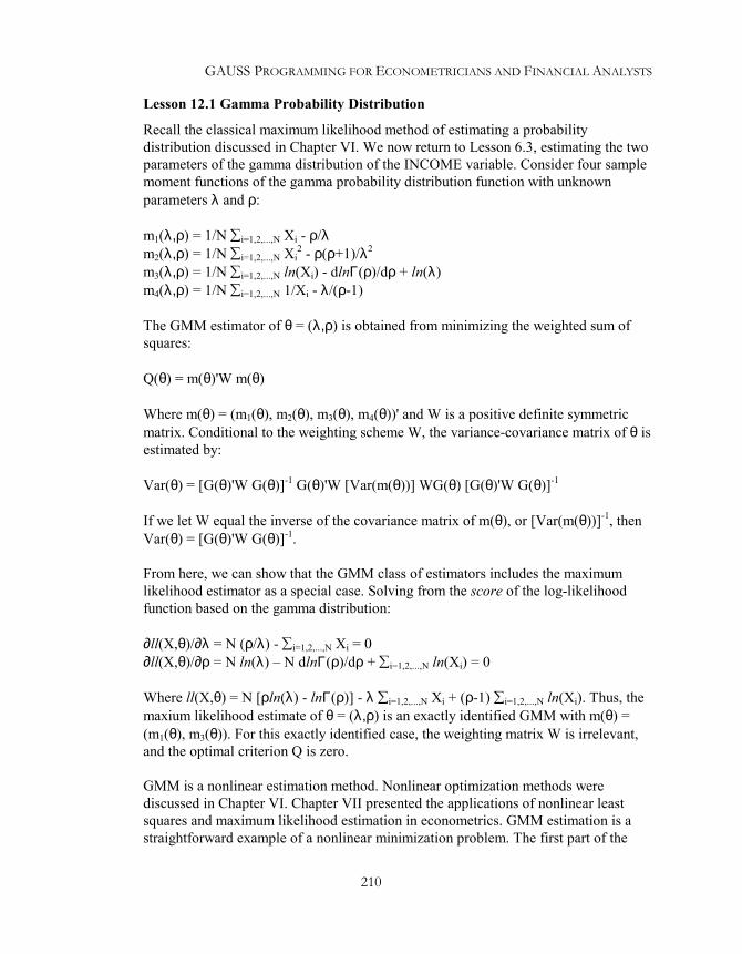
GAUSS PROGRAMMING FOR ECONOMETRICIANS AND FINANCIAL ANALYSTS
210
Lesson 12.1 Gamma Probability Distribution
Recall the classical maximum likelihood method of estimating a probabilitydistribution discussed in Chapter VI. We now return to Lesson 6.3, estimating the twoparameters of the gamma distribution of the INCOME variable. Consider four samplemoment functions of the gamma probability distribution function with unknownparameters λ and ρ:
m1(λ,ρ) = 1/N ∑i=1,2,...,N Xi - ρ/λm2(λ,ρ) = 1/N ∑i=1,2,...,N Xi
2 - ρ(ρ+1)/λ2
m3(λ,ρ) = 1/N ∑i=1,2,...,N ln(Xi) - dlnΓ(ρ)/dρ + ln(λ)m4(λ,ρ) = 1/N ∑i=1,2,...,N 1/Xi - λ/(ρ-1)
The GMM estimator of θ = (λ,ρ) is obtained from minimizing the weighted sum ofsquares:
Q(θ) = m(θ)'W m(θ)
Where m(θ) = (m1(θ), m2(θ), m3(θ), m4(θ))' and W is a positive definite symmetricmatrix. Conditional to the weighting scheme W, the variance-covariance matrix of θ isestimated by:
Var(θ) = [G(θ)'W G(θ)]-1 G(θ)'W [Var(m(θ))] WG(θ) [G(θ)'W G(θ)]-1
If we let W equal the inverse of the covariance matrix of m(θ), or [Var(m(θ))]-1, thenVar(θ) = [G(θ)'W G(θ)]-1.
From here, we can show that the GMM class of estimators includes the maximumlikelihood estimator as a special case. Solving from the score of the log-likelihoodfunction based on the gamma distribution:
∂ll(X,θ)/∂λ = N (ρ/λ) - ∑i=1,2,...,N Xi = 0∂ll(X,θ)/∂ρ = N ln(λ) – N dlnΓ(ρ)/dρ + ∑i=1,2,...,N ln(Xi) = 0
Where ll(X,θ) = N [ρln(λ) - lnΓ(ρ)] - λ ∑i=1,2,...,N Xi + (ρ-1) ∑i=1,2,...,N ln(Xi). Thus, themaxium likelihood estimate of θ = (λ,ρ) is an exactly identified GMM with m(θ) =(m1(θ), m3(θ)). For this exactly identified case, the weighting matrix W is irrelevant,and the optimal criterion Q is zero.
GMM is a nonlinear estimation method. Nonlinear optimization methods werediscussed in Chapter VI. Chapter VII presented the applications of nonlinear leastsquares and maximum likelihood estimation in econometrics. GMM estimation is astraightforward example of a nonlinear minimization problem. The first part of the

GENERALIZED METHOD OF MOMENTS
211
program Lesson 12.1 sets up a standard nonlinear optimization problem. The dataseries INCOME is read from the text file yed20.txt. As in Lesson 6.3, the INCOMEvariable is scaled by 10 and renamed x (line 4)12. The next few lines specify theminimization problem (_nlopt=0 in line 6) to be estimated by the QHC method(_method=5 in line7) with no more than 100 iterations (_iter=100 in line 8).Line 9 specifies the initial values of the two parameters ρ and λ, respectively.
1234
5678
910
11
12131415
16
17181920212223242526
/*** Lesson 12.1: GMM Estimation of a Gamma Distribution** See Greene (1999), Example 4.26 and Example 11.4*/use gpe2;output file=gpe\output12.1 reset;load data[21,2]=gpe\yed20.txt;x=data[2:21,1]/10; @ income: data scaling may help @
call reset;_nlopt=0; @ it is a minimization problem @_method=5;_iter=100;
_b=3,1; @ initial values of parameters @_hacv=1; @ hetero consistent covariance @
@ assuming serially uncorrelated @call estimate(&gmmqw,x);
@ using the results of previous estimator @_b=__b; @ for initial value of parameters and @gmmw=invpd(gmmv(x,_b)); @ for computing the weight matrix @call estimate(&gmmqw,x);call gmmout(x,__b); @ print GMM output @/*_b=__b;call estimate(&gmmq,x);call gmmout(x,__b); @ print GMM output @*/end;
/*User-defined moments equations, must be named mfbased on gamma distribution: b[1]=rho, b[2]=lambda*/proc mf(x,b);
local n,m;n=rows(x);m=zeros(n,4);m[.,1]=x-b[1]/b[2];m[.,2]=x^2-b[1]*(b[1]+1)/(b[2]^2);m[.,3]=ln(x)-gradp(&lngamma,b[1])+ln(b[2]);m[.,4]=1/x-b[2]/(b[1]-1);retp(m);
endp;
12 Our implementation of this example is slightly different from that of Example 11.4 in Greene(1999). Instead of using the scaled moment equations as Greene did, we scale the data seriesfirst and then estimate the original moment equations as described. The numerical results aremore stable and easier for evaluation.

GAUSS PROGRAMMING FOR ECONOMETRICIANS AND FINANCIAL ANALYSTS
212
27
28
/*Log of gamma distribution function*/fn lngamma(x)=ln(gamma(x));
#include gpe\gmm.gpe;
Most of the computation details and algorithms of GMM estimation in GAUSS aregrouped in a module named GMM.GPE. There are many ways to include a module inyour program. The simplest is to use the GAUSS compiler directive #include. Itwill include the specified module during the compilation of your program. We suggestincluding the module GMM.GPE at the end of your program. If you have properlyinstalled the GPE package with your version of GAUSS, GMM.GPE is located in theGPE sub-directory. Putting source codes in a separate file hides the secret ofimplementation. If you are interested in the programming details, you can examine theprogram listing of GMM.GPE also available in Appendix B-1.
The module GMM.GPE defines two objective functions, gmmqw and gmmq. Theformer uses a predefined weighting matrix, while the latter computes the weightingmatrix together with the unknown parameters. In addition, the procedure gmmoutprints the regression output. Since GMM is a nonlinear optimization method, itrequires a user-defined moment function with the name mf which, like the otherfunctions (e.g. residual function for nonlinear least squares or maximum likelihoodestimation), depends on a sample data matrix x and a parameter vector b.
Based on the gamma probability distribution, two parameters λ and ρ will beestimated from the four moment functions we defined earlier (see lines 17 through 26which define the procedure mf(x,b)). One tricky part is computing the derivative ofthe log of the gamma function for the third moment equation (line 23). The logarithmof the gamma function is defined as a separate one-line function in line 27, so that theGAUSS built-in gradient function gradp is applied in line 23.
One of the key advantages of GMM is that it allows for a flexible specification ofcovariance structure, including heteroscedasticity and autocorrelation. We have seenthe use of the GPE control variable _hacv, in Chapter IX on heteroscedasticity, andin Chapter X on autocorrelation, to compute the heteroscedasticity-autocorrelation-consistent covariance matrix. _hacv is used similarly for nonlinear GMM estimation,except that heteroscedasticity-consistent covariance is the default option here. If weassume first-order autocovariance, then line 10 needs to be modified as follows:
_hacv = 1,1;
The first element of _havc directs the computation of the heteroscedasticity-consistent covariance matrix, while the second element specifies the order of

GENERALIZED METHOD OF MOMENTS
213
autocovariance requested. See Appendix A for more information about the globalcontrol variable _hacv.
We begin the GMM estimation by minimizing the objective function gmmqw (line 11)with the default weighting matrix I (identity matrix). The estimated parameters areused as starting point for the next iteration. First, we start from the estimatedparameters (line 12) and compute the corresponding weighting matrix (line 13). Thenthe improved consistent parameter estimates are obtained (line 14) and printed (line15). We could continue on updating the weighting matrix and estimating theparameters until convergence. Equivalently, we could estimate the parameters togetherwith the associated weighting matrix. However, finding a convergent solution is notguaranteed due to high degree of non-linearity in the objective function.
Running Lesson 12.1, the first set of GMM estimation result, based on the identityweighting matrix, is as follows:
Non-Linear Optimization: Minimization Problem---------------------------------------------Assuming Generalized Method of MomentsNumber of Observations = 20Number of Parameters = 2
Maximum Number of Iterations = 100Step Size Search Method = 0Convergence Criterion = 0Tolerance = 0.001
Initial Result:Function Value = 6.4658Parameters = 3.0000 1.0000
Using Quadratic Hill-Climbing AlgorithmIteration = 1 Step Size = 1.0000 Value = 1.9867Parameters = 3.0010 0.86896…Iteration = 8 Step Size = 1.0000 Value = 0.0068077Parameters = 2.3691 0.74112
Final Result:Iterations = 8 Evaluations = 123Function Value = 0.0068077Parameters = 2.3691 0.74112Gradient Vector = -0.21423 0.44266
Asymptotic AsymptoticParameter Std. Error t-Ratio
X1 2.3691 0.010345 229.02X2 0.74112 0.0028050 264.21
The second set of GMM estimation result is based on the previous estimates of theparameters and the associated weighting matrix (see lines 12-14 of the program

GAUSS PROGRAMMING FOR ECONOMETRICIANS AND FINANCIAL ANALYSTS
214
Lesson 12.1). As is standard practice in nonlinear optimization, the estimated standarderrors and t-ratios of the parameters are computed from the inverse of the hessianmatrix calculated during minimization of the quadratic criterion function. Note thatthese are not the GMM estimates of the standard errors and t-ratios. The correctestimates of the standard errors and t-statistics of the parameters are computed at theend. In addition, the Hansen test statistic of the moment restrictions is presented.Calling the procedure gmmout (see line 15 of the program Lesson 12.1) gives us thefollowing result:
Non-Linear Optimization: Minimization Problem---------------------------------------------Assuming Generalized Method of MomentsNumber of Observations = 20Number of Parameters = 2
Maximum Number of Iterations = 100Step Size Search Method = 0Convergence Criterion = 0Tolerance = 0.001
Initial Result:Function Value = 13.294Parameters = 2.3691 0.74112
Using Quadratic Hill-Climbing AlgorithmIteration = 1 Step Size = 1.0000 Value = 9.3992Parameters = 3.3687 0.74667…Iteration = 5 Step Size = 0.5000 Value = 3.2339Parameters = 2.8971 0.84839
Final Result:Iterations = 5 Evaluations = 103Function Value = 3.2339Parameters = 2.8971 0.84839Gradient Vector = -487.16 -6.2162
Asymptotic AsymptoticParameter Std. Error t-Ratio
X1 2.8971 0.0079292 365.37X2 0.84839 0.062556 13.562
GMM Estimation Result=====================
Parameter Std. Error t-Ratio2.8971 0.0044004 658.370.84839 0.11996 7.0721
Hansen Test Statistic of the Moment RestrictionsChi-Sq( 2) = 4.4604

GENERALIZED METHOD OF MOMENTS
215
For the two parameters of the gamma distribution, ρ and λ, we now compare theirGMM estimators with the maximum likelihood (ML) estimators obtained earlier fromLesson 6.3 in Chapter VI. The standard errors are in parentheses.
ML GMMρ 2.4106 (0.7161) 2.8971 (0.0044)λ 0.7707 (0.2544) 0.8484 (0.120)
GMM Estimation of Econometric ModelsThe GMM estimation of econometric models can be considered as an extension of theinstrumental variable (IV) estimation method. IV estimation is widely used for modelswith random regressors (e.g. lagged dependent variable) which exhibitcontemporaneous correlation with the model’s errors. The advantage of GMM overIV is that the model need not be homoscedastic and serially independent. Thecovariance matrix of the averages of sample moments is taken into account forminimizing the GMM criterion function.
For notational convenience, let X be a combined data matrix of endogenous(dependent) and predetermined (independent or explanatory) variables in the model. βis a K-element vector of unknown parameters. Suppose there are L moment equations,m(X,β) = (m1(X,β), ..., mL(X,β)), where L ≥ K. The model formulation is not limitedto the case of single equation. Generalization to a system of linear or nonlinearequations is straightforward.
Corresponding to the moment conditions E(m(X,β)) = 0, we write the sample momentequations as follows:
m(β) = 1/N ∑i=1,2,...,N m(Xi,β)' = 0
Recall that the objective function, known as the GMM criterion function, to beminimized is Q(β) = m(β)'W m(β). We would optimally choose W to be equal to[Var(m(β))]-1. To find the β* which minimizes Q(β), we solve the zero-gradientconditions: ∂Q(β*)/∂β = 0. Our estimator β* of β will be asymptotically efficient andnormally distributed with mean β and covariance matrix:
Var(β*) = G(β*)'[Var(m(β*))]-1G(β*)-1
Where G(β*) = ∂m(β*)/∂β and [Var(m(β*))] is the White-Newey-West estimator ofthe covariance matrix of the sample moments.

GAUSS PROGRAMMING FOR ECONOMETRICIANS AND FINANCIAL ANALYSTS
216
Nonlinear IV Estimation
Now we consider the regression model ε = ε(β) = F(Y,X,β) (or Y- f(X,β)), where Y isthe endogenous or dependent variable, and X consists of predetermined (orindependent) variables. β is a K-element parameter vector. Let Z be a set of Linstrumental variables, for which we assume L ≥ K. Under the general assumption thatE(ε) = 0 and Var(ε) = E(εε') = Σ = σ2Ω, we can write the model as E(Z'ε) = 0. Thesample moment functions are defined by m(β) = 1/N Z'ε(β) with covariance matrix:
Var(m(β)) = 1/N2 Z' E[ε(β)ε(β)'] Z = 1/N2 Z'Σ(β)Z
Therefore, GMM estimation amounts to finding the β* which minimizes:
Q(β) = ε(β)'Z [Z'Σ(β)Z]-1Z'ε(β)
The resulting GMM estimator β* is asymptotically normally distributed with mean βand covariance matrix:
Var(β*) = (∂ε(β*)/∂β)'Z [Z'Σ(β*)Z]-1Z'(∂ε(β*)/∂β)-1
Where Σ(β∗ ) is the White-Newey-West estimator of Σ = σ2Ω.
Linear IV Estimation
If the model is linear, or ε = ε(β) = Y - Xβ, then the GMM estimator of β isequivalent to the IV estimator:
β* = (X'Z[Z'Σ(β∗ )Z]-1Z'X)-1 X'Z[Z'Σ(β∗ )Z]-1Z'YVar(β*) = X'Z[Z'Σ(β∗ )Z]-1Z'X -1
If the instrumental variables Z = X, then
β* = (X'X)-1X'YVar(β*) = (X'X)-1[X'Σ(β∗ )X](X'X)-1
Special Cases
If the IV model is homoscedastic and serially uncorrelated, that is Σ = σ2I, then
β* = (X'Z[Z'Z]-1Z'X)-1X'Z[Z'Z]-1Z'YVar(β*) = σ2(β∗ ) X'Z[Z'Z]-1Z'X-1
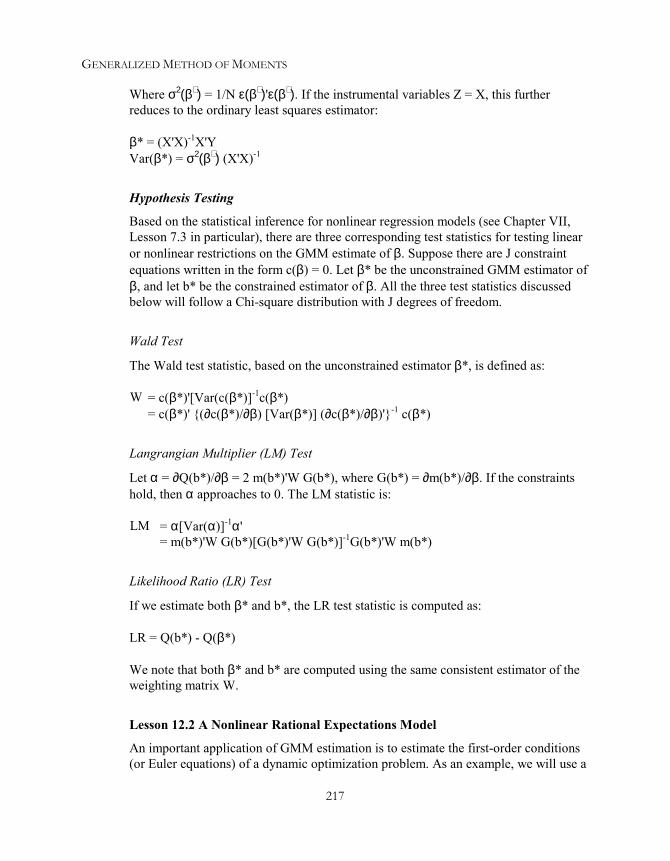
GENERALIZED METHOD OF MOMENTS
217
Where σ2(β∗ ) = 1/N ε(β∗ )'ε(β∗ ). If the instrumental variables Z = X, this furtherreduces to the ordinary least squares estimator:
β* = (X'X)-1X'YVar(β*) = σ2(β∗ ) (X'X)-1
Hypothesis Testing
Based on the statistical inference for nonlinear regression models (see Chapter VII,Lesson 7.3 in particular), there are three corresponding test statistics for testing linearor nonlinear restrictions on the GMM estimate of β. Suppose there are J constraintequations written in the form c(β) = 0. Let β* be the unconstrained GMM estimator ofβ, and let b* be the constrained estimator of β. All the three test statistics discussedbelow will follow a Chi-square distribution with J degrees of freedom.
Wald Test
The Wald test statistic, based on the unconstrained estimator β*, is defined as:
W = c(β*)'[Var(c(β*)]-1c(β*)= c(β*)' (∂c(β*)/∂β) [Var(β*)] (∂c(β*)/∂β)'-1 c(β*)
Langrangian Multiplier (LM) Test
Let α = ∂Q(b*)/∂β = 2 m(b*)'W G(b*), where G(b*) = ∂m(b*)/∂β. If the constraintshold, then α approaches to 0. The LM statistic is:
LM = α[Var(α)]-1α'= m(b*)'W G(b*)[G(b*)'W G(b*)]-1G(b*)'W m(b*)
Likelihood Ratio (LR) Test
If we estimate both β* and b*, the LR test statistic is computed as:
LR = Q(b*) - Q(β*)
We note that both β* and b* are computed using the same consistent estimator of theweighting matrix W.
Lesson 12.2 A Nonlinear Rational Expectations Model
An important application of GMM estimation is to estimate the first-order conditions(or Euler equations) of a dynamic optimization problem. As an example, we will use a

GAUSS PROGRAMMING FOR ECONOMETRICIANS AND FINANCIAL ANALYSTS
218
model common in the finance literature. Suppose a representative stockholder atcurrent time t, who tries to maximize a concave expected utility function ofconsumption over an indefinite future horizon:
∑τ=0,...,∞ βτ Eu(Ct+τ) | Zt
Where Zt is the information available to the consumer at time t and Ct+τ is theconsumption τ periods from t. 0 < β <1 is known as the discount factor of timepreference. Given N different stocks, the optimal consumption-investment allocationmust satisfy the following condition:
u'(Ct) = β Eu'(Ct+1) [(Pi,t+1+Di,t+1)/Pt] | Zt
for i = 1,...,N. u'(Ct) = ∂u/∂Ct is the marginal utility of consumption at time t. Pi,t+1 isthe price of stock i at time t+1 and Di,t+1 is the dividend per share of stock i at t+1. Theratio (Pi,t+1+Di,t+1)/Pi,t represents the returns of investment in stock i between periods tand t+1. In other words, this merely defines the equilibrium condition that themarginal utility of consumption in the current period must equal the expected returnnext period from investing in stock i. Assume that the utility function exhibits constantrelative risk aversion as:
u(Ct) = Ctα/α for α<1.
where 1-α is known as the coefficient of relative risk aversion, and 1-α > 0. Then, foreach i = 1, ..., N, the optimal decision-rule is
Ctα-1 = β ECt+1
α-1 [(Pi,t+1+Di,t+1)/Pt] | Zt
Equivalently, for each stock i = 1, ..., N, we must have
βE[(Ct+1/Ct)α-1] [(Pi,t+1+Di,t+1)/Pt] | Zt = 1
The hypothesis of rational expectations assumes that the intertemporal decision-making should be independent from the historical information available at the time atwhich the decision is made. Therefore, the derived orthgonality condition for eachstock i = 1, ..., N is:
E [Zt β[(Ct+1/Ct)α-1] [(Pi,t+1+Di,t+1)/Pt] -1] = 0

GENERALIZED METHOD OF MOMENTS
219
For more detailed description of the model, see Hansen and Singleton (1982)13. Interms of our econometric estimation, the model may be expressed with theorthogonality condition: E[Z ε(X,θ)] = 0, where X = [X1,X2,X3], θ = (β,α), and
ε(X,θ) = [βX1α−1X2 – 1, βX1
α−1X3 – 1]
The data file gmmq.txt installed in the GPE sub-directory consists of three variables(335 observations from January 1959 to December 1978, though not the originalHansen-Singleton data):
X1 Ratio of two-period consumption, Ct+1/Ct.X2 Value-weighted returns of NYSE stock market, (Pt+1+Dt+1)/Pt where Pt+1 is the
price and Dt+1 is the dividend payoff of stock at t+1.X3 Risk-free rate of returns (T-Bill rate).
We note that this model consists of a system of two nonlinear equations. Theinstrumental variables Z consist of one or several lags of X and a constant. Thefollowing program Lesson 12.2 implements and estimates the Hansen-Singletonrational expectations model. The program structure looks similar to that of Lesson12.1. The main difference is the model specification described in the block from line19 to line 27 for the moment function procedure mf(x,b), which reflects exactly themodel described above. We use one lag of each of the three variables X1, X2, X3, anda constant as the instrumental variables (see line 22). More lags may be included forthe additional instrumental variables. The two orthgonality equations for stock andrisk-free returns are concatenated to form the moment functions system (see lines 23and 24). The rest of the program performs the GMM estimation. First, the initialestimates of (β,α) are obtained by assuming the default identity weighting matrix inthe objective function for minimization (line 10). Then, with the resulting covariancematrix of the moment functions, the consistent parameter estimates are calculated (seelines 11-13). An efficient solution is obtained from simultaneously estimating theparameters and the corresponding covariance matrix in the second iteration (see lines15 and 16).
123
/*** Lesson 12.2: A Nonlinear Rational Expectation Model** GMM Estimation of Hansen-Singleton Model (Ea, 1982)*/use gpe2;output file=gpe\output12.2 reset;load x[335,3]=gpe\gmmq.txt; @ data columns: @
@ (1) c(t+1)/c(t) (2)vwr (3)rfr @
13 For computational implementation of the model and the data file gmmq.txt used in thislesson example, see also the Hasen-Heaton-Ogaki GMM package from the AmericanUniversity GAUSS archive at http://www.american.edu/academic.depts/cas/econ/gaussres/GMM/GMM.HTM.

GAUSS PROGRAMMING FOR ECONOMETRICIANS AND FINANCIAL ANALYSTS
220
45678
910
111213
14
1516
17
18
192021222324252627
28
call reset;_nlopt=0;_method=5;_tol=1.0e-5;_iter=100;
_b=1,0; @ GMM estimation with initial @call estimate(&gmmqw,x); @ identity weighting matrix @
_b=__b; @ GMM estimation with external @gmmw=invpd(gmmv(x,__b)); @ covariance weighting matrix @call estimate(&gmmqw,x);
call gmmout(x,__b); @ print GMM output @
_b=__b; @ there may be a convergent efficient soultion@call estimate(&gmmq,x); @ with internal covariance weighting matrix @
call gmmout(x,__b); @ print GMM output @
end;
/*User-defined moments functions, must be named mf*/proc mf(x,b);
local z,n,m;n=rows(x);z=ones(n,1)~lagn(x,1); @ IV @m=z.*(b[1]*(x[.,1]^(b[2]-1)).*x[.,2]-1);m=m~(z.*(b[1]*(x[.,1]^(b[2]-1)).*x[.,3]-1));@ nonlinear multiple equations system @retp(packr(m));
endp;
#include gpe\gmm.gpe;
The first part of the output (the first iteration, using the identity matrix as theweighting matrix) is only preparation for computing the consistent parameterestimates in the second iteration of the GMM estimation. The result of secondconsistent estimation is shown below:
Non-Linear Optimization: Minimization Problem---------------------------------------------Assuming Generalized Method of MomentsNumber of Observations = 335Number of Parameters = 2
Maximum Number of Iterations = 100Step Size Search Method = 0Convergence Criterion = 0Tolerance = 1e-005
Initial Result:Function Value = 55.406Parameters = 0.99977 -0.00012883

GENERALIZED METHOD OF MOMENTS
221
Using Quadratic Hill-Climbing AlgorithmIteration = 1 Step Size = 1.0000 Value = 19.924Parameters = 1.0014 0.00045142…Iteration = 13 Step Size = 1.4641 Value = 9.4685Parameters = 0.99919 0.85517
Final Result:Iterations = 13 Evaluations = 239Function Value = 9.4685Parameters = 0.99919 0.85517Gradient Vector = -0.00026951 0.00017303
Asymptotic AsymptoticParameter Std. Error t-Ratio
X1 0.99919 0.00012573 7946.9X2 0.85517 0.044497 19.219
GMM Estimation Result=====================
Parameter Std. Error t-Ratio0.99919 0.00047887 2086.60.85517 0.17853 4.7901
Hansen Test Statistic of the Moment RestrictionsChi-Sq( 6) = 13.306
The consistent estimates (0.9992, 0.8552) of the two parameters are obtained using 8instrument variables (4 for each of the two equations). The Hansen test statistic of theextra 6 moment restrictions is barely statistically significant at 5 percent level (withthe critical value 12.59).
Non-Linear Optimization: Minimization Problem---------------------------------------------Assuming Generalized Method of MomentsNumber of Observations = 335Number of Parameters = 2
Maximum Number of Iterations = 100Step Size Search Method = 0Convergence Criterion = 0Tolerance = 1e-005
Initial Result:Function Value = 13.306Parameters = 0.99919 0.85517
Using Quadratic Hill-Climbing AlgorithmIteration = 1 Step Size = 1.0000 Value = 12.590Parameters = 0.99934 0.85482…Iteration = 7 Step Size = 0.0039 Value = 12.474Parameters = 0.99950 0.78735
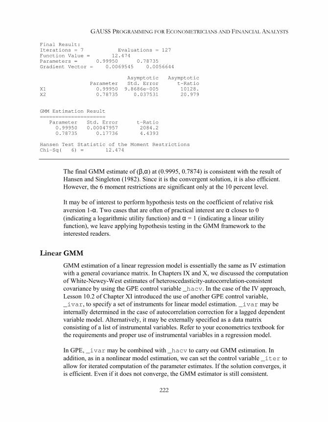
GAUSS PROGRAMMING FOR ECONOMETRICIANS AND FINANCIAL ANALYSTS
222
Final Result:Iterations = 7 Evaluations = 127Function Value = 12.474Parameters = 0.99950 0.78735Gradient Vector = 0.0069545 0.0056644
Asymptotic AsymptoticParameter Std. Error t-Ratio
X1 0.99950 9.8686e-005 10128.X2 0.78735 0.037531 20.979
GMM Estimation Result=====================
Parameter Std. Error t-Ratio0.99950 0.00047957 2084.20.78735 0.17736 4.4393
Hansen Test Statistic of the Moment RestrictionsChi-Sq( 6) = 12.474
The final GMM estimate of (β,α) at (0.9995, 0.7874) is consistent with the result ofHansen and Singleton (1982). Since it is the convergent solution, it is also efficient.However, the 6 moment restrictions are significant only at the 10 percent level.
It may be of interest to perform hypothesis tests on the coefficient of relative riskaversion 1-α. Two cases that are often of practical interest are α closes to 0(indicating a logarithmic utility function) and α = 1 (indicating a linear utilityfunction), we leave applying hypothesis testing in the GMM framework to theinterested readers.
Linear GMMGMM estimation of a linear regression model is essentially the same as IV estimationwith a general covariance matrix. In Chapters IX and X, we discussed the computationof White-Newey-West estimates of heteroscedasticity-autocorrelation-consistentcovariance by using the GPE control variable _hacv. In the case of the IV approach,Lesson 10.2 of Chapter XI introduced the use of another GPE control variable,_ivar, to specify a set of instruments for linear model estimation. _ivar may beinternally determined in the case of autocorrelation correction for a lagged dependentvariable model. Alternatively, it may be externally specified as a data matrixconsisting of a list of instrumental variables. Refer to your econometrics textbook forthe requirements and proper use of instrumental variables in a regression model.
In GPE, _ivar may be combined with _hacv to carry out GMM estimation. Inaddition, as in a nonlinear model estimation, we can set the control variable _iter toallow for iterated computation of the parameter estimates. If the solution converges, itis efficient. Even if it does not converge, the GMM estimator is still consistent.

GENERALIZED METHOD OF MOMENTS
223
Lesson 12.3 GMM Estimation of U. S. Consumption Function
In the following, we present a simple example of a consumption function derived fromHall’s Life Cycle-Permanent Income Hypothesis (Hall, 1978) with a quadratic utilityfunction. The intertemporal model formulation is similar to that of Lesson 12.2 on theconsumption-investment decision-making, with the exception that we consider onlythe consumption plan with a quadratic utility function. The use of a quadraticfunctional form leads to a linear consumption function:
Ct+1 = β0 + β1Ct + εt+1
Ct+1 and Ct are expected and current consumption, respectively. Let Zt be historicalinformation available to the consumer at time t or earlier. Then the orthogonalitycondition becomes:
E(Ztεt+1) = 0
From other theories of consumption, the instrumental variables Z may include level ofincome Y and consumption C in addition to a constant. That is,
Zt = [ 1 Ct Yt]
Further lags of C and Y may be added to the model as needed. The consumption-income relationship was studied in Chapter XI with income as the explanatoryvariable. Based on an Euler equation of a constrained expected utility maximization,in this example, the future consumption is affected indirectly by the current and pastincome as the instrumental variables. Using the U. S. time series data of usyc87.txt,Lesson 12.3 demonstrates GMM estimation of the linear consumption function asfollows:
12
345
67891011
/*** Lesson 12.3: GMM Estimation of U. S. Consumption Function** GMM Estimation of a Linear Regression Model*/use gpe2;output file=gpe\output12.3 reset;
load z[67,3]=gpe\usyc87.txt;y = z[2:67,2];c = z[2:67,3];
call reset;_names="c","c1";_rstat=1;_rplot=2;_dlags=1;_ivar=ones(rows(y),1)~lagn(c~y,1);

GAUSS PROGRAMMING FOR ECONOMETRICIANS AND FINANCIAL ANALYSTS
224
1213
14
15
_hacv=1,1;_iter=100;
call estimate(c,0);
end;
Two variables named C and Y, are read from the data file usyc87.txt. Line 10,_dlags = 1, specifies the lagged dependent variable model. GMM estimation forthe linear autoregressive consumption function is given in line 14, with theinstrumental variables _ivar specified in line 11. We use only the first lag of incomeand consumption variables in addition to a constant as the instruments. The first-orderautocovariance structure is specified in line 12, in which the White-Newey-Westestimate will be computed. The computation of GMM estimates will be iterated untilconvergence or until the limit set in line 13, _iter = 100. The empirical results ingreat detail can be found in the output file output12.3.
Of course the estimated model is not good enough to be free of misspecification. Itserves the purpose for demonstrating GMM estimation of a linear model. To improvethe model, either more lags of consumption should be included for a comprehensiveautoregressive specification or the model should explicitly correct for serialcorrelation. We leave the rest of the model improvement task to the interested reader.

XIIISystem of Simultaneous Equations
GPE can estimate systems of linear and nonlinear equations. For a system of linearequations, you need to define the endogenous and predetermined (including laggedendogenous, current and lagged exogenous) variables. By selecting and identifying therelevant variables for each equation, the procedure estimate carries out the systemmodel estimation as in the case of a single equation model. For a system of nonlinearequations, it becomes more involved to define the functional form for the modelequations. In this chapter, the classic example of Klein Model I (1950) is used todemonstrate the estimation of a system of linear regression equations. The special caseof Seemingly Related Regressions (SUR) is considered with the Berdnt-Wood Modelof energy demand. Finally, re-examining the Klein Model, nonlinear maximumlikelihood estimation is shown to be useful for estimating a system of nonlinearequations.
Linear Regression Equations SystemWe follow the conventional matrix representation of a system of linear equations as:
YB + XΓ = U
Let N be the number of observations, G be the number of endogenous variables(therefore, the number of equations), and K be the number of predetermined variables.Then Y, a N×G matrix, and X, a N×K matrix, are the respective data matrices ofendogenous and predetermined variables. The corresponding G×G matrix Bassociated with the endogenous variable matrix Y and the G×K matrix Γ associatedwith predetermined variable matrix X are the sparse parameter matrices in which theunknown nonzero elements need to be estimated. Finally, U is the N×G stochasticerror matrix.
Given the data matrices Y and X, the unknown parameters in B and Γ can beestimated using a variety of methods. GPE implements both single equation (limitedinformation) methods and simultaneous equations (full information) methods. Beforethe parameter estimation, the model of multiple equations must be properly specifiedto account for the relevant variables and restrictions. In GPE, this is done byspecifying the structure of the parameter matrices B and Γ. It uses a couple ofspecification matrices to define the stochastic equations and fixed identities of the

GAUSS PROGRAMMING FOR ECONOMETRICIANS AND FINANCIAL ANALYSTS
226
system by representing the parameter matrices of the system as arrays of 1’s, 0’s, and–1’s, signifying the inclusion or exclusion of variables from particular equations. Inthe following, we discuss the three most important input variables that control thespecification and estimation of a simultaneous linear equations model.
• _eq• _id• _method
First, the variable _eq specifies the stochastic equation matrix for system modelestimation. This is a Gs by (G+K) matrix with elements -1, 0, and 1 arranged inaccordance with the order of endogenous variables Y followed by the predeterminedvariables X. Note that Gs is the number of stochastic equations and G ≥ Gs. For eachstochastic equation, there is exactly one row of _eq to define it. In the stochasticequation specification matrix _eq, an element -1 indicates the left-hand-sideendogenous variable. Only one -1 entry is allowed in each equation. An element 1indicates the use of an endogenous and/or a predetermined variable on the right-hand-side of an equation. The zeros indicate the corresponding unused or excludedvariables in the equation. Constant terms are not normally included in the equationspecification. If _eq is not specified, or _eq=0 by default, a seemingly unrelatedregression equations system is assumed. In this case, Gs = G, and the _eq matrixconsists of a G×G sub-matrix with -1 in the diagonals and zeroes elsewhere(endogenous variables portion of _eq), and a G×K sub-matrix consisting entirety ofones (predetermined variables portion of _eq).
The second input variable _id specifies the identity equation specification matrix fora system model. _id is similar in size and setup to _eq, except that its entries can beany value as required by the model. If _id is not specified, or _id=0 by default,there is no identity. To ensure the system compatibility, the number of rows in twospecification matrices _eq and _id must sum to G, the total number of endogenousvariables or equations in the system.
The input variable _method controls the use of specific method of estimation. In thecontext of simultaneous linear equations, the available estimation methods are:
_method=0 Ordinary Least Squares (OLS, the default method)_method=1 Limited Information Maximum Likelihood (LIML)_method=2 Two-Stage Least Squares (2SLS)_method=3 There-Stage Least Squares (3SLS, may be iterative)_method=4 Full Information Maximum Likelihood (FIML, may be
iterative)

SYSTEM OF SIMULTANEOUS EQUATIONS
227
Note that LIML and FIML are not true nonlinear maximum likelihood estimationmethods. Instead they are types of instrumental variables estimation. In GPE, threevariants of the FIML method are available:
_method=4,0 (or 4) FIML Instrumental variable method (Hausman, 1975)_method=4,1 FIML Linearized method (Dhrymes, 1970)_method=4,2 FIML Newton method
2SLS and 3SLS are flavors of the instrumental variables estimation method, where theinstrumental variables used are all the predetermined variables in the system. Forestimation of a linear system model, external instrumental variables may be requestedand specified in the matrix _ivar. The data matrix _ivar will be combined with allthe predetermined variables to form the basis for instrumental variable estimation. Aconstant term is automatically included in _ivar. For technical details andcomparisons of different estimation methods for a linear equations system, refer toyour econometrics textbook.
Klein Model I (1950)
The pedagogical example of Klein Model I is typically used to demonstrate the modelestimation of a linear regression equations system. It was the first U. S. economy-wideeconometric model consisting of three stochastic equations with about 10 variablescovering the prewar period from 1920 to 1941. klein.txt is a text data file containingthese variables used in the Klein Model I. There are several variations of the KleinModel in the literature. For the convenience of illustration, we adopt the followingspecification of the model:
C = α0 + α1 P + α2 P-1 + α3 (W1 + W2) + ε1
I = β0 + β1 P + β2 P-1 + β3 K + ε2
W1 = γ0 + γ1 X + γ2 X-1 + γ3 A + ε3X = C + I + GP = X – T – W1K = K-1 + I
Where the variables used are:
C Consumption in billions of 1934 dollars.I Investment.W1 Private wage bill.X Total private income before taxes, or X = Y + T - W2 where Y is after-tax
income.P Private profits.K Capital stock in the beginning of year, or capital stock lagged one year.

GAUSS PROGRAMMING FOR ECONOMETRICIANS AND FINANCIAL ANALYSTS
228
W2 Government wage bill.G Government non-wage spending.T Indirect taxes plus net exports.A Year – 1931 (a time trend).
The first three equations are stochastic with unknown parameters α’s, β’s, and γ’s,respectively. The rest of three equations are accounting identities. Since the sum ofprivate and public wage bills (W1+W2) appears in the first equation, it is moreconvenient to introduce one additional endogenous variable W, total wage bill, withthe accounting identity:
W = W1 + W2
The alternative is to impose a linear parameter restriction of identical parameter valuefor W1 and W2 in the first equation. The resulting model consists of 7 endogenousvariables (C, I, W1, X, P, K, W) and 8 predetermined variables (X-1, P-1, K-1, W2, G,T, A, and Constant). Lesson 13.1 below implements the model as described.
Lesson 13.1: Klein Model I
In the program, from line 3 to line 15, the data file klein.txt is loaded and eachvariable used in the model is defined. Data matrix yvar of endogenous variables isdefined in Line 16. Line 17 defines the data matrix xvar of predetermined variableswhich includes three lagged endogenous variables and four exogenous variables. Bydefault, a constant term is automatically included in each stochastic equation. Then, inthe next two lines, are the two important control variables: _eq and _id. We explainthe construction of the first line of these two matrices, and leave you to puzzle out therest.
First, the _eq matrix (line 21) specifies which variables are to be included in whichstochastic equations. Recall the first stochastic equation in the Klein Model I:
C = α0 + α1 P + α2 P-1 + α3 (W1 + W2) + ε1
Then the first line of the _eq matrix is:
@ C I W1 X P K W XL PL KL W2 A G T 1 @_eq = -1 0 0 0 1 0 1 0 1 0 0 0 0 0, …
Note that the column under the variable C contains a –1. This means that C is the left-hand-side variable of the first stochastic equation. Since I and W1 are not in the firststochastic equation, we place 0’s in their respective columns. Looking again at thisequation, we see that the right-hand-side variables are: constant, P, P-1, W (rememberthat W = W1+ W2). To let GPE know that P, P-1, and W are in the first equation, we

SYSTEM OF SIMULTANEOUS EQUATIONS
229
place 1’s in their respective places in the _eq matrix. This does not mean that theircoefficients are restricted to be equal to one, it merely tells GPE to include thoseparticular variables in the equation. GPE includes the constant automatically. All othervariables (namely X, K, X-1, K-1, W2, A, G, T) are not in the first equation. Putting 0’sin the respective places of these variables in the _eq matrix lets GPE know that itshould not include these variables in the first stochastic equation of the system.
123
45678910111213
1415
1617
18
19
20
21
22
23
242526272829
303132
/*** Lesson 13.1: Klein's Model I** Simultaneous Equation System of Klein's Model I*/use gpe2;output file = gpe\output13.1 reset;load data[23,10] = gpe\klein.txt;
a=data[2:23,1]-1931; @ time trend: 1931 = 0 @c=data[2:23,2]; @ consumption @p=data[2:23,3]; @ profit income @w1=data[2:23,4]; @ private wage income @i=data[2:23,5]; @ investment @k1=data[2:23,6]; @ lagged capital stock @x=data[2:23,7]; @ private total income @w2=data[2:23,8]; @ public wage income @g=data[2:23,9]; @ government spending @t=data[2:23,10]; @ tax @
k=k1[2:22]|209.4; @ capital stock @w=w1+w2; @ total wage income @
yvar=c~i~w1~x~p~k~w;xvar=lag1(x~p~k)~w2~a~g~t;
call reset;
_names="c","i","w1","x","p","k","w","x-1","p-1","k-1","w2","a","g","t";
_vcov=1;@ C I W1 X P K W XL PL KL W2 A G T 1 @
_eq = -1 0 0 0 1 0 1 0 1 0 0 0 0 0,0 -1 0 0 1 0 0 0 1 1 0 0 0 0,0 0 -1 1 0 0 0 1 0 0 0 1 0 0;
_id = 1 1 0 -1 0 0 0 0 0 0 0 0 1 0,0 0 -1 1 -1 0 0 0 0 0 0 0 0 -1,0 1 0 0 0 -1 0 0 0 1 0 0 0 0,0 0 1 0 0 0 -1 0 0 0 1 0 0 0;
_begin=2;
_method=0; @ OLS estimation @call estimate(yvar,xvar);_method=1; @ LIML estimation @call estimate(yvar,xvar);_method=2; @ 2SLS estimation @call estimate(yvar,xvar);
_iter=100;_method=3; @ 3SLS estimation (iterative) @call estimate(yvar,xvar);

GAUSS PROGRAMMING FOR ECONOMETRICIANS AND FINANCIAL ANALYSTS
230
333435
_method=4; @ FIML estimation @call estimate(yvar,xvar);end;
Similarly, line 22 specifies the identity equations of the model. Take the first identityequation as an example:
X = C + I + G
It involves the variables X, C, I, and G. Therefore, in the first row of _id matrix,only the relevant columns have non-zero values. Typically these entries are 1 or –1,but they could be any other values as required. Variables not used in the definition ofan identity have zeroes in the corresponding places of _id matrix. The first row of_id matrix looks like this:
@ C I W1 X P K W XL PL KL W2 A G T 1 @_id = 1 1 0 -1 0 0 0 0 0 0 0 0 1 0, …
The easiest way to understand the construction of the system model described so faris to relate it with the matrix representation:
YB + XΓ = U
Where Y corresponds to yvar and X corresponds to xvar in the program. Thematrix _eq|_id (vertical concatenation of _eq and _id) is the specificationmatrix corresponding to the transpose of B|Γ (vertical concatenation of B and Γ).
Because the use of lag variables, the first observation of data is lost and estimationmust start from the second observation (see line 23). From line 24 through 34, fiveestimation methods are carried out. They are OLS, LIML, 2SLS, 3SLS, and FIML. Itis of interest to see the covariance matrices of the equations, thus line 20 sets theoption _vcov=1 to show variance-covariance matrix across equations and acrossparameters as well. Note that 3SLS and FIML are iterative methods, and it is wise toset an iteration limit for the solution to converge. Line 30, _iter=100, does the job.
Running the program of Lesson 13.1 will generate about 20 pages of output. To savespace, we will only present the results of 2SLS because of its popularity in theliterature. You should run the program in its entirety and check the output file to seethe complete results. In a summary table, the parameter estimates of these methods arelisted and compared. You need to check your econometrics textbook for theevaluation of the pros and cons of these estimation methods, in particular thedifferences between limited information and full information estimation methods.
The regression results of a typical linear system model are divided into two parts: theresults of the system of equations as a whole, and the results of each separate

SYSTEM OF SIMULTANEOUS EQUATIONS
231
equation. Here we present only the first part of 2SLS for the estimated parameters,including the variance-covariance matrics across equations. For the rest of regressionresults by equation, we refer to the output file output13.1.
Simultaneous Linear Equations Estimation----------------------------------------Number of Endogenous Variables = 7Number of Predetermined Variables = 8Number of Stochastic Equations = 3Number of Observations = 21Estimation Range = 2 22
Two Stages Least Squares Estimation
System R-Square = 0.97711Log-Likelihood = -121.56134
Equation Variable Estimated AsymptoticName Name Coefficient Std Error t-RatioC P 0.017302 0.11805 0.14657
W 0.81018 0.040250 20.129P-1 0.21623 0.10727 2.0158CONSTANT 16.555 1.3208 12.534
I P 0.15022 0.17323 0.86718P-1 0.61594 0.16279 3.7838K-1 -0.15779 0.036126 -4.3677CONSTANT 20.278 7.5427 2.6885
W1 X 0.43886 0.035632 12.316X-1 0.14667 0.038836 3.7767A 0.13040 0.029141 4.4746CONSTANT 1.5003 1.1478 1.3071
Asymptotic Variance-Covariance Matrix of EquationsC 1.0441I 0.43785 1.3832W1 -0.38523 0.19261 0.47643
C I W1
Asymptotic Variance-Covariance Matrix of CoefficientsP 0.013936W -0.0015260 0.0016200P-1 -0.0095710 -0.00053085 0.011506CONSTANT -0.015344 -0.032733 -0.0047520 1.7445P 0.0040375 0.0012781 -0.0046423 -0.045188 0.030008P-1 -0.0031110 -0.0011810 0.0051395 0.017372 -0.025772K-1 -0.00037500 0.00039811 -0.00013045 -0.0080439 0.0041898CONSTANT 0.057936 -0.082066 0.020400 2.1124 -0.92485X -0.0018149 5.1138E-005 0.0011799 0.0092111 0.00059433X-1 0.0018888 -8.0164E-005 -0.0017884 0.00071044 -0.00058617A 0.00066034 -0.00052372 0.00047623 0.0027719 0.00047661CONSTANT -0.00052229 0.0015772 0.032840 -0.61273 -0.0017044
P W P-1 CONSTANT P
P-1 0.026499K-1 -0.0038717 0.0013051CONSTANT 0.77760 -0.26903 56.892X -0.00033125 -9.0028E-005 0.013436 0.0012696

GAUSS PROGRAMMING FOR ECONOMETRICIANS AND FINANCIAL ANALYSTS
232
X-1 0.00061121 9.9812E-005 -0.020120 -0.0011997 0.0015082A -0.00066991 0.00017448 -0.032062 -0.00030915 5.1023E-005CONSTANT -0.015548 -0.00038089 0.36894 -0.0066842 -0.015405
P-1 K-1 CONSTANT X X-1
A 0.00084920CONSTANT 0.015608 1.3174
A CONSTANT
The system estimation methods such as 3SLS and FIML may be iterated until theconvergent solution is found. To control the iteration, as in the case of nonlineariteration methods, the following input control variables may be applied: _iter,_tol, and _restart. We refer the readers to Appendix A for more details of thesecontrol variables. For example, the statement _iter=100 of line 30 sets the numberof iterations for 3SLS and FIML estimation. This is to ensure the near efficiency(theoretically speaking) of the parameter estimates, if it is found before exhausting thelimit of iterations. It will be warned that the results may be unreliable when iterationsexceed the limit.
In Lesson 13.1, line 33:
_method = 4;
indicates that the instrumental variables method of FIML is used for estimation. It isequivalent to state the scalar 4 as a vector 4,0. The alternatives are either setting_method to 4,1 for a linearized FIML or setting it to 4,2 for the Newtonmethod. It is mind boggling that, for the same problem in hand, not all the FIMLmethods will converge to the same solution (provided there is convergence of asolution). It is now common wisdom that different methods may produce differentresults due to different algorithms in use for nonlinear model estimation.
We now present the summary table of the parameter estimates obtained from fivemethods we use in estimating the Klein Model I. Numbers in parenthesis areasymptotic standard errors.

SYSTEM OF SIMULTANEOUS EQUATIONS
233
Eq. Variable OLS LIML 2SLS 3SLS FIML/IVC P 0.19293
(0.082065)-0.22251
(0.20175)0.017302(0.11805)
0.16451(0.096198)
-0.23190(0.23178)
W 0.79622(0.035939)
0.82256(0.055378)
0.81018(0.040250)
0.76580(0.034760)
0.80182(0.037137)
P-1 0.089885(0.081559)
0.39603(0.17360)
0.21623(0.10727)
0.17656(0.090100)
0.38545(0.18362)
Const. 16.237(1.1721)
17.148(1.8403)
16.555(1.3208)
16.559(1.2244)
18.340(1.8637)
I P 0.47964(0.087377)
0.075185(0.20218)
0.15022(0.17323)
-0.35651(0.26015)
-0.80082(0.35761)
P-1 0.33304(0.090747)
0.68039(0.18817)
0.61594(0.16279)
1.0113(0.24876)
1.0516(0.30823)
K-1 -0.11179(0.024048)
-0.16826(0.040798)
-0.15779(0.036126)
-0.26019(0.050868)
-0.14811(0.033826)
Const. 10.126(4.9175)
22.591(8.5458)
20.278(7.5427)
42.895(10.593)
27.267(7.7850)
W1 X 0.43948(0.029158)
0.43394(0.067937)
0.43886(0.035632)
0.37478(0.031103)
0.23412(0.045546)
X-1 0.14609(0.033671)
0.15132(0.067054)
0.14667(0.038836)
0.19365(0.032402)
0.28464(0.042736)
A 0.13025(0.028711)
0.13159(0.032386)
0.13040(0.029141)
0.16792(0.028929)
0.23487(0.033488)
Const. 1.4970(1.1427)
1.5262(1.1884)
1.5003(1.1478)
2.6247(1.1956)
5.7963(1.7621)
Log-Likelihood -141.92156 -122.81636 -121.56134 -86.14210 -83.32381
Lesson 13.2: Klein Model I Reformulated
In Lesson 13.1, we saw the use of the input variable _begin (line 23) to control thestarting data observation for model estimation, and of _vcov (line 20) to show theestimated variance-covariance matrix of the parameters. There are many other inputvariables useful for controlling single equation model estimation are applicable to thesystem model estimation. These include, but are not limited to: _const, _dlags,_restr. In addition, for presenting the estimation results, the control variables suchas _rstat, and _rplot are useful. We refer the details of using these input controlvariables to the Appendix A: GPE Control Variables.
Lesson 13.2 below is a reformulation of Klein Model I. There are no new thingsadded. Instead, it demonstrates the use of a few input control variables mentionedabove to offer an alternative formulation of the model. This may be a more useful

GAUSS PROGRAMMING FOR ECONOMETRICIANS AND FINANCIAL ANALYSTS
234
representation for the purpose of forecasting and simulation. In the following, we willlist the program without running it.
123
45678910111213
1415
1617
18
19
20
21
22
23
24
/*** Lesson 13.2: Klein's Model I Reformulated** Using _dlags and _restr*/use gpe2;output file = gpe\output13.2 reset;load data[23,10] = gpe\klein.txt;
a=data[2:23,1]-1931; @ time trend: 1931 = 0 @c=data[2:23,2]; @ consumption @p=data[2:23,3]; @ profit income @w1=data[2:23,4]; @ private wage income @i=data[2:23,5]; @ investment @k1=data[2:23,6]; @ lagged capital stock @x=data[2:23,7]; @ private total income @w2=data[2:23,8]; @ public wage income @g=data[2:23,9]; @ government spending @t=data[2:23,10]; @ tax @
k=k1[2:22]|209.4; @ capital stock @w=w1+w2; @ total wage income @
@ do not include lagged endog. var. in xvar and _names @yvar=c~i~w1~x~p~k;xvar=w2~a~g~t;
call reset;
_names="c","i","w1","x","p","k","w2","a","g","t";
_vcov=1;
@ do not include lagged endog. var. in _eq and _id @@ C I W1 X P K W2 A G T 1 @_eq = -1 0 1 0 1 0 1 0 0 0,
0 -1 0 0 1 0 0 0 0 0,0 0 -1 1 0 0 0 1 0 0;
_id = 1 1 0 -1 0 0 0 0 1 0,0 0 -1 1 -1 0 0 0 0 -1,0 1 0 0 0 -1 0 0 0 0;
@ using _dlags option to add the specified lagged endog. var. @@ after the entire list of endog. var. in _eq and _id @@ C I W1 X P K @_dlags = 0 0 0 0 1 0,
0 0 0 0 1 1,0 0 0 1 0 0,0 0 0 0 0 0,0 0 0 0 0 0,0 0 0 0 0 1;
@ restriction: W1 and W2 share the same coef. in C eq. @@ EQ: C | I | W1 @@ VAR: W1 P P1 W2|P P1 K1|X X1 A|q **incl. lagged endog. @_restr = 1 0 0 -1 0 0 0 0 0 0 0;

SYSTEM OF SIMULTANEOUS EQUATIONS
235
2526
272829
303132
_method=2; @ 2SLS estimation @call estimate(yvar,xvar);
_iter=100;_method=3; @ 3SLS estimation (iterative) @call estimate(yvar,xvar);
_method=4; @ FIML estimation @call estimate(yvar,xvar);end;
We notice the use of _dlags in line 23 to specify the lagged endogenous variables ineach equation. _dlags is a G×G matrix whose entries indicate the number of lags foreach endogenous variable (column) in each equation (row). If there is no lag of aparticular endogenous variable in a particular equation, the corresponding entry in_dlags is set to 0. The resulting lag variables are appended to the list of endogenousvariables to form the complete system. Instead of hard coding the relevant lags as inLesson 13.1, the advantage of using _dlags to specify the model’s lag structure is tolet GPE control the dynamic specification of the model. This feature will be useful forforecasting and simulation.
Considering linear restrictions of the model’s parameters is a cumbersome task in asimultaneous equations system. Whenever possible, it is recommended to substituteout the restrictions (as we did in Lesson 13.1 by defining W = W1+W2).Nevertheless, we recall that linear restrictions are expressed in the form Rβ=q, whereβ is the parameter vector and _restr=[R|q] is the restriction matrix. The number ofrows in _restr is the number of restrictions imposed. We first introduced the use ofvariable _restr in Lesson 3.4, to specify the linear restrictions in a single regressionequation. For a system model, in the matrix R, restrictions are stacked horizontally inaccordance with the order of equations. q is a column vector of the restricted values.Cross equation restrictions, if any, can be coded accordingly. In general, restrictionson the constant terms are not required. In cases with restrictions involving constantterm, we have to explicitly treat the constant term as one of the exogenous variables.The input control variable _const is used for this purpose. That is, coding therestrictions with the constant term (as one of the exogenous variables) requires setting_const=0 first. Then the restrictions involving the constant term can be specifiedcorrectly. Normally, a constant term will be added for each equation, unless otherwisespecified. This variable can be a column vector with 0 (no constant) or 1 (withconstant) associated with each equation.
We have enough of Klein Model I for now. Let’s move on to consider a special classof simultaneous linear regression equations, for which the application is abundant.More examples involving the usage of the above mentioned input control variableswill follow.

GAUSS PROGRAMMING FOR ECONOMETRICIANS AND FINANCIAL ANALYSTS
236
Seemingly Unrelated Regression Equations System (SUR)Recall the matrix representation of a simultaneous linear equations system: YB + XΓ= U. Let B = -I (minus identity matrix) and E = -U. Then, the resulting system is aseemingly unrelated regression system of equations:
Y = XΓ + E
The system is seemingly unrelated because of the correlated error structure of themodel due to the embedded parameter restrictions or data constraints. In other words,errors in one equation may be correlated with errors in other equations.
The estimation of a cost-minimizing factor demand system, due to Berndt and Wood(1975), is an application of seemingly unrelated regression. The system is derivedfrom an indirect translog cost function of four factors: capital (K), labor (L), energymaterials (E), and non-energy materials (M). Assuming constant returns to scale andprice normalization, the real unit cost function is:
ln(c) = β0 + ∑i=K,L,E βi ln(pi) + ½ ∑i=K,L,E ∑j=K,L,E βij ln(pi) ln(pj)
where c = (C/PM)/Q is the normalized unit cost (C is total cost and Q is total output),and the normalized factor price is pi = Pi/PM for i = K, L, E. All the βs are unknownparameters of the cost function. Invoking the Shepard Lemma, we can derive thefactor shares as Si = PiXi/C = ∂ln(c)/∂ln(pi), where Xi is the quantity demanded of thei-th factor (i = K, L, E). Therefore, adding the error terms, the system of factordemand equations for model estimation is written as:
Si = βi + ∑j=K,L,E βij ln(pj) + εii = K, L, E
The symmetry condition, βij = βji, must be imposed as parameter restrictions. We notethat the factor M is treated as a numeraire, and it is clear thatSM = 1- ∑i=K,L,E Si.
Lesson 13.3: Berndt-Wood Model
The price and quantity data of the Berndt-Wood Model comes in two files: bwp.txtand bwq.txt. The time series from 1947 to 1971 covers the period before oil embargo.Quantity series are in billions of dollars, and the price series are the 1947-basedindexes.
/*** Lesson 13.3: Berndt-Wood Model** Seemingly Unrelated Regression Estimation** Factor Shares System with Symmetry Restrictions

SYSTEM OF SIMULTANEOUS EQUATIONS
237
12
345678910111213141516
1718192021222324
2526
27
28
29
303132333435
36373839404142434445
*/use gpe2;output file = gpe\output13.3 reset;
n=26;load x[n,6] = gpe\bwq.txt;year=x[2:n,1];qy=x[2:n,2];qk=x[2:n,3];ql=x[2:n,4];qe=x[2:n,5];qm=x[2:n,6];load x[n,6] = gpe\bwp.txt;py=x[2:n,2];pk=x[2:n,3];pl=x[2:n,4];pe=x[2:n,5];pm=x[2:n,6];
tc=pk.*qk + pl.*ql + pe.*qe + pm.*qm;sk=(pk.*qk)./tc;sl=(pl.*ql)./tc;se=(pe.*qe)./tc;sm=(pm.*qm)./tc;pk=ln(pk./pm);pl=ln(pl./pm);pe=ln(pe./pm);
yv=sk~sl~se;xv=pk~pl~pe;
call reset;
_names="sk","sl","se","pk","pl","pe";
@ PK PL PE|PK PL PE|PK PL PE| q @_restr = 0 1 0 -1 0 0 0 0 0 0,
0 0 1 0 0 0 -1 0 0 0,0 0 0 0 0 1 0 -1 0 0;
_method=0;call estimate(yv,xv);_method=1;call estimate(yv,xv);_method=2;call estimate(yv,xv);
_iter=50;_method=3;call estimate(yv,xv);_method=4;call estimate(yv,xv);_method=4,1;call estimate(yv,xv);_method=4,2;call estimate(yv,xv);end;

GAUSS PROGRAMMING FOR ECONOMETRICIANS AND FINANCIAL ANALYSTS
238
The program is rather straightforward. It loads the two data files and calculates thenecessary variables such as factor shares and normalized prices needed for modelestimation. We do not use either _eq or _id to define the equations system. First,there are no identity equations. All the equations in the model are stochastic. Themodel is in the form Y = XΓ + E where Y corresponds to yv and X corresponds to xvin the program, and all variables in the xv matrix appear in each equation. Recall thatthis is exactly the default structure of the _eq matrix.
For the Berndt-Wood example of three equations or endogenous variables (factorshares) and three exogenous variable (factor prices), _eq matrix could be specifiedas follows:
_eq = -1 0 0 1 1 1,0 –1 0 1 1 1,0 0 –1 1 1 1;
The more challenging task is to specify the symmetry condition for the parameters. Asshown in Lesson 13.2, linear restrictions are expressed in Rβ= q and _restr = [R|q].The number of rows in _restr is the number of restrictions imposed. For a systemmodel, in the matrix R, restrictions are stacked horizontally in accordance with theorder of equations. q is a column vector of the restricted values. There are threesymmetry restrictions for the Berndt-Wood Model across three equations: βKL = βLK,βKE = βEK, and βLE = βEL. Line 29 does exactly that by setting the correct entries in the_restr matrix. No restrictions on the constant terms are needed.
The first row of _restr corresponds to the first restriction βKL = βLK. The entry forthe variable PL of SK equation is set to 1, while the entry for the variable PK of SLequation is –1. Since there is a zero for q’s column, it amounts to βKL - βLK = 0,or βKL = βLK. By the same tokens, the other two restrictions, βKE = βEK and βLE =βEL, are expressed in the second and third rows of _restr, respectively:
@ PK PL PE|PK PL PE|PK PL PE| q @_restr = 0 1 0 -1 0 0 0 0 0 0,
0 0 1 0 0 0 -1 0 0 0,0 0 0 0 0 1 0 -1 0 0;
Although we estimate the model with all the available methods, there are only two setsof solutions. One is from the limited information method, and the other from fullinformation. Of course, the single equation method is not appropriate for a seeminglyunrelated equations system in which parameter restrictions bind the equationstogether. Cross equation covariance is of interest in the multiple equations system.Iterative 3SLS and FIML are the methods of choice for this particular class of model.In the literature, the estimated parameters of a production function are rich in terms ofelasticity interpretation. Elasticities are simple to compute once the parameters havebeen estimated according to the formula:

SYSTEM OF SIMULTANEOUS EQUATIONS
239
Elasticities of Substitution Price Elasticities
ζ ij = βij + SiSj
SiSj
ζ ii = βii + Si(Si-1)
Si2
ηij = Sjζ ij
i, j = K, L, E, M
We leave the elasticity interpretation of the production function to the reader. Here isthe summary output of 3SLS estimation of the Berndt-Wood Model (seeoutput13.2 for the estimated results by equation):
Simultaneous Linear Equations Estimation----------------------------------------Number of Endogenous Variables = 3Number of Predetermined Variables = 4Number of Stochastic Equations = 3Number of Observations = 25Estimation Range = 1 25
Three Stages Least Squares EstimationMaximum Number of Iterations = 50Tolerance = 0.001
Iteration = 1 Log Likelihood = 344.55Parameters = 0.030634 -0.00035814 -0.0097343 0.057091 -0.000358140.075102 -0.0044159 0.25349 -0.0097343 -0.0044159 0.0189210.044330Iteration = 2 Log Likelihood = 344.57Parameters = 0.029791 -0.00038017 -0.010208 0.057029 -0.000380170.075403 -0.0044256 0.25340 -0.010208 -0.0044256 0.0187610.044291
System R-Square = 0.87645Log-Likelihood = 344.56744
Equation Variable Estimated AsymptoticName Name Coefficient Std Error t-RatioSK PK 0.029791 0.0059443 5.0117
PL -0.00038017 0.0038638 -0.098392PE -0.010208 0.0034011 -3.0014CONSTANT 0.057029 0.0013574 42.013
SL PK -0.00038017 0.0038638 -0.098392PL 0.075403 0.0068108 11.071PE -0.0044256 0.0024401 -1.8137CONSTANT 0.25340 0.0021210 119.47
SE PK -0.010208 0.0034011 -3.0014PL -0.0044256 0.0024401 -1.8137PE 0.018761 0.0053539 3.5042CONSTANT 0.044291 0.00088399 50.103
Asymptotic Variance-Covariance Matrix of EquationsSK 9.9232E-006SL 8.0000E-006 2.8720E-005SE 4.6387E-006 4.7966E-006 3.1884E-006

GAUSS PROGRAMMING FOR ECONOMETRICIANS AND FINANCIAL ANALYSTS
240
SK SL SE
Lesson 13.4: Berndt-Wood Model Extended
Extending from the basic system model of factor demand equations, the stochastic unitcost function:
ln(c) = β0 + ∑i=K,L,E βi ln(pi) + ½ ∑i=K,L,E ∑j=K,L,E βij ln(pi) ln(pj) + εc
may be added to the model of Lesson 13.3 and form a four-equation system. The ideais to explicitly estimate the cost function from which the factor share equations arederived. In particular, this model allows us to estimate the scale parameter β0 of thecost function. In addition, both first-order βi and second-order βij parameters areconstrained to equal the corresponding parameters of the factor share equations.
The parameter restrictions are certainly more involved in the extended model. Sincethe restrictions involve constant terms of each equation, we need to address the issueof regression intercept explicitly. In Lesson 13.4 below, we first define the constantvector one in line 32, and include it in the list of exogenous variables xv in line 34.The model is then estimated without the constant term or _const=0 (line 38). Line39 specifies 13 linear restrictions among 23 variables (including constant terms foreach equation). Identifying and restricting the parameters of the unit cost function withthose of derived factor share equations is accomplished in the first 10 rows of_restr. The last 3 rows are the familiar three symmetry conditions across factordemand equations, as specified in Lesson 13.3.
12345678910111213141516
17
/*** Lesson 13.4: Berndt-Wood Model Extended** Seemingly Unrelated Regression Estimation** Full System with Restrictions*/use gpe2;output file = gpe\output13.4 reset;n=26;load x[n,6] = gpe\bwq.txt;year=x[2:n,1];qy=x[2:n,2];qk=x[2:n,3];ql=x[2:n,4];qe=x[2:n,5];qm=x[2:n,6];load x[n,6] = gpe\bwp.txt;py=x[2:n,2];pk=x[2:n,3];pl=x[2:n,4];pe=x[2:n,5];pm=x[2:n,6];
tc=pk.*qk + pl.*ql + pe.*qe + pm.*qm;

SYSTEM OF SIMULTANEOUS EQUATIONS
241
181920212223242526272829303132
3334
3536
3738
39
40
414243
sk=(pk.*qk)./tc;sl=(pl.*ql)./tc;se=(pe.*qe)./tc;sm=(pm.*qm)./tc;c=ln(tc./pm./qy);pk=ln(pk./pm);pl=ln(pl./pm);pe=ln(pe./pm);pkpk=0.5*pk.*pk;pkpl=pk.*pl;pkpe=pk.*pe;plpl=0.5*pl.*pl;plpe=pl.*pe;pepe=0.5*pe.*pe;one=ones(rows(c),1);
yv=sk~sl~se~c;xv=pk~pl~pe~pkpk~pkpl~pkpe~plpl~plpe~pepe~one;
call reset;_names="sk","sl","se","c","pk","pl","pe",
"pkpk","pkpl","pkpe","plpl","plpe","pepe","one";_iter=50;_const=0;
@ |----yv----|------------xv--------------| @@ SK SL SE C PK PL PE KK KL KE LL LE EE 1 @
_eq[4,14] = -1 0 0 0 1 1 1 0 0 0 0 0 0 1,0 -1 0 0 1 1 1 0 0 0 0 0 0 1,0 0 -1 0 1 1 1 0 0 0 0 0 0 1,0 0 0 -1 1 1 1 1 1 1 1 1 1 1;
_restr[12,23] =@ P P P K K K L L E @
@PK PL PE 1|PK PL PE 1|PK PL PE 1|K L E K L E L E E 1|q @0 0 0 -1 0 0 0 0 0 0 0 0 1 0 0 0 0 0 0 0 0 0 0,0 0 0 0 0 0 0 -1 0 0 0 0 0 1 0 0 0 0 0 0 0 0 0,0 0 0 0 0 0 0 0 0 0 0 -1 0 0 1 0 0 0 0 0 0 0 0,-1 0 0 0 0 0 0 0 0 0 0 0 0 0 0 1 0 0 0 0 0 0 0,0 0 0 0 0 -1 0 0 0 0 0 0 0 0 0 0 0 0 1 0 0 0 0,0 0 0 0 0 0 0 0 0 0 -1 0 0 0 0 0 0 0 0 0 1 0 0,0 -1 0 0 0 0 0 0 0 0 0 0 0 0 0 0 1 0 0 0 0 0 0,0 0 -1 0 0 0 0 0 0 0 0 0 0 0 0 0 0 1 0 0 0 0 0,0 0 0 0 0 0 -1 0 0 0 0 0 0 0 0 0 0 0 0 1 0 0 0,0 1 0 0 -1 0 0 0 0 0 0 0 0 0 0 0 0 0 0 0 0 0 0,0 0 1 0 0 0 0 0 -1 0 0 0 0 0 0 0 0 0 0 0 0 0 0,0 0 0 0 0 0 1 0 0 -1 0 0 0 0 0 0 0 0 0 0 0 0 0;
_method=3;call estimate(yv,xv);end;
The extended Berndt-Wood Model is estimated with 3SLS. To save the space, weleave out the lengthy results of the model estimation. You should run the program andcheck out the results yourself. Instead, we compare the parameter estimates for twoversions of the Berndt-Wood Model. We do not expect the parameter estimates to bethe same, or close, for the two models, even though the same 3SLS method is used formodel estimation. Numbers in the parentheses are standard errors.

GAUSS PROGRAMMING FOR ECONOMETRICIANS AND FINANCIAL ANALYSTS
242
Eq. Variable Basic Model Extended ModelSK ln(PK) 0.029791 (0.0059443) 0.040482 (0.0048854)
ln(PL) -0.00038017 (0.0038638) 0.029914 (0.0031598)ln(PE) -0.010208 (0.0034011) -0.0043608 (0.0026280)Constant 0.057029 (0.0013574) 0.049289 (0.0015800)
SL ln(PK) -0.00038017 (0.0038638) 0.029914 (0.0031598)ln(PL) 0.075403 (0.0068108) 0.096927 (0.0065949)ln(PE) -0.0044256 (0.0024401) 0.014914 (0.0019469)Constant 0.25340 (0.0021210) 0.24955 (0.0022281)
SE ln(PK) -0.010208 (0.0034011) -0.0043608 (0.0026280)ln(PL) -0.0044256 (0.0024401) 0.014914 (0.0019469)ln(PE) 0.018761 (0.0053539) 0.019229 (0.0047603)Constant 0.044291 (0.00088399) 0.039379 (0.0010016)
C ln(PK) 0.049289 (0.0015800)ln(PL) 0.24955 (0.0022281)ln(PE) 0.039379 (0.0010016)ln(PK)ln(PK) 0.040482 (0.0048854)½ ln(PK)ln(PL) 0.029914 (0.0031598)½ ln(PK)ln(PE) -0.0043608 (0.0026280)ln(PL)ln(PL) 0.096927 (0.0065949)½ ln(PL)ln(PE) 0.014914 (0.0019469)ln(PE)ln(PE) 0.019229 (0.0047603)Constant -0.16689 (0.010360)
Log-Likelihood 344.56744 390.87112
Based on the likelihood ratio statistic: -2(344.56744-390.87112) = 92.60736,compared with the critical value 18.31 (Chi-square distribution of 10 degrees offreedom at 95% significance level), the gain in efficiency of the parameter estimatesusing the full system, including the unit cost function and share equations, is obvious.
Nonlinear Maximum Likelihood EstimationThe method of full information maximum likelihood is intrinsically a non-linearoptimization method. We can write a general representation of a system of nonlinearequations as follows:
F(Y,X,β) = U
Assuming N data observations, Y is an N by G data matrix of G endogenousvariables, X is an N by K data matrix of K predetermined variables (includingexogenous and lagged variables), β is the parameter matrix, and U is an N by G errormatrix of G stochastic equations. Let

SYSTEM OF SIMULTANEOUS EQUATIONS
243
F = [F1, F2, ..., FG]’Y = [Y1, Y2, ..., YG]X = [X1, X2, ..., XK]U = [U1, U2, ..., UG]’β = [β1, β2, ..., βG]’
Then, the model can be re-written in G separate stochastic equations as:
F1(Y,X,β1) = U1
F2(Y,X,β2) = U2…FG(Y,X,βG) = UG
Note that identity equations are substituted out in order to avoid the complication ofusing constrained optimization. Also, not all the columns of data matrices Y and X areused in each equation of the system. However, there must be at least one distinctendogenous variable appearing in each equation. The parameter vector βj effectivelyselects the variables included in the equation j.
Log-Likelihood Function of Nonlinear Equations System
We now briefly describe the methodology of nonlinear FIML. Chapter VI covered thegeneral framework of nonlinear optimization, and must be reviewed. Manyeconometrics textbooks and journal articles discuss the implementation in more detail.
Assume U is normally independently distributed with mean 0 (a G-element zerovector) and covariance ΣΣΣΣ⊗ I. That is, Cov(Uj,Uk) = σjk, where σjk is an element of theG by G cross-equation covariance matrix ΣΣΣΣ. For each equation j, Uj is zero in meanand it has homogeneous variance σjj or σj
2.
Constructing from the joint normal probability density of Ui and the Jacobian factorJi = Ji(β) = det(∂Ui./∂Yi.) for each observation i, the likelihood function is
(2π)-G/2 |det(ΣΣΣΣ)|-1/2 exp(-½UiΣΣΣΣ-1Ui') |det(Ji)|
It follows immediately that the log-likelihood function ll(β,ΣΣΣΣ|Y,X) for a sample of Nobservations is
-NG/2 ln(2π) -N/2 ln|det(ΣΣΣΣ)| -½ Σi=1,2,...,N UiΣΣΣΣ-1Ui' + Σi=1,2,...,N ln|det(Ji)|
The concentrated log-likelihood function is obtained by substituting the estimatedcovariance matrix ΣΣΣΣ = U'U/N as follows:

GAUSS PROGRAMMING FOR ECONOMETRICIANS AND FINANCIAL ANALYSTS
244
ll*(β|Y,X) = -NG/2 (1+ln(2π)) -N/2 ln(det(U'U/N)) + Σi=1,2,...,N ln|det(Ji)|
FIML estimator of the parameters vector β = [β1, β2, ..., βG]’ is obtained bymaximizing the above concentrated log-likelihood function.
Special Case: Linear Equations System
A linear equations system is typically represented with the matrix form YB + XΓ = Uwhere the sparse parameter matrices B and Γ are used to identify the variablesincluded in the respective equations (and the identity restrictions, if any). We adoptthe notation β to indicate the combined elements of estimated parameters in B and Γ.To estimate the linear model YB + XΓ = U, the Jacobian term is the same for eachdata observation. That is, Ji = det(∂Ui/∂Yi) = det(B) for all i = 1,2,…,N. Thus thecorresponding concentrated log-likelihood function is
ll*(β|Y,X) = -NG/2 (1+ln(2π)) -N/2 ln(det(U'U/N)) + N ln|det(B)|
Lesson 13.5: Klein Model I Revisited
We are now ready to estimate the Klein Model I using nonlinear FIML. First, we needto eliminate the three identities by substituting them into the stochastic equations sothat there are three endogenous variables corresponding to the three stochasticequations in the original presentation of the model. One representation of the model(see Goldfeld and Quandt, 1972, p.34) is
P = a0 + a1 (W1+W2) + a2 (K-K-1+G+W2-T) + a3 P-1 + u1W1 = b0 + b1 (P+T) + b2 X-1 + b3 A + u2K = r0 + r1 P + r2 P-1 + r3 K-1 + u3
Note that the original Klein model (Klein, 1950) used a variable G' = G+W2, andmany parameter restrictions have to be built into the system for correct estimation. Torepresent the model in the form YB + XΓ = U, we have
Y = [P W1 K]
X = [P1 K1 X1 W2 (G+W2) T A 1]

SYSTEM OF SIMULTANEOUS EQUATIONS
245
B =
-1 b1 r1
a1 -1 0 a1 0 -1
Γ =
a3 0 r2-a2 0 r3 0 b2 0 a1 0 0 a2 0 0-a2 b1 0 0 b3 0 1 1 1
123
45678910111213
1415
1617
181920212223242526
272829
303132333435
/*** Lesson 13.5: Klein Model I Revisied** Nonlinear FIML Estimation, Goldfeld-Quandt (1972), p.34*/use gpe2;output file=gpe\output13.5 reset;load data[23,10]=gpe\klein.txt;
a=data[2:23,1]-1931; @ time trend: 1931 = 0 @c=data[2:23,2]; @ consumption @p=data[2:23,3]; @ profit income @w1=data[2:23,4]; @ private wage income @i=data[2:23,5]; @ investment @k1=data[2:23,6]; @ lagged capital stock @x=data[2:23,7]; @ private total income @w2=data[2:23,8]; @ public wage income @g=data[2:23,9]; @ government spending @t=data[2:23,10]; @ tax @
k=k1[2:22]|209.4; @ capital stock @w=w1+w2; @ total wage income @
@ use klein original data @data=packr(p~w1~k~lag1(p~k~x)~w2~(g+w2)~t~a);data=data-meanc(data)'; @ change data format to: @
@ deviation-from-mean form @call reset; @ reset default control variables @_nlopt=1;_method=6; @ modified quadratic hill climbing @_iter=100; @ set 50 maximal iterations @_step=1;_tol=1.0e-4; @ set tolerance level @_conv=2; @ set convergence criteria @_vcov=1;_b=0.2041,0.1025,0.22967, @ initial parameter values @
0.72465,0.23273,0.28341, @ for nonlinear FIML @0.23116,0.541,0.854;
_names="a1","a2","a3","b1","b2","b3","r1","r2","r3";call estimate(&klein,data);end;
proc klein(x,c); @ klein model 1 @local n,u,beta,gama,a,b,r,ll;a=c[1 2 3]; b=c[4 5 6]; r=c[7 8 9];n=rows(x); @ number of observations @beta=-eye(3); @ initialize beta @gama=zeros(7,3); @ initialize gama @

GAUSS PROGRAMMING FOR ECONOMETRICIANS AND FINANCIAL ANALYSTS
246
363738394041424344454647484950
515253
beta[2,1]=a[1]; @ assign values to beta and gama @beta[3,1]=a[2];gama[1,1]=a[3];beta[1,2]=b[1];gama[3,2]=b[2];gama[7,2]=b[3];beta[1,3]=r[1];gama[1,3]=r[2];gama[2,3]=r[3];gama[4,1]=a[1]; @ parameter restrictions @gama[5,1]=a[2];gama[6,1]=-a[2];gama[2,1]=-a[2];gama[6,2]=b[1];u=x[.,1:3]*beta+x[.,4:10]*gama; @ stochastic errors @ll=-0.5*n*3*(1+ln(2*pi))+ @ log-likelihood value @
-0.5*n*ln(det(u'u/n))+n*ln(abs(det(beta)));retp(ll);
endp;
Gamma is a built-in function in GUASS to compute the gamma function, thereforewe use gama for the variable name in Lesson 13.5 above. It is not a typo.
The first part of the data manipulation is the same as in the linear system of Lesson13.1. The relevant input variables controlling nonlinear optimization are discussed inChapter VI and VII. The objective log-likelihood function is defined in lines 30through 53. For nonlinear maximum likelihood estimation, we reduce the size of theproblem by using the deviation from the mean of the data series so that the constantterms of each equation are eliminated (see line 17). The following is the result ofrunning Lesson 13.5:
Non-Linear Optimization: Maximization Problem---------------------------------------------Assuming Maximum Likelihood FunctionNumber of Observations = 21Number of Parameters = 9
Maximum Number of Iterations = 100Step Size Search Method = 1Convergence Criterion = 0Tolerance = 0.0001
Initial Result:Function Value = -116.37Parameters = 0.20410 0.10250 0.22967 0.72465 0.232730.28341 0.23116 0.54100 0.85400
Using Modified Quadratic Hill-Climbing AlgorithmIteration = 1 Step Size = 1.0000 Value = -111.52Parameters = 0.076508 0.36162 0.45511 0.68255 0.316920.22009 0.095885 0.41955 0.96932…Iteration = 19 Step Size = 1.0000 Value = -83.324

SYSTEM OF SIMULTANEOUS EQUATIONS
247
Parameters = -0.16079 0.81143 0.31295 0.30568 0.371700.30662 -0.80101 1.0519 0.85190
Final Result:Iterations = 19 Evaluations = 1369Function Value = -83.324Parameters = -0.16079 0.81143 0.31295 0.30568 0.371700.30662 -0.80101 1.0519 0.85190
Asymptotic AsymptoticParameter Std. Error t-Ratio
A1 -0.16079 0.098663 -1.6297A2 0.81143 0.38368 2.1149A3 0.31295 0.11847 2.6417B1 0.30568 0.16223 1.8843B2 0.37170 0.049169 7.5596B3 0.30662 0.047628 6.4378R1 -0.80101 0.84311 -0.95007R2 1.0519 0.42533 2.4730R3 0.85190 0.046840 18.187
Asymptotic Variance-Covariance MatrixA1 0.0097344A2 -0.035851 0.14721A3 0.0064035 -0.031598 0.014034B1 -0.011472 0.041600 -0.0049678 0.026317B2 0.0017000 -0.0066728 0.0015841 -0.0038648 0.0024176B3 0.00042010 -0.0040841 0.00081371 -0.0036929 -0.00025486R1 -0.071452 0.30359 -0.066130 0.084909 -0.0091796R2 0.027921 -0.12886 0.043653 -0.020684 0.0067868R3 0.0029682 -0.010417 0.0014621 -0.0059803 0.0014133
A1 A2 A3 B1 B2
B3 0.0022684R1 -0.0095885 0.71083R2 -0.00072454 -0.30500 0.18091R3 0.00081869 -0.015241 0.0034790 0.0021940
B3 R1 R2 R3
As a mathematical exercise, you may want to verify the relationships of parametersbetween two representations of Klein Model I we discussed in Lesson 13.1 and 13.5:
a0 = α0/(1-α1) b0 = γ0/(1-γ1) r0 = β0
a1 = (α2-1)/(1-α1) b1 = γ1/(1-γ1) r1 = β1
a2 = 1/(1-α1) b2 = γ2/(1-γ1) r2 = β2
a3 = α3/(1-α1) b3 = γ3/(1-γ1) r3 = β3+1
The advantage of nonlinear FIML is to allow for nonlinear equations in asimultaneous system, but the computation becomes more involved in defining thenonlinear function for numerical optimization. Because the Klein Model includes onlythe linear equations, it is no surprise that the parameter estimates obtained from thenonlinear FIML method and from a variant of linear instrumental variable FIML

GAUSS PROGRAMMING FOR ECONOMETRICIANS AND FINANCIAL ANALYSTS
248
method (using the option _method=4, as shown in the table at the end of Lesson13.1) are very close, if not numerically identical.
Nonlinear FIML FIML/IVα1 -0.2324 -0.23190α2 0.80184 0.80182α3 0.38568 0.38545α0 18.340β1 -0.801 -0.80082β2 1.0518 1.0516β3 -0.1481 -0.14811β0 27.267γ1 0.23412 0.23412γ2 0.28468 0.28464γ3 0.23483 0.23487γ0 5.7963Log-Likelihood -83.324 -83.32381

XIVUnit Roots and Cointegration
So far the econometric models we have constructed are mostly based on economictheory or empirical evidence. In many situations involving time series data, we willhave to rely on information drawn from the data generating process (DGP) . Anexample of this would be a time series with an autocorrelated error structure.
Considering a time series as a DGP, the data may possess trend, cycle, or seasonality(or any combination). By removing these deterministic patterns, we would hope thatthe remaining DGP is stationary. However, most of nonstationary data series arestochastic. “Spurious” regressions with a high R-square but near-two Durbin-Watsonstatistic, often found in time series literature, are mainly due to the use of stochasicnonstationary data series.
Given a time series DGP, testing for a random walk is a test of stationarity. It is alsocalled a Unit Roots Test. Testing for the problem of unit roots for each time series ismore of a process than it is a step. This chapter will chart the procedure to test for unitroots. If a problem is identified, the original data is differenced and tested again. Inthis way, we are able to identify the order of the integrated process for each dataseries. Once all data series have completed this process, they are regressed togetherand tested for a cointegrating relationship.
Since the tests we use, Dickey-Fuller (DF) and Augmented Dickey-Fuller (ADF),require the model’s error structure to be individually independent and homogeneouslydistributed, anomalous serial correlation in time series must be treated before thesetests can be applied. Therefore, serial correlation is tested and corrected as the preteststep of each unit root test. Instead of directly correcting the error structure, throughintegration process, we will modify the dynamics of the data generating process withlagged dependent variables.
We follow the “Top Down” approach to carry out both the DF and ADF tests for unitroots, by testing for the most complicated problems first and then simplifying ourmodel if problems are absent. We will formulate and test a hierarchy of three models.First, we estimate the Random Walk Model with Trend and Drift, or the Model III, asfollows:
∆Xt = α + β t + (ρ-1) Xt-1 + Σi=1,2,…
ρi ∆Xt-i + εt

GAUSS PROGRAMMING FOR ECONOMETRICIANS AND FINANCIAL ANALYSTS
250
Where the dependent variable ∆Xt = Xt-Xt-1 is the first difference of the data series Xt.Using augmented lags of dependent variable Σi=1,2,… ρi ∆Xt-i ensures a white noise εtfor the unit root test. The optimal lag may be selected based on the criteria such asAIC (Akaike Information Criterion) and BIC (Schwarz Baysian InformationCriterion). Testing the hypothesis that ρ = 1 (so that the coefficient of Xt-1 is equal tozero) is the focus of the unit root tests.
If unit root is not found in the Model III, we continue the process by estimating theRandom Walk Model with Drift, or the Model II, as follows:
∆Xt = α + (ρ-1) Xt-1 + Σi=1,2,…
ρi ∆Xt-i + εt
And finally, if the unit root is not found in the Model II, we estimate the RandomWalk Model, or Model I:
∆Xt = (ρ-1) Xt-1 + Σi=1,2,…
ρi ∆Xt-i + εt
Testing for unit roots is the first step of time series model building. For a univariatecase, several versions of the DF and ADF tests are available. For multivariate timeseries, after unit root tests for each variable, a cointegration test should be carried outto ensure that the multiple regression model is not spurious. For testing cointegrationof a set of variables, the necessary causal relationship among variables may not beavailable for the single equation ADF-type testing due to Engle and Granger (1987).Johansen’s VAR representation of the model and the relevant likelihood ratio tests aresuggested for the multivariate case.
Testing for Unit RootsThe process of the Augmented Dickey-Fuller (ADF) test starts from estimating ModelIII in which autocorrelation has been removed from the data series. The ADF test forunit roots then steps through three models, testing each model’s estimated coefficientsto see if they are statistically significantly different from zero. Computed t- and F-statistics are compared against critical values from various Dickey Fuller τ and φdistributions. Critical values of ADF τ and φ distributions for all three models aregiven in Appendix C, Statistical Table C-1 and C-2, respectively. We note that unitroot tests have low power to reject the null hypothesis. Hence, if the null hypothesis ofa unit root is rejected, there is no need to proceed further.
Estimate and Test Model III
∆Xt = α + β t + (ρ-1) Xt-1 + Σi=1,2,…
ρi ∆Xt-i + εt

UNIT ROOTS AND COINTEGRATION
251
1. Test ρ = 1, using ADF τρ distribution (t-statistic) for Model III. If the nullhypothesis is rejected, we conclude that there are no unit roots in X. Otherwise,continue on to Step 2.
2. Test β = 0 given ρ = 1, using ADF τβ distribution (t-statistic) or ADF φ3 distribution(F-statistic) for Model III. If the null hypothesis is rejected, we need to test ρ = 1again using the normal distribution as follows (see Step 3). Otherwise, go to Estimateand Test Model II.
3. Test ρ = 1 using the normal distribution. If the null hypothesis is rejected, weconclude that there are no unit roots. Otherwise, we conclude that the data series isnonstationary, and restart the test process using the differenced data series.
Estimate and Test Model II
∆Xt = α + (ρ-1) Xt-1 + Σi=1,2,…
ρi ∆Xt-i + εt
1. Test ρ = 1, using ADF τρ distribution (t-statistic) for Model II. If the null hypothesisis rejected, we conclude that there are no unit roots in X. Otherwise, continue on toStep 2.
2. Test α = 0 given ρ = 1, using ADF τα distribution (t-statistic) or ADF φ1distribution (F-statistic) for Model II. If the null hypothesis is rejected, we need to testρ = 1 again using the normal distribution as follows (see Step 3). Otherwise, go toEstimate and Test Model I.
3. Test ρ = 1 using normal distribution. If the null hypothesis is rejected, we concludethat there are no unit roots. Otherwise, we conclude that data series is nonstationary,and restart the test process using the differenced data series.
Estimate and Test Model I
∆Xt = (ρ-1) Xt-1 + Σi=1,2,…
ρi ∆Xt-i + εt
Test ρ = 1, using ADF τρ distribution (t-statistic) for Model I. If the null hypothesis isrejected, we conclude that there are no unit roots in X. Otherwise, we conclude thatthe data series is nonstationary, and restart the test process using the differenced dataseries.
Many macroeconomic time series have been scrutinized for unit roots andcointegration. In this chapter, two economic time series Y (real personal disposable

GAUSS PROGRAMMING FOR ECONOMETRICIANS AND FINANCIAL ANALYSTS
252
income) and C (real personal consumption expenditure) from usyc87.txt are used toillustrate the process of ADF tests for unit roots and cointegration. The same dataseries were used in the example of U. S. income-consumption relationship studied inChapter XI.
Lesson 14.1: Augmented Dickey-Fuller Test for Unit Roots
Based on time series of personal consumption and personal disposable income fromusyc87.txt, this lesson performs the ADF unit root test procedure. The program iswritten to easily allow the testing of different variables or different transformations ofthe same variable.
Personal Consumption Expenditure
This program is designed to easily allow the testing of more than one data series.Starting at line 7 the variable X is tested for a unit root. To change data series to betested, just assign a different data series in line 6 to the variable X. The level (notdifferenced) series of C, personal consumption, is examined first.
12345
6
789101112
131415
16
171819
20
21
/*** Lesson 14.1: Unit Root Tests*/use gpe2;output file = gpe\output14.1 reset;load z[67,3] = gpe\usyc87.txt;y = z[2:67,2];c = z[2:67,3];
/* select one variable to work on */x = c;
/* difference the data if needed */diff = 0;j = 1;do until j > diff;
x = x-lagn(x,1);j = j+1;
endo;
x1 = packr(lagn(x,1)); @ sample truncated @dx = packr(x-lagn(x,1));trend = seqa(1,1,rows(dx));
call reset;
_names="dx","trend","x1";_rstat = 1;_dlags = 3; @ augmented terms if needed @
/* Model III */call estimate(dx,trend~x1);
_restr = 0 0 0 1 0 0,

UNIT ROOTS AND COINTEGRATION
253
2223
0 0 0 0 1 0; @ DF joint test @call estimate(dx,trend~x1);end;
Let’s walk through the program. Lines 7 through 12 introduce a “do loop” to simplifytaking the difference of our data, if needed. Line 7 specifies the number of differencesdiff on the data series. Then, from line 8 to 12, a “do loop” is used to transform thenecessary differences for the data series when the variable diff is greater than 0. Inline 7 we begin with the original data series in level:
diff = 0;
The next two lines (line 13 to 14) work on the selected variable to compute the laggedand the differenced values necessary for the test specification. A GAUSS commandpackr is used to eliminate the initial observations of data which are lost due to thelag operation. Next, a trend variable is generated (line 15) and included for theestimation of Model III.
Line 19 is the result of a pretest of the model to ensure a classical or white noise errorstructure, which is necessary for the ADF test of unit roots. Through a process of trialand error, we found that for the consumption series C, the addition of three lags of thedependent variable to the test equation is enough to remove autocorrelation andmaintain the classical assumption for the model error.
Model III is now estimated and tested for unit roots (line 20). Keep in mind that mostcomputed t-statistics will fall in the left tail of the ADF τ distribution and will benegative. The second restricted least squares estimation (lines 21 to 22) is there tocarry out the ADF φ-test (based on F-statistic) for the joint hypotheses of unit root andno trend, provided that the first regression equation reveals a unit root. We note thatthe definition of the restriction matrix of _restr must take into account the threelags of dependent variables included in front of the explanatory independent variables.
The following is the result of the estimated Model III in which three lags of thedependent variable are augmented for analyzing personal consumption.
Least Squares Estimation------------------------Dependent Variable = DXEstimation Range = 4 65Number of Observations = 62Mean of Dependent Variable = 50.353Standard Error of Dependent Variable = 37.125
NOTE: Estimation Range Has Been Adjusted.Lagged Dependent Variables Used = 3
R-Square = 0.51348 R-Square Adjusted = 0.47004Standard Error of the Estimate = 27.026

GAUSS PROGRAMMING FOR ECONOMETRICIANS AND FINANCIAL ANALYSTS
254
Log-Likelihood Function Value = -289.22Log Ammemiya Prediction Criterion (APC) = 6.6860Log Akaike Information Criterion (AIC) = 6.6854Log Schwarz Bayesian Information Criterion (BIC) = 6.8912
Sum of Squares SS DF MSS F Prob>FExplained 43171. 5 8634.1 11.821 7.9646E-008Residual 40904. 56 730.42Total 84074. 61 1378.3
Variable Estimated Standard t-Ratio Prob PartialName Coefficient Error 56 DF >|t| RegressionDX1 0.32414 0.12529 2.5872 0.012301 0.10676DX2 -0.16381 0.13150 -1.2457 0.21807 0.026963DX3 -0.25278 0.12477 -2.0260 0.047541 0.068291TREND 2.3924 0.98917 2.4186 0.018859 0.094575X1 -0.020042 0.018215 -1.1003 0.27590 0.021162CONSTANT 2.7427 7.8871 0.34775 0.72933 0.0021548
Squared Correlation of Observed and Predicted = 0.51348Sum of Squared Residuals = 40904.Sum of Absolute Residuals = 1219.9Sum of Residuals = -6.69331E-012First-Order Rho = -0.031240Durbin-Watson Test Statistic = 2.0589Durbin-H Statistic = -1.4164
Because of the use of lagged dependent variables, the sample range is adjusted. As apretest, we see that the errors for the test model are not autocorrelated so that variousADF tests for unit roots are applicable. Starting at step 1, with the estimated t-statisticof –1.10 for the coefficient of the lagged variable X1 in the test equation (vs. the τρcritical value of –3.5 at 5% level of significance, see Table C-1), the unit root problemis clearly shown. Given the unit root, we continue on to step 2, testing the zero-valuecoefficient of the trend variable. Based on the ADF t-statistic for the variable TREND,the hypothesis of no trend is barely rejected at a 10% level of significance. Noticethat, form Table C-1, the τβ critical value is 2.81 and 2.38 at 5% and 10% level ofsignificance, respectively. However, the joint hypotheses of unit root and no trendmay be better served with the ADF φ-test based on the F-statistic.
The following F-statistic result is due to the restrictions specified in line 21:
WARNING: Linear Restrictions Imposed.R-Square, AOV, SE, and t may not be reliable!Wald F-Test for Linear RestrictionsF( 2, 56) Prob>F
10.836 0.00010513
Compared with the critical value of the ADF φ3 distribution for Model III (6.73 at 5%,see Table C-2), the conclusion of unit root and no trend leads to the confirmation of

UNIT ROOTS AND COINTEGRATION
255
unit root with a traditional normal test. Unit root for the variable C is affirmed, so thelevel series of C is nonstationary.
Since the level data series is nonstationary, it must be differenced then estimated andtested again for unit roots. Based on the above program, it is easy to make changes tocarry out the unit root test for the first differenced consumption series. First, line 7should read as:
diff = 1;
The “do loop” of lines 8 through 12 translate the original level series to the firstdifference series. From this point on, the program will evaluate the data series in thefirst difference. We also found that there is no need to augment the model with laggeddependent variables, since the model error is already free of correlation. Therefore,line 19 is changed to:
_dlags = 0;
Model III is estimated and tested for unit roots for the first difference of theconsumption series. The ADF test for the joint hypotheses of unit root and no trend inlines 21 to 22 must be modified or deleted. A simple way to remove these lines frombeing “seen” by GAUSS is to comment them out in between /* and */. Here is theoutput of the modified program running the unit root test on the first difference of theconsumption series:
Least Squares Estimation------------------------Dependent Variable = DXEstimation Range = 1 64Number of Observations = 64Mean of Dependent Variable = 2.4109Standard Error of Dependent Variable = 34.561
R-Square = 0.33553 R-Square Adjusted = 0.31374Standard Error of the Estimate = 28.630Log-Likelihood Function Value = -303.96Log Ammemiya Prediction Criterion (APC) = 6.7547Log Akaike Information Criterion (AIC) = 6.7547Log Schwarz Bayesian Information Criterion (BIC) = 6.8559
Sum of Squares SS DF MSS F Prob>FExplained 25248. 2 12624. 15.401 3.8510E-006Residual 50001. 61 819.69Total 75250. 63 1194.4
Variable Estimated Standard t-Ratio Prob PartialName Coefficient Error 61 DF >|t| RegressionTREND 0.91047 0.25521 3.5675 0.00070864 0.17262X1 -0.66639 0.12008 -5.5496 6.5763E-007 0.33550CONSTANT 3.0604 7.2425 0.42256 0.67410 0.0029186
Squared Correlation of Observed and Predicted = 0.33553

GAUSS PROGRAMMING FOR ECONOMETRICIANS AND FINANCIAL ANALYSTS
256
Sum of Squared Residuals = 50001.Sum of Absolute Residuals = 1373.6Sum of Residuals = 3.12639E-013First-Order Rho = 0.069752Durbin-Watson Test Statistic = 1.8495
Based on the ADF t-statistic –5.55 for the lagged variable X1, the conclusion of nounit root in the first difference data is immediate and obvious. Therefore, we concludethat the consumption series is an integrated series of order one. We know this becausetaking the first difference makes the data stationary.
Personal Disposable Income
We continue on to test the second data series, personal disposable income Y, for unitroot. The original program for analyzing consumption level data is used, except thevariable of interest now selected in line 6 is Y.
x = y;
Also, from the pretest for the classical error structure, it appears that augmenting thefirst lag of the dependent variable is necessary for “whitening” the error term.Therefore, in line 19:
_dlags = 1;
Accordingly, for computing the F-statistic from the second restricted least squaresestimation, we also modify the restriction matrix in line 21:
_restr = 0 1 0 0,0 0 1 0;
Here is the estimation result of Model III for personal income level series:
Least Squares Estimation------------------------Dependent Variable = DXEstimation Range = 2 65Number of Observations = 64Mean of Dependent Variable = 51.456Standard Error of Dependent Variable = 46.141
NOTE: Estimation Range Has Been Adjusted.Lagged Dependent Variables Used = 1
R-Square = 0.33360 R-Square Adjusted = 0.30028Standard Error of the Estimate = 38.596Log-Likelihood Function Value = -322.55Log Ammemiya Prediction Criterion (APC) = 7.3669Log Akaike Information Criterion (AIC) = 7.3668Log Schwarz Bayesian Information Criterion (BIC) = 7.5017

UNIT ROOTS AND COINTEGRATION
257
Sum of Squares SS DF MSS F Prob>FExplained 44744. 3 14915. 10.012 1.9204E-005Residual 89380. 60 1489.7Total 1.3412E+005 63 2128.9
Variable Estimated Standard t-Ratio Prob PartialName Coefficient Error 60 DF >|t| RegressionDX1 0.13228 0.12474 1.0605 0.29318 0.018399TREND 3.2200 1.2776 2.5203 0.014404 0.095731X1 -0.038953 0.022835 -1.7059 0.093203 0.046257CONSTANT 3.8784 10.136 0.38263 0.70335 0.0024341
Squared Correlation of Observed and Predicted = 0.33360Sum of Squared Residuals = 89380.Sum of Absolute Residuals = 1827.4Sum of Residuals = 1.97531E-012First-Order Rho = -0.010452Durbin-Watson Test Statistic = 1.9860Durbin-H Statistic = 0.86308
We see that, by comparing the t-statistic of X1 (-1.71) with the corresponding ADFcritical values (-3.50 at 5%, see Table C-1), there is a unit root. Based on the joint testfor unit root and no trend hypotheses, a trend is also presented. This is the purpose ofthe second regression estimation. The following test result should be checked with thecritical values of the ADF φ3 distribution for Model III (6.73 at 5%, see Table C-2):
WARNING: Linear Restrictions Imposed.R-Square, AOV, SE, and t may not be reliable!Wald F-Test for Linear RestrictionsF( 2, 60) Prob>F
7.8478 0.00093843
The level series of personal disposable income is clearly nonstationary. By modifyingthe program again in line 7:
diff = 1;
and deleting the last part of the ADF joint F-test, the first difference of the incomeseries augmented with one lag of dependent variable is re-examined as follows:
Least Squares Estimation------------------------Dependent Variable = DXEstimation Range = 2 64Number of Observations = 63Mean of Dependent Variable = 2.4413Standard Error of Dependent Variable = 51.142
NOTE: Estimation Range Has Been Adjusted.Lagged Dependent Variables Used = 1

GAUSS PROGRAMMING FOR ECONOMETRICIANS AND FINANCIAL ANALYSTS
258
R-Square = 0.42924 R-Square Adjusted = 0.40022Standard Error of the Estimate = 39.608Log-Likelihood Function Value = -319.11Log Ammemiya Prediction Criterion (APC) = 7.4196Log Akaike Information Criterion (AIC) = 7.4194Log Schwarz Bayesian Information Criterion (BIC) = 7.5555
Sum of Squares SS DF MSS F Prob>FExplained 69607. 3 23202. 14.790 2.7151E-007Residual 92557. 59 1568.8Total 1.6216E+005 62 2615.5Variable EstimatedStandard t-Ratio Prob PartialName Coefficient Error 59 DF >|t| RegressionDX1 -0.073578 0.12989 -0.56648 0.57322 0.0054095TREND 0.99944 0.35282 2.8327 0.0063057 0.11972X1 -0.79417 0.16721 -4.7496 1.3442E-005 0.27660CONSTANT 9.4345 10.400 0.90713 0.36803 0.013755
Squared Correlation of Observed and Predicted = 0.42924Sum of Squared Residuals = 92557.Sum of Absolute Residuals = 1849.6Sum of Residuals = 4.26326E-014First-Order Rho = -0.0057744Durbin-Watson Test Statistic = 1.9309Durbin-H Statistic = NA
Based on the ADF t-test statistic, -4.75, for the lagged variable X1, the firstdifferenced income series is stationary and free of unit roots. As with consumption,personal income is an integrated series of order one.
The above example of testing for unit roots in the personal consumption and incomedata series is carried out based on Model III. We did not go down the hierarchyfurther to test Model II or Model I since most of the test results are clear cut at thelevel of Model III. For other macroeconomic time series, you may be required to testModel II or Model I as well.
Below is the summarized result of the unit root tests:
Series N Lags ρ-1 (τρ) β (τβ) φ3
C 62 3 -0.02 (-1.10) 2.39 (2.42) 10.84*
Y 64 1 -0.04 (-1.71) 3.22 (2.52)* 7.85*
∆C 64 0 -0.67 (-5.55)*
∆Y 63 1 -0.79 (-4.75)*
All tests are based on Model III. The following annual data series from 1929 to 1994are tested (in rows): C = Personal consumption expenditure in billions of 1987 dollars;Y = Personal disposable income in billions of 1987 dollars; ∆C = Annual change inpersonal consumption expenditure; ∆Y = Annual change in personal disposableincome. Also the following notations are used (in columns): N = number of

UNIT ROOTS AND COINTEGRATION
259
observations; Lags = augmented lag terms in the test equation; ρ-1 = estimatedcoefficient of the lag variable; β = estimated coefficient of the trend variable; τρ = t-statistic hypothesis of unit root; τβ = t-statistic hypothesis of no trend, given unit root;φ3 = F-statistic hypotheses of unit root and no trend; * = rejecting the null hypothesisat a 5% statistical significance level based on ADF distributions (see Table C-1 forcrital values of t-statistics and Table C-2 for critical values of F-statistics).
As many previous studies have suggested, income and consumption data arenonstationary in level, but their first difference or change series are stationary. Insummary, both income and consumption are of the first order integrated series.
Testing for Cointegrating RegressionThe next interesting question is, statistically, can we find a meaningful nonspuriousincome-consumption relationship as the classical Permanent Income Hypothesisclaims? To answer this question, we need to look at the problem in a more generalframework of multivariate regression.
Suppose there are M variables, Z1, …, ZM. Let Yt = Zt1 and Xt = [Zt2, ..., ZtM].Consider the following regression equation:
Yt = α + Xtβ + εt.
In general, if Yt, Xt ~ I(1), then εt ~ I(1). But, if εt can be shown to be I(0), then the setof variables [Yt, Xt] is said to be cointergrated, and the vector [1 -β]' (or any multipleof it) is called a cointegrating vector. Depending on the number of variables M, thereare up to M-1 linearly independent cointegrating vectors. The number of linearlyindependent cointegrating vectors that exists in [Yt, Xt] is called the cointegratingrank.
To test for the cointegration of the set of variables [Yt, Xt], two approaches are used.If the causality of Y on X is clear, then the Engle-Granger or ADF test based on theregression residuals may be applied. The alternative is to work with the VAR systemof all variables under consideration. This is the Johansen approach for cointegrationtest, to be discussed later.
Cointegration Test: The Engle-Granger Approach
Based on the regression model:
Yt = α + Xtβ + εt,

GAUSS PROGRAMMING FOR ECONOMETRICIANS AND FINANCIAL ANALYSTS
260
the Enger-Granger test for cointegration is to test for unit root for the residuals of theabove regression model. That is, based on Model I, the auxiliary test equation iswritten as:
∆εt = (ρ-1)εt-1 + ut
where εt = Yt - α - Xtβ, and ∆εt is defined as εt - εt-1. The rational is that if the residualεt has unit root, regressing Y on X may not capture completely the underlying(nonstationary) trends of all these variables. The estimated model does not reveal themeaningful relationship, although it may fit the data well. This is the crux of spuriousregression problem. However, if a cointegerating vector can be found among thevariables, that causes the error term εt to be stationary or I(0), then we can attachmeaning to the estimated regression parameters.
We note that the above unit root test equation on the regression residuals does nothave a drift or trend. In order to apply ADF-type testing for a unit root, the model maybe augmented with lagged dependent variables as needed:
∆εt = (ρ-1)εt-1 + ∑j=1,2,... ρt-j∆εt-j + ut
Alternatively, the cointegrating test regression may be expressed as the followingError Correction Model:
∆Yt = ∆Xtβ + (ρ-1)(Yt-1 - α - Xt-1β) + ∑j=1,2,... ρt-j (∆Yt-j - ∆Xt-jβ) + ut
If we can reject the null hypothesis of unit root on the residuals εt, we can say thatvariables [Yt, Xt] in the regression equation are cointegrated. The cointegratingregression model may be generalized to include trend as follows:
Yt = α + γ t + Xtβ + εt
Notice that the trend in the cointegreating regression equation may be the result ofcombined drifts in X and/or Y. Critical values of the ADF τρ distribution for spuriouscointegrating regression due to Phillip and Ouliaris (1990), which depend on thenumber of cointegrating variables and their trending behaviors for large sample, aregiven in Table C-3 of Appendix C.
Furthermore, MacKinnon's table of critical values of cointegration tests for bothcointegrating regression with and without trend (named Model 2 and Model 3,respectively) is given in Appendix C, Table C-4. It is based on simulation experimentsby means of response surface regression in which critical values depend on the type ofmodel, number of variables, and adjusted for sample size. MacKinnon’s table is easierand more flexible to use than the Phillip and Ouliaris’ table. We note that the

UNIT ROOTS AND COINTEGRATION
261
univariate case (K=1) of MacKinnon table (top portion) corresponds to the criticalvalues of ADF distributions (testing unit roots for Models I, II, and III).
Lesson 14.2: Cointegration Test: Engle-Granger Approach
Given that both the income (Y) and consumption (C) series are integrated of order one(that is, I(1)), the long-run relationship:
Ct = β0 + β1 Yt + εt
will be meaningful only if the error εt is free of unit roots. The test for cointegrationbetween C and Y thus becomes a unit root test on the regression residuals:
∆εt = (ρ-1) εt-1 + Σj=1,2,…
ρj ∆εt-j + ut
12
345
6
78
9101112
1314151617
/*** Lesson 14.2: Cointegration Test** Engle-Granger Approach*/use gpe2;output file = gpe\output14.2 reset;
load z[67,3] = gpe\usyc87.txt;y = z[2:67,2];c = z[2:67,3];
call reset;
_names = "c","y";call estimate(c,y);
/* Unit Roots Test on Residuals */x = __e; @ set x to regression residuals @x1 = packr(lagn(x,1)); @ sample truncated @dx = packr(x-lagn(x,1));_names = "dx","x1";
_rstat = 1;_dlags = 2; @ augmented terms if needed @_const = 0; @ no intercept term @call estimate(dx,x1);end;
The program reads in and uses both income (Y) and consumption (C) data series, andruns a regression of the consumption-income relationship. Here, we are not interestedin investigating or refining the error structure of the regression equation (though wemust make sure that no autocorrelated structure exits in the error term of thecointegrating regression). Instead, we want to test the residuals for the presence of unitroots. In GPE, residuals are available as an output variable __e immediately after theregression equation is estimated. Line 9 sets the variable X to the vector of residuals:

GAUSS PROGRAMMING FOR ECONOMETRICIANS AND FINANCIAL ANALYSTS
262
x = __e;
and prepares for unit root testing on this variable in the rest of the program. This laterportion of codes (lines 10 through 16) is the same as that in Lesson 14.1 for testingunit roots of a single variable. Again, line 14 is the result of a pretest to ensure thewhite noise error structure for unit root test:
_dlags = 2;
It turns out that we need to have two lags of the dependent variable augmented to thetest equation. We recall that both income (Y) and consumption (C) variables includelinear trend from our earlier unit roots tests on the respective variable. This fact mustbe considered when we use the appropriate ADF τρ distribution for cointegration tests(using Model 2a or Model 3 of Table C-3). The alternative is to use MacKinnon’stable (Table C-4) for testing the cointegrating regression model. We present only theresults relevant to the cointegration test as follows (see the generated output fileoutput14.2 for more details):
Least Squares Estimation------------------------Dependent Variable = DXEstimation Range = 3 65Number of Observations = 63Mean of Dependent Variable = 0.70448Standard Error of Dependent Variable = 29.013
NOTE: Estimation Range Has Been Adjusted.Lagged Dependent Variables Used = 2
WARNING: Constant Term Suppressed.R-Square, AOV, SE, and t may not be reliable!
R-Square = 0.20697 R-Square Adjusted = 0.16732Standard Error of the Estimate = 26.264Log-Likelihood Function Value = -293.75Log Ammemiya Prediction Criterion (APC) = 6.5829Log Akaike Information Criterion (AIC) = 6.5828Log Schwarz Bayesian Information Criterion (BIC) = 6.6849
Sum of Squares SS DF MSS F Prob>FExplained 10786. 3 3595.5 5.2123 0.0028932Residual 41388. 60 689.80Total 52190. 63 828.41
Variable Estimated Standard t-Ratio Prob PartialName Coefficient Error 60 DF >|t| RegressionDX1 0.33306 0.12268 2.7149 0.0086440 0.10941DX2 0.17315 0.13228 1.3089 0.19555 0.027762X1 -0.29001 0.082515 -3.5146 0.00084459 0.17073
Squared Correlation of Observed and Predicted = 0.20700Sum of Squared Residuals = 41388.Sum of Absolute Residuals = 1118.1Sum of Residuals = -9.96447E+000

UNIT ROOTS AND COINTEGRATION
263
First-Order Rho = -0.0042224Durbin-Watson Test Statistic = 1.9889Durbin-H Statistic = 0.19258
Testing for the cointegration of two variables: C and Y with trend, the computed t-statistic for the lagged variable X1 in the test equation is –3.52, which is right on theborder line of rejecting the null hypothesis of unit root at 5% level of significance(looking from Table C-3, the critical value of ADF cointegration t-statistic τρ for K=2at 5% is –3.42 for Model 2a). Similar conclusion is obtained by using the criticalvalues of MacKinnon (Table C-4). Although these results do not give usoverwhelming confidence that the long-run income-consumption relationship islegitimate, empirical studies based on the Permanent Income Hypothesis still stand.
Single equation cointegration tests can only be valid when the specific causalrelation of the underlying multiple regression is correct. If the causal relationship ofC and Y is not as clean cut as the Permanent Income Hypothesis suggests, we needto run and test the reverse regression equation.
Cointegration Test: The Johansen Approach
The Engle-Granger cointegration test discussed in the previous section is onlyappropriate when the direction of causality involved in the regression equation isclear. If there are more than two variables involved in a regression model, thedirection of causality may not be clear, or one-sided. In this case, we turn toJohansen’s multivariate cointegration test.
Given a set of M variables Zt=[Zt1, Zt2, ..., ZtM], and considering their feed-backsimultanenity, Johansen's cointegration test based on FIML (Full InformationMaximum Likelihood) is derived from the following:
• A VAR (Vector Autoregression) System Model Representation• FIML Estimation of the Linear Equations System• Cannonical Correlations Analysis
Similar to the random walk (unit roots) hypothesis testing for a single variable withaugmented lags, we write a VAR(p) linear system for the M variables Zt:
Zt = Zt-1Π1 + Zt-2Π2 + ... + Zt-pΠp + Π0 + Ut
where Π j, j=1,2,...M, are the MxM parameter matrices, Π0 is a 1xM vector ofdeterministic factors (drifts and trends). Moreover, we assume the 1xM error vectorUt is independently normally distributed with a zero mean and a constant covariancematrix ΣΣΣΣ = Var(Ut) = E(Ut'Ut) across M variables.

GAUSS PROGRAMMING FOR ECONOMETRICIANS AND FINANCIAL ANALYSTS
264
The VAR(p) system can be transformed using the difference series of the variables,resembling the error correction model, as follows:
∆Zt = ∆Zt-1Γ1 + ∆Zt-2Γ2 + ... + ∆Zt-(p-1)Γp-1 + Zt-1Π + Γ0 + Ut
where I denotes the identy matrix, Π = ∑j=1,2,...,pΠ j - I, Γ1 = Π1 - Π - I , Γ2 = Π2 + Γ1,Γ3 = Π3 + Γ2, …, and Γ0 = Π0 for notational convenience. Recall that Γ0 is a vector ofdeterministic factors including drifts and trends. If both drift and trend (µ0 + µ1t) exitsin Zt, then Γ0 = -µ0 Π + µ1(Γ+Π) - µ1Π t where Γ = I - ∑j=1,2,...,p-1Γj.
A few words about the vector Γ0 (or Π0) of the deterministic factors. First, weconsider only the case of constant vector Γ0, that is restricting µ1Π = 0 (no trend),then Γ0 = -µ0 Π + µ1 Γ. It is easy to see that (1) if µ1 = 0, µ0 is the only deterministicfactor (drift) for Zt, or Γ0 = -µ0 Π; (2) if µ1 ≠ 0, then the VAR(p) model consist ofdrift and linear trend components, or Γ0 = -µ0 Π + µ1 Γ.
If Zt ~ I(1), then ∆Zt ~ I(0). In order for the variables in Zt to be cointegrated, we musthave Ut ~ I(0). That is, we must show the last term in the error correction equation:Zt-1Π ~ I(0). By definition of cointegration, the parameter matrix Π must contain r(0<r<M) linearly independent cointegrating vectors such that ZtΠ ~ I(0). Therefore,the cointegration test for Zt amounts to check the rank of matrix Π, denoted Rank(Π).If Rank(Π) = r > 0, we may impose parameter restrictions Π = -BA' where A and Bare Mxr matrices. Given the existence of the constant vector Γ0, there can be up to M-r random walks or drift trends. Such common trends in the variables may be removedin the case of Model II below. We consider the following three models:
• Model I: VAR(p) representation without constant vector, i.e. Γ0 = 0.• Model II: VAR(p) representation with constant vector but the trend removed
(drift only, i.e. Γ0 = -µ0 Π)• Model III: VAR(p) representation with constant vector (drift trend, i.e.
Γ0 = -µ0Π + µ1Γ)
For model estimation of the above VAR(p) system, where Ut is independentlynormally distributed with zero mean and constant covariance matrix ΣΣΣΣ, we derive thelog-likelihood function for Model III:
ll(Γ1,Γ2,..., Γp-1,Γ0,Π,ΣΣΣΣ) = - MN/2 ln(2π) - N/2 ln|det(ΣΣΣΣ)| - ½ ∑t=1,2,...,NUtΣΣΣΣ-1Ut'
Since the maximum likelihood estimate of ΣΣΣΣ is U'U/N, the concentrated log-likelihoodfunction is written as:

UNIT ROOTS AND COINTEGRATION
265
ll*(Γ1,Γ2,..., Γp-1,Γ0,Π) = - NM/2 (1+ln(2π)-ln(N)) - N/2 ln|det(U'U)|
The actual maximum likelihood estimation can be simplified by considering thefollowing two auxiliary regressions:
1. ∆Zt = ∆Zt-1Φ1 + ∆Zt-2Φ2 + ... + ∆Zt-(p-1)Φp-1 + Φ0 + Wt
2. Zt-1 = ∆Zt-1Ψ1 + ∆Zt-2Ψ2 + ... + ∆Zt-(p-1)Ψp-1 + Ψ0 + Vt
We see that Γj = Φj-ΨjΠ, for j=0,1,2,...,p-1, and Ut = Wt - VtΠ. If Φ0 = Ψ0 = 0, thenΓ0 = 0, implying no drift in the VAR(p) model. However, Γ0 = 0 needs only therestriction that Φ0 = Ψ0Π.
Plugging in the auxiliary regressions, we can now write the concentrated log-likelihood function as
ll*(W(Φ1,Φ2,...,Φp-1,Φ0), V(Ψ1,Ψ2,...,Ψp-1,Ψ0),Π)= - NM/2 (1+ln(2π)-ln(N)) - N/2 ln|det((W-VΠ)'(W-VΠ))|
Maximizing the above concentrated log-likelihood function is equivalent tominimizing the sum-of-squares term det((W-VΠ)'(W-VΠ)). Conditional onW(Φ1,Φ2,...,Φp-1,Φ0) and V(Ψ1,Ψ2,...,Ψp-1,Ψ0), the least squares estimate of Π is(V'V)-1V'W. Thus,
det((W-VΠ)'(W-VΠ)) = det(W(I-V(V'V)-1V')W')===
det((W'W)(I-(W'W)-1(W'V)(V'V)-1(V'W))det(W'W) det(I-(W'W)-1(W'V)(V'V)-1(V'W))det(W'W) (∏i=1,2,...,M(1-λi))
where λ1, λ2, ..., λM are the ascending ordered eigenvalues of the matrix(W'W)-1(W'V)(V'V)-1(V'W). Therefore the resulting double concentrated log-likelihood function (concentrating on both ΣΣΣΣ = U'U/N and Π = (V'V)-1V'W) is
ll**(W(Φ1,Φ2,...,Φp-1,Φ0), V(Ψ1,Ψ2,...,Ψp-1,Ψ0))= - NM/2 (1+ln(2π)-ln(N)) - N/2 ln|det(W'W)| - N/2 ∑i=1,2,...,M ln(1-λi)
Given the parameter constraints that there are 0<r<M cointegrating vectors, that is Π= -BA' where A and B are Mxr matrices, the restricted concentrated log-likelihoodfunction is similarly derived as follows:
llr**(W(Φ1,Φ2,...,Φp-1,Φ0), V(Ψ1,Ψ2,...,Ψp-1,Ψ0))= - NM/2 (1+ln(2π)-ln(N)) - N/2 ln|det(W'W)| - N/2 ∑i=1,2,...,rln(1-λi)

GAUSS PROGRAMMING FOR ECONOMETRICIANS AND FINANCIAL ANALYSTS
266
Therefore, with the degree of freedom M-r, the likelihood ratio test statistic for at leastr cointegrating vectors is
-2(llr** - ll**) = -N ∑i=r+1,r+2,...,Mln(1-λi)
Similarly the likelihood ratio test statistic for r cointegrating vectors against r+1vectors is
-2(llr** - llr+1**) = -N ln(1-λr+1)
A more general form of the likelihood ratio test statistic for r1 cointegrating vectorsagainst r2 vectors (0 ≤ r1 ≤ r2 ≤ M) is
-2(llr1** - llr2**) = -N ∑i=r1+1,r1+2,...,r2ln(1-λi)
The following table summarizes the two popular cointegration test statistics: MaximalEigenvalue Test Statistic λmax(r) and Trace Test Statistic λtrace(r). By definition,λ trace(r) = ∑r1=r,r+1,…,Mλmax(r1). For the case of r = 0, they are the tests for nocointegration. If M=r+1, the two tests are identical.
CointegratingRank (r)
H0: r1 = rH1: r2 = r+1
H0: r1 = rH1: r2 = M
0 -N ln(1-λ1) -N ∑i=1,2,...,Mln(1-λi)1 -N ln(1-λ2) -N ∑i=2,3,...,Mln(1-λi)... ... ...M-1 -N ln(1-λM) -N ln(1-λM)Test Statistics λmax(r) λtrace(r)
The critical values of λmax(r) and λtrace(r) for testing the specific number ofcointegrating vectors or rank r are given in Statistical Table C-5. Three models (noconstant, drift only, and trend drift) are presented.
The procedure of Johansen’s cointegration likelihood ratio tests is implemented as aGPE module program JOHANSEN.GPE. The module is located in the GPE sub-directory (see also Appendix B-2). Interested readers can study the details ofimplementation of the likelihood ratio test we outline above. To perform theJohansen’s cointegration test, in Lesson 14.3, we include the module at the end of theprogram (line 17). The test is done by calling the procedure johansen with threeinput arguments: z = data matrix, p = lags of VAR structure, and c is the model orconstant (0=no, 1=drift only, 2=trend drift):
call johansen(z,p,c)

UNIT ROOTS AND COINTEGRATION
267
The lengthy implementation closely follows the theoretical discussion above. We willconcentrate on the application of cointegration test statistics, and leave theprogramming details of the procedure to you.
Lesson 14.3: Cointegration Test: Johansen Approach
Returning to the data series of income (Y) and consumption (C) we have studied sofar, the Johansen cointegration test considers a VAR representation of the data matrix,and estimates the model as a simultaneous linear equations system. In Lesson 14.3,line 7 defines the data matrix consisting of two variables: y (income) and c(consumption). A VAR model with 3 lags (i.e., _dlags=3 of line 11) has beenshown to best describe the data series under consideration (that is, to “whiten” theresiduals). This can be verified by checking the estimation result of the VAR systemas specified from line 9 through line 12. Although the estimation is carried out withthe system method of 3SLS (line 10), it should be the same as any limited informationestimation method (why?).
12
3456
7
89101112
13141516
17
/*** Lesson 14.3: Cointegration Test** Johansen Approach*/use gpe2;output file = gpe\output14.3 reset;
load z[67,3] = gpe\usyc87.txt;y = z[2:67,2];c = z[2:67,3];ns = "c","y";
data = y~c; @ data matrix for cointegration test @
call reset;_rstat=1;_method=3;_dlags=3; @ find the proper order p @call estimate(data,0); @ for VAR(p) model estimation @
@ Johansen cointegration test based on VAR(3) model @call johansen(data,3,2); @ model with trend drift @call johansen(data,3,1); @ model with drift only @call johansen(data,3,0); @ model with no drift @end;
#include gpe\johansen.gpe;
We present only the summary of the estimation results, and leave out the details ofeach equation. We note that the model estimation is used to determine the lagstructure of the VAR system. In this example, VAR(3) has been shown to be theappropriate model.

GAUSS PROGRAMMING FOR ECONOMETRICIANS AND FINANCIAL ANALYSTS
268
Simultaneous Linear Equations Estimation----------------------------------------Number of Endogenous Variables = 2Number of Predetermined Variables = 7Number of Stochastic Equations = 2Number of Observations = 63Estimation Range = 4 66
NOTE: Estimation Range Has Been Adjusted.Lagged Endogenous Variables Used = 6
Three Stages Least Squares Estimation
System R-Square = 0.99841Log-Likelihood = -593.32619
Equation Variable Estimated AsymptoticName Name Coefficient Std Error t-RatioY1 Y1-1 0.88597 0.16655 5.3196
Y1-2 0.29313 0.24559 1.1935Y1-3 -0.36656 0.18016 -2.0346Y2-1 0.59551 0.23153 2.5720Y2-2 -0.74215 0.35751 -2.0759Y2-3 0.36302 0.23135 1.5691CONSTANT 13.691 9.4196 1.4535
Y2 Y1-1 -0.12601 0.12090 -1.0423Y1-2 0.36104 0.17828 2.0251Y1-3 -0.11330 0.13079 -0.86627Y2-1 1.5421 0.16808 9.1748Y2-2 -0.93942 0.25952 -3.6198Y2-3 0.28254 0.16795 1.6823CONSTANT 7.4753 6.8380 1.0932
Asymptotic Variance-Covariance Matrix of EquationsY1 1367.7Y2 683.05 720.74
Y1 Y2
Cointegration Test (Model 3):Cointegrating Eigv. Test Trace Test
Rank DF Statistic Statistic0 2 18.958 25.1031 1 6.1456 6.1456
Cointegration Test (Model 2):Cointegrating Eigv. Test Trace Test
Rank DF Statistic Statistic0 2 23.890 35.1501 1 11.260 11.260
Cointegration Test (Model 1):Cointegrating Eigv. Test Trace Test
Rank DF Statistic Statistic0 2 23.547 33.0561 1 9.5092 9.5092

UNIT ROOTS AND COINTEGRATION
269
Most importantly, cointegration tests based on eigenvalue and trace statistics are givenfor each of the three models: trend drift (Model 3), drift only (Model 2), and noconstant (Model 1), in that order. These computed test statistics are compared with thecritical values of Statistical Table C-5 in Appendix C. Consider the case of nocointegration (that is, cointegrating rank equals 0 with 2 degrees of freedom), bothλmax(0) and λtrace(0) statistics are statistically greater than the corresponding criticalvalues at 5% level significance. We reject the null hypothesis of no cointegration forthe data series under consideration. Therefore, the time series Income (Y) andConsumption (C) are cointegrated, confirming the previous Engle-Granger or ADFtest result based on the cointegrating regression residuals.


XVTime Series Analysis
Continuing from the previous chapter in which we discussed stationary vs.nonstationary data generating process, in this chapter, we focus on the modeling ofstationary time series data. If the data series under consideration is nonstationary, weassume that it is an integrated process and can be made stationary with the properamount of differencing. A random data generating process which is differencestationary is the subject of modern time series analysis.
Autocorrelation occurs when previous and current observations of a random variableare correlated. Chapter X discussed autocorrelation in detail. Serial correlation in themean is common in many economic time series, with the simplest case being firstorder correlation. More complicated model structures can include autoregressive andmoving average terms, known as ARMA processes. However, serial correlation in themean is not the only problem of autocorrelation in time series. Conditional to theinformation available, the variance of a data generating process may not be constantfor all observations. Nonconstant variance, or heteroscedasticity, was studied inChapter IX. Even worse is the serial correlation in the conditional variance. Thephenomenon of conditional variance correlation is often found in high-frequencyobservations such as those studied in financial economics. Autoregressive conditionalheteroscedasticity, or the ARCH process is another important time series modelstructure to be studied in this chapter.
Typically, time series analysis is carried out in several steps: model identification,estimation, diagnostic checking, and prediction. In this chapter we emphasize onmodel identification and estimation. Diagnostic checking is the repetiton of theidentification step on the estimated model. Prediction is taken up later in ChapterXVII. In many circumstances, economic theory offers no a priori data generatingprocess for a given variable, so model identification is often a trial and error process.To extract structural information from a random variable, the process of modelidentification consists of testing and estimation for the mean and variance of thevariable under consideration. In Chapter X, we have used several procedures to testfor autocorrelation in an ARMA model. These tests include the Durbin-Watson boundtest for first order serial correlation, Breusch-Godfrey LM test for higher-orderautocorrelation, and Box-Pierce and Ljung-Box Q test statistics based on differentlags of autocorrelation coefficients. In addition, the autocorrelation function (ACF)and partial autocorrelation function (PACF) gave us useful clues as to the model’s

GAUSS PROGRAMMING FOR ECONOMETRICIANS AND FINANCIAL ANALYSTS
272
structure. Many examples shown in Chapter X demonstrated the use of a combinationof the above-mentioned testing procedures and statistics to study the time series.
For ARCH modeling, the idea of variance correlation is new but the mechanics aresimilar to ARMA analysis. Working on the squares of mean-deviation (or regression)residuals, the corresponding ACF and PACF can assist in detecting the autocorrelationin the variance. The associated Box-Pierce and Ljung-Box statistics are useful to testthe potential ARCH process. Analogous to the Breusch-Godfrey LM test forautocorrelation in the mean, the Engler-Bollerslev LM test statistic is used for testingautocorrelation in the variance.
In the following, we present the basic formulation of ARMA and ARCH models. GPEimplementation of model identification and estimation for regression models withARMA and ARCH effects are illustrated by examples.
Autoregressive and Moving Average ModelsConsider a stationary data generating process ARMA(p,q) for a random variable Y:
Yt = δ + ρ1Yt-1 + ρ2Yt-2 + ... + ρpYt-p - θ1εt-1 - θ2εt-2 - ... - θqεt-q + εt
where εt is independently distributed with zero mean and constant variance σ2, or εt ~ii(0,σ2), t = 1,2,...,N. As described in Chapter X, ARMA(p,q) is a mixed process ofAR(p) and MA(q), where p and q represent the highest order of autoregressive andmoving average parameters in the model, respectively. The model may also be writtenas a general linear stochastic process:
Yt = µ + εt + ψ1εt-1 + ψ2εt-2 + ...
Recall that stationarity requirements for the process imply that the mean, variance andautocovariances of the variable must be finite constants:
Mean µ = E(Yt) < ∞Variance γ0 = σ2∑i=0,...,∞ψi
2 < ∞ ψ0 = 1Autocovariance γj = σ2∑i=0,...,∞ψiψj+i < ∞
The coefficient of autocorrelation defined by φj = γj / γ0 serves as the foundation formodel identification. We have seen examples in Chapters X and XI of usingautocorrelation and partial autocorrelation coefficients to model the ARMA errorstructure. In particular, the Box-Pierce and Ljung-Box Q test statistics derived fromthe autocorrelation coefficients are useful in identifying the autoregressive and movingaverage time series. We refer the details of model identification to standardeconometrics textbooks on time series analysis.

TIME SERIES ANALYSIS
273
For parameter estimation, the ARMA(p,q) model may be written in the "inverted"form as follows:
ρ(B)Yt = δ + θ(B)εt, orθ(B)-1[-δ+ρ(B)Yt] = εt
where B is the backshift operator, ρ(B) = 1 - ρ1B - ρ2B2 - ... - ρpBp, and θ(B) = 1 - θ1B- θ2B2 - ... - θqBq. Conditional to the historical information (YN, ..., Y1), and datainitialization (Y0, ..., Y-p+1) and (ε0, ..., ε-q+1), the error sum-of-squares is defined by
S = ∑t=1,2,...,Nεt2
In order to utilize all N data observations, data initialization may be needed for theobservations Y0, Y-1, ..., Y-p+1 with E(Yt) = δ / (1-ρ1-...-ρp), and ε0, ε-1, ..., ε-q+1 withE(εt) = 014. In GPE, the data initialization used for the pre-sample observations issimply the sample mean of the series.
Techniques of nonlinear optimization may be applied directly to minimize the sum-of-squares objective function. The alternative is the maximum likelihood method, forwhich we need to make additional assumptions about the probability distribution ofthe error term. For each independent observation t, we assume the model error εt isnormally distributed with zero mean and constant variance σ2, that is εt ~ nii(0,σ2).Then the concentrated log-likelihood objective function is
ll = -N/2 [1+ln(2π)-ln(N)+ln(∑t=1,2,...,Nεt2)]
Using nonlinear optimization methods, maximizing the above function with respect tothe parameters ρs, θs, and δ is straightforward (see Chapter VII for more details onmaximum likelihood estimation of a nonlinear regression model). The GPE packageimplements the nonlinear maximum likelihood estimation for the ARMA errorstructure in a linear regression framework.
Note that the model specification posited above is only tentative, pending diagnosticchecking on the estimated residuals. We do not know whether or not we have includedsufficiently high orders of AR and MA terms in the model specification. In otherwords, we do not know whether our choice of orders, p for AR and q for MA, wereadequate. The “correct” p and q are usually determined through an iterative process.We choose an initial number of AR and MA terms (usually at low values, zero or one)
14 The alternative to data initialization is to estimate the unknown pre-sample observations ofε0, ε-1, ..., ε-q+1 together with the model parameters. The problem becomes highly nonlinear andcomplicated.

GAUSS PROGRAMMING FOR ECONOMETRICIANS AND FINANCIAL ANALYSTS
274
and estimate the model. We then use the diagnostic tests on the estimated residuals(e.g., Durbin-Watson, Breusch-Godfrey, Box-Pierce, and Ljung-Box) to determine ifserial correlation is still present in the model. If we still have problems with serialcorrelation, we add AR or MA terms (i.e., increase the values of p and q), re-estimatethe model and re-run the diagnostic tests on the “new” residuals. This processcontinues until the error term has been sufficiently “whitened”. In so doing, we findthe combination of AR and MA terms that removes the serial correlation from themodel. Note that when performing the diagnostic checking on the estimated residuals,the degrees of freedom used to choose the critical value for each test statistic is N-(K+p+q), where K is the number of regression parameters.
Lesson 15.1: ARMA Analysis of Bond Yields
This example demonstrates univariate time series analysis. bonds.txt is a data fileconsisting of 5 years of monthly average yields on a Moody's Aaa rated corporatebond (see also Greene, 1999, Example 18.1). The original level series isnonstationary, but it can be shown to be an integrated process of the first order (orI(1)) with no augmented lags (we leave this as an exercise, see Chapter XIV). Sincethe first difference of an I(1) process is stationary, deriving from the unit roots testequation, we will estimate the following second order autoregressive model:
Yt = ρ0 + ρ1 Yt-1 + ρ2 Yt-2 + ut
where ut ~ ii(0,σ2) or nii(0,σ2). We may examine the data series Yt by plotting thecorrelogram of its autocorrelation and partial autocorrelation coefficients. Forunivariate analysis, the ACF and PACF of the time series will be identical to those ofthe residuals obtained from the mean-deviation regression. Up to the maximumnumber of lags specified for the ACF and PACF, Box-Pierce and Ljung-Box teststatistics are useful for identifying the proper order of AR(p), MA(q), or ARMA(p,q)process. In addition, the Breusch-Godfrey LM test may be used to verify higher ordersof autocorrelation, if any exist.
Although the entire diagnostic checking procedure is not shown here, by examiningthe autocorrelation and partial autocorrelation coefficients as well as the relevantdiagnostic test statistics, we can show that an AR(2) specification is sufficient for thebond yield model. The result is consistent with that of the stationarity test. Using atime series of bond yields, a regression model with two (first and second) laggeddependent variables is estimated in the following Lesson 15.1.
12
/*** Lesson 15.1: ARMA Analysis of Bond Yields*/use gpe2;output file=gpe\output15.1 reset;

TIME SERIES ANALYSIS
275
34
5
6789
10
111213
14
n=61; @ 1990.01 - 1994.12 @load bonds[n,2]=gpe\bonds.txt;
y=bonds[2:n,2];
call reset;_names="yields";_rstat=1;_rplot=2;
_dlags=2;/*_ar=2;_iter=50;*/_bgtest=4;_acf=12;call estimate(y,0);
end;
The estimated model is summarized as follows (standard errors are in parentheses):
Yt = 0.4068 + 1.1566 Yt-1 – 0.2083 Yt-2s.e. (0.2107) (0.1107) (0.1102)
Further study of the regression residuals using the ACF and PACF up to 12 lags doesnot reveal higher-order autocorrelated structure in this model. The other tests (Durbin-Watson test for the first lag and Breusch-Godfrey LM test up to the 4th lags) suggestthat a structure beyond AR(2) may be presented. But if such structure does exist inthis model, it is not reflected in the ACF and PACF. Conflicting results from the useof different diagnostic tests are not unusual in empirical analysis. Run this program,and see the output file output15.1 for details.
An alternative to including two lagged dependent variables in the model is to expressresiduals of the mean-deviation model as an AR(2) process:
Yt = µ + εt
εt = φ1 εt-1 + φ2 εt-2 + ut
Or, equivalently
Yt = µ + φ1 εt-1 + φ2 εt-2 + ut
We note that µ = ρ0 /(1- ρ1 - ρ2) from the earlier specification with lagged dependentvariables. We now modify Lesson 15.1 by replacing line 10 of the program(_dlags=2) with the following two statements:
_ar=2;_iter=50;

GAUSS PROGRAMMING FOR ECONOMETRICIANS AND FINANCIAL ANALYSTS
276
Estimation of autocorrelated error structures is inherently nonlinear, so we will needto ensure that the number of iterations is sufficient to converge on a solution. We notethat the control variable _ar is used to specify the autocorrelation order of the modelerror. For a more general autoregressive and moving average model, the GPE controlvariable _arma should be used instead. _arma is a column vector with the firstelement being the autoregressive order, and the second being the moving averageorder of the model structure. In this example, _ar=2 is equivalent to_arma=2,0. For a pure moving average model, you would set the first element of_arma to zero. For example, _arma=0,1 defines the first order moving averageprocess. See Appendix A for more information about the use of the GPE controlvariable _arma.
Running the revised Lesson 15.1, we obtain the following result (standard errors are inparentheses):
Yt = 7.877 + 1.1566 εt-1 - 0.2083 εt-2s.e. (0.3882) (0.08597) (0.08654)
Comparing the estimated autoregressive parameters with those of Lesson 15.1, wefind the two sets of coefficients are very similar. In addition, diagnostic checkingindicates that AR(2) is a sufficient specification for this model. We note that thedivisor N (N=58 in this example) is used in calculating the standard errors for anonlinear model15. Therefore, the resulting standard errors of the parameters aresmaller in this model, as compared with the lagged dependent variables specificationof Lesson 15.1.
The classical univariate ARMA analysis is easily extended to a more generalregression model with multiple regressors. There are two approaches:
ARMA Analysis for Regression Residuals
The full model consists of the following two equations:
Yt = Xtβ + εt
φ(B)εt = θ(B)ut
Or, equivalently
Yt = Xtβ + φ1εt-1 + φ2εt-2 + ... + φpεt-p - θ1ut-1 - θ2ut-2 - ... - θqut-q + ut
15 With the model of Lesson 15.1, the divisor used is N-K where K is 3.

TIME SERIES ANALYSIS
277
where ut ~ ii(0,σ2) or nii(0,σ2), t = 1,2,...,N. The model identification and estimationproceeds in the same way as univariate ARMA analysis. Regression parameters (βs)and ARMA parameters (φs and θs) must be simultaneously estimated throughiterations of nonlinear functional (sum-of-squares or log-likelihood) optimization. Forstatistical inference, the degrees of freedom must account for all the unknownparameters in the model.
ARMAX Regression Model: Transfer Function Approach
The model to be estimated is
ρ(B)Yt = Xtβ + εt
εt = θ(B)ut
Or, equivalently
Yt = Xtβ + ρ1Yt-1 + ρ2Yt-2 + ... + ρpYt-p - θ1ut-1 - θ2ut-2 - ... - θqut-q + ut
where ut ~ ii(0,σ2) or nii(0,σ2), t = 1,2,...,N. We identify the proper autoregressive andmoving average orders, and estimate the model, in a similar fashion as the classicalunivariate ARMA analysis. The difference between ARMA and ARMAX modelspecification lies in the treatment of autoregressive components of the error structure.For the former, the model error is specified solely by an ARMA representation. Onthe other hand, in an ARMAX model, lagged dependent variables are used inconjunction with only the moving averages of errors. In GPE, however, it is possibleto include the autoregressive error terms in an ARMAX model for estimating non-stationary time series with ARMA error structure.
As mentioned earlier, in GPE, ARMA analysis is called with the input control variable_arma. _arma is a column vector containing at least two elements specifying thetype of ARMA model to be estimated. The first element of _arma denotesautoregressive order of the ARMA process, while the second element denotes themoving average order. Specifying only the autoregressive portion and including a zerofor the moving average portion yields a pure AR specification. (Vise versa for a pureMA specification). Optional initial values of the autoregressive and moving averagecoefficients may be appended to the vector _arma along with their respective orders.Supplying the initial values is useful for starting the iterative estimation process fromnon-zero values of ARMA coefficients. For example,
_arma = 1,1,0.5,0.1;

GAUSS PROGRAMMING FOR ECONOMETRICIANS AND FINANCIAL ANALYSTS
278
The model ARMA(1,1) is specified, with the initial values 0.5 for the AR(1)coefficient and 0.1 for the MA(1) coefficient. Nonlinear estimation of this model willbegin from the specified set of starting values.
Lesson 15.2: ARMA Analysis of U. S. Inflation
In this example we will identify and estimate a time series regression model of U. S.inflation. The inflation rate in this example is measured as the quarterly rate of percentchange in price:
∆Pt = 100 [ln(Pt) - ln(Pt-1)]
Inflation is believed to be affected by excess monetary growth (i.e., monetary growththat is faster than the growth of real output) and by external economic shocks. Excessmonetary growth is defined as ∆Mt - ∆Yt, where
∆Mt = 100 [ln(M1t) - ln(M1t-1)]∆Yt = 100 [ln(GNPt) - ln(GNPt-1)]
The basic regression model of inflation is presented as follows:
∆Pt = β0 + β1(∆Mt-∆Yt) + εt
The lagged values of the inflation rate (or the disturbance term) will serve to modelthe effects of external shocks to the economy. The data file usinf.txt consists of 136quarterly observations (from 1950 Q1 to 1984 Q4) of data for price (implicit GNPdeflator) Pt, money stock M1t, and output (GNP) Yt.
To keep the model simple, we include the first lag of the dependent variable in theregression and examine the patterns of ACF and PACF. Significant spikes (or non-zero values of autocorrelation and partial autocorrelation coefficients) appear up tothe third or fourth lags for both functions, indicating a complicated structure in themodel’s error term. We will not go through the entire identification process here. Theinterested readers can “comment out” lines 15 to 18 in the program Lesson 15.2below, and decide the proper ARMA or ARMAX specification for themselves basedon their observations of the behavior of the ACF and PACF.
12
3
/*** Lesson 15.2: ARMA Analysis of U. S. Inflation** Greene (1999), Example 18.11*/use gpe2;output file=gpe\output15.2 reset;
n=137;

TIME SERIES ANALYSIS
279
4
5678910
11121314
1516171819
20
load data[n,4]=gpe\usinf.txt;
y=ln(data[2:n,2]);m=ln(data[2:n,3]);p=ln(data[2:n,4]);dp=packr(100*(p-lagn(p,1)));dm=packr(100*(m-lagn(m,1)));dy=packr(100*(y-lagn(y,1)));
call reset;_rstat=1;_rplot=2;_acf=12;
_dlags=1;_arma=0,3;_method=5;_iter=100;call estimate(dp,lagn(dm-dy,1));
end;
The final model for estimation is a lagged dependent variable model (line 15) with athird-order moving average specification (line 16). Maximum likelihood estimation ofthe model is carried out using the QHC optimization method (line 17). The output ofrunning Lesson 15.2 is stored in the file output15.2.
In summary, the estimated model (with standard errors in parentheses) is
∆Pt = 0.1008 + 0.0146 (∆Mt-∆Yt) + 0.9151∆Pt-1s.e. (0.0516) (0.0199) (0.0429)
- 0.505εt-1 + 0.0232εt-2 + 0.204εt-3 (0.093) (0.0986) (0.0884)
The lag of the dependent variable (∆Pt-1) plays an important role in the regressionequation. Although the second lag of the moving average is insignificant, the first andthird are. Further analysis of the ACF and PACF does not show autocorrelation in theregression residuals.
Autoregressive Conditional HeteroscedasticityWe have thus far concentrated on the classical time series modeling, which focuses onthe expected value (mean) of the variable. In many financial and monetary economicapplications, serial correlation over time is characterized not only in the mean but alsoin the conditional variance. The latter is the so-called AutoRegressive ConditionalHeteroscedasticy or ARCH model. It is possible that the variance is unconditionallyhomogenous in spite of the presence of conditional heteroscedasticity. Using GPE,analysis of ARCH effects is no more complicated than setting a few input controlvariables.

GAUSS PROGRAMMING FOR ECONOMETRICIANS AND FINANCIAL ANALYSTS
280
Consider the time series linear regression model:
Yt = Xtβ + εt
At time t, conditional to the available historical information Ht, we assume that theerror structure follows a normal distribution: εt|Ht ~ nii(0,σ2
t) where the variance iswritten as:
σ2t = α0 + δ1σ2
t-1 + ... + δpσ2t-p + α1ε2
t-1 + ... + αqε2t-q
= α0 + Σj=1,2,...pδjσ2t-j + Σi=1,2,...qαiε2
t-i
Let υt = ε2t-σ2
t, αi = 0 for i > q, δj = 0 for j > p, and m = max(p,q). Then, the aboveserially correlated variance process may be conveniently re-written as an ARMA(m,p)model for ε2
t. That is,
ε2t = α0 + Σi=1,2,...m(αi+δi)ε2
t-i - Σj=1,2,...pδjυt-j + υt
By assuming E(υt) =0, E(ε2t) the estimated variance of σ2
t. This is the generalspecification of autoregressive conditional heteroscedasticity, or GARCH(p,q),according to Bollerslev (1986). If p = 0, this GARCH(0,q) process simply reduces toan ARCH(q) process:
σ2t = α0 + Σi=1,2,...qαiε2
t-i
ARCH(1) Process
The simplest case, pioneered by Engle (1982) sets q = 1 (while p = 0). This ARCH(1)process can be written as:
σ2t = α0 + α1ε2
t-1.
The ARCH(1) model can be summarized as follows:
Yt = Xtβ + εt
εt = ut(α0 + α1ε2t-1)½ where ut ~ nii(0,1)
This specification gives us the conditional mean and variance, E(εt|εt-1) = 0 and σ2t =
E(ε2t|εt-1) = α0 + α1ε2
t-1, respectively. Note that the unconditional variance of εt isE(ε2
t) = E[E(ε2t|εt-1)] = α0 + α1E(ε2
t-1). If σ2 = E(ε2t) = E(ε2
t-1), then σ2 = α0/(1-α1),provided that |α1| < 1. In other words, the model may be free of generalheteroscedasticity even when we assume that conditional heteroscedasticity is present.

TIME SERIES ANALYSIS
281
ARCH-M(1) Model
An extension of the ARCH(1) model is ARCH(1) in mean, or ARCH-M(1) model,which adds the heterogeneous variance term directly into the regression equation(assuming a linear model):
Yt = Xtβ + γσ2t + εt
σ2t = α0 + α1 ε2
t-1
The last variance term of the regression may be expressed in log form ln(σ2t) or in
standard error σt. For example, Yt = Xtβ + γln(σ2t) + εt. Moreover, to ensure the
model stability and positive values of variances, we will need to constrain σ2t by
forcing α0 > 0 and 0 ≤ α1 < 1.
Hypothesis Testing for ARCH and GARCH Processes
As with ARMA modeling, specifying the correct order of the model is an importantstep in estimating the ARCH or GARCH processes. Luckily, the close connectionbetween GARCH and ARMA allows us to compute the ARMA autocorrelation andpartial autocorrelation coefficients based on the squares of standardized regressionresiduals (εt/σt)2 . The GPE control input variable _acf2 calculates the ACF, PACF,and the associated diagnostic test statistics on (εt/σt)2 up to the number of lags wespecified. For example, to examine 12 lags of ACF and PACF of (εt/σt)2, use thestatement:
_acf2 = 12;
The other testing procedure involves checking ARCH(q) against ARCH(0), orGARCH (p,q) against GARCH(p,0) for a given p. The Engle-Bollerslev LM Test ofARCH effects (Bollerslev, 1986) is carried out using the test statistic NR2, where N isthe sample size and R2 (R-square statistic) is obtained from the ARCH(q) regression.The Engle-Bollerslev test statistic is distributed as a Chi-square with q degrees offreedom. The Engle-Bollerslev LM test of ARCH effects resembles the Breusch-Godfrey LM test for AR effects. This is a cumulative test for no ARCH effects up tothe order specified. Therefore, we need only to test for ARCH effects at a low order toconfirm their existence. In GPE, the Engle-Bollerslev LM test procedure is calledusing the control variable _ebtest in a similar fashion to _acf2. For example, totest for ARCH effects up to the 6th order, use the statement:
_ebtest = 6;
For more information about the use of _acf2 and _ebtest, see Appendix A.

GAUSS PROGRAMMING FOR ECONOMETRICIANS AND FINANCIAL ANALYSTS
282
ARCH Model Estimation
Recall the normal log-likelihood function of a heteroscedastic regression model:
ll = -½ N ln(2π) – ½ Σt=1,2,...,Nln(σ2t) – ½ Σt=1,2,...,N(ε2
t/σ2t)
with the general conditional heteroscedastic variance GARCH(p,q) process:
σ2t = α0 + δ1σ2
t-1 + δ2σ2t-2 + ... + δpσ2
t-p + α1ε2t-1 + α2ε2
t-2 + ... + αqε2t-q
The parameter vector (α,δ) is estimated together with the regression parameters (e.g.,ε = Y - Xβ) by maximizing the log-likelihood function, conditional to the datainitialization ε2
0, ε2-1, ..., ε2
-q, σ20, σ2
-1, ..., σ2-p. In GPE, the data initialization used for
the pre-sample observations is simply the sample variance of the error series E(ε2t) =
Σt=1,2,...,N ε2t/N.
In estimating a GARCH model, the estimated variance for each observation must bepositive. We could assume the following parameter restrictions:
α0 > 0; αi≥0, i=1,2,...q; δj≥0, j=1,2,...,p.
However, this set of restrictions is sufficient but not necessary (see Nelson and Cao,1992) for the positive values of variances.
To estimate a model with ARCH or GARCH effects, we introduce the input controlvariable _garch. _garch is a column vector with at least two elements. The firstelement defines the autoregressive order of the GARCH model, while the secondelement is the moving-average order of the model. The rest of components in thevector _garch, if given, specify the initial values of the GARCH parameters inaccordance with the orders given, as well as the initial value of the constant term. Theconstant term in the variance equation is important because it may indicate ahomoscedastic structure if all the other slope parameters are insignificant. Forexample,
_garch = 1,1;
specifies a GARCH(1,1) model. If we write instead,
_garch = 1,1,0.1,0.1,0.5;
then the initial values of the GARCH(1,1) are also given. The first two values of 0.1are the initial values of autoregressive and moving-average components of theGARCH (1,1) process, respectively. The last element, 0.5, is the constant. Thenonlinear model estimation will begin from this set of starting values. Finally, we

TIME SERIES ANALYSIS
283
remark that GPE implementation of the GARCH model estimation includes anotherinput variable _garchx to allow for external effects in the variance equation:
σ2t = α0 + Σj=1,2,...pδjσ2
t-j + Σi=1,2,...qαiε2t-i + Xtγ
where Xt is a data matrix of external variables which may influence the variances. γ isthe corresponding parameter vector. Set the data matrix to the variable _garchx willdo the trick. For example,
_garchx = x;
where x is the data matrix of the external variables already in place, which must havethe same number of observations as the residual variances. For more informationabout the use of _garch and _garchx, see Appendix A.
Lesson 15.3 ARCH Model of U. S. Inflation
In this example, we focus on univariate ARCH analysis of U. S. inflation. We haveseen the ARMA regression analysis of U. S. inflation rate in Lesson 15.2. The data isread from the file usinf.txt as in Lesson 15.2, but we use only the price variable. Ourstudy is based on the example given in Bollerslev (1986) and Greene (1999, Example18.2).
We will test, identify, and estimate the appropriate GARCH variance structure for thevariable ∆Pt, defined as the percentage change of implicit price GNP deflator. Wespecify 12 lags of ACF and PACF for the squared mean-deviation residuals andcompute Engle-Bollerslev LM test statistics up to the 6th lag:
_acf2 = 12;_ebtest = 6;
Just to be sure, the ARMA structure in the mean is also investigated by examining 12lags of ACF and PACF for the mean-deviation residuals and 6 lags for Breusch-Godfrey LM test statistics:
_acf = 12;_bgtest = 6;
We consider a three-lag autoregressive model of ∆Pt in conjunction with aGARCH(1,1) error process. If you would like to go through the model identificationprocess, simply comment out lines 14 through 17 in the following Lesson 15.3.
1
/*** Lesson 15.3: ARCH Analysis of U. S. Inflation** Greene (1999), Example 18.12*/use gpe2;

GAUSS PROGRAMMING FOR ECONOMETRICIANS AND FINANCIAL ANALYSTS
284
2
3456
789
10111213
14151617
18
19
output file=gpe\output15.3 reset;
n=137;load data[n,4]=gpe\usinf.txt;p=ln(data[2:n,4]);dp=packr(100*(p-lagn(p,1)));
call reset;_rstat=1;_rplot=2;
_acf=12;_bgtest=6;_acf2=12;_ebtest=6;
_dlags=3;_garch=1,1,0.5,0.5,0.1;_method=5;_iter=100;
call estimate(dp,0);
end;
We note that the initial values of the GARCH(1,1) parameters are used in order tosuccessfully estimate the model (see line 15). Running Lesson 15.3, we obtain thefollowing result (see the generated output file output15.2 for details)16:
∆Pt = 0.119 + 0.341 ∆Pt-1 + 0.214 ∆Pt-2 + 0.325 ∆Pt-3s.e. (0.056) (0.088) (0.088) (0.087)
σ2t = 0.00573 + 0.882 σ2
t-1 + 0.0799 ε2t-1
s.e. (0.0066) (0.056) (0.0496)
Based on the standard normal test, we see that σ2t-1 is statistically different from zero,
but the constant term and ε2t-1 are not. The model may be re-estimated with
GARCH(1,0) specification.
To be sure that the estimated GARCH(1,1) model does not have higher-orderstructures in either the ARMA or GARCH specifications, the following extract ofoutput on diagnostic checking of the estimated model consists of: (1) ACF and PACFfor the estimated residuals and Breusch-Godfrey LM test for ARMA specification; (2)ACF and PACF for the squared estimated standardized residuals and Engle-BollerslevLM test for ARCH specification. With an exception at the 12th lag of ACF and PACFfor GARCH specification (possibly an outlier), the estimated GARCH(1,1) model isacceptable for describing the U. S. inflation rate.
16 Because we use a different set of U. S. inflation rate data, the estimated model does notmatch with the Example 18.2 of Greene (1999).

TIME SERIES ANALYSIS
285
Breusch-Godfrey LM Test for AutocorrelationChi-Sq DF Prob>Chi-Sq
AR( 1) 0.66868 1 0.41351AR( 2) 0.79698 2 0.67133AR( 3) 0.82301 3 0.84396AR( 4) 1.5805 4 0.81229AR( 5) 1.7334 5 0.88467AR( 6) 2.3775 6 0.88192
Engle-Bollerslev LM Test for Autoregressive Conditional HeteroscedasticityBased on Squared Standardized Residuals
Chi-Sq DF Prob>Chi-SqARCH( 1) 1.3974 1 0.23716ARCH( 2) 2.0844 2 0.35269ARCH( 3) 2.4708 3 0.48060ARCH( 4) 3.5246 4 0.47415ARCH( 5) 3.5422 5 0.61702ARCH( 6) 3.8524 6 0.69665
Autocorrelation and Partial Autocorrelation FunctionsARMA Model SpecificationMean = 0.010305 Standard Error = 0.3924
Lag AR S.E.(AR) PAR S.E.(PAR) Box-Pierce Ljung-Box1 0.065389 0.087410 0.065389 0.087039 0.56439 0.577322 0.034597 0.087514 0.030451 0.087039 0.72238 0.740173 0.031536 0.087600 0.027494 0.087039 0.85366 0.876534 0.041261 0.087747 0.036716 0.087039 1.0784 1.11185 0.012524 0.087761 0.0058822 0.087039 1.0991 1.13366 0.0021592 0.087761 -0.0021918 0.087039 1.0997 1.13437 -0.12321 0.089062 -0.12686 0.087039 3.1034 3.28238 -0.080462 0.089611 -0.068807 0.087039 3.9580 4.20589 -0.019052 0.089641 -0.0039795 0.087039 4.0059 4.258010 -0.011847 0.089653 0.0011377 0.087039 4.0245 4.278411 -0.095777 0.090425 -0.082072 0.087039 5.2353 5.619312 -0.067064 0.090801 -0.049412 0.087039 5.8290 6.2823
GARCH Model Specification based on Squared Standardized ResidualsMean = 1.0197 Standard Error = 1.4008
Lag AR S.E.(AR) PAR S.E.(PAR) Box-Pierce Ljung-Box1 -0.10274 0.087953 -0.10274 0.087039 1.3933 1.42522 0.082417 0.088536 0.072628 0.087039 2.2899 2.34943 -0.069017 0.088943 -0.054563 0.087039 2.9186 3.00254 0.10580 0.089891 0.090016 0.087039 4.3961 4.54925 -0.015788 0.089912 0.010947 0.087039 4.4290 4.58396 -0.030121 0.089988 -0.048974 0.087039 4.5488 4.71137 -0.050698 0.090204 -0.047526 0.087039 4.8880 5.07508 0.095577 0.090968 0.085506 0.087039 6.0939 6.37819 0.00024805 0.090968 0.019248 0.087039 6.0939 6.378110 -0.056418 0.091233 -0.067360 0.087039 6.5140 6.839611 -0.12419 0.092505 -0.12321 0.087039 8.5499 9.094212 0.21915 0.096358 0.20097 0.087039 14.889 16.173
At this point, you may be wondering whether there exist ARCH effects for theinflation rate model we considered earlier in Lesson 15.2. The mixture of ARMA and

GAUSS PROGRAMMING FOR ECONOMETRICIANS AND FINANCIAL ANALYSTS
286
ARCH effects may be identified and estimated for the model. We leave the validationof ARCH effects in Lesson 15.2 to the interested readers.
Lesson 15.4 ARCH Model of Deutschemark-British Pound Exchange Rate
This example investigates the "long-run volatility" persistence of Deutschemark-British pound exchange rate (see Bollerslev and Ghysels, 1986). Daily exchange ratedata from January 3, 1984 to December 31, 1991 (1974 observations) are used (seedata text file dmbp.txt). The model of interest is
Yt = 100 [ln(Pt) - ln(Pt-1)] = µ + εt
where Pt is the bilateral spot Deutschemark-British pound exchange rate. Thus Yt isthe daily nominal percentage returns from exchanging the two currencies. Similar tothe testing procedure carried out in Lesson 15.3, we will identify and estimate theappropriate GARCH variance structure for the variable Yt. Because of the large datasample, longer lags may be used for the tests with ACF and PACF17. We leave out thedetails of identification and report only the chosen model for estimation.
We find that the mean returns of Deutschemark-British pound exchange areessentially zero, and there is no evidence of ARMA structure. However, a high orderARCH or a mixed GARCH process is suggested. Therefore, in Lesson 15.4, the modelis estimated with GARCH(1,1) effects (see line 14). We keep the code section ofmodel identification (lines 10 through 13) for the purpose of performing diagnostictests on the estimated model.
12
34
5
6789
10
/*** Lesson 15.4: GARCH(1,1) Model of DM/BP Exchange Rate** Bollerslerv and Ghysels (1996), JBES, 307-327.*/use gpe2;output file=gpe\output15.4 reset;
@ Deutschmark/British Pound Excahnge Rate @n=1974; @ 1-3-1984 to 12-31-1991 @load data[n,2]=gpe\dmbp.txt;
x=data[.,1];
call reset;_names="xrate";_rstat=1;_rplot=2;
@ model identification @_acf2=12;
17 As the size of the data is beyond the limit of GAUSS Light, the professional version ofGAUSS should be used.

TIME SERIES ANALYSIS
287
111213
141516
17
18
_ebtest=6;_acf=12;_bgtest=6;
@ model estimation @_garch=1,1;_method=6;_iter=100;
call estimate(x,0);
end;
Using the modified QHC method (line 15), the result of maximum likelihoodestimation of the GARCH(1,1) model is given below:
Least Squares Estimation------------------------Dependent Variable = XRATEEstimation Range = 1 1974Number of Observations = 1974Mean of Dependent Variable = -0.016427Standard Error of Dependent Variable = 0.47024
Maximum Likelihood Estimation for Nonlinear Error StructureGARCH( 1, 1) Autoregressive Conditional Heteroscedasticity Process
Maximum Number of Iterations = 100Step Size Search Method = 0Convergence Criterion = 0Tolerance = 0.001
Initial Result:Log Likelihood = -1722.8Parameters = -0.016427 0.00000 0.00000 0.10000
Using Modified Quadratic Hill-Climbing AlgorithmIteration = 1 Step Size = 2.3579 Log Likelihood = -1305.1Parameters = -0.013777 0.072340 0.015314 0.16692…Iteration = 11 Step Size = 1.0000 Log Likelihood = -1106.6Parameters = -0.0061905 0.80598 0.15313 0.010761
Final Result:Iterations = 11 Evaluations = 596148Log Likelihood = -1106.6Parameters = -0.0061905 0.80598 0.15313 0.010761Gradient Vector = 0.067109 -3.2813 -2.7642 -17.896
Parameter Std.Error t-RatioHAR( 1) 0.80598 0.073406 10.980HMA( 1) 0.15313 0.054232 2.8236CONSTANT 0.010761 0.0065879 1.6334

GAUSS PROGRAMMING FOR ECONOMETRICIANS AND FINANCIAL ANALYSTS
288
NOTE: R-Square, AOV are computed from original series.
R-Square = -0.00047409 R-Square Adjusted = -0.00047409Standard Error of the Estimate = 0.47036Log-Likelihood = -1106.6Log Ammemiya Prediction Criterion (APC) = -1.5080Log Akaike Information Criterion (AIC) = -1.5080Log Schwarz Bayesian Information Criterion (BIC) = -1.5052
Sum of Squares SS DF MSS F Prob>FExplained 3.7079E-029 0Residual 436.50 1973 0.22123Total 436.29 1973 0.22113
Variable Estimated Standard t-Ratio Prob PartialName Coefficient Error 1973 DF >|t| RegressionCONSTANT -0.0061905 0.0091932 -0.67338 0.50079 0.00022977
Variance-Covariance Matrix of CoefficientsCONSTANT 8.4515E-005
CONSTANT
Correlation Matrix of CoefficientsCONSTANT 1.0000
CONSTANT
Squared Correlation of Observed and Predicted = 5.3640E-006Sum of Squared Residuals = 436.50Sum of Absolute Residuals = 647.59Sum of Residuals = -2.02064E+001First-Order Rho = 0.0098581Durbin-Watson Test Statistic = 1.9796
The GARCH(1,1) model is summarized as follows:
σt2 = 0.01076 + 0.80598 σ2
t-1 + 0.15313 εt-12
s.e. (0.0066) (0.0734) (0.0542)
With the exception of the constant term, all other parameters are significantly differentfrom zero based on the standard normal test.
If the underlying assumption of normal distribution for the model is questionable, theestimated variance-covariance matrix may be adusted. This is easily done by settingthe control variable _vcov=3 before calling the estimate statement (line 17). Asthe result of quasi-maximum likelihood estimation, the robust standard errors for theparameters are computed. See Appendix A for more details.

TIME SERIES ANALYSIS
289
Diagnostic checking on the estimated GARCH(1,1) model does not suggest a higher-order ARMA or GARCH specification. All the statistical tests presented belowconfirm that the estimated GARCH(1,1) model describes the volatility of the returnsof Deutschemark-British pound exchange rate reasonably well.
Breusch-Godfrey LM Test for AutocorrelationChi-Sq DF Prob>Chi-Sq
AR( 1) 0.17342 1 0.67709AR( 2) 1.4489 2 0.48458AR( 3) 3.8242 3 0.28109AR( 4) 4.5111 4 0.34124AR( 5) 5.2147 5 0.39025AR( 6) 5.2316 6 0.51447
Engle-Bollerslev LM Test for Autoregressive Conditional HeteroscedasticityBased on Squared Standardized Residuals
Chi-Sq DF Prob>Chi-SqARCH( 1) 2.5119 1 0.11299ARCH( 2) 2.6312 2 0.26832ARCH( 3) 4.2403 3 0.23666ARCH( 4) 4.2406 4 0.37442ARCH( 5) 4.2422 5 0.51510ARCH( 6) 6.7980 6 0.33993
Autocorrelation and Partial Autocorrelation FunctionsARMA Model SpecificationMean = -0.010236 Standard Error = 0.47024
Lag AR S.E.(AR) PAR S.E.(PAR) Box-Pierce Ljung-Box1 0.0093663 0.022509 0.0093663 0.022507 0.17318 0.173442 -0.025323 0.022524 -0.025413 0.022507 1.4390 1.44183 0.034169 0.022550 0.034675 0.022507 3.7436 3.75234 0.019958 0.022559 0.018659 0.022507 4.5299 4.54095 0.017487 0.022566 0.018896 0.022507 5.1335 5.14686 -0.0023945 0.022566 -0.0029546 0.022507 5.1449 5.15817 -0.016242 0.022572 -0.016632 0.022507 5.6656 5.68128 0.016314 0.022578 0.014906 0.022507 6.1910 6.20939 0.016177 0.022584 0.014567 0.022507 6.7076 6.728810 0.011128 0.022587 0.012590 0.022507 6.9520 6.974711 -0.037358 0.022618 -0.037292 0.022507 9.7069 9.747812 -0.0013434 0.022618 -0.0011303 0.022507 9.7105 9.7514
GARCH Model Specification based on Squared Standardized ResidualsMean = 0.99779 Standard Error = 2.35
Lag AR S.E.(AR) PAR S.E.(PAR) Box-Pierce Ljung-Box1 0.035668 0.022536 0.035668 0.022507 2.5113 2.51522 -0.0064933 0.022537 -0.0077754 0.022507 2.5946 2.59863 -0.029035 0.022556 -0.028562 0.022507 4.2587 4.26694 -0.0016120 0.022556 0.00040097 0.022507 4.2638 4.27205 -0.00056223 0.022556 -0.00090229 0.022507 4.2644 4.27266 -0.035159 0.022584 -0.036022 0.022507 6.7046 6.72287 -0.025093 0.022598 -0.022674 0.022507 7.9475 7.97148 -0.013861 0.022602 -0.012704 0.022507 8.3268 8.35269 -0.0019132 0.022602 -0.0033856 0.022507 8.3340 8.359810 0.018812 0.022610 0.017422 0.022507 9.0326 9.062711 -0.013855 0.022615 -0.016063 0.022507 9.4116 9.444112 -0.016590 0.022621 -0.016835 0.022507 9.9548 9.9913

GAUSS PROGRAMMING FOR ECONOMETRICIANS AND FINANCIAL ANALYSTS
290

XVIPanel Data Analysis
We have seen two popular types of data used in econometric analysis: time-series andcross-sectional data. However, in some circumstances, the economic data may be acomposition of time series and cross sections (i.e. the observations of severalindividuals over time). International statistics, company surveys, and longitudinal datasets are common examples. Modeling these panel data sets calls for some quitecomplex stochastic specifications. In this chapter, we introduce the basicprogramming techniques for panel data analysis.
For each cross section (individual) i=1,2,...N and each time period (time) t=1,2,...T,we write the regression equation as follows:
Yit = Xitβit + εit
Suppose that the regressors Xit include a constant term. Let βit = β and assume εit = ui
+ vt + eit. Note that we assume the identical β for all i and t, and consider theirdifferences in the components of the error term εit. Here ui represents the individualdifference in intercept (so that the individual effect is β0+ui, where β0 is the interceptparameter in β) and vt is the time difference in intercept (so that the time effect isβ0+vt). Two-ways analysis includes both time and individual effects. Throughoutmuch of this chapter, however, we will assume vt = 0. That is, there is no time effectand only the one-way individual effects will be analyzed.
We further assume that eit is a classical error term, with zero mean, homogeneousvariance, and there is neither serial correlation nor contemporaneous correlation. Thatis, the error term is not correlated across individuals or time periods. Also, eit isassumed to be uncorrelated with the regressors Xit. That is,
E(eit) = 0E(eit
2) = σ2e
E(eitejt) = 0, for i≠jE(eiteiτ) = 0, for t≠τE(Xiteit) = 0

GAUSS PROGRAMMING FOR ECONOMETRICIANS AND FINANCIAL ANALYSTS
292
Fixed Effects ModelAssume that the error component ui, the individual difference, is fixed (ornonstochastic), but varies across individuals. In this case, the model error simplyreduces to εit = eit. The model is expressed as:
Yit = (Xitβit + ui) + eit
Where ui is interpreted to be the change in the intercept from individual to individual.As defined earlier, the individual effect is ui plus the intercept, and this model isknown as the fixed effects model. To estimate a model with individual fixed effects,consider the following equation:
Yit = (Xitβ + ui) + εit (i=1,2,...,N; t=1,2,...,T).
Let Yi = [Yi1, Yi2, ..., YiT]', Xi = [Xi1, Xi2, ..., XiT]', εi = [εi1, εi2, ..., εiT]', and υi = [ui, ui,..., ui]' (a column vector of T elements of ui). The pooled (stacked) model is
Y1
Y2 …YN
=
X1
X2 …XN
β + υ1
υ2 …υN
+ ε1
ε2 …εN
, or
Y = Xβ + υ + ε
Dummy Variables Approach
Define D = [D1, D2, ..., DN-1] with the element Di = [Di1, Di2, ..., DiT]' and
Dit = 1 if (i-1)×T+1 ≤ i×t ≤ i×T0 otherwise
Ordinary least squares can be used to estimate the model with dummy variables asfollows:
Y = Xβ + Dδ +ε
Since X includes a constant term, we will only need N-1 dummy variables forestimation and the estimated δ measures the individual change from the intercept. Theindividual effects are then computed as the sum of the intercept coefficient and theestimated dummy variable parameter for each individual.

PANEL DATA ANALYSIS
293
Deviation Approach
Although the dummy variable approach is simple, the size of the problem may becomedifficult to handle if the number of cross sections (individuals) is large. An alternativeis the deviation approach.
Let Ymi = (Σt=1,2,...,TYit)/T, Xm
i = (Σt=1,2,...,TXit)/T, and emi = (Σt=1,2,...,Teit)/T. By
estimating the following mean deviation model, we can obtain within-estimates of theparameters:
(Yit - Ymi) = (Xit - Xm
i)β + (eit - emi)
Or, equivalently
Yit = Xitβ + (Ymi - Xm
iβ) + (eit - emi)
Note that the constant term drops out due to the deviation transformation. As a result,we can conclude the individual effects as ui = Ym
i - Xmiβ. The variance-covariance
matrix of individual effects can be estimated as follows:
Var(ui) = v/T + Xmi [Var(β)] Xm
i'
where v is the estimated variance of the mean deviation regression with NT-N-Kdegrees of freedom. Note that K is the number of explanatory variables not countingthe constant term.
We can also estimate the model by using only the calculated individual means (asopposed to the deviations from the mean):
Ymi = Xm
iβ + ui + emi
The parameter estimates produced from this specification are referred to as thebetween-estimates, and are related to the within-estimates of the parameters.
Hypothesis Testing for Fixed Effects
With the dummy variable model, we can test the null hypothesis that δ = 0 (i.e., thatthere are no fixed effects) using the standard Wald F-test. The equivalent test statisticfor the deviation model is computed from the restricted (pooled model) andunrestricted (mean deviation model) sum of squared residuals. That is, the statistic

GAUSS PROGRAMMING FOR ECONOMETRICIANS AND FINANCIAL ANALYSTS
294
RSSR-RSSUN-1
RSSUNT-N-K
follows an F distribution with N-1 and NT-N-K degrees of freedom.
Lesson 16.1: One-Way Panel Data Analysis: Dummy Variable Approach
As an example of one-way panel data analysis, we will duplicate a study of efficiencyin production of airline services presented in Greene (1999), Chapter 14. The data fileairline.txt consists of 6 firms for 15 years (1970 to 1984) with the followingvariables:
I Cross section index: 6 airline firmsT Time index: 15 years from 1970 to 1984C Cost (total cost of services)Q Output (revenue passenger miles)PF Fuel priceLF Load factor (rate of capacity utilization, measured as the average rate at
which seats on the airline's planes are filled)
For panel data analysis, allowing for individual effects, the model for the total cost ofproduction is:
ln(Cit) = αi + β1 ln(Qit) + β2 ln(PFit) + β3 ln(LFit) + εit
We notice that the intercept αi is taken to be constant over time t and specific to theindividual firm i. The interpretation of slope parameters is straightforward that β1 > 0,
β2 > 0, and β3 < 0. Moreover, the economies of scale defined as
1
β1 -1 , measures the
efficiency of production.
The following program implements the fixed effects analysis using dummy variables.For a typical regression, we need only to include five dummy variables for the case ofsix firms. The estimated parameters associated with dummy variables represent thechange from the intercept (or the base case). If you are interested in the fixed effectsfor each individual firm, you may use the full set of 6 dummy variables in theregression equation without including the intercept. Since the use of dummy variablesin the regression was explained earlier in Chapter IV, this program is easy to follow.In passing, note the use of a GAUSS built-in command dummybr to generate thenecessary dummy variables (see line 18).

PANEL DATA ANALYSIS
295
123456
78910
1112
1314151617
18192021
222324
25
/*Lesson 16.1: One-Way Panel Data Analysis, Dummy Variable ApproachCost of Production for Airline Services I*/use gpe2;output file = gpe\output16.1 reset;load data[91,6] = gpe\airline.txt;panel=data[2:91,1:2]; @ panel definition @n=6;t=15;
@ stacked data series, by sections @cs=ln(data[2:91,3]); @ log cost (stacked) @qs=ln(data[2:91,4]); @ log output (stacked) @pfs=ln(data[2:91,5]); @ log fuel price (stacked) @lfs=data[2:91,6]; @ load factor (stacked) @
call reset;_names = "c","q","pf","lf","d1","d2","d3","d4","d5","d6";
/* pooled estimates */ys=cs;xs=qs~pfs~lfs;call estimate(ys,xs);rssr=__rss;dfr=__df;
@ use one less dummy variables with intercept @d=dummybr(panel[.,1],seqa(1,1,n-1));call estimate(ys,xs~d);rssur=__rss;dfur=__df;
f=((rssr-rssur)/(dfr-dfur))/(rssur/dfur);print "Wald F Test Statistic";print "for No Fixed Individual Effects = " f;
end;
The estimation results include the pooled regression and the dummy variableregression. The Wald F-test statistic for fixed effects is computed from the estimatedsum-of-squares of the restricted (pooled) and unrestricted (dummy variables)regressions (see line 22 in the program). Here is the output of running Lesson 16.1:
Least Squares Estimation------------------------Dependent Variable = CEstimation Range = 1 90Number of Observations = 90Mean of Dependent Variable = 13.366Standard Error of Dependent Variable = 1.1320
R-Square = 0.98829 R-Square Adjusted = 0.98788Standard Error of the Estimate = 0.12461Log-Likelihood = 61.770Log Ammemiya Prediction Criterion (APC) = -4.1216Log Akaike Information Criterion (AIC) = -4.1217

GAUSS PROGRAMMING FOR ECONOMETRICIANS AND FINANCIAL ANALYSTS
296
Log Schwarz Bayesian Information Criterion (BIC) = -4.0106
Sum of Squares SS DF MSS F Prob>FExplained 112.71 3 37.568 2419.3 6.5875E-083Residual 1.3354 86 0.015528Total 114.04 89 1.2814
Variable Estimated Standard t-Ratio Prob PartialName Coefficient Error 86 DF >|t| RegressionQ 0.88274 0.013255 66.599 8.7911E-076 0.98098PF 0.45398 0.020304 22.359 1.3601E-037 0.85322LF -1.6275 0.34530 -4.7133 9.3090E-006 0.20529CONSTANT 9.5169 0.22924 41.514 1.1294E-058 0.95247
Least Squares Estimation------------------------Dependent Variable = CEstimation Range = 1 90Number of Observations = 90Mean of Dependent Variable = 13.366Standard Error of Dependent Variable = 1.1320
R-Square = 0.99743 R-Square Adjusted = 0.99718Standard Error of the Estimate = 0.060105Log-Likelihood = 130.09Log Ammemiya Prediction Criterion (APC) = -5.5280Log Akaike Information Criterion (AIC) = -5.5287Log Schwarz Bayesian Information Criterion (BIC) = -5.2787
Sum of Squares SS DF MSS F Prob>FExplained 113.75 8 14.219 3935.8 1.5066E-101Residual 0.29262 81 0.0036126Total 114.04 89 1.2814
Variable Estimated Standard t-Ratio Prob PartialName Coefficient Error 81 DF >|t| RegressionQ 0.91928 0.029890 30.756 1.9519E-046 0.92112PF 0.41749 0.015199 27.468 8.3708E-043 0.90305LF -1.0704 0.20169 -5.3071 9.5003E-007 0.25801D1 -0.087062 0.084199 -1.0340 0.30421 0.013027D2 -0.12830 0.075728 -1.6942 0.094071 0.034223D3 -0.29598 0.050023 -5.9169 7.5281E-008 0.30179D4 0.097494 0.033009 2.9535 0.0041106 0.097225D5 -0.063007 0.023892 -2.6372 0.010020 0.079071CONSTANT 9.7930 0.26366 37.142 1.2279E-052 0.94454
Wald F Test Statisticfor No Fixed Individual Effects = 57.732
Given the critical value of the distribution F(5, 81) at 5% level of significance, it isclear that the cost structures among the six airline firms are somewhat different. Inother words, we fail to reject the null hypothesis that there are no fixed effects. Thefixed effects are calculated by adding the parameters of the dummy variables to theintercept.

PANEL DATA ANALYSIS
297
Remember that an alternative is to include all six dummy variables and estimate themodel without an intercept. That is, replace line 18 with the following twostatements:
_const=0;d=dummybr(panel[.,1],seqa(1,1,n));
The individual fixed effects are summarized in the following table (numbers inparentheses are the estimated standard errors):
Firm Individual Effect1 9.7059 (0.19312)2 9.6647 (0.19898)3 9.4970 (0.22496)4 9.8905 (0.24176)5 9.7300 (0.26094)6 9.7930 (0.26366)
Random Effects ModelConsider the model with individual effects: Yit = Xitβit + ui + eit. We now assume thatthe error component ui, the individual difference, is random (or stochastic) andsatisfies the following assumptions:
E(ui) = 0 (zero mean)E(ui
2) = σ2u (homoscedasticity)
E(uiuj) = 0 for i≠j (no cross-section correlation)E(uieit) = E(uiejt) = 0 (independent from each eit or ejt)
Then, the model error is εit = ui + eit, which has the following structure:
E(εit) = E(ui + eit) = 0E(εit
2) = E((ui + eit)2) = σ2u + σ2
e
E(εitεiτ) = E((ui + eit)(ui + eiτ)) = σ2u, for t≠τ
E(εitεjt) = E((ui + eit)(uj + ejt)) = 0, for i≠j
In other words, for each cross section i, the variance-covariance matrix of the modelerror εi = [εi1, εi2, ...,εiT]' is the following T×T matrix:
Σ =
σ2
e + σ2u σ2
u … σ2u
σ2u σ2
e + σ2u … σ2
u … … … …
σ2u σ2
u … σ2e + σ2
u
= σ2eI + σ2
u

GAUSS PROGRAMMING FOR ECONOMETRICIANS AND FINANCIAL ANALYSTS
298
If we let ε be an NT-element vector of the stacked errors ε1, ε2, ..., εN, then E(ε) = 0and E(εε') = Σ⊗ I, where I is an N×N identity matrix and Σ is the T×T variance-covariance matrix defined above.
Recall the pooled model for estimation, Y = Xβ + ε, where ε = [ε1,ε2,...,εN], εi =[εi1,εi2,...,εiT]', and the random error has two components: εit = ui + eit. By assumption,E(ε) = 0, and E(εε') = Σ⊗ I. The Generalized Least Squares estimate of β is
β = [X'(Σ−1⊗ I)X]-1X'(Σ−1⊗ I)y
Since Σ-1 can be derived from the estimated variance components σ2e and σ2
u, inpractice the model is estimated using the following partial deviation approach.
1. Estimate the model Y = Xβ + ε as a fixed effects model, using the dummyvariable approach, to obtain the estimated variance σ2
e.
2. Assuming the randomness of ui, estimate the between parameters of the model:
Ymi = Xm
iβ + (ui + emi)
where the error structure of ui + emi satisfies:
E(ui + emi) = 0
E((ui + emi)2) = σ2
u + (σ2e/T)
E((ui + emi)(uj + em
j)) = 0, for i≠j
Let v = σ2e and v1 = T σ2
u + σ2e. Define w = 1 - (v/v1)½.
3. Use w to transform (partial deviations) the data as follows:
Y*it = Yit - w Ymi
X*it = Xit - w Xmi
Then the model for estimation becomes:
Y*it = X*itβ + ε*it
where ε*it = (1-w) ui + eit - w emi. Or, equivalently
Yit = Xitβ + w (ymi - Xm
iβ) + ε*it
It is easy to validate that

PANEL DATA ANALYSIS
299
E(ε*it) = 0E(ε*2
it) = σ2e
E(ε*itε*iτ) = 0 for t≠τE(ε*itε*jt) = 0 for i≠j
The least squares estimate of [w (Ymi - Xm
iβ)] is interpreted as the change in theindividual effects.
Hypothesis Testing for Random Effects
To test the null hypothesis of no correlation between the error terms ui + eit and ui +eiτ, we will use the following Breusch-Pagan LM test statistic based on the estimatedresiduals of the restricted (pooled) model, εit (i=1,2,...N, t=1,2,...,T). The LM teststatistic is distributed as a Chi-square with one degree of freedom (note that εm
i =Σt=1,2,...,Tεit/T):
NT2(T-1) [(Σi=1,2,...N(Σt=1,2,...Tεit)2)/(Σi=1,2,...,NΣt=1,2,...,Tεit
2) - 1]2, or
NT2(T-1) [(Σi=1,2,...N(Tεm
i)2)/(Σi=1,2,...,NΣt=1,2,...,Tεit2) - 1]2
Hausman Specification Test for Fixed or Random Effects
We have discussed the fixed and random effects models, and now you may bewondering exactly what the difference is between the two models. How does onedecide to estimate a fixed vs. random effects model? The Hausman specification testanswers this question. It tests the null hypothesis that there is no difference betweenthe fixed and random effects models. Failure to reject the null hypothesis usuallyimplies that the fixed effects model is safe to use.
The Hausman test begins by noting that the difference between the fixed and randomeffects models is in their respective covariance matrices. Let bfixed be the estimatedslope parameters of the fixed effects model (using the dummy variable approach), andlet brandom be the estimated slope parameters of the random effects model. Similarly, letVar(bfixed) and Var(brandom) be the estimated covariance matrices for the fixed andrandom effects models, respectively. The Hausman specification test statistic is:
(brandom-bfixed)'[Var(brandom)-Var(bfixed)]-1(brandom-bfixed)
The Hausman test statistic is distributed as a Chi-square with degrees of freedomequal to the number of slope parameters.

GAUSS PROGRAMMING FOR ECONOMETRICIANS AND FINANCIAL ANALYSTS
300
Lesson 16.2: One-Way Panel Data Analysis: Deviation Approach
We continue the previous example on the cost of airline services production. Insteadof using the dummy variable approach, we apply the deviation approach to investigatethe fixed effects and random effects. Recall that the main difference between fixed andrandom effects lies in the assumption of the covariance structure of the model. For thefixed effects model, total deviations of the data series from the group means are used.For the random effects model, on the other hand, partial deviations are employed. Thedeviation approach for one-way panel data analysis is implemented in a GPE moduleprogram: PANEL1.GPE. In order to compute the fixed effects and random effects, werun four regressions: pooled regression, between-groups or means regression, within-groups full deviations regression, and within-groups partial deviations regression.Three sets of hypothesis testing are performed: Wald F-test for fixed effects, LM testfor random effects, and Hausman specification test comparing fixed and randomeffects. At the end, a summary of the panel data analysis is presented, including theestimated individual intercept parameters for both the fixed and random effectsmodels. PANEL1.GPE is installed in the GPE sub-directory. The interested reader canexamine the code to make sense of the implementation (see also Appendix B-3).PANEL1.GPE can be included in any part of your program with a compiler directive#include such as:
#include gpe\panel1.gpe;
We put the include directive at the end of program (see line 15 of Lesson 16.2). Thenone-way panel data analysis is called with the statement:
call panel1(y,x,n,t);
where y is the dependent variable and x is the data matrix of explanatory variables.Both y and x are stacked according to the panel definition of n blocks (cross sections)of t observations (time periods). To analyze fixed and random effects for the airlineservices example, the program of Lesson 16.2 is given below:
123456
789101112
/*Lesson 16.2: One-Way Panel Data Analysis, Deviation ApproachCost of Production for Airline Services II*/use gpe2;output file = gpe\output16.2 reset;load data[91,6] = gpe\airline.txt;panel=data[2:91,1:2]; @ panel definition @n=6;t=15;
/* stacked data series, by sections */cs=ln(data[2:91,3]); @ log cost (stacked) @qs=ln(data[2:91,4]); @ log output (stacked) @pfs=ln(data[2:91,5]); @ log fuel price (stacked) @lfs=data[2:91,6]; @ load factor (stacked) @call reset;_names = "c","q","pf","lf";
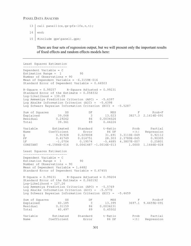
PANEL DATA ANALYSIS
301
13
14
15
call panel1(cs,qs~pfs~lfs,n,t);
end;
#include gpe\panel1.gpe;
There are four sets of regression output, but we will present only the important resultsof fixed effects and random effects models here:
Least Squares Estimation------------------------Dependent Variable = CEstimation Range = 1 90Number of Observations = 90Mean of Dependent Variable = -6.3159E-016Standard Error of Dependent Variable = 0.66503
R-Square = 0.99257 R-Square Adjusted = 0.99231Standard Error of the Estimate = 0.058332Log-Likelihood = 130.09Log Ammemiya Prediction Criterion (APC) = -5.6397Log Akaike Information Criterion (AIC) = -5.6398Log Schwarz Bayesian Information Criterion (BIC) = -5.5287
Sum of Squares SS DF MSS F Prob>FExplained 39.068 3 13.023 3827.3 2.1614E-091Residual 0.29262 86 0.0034026Total 39.361 89 0.44226
Variable Estimated Standard t-Ratio Prob PartialName Coefficient Error 86 DF >|t| RegressionQ 0.91928 0.029008 31.691 3.3110E-049 0.92112PF 0.41749 0.014751 28.303 2.3780E-045 0.90305LF -1.0704 0.19574 -5.4685 4.3807E-007 0.25801CONSTANT -6.1586E-016 0.0061487 -1.0016E-013 1.0000 1.1666E-028
Least Squares Estimation------------------------Dependent Variable = CEstimation Range = 1 90Number of Observations = 90Mean of Dependent Variable = 1.6482Standard Error of Dependent Variable = 0.67455
R-Square = 0.99231 R-Square Adjusted = 0.99204Standard Error of the Estimate = 0.060192Log-Likelihood = 127.26Log Ammemiya Prediction Criterion (APC) = -5.5769Log Akaike Information Criterion (AIC) = -5.5770Log Schwarz Bayesian Information Criterion (BIC) = -5.4659
Sum of Squares SS DF MSS F Prob>FExplained 40.185 3 13.395 3697.1 9.4659E-091Residual 0.31159 86 0.0036231Total 40.497 89 0.45502
Variable Estimated Standard t-Ratio Prob PartialName Coefficient Error 86 DF >|t| Regression

GAUSS PROGRAMMING FOR ECONOMETRICIANS AND FINANCIAL ANALYSTS
302
Q 0.90668 0.025625 35.383 4.9455E-053 0.93572PF 0.42278 0.014025 30.145 1.7169E-047 0.91354LF -1.0645 0.20007 -5.3206 8.1016E-007 0.24765CONSTANT 1.1873 0.025916 45.811 3.4012E-062 0.96064
The end of the estimation output produces a summary of the panel data analysis.Three sets of hypothesis testing for fixed and random effects are given. Based on theWald F-test and the Breusch-Pagan LM test, it is clear that there exist both fixedeffects and random effects for this model. Based on the Hausman specification test,however, there is no significant difference between the fixed and random effects.
Panel Data Model Estimation Procedure:(1) Pooled Regression(2) Between-Groups Regression(3) Fixed Effects (Within-Groups) Regression(4) Random Effects (Weighted Within-Groups) Regression
Wald F Test Statistic for No Fixed One-Way EffectsF( 5, 81) = 57.732
Breusch-Pagan LM Test Statistic for No One-Way EffectsChi-Sq( 1) = 334.85
Hausman's Test for Fixed and Randon EffectsChi-Sq( 3) = 0.75471
Within-Groups Estimates:Fixed S.E. Random S.E.
0.91928 0.029890 0.90668 0.0264040.41749 0.015199 0.42278 0.014451-1.0704 0.20169 -1.0645 0.20615
-6.1586e-016 0.0063356 1.1873 0.026704
One-Way Effects:Section/Period Fixed S.E. Random S.E.
1.0000 9.7059 0.19323 9.6378 0.183132.0000 9.6647 0.19908 9.5979 0.187163.0000 9.4970 0.22505 9.4408 0.206864.0000 9.8905 0.24185 9.7780 0.219185.0000 9.7300 0.26102 9.6299 0.233716.0000 9.7930 0.26374 9.6831 0.23544
Finally, within-groups estimates of the slope parameters and the individual interceptparameters are presented for the fixed effects and random effects models, respectively.Note that the estimated fixed effects, derived from the deviation approach, are thesame as those of dummy variables approach. Furthermore, the random effects aresimilar to the fixed effects, re-enforcing the result of the Hausman specification testthat there is no significant difference between the two models.

PANEL DATA ANALYSIS
303
Notice that the procedure panel1 is designed for study of individual (cross-section)effects. To study the time effects, swap the panel definition n and t and re-arrangethe stacked data series accordingly. For example, in Lesson 16.2, you can insert thefollowing statements (with comments for clarity) between line 10 and 11:
@ re-arrange data, then swap n and t @cs=vec(reshape(cs,n,t));qs=vec(reshape(qs,n,t));pfs=vec(reshape(pfs,n,t));lfs=vec(reshape(lfs,n,t));n=15;t=6;
We leave the estimation and interpretation of the time period effects as an exercise.
Once you understand and master the idea of one-way panel data analysis, it isstraightforward to extend it to two-way analysis. Both cross-section and time periodeffects are analyzed simultaneously under the respective assumptions of fixed effectsand random effects. Greene (1999) presented such extension as two exercises inChapter 14. We implement the two-way analysis in the module programPANEL2.GPE, which extends the module PANEL1.GPE for one-way analysis used inLesson 16.2. You may want to examine the code of PANEL2.GPE in comparison withthe outlined formula of Greene (1999), pp. 587-589. In essence, the two-way analysisruns five regressions: pooled regression, two between-groups (time periods and crosssections) regressions, and two within-groups (full deviations and partial deviations)regressions. From these regression estimations, we calculate overall, cross section, andtime period effects. As with one-way analysis, statistics for testing fixed effects,random effects, and for comparing fixed and random effects are computed. Themodule program PANEL2.GPE hides the details of implementation from all but themost curious eyes. PANEL2.GPE can be found in Appendix B-4 and it is installed inthe GPE sub-directory.
Lesson 16.3: Two-Way Panel Data Analysis
Extending the analysis of one-way effects, in this example we re-estimate the airlineservices production model to consider the two-way effects. We include PANEL2.GPEat the end of the program. Similar to the one-way analysis, two-way analysis is donewith the statement (see line 14 of Lesson 16.3 below):
call panel2(y,x,n,t);
where y, the dependent variable, and x, the independent variables, are stackedaccording to the panel definition of n blocks (cross sections) of t observations (timeperiods). The rest of the program for two-way analysis is identical as the previouslesson for one-way analysis.
/*

GAUSS PROGRAMMING FOR ECONOMETRICIANS AND FINANCIAL ANALYSTS
304
123456
7891011
1213
14
15
16
Lesson 16.3: Two-Way Panel Data AnalysisCost of Production for Airline Services III*/use gpe2;output file = gpe\output16.3 reset;load data[91,6] = gpe\airline.txt;panel = data[2:91,1:2]; @ panel definition @n=6;t=15;
/* stacked data series, by sections */cs = ln(data[2:91,3]); @ log cost (stacked) @qs = ln(data[2:91,4]); @ log output (stacked) @pfs = ln(data[2:91,5]); @ log fuel price (stacked) @lfs = data[2:91,6]; @ load factor (stacked) @xs = qs~pfs~lfs;
call reset;_names = "c","q","pf","lf";
call panel2(cs,xs,n,t);
end;
#include gpe\panel2.gpe;
It takes five regression estimations to carry out two-way panel data analysis. To savespace, we will report only the summary information as follows:
Panel Data Model Estimation Procedure:(1) Pooled Regression(2) Between-Groups (Cross Sections) Regression(3) Between-Groups (Time Periods) Regression(4) Fixed Effects (Within-Groups) Regression(5) Random Effects (Weighted Within-Groups) Regression
Wald F Test Statistic for No Fixed Two-Way EffectsF( 19, 67) = 23.102
Breusch-Pagan LM Test Statistic for No Two-Way EffectsChi-Sq( 2) = 336.40
Hausman's Test for Fixed and Randon EffectsChi-Sq( 3) = 183.54
Within-Groups Estimates:Fixed S.E. Random S.E.
0.81725 0.031851 0.90237 0.0297420.16861 0.16348 0.42418 0.016306-0.88281 0.26174 -1.0531 0.22948
6.1829e-016 0.0054155 1.0109 0.025968
Two-Way Effects:Fixed Random
Overall 12.667 1.0031
Cross Sections Effects:Sections Fixed Random

PANEL DATA ANALYSIS
305
1.0000 0.12833 7.93482.0000 0.065495 7.89333.0000 -0.18947 7.72924.0000 0.13425 8.07095.0000 -0.092650 7.91716.0000 -0.045956 7.9710
Time Periods Effects:Periods Fixed Random1.0000 -0.37402 -0.00230322.0000 -0.31932 0.000747653.0000 -0.27669 0.00305294.0000 -0.22304 0.00499015.0000 -0.15393 0.000448436.0000 -0.10809 -0.00130277.0000 -0.076864 -0.00116918.0000 -0.020733 -0.000157669.0000 0.047220 0.002591210.000 0.091728 -0.001819011.000 0.20731 -0.001837812.000 0.28547 0.0004746113.000 0.30138 0.002221314.000 0.30047 0.002799015.000 0.31911 0.0043389
From the two-way analysis, we can see that the model exhibits significant fixed effectsand random effects. The magnitude and the pattern of the two effects are different.From examining the “Time Periods Effects” in the output, we see that the fixed effectsare larger than the random effects. On the other hand, we see that for the “CrossSections Effects”, the magnitude of the random effects is greater than that of the fixedeffects.
Remember that to analyze one-way (time or individual) effects, PANEL1.GPEshould be included. PANEL2.GPE is used for analyzing two-way (time andindividual) effects.
Seemingly Unrelated Regression SystemThe classical panel data analysis investigates only the intercept difference acrossindividuals or time periods. Consider a more general specification of the model:
Yit = Xitβi + εit (i=1,2,...,N; t=1,2,...,T).
Let Yi = [Yi1,Yi2,...,YiT]', Xi = [Xi1,Xi2,...,XiT]', and εi = [εi1,εi2,...,εiT]'. The stacked Nequations (T observations each) system is Y = Xββββ + εεεε, or

GAUSS PROGRAMMING FOR ECONOMETRICIANS AND FINANCIAL ANALYSTS
306
Y1
Y2 …YN
=
X1 0 … 0
0 X2 … 0 … … … … 0 0 … XN
β + ε1
ε2 …εN
Notice that not only the intercept but also the slope terms of the estimated parametersare different across individuals. Of course, the restrictions of identical slope termsacross individuals may be imposed for direct comparison with the classical methods.The error structure of the model is summarized as follows:
E(εεεε) = 0E(Xεεεε) = 0E(εεεεεεεε') = Σ⊗ I
where Σ = [σij, i,j=1,2,...N] is the NxN variance-covariance matrix and I is a T×Tidentity matrix. Notice that contemporaneous correlation across individuals isassumed, although the assumption of no serial correlation is implied. The errorstructure of this model is different than that of the random effects model describedabove.
The system estimation techniques such as 3SLS and FIML should be used forparameter estimation in this kind of model, known as the Seemingly UnrelatedRegression Estimation (SUR) in the current context. The SUR estimation method wasdiscussed in Chapter XIII. Denote b and S as the estimated ββββ and Σ, respectively.Then,
b = [X'(S-1⊗ I)X]-1X'(S-1⊗ I)yVar(b) = [X'(S-1⊗ I)X]-1, andS = ee'/T, where e = y-Xb is the estimated error εεεε.
The advantage of the SUR estimation method for panel data analysis is that it not onlyallows the intercept difference between individuals (as in the fixed and random effectsmodels), but also allows the slope to vary among individuals. If the slope parametersare assumed to be constant across individuals, the method differs from the randomeffects model in the fundamental assumption of the covariance structure. By allowingcross-section correlation, the restricted SUR method is more general than the classicalrandom effects model.
Lesson 16.4: Panel Data Analysis for Investment Demand: Deviation Approach
To demonstrate the different approaches for panel data analysis, we consider thefollowing classical example of investment demand (Greene, 1999, Chap. 15; Grunfeldand Griliches, 1960; Boot and deWitt, 1960):

PANEL DATA ANALYSIS
307
Iit = αi + β1i Fit + β2i Cit + εit
Where i 5 firms: General Motors, Chrysler, General Electric,Westinghouse, and United Steel.
t 20 years: 1935-1954.Iit Gross investment.Fit Market value.Cit Value of the stock of plant and equipment.
The panel data of 20 years for 5 companies are available in 5 separate files, one foreach company. The data files used are: ifcgm.txt (General Motor), ifcch.txt(Chrysler), ifcge.txt (General Electric), ifcwe.txt (Westinghouse), ifcus.txt (UnitedSteel).
First we assume that β1i = β1 and β2i = β2 for all firms. In other words, we areestimating the restricted SUR model by assuming that the slope parameters do notvary across firms. To estimate and compare the fixed effects and random effects forthe model, the following program which is essentially the same as that of Lesson 16.2.Since the five company data sets are read in separately as time series, somemanipulation is necessary to convert them into a stacked vector of dependent variablesand a stacked matrix of independent variables (see lines 8 through 14 in Lesson 16.4below). The stacked data format is required in order to use the PANEL1.GPE moduleprogram.
12
345678910
1112
1314
1516
/*Lesson 16.4: Panel Data Analysis for Investment DemandDeviation Approach*/use gpe2;output file = gpe\output16.4 reset;
load gmc[21,4] = gpe\ifcgm.txt;load chc[21,4] = gpe\ifcch.txt;load gec[21,4] = gpe\ifcge.txt;load wec[21,4] = gpe\ifcwe.txt;load usc[21,4] = gpe\ifcus.txt;i=gmc[2:21,2]~chc[2:21,2]~gec[2:21,2]~wec[2:21,2]~usc[2:21,2];f=gmc[2:21,3]~chc[2:21,3]~gec[2:21,3]~wec[2:21,3]~usc[2:21,3];c=gmc[2:21,4]~chc[2:21,4]~gec[2:21,4]~wec[2:21,4]~usc[2:21,4];
n=5; @ 5 cross sections (firms) @t=20; @ 20 time periods (years) @
@ stacked data series, by firms @ys = vec(i);xs = vec(f)~vec(c);
call reset;_names="i","f","c";

GAUSS PROGRAMMING FOR ECONOMETRICIANS AND FINANCIAL ANALYSTS
308
17
18
19
call panel1(ys,xs,n,t);
end;
#include gpe\panel1.gpe;
As described earlier, using the module PANEL1.GPE to estimate the one-way fixedand random effects gives us four sets of regression output: the pooled regression,between-groups means regression, within-groups full deviations regression, andwithin-groups partial deviations regression. You should check the details of eachregression output. We present only the summary results of the analysis.
Panel Data Model Estimation Procedure:(1) Pooled Regression(2) Between-Groups Regression(3) Fixed Effects (Within-Groups) Regression(4) Random Effects (Weighted Within-Groups) Regression
Wald F Test Statistic for No Fixed One-Way EffectsF( 4, 93) = 58.956
Breusch-Pagan LM Test Statistic for No One-Way EffectsChi-Sq( 1) = 453.82
Hausman's Test for Fixed and Randon EffectsChi-Sq( 2) = 0.033043
Within-Groups Estimates:Fixed S.E. Random S.E.
0.10598 0.015891 0.10489 0.0151120.34666 0.024161 0.34602 0.024770
-1.6507e-014 6.9118 -8.8082 8.1293
One-Way Effects:Section/Period Fixed S.E. Random S.E.
1.0000 -76.067 66.886 -69.356 58.2342.0000 -29.374 19.814 -33.176 19.3763.0000 -242.17 33.321 -213.56 31.0284.0000 -57.899 19.703 -57.575 19.2635.0000 92.539 33.947 72.218 31.535
It is interesting to find the classical estimates of fixed effects and random effects aresimilar. This is consistent with the very small Hausman specification test statisticshown in the output.
Lesson 16.5: Panel Data Analysis for Investment Demand: SUR Method
By restricting β1i = β1 and β2i = β2 for all firms, the restricted SUR estimation methodis used in direct comparison with the classical methods of panel data analysis. InChapter XIII we implemented and estimated a system of linear demand equationsusing the SUR estimation method. The use of the input control variable _eq in

PANEL DATA ANALYSIS
309
estimating the simultaneous linear equations system was discussed in detail in ChapterXIII. In Chapter III we introduced the implementation of restricted least squares withthe use of input control variable _restr. Parameter restrictions across equations in alinear equations system were again discussed in Chapter XIII. You may want toreview these chapters and the relevant examples before working on this lesson.
In Lesson 16.5, the restricted SUR method is estimated using iterative three-stage leastsquares (_method=3). The result is the same as full information maximumlikelihood.
12
345678910
1112
13
14
15
16
171819
/*Lesson 16.5: Panel Data Analysis for Investment Demand FunctionSeemingly Unrelated Regression Estimation*/use gpe2;output file = gpe\output16.5 reset;
load gmc[21,4] = gpe\ifcgm.txt;load chc[21,4] = gpe\ifcch.txt;load gec[21,4] = gpe\ifcge.txt;load wec[21,4] = gpe\ifcwe.txt;load usc[21,4] = gpe\ifcus.txt;i=gmc[2:21,2]~chc[2:21,2]~gec[2:21,2]~wec[2:21,2]~usc[2:21,2];f=gmc[2:21,3]~chc[2:21,3]~gec[2:21,3]~wec[2:21,3]~usc[2:21,3];c=gmc[2:21,4]~chc[2:21,4]~gec[2:21,4]~wec[2:21,4]~usc[2:21,4];
yvar=i;xvar=f~c;
call reset;
_names="i-gm","i-ch","i-ge","i-we","i-us","f-gm","f-ch","f-ge","f-we","f-us","c-gm","c-ch","c-ge","c-we","c-us";
@ I I I I I F F F F F C C C C C 1@_eq = -1 0 0 0 0 1 0 0 0 0 1 0 0 0 0,
0 -1 0 0 0 0 1 0 0 0 0 1 0 0 0,0 0 -1 0 0 0 0 1 0 0 0 0 1 0 0,0 0 0 -1 0 0 0 0 1 0 0 0 0 1 0,0 0 0 0 -1 0 0 0 0 1 0 0 0 0 1;
@ F C|F C|F C|F C|F C|q @_restr = -1 0 1 0 0 0 0 0 0 0 0,
-1 0 0 0 1 0 0 0 0 0 0,-1 0 0 0 0 0 1 0 0 0 0,-1 0 0 0 0 0 0 0 1 0 0,0 -1 0 1 0 0 0 0 0 0 0,0 -1 0 0 0 1 0 0 0 0 0,0 -1 0 0 0 0 0 1 0 0 0,0 -1 0 0 0 0 0 0 0 1 0;
_iter=200;_method=3;call estimate(yvar,xvar);

GAUSS PROGRAMMING FOR ECONOMETRICIANS AND FINANCIAL ANALYSTS
310
20 end;
You should run the program to get the full report of the estimation results. The outputof the restricted SUR estimation is lengthy, but can be summarized as follows:
Simultaneous Linear Equations Estimation----------------------------------------Number of Endogenous Variables = 5Number of Predetermined Variables = 11Number of Stochastic Equations = 5Number of Observations = 20Estimation Range = 1 20
Three Stages Least Squares EstimationMaximum Number of Iterations = 200Tolerance = 0.001…System R-Square = 0.59471Log-Likelihood = -490.75300
Equation Variable Estimated AsymptoticName Name Coefficient Std Error t-RatioI-GM F-GM 0.033825 0.0063427 5.3330
C-GM 0.15536 0.016608 9.3541CONSTANT 360.69 51.871 6.9536
I-CH F-CH 0.033825 0.0063427 5.3330C-CH 0.15536 0.016608 9.3541CONSTANT 43.839 6.9344 6.3220
I-GE F-GE 0.033825 0.0063427 5.3330C-GE 0.15536 0.016608 9.3541CONSTANT -25.543 13.842 -1.8454
I-WE F-WE 0.033825 0.0063427 5.3330C-WE 0.15536 0.016608 9.3541CONSTANT 6.8931 4.7102 1.4634
I-US F-US 0.033825 0.0063427 5.3330C-US 0.15536 0.016608 9.3541CONSTANT 292.18 27.650 10.567
Asymptotic Variance-Covariance Matrix of EquationsI-GM 39110.I-CH 3359.9 575.64I-GE 312.36 -49.662 670.86I-WE 317.11 30.538 178.24 96.919I-US 9742.5 1695.0 919.47 622.51 12240.
I-GM I-CH I-GE I-WE I-US
To compare the fixed effects, random effects, and SUR method, the estimatedparameters of the investment function are tabled together. The individual effects forthree methods (under different covariance assumptions) are shown in the rows ofintercept terms for each firm. Numbers in parentheses are the estimated standarderrors.

PANEL DATA ANALYSIS
311
Fixed Effects Random Effects SUR MethodSlope F 0.10598 (0.01589) 0.10489 (0.01511) 0.033825 (0.006343)
C 0.34666 (0.02416) 0.34602 (0.02477) 0.15536 (0.01661)Intercept GM -76.067 (66.886) -69.356 (58.234) 360.69 (51.871)
CH -29.374 (19.814) -33.176 (19.376) 43.839 (6.9344)GE -242.17 (33.321) -213.56 (31.028) -25.543 (13.842)WE -57.899 (19.703) -57.575 (19.263) 6.8931 (4.7102)US 92.539 (33.947) 72.218 (31.535) 292.18 (27.650)
Although the estimates from the models of fixed effects and random effects aresimilar, the parameter estimates obtained from the SUR estimation method are quitedifferent. The impact of different covariance assumptions when estimating the modelis obvious. Since the SUR method is typically applied to estimating a model withvarying slope as well as intercept terms, we can easily estimate the unrestricted modelby removing (or commenting out) the restriction statement in line 16 of Lesson 16.5above. By comparing the results to those of the restricted model, the validity of theassumption of constant slopes may be tested. The following table presents thecomparison results of restricted and unrestricted estimates (standard errors are inparentheses). The large likelihood ratio statistic of the two models, calculated as2×[-459.092-(-490.753)] = 63.322, leads us to the conclusion that the slopeparameters are not the same across the five firms under consideration.
Eq. Variable Unrestricted Model Restricted ModelI-GM F 0.12195 (0.020243) 0.033825 (0.006343)
C 0.38945 (0.031852) 0.15536 (0.01661)Constant -173.04 (84.280) 360.69 (51.871)
I-CH F 0.067451 (0.017102) 0.033825 (0.006343)C 0.30507 (0.026067) 0.15536 (0.01661)Constant 2.3783 (11.631) 43.839 (6.9344)
I-GE F 0.037019 (0.01177) 0.033825 (0.006343)C 0.11695 (0.021731) 0.15536 (0.01661)Constant -16.376 (24.961) -25.543 (13.842)
I-WE F 0.053861 (0.010294) 0.033825 (0.006343)C 0.026469 (0.037038) 0.15536 (0.01661)Constant 4.4891 (6.0221) 6.8931 (4.7102)
I-US F 0.0886 (0.045278) 0.033825 (0.006343)C 0.3093 (0.11783) 0.15536 (0.01661)Constant 138.01 (94.608) 292.18 (27.650)
Log-Likelihood -459.092 -490.753
In summary, we have presented the classical methods of panel data analysis: fixedeffects and random effects. A more general SUR approach was introduced, whichallowed us to consider contemporaneous correlation across individuals, which the

GAUSS PROGRAMMING FOR ECONOMETRICIANS AND FINANCIAL ANALYSTS
312
classical methods ignore. Misspecification issues such as autocorrelation andheteroscedasticity in panel data are important. In Chapter X we discussed the problemof autocorrelation associated with time series, while heteroscedasticity in cross-sectional models was covered in Chapter IX. The combination of autocorrelation andheteroscedasticity is common in models for panel data. The treatment ofautocorrelation for time-period effects and heteroscedasticity for cross-section effectswould be an integrated and complicated application of this and the twoaforementioned chapters, which we will not discuss here.
XVIILeast Squares Prediction
The art of forecasting lies in building a practical model for the real world application,and in the preceding chapters, we have presented all the tools necessary to do so inGPE. This chapter introduces the few remaining GPE control variables dedicatedsolely to least squares prediction and time series forecasting.
Least squares prediction is nothing more than the extrapolation of the estimatedregression model from a set of historical observations into the unknown future. It isassumed that given the stable model structure, the future state is predictible from thereplication of history.
Predicting Economic GrowthIn this chapter, we will consider a “conventional wisdom” that the future state of theeconomy (measured in terms of real GDP growth) is predictable by an index called theComposite Economic Leading Indicator, which is assembled and updated monthly bythe U. S. Department of Commerce. The Indicator is a weighted average of 11 short-run economic factors, such as stock prices and average hours worked. It is oftenreported in the media that this Leading Indicator can predict the direction of theeconomy 3 to 9 months into the future.
The lessons in this chapter use the data file gdp96.txt. It consists of four variables:QUARTER (quarterly index), GDP (Gross Domestic Product in billions of dollars),PGDP (Implicit Price Deflator of GDP, 1996 = 100), and LEADING (CompositeEconomic Leading Indicator, 1987 = 100). We note that LEADING is the quarterlyaverage of the monthly series.
The target variable is the annual growth rate of real GDP. The following GAUSSstatements generate the required data series of GDP growth:
rgdp = 100*gdp./pgdp;growth = 100*(rgdp-lagn(rgdp,4))./lagn(rgdp,4);
First, Real Gross Domestic Product is expressed in billions of 1996 dollars. Then,GDP growth is measured as the annual percentage rate of change in real GDP fromthe same quarter last year. Although the causal relationship of the variablesLEADING and GROWTH is well grounded, we have to make sure that these twovariables are cointegrated. It turns out that both variables are stationary or I(0) process

GAUSS PROGRAMMING FOR ECONOMETRICIANS AND FINANCIAL ANALYSTS
314
and thus do not have unit roots. Moreover, the two variables are cointegrated. Weleave the details of the unit roots and cointegration tests of LEADING and GROWTHas exercises. See also Chapter XVI for a thorough review.
We are now ready to construct a working model suitable for short-run structuralestimation and prediction. Since forecasting is a time-sensitive business, we reservethe last four quarters of data for ex-post forecast evaluation. In other words, we aregoing to estimate the model using data through 1999, and see how well the modelpredicts real GDP growth in the last four quarters of 2000. We will need to construct aworking model not only for historical estimation but also for forecasting.
If the variable LEADING can actually predict GROWTH several quarters ahead, thena distributed lag structure must be specified. As a result of trial and error, we havefound that both the current and one-year (four quarters) lag of LEADING are useful inexplaining historical GROWTH. In addition, the momentum effect of GDP growth iscaptured with a lagged dependent variable. The model error is identified to be aMA(4) process. By construction, the explanatory variable LEADING is the quarterlyaverage of the monthly series. The specification of fourth order moving average forthe model error term should, therefore, not be surprising. Of course, this may not bethe only working specification of the model you can construct. Throughout this bookwe have given examples of model building. We leave the process of finding the bestmodel for forecasting to you. However, we emphasize the importance of using GPEvariables such as _pdl and _dlags to determine the short-run dynamics of themodel structure.
We now turn to new forecasting features of the GPE package. In GPE, the work ofleast squares prediction is done by a procedure called forecast. Forecasts arecomputed usually after the estimation of the model. Calling forecast is similar tocalling estimate. In calling forecast, you need to specify only the dependentand independent variables (in that order). The estimated parameters and the associatedcovariance matrix of the previously estimated model are used to compute the forecastsfor the same model. The alternative is that you may specifiy a vector of estimatedregression coefficients and the associated covariance matrix including those ofautocorrelated error structure if the model is so specified. The forecasting perioddefaults to begin one observation after the estimation period ends and continues to theend of the data series. If future observations of the dependent variable becomeavailable, ex-post forecast error statistics based on the results of least squaresprediction can be used for model evaluation.
If there are longer series of right-hand-side explanatory variables, ex-ante forecastscan be computed upon request. The GPE control variables _fbegin and _fend areused to specify the beginning and ending of the multiple steps ahead of forecasts. Inmost cases, ex-ante forecasting depends on scenario assumptions made regarding the

LEAST SQUARES PREDICTION
315
explanatory independent variables. If the composite economic leading indicator canpredict the economy three to nine months ahead as claimed, our model certainly canpoint out the direction of GROWTH about one year in advance of LEADING.Furthermore, by making scenario assumptions about the variable LEADING (forexample assuming no change in LEADING for the next year or so) we can predict thefuture value of GROWTH even further out on the horizon.
Lesson 17.1: Ex-Post Forecasts and Forecast Error Statistics
Here is the program predicting economic growth with the composite economic leadingindicator:
12
345678910
111213
141516
171819
2021
22
23
/*** Lesson 17.1: Ex-Post Forecasts and** Forecast Error Statistics*/use gpe2;output file = gpe\output17.1 reset;
n=169; @ 1959.1 to 2000.4 @load z[n,4] = gpe\gdp96.txt;gdp = z[2:n,2];pgdp = z[2:n,3];leading = z[2:n,4];rgdp = 100*gdp./pgdp;growth = 100*(rgdp-lagn(rgdp,4))./lagn(rgdp,4);xvar = leading~lagn(leading,4);
/* Model Estimation */call reset;_rstat=1;_dlags=1;/*_bgtest=4;_ebtest=4;_acf=12;_acf2=12;*/_arma=0,4;_iter=100;_method=5;
_begin=9; @ 1961Q1 @_end=164; @ 1999Q4 @call estimate(growth,xvar);
/* Forecasting */_fstat=1;_fplot=1;@ _dynamic=1; @call forecast(growth,xvar);
end;
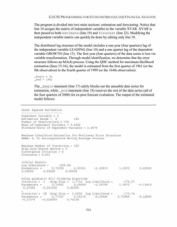
GAUSS PROGRAMMING FOR ECONOMETRICIANS AND FINANCIAL ANALYSTS
316
The program is divided into two main sections: estimation and forecasting. Notice thatline 10 assigns the matrix of independent variables to the variable XVAR. XVAR isthen passed to both estimate (line 19) and forecast (line 22). Modifying theindependent variable matrix can quickly be done by editing only line 10.
The distributed lag structure of the model includes a one-year (four quarters) lag ofthe independent variable LEADING (line 10) and a one quarter lag of the dependentvariable GROWTH (line 13). The first year (four quarters) of the data series is lost viavariable transformation. Through model identification, we determine that the errorstructure follows an MA(4) process. Using the QHC method for maximum likelihoodestimation (lines 15-16), the model is estimated from the first quarter of 1961 (or the9th observation) to the fourth quarter of 1999 (or the 164th observation):
_begin = 9;_end = 164;
The _begin statement (line 17) safely blocks out the unusable data series forestimation, while _end statement (line 18) reserves the rest of the data series (all ofthe four quarters of 2000) for ex-post forecast evaluation. The output of the estimatedmodel follows:
Least Squares Estimation------------------------Dependent Variable = YEstimation Range = 9 164Number of Observations = 156Mean of Dependent Variable = 3.4640Standard Error of Dependent Variable = 2.4074
Maximum Likelihood Estimation for Nonlinear Error StructureARMA( 0, 4) Autoregressive Moving Average Process
Maximum Number of Iterations = 100Step Size Search Method = 0Convergence Criterion = 0Tolerance = 0.001
Initial Result:Log Likelihood = -200.06Parameters = 0.72598 0.32261 -0.32815 1.0222 0.000000.00000 0.00000 0.00000
Using Quadratic Hill-Climbing AlgorithmIteration = 1 Step Size = 1.7716 Log Likelihood = -174.57Parameters = 0.75262 0.29208 -0.29795 1.0070 -0.13915-0.23366 -0.051020 0.62600…Iteration = 28 Step Size = 1.0000 Log Likelihood = -173.74Parameters = 0.77187 0.29116 -0.29460 0.72984 -0.12845-0.17370 -0.028399 0.70138

LEAST SQUARES PREDICTION
317
Final Result:Iterations = 28 Evaluations = 281112Log Likelihood = -173.74Parameters = 0.77187 0.29116 -0.29460 0.72984 -0.12845-0.17370 -0.028399 0.70138Gradient Vector = -0.029735 -0.75954 -0.74884 -0.0092271 -0.00032321 -0.00026542 -0.00020601 -0.00025569
Parameter Std.Error t-RatioMA( 1) -0.12845 0.075524 -1.7007MA( 2) -0.17370 0.074877 -2.3198MA( 3) -0.028399 0.080335 -0.35350MA( 4) 0.70138 0.076126 9.2134
NOTE: R-Square, AOV are computed from original series.
R-Square = 0.90568 R-Square Adjusted = 0.90382Standard Error of the Estimate = 0.74659Log-Likelihood = -173.74Log Ammemiya Prediction Criterion (APC) = -0.55915Log Akaike Information Criterion (AIC) = -0.55916Log Schwarz Bayesian Information Criterion (BIC) = -0.48096
Sum of Squares SS DF MSS F Prob>FExplained 851.19 3 283.73 509.02 4.8917E-079Residual 84.725 152 0.55740Total 898.31 155 5.7955
Variable Estimated Standard t-Ratio Prob PartialName Coefficient Error 152 DF >|t| RegressionY-1 0.77187 0.038674 19.958 2.5838E-044 0.72380X1 0.29116 0.034954 8.3299 1.0880E-014 0.31342X2 -0.29460 0.034512 -8.5361 0.00000 0.32404CONSTANT 0.72984 0.32619 2.2375 0.026708 0.031887
Squared Correlation of Observed and Predicted = 0.90615Sum of Squared Residuals = 84.725Sum of Absolute Residuals = 87.607Sum of Residuals = 8.18894E-001First-Order Rho = -0.018649Durbin-Watson Test Statistic = 1.9838Durbin-H Statistic = 0.11530
Although the estimated model with MA(4) error structure looks satisfactory, add thefollowing few lines before the estimation call (line 19):
_bgtest = 4;_ebtest = 4;_acf = 12;_acf2 = 12;
and re-run the model to verify the serial correlation problem in the conditional mean

GAUSS PROGRAMMING FOR ECONOMETRICIANS AND FINANCIAL ANALYSTS
318
and variance18, if any.
The next section of the program (lines 20 to 22), calls for least squares predictionbased on the estimated model. Simply calling forecast specifies the defaultprediction period, which begins after the last observation used in the regressionestimation, and ends with the end of the sample. We note that the beginning and endof the prediction period can be controlled by two GPE input variables, _fbegin and_fend, respectively.
In almost all cases, regression coefficients and the associated covariance matrix fromthe previously estimated model are used for prediction. The alternative is to set theforecast input variable named _b to the estimation output variable __b forspecifying the estimated regression parameters (and possibly including the estimatedparameters of the autocorrelated error structure). Similarly, for the purpose ofcomputing the variance of the forecasts, the estimated variance-covariance matrix__vb of the regression parameters must be used. Thus we set the forecast inputvariable _vb to the estimation output variable __vb. These are the requiredparameter information for the GPE procedure forecast (line 22) to carry out theforecasting task for an estimated model.
Ex-post forecast error statistics are computed by setting the input control variable_fstat=1 (line 20). This control variable is similar to its counterpart, _rstat,used for estimate. In addition, plotting of the forecasts and actuals can provide avisual clues as to the model’s performance. This is done in line 21 by setting the inputcontrol variable _fplot = 1.
Here is the forecast output:
Least Squares Prediction------------------------Dependent Variable = YPrediction Range = 165 168Using Regression Coefficients:
0.77187 0.29116 -0.29460 0.72984 -0.12845 -0.17370-0.028399 0.70138
Observation Observed Predicted Residual Std.Error165 5.29216 5.40534 -0.11318 0.75492166 6.09665 5.73282 0.36383 1.01130167 5.21095 5.19941 0.01154 1.20549168 3.41463 3.75958 -0.34495 1.31388
R-Square Between Observed and Predicted = 0.98040Mean Error (ME) = -0.020691
18 The dynamic model may be correlated in terms of conditional variance, identifiable withARCH or GARCH specification.

LEAST SQUARES PREDICTION
319
Mean Absolute Error (MAE) = 0.20837Mean Squared Error (MSE) = 0.066077Root Mean Squared Error (RMSE) = 0.25705Mean Absolute Percent Error (MAPE) = 4.6075Mean Squared Percent Error (MSPE) = 35.573Root Mean Squared Percent Error (RMSPE) = 5.9643Theil Inequality Coefficient = 0.025252Decomposition:Proportion Due to Bias = 0.0064791Proportion Due to Variance = 0.77294Proportion Due to Covariance = 0.22058Proportion Due to Regression = 0.70829Proportion Due to Disturbance = 0.28523
Each observation in the forecast period is listed, complete with observed andpredicted values. Residuals (or forecast errors) and their standard errors are alsogiven. Since we have put aside the last six quarters of the GROWTH data series to becompared with the forecasts, ex-post forecast error statistics, including Mean SquaredError and its components, are computed from the last six quarters of GDP growth.Moreover, forecasts in pairs with actuals are plotted together with the band of twostandard errors. We note that the upper and lower bounds of forecast are the minimalspread of the prediction. In reality, the forecast interval tends to be much wider due toadditional non-sampling errors. Econometrics texts describe the model evaluationbased on this set of forecast error statistics in detail. We leave judgment of themodel’s performance to you.
It can be shown that the method of least squares yields the best, linear, and unbiasedpredictor. Since the model is dynamic in nature (with a lagged dependent variable),we have an option to perform a dynamic forecast. A dynamic forecast is obtained byusing the predicted lagged dependent variable on the right-hand-side of theforecasting equation, instead of the actual lagged dependent variable. Let’s turn on thedynamic option of least squares prediction:
_dynamic = 1;
Make sure that the dynamic option is added before calling forecast, and run theprogram to see the result:
Least Squares Prediction------------------------Dependent Variable = YPrediction Range = 165 168Using Regression Coefficients:
0.77187 0.29116 -0.29460 0.72984 -0.12845 -0.17370-0.028399 0.70138
NOTE: Dynamic Prediction Computed.

GAUSS PROGRAMMING FOR ECONOMETRICIANS AND FINANCIAL ANALYSTS
320
Observation Observed Predicted Residual Std.Error165 5.29216 5.40534 -0.11318 0.75492166 6.09665 5.47912 0.61753 1.01065167 5.21095 4.15381 1.05715 1.20145168 3.41463 2.96447 0.45016 1.31095
R-Square Between Observed and Predicted = 0.83621Mean Error (ME) = 0.50292Mean Absolute Error (MAE) = 0.55950Mean Squared Error (MSE) = 0.42859Root Mean Squared Error (RMSE) = 0.65467Mean Absolute Percent Error (MAPE) = 11.434Mean Squared Percent Error (MSPE) = 173.13Root Mean Squared Percent Error (RMSPE) = 13.158Theil Inequality Coefficient = 0.067379Decomposition:Proportion Due to Bias = 0.59013Proportion Due to Variance = 0.0060607Proportion Due to Covariance = 0.40381Proportion Due to Regression = 0.042433Proportion Due to Disturbance = 0.36744
As expected, the model performance deteriorates when we forecast farther ahead intothe future. This is because the predicted value of the lagged dependent variable is usedin place of the actual value of the lagged dependent variable. Including the predictedvalue of the lagged dependent variable simply means that each forecast error iscompounded over the forecast period. One important characteristics of the dynamicforecast is that the further in the future we try to predict, the less reliable of theforecasts we get.
Lesson 17.2: Ex-Ante Forecasts
Forecasting is a time sensitive business. At the time of this writing, new informationon the Composite Economic Leading Indicator may become available. We couldmodify the data file gdp96.txt, or just add the new data into the program. The later isespecially helpful to carry out scenario ex-ante forecasts. That is, we extend the datafurther by making a scenario assumption about Leading Indicator to predict GDPgrowth in accordance with the assumption. For example, a “constant scenario” wouldassume no change (from the last year average) in the variable LEADING for the nextyear or so. Then, in line 7 of Lesson 17.2, the hypothesized observations ofLEADING are appended at the end of historical data series as follows:
leading = z[2:n,4]|108.8|108.8|108.8|108.8;
Recall that the variable z is the original data matrix read from the data file gdp96.txt.Similarly, we could create a “pessimistic scenario” similar to the following, in whichthe variable LEADING declines at 2 percent over the next year:
leading = z[2:n,4]|108.2|107.7|107.1|106.6;

LEAST SQUARES PREDICTION
321
Or, we could assume an “optimistic scenario” (2 percent annual growth rate) as well:
leading = z[2:n,4]|109.3|109.9|110.4|110.9;
In other words, ex-ante forecasts are nothing but a crystal-ball prediction aboutuncertain future conditions. To keep the model performance in line with the availableinformation, we do not use the dynamic features of the least squares prediction duringthe ex-post forecast periods. Dynamic forecast is automatic anyway, during the ex-ante forecast periods, since the value of the lagged dependent variable is not availableand must first be predicted for the period that follows.
The following program is almost identical to that of Lesson 17.1. Pay attention to thechange we made in line 7 assuming a scenario for ex-ante forecast:
12
3456
7
8910
111213141516171819
2021
22
23
/*** Lesson 17.2: Ex-Ante Forecasts*/use gpe2;output file = gpe\output17.2 reset;
n=169; @ 1951.1 to 2000.4 @load z[n,4] = gpe\gdp96.txt;gdp = z[2:n,2];pgdp = z[2:n,3];
/* pessimistic scenario (-2% AGR) */@ leading = z[2:n,4]|108.2|107.7|107.1|106.6; @/* constant scenario (0% AGR) */leading = z[2:n,4]|108.8|108.8|108.8|108.8;/* optimistic scenario (+2% AGR) */@ leading = z[2:n,4]|109.3|109.9|110.4|110.9; @
rgdp = 100*gdp./pgdp;growth = 100*(rgdp-lagn(rgdp,4))./lagn(rgdp,4);xvar = leading~lagn(leading,4);
/* Model Estimation */call reset;_rstat=1;_dlags=1;_arma=0,4;_iter=100;_method=5;_begin=9; @ 1961Q1 @_end=164; @ 1999Q4 @call estimate(growth,xvar);
/* Forecasting */_fstat=1;_fplot=1;@ _dynamic=1; @call forecast(growth,xvar);
end;

GAUSS PROGRAMMING FOR ECONOMETRICIANS AND FINANCIAL ANALYSTS
322
Here is the forecasting output of the “constant scenario”:
Least Squares Prediction------------------------Dependent Variable = YPrediction Range = 165 172Using Regression Coefficients:
0.77187 0.29116 -0.29460 0.72984 -0.12845 -0.17370-0.028399 0.70138
NOTE: Dynamic Prediction Computed.
Observation Observed Predicted Residual Std.Error165 5.29216 5.40534 -0.11318 0.75492166 6.09665 5.73282 0.36383 1.01130167 5.21095 5.19941 0.01154 1.20549168 3.41463 3.75958 -0.34495 1.31388169 2.52032 1.31668170 1.88011 1.31846171 1.52147 1.31970172 1.50094 1.32089
R-Square Between Observed and Predicted = 0.98040Mean Error (ME) = -0.020691Mean Absolute Error (MAE) = 0.20837Mean Squared Error (MSE) = 0.066077Root Mean Squared Error (RMSE) = 0.25705Mean Absolute Percent Error (MAPE) = 4.6075Mean Squared Percent Error (MSPE) = 35.573Root Mean Squared Percent Error (RMSPE) = 5.9643Theil Inequality Coefficient = 0.025252Decomposition:Proportion Due to Bias = 0.0064791Proportion Due to Variance = 0.77294Proportion Due to Covariance = 0.22058Proportion Due to Regression = 0.70829Proportion Due to Disturbance = 0.28523
Similarly, we run the other two scenarios, pessimistic (LEADING decreases) andoptimistic (LEADING increases), respectively. Instead of listing each of theforecasting results, we compare the respective ex-ante forecasts in the following table:
PredictedGDP Growth(%, annual rate)
Pessimistic (low)Scenario
ConstantScenario
Optimistic (high)Scenario
2001.1 2.35 2.52 2.672001.2 1.43 1.88 2.312001.3 0.68 1.52 2.322001.4 0.21 1.50 2.73

LEAST SQUARES PREDICTION
323
Furthermore, the following graph summaries the ex-post and ex-ante forecasts forthree different scenarios. The picture can tell a complicate story more clearly.
What you can say about the predictability of the Composite Economic LeadingIndicator? No matter which scenario is used the economy appears to be headingtowards a period of adjustment. Will the downward trend continue? Only under theoptimistic view, the economy could recover in the third quarter of 2001. It willcertainly depend on an effective government policy to revive the growth. Only timewill tell!


EpilogueThis is not the end of Gauss Programming for Econometricians andFinancial Analysts!
It is just the beginning. Many extensions of econometric estimation, testing, andforecasting techniques discussed in this book can be done with GPE. Takingadvantage of GPE output variables for each call to the main routine estimate orforecast, you can write add-on programs to do advanced applications as we didwith the GPE application modules in Appendix-B. Within the scope of econometricmodels we have discussed so far, you can experiment with the following extensions:
• Nonlinear ARCH-M Model Estimation and Prediction• Qualitative Choice Model with Heteroscedasticity• Panel Data Analysis with Heteroscedasticity and Autocorrelation
Many important topics in econometrics we did not cover here would certainly be goodcandidates for GAUSS implementation. To name a few examples:
• Monte Carlo Simulations and Bootstrapping Methods• Nonparametric Regression Analysis• Baysian Estimation and Inference• Benchmarking Econometric Computation
Beyond GPE, you may feel ready to write your own codes for econometric andstatistical applications. More than 400 GAUSS commands, procedures, and functionsare available at your disposal as part of the GAUSS programming environment. Wehave seen powerful procedures being developed over the past years. It is notunforeseeable that one day your research and programming skills may outgrow GPEand GAUSS.
If you are reaching far at this point, you will probably agree that learningeconometrics with GPE is certainly the right first step. We have demonstrated thatGAUSS is a programming environment built on the convenient syntax and operationsof matrix algebra. As you step through each lesson, learning to master GPE, you alsolearn GAUSS and econometrics. From here, the next step is up to you!


Appendix AGPE Control Variables
There are two types of global control variables in GPE: Input control variables andoutput control variables. For reference purpose, consider the following generalregression equation:
F(Z, β) = ε
Where Z is the data matrix of variables and β is the vector of parameters, which definethe functional form F. ε is the error structure of the model. Z can be furtherdecomposed as Z = [Y, X] with Y denoting the endogenous (dependent) variables andX the predetermined (independent) variables. If Y consists of more than one column,it is a system of linear equations. For a classical regression model, Y = f(X, β) + ε orF(Z, β) = Y - f(X, β) = ε. The simple case of single linear regression equation iswritten as:
Y = Xβ + ε
Where Y is the left-hand-side (LHS) or dependent variable, X is the right-hand-side(RHS) explanatory or independent variables. β is the vector of estimated parameters,and ε is the vector of estimated residuals.
Input Control VariablesInput control variables must be initialized before calling one of the main econometricroutines: estimate or forecast. To initialize all the global control variables, callreset will do it. That is,
call reset;
Three categories of input control variables are listed below: general-purpose inputcontrol variables, estimate input control variables, and forecast input controlvariables. Unless otherwise specified, setting each variable to 1 (that is, True or Yes)activates or turns on the optional behavior specified. If the variable is not defined orspecified, then its default value is assumed.

GAUSS PROGRAMMING FOR ECONOMETRICIANS AND FINANCIAL ANALYSTS
328
General Purpose Input Control Variables
Variable Description
_cmplx Complex number computation._cmplx = 0 (default): Do not allow for complex number computation,therefore negative argument for LN, LOG, and SQRT is not permitted;_cmplx =1: Allow for complex number computation.
_legend When a graph is requested (_rplot>0, see below),_legend = 1 (default): Shows legends for graph plots;_legend = 0: No legends will be shown.
_pause Pause the output before displaying graphs._pause = 0 (default): No waiting prompt;_pause = 1: Waiting for a keystroke to display graphs.
_print Controls screen output._print = 1 (default): Directs full output to screen;_print = 0: Directs partial output to screen. Verbose iteration outputsfrom a nonlinear or iterative model are suppressed;_print = -1: Suppress all screen output; Suppressing the screen outputwill force _rplot = 0 and _fplot = 0 (see below), but it will have no effecton sending output to a file or printer if requested.
ESTIMATE Input Control Variables
Variable Description
_acf Specify the number of lags for computing autocorrelation and partialautocorrelation coefficients from the estimated regression residuals.Useful for testing the ARMA error structure. Display and plot thefunctions if _rplot > 0 (see below). In addition, standard errors ofcoefficients and Box-Pierece and Ljung-Box portmanteau test statisticsare presented up to the number of lags specified in _acf. For example,12 lags of autocorrelation and partial autocorrelation functions arerequested by setting:_acf = 12;_acf = 0 (default).As an option of computing autocorrelation coefficients and theassociated standard errors using regression method, the second elementof the vector _acf may be set to a positive value, with the first element

APPENDIX A
329
indicating the number of lags requested. For example:_acf = 12,1;
_acf2 Same as _acf except that the autocorrelation and partial autocorrelationcoefficients are computed from the squared standardized residuals.Useful for testing the GARCH error structure._acf2 = 0 (default).
_ar Specify the order of an autoregressive (AR) error structure. If anadditional moving average process is desired for anautoregressivemoving average ARMA structure, use the variable _arma instead (seebelow). Optional initial values of the autocorrelation coefficients may beappended at the end of _ar for estimation. By providing the initial valuesis useful for starting search from non-zero values of autocorrelationcoefficients. For example:_ar = 1;_ar = 1, 0.5; @ with initial value of AR(1) parameter @_ar = 0 (default).
_arma Specify the orders of an autoregressive moving average (ARMA) errorstructure. It is a column vector consisting of at least two elements. Thefirst element denotes the order of autoregressive portion of the ARMAprocess, while the second element is the order of moving averageportion. If only the autoregressive portion is given, it is exactly the ARmodel (see _ar above). The model is estimated using maximumlikelihood method conditional to the initialization of pre-sample series,which is the sample mean of the error series. Optional initial values ofthe autoregressive and moving average coefficients may be appended atthe end of _arma for estimation. By giving the initial values is useful forstarting search from non-zero values of ARMA coefficients. Forexample:_arma = 1, 0; @ this is identical to: _ar = 1; @_arma = 0, 1;_arma = 1, 1, 0.5, -0.5; @ initial values of ARMA(1,1) parameters @_arma = 0, 0 (default).
_b A column vector of initial parameter values for nonlinear modelestimation.
_begin Specify the starting observation number for estimation._begin = 1 (default).
_bjtest Bera-Jarque test for residual normality._bjtest = 0 (default): Skip the test;

GAUSS PROGRAMMING FOR ECONOMETRICIANS AND FINANCIAL ANALYSTS
330
_bjtest = 1: Perform the test.
_bgtest Breusch-Godfrey test for higher order autocorrelation._bgtest = 0 (default): Skip the test;_bgtest = p (>0): Perform the test for autocorrelation up to the p-thorder. The number p (>0) is the highest order tested.
_bptest Breusch-Pagan and White tests for heteroscedasticity._bptest = 0 (default): Skip the test;_bptest = 1: Perform Breusch-Pagan and White tests for generalheteroscedasticity. For the Breusch-Pagan test, all explanatory variablesincluding constant term (i.e. X) are the RHS variables of the auxiliarytest regression. For the White test, all explanatory variables and theirsquares and cross product including constant term are the RHS variablesof the auxilary test regression.
_const Specify a constant term for a regression model._const = 1 (default): Constant term is added in the regression;_const = 0: No constant is added.
For a system model, this is a column vector of 0 (no constant) or 1 (withconstant) associated with each equation.
_conv Convergence criteria for nonlinear model estimation._conv = 0 (default): Convergence in function value and solution;_conv = 1: Convergence in function value, solution, and zero gradient.All convergence criteria are checked relative to the tolerance level _tol(see below).
_corr Compute condition number of explanatory variables and correlationmatrix of dependent and explanatory variables, useful formulticollinearity analysis._corr = 0 (default): Do not compute the statistics;_corr = 1: Compute and show the statistics.
_dlags A scalar or a 2x1 column vector to specify the use of lagged dependentvariables. As a scalar, it is the order of the regular lagged dependentvariables in use. As a 2x1 column vector, a seasonal lagged dependentvariables model is identified with order _dlags[1] and seasonal span_dlags[2] (require _dlags[2]>0). Normally, _dlags[2] = 4 for a modelwith quarterly data series, while _dlags[2] = 12 for monthly case._dlags[1] or the scalar _dlags is always the order number. For a pure(regular or seasonal) lagged dependent variables model, set RHSvariable X = 0 in calling ESTIMATE procedure and specify the column

APPENDIX A
331
vector _dlags accordingly. For example:_dlags = q; @ or equivalently, _dlags = q,1 @_dlags = q,s;Where q is the order of autocorrelation and s is the seasonal span._dlags = 0 (default).
For a system model, _dlags is a gxg matrix with the value of its entryindicating the number of lags for each endogenous variable (column) ineach equation (row). A zero ij-element of _dlags signifies that no lag isused for the j-th variable in the i-th equation. Here, g is the number ofendogenous variables or equations.
_drop Drop the first few observations for model estimation. Depending on themethod of estimation, initial unusable observations may be droppedautomatically._drop =1: Drops the first observation or the first seasonal span ofobservations for AR model estimation;_drop =0 (default): Keeps the first observation or the first seasonal spanof observations for AR model estimation with appropriate datatransformation.
_ebtest Engle-Bollerslev test for higher order autoregressive conditionalheteroscedasticity (ARCH)._ebtest = 0 (default): Skip the test;_ebtest = q (>0) :Perform the test for ARCH structure up to the q-thorder. The number q (>0) is the highest order tested.
_end Specify the ending observation number for estimation._end = rows(y) (default).
_eq Specify the stochastic equation specification matrix for system modelestimation. This is a gx(gs+ks) matrix with elements -1, 0, and 1arranged in accordance with the order of endogenous variables followedby the predetermined variables. Note that g is the number of stochasticequations. gs is the number of endogenous variables (gs>=g), while ks isthe number of predetermined variables. In the stochastic equationspecification matrix _eq, an element -1 indicates the LHS endogenousvariable. Only one -1 entry is allowed in each equation. An element 1indicates the use of an endogenous and/or a predetermined variable onthe RHS of an equation. An element 0 indicates the correspondingunused variable. If _eq is not specified, or _eq=0 by default, a seeminglyunrelated system is assumed. That is, g=gs and -1 in the gs diagonalsand 1 in the next gsxks predetermined variables portion of the matrix.

GAUSS PROGRAMMING FOR ECONOMETRICIANS AND FINANCIAL ANALYSTS
332
Normally constant terms are not included in the equation specification.
_garch Specify the orders of a generalized autoregressive conditonalheteroscedasticity (GARCH) error structure. It is a column vectorconsisting of at least two elements. The first element denotes the orderof autoregressive (variances) portion of GARCH process, while thesecond element is the order of moving average (squared errors) portion.The model is estimated using maximum likelihood method conditionalto the initialization of pre-sample series, which is the sample variance ofthe error series. The Optional initial value of GARCH coefficients maybe appended at the end of _garch for estimation. Be reminded that thereis always a constant for the GARCH process. The constant is the lastterm of GARCH parameters. By giving the initial values is useful forstarting search from non-zero values of GARCH coefficients. Forexample:_garch = 1, 0;_garch = 0, 1;_garch = 1, 1, 0.5, 0.5, 0.5; @ with initial values of GARCH(1,1) @_garch = 0, 0 (default).
_garchx Specify additional variables included in the GARCH variance equation(see _garch above). This may be a data matrix of multiple variables. Thevariables must be defined with the same number of rows or observationsas that of the regression residuals.
_hacv Compute heteroscedasticity and autocorrelation consistent variance-covariance matrix and perform adjustment to standard error and t-ratioof estimated coefficients accordingly. This may be a column vector up to3 elements._hacv = 0 (default): No adjustment;_hacv = 1: Compute heteroscedasticity consistent variance-covariancematrix;_hacv = 0,p: Compute p-th order autocorrelation consistent variance-covariance matrix with declining weights of autocovariances (Newey-West estimators), p=1,2,...;_hacv = 1,p: Compute heteroscedasticity and p-th orderautocorrelation consistent variance-covariance matrix with decliningweights of autocovariances (Newey-West estimators), p=1,2,....;_hacv = 1,p,1: Compute heteroscedasticity and p-th orderautocorrelation consistent variance-covariance matrix with the equalweighted autocovariances, p=1,2,....; Therefore, _hacv = 0,pis thesame as _hacv = 0,p,0 and _hacv = 1,pis the same as _hacv =1,p,0.

APPENDIX A
333
Note: If _hacv is used in conjunction with the instrumental variableestimation (see, _ivar below) and setting the number of iterations (see,_iter below) to achieve the convergence of estimated parameters, this isessentially the Generalized Method of Moments (GMM). _hacv ismeaningfully only when there is potential misspecification problem ofautoregressive and/or heteroscedastic error structure.
_hacv may be used in conjunction with the system model estimation. Ifthe method of 2SLS (see _method below) is requested with non-zero_hacv, then two stage GMM estimation is performed. Similarly, if themethod of 3SLS is requested with non-zero _hacv, then three stageGMM estimation is performed. However, the computed variance-covariance matrix for the system may become non-positive definite dueto excess numerical rounding errors or the improper autocovariancestructures specified.
_id Specify the identity equation specification matrix for a system model.Similar size and setup as _eq (see above) except that its entries can beany value as required. If _id is not specified, or _id=0 by default, there isno identity. Note: gs=rows(_eq|_id) to ensure the system compatibility.
_iter Maximum number of iterations requested for iterative or nonlinearmodel estimation._iter = 1 (default).
_ivar Instrumental variable estimation requested with instrumental variablesspecified in matrix _ivar. If _dlags[1] > 0, _ivar may be given with apositive scalar (i.e. _ivar = 1) and perform instrumental variableestimation with the internal instrumental variables obtained from theexplanatory variables and their lags. If the matrix form of _ivar isspecified, the external instrumental variables are used for thatcols(_ivar) >= cols(X) + _const and rows(_ivar) >= rows(X). Constantterm is automatically included in _ivar._ivar = 0 (default).
For a system model, external instrumental variable estimation may berequested with the instrumental variables specified in matrix _ivar. Thedata matrix _ivar will be combined with all predetermined variables toform the basis for instrumental variable estimation.
_ivar may be used togeter with _iter and _hacv (see above) to producethe GMM estimation.
_ma Specify the order of a moving average (MA) error structure. If an

GAUSS PROGRAMMING FOR ECONOMETRICIANS AND FINANCIAL ANALYSTS
334
additional autoregressive process is desired for anautoregressive movingaverage ARMA structure, use the variable _arma instead (see above).Optional initial values of the moving average coefficients may beappended at the end of _ma for estimation. By providing the initialvalues is useful for starting search from non-zero values of movingaverage coefficients. For example:_ma = 1;_ma = 1, 0.5; @ with initial value of MA(1) parameter @_ma = 0 (default).
_method Specify the estimation method for an AR model._method = 0 (default): Cochrane-Orcutt iterative LS method;_method = 0,1: Cochrane-Orcutt iterative ML method;method = 1: Beach-MacKinnon iterative ML method (for _ar=1 only,and _drop=0 is in effect);_method = 2 or 2,0: Hildreth-Lu grid search LS method (for _ar=1only);_method = 2,1: Hildreth-Lu grid search ML method (for _ar=1 only).Note: Higher AR order (_ar>1) can only use _method = 0 or method =0,1.
Specify the estimation method for a system model._method = 0 (default): Ordinary least squares (biased);_method = 1: Limited information maximum likelihood;_method = 2: Two-stage least squares;_method = 3: There-stage least squares;_method = 4: Full information maximum likelihood.Note: LIML and FIML are not true nonlinear maximum likelihoodestimation. Instead they are types of instrumental variables estimation.
Specify the estimation method for a nonlinear model (including a linearmodel with nonlinear error structure such as ARMA and GARCH)._method = 0 (default): Steep-ascent or decent method for mathematicaloptimization; Gauss-Newton method for nonlinear least squaresestimation; Berndt-Hall-Hall_Hausman (BHHH) method for maximumlikelihood estimation;_method = 1: Quasi-Newton BFGS update method;_method = 2: Quasi-Newton DFP update method;_method = 3: Greenstadt method;_method = 4: Newton-Raphson method;_method = 5: Quadratic hill-climbing method;_method = 6: Modified quadratic hill-climbing method.
_names Specify a vector of character names for variables (linear model) or

APPENDIX A
335
parameters (non-linear model) as appeared in a regression equation.
_nlopt Specify a nonlinear optimization problem._nlopt = 0 (default): Mathematical minimization of a scalar-valuedfunction or nonlinear least squares estimation based on a vector-valuedcomponent error function;_nlopt = 1: Mathematical maximization of a scalar-valued function ormaximum likelihood estimation based on a vector-valued componenterror function;_nlopt = 2 Maximum likelihood estimation based on a vector-valuedcomponent log-likelihood function.
_pdl Specify a polynomial distributed lag model if _pdl is defined as arows(_pdl)x3 matrix. Each row of _pdl consists three elements: q p rwhere q = lags, p = orders, and r = endpoint restrictions: -1 (beginning),1 (ending), 2 (both), and 0 (no restriction), for each RHS variable.Requires rows(_pdl) = cols(X), and cols(_pdl) = 3:_pdl = 0 (default).
_restart Number of times to restart estimation for iterative or nonlinear modelswhen function value does not improve. Maximum value of _restart is 10._restart = 0 (default).
_restr Perform restricted least squares estimation with the linear restrictionsdefined in accordance with the form: Rb = q, or [R1 R0][b1 b0]’ = q,where b1 is the vector of slope coefficients and R1 is the restrictionmatrix corresponds to b1. Similarly, b0 is the intercept and R0corresponds to b0. q is the vector of restricted values. Linear restrictionsinvolving intercept should be specified in conjunction with _const = 0. If_restr is specified, then _restr = [R1 q]. Requires rows(_restr) = numberof restrictions, and cols(_restr) = cols(X)._restr = 0 (default).
For a system model, restrictions in the matrix R are stacked horizontallyin accordance with the equations, while the vertical rows indicate thenumber of restrictions imposed. Own or cross equation restrictions canbe coded easily. In general restrictions on the constant terms are notrequired.
_rlist List regression residual series._rlist = 0 (default): Skip listing the series;_rlist = 1: List observed, predicted, and least squares residual series;_rlist = 2: In addition to list least squares residual series, studentizedresiduals and leverage information are provided. Useful for checking

GAUSS PROGRAMMING FOR ECONOMETRICIANS AND FINANCIAL ANALYSTS
336
influential observations and outliers.
_rplot Plot regression residual series._rplot = 0 (default): No plots;_rplot = 1: Plots residuals only;_rplot = 2: Plots both observed and predicted, and residuals.Also for plotting autocorrelation and partial autocorrelation functions ifrequested (see _acf above), a positive value of _rplot is needed.
_rstat Report regression residual statistics._rstat = 0 (default): Do not report the statistics;_rstat =1: Reports residual statistics, including DW, DH wheneverappropriate.
_step Specify step size of line search method for iterative or nonlinear modelestimation._step = 0 (default): Cut back (half) step size is used;_step = 1: Quadratic step size is used.
_tol Set the convergence tolerance level for iterative or nonlinear modelestimation._tol = 0.001 (default).
_vcov Report the estimated variance-covariance matrix._vcov = 0 (default): Do not report the variance-covariance matrix;_vcov = 1: Report variance-covariance matrix and correlation matrix ofthe estimated coefficients.
For a nonlinear model,_vcov = 1: Variance-covariance matrix is derived from the methoddependent approximated hessian (information matrix);_vcov = 2: Variance-covariance matrix is derived from the estimatedhessian._vcov = 3: Robust variance-covariance matrix, if available, is derivedfrom the maximum likelihood estimation of component error or log-likelihood function.
_weight Perform weighted least squares estimation with the weighting variabledefined in _weight. _weight must be a column vector androws(_weight) >= rows(X)._weight = 0 (default).

APPENDIX A
337
FORECAST Input Control Variables
In addition to the ESTIMATE input variables which control the model specification(e.g., _ar, _arma, _dlags, _pdl, etc.), the following are the FORECAST inputvariables:
Variable Description
_b Parameter estimates for computing the forecasts. Depending on themodel specification, it may include the estimated coefficients of AR orARMA error structures. Forecasting with GARCH innovations is notimplemented.
_dynamic Dynamic forecasts for lagged dependent variables model._dynamic = 0 (default): Do not perform dynamic forecasts;_dynamic = 1: Perform dynamic forecasts. Dynamic forecast usesprevious predicted lagged dependent variables.
_fbegin Start of forecast observation number._fbegin = _end +1 (default).
_fend End of forecast observation number._fend = rows(X) (default).
_fplot Plots predicted or forecast series._fplot = 0 (default): Do not plots the series;_fplot = 1: Plots predicted or forecast series.
_fstat Computes ex-post forecast error statistics._fstat = 0 (default): Do not compute the statistics._fstat = 1: Computes and report the statistics.
_unlog Computes unlogged series of forecasts._unlog = 0 (default): Do not computes unlogged series of forecasts;_unlog = 1: Computes unlogged series of forecasts, assuming the originalseries has been log transformed.
_vb Compute and report the estimated variance-covariance matrix of thebasic model (not including the variance-covariance matrix of AR orARMA error structure if specified).
Note: FORECAST is not available for nonlinear models.
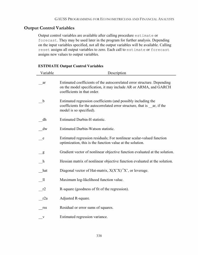
GAUSS PROGRAMMING FOR ECONOMETRICIANS AND FINANCIAL ANALYSTS
338
Output Control VariablesOutput control variables are available after calling procedure estimate orforecast. They may be used later in the program for further analysis. Dependingon the input variables specified, not all the output variables will be available. Callingreset assigns all output variables to zero. Each call to estimate or forecastassigns new values to output variables.
ESTIMATE Output Control Variables
Variable Description
__ar Estimated coefficients of the autocorrelated error structure. Dependingon the model specification, it may include AR or ARMA, and GARCHcoefficients in that order.
__b Estimated regression coefficients (and possibly including thecoefficients for the autocorrelated error structure, that is __ar, if themodel is so specified).
__dh Estimated Durbin-H statistic.
__dw Estimated Durbin-Watson statistic.
__e Estimated regression residuals; For nonlinear scalar-valued functionoptimization, this is the function value at the solution.
__g Gradient vector of nonlinear objective function evaluated at the solution.
__h Hessian matrix of nonlinear objective function evaluated at the solution.
__hat Diagonal vector of Hat-matrix, X(X’X)-1X’, or leverage.
__ll Maximum log-likelihood function value.
__r2 R-square (goodness of fit of the regression).
__r2a Adjusted R-square.
__rss Residual or error sums of squares.
__v Estimated regression variance.

APPENDIX A
339
FORECAST Output Control Variables
Variable Description
__f Predicted or forecast series.
__mape Mean absolute percent of forecast errors
__mse Mean sum squares of forecast errors
__rmspe Root mean absolute percent of forecast errors.
__u1 Theil inequality coefficient (0<=__u1<=1)
__uc Covariance proportion of mean sum squares of errors.
__ue Disturbance proportion of mean sum squares of errors.
__um Bias proportion of mean sum squares of errors.
__ur Regression proportion of mean sum squares of errors.
__us Variance proportion of mean sum squares of errors.
__vf Variance of predicted or forecast series.
Note: FORECAST is not available for nonlinear models.


Appendix B GPE Application Modules
Each of the GPE application modules is given AS IT IS. The user is free to use and tomake change as need for different purpose. However, the usual declaimer applies. Inparticular, the following copyright statement must be presented as long as all or partof the program code is used in your work.
(C) Copyright 2001 by Kuan-Pin Lin and Applied Data AssociatesAll Rights Reserved.
THIS SOFTWARE PRODUCT IS PROPRIETARY SOURCE CODE OF APPLIED DATAASSOCIATES. THIS FILE HEADER MUST ACCOMPANY ALL FILES USING ANY PORTION, INWHOLE OR IN PART, OF THIS SOURCE CODE. THIS SOFTWARE PRODUCT IS DESIGNED TOBE USED WITH GPE2 AND GAUSS. IF YOU USE THIS SOURCE CODE FOR RESEARCH ANDDEVELOPMENT, A PROPER REFERENCE IS REQUIRED. IF YOU WISH TO DISTRIBUTE ANYPORTION OF THE PROPRIETARY SOURCE CODE, IN WHOLE OR IN PART, YOU MUST FIRSTOBTAIN WRITTEN PERMISSION FROM THE AUTHOR.
Application Module B-1: GMM.GPE/*** GMM.GPE: Nonlinear GMM Estimation**** ==> call estimate(&gmmqw,x);** or** ==> call estimate(&gmmq,x);**** A set of moment functions must be defined as a procedure with the** name mf(x,b). The result is an nxl matrix of moments. n is the** number of sample observations; l is the number of moment equations;** x is the data matrix and b is the parameter vector.**** A global variable gmmw is used to define the weighting matrix for** the GMM criterion function (to be minimized). gmmw is initially** an identity matrix or 1 for the 1st GMM estimation; gmmw should be** set to gmmv(x,b), the inverse of the variance-covariance matrix of** moments functions, for the 2nd GMM estimation.**** gmmqw is the objective function with externally defined weighting** matrix gmmw, the result is a consistent GMM estimation.**** gmmq is the objective function with internally estimated weighting** matrix, the result is an efficient GMM estimation.**
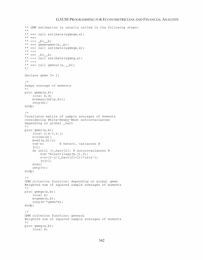
GAUSS PROGRAMMING FOR ECONOMETRICIANS AND FINANCIAL ANALYSTS
342
** GMM estimation is usually called in the following steps:**** ==> call estimate(&gmmqw,x);** ==>** ==> _b=__b;** ==> gmmw=gmmv(x,_b);** ==> call estimate(&gmmqw,x);** ==>** ==> _b=__b;** ==> call estimate(&gmmq,x);** ==>** ==> call gmmout(x,__b);*/
declare gmmw ?= 1;
/*Sampe average of moments*/proc gmmm(x,b);
local m,d;m=meanc(mf(x,b));retp(m);
endp;
/*Covariance matrix of sample averages of momentsconsidering White-Newey-West autocovariancesdepending on global _hacv*/proc gmmv(x,b);
local n,m,v,s,j;n=rows(x);m=mf(x,b)/n;v=m'm; @ hetero. variances @j=1;do until j>_hacv[2]; @ autocovariances @
s=m'*missrv(lagn(m,j),0);v=v+(1-j/(_hacv[2]+1))*(s+s');j=j+1;
endo;retp(v);
endp;
/*GMM criterion function: depending on global gmmwWeighted sum of squared sample averages of moments*/proc gmmqw(x,b);
local m;m=gmmm(x,b);retp(m'*gmmw*m);
endp;
/*GMM criterion function: generalWeighted sum of squared sample averages of moments*/proc gmmq(x,b);
local m;
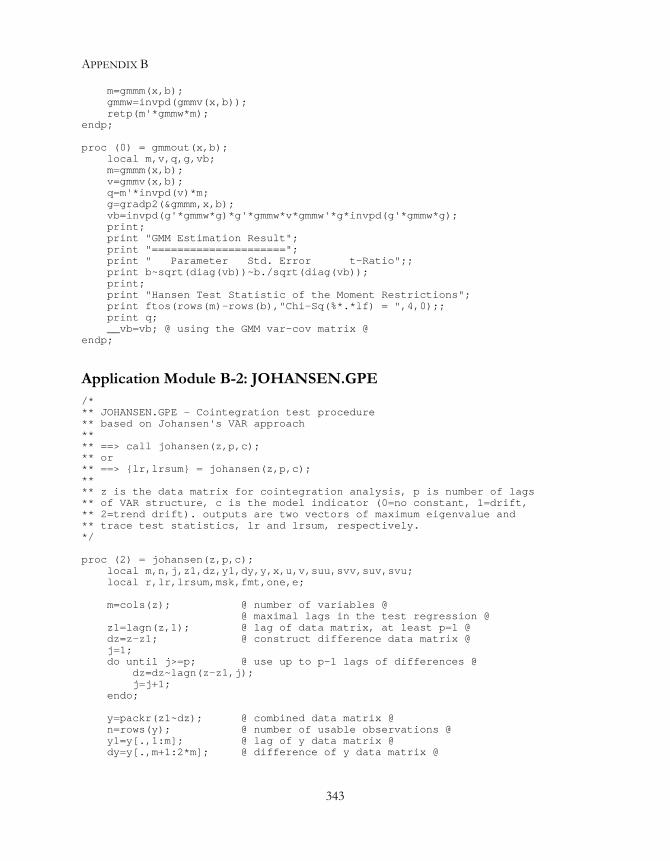
APPENDIX B
343
m=gmmm(x,b);gmmw=invpd(gmmv(x,b));retp(m'*gmmw*m);
endp;
proc (0) = gmmout(x,b);local m,v,q,g,vb;m=gmmm(x,b);v=gmmv(x,b);q=m'*invpd(v)*m;g=gradp2(&gmmm,x,b);vb=invpd(g'*gmmw*g)*g'*gmmw*v*gmmw'*g*invpd(g'*gmmw*g);print;print "GMM Estimation Result";print "=====================";print " Parameter Std. Error t-Ratio";;print b~sqrt(diag(vb))~b./sqrt(diag(vb));print;print "Hansen Test Statistic of the Moment Restrictions";print ftos(rows(m)-rows(b),"Chi-Sq(%*.*lf) = ",4,0);;print q;__vb=vb; @ using the GMM var-cov matrix @
endp;
Application Module B-2: JOHANSEN.GPE/*** JOHANSEN.GPE - Cointegration test procedure** based on Johansen's VAR approach**** ==> call johansen(z,p,c);** or** ==> lr,lrsum = johansen(z,p,c);**** z is the data matrix for cointegration analysis, p is number of lags** of VAR structure, c is the model indicator (0=no constant, 1=drift,** 2=trend drift). outputs are two vectors of maximum eigenvalue and** trace test statistics, lr and lrsum, respectively.*/
proc (2) = johansen(z,p,c);local m,n,j,z1,dz,y1,dy,y,x,u,v,suu,svv,suv,svu;local r,lr,lrsum,msk,fmt,one,e;
m=cols(z); @ number of variables @@ maximal lags in the test regression @
z1=lagn(z,1); @ lag of data matrix, at least p=1 @dz=z-z1; @ construct difference data matrix @j=1;do until j>=p; @ use up to p-1 lags of differences @
dz=dz~lagn(z-z1,j);j=j+1;
endo;
y=packr(z1~dz); @ combined data matrix @n=rows(y); @ number of usable observations @y1=y[.,1:m]; @ lag of y data matrix @dy=y[.,m+1:2*m]; @ difference of y data matrix @
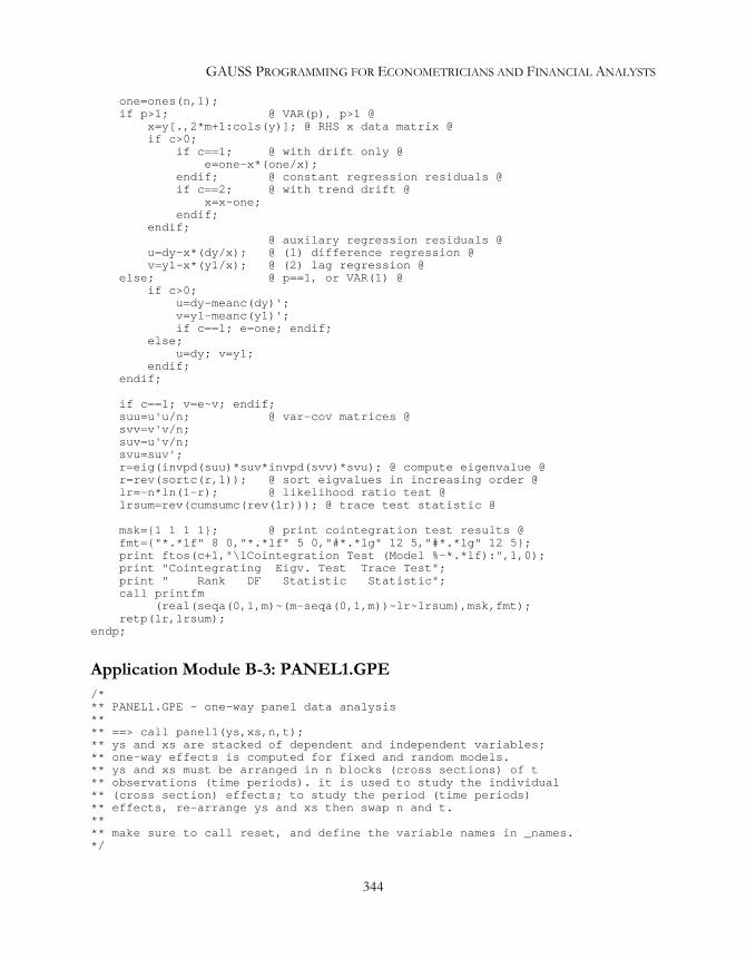
GAUSS PROGRAMMING FOR ECONOMETRICIANS AND FINANCIAL ANALYSTS
344
one=ones(n,1);if p>1; @ VAR(p), p>1 @
x=y[.,2*m+1:cols(y)]; @ RHS x data matrix @if c>0;
if c==1; @ with drift only @e=one-x*(one/x);
endif; @ constant regression residuals @if c==2; @ with trend drift @
x=x~one;endif;
endif;@ auxilary regression residuals @
u=dy-x*(dy/x); @ (1) difference regression @v=y1-x*(y1/x); @ (2) lag regression @
else; @ p==1, or VAR(1) @if c>0;
u=dy-meanc(dy)';v=y1-meanc(y1)';if c==1; e=one; endif;
else;u=dy; v=y1;
endif;endif;
if c==1; v=e~v; endif;suu=u'u/n; @ var-cov matrices @svv=v'v/n;suv=u'v/n;svu=suv';r=eig(invpd(suu)*suv*invpd(svv)*svu); @ compute eigenvalue @r=rev(sortc(r,1)); @ sort eigvalues in increasing order @lr=-n*ln(1-r); @ likelihood ratio test @lrsum=rev(cumsumc(rev(lr))); @ trace test statistic @
msk=1 1 1 1; @ print cointegration test results @fmt="*.*lf" 8 0,"*.*lf" 5 0,"#*.*lg" 12 5,"#*.*lg" 12 5;print ftos(c+1,"\lCointegration Test (Model %-*.*lf):",1,0);print "Cointegrating Eigv. Test Trace Test";print " Rank DF Statistic Statistic";call printfm
(real(seqa(0,1,m)~(m-seqa(0,1,m))~lr~lrsum),msk,fmt);retp(lr,lrsum);
endp;
Application Module B-3: PANEL1.GPE/*** PANEL1.GPE - one-way panel data analysis**** ==> call panel1(ys,xs,n,t);** ys and xs are stacked of dependent and independent variables;** one-way effects is computed for fixed and random models.** ys and xs must be arranged in n blocks (cross sections) of t** observations (time periods). it is used to study the individual** (cross section) effects; to study the period (time periods)** effects, re-arrange ys and xs then swap n and t.**** make sure to call reset, and define the variable names in _names.*/

APPENDIX B
345
proc (0) = panel1(ys,xs,n,t);local y,x,ym,xm,yms,xms,k;local rssr,rssur,dfr,dfur,bp,wf,v1,v,w,h;local b1,b2,vb1,vb2,a1,a2,va1,va2,xm1,xm2;
/* panel data processing */k=cols(xs);@ ys,xs: stacked data series @@ y,x: panel data series @y=reshape(ys,n,t)';x=reshape(vec(xs),n*k,t)';@ ym,xm: group means @ym=meanc(y);xm=reshape(meanc(x),k,n)';@ yms,xms: stacked group means @yms=vec(reshape(ym,t,n));xms=reshape(reshape(xm',k*t,n)',n*t,k);
/* pooled (restricted) regression */call estimate(ys,xs);rssr=__rss;dfr=__df;@ testing for random one-way effects @bp=(n*t/2)*(1/(t-1))*(
(sumc(sumc(reshape(__e,n,t)')^2)/sumc(sumc(__e^2))-1)^2);
/* between-group (mean) regression */call estimate(ym,xm);v1=t*__v;
/* within-group (mean deviation) regression */@ unrestricted regression @call estimate(ys-yms,xs-xms);rssur=__rss;dfur=__df-(n-1);v=__v*(__df/dfur); @ df adjusted variance @@ testing for fixed one-way effects @wf=((rssr-rssur)/(dfr-dfur))/(rssur/dfur);
/* fixed effects model */b1=__b;vb1=__vb*(__df/dfur);xm1=xm~(-ones(n,1));a1=ym-xm1*b1; @ section/period difference @va1=v/t+xm1*vb1*xm1';
/* random effects model */w=1-minc(sqrt(v/v1)|1);@ if w==1, it is fixed effects model @@ if w==0, it is a pooled model (no effects) @call estimate(ys-w*yms,xs-w*xms);b2=__b;vb2=__vb*(__df/dfur);if w>0;
xm2=xm~((-1/w)*ones(n,1));a2=w*(ym-xm2*b2);va2=(w^2)*(v/t+xm2*vb2*xm2');
else;a2=zeros(n,1);

GAUSS PROGRAMMING FOR ECONOMETRICIANS AND FINANCIAL ANALYSTS
346
va2=zeros(n,n);endif;h=(b1[1:k]-b2[1:k])'*inv(vb1[1:k,1:k]-vb2[1:k,1:k])*(b1[1:k]-b2[1:k]);
/* print output */print;print "Panel Data Model Estimation Procedure:";print "(1) Pooled Regression";print "(2) Between-Groups Regression";print "(3) Fixed Effects (Within-Groups) Regression";print "(4) Random Effects (Weighted Within-Groups) Regression";print;print "Wald F Test Statistic for No Fixed One-Way Effects";print ftos(dfr-dfur,"F(%*.*f,",4,0);;print ftos(dfur,"%*.*f) = ",4,0);;print wf;print;print "Breusch-Pagan LM Test Statistic for No One-Way Effects";print ftos(1,"Chi-Sq(%*.*f) = ",4,0);;print bp;print;print "Hausman's Test for Fixed and Randon Effects";print ftos(k,"Chi-Sq(%*.*f) = ",4,0);;print abs(h);print;print "Within-Groups Estimates:";print " Fixed S.E. Random S.E.";;print b1~sqrt(diag(vb1))~b2~sqrt(diag(vb2));print;print "One-Way Effects:";print "Section/Period Fixed S.E. Random S.E.";;print seqa(1,1,n)~a1~sqrt(diag(va1))~a2~sqrt(diag(va2));
endp;
Application Module B-4: PANEL2.GPE/*** PANEL2.GPE - two-way panel data analysis**** ==> call panel2(ys,xs,n,t);** ys and xs are stacked of dependent and independent variables;** two-way effects is computed for fixed and random models.** ys and xs must be arranged in n blocks (cross sections) of t** observations (time periods).**** make sure to call reset, and define the variable names in _names.*/
proc (0) = panel2(ys,xs,n,t);local ymi,xmi,ymis,xmis,ystar,xstar,k;local ymt,xmt,ymts,xmts,ymm,xmm,y,x;local rssr,rssur,dfr,dfur,bp,wf,v1,v2,v3,v,w1,w2,w3,h;local b1,b2,vb1,vb2,a1i,a1t,a2i,a2t,c1,c2;
/* panel data processing (complicated, do not change) */k=cols(xs);@ ys,xs: stacked data series @@ y,x: panel data series @y=reshape(ys,n,t)';

APPENDIX B
347
x=reshape(xs',n*k,t)';@ xt=reshape(xs,n,k*t); @
@ ymi,xmi: cross section means @ymi=meanc(y);xmi=reshape(meanc(x),k,n)';@ ymt,xmt: time period means @ymt=meanc(y');@ xmt=reshape(meanc(xt),t,k); @xmt=reshape(meanc(reshape(xs,n,k*t)),t,k);
@ ymm,xmm: overall means @ymm=meanc(ymi)';xmm=meanc(xmi)';
@ ymis,xmis: stacked section means @ymis=vec(reshape(ymi,t,n));xmis=reshape(reshape(xmi',k*t,n)',n*t,k);@ ymts,xmts: stacked time period means @ymts=reshape(ymt,n*t,1);xmts=reshape(xmt,n*t,k);
/* pooled (restricted) regression */call estimate(ys,xs);rssr=__rss;dfr=__df;
@ testing for two-way effects @bp=(n*t/2)*((1/(t-1))*((sumc(sumc(reshape(__e,n,t)')^2)/sumc(sumc(__e^2))-1)^2)+(1/(n-1))*((sumc(sumc(reshape(__e,n,t))^2)/sumc(sumc(__e^2))-1)^2));
@ between-groups (cross sections) means regression @call estimate(ymi,xmi);v1=t*__v;
@ between-groups (time periods) means regression @call estimate(ymt,xmt);v2=n*__v;
/* fixed effects model */@ within-groups (cross sections and time periods) regression @ystar=ys-ymis-ymts+ymm;xstar=xs-xmis-xmts+xmm;call estimate(ystar,xstar);rssur=__rss;dfur=__df-(n-1)-(t-1); @ adust df @v=__v*(__df/dfur);
@ testing for fixed two-way effects @wf=((rssr-rssur)/(dfr-dfur))/(rssur/dfur);
b1=__b;vb1=__vb*(__df/dfur);c1=ymm-xmm*b1[1:k]; @ overall effects, note: b1[k+1]=0 @a1i=(ymi-ymm)-(xmi-xmm)*b1[1:k]; @ cross sections effects @a1t=(ymt-ymm)-(xmt-xmm)*b1[1:k]; @ time periods effects @
/* random effects model */v3=v1+v2-v;

GAUSS PROGRAMMING FOR ECONOMETRICIANS AND FINANCIAL ANALYSTS
348
w1=1-minc(sqrt(v/v1)|1);w2=1-minc(sqrt(v/v2)|1);w3=w1+w2-(1-minc(sqrt(v/v3)|1));ystar=ys-w1*ymis-w2*ymts+w3*ymm;xstar=xs-w1*xmis-w2*xmts+w3*xmm;call estimate(ystar,xstar);
b2=__b;vb2=__vb*(__df/dfur);c2=w3*((ymm-xmm)*b2[1:k])+b2[k+1]; @ overall effect @a2i=(w1*ymi-w3*ymm)-(w1*xmi-w3*xmm)*b2[1:k]; @ individual effects @a2t=(w2*ymt-w3*ymm)-(w2*xmt-w3*xmm)*b2[1:k]; @ period effects @h=(b1[1:k]-b2[1:k])'*inv(vb1[1:k,1:k]-vb2[1:k,1:k])*(b1[1:k]-b2[1:k]);
/* print output */print;print "Panel Data Model Estimation Procedure:";print "(1) Pooled Regression";print "(2) Between-Groups (Cross Sections) Regression";print "(3) Between-Groups (Time Periods) Regression";print "(4) Fixed Effects (Within-Groups) Regression";print "(5) Random Effects (Weighted Within-Groups) Regression";print;print "Wald F Test Statistic for No Fixed Two-Way Effects";print ftos(dfr-dfur,"F(%*.*f,",4,0);;print ftos(dfur,"%*.*f) = ",4,0);;print wf;print;print "Breusch-Pagan LM Test Statistic for No Two-Way Effects";print ftos(2,"Chi-Sq(%*.*f) = ",4,0);;print bp;print;print "Hausman's Test for Fixed and Randon Effects";print ftos(k,"Chi-Sq(%*.*f) = ",4,0);;print abs(h);print;print "Within-Groups Estimates:";print " Fixed S.E. Random S.E.";;print b1~sqrt(diag(vb1))~b2~sqrt(diag(vb2));print;print "Two-Way Effects:";print " Fixed Random";print " Overall " c1~c2;print;print "Cross Sections Effects:";print " Sections Fixed Random";;print seqa(1,1,n)~a1i~a2i;print;print "Time Periods Effects:";print " Periods Fixed Random";;print seqa(1,1,t)~a1t~a2t;
endp;

Appendix C Statistical Tables
Statistical tables for normal distribution, t distribution, Chi-squared distribution, and Fdistribution are available from most of statistics references. Durbin-Watson boundstest statistics are readily available in econometric textbooks. In this Appendix, we listonly the not-so-popular statistical tables for testing unit roots and cointegrationdiscussed in Chapter XVI.
Table C-1. Critical Values for the Dickey-Fuller Unit Root TestBased on t-Statistic
Model
Model I: ∆Xt = (ρ-1) Xt-1 + Σi=1,2,…
ρi ∆Xt-i + εt
Model II: ∆Xt = α + (ρ-1) Xt-1 + Σi=1,2,…
ρi ∆Xt-i + εt
Model III: ∆Xt = α + β t + (ρ-1) Xt-1 + Σi=1,2,…
ρi ∆Xt-i + εt
Test Statistic
τρ t-statistic (non-symmetric distribution, testing ρ = 1)τα t-statistic (symmetric distribution, testing α = 0 given ρ = 1)τβ t-statistic (symmetric distribution, testing β = 0 given ρ = 1)
Source
Fuller (1976, p. 373); Dickey and Fuller (1981).

GAUSS PROGRAMMING FOR ECONOMETRICIANS AND FINANCIAL ANALYSTS
350
Model Statistic N 1% 2.5% 5% 10%I ττττρρρρ 25 -2.66 -2.26 -1.95 -1.60
50 -2.62 -2.25 -1.95 -1.61100 -2.60 -2.24 -1.95 -1.61250 -2.58 -2.23 -1.95 -1.61500 -2.58 -2.23 -1.95 -1.61>500 -2.58 -2.23 -1.95 -1.61
II ττττρρρρ 25 -3.75 -3.33 -3.00 -2.6250 -3.58 -3.22 -2.93 -2.60100 -3.51 -3.17 -2.89 -2.58250 -3.46 -3.14 -2.88 -2.57500 -3.44 -3.13 -2.87 -2.57>500 -3.43 -3.12 -2.86 -2.57
III ττττρρρρ 25 -4.38 -3.95 -3.60 -3.2450 -4.15 -3.80 -3.50 -3.18100 -4.04 -3.73 -3.45 -3.15250 -3.99 -3.69 -3.43 -3.13500 -3.98 -3.68 -3.42 -3.13>500 -3.96 -3.66 -3.41 -3.12
II τττταααα 25 3.41 2.97 2.61 2.2050 3.28 2,89 2.56 2.18100 3.22 2.86 2.54 2.17250 3.19 2.84 2.53 2.16500 3.18 2.83 2.52 2.16>500 3.18 2.83 2.52 2.16
III τττταααα 25 4.05 3.59 3.20 2.7750 3.87 3.47 3.14 2.75100 3.78 3.42 3.11 2.73250 3.74 3.39 3.09 2.73500 3.72 3.38 3.08 2.72>500 3.71 3.38 3.08 2.72
III ττττββββ 25 3.74 3.25 2.85 2.3950 3.60 3.18 2.81 2.38100 3.53 3.14 2.79 2.38250 3.49 3.12 2.79 2.38500 3.48 3.11 2.78 2.38>500 3.46 3.11 2.78 2.38

APPENDIX C
351
Table C-2. Critical Values for the Dickey-Fuller Unit Root TestBased on F-Statistic
Model
Model II: ∆Xt = α + (ρ-1) Xt-1 + Σi=1,2,…
ρi ∆Xt-i + εt
Model III: ∆Xt = α + β t + (ρ-1) Xt-1 + Σi=1,2,…
ρi ∆Xt-i + εt
Test Statistic
φ1 F-statistic (testing α = 0 and ρ = 1 on Model II)φ2 F-statistic (testing α = 0, β = 0, and ρ = 1 on Model III)φ3 F-statistic (testing β = 0 and ρ = 1 on Model III)
Source
Dickey and Fuller (1981).
Model Statistic N 1% 2.5% 5% 10%II φφφφ1 25 7.88 6.30 5.18 4.12
50 7.06 5.80 4.86 3.94100 6.70 5.57 4.71 3.86250 6.52 5.45 4.63 3.81500 6.47 5.41 4.61 3.79>500 6.43 5.38 4.59 3.78
III φφφφ2 25 8.21 6.75 5.68 4.6750 7.02 5.94 5.13 4.31100 6.50 5.59 4.88 4.16250 6.22 5.40 4.75 4.07500 6.15 5.35 4.71 4.05>500 6.09 5.31 4.68 4.03
III φφφφ3 25 10.61 8.65 7.24 5.9150 9.31 7.81 6.73 5.61100 8.73 7.44 6.49 5.47250 8.43 7.25 6.34 5.39500 8.34 7.20 6.30 5.36>500 8.27 7.16 6.25 5.34

GAUSS PROGRAMMING FOR ECONOMETRICIANS AND FINANCIAL ANALYSTS
352
Table C-3. Critical Values for the Dickey-Fuller Cointegrationt-Statistic ττττρρρρ Applied on Regression Residuals
Model
Yt = α + Xt β + εt
∆εt = (ρ-1) εt-1 + Σi=1,2,…ρi∆εt-i + utK = Numbers of variables in the cointegration tests, i.e. [Yt, Xt].t = 1,2,…,N (500).
Model 2: E(Yt) = E(Xt) = 0 (both X and Y have no drift).Model 2a: E(Xt) ≠ 0 (at least one variable in X has drift).Model 3: E(Yt) ≠ 0 but E(Xt) = 0 (only Y has drift).
Test Statistic
τρ t-statistic (testing ρ = 1)
Source
Phillips and Ouliaris (1990).
Model K 1% 2.5% 5% 10%2 2 -3.96 -3.64 -3.37 -3.07
3 -4.31 -4.02 -3.77 -3.454 -4.73 -4.37 -4.11 -3.835 -5.07 -4.71 -4.45 -4.166 -5.28 -4.98 -4.71 -4.43
2a 2 -3.98 -3.68 -3.42 -3.133 -4.36 -4.07 -3.80 -3.524 -4.65 -4.39 -4.16 -3.845 -5.04 -4.77 -4.49 -4.206 -5.36 -5.02 -4.74 -4.467 -5.58 -5.31 -5.03 -4.73
3 2 -4.36 -4.07 -3.80 -3.523 -4.65 -4.39 -4.16 -3.844 -5.04 -4.77 -4.49 -4.205 -5.36 -5.02 -4.74 -4.466 -5.58 -5.31 -5.03 -4.73
Note: For the case of two variables in Model 2a, X is trended but Y is not. It isasymptotically equivalent to ADF Unit Root Test for Model III (see Table C-1, τρ forN=500). If only Y has drift (Model 3), the cointegration equation can be expressed asYt = α + γ t + Xt β + εt. Therefore, the same critical values of Model 2a apply toModel 3 for one extra variable t (but not count for K).

APPENDIX C
353
Table C-4. Critical Values for Unit Root and Cointegration TestsBased on Response Surface Estimates
Critical values for unit root and cointegration tests can be computed from theequation:
CV(K, Model, N, e) = b + b1 (1/N) + b2 (1/N)2
Notation
Model: 1=no constant; 2=no trend; 3=with trend;K: Number of variables in cointegration tests (K=1 for unit root test);N: Number of observations or sample size;e: Level of significance, 0.01, 0.05, 0.1.
Source
MacKinnon (1991).

GAUSS PROGRAMMING FOR ECONOMETRICIANS AND FINANCIAL ANALYSTS
354
K Model e b b1 b21 1 0.01 -2.5658 -1.960 -10.041 1 0.05 -1.9393 -0.398 0.001 1 0.10 -1.6156 -0.181 0.001 2 0.01 -3.4335 -5.999 -29.251 2 0.05 -2.8621 -2.738 -8.361 2 0.10 -2.5671 -1.438 -4.481 3 0.01 -3.9638 -8.353 -47.441 3 0.05 -3.4126 -4.039 -17.831 3 0.10 -3.1279 -2.418 -7.582 2 0.01 -3.9001 -10.534 -30.032 2 0.05 -3.3377 -5.967 -8.982 2 0.10 -3.0462 -4.069 -5.732 3 0.01 -4.3266 -15.531 -34.032 3 0.05 -3.7809 -9.421 -15.062 3 0.10 -3.4959 -7.203 -4.013 2 0.01 -4.2981 -13.790 -46.373 2 0.05 -3.7429 -8.352 -13.413 2 0.10 -3.4518 -6.241 -2.793 3 0.01 -4.6676 -18.492 -49.353 3 0.05 -4.1193 -12.024 -13.133 3 0.10 -3.8344 -9.188 -4.854 2 0.01 -4.6493 -17.188 -59.204 2 0.05 -4.1000 -10.745 -21.574 2 0.10 -3.8110 -8.317 -5.194 3 0.01 -4.9695 -22.504 -50.224 3 0.05 -4.4294 -14.501 -19.544 3 0.10 -4.1474 -11.165 -9.885 2 0.01 -4.9587 -22.140 -37.295 2 0.05 -4.4185 -13.461 -21.165 2 0.10 -4.1327 -10.638 -5.485 3 0.01 -5.2497 -26.606 -49.565 3 0.05 -4.7154 -17.432 -16.505 3 0.10 -4.4345 -13.654 -5.776 2 0.01 -5.2400 -26.278 -41.656 2 0.05 -4.7048 -17.120 -11.176 2 0.10 -4.4242 -13.347 0.006 3 0.01 -5.5127 -30.735 -52.506 3 0.05 -4.9767 -20.883 -9.056 3 0.10 -4.6999 -16.445 0.00

APPENDIX C
355
Table C-5: Critical Values for the Johansen's Cointegration LikelihoodRatio Test Statistics
Notations
VAR Model: 1=no constant; 2=drift; 3=trend driftN: Sample Size, 400M: Number of Variablesr: Number of Cointegrating Vectors or RankDegree of Freedom = M-r
Source
Johansen (1988), Johansen and Juselius (1990), and Osterwald-Lenum (1992).
Model M-r 1% 2.5% 5% 10% 20% 50%
λλλλmax 1 1 6.51 4.93 3.84 2.86 1.82 0.581 2 15.69 13.27 11.44 9.52 7.58 4.831 3 22.99 20.02 17.89 15.59 13.31 9.711 4 28.82 26.14 23.80 21.58 18.97 14.941 5 35.17 32.51 30.04 27.62 24.83 20.162 1 11.576 9.658 8.083 6.691 4.905 2.4152 2 18.782 16.403 14.595 12.783 10.666 7.4742 3 26.154 23.362 21.279 18.959 16.521 12.7072 4 32.616 29.599 27.341 24.917 22.341 17.8752 5 38.858 35.700 33.262 30.818 27.953 23.1323 1 6.936 5.332 3.962 2.816 1.699 0.4473 2 17.936 15.810 14.036 12.099 10.125 6.8523 3 25.521 23.002 20.778 18.697 16.324 12.3813 4 31.943 29.335 27.169 24.712 22.113 17.7193 5 38.341 35.546 33.178 30.774 27.899 23.211
λλλλtrace 1 1 6.51 4.93 3.84 2.86 1.82 0.581 2 16.31 14.43 12.53 10.47 8.45 5.421 3 29.75 26.64 24.31 21.63 18.83 14.301 4 45.58 42.30 39.89 36.58 33.16 27.101 5 66.52 62.91 59.46 55.44 51.13 43.792 1 11.576 9.658 8.083 6.691 4.905 2.4152 2 21.962 19.611 17.844 15.583 13.038 9.3552 3 37.291 34.062 31.256 28.436 25.445 20.1882 4 55.551 51.801 48.419 45.248 41.623 34.8732 5 77.911 73.031 69.977 65.956 61.566 53.3733 1 6.936 5.332 3.962 2.816 1.699 0.4473 2 19.310 17.299 15.197 13.338 11.164 7.6383 3 35.397 32.313 29.509 26.791 23.868 18.7593 4 53.792 50.424 47.181 43.964 40.250 33.6723 5 76.955 72.140 68.905 65.063 60.215 52.588


ReferencesGAUSS for Windows User Guide (Version 3.5), 2000, Aptech Systems, Inc.GAUSS Language Reference (Version 3.5), 2000, Aptech Systems, Inc.
E. Berndt and D. Wood, 1975, “Technology, Prices, and the Derived Demand forEnergy,” Review of Economics and Statistics, 259-268.
T. Bollerslev, 1986, "Generalized Autoregressive Conditional Heteroskedasticity,"Journal of Econometrics 31, 307-327.
T. Bollerslev and E. Ghysels, 1996, "Periodic Autoregressive ConditionalHeteroscedasticity," American Statistical Association Journal of Business andEconomic Statistics, 14, 139-151.
J. Boot and G. deWitt, 1960, “Investment Demand: An Empirical Contribution to theAggregation Problem,” International Economic Review, 1, 3-30.
J. Y. Campbell, A. W. Lo, and A. C. Mackinlay, 1977, The Econometrics of FinancialMarkets, Princeton University Press.
R. Davidson and J. G. MacKinnon, 1973, Estimation and Inference in Econometrics,Oxford University Press.
D. A. Dickey and W. A. Fuller, 1981, “Likelihood Ratio Statistics for AutoregressiveTime Series with a Unit Root,” Econometrica, 49, 1057-1072.
P. J. Dhrymes, 1970, Econometrics, Harper & Row, New York.R. Engle and C. Granger, 1987, “Co-integration and Error Correction: Representation,
Estimation and Testing,” Econometrica, 35, 251-276.R. F. Engle, 1982, "Autoregressive Conditional Heteroscedasticity with Estimates of
the Variance of United Kingdom Inflation," Econometrica, 50, 987-1006.R. F. Engle, D. M. Lilien, and R. P. Robins, 1987, "Estimating Time-Varying Risk
Premia in the Term Structure: the ARCH-M Model," Econometrica 55, 391-407.R. Fair, 1978, “A Theory of Extramarital Affairs,” Journal of Political Economy, 86,
45-61.W. A. Fuller, 1976, Introduction to Statistical Time Series, John Wiley, New York.S. Goldfeld and R. Quandt, 1972, Nonlinear Methods in Econometrics, Chapter 1:
Numerical Optimization, North-Holland, 1-38.W. H. Greene, 1999, Econometric Analysis, 4th ed., Prentice Hall.W. H. Greene, 1997, Econometric Analysis, 3rd ed., Prentice Hall.Y. Grunfeld and Z. Griliches, 1960, “Is Aggregation Necessarily Bad?” Review of
Economics and Statistics, 42, 1-13.A. Hall, 1993, "Some Aspects of Generalized Method of Moments Estimation,"
Handbook of Statistics, Vol. 11, ed. by G. S. Maddala, C. R. Rao, and H. D.Vinod, Elsevier Science Publishers, North-Holland, 393-417.
R. Hall, 1978, “Stochastic Implications of the Life Cycle-Permanent IncomeHypothesis: Theory and Evidence,” Journal of Political Economy 86, 971-987.

GAUSS PROGRAMMING FOR ECONOMETRICIANS AND FINANCIAL ANALYSTS
358
J. D. Hamilton, 1994, Time Series Analysis, Princeton University Press.L. P. Hansen and K. J. Singleton, 1982, "Generalized Instrumental Variables
Estimation of Nonlinear Rational Expectations Models," Econometrica 50, 1269-1286.
J. Hausman, 1975, “An Instrumental Variable Approach to Full-InformationEstimators for Linear and Certain Nonlinear Models,” Econometrica, 727-738.
F. Hayashi, 2000, Econometrics, Princeton University Press.S. Johansen, 1988, “Statistical Analysis of Cointegration Vectors,” Journal of
Economic Dynamics and Control, 12, 231-254.S. Johansen and K. Juselius, 1990, “Maximum Likelihood Estimation and Inference
on Cointegration with Applications to the Demand for Money,” Oxford Bulletin ofEconomics and Statistics, 52, 169-210.
G. G. Judge, R. C. Hill, W. E. Griffiths, H. Lutkempohl, and T.-C. Lee, 1988,Introduction to the Theory and Practice of Econometrics, 2nd ed., John Wiley andSons.
G. G. Judge, R. C. Hill, W. E. Griffiths, and T.-C. Lee, 1985, Theory and practice ofEconometrics, 2nd ed., John Wiley and Sons.
L. Klein, 1950, Economic Fluctuations in the United States: 1921-1941, John Wileyand Sons.
J. G. MacKinnon, 1991, “Critical Values for Cointegration Tests,” in Long-RunEconomic Relationships: Readings in Cointegration, ed. by R. F. Engle and G. W.Granger, Oxford University Press, 267-276.
T. C. Mills, 1999, The Econometric Modeling of Financial Time Series, 2nd ed.,Cambridge University Press.
R. C. Mittelhammer, G. G. Judge, and D. J. Miller, 2000, Econometric Foundations,Cambridge University Press.
D. B Nelson, 1991, “Conditional Heteroscedasticity in Asset Returns, A NewApproach,” Econometrica, 59, 347-370.
D. B Nelson and C. Q. Cao, 1992, “Inequality Constraints in the Univariate GARCHModel,” Journal of Business and Economic Statistics, 10, 229-235.
M. Ogaki, 1993, "Generalized Method of Moments: Econometric Applications,"Handbook of Statistics, Vol. 11, ed. by G. S. Maddala, C. R. Rao, and H. D.Vinod, Elsevier Science Publishers, North-Holland, 455-488.
M. Osterwald-Lenum, 1992, “A Note with Quantiles of the Asymptotic Distribution ofthe Maximum Likelihhod Cointegration Rank Test Statistics,” Oxford Bulletin ofEconomics and Statistics, 54, 461-471.
P. C. B. Phillips and S. Ouliaris, 1990, “Asymptotic Properties of Residual BasedTests for Cointegration,” Econometrica, 58, 165-193.
R. E. Quandt, 1983, “Computational Problem and Methods,” Handbook ofEconometrics, Vol. I, ed. by Z. Griliches and M. D. Intriligator, Chapter 12, 699-764, North-Holland.
L. Spector and M. Mazzeo, 1980, “Probit Analysis and Economic Education,”Journal of Economic Education, 11, 37-44.

359
Index
Analysis of variance, AOV, 54Analytical derivatives, 98Analytical Jacobian, 124ARCH in mean, ARCH-M, 281ARMA analysis for regression residuals,
277ARMAX regression model, 277Augmented Dickey-Fuller (ADF) test, 249Autocorrelation, 163
Beach-MacKinnon iterative maximumlikelihood method, 172
Box-Pierce Q test, 168, 177Breusch-Godfrey LM test, 168, 177Durbin-H test, 194Durbin-Watson bounds test, 167first order, AR(1), 167higher order, 176Hildreth-Lu grid search method, 171Ljung-Box Q test, 168, 177Prais-Winsten modified Cochrane-
Orcutt method, 171Autocorrelation coefficient, 168, 272Autocorrelation function, ACF, 169, 271,
281Autocorrelation-consistent covariance
matrix, 164Autoregressive conditional
heteroscedasticity, ARCH, 271Box-Pierce Q test, 281Engle-Bollerslev LM test, 281Ljung-Box Q test, 281
Autoregressive moving average, ARMA,180, 271Box-Pierce Q test, 272Breusch-Godfrey LM test, 274, 281Durbin-Watson bound test, 274Ljung-Box Q test, 272
Berndt-Wood model, 236Binary choice model, 135Box-Cox variable transformation, 121, 132
Censored regression model. See Limiteddependent variable model
CES production function, 110, 118, 129Cobb-Douglas production function, 60, 79,
185Coefficient of relative risk aversion, 218Cointegrating rank, 259Cointegrating vector, 259Cointegration test, 250
Engle-Granger test, 260Johansen test, 263maximal eigenvalue test statistic, 266trace test statistic, 266
Composite economic leading indicator,313
Concentrated log-likelihood function, 113,122, 243
Constant returns to scale, CRS, 60Correlation matrix, 57, 86
Data generating process, DGP, 249Dickey-Fuller (DF) test, 249Distributed lag models, 193
Almon lag, 193autoregressive distributed lag, ARDL,
193, 203geometric lag, 193Koyck lag, 193lagged dependent variable, 193polynomial lag, 193, 200
Dummy variable, 73, 135additive, 73, 79multiplicative, 73, 79
Dummy variable trap, 74, 78

GAUSS PROGRAMMING FOR ECONOMETRICIANS AND FINANCIAL ANALYSTS
360
Economies of scale, 294Elasticity, 62, 123
long-run, 193short-run, 193
Elasticity of subsititution, 238Error correction model, 260Euler equation, 217
Forecasting, 313dynamic forecast, 319ex-ante forecast, 314ex-post forecast, 314forecast error statistics, 314
Full information maximum likelihood,FIML, 227
Gamma probability distribution, 102, 207,210
GAUSS, 5array operation, 15built-in functions or procedures, 30characteristic roots or eigenvalues, 35characteristic vectors or eigenvectors,
35condition number, 36cumulative distribution function, 37data transformation, 24descriptive statistics, 37element-by-element compatibility, 17file input and output, 24gradient, 37hessian, 37least squares solution, 35logical operator, 20matrix operation, 15probability density function, 36publication quality graphics, 44relational operator, 18sequential quadratic programming, 37
GAUSS for Windows, 5active file, 21Command window, 6Debug window, 7Edit window, 6
GAUSS library system, 47main file, 21main file list, 21Output window, 6
Generalized autoregressive conditionalheteroscedasticity, GARCH, 280
Generalized method of momentsHansen test for moment restrictions, 209Langrangian multiplier test, 217Likelihood ratio test, 217linear model, 222nonlinear model, 210quadratic criterion function, 208Wald test, 217White-Newey-West estimator, 208
Generalized method of moments, GMM,207
Global control variables, 48, 327input control variables, 48output control variables, 48
Goodness of fit, R2, adjusted R2, 54GPE package, 5, 48
Heteroscedasticity, 149Breusch-Pagan test, 155Goldfeld-Quandt test, 153Koenkar-Basset test, 156maximum likelihood estimation, 158weighted least squares, 152White test, 155
Heteroscedasticity-autocorrelation-consistent covariance matrix, 163, 212
Heteroscedasticity-consistent covariancematrix, 150, 163, 212
Hypothesis testings in nonlinear modelsLagrangian multiplier test, LM test, 128Likelihood ratio test, LR test, 129
Hypothesis testings in nonlinear models,127Wald test, 128
Information matrix, 102Input control variable, 327
_acf, 169, 176, 181, 274

361
_acf2, 281_ar, 171, 180, 276, 277_arma, 180, 276_b, 96, 318_begin, 66, 155, 233, 316_bgtest, 169, 176, 181, 274_bjtest, 69, 156_const, 63, 79, 235_conv, 99, 180_corr, 86_dlags, 194, 204, 233, 267_drop, 171_dynamic, 319_ebtest, 281_end, 66, 155, 316_eq, 226, 308_fbegin, 318_fend, 318_fplot, 318_fstat, 318_garch, 282_garchx, 283_hacv, 150, 165, 212, 222_id, 226_iter, 171, 222, 230_ivar, 197, 222, 227_jacob, 120, 125_method, 99, 172, 226_names, 53_nlopt, 96, 121, 138, 146, 180_pdl, 200, 204_print, 111, 174_restart, 100, 160, 232_restr, 62, 76, 82, 201, 235, 253, 308_rlist, 56, 69_rplot, 56, 233_rstat, 55, 194, 233_step, 99_tol, 99, 175, 232_vb, 318_vcov, 57, 109, 150, 230_weight, 155
Instrumental variable, 197, 222
Instrumental variable estimation, IV, 193,215
Jacobian, 244Jacobian transformation, 119
Klein Model I, 227
L’Hôspital’s rule, 122Latent variable, 136Least squares estimation, 48Least squares prediction, 48. See
ForecastingLikelihood function, 102Limited dependent variable model, 135Limited information maximum likelihood,
LIML, 227Linear probability model, 136Linear restriction, 62, 235
Wald F-test, 64, 77Logistic curve, 136Logit model, 136Log-likelihood function, 102, 119, 138,
144, 243Log-normal probability distribution, 102Longitudinal data, 291
Maximum likelihood estimation, 99, 119Moment function, 207Moment restrictions, 209Moving average, 180Multicollinearity, 85
condition number, 36, 86Theil’s measure, 88variance inflation factors, VIF, 90
Multiple regression, 57Multiplicative heteroscedasticity, 159
Newey-West estimator, 163Nonlinear full information maximum
likelihood, 242Nonlinear least squares, 99, 117Nonlinear optimization, 95
BFGS quasi-Newton method, 99
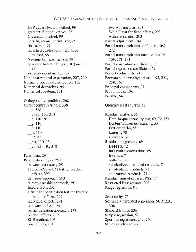
GAUSS PROGRAMMING FOR ECONOMETRICIANS AND FINANCIAL ANALYSTS
362
DFP quasi-Newton method, 99gradient, first derivatives, 95Greenstadt method, 99hessian, second derivatives, 95line search, 99modified quadratic-hill climbing
method, 99Newton-Raphson method, 99quadratic hill-climbing (QHC) method,
99steepest-ascent method, 99
Nonlinear rational expectation, 207, 219Normal probability distribution, 102Numerical derivatives, 95Numerical Jacobian, 121
Orthogonality condition, 208Output control variable, 338
__a, 318__b, 93, 110, 318__e, 110, 261__g, 110__h, 110__ll, 110__r2, 88__rss, 110, 154__vb, 93, 110, 318
Panel data, 291Panel data analysis, 291
between-estimates, 293Breusch-Pagan LM test for random
effects, 299deviation approach, 293dummy variable approach, 292fixed effects, 292Hausman specification test for fixed or
random effects, 299individual effects, 291one-way analysis, 291partial deviation approach, 298random effects, 299SUR method, 306time effects, 291
two-way analysis, 303Wald F-test for fixed effects, 293within-estimates, 293
Partial adjustment, 194Partial autocorrelation coefficient, 168,
272Partial autocorrelation function, PACF,
169, 271, 281Partial correlation coefficient, 85Partial regression coefficient, 59Perfect collinearity, 74Permanent income hypothesis, 193, 223,
259, 263Principal components, 91Probit model, 136P-value, 54
Qrdinary least squares, 51
Residual analysis, 55Bera-Jarque normality test, 69, 70, 156Durbin-Watson test statistic, 55first-order rho, 55kurtosis, 70skewness, 70
Residual diagnostics, 69DFFITS, 72influential observations, 69leverage, 71outliers, 69standardized predicted residuals, 71standardized residuals, 71studentized residuals, 71
Residual sum of squares, RSS, 64Restricted least squares, 308Ridge regression, 91
Seasonality, 73Seemingly unrelated regression, SUR, 226,
306Shepard lemma, 236Simple regression, 52Spurious regression, 249, 260Structural change, 65

363
Chow test, 65dummy variable approach, 79
Sum-of-squares, 95, 111System of simultaneous equations, 225
endogenous variable, 225identity equation, 226predetermined variable, 225stochastic equation, 226
Three-stage least squares, 3SLS, 227Time series analysis, 271
serial correlation in the mean, 271serial correlation in the variance, 271
Time series conversion, 43, 46
Tobit analysis, 144Transfer function. See ARMAX regression
modelTranslog cost function, 236t-ratio, 54Two-stage least squares, 2SLS, 227
Unconstrained optimization, 95Unit roots test, 249
Variance-covariance matrix, 57, 109, 127,152, 164, 209
Weighted least squares, 126


ELECTRONIC MEDIA TRANSMITTAL AND GAUSS LightTM SOFTWARETerms and Conditions of Use for the CD-ROM Accompanying
COMPUTATIONAL ECONOMETRICSGAUSS Programming for Econometricians and Financial Analysts
NOTICE: DO NOT UNSEAL THE ENVELOPE ENCLOSING THE CD-ROM (MEDIA) ORUSE THE MEDIA OR ITS CONTENTS BEFORE READING THESE TERMS ANDCONDITIONS OF USE. PUBLISHER AUTHORIZES USE OF THE MEDIA ANDCONTENTS ONLY UNDER THESE TERMS AND CONDITIONS OF USE. IFRECIPIENT DOES NOT WISH TO BE BOUND BY THESE TERMS AND CONDITIONSOF USE, RECIPIENT IS PROHIBITED FROM USING THE MEDIA AND CONTENTS,AND RECIPIENT SHALL RETURN THE MEDIA AND CONTENTS TO PUBLISHER.RECIPIENT'S UNSEALING OF THE ENVELOPE AND/OR USE OF THE MEDIA ORCONTENTS SIGNIFIES RECIPIENT'S AGREEMENT TO THESE TERMS ANDCONDITIONS OF USE.
1. ACCEPTANCE OF TERMS. Recipient's unsealing of the envelope enclosing the Media andContents or use of the Media or Contents subjects Recipient to all terms and conditions of usedescribed in this document and also all terms and conditions of the GAUSS LightTM Licensedisplayed in the Media. Publisher and Aptech authorize use of the Media and Contents only asset forth herein and within the GAUSS LightTM License.
2. NO WARRANTIES: Publisher and Aptech do not warrant the accuracy of the Contents ascontained in the Media against data corruption, computer viruses, errors in file transfer data,unauthorized revisions to the files, or any other alterations or data destruction to the file(s).The Media and its Contents are transmitted as is. Publisher and Aptech shall not have anyliability for Recipient's use of the Media or its Contents, including without limitation, anytransmittal of bugs, viruses, or other destructive or harmful programs, scripts, aplets or files tothe computers or networks of the Recipient. Recipient acknowledges and agrees that Recipientis fully informed of the possibility of the Media or its Contents being harmful to Recipientscomputers or networks and the possibility that the Contents may not be an exact and virus-freecopy of masters by Publisher or Aptech. Recipient also acknowledges, agrees and warrants thatRecipient shall be solely responsible for inspection and testing of the Media and the Contentsfor bugs, viruses, or other destructive or harmful programs, scripts, aplets or files, beforeacessing or using the Media or Contents.
3. NO IMPLIED WARRANTIES. THERE ARE NO IMPLIED WARRANTIES,INCLUDING WARRANTIES OF MERCHANTABILITY OR FITNESS FOR APARTICULAR PURPOSE, WITH RESPECT EITHER TO THE MEDIA OR THECONTENTS.
4. LIMITATIONS ON LIABILITY AND REMEDIES. Publisher and Aptech shall have noliability for any general damages, direct or indirect damages, special damages, exemplary

damages, statutory damages, punitive damages, or consequential damages, including withoutlimitation, lost profits, interruption of business, for any use of the Media or Contents.Recipient's sole and exclusive remedy for any claim based on Recipient's use of the Media orContents shall be either (a) the delivery of another copy of the Contents on replacement Media,or (b) the costs of a physical replacement Media (for example, the costs of a diskette, tape orother back-up media) but Publisher shall have sole discretion to elect which remedy to provide.There shall be no other remedies, whether in law or equity.
5. GAUSS LIGHT SOFTWARE LICENSE: Installation and use of this software is subject toand governed by the License Agreement displayed in the Media. By installing and using theGAUSS LightTM Software, Recipient indicates his or her acceptance of, and Recipient issubject to, all such terms and conditions of the License Agreement. Violation of the LicenseAgreement is also a violation of the copyright laws.
GAUSS LightTM Software isfurnished by:
Aptech Systems, Inc. ("Aptech")28304 SE Kent-Kangley RdMaple Valley, WA 98038Phone: 425-432-7855FAX: 425-432-7832Email: [email protected]
GAUSS LightTM Software ispublished by:
Etext.net ("Publisher")P. O. Box 269Venice, CA 90294Phone: 310-452-3007FAX: 310-664-0128Email: [email protected]

About the Author
Kuan-Pin Lin is Professor of Economics at Portland State University. He had taught atSUNY-Stony Brook, Reed College, and many universities in China. His fields ofspecialization cover econometrics, mathematical economics, and computationaleconomics. Before coming to Portland, Oregon, he was a Post Doctorate ResearchFellow at Harvard University. In 1986, he was a Fulbright-Hayes Research Scholarconducting research projects in Singapore, Taiwan, and China. Beside teaching andresearch, he wrote computer programs for economists and econometricians. His workhas been published in Journal of Finance, Journal of Mathematical Economics,Journal of Economic Dynamics and Control, and Computational Economics(formerly Computer Science in Economics and Management) among others. He canbe reached on the World Wide Web at http://www.econ.pdx.edu/staff/KPL/.
About this Book
This book and the accompanying CD-ROM provide a hands-on approach toeconometric modeling and analysis using GAUSS. GPE2 (GAUSS Programming forEconometricians and Financial Analysts) is a complete econometric package writtenin GAUSS that runs in GAUSS programming environment. ComputationalEconometrics: GAUSS Programming for Econometricians and Financial Analystscovers most of econometric computation using GAUSS and GPE in particular,including (but not limited) to linear and nonlinear regression models, systems of singleand simultaneous equations, time series, and panel data analysis. The book is aimed atstudents and professionals, with some prior knowledge of economics and statistics,who would like to increase their econometric vocabulary while at the same timelearning a flexible, powerful computer language for modeling applications. With a setof about 70 example lessons designed for basic econometric modeling and analysis,you learn econometrics using GAUSS one topic and one step at a time. It is goal-oriented and self-paced in style. Programming experience is not assumed but will begained and accumulated through learning by examples. Although situated in theGAUSS programming language, computational expertise gained through experiencewith GAUSS is easily extended into the arena of modern languages such as C, C++,and Java. The accompanied CD-ROM contains the full package of GPE (programs,data, and example lessons) and a free copy of GAUSS Light software provided byAptech Systems. The use of the software is governed by the terms and conditions ofthe User License Agreement enclosed in the CD-ROM. You have everything in onepackage to get you started programming and learning econometrics. Are you ready?