kProlog: an algebraic Prolog for kernelprogramming

Francesco Orsini1,2, Paolo Frasconi2, and Luc De Raedt1

1 Department of Computer Science, Katholieke Universiteit Leuven{francesco.orsini, luc.deraedt}@cs.kuleuven.be

2 Department of Information Engineering, Universita degli Studi di Firenzepaolo.frasconi@unifi.it

Abstract. kProlog is a simple algebraic extension of Prolog with factsand rules annotated with semiring labels. We propose kProlog as a lan-guage for learning with kernels. kProlog allows to elegantly specify sys-tems of algebraic expressions on databases. We propose some code exam-ples of gradually increasing complexity, we give a declarative specifica-tion of some matrix operations and an algorithm to solve linear systems.Finally we show the encodings of state-of-the-art graph kernels such asWeisfeiler-Lehman graph kernels, propagation kernels and an instance ofGraph Invariant Kernels (GIKs), a recent framework for graph kernelswith continuous attributes. The number of feature extraction schemas,that we can compactly specify in kProlog, illustrates its potential formachine learning applications.

Keywords: graph kernels, Prolog, machine learning

1 Introduction

Statistical relational learning and probabilistic programming have contributedmany declarative languages for supporting learning in relational representa-tions. Prominent examples include Markov Logic [14], PRISM [15], Dyna [2]and ProbLog [1]. While these languages typically extend logical languages withprobabilistic reasoning, there also exist extensions of a different nature: Dynaand aProbLog [9] are algebraic variations of probabilistic logical languages, whilekLog [6] is a logical language for kernel-based learning.

Probabilistic languages such as PRISM and ProbLog label facts with proba-bilities, whereas Dyna and aProbLog use algebraic labels belonging to a semiring.Dyna has been used to encode many AI problems, including a simple distribu-tion semantics, but does not support the disjoint-sum problem as ProbLog andaProbLog. While there has been a lot of research on integrating probabilisticand logic reasoning, kernel-based methods with logic have been much less in-vestigated except for kLog and kFOIL [10]. kLog is a relational language forspecifying kernel-based learning problems. It produces a graph representation ofthe learning problem in the spirit of knowledge-based model construction andthen employs a graph kernel on the resulting representation. kLog was designed

2

to allow different graph kernels to be plugged in, but support to declarativelyspecify the exact form of the kernel is missing. kFOIL is a variation on FOILthat can learn kernels defined as the number of clauses that fire in both inter-pretations.

In the present paper, we investigate whether it is possible to use algebraicProlog such as Dyna and aProbLog for kernel based learning. The underlyingidea is that the labels will capture the kernel part, and the logic the structuralpart of the problem. Furthermore, unlike kLog and kFOIL, such a kernel basedProlog would allow to declaratively specify the kernel. More specifically, we pro-pose kProlog, a simple algebraic extension of Prolog, where kProlog facts arelabeled with semiring elements. kProlog introduces meta-functions that allow touse different semirings in the same program and overcome the limited expres-siveness of semiring sum and product operations.

kProlog is not specifically designed to handle the disjoint-sum problem, be-cause in kernel design logical disjunctions and conjunctions are less commonthan algebraic sums and products, that are needed to specify matrix and tensoroperations. We draw a parallel between kProlog and tensors showing how to en-code matrix operations in a way that is reminiscent of tensor relational algebra[10]. Nevertheless kProlog supports recursion and so it is more expressive thantensor relational algebra.

We also show that kProlog can be used for specifying or programming kernelson structured data in a declarative way. We use polynomials as kProlog algebraiclabels and show how they can be employed to specify label propagation andfeature extraction schemas such as those used in recent graph kernels such asWeisfeiler-Lehman graph kernels [16], propagation kernels [12] and graph kernelswith continuous attributes such as GIKs [13]. Polynomials were previously usedin combination with logic programming for sensitivity analysis by Kimmig et al.(2011) and for data provenance by Green et al. (2007).

2 kPrologS

We propose kPrologS , an algebraic extension of Prolog in which facts and rulescan be labeled with semiring elements.

Definition 1. A kPrologS program P is a 4-tuple (F,R, S, `) where:

– F is a finite set of facts,– R is a finite set of definite clauses (also called rules),– S is a semiring with sum ⊕ and product ⊗ operations, whose neutral elements

are 0S and 1S respectively,3

– ` : F → S is a function that maps facts to semiring values.

3 A semiring is an algebraic structure (S,⊕,⊗, 0S , 1S) where S is a set equipped withsum ⊕ and product ⊗ operations. Sum ⊕ and product ⊗ are associative and have asneutral element 0S and 1S respectively. The sum ⊕ is commutative, multiplicationdistributes w.r.t addition and 0S is the annihilating element of multiplication.

3

We use the syntactic convention α::f for algebraic facts where f ∈ F is a factand α = `(f) is the algebraic label.

Definition 2. An algebraic interpretation Iw = (I, w) of a ground kPrologS

program P with facts F and atoms A is a set of tuples (a,w(a)) where a is anatom in the Herbrand base A and w(a) is an algebraic formula over the fact labels{`(f)|f ∈ F}. We use the symbol ∅ to denote the empty algebraic interpretation,i.e. {(true, 1S)} ∪ {(a, 0S)|a ∈ A}. See also [17].

Definition 3. Let P be a ground algebraic logic program with algebraic facts Fand atoms A. Let Iw = (I, w) be an algebraic interpretation with pairs (a,w(a)).Then the T(P,S)-operator is T(P,S)(Iw) = {(a,w′(a))|a ∈ A} where:

w′(a) =

`(a) if a ∈ F⊕

{b1,...,bn}⊆Ia:−b1,...,bn

n⊗i=1

w(bi) if a ∈ A \ F . (1)

See also [17].

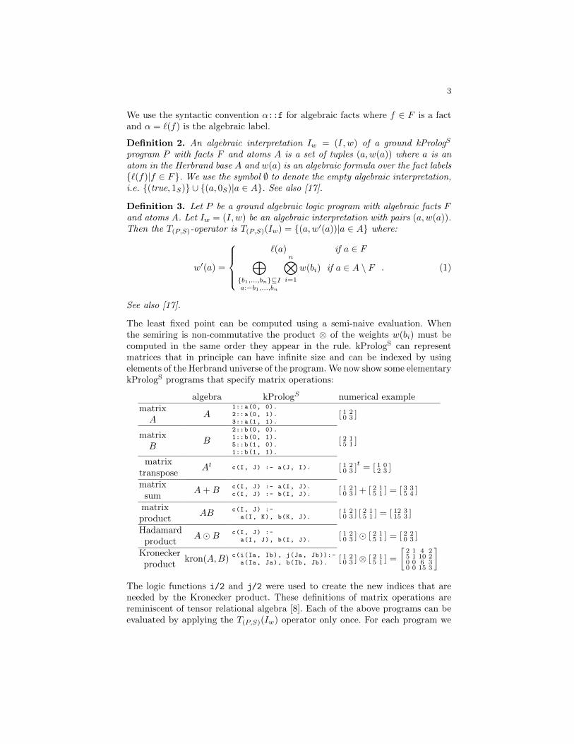
The least fixed point can be computed using a semi-naive evaluation. Whenthe semiring is non-commutative the product ⊗ of the weights w(bi) must becomputed in the same order they appear in the rule. kPrologS can representmatrices that in principle can have infinite size and can be indexed by usingelements of the Herbrand universe of the program. We now show some elementarykPrologS programs that specify matrix operations:

algebra kPrologS numerical examplematrixA

A1::a(0, 0).2::a(0, 1).3::a(1, 1).

[ 1 20 3 ]

matrixB

B

2::b(0, 0).1::b(0, 1).5::b(1, 0).1::b(1, 1).

[ 2 15 1 ]

matrixtranspose

At c(I, J) :- a(J, I). [ 1 20 3 ]

t= [ 1 0

2 3 ]

matrixsum

A+B c(I, J) :- a(I, J).c(I, J) :- b(I, J). [ 1 2

0 3 ] + [ 2 15 1 ] = [ 3 3

5 4 ]

matrixproduct

AB c(I, J) :-a(I, K), b(K, J). [ 1 2

0 3 ] [ 2 15 1 ] = [ 12 3

15 3 ]

Hadamardproduct

A�B c(I, J) :-a(I, J), b(I, J). [ 1 2

0 3 ]� [ 2 15 1 ] = [ 2 2

0 3 ]

Kroneckerproduct

kron(A,B) c(i(Ia, Ib), j(Ja, Jb)):-a(Ia , Ja), b(Ib , Jb). [ 1 2

0 3 ]⊗ [ 2 15 1 ] =

[2 1 4 25 1 10 20 0 6 30 0 15 3

]The logic functions i/2 and j/2 were used to create the new indices that areneeded by the Kronecker product. These definitions of matrix operations arereminiscent of tensor relational algebra [8]. Each of the above programs can beevaluated by applying the T(P,S)(Iw) operator only once. For each program we

4

have a different definition of the C matrix that is represented by the predicatec/2. As a consequence of Equation 1 all the algebraic labels of the c/2 factsare polynomials in the algebraic labels of the a/2 and b/2 facts. We draw ananalogy between the representation of a sparse tensor in coordinate format andthe representation of an algebraic interpretation. A ground fact can be regardeda tuple of indices/domain elements that uniquely identify the cell of a tensor,the algebraic label of the fact represents the value stored in the cell. In kPrologS

for every atom a in the Herbrand base A the negation of a in an interpretationIw can either be expressed with a sparse representation, by excluding it fromthe interpretation (i.e. a 6∈ Iw) or with a dense representation, including it inthe interpretation with algebraic label 0S (i.e. a ∈ Iw and w(a) = 0S).

Definition 4. An algebraic interpretation Iw = (I, w) is the fixed point of theT(P,S)(Iw)-operator if and only if for all a ∈ A, w(a) ≡ w′(a), where w(a) andw′(a) are algebraic formulae for a in Iw and T(P,S)(Iw) respectively. See also[17].

We denote with T i(P,S) the function composition of T(P,S) with itself i times.

Corollary 1 (application of Kleene’s theorem). If S is an ω-continuoussemiring4 the algebraic system of fixed-point equations Iw = T(P,S)(Iw) admits aunique least solution T∞(P,S)(∅) with respect to the partial order v and T∞(P,S)(∅) is

the supremum of the sequence T 1(P,S)(∅), T

2(P,S)(∅), . . . , T

i(P,S)(∅). So T∞(P,S)(∅) can

be approximated by computing successive elements of the sequence. If the semir-ing satisfies the ascending chain property (see [5] ) then T∞(P,S)(∅) = T i(P,S)(∅)for some i ≥ 0 and T∞(P,S)(∅) can be computed exactly [5].

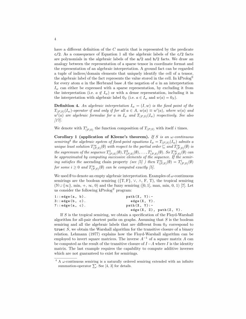
We used ∅ to denote an empty algebraic interpretation. Examples of ω-continuoussemirings are the boolean semiring ({T,F}, ∨, ∧, F, T), the tropical semiring(N ∪ {∞}, min, +, ∞, 0) and the fuzzy semiring ([0, 1], max, min, 0, 1) [7]. Letus consider the following kPrologS program:

1:: edge(a, b).

3:: edge(b, c).

7:: edge(a, c).

path(X, Y):-

edge(X, Y).

path(X, Y):-

edge(X, Z), path(Z, Y).

If S is the tropical semiring, we obtain a specification of the Floyd-Warshallalgorithm for all-pair shortest paths on graphs. Assuming that S is the booleansemiring and all the algebraic labels that are different from 0S correspond totrue∈ S, we obtain the Warshall algorithm for the transitive closure of a binaryrelation. Lehmann (1977) explains how the Floyd-Warshall algorithm can beemployed to invert square matrices. The inverse A−1 of a square matrix A canbe computed as the result of the transitive closure of I−A where I is the identitymatrix. The last example requires the capability to compute additive inverseswhich are not guaranteed to exist for semirings.

4 A ω-continuous semiring is a naturally ordered semiring extended with an infinitesummation-operator

∑. See [4, 3] for details.

5

3 kProlog

kProlog generalizes kPrologS allowing multiple semirings and meta-functions.The coexistence of multiple semirings in the same program requires the decla-ration of the semiring of each algebraic predicate with the directive:

:- declare(<predicate >/<arity >, <semiring >).

We introduce meta-functions and meta-clauses to overcome the limits imposedby the semiring sum and product operations.

Definition 5 (meta-function). A meta-function m: S1 × . . . × Sm → S′ isa function that maps m semiring values xi ∈ Si, i = 1, . . . , k to a value oftype S′, where S1, . . . , Sk and S′ can be distinct semirings. Let a_1,...,a_k bealgebraic atoms, the syntax @m[a_1,...,a_k] expresses that the meta-function@m is applied to the semiring values of the atoms a_1,...,a_k.

Definition 6 (meta-clause). In the kProlog language a meta-clauseh :- b_1,...,b_n is a universally quantified expression where h is an atomand b_1,...,b_n can be either body atoms or meta-functions applied to otheralgebraic atoms. For a given meta-clause, if the head is labeled with the semiringS, also the labels of the body atoms and the return types of the meta-functionsmust be on the semiring S.

Definition 7 (kProlog program). A kProlog program P is a union of kPrologSi

programs and meta-clauses.

The introduction of meta-functions in kProlog allows us to deal with other al-gebraic structures such as rings that require the additive inverse @minus/1 andfields that require the additive inverse and the multiplicative inverse @inv/1.

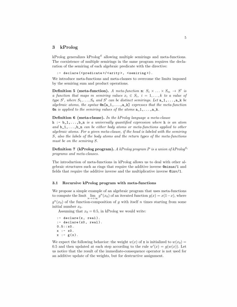
3.1 Recursive kProlog program with meta-functions

We propose a simple example of an algebraic program that uses meta-functionsto compute the limit lim

n→+∞gn(x0) of an iterated function g(x) = x(1−x), where

gn(x0) of the function-composition of g with itself n times starting from someinitial number x0.

Assuming that x0 = 0.5, in kProlog we would write:

:- declare(x, real).

:- declare(x0 , real).

0.5::x0.

x :- x0.

x :- g(x).

We expect the following behavior: the weight w(x) of x is initialized to w(x0) =0.5 and then updated at each step according to the rule w′(x) = g(w(x)). Letus notice that the result of the immediate-consequence operator is not used foran additive update of the weights, but for destructive assignment.

6

We could also consider an additive update rule w′(x) = w(x) + g(w(x)), butthis would not lead to the expected result for an iterated function system.

While iterated function systems require an update with destructive assign-ment, other programs such as the transitive closure of a binary relation (seeabove) or the compilation of ProbLog programs with SDDs require additiveupdates.5

Both additive and destructive updates are allowed in kProlog to increasethe expressivity of the language. We specialize the directive declare/2 intodeclare/3 to make the interpreter aware of the nature (e.g. destructive or ad-ditive) of the update:

:- declare(<predicate >/<arity >, <semiring >, <update -type >).

where update-type can be either additive or destructive. The directivedeclare/3 is only needed for cyclic programs for the predicates whose ground-ings appear in cycles. In case the directive declare/3 was not specified this canbe detected by the system at evaluation time.

To make our program correct we would need to replace :- declare(x, real).

with :- declare(x, real, destructive).

3.2 The Jacobi method

We already showed that kProlog can express linear algebra operations, we nowcombine recursion and meta-functions in an algebraic program that specifies theJacobi method.

The Jacobi method is an iterative algorithm used for solving diagonally dom-inant systems of linear equations Ax = b.

We consider the field of real numbers R (i.e. kPrologR) as semiring togetherwith the meta-functions @minus and @inv that provide the inverse element ofsum and product respectively.

The A matrix must be split according to the Jacobi method:

D = diag(A) d(I, I) :- a(I, I).

R = A−D r(I, J) :- a(I, J), I \= J.

The solution x∗ of Ax = b is computed iteratively by finding the fixed point ofx = D−1(b − Rx). We call E the inverse of D. Since D is diagonal also E is adiagonal matrix:

eii =invert(dii) = 1dii

e(I, I) :- @invert[d(I, I)].

and the iterative step can be rewritten as x = E(b−Rx).Making the summations explicit we can write:

xi = eik

(bk −

∑l

rklxl

)(2)

5 The compilation of ProbLog programs [17] can be expressed in kProlog, provided

7

then we can extrapolate the term∑l

rklxl turning it into the auxk definition:

xi = eik (bk − auxk)

auxk =∑l

rklxl

:- declare(x/1, real , destructive ).:- declare(aux/1, real , destructive ).x(I) :-

e(I, K), @subtraction[b(K), aux(K)].

aux(I) :-r(K, L), x(L).

where @subtraction/2 represents the subtraction between real numbers, x/1and aux/1 are mutually recursive predicates. Because x/1 needs to be initialized(perhaps at random) we also need the clause:

xi = initi x(I) :- init(I).

where init/1 is a unary predicate.This example also shows that kProlog is more expressive than tensor rela-

tional algebra because it supports recursion.

3.3 kProlog TP -operator with meta-functions

The algebraic TP -operator of kProlog is defined on the meta-transformed pro-gram.

Definition 8 (meta-transformed program). A meta-transformed kPrologprogram is a kProlog program in which all the meta-functions are expanded to al-gebraic atoms. For each rule h :- b_1,...,@m[a_1,...,a_k],...,b_n in theprogram P each meta-function @m[a_1,...,a_k] is replaced by a body atom b’

and a meta-clause b’:-@m[a_1,...,a_k] is added to the program P .

Definition 9 (algebraic TP -operator with meta-functions). Let P be meta-transformed kProlog program with facts F and atoms A. Let Iw = (I, w) be analgebraic interpretation with pairs (a,w(a)). Then the TP -operator is TP (Iw) ={(a,w′(a))|a ∈ A} where:

w′(a) =

`(a) if a ∈ F⊕

{b1,...,bn}⊆Ia:−b1,...,bn

n⊗i=1

w(bi)⊕⊕

{b1,...,bk}⊆Ia:−@m[b1,...,bk]

m(w(b1), . . . , w(bk)) if a ∈ A \ F .

(3)

The introduction of meta-functions makes the result of the evaluation of a kPro-log program dependent on the order in which rules and meta-clauses are evalu-ated. For this reason we explain the order adopted by the kProlog language. AkProlog program P is grounded to a program ground(P ) and then partitionedinto a sequence of strata P1, . . . , Pn.

8

An atom in a non-recursive stratum Pi can only depend on the atoms fromthe previous strata

⋃j<i Pj , while a recursive stratum can depend on the atoms

in⋃j≤i Pj .

6 Each partition Pi must be maximal and strongly connected (i.e.each atom in Pi depends on every other atom in Pi). The program evaluationstarts by initializing the weight w(a) of each ground atom a in ground(P ) with0S where S is the semiring of the atom. Then the strata are visited in order andthe weights are updated as follows: if the stratum Pi is non-recursive we applythe algebraic TP -operator only once per atom, while if Pi is recursive we applythe algebraic TP -operator only once for the non-recursive rules and meta-clausesand repeatedly until convergence for the recursive rules and meta-clauses.

When updating the weight w(a) of a recursive atom a at each iteration weinitialize a weight ∆w(a) = 0s. We accumulate on ∆w(a) the result of theapplication of the TP -operator on all the recursive rules with head a. Then thenew weight for a is computed as w(a) = w(a) + ∆w(a) or w(a) = ∆w(a) foradditive and destructive update respectively.7

If Pi is a cyclic stratum then the converge of the algebraic TP -operator mustbe guaranteed by the user that specifies the program. Nevertheless if the Pi is acyclic stratum in which only rules are cyclic all the atoms in Pi are on the samesemiring8 S and so Pi has the same convergence properties of a kPrologS program(see corollary 1 on page 4). Whenever we apply the algebraic TP -operator weuse the Jacobi evaluation, so that the program is not affected by the order inwhich rules and meta-clauses are evaluated. This program evaluation procedureis an adaptation the work of Whaley et al. (2005) on Datalog and binary decisiondiagrams.

4 kPrologS[x]

kPrologS[x] labels facts and rule heads with polynomials over the semiring S.kPrologS[x] is a particular case of kPrologS because polynomials over semiringsare semirings in which addition and multiplication are defined as usual.

Definition 10 (Multivariate polynomials over commutative semirings).A multivariate polynomial P ∈ S[x] can be expressed as:

P(x) =

n⊕i=1

cixei =

n⊕i=1

ci ⊗⊗t∈Ti

xeitt (4)

that the SDD semiring is used. The update of the algebraic weights must be additive,each update adds new proves for the ground atoms until convergence.

6 We say that an atom a directly depends on an atom b if a is the head of a rule or ameta-clause and b is a body literal or an argument of a meta-function in the metaclause. We say that an atom a depends on an atom b either if a directly dependson b or there is an atom c such that a directly depends on c and c depends on b.

7 The update type is specified in the language by using the declare/3 directive.8 atoms of distinct semirings cannot be mutually dependent without using meta-

clauses

9

where ci ∈ S are the coefficients of the ith monomial and x, e are vectors ofvariables and exponents respectively. The vector x is indexed by ground termst ∈ T .

4.1 Polynomials for feature extraction

We shall use polynomials to represent kernel features such as the ones computedby the Weisfeiler-Lehman and propagation kernels. We define an inner-productbetween multivariate polynomials of R[x], with a finite number of monomials as:

〈P(x),Q(x)〉 =∑

(p,e)∈P

∑(q,e)∈Q

pq. (5)

For each monomial (uniquely identified by the vector of exponents e) that ap-pears in both the polynomials P and Q, Equation 5 computes the product be-tween their coefficients p and q respectively. These products are then summedtogether to obtain the value of the inner-product. The inner-product between twoalgebraic atoms P(x)::a and Q(x)::b can be computed using the meta-function@dot/2. Another meta-function, that is useful for kernel design, is @rbf/3. Themeta-function @rbf/3 takes as input an atom labeled with a non-negative realvalue γ and two atoms labeled with the polynomials P and Q and computes therbf kernel exp{−γ‖P −Q‖2}.9

4.2 The @id meta-function

The @id/1 meta-function @id: S → S is injective and transforms a polynomialP(x) to a new term t and returns the polynomial @id[P(x)] = 1.0 · x(t). Thisfunction can be used to compress a multivariate polynomial to a new polynomialin a single variable. We use the @id meta-function for polynomial compressionas Shervashidze et al. ( 2011) use the function f to compress multisets of labels.

Indeed we can represent a multiset µ of labels (we use Prolog ground termsto represent labels) as a polynomial:

Pµ(x) =∑t∈µ

]t · x(t) (6)

where ] counts the number of occurrences of the label (identified by the groundterm t) in the multiset µ.Weisfeiler-Lehman algorithm: A colored graph G is a triple (V,E, `) whereV is a set of vertices, E ⊆ V × V is the set of the edges and ` : V → Σ is afunction that maps vertices to a color alphabet Σ. For example we can specifyvertex labels and edge connectivity of a graph graph_a in kProlog as follows:

9 The squared distance in the rbf kernel can be expressed by using the dot product,i.e. ‖P −Q‖2 = 〈P,P〉+ 〈Q,Q〉 − 2〈P,Q〉

10

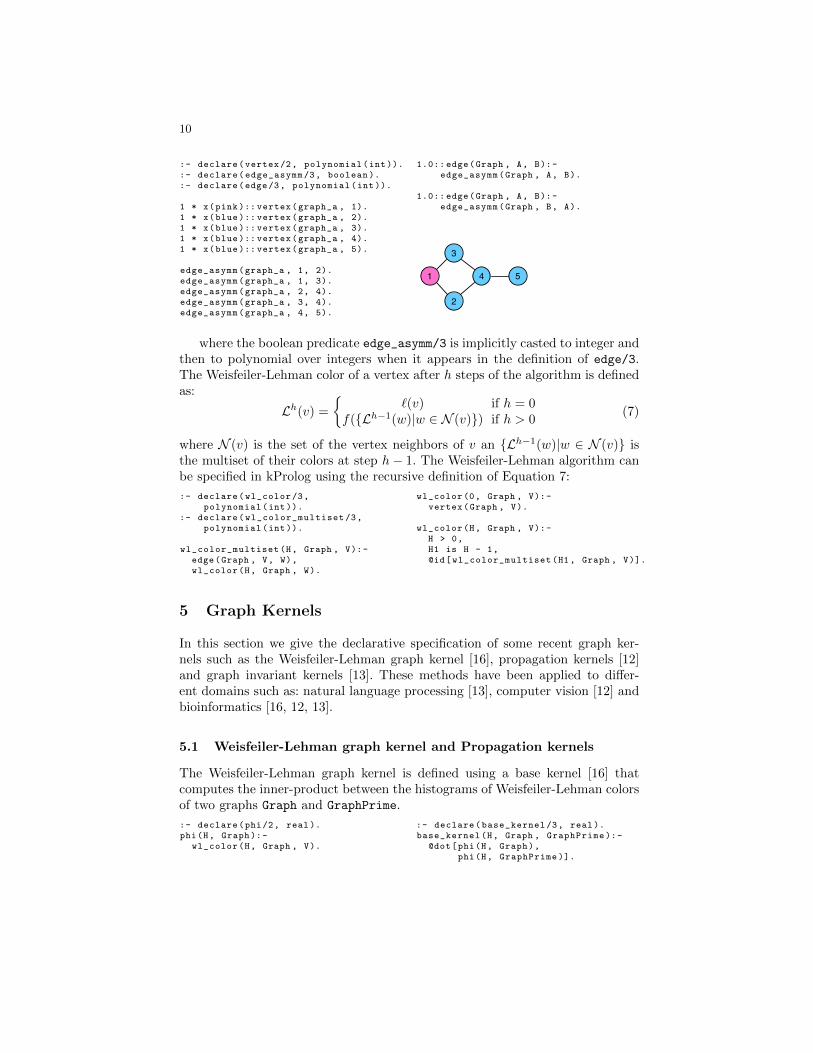
:- declare(vertex/2, polynomial(int)).:- declare(edge_asymm /3, boolean ).:- declare(edge/3, polynomial(int)).

1 * x(pink ):: vertex(graph_a , 1).1 * x(blue ):: vertex(graph_a , 2).1 * x(blue ):: vertex(graph_a , 3).1 * x(blue ):: vertex(graph_a , 4).1 * x(blue ):: vertex(graph_a , 5).

edge_asymm(graph_a , 1, 2).edge_asymm(graph_a , 1, 3).edge_asymm(graph_a , 2, 4).edge_asymm(graph_a , 3, 4).edge_asymm(graph_a , 4, 5).

1.0:: edge(Graph , A, B):-edge_asymm(Graph , A, B).

1.0:: edge(Graph , A, B):-edge_asymm(Graph , B, A).

2

4 5

3

1

where the boolean predicate edge_asymm/3 is implicitly casted to integer andthen to polynomial over integers when it appears in the definition of edge/3.The Weisfeiler-Lehman color of a vertex after h steps of the algorithm is definedas:

Lh(v) =

{`(v) if h = 0

f({Lh−1(w)|w ∈ N (v)}) if h > 0(7)

where N (v) is the set of the vertex neighbors of v an {Lh−1(w)|w ∈ N (v)} isthe multiset of their colors at step h− 1. The Weisfeiler-Lehman algorithm canbe specified in kProlog using the recursive definition of Equation 7:

:- declare(wl_color/3,polynomial(int)).

:- declare(wl_color_multiset /3,polynomial(int)).

wl_color_multiset(H, Graph , V):-edge(Graph , V, W),wl_color(H, Graph , W).

wl_color(0, Graph , V):-vertex(Graph , V).

wl_color(H, Graph , V):-H > 0,H1 is H - 1,@id[wl_color_multiset(H1 , Graph , V)].

5 Graph Kernels

In this section we give the declarative specification of some recent graph ker-nels such as the Weisfeiler-Lehman graph kernel [16], propagation kernels [12]and graph invariant kernels [13]. These methods have been applied to differ-ent domains such as: natural language processing [13], computer vision [12] andbioinformatics [16, 12, 13].

5.1 Weisfeiler-Lehman graph kernel and Propagation kernels

The Weisfeiler-Lehman graph kernel is defined using a base kernel [16] thatcomputes the inner-product between the histograms of Weisfeiler-Lehman colorsof two graphs Graph and GraphPrime.

:- declare(phi/2, real).phi(H, Graph):-

wl_color(H, Graph , V).

:- declare(base_kernel /3, real).base_kernel(H, Graph , GraphPrime ):-

@dot[phi(H, Graph),phi(H, GraphPrime )].

11

The Weisfeiler-Lehman graph kernel [16] with H iterations is the sum of basekernels computed for consecutive Weisfeiler-Lehman labeling steps 1, . . . ,H onthe graphs Graph and GraphPrime:

:- declare(kernel_wl/3, real).kernel_wl(0, Graph , GraphPrime ):-

base_kernel (0, Graph , GraphPrime ).

kernel_wl(H, Graph , GraphPrime ):-H > 0, H1 is H - 1,kernel_wl(H1, Graph , GraphPrime ).

kernel_wl(H, Graph , GraphPrime ):-H > 0,base_kernel(H, Graph , GraphPrime ).

.

Propagation kernels [12] are a generalization of the Weisfeiler-Lehman graph ker-nel, that can adopt different label propagation schemas. Neumann et al. (2012)implements propagation kernels using locality sensitive hashing. The kPrologspecification is identical to the one the Weisfeiler-Lehman except that the @id

meta-function is to be replaced with a meta-function that does locality sensitivehashing.

5.2 Graph invariant kernels

Graph Invariant Kernels (giks, pronounce “geeks”) are a recent framework forgraph kernels with continuous attributes [13].

giks compute a similarity measure between graphs G and G′ matching themat vertex level according to the formula:

k(G,G′) =∑

v∈V (G)

∑v′∈V (G′)

w(v, v′)kattr(v, v′) (8)

where w(v, v′) is the structural weight matrix and kattr(v, v′) is a kernel on thecontinuous attributes of the graphs. We use R-neighborhood subgraphs, so thekProlog specification is parametrized by the variable R.

:- declare(gik_radius /3, real).gik_radius(R, Graph , GraphPrime ):-

w_matrix(R, Graph , V, GraphPrime , VPrime),k_attr(Graph , V, GraphPrime , VPrime ).

where gik_radius/3, w_matrix/5 and k_attr/4 are algebraic predicates onthe real numbers semiring, which is represented with floats for implementationpurposes. Assuming that we want to use the rbf with γ = 0.5 kernel on thevertex attributes we can write:

:- declare(rbf_gamma_const /0, real).:- declare(k_attr/4, real).0.5:: rbf_gamma_const.k_attr(Graph , V, GraphPrime , VPrime):-

@rbf[rbf_gamma_const , attr(Graph , V), attr(GraphPrime , VPrime )].

where attr/2 is an algebraic predicate that associates to the vertex V of a Graph

a polynomial label. To associate to vertex v_1 of graph_a the 4-dimensionalfeature [1, 0, 0.5, 1.3] we would write:

:- declare(attr/2, polynomial(real )).1.0 * x(1) + 0.5 * x(3) + 1.3 * x(4):: attr(graph_a , v_1).

12

while the meta-function @rbf/3 takes as input an atom rbf_gamma_const la-beled with the γ constant and the atoms relative to the vertex attributes.

The structural weight matrix w(v, v′) is defined as:

w(v, v′) =∑

g∈R−1(G)

∑g′∈R−1(G′)

kinv(v, v′)δm(g, g′)

|Vg||Vg′ |1{v ∈ Vg ∧ v′ ∈ Vg′}. (9)

The weight w(v, v′) measures the structural similarity between vertices and isdefined combining anR-decomposition relation, a function δm(g, g′) and a kernelon vertex invariants kinv [13]. In our case the R-decomposition generates R-neighborhood subgraphs (the same used in the experiments of Orsini et al. (2015)).

There are multiple ways to instantiate giks, we choose the version calledlwlv, because as shown with the experiments by Orsini et al. ( 2015), canachieve very good accuracies most of the times.

lwlv uses R-neighborhood subgraphs R-decomposition relation, computesthe kernel on vertex invariants kinv(v, v′) at the pattern level (local gik) anduses δm(g, g′) to match subgraphs that have the same number of nodes.

In kProlog we would write:

:- declare(w_matrix/5, real).w_matrix(R, Graph , V, GraphPrime , VPrime):-

vertex_in_ball(Graph , R, BallRoot , V),vertex_in_ball(GraphPrime , R, BallRootPrime , VPrime),delta_match(R, Graph , BallRoot , GraphPrime , BallRootPrime),@inv[ball_size(R, Graph , BallRoot)],@inv[ball_size(R, GraphPrime , BallRootPrime )],k_inv(Graph , BallRoot , V, GraphPrime , BallRootPrime , VPrime ).

where:a) vertex_in_ball(R, Graph, BallRoot, V) is a boolean predicate whichis true if V is a vertex of Graph inside a R-neighborhood subgraph rooted inBallRoot. vertex_in_ball/4 encodes both the term 1{v ∈ Vg ∧ v′ ∈ Vg′} andthe pattern generation of the decomposition relation g ∈ R−1(G).

:- declare(vertex_in_ball /4, bool).vertex_in_ball (0, Graph , Root , Root):-

vertex(Graph , Root).

vertex_in_ball(R, Graph , Root , V):-R > 0, R1 is R - 1,vertex_in_ball(R1 , Graph , Root , V).

vertex_in_ball(R, Graph , Root , V):-R > 0, R1 is R - 1,edge(Graph , Root , W),vertex_in_ball(R1 , Graph , W, V).

b) delta_match(R, Graph, BallRoot, GraphPrime, BallRootPrime)

matches subgraphs with the same number of vertices

:- declare(delta_match /5, real).:- declare(v_id/3, polynomial(real )).:- declare(ball_size/3, int).

delta_match(R, Graph , BallRoot , GraphPrime , BallRootPrime ):-@eq[v_id(R, Graph , BallRoot), v_id(R, GraphPrime , BallRootPrime )].

v_id(R, Graph , BallRoot):- @id[ball_size(R, Graph , BallRoot )].

ball_size(R, Graph , BallRoot):- vertex_in_ball(R, Graph , BallRoot , V).

13

c) @inv[ball_size(Radius, Graph, BallRoot)] corresponds to the normal-ization term 1/|Vg|. @inv is the meta-function that computes the multiplicativeinverse and ball_size(Radius, Graph, BallRoot) is a the float predicate thatcounts the number of vertices in a Radius-neighborhood rooted in BallRoot.d) k_inv(R, Graph, BallRoot, V, GraphPrime, BallRootPrime, VPrime)

computes kinv using H_WL iterations of the Weisfeiler-Lehman algorithm to obtainvertex features phi_wl(R, H_WL, Graph, BallRoot, V) from the R-neighborhoodsubgraphs.

:- declare(k_inv/7, real).:- declare(phi_wl/5, polynomial(real )).wl_iterations (3). % constant

k_inv(R, Graph , BallRoot , V, GraphPrime , BallRootPrime , VPrime):-wl_iterations(H_WL),@dot[phi_wl(R, H_WL , Graph , BallRoot , V),

phi_wl(R, H_WL , GraphPrime , BallRootPrime , VPrime )].

phi_wl(R, 0, Graph , BallRoot , V):-wl_color(R, Graph , BallRoot , 0, V).

phi_wl(R, H, Graph , BallRoot , V):-H > 0, wl_color(R, Graph , BallRoot , H, V).

phi_wl(R, H, Graph , BallRoot , V):-H > 0, H1 is H-1,phi_wl(R, H1, Graph , BallRoot , V).

where wl_color/5 is defined as wl_color/3, but has two additional argumentsR and BallRoot that are needed to restrict the graph connectivity to the R-neighborhood subgraph rooted in vertex BallRoot.

6 Conclusions

We proposed kProlog, a simple algebraic extension of Prolog that can be used forkernel programming. Polynomials and meta-functions allow to elegantly specifyin kProlog many recent kernels (e.g the Weisfeiler-Lehman Graph kernel, prop-agation kernels and giks). kProlog rules are used for kernel programming, butalso to incorporate background knowledge and enrich the input data representa-tion with user specified relations. kProlog is a language that provides a uniformrepresentation for relational data, background knowledge and kernel design. Inour future work we will exploit these three characteristics of kProlog to learnfeature spaces with inductive logic programming.

Bibliography

[1] L De Raedt, A Kimmig, and H Toivonen. Problog: A probabilistic prolog and itsapplication in link discovery. In IJCAI, 2007.

[2] J Eisner and N W Filardo. Dyna: Extending datalog for modern ai. In DatalogReloaded. Springer, 2011.

[3] Javier Esparza and Michael Luttenberger. Solving fixed-point equations by deriva-tion tree analysis. In Algebra and Coalgebra in Computer Science. Springer, 2011.

[4] Javier Esparza, Stefan Kiefer, and Michael Luttenberger. An extension of newtonsmethod to ω-continuous semirings. In Developments in Language Theory. Springer,2007.

[5] J Esparza, M Luttenberger, and M Schlund. Fpsolve: A generic solver for fixpointequations over semirings. In Implementation and Application of Automata. Springer,2014.

[6] P Frasconi, F Costa, L De Raedt, and K De Grave. klog: A language for logicaland relational learning with kernels. Artificial Intelligence, 2014.

[7] Todd J Green, Grigoris Karvounarakis, and Val Tannen. Provenance semirings. InProceedings of the 26th ACM SIGMOD-SIGACT-SIGART symposium on Principlesof database systems. ACM, 2007.

[8] M Kim and K S Candan. Approximate tensor decomposition within a tensor-relational algebraic framework. In Proceedings of the 20th ACM international con-ference on Information and knowledge management. ACM, 2011.

[9] A Kimmig, G Van den Broeck, and L De Raedt. An algebraic prolog for reasoningabout possible worlds. In 25th AAAI Conference on Artificial Intelligence, 2011.

[10] N Landwehr, A Passerini, L De Raedt, and P Frasconi. kfoil: Learning simplerelational kernels. In AAAI, 2006.

[11] Daniel J Lehmann. Algebraic structures for transitive closure. Theoretical Com-puter Science, 1977.

[12] M Neumann, N Patricia, R Garnett, and K Kersting. Efficient graph kernelsby randomization. In Machine Learning and Knowledge Discovery in Databases.Springer, 2012.

[13] F Orsini, P Frasconi, and L De Raedt. Graph invariant kernels. In Proceedings ofthe 24th IJCAI, 2015.

[14] M Richardson and P Domingos. Markov logic networks. Machine learning, 2006.[15] T Sato and Y Kameya. Prism: a language for symbolic-statistical modeling. In

IJCAI, 1997.[16] N Shervashidze, P Schweitzer, E J Van Leeuwen, K Mehlhorn, and K M Borg-

wardt. Weisfeiler-lehman graph kernels. The Journal of Machine Learning Research,2011.

[17] J Vlasselaer, G Van den Broeck, A Kimmig, W Meert, and L De Raedt. Anytimeinference in probabilistic logic programs with tp-compilation. In Proceedings of the24th IJCAI, 2015.

[18] J Whaley, D Avots, M Carbin, and M S Lam. Using datalog with binary decisiondiagrams for program analysis. In Programming Languages and Systems. Springer,2005.