Embed Size (px)
Citation preview

This draft was prepared using the LaTeX style file belonging to the Journal of Fluid Mechanics 1
Koopman mode expansions between simpleinvariant solutions
Jacob Page† & Rich R. Kerswell‡DAMTP, Center for Mathematical Sciences, University of Cambridge, Cambridge, CB3 0WA,
UK
(Received xx; revised xx; accepted xx)
A Koopman decomposition is a powerful method of analysis for fluid flows leading toan apparently linear description of nonlinear dynamics in which the flow is expressed as asuperposition of fixed spatial structures with exponential time dependence. Attemptinga Koopman decomposition is simple in practice due to a connection with Dynamic ModeDecomposition (DMD). However, there are non-trivial requirements for the Koopmandecomposition and DMD to overlap which mean it is often difficult to establish whetherthe latter is truly approximating the former. Here, we focus on nonlinear systemscontaining multiple simple invariant solutions where it is unclear how to construct aconsistent Koopman decomposition, or how DMD might be applied to locate thesesolutions. First, we derive a Koopman decomposition for a heteroclinic connection ina Stuart-Landau equation revealing two possible expansions. The expansions are centredabout the two fixed points of the equation and extend beyond their linear subspaces beforebreaking down at a crossover point in state space. Well-designed DMD can extract thetwo expansions provided that the time window does not contain this crossover point.We then apply DMD to the Navier-Stokes equations near to a heteroclinic connection inlow-Reynolds number (Re = O(100)) plane Couette flow where there are multiple simpleinvariant solutions beyond the constant shear basic state. This reveals as many differentKoopman decompositions as simple invariant solutions present and once more indicatesthe existence of crossover points between the expansions in state space. Again, DMDcan extract these expansions only if it does not include a crossover point. Our resultssuggest that in a dynamical system possessing multiple simple invariant solutions, thereare generically places in phase space – plausibly hypersurfaces delineating the boundaryof a local Koopman expansion – across which the dynamics cannot be represented by aconvergent Koopman expansion.
Key words:
1. Introduction
In the past few decades the discovery of non-trivial exact solutions of the Navier-Stokesequations has given rise to a dynamical systems view of turbulent flow (Kerswell 2005;Eckhardt et al. 2007; Kawahara et al. 2012). In this perspective, a turbulent orbit wandersin phase space between these so-called exact coherent structures or simple invariantsolutions (e.g. equilibria, travelling waves, periodic orbits), pulled in along their stable

2 J. Page & R. R. Kerswell
manifolds and thrown out along their unstable manifolds (Gibson et al. 2008, 2009).Individually, exact coherent structures can offer a useful perspective on the fully turbulentdynamics: their averaged properties often share qualitative similarities to statistics of theturbulence while their simple time dependence makes the underlying physical mechanismsfar simpler to extract and analyse (e.g. Waleffe 1997; Kawahara & Kida 2001; Wang et al.2007; Hall & Sherwin 2010). Since the discovery of the first pair of non-trivial equilibriain plane Couette flow by Nagata (1990), exact coherent structures have been found ina wide range of flow geometries (Waleffe 1997, 2001; Faisst & Eckhardt 2003; Wedin &Kerswell 2004; Gibson et al. 2008, 2009; Uhlmann et al. 2010), in spatially extended flows(Schneider et al. 2010; Avila et al. 2013; Chantry et al. 2014; Zammert & Eckhardt 2014;Gibson & Brand 2014; Brand & Gibson 2014) and in stratified fluids (Olvera & Kerswell2017; Deguchi 2017; Lucas et al. 2017).
A crucial step in attempting to converge exact solutions of the Navier-Stokes equationsis the generation of an initial guess for the structure of interest, which is then fed into aNewton-Raphson algorithm. For an equilibrium the guess takes the the form of a velocitysnapshot; for periodic orbits the snapshot must be supplemented with a guess for theperiod. Currently, methods for generating guesses include (i) edge tracking (Schneideret al. 2007), (ii) using snapshots of turbulence (equilibria only, Gibson et al. 2009),(iii) using reduced representations of known solutions (Ahmed & Sharma 2017), (iv)branch continuation of known solutions (Nagata 1990; Waleffe 2001; Faisst & Eckhardt2003; Wedin & Kerswell 2004) or (v) a recurrent flow analysis (Kawahara & Kida 2001;Viswanath 2007; Cvitanovic & Gibson 2010; Chandler & Kerswell 2013). Each of theseapproaches has weaknesses, for example continuation cannot find unconnected solutionswhile recurrent flow analysis requires the turbulent flow to shadow a periodic orbit forat least one cycle – increasingly improbable as the Reynolds number is increased.
The recent emergence of Dynamic Mode Decomposition (DMD) suggests an alternativeapproach to finding exact coherent structures in nonlinear simulation data. DMD wasoriginally invented by Schmid (2010) as a post-processing technique for simulation orexperimental data, with many variants on the algorithm developed since (e.g. Jovanovicet al. 2014; Williams et al. 2015). DMD finds a linear operator that best maps (in aleast squares sense) between equispaced snapshots of the flow. As a result of which theflow can then be expressed as a superposition of dynamic “modes” (eigenvectors of theDMD operator) with an exponential dependence on time. An attractive feature of themethod is that it can identify frequencies of oscillation in the flow which correspond toperiods far longer than the time window over which observations are recorded. Beyondfluid mechanics, DMD has already been applied in areas as diverse as video processing(Kutz et al. 2016b) and neuroscience (Brunton et al. 2016a).
Connecting the output of DMD with exact coherent structures rests on its connectionto the Koopman operator which is a linear infinite dimensional operator that evolvesfunctionals (or observables) of the velocity field forward in time (Koopman 1931; Mezic2005, 2013). Koopman operator theory asserts that the nonlinear evolution of observablesof the state, u, can be expressed as a sum of fixed spatial structures (Koopman modes)with an exponential time dependence. This is accomplished through a projection ontoeigenfunctions of the Koopman operator, which are special scalar observables of thesystem which evolve like exp(λt), where λ is the associated Koopman eigenvalue. Mezic(2005) showed that such a representation can be constructed for dynamical systems withan invariant measure, in which Koopman eigenfunctions are (proportional to) “harmonicaverages” at certain frequencies (e.g. Mezic & Banaszuk 2004) and the eigenvalues {λi}are all purely imaginary. In addition to these discrete eigenvalues, the Koopman operatorin chaotic systems typically also has a continuous spectrum (e.g. see Arbabi & Mezic 2017,

Koopman expansions 3
for a nice example showing the increasing dominance of this component in the overalldynamics with increasing Reynolds number).
Individual exact coherent structures have a particularly simple interpretation in termsof Koopman eigenfunctions. For example, Mezic (2017) constructed Koopman decompo-sitions for nonlinear systems with a single attracting simple invariant set. The Koopmaneigenvalues associated with a periodic orbit, for example, are purely imaginary repeatedharmonics of the fundamental frequency. In addition, there is an infinite lattice ofdecaying eigenvalues, which can be obtained from the linear Floquet multipliers (seealso Bagheri 2013, for an explicit demonstration of this). This raises an interesting issuein shear flows which support long-time turbulent dynamics and also feature a myriad ofexact coherent structures (e.g. minimal Couette flow Hamilton et al. 1995; Cvitanovic &Gibson 2010): How are the Koopman eigenfunctions associated with local dynamics inthe vicinity of an exact coherent structure connected to the eigenfunctions ‘associatedwith’ the invariant measure, or long-time dynamics, of a turbulent flow?
Koopman eigenfunctions have been obtained analytically in some simple nonlinearordinary differential equations (e.g. Bagheri 2013; Brunton et al. 2016b; Rowley &Dawson 2017) and recently for Burgers’ equation which can be linearized by the Cole-Hopf transformation (Page & Kerswell 2018). However, it is unlikely that closed-formexpressions for Koopman eigenfunctions of the Navier-Stokes equations can be writtendown, and most DMD-based studies focus on extracting the Koopman modes (Rowleyet al. 2009; Bagheri 2013; Tu et al. 2014) which under certain requirements overlap withdynamic modes (Tu et al. 2014; Williams et al. 2015). There are two requirements forDMD and Koopman to coincide: (i) that sufficient data is available and (ii) that theKoopman eigenfunctions can be expressed as a linear combination of the functionals ofthe state which serve as the inputs to the DMD algorithm (Williams et al. 2015). Thesecond point is difficult to enforce in practice and various strategies have been proposed toensure the input function space is sufficiently ‘rich’ (e.g. ‘Kernel’ based methods, see Kutzet al. 2016a). Furthermore, even if DMD can accurately extract Koopman eigenfunctions,there is no guarantee that these then form a basis for the state variable itself (e.g Bruntonet al. 2016b; Page & Kerswell 2018). Alongside DMD, a variety of other methods havebeen proposed to extract Koopman eigenfunctions and modes from fluid flows that maycircumvent some of these issues. For example, Arbabi & Mezic (2017) applied harmonicaveraging (Mezic & Banaszuk 2004) to highly turbulent lid-driven cavity flow to identifyKoopman eigenfunctions and modes associated with its attracting limit cycle, whileSharma et al. (2016) demonstrated a connection between Koopman modes and modesof the resolvent operator. There have also been some interesting attempts to use neuralnetworks to identify the nonlinear mappings that ‘linearize’ the dynamics (Lusch et al.2018) - the Koopman eigefunctions - though these have so far been restricted to low-dimensional examples.
Our focus in this study is on the utility of DMD as a tool to identify exact coherentstructures and their stable and unstable manifolds. As well as the possible intriguingconnections between Koopman eigenfunctions associated with unstable simple invariantsets and those associated with long-time averages, there are further known issues relatedto both DMD and Koopman analysis in systems with more than one simple invariantsolution. For example, Brunton et al. (2016b) have demonstrated that it is not possible toform a Koopman invariant subspace that contains the state variable itself in a nonlinearsystem with more than one fixed point, indicating that there is not a single uniformlyvalid Koopman expansion. This fact may have implications for DMD and its abilityto find Koopman eigenvalues, and there is reason to believe that this issue has beenencountered in past studies. Bagheri (2013) performed a multiple-scales analysis to

4 J. Page & R. R. Kerswell
analytically construct a Koopman decomposition for flow past a cylinder just beyondthe critical Reynolds number. The expansion describes the transient collapse onto theoscillatory limit cycle (vortex shedding). However, Bagheri (2013) could only match hisanalytical result to the output of DMD provided that the DMD observation window didnot stretch too far back into the region of “transient amplification”. Eaves et al. (2016)found similar results when performing DMD on a flow trajectory approaching and thenreceding from the fixed point edge state in small-box plane Couette flow.
In this paper we seek to bring some clarity to these issues by considering a pair ofexamples: a model ODE system with two fixed points and the Navier-Stokes equationswith multiple solutions. We demonstrate that each simple invariant solution has anassociated Koopman expansion for the state variable which extends beyond the respectivelinear subspace but which breaks down at a point in state space. These crossover pointsimpact the ability of DMD to extract a Koopman decomposition from the data – aDMD calculation with an observation window including a crossover point will fail.The structure of the remainder of this paper is as follows. In §2 we briefly reviewthe basics of Koopman mode decompositions before describing a new approach fortheir computation given a solution to a nonlinear equation. The results are appliedto the Stuart-Landau equation and compared to DMD. In §3 we extend these ideasto the Navier-Stokes equations, using DMD to find Koopman mode decompositionsalong heteroclinic connections between simple invariant solutions in low Reynolds planeCouette flow. Finally, concluding remarks are provided in §4.
2. Koopman mode decompositions of a Stuart-Landau equation
2.1. The Koopman operator
We consider nonlinear dynamical systems of the form
∂tu = F(u), (2.1)
with the time-forward map f t(u) = u +∫ t0
F(u)dt′. The Koopman operator, K t, is aninfinite-dimensional linear operator that propagates functionals ψ of the state vector - or“observables” - forward in time (Koopman 1931; Mezic 2005) along a trajectory of (2.1),
K tψ(u) := ψ(f t(u)). (2.2)
The eigenfunctions of this linear, infinite-dimensional operator are special observableswith exponential time dependence
K tϕλ(u) = ϕλ(u)eλt. (2.3)
It then follows that Koopman eigenfunctions can be computed by the relation
dtϕλ(u) = F(u) ·∇uϕλ(u) = λϕλ(u). (2.4)
The default assumption is then that the Koopman eigenfunctions can be used to expanda vector of observables,
ψ(u) =∑n
ϕλn(u)ψn, (2.5)
where the coefficients ψn are called Koopman modes (Rowley et al. 2009). A commonchoice is to consider a spatially-varying functional so that the vector ψ(u) is just thatfunctional evaluated over a discretization of space. In this case, the nonlinear evolutionof ψ(u) is expressed as a superposition of fixed spatial structures (the Koopman modes)with an exponential time-dependence (through the Koopman eigenfunctions), giving the

Koopman expansions 5
appearance of linearity. Representations like (2.5) as applied to turbulent flows typicallyfeature an additional term associated with a continuous spectrum of eigenvalues (Mezic2005, 2013). In these applications the Koopman eigenvalues are all purely imaginary,and the discrete terms appearing in (2.5) consist of a long-time average (eigenvalueλ0 = 0) and ‘harmonic averages’ at discrete frequencies λ = iω. However, individual exactcoherent structures have their own associated Koopman eigenfunctions, and our interestis in building local decompositions around these solutions (which may be embedded in aturbulent attractor). It is at present unclear how such an expansion might be constructedfor a turbulent trajectory that visits multiple simple invariant solutions. For example, ina system with multiple equilibria, one would expect each fixed point to correspond toa neutral eigenfunction of the Koopman operator leading to a degeneracy of the λ = 0eigenvalue.
2.2. Stuart-Landau equation
For a simple example with multiple equilibria, we first revisit the problem consideredin Bagheri (2013) – an analytical derivation of the Koopman decomposition for solutionsto a Stuart-Landau equation,
dA
dt= a0A− a1A|A|2. (2.6)
Following Bagheri (2013), we write the complex amplitude in polar coordinate, A(t) =r(t)exp[iθ(t)]. In our analysis we neglect the dependence on θ(t) by assuming a0 := µ ∈ Rand without loss of generality a1 := 1 to focus solely on the evolution of amplitudevariable r(t). The angular dependence is straightforward to incorporate and its inclusiononly complicates the presentation. The evolution equation for r(t) is
dr
dt= µr − r3 (2.7)
which has a pitchfork bifurcation at µ = 0; for µ > 0 there are attractors at r = ±√µand a repellor at r = 0. Similar to Bagheri (2013), we consider trajectories for whichr(t = 0) > 0 and r(t→∞)→ √µ and seek a Koopman representation for an observableψ(r). However, rather than inverse-engineering the Koopman eigenfunctions, eigenvaluesand modes from a Fourier expansion around the limit cycle (appendix A in Bagheri(2013)), we identify them directly from the relationship (2.4). Since this holds universallyacross the dynamics and not just close to any simple invariant solution, we can constructKoopman representations for the full lifespan of the solution trajectory. Interestingly,two different non-overlapping representations emerge, one centred around the repellor(r = 0) and the other around the attractor (r =
√µ), which meet at a “cross-over” point
where both fail simultaneously to converge. Our analysis is complementary to the studyby Gaspard et al. (1995), who examined the evolution of probability densities under thedynamics described by (2.7).
2.3. Koopman mode decompositions
Assuming µ > 0, equation (2.7) can be rescaled with R := r/√µ and T := µt to
dR
dT= R−R3 =: f(R) (2.8)
which has solution
R(T ;R0) =1√
1 + b(R0)e−2T, (2.9)

6 J. Page & R. R. Kerswell
where b(R0) := (1 − R20)/R2
0 so R(0;R0) = R0. Our aim is to write the evolution ofan observable, ψ(R), as an expansion in eigenfunctions of the Koopman operator. Forthis one dimensional example, equation (2.4) for the Koopman eigenfunctions becomessimply
f(R)dϕλdR
= λϕλ (2.10)
which has solution
ϕλ(R) =
(R2
1−R2
)λ/2= ϕλ(R0)eλT (2.11)
where formally λ can be any complex number. The unstable eigenfunctions ϕλ>0 aresingular at the attracting fixed point R = 1 and the temporally-decaying ϕλ<0 aresingular at the repeller R = 0. In order to be able to build expansions around the twoequilibria R = 0 and R = 1, the eigenfunctions presumably need to be analytic in theneighbourhood of one of these equilibria which means λ ∈ R at least.
There are another set of (weak) eigensolutions in this problem that solve∫f(R)
dϕλdR
w(R)dR = λ
∫ϕλ(R)w(R)dR, (2.12)
where w(R) is a smooth weight function. The eigensolutions are
ϕλn(R) = δ(n)(
1−R2
R2
), λn = 2(n+ 1) n ∈ N ∪ {0}, (2.13)
and
ϕλn(R) = δ(n)(
R2
1−R2
), λn = −2(n+ 1) n ∈ N ∪ {0}, (2.14)
where δ(n) is the nth derivative of the delta distribution. These eigenmeasures consist ofone family that exhibits exponential growth (2.13) at the stable fixed point(s) and anotherwhich is decaying (2.14) at the repellor. They were originally identified by Gaspard et al.(1995), and are important if the goal is to compute the time evolution of densities, sinceKoopman eigenfunctions are bi-orthogonal to eigenfunctions of the Perron-Frobeniusoperator (Gaspard 1998). In that problem, solving the initial value problem for thedensity is challenging since the inclusion of (2.13) and (2.14) alongside (2.11) introducesa degeneracy. However, these eigensolutions are not required to express the evolution ofobservables we are interested in (namely the state itself) and we can safely ignore them.
In the absence of the eigenmeasures discussed above, there is a single one-parameterfamily of Koopman eigenfunctions (2.11) and a continuous spectrum of eigenvalues. AKoopman representation for a general observable would then be
ψ(R) =
∫ ∞−∞
aψ(−λ)ϕ−λ(R)dλ,
=
∫ ∞−∞
aψ(−λ)ϕ−λ(R0)e−λTdλ (2.15)
where aψ(−λ) is the Koopman mode density for the observable ψ corresponding to theKoopman eigenvalue −λ. Writing the integrand in terms of −λ highlights the fact thatthe expression (2.15) is a bilateral Laplace transform with λ playing the role of thetime-like variable and T the transform variable. Setting ψ = R, which is often the first

Koopman expansions 7
observable of interest, we write
R(T ) =
∫ ∞−∞
a(−λ)ϕ−λ(R0)e−λTdλ. (2.16)
and then the inverse Laplace transform inversion in the complex-T plane
a(−λ)ϕ−λ(R0) =1
2πi
∫ γ+i∞
γ−i∞R(T )eλTdT =
1
2πi
∫ γ+i∞
γ−i∞
eλT√1 + b(R0)e−2T
dT (2.17)
where γ ∈ R has to be chosen such that∫ ∞−∞
e−γλ|a(−λ)ϕ−λ(R0)|dλ <∞. (2.18)
For unilateral Laplace transforms, this just means choosing γ to the right of all singu-larities in the complex transform variable plane. The convergence condition as λ→ −∞is moot because a(−λ) = 0 for all negative λ (the time-like variable). For the bilateralLaplace transform, the condition (2.18) becomes much more stringent. In particular,for λ → ∞, γ must be chosen to the right of all singularities in the T -plane (and thecontour closed in the left hand plane) whereas for λ → −∞, γ must be to the left ofall singularities in the T plane (and the contour closed in the right hand plane). Clearlythese are incompatible unless a(λ) vanishes above or below some λcrit. We now examineboth possibilities.
The singularities of the integrand in (2.17) are the branch points
Tn = 12 ln b+ (n+ 1
2 )iπ n ∈ Z. (2.19)
and require branch cuts. Considering the case of a(λ) vanishing below some λcrit, thesebranch cuts are taken out to −∞ parallel to the negative Re(T ) axis so that the Bromwichcontour is closed to the left with a large semicircle, which is indented for each of thebranch cuts. The contribution on the semicircle vanishes as its radius extends to infinityprovided λ > λcrit := −1 so that the integral (2.16) reads
R+(T ) =
∫ ∞−1
a+(λ)ϕ−λ(R0)e−λTdλ (2.20)
which is a representation built upon Koopman eigenfunctions with eigenvalues in(−∞, 1). The inverse Laplace transform (2.17) is a sum over keyhole contours, Cn,around the branch cuts
a+(λ)ϕ−λ(R0) = − 1
2πi
∞∑n=−∞
∫Cn
eλT√1 + be−2T
dT. (2.21)
Parameterising around each keyhole contour, it can be shown that
a+(λ)ϕ−λ(R0) =(eiπb)
λ2
π
∫ ∞0
(u2 + 1)−λ2−1du
∞∑n=−∞
eiπλn. (2.22)
The infinite sum of complex exponents is the Fourier representation of a Dirac comb,∑n e
iπλn = 2∑n δ(λ−2n). After dividing by the eigenfunction ϕ−λ, the Koopman mode
density is found to be
a+(λ) =2eiπ
λ2
π
∫ ∞0
(u2 + 1)−λ2−1du︸ ︷︷ ︸
I(λ)
∞∑n=−∞
δ(λ− 2n). (2.23)

8 J. Page & R. R. Kerswell
Since λ > −1 and λ is even, only Koopman eigenfunctions not associated with exponentialgrowth are included in the representation. Moreover, for discrete λn ∈ {0, 2, 4, . . . }, itcan be shown that I(λn) = (1− 1
2n )I(λn−1), with I(λ0) = π2 , so
I(λn) =(2n)!
22n(n!)2π
2. (2.24)
Use of the Koopman mode density a+(λ) in (2.20) thus picks out a discrete Koopmanexpansion around the attractor R = 1 as found earlier by Bagheri (2013),
R+(T ) =
∞∑n=0
(−1)n(2n)!
22n(n!)2︸ ︷︷ ︸R−2n
ϕ−2n(R0)e−2nT (2.25)
where R−2n is the Koopman mode for the observable ψ = R associated with the Koopmaneigenfunction ϕ−2n. Note that the Koopman eigenvalues in this expansion, λn = −2n,are integer multiples of the stable eigenvalue −2 associated with the linearised dynamicsaround the fixed point R = 1. The expansion therefore agrees with the results of Mezic(2017), who proved that the Koopman expansion should take this form in nonlinearsystems with a single stable attracting fixed point. In this case, however, the presence ofmultiple equilibria complicates matters and (2.25) is not uniformly convergent. In fact,this series can be recognised as just the Taylor expansion of the exact solution (2.9)
R(T ;R0) =1√
1 +1−R2
0
R20e−2T
(2.26)
in y :=1−R2
0
R20
about y = 0 valid for dynamics ‘close’ to the attracting fixed point R = 1
(Bagheri (2013) proceeded in the opposite direction starting from the Taylor expansion
to deduce the Koopman expansion). Since 1−R(T )2
R(T )2 =1−R2
0
R20e−2T , we can rewrite this as
the identity
R =1√
1 + 1−R2
R2
(2.27)
which indicates that the representation (2.25) will fail to converge for (1 − R2)/R2 >1 or R 6 1/
√2. In other words, since R(T ) increases monotonically with time, the
representation (2.25) holds for any solution with initial condition R0 > 1/√
2.We now turn our attention to the other possible scenario where a(λ) vanishes above
some λcrit. The branch cuts must now be taken out to +∞ parallel to the positive Re(T )axis so that the Bromwich contour is closed to the right with a large semicircle, which isindented for each of the branch cuts. The contribution on the semicircle vanishes as itsradius extends to infinity provided that λ < λcrit := 0 and we write
R−(T ) =
∫ 0
−∞a−(λ)ϕ−λ(R0)e−λTdT (2.28)
so only Koopman eigenfunctions associated with exponential growth are included. Pa-rameterising around the branch cuts as previously yields the Koopman mode density,
a−(λ) =2e−
12 iπ(λ+1)
π
∫ ∞0
(u2 + 1)λ−12 du
∞∑n=−∞
δ(λ+ 1− 2n). (2.29)

Koopman expansions 9
Figure 1: (Top) True evolution (2.9) with R0 = 10−3 (dashed black) with Koopmanapproximations (2.25 and 2.30) overlaid (left: N = 2 modes, right: N = 5; red/bluecorrespond to the attracting/repelling expansions respectively). (Bottom) The errorεN := |R(t) − R±(t;N)|, where N is the number of modes included in the expansion.Grey region identifies the crossover point betweeen repelling and attracting Koopmanexpansions.
As before, we can evaluate the integral using a recurrence relation and using (2.28) werecover another Koopman expansion
R−(T ) =
∞∑n=0
(−1)n(2n)!
22n(n!)2ϕ2n+1(R0)e(2n+1)T . (2.30)
This is the Taylor expansion in z := R√1−R2
around z = 0 of the exact solution
R =z√
1 + z2(2.31)
(a simple manipulation of the identity (2.27)) which fails to converge when z = 1 orR(T ) > 1/
√2. So if R0 < 1/
√2, this representation will hold until R = 1/
√2. Beyond
this point in time, the other Koopman expansion can then be used to represent thesolution. So the two Koopman decompositions (2.25 and 2.30) together allow (almost)the entire nonlinear evolution to be expressed as a superposition of linear (exponentialtime dependence) observables. The performance of the two decompositions, truncatedat a finite number of Koopman modes, is examined in figure 1. As expected, the twoexpansions fail as they are pushed beyond the crossover point R = 1/
√2.
At this point it is interesting to ask what goes wrong in attempting to build aKoopman expansion centred around another point (say, even R = 1/
√2) which is not an
equilibrium. Here a connection with Carleman linearization (Carleman 1932) is useful.Carleman linearization makes a nonlinear system linear by relabelling each nonlinearityas a new dependent variable of the system. Typically, this converts a finite dimensionalnonlinear system into an infinite linear system as additional equations need to be addedto describe how the new dependent variables evolve. This generically introduces furthernonlinearities and the procedure mushrooms with yet more variables needing to bedefined. When this linearization procedure is carried out around a solution of the system

10 J. Page & R. R. Kerswell
such as an equilibrium, it produces a purely linear system as opposed to the generic affineone - i.e. the time evolution of the system is given by a linear operator. The (adjoint)eigenfunctions and eigenvalues (modulo exponentiation) of this operator would then seemto correspond with the Koopman (eigenfunctions) modes and eigenvalues of the Koopmanoperator. A Koopman expansion centred at this point clearly makes sense. In contrast,if the Carleman linearization is performed around a non-solution, the resulting systemis then only affine and the temporal evolution cannot be purely expressible as a sum ofexponentially time varying Koopman modes: see the Appendix for details for the modelstudied here. Thus, it would only seem to make sense to talk about Koopman expansionsabout simple invariant solutions or just the equilibria R = {0, 1} here for R > 0.
Finally, it is worth emphasizing that the breakdown of a given Koopman expansionis associated with a loss of convergence rather than any pathology in the componentKoopman eigenfunctions. In fact, the Koopman eigenfunctions exist everywhere awayfrom the fixed points R = {0, 1}. The point is just that certain subsets can’t be used in aconvergent representation at a given point in the dynamics. The jump between Koopmanexpansions has important consequences for DMD, which we now explore.
2.4. Dynamic mode decomposition
In his examination of the transient collapse of the flow over a cylinder onto the vortex-shedding limit cycle, Bagheri (2013) noted a curious dependence of the output of DMD onthe length of time window over which data was collected. If the observation window wasrestricted to a time interval where the velocity, u, is ‘close’ to the periodic orbit, DMDaccurately reproduced the Koopman eigenvalues for the attracting expansion. However,when the window was extended to also include the ‘amplification’ region, the DMD eigen-values appeared as discrete approximations to continuous lines of decaying eigenvalues.This phenomenon is a consequence of the jump between Koopman expansions aroundthe fixed points of equation (2.7).
In fact, the crossover point between Koopman expansions has a critical impact on theability of DMD to approximate a Koopman expansion even if the DMD design is perfectin all other respects – i.e. the elements of the user-defined observable vector, ψ(u),are a suitable basis for the Koopman eigenfunctions and a sufficiently large amountof data is examined (Williams et al. 2015). In particular, if the desire is to obtain aKoopman decomposition of the state variable, the DMD must be restricted to within aneighbourhood of an exact solution inside which the expansion is valid. We demonstratethis behaviour by conducting DMD of the simple 1D problem (2.7), successfully obtainingKoopman eigenvalues only when snapshot pairs are restricted to times {T : R(T ) <1/√
2} or {T : R(T ) > 1/√
2}, but not for an overlapping interval.
We generate snapshots {Ri} of the trajectory reported in figure 1 with a spacing∆ts = 0.1 on the interval t ∈ [0, 20]. For the DMD, we use a snapshot spacing δt = 1,so in total we have available Mmax = 190 snapshot pairs (t = 0 to 19 step 0.1 mappedto t = 1 to 20 step 0.1). The observable vector for the DMD is made up of polynomialsin R, ψ(R) = (R,R2, R3, R4). The DMD reported here is slightly unusual in the sensethat N , the dimension of ψ, is much less than M , the number of snapshots. TypicallyN �M in fluid mechanics, and it will be shown in §3 that analogous behaviour to thatfound in this 1D problem occurs along heteroclinic connections between equilibria of theNavier-Stokes equations.
The DMD methodology is essentially as specified in Tu et al. (2014), although theinclusion of polynomials of the state in ψ makes the current problem an example of

Koopman expansions 11
Figure 2: Eigenvalues obtained from DMD on the evolution shown in figure 1 with ψ(R) =(R,R2, R3, R4)T . M = 20 snapshots and δt = 1 obtained on (left) t ∈ [0, 5), (centre)t ∈ [5, 15) and (right) t ∈ [10, 20).
EDMD (Williams et al. 2015). Given a matrix of snapshots,
Ψ t =[ψ(R(ti)) ψ(R(tj)) · · ·
], (2.32)
and a corresponding matrix with the observables now evaluated δt later,
Ψ t+δt =[ψ(R(ti + δt)) ψ(R(tj + δt)) · · ·
], (2.33)
the DMD operator K is the linear operator which best maps between correspondingsnapshot pairs (in a least squares sense),
K := Ψ t+δt(Ψ t)+, (2.34)
where the + superscript indicates a pseudo (Moore-Penrose) inverse. Note that thesnapshot times, {ti}, do not need to be sequential, and are drawn randomly fromwithin the time interval of interest. As described in Rowley & Dawson (2017), the
right eigenvectors of the DMD operator, ψj = (Rj , R2j , R
3j , R
4j )T , approximate Koopman
modes, while the left eigenvectors, wj , can be used to find the Koopman eigenfunctions,
ϕj(R) = wHj ψ(R), (2.35)
under the assumptions that (i) the elements of ψ constitute a suitable basis for theeigenfunctions and (ii) sufficient data has been collected such that w ∈ range(Ψ t).
Eigenvalues from three DMDs are reported in figure 2. Each calculation was performedon snapshot pairs extracted from a different time window. When the time window islimited to the repelling region, DMD yields eigenvalues λn = n (while the expansionfor R around the repellor requires only odd integers, the inclusion of powers of R inthe observable means a larger set, n ∈ N, are uncovered: odd integers can sum tobe even). When the time window lies within the region of validity for the attractingexpansion, DMD finds the attractor eigenvalues, λn = −2n (sums of even integers remaineven). On the other hand, DMD on snapshots from a time window which overlaps bothexpansion regions is unable to find eigenvalues for either expansion. While these resultswere obtained for relatively short observation windows (Tw ∈ {5, 10}), analogous resultsare obtained for longer windows. For example, even windows beginning at T = 0 fail toidentify the repelling expansion if the crossover point is included (not shown).
The performance of the DMD can be assessed in more detail by comparing thepredicted Koopman eigenfunctions and modes to those derived in §2. In figure 3 the DMDapproximations to the Koopman eigenfunctions are reported for both the “repelling”and “attracting” windows. In both cases, the DMD algorithm is able to build a locally

12 J. Page & R. R. Kerswell
Figure 3: Comparison of Koopman eigenfunctions (colours) with eigenfunctions extractedfrom the repelling and attracting DMDs (black) reported in figure 2, alongside
corresponding DMD modes ψ. Note that the lth component of the the jth DMD moderepresents the DMD approximation to Rlj , the jth Koopman mode in the Koopman
decomposition of Rl.
valid approximation to the true Koopman eigenfunction from the polynomials Rm in theobservable vector ψ. These locally valid expansions break down as the crossover point,R = 1/
√2, is approached. The correspondence between DMD and Koopman also gets
progressively worse for the higher order eigenfunctions – a consequence of the limitednumber of polynomials in ψ.
The DMD modes reported in figure 3 should be interpreted in the following way: Thelth component of the DMD mode alongside eigenfunction ϕj is the DMD approximation
to the jth Koopman mode in an expansion of Rl i.e. Rlj . So, for example, component ψl=2
alongside eigenfunction ϕ4 (bottom left corner of figure 3) is the DMD approximation toKoopman mode R2
4 in the expansionR2 =∑m∈N ϕ2m(R)R2
2m. The DMD approximationsto the Koopman modes reported in figure 3 are consistent with the analytical expansionsderived in §2. For example, the repellor decomposition (2.30) indicates that the Koopmaneigenvalues required to advance R(T ) are the odd integers. The DMD identifies a broaderset of Koopman eigenvalues, λ ∈ N, than those needed for R alone, but correctly findsthat the Koopman mode R2 = 0 while picking up the contributions R1 and R3 (theDMD mode for R4 is non-zero but small – DMD with higher order polynomials includedin ψ can eliminate this error).
The first non-zero Koopman eigenvalue in both expansions is the growth/decay rateassociated with the locally linear dynamics around the repelling and attracting equilibriarespectively. The higher order terms in the Koopman decompositions allow us to prop-agate observables (in particular the state variable itself) beyond these linear subspaces,

Koopman expansions 13
Figure 4: (Left) Energy production along finite-time approximation to the uLB → uUBheteroclinic connection at Re = 135. (Right) Arclength along the heteroclinic connectionmeasured as distance from uLB .
and we have demonstrated here that DMD is a robust method for finding these contribu-tions provided that the observation window is contained within a particular “expansionregion”. In the remainder of this paper we will show how similar behaviour is observedalong heteroclinic connections between equilibria of the Navier-Stokes equations, and thatDMD can successfully identify modes associated with repelling and attracting expansionsalong their unstable and stable manifolds, respectively.
3. Heteroclinic connections in plane Couette flow
In this section we use DMD to search for crossover points between simple invariantsolutions of the Navier-Stokes equations. The flow configuration is Couette flow with no-slip boundary conditions at the top and bottom walls and periodic boundary conditionsin both horizontal directions. The problem is non-dimensionalised by the channel half-height, d, and the plate velocity U0 (so the boundary conditions become u(x, y,±1, t) =±x), leading to a Reynolds number Re := U0d/ν.
The Navier-Stokes equations are solved using a fractional-step method in which thediffusion terms are treated implicitly with Crank-Nicholson and an explicit third-orderRunge-Kutta scheme is used for the advection terms. Spatial discretisation is performedwith second-order finite differences on a staggered grid. The code is wrapped inside aNewton-GMRES-Hookstep algorithm (e.g. Viswanath 2007; Gibson et al. 2008; Chandler& Kerswell 2013) that can be used to converge equilibria and (relative) periodic orbits,and has been validated by reproducing many known equilibria and periodic orbits in boththe ‘GHC’ box of Gibson et al. (2008) and the ‘HKW’ box of Hamilton et al. (1995).
3.1. Heteroclinic connection between Nagata solutions
We consider a Nagata (1990) box of size (Lx, Ly, Lz) = (5π/2, 4π/3, 2) initially atRe = 135. In this configuration the Navier-Stokes equations support three equilibriumsolutions – the constant shear solution uC and the Nagata lower- and upper-branchsolutions, uLB and uUB respectively (Nagata 1990). These two solutions are born out ofa saddle-node bifurcation at around Re ∼ 125 (Nagata 1990) for this box. At Re = 135both uC and uUB are stable while uLB is the unstable edge state on the dividing manifoldbetween their respective basins of attraction. We compute uLB in the ‘GHC’ box atRe = 400 by using a snapshot of (transient) turbulence as a guess in the Newton-

14 J. Page & R. R. Kerswell
Figure 5: (Top) Imaginary and (bottom) real components of DMD eigenvalues obtainedfor a time window of length Tw = 100 passed through the trajectory shown in figure 4(the variable tF is the “final” time of each time window). Each individual calculationis performed on M = 25 snapshots pairs separated by δt = 2 selected randomly withineach time window. Red and blue colouring indicate whether the behaviour is classifiedas locally “repelling” or “attracting” respectively.
GMRES-hookstep algorithm described above. This solution is then continued down tothe target Reynolds number and target box size. A finite-time approximation to theheteroclinic connection between uLB and uUB is then obtained in the following manner:(i) velocity snapshots are generated along a short trajectory t ∈ [0, 50] with the initialcondition u0 = (1 + ε)uLB − εuC , where ε = 10−6; (ii) the unstable eigenfunction, u1, isextracted from this trajectory using DMD; (iii) the new initial condition u′0 = uLB+δu1,where δ|uLB | = 10−8 is then used to compute a more accurate approximation to theheteroclinic connection. At Re = 135, the first initial condition u0 is actually sufficientto obtain a good approximation to the heteroclinic connection since the upper branchsolution is stable. However, at higher Reynolds numbers uUB becomes unstable, and theinitial condition described in (iii) can generate trajectories which still spend some timein its vicinity before being flung out along its unstable manifold.
The energy production,
I ′ :=1
2LxLy
∫ Lx
0
∫ Ly
0
1
Re
∂u
∂z
∣∣∣∣z=±1
dxdy (3.1)
per unit area and arclength and normalized by its value in laminar flow (I := I ′/I ′lam) iscomputed along the heteroclinic connection and is reported as a function of time in figure4 to highlight the qualitative similarity with the evolution R(T ) in the model problem of§2. Similar to the behaviour near to the origin there, the Nagata lower branch solutionis a repellor with a single unstable direction. However, the stable subspace around theattractor, uUB , is more complex (four dimensional), as described below. While analyticalconstruction of Koopman decompositions around these fixed points is not possible here,we employ DMD to identify repelling and attracting Koopman expansions.

Koopman expansions 15
For the DMD, 1000 snapshots of the full velocity field, separated by ∆ts = 2, arestored for the trajectory in figure 4 and the observable vector is
ψ(u) = u− uC . (3.2)
Initially, we pass a fixed time window of width Tw = 100 along the heteroclinic con-nection, performing many DMD calculations with the results collated in figure 5. Eachindividual calculation is performed with M = 25 snapshot pairs separated by δt = 2extracted randomly from within the interval of interest. Initially, and as anticipated fora trajectory repelled from the edge, the DMD identifies a single unstable eigenvalueλ1 ≈ 0.02 associated with the unstable linear subspace about uLB . As the time windowis passed along the heteroclinic connection, further unstable eigenvalues λn = nλ1 areuncovered. This suggests that the DMD algorithm is identifying Koopman eigenfunctionsin the same family as ϕλ1(u), i.e. ϕλn(u) = ϕnλ1
(u) (higher harmonics of the primaryinstability) in analogy to the model problem considered in §2.
The eigenvalues for one particular DMD calculation inside this “growing” region arereported in figure 6, and the corresponding DMD modes, {vn}, are shown in figure 7.The neutral DMD mode is Nagata’s lower branch solution, and the first growing mode islocalized at the critical layer where uLB · x = 0. The higher order modes are qualitativelysimilar to the first.
As the DMD window is pushed further along the heteroclinic connection, pairs of(unstable) complex-conjugate eigenvalues emerge (beyond tF ∼ 700 in figure 5) withgrowth rates/frequencies that are inconsistent from calculation to calculation. However,beyond tF ∼ 800 a new picture emerges, and DMD identifies a variety of decayingmodes that are consistent over many time windows. This behaviour is analogous tothe crossover to the “attracting” expansion observed in the Stuart-Landau equation in§2. Furthermore, the fact that the time interval where the DMD output is inconsistent(highlighted in purple in figure 5) is roughly equal to the length of the DMD time windowitself, Tw = 100, hints that there may also be a single crossover point between the twodecompositions identified in the DMD rather than a finite patch of state space whereneither expansion holds. At late times the DMD identifies a single complex-conjugate pairof decaying modes in addition to a neutral eigenvalue, which indicates that trajectoriesspiral into the upper branch.
An example eigenvalue spectrum from the “decaying” region of the heteroclinic con-nection is reported in figure 8. There is a neutral mode which is the upper branch (stable)equilibrium. The modes highlighted in blue also include the complex-conjugate pair ofmodes commented on above, λ±1 ≈ −0.017±0.031i. The other blue eigenvalues then sit ina “lattice” structure in the complex plain, as predicted for an isolated stable fixed pointby Mezic (2017): these eigenvalues are built from linear combinations of slowest-decaying(linear) pair, i.e. λ+1 +λ−1 , 2λ+1 and 2λ−1 . If the Koopman eigenfunctions associated withthe least decaying pair are ϕ±λ1
(u), then the eigenfunctions corresponding to the higher-
order modes are ϕ+λ1
(u)ϕ−λ1(u), (ϕ+
λ1(u))2 and (ϕ−λ1
(u))2 respectively. The correspondingDMD modes are reported in figure 9.
In addition to the family of Koopman eigenfunctions linked to the least-damped linearbehaviour, there is an additional complex-conjugate pair of eigenvalues ζ±1 ≈ 0.03 ±0.10i highlighted in orange in figure 8. This pair of modes is consistent across the DMDcalculations reported in figure 5, although it is a little difficult to distinguish in that figuredue to the closeness of the decay rate to 2λ1. These eigenvalues also describe a decayingspiral and indicate that the stable subspace around the Nagata upper branch solution
16 J. Page & R. R. Kerswell
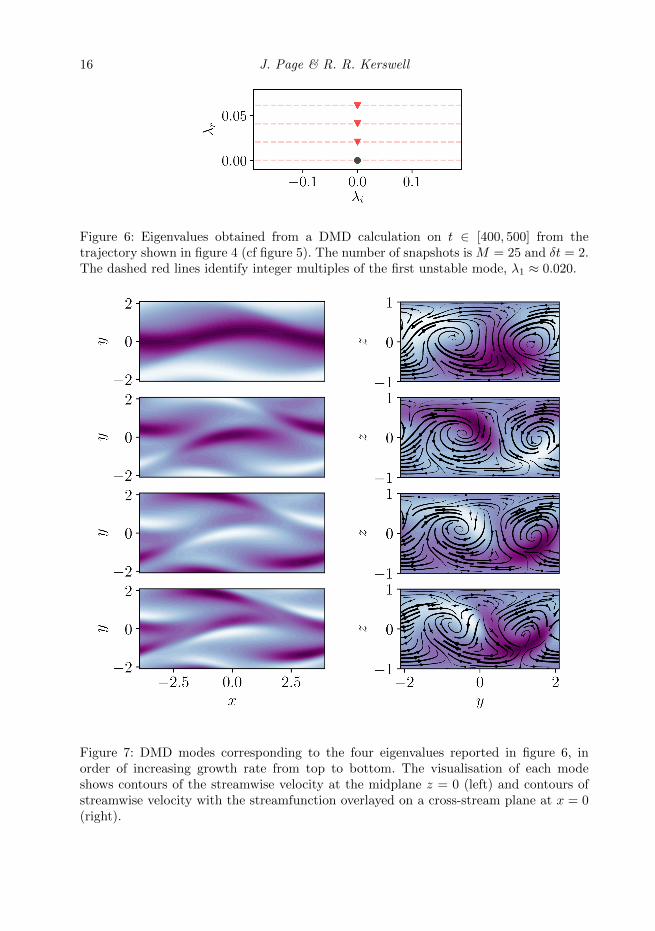
Figure 6: Eigenvalues obtained from a DMD calculation on t ∈ [400, 500] from thetrajectory shown in figure 4 (cf figure 5). The number of snapshots is M = 25 and δt = 2.The dashed red lines identify integer multiples of the first unstable mode, λ1 ≈ 0.020.
Figure 7: DMD modes corresponding to the four eigenvalues reported in figure 6, inorder of increasing growth rate from top to bottom. The visualisation of each modeshows contours of the streamwise velocity at the midplane z = 0 (left) and contours ofstreamwise velocity with the streamfunction overlayed on a cross-stream plane at x = 0(right).

Koopman expansions 17
Figure 8: Eigenvalues obtained from a DMD calculation on t ∈ [1000, 1100] from thetrajectory shown in figure 4 (cf figure 5). The number of snapshots is M = 25 andδt = 2. The dashed blue lines identify integer multiples of the slowest-decaying mode,λ1 ≈ −0.017 + 0.031i.
Figure 9: DMD modes (real part shown) corresponding to the four blue eigenvalueswith λi > 0 reported in figure 8, in order of increasing |λ| from top to bottom. Thevisualisation of each mode shows contours of the streamwise velocity at the midplanez = 0 (left) and contours of streamwise velocity with the streamfunction overlayed on across-stream plane at x = 0 (right).

18 J. Page & R. R. Kerswell
Figure 10: Error in the DMD approximation(s) (equation 3.3) versus the true evolution,ε := ‖uD − u‖/‖u‖. Red and blue lines identify approximations to the attracting andrepelling expansions respectively, the grey regions identify windows where the DMDcalculations and fitting were performed.
is actually four-dimensional. Their importance as the Reynolds number is increased isdiscussed in more detail below.
The existence of a crossover point between the two Koopman decompositions can beexplored further by using the output of the DMD calculations to construct approxima-tions to the true trajectory. To that end, we use the two DMD calculations reported infigures 6 and 8 to construct approximations to the true heteroclinic connection. We seeka low-dimensional representation of the flow from DMD, uD, by summing over a subsetV± of the DMD modes from either the repelling or attracting regions,
uD(x, t) = uC(x) +∑λj∈V
ajvj(x)eλjt. (3.3)
For each expansion, the modes in V± are exactly those reported in figure 6 and 8.For the repelling expansion, this includes the neutral mode and the three unstableeigenvalues. For the attracting expansion, the neutral mode, the five stable (blue) modesassociated with the slowest-decaying spiral and the complex-conjugate (orange) pair ofmodes associated with the second, more rapidly decaying spiral are included.
The amplitudes, {aj}, assigned to the DMD modes are determined by a least-squares fitto the true trajectory within the DMD time window. Taking M equally spaced snapshotsalong the fitting window separated by a time δt, the function to be minimised is
J(a) :=1
M
M−1∑m=0
∣∣ψ(u(x,mδt))−∑j
ajvjemλjδt
∣∣2. (3.4)
The solution to the least-squares problem for a is then
a =
(∑m
(ΛH)mVHVΛm)−1∑
m
(ΛH)mVHψ(u(x,mδt)), (3.5)
where Λ is a diagonal matrix where the ith entry is eλiδt and V is a matrix whose ith
column is the ith DMD mode.The error betweeen the repelling and attracting approximations and the true solution
are reported in figure 10. Unsurprisingly, the error in each case is smallest in the fittingwindows themselves. The error also remains vanishingly small as each expansion is pushedtowards its respective equilibrium solution, but both expansions blow up as they arepushed beyond an apparent crossover point at t ≈ 750.

Koopman expansions 19
Figure 11: DMD approximations to Koopman eigenfunctions, including their timeevolution, obtained in both the repelling (left - also see figures 6 and 7) and attracting(right - also see figures 8 and 9) regions. The DMD time window is highlighted in grey,and the dashed lines identify temporal behaviour ∼ eλjt. Note all repelling eigenfunctionsare normalised to unity at t = 400; the attracting eigenfunctions are normalised to unityat t = 1100.
In addition to computing the error against the true trajectory, an alternative way ofassessing the output of the DMD calculations in connection to the Koopman operator isto examine the numerical approximation to the Koopman eigenfunctions. As describedin §2, these objects are obtained from the left-eigenvectors of the DMD operator, {wj}as follows (Rowley & Dawson 2017),
ϕj(u) = wHj ψ(u). (3.6)
The “performance” of DMD can be examined by evaluating this inner product for pointson the trajectory beyond the DMD time window, which we do in figure 11. It is clearthat the DMD calculations on the relatively short time window Tw = 100 have been ableto accurately build locally valid representations of the Koopman eigenfunctions whichremain reasonably accurate for two to three hundred advective time units beyond theobservation window. These local approximations become increasingly poor around the“crossover point” inferred from earlier figures (e.g. 5 and 10), a behaviour which again isanalogous to DMD of the Stuart-Landau equation (e.g. figure 3).
3.2. Higher Reynolds numbers
In both the one dimensional Stuart-Landau equation (§2) and the example discussedabove at Re = 135, there are only two fixed points: repelling and attracting equilibria.This results in a pair of Koopman expansions that extend beyond the respective re-pelling/attracting linear subspaces to a crossover point in state space. Here, we increasethe Reynolds number in the Nagata box to examine the consequences for Koopmandecompositions and DMD when the structure of state space is complicated by thepresence of additional invariant sets. The motivation here is to explore the possibilityof applying DMD to turbulent trajectories as a method of locating nearby coherentstructures and their associated Koopman mode expansions.
The eigenvalue spectra obtained in figures 5 and 8 indicate that the stable subspacearound the upper branch is four-dimensional (two orthogonal spirals). The DMD alsorevealed the higher-order Koopman eigenvalues required to propagate u beyond the linearsubspace. The second, more rapidly decaying spiral (orange squares in figure 8) becomes

20 J. Page & R. R. Kerswell
Figure 12: DMD eigenvalue spectra obtained in the vicinity of uUB at Re = 140 (left) andRe = 150 (right). At Re = 140, the upper branch solution is stable and the spectrum wasobtained in a similar manner to that shown in figure 8 at Re = 135 (M = 25 snapshots ina timewindow of length Tw = 100, with δt = 2). At Re = 150, the DMD was performedon a trajectory f t(uUB) over t ∈ [0, 700), where uUB is the numerical approximationto the upper branch equilibrium converged using Newton-GMRES over a time intervalT = 4. M = 25 snapshots were used with spacing δt = 1.
increasingly dominant in the dynamics as the Reynolds number is increased. Thisbehaviour is apparent in figure 12, where we report DMD eigenvalues from trajectoriesvery close to the upper branch uUB at Re ∈ {140, 150}.
At Re = 140 the eigenvalues associated with the second spiral in the linear subspacearound uUB (λ = ζ±1 ≈= −0.015 ± 0.091i; orange in figure 12), which had only a weakeffect on the dynamics at Re = 135, have become the most slowly decaying to dominatethe linearized dynamics. In addition, higher order Koopman eigenvalues in the samefamily as ζ±1 are also obtained from the DMD (e.g. 2ζ1 associated with ϕ2
ζ1(u)) and
are highlighted with dashed lines. The decay rate of the first spiral (blue triangles) hasapproximately doubled. Note that, in addition to the two families of Koopman eigenvaluesassociated with the dynamics in the linear subspace, there are also eigenvalues which areconnected to products of Koopman eigenfunctions from these families. For example, infigure 12 the green diamonds identify eigenvalues λ±1 +ζ±1 associated with eigenfunctionsϕ±λ1
(u)ϕ±ζ1(u).At around Re ≈ 145 the complex conjugate pair of eigenvalues associated with the
dominant spiral, ζ±1 , cross the imaginary axis (not shown) to become unstable, anda stable period orbit (SPO) is born in a Hopf bifurcation off uUB . This behaviour isapparent in the results of DMD at Re = 150 in figure 12. In addition to the unstable pairof eigenvalues associated with the dynamics in the linear subspace, ζ±1 ≈ 0.007± 0.095i,higher order Koopman eigenvalues are again observed, and correspond to products of theKoopman eigenfunctions ϕ±ζ1(u).
The destabilisation of the upper branch solution and the emergence of a SPO hasfurther consequences for DMD. There are now three crossover points associated withKoopman decompositions around each of the three invariant sets (uLB , uUB and theSPO), and DMD will only “work” if it is restricted to a particular expansion zone. Theresults highlight the care that must be taken in more complex flows with many exactcoherent states buried in the turbulent attractor.
To demonstrate the restrictions placed on DMD, we consider again a trajectorybeginning in the linear subspace around uLB , which now collapses into the SPO as t→∞.Similar to our approach for the uLB → uUB connection at Re = 135, we perform manyDMDs in a fixed time window which is passed along the finite time approximation to the

Koopman expansions 21
Figure 13: (Top) Imaginary and (bottom) real components of DMD eigenvalues obtainedon shorter time windows passed through a trajectory running from the linear subspace ofuLB to the SPO at Re = 150 (the variable tF is the “final” time of each time window).Left: time windows of length Tw = 50 are used with M = 50 snapshots. Right: Tw = 200with M = 150 snapshots. Snapshot spacing is δt = 1 for both sets of calculations. Thecolouring serves as a guide for the eye, with red, orange and blue identifying expansionsaround uLB , uUB and the SPO respectively.
Figure 14: DMD eigenvalues obtained from the uLB → SPO heteroclinic connection atRe = 150. Left: time window t ∈ [450, 500], with M = 50 snapshots, δt = 1 (c.f. upperbranch spectrum in 12). Right: time window t ∈ [650, 1000], with M = 200 snapshots,δt = 1. The modes highlighted in green are the Floquet multipliers µ ≈ −0.017± 0.026i(from the form eµδt). Dashed lines identify harmonics of the fundamental frequency ofthe periodic orbit.
heteroclinic connection. The results of these calculations for two DMD time windows,Tw ∈ {50, 200}, are reported in figure 13.
For the shorter DMD time window, Tw = 50, three distinct trends in the eigenvalues areobserved. As the trajectory moves away from the lower branch solution, the DMD locatesthe positive, real eigenvalue associated with the growth rate along the single unstabledirection, before identifying the integer multiples of this growth rate corresponding to thehigher order Koopman modes. This behaviour is analogous to that found at Re = 135(see figure 5); like that earlier uLB → uUB connection, there is also a breakdown in theDMD/Koopman eigenvalues, here at tF ∼ 400. The region where there is inconsistency

22 J. Page & R. R. Kerswell
between successive DMD calculations is roughly twice the length of the DMD timewindow, which suggests the presence of a crossover point. Beyond tF ∼ 450, there isa clear repeated frequency in the DMD eigenvalues, λi ≈ 0.064, consistent over roughly100 advective time units. This frequency is close to that associated with the stable spiralinto the upper branch (λi = 0.069, see figure 12). However, the DMD is unable to resolvethe associated decay rate correctly, or obtain the complex conjugate pair of unstablemodes associated with uUB at this Reynolds number. An individual eigenvalue spectrumfrom this region is reported in figure 14 and should be contrasted with those obtainedon trajectories starting in the linear subspace of uUB (figure 12). A pair of unstableeigenvalues are found, though their growth rate and frequency do not correspond to theunstable directions identified in figure 12. It is likely that the trajectory simply does notgo close enough to the upper branch equilibrium to accurately distinguish the correctform of the neutral mode (uUB itself) from the slowly growing eigenvalues, and this errorcontaminates the rest of the spectrum. Finally, at around tF ∼ 600 the output of theDMD calculations jumps again. There are clear repeated harmonics of a fundamentalfrequency, ωf = 0.085 (λr is very close to zero), which corresponds to a periodic orbitwith period T = 73.9. Occasionally, the DMD erroneously identifies growing modes,while the lattice of decaying eigenvalues one would expect to find around a stable limitcycle is absent (e.g. as observed by Bagheri (2013) and proven for systems with a singleattracting limit cycle by Mezic (2017)).
To accurately determine the Koopman eigenvalues around the SPO, a much longer timewindow is required. For example, the longer time window considered in figure 13, Tw =200, no longer shows exponentially unstable modes in the collapse onto the SPO. Instead,there is an array of decaying eigenvalues, all with decay rate λr ≈ −0.017. Each harmonicof the SPO is flanked by a pair of decaying modes, λ = nωf i + (µr ± µii), indicatingthe presence of a pair of stable Floquet multipliers eµT , with µ = −0.017 ± 0.026i. Toobtain higher order Koopman modes associated with the SPO (see Bagheri 2013), evenlonger time windows are required. For example, the decay rate 2µr is observed in figure14 with a slightly longer time window Tw = 350, although only approximately and thereare eigenvalues missing.
A consequence of the longer time window required for a more accurate resolution ofthe Koopman eigenvalues around the SPO is the loss of any indication of the presence ofthe upper branch in figure 13. The time window is longer than the residence time in theupper branch expansion region, so all DMD calculations that see uUB contain at least onecrossover point. In addition to a large time window, Tw > T , DMD calculations whichare able to accurately resolve the Koopman eigenvalues around the periodic orbit requiremany snapshot pairs. In a turbulent flow with unstable periodic orbits (UPOs), each withmany different Floquet multipliers, these requirements are unlikely to be achievable inpractice. However, the fact that DMD time windows which are shorted than the period,Tw < T , are still able to identify the fundamental frequencies and associated mode shapesindicates that DMD may be a useful alternative to a recurrent flow analysis in generatingguesses for UPOs.
4. Conclusion
In this paper we have examined how the presence of multiple simple invariant solutionsin a nonlinear dynamical system affects the construction of Koopman expansions forthe state variable. We showed how an inverse Laplace transform can be used to obtainKoopman mode decompositions if the Koopman eigenvalues are purely real, before ap-plying this technique to the Stuart-Landau equation. The solution revealed two possible

Koopman expansions 23
Koopman expansions, each corresponding to a particular fixed point of the dynamicalsystem. There is a crossover point in state space where one expansion breaks down andthe other takes over. The success of DMD in locating Koopman eigenvalues dependscritically on the location of the crossover point: a DMD performed over a time windowwhich contains the crossover point will fail. Instead DMD then returns a fragile (sensitiveto the time window used) best fit of the dynamics to exponential terms unrelated to theunderlying Koopman operator.
We then applied DMD to some heteroclinic connections of the Navier-Stokes equationsin Couette flow at low Reynolds number. The results confirm the existence of a differentKoopman expansion around each simple invariant solution. Again, the ability of DMDto discover these decompositions is constrained by the presence of crossover points inphase space. Only a DMD restricted to a particular “expansion region” can identify theunderlying Koopman eigenvalues and modes. These results suggest that in a dynamicalsystem possessing multiple simple invariant solutions, there are generically places in phasespace – plausibly hypersurfaces delineating the boundary of a local Koopman expansion– across which the dynamics cannot be represented by a convergent Koopman expansion.
An interesting open question is then how Koopman decompositions which are ableto represent a general orbit in a turbulent attractor, i.e. one built from harmonicaverages at discrete frequencies and featuring a continuous spectrum, is related to theindividual Koopman expansions about the simple invariant sets which form a skeletonfor the overall dynamics. What is clear is that DMD applied to arbitrary turbulenttrajectories will not necessarily yield Koopman modes and eigenvalues associated witheither approach. However, our results suggest that DMD may still be a useful tool forfinding exact coherent structures near to a turbulent orbit provided the data window istaken small enough so that only the neighbourhood of one coherent structure is sampled.The approach when searching for equilibria is more refined than supplying snapshotsof the turbulent field and trying to converge a steady solution with GMRES-Hookstep.While for periodic orbits, the DMD time window need not contain a “near recurrence” toidentify the relevant frequencies and mode shapes that serve as the input to a root-findingalgorithm. We hope to report our results using DMD to extract coherent structures fromturbulent flows in the very near future.
Appendix: Carleman linearization
In this appendix, we show that the two Koopman expansions found in §2.3 emergenaturally from Carleman linearization about the respective equilibria. The 1D nonlinearequation (2.8) can be converted into an infinite dimensional linear system
dxndt
= (2n− 1)(xn − xn+1) (4.1)
by defining new variables xn := R2n−1(t) for n ∈ N. A truncated version of this system(xn = 0 for n > N) should approximate the dynamics in the neighbourhood of theequilibria R = 0 where neglected variables should be negligible. This truncated systemis
dx
dt= Lx (4.2)
where x = (x1 x2 . . . xN )T and Lnn = 2n − 1, Lnn+1 = −(2n − 1) with Lnm = 0otherwise. The matrix L is (upper) triangular so its eigenvalues can be read off from thediagonal and correspond to the first N Koopman eigenvalues relevant for an expansionaround r = 0. The left eigenvector w(n) of the eigenvalue 2n − 1 corresponds to the
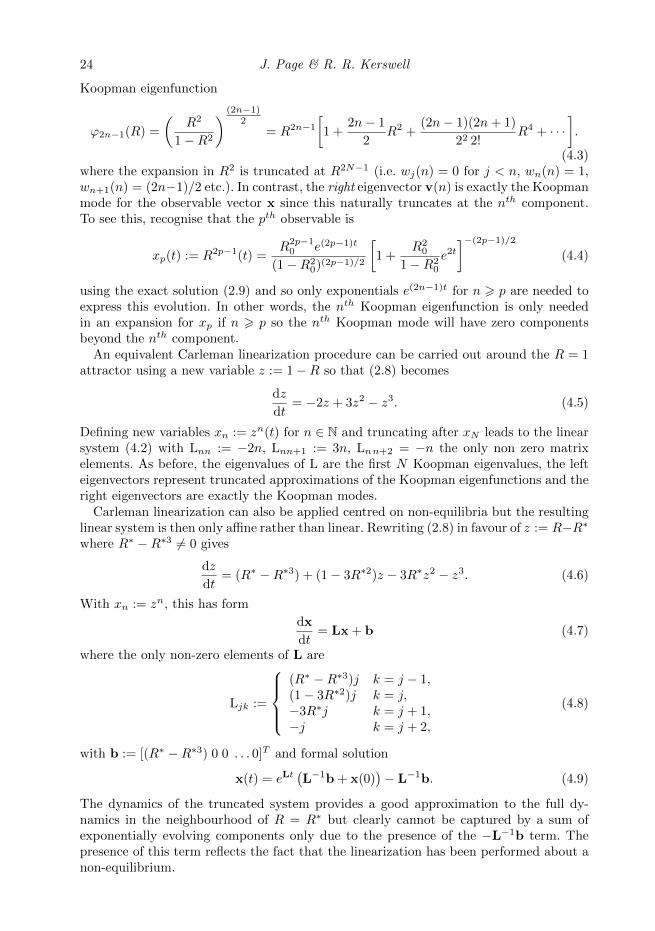
24 J. Page & R. R. Kerswell
Koopman eigenfunction
ϕ2n−1(R) =
(R2
1−R2
) (2n−1)2
= R2n−1[1 +
2n− 1
2R2 +
(2n− 1)(2n+ 1)
22 2!R4 + · · ·
].
(4.3)where the expansion in R2 is truncated at R2N−1 (i.e. wj(n) = 0 for j < n, wn(n) = 1,wn+1(n) = (2n−1)/2 etc.). In contrast, the right eigenvector v(n) is exactly the Koopmanmode for the observable vector x since this naturally truncates at the nth component.To see this, recognise that the pth observable is
xp(t) := R2p−1(t) =R2p−1
0 e(2p−1)t
(1−R20)(2p−1)/2
[1 +
R20
1−R20
e2t]−(2p−1)/2
(4.4)
using the exact solution (2.9) and so only exponentials e(2n−1)t for n > p are needed toexpress this evolution. In other words, the nth Koopman eigenfunction is only neededin an expansion for xp if n > p so the nth Koopman mode will have zero componentsbeyond the nth component.
An equivalent Carleman linearization procedure can be carried out around the R = 1attractor using a new variable z := 1−R so that (2.8) becomes
dz
dt= −2z + 3z2 − z3. (4.5)
Defining new variables xn := zn(t) for n ∈ N and truncating after xN leads to the linearsystem (4.2) with Lnn := −2n, Lnn+1 := 3n, Lnn+2 = −n the only non zero matrixelements. As before, the eigenvalues of L are the first N Koopman eigenvalues, the lefteigenvectors represent truncated approximations of the Koopman eigenfunctions and theright eigenvectors are exactly the Koopman modes.
Carleman linearization can also be applied centred on non-equilibria but the resultinglinear system is then only affine rather than linear. Rewriting (2.8) in favour of z := R−R∗where R∗ −R∗3 6= 0 gives
dz
dt= (R∗ −R∗3) + (1− 3R∗2)z − 3R∗z2 − z3. (4.6)
With xn := zn, this has form
dx
dt= Lx + b (4.7)
where the only non-zero elements of L are
Ljk :=
(R∗ −R∗3)j k = j − 1,(1− 3R∗2)j k = j,−3R∗j k = j + 1,−j k = j + 2,
(4.8)
with b := [(R∗ −R∗3) 0 0 . . . 0]T and formal solution
x(t) = eLt(L−1b + x(0)
)− L−1b. (4.9)
The dynamics of the truncated system provides a good approximation to the full dy-namics in the neighbourhood of R = R∗ but clearly cannot be captured by a sum ofexponentially evolving components only due to the presence of the −L−1b term. Thepresence of this term reflects the fact that the linearization has been performed about anon-equilibrium.

Koopman expansions 25
REFERENCES
Ahmed, M. A. & Sharma, A. S. 2017 New equilibrium solution branches of plane Couetteflow discovered using a project-then-search method. arXiv 1706.05312 .
Arbabi, H. & Mezic, I. 2017 Study of dynamics in post-transient flows using Koopman modedecomposition. Phys. Rev. Fluids 2, 124402.
Avila, M., Mellibovsky, F., Roland, N. & Hof, B. 2013 Streamwise-localized solutions atthe onset of turbulence in pipe flow. Physical Review Letters 110, 224502.
Bagheri, S. 2013 Koopman-mode decomposition of the cylinder wake. J. Fluid Mech. 726,596–623.
Brand, E. & Gibson, J. F. 2014 A doubly localized equilibrium solution of plane Couetteflow. Journal of Fluid Mechanics 750, R3.
Brunton, B. W., Johnson, L. A., Ojemann, J. G. & Kutz, J. N. 2016a Extractingspatial–temporal coherent patterns in large-scale neural recordings using dynamic modedecomposition. Journal of Neuroscience Methods 258, 1–15.
Brunton, S. L., Brunton, B. W., Proctor, J. L. & Kutz, J. N. 2016b Koopman invariantsubspaces and finite linear repesentations of nonlinear dynamical systems for control.PLoS ONE 11 (2).
Carleman, T. 1932 Application de la theories des equations integrales lineaires aux systemesd’equations differentielles non lineaires. Acta. Math. 59, 63–87.
Chandler, G. J. & Kerswell, R. R. 2013 Invariant recurrent solutions embedded in aturbulent two-dimensional kolmogorov flow. Journal of Fluid Mechanics 722, 554–595.
Chantry, M, Willis, A. P. & Kerswell, R. R. 2014 Genesis of streamwise-localised solutionsfrom globally periodic traveling waves in pipe flow . Physical Review Letters 112, 164501.
Cvitanovic, P. & Gibson, J. F. 2010 Geometry of the turbulence in wall-bounded shearflows: periodic orbits . Physica Scripta T142, 014007.
Deguchi, K. 2017 Scaling of small vortices in stably stratified shear flows . Journal of FluidMechanics 821, 582–594.
Eaves, T. S., Caulfield, C. P. & Mezic, I. 2016 Transition to Turbulence:highway through the edge of chaos is charted by Koopman modes. APS Bulletinhttp://meetings.aps.org/link/BAPS.2016.DFD.D8.3.
Eckhardt, B., Schneider, T. M., Hof, B. & Westerweel, J. 2007 Turbulence transitionin pipe flow . Annual Review of Fluid Mechanics 39, 447–468.
Faisst, H. & Eckhardt, B. 2003 Traveling waves in pipe flow . Physical Review Letters 91,224502.
Gaspard, P. 1998 Chaos, Scattering and Statistical Mechanics, 1st edn. Cambridge UniversityPress.
Gaspard, P., Nicolis, G., Provata, A. & Tasaki, S. 1995 Spectral signature of the pitchforkbifurcation: Liouville equation approach. Physical Review E 51, 74.
Gibson, J. F. & Brand, E. 2014 Spanwise-localized solutions of planar shear flows. Journalof Fluid Mechanics 745, 25–61.
Gibson, J. F., Halcrow, J. & Cvitanovic, P. 2008 Visualizing the geometry of state spacein plane couette flow. Journal of Fluid Mechanics 611, 107–130.
Gibson, J. F., Halcrow, J. & Cvitanovic, P. 2009 Equilibrium and travelling-wave solutionsof plane couette flow. Journal of Fluid Mechanics 638, 243–266.
Hall, P. & Sherwin, S. 2010 Streamwise vortices in shear flows: harbingers of transition andthe skeleton of coherent structures. Journal of Fluid Mechanics 661, 178–205.
Hamilton, J. M., Kim, J. & Waleffe, F. 1995 Regeneration mechanisms of near-wallturbulence structures. Journal of Fluid Mechanics 287, 317–348.
Jovanovic, M. R., Schmid, P. J. & Nichols, J. W. 2014 Sparsity-promoting dynamic modedecomposition. Phys. Fluids 26, 024103.
Kawahara, G. & Kida, S. 2001 Periodic motion embedded in plane couette turbulence:regeneration cycle and burst. Journal of Fluid Mechanics 449, 291–300.
Kawahara, G., Uhlmann, M. & van Veen, L. 2012 The significance of simple invariantsolutions in turbulent flows. Annual Review of Fluid Mechanics 44 (1), 203–225.
Kerswell, R. R. 2005 Recent progress in understanding the transition to turbulence in a pipe.Nonlinearity 18, R17–R44.
26 J. Page & R. R. Kerswell
Koopman, B. O. 1931 Hamiltonian Systems and Transformations in Hilbert Space. Proc. Nat.Acad. Sci. 17 (5), 315–318.
Kutz, J. N., Brunton, S. L., Brunton, B. W. & Proctor, J. L. 2016a Dynamic ModeDecomposition: Data-Driven Modeling of Complex Systems, 1st edn. SIAM.
Kutz, J. N., Fu, X. & Brunton, S. L. 2016b Multiresolution dynamic mode decomposition.SIAM Journal on Applied Dynamical Systems 15, 713–735.
Lucas, D., Caulfield, C. P. & Kerswell, R. R. 2017 Layer formation in horizontally forcedstratified turbulence: connecting exact coherent structures to linear instabilities. Journalof Fluid Mechanics 832, 409–437.
Lusch, B., Kutz, J. N. & Brunton, S. L. 2018 Deep learning for universal linear embeddingsof nonlinear dynamics. arXiv 1712.09707 .
Mezic, I. 2005 Spectral Properties of Dynamical Systems, Model Reduction andDecompositions. Nonlinear Dynam. 41, 309–325.
Mezic, I. 2013 Analysis of Fluid Flows via Spectral Properties of the Koopman Operator. Ann.Rev. Fluid Mech. 45, 357–378.
Mezic, I. 2017 Koopman Operator Spectrum and Data Analysis. arXiv 1702.07597 .Mezic, I. & Banaszuk, A. 2004 Comparison of systems with complex behavior. Physica D
197, 101–133.Nagata, M. 1990 Three-dimensional finite-amplitude solutions in plane couette flow: bifurcation
from infinity. Journal of Fluid Mechanics 217, 519–527.Olvera, D. & Kerswell, R. R. 2017 Exact coherent structures in stably stratified plane
couette flow. Journal of Fluid Mechanics 826, 583–614.Page, J. & Kerswell, R. R. 2018 Koopman analysis of Burgers equation. Physical Review
Fluids 3, 071901(R).Rowley, C. W. & Dawson, S. T. M. 2017 Model Reduction for Flow Analysis and Control.
Ann. Rev. Fluid Mech. 49, 387–417.Rowley, C. W., Mezic, I., Bagheri, S., Schlatter, P. & Henningson, D. S. 2009 Spectral
analysis of nonlinear flows. J. Fluid Mech. 641, 115–127.Schmid, P. J. 2010 Dynamic mode decomposition of numerical and experimental data. J. Fluid
Mech. 656, 5–28.Schneider, T. M., Eckhardt, B. & Yorke, J. A. 2007 Turbulence transition and the edge
of chaos in pipe flow. Physical Review Letters 99, 034502.Schneider, T. M., Gibson, J. F. & Burke, J. 2010 Snakes and ladders: Localized solutions
of plane couette flow. Physical Review Letters 104, 104501.Sharma, A. S., Mezic, I. & McKeon, B. J. 2016 Correspondence between Koopman mode
decompositions, resolvent mode decomposition and invariant solutions of the Navier-Stokes equations. Phys. Rev. Fluids 1, 032402(R).
Tu, J. H, Rowley, C. W., Luchtenburg, D. M., Brunton, S. L. & Kutz, J. N. 2014On dynamic mode decomposition: theory and applications. J. Comput. Dynam. 1 (2),391–421.
Uhlmann, M., Kawahara, G. & Pinelli, A. 2010 Traveling-waves consistent with turbulence-driven secondary flow in a square duct. Physics of Fluids 22 (8), 084102.
Viswanath, D. 2007 Recurrent motions within plane couette turbulence. Journal of FluidMechanics 580, 339–358.
Waleffe, F. 1997 On a self-sustaining process in shear flows. Physics of Fluids 9, 883–900.Waleffe, F. 2001 Exact coherent structures in channel flow. Journal of Fluid Mechanics 435,
93–102.Wang, J., Gibson, J. & Waleffe, F. 2007 Lower branch coherent states in shear flows:
Transition and control. Physical Review Letters 98, 204501.Wedin, H. & Kerswell, R.R. 2004 Exact coherent structures in pipe flow: travelling wave
solutions. Journal of Fluid Mechanics 508, 333–371.Williams, M. O., Kevrekidis, I. G. & Rowley, C. W. 2015 A Data-Driven Approximation
of the Koopman Operator: Extending Dynamic Mode Decomposition. J. Nonlinear Sci.25 (6), 1307–1346.
Zammert, S. & Eckhardt, B. 2014 Streamwise and doubly-localized periodic orbits in planePoiseuille flow. Journal of Fluid Mechanics 761, 348–359.