Konstantin Meyl

Scalar waves

From an extended vo rtex and field theory to a technical, b io logical and historical use of longitudinal w aves.

Edition belonging to the lecture and sem in ar „E lectromagnetic E nv ironm enta l C o m pa tib il ity ”

Edition be longing to the se m in a r (part 1 - 3 ) „E lec trom agne tic E nv ironm en ta l C o m p a tib il i ty ” by Prof. Dr. Konstantin Meyl

From Maxwell's field equations only the well-known (transverse) Hertzian waves can

be derived, whereas the calculation of longitudinal scalar waves gives zero as a result.

This is a flaw of the field theory, since scalar waves exist for all particle waves, like e.g.

as plasma wave, as photon- or neutrino radiation. Starting from Faraday's discovery,

instead of the formulation of the law of induction according to Maxwell, an extended field theory is derived, which goes beyond the Maxwell theory with the description of

potential vortices (noise vortices) and their propagation as a scalar wave, but contains the Maxwell theory as a special case. With that the extension is allowed and doesn't

contradict textbook physics.

Besides the mathematical calculation of scalar waves this book contains a voluminous

material collection concerning the information technical use of scalar waves, if the

useful signal and the usually interfering noise signal change their places, if a separate

modulation of frequency and wavelength makes a parallel image transmission

possible, if it concerns questions of the environmental compatibility for the sake of humanity (bio resonance, among others) orto harm humanity (electro smog).

From an extended vortex and field theory to a technical, b iological and historical use of longitudinal w aves.

INDEL G m bH, V erlagsabte ilung ISBN 3-9802542-4-0

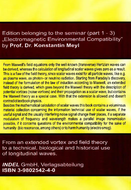
480 Neutrino radiation

V » C

hard neutrino radiation(small ring-like vortex)

weak neutrino radiation(large ring-like vortex)

photon radiation (light = individual ring-like vortex or

as an oscillating pair).

plasma waves, noise,earth radiation

(vortex balls, consisting of a multitude of ring-like vortices).

Fig. 22.5: The ring-like vortex model of scalar waves.

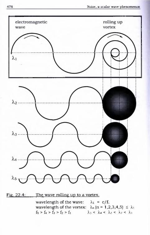
478 Noise, a scalar wave phenomenon

A.5

Fig. 22.4:_____ The wave rolling up to a vortex.

wavelength of the wave: A,i = c/fi wavelength of the vortex: A,n (n = 1,2,3,4,5) < A.ifs > ft > i? > f2 > fl X,5 < ^.4 < .̂3 < A.2 < A,1

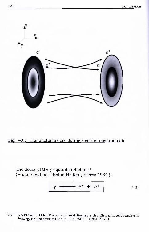
62 pair creation

Fig. 4.6: The photon as oscillating electron-positron pair

The decay of the y - quanta (photon)<j>( = pair creation = Bethe-Heitler-process 1934 ):

y ------ - e~ + e+ (4.2)

<i> Nachtmann, Otto: Phänomene und Konzepte der Elementarteilchenphysik, Vieweg, Braunschweig 1986, S. 135, ISBN 3-528-08926-1

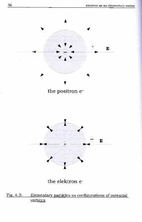
56 electron as an elementary vortex

> " A,

f

the positron e+

s !-— - +

/ ! s

the elektron e-

Fig. 4.3: Elementary particles as configurations of potential vortices

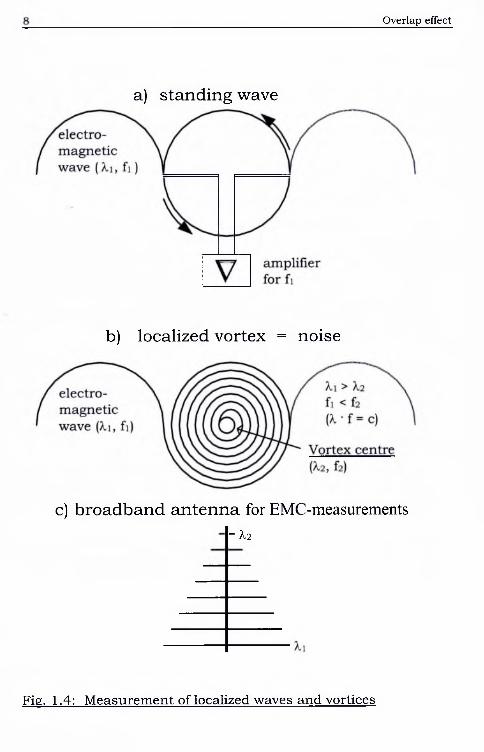
Overlap effect

a) standing wave

b) localized vortex = noise

c) broadband antenna for EMC-measurements“ X2

Fig. 1.4: Measurement of localized waves and vortices

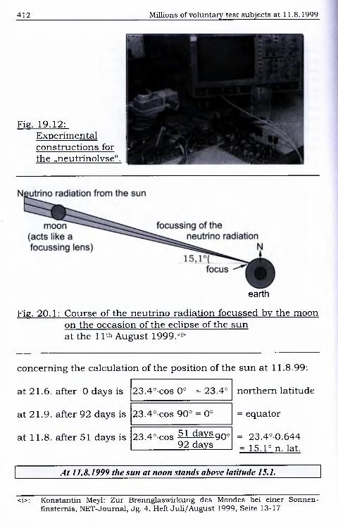
412 Millions of voluntary test subjects at 11.8.1999

Fig. 19.12:Experimental constructions for the „neutrinolyse“.

earth

Fig. 20.1: Course of the neutrino radiation focussed by the moon on the occasion of the eclipse of the sun at the 11th August 1999.<i>

concerning the calculation of the position of the sun at 11.8.99:

northern latitudeat 21.6. after 0 days is

at 21.9. after 92 days is

at 11.8. after 51 days is

23.4° cos 0° = 23.4°

23.4° cos 90° = 0°

23.4° cos 51 daYS.9 0c __________ 92 days

= equator

= 23.4°0.644 = 15.1° n. lat.

At 11.8.1999 the sun at noon stands above latitude 15.1.

<i>: Konstantin Meyl: Zur Brennglaswirkung des Mondes bei einer Sonnen­finsternis, NET-Journal, Jg. 4, Heft Juli/August 1999, Seite 13-17

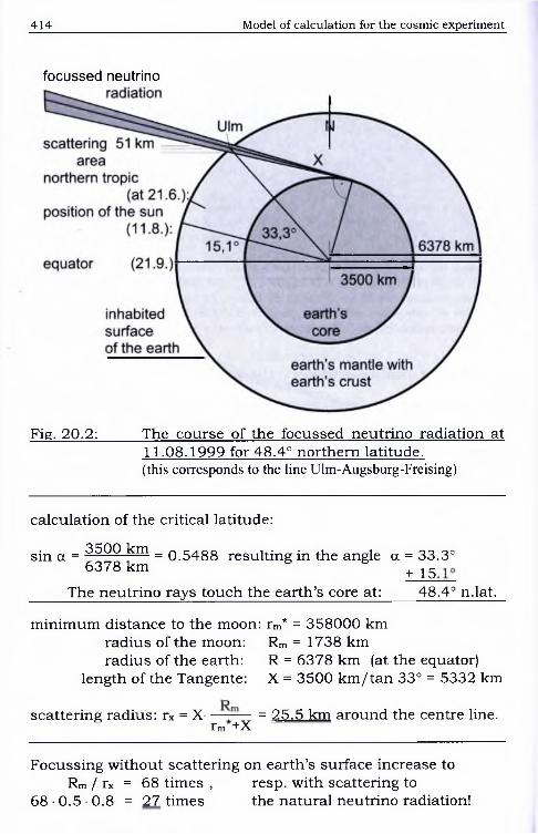
414 Model o f calculation for the cosmic experiment

focussed neutrino

Fig. 20.2:______ The course of the focussed neutrino radiation at11.08.1999 for 48.4° northern latitude.(this corresponds to the line Ulm-Augsburg-Freising)

calculation o f the critical latitude:

sin a = 3500 km = 0.5488 resulting in the angle a = 33.3° 6378 km + ^

_____ The neutrino rays touch the earth’s core at:_____ 48.4° n.lat.

minimum distance to the moon: rm* = 358000 km radius of the moon: Rm = 1738 km radius of the earth: R = 6378 km (at the equator)

length o f the Tangente: X = 3500 km/tan 33° = 5332 km

scattering radius: rx = X- — — = 25.5 km around the centre line.Tm +X

Focussing without scattering on earth’s surface increase to Rm / rx = 68 times , resp. with scattering to

68 • 0.5 ■ 0.8 = 27 times the natural neutrino radiation!

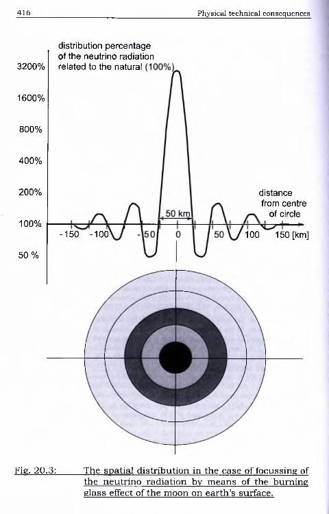
416 Physical technical consequences

3200%

1600%

800%

400%

200%

100%

50 %

distribution percentage of the neutrino radiation related to the natural '

distance from centre

of circle

150 [km]-150 -100 100

Fig. 20.3:______ The spatial distribution in the case of focussing ofthe neutrino radiation by means of the burningglass effect of the moon on earth’s surface.

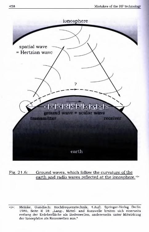
458 Mistakes of the HF technology

spatial wave - Hertzian wave

WMWWWMMWhground wave = scalar wave

transmitter

ionosphere

earth

Fig. 21.6: Ground waves, which follow the curvature of theearth and radio waves reflected at the ionosphere.<i:>

<i>: Meinke, Gundlach: Hochfrequenztechnik, 4.Aufl. Springer-Verlag Berlin 1986, Seite R 18: „Lang-, Mittel- and Kurzwelle breiten sich einerseits entlang der Erdoberfläche als Bodenwellen, andererseits unter Mitwirkung der Ionosphäre als Raumwellen aus.“

464 Transition to the far-field

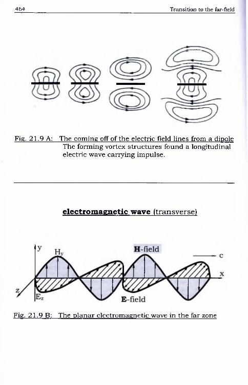
Fig. 21.9 A: The coming off o f the electric field lines from a dipole The forming vortex structures found a longitudinal electric wave cariying impulse.

electromagnetic wave (transverse)

Fig. 21.9 B: The planar electromagnetic wave in the far zone

466 Scalar wave model

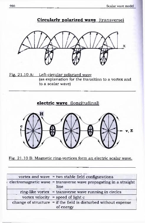
Circularly polarized wave (transverse)

Fig. 21.10 A: Left-circular polarized wave(as explanation for the transition to a vortex and to a scalar wave)

electric wave (longitudinal)

v, E

Fig. 21.10 B: Magnetic ring-vortices form an electric scalar wave.

vortex and wave = two stable field configurationselectromagnetic wave = transverse wave propagating in a straight

linering-like vortex = transverse wave running in circlesvortex velocity = speed of light c

change o f structure = if the field is disturbed without expense o f energy

468 Double-frequent oscillation of size

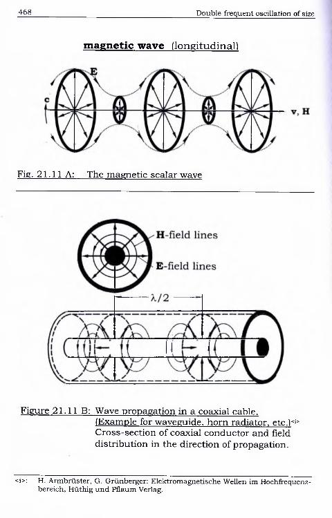
magnetic wave (longitudinal)

Fig. 21.11 A: The magnetic scalar wave

Figure 21.11 B: Wave propagation in a coaxial cable.(Example for waveguide, horn radiator. etc.)<j> Cross-section of coaxial conductor and field distribution in the direction of propagation.

<i>: H. Armbrüster, G. Grünberger: Elektromagnetische Wellen im Hochfrequenz­bereich, Hüthig und Pflaum Verlag.

470 Electric and magnetic scalar wave

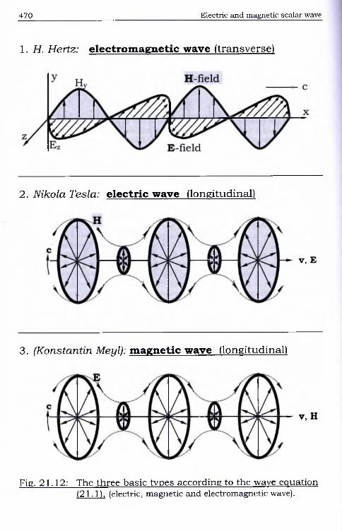
1. H. Hertz: electromagnetic wave (transverse)

2. Nikola Tesla: electric wave (longitudinal)

V, E

3. (Konstantin Meyl): magnetic wave (longitudinal)

V, H

Fig. 21.12: The three basic types according to the wave equation (21.1). (electric, magnetic and electromagnetic wave).

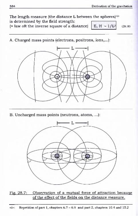
584 Derivation o f the gravitation

The length measure (the distance L between the spheres)**’is determined by the field strength: -----------------(= law oft the inverse square o f a distance) E, H ~ 1/L2 (28. 18)

A. Charged mass points (electrons, positrons, ions,...):

Fig. 28.7: Observation of a mutual force of attraction because o f the effect o f the fields on the distance measure.

<i>: Repetition of part 1, chapters 6.7 - 6.9 and part 2, chapters 10.4 and 15.2

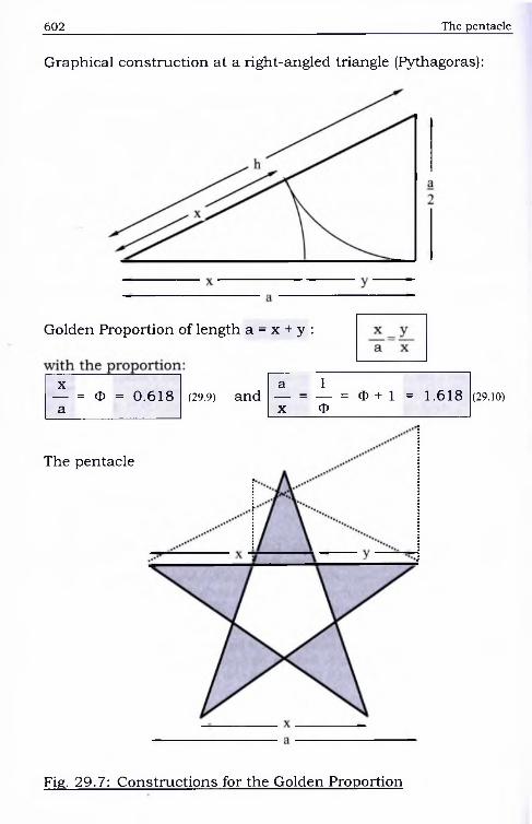
602 The pentacle

Graphical construction at a right-angled triangle (Pythagoras):

Golden Proportion of length a = x + y :

X a 1_ = CD = 0.618 (29.9) and _ = _ = $ + 1 = 1.618a x tf>

(29.10)

The pentacle

Fig. 29.7: Constructions for the Golden Proportion

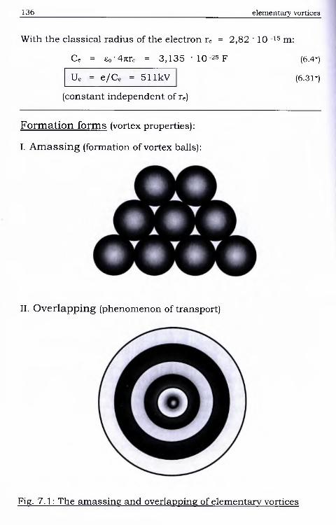
136 elementary vortices

Ue = e/Ce = 51lkV

Form ation form s (vortex properties):

I. A m ass in g (formation of vortex balls):

With the classical radius of the electron re = 2,82 ' 10

Ce = So ’ 47tre = 3,135 ■ 10 25 F

(constant independent of re)

15 m:

(6.4*)

(6.31*)

II. O verlapp in g (phenomenon of transport)

Fig. 7.1: The amassing and overlapping of elementary vortices

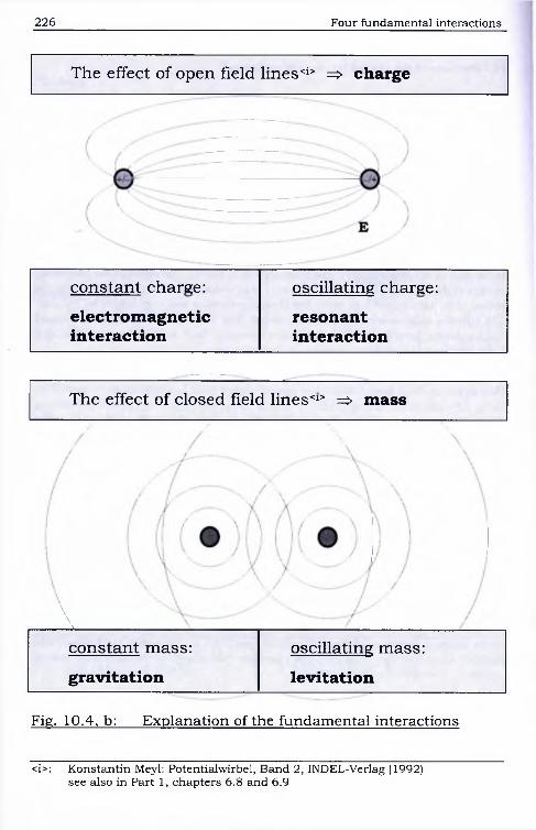
226 Four fundamental interactions

The effect of open field lines<i:> => charge

constant charge: oscillating charge:

electromagnetic resonantinteraction interaction

The effect of closed field lines*** => mass

\------->___________constant mass: oscillating mass:

gravitation levitation

Fig. 10.4, b: Explanation of the fundamental interactions

<i>: Konstantin Meyl: Potentialwirbel, Band 2, INDEL-Verlag (1992) see also in Part 1, chapters 6.8 and 6.9

228 resonant interaction

Example: central star Sz with 3 planets P 1-P3

and with 4 neighbouring stars S 1-S4

milky way-radius: 15000pc-3-109 = 45-1016km sun system-radius: 50a-15-107 = 7 ,5109 km

45-10167,5-109 1.27-10® the resonant interaction is more than eight

decimal powers bigger than the gravitation.

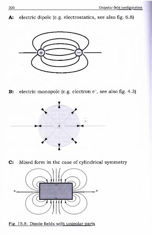
320 Unipolar field configuration

A: electric dipole (e.g. electrostatics, see also fig. 6.8)

B: electric monopole (e.g. electron e , see also fig. 4.3)

+

C: Mixed form in the case of cylindrical symmetry

Fig. 15.8: Dipole fields with unipolar parts

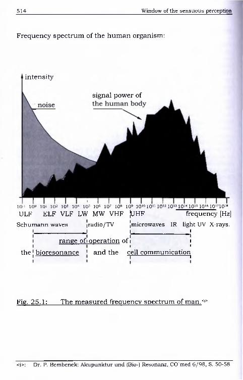
514 Window of the sensuous perception

Frequency spectrum of the human organism:

intensity

signal power of

frequency [Hz]10-' 10° 101 102 103 104 105 106 107 10s 109 101010u 1012 1013 1014 1015 1016 10>710>8

ULF ELF VLF LW MW VHF ¡UHF

Schumann waves |radio/TV ¡microwaves IR light UV X-rays. _______________ . j I___________ I

the

range ofioperation of!

bioresonance ! and the

---------------II

cell communication ~ i---------------------------------- 1

Fig. 25.1: The measured frequency spectrum of man.*1*

<i>: Dr. P. Bembenek: Akupunktur und (Bio-) Resonanz, CO'med 6/98, S. 50-58