CENTRAL BANK POLICY ANNOUNCEMENTS AND CHANGES IN TRADING

BEHAVIOR: EVIDENCE FROM BOND FUTURES HIGH FREQUENCY PRICE DATA＊

Koichiro Kamada†; Tetsuo Kurosaki‡; Ko Miura§; and Tetsuya Yamada¶

March 2018

Abstract

We present a theoretical model to explain how financial traders incorporate public and

private information into security prices. One of the remarkable features of the model is

its ability to identify simultaneously when surprising public information arrived and

how large an impact it had on the market. By applying the model to the tick-by-tick

data on Japanese bond futures prices, we show that the Bank of Japan’s introduction of

quantitative and qualitative monetary easing was one of the most surprising episodes

during the period from 2005 to 2016. We also study the sensitivity of Japanese bond

futures markets to new information. The analysis shows that the sensitivity to the

Bank’s announcements has strengthened since the introduction of the negative interest

rate policy, whereas the sensitivity to economic indicators and surveys has weakened

substantially.

Keywords: Central bank; Government bond futures; Herding behavior; Information;

Market microstructure; Policy announcements

JEL classification: C14, D40, D83, E58, G12, G14

＊ This is a preliminary draft. Please do not cite or circulate without the authors’ permission. The authors would like to thank Sergio Mayordomo Gomez, Makoto Nirei, Yosuke Takeda, the participants in the Financial Workshop held at the Bank of Japan on April 19, 2017, the 16th International Conference on Credit Risk Evaluation Designed for Institutional Targeting in finance on September 28–29, 2017, and the BOJ/IMES–BOK/ERI Workshop on December 5, 2017, and the staff of the Bank of Japan for their helpful comments and discussion. Views expressed in this paper are those of the authors and do not necessarily reflect the official views of the Bank of Japan.

† Institute for Monetary and Economic Studies, Bank of Japan: kouichirou.kamada@boj.or.jp ‡ Institute for Monetary and Economic Studies, Bank of Japan: tetsuo.kurosaki@boj.or.jp § Research and Statistics Department, Bank of Japan (currently, University of Wisconsin-Madison) ¶ Institute for Monetary and Economic Studies (currently, Financial System and Bank Examination Department), Bank of Japan: tetsuya.yamada@boj.or.jp

1

1. INTRODUCTION

Since the 1990s, the Bank of Japan (BOJ) has introduced innovative monetary policy

measures to achieve economic and financial stability in Japan. Particularly since 2013,

under the command of Governor Kuroda, the BOJ made four large policy changes to

combat long-lasting deflation and to raise inflation rates to its target rate of two

percent: quantitative and qualitative monetary easing (QQE I) on April 4, 2013; its

expansion (QQE II) on October 31, 2014; the introduction of the negative interest rate

(NIR) policy on January 29, 2016; and the launching of yield curve control (YCC) on

September 21, 2016 (see Bank of Japan, 2013, 2014, 2016a, 2016b for the related

statements). A common strategy taken in these policies is to lower and stabilize bond

yields, particularly those on long-term bonds, around an appropriate level through

various policy measures such as large-scale purchases of government bonds. These

policies had a substantial impact on financial markets. In particular, the impact of the

introduction of quantitative and qualitative monetary easing was so large that the

circuit breakers were triggered twice in the bond futures market on April 5, 2013.

The central bank’s controllability of bond yields depends on its ability to

communicate with market participants. Good communication is an essential part of

good monetary policy. Particularly in recent years, with interest rates very low, central

banks in advanced countries give a substantial role to communication tools such as

forward guidance (see, e.g., Blinder et al., 2008). A lack of communication is often a

cause of surprise in financial markets. In standard macroeconomics, surprises are

thought of as something central banks should avoid. Surprises damage the credibility

of the central bank. Without credibility, markets do not respond to the announcements

of the central bank as expected. Surprises, however, are sometimes unavoidable,

particularly when the central bank introduces innovative policy measures. Even in that

case, the central bank should take an appropriate communication strategy that enables

market participants to understand the central bank’s policy intention correctly and

quickly.

In this paper, we present an analytical framework to investigate surprises in

financial markets. We define “surprises” as unexpected components of public

2

information provided to traders. To identify and quantify surprises, we exploit

Kamada and Miura’s (2014) bond market model. One of the notable features of their

model is its double-layered structure of information, consisting of public and private

information.1 Private information differs from public information in that anyone can

freely access public information, but not private information. To make profits, traders

attempt to predict the impact of public information before it is released. For that

purpose, they gather private information and take a position based on it. This makes

asset prices rise and fall before new public information is released. In the model, the

volatility of asset prices reflects (i) traders’ expected impact of public information on

asset prices and (ii) the usefulness of private information to predict the impact of public

information. Once public information is released, asset prices adjust to it. Surprises

occur if asset prices go beyond traders’ expectations.

For empirical analyses, we use tick-by-tick data to identify and quantify

surprises in financial markets. New information—policy announcements, economic

data, various surveys, economic reports written by influential economists, and all kinds

of rumors—is coming every second, and sometimes even every millisecond. Some

information is irrelevant for trading purposes, but some has long-lasting effects on

asset prices. Daily or more infrequent data are sometimes not so informative as to

capture psychological subtlety in financial markets. For this reason, we use tick-by-tick

data to see behavioral changes in each market. Government bond markets are

particularly important for us to see how traders’ response to the BOJ’s policy

announcements has changed recently. We have a particular interest in the following

question: Is there any behavioral change observed in government bond futures markets

after the introduction of new policy measures in Japan?

There are a number of research papers about the impacts of monetary policy

on financial markets. A classical approach is based on observation of daily changes in

interest rates and/or interest rate futures prices around policy announcements. For

1 The double-layered structure of public and private information is in line with the spirit of

Morris and Shin (2002), who examine the welfare effect of dissemination of public

information.

3

instance, Kuttner (2001), Cochrane and Piazzesi (2002), and Rigobon and Sack (2004)

use the daily data on the interest rate (futures) to investigate the impact of U.S.

monetary policy. Honda and Kuroki (2006) examine policy impacts on Japanese

financial markets from 1989 to 2001, based on euro–yen futures daily data. Many event

studies using tick-by-tick data have recently appeared, including Fleming and Piazzesi

(2005), Andersson (2010), Nakamura and Steinsson (2018), and so on.

In contrast to the existing literature, the virtues of our framework are twofold.

First, we use price data to search for surprising events during the sample period. In

most of the preceding studies, even those using high frequency data, the authors limit

their interest to some specific events and monitor the subsequent price developments

within a prefixed time interval, say 30 minutes, immediately after those events. By

using this approach, however, many surprising events would escape our attention. In

contrast, a new framework allows us to use price data to identify exactly when

surprises occurred in the market. Second, our framework is applicable to any markets

for which tick-by-tick data are available. In order to distinguish what is expected and

what is surprising, we do not need any kind of forward-looking data, such as futures

and options data, analysts’ forecast surveys, and latent variables estimations. Instead,

everything is extracted only from the historical record of actual price movements in a

completely non-parametric way.

The remainder of this paper is organized as follows. Section 2 presents a

theoretical model to capture surprises in financial markets and conducts simulations to

demonstrate the characteristics of the model. Section 3 proposes an empirical strategy

used to identify and quantify traders’ surprises in the tick-by-tick data on Japanese

government bond futures prices and discusses how market behavior has changed since

the BOJ’s introduction of new monetary policy measures. Section 4 concludes.

4

2. THE MODEL

2.1. Public and private information in financial markets

Nirei, Takaoka, and Watanabe (2013) created a model to describe herding behavior in

stock markets.2 Their model has two ingredients: (i) traders gather private information

on future stock prices before making investment decisions; (ii) traders make inferences

about other traders’ private information based on their observations of stock prices.

When traders see stock prices going up, they infer that someone has information which

indicates that stock prices will rise in the future. This inference creates additional

demand for stocks and pushes up stock prices further. When stock prices are falling,

traders make the opposite inference and sell stocks, resulting in further declines in

stock prices. Due to this herding behavior among traders, stock prices become volatile

and fat-tail distributions are created.

The model of Nirei, Takaoka, and Watanabe (2013) has limitations, however:

Especially, it deals only with private information, not with public information. All

traders have equal access to public information, but only some traders are allowed to

access private information. The empirical literature on market microstructure shows

that public information has a strong impact on price formation, particularly in bond

markets (see, e.g., Fleming and Remolona, 1997, 1999).3 Public information includes

not only statistics that have a direct impact on asset prices, such as inflation

expectations, the potential rate of growth, overseas interest rates, etc., but also a wide

range of other types of information that affect asset prices indirectly, such as labor

statistics and economic surveys.

2 A variety of herding models have been proposed to express the behavior in financial

markets (e.g., Banerjee, 1992).

3 Stock prices are considered to be determined mainly by private information, such as

unconfirmed information about the development of new products and changes in

management strategy. In contrast, little evidence has been provided that public information

has significant effects on stock markets. See Cutler, Poterba, and Summers (1989) for related

studies.

5

Public information of particular importance is central bank policy

announcements and associated speeches by bank executives. As witnessed in Japan,

the BOJ’s policy announcements since April 2013 have had a substantial impact on

price formation in bond markets. To analyze the impact of central bank announcements,

Kamada and Miura (2014) introduced a double-layered structure of information,

consisting of both public and private information. We slightly modify their model to

exploit rich information contained in the tick-by-tick data we use for empirical studies

in Section 3.

2.2. The structure of traders’ subjective probability

There are two financial states, H and L. We denote the corresponding asset prices by

𝑝𝐻 and 𝑝𝐿 (< 𝑝𝐻), respectively. State H is a high-price state or a low-interest-rate state;

state L is a low-price state or a high-interest-rate state. Traders do not know which state

they live in but have a subjective probability distribution about it. Below, 𝑝𝐻 and 𝑝𝐿

are assumed to be common to all traders.

Suppose that the 𝜏-th public information is released. Traders believe that they

are in state H with probability 𝜋𝜏 and state L with probability 1 − 𝜋𝜏. The fair price of

the asset is given by

𝑝𝜏 𝜋𝜏𝑝𝐻 (1 − 𝜋𝜏)𝑝𝐿 (1)

Denote the likelihood ratio of state L over H by 𝜃𝜏 ≡ (1 − 𝜋𝜏)/𝜋𝜏. Then, the fair price is

alternatively written as

𝑝𝜏 𝑝𝐿 𝑝𝐻 − 𝑝𝐿1 𝜃𝜏

(2)

In the special case of 𝜋𝜏 0 5, or 𝜃𝜏 1, traders are completely uncertain about

financial states. 𝜋𝜏 and 𝜃𝜏 are common parameters across traders.4

4 Since 𝑝𝐻 and 𝑝𝐿 are common to all traders and one asset price, 𝑝𝜏, is observed at a time,

the traders share a unique value of 𝜃𝜏 and 𝜋𝜏.

6

There are two types of information, public and private. Public information may

not convey correct information about financial states.5 Thus, traders remain uncertain

about financial states even after public information is released. Public information is

correct with probability 𝑞𝜏 (> 0 5) and wrong with probability 1 − 𝑞𝜏. The role of 𝑞𝜏

is discussed in detail below. Here, we point out that the size of 𝑞𝜏 is related to the

plausibility of public information and its relevance to financial states. No matter how

precise, public information has no value if it has nothing to do with asset prices; no

matter how relevant to asset prices, it has no value if completely wrong.

Traders use the Bayes’ rule to update the likelihood ratio from 𝜃𝜏−1 to 𝜃𝜏

after public information is released. An updating is conditional on which state new

public information indicates: 𝜃𝜏 𝑞𝜏/(1 − 𝑞𝜏) × 𝜃𝜏−1 when state L public information

is released; 𝜃𝜏 (1 − 𝑞𝜏)/𝑞𝜏 × 𝜃𝜏−1 when state H public information is released. In

either case, all traders share a unique value of 𝜃𝜏 and 𝜃𝜏−1, as mentioned above. It

follows that 𝑞𝜏 is common to all of the traders.

By private information, we mean unpublicized information that traders gather

to predict future public information. Denote trader 𝑖’s private information to predict

the 𝜏-th public information before its release by 𝑥𝑖𝜏. He knows that 𝑥𝑖𝜏 is likely to be

generated from distribution 𝐹𝐻 in state H or 𝐹𝐿 in state L. Denote the associated

densities by 𝑓𝐻 and 𝑓𝐿 , respectively. The likelihood ratio, 𝛿(𝑥) ≡ 𝑓𝐿(𝑥)/𝑓𝐻(𝑥) , is

assumed monotonically decreasing in 𝑥. This assumption allows traders to make the

following conjecture: If 𝑥 is high, it is likely that they are in state H.

Traders make expectations about public information, which may differ from

actual public information released later. Below, �̂�𝑖𝜏 (> 0 5 ) stands for trader 𝑖 ’s

5 The BOJ's statement regarding the introduction of QQE I is a good example. The policy is

aimed at the target inflation rate of two percent in around two years. The statement

confused the majority of traders. Following the Fisher equation, a high inflation rate

implies a high nominal interest rate. Thus, they took the statement as a signal that the Bank

allowed a rise in long-term interest rates. The Bank's intention was, however, to purchase

assets on a large scale to squeeze the term premium rather than to raise inflation

expectations, thereby lowering long-term interest rates (Kamada, 2014). Overall, the QQE I

episode highlights the difficulty of central bank communication at the time of a policy shift.

7

expected probability that correct public information is released. �̂�𝑖𝜏 is not necessarily

equal to 𝑞𝜏 and may vary across traders. To simplify the argument below, we make

following assumption: Traders are divided into two groups, those on the long side and

those on the short side; and �̂�𝑖𝜏 is common to all traders on each side. On the long side,

for instance, the traders believe that if they are in state H, private information is

generated from 𝐹𝐻 with probability �̂�𝑎𝜏 and from 𝐹𝐿 with probability 1 − �̂�𝑎𝜏 ; if

they are in state L, it is from 𝐹𝐻 with probability 1 − �̂�𝑎𝜏 and from 𝐹𝐿 with

probability �̂�𝑎𝜏. For traders on the short side, the corresponding probability is denoted

by �̂�𝑏𝜏.

2.3. Informed traders on the long side

Two types of traders are playing in markets, informed and uninformed. Informed traders

gather private information, but uninformed traders do not. As already mentioned,

informed traders are divided further into two groups: long-side and short-side traders.6

Long-side traders choose between buying assets or doing nothing, while short-side

traders choose between selling assets or doing nothing.7

Let us begin with long-side traders. Trader 𝑖 updates his subjective

probability, using the asset price observed in the market as well as private information,

𝑥𝑖𝜏, he collected. Denote the total number of long-side informed traders by 𝑛𝑎, of

which 𝑘 traders are ready to buy the asset, while the remaining 𝑛𝑎 − 𝑘 do nothing. If

traders buy the asset, they do so at an ask price, 𝑝𝑎𝜏(𝑘), offered by uninformed traders.

We assume that 𝑝𝑎𝜏(𝑘) is an increasing function of 𝑘. Long-side informed traders

know this function. Therefore, when the asset price is offered, traders infer how many

long-side informed traders are ready to buy the asset.

Given private information, traders use Bayes’ rule to update the prior

6 Nirei, Takaoka, and Watanabe (2013) consider only long-side informed traders, while we

consider both long side and short side.

7 In the following subsections, we consider an interval between arrivals of the (𝜏 − 1)-th

and the 𝜏-th public information. Given the common prior likelihood ratio, 𝜃𝜏−1, informed

traders wait for the arrival of the 𝜏-th public information.

8

likelihood ratio, 𝜃𝜏−1. Denote trader 𝑖’s posterior probability of state H and L by �̂�𝑎𝑖𝜏

and 1 − �̂�𝑎𝑖𝜏, respectively. Denote the posterior likelihood ratio of state L over H by

𝜃𝑎𝑖𝜏 ≡ (1 − �̂�𝑎𝑖𝜏)/�̂�𝑎𝑖𝜏. Trader 𝑖 uses information set {𝑥𝑖𝜏, 𝑝𝑎𝜏(𝑘)} to calculate 𝜃𝑎𝑖𝜏 as

follows.

𝜃𝑎𝑖𝜏(𝑥𝑖𝜏, 𝑝𝑎𝜏(𝑘)) ( 𝑥𝑖𝜏 , 𝑝𝑎𝜏(𝑘))

( 𝑥𝑖𝜏, 𝑝𝑎𝜏(𝑘)) (𝑥𝑖𝜏 , 𝑝𝑎𝜏(𝑘) )

(𝑥𝑖𝜏, 𝑝𝑎𝜏(𝑘) )𝜃𝜏−1 (3)

Define a critical value, �̅�𝜏(𝑘), such that when 𝑝𝑎𝜏(𝑘) is offered, a trader buys

the asset if his private information 𝑥𝑖𝜏 is greater than or equal to it, but otherwise does

nothing.

The decision rule for long-side informed traders

𝑥𝑖𝜏 { �̅�𝜏(𝑘) < �̅�𝜏(𝑘) 𝑝

When an ask price 𝑝𝑎𝜏(𝑘) is offered by uninformed traders, an informed

trader infers that there are 𝑘 − 1 traders ready to buy the asset except for him, and the

remaining 𝑛𝑎 − 𝑘 do nothing. Therefore, depending on financial states, the probability

of {𝑥𝑖𝜏, 𝑝𝑎𝜏(𝑘)} being generated is given as follows.

(𝑥𝑖𝜏, 𝑝𝑎𝜏(𝑘) ) �̂�𝑎𝜏 (𝑛𝑎 − 1

𝑘 − 1)𝐹𝐿(�̅�𝜏(𝑘))

− (1 − 𝐹𝐿(�̅�𝜏(𝑘))) −1𝑓𝐿(𝑥𝑖𝜏)

(1 − �̂�𝑎𝜏) (𝑛𝑎 − 1

𝑘 − 1)𝐹𝐻(�̅�𝜏(𝑘))

− (1 − 𝐹𝐻(�̅�𝜏(𝑘))) −1𝑓𝐻(𝑥𝑖𝜏) (4)

(𝑥𝑖𝜏, 𝑝𝑎𝜏(𝑘) ) (1 − �̂�𝑎𝜏) (𝑛𝑎 − 1

𝑘 − 1)𝐹𝐿(�̅�𝜏(𝑘))

− (1 − 𝐹𝐿(�̅�𝜏(𝑘))) −1𝑓𝐿(𝑥𝑖𝜏)

�̂�𝑎𝜏 (𝑛𝑎 − 1

𝑘 − 1)𝐹𝐻(�̅�𝜏(𝑘))

− (1 − 𝐹𝐻(�̅�𝜏(𝑘))) −1𝑓𝐻(𝑥𝑖𝜏) , (5)

where ( −1 −1

) is a binomial coefficient denoting the number of (𝑘 − 1)-combinations of

a set of (𝑛𝑎 − 1) elements. Substituting these equations into equation (3) gives

𝜃𝑎𝑖𝜏(𝑥𝑖𝜏, 𝑝𝑎𝜏(𝑘)) �̂�𝑎𝜏 (�̅�𝜏(𝑘))

− (�̅�𝜏(𝑘)) −1𝛿(𝑥𝑖𝜏) 1 − �̂�𝑎𝜏

(1 − �̂�𝑎𝜏) (�̅�𝜏(𝑘)) − (�̅�𝜏(𝑘))

−1𝛿(𝑥𝑖𝜏) �̂�𝑎𝜏𝜃𝜏−1 , (6)

where (𝑥) ≡ 𝐹𝐿(𝑥)/𝐹𝐻(𝑥) and (𝑥) ≡ (1 − 𝐹𝐿(𝑥))/(1 − 𝐹𝐻(𝑥)) Since 𝛿(𝑥) is

decreasing in 𝑥, inequalities (𝑥) > 𝛿(𝑥) > (𝑥) hold. In addition, (𝑥), 𝛿(𝑥), and

(𝑥) are all decreasing in 𝑥 (Nirei, Takaoka, and Watanabe, 2013).

9

To close the model, we need to solve for the critical value, �̅�𝜏(𝑘). Assume that

long-side informed traders are risk neutral. If asset prices are expected to rise, traders

buy the asset now and sell it when prices actually rise. Trader 𝑖 buys the asset if

�̂�𝑎𝑖𝜏𝑝𝐻 (1 − �̂�𝑎𝑖𝜏)𝑝𝐿 𝑝𝑎𝜏 (7)

𝑝𝐻 − 𝑝𝑎𝜏𝑝𝑎𝜏 − 𝑝𝐿

𝜃𝑎𝑖𝜏 (8)

If 𝑥𝑖𝜏 �̅�𝜏(𝑘), asset trading generates no profits by definition. Therefore, equations (6)

and (8) hold simultaneously with equality through 𝜃𝑎𝑖𝜏(�̅�𝜏(𝑘), 𝑝𝑎𝜏(𝑘)). That is,

𝑝𝐻 − 𝑝𝑎𝜏(𝑘)

𝑝𝑎𝜏(𝑘) − 𝑝𝐿 �̂�𝑎𝜏 (�̅�𝜏(𝑘))

− (�̅�𝜏(𝑘)) −1𝛿(�̅�𝜏(𝑘)) 1 − �̂�𝑎𝜏

(1 − �̂�𝑎𝜏) (�̅�𝜏(𝑘)) − (�̅�𝜏(𝑘))

−1𝛿(�̅�𝜏(𝑘)) �̂�𝑎𝜏𝜃𝜏−1 (9)

This yields �̅�𝜏(𝑘).

We can show that the decision rule for long-side traders is incentive

compatible. Let 𝐶𝑎𝑖𝜏(𝑥𝑖𝜏) ≡ (�̅�𝜏(𝑘)) − (�̅�𝜏(𝑘))

−1𝛿(𝑥𝑖𝜏). Since 𝛿(𝑥𝑖𝜏) is decreasing

in 𝑥𝑖𝜏 , 𝐶𝑎𝑖𝜏(𝑥𝑖𝜏) is also decreasing in 𝑥𝑖𝜏 . With �̂�𝑎𝜏 > 0 5 , the right-hand side of

equation (6) is increasing in 𝐶𝑎𝑖𝜏, and thus decreasing in 𝑥𝑖𝜏. By definition, if trader 𝑖

is ready to buy assets, 𝑥𝑖𝜏 �̅�𝜏(𝑘) must hold. Thus, the right-hand side of equation (6)

is smaller than that of equation (9), which satisfies inequality (8) and proves the

incentive compatibility of the rule.

Now, we can show that the total demand for the asset is an increasing function

of the asset price. As shown in Lemma 1 in the appendix, when 𝑛𝑎 is sufficiently large,

�̅�𝜏(𝑘) is a decreasing function of 𝑘, as drawn in Figure 1(a). Suppose that trader 1 has

private information 𝑥1𝜏 ( �̅�𝜏(3)) in the figure. He buys one unit of the asset if the

asset price is higher than or equal to 𝑝𝑎𝜏(3), but nothing otherwise. Suppose that

trader 2 has private information 𝑥2𝜏 ( �̅�𝜏(2)). Trader 2 buys one unit of the asset if the

asset price is higher than or equal to 𝑝𝑎𝜏(2). If there are only two informed traders on

the long side, the total demand for the asset is given as an upward sloping curve, as

shown in Figure 1(b). This property contrasts with the usual downward-sloping

demand function found in standard microeconomics text books and generates herding

behavior among traders.

10

The equilibrium asset price and trading volume are determined as follows.

Suppose that uninformed traders supply 𝑘 units of the asset at price 𝑝𝑎𝜏(𝑘). Each

long-side informed trader compares his private information, 𝑥𝑖𝜏, with critical value

�̅�𝜏(𝑘). If the former is greater than or equal to the latter, he buys one unit of the asset.

Otherwise, his demand is zero. The total demand is given by the sum of all long-side

informed traders’ demand, which is denoted by 𝐷𝑎𝜏(𝑘). Equilibrium trading volume,

which is denoted by 𝑘∗ , must satisfy the equality 𝐷𝑎𝜏(𝑘∗) 𝑘∗ . When there are

multiple 𝑘∗, the minimum 𝑘∗ is chosen as a unique solution, as in Nirei, Takaoka, and

Watanabe (2013). Proposition 1 in the appendix shows the existence of such an

equilibrium.

2.4. Informed traders on the short side

A similar argument holds for informed traders on the short side. Suppose that there are

𝑛𝑏 short-side informed traders. Let 𝑝𝑏𝜏( ) be a bid price offered by uninformed

traders when short-side informed traders are ready to sell the asset. Assume that

𝑝𝑏𝜏( ) is decreasing in . Define critical value 𝑥𝜏( ) such that each trader sells the

asset if her private information is equal to or smaller than this critical value but does

not otherwise.

The decision rule for short-side informed traders

𝑥 𝜏 { 𝑥𝜏( )

> 𝑥𝜏( ) 𝑝

When each short-side trader is offered a bid price, 𝑝𝑏𝜏( ), she infers that

traders as well as she are ready to sell the assets and the remaining 𝑛𝑏 − do nothing.

The likelihood ratio of state L over H is calculated as follows.

𝜃𝑏 𝜏(𝑥 𝜏, 𝑝𝑏𝜏( )) �̂�𝑏𝜏 (𝑥𝜏( ))

−1 (𝑥𝜏( )) − 𝛿(𝑥 𝜏) 1 − �̂�𝑏𝜏

(1 − �̂�𝑏𝜏) (𝑥𝜏( )) −1 (𝑥𝜏( ))

− 𝛿(𝑥 𝜏) �̂�𝑏𝜏𝜃𝜏−1 (10)

Informed traders are assumed to be risk neutral. Thus, if the asset price is expected to

go down, traders sell the asset and buy it back when the asset price actually falls.

Trader 𝑗 sells the asset, if

11

�̂�𝑏 𝜏𝑝𝐻 (1 − �̂�𝑏 𝜏)𝑝𝐿 𝑝𝑏𝜏 (11)

𝑝𝐻 − 𝑝𝑏𝜏𝑝𝑏𝜏 − 𝑝𝐿

𝜃𝑏 𝜏 (12)

By definition, traders’ profits are zero if 𝑥 𝜏 𝑥𝜏( ). Thus, equations (10) and (12) hold

simultaneously with equality through 𝜃𝑏 𝜏(𝑥𝜏( ), 𝑝𝑏𝜏( )). That is,

𝑝𝐻 − 𝑝𝑏𝜏( )

𝑝𝑏𝜏( ) − 𝑝𝐿 �̂�𝑏𝜏 (𝑥𝜏( ))

−1 (𝑥𝜏( )) − 𝛿(𝑥𝜏( )) 1 − �̂�𝑏𝜏

(1 − �̂�𝑏𝜏) (𝑥𝜏( )) −1 (𝑥𝜏( ))

− 𝛿(𝑥𝜏( )) �̂�𝑏𝜏𝜃𝜏−1 (13)

This solves for 𝑥𝜏( ).

Given that 𝐶𝑏 𝜏(𝑥 𝜏) ≡ (𝑥𝜏( )) −1 (𝑥𝜏( ))

− 𝛿(𝑥 𝜏) is decreasing in 𝑥 𝜏 ,

the incentive compatibility of the decision rule for short-side traders is easy to show.

We notice that 𝑥𝜏( ) is increasing in , when 𝑛𝑏 is sufficiently large (see Lemma 1 in

the appendix). This is in contrast to 𝑥𝜏(𝑘), which is decreasing in 𝑘. An equilibrium

price is defined as follows. Denote the total supply from short-side informed traders at

price 𝑝𝑏𝜏( ) by 𝑏𝜏( ). Suppose that uninformed traders demand units of the asset.

Equilibrium volume ∗ must satisfy the equality 𝑏𝜏( ∗) ∗ . When there exist

multiple ∗, the minimum ∗ is chosen as a unique solution. Proposition 1 in the

appendix shows the existence of such an equilibrium.

2.5. Defining surprises

One of the novel features of the current model is that it enables us to identify and

quantify surprises in financial markets. Let us start with the long side. The right-hand

side of equation (6) is increasing in 𝐶𝑎𝑖𝜏, which is defined above and takes any value

between zero and infinity. Therefore, we have 𝜃𝑎𝑖𝜏(𝑥𝑖𝜏, 𝑝𝑎𝜏(𝑘)) �̂�𝑎𝜏𝜃𝜏−1 , where

�̂�𝑎𝜏 ≡ (1 − �̂�𝑎𝜏)/�̂�𝑎𝜏 Combining this with inequality (8), we have 𝑝𝑎𝜏 𝑝𝑎𝜏, where 𝑝𝑎𝜏

is the upper bound of ask prices, defined as

𝑝𝑎𝜏 ≡ 𝑝𝐿 𝑝𝐻 − 𝑝𝐿

1 �̂�𝑎𝜏𝜃𝜏−1 (14)

We say that surprises occur if the fair price is updated to satisfy the inequality 𝑝𝑎𝜏 < 𝑝𝜏,

when the 𝜏-th public information is released. Given that 𝑝𝑎𝜏 corresponds to traders’

12

upper bound of expectations, surprises are quantified by the extent to which 𝑝𝜏

exceeds 𝑝𝑎𝜏.

Recall that we defined private information as the information used to predict

public information. Therefore, once public information is released, the private

information loses its value. This implies that all traders have the same posterior

probability distribution. This setting differs from that in Nirei, Takaoka, and Watanabe

(2013), in which private information does not become obsolete but accumulates over

time. Under their assumption, as time goes by, each trader’s information structure

becomes more and more complex. The assumption employed in this paper simplifies

the model substantially.

A similar argument can be made on the short side. The right-hand side of

equation (10) is increasing in 𝐶𝑏 𝜏, which is defined above and takes any value between

zero and infinity. Therefore, we have 𝜃𝑏 𝜏(𝑥 𝜏, 𝑝𝑏𝜏(𝑘)) �̂�𝑏𝜏𝜃𝜏−1 , where �̂�𝑏𝜏 ≡

�̂�𝑏𝜏/(1 − �̂�𝑏𝜏) Combining this with inequality (12), we have 𝑝𝑏𝜏 𝑝𝑏𝜏, where 𝑝𝑏𝜏 is

the lower bound of bid prices, defined as

𝑝𝑏𝜏 ≡ 𝑝𝐿 𝑝𝐻 − 𝑝𝐿

1 �̂�𝑏𝜏𝜃𝜏−1 (15)

We say that surprises occur if the fair price is updated to satisfy the inequality 𝑝𝜏 < 𝑝𝑏𝜏,

when the 𝜏-th public information is released. Surprises are quantified by the extent to

which 𝑝𝜏 falls below 𝑝𝑏𝜏.8

The following definition of surprises is equivalent to that given above but

simplifies the empirical treatments significantly in a later section. Let 𝜂𝜏 ≡ 𝜃𝜏/𝜃𝜏−1. We

call 𝜂𝜏 the realized marginal value of public information in this paper. Similarly, �̂�𝑎𝜏 and

�̂�𝑏𝜏 are called traders’ expected marginal value of public information on the long and short

sides, respectively, and are not necessarily equal to 𝜂𝜏 . These marginal values of

information correspond one-to-one to the asset prices of 𝑝𝜏 , 𝑝𝑎𝜏, and 𝑝𝑏𝜏 through

8 The definition of surprises is our major modification to the original model of Kamada

and Miura (2014). They update the fair price 𝑝𝜏 to either 𝑝𝑎𝜏

or 𝑝𝑏𝜏 and exclude

surprises.

13

equations (2), (14), and (15).9 We can alternatively define surprises in terms of these

marginal values. This alternative definition of surprises is summarized in Table 1 along

with those defined by prices.

2.6. Uninformed traders’ ask and bid price functions

So far, we have not explicitly described uninformed traders’ ask and bid price functions.

To conduct simulation analysis, however, we have to define them explicitly. We employ

the following functional forms, which are standard in the literature:

𝑝𝑎𝜏(𝑘) 𝑝𝜏−1 𝑎𝜏 (𝑘

𝑛𝑎)

𝑓 0 𝑘 𝑛𝑎 (16)

𝑝𝑏𝜏( ) 𝑝𝜏−1 − 𝑏𝜏 (

𝑛𝑏)

𝑓 0 𝑛𝑏 , (17)

where 𝑝𝜏−1 is the fair price; and 𝑎𝜏 and 𝑏𝜏 are defined as follows:

𝑎𝜏 ≡ 𝑎 (1

1 �̂�𝑎𝜏𝜃𝜏−1−

1

1 𝜃𝜏−1) (𝑝𝐻 − 𝑝𝐿) (18)

𝑏𝜏 ≡ 𝑏 (1

1 𝜃𝜏−1−

1

1 �̂�𝑏𝜏𝜃𝜏−1) (𝑝𝐻 − 𝑝𝐿) , (19)

where 𝛾𝑎 and 𝛾𝑏 are price elasticity. We assume 𝛾𝑎 𝛾𝑏 0 5 , following the

preceding studies (e.g., Lillo, Farmer, and Mantegna, 2003).10

We set the parameters so that the motion range of ask and bid prices offered

by uninformed traders coincides with the range of prices acceptable to informed

9 Conversely, we can define marginal values of information in terms of asset prices.

Realized marginal values are equivalent to differences between 𝑝𝜏 and 𝑝𝜏−1. Expected

marginal values also correspond to differences between 𝑝𝑎𝜏

and 𝑝𝜏−1 or between 𝑝𝜏−1

and 𝑝𝑏𝜏, which we refer to as ex ante price mobility. In the empirical analysis, we illustrate

expected marginal values by ex ante price mobility, depending on graphical purposes.

10 Market liquidity is determined not only by 𝑎 and 𝑏 but also by 𝛾𝑎 and 𝛾𝑏. Gabaix et

al. (2006) show that the cost of restoring inventories to their initial level depends on market

liquidity and theoretically derive an ask price function that is similar to equation (16) when

uninformed traders are risk averse. However, when considering market liquidity, it is

sufficient to examine only the role of 𝑎 and 𝑏 and take 𝛾𝑎 and 𝛾𝑏 as constant.

14

traders. We see first that 𝑝𝑎𝜏(0) 𝑝𝑏𝜏(0) 𝑝𝜏−1. Uninformed traders can offer an ask

price higher than the fair price but should not offer an ask price lower than the fair

price. If an ask price is lower than the fair price, informed traders can gain from buying

the asset at the ask price and immediately selling it at the fair price, even when they

have received no new information. For a similar reason, uninformed traders can choose

a bid price lower than the fair price but should not set a bid price higher than the fair

price.

Second, with 𝑎 1, we see 𝑝𝑎𝜏(𝑛𝑎) 𝑝𝑎𝜏, the right-hand side of which is the

upper bound of an ask price that informed traders can accept.11 Uninformed traders

can choose any ask price higher than the upper bound. In that case, however, all

traders stay out of the market waiting for a decline in ask prices. Similarly, with 𝑏 1,

we see 𝑝𝑏𝜏(𝑛𝑏) 𝑝𝑏𝜏, the right-hand side of which is the lower bound of a bid price

that informed traders can accept.

2.7. Simulation analysis

Nirei, Takaoka, and Watanabe (2013) built up a model to describe the herding behavior

observed in security markets and show that the model generates theoretically a fat-tail

distribution of asset prices. The current model is an extension of their model and thus

thought of as inheriting its main characteristics. Below, we conduct several simulations

to show that this conjecture is correct. We are particularly interested in whether the

distribution of asset prices generated by the current model is indeed characterized by

fat tails. We are also interested in under what conditions the tails of the distribution

become fatter.

First, we show that the fat-tail asset price distribution is generated by the

11 We assume 0 𝑎 , 𝑏 1 so that 𝑥𝜏(𝑘) and 𝑥𝜏( ) become interior solutions. This is

not a necessary condition for the analysis here. We can alternatively assume 𝑎, 𝑏 1 and

define the ask price as the smaller of the following two values: the price indicated by

equation (16) and the upper-bound defined by equation (14). Similarly, we can define the

bid price as the larger of the following two values: the price indicated by equation (17) and

the lower-bound defined by equation (15).

15

current model. Assume that 𝐹𝐻 and 𝐹𝐿 are normal distributions with mean 𝜇𝐻 and

𝜇𝐿 (< 𝜇𝐻 ), respectively, and common standard deviation 𝜎 . Below, the following

parameter set is used as a benchmark: 𝑝𝐻 100, 𝑝𝐿 86; 𝜇𝐻 1, 𝜇𝐿 −1; 𝜎 200;

𝑛𝑎𝜏 𝑛𝑏𝜏 10,000 ; 𝜃𝜏−1 1 (or 𝑝𝜏−1 93 ); �̂�𝑎𝜏 �̂�𝑏𝜏 𝑞 0 8 (or �̂�𝑎𝜏 1/4 ,

�̂�𝑏𝜏 4); 𝑎 𝑏 0 8 . Below, private information is always generated from

distribution 𝐹𝐻. The simulation is iterated 25,000 times for each of the long and short

sides. The result is presented in Figure 2, where the horizontal axis indicates percent

changes in prices from 𝑝𝜏−1, while the vertical axis is relative frequency. Compared

with a normal distribution and even an exponential distribution, the simulated

distribution clearly shows fat tails.12

Next, we explore comparative statics to see under what conditions the tails of

the price distribution become fatter. We replace values in each of the parameters and

simulate the distribution of asset prices. The results are shown in Figure 3. We see from

Figures 3(a) to (d) that the distribution becomes more fat tailed, (i) when traders

become more uncertain about the current financial state (i.e., 𝜃𝜏−1 is close to 1); (ii)

when traders expect future public information to be more valuable (i.e., �̂�𝑎𝜏 and �̂�𝑏𝜏

are high); (iii) when traders receive more valuable private information to infer the

marginal value of future public information (i.e., 𝜇𝐻 − 𝜇𝐿 is large; 𝜎 is small).

Interesting results are obtained regarding 𝑎 and 𝑏 , the parameters of

market liquidity. Uninformed traders, when selling the assets to informed traders, infer

that it becomes costly to restore their initial inventory levels, as the assets become

scarce in the market. This implies that as market liquidity increases, 𝑎 and 𝑏

decrease. However, as shown in Figure 3(e), a decrease in 𝑎 and 𝑏 does not

necessarily weaken the volatility of the asset price. One interpretation is as follows. As

market liquidity increases, uninformed traders offer informed traders more favorable

prices, which attract more informed traders into the market. This boosts demand for

the asset and makes the asset price more volatile. The effects of market liquidity on

12 Note that the distribution in Figure 2 is skewed toward the right. This is because private

information is generated from 𝐹𝐻.

16

asset price volatility depend on which of these two forces is stronger.

3. EMPIRICAL ANALYSIS

3.1. Data

Tick-by-tick price data are indispensable to our empirical analysis of traders’

psychological movements in response to new information arriving at every moment,

especially the BOJ’s policy announcements. We focus here on the Japanese government

bond futures market, because we expect policy announcements to have the most

straightforward impact on this market compared to other markets in which such

tick-by-tick data are available. Specifically, we utilize the “NEEDS” database provided

by Nikkei Inc.13 This database contains historical tick-by-tick transaction records of

Japanese government bond futures listed on the Osaka Exchange from March 24, 2014,

and on the Tokyo Stock Exchange prior to that date.

Our main dataset is constructed from the “NEEDS” database as follows. First,

we consider only contract prices but not indicative prices. This is because contract

prices are actually accepted by informed traders, whereas indicative prices are not

always accepted.14 We emphasize that contract prices are recorded in a distinguishable

manner between ask prices (buyer-initiated prices) and bid prices (seller-initiated

prices), which is critical to implementing the empirical strategy described below. In

addition, we use the nearest-contract-month futures contract on ten-year bonds, since

transaction of this contract is the most active compared to other miscellaneous

contracts. We exclude mini ten-year bond futures. Given that information coming from

overseas is far from negligible, we incorporate contracts during both the day session

13 “NEEDS” is the data source for Table 2 and Figures 5 to 19.

14 It is true that indicative prices reflect traders’ psychology in another way. For instance,

when surprising information arrives, traders often cancel existing limit orders and widen

bid–ask spreads, which leads to decline in market liquidity. We mention this issue later.

17

and the night session.15 Finally, our sample period starts from the beginning of 2005

and terminates at the end of 2016.

3.2. The empirical strategy

We are interested in when surprises occurred in the Japanese bond futures market

during the period from 2005 to 2016 and how much. The key to applying our model to

the actual data is to find the series of the fair price, 𝑝𝜏. Based on this, we identify the

upper bound of ask prices, 𝑝𝑎𝜏, and the lower bound of bid prices, 𝑝𝑏𝜏. Based on these,

we can finally quantify surprises in the market. Below, we explain our non-parametric

empirical methodology step by step (see Figure 4).

The fair price, 𝑝𝜏, is estimated as follows. Let the initial value of the fair price

be the first contract price during the sample period. The fair price is updated every

time new public information arrives, but is untouched until then. A question is how to

identify the time at which market participants receive the public information. To do so,

we exploit the following simple facts. First, ask prices are always above bid prices, and

bid prices are never above ask prices. Second, the fair price is always in between ask

prices and bid prices. Hence, we can say that traders have received new public

information when we observe (i) a bid price which is above the fair price or (ii) an ask

price which is below the fair price. In this paper, the fair price is updated to this bid or

ask price.

The upper bound of ask prices, 𝑝𝑎𝜏, is estimated as follows. Ask prices, 𝑝𝑎𝜏’s,

15 Trading hours have been changed several times during our sample period. The day

session consists of the morning session and the afternoon session. Currently, the morning

session is open from 8:45 to 11:02; the afternoon session is from 12:30 to 15:02. Prior to

November 21, 2011, the corresponding hours were from 9:00 to 11:00 and from 12:30 to

15:00, respectively. The night (evening) session starts from 15:30 and closes at 5:30 on the

next day currently. The closing time has been gradually extended: 18:00 prior to November

21, 2011; 23:30 prior to March 24, 2014; 3:00 on the next day prior to July 19, 2016. Daily

time series displayed in the figures and tables is on a literally calendar basis unless noted

otherwise; each day consists of the night session from midnight, the day session, and the

subsequent night session until midnight.

18

fluctuate around an old fair price, 𝑝𝜏−1, until a new fair price, 𝑝𝜏, arrives. As shown in

the previous section’s simulation analysis, the distribution of asset prices has fat tails

when the market is driven by participants’ herding behavior. Therefore, with 𝑎 1,

asset prices are frequently likely to reach, or at least be very close to, the upper bound.

Thus, 𝑝𝑎𝜏 can be approximated by the maximum value of 𝑝𝑎𝜏’s. Similarly, assuming

𝑏 1, the lower bound of bid prices, 𝑝𝑏𝜏, is approximated by the minimum value of

𝑝𝑏𝜏’s.16 Figure 4 illustrates this methodology in the case of updating the fair price to the

bid price above the current fair price.

A few caveats are in order here. First, to deal with noise in the data, we make

some allowance for the detection of the arrival of public information. To be precise, we

say that traders have received new public information either if a bid price rises three

basis points above the fair price or if an ask price falls three basis points below the fair

price. The size of the allowance can be chosen arbitrarily. Note, however, that if we set

the allowance too big, important public information could be discarded unintentionally

together with the noise. Thus, the size of the allowance should be chosen carefully.

Second, some conditions should be satisfied to justify the approximation of

𝑝𝑎𝜏 and 𝑝𝑏𝜏 by the maximum and minimum prices observed in between the release of

𝑝𝜏−1 and that of 𝑝𝜏. Recall the simulation analysis in the previous section. With 𝜃𝜏−1,

�̂�𝑎𝜏, and �̂�𝑏𝜏 given, the distribution of asset prices is more fat tailed, as 𝜇𝐻 − 𝜇𝐿 is

larger and/or as 𝜎 is smaller. Therefore, the approximation is good if traders receive

private information sufficiently valuable to infer the marginal value of future public

information. Otherwise, we underestimate traders’ expected marginal value of future

public information.

16 Note that this argument assumes the presence of herding behaviors and the resulting

fat-tail asset price distribution in Japanese government bond futures markets. Since

fat-tailed asset price distributions are very common in the finance literature, we do not

need to question this assumption. Furthermore, the validity of the assumption 𝑎 𝑏 1

throughout the sample period is supported by the minimum possible value of 𝑝𝑎𝜏 − 𝑝𝑏𝜏.

Given the tick size of Japanese governemt bond futures, it is one Japanese yen (JPY) cent.

Smaller values of 𝑎, 𝑏 might not keep 𝑝𝑎𝜏 − 𝑝𝑏𝜏 larger than or equal to one JPY cent.

19

3.3. A bird’s-eye view of fair prices and surprises

Figure 5 presents the estimated series of the fair price. As shown in the figures

5(a) and (b), 𝑝𝜏 follows an upward trend, and 𝜃𝜏 a downward trend, respectively.

Interestingly, the estimate of 𝜃𝜏 began falling well before the financial crisis hit the

global economy. From the business cycle point of view, this implies that the Japanese

economy began to slow down and was in a recession phase before the crisis started.

Figure 6 shows the estimated series of marginal value of public information,

realized and expected. The realized marginal value of public information, 𝜂𝜏 , is

calculated from the estimate of 𝜃𝜏 and 𝜃𝜏−1.17 As shown in Figure 6(a), it fluctuated

wildly when the Lehman Brothers bankrupted on September 15, 2008. In the same

figure, we see that the range of fluctuation expanded twice thereafter, firstly around

the Great East Japan Earthquake on March 11, 2011 and secondly after the BOJ’s

introduction of QQE I on April 4, 2013. Looking at the series closely, we also find

relatively large fluctuations around the launching of the NIR policy and the YCC

policy.

Figure 6(b) provides estimates of �̂�𝑎𝜏 and �̂�𝑏𝜏, which are obtained from 𝑝𝑎𝜏

and 𝑝𝑏𝜏 through equations (14) and (15). It appears that the range defined by

[�̂�𝑎𝜏, �̂�𝑏𝜏] widened together with the enlargement of the fluctuation of 𝜂𝜏. Recall that

�̂�𝑎𝜏 and �̂�𝑏𝜏 indicate traders’ expected marginal value of public information. The

simultaneity among their fluctuations implies that traders’ expectations are not far

from reality.

Figure 7 shows the time series of surprises in the Japanese bond futures

market separately on long and short sides. Since our framework can identify when

surprises were brought to traders and can quantify the size simultaneously, surprises

17 To calculate �̂�𝑎𝜏 and �̂�𝑏𝜏, we set 𝑝𝐻 = 1.1 × the highest sample ask price and 𝑝𝐿 = 0.9 ×

the lowest sample bid price. In this paper, 𝑝𝐻 and 𝑝𝐿 are assumed constant. The

assumption, however, is unrealistic from a long-run perspective. It is natural to think that

these parameters will change if the potential rate of growth or mid to long-term inflation

rates change over time. Thus, when using the current empirical strategy, we should be

careful that the sample period is not too long.

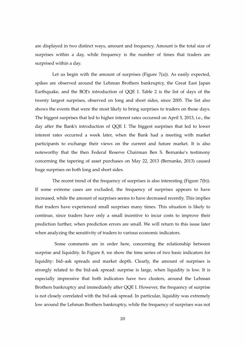
20

are displayed in two distinct ways, amount and frequency. Amount is the total size of

surprises within a day, while frequency is the number of times that traders are

surprised within a day.

Let us begin with the amount of surprises (Figure 7(a)). As easily expected,

spikes are observed around the Lehman Brothers bankruptcy, the Great East Japan

Earthquake, and the BOJ’s introduction of QQE I. Table 2 is the list of days of the

twenty largest surprises, observed on long and short sides, since 2005. The list also

shows the events that were the most likely to bring surprises to traders on those days.

The biggest surprises that led to higher interest rates occurred on April 5, 2013, i.e., the

day after the Bank’s introduction of QQE I. The biggest surprises that led to lower

interest rates occurred a week later, when the Bank had a meeting with market

participants to exchange their views on the current and future market. It is also

noteworthy that the then Federal Reserve Chairman Ben S. Bernanke‘s testimony

concerning the tapering of asset purchases on May 22, 2013 (Bernanke, 2013) caused

huge surprises on both long and short sides.

The recent trend of the frequency of surprises is also interesting (Figure 7(b)).

If some extreme cases are excluded, the frequency of surprises appears to have

increased, while the amount of surprises seems to have decreased recently. This implies

that traders have experienced small surprises many times. This situation is likely to

continue, since traders have only a small incentive to incur costs to improve their

prediction further, when prediction errors are small. We will return to this issue later

when analyzing the sensitivity of traders to various economic indicators.

Some comments are in order here, concerning the relationship between

surprise and liquidity. In Figure 8, we show the time series of two basic indicators for

liquidity: bid–ask spreads and market depth. Clearly, the amount of surprises is

strongly related to the bid-ask spread: surprise is large, when liquidity is low. It is

especially impressive that both indicators have two clusters, around the Lehman

Brothers bankruptcy and immediately after QQE I. However, the frequency of surprise

is not closely correlated with the bid-ask spread. In particular, liquidity was extremely

low around the Lehman Brothers bankruptcy, while the frequency of surprises was not

21

substantially high. This allows us the following interpretation: in the Lehman-Brothers

case, relatively great liquidity shocks hit the market in a distinct way; in the case of

QQE I, however, relatively small liquidity shocks occurred in a continuous way.

3.4. Market reactions to the announcements of the four policy changes

In this paper, we are interested in how monetary policy announcements change, or do

not change, the behavior of market participants. Here we focus on the announcements

of the four policy changes made recently by the BOJ: the QQE I on April 4, 2013; the

QQE II on October 31, 2014; the NIR on January 29, 2016; and the YCC on September 21,

2016. The analysis below indicates the following fact: Having experienced the BOJ

Governor Kuroda’s “bazooka shot”, the QQE I, traders have become rather quick to

learn the BOJ’s intentions embedded in its policy announcements.

Figure 9 shows the intra-day behavior of the fair price, 𝑝𝜏, on the four policy

announcement days. The dots indicate the timing of fair price updates. The fair price

began to swing up and down wildly immediately after the BOJ’s announcement of

QQE I.18 In contrast, after the announcements of NIR and YCC, the adjustment of the

fair price was completed fairly quickly and concentrated around the announcement

time. By seeing the intra-day developments more carefully, we also note that the fair

price was updated more or less around 16:00 on all of the four policy announcement

days. These behaviors of fair prices reflect the importance of the Governor’s press

conference, which is usually held from 15:30 to 16:30 on the policy announcement days,

for the creation of public information.

The case of the announcement of QQE II is counterintuitive at first glance.

Although QQE II were supposed to be very surprising to market participants, fair price

updates were infrequent throughout the day. One of the possible reasons is as follows.

Before the BOJ’s policy announcement, much uncertainty had already pervaded the

market, due to the anticipated announcement by the Government Pension Investment

18 It is also notable that the fair price was updated many times in the morning session on

the day of QQE I.

22

Fund (GPIF) concerning its asset allocation policy. The amplified uncertainty might

have prevented traders from updating fair prices.

Figure 10 shows the marginal value of public information that appeared every

five minutes and its decomposition into expected and unexpected (or surprising) parts.

Following the announcement of QQE I, the appearance of public information was

dispersed over 380 minutes; in contrast, it was concentrated around the time of policy

announcement in the case of NIR and YCC. Similarly, the occurrence of surprises was

dispersed over six hours, following the announcement of QQE I; in contrast, it was

concentrated during the two hours after the policy announcement in the case of NIR

and YCC.19 Almost no surprises were observed in the case of QQE II due to the

aforementioned infrequent fair price updates.

Figure 11 shows the market responses over longer horizons. Figure 11(a)

shows how often the fair price was updated on the day of policy announcement and

over the next five days. In the case of QQE I, the fair price was updated substantially

during the next five days after the policy announcement. In fact, the large swings in the

fair price on the announcement day, shown in Figure 9(a), were followed by much

larger swings on the following days.20 By contrast, more than half of the update was

completed on the day of policy announcement in the case of NIR and YCC. A similar

result is obtained for surprises. As shown in Figures 11(b) and (c), most surprises

occurred during the next five days after the policy announcement in the case of QQE I;

in contrast, they were observed on the very day of policy announcements in the case of

NIR and YCC. Despite nearly zero surprises, in the case of QQE II, behavioral

characteristics of fair price updates and surprises are still close to the case of QQE I.

19 On the day of NIR announcement, big surprises were recorded before the announcement.

This was due to the report by the Nikkei newswire, which broadcast its monetary policy

outlook before the BOJ’s announcement with a headline “the BOJ has discussed setting a

negative interest rate.”

20 The large swings in the fair price after QQE I were consistent with traders’ confusion

noted in footnote 5.

23

3.5. Market behavior just before the announcements of the four policy changes

Here, we examine the market behavior just before the announcements of the four

policy changes. In Figure 12, the complementary cumulative distribution of ask prices

just before the announcement is compared to the corresponding distribution observed

four business days ahead of the announcement (i.e., on the previous day of the

“blackout” before the monetary policy meeting). As in Figure 12(a), the two

distributions coincide mostly with each other in the case of QQE I. As indicated in

Figures 12(b) to (d), however, the distribution on the announcement day is diverted

upward from the corresponding distribution observed four business days ahead of the

announcement in the case of QQE II, NIR, and YCC. An upward diverted

complementary cumulative distribution implies that a price has higher chance of

taking on extreme values, or that a price is distributed with fatter tails. Hence, Figure

12 is the evidence that the market has changed since QQE I and strengthened its

herding behavior on a policy announcement day.

In Figure 13, the bars indicate the sum of �̂�𝑎𝜏 and �̂�𝑏𝜏 observed just before

the announcements. The size of �̂�𝑎𝜏 and �̂�𝑏𝜏 shows how large profit opportunities

traders expect. Traders’ expectations on the announcement day of NIR were smaller

than those on the other three policy announcement days. The introduction of this new

policy was so hard for the majority of traders to expect beforehand. In comparison, on

the announcement day of QQE I, it was no question that new policy measures would

be introduced, whatever they were. As for QQE II and YCC, it is noteworthy that much

uncertainty had already prevailed on their announcement days, that is, on the

announcement day of QQE II due to the anticipated announcement by the GPIF and of

YCC due to the prior notice of publishing Comprehensive Assessment by the BOJ.

There was another source of uncertainty on the three days of QQE I, QQE II,

and YCC. In Figure 13, we show the time gap between the opening of the afternoon

session and the release of the policy announcement.21 Clearly, traders’ expectations are

21 The time of policy announcements release after monetary policy meetings is not

predetermined by the BOJ, in contrast with the Federal Open Market Committee or the

24

correlated with the time gap positively. We pursue this issue further below, using

Figures 14 to 16.

As shown in Figure 14(a), positive correlation has been observed between the

ex ante price mobility of long-side traders and the delays of policy announcements

since Governor Kuroda took his position on March 2013. Here, ex ante price mobility is

measured by 𝑝𝑎𝜏 − 𝑝𝜏−1 on the long side and 𝑝𝜏−1 − 𝑝𝑏𝜏 on the short side, just before

policy announcements (see footnote 9). If policy announcements are delayed, market

participants expect a substantial policy change to be made. This increases traders’

expected marginal value of public information and thus ex ante price mobility. In

contrast, as shown in Figures 14(b) and (c), no such correlation had been observed

during the Shirakawa and Fukui regimes.22 It is also noteworthy that, as shown in

Figure 15(a), no (or even negative) correlation is observed on the short side. That is,

traders’ expectations were so biased toward monetary easing that the risk of monetary

tightening was out of consideration during the sample period. As shown in Figures

15(b) and (c), there is no correlation on the short side during the Shirakawa and Fukui

regimes.

As a related issue, it is interesting to see the effects of live broadcasting of

press conferences on market surprises. On April 8, 2014, the BOJ began on-spot

broadcasting of the Governor’s press conference after the monetary policy meeting. As

shown in Figure 16, on average, surprises measured during and after the press

conference have halved on the long side and have almost been extinguished on the

short side. This proves that quick and direct communication is an effective way to save

market participants from misunderstanding the Bank’s policy announcement.

European Central Bank.

22 Former Governors Shirakawa and Fukui held their positions from April 2008 to March

2013 and from March 2003 to March 2008, respectively. Our sample period, starting from

2005, does not fully cover the Fukui regime.

25

3.6. Market reactions to the release of economic indicators

Not only the central bank’s policy announcements but also economic indicators are

considered to be important public information available in financial markets. Here, we

examine whether market participants’ reaction to economic indicators has changed

since they experienced QQE I. In particular, we focus on traders’ response to the

monthly release of the Indices of Industrial Production (IIP), the Consumer Price Index

(CPI), and the Economy Watchers Survey (EWS).23

Figure 17 shows the size of fair price updates in reaction to the release of the

three economic indicators, traders’ expectations just before the release, and surprises at

the release. The values are averaged over samples prior to the introduction of QQE I

(i.e., April 4, 2013) and later, respectively. As is clearly seen in Figure 17(a), the

reactions to the release of IIP have been downsized by half on average since QQE I. The

size of reactions to the release of CPI has more than halved. Interestingly, the reactions

to the release of the EWS has decreased on the long side but not on the short side,

meaning that traders take the Survey as a useful source to look out for a downturn of

the asset price or for the upturn of the interest rate. On the other hand, as shown in

Figure 17(b), traders’ ex ante marginal value of public information have not decreased

as much as the ex post value. As a result, market surprises have recently become

smaller, as shown in Figure 17(c). As an exceptional case, high interest rate surprises

caused by the release of the EWS have increased slightly.

Several explanations are possible for the downsizing of fair price updates after

QQE I. The first explanation is that the interest rate has little room to move near the

zero lower bound. If this were the case, the upward reaction of fair prices would be

reduced more than the downward reaction. However, no such relationship is observed

in Figure 17(a). Thus, this explanation is not plausible. The second explanation is that

the movements of the economic indicators have declined. However, this explanation is

also implausible when we look at the time series of these indicators. The third and the

most plausible explanation is that the tendency has recently been strengthened that

23 Concerning IIP, we focus on the release of its preliminary results.

26

market participants learn the meaning of each indicator not from their experiences but

from the interpretation by the BOJ. Figure 17(d) shows the size of fair price updates

following policy announcements relative to the size of updates following economic

indicators. Clearly, fair prices are more responsive, both downward and upward, to the

BOJ’s policy announcements than to the release of economic indicators.

The explanation above can be supported by the time taken for the fair price

to update. Figures 18(a) and (b) indicate how many minutes it takes before the fair

price first reacts to the release of economic indicators. The speed at which traders react

to economic indicators, the IIP and the CPI, has become slower since 2011. By contrast,

the speed at which traders respond to the BOJ’s announcements has not slowed.

Figures 18(c) and (d) show how many minutes it takes for the fair price to react to the

release of the statements by the BOJ. Although market participants became temporarily

less sensitive to the Bank’s release of the results of monetary policy meetings after QQE

I, their sensitivity has strengthened again since QQE II. A similar tendency is observed

for traders’ reaction to the BOJ’s announcement of a monthly schedule of government

bond purchases.24 Although they became less sensitive to the release of the asset

purchase schedule after QQE II, this sensitivity has returned to its normal level since

the NIR policy.

In this context, it is also interesting to see the effects on market behavior of

reducing monetary policy meetings. Since 2016, the frequency of the BOJ’s monetary

policy meetings has been reduced from fourteen to eight times a year. And the Bank

ceased to publish the Monthly Report of Recent Economic and Financial Developments,

which was released after the monetary policy meeting. Instead, the issuing of the

Outlook for Economic Activity and Prices, the BOJ’s economic outlook, has increased from

two to four times a year. In addition, the Outlook has richer information than the

Monthly Report. 25 A question is whether the BOJ’s information transmission has

24 After QQE II, the Bank decided to announce the schedule of the outright purchases of

Japanese government bonds for the following month, in principle on the last business day

of every month.

25 While the Monthly Report explains recent economic and financial developments upon

27

weakened or not.

Figure 19(a) shows the reaction of the fair price after the release of the BOJ’s

economic reports (the Outlooks and the Monthly Reports). The reaction to the Outlook is

greater than that to the Monthly Report on average. Interestingly, the total reaction to

the two Outlooks and the twelve Monthly Reports issued in 2015 is almost the same as

the total reaction to the four Outlooks issued in 2016. The new publication scheme

allows the BOJ to send the same amount of information to the market. It is also shown

in Figure 19(b) that the total expected information value of the two Outlooks and the

twelve Monthly Reports is the same as the total expected information value of the four

Outlooks. The amount of information sent by the BOJ, whether realized or expected, has

not been reduced by the reduction of the number of monetary policy meetings and

economic reports.

4. CONCLUSION

In this paper, we present a theoretical model to explain how traders incorporate public

and private information into asset prices by extending Nirei, Takaoka, and Watanabe

(2013) and Kamada and Miura (2014). We also propose an empirical framework that

enables us to fit the model to tick-by-tick data and to identify and quantify surprises in

financial markets, particularly those in the Japanese government bond futures market.

Many shocks caused large surprises in the Japanese bond futures market

during the period from 2005 to 2016, for instance, the Lehman Brothers bankruptcy in

2008, the Great East Japan Earthquake in 2011, the BOJ’s introduction of QQE I in 2013,

and the tapering speech by the then Federal Reserve Chairman Ben S. Bernanke in

2013.

Our empirical analysis also shows that drastic changes occurred in the

sensitivity of bond futures prices to the BOJ’s announcements of new policy measures.

which the Bank bases its monetary policy decisions, the Outlook, in addition to that,

outlines the Bank's views on the future conduct of monetary policy.

28

We examined closely the intra-day developments of market participants’ beliefs. It was

shown that their reactions to the introduction of NIR policy on January 29, 2016 and

YCC on September 21, 2016 were much quicker than those to the introduction of QQE I

on April 4, 2013 and QQE II on October 31, 2014.

Market participants are now so sensitive to the BOJ’s policy actions that the

delay of statement release after monetary policy meetings has a substantial impact on

the price formation in bond futures markets. In this context, the live press conference

broadcast after monetary policy meetings, which was introduced on April 8, 2014, was

effective in reducing surprises in bond futures markets. Similarly, the early

announcement of scheduled dates for government bond purchases, which was

introduced in 2017, is also useful to minimize market surprises.

In contrast, traders’ sensitivity to other economic indicators has weakened. The

impact of IIP, CPI, and EWS on bond futures prices is now smaller than it was before

the introduction of QQE I. Interestingly, the value of information provided by the BOJ’s

economic analysis has not decreased, even though the Bank has reduced the frequency

of monetary policy meetings from fourteen to eight times a year and that of economic

reports from monthly to quarterly.

There remains interesting issues to work on. It is theoretically interesting to

extend the present model by incorporating interaction between the long side and short

side markets, which are now separately treated. It is also interesting empirically to

apply our framework to various financial markets other than Japanese government

bond futures markets. The same policy announcements by the BOJ might have a

different impact on the stock market, the foreign exchange market, and so on. We hope

to address these interesting issues elsewhere in the near future.

29

APPENDIX. PROOF OF THE EXISTENCE OF MARKET EQUILIBRIUM

Lemma 1. �̅�𝜏(𝑘) is monotonically decreasing in 𝑘 when 𝑛𝑎 is sufficiently large.

𝑥𝜏( ) is monotonically increasing in when 𝑛𝑏 is sufficiently large.

Transforming equation (9) yields

𝑎𝜏(𝑘) (�̅�𝜏(𝑘)) −

(�̅�𝜏(𝑘)) −1𝛿(�̅�𝜏(𝑘)), (A1)

where

𝑎𝜏(𝑘) ≡

(1 − �̂�𝑎𝜏) − �̂�𝑎𝜏1𝜃𝜏−1

𝑝𝐻 − 𝑝𝑎𝜏(𝑘)𝑝𝑎𝜏(𝑘) − 𝑝𝐿

(1 − �̂�𝑎𝜏)1𝜃𝜏−1

𝑝𝐻 − 𝑝𝑎𝜏(𝑘)𝑝𝑎𝜏(𝑘) − 𝑝𝐿

− �̂�𝑎𝜏

(A2)

Taking the log differences of both sides of equation (A1) yields

(�̅�𝜏(𝑘))

(�̅�𝜏(𝑘))

𝑎𝜏(𝑘 1)

𝑎𝜏(𝑘)

(𝑛𝑎 − 𝑘 − 1) (�̅�𝜏(𝑘 1))

(�̅�𝜏(𝑘)) 𝑘

(�̅�𝜏(𝑘 1))

(�̅�𝜏(𝑘))

𝛿(�̅�𝜏(𝑘 1))

𝛿(�̅�𝜏(𝑘)) (A3)

The first term on the left-hand side is positive since (𝑥) > (𝑥) It is clear from

equation (16) that as 𝑛𝑎 increases, the difference between (𝑘 1)/𝑛𝑎 and 𝑘/𝑛𝑎

converges to zero, and so does the difference between 𝑝𝑎𝜏(𝑘 1) and 𝑝𝑎𝜏(𝑘). Thus,

the difference between 𝑎𝜏(𝑘 1) and 𝑎𝜏(𝑘) converges to zero, and so does the

second term on the left-hand side. This implies that the left-hand side of equation (A3)

is positive when 𝑛𝑎 is sufficiently large. Since (𝑥) , (𝑥) , and 𝛿(𝑥) are all

decreasing in 𝑥, the right-hand side is positive only if �̅�𝜏(𝑘) > �̅�𝜏(𝑘 1). This shows

that �̅�𝜏(𝑘) is decreasing in 𝑘. Similarly, we can show that 𝑥𝜏( ) is increasing in

when 𝑛𝑏 is sufficiently large.

Proposition 1. There exists a 𝑘∗ that satisfies 𝐷𝑎𝜏(𝑘∗) 𝑘∗ when 𝑛𝑎 is sufficiently

30

large. Moreover, there exists an ∗ that satisfies 𝑏𝜏( ∗) ∗ when 𝑛𝑏 is

sufficiently large.

We know from Lemma 1 that �̅�𝜏(𝑘) is monotonically decreasing in 𝑘. Thus, 𝐷𝑎𝜏 is a

monotonic mapping. Therefore, following Nirei, Takaoka, and Watanabe (2013), we can

show the existence of equilibrium 𝑘∗ using Tarski’s fixed-point theorem for a discrete

monotonic mapping. The existence of equilibrium ∗ can be proved in a similar

manner.

REFERENCES

Andersson, Magnus (2010), “Using Intraday Data to Gauge Financial Market

Responses to Federal Reserve and ECB Monetary Policy Decisions,” International

Journal of Central Banking, June 2010, pp. 117-146.

Banerjee, Abhijit V. (1992), “A Simple Model of Herd Behavior,” Quarterly Journal of

Economics, Vol. 107, No. 3, pp. 797-817.

Bank of Japan (2013), “Introduction of the ‘Quantitative and Qualitative Monetary

Easing’,” April 4, 2013,

http://www.boj.or.jp/en/announcements/release_2013/k130404a.pdf.

-------------------- (2014), “Expansion of the Quantitative and Qualitative Monetary

Easing,” October 31, 2014,

http://www.boj.or.jp/en/announcements/release_2014/k141031a.pdf.

-------------------- (2016a), “Introduction of ‘Quantitative and Qualitative Monetary

Easing with a Negative Interest Rate’,” January 29, 2016,

http://www.boj.or.jp/en/announcements/release_2016/k160129a.pdf.

-------------------- (2016b), “New Framework for Strengthening Monetary Easing:

‘Quantitative and Qualitative Monetary Easing with Yield Curve Control’,”

September 21, 2016,

http://www.boj.or.jp/en/announcements/release_2016/k160921a.pdf.

-------------------- (2017), “Liquidity Indicators in the JGB Markets,”December 27, 2017,

31

http://www.boj.or.jp/en/paym/bond/ryudo.pdf.

Bernanke, Ben S. (2013), “Statement by Ben S. Bernanke, Chairman of the Board of

Governors of the Federal Reserve System before the Joint Economic Committee,”

May 22, 2013,

http://www.federalreserve.gov/newsevents/testimony/files/bernanke20130522a.p

df.

Blinder, Alan S.; Michael Ehrmann; Marcel Fratzscher; Jakob De Haan; and David-Jan

Jansen (2008), “Central Bank Communication and Monetary Policy: A Survey of

Theory and Evidence,” Journal of Economic Literature, Vol. 46, No. 4, pp. 910-945.

Cochrane, John H., and Monika Piazzesi (2002), “The Fed and Interest Rates -- A

High-Frequency Identification,” American Economic Review, Vol. 92, No. 2, pp.

90-95.

Cutler, David M.; James M. Poterba; and Lawrence H. Summers (1989), “What Moves

Stock Prices?” Journal of Portfolio Management, Vol. 15, No. 3, pp. 4-12.

Fleming, Michael J., and Monika Piazzesi (2005), “Monetary Policy Tick-by-Tick,”

http://www.bankofcanada.ca/wp-content/uploads/2010/08/flemming.pdf.

--------------------, and Eli M. Remolona (1997), “What Moves the Bond Market?” FRBNY

Economic Policy Review, December 1997, pp. 31-50.

--------------------, and -------------------- (1999), “Price Formation and Liquidity in the U.S.

Treasury Market: The Response to Public Information,” Journal of Finance, Vol.

LIV, No. 5, pp. 1901-1915.

Gabaix, Xavier; Parameswaran Gopikrishnan; Vasiliki Plerou; and H. Eugene Stanley

(2006), “Institutional Investors and Stock Market Volatility,” Quarterly Journal of

Economics, Vol. 121, No. 2, pp. 461-504.

Honda, Yuzo, and Yoshihiro Kuroki (2006), “Financial and Capital Markets' Responses

to Changes in the Central Bank's Target Interest Rate: The Case of Japan,”

Economic Journal, Vol. 116, No. 513, pp. 812–842.

Kamada, Koichiro (2014), “Central Bank Communication and the Management of

32

Market Confidence: Two Episodes in 2013 in the U.S. and Japan,” Bank of Japan

Research Laboratory Series, No. 14-E-1.

--------------------, and Ko Miura (2014), “Confidence Erosion and Herding Behavior in

Bond Markets: An Essay on Central Bank Communication Strategy,” Bank of

Japan Working Paper Series, No. 14-E-6.

Kuttner, Kenneth N. (2001), “Monetary Policy Surprises and Interest Rates: Evidence

from the Fed Funds Futures Market,” Journal of Monetary Economics, Vol. 47, No. 3,

pp. 523-544.

Lillo, Fabrizio; J. Doyne Farmer; and Rosario N. Mantegna (2003), “Master Curve for

Price-Impact Function,” Nature, Vol. 421, pp. 129-130.

Morris, Stephen, and Hyun Song Shin (2002), “Social Value of Public Information,”

American Economic Review, Vol. 92, No. 5, pp. 1521-1534.

Nakamura, Emi, and Jón Steinsson (2018), “High Frequency Identification of Monetary

Non-Neutrality: The Information Effect,” NBER Working Paper No. 19260.

Nirei, Makoto; Koichiro Takaoka; and Tsutomu Watanabe (2013), “Beauty Contests and

Fat Tails in Financial Markets,” http://ssrn.com/abstract=2362341.

Rigobon, Roberto, and Brian Sack (2004), “The Impact of Monetary Policy on Asset

Prices,” Journal of Monetary Economics, Vol. 51, No. 8, pp. 1553-1575.

33

Table 1. Definition of Surprises

(a) Identification

Surprise No surprise

Price base 𝑝𝜏 < 𝑝𝑏𝜏 or 𝑝𝑎𝜏 < 𝑝𝜏 𝑝𝑏𝜏 𝑝𝜏 𝑝𝑎𝜏

Information value base 𝜂𝜏 < �̂�𝑎𝜏 or �̂�𝑏𝜏 < 𝜂𝜏 �̂�𝑎𝜏 𝜂𝜏 �̂�𝑏𝜏

(b) Quantification

Price base ( 𝑝𝜏 − 𝑝𝑎𝜏)

or ( 𝑝𝜏 − 𝑝𝑏𝜏)−

Information value base ( 𝜂𝜏 − �̂�𝑎𝜏)− or ( 𝜂𝜏 − �̂�𝑏𝜏)

34

Table 2. The Twenty Largest Surprises

(a) Low interest rate surprises

Note: After surprises are quantified as ( 𝑝𝜏 − 𝑝𝑎𝜏)

, each day is ranked by the amount

of surprises within the day.

Ranking Date Event Surprise

1 2013/4/11The BOJ had a meeting with market participants to exchange their

views on the current and future market （4/11）0.01326

2 2008/9/16 Bankruptcy of Lehman Brothers （9/15） 0.01310

3 2013/4/5 Introduction of QQE I by the BOJ （4/4） 0.01073

4 2008/9/10 Calendar rollover with large negative spreads （9/10） 0.00945

5 2013/5/23 Tapering speech by Federal Reserve Chairman Bernanke （5/22） 0.00781

6 2008/10/29Mounting expectation of interest rate cuts at the forthcoming BOJ

policy meeting （10/29）0.00778

7 2013/4/12Governer Kuroda made a speech in Tokyo for the first time after

the introduction of QQE I （4/12）0.00639

8 2007/11/2Governer Fukui was summoned to the House of Representatives,

Financial Monetary Committee （11/2）0.00567

9 2013/5/15The BOJ offered 2.8 trillion yen under the funds-supplying

operation （5/15）0.00543

10 2007/12/12 The FOMC announced interest rate cut by 25bps （12/11） 0.00543

11 2007/11/27Decline in U.S. interest rates due mainly to the subprime

mortgage problem （11/26）0.00453

12 2011/3/14 The Great East Japan Earthquake （3/11） 0.00394

13 2013/6/25Strong demand for JGBs in the auction for enhanced-liquidity.

The bid-to-cover ratio was 5.95 （6/25）0.00394

14 2006/9/22 −−− 0.00394

15 2013/6/13Member of the BOJ Policy Board Shirai made a speech in

Asahikawa （6/13）0.00379

16 2013/5/22 The BOJ maintained the current policy （5/22） 0.00374

17 2007/8/29 −−− 0.00369

18 2008/5/16 −−− 0.00363

19 2013/5/17 The BOJ offered outright purchase of 1.3 trillion yen JGBs （5/17） 0.00358

20 2009/3/19 The FOMC announced the starting of treasury purchases （3/18） 0.00352

c.f.

60 2016/1/29 Introduction of NIR by the BOJ (1/29) 0.00200

71 2016/9/21 Introduction of YCC by the BOJ (9/21) 0.00178

35

(b) High interest rate surprises

Note: After surprises are quantified as ( 𝑝𝜏 − 𝑝𝑏𝜏)−

, each day is ranked by the amount

of surprises within the day.

Ranking Date Event Surprise

1 2013/4/5 Introduction of QQE I by the BOJ （4/4） -0.01537

2 2006/6/9 Calendar rollover （6/9） -0.01203

3 2013/5/15It was reported that the Cabinet Ministers implied that a rise in

interest rates was not an issue （5/14）-0.01178

4 2013/5/23 Tapering speech by Federal Reserve Chairman Bernanke （5/22） -0.00989

5 2010/12/9 Calendar rollover （12/9） -0.00874

6 2006/3/9 Termination of QE by the BOJ （3/9） -0.00862

7 2007/3/9 Calendar rollover （3/9） -0.00779

8 2008/6/11 Calendar rollover （6/11） -0.00771

9 2008/5/23 −−− -0.00764

10 2013/4/8 A circuit breaker was triggered in the JGB futures market （4/8） -0.00739

11 2008/10/9The BOJ did not coordinate with accomodative interest rate cuts

by six central banks in the U.S. and Europe （10/8）-0.00562

12 2005/3/10 Calendar rollover （3/10） -0.00544

13 2013/5/24 Tapering speech by Federal Reserve Chairman Bernanke （5/22） -0.00513

14 2013/4/12Governer Kuroda made a speech in Tokyo for the first time after

the introduction of QQE I （4/12）-0.00500

15 2013/4/11The BOJ had a meeting with market participants to exchange their

views on the current and future market （4/11）-0.00492

16 2008/6/13 The BOJ's monetary policy meeting （6/13） -0.00475

17 2013/12/11 Calendar rollover （12/11） -0.00443

18 2008/11/14The Ministry of Finance held a meeting of JGB Market Special

Participants （11/14）-0.00384

19 2010/12/15The BOJ released the results of December 2010 Tankan survey

（12/15）-0.00367

20 2007/6/13 −−− -0.00366

36

Figure 1. Demand Function of Long-Side Informed Traders

Figure 2. Fat-Tail Distribution of Asset Prices

Note: Private information is generated from 𝐹𝐻. The simulation is iterated 25,000 times

each for long and short sides.

-6

-4

-2

0

2

4

6

8

3 2 1 0 1 2 3

Long side

Short side

Exponential

Normal

ln (relative frequency)

Percent change

in ask prices

Percent change

in bid prices

𝑥𝜏(𝑘)

1 2 3 𝑘 0

𝑥𝑖𝜏

𝑥2𝜏

𝑥1𝜏

(a) Investment decision-making based

on private information

(b) Shape of the demand function

Demand

𝑝𝑎𝜏(2)

𝑝𝑎𝜏(1)

𝑝𝑎𝜏(4)

𝑝𝑎𝜏(𝑘)

1 2 3 0

𝑝𝑎𝜏(3)

37

Figure 3. Comparative Statics of the Asset Price Distribution

Note: Private information is generated from 𝐹𝐻. The simulation is iterated 25,000 times

each for long and short sides.

(a) Effects of likelihood ratios

(b) Effects of traders’ expected marginal

value of public information

(c) Effects of accuracy of private

information (mean difference)

(d) Effects of accuracy of private

information (standard deviation)

(e) Effects of market liquidity

-6

-4

-2

0

2

4

6

8

3 2 1 0 1 2 3

θ0 = 0.1

θ = 1

θ = 10

ln (relative frequency)

θτ-1 = 0.1

θτ-1= 1

θτ-1= 10

Percent change

in ask prices

Percent change

in bid prices

-6

-4

-2

0

2

4

6

8

3 2 1 0 1 2 3

q = 0.6

q = 0.8

ln (relative frequency)

Percent change

in ask prices

Percent change

in bid prices

-6

-4

-2

0

2

4

6

8

3 2 1 0 1 2 3

ln (relative frequency)

Percent change

in ask prices

Percent change

in bid prices

μH - μL = 1

μH - μL = 2

-6

-4

-2

0

2

4

6

8

3 2 1 0 1 2 3

σ = 400

σ = 200

ln (relative frequency)

Percent change

in ask prices

Percent change

in bid prices

-6

-4

-2

0

2

4

6

8

3 2 1 0 1 2 3

λ = 0.4

λ = 0.8

λ = 1

ln (relative frequency)

Percent change

in ask prices

Percent change

in bid prices

38

Figure 4. Fitting the Model to Tick-by-Tick Data

(a) Surprises identified (b) No surprises identified

Figure 5. Fair Prices and Traders’ Beliefs

(a) Estimated fair prices (b) Traders’ beliefs on financial states

Notes: 1. Four vertical lines in each chart correspond to QQE I on April 4, 2013, QQE II on

October 31, 2014, NIR on January 29, 2016, and YCC on September 21, 2016,

respectively. This also applies to the following figures.

2. Figures are averaged on each day.

13,000

13,500

14,000

14,500

15,000

15,500

05 06 07 08 09 10 11 12 13 14 15 16

JPY cents

↑Lower interest rates

↓Higher interest rates

CY

QQE I QQE II NIR YCC

0.0

0.5

1.0

1.5

2.0

2.5

3.0

05 06 07 08 09 10 11 12 13 14 15 16

↑Higher interest rates

↓Lower interest rates

CY

QQE I QQE II NIR YCC

39

Figure 6. Realized and Expected Marginal Value of Public Information

Notes: 1. The realized marginal value of public information is depicted as the range

between the maximum and the minimum value of 𝜂𝜏 within each day.

2. The expected marginal value of public information is depicted as the range

between the maximum value of �̂�𝑏𝜏 and the minimum value of �̂�𝑎𝜏 within each

day.

(a) Realized marginal value of public

information

(b) Expected marginal value of public

information

0.85

0.90

0.95

1.00

1.05

1.10

1.15

05 06 07 08 09 10 11 12 13 14 15 16

↑Information indicating a high-interest-rate state↓Information indicating a low-interest-rate state

CY

QQE I QQE II NIR YCC

0.85

0.90

0.95

1.00

1.05

1.10

1.15

05 06 07 08 09 10 11 12 13 14 15 16

↑Information indicating a high-interest-rate state↓Information indicating a low-interest-rate state

CY

QQE I QQE II NIR YCC

40

Figure 7. Surprises

(a) Amount of surprises

(a-1) Low interest rate surprises (a-2) High interest rate surprises

(b) Frequency of surprises

(b-1) Low interest rate surprises (b-2) High interest rate surprises

Notes: 1. Amount of surprises is the total size of surprises within a day. Frequency of

surprises is the number of times that traders are surprised within a day.

2. For amount, low and high interest rate surprises are quantified as ( 𝑝𝜏 − 𝑝𝑎𝜏)

and ( 𝑝𝜏 − 𝑝𝑏𝜏)−

, respectively.

0

5

10

15

20

25

30

35

40

45

50

55

05 06 07 08 09 10 11 12 13 14 15 16

times

CY

QQE I QQE II NIR YCC

0

5

10

15

20

25

30

35

40

45

50

55

05 06 07 08 09 10 11 12 13 14 15 16CY

times QQE I QQE II NIR YCC

-0.016

-0.014

-0.012

-0.010

-0.008

-0.006

-0.004

-0.002

0.000

05 06 07 08 09 10 11 12 13 14 15 16CY

QQE I QQE II NIR YCC

0.000

0.002

0.004

0.006

0.008

0.010

0.012

0.014

0.016

05 06 07 08 09 10 11 12 13 14 15 16CY

QQE I QQE II NIR YCC

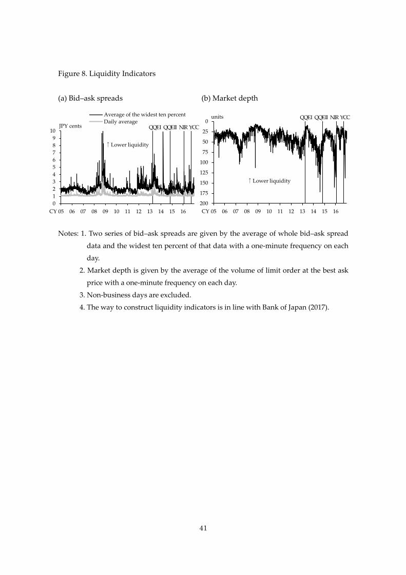
41

Figure 8. Liquidity Indicators

(a) Bid–ask spreads (b) Market depth

Notes: 1. Two series of bid–ask spreads are given by the average of whole bid–ask spread

data and the widest ten percent of that data with a one-minute frequency on each

day.

2. Market depth is given by the average of the volume of limit order at the best ask

price with a one-minute frequency on each day.

3. Non-business days are excluded.

4. The way to construct liquidity indicators is in line with Bank of Japan (2017).

0

25

50

75

100

125

150

175

200

05 06 07 08 09 10 11 12 13 14 15 16CY

units

↑Lower liquidity

QQE I QQE II NIR YCC

0

1

2

3

4

5

6

7

8

9

10

05 06 07 08 09 10 11 12 13 14 15 16

Average of the widest ten percent

Daily average

CY

JPY cents

↑Lower liquidity

QQE I QQE II NIR YCC

42

Figure 9. Intra-Day Developments of Fair Prices

(a) QQE I (April 4, 2013) (b) QQE II (October 31, 2014)

(c) NIR (January 29, 2016) (d) YCC (September 21, 2016)

Note: Vertical lines correspond to announcement times.

14,530

14,550

14,570

14,590

14,610

14,630

14,650

0:00 4:00 8:00 12:00 16:00 20:00

JPY cents

14,640

14,645

14,650

14,655

14,660

14,665

14,670

14,675

14,680

0:00 4:00 8:00 12:00 16:00 20:00

JPY cents

14,940

14,960

14,980

15,000

15,020

15,040

15,060

15,080

15,100

0:00 4:00 8:00 12:00 16:00 20:00

JPY cents

15,100

15,120

15,140

15,160

15,180

15,200

15,220

0:00 4:00 8:00 12:00 16:00 20:00

JPY cents

43

-0.015

-0.010

-0.005

0.000

0.005

0.010

0.015

0.020

-300

~-29

5

-250

~-24

5

-200

~-19

5

-150

~-14

5

-100

~-95

-50~

-45

0~5

50~5

5

100~

105

150~

155

200~

205

250~

255

300~

305

350~

355

400~

405

450~

455

500~

505

Unexpected (long side)

Unexpected (short side)

Expected

minutes

-0.015

-0.010

-0.005

0.000

0.005

0.010

0.015

0.020

-300

~-29

5

-250

~-24

5

-200

~-19

5

-150

~-14

5

-100

~-95

-50~

-45

0~5

50~5

5

100~

105

150~

155

200~

205

250~

255

300~

305

350~

355

400~

405

450~

455

500~

505

Unexpected (long side)

Unexpected (short side)

Expected

minutes

-0.015

-0.010

-0.005

0.000

0.005

0.010

0.015

0.020

-300

~-29

5

-250

~-24

5

-200

~-19

5

-150

~-14

5

-100

~-95

-50~

-45

0~5

50~5

5

100~

105

150~

155

200~

205

250~

255

300~

305

350~

355

400~

405

450~

455

500~

505

Unexpected (long side)

Unexpected (short side)

Expected

minutes

-0.015

-0.010

-0.005

0.000

0.005

0.010

0.015

0.020

-300

~-29

5

-250

~-24

5

-200

~-19

5

-150

~-14

5

-100

~-95

-50~

-45

0~5

50~5

5

100~

105

150~

155

200~

205

250~

255

300~

305

350~

355

400~

405

450~

455

500~

505

Unexpected (long side)

Unexpected (short side)

Expected

minutes

Figure 10. Expected and Unexpected Marginal Value of Public Information

(a) QQE I (April 4, 2013) (b) QQE II (October 31, 2014)

(c) NIR (January 29, 2016) (d) YCC (September 21, 2016)

Notes: 1. Unexpected components are surprises quantified as ( 𝜂𝜏 − �̂�𝑎𝜏)− or

( 𝜂𝜏 − �̂�𝑏𝜏) . Expected components are derived by subtracting unexpected

components from log realized marginal value of public information, 𝜂𝜏.

2. Vertical lines correspond to announcement times adjusted to zero. Figures are

summed at the timing of fair price updates at intervals of five minutes.

44

Figure 11. Market Responses Observed over a Longer Horizon

(a) Frequency of fair price updates

(b) Low interest rate surprises

(c) High interest rate surprises

Notes: 1. Frequency of fair price updates is weighted by the absolute realized marginal

value of public information, 𝜂𝜏 . Low and high interest rate surprises are

quantified as −( 𝜂𝜏 − �̂�𝑎𝜏)− and ( 𝜂𝜏 − �̂�𝑏𝜏)

, respectively.

2. Figures on the announcement day are summed up at intervals between the

policy announcement and the closing of the subsequent night session.

0.0

0.2

0.4

0.6

0.8

1.0

0.0

0.2

0.4

0.6

0.8

1.0

1.2

QQE I QQE II NIR YCC

On the announcement day and the next five days <B>On the announcement day <A>Ratio of <A> to <B> (right axis)

0.0

0.2

0.4

0.6

0.8

1.0

0.00

0.02

0.04

0.06

0.08

0.10

0.12

0.14

0.16

0.18

QQE I QQE II NIR YCC

On the announcement day and the next five days <B>On the announcement day <A>Ratio of <A> to <B> (right axis)

0.0

0.2

0.4

0.6

0.8

1.0

0.00

0.05

0.10

0.15

0.20

0.25

0.30

QQE I QQE II NIR YCC

On the announcement day and the next five days <B>On the announcement day <A>Ratio of <A> to <B> (right axis)

45

Figure 12. Herding Behavior Reinforced before Policy Announcements

(a) QQE I (April 4, 2013) (b) QQE II (October 31, 2014)

(c) NIR (January 29, 2016) (d) YCC (September 21, 2016)

Note: Normal distributions are depicted as a reference, where mean is zero and standard

deviation is equal to the median of the distribution observed four business days

ahead of policy announcements.

0.0

0.2

0.4

0.6

0.8

1.0

0.00 0.01 0.02 0.03 0.04 0.05

Just before the policy

announcement on April 4, 2013The same time period on March

29, 2013Normal

Complementary cumulative distribution

Percent change in ask prices

0.0

0.2

0.4

0.6

0.8

1.0

0.00 0.01 0.02 0.03 0.04 0.05

Just before the policy

announcement on January 29,

2016The same time period on

January 25, 2016

Normal

Complementary cumulative distribution

Percent change in ask prices

0.0

0.2

0.4

0.6

0.8

1.0

0.00 0.01 0.02 0.03 0.04 0.05

Just before the policy

announcement on October 31, 2014The same time period on October

27, 2014Normal

Complementary cumulative distribution

Percent change in ask prices

0.0

0.2

0.4

0.6

0.8

1.0

0.00 0.01 0.02 0.03 0.04 0.05

Just before the policy

announcement on September 21,

2016The same time period on

September 14, 2016

Normal

Complementary cumulative distribution

Percent change in ask prices

46

Figure 13. Uncertainty Enlarged by Policy Announcement Delays

Notes: 1. Long-side and short-side uncertainty is given by the ex ante absolute expected

marginal values of public information, i.e., �̂�𝑎𝜏 and �̂�𝑏𝜏 , respectively.

2. Time gap is the gap between the opening of the afternoon session (i.e., 12:30) and

the release of the policy announcement.

0

10

20

30

40

50

60

70

80

0.000

0.001

0.002

0.003

0.004

QQE I QQE II NIR YCC

Short-side uncertainty just before the policy announcement

Long-side uncertainty just before the policy announcement

Time gap (right axis)

minutes

47

Figure 14. Market Reaction to Policy Announcement Delays on the Long Side

(a) Kuroda regime

(b) Shirakawa regime

(c) Fukui regime

Notes: 1. Dots correspond to policy announcements released before 15:00. The

announcement on October 31, 2008 is excluded because of extraordinarily high

price mobility.

2. Vertical gray lines correspond to average time gap and divide samples under

each regime. Red circles and blue (green) squares represent policy announcements

released earlier (later) than the average, respectively.

y = 0.0432x + 2.8614

R² = 0.3526

y = -0.0229x + 2.0112

R² = 0.0235

0

2

4

6

8

10

12

14

-60 -40 -20 0 20 40 60 80 100 120 140Time gap (minutes)

Ex ante price

mobility (JPY cents)

QQE I

QQE II

NIR

YCC

y = 0.0038x + 4.9195

R² = 0.0007

y = 0.0107x + 3.9251

R² = 0.0036

0

5

10

15

20

25

30

-60 -40 -20 0 20 40 60 80 100 120 140Time gap (minutes)

Ex ante price

mobility (JPY cents)

y = 0.0131x + 3.7174

R² = 0.0341y = 0.0168x + 4.4179

R² = 0.0176

0

2

4

6

8

10

12

-60 -40 -20 0 20 40 60 80 100 120 140Time gap (minutes)

Ex ante price

mobility (JPY cents)

48

Figure 15. Market Reaction to Policy Announcement Delays on the Short Side

(a) Kuroda regime

(b) Shirakawa regime

(c) Fukui regime

Notes: 1. Dots correspond to policy announcements released before 15:00. The

announcement on October 31, 2008 is excluded because of extraordinarily high

price mobility.

2. Vertical gray lines correspond to average time gap and divide samples under

each regime. Red circles and blue (green) squares represent policy announcements

released earlier (later) than the average, respectively.

y = -0.0434x + 6.3103

R² = 0.1934

y = -0.023x + 4.6634

R² = 0.0061

0

2

4

6

8

10

12

14

-60 -40 -20 0 20 40 60 80 100 120 140

QQE I

QQE IINIR

YCC

Time gap (minutes)

Ex ante price

mobility (JPY cents)

y = 0.0038x + 4.9533

R² = 0.0055

y = -0.0137x + 3.7371

R² = 0.0119

0

5

10

15

20

25

30

-60 -40 -20 0 20 40 60 80 100 120 140Time gap (minutes)

Ex ante price

mobility (JPY cents)

y = 0.0023x + 4.3552

R² = 0.0024

y = -0.004x + 3.5893

R² = 0.0013

0

2

4

6

8

10

12

-60 -40 -20 0 20 40 60 80 100 120 140Time gap (minutes)

Ex ante price

mobility (JPY cents)

49

Figure 16. Effects of Broadcasting the Governor’s Press Conference

(a) Low interest rates surprises (b) High interest rates surprises

Notes: 1. Surprises are quantified in the same way as in Figure 7 and summed at the

interval between 15:30 and 17:30 on the policy announcement days. While the

press conference is usually held from 15:30 to 16:30, the interval between 16:30 to

17:30 is included to capture ex post responses of traders. If the press conference

starts after 15:30, the interval for summing surprises is moved accordingly. If the

press conference starts after the closing of the night session, the interval for

summing surprises is an hour after the opening of the morning session on the

next day.

2. Average is taken over samples with non-zero surprises prior to April 8, 2014 and

later, respectively.

0.E+00

1.E-04

2.E-04

3.E-04

4.E-04

5.E-04

05 06 07 08 09 10 11 12 13 14 15 16

Average surprise Surprise

Live broadcasting

since April 8, 2014

CY

QQE I QQE II NIR YCC-3.E-03

-3.E-03

-2.E-03

-2.E-03

-1.E-03

-5.E-04

0.E+00

05 06 07 08 09 10 11 12 13 14 15 16

Average surprise Surprise

CY

Live broadcasting

since April 8, 2014

QQE I QQE II NIR YCC

50

Figure 17. Fair Price Updates, Traders’ Expectations, and Surprises at the Release of

Economic Indicators: Comparisons before and after QQE I

(a) Fair price updates (b) Traders’ expectations

(c) Surprises

Notes: 1. Ex post updates of the fair price are given by log differences between the fair price

just before the release of economic indicators and the last fair price before the

closing of the subsequent night session. Positive and negative fair price updates

correspond to those on the long and short sides, respectively.

2. Ex ante price mobility is given by 𝑝𝑎𝜏− 𝑝𝜏−1 for the long side and 𝑝𝑏𝜏 − 𝑝𝜏−1

for the short side just before the release of economic indicators.

3. Surprises are quantified in the same way as in Figure 7 and summed at the

intervals between the release of economic indicators and the closing of the

subsequent night session.

4. In the case where the indicators’ release day coincides with the policy

announcement day, fair price updates and surprises are replaced with zero.

(d) Fair price updates following policy announcements relative to those following the release of economic indicators

-2.E-03

-1.E-03

0.E+00

1.E-03

2.E-03

Before

QQE I

After

QQE I

Before

QQE I

After

QQE I

Before

QQE I

After

QQE I

Ex post update of the fair price (long side)Ex post update of the fair price (short side)

EWSIIP CPI

-3

-2

-1

0

1

2

3

Before

QQE I

After

QQE I

Before

QQE I

After

QQE I

Before

QQE I

After

QQE I

Ex post update of the fair price (long side)Ex post update of the fair price (short side)

EWSIIP CPI

-8.E-04

-6.E-04

-4.E-04

-2.E-04

0.E+00

2.E-04

4.E-04

6.E-04

8.E-04

Before

QQE I

After

QQE I

Before

QQE I

After

QQE I

Before

QQE I

After

QQE I

Low interest rate surpriseHigh interest rate surprise

EWSIIP CPI

-8

-6

-4

-2

0

2

4

6

8

Before

QQE I

After

QQE I

Before

QQE I

After

QQE I

Before

QQE I

After

QQE I

Ex ante price mobility (long side)Ex ante price mobility (short side)

EWSIIP CPI

51

Figure 18. Time to the First Responses to Economic News and Statements by the BOJ

(a) IIP (b) CPI

(c) Policy announcements (d) Operation schedule

Note: The time gap is between the news release and the first update of the fair price after

the release. If the release of a policy announcement comes after the closing of the

night session, it is excluded from samples.

0

100

200

300

400

500

600

05 06 07 08 09 10 11 12 13 14 15 16CY

minutes QQE I QQE II NIR YCC

0

100

200

300

400

500

600

700

05 06 07 08 09 10 11 12 13 14 15 16

minutes

CY

QQE I QQE II NIR YCC

0

100

200

300

400

500

Ap

r-13

Oct

-13

Ap

r-14

Oct

-14

Ap

r-15

Oct

-15

Ap

r-16

Oct

-16

minutes QQE II NIR YCC

0

300

600

900

1,200

1,500

05 06 07 08 09 10 11 12 13 14 15 16CY

minutes QQE I QQE II NIR YCC

52

Figure 19. Total Information Value of the BOJ’s Economic Analysis: Fair Price Updates

and Traders’ Expectations for the Release of Economic Reports

(a) Fair price updates

(b) Traders’ expectations

Notes: 1. Ex post updates of the fair price are on the absolute value basis. Ex ante price

mobility is the total mobility on both long and short sides. Otherwise,

computations for the release of economic reports are the same as in Figure 16

for the release of economic indicators.

2. Of the two Aprils and Octobers of 2015 on each graph, the former and the

latter correspond to the release of the Monthly Report and the Outlook,

respectively.

0.000

0.004

0.008

0.012

0.016

0

0.001

0.002

0.003

0.004

0.005

0.006

0.007

Jan

.

Feb

.

Mar

.

Ap

r.

Ap

r.

May

Jun

e

July

Au

g.

Sep

.

Oct

.

Oct

.

No

v.

Dec

.

Jan

.

Ap

r.

July

No

v.

Ex post update of the fair price (2016 total, right axis)

Ex post update of the fair price (2015 total, right axis)

Ex post update of the fair price (2016)

Ex post update of the fair price (2015)

2015 2016

New publication

scheme

0

5

10

15

20

Jan

.

Feb

.

Mar

.

Ap

r.

Ap

r.

May

Jun

e

July

Au

g.

Sep

.

Oct

.

Oct

.

No

v.

Dec

.

Jan

.

Ap

r.

July

No

v.

Ex ante price mobility (2016 average)

Ex ante price mobility (2015 average)

Ex ante price mobility (2016)

Ex ante price mobility (2015) New publication

schemeJPY cents

2015 2016