Embed Size (px)
Citation preview

Kognitio SQL Guide
Version 7.2.1 July 2012
Notices This document contains proprietary information that should not be reproduced in whole or in part, nor released to third parties nor used for purposes other than those for which it has been expressly provided without the prior written agreement of Kognitio.
Kognitio tries to ensure that the information in this document is correct and fairly stated, but does not accept liability for any error or omission.
Standards Compliance The Kognitio SQL implementation is fully compliant with the ANSI '89 standard.
Kognitio SQL Guide, July 2012 Kognitio Technology Centre © Kognitio Limited, 2002-2012 3A Waterside Park, Cookham Road BRACKNELL, Berks, RG12 1RB United Kingdom
Preface
Kognitio SQL Guide iii
About this Manual
This manual is part of a series that describes how Kognitio can enhance the productivity of your interactive database applications.
The manual assumes that the reader is familiar with relational concepts and SQL. Many excellent SQL reference books already exist and so this manual does not attempt to explain all the details of the language; choosing instead to focus on the data types, statements, functions and operators supported by Kognitio. This manual is however essential for anyone wishing to obtain the maximum benefit from using Kognitio as it is the only source of information on some of the Kognitio extensions to SQL.
The manual also contains a script (Appendix A) which illustrates how many of the concepts can be used together to create a dataset and analyze it. Appendix B provides information about creating SQL scripts that can be run via wxsubmit. Appendix C lists all the SQL reserved words.

Kognitio SQL Guide v
Contents
About this Manual ................................................................................ iii
Contents .............................................................................................. v
1 Data Definition ................................................................................................. 1
1.1 Data Types ................................................................................................ 1
String Data Types ................................................................................ 1
Approximate Numeric Types ............................................................... 3
Exact Numeric Types .......................................................................... 4
Intervals, Dates and Times .................................................................. 5
DATE-TIMES ....................................................................................... 7
TIME ZONES ...................................................................................... 9
1.2 NULLs ....................................................................................................... 10
1.3 Schemas, Tables, Views and Images ........................................................ 11
Overview ............................................................................................. 11
ALTER SYSTEM ................................................................................. 12
CREATE SCHEMA .............................................................................. 12
ALTER SCHEMA ................................................................................. 13
DROP SCHEMA .................................................................................. 13
SET SCHEMA ..................................................................................... 15
CREATE TABLE.................................................................................. 16
Temporary Tables ............................................................................... 21
ALTER TABLE .................................................................................... 22
RENAME TABLE ................................................................................. 25
CREATE TABLE IMAGE ..................................................................... 25
CREATE OR REPLACE TABLE IMAGE ............................................. 29
DEFRAG TABLE IMAGE ..................................................................... 29
RAM ONLY TEMPORARY TABLE (ROTTs) ....................................... 30
DROP TABLE ...................................................................................... 31
CREATE VIEW .................................................................................... 32
CREATE VIEW IMAGE ....................................................................... 34
CREATE OR REPLACE VIEW [IMAGE] .............................................. 36
Invalidated Views ................................................................................. 38
DROP VIEW ........................................................................................ 39
DROP IMAGE ..................................................................................... 40
Annotating Objects with Comments ..................................................... 41
Preface
SQL Guide vi
2 Data Manipulation ............................................................................................43
2.1 SELECT Statement ................................................................................... 43
The WITH Clause ................................................................................ 44
The SELECT Clause ........................................................................... 44
The FROM Clause ............................................................................... 45
The WHERE Clause ............................................................................ 46
The GROUP BY Clause ...................................................................... 47
The HAVING Clause............................................................................ 48
The ORDER BY Clause ....................................................................... 49
2.2 INSERT ..................................................................................................... 50
2.3 UPDATE.................................................................................................... 55
2.4 DELETE .................................................................................................... 58
2.5 MERGE ..................................................................................................... 59
2.6 EXEC ........................................................................................................ 61
2.7 Scalar Operators and Functions ................................................................ 62
Introduction .......................................................................................... 62
Arithmetic Operators ............................................................................ 62
ABS ..................................................................................................... 66
ACOS .................................................................................................. 66
ASCII ................................................................................................... 67
ASIN .................................................................................................... 67
ATAN ................................................................................................... 67
CASE .................................................................................................. 68
CAST ................................................................................................... 70
CEILING .............................................................................................. 71
CHARACTER_LENGTH, CHAR_LENGTH or LENGTH ...................... 72
CHR .................................................................................................... 73
COALESCE ......................................................................................... 73
COS .................................................................................................... 74
COSH .................................................................................................. 75
Concatenation (||) ................................................................................ 75
CURRENT_DATE ............................................................................... 76
CURRENT_SCHEMA .......................................................................... 76
CURRENT_SCHEMA_ID .................................................................... 77
CURRENT_SESSION ......................................................................... 77
CURRENT_TIME ................................................................................ 77
CURRENT_TIMESTAMP .................................................................... 78
CURRENT_TRANSACTION_NUMBER .............................................. 78
CURRENT_USER_ID .......................................................................... 79
DATE ................................................................................................... 79
SQL Guide vii
DAYOFWEEK ..................................................................................... 80
DECODE ............................................................................................. 80
DEGREES ........................................................................................... 81
ERRORCODE ..................................................................................... 82
ERRORNUM ....................................................................................... 82
EXP ..................................................................................................... 83
EXTRACT............................................................................................ 83
FACTORIAL ........................................................................................ 85
FLOOR ................................................................................................ 85
GAMMA ............................................................................................... 85
GENERATE_KEY ................................................................................ 86
GREATEST ......................................................................................... 88
HASH_CHAIN ..................................................................................... 88
HASH_MPID ....................................................................................... 89
HASH_VALUE ..................................................................................... 89
IMAGE_ID ........................................................................................... 90
INTTOSTR .......................................................................................... 91
LEAST ................................................................................................. 92
LEFT ................................................................................................... 92
LOG10 ................................................................................................. 93
LOWER ............................................................................................... 93
LN ....................................................................................................... 94
LPAD ................................................................................................... 94
MAXLIST ............................................................................................. 95
MINLIST .............................................................................................. 95
MOD .................................................................................................... 96
NULLIF ................................................................................................ 96
NVL ..................................................................................................... 97
OCTET_LENGTH ................................................................................ 97
OVERLAY ........................................................................................... 97
PACKDATE ......................................................................................... 98
PI ......................................................................................................... 98
POSITION ........................................................................................... 98
POSN_IN_LIST ................................................................................... 100
POWER ............................................................................................... 101
RADIANS ............................................................................................ 101
RIGHT ................................................................................................. 102
RPAD .................................................................................................. 102
SCHEMA_ID ....................................................................................... 103
SIGN ................................................................................................... 104
Preface
SQL Guide viii
SIN ...................................................................................................... 105
SINH .................................................................................................... 105
SOUNDEX ........................................................................................... 106
SQRT .................................................................................................. 106
STRCHOP ........................................................................................... 107
STRCOUNT ........................................................................................ 109
STRPACKINTS ................................................................................... 110
STRPOS .............................................................................................. 111
STRTOINT .......................................................................................... 112
STRUNPACKINTS .............................................................................. 114
SUBSTRING ....................................................................................... 115
SYSDATE ............................................................................................ 117
TABLE_ID ........................................................................................... 117
TAN ..................................................................................................... 117
TANH .................................................................................................. 118
TIME .................................................................................................... 118
TIMESTAMP ....................................................................................... 119
TO_CHAR ........................................................................................... 120
TO_DATE ............................................................................................ 124
TO_TIME ............................................................................................. 125
TO_TIMESTAMP ................................................................................. 126
TRIM ................................................................................................... 126
UCHR .................................................................................................. 128
UNICODE ............................................................................................ 128
UPPER ................................................................................................ 129
USER .................................................................................................. 129
USER_ID ............................................................................................. 130
VAL_AT_POSN ................................................................................... 130
WIDTH_BUCKET ................................................................................ 131
WX_CREATE_TNO ............................................................................. 132
WX_UPDATE_TNO ............................................................................. 133
2.8 Aggregate Functions ................................................................................. 134
Introduction .......................................................................................... 134
AVG ..................................................................................................... 135
BITWISE_AND .................................................................................... 137
BITWISE_OR ...................................................................................... 137
COUNT................................................................................................ 138
MAX .................................................................................................... 140
MIN ...................................................................................................... 141
STDEV ................................................................................................ 142
SQL Guide ix
SUM .................................................................................................... 142
VAR ..................................................................................................... 143
FILTER Clauses .................................................................................. 143
ANY, EVERY and SOME ..................................................................... 144
2.9 Binary Aggregate Functions ...................................................................... 144
2.10 Ranking and Windowing Analytic Functions .............................................. 147
Overview of Analytic Functions ............................................................ 147
Syntax ................................................................................................. 149
Row Windows ...................................................................................... 150
Range Windows .................................................................................. 151
Running Totals .................................................................................... 152
LAG and LEAD: Accessing Rows around the Current Row ................. 152
FIRST and LAST: Determine the First/Last Value of a Group .............. 154
ROW_NUMBER .................................................................................. 154
DENSE_RANK and RANK .................................................................. 156
NTILE .................................................................................................. 158
RATIO_TO_REPORT .......................................................................... 159
2.11 OLAP Functions ........................................................................................ 159
OLAP Basics ....................................................................................... 159
Grouping Sets ..................................................................................... 160
ROLLUP and CUBE ............................................................................ 161
The GROUPING Function ................................................................... 163
OLAP Examples .................................................................................. 163
Example 1 – Single GROUPING SET .................................................. 164
Example 2 – Multiple GROUPING SET ............................................... 165
Example 3 – ROLLUP ......................................................................... 166
Example 4 – CUBE .............................................................................. 167
2.12 Set Operations .......................................................................................... 168
UNION ................................................................................................. 169
EXCEPT or MINUS ............................................................................. 170
INTERSECT ........................................................................................ 171
2.13 Aliases ...................................................................................................... 172
Table Aliases ....................................................................................... 172
Column Aliases ................................................................................... 173
2.14 sub-SELECT Clause ................................................................................. 174
Overview ............................................................................................. 174
2.15 Conditional Expressions ............................................................................ 177
COMPARISONS.................................................................................. 177
DISTINCT FROM ................................................................................ 178
BETWEEN ........................................................................................... 179
Preface
SQL Guide x
EXISTS................................................................................................ 180
UNIQUE .............................................................................................. 181
IN......................................................................................................... 182
LIKE and ILIKE .................................................................................... 183
SIMILAR TO ........................................................................................ 185
ALL/SOME/ANY .................................................................................. 186
OVERLAPS ......................................................................................... 188
IS NULL ............................................................................................... 189
MATCHING and IMATCHING .............................................................. 190
2.16 Join Operators ........................................................................................... 193
Overview ............................................................................................. 193
Examples ............................................................................................. 196
LEFT OUTER Joins ............................................................................. 197
RIGHT OUTER Joins ........................................................................... 199
FULL OUTER Joins ............................................................................. 200
Inner/Outer Joins Involving Multiple Tables ......................................... 201
Aggregating Joins ................................................................................ 202
3 Connections and Transaction Control ...........................................................205
COMMIT .............................................................................................. 205
ROLLBACK ......................................................................................... 206
SET MODE .......................................................................................... 207
CONNECT ........................................................................................... 208
DISCONNECT ..................................................................................... 209
4 Privileges ..........................................................................................................211
4.1 Privileges ................................................................................................... 211
Types of Privilege Domains ................................................................. 212
Types of Privileges .............................................................................. 212
GRANT ................................................................................................ 215
REVOKE ............................................................................................. 217
5 Users and Groups ............................................................................................219
5.1 Overview ................................................................................................... 219
CREATE GROUP ................................................................................ 220
DROP GROUP .................................................................................... 220
ALTER GROUP ................................................................................... 220
CREATE USER ................................................................................... 221
SQL Guide xi
ALTER USER ...................................................................................... 223
DROP USER ....................................................................................... 226
6 Data Administrative Functions ....................................................................... 227
6.1 Explain, Picture and Diagnose................................................................... 227
EXPLAIN ............................................................................................. 227
PICTURE............................................................................................. 229
Usage .................................................................................................. 229
Notes ................................................................................................... 229
DIAGNOSE ......................................................................................... 231
6.2 Statistics .................................................................................................... 231
UPDATE STATISTICS ........................................................................ 231
DROP STATISTICS ............................................................................ 233
INSERT STATISTICS .......................................................................... 233
6.3 NFS Import and Export .............................................................................. 234
IMPORT .............................................................................................. 234
EXPORT ............................................................................................. 235
6.4 Compressed Data Maps ............................................................................ 236
UPDATE STATISTICS FOR COMPRESSED DATA MAP ................... 236
CREATE COMPRESSED DATA MAP ................................................. 238
DROP COMPRESSED DATA MAP ..................................................... 239
DROP STATISTICS FOR COMPRESSED DATA MAP ....................... 240
6.5 Kognitio Administrative Functions .............................................................. 241
LOCK SYSTEM ................................................................................... 241
LOCK TABLE ...................................................................................... 242
CREATE SYSTEM IMAGE .................................................................. 243
RECLAIM ............................................................................................ 244
7 Using Date-times and Intervals ...................................................................... 247
Creating Tables with Date-time, Interval and Timestamp Columns ...... 247
Inserting Date, Times and Intervals ..................................................... 248
Adding and Subtracting Date-Times and Intervals ............................... 249
Aggregation and Date-time Data Types ............................................... 250
8 Using National Character Sets ....................................................................... 253
Overview ............................................................................................. 253
The Unicode Standard ......................................................................... 253
Kognitio Character Set Specification.................................................... 254
Preface
SQL Guide xii
String Comparison ............................................................................... 255
String Length ....................................................................................... 255
Entering Unicode ................................................................................. 256
Altering a Column's Character Set Specification .................................. 256
CHAR vs. VARCHAR for short strings ................................................. 257
9 Plugin Functions ..............................................................................................259
ADD_MONTHS ................................................................................... 259
AGE ..................................................................................................... 260
ANALYSE_STRING............................................................................. 261
BITCOUNT .......................................................................................... 262
CONCAT ............................................................................................. 263
DT_INFO ............................................................................................. 263
EARTH_DISTANCE ............................................................................ 264
FIRST_DAY ......................................................................................... 265
FORMATSTR ...................................................................................... 265
GETBITS ............................................................................................. 268
INITCAP .............................................................................................. 269
INSTR ................................................................................................. 270
IS_DATE ............................................................................................. 271
IS_NUMBER ....................................................................................... 272
IS_TIMESTAMP .................................................................................. 272
LAST_DAY .......................................................................................... 273
LTRIM ................................................................................................. 274
MAPDAY ............................................................................................. 274
MAPMONTH ....................................................................................... 275
MONTHS_BETWEEN ......................................................................... 275
NEXT_DAY ......................................................................................... 276
PROFILE ............................................................................................. 277
REPLACE ............................................................................................ 278
REVERSE ........................................................................................... 278
ROUND ............................................................................................... 279
RTRIM ................................................................................................. 281
SINKCHARS ....................................................................................... 282
SNIPCHARS ....................................................................................... 283
SUBSTR .............................................................................................. 284
SUCKCHARS ...................................................................................... 285
SWAPCHARS ..................................................................................... 286
TO_CHAR ........................................................................................... 287
SQL Guide xiii
TO_DATE ............................................................................................ 292
TO_NUMBER ...................................................................................... 293
TO_TIME ............................................................................................. 294
TO_TIMESTAMP ................................................................................. 295
TRANSLATE ....................................................................................... 296
TRUNC ................................................................................................ 296
A SQL Script ........................................................................................................ 299
A.1 The Tables ................................................................................................ 299
A.2 The Script .................................................................................................. 299
B wxsubmit Scripting ....................................................................................... 318
B.1 Variables ................................................................................................... 318
B.2 Built-In Variables ....................................................................................... 319
B.3 Branching and Jumping ............................................................................. 320
B.4 Error Handling ........................................................................................... 320
B.5 Exit Codes ................................................................................................. 321
B.6 Example - reclaim.sql ................................................................................ 321
C Reserved Words .............................................................................................. 323
C.1 Standard and Non-standard Keywords ...................................................... 323
C.2 Implemented Standard Reserved Words ................................................... 323
C.3 Implemented Non-Standard Reserved Words ........................................... 324
Index .................................................................................................................... 325

Kognitio SQL Guide 1
1
Data Definition
In this Chapter we describe the types of data that can be held in the columns of a table. We explain how tables are created and dropped and how views of tables are defined. We also discuss how the Kognitio extensions to create images of tables and views in RAM are used.
1.1 Data Types
String Data Types
CHARACTER(LEN)
Fixed length character, defined as CHAR(n) or CHARACTER(n) where n is an integer value defining the number of characters in the string.
Kognitio can store national characters based on the syntax extensions to SQL:1999, which use Unicode and ISO standards; see chapter 8 for details of specifying character sets and the impact this has on storage requirements.
A CHAR with no length argument is a CHAR(1).
Chapter 1 Data Definition
SQL Guide 2
VARCHAR(LEN)
Variable length character, defined as VARCHAR(n), CHARACTER VARYING(n), CHAR VARYING(n) or VARCHAR2(n) where n is an integer value defining the maximum number of characters in the string. A VARCHAR with no length argument is a VARCHAR(255).
Kognitio can store national characters based on the syntax extensions to SQL:1999, which use Unicode and ISO standards; see chapter 8 for details of specifying character sets and the impact this has on storage requirements.
Each VARCHAR consists of two four-byte fields followed by the data itself. The fields indicate
The offset for the beginning of the VARCHAR data in the row
The length of the field.
The data for VARCHARs is always placed at the end of a row (so that offsets don’t have to be stored for fixed length data). Because VARCHARs vary in length they are impossible to size accurately, but the most useful indicator is the average length of the field. The recommended formula for estimating the size of a VARCHAR is eight bytes plus the average length of the field being stored. For example, if you have a VARCHAR(100) but know that the average length of data stored in this column is 74 characters, then allow a total of 82 characters per record for this field.
Note: Using VARCHAR for short fields can require more space than a fixed length (CHAR) field, due to the eight byte offset and length requirement. Also refer to chapter 8 if Unicode characters are being used.
NCHAR and NVARCHAR
NCHAR and NVARCHAR are part of the SQL standard and implement a national character set; that is multi-byte characters.
In Kognitio, NCHAR is equivalent to UTF32, and NVARCHAR is equivalent to UTF8.
A national character literal string can be specified by using the syntax N'string'.
BINARY and VARBINARY
The BINARY type can be used to store information which should not have any type of conversion applied to its contents. The BINARY and VARBINARY types behave just like CHAR and VARCHAR except for the following:
The pad character used is the ASCII Null character rather than a space.
Chapter 1 Data Definition
SQL Guide 3
There are no character sets and there is no translation.
A subset of the string functions can be used. For example, concatenation and SUBSTRING work, but STRTOINT does not.
Casting can be performed between binaries, and between binaries and strings (in which case the only thing that changes about the data is the padding character).
Plugin functions don’t yet support the BINARY data type.
Binary literals can be specified using the syntax x'12AB34CD'. This overrides
the previous syntax for supporting hexadecimal literals, which has now been changed to h'12EF'.
If binary data is returned by the ODBC driver as a string type it is converted to a hexadecimal representation of the data, for example '12AB34CD'.
Maximum String Length
The maximum number of bytes in CHAR, BINARY, VARCHAR and VARBINARY columns is 32000. The actual maximum number of characters that can be stored depends on the character set being used.
Approximate Numeric Types
REAL
Real Numbers, defined as REAL, require four bytes of storage.
FLOAT/DOUBLE PRECISION
Double precision numbers are defined as DOUBLE PRECISION or FLOAT. They require eight bytes of storage, and are stored in double precision IEEE floating-point format.
Maximum and Minimum Values
The maximum/minimum values supported for REAL, FLOAT and DOUBLE PRECISION are as follows.
-1.797693134862315708 e 308 <= FLOAT/DOUBLE <= 1.797693134862315708 e 308
-3.40282346638528860 e 38 <= REAL <= 3.40282346638528860 e 38
Chapter 1 Data Definition
SQL Guide 4
Exact Numeric Types
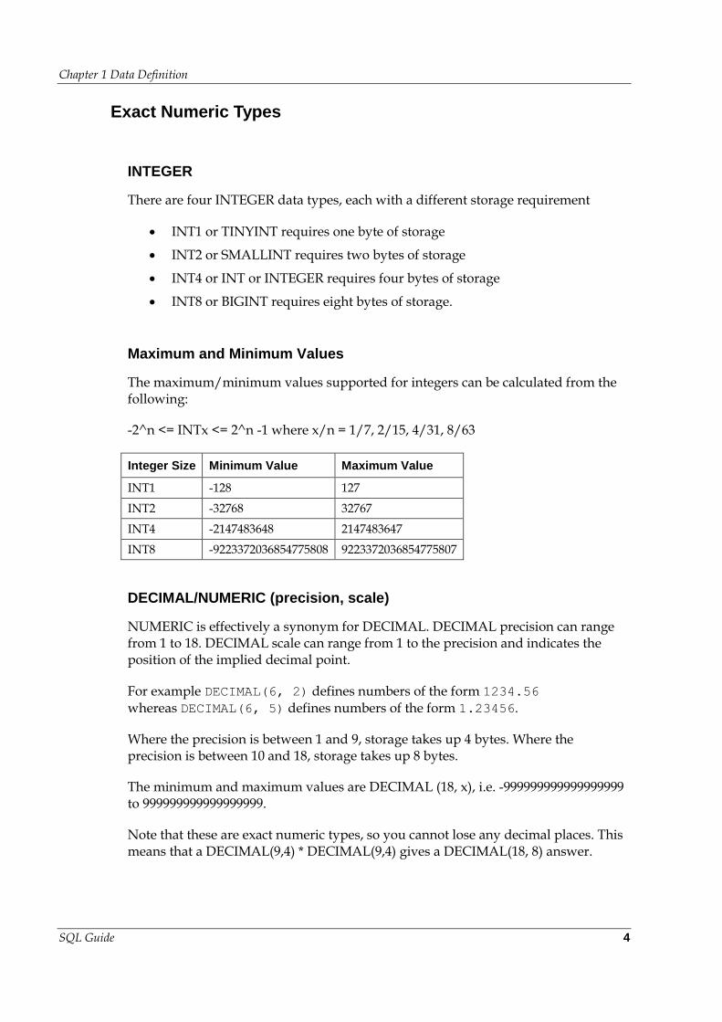
INTEGER
There are four INTEGER data types, each with a different storage requirement
INT1 or TINYINT requires one byte of storage
INT2 or SMALLINT requires two bytes of storage
INT4 or INT or INTEGER requires four bytes of storage
INT8 or BIGINT requires eight bytes of storage.
Maximum and Minimum Values
The maximum/minimum values supported for integers can be calculated from the following:
-2^n <= INTx <= 2^n -1 where x/n = 1/7, 2/15, 4/31, 8/63
Integer Size Minimum Value Maximum Value
INT1 -128 127
INT2 -32768 32767
INT4 -2147483648 2147483647
INT8 -9223372036854775808 9223372036854775807
DECIMAL/NUMERIC (precision, scale)
NUMERIC is effectively a synonym for DECIMAL. DECIMAL precision can range from 1 to 18. DECIMAL scale can range from 1 to the precision and indicates the position of the implied decimal point.
For example DECIMAL(6, 2) defines numbers of the form 1234.56 whereas DECIMAL(6, 5) defines numbers of the form 1.23456.
Where the precision is between 1 and 9, storage takes up 4 bytes. Where the precision is between 10 and 18, storage takes up 8 bytes.
The minimum and maximum values are DECIMAL (18, x), i.e. -999999999999999999 to 999999999999999999.
Note that these are exact numeric types, so you cannot lose any decimal places. This means that a DECIMAL(9,4) * DECIMAL(9,4) gives a DECIMAL(18, 8) answer.
Chapter 1 Data Definition
SQL Guide 5
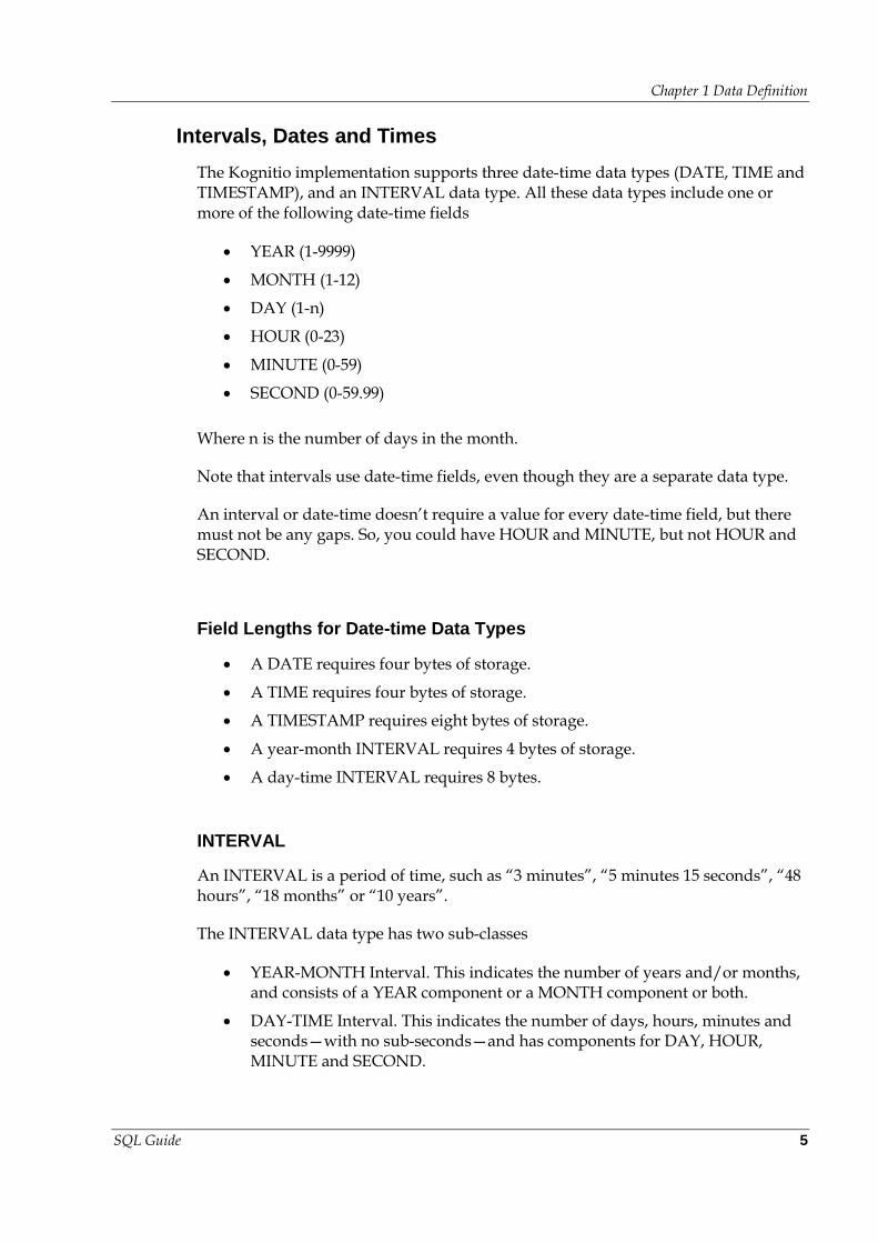
Intervals, Dates and Times
The Kognitio implementation supports three date-time data types (DATE, TIME and TIMESTAMP), and an INTERVAL data type. All these data types include one or more of the following date-time fields
YEAR (1-9999)
MONTH (1-12)
DAY (1-n)
HOUR (0-23)
MINUTE (0-59)
SECOND (0-59.99)
Where n is the number of days in the month.
Note that intervals use date-time fields, even though they are a separate data type.
An interval or date-time doesn’t require a value for every date-time field, but there must not be any gaps. So, you could have HOUR and MINUTE, but not HOUR and SECOND.
Field Lengths for Date-time Data Types
A DATE requires four bytes of storage.
A TIME requires four bytes of storage.
A TIMESTAMP requires eight bytes of storage.
A year-month INTERVAL requires 4 bytes of storage.
A day-time INTERVAL requires 8 bytes.
INTERVAL
An INTERVAL is a period of time, such as “3 minutes”, “5 minutes 15 seconds”, “48 hours”, “18 months” or “10 years”.
The INTERVAL data type has two sub-classes
YEAR-MONTH Interval. This indicates the number of years and/or months, and consists of a YEAR component or a MONTH component or both.
DAY-TIME Interval. This indicates the number of days, hours, minutes and seconds—with no sub-seconds—and has components for DAY, HOUR, MINUTE and SECOND.
Chapter 1 Data Definition
SQL Guide 6
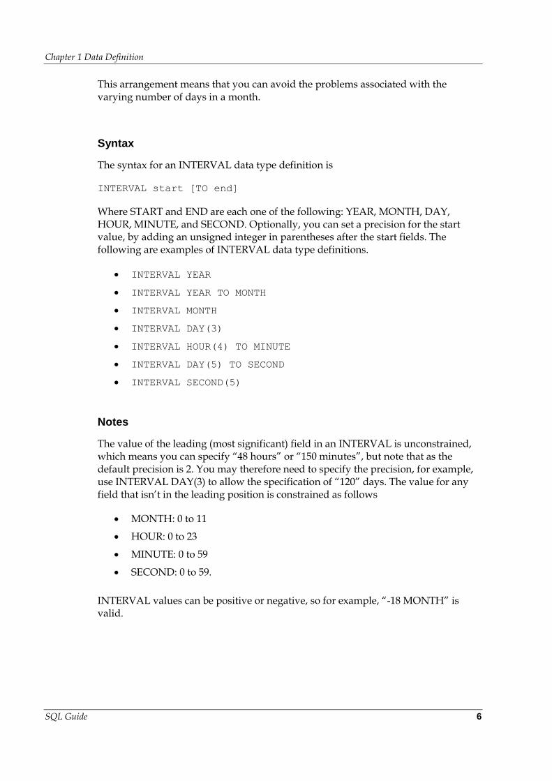
This arrangement means that you can avoid the problems associated with the varying number of days in a month.
Syntax
The syntax for an INTERVAL data type definition is
INTERVAL start [TO end]
Where START and END are each one of the following: YEAR, MONTH, DAY, HOUR, MINUTE, and SECOND. Optionally, you can set a precision for the start value, by adding an unsigned integer in parentheses after the start fields. The following are examples of INTERVAL data type definitions.
INTERVAL YEAR
INTERVAL YEAR TO MONTH
INTERVAL MONTH
INTERVAL DAY(3)
INTERVAL HOUR(4) TO MINUTE
INTERVAL DAY(5) TO SECOND
INTERVAL SECOND(5)
Notes
The value of the leading (most significant) field in an INTERVAL is unconstrained, which means you can specify “48 hours” or “150 minutes”, but note that as the default precision is 2. You may therefore need to specify the precision, for example, use INTERVAL DAY(3) to allow the specification of “120” days. The value for any field that isn’t in the leading position is constrained as follows
MONTH: 0 to 11
HOUR: 0 to 23
MINUTE: 0 to 59
SECOND: 0 to 59.
INTERVAL values can be positive or negative, so for example, “-18 MONTH” is valid.
Chapter 1 Data Definition
SQL Guide 7
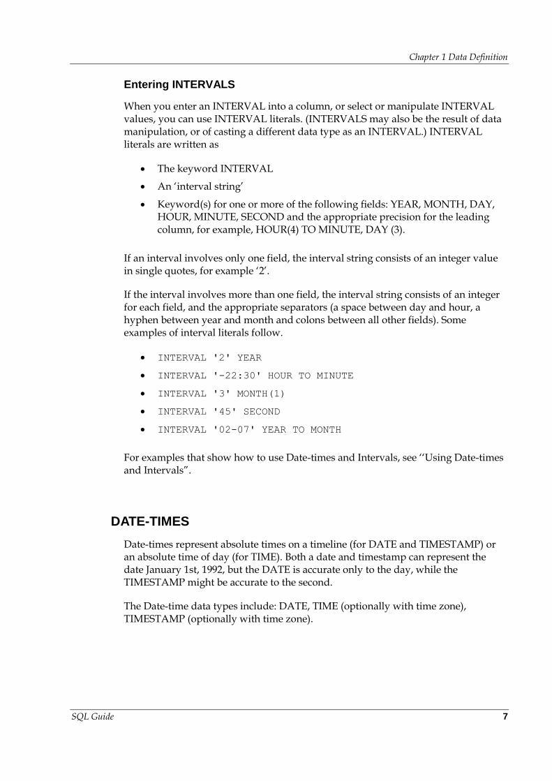
Entering INTERVALS
When you enter an INTERVAL into a column, or select or manipulate INTERVAL values, you can use INTERVAL literals. (INTERVALS may also be the result of data manipulation, or of casting a different data type as an INTERVAL.) INTERVAL literals are written as
The keyword INTERVAL
An ‘interval string’
Keyword(s) for one or more of the following fields: YEAR, MONTH, DAY, HOUR, MINUTE, SECOND and the appropriate precision for the leading column, for example, HOUR(4) TO MINUTE, DAY (3).
If an interval involves only one field, the interval string consists of an integer value in single quotes, for example ‘2’.
If the interval involves more than one field, the interval string consists of an integer for each field, and the appropriate separators (a space between day and hour, a hyphen between year and month and colons between all other fields). Some examples of interval literals follow.
INTERVAL '2' YEAR
INTERVAL '-22:30' HOUR TO MINUTE
INTERVAL '3' MONTH(1)
INTERVAL '45' SECOND
INTERVAL '02-07' YEAR TO MONTH
For examples that show how to use Date-times and Intervals, see ‘‘Using Date-times and Intervals”.
DATE-TIMES
Date-times represent absolute times on a timeline (for DATE and TIMESTAMP) or an absolute time of day (for TIME). Both a date and timestamp can represent the date January 1st, 1992, but the DATE is accurate only to the day, while the TIMESTAMP might be accurate to the second.
The Date-time data types include: DATE, TIME (optionally with time zone), TIMESTAMP (optionally with time zone).
Chapter 1 Data Definition
SQL Guide 8
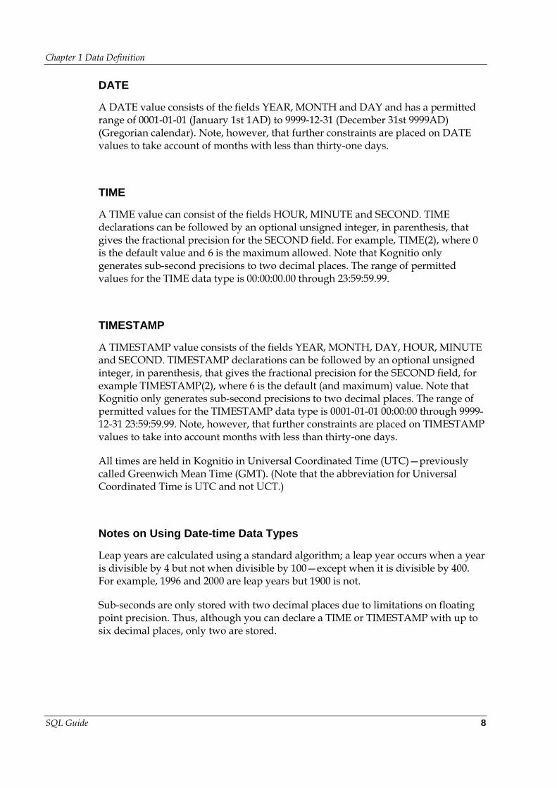
DATE
A DATE value consists of the fields YEAR, MONTH and DAY and has a permitted range of 0001-01-01 (January 1st 1AD) to 9999-12-31 (December 31st 9999AD) (Gregorian calendar). Note, however, that further constraints are placed on DATE values to take account of months with less than thirty-one days.
TIME
A TIME value can consist of the fields HOUR, MINUTE and SECOND. TIME declarations can be followed by an optional unsigned integer, in parenthesis, that gives the fractional precision for the SECOND field. For example, TIME(2), where 0 is the default value and 6 is the maximum allowed. Note that Kognitio only generates sub-second precisions to two decimal places. The range of permitted values for the TIME data type is 00:00:00.00 through 23:59:59.99.
TIMESTAMP
A TIMESTAMP value consists of the fields YEAR, MONTH, DAY, HOUR, MINUTE and SECOND. TIMESTAMP declarations can be followed by an optional unsigned integer, in parenthesis, that gives the fractional precision for the SECOND field, for example TIMESTAMP(2), where 6 is the default (and maximum) value. Note that Kognitio only generates sub-second precisions to two decimal places. The range of permitted values for the TIMESTAMP data type is 0001-01-01 00:00:00 through 9999-12-31 23:59:59.99. Note, however, that further constraints are placed on TIMESTAMP values to take into account months with less than thirty-one days.
All times are held in Kognitio in Universal Coordinated Time (UTC)—previously called Greenwich Mean Time (GMT). (Note that the abbreviation for Universal Coordinated Time is UTC and not UCT.)
Notes on Using Date-time Data Types
Leap years are calculated using a standard algorithm; a leap year occurs when a year is divisible by 4 but not when divisible by 100—except when it is divisible by 400. For example, 1996 and 2000 are leap years but 1900 is not.
Sub-seconds are only stored with two decimal places due to limitations on floating point precision. Thus, although you can declare a TIME or TIMESTAMP with up to six decimal places, only two are stored.
Chapter 1 Data Definition
SQL Guide 9
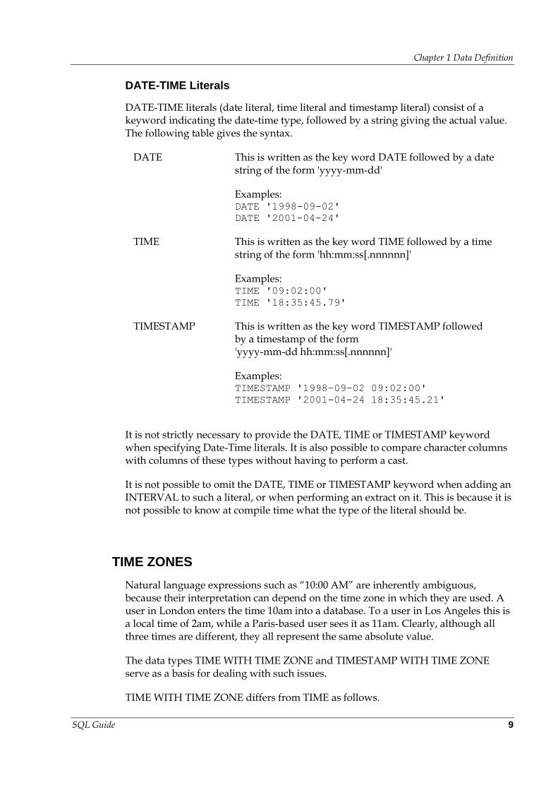
DATE-TIME Literals
DATE-TIME literals (date literal, time literal and timestamp literal) consist of a keyword indicating the date-time type, followed by a string giving the actual value. The following table gives the syntax.
DATE This is written as the key word DATE followed by a date string of the form 'yyyy-mm-dd'
Examples: DATE '1998-09-02'
DATE '2001-04-24'
TIME This is written as the key word TIME followed by a time string of the form 'hh:mm:ss[.nnnnnn]'
Examples: TIME '09:02:00'
TIME '18:35:45.79'
TIMESTAMP This is written as the key word TIMESTAMP followed by a timestamp of the form 'yyyy-mm-dd hh:mm:ss[.nnnnnn]'
Examples: TIMESTAMP '1998-09-02 09:02:00'
TIMESTAMP '2001-04-24 18:35:45.21'
It is not strictly necessary to provide the DATE, TIME or TIMESTAMP keyword when specifying Date-Time literals. It is also possible to compare character columns with columns of these types without having to perform a cast.
It is not possible to omit the DATE, TIME or TIMESTAMP keyword when adding an INTERVAL to such a literal, or when performing an extract on it. This is because it is not possible to know at compile time what the type of the literal should be.
TIME ZONES
Natural language expressions such as “10:00 AM” are inherently ambiguous, because their interpretation can depend on the time zone in which they are used. A user in London enters the time 10am into a database. To a user in Los Angeles this is a local time of 2am, while a Paris-based user sees it as 11am. Clearly, although all three times are different, they all represent the same absolute value.
The data types TIME WITH TIME ZONE and TIMESTAMP WITH TIME ZONE serve as a basis for dealing with such issues.
TIME WITH TIME ZONE differs from TIME as follows.
Chapter 1 Data Definition
SQL Guide 10
A TIME “without time zone” value is really a local time—it is the time given by a local clock. The value 10:00 AM in Los Angeles and London “compare equal” if they represent “without time zone values”, even though they denote different absolute times.
However, TIME WITH TIME ZONE values can be thought of as being corrected for time zone differences. So, values 10:00 in London and 02:00 in Los Angeles “compare equal” if they represent “with time zone” values, because they all denote the same absolute time.
TIME WITH TIME ZONE and TIMESTAMP WITH TIME ZONE are represented internally in terms of Universal Time Coordinated (UTC). To ensure that times are interpreted correctly for the local time, you can apply displacements to the internal time, and so produce the local time.
In all other respects, TIME WITH TIME ZONE and TIMESTAMP WITH TIME ZONE are similar to TIME and TIMESTAMP data types—they use Date Time fields, literals, and precision in the same way.
SET TIME ZONE
Use the SET TIME ZONE statement to specify which time zone the SQL session is running in.
Usage
SET TIME ZONE interval | LOCAL
Notes
If LOCAL is given then 0 is assumed, but any value given must be an INTERVAL HOUR TO MINUTE value (e.g. ‘hh:mm’).
Example – Setting the time zone to be PDT
To set the time zone to be 7 hours behind UTC (equivalent to PDT), use
SET TIME ZONE '-7:00'
1.2 NULLs
SQL represents the fact that some piece of information is missing by means of a special value called NULL. For example, you can say that the weight of some part, perhaps part P6, is NULL. What this means precisely is that

Chapter 1 Data Definition
SQL Guide 11
You know that part P6 exists
You know it has a weight, because all parts have a weight
You don’t know what the weight is.
In other words, you don’t know a genuine weight to enter in the Weight column for the row in the table for P6. Instead, you can mark the position as NULL, which is interpreted to mean, precisely, that the real value is unknown.
NULL is not the same as zero—the part in the example above has a weight, but you don’t know what it is.
NULLs take the data type of their column. You can CAST a NULL to any data type.
It is possible to omit explicitly casting a NULL when Kognitio can discern the type that the NULL should be cast to automatically. Setting the ci_strict parameter will prevent this implicit casting.
There are special SQL comparison operators IS NULL and IS NOT NULL for checking if a column or result of an expression is NULL.
The special OUTER JOIN construct exists to allow rows containing NULLs to participate in the results of a join. Normally an INNER JOIN will discard such rows.
A detailed discussion of the effects of NULLs throughout the SQL language is beyond the scope of this reference guide. Where appropriate individual functions and operators will highlight the impact of NULLs on them.
Refer to the SQL Standard for additional information on NULLs.
1.3 Schemas, Tables, Views and Images
Overview
Conceptually a relational database is simply a collection of base tables containing an unordered collection of rows of data. Each row consists of one or more columns. It is also possible to define views of the base table(s), which are simply definitions of objects based on the underlying base table(s).
SQL objects such as tables and views are always created within the context of a schema and are considered to "belong to" the schema in question. SQL operations can span schemas.
Chapter 1 Data Definition
SQL Guide 12
The Kognitio architecture is designed so that images of tables and views are loaded into RAM for rapid access. A series of Kognitio specific SQL extensions exist to create and manipulate these images.
ALTER SYSTEM
Use the ALTER SYSTEM statement to alter certain characteristics of all the schemas of the system.
Usage
ALTER SYSTEM SET
DEFAULT CHARACTER SET TO character-set
ALTER SYSTEM SET
SLABS TO {ALL | slab-list} [MIGRATE [DEFRAG]]
Notes
See chapter 8 for details of supported character sets.
See the Kognitio Guide for details of disk store slabs.
CREATE SCHEMA
The CREATE SCHEMA statement allows a user to create a schema.
Usage
CREATE SCHEMA
schema-name [DEFAULT CHARACTER SET character-set] |
AUTHORIZATION user-name |
schema-name AUTHORIZATION user-name
[SET SLABS TO {ALL | slab-list}]
Notes
This lets a user create a schema for someone else, providing they have the INSERT privilege on IPE_SCHEMA. The user creating a schema must have the CREATE SCHEMA privilege. (Typically, creating a schema is done by SYS when new users are created.)
Chapter 1 Data Definition
SQL Guide 13
See “Example – Creating and Dropping Schemas” on page 14 for an example of CREATE SCHEMA use.
See chapter 8 for details of supported character sets.
See the Kognitio Guide for details of disk store slabs.
ALTER SCHEMA
Use the ALTER SCHEMA statement to alter certain characteristics of a schema.
Usage
ALTER SCHEMA schema-name SET
DEFAULT CHARACTER SET TO character-set
ALTER SCHEMA schema-name SET
SLABS TO {ALL | SYSTEM DEFAULT | slab-list} [MIGRATE [DEFRAG]]
Notes
See chapter 8 for details of supported character sets.
See the Kognitio Guide for details of disk store slabs.
DROP SCHEMA
Use the DROP SCHEMA statement to drop existing schemas.
Usage
DROP SCHEMA schema-name {CASCADE | RESTRICT}
Notes
SYS is the only person who can drop any schema on Kognitio. Other users can only issue the DROP SCHEMA command for a schema that they own.
The RESTRICT keyword limits the command, so that it only drops schemas that are empty.
Chapter 1 Data Definition
SQL Guide 14
The CASCADE keyword drops all database objects in the specified schema, and any
referenced in other schemas before dropping the schema itself.
Example – Creating and Dropping Schemas
The following example illustrates how a table in one schema with a foreign key reference to a table in another schema is affected when the referenced table is modified and then the schema is dropped. See “CREATE TABLE” on page 16 for details of CREATE TABLE and referential integrity.
-- Create a schema and a table. Insert a couple of rows.
CREATE SCHEMA s1;
SET SCHEMA s1;
CREATE TABLE t1(i INT NOT NULL PRIMARY KEY,
s Varchar(255));
INSERT INTO t1 VALUES (1, 'one');
INSERT INTO t1 VALUES (2, 'two');
-- Create a second schema and table that references the first.
-- Again add a couple of rows and show what happens when the
-- reference doesn’t exist.
SET SCHEMA DEFAULT;
CREATE SCHEMA s2;
SET SCHEMA s2;
CREATE TABLE t2(x INT PRIMARY KEY NOT NULL,
i INT,
FOREIGN KEY (i) REFERENCES s1.t1
ON DELETE SET NULL);
INSERT INTO t2 VALUES (1, 1);
INSERT INTO t2 VALUES (2, 2);
INSERT INTO t2 VALUES (2, 22);
CI8028: Referential integrity row does not exist
-- Confirm table contents and show what happens when a row
-- is deleted from t1 with our specified on delete clause.
-- Note that when the row is deleted, we are correctly
-- informed that 2 rows have been affected.
SELECT * FROM t2;
X : I
1, 1
2, 2
SET SCHEMA s1;
SELECT * FROM t1;
I : S
1, one
2, two
DELETE FROM t1 WHERE i = 2;
2 rows affected.
SELECT * FROM t1;
I : S
1, one
Chapter 1 Data Definition
SQL Guide 15
SET SCHEMA s2
SELECT * FROM t2;
X : I
1, 1
2, <<<NULL>>>
-- Now drop the first schema and see what happens to our table
-- that referenced a table within it
SET SCHEMA DEFAULT;
DROP SCHEMA s1 CASCADE;
SET SCHEMA s2
SELECT * FROM t2;
CI3013: Table S2.T2 does not exist
SET SCHEMA
Use the SET SCHEMA statement to set your default schema.
Usage
SET SCHEMA {DEFAULT | schema-name}
Notes
When the System Administrator creates a user identity for you, they either give you your own schema or allocate you to an existing schema. Subsequently, this schema is taken as your "default" schema, and any submission against a specified table searches the default schema. You can change the default schema for the current session with the SET SCHEMA command.
Before using the SET SCHEMA command, you can refer to tables in your own schema without using a schema prefix, giving
mytable
But when you refer to tables in the schema you intend to set as default, you need to include the schema name, e.g.
yourschema.yourtable
After using the SET SCHEMA command, e.g.
SET SCHEMA yourschema
You can refer to the tables in the new default schema without a schema prefix, e.g.
yourtable
Chapter 1 Data Definition
SQL Guide 16
But you must add the schema prefix when referring to tables in your own schema, e.g.
myschema.mytable
The new schema remains as the default until
The session is disconnected, or
You issue another SET SCHEMA statement.
Re-allocating the default schema doesn’t automatically give access to tables in that schema—the privilege constraints still apply.
It isn’t necessary to specify the default schema name, as this is allocated at the time of user installation, and is automatically restored.
See “Example – Creating and Dropping Schemas” on page 14 for additional examples of SET SCHEMA use.
CREATE TABLE
In its basic form the CREATE TABLE statement creates a new table and defines the columns in it. By default, on a Kognitio a random image of the table is also placed in RAM (this default behaviour can be modified by using the Kognitio system parameter "def_table_loc").
The user can also specify if and how a table should be distributed in RAM, and also generate the table definition from a SELECT statement. This SELECT statement can also optionally be used to populate the table. It is also possible to create RAM Only Temporary Tables (ROTTs).
Usage
CREATE [RAM ONLY] TABLE table
[({column-name [data-type]
[{NOT NULL | NULL}]
[{UNIQUE | PRIMARY KEY}]
[references-spec]
[DEFAULT default-spec]
[CHECK (constraint-expression)]
| UNIQUE ({column-name},...)
| PRIMARY KEY ({column-name},...)
| FOREIGN KEY ({column-name},...)
| CHECK ((constraint-expression),...)]
[IMAGE ({column-name},...)]
[DISK | RANDOM | REPLICATED | HASHED [ON] ({column-name},...)
[RANDOM | REPLICATED [rvc-list | VALUES (hash-value-list)]]
Chapter 1 Data Definition
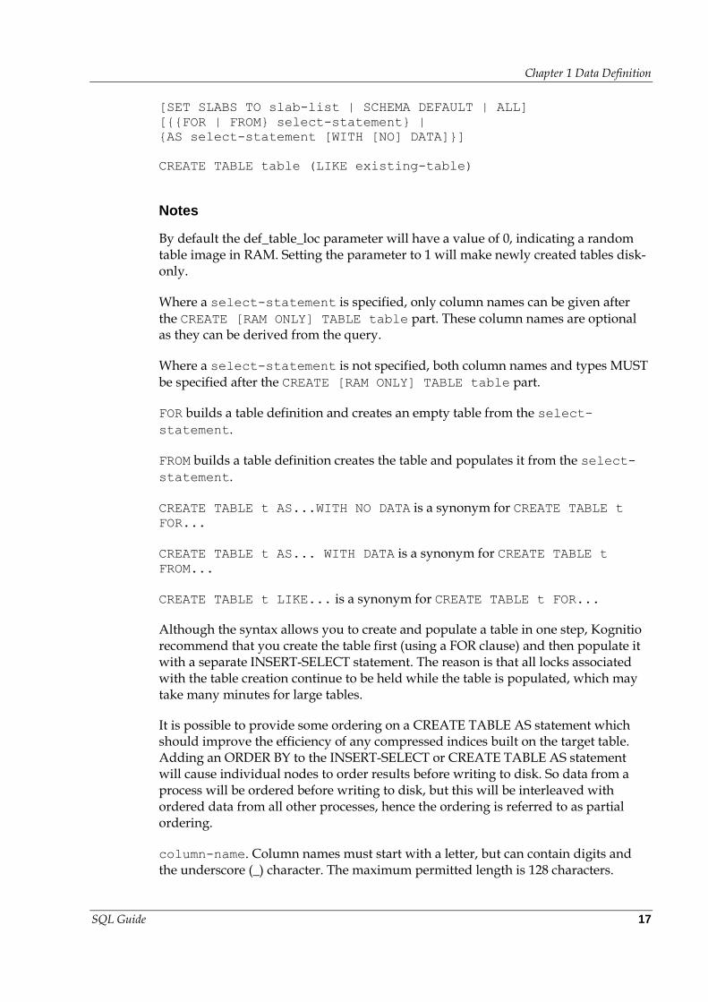
SQL Guide 17
[SET SLABS TO slab-list | SCHEMA DEFAULT | ALL]
[{{FOR | FROM} select-statement} |
{AS select-statement [WITH [NO] DATA]}]
CREATE TABLE table (LIKE existing-table)
Notes
By default the def_table_loc parameter will have a value of 0, indicating a random table image in RAM. Setting the parameter to 1 will make newly created tables disk-only.
Where a select-statement is specified, only column names can be given after the CREATE [RAM ONLY] TABLE table part. These column names are optional as they can be derived from the query.
Where a select-statement is not specified, both column names and types MUST be specified after the CREATE [RAM ONLY] TABLE table part.
FOR builds a table definition and creates an empty table from the select-statement.
FROM builds a table definition creates the table and populates it from the select-statement.
CREATE TABLE t AS...WITH NO DATA is a synonym for CREATE TABLE t FOR...
CREATE TABLE t AS... WITH DATA is a synonym for CREATE TABLE t FROM...
CREATE TABLE t LIKE... is a synonym for CREATE TABLE t FOR...
Although the syntax allows you to create and populate a table in one step, Kognitio recommend that you create the table first (using a FOR clause) and then populate it with a separate INSERT-SELECT statement. The reason is that all locks associated with the table creation continue to be held while the table is populated, which may take many minutes for large tables.
It is possible to provide some ordering on a CREATE TABLE AS statement which should improve the efficiency of any compressed indices built on the target table. Adding an ORDER BY to the INSERT-SELECT or CREATE TABLE AS statement will cause individual nodes to order results before writing to disk. So data from a process will be ordered before writing to disk, but this will be interleaved with ordered data from all other processes, hence the ordering is referred to as partial ordering.
column-name. Column names must start with a letter, but can contain digits and the underscore (_) character. The maximum permitted length is 128 characters.
Chapter 1 Data Definition
SQL Guide 18
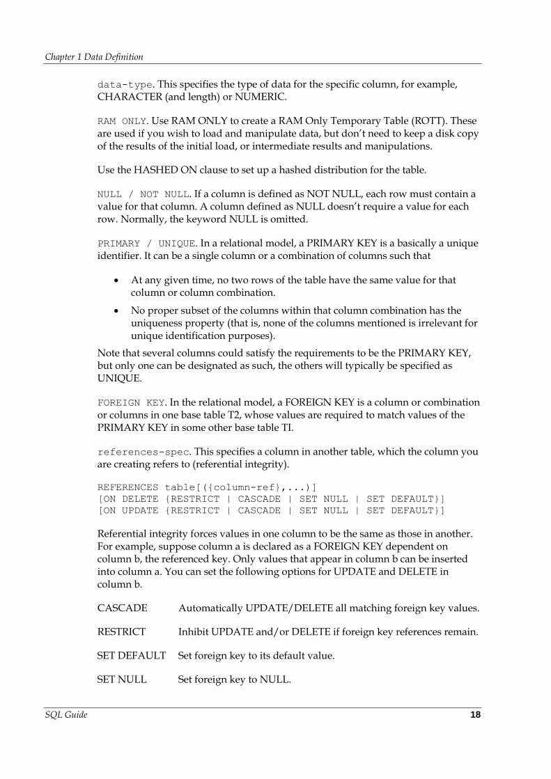
data-type. This specifies the type of data for the specific column, for example, CHARACTER (and length) or NUMERIC.
RAM ONLY. Use RAM ONLY to create a RAM Only Temporary Table (ROTT). These are used if you wish to load and manipulate data, but don’t need to keep a disk copy of the results of the initial load, or intermediate results and manipulations.
Use the HASHED ON clause to set up a hashed distribution for the table.
NULL / NOT NULL. If a column is defined as NOT NULL, each row must contain a value for that column. A column defined as NULL doesn’t require a value for each row. Normally, the keyword NULL is omitted.
PRIMARY / UNIQUE. In a relational model, a PRIMARY KEY is a basically a unique identifier. It can be a single column or a combination of columns such that
At any given time, no two rows of the table have the same value for that column or column combination.
No proper subset of the columns within that column combination has the uniqueness property (that is, none of the columns mentioned is irrelevant for unique identification purposes).
Note that several columns could satisfy the requirements to be the PRIMARY KEY, but only one can be designated as such, the others will typically be specified as UNIQUE.
FOREIGN KEY. In the relational model, a FOREIGN KEY is a column or combination or columns in one base table T2, whose values are required to match values of the PRIMARY KEY in some other base table TI.
references-spec. This specifies a column in another table, which the column you are creating refers to (referential integrity).
REFERENCES table[({column-ref},...)]
[ON DELETE {RESTRICT | CASCADE | SET NULL | SET DEFAULT}]
[ON UPDATE {RESTRICT | CASCADE | SET NULL | SET DEFAULT}]
Referential integrity forces values in one column to be the same as those in another. For example, suppose column a is declared as a FOREIGN KEY dependent on column b, the referenced key. Only values that appear in column b can be inserted into column a. You can set the following options for UPDATE and DELETE in column b.
CASCADE Automatically UPDATE/DELETE all matching foreign key values.
RESTRICT Inhibit UPDATE and/or DELETE if foreign key references remain.
SET DEFAULT Set foreign key to its default value.
SET NULL Set foreign key to NULL.
Chapter 1 Data Definition
SQL Guide 19
Note that if you want to use referential integrity to maintain integrity during INSERT, UPDATE and DELETE operations, all columns of all tables involved must be in RAM.
default-spec. This specifies a default value to be placed in a column, where the user doesn’t provide a value on INSERT. This value can be a literal, a literal expression, or the keyword NULL. Note that IMPORT doesn’t use default-specs.
CHECK constraint-expression. The CREATE TABLE statement can incorporate a CHECK constraint, which can apply to multiple columns (table level) or to a single column (column level). Note that a CHECK constraint cannot reference another table.
Note that IMPORT doesn’t enforce CHECK constraints.
See the Kognitio Guide for details of disk store slabs.
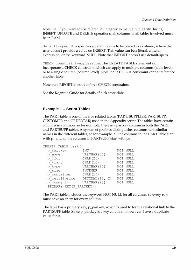
Example 1 – Script Tables
The PART table is one of the five related tables (PART, SUPPLIER, PARTSUPP, CUSTOMER and ORDERTAB) used in the Appendix script. The tables have certain columns in common, so for example, there is a partkey column in both the PART and PARTSUPP tables. A system of prefixes distinguishes columns with similar names in the different tables, so for example, all the columns in the PART table start with p_ and all the columns in PARTSUPP start with ps_.
CREATE TABLE part(
p_partkey INT NOT NULL,
p_name VARCHAR(55) NOT NULL,
p_mfgr CHAR(25) NOT NULL,
p_brand CHAR(10) NOT NULL,
p_type VARCHAR(25) NOT NULL,
p_size INTEGER NOT NULL,
p_container CHAR(10) NOT NULL,
p_retailprice DECIMAL(12, 2) NOT NULL,
p_comment VARCHAR(23) NOT NULL,
PRIMARY KEY(P_PARTKEY))
The PART table includes the keyword NOT NULL for all columns, so every row must have an entry for every column.
The table has a primary key, p_partkey, which is used to form a relational link to the PARTSUPP table. Since p_partkey is a key column, no rows can have a duplicate value for it.
Chapter 1 Data Definition
SQL Guide 20
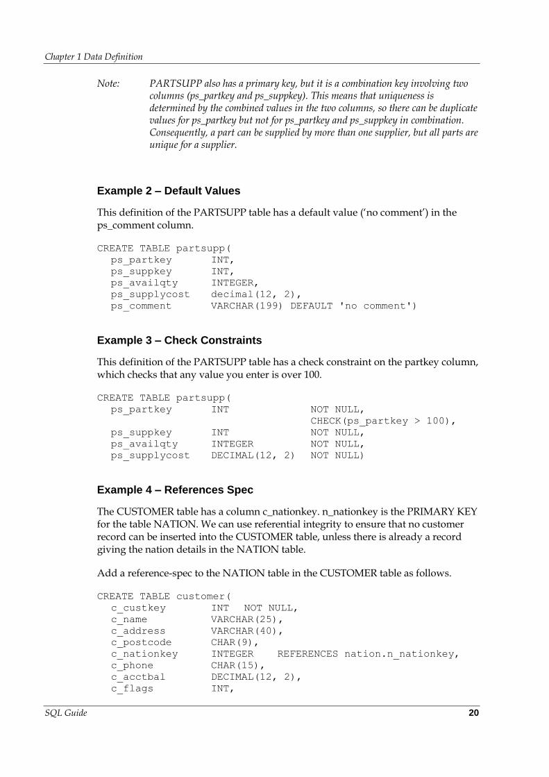
Note: PARTSUPP also has a primary key, but it is a combination key involving two columns (ps_partkey and ps_suppkey). This means that uniqueness is determined by the combined values in the two columns, so there can be duplicate values for ps_partkey but not for ps_partkey and ps_suppkey in combination. Consequently, a part can be supplied by more than one supplier, but all parts are unique for a supplier.
Example 2 – Default Values
This definition of the PARTSUPP table has a default value (‘no comment’) in the ps_comment column.
CREATE TABLE partsupp(
ps_partkey INT,
ps_suppkey INT,
ps_availqty INTEGER,
ps_supplycost decimal(12, 2),
ps_comment VARCHAR(199) DEFAULT 'no comment')
Example 3 – Check Constraints
This definition of the PARTSUPP table has a check constraint on the partkey column, which checks that any value you enter is over 100.
CREATE TABLE partsupp(
ps_partkey INT NOT NULL,
CHECK(ps_partkey > 100),
ps_suppkey INT NOT NULL,
ps_availqty INTEGER NOT NULL,
ps_supplycost DECIMAL(12, 2) NOT NULL)
Example 4 – References Spec
The CUSTOMER table has a column c_nationkey. n_nationkey is the PRIMARY KEY for the table NATION. We can use referential integrity to ensure that no customer record can be inserted into the CUSTOMER table, unless there is already a record giving the nation details in the NATION table.
Add a reference-spec to the NATION table in the CUSTOMER table as follows.
CREATE TABLE customer(
c_custkey INT NOT NULL,
c_name VARCHAR(25),
c_address VARCHAR(40),
c_postcode CHAR(9),
c_nationkey INTEGER REFERENCES nation.n_nationkey,
c_phone CHAR(15),
c_acctbal DECIMAL(12, 2),
c_flags INT,
Chapter 1 Data Definition
SQL Guide 21
PRIMARY KEY(c_custkey))
Notes: This can also be done with a FOREIGN KEY definition at the end of the table definition.
There is a performance penalty if referential integrity is used.
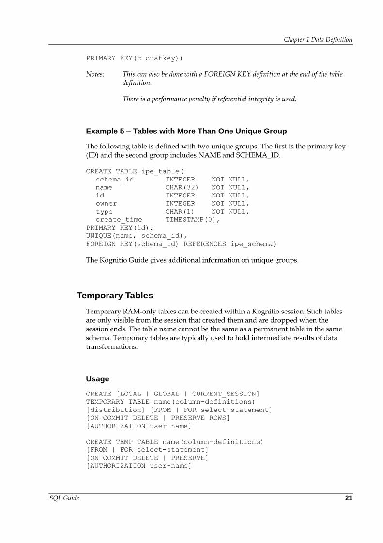
Example 5 – Tables with More Than One Unique Group
The following table is defined with two unique groups. The first is the primary key (ID) and the second group includes NAME and SCHEMA_ID.
CREATE TABLE ipe_table(
schema_id INTEGER NOT NULL,
name CHAR(32) NOT NULL,
id INTEGER NOT NULL,
owner INTEGER NOT NULL,
type CHAR(1) NOT NULL,
create_time TIMESTAMP(0),
PRIMARY KEY(id),
UNIQUE(name, schema_id),
FOREIGN KEY(schema_id) REFERENCES ipe_schema)
The Kognitio Guide gives additional information on unique groups.
Temporary Tables
Temporary RAM-only tables can be created within a Kognitio session. Such tables are only visible from the session that created them and are dropped when the session ends. The table name cannot be the same as a permanent table in the same schema. Temporary tables are typically used to hold intermediate results of data transformations.
Usage
CREATE [LOCAL | GLOBAL | CURRENT_SESSION]
TEMPORARY TABLE name(column-definitions)
[distribution] [FROM | FOR select-statement]
[ON COMMIT DELETE | PRESERVE ROWS]
[AUTHORIZATION user-name]
CREATE TEMP TABLE name(column-definitions)
[FROM | FOR select-statement]
[ON COMMIT DELETE | PRESERVE]
[AUTHORIZATION user-name]
Chapter 1 Data Definition
SQL Guide 22
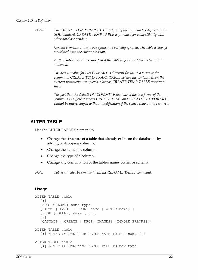
Notes: The CREATE TEMPORARY TABLE form of the command is defined in the SQL standard. CREATE TEMP TABLE is provided for compatibility with other database vendors.
Certain elements of the above syntax are actually ignored. The table is always associated with the current session.
Authorisation cannot be specified if the table is generated from a SELECT statement.
The default value for ON COMMIT is different for the two forms of the command: CREATE TEMPORARY TABLE deletes the contents when the current transaction completes, whereas CREATE TEMP TABLE preserves them.
The fact that the default ON COMMIT behaviour of the two forms of the command is different means CREATE TEMP and CREATE TEMPORARY cannot be interchanged without modification if the same behaviour is required.
ALTER TABLE
Use the ALTER TABLE statement to
Change the structure of a table that already exists on the database—by adding or dropping columns,
Change the name of a column,
Change the type of a column,
Change any combination of the table's name, owner or schema.
Note: Tables can also be renamed with the RENAME TABLE command.
Usage
ALTER TABLE table
[(]
{ADD [COLUMN] name type
[FIRST | LAST | BEFORE name | AFTER name} |
{DROP [COLUMN] name [,...]
[)]
[CASCADE [{CREATE | DROP} IMAGES] [IGNORE ERRORS]]]
ALTER TABLE table
[(] ALTER COLUMN name ALTER NAME TO new-name [)]
ALTER TABLE table
[(] ALTER COLUMN name ALTER TYPE TO new-type
Chapter 1 Data Definition
SQL Guide 23
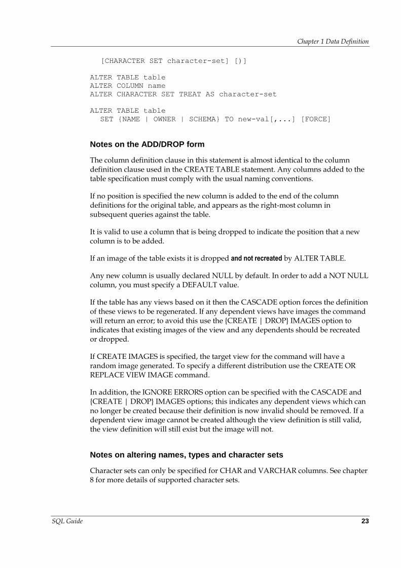
[CHARACTER SET character-set] [)]
ALTER TABLE table
ALTER COLUMN name
ALTER CHARACTER SET TREAT AS character-set
ALTER TABLE table
SET {NAME | OWNER | SCHEMA} TO new-val[,...] [FORCE]
Notes on the ADD/DROP form
The column definition clause in this statement is almost identical to the column definition clause used in the CREATE TABLE statement. Any columns added to the table specification must comply with the usual naming conventions.
If no position is specified the new column is added to the end of the column definitions for the original table, and appears as the right-most column in subsequent queries against the table.
It is valid to use a column that is being dropped to indicate the position that a new column is to be added.
If an image of the table exists it is dropped and not recreated by ALTER TABLE.
Any new column is usually declared NULL by default. In order to add a NOT NULL column, you must specify a DEFAULT value.
If the table has any views based on it then the CASCADE option forces the definition of these views to be regenerated. If any dependent views have images the command will return an error; to avoid this use the {CREATE | DROP} IMAGES option to indicates that existing images of the view and any dependents should be recreated or dropped.
If CREATE IMAGES is specified, the target view for the command will have a random image generated. To specify a different distribution use the CREATE OR REPLACE VIEW IMAGE command.
In addition, the IGNORE ERRORS option can be specified with the CASCADE and {CREATE | DROP} IMAGES options; this indicates any dependent views which can no longer be created because their definition is now invalid should be removed. If a dependent view image cannot be created although the view definition is still valid, the view definition will still exist but the image will not.
Notes on altering names, types and character sets
Character sets can only be specified for CHAR and VARCHAR columns. See chapter 8 for more details of supported character sets.
Chapter 1 Data Definition
SQL Guide 24
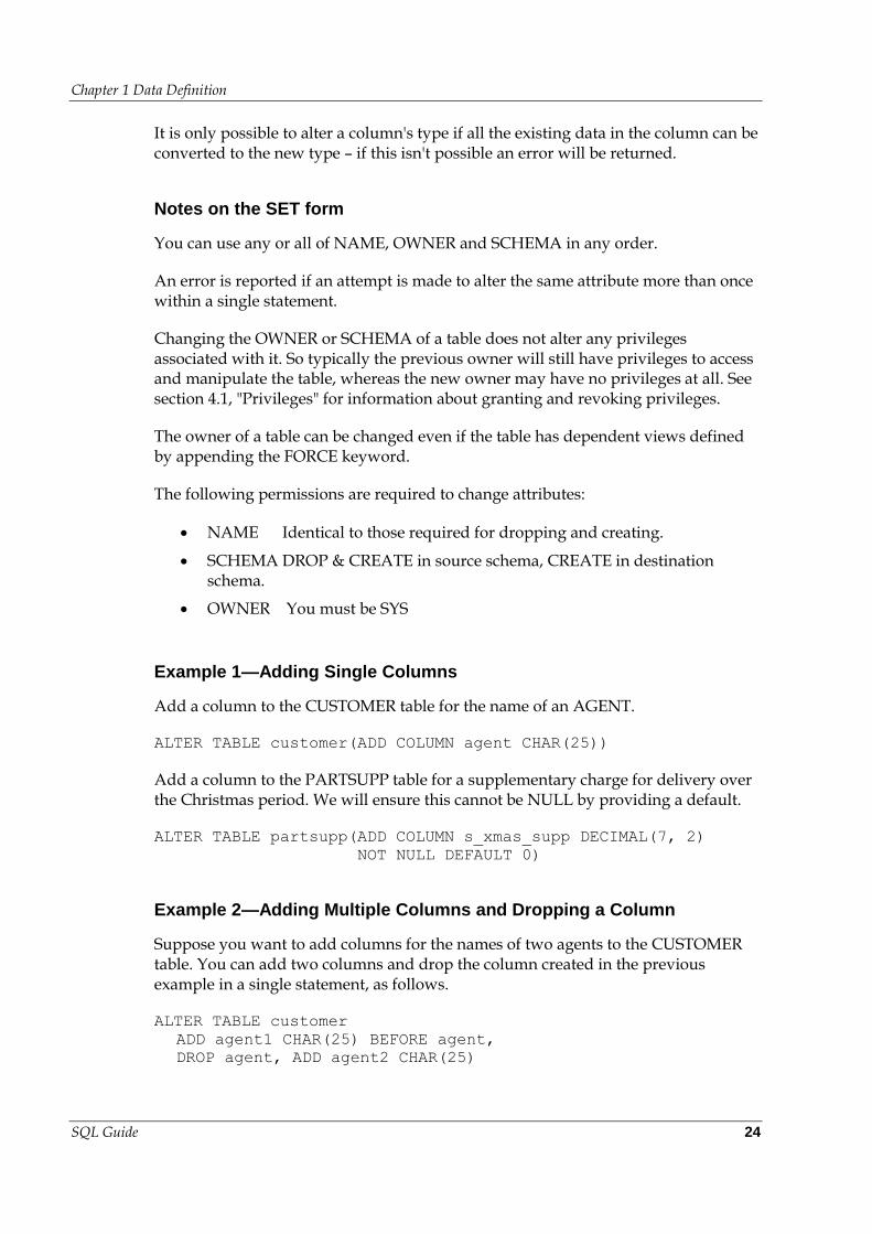
It is only possible to alter a column's type if all the existing data in the column can be converted to the new type – if this isn't possible an error will be returned.
Notes on the SET form
You can use any or all of NAME, OWNER and SCHEMA in any order.
An error is reported if an attempt is made to alter the same attribute more than once within a single statement.
Changing the OWNER or SCHEMA of a table does not alter any privileges associated with it. So typically the previous owner will still have privileges to access and manipulate the table, whereas the new owner may have no privileges at all. See section 4.1, "Privileges" for information about granting and revoking privileges.
The owner of a table can be changed even if the table has dependent views defined by appending the FORCE keyword.
The following permissions are required to change attributes:
NAME Identical to those required for dropping and creating.
SCHEMA DROP & CREATE in source schema, CREATE in destination schema.
OWNER You must be SYS
Example 1—Adding Single Columns
Add a column to the CUSTOMER table for the name of an AGENT.
ALTER TABLE customer(ADD COLUMN agent CHAR(25))
Add a column to the PARTSUPP table for a supplementary charge for delivery over the Christmas period. We will ensure this cannot be NULL by providing a default.
ALTER TABLE partsupp(ADD COLUMN s_xmas_supp DECIMAL(7, 2)
NOT NULL DEFAULT 0)
Example 2—Adding Multiple Columns and Dropping a Column
Suppose you want to add columns for the names of two agents to the CUSTOMER table. You can add two columns and drop the column created in the previous example in a single statement, as follows.
ALTER TABLE customer
ADD agent1 CHAR(25) BEFORE agent,
DROP agent, ADD agent2 CHAR(25)
Chapter 1 Data Definition
SQL Guide 25
Example 3—Renaming and Changing Owner and Containing Schema
The following renames the CUSTOMER table and changes the owner and schema attributes.
ALTER TABLE customer SET
NAME TO newcustomers,
OWNER TO presales,
SCHEMA TO sales
Example 4—Altering the Type and Character Set of a Column
The following alters the type and character set of the agent1 column that was added to the CUSTOMER table above.
ALTER TABLE customer
ALTER COLUMN agent1 ALTER TYPE TO VARCHAR(40)
CHARACTER SET UTF8
RENAME TABLE
Use the RENAME TABLE statement to rename a table:
Usage
RENAME TABLE oldname TO newname
CREATE TABLE IMAGE
Use the CREATE TABLE IMAGE statement to set up a RAM image of a table or selected columns and/or rows from a table. Any changes to the table are reflected in RAM as well as on disk. Because the image is in RAM, queries run significantly faster on a table image. For more information on table images, see the Kognitio Guide.
Note: When you create a table, by default, a RAM image is also created. It is only possible to create one table image of any particular table at any one time.
Usage
CREATE TABLE IMAGE table[(column-list)]
[WHERE search-condition]
CREATE TABLE IMAGE table REPLICATED [WHERE search-condition]
Chapter 1 Data Definition
SQL Guide 26
CREATE TABLE IMAGE table[(column-list)]
HASHED [ON] (column-list)
[WHERE search-condition]
CREATE TABLE IMAGE table[(column-list)]
HASHED [ON](column-list) RANDOM | REPLICATED
[IN (select-list) | VALUES(RVC-list) | (hash-value-list)]
[WHERE search-condition]
Notes
On Kognitio, data is normally distributed randomly across all RAMStores. The Kognitio extensions to SQL provide alternate distributions that allow certain joins to operate more efficiently. These distributions are hashed and replicated.
Use the HASHED clause to select a column (or columns) to use as a key to hash distribute an image across the available RAM. If two table/view images have columns with identical values and each is selected as a hash key so that both images are hash distributed, then pairs of rows with the same key from the two images are placed on the same RAMStore. Any query involving a join between the two hashed images based on hashed column(s) runs efficiently, because the rows being joined are located together on the same RAMStore.
If both the table images are dropped, the compiler may create temporary copies of the hashed table images for you, depending on the query and the data demographics.
If 1 or more values occur far more frequently than others, for example NULL or a default, then the hashed image may be skewed in memory, and occupy far more space on one RAMStore than on the others (assuming that it fits at all).
The REPLICATED clause specifies that a complete copy of a selected table is loaded onto every RAMStore. It is most commonly used to perform a join between two tables, where one table is very large and the second (replicated) table is much smaller. A table image can be both fragmented (see below) and replicated.
Partial distributions handle joins when a large table is severely skewed. Partial hashing provides an alternative to straightforward hashing. There are two forms
Partial hashed/random
Partial hashed/replicated.
Partial hashing makes use of a list of exception values, which identify the values that are causing the skewing. Most rows hash in the same way as a normal hashed distribution, but if a value is an exception, then depending on the type of partial distribution, it is either
Given to a random RAMStore (partial hashed/random), or
Replicated (Partial hashed/replicated).
Chapter 1 Data Definition
SQL Guide 27
The final form of the statement in the above usage section is used to create partially hashed distributions. One way to specify the exception values is as an RVC-list, meaning that individual values are enclosed in parentheses. This allows distributions that are hashed on more than one column to be defined. This is illustrated by the following extract from a worked example in the Kognitio Guide that discusses partial distributions in detail.
CREATE VIEW IMAGE telco_sumview
HASHED ON(Orig_State)
REPLICATED VALUES(('NY'), ('CA'), ('PA'), ('NJ'),
('IL'), ('MD'), ('MA'), ('TX'))
It is also possible to specify the exception values via a SELECT statement. This is frequently the best way to identify the values in a production environment where the distribution of the underlying data may be constantly changing. For example:
CREATE VIEW IMAGE telco_sumview
HASHED ON(Orig_State)
REPLICATED IN (
SELECT Orig_State FROM (
SELECT Orig_State, COUNT(Orig_State) cs, MAX(x) mx
FROM telco_demo,
(SELECT COUNT(*) FROM telco_demo) AS dt(x)
GROUP BY Orig_State) AS dt2
WHERE 100.0 * cs / mx > 5.0);
SQL does not permit the use of aliases in the WHERE or HAVING clauses of a SELECT, this could result in some expressions being repeated; making the SQL more verbose and prone to error if the expressions are complex and/or regularly changed. To avoid this problem the above example uses derived tables so that the expressions are specified only once.
HAVING clauses and derived tables are both described later in this document and in the Kognitio Guide.
Fragmented Table Images
There may be insufficient space to fit the complete image of a large table into RAM. If this happens, you can make a fragmented image of the table, which loads only the most frequently accessed columns into RAM and leaves the rest on disk. The data on disk is still accessible.
Note that it is good practice to use fragmentation; since the less data there is in RAM the faster it can be scanned. So, for example, avoid loading large comment fields into RAM unnecessarily. Remember that other users may be affected if you use too much RAM.
Hashed and replicated images, partial hashing, and fragmented images are discussed in detail in the Kognitio Guide.
Chapter 1 Data Definition
SQL Guide 28
Horizontally Fragmented Table Images
It is possible to supply a WHERE clause when creating a table image. This allows for a subset of the rows in the table to be imaged in RAM (e.g. the most recent three months of data).
All operations can be run against the table as usual, but if the operation only needs to use the data in RAM it will be much quicker than if no image was involved, and the RAM footprint for the system will be much lower than if a full image was used.
Example 1 – Dropping and Creating a Table Image
Create a table image of the CUSTOMER table. When you create the table, by default a RAM image is created at the same time, so this image must be dropped before you create another one. (There are various reasons for dropping an image, including making space available for an image of another large table or view, or wishing to instantiate a replicated or hashed image as in Examples 2 and 3.)
DROP TABLE IMAGE customer
Once the image has been dropped, you can give the CREATE TABLE IMAGE command to create the image with a different distribution.
CREATE TABLE IMAGE customer REPLICATED
Note: It is possible to specify the required table image distribution when the table is created, however the default behaviour will still be as specified above.
Example 2 – Replicated Table Images
The CUSTOMER and SUPPLIER tables each have a column for nation (s_nationkey and c_nationkey), with an INT data type. The NATION table can be used to map country names to these identifiers. Since the NATION table will be small a replicated image is appropriate.
CREATE TABLE IMAGE nation REPLICATED
Example 3 – Hashed Distribute Two Fragmented Table Images
This example creates fragmented, hashed tables images for the PART and PARTSUPP tables. The columns part.p_partkey and partsupp.ps_partkey are the key columns used to hash distribute the tables. Pairs of rows with the same hash key from the two tables are placed on the same RAMStores and so these tables will be distributed in a way suitable for joining on their partkey columns.
You must drop existing table images for PART and PARTSUPP before you can create the hashed table images, so the following may be necessary.
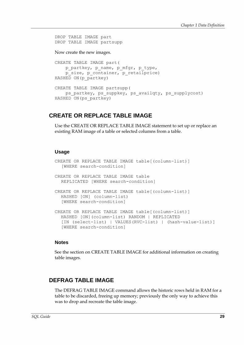
Chapter 1 Data Definition
SQL Guide 29
DROP TABLE IMAGE part
DROP TABLE IMAGE partsupp
Now create the new images.
CREATE TABLE IMAGE part(
p_partkey, p_name, p_mfgr, p_type,
p_size, p_container, p_retailprice)
HASHED ON(p_partkey)
CREATE TABLE IMAGE partsupp(
ps_partkey, ps_suppkey, ps_availqty, ps_supplycost)
HASHED ON(ps_partkey)
CREATE OR REPLACE TABLE IMAGE
Use the CREATE OR REPLACE TABLE IMAGE statement to set up or replace an existing RAM image of a table or selected columns from a table.
Usage
CREATE OR REPLACE TABLE IMAGE table[(column-list)]
[WHERE search-condition]
CREATE OR REPLACE TABLE IMAGE table
REPLICATED [WHERE search-condition]
CREATE OR REPLACE TABLE IMAGE table[(column-list)]
HASHED [ON] (column-list)
[WHERE search-condition]
CREATE OR REPLACE TABLE IMAGE table[(column-list)]
HASHED [ON](column-list) RANDOM | REPLICATED
[IN (select-list) | VALUES(RVC-list) | (hash-value-list)]
[WHERE search-condition]
Notes
See the section on CREATE TABLE IMAGE for additional information on creating table images.
DEFRAG TABLE IMAGE
The DEFRAG TABLE IMAGE command allows the historic rows held in RAM for a table to be discarded, freeing up memory; previously the only way to achieve this was to drop and recreate the table image.
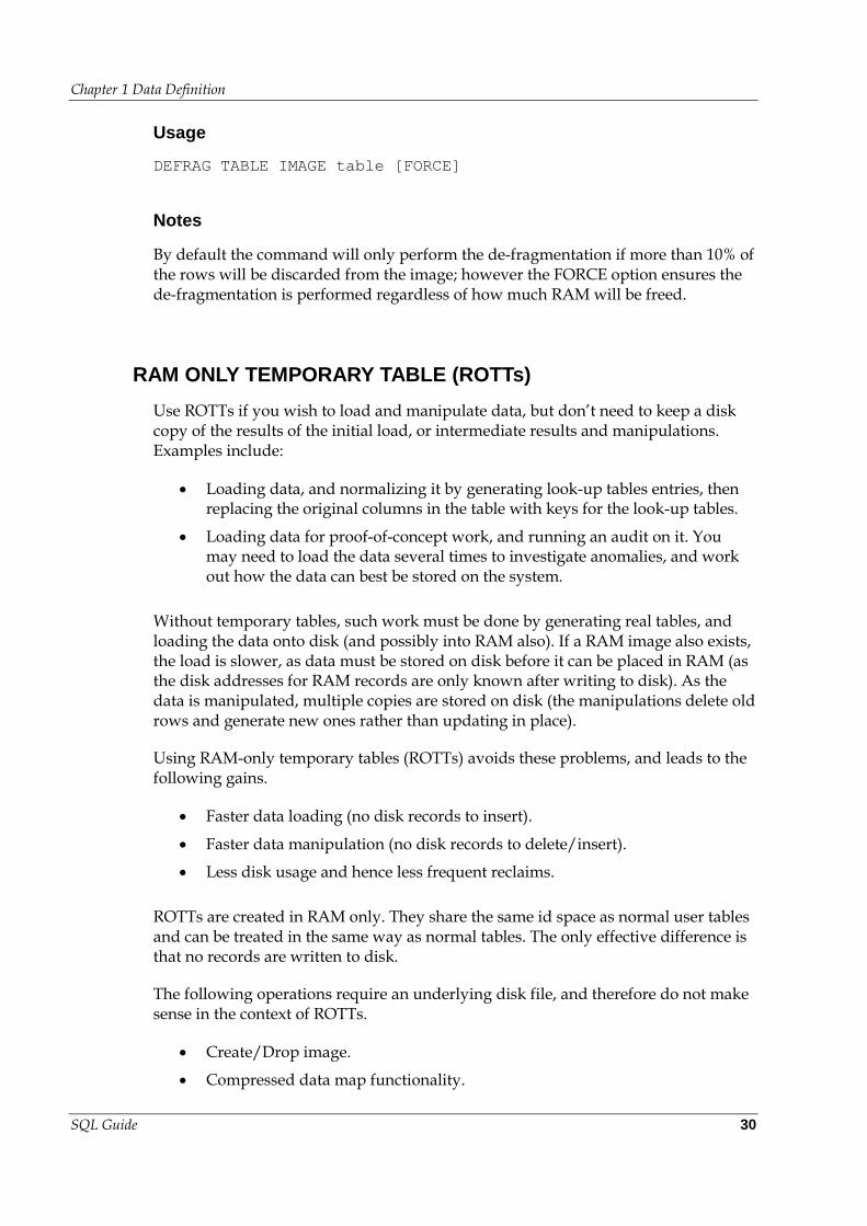
Chapter 1 Data Definition
SQL Guide 30
Usage
DEFRAG TABLE IMAGE table [FORCE]
Notes
By default the command will only perform the de-fragmentation if more than 10% of the rows will be discarded from the image; however the FORCE option ensures the de-fragmentation is performed regardless of how much RAM will be freed.
RAM ONLY TEMPORARY TABLE (ROTTs)
Use ROTTs if you wish to load and manipulate data, but don’t need to keep a disk copy of the results of the initial load, or intermediate results and manipulations. Examples include:
Loading data, and normalizing it by generating look-up tables entries, then replacing the original columns in the table with keys for the look-up tables.
Loading data for proof-of-concept work, and running an audit on it. You may need to load the data several times to investigate anomalies, and work out how the data can best be stored on the system.
Without temporary tables, such work must be done by generating real tables, and loading the data onto disk (and possibly into RAM also). If a RAM image also exists, the load is slower, as data must be stored on disk before it can be placed in RAM (as the disk addresses for RAM records are only known after writing to disk). As the data is manipulated, multiple copies are stored on disk (the manipulations delete old rows and generate new ones rather than updating in place).
Using RAM-only temporary tables (ROTTs) avoids these problems, and leads to the following gains.
Faster data loading (no disk records to insert).
Faster data manipulation (no disk records to delete/insert).
Less disk usage and hence less frequent reclaims.
ROTTs are created in RAM only. They share the same id space as normal user tables and can be treated in the same way as normal tables. The only effective difference is that no records are written to disk.
The following operations require an underlying disk file, and therefore do not make sense in the context of ROTTs.
Create/Drop image.
Compressed data map functionality.
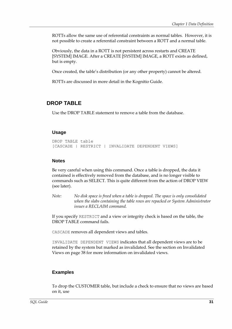
Chapter 1 Data Definition
SQL Guide 31
ROTTs allow the same use of referential constraints as normal tables. However, it is not possible to create a referential constraint between a ROTT and a normal table.
Obviously, the data in a ROTT is not persistent across restarts and CREATE [SYSTEM] IMAGE. After a CREATE [SYSTEM] IMAGE, a ROTT exists as defined, but is empty.
Once created, the table’s distribution (or any other property) cannot be altered.
ROTTs are discussed in more detail in the Kognitio Guide.
DROP TABLE
Use the DROP TABLE statement to remove a table from the database.
Usage
DROP TABLE table
[CASCADE | RESTRICT | INVALIDATE DEPENDENT VIEWS]
Notes
Be very careful when using this command. Once a table is dropped, the data it contained is effectively removed from the database, and is no longer visible to commands such as SELECT. This is quite different from the action of DROP VIEW (see later).
Note: No disk space is freed when a table is dropped. The space is only consolidated when the slabs containing the table rows are repacked or System Administrator issues a RECLAIM command.
If you specify RESTRICT and a view or integrity check is based on the table, the DROP TABLE command fails.
CASCADE removes all dependent views and tables.
INVALIDATE DEPENDENT VIEWS indicates that all dependent views are to be retained by the system but marked as invalidated. See the section on Invalidated Views on page 38 for more information on invalidated views.
Examples
To drop the CUSTOMER table, but include a check to ensure that no views are based on it, use
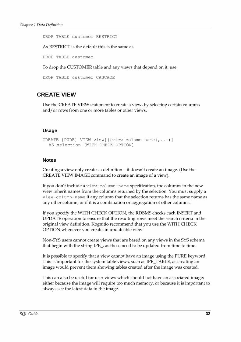
Chapter 1 Data Definition
SQL Guide 32
DROP TABLE customer RESTRICT
As RESTRICT is the default this is the same as
DROP TABLE customer
To drop the CUSTOMER table and any views that depend on it, use
DROP TABLE customer CASCADE
CREATE VIEW
Use the CREATE VIEW statement to create a view, by selecting certain columns and/or rows from one or more tables or other views.
Usage
CREATE [PURE] VIEW view[({view-column-name},...)]
AS selection [WITH CHECK OPTION]
Notes
Creating a view only creates a definition—it doesn’t create an image. (Use the CREATE VIEW IMAGE command to create an image of a view).
If you don’t include a view-column-name specification, the columns in the new view inherit names from the columns returned by the selection. You must supply a view-column-name if any column that the selection returns has the same name as any other column, or if it is a combination or aggregation of other columns.
If you specify the WITH CHECK OPTION, the RDBMS checks each INSERT and UPDATE operation to ensure that the resulting rows meet the search criteria in the original view definition. Kognitio recommend that you use the WITH CHECK OPTION whenever you create an updateable view.
Non-SYS users cannot create views that are based on any views in the SYS schema that begin with the string IPE_, as these need to be updated from time to time.
It is possible to specify that a view cannot have an image using the PURE keyword. This is important for the system table views, such as IPE_TABLE, as creating an image would prevent them showing tables created after the image was created.
This can also be useful for user views which should not have an associated image; either because the image will require too much memory, or because it is important to always see the latest data in the image.
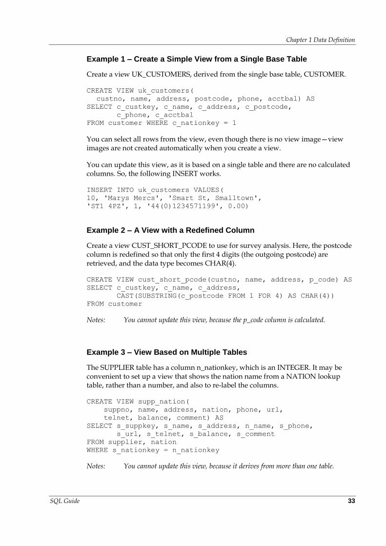
Chapter 1 Data Definition
SQL Guide 33
Example 1 – Create a Simple View from a Single Base Table
Create a view UK_CUSTOMERS, derived from the single base table, CUSTOMER.
CREATE VIEW uk_customers(
custno, name, address, postcode, phone, acctbal) AS
SELECT c_custkey, c_name, c_address, c_postcode,
c_phone, c_acctbal
FROM customer WHERE c_nationkey = 1
You can select all rows from the view, even though there is no view image—view images are not created automatically when you create a view.
You can update this view, as it is based on a single table and there are no calculated columns. So, the following INSERT works.
INSERT INTO uk_customers VALUES(
10, 'Marys Mercs', 'Smart St, Smalltown',
'ST1 4PZ', 1, '44(0)1234571199', 0.00)
Example 2 – A View with a Redefined Column
Create a view CUST_SHORT_PCODE to use for survey analysis. Here, the postcode column is redefined so that only the first 4 digits (the outgoing postcode) are retrieved, and the data type becomes CHAR(4).
CREATE VIEW cust_short_pcode(custno, name, address, p_code) AS
SELECT c_custkey, c_name, c_address,
CAST(SUBSTRING(c_postcode FROM 1 FOR 4) AS CHAR(4))
FROM customer
Notes: You cannot update this view, because the p_code column is calculated.
Example 3 – View Based on Multiple Tables
The SUPPLIER table has a column n_nationkey, which is an INTEGER. It may be convenient to set up a view that shows the nation name from a NATION lookup table, rather than a number, and also to re-label the columns.
CREATE VIEW supp_nation(
suppno, name, address, nation, phone, url,
telnet, balance, comment) AS
SELECT s_suppkey, s_name, s_address, n_name, s_phone,
s_url, s_telnet, s_balance, s_comment
FROM supplier, nation
WHERE s_nationkey = n_nationkey
Notes: You cannot update this view, because it derives from more than one table.
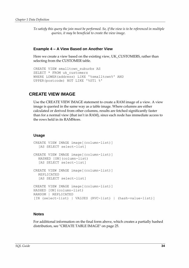
Chapter 1 Data Definition
SQL Guide 34
To satisfy this query the join must be performed. So, if the view is to be referenced in multiple queries, it may be beneficial to create the view image.
Example 4 – A View Based on Another View
Here we create a view based on the existing view, UK_CUSTOMERS, rather than selecting from the CUSTOMER table.
CREATE VIEW smalltown_suburbs AS
SELECT * FROM uk_customers
WHERE LOWER(address) LIKE '%smalltown%' AND
UPPER(postcode) NOT LIKE '%ST1 %'
CREATE VIEW IMAGE
Use the CREATE VIEW IMAGE statement to create a RAM image of a view. A view image is queried in the same way as a table image. Where columns are either calculated or derived from other columns, results are fetched significantly faster than for a normal view (that isn’t in RAM), since each node has immediate access to the rows held in its RAMStore.
Usage
CREATE VIEW IMAGE image[(column-list)]
[AS SELECT select-list]
CREATE VIEW IMAGE image[(column-list)]
HASHED [ON](column-list)
[AS SELECT select-list]
CREATE VIEW IMAGE image[(column-list)]
REPLICATED
[AS SELECT select-list]
CREATE VIEW IMAGE image[(column-list)]
HASHED [ON](column-list)
RANDOM | REPLICATED
[IN (select-list) | VALUES (RVC-list) | (hash-value-list)]
Notes
For additional information on the final form above, which creates a partially hashed distribution, see "CREATE TABLE IMAGE" on page 25.
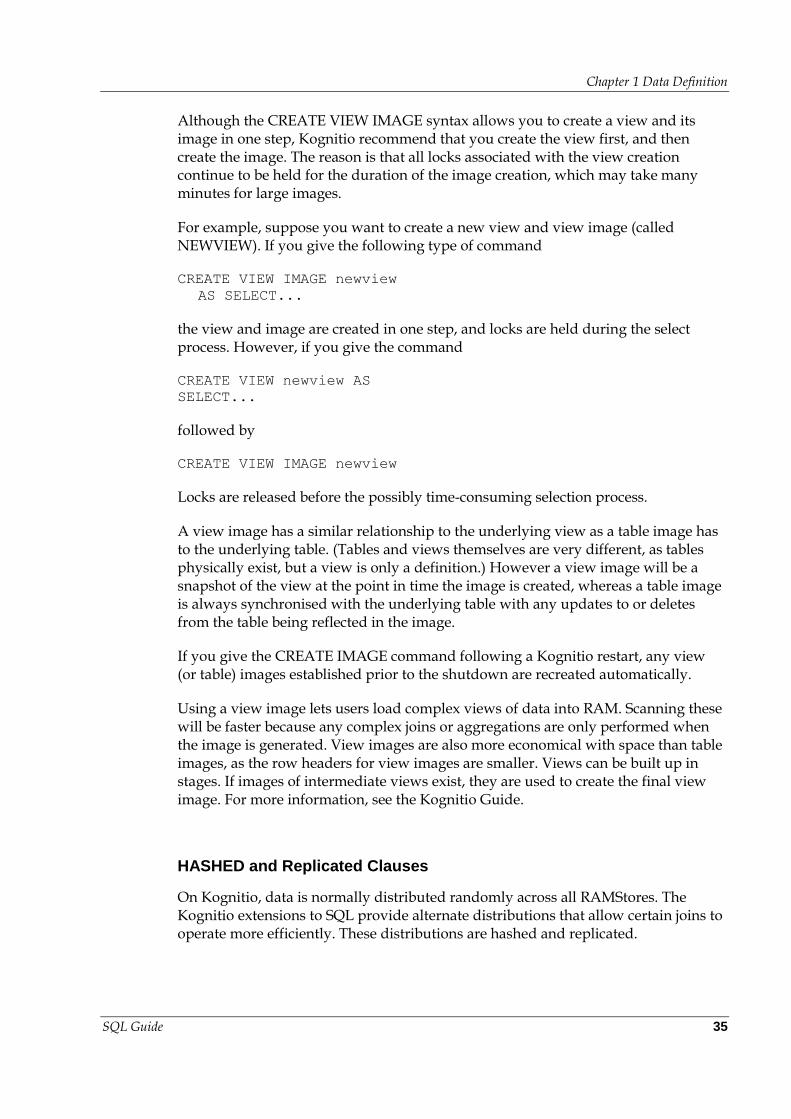
Chapter 1 Data Definition
SQL Guide 35
Although the CREATE VIEW IMAGE syntax allows you to create a view and its image in one step, Kognitio recommend that you create the view first, and then create the image. The reason is that all locks associated with the view creation continue to be held for the duration of the image creation, which may take many minutes for large images.
For example, suppose you want to create a new view and view image (called NEWVIEW). If you give the following type of command
CREATE VIEW IMAGE newview
AS SELECT...
the view and image are created in one step, and locks are held during the select process. However, if you give the command
CREATE VIEW newview AS
SELECT...
followed by
CREATE VIEW IMAGE newview
Locks are released before the possibly time-consuming selection process.
A view image has a similar relationship to the underlying view as a table image has to the underlying table. (Tables and views themselves are very different, as tables physically exist, but a view is only a definition.) However a view image will be a snapshot of the view at the point in time the image is created, whereas a table image is always synchronised with the underlying table with any updates to or deletes from the table being reflected in the image.
If you give the CREATE IMAGE command following a Kognitio restart, any view (or table) images established prior to the shutdown are recreated automatically.
Using a view image lets users load complex views of data into RAM. Scanning these will be faster because any complex joins or aggregations are only performed when the image is generated. View images are also more economical with space than table images, as the row headers for view images are smaller. Views can be built up in stages. If images of intermediate views exist, they are used to create the final view image. For more information, see the Kognitio Guide.
HASHED and Replicated Clauses
On Kognitio, data is normally distributed randomly across all RAMStores. The Kognitio extensions to SQL provide alternate distributions that allow certain joins to operate more efficiently. These distributions are hashed and replicated.
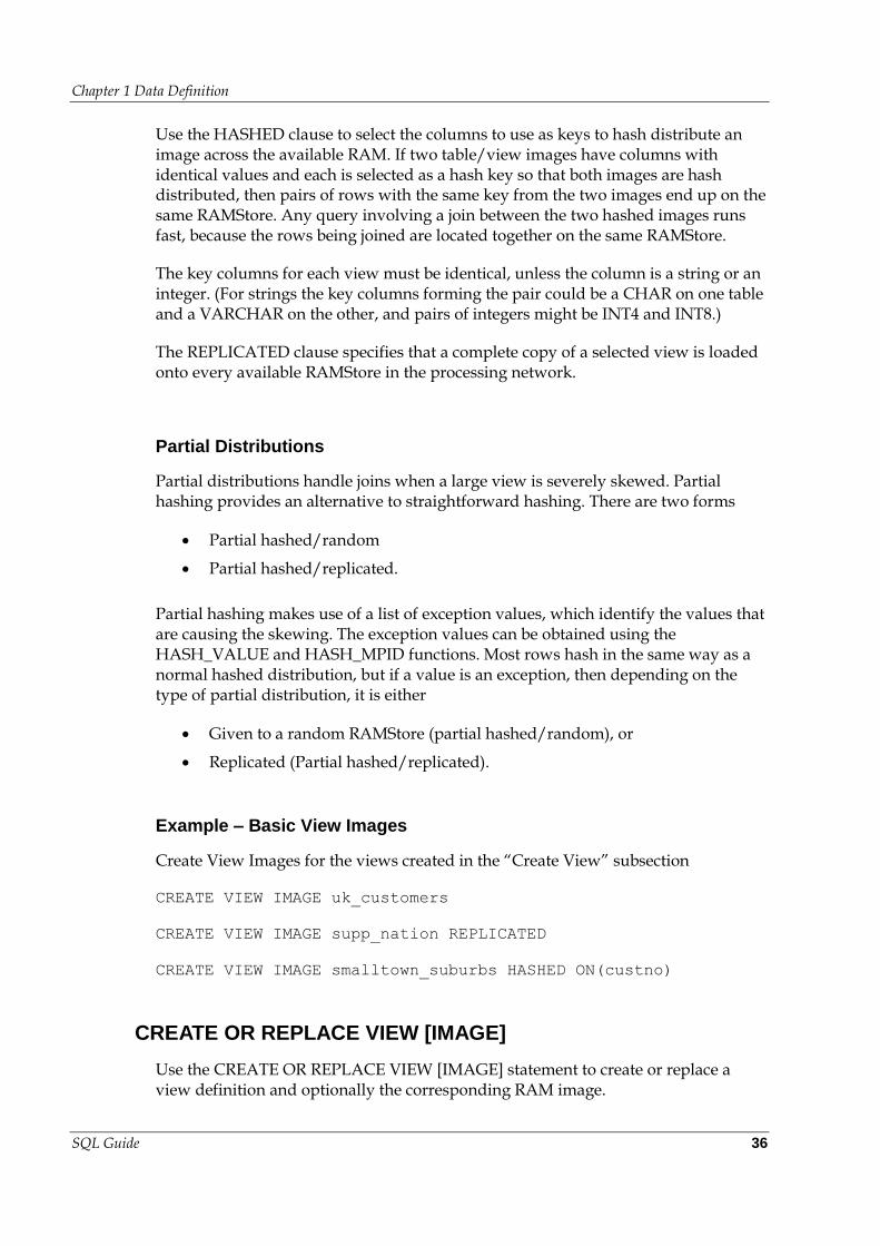
Chapter 1 Data Definition
SQL Guide 36
Use the HASHED clause to select the columns to use as keys to hash distribute an image across the available RAM. If two table/view images have columns with identical values and each is selected as a hash key so that both images are hash distributed, then pairs of rows with the same key from the two images end up on the same RAMStore. Any query involving a join between the two hashed images runs fast, because the rows being joined are located together on the same RAMStore.
The key columns for each view must be identical, unless the column is a string or an integer. (For strings the key columns forming the pair could be a CHAR on one table and a VARCHAR on the other, and pairs of integers might be INT4 and INT8.)
The REPLICATED clause specifies that a complete copy of a selected view is loaded onto every available RAMStore in the processing network.
Partial Distributions
Partial distributions handle joins when a large view is severely skewed. Partial hashing provides an alternative to straightforward hashing. There are two forms
Partial hashed/random
Partial hashed/replicated.
Partial hashing makes use of a list of exception values, which identify the values that are causing the skewing. The exception values can be obtained using the HASH_VALUE and HASH_MPID functions. Most rows hash in the same way as a normal hashed distribution, but if a value is an exception, then depending on the type of partial distribution, it is either
Given to a random RAMStore (partial hashed/random), or
Replicated (Partial hashed/replicated).
Example – Basic View Images
Create View Images for the views created in the “Create View” subsection
CREATE VIEW IMAGE uk_customers
CREATE VIEW IMAGE supp_nation REPLICATED
CREATE VIEW IMAGE smalltown_suburbs HASHED ON(custno)
CREATE OR REPLACE VIEW [IMAGE]
Use the CREATE OR REPLACE VIEW [IMAGE] statement to create or replace a view definition and optionally the corresponding RAM image.
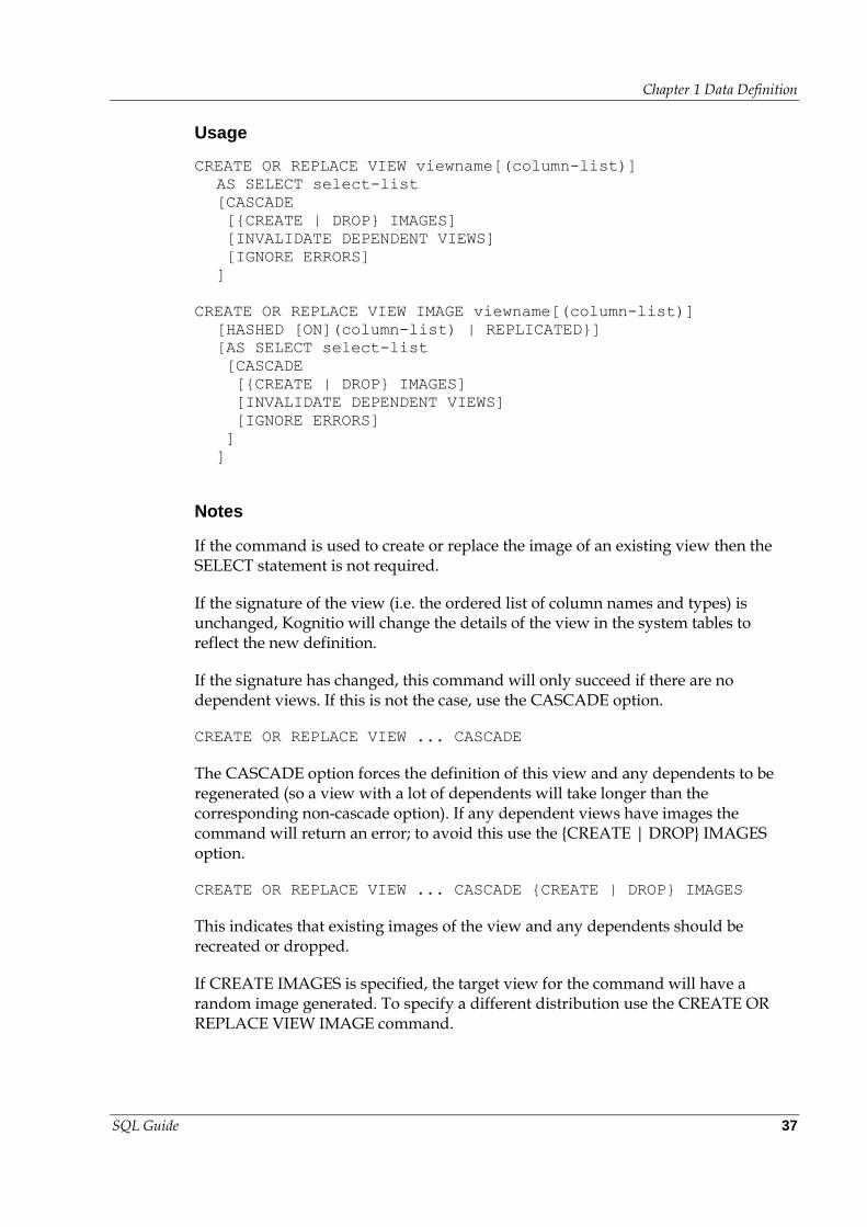
Chapter 1 Data Definition
SQL Guide 37
Usage
CREATE OR REPLACE VIEW viewname[(column-list)]
AS SELECT select-list
[CASCADE
[{CREATE | DROP} IMAGES]
[INVALIDATE DEPENDENT VIEWS]
[IGNORE ERRORS]
]
CREATE OR REPLACE VIEW IMAGE viewname[(column-list)]
[HASHED [ON](column-list) | REPLICATED}]
[AS SELECT select-list
[CASCADE
[{CREATE | DROP} IMAGES]
[INVALIDATE DEPENDENT VIEWS]
[IGNORE ERRORS]
]
]
Notes
If the command is used to create or replace the image of an existing view then the SELECT statement is not required.
If the signature of the view (i.e. the ordered list of column names and types) is unchanged, Kognitio will change the details of the view in the system tables to reflect the new definition.
If the signature has changed, this command will only succeed if there are no dependent views. If this is not the case, use the CASCADE option.
CREATE OR REPLACE VIEW ... CASCADE
The CASCADE option forces the definition of this view and any dependents to be regenerated (so a view with a lot of dependents will take longer than the corresponding non-cascade option). If any dependent views have images the command will return an error; to avoid this use the {CREATE | DROP} IMAGES option.
CREATE OR REPLACE VIEW ... CASCADE {CREATE | DROP} IMAGES
This indicates that existing images of the view and any dependents should be recreated or dropped.
If CREATE IMAGES is specified, the target view for the command will have a random image generated. To specify a different distribution use the CREATE OR REPLACE VIEW IMAGE command.
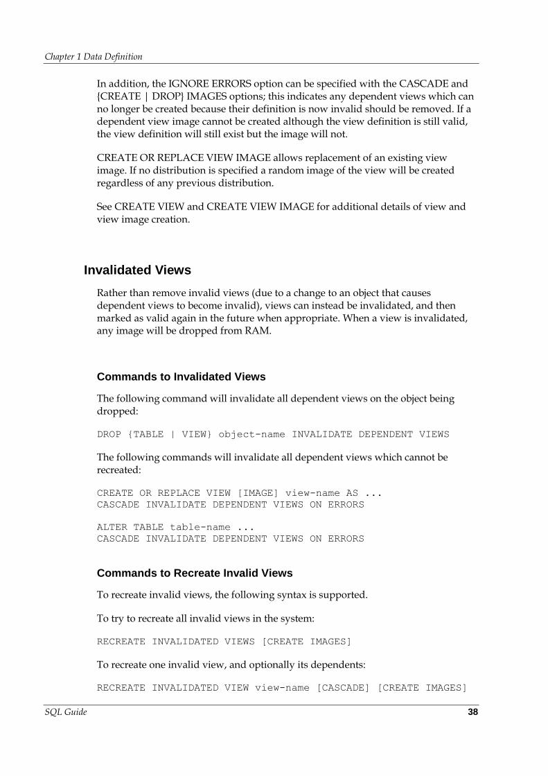
Chapter 1 Data Definition
SQL Guide 38
In addition, the IGNORE ERRORS option can be specified with the CASCADE and {CREATE | DROP} IMAGES options; this indicates any dependent views which can no longer be created because their definition is now invalid should be removed. If a dependent view image cannot be created although the view definition is still valid, the view definition will still exist but the image will not.
CREATE OR REPLACE VIEW IMAGE allows replacement of an existing view image. If no distribution is specified a random image of the view will be created regardless of any previous distribution.
See CREATE VIEW and CREATE VIEW IMAGE for additional details of view and view image creation.
Invalidated Views
Rather than remove invalid views (due to a change to an object that causes dependent views to become invalid), views can instead be invalidated, and then marked as valid again in the future when appropriate. When a view is invalidated, any image will be dropped from RAM.
Commands to Invalidated Views
The following command will invalidate all dependent views on the object being dropped:
DROP {TABLE | VIEW} object-name INVALIDATE DEPENDENT VIEWS
The following commands will invalidate all dependent views which cannot be recreated:
CREATE OR REPLACE VIEW [IMAGE] view-name AS ...
CASCADE INVALIDATE DEPENDENT VIEWS ON ERRORS
ALTER TABLE table-name ...
CASCADE INVALIDATE DEPENDENT VIEWS ON ERRORS
Commands to Recreate Invalid Views
To recreate invalid views, the following syntax is supported.
To try to recreate all invalid views in the system:
RECREATE INVALIDATED VIEWS [CREATE IMAGES]
To recreate one invalid view, and optionally its dependents:
RECREATE INVALIDATED VIEW view-name [CASCADE] [CREATE IMAGES]
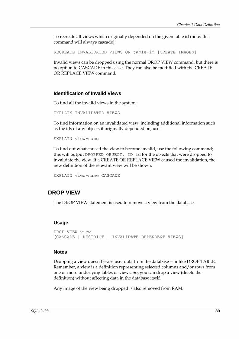
Chapter 1 Data Definition
SQL Guide 39
To recreate all views which originally depended on the given table id (note: this command will always cascade):
RECREATE INVALIDATED VIEWS ON table-id [CREATE IMAGES]
Invalid views can be dropped using the normal DROP VIEW command, but there is no option to CASCADE in this case. They can also be modified with the CREATE OR REPLACE VIEW command.
Identification of Invalid Views
To find all the invalid views in the system:
EXPLAIN INVALIDATED VIEWS
To find information on an invalidated view, including additional information such as the ids of any objects it originally depended on, use:
EXPLAIN view-name
To find out what caused the view to become invalid, use the following command; this will output DROPPED OBJECT, ID id for the objects that were dropped to invalidate the view. If a CREATE OR REPLACE VIEW caused the invalidation, the new definition of the relevant view will be shown:
EXPLAIN view-name CASCADE
DROP VIEW
The DROP VIEW statement is used to remove a view from the database.
Usage
DROP VIEW view
[CASCADE | RESTRICT | INVALIDATE DEPENDENT VIEWS]
Notes
Dropping a view doesn’t erase user data from the database—unlike DROP TABLE. Remember, a view is a definition representing selected columns and/or rows from one or more underlying tables or views. So, you can drop a view (delete the definition) without affecting data in the database itself.
Any image of the view being dropped is also removed from RAM.
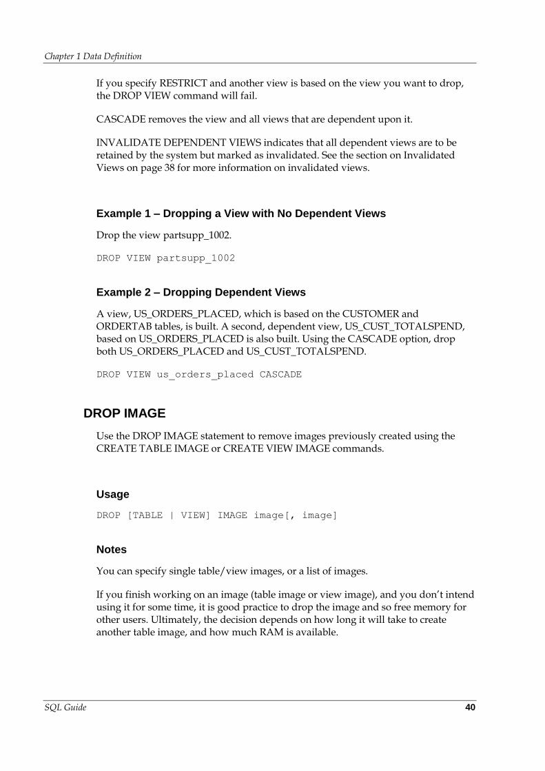
Chapter 1 Data Definition
SQL Guide 40
If you specify RESTRICT and another view is based on the view you want to drop, the DROP VIEW command will fail.
CASCADE removes the view and all views that are dependent upon it.
INVALIDATE DEPENDENT VIEWS indicates that all dependent views are to be retained by the system but marked as invalidated. See the section on Invalidated Views on page 38 for more information on invalidated views.
Example 1 – Dropping a View with No Dependent Views
Drop the view partsupp_1002.
DROP VIEW partsupp_1002
Example 2 – Dropping Dependent Views
A view, US_ORDERS_PLACED, which is based on the CUSTOMER and ORDERTAB tables, is built. A second, dependent view, US_CUST_TOTALSPEND, based on US_ORDERS_PLACED is also built. Using the CASCADE option, drop both US_ORDERS_PLACED and US_CUST_TOTALSPEND.
DROP VIEW us_orders_placed CASCADE
DROP IMAGE
Use the DROP IMAGE statement to remove images previously created using the CREATE TABLE IMAGE or CREATE VIEW IMAGE commands.
Usage
DROP [TABLE | VIEW] IMAGE image[, image]
Notes
You can specify single table/view images, or a list of images.
If you finish working on an image (table image or view image), and you don’t intend using it for some time, it is good practice to drop the image and so free memory for other users. Ultimately, the decision depends on how long it will take to create another table image, and how much RAM is available.
Chapter 1 Data Definition
SQL Guide 41
Example
To drop the images of the PART and PARTSUPP tables, use
DROP TABLE IMAGE part, partsupp
Alternately, you could use
DROP IMAGE part, partsupp
Annotating Objects with Comments
It is possible to annotate objects with comments using the ALTER statement.
Usage
ALTER {SCHEMA | TABLE | VIEW} object-name
SET COMMENT TO 'string'
ALTER {TABLE | VIEW} object-name ALTER COLUMN column-name
SET COMMENT TO 'string'
Notes
Comments will be displayed for objects if the EXPLAIN command is prefixed to the object; comments can also be viewed in the SYS.IPE_COMMENT view.
In addition, the SYS.IPE_DESCRIPTION view can be used to look up information on a particular subject. For example:
SELECT * FROM SYS.IPE_DESCRIPTION WHERE COMMENT IMATCHING
'privilege' ORDER BY 1,2,3
Comments for an object can be removed by setting them to the empty string.
There is a comment privilege which users need to be granted in order to be able to set comments on an object.

Kognitio SQL Guide 43
2
Data Manipulation
This chapter gives details of the SQL statements and commands that can be used to manipulate data in a database.
2.1 SELECT Statement
Use the SELECT statement to retrieve data from a database, and return it in the form of a table of query results.
Usage
[[SELECT] WITH vname AS (select-statement) [,vname AS...]]
SELECT [TOP row-count] [ALL | DISTINCT] {* | select-list}
FROM {{{table | view
[{TABLESAMPLE [method] (percentage) [REPEATABLE (arg)]}]} |
joined-table | derived-table | literal } [correlation]},...
[WHERE search-condition]
[GROUP BY {column-name | column-number |
GROUPING SETS (column-list),...}]
[HAVING search-condition]
[ORDER BY {{column-name | column-number}
[ASC | DESC] [NULLS {FIRST | LAST | MAX | MIN}],...}]
[AT {NOW | FULL_HISTORY}]
[FETCH FIRST row-count ROWS ONLY]
Chapter 2 Data Manipulation
SQL Guide 44
Notes
AT NOW is a Kognitio extension to SQL that shows the current state of a table excluding any currently active transactions that might be altering the contents. AT FULL_HISTORY is primarily for use by the archiving mechanism as it shows all the records in a table—including those that have been updated.
The WITH Clause
The WITH clause allows “views” to be temporarily created on a per-query basis. If the vname is the same as an existing table or view, it takes priority over the existing object. WITH clauses cannot be nested but they can refer to previously defined WITH clauses.
WITH Clauses are very similar to derived tables which are discussed in this manual and the Kognitio Guide.
The following example uses a WITH clause to simplify a query to count the total number of line items excluding the group of line items that occur most infrequently:
SELECT WITH
-- lncnt counts the occurrences per linenumber
lncnt(ln, c) AS (
SELECT l_linenumber, COUNT(l_orderkey)
FROM lineitem GROUP BY 1),
-- lnmin determines the line number that occurs least
lnmin(mn) AS (
SELECT ln
FROM lncnt
WHERE c IN (SELECT MIN(c) FROM lncnt))
-- Now return the count of line numbers excluding the minimum
SELECT COUNT(l_linenumber)
FROM lineitem, lnmin
WHERE l_linenumber NOT IN (mn);
The SELECT Clause
The select clause specifies which columns to include. The asterisk (*) specifies "all columns". If you don’t use the asterisk, you must give the names of the columns to include.
TOP row-count defines the maximum number of rows that are to be returned. The default is to return all rows. Use ORDER BY to specify the sequence the rows are returned. It is also possible to specify the maximum number of rows to be returned by using the FETCH FIRST row-count ROWS ONLY clause.
DISTINCT is a keyword that means, where identical rows exist, only one row is returned. The default is ALL.
Chapter 2 Data Manipulation
SQL Guide 45
Columns are returned in the order in which they are specified in the SELECT clause. If the asterisk is used then the columns are returned in the order that they are defined in the underlying table or tables.
The FROM Clause
The FROM clause specifies the table(s) or view(s) to select rows from.
FROM
{{{table | view
[{TABLESAMPLE [method] (percentage) [REPEATABLE (arg)]}]} |
joined-table | derived-table | literal}
[correlation]},...
A derived table is a SQL construct consisting of a SELECT statement embedded in the FROM clause of another SELECT statement. Derived table support is required for full ANSI-92 SQL compliance. Derived tables are referred to by a variety of names, including: table subqueries, nested queries, and table value constructors (the formal ANSI-92 SQL name).
Derived tables let you develop queries in a modular way. This means that using them is quite similar to using views and view images, but there are obvious advantages for one-off queries. They can also remove duplication and make queries easier to read. Derived tables are discussed in detail in the Kognitio Guide. There are also various examples in this manual.
It is also possible to use literal values instead of a table or view. For example:
SELECT 2 * pi() * r AS circumference
FROM (VALUES (100), (200), (400)) AS radius(r)
The FROM clause can be completely omitted if the SELECT statement is a constant expression. For example:
SELECT 2 * pi() * 100 AS circumference
The TABLESAMPLE [method] (percentage) [REPEATABLE(arg)] clause causes a sample of the table's contents to be selected. The method can be either the default SYSTEM, or BERNOULLI, the percentage is a value between 0 and 100 indicating the size of the sample that should be returned and the REPEATABLE(arg) is a positive integer that will ensure repeatability of the results by being used as the random seed that is used to identify the table sample, (i.e. if you use the same argument on the same table you will get the same sample); if arg is zero or omitted then the sample returned will be random.
Note: The BERNOULLI method was implemented because it is part of the SQL standard; however using the BERNOULLI method is likely to be slow due to the requirement to handle identical rows independently.
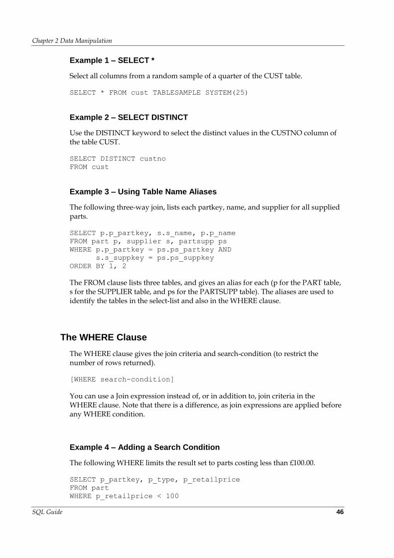
Chapter 2 Data Manipulation
SQL Guide 46
Example 1 – SELECT *
Select all columns from a random sample of a quarter of the CUST table.
SELECT * FROM cust TABLESAMPLE SYSTEM(25)
Example 2 – SELECT DISTINCT
Use the DISTINCT keyword to select the distinct values in the CUSTNO column of the table CUST.
SELECT DISTINCT custno
FROM cust
Example 3 – Using Table Name Aliases
The following three-way join, lists each partkey, name, and supplier for all supplied parts.
SELECT p.p_partkey, s.s_name, p.p_name
FROM part p, supplier s, partsupp ps
WHERE p.p_partkey = ps.ps_partkey AND
s.s_suppkey = ps.ps_suppkey
ORDER BY 1, 2
The FROM clause lists three tables, and gives an alias for each (p for the PART table, s for the SUPPLIER table, and ps for the PARTSUPP table). The aliases are used to identify the tables in the select-list and also in the WHERE clause.
The WHERE Clause
The WHERE clause gives the join criteria and search-condition (to restrict the number of rows returned).
[WHERE search-condition]
You can use a Join expression instead of, or in addition to, join criteria in the WHERE clause. Note that there is a difference, as join expressions are applied before any WHERE condition.
Example 4 – Adding a Search Condition
The following WHERE limits the result set to parts costing less than £100.00.
SELECT p_partkey, p_type, p_retailprice
FROM part
WHERE p_retailprice < 100
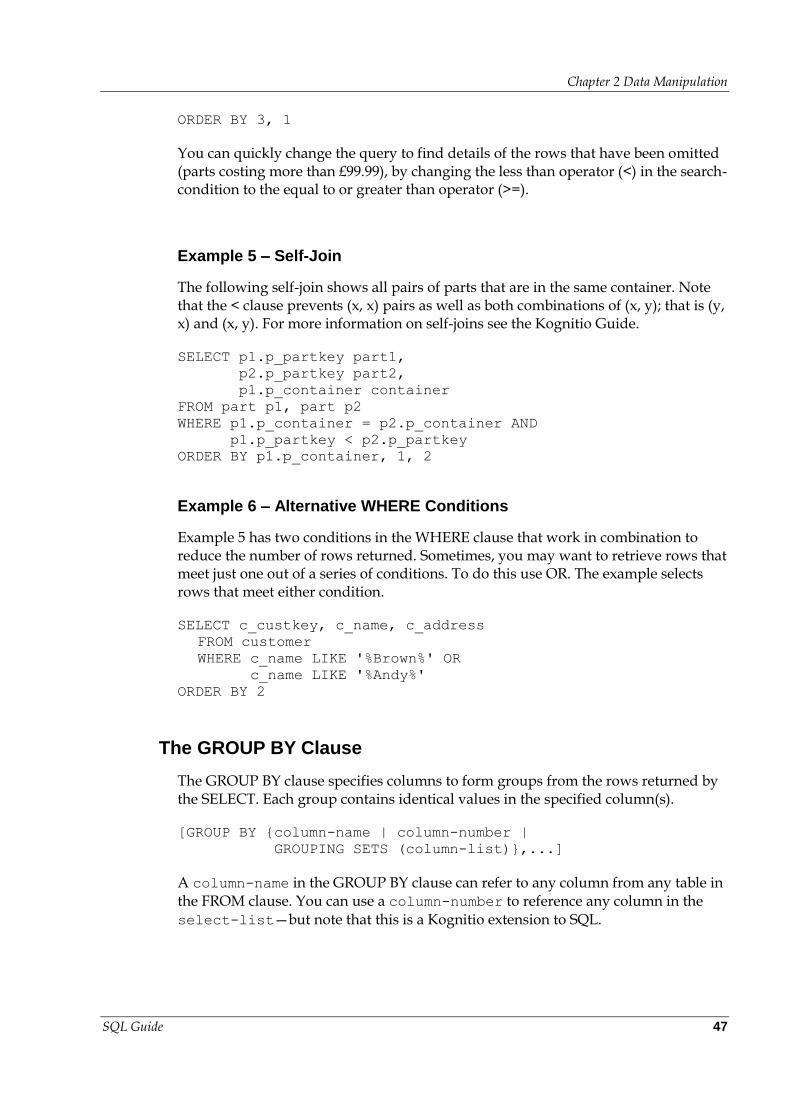
Chapter 2 Data Manipulation
SQL Guide 47
ORDER BY 3, 1
You can quickly change the query to find details of the rows that have been omitted (parts costing more than £99.99), by changing the less than operator (<) in the search-condition to the equal to or greater than operator (>=).
Example 5 – Self-Join
The following self-join shows all pairs of parts that are in the same container. Note that the < clause prevents (x, x) pairs as well as both combinations of (x, y); that is (y, x) and (x, y). For more information on self-joins see the Kognitio Guide.
SELECT p1.p_partkey part1,
p2.p_partkey part2,
p1.p_container container
FROM part p1, part p2
WHERE p1.p_container = p2.p_container AND
p1.p_partkey < p2.p_partkey
ORDER BY p1.p_container, 1, 2
Example 6 – Alternative WHERE Conditions
Example 5 has two conditions in the WHERE clause that work in combination to reduce the number of rows returned. Sometimes, you may want to retrieve rows that meet just one out of a series of conditions. To do this use OR. The example selects rows that meet either condition.
SELECT c_custkey, c_name, c_address
FROM customer
WHERE c_name LIKE '%Brown%' OR
c_name LIKE '%Andy%'
ORDER BY 2
The GROUP BY Clause
The GROUP BY clause specifies columns to form groups from the rows returned by the SELECT. Each group contains identical values in the specified column(s).
[GROUP BY {column-name | column-number |
GROUPING SETS (column-list)},...]
A column-name in the GROUP BY clause can refer to any column from any table in the FROM clause. You can use a column-number to reference any column in the select-list—but note that this is a Kognitio extension to SQL.
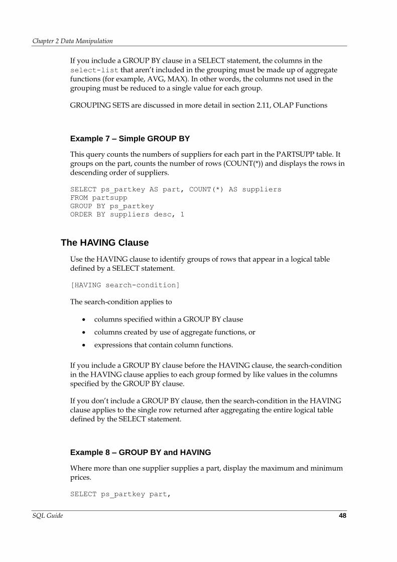
Chapter 2 Data Manipulation
SQL Guide 48
If you include a GROUP BY clause in a SELECT statement, the columns in the select-list that aren’t included in the grouping must be made up of aggregate functions (for example, AVG, MAX). In other words, the columns not used in the grouping must be reduced to a single value for each group.
GROUPING SETS are discussed in more detail in section 2.11, OLAP Functions
Example 7 – Simple GROUP BY
This query counts the numbers of suppliers for each part in the PARTSUPP table. It groups on the part, counts the number of rows (COUNT(*)) and displays the rows in descending order of suppliers.
SELECT ps_partkey AS part, COUNT(*) AS suppliers
FROM partsupp
GROUP BY ps_partkey
ORDER BY suppliers desc, 1
The HAVING Clause
Use the HAVING clause to identify groups of rows that appear in a logical table defined by a SELECT statement.
[HAVING search-condition]
The search-condition applies to
columns specified within a GROUP BY clause
columns created by use of aggregate functions, or
expressions that contain column functions.
If you include a GROUP BY clause before the HAVING clause, the search-condition in the HAVING clause applies to each group formed by like values in the columns specified by the GROUP BY clause.
If you don’t include a GROUP BY clause, then the search-condition in the HAVING clause applies to the single row returned after aggregating the entire logical table defined by the SELECT statement.
Example 8 – GROUP BY and HAVING
Where more than one supplier supplies a part, display the maximum and minimum prices.
SELECT ps_partkey part,
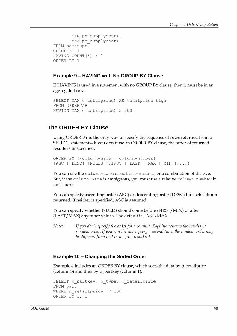
Chapter 2 Data Manipulation
SQL Guide 49
MIN(ps_supplycost),
MAX(ps_supplycost)
FROM partsupp
GROUP BY 1
HAVING COUNT(*) > 1
ORDER BY 1
Example 9 – HAVING with No GROUP BY Clause
If HAVING is used in a statement with no GROUP BY clause, then it must be in an aggregated row.
SELECT MAX(o_totalprice) AS totalprice_high
FROM ORDERTAB
HAVING MAX(o_totalprice) > 200
The ORDER BY Clause
Using ORDER BY is the only way to specify the sequence of rows returned from a SELECT statement—if you don’t use an ORDER BY clause, the order of returned results is unspecified.
ORDER BY {{column-name | column-number}
[ASC | DESC] [NULLS {FIRST | LAST | MAX | MIN}],...}
You can use the column-name or column-number, or a combination of the two. But, if the column-name is ambiguous, you must use a relative column-number in the clause.
You can specify ascending order (ASC) or descending order (DESC) for each column returned. If neither is specified, ASC is assumed.
You can specify whether NULLS should come before (FIRST/MIN) or after (LAST/MAX) any other values. The default is LAST/MAX.
Note: If you don’t specify the order for a column, Kognitio returns the results in random order. If you run the same query a second time, the random order may be different from that in the first result set.
Example 10 – Changing the Sorted Order
Example 4 includes an ORDER BY clause, which sorts the data by p_retailprice (column 3) and then by p_partkey (column 1).
SELECT p_partkey, p_type, p_retailprice
FROM part
WHERE p_retailprice < 100
ORDER BY 3, 1
Chapter 2 Data Manipulation
SQL Guide 50
If you change the ORDER BY clause to
ORDER BY p_retailprice, p_partkey
You get the same result, because you are just using column names instead of numbers.
If you changed the ORDER BY clause to
ORDER BY p_partkey, p_retailprice
Then you would first sort by p_partkey and then p_retailprice. Since p_partkey is unique, you would never actually sort by price, note that this is not the same as the earlier example where several parts may have the same price, which would then be sorted by part number.
Example 11 – Sorting in Descending Order
So far, the majority of result sets have been sorted in ascending order (lower through higher), which is the default. You can also specify descending order (higher through lower) for any column. The statement below sorts the results by p_retailprice in descending order, but any parts with the same value are sorted on p_partkey in ascending order. We also ensure that any p_retailprice values that are NULL are returned first.
ORDER BY p_retailprice DESC NULLS FIRST, p_partkey
2.2 INSERT
Use the INSERT statement to insert one or more rows into the specified table or view.
Use the VALUES clause to specify explicit values to insert. To insert rows from another table or view, include a SELECT statement—the number of rows inserted equals the number returned by the SELECT.
Usage
Inserting explicit values
INSERT INTO {table | view}[(column-list)]
VALUES(insert-list) [,...]
Insert-Select
INSERT INTO {table | view}[(column-list)] SELECT...
Chapter 2 Data Manipulation
SQL Guide 51
Notes
The SELECT statement can be any normal SELECT.
It is possible to provide some ordering on an insert-select operation which should improve the efficiency of any compressed indices built on the target table. Adding an ORDER BY to the INSERT-SELECT or CREATE TABLE AS statement will cause individual nodes to order results before writing to disk. So data from a process will be ordered before writing to disk, but this will be interleaved with ordered data from all other processes, hence the ordering is referred to as partial ordering.
If you use a view as the target of the insert, it must be formed from a single base table and cannot be read-only. You cannot insert into a view created using a UNION operator.
If you insert into a view created using the WITH CHECK OPTION, the inserted row must pass the table or view selection criteria (see Example 5).
Example 1 – Inserting Explicit Values (INSERT VALUES)
Insert values into table PARTSUPP_1, this table has the following creation statement:
CREATE TABLE partsupp_1(
ps_partkey INT NOT NULL,
ps_suppkey INT NOT NULL,
ps_availqty INTEGER NOT NULL,
ps_supplycost DECIMAL(12, 2) NOT NULL,
ps_comment VARCHAR(199) NOT NULL,
PRIMARY KEY(ps_partkey, ps_suppkey))
Now insert some data
INSERT INTO partsupp_1 VALUES(1, 1001, 10, 10.00, ''),
(2, 1001, 15, 40.00, ''), (3, 1001, 20, 20.00, ''),
INSERT INTO partsupp_1(ps_partkey, ps_suppkey, ps_availqty,
ps_supplycost, ps_comment )
VALUES(2, 1001, 15, 40.00, '')
Note: The column-list used here is optional.
Example 2 – INSERT-SELECT
In this example a second table, PARTSUPP_2, with the same column definitions as PARTSUPP_1 is created and the contents of the PARTSUPP_1 table inserted.
INSERT INTO partsupp_2
SELECT * FROM partsupp_1
Chapter 2 Data Manipulation
SQL Guide 52
You can use a WHERE condition to add a subset of rows from a table or view. So, the following statement
INSERT INTO partsupp_2
SELECT * FROM partsupp_1
WHERE ps_availqty = 10
only adds the rows where ps_availqty is 10.
Example 3 – Insert Using a Column-List
You can retrieve a subset of columns from one table, in this case PARTSUPP_1, and insert them into a second table with columns of the same type but different names. The CREATE statement of the new table is given below.
CREATE TABLE partsupp_3(
partkey INT NOT NULL,
suppkey INT NOT NULL,
availqty INTEGER NOT NULL,
supplycost DECIMAL(12, 2) NOT NULL
)
INSERT INTO partsupp_3(
partkey, availqty, suppkey, supplycost )
SELECT ps_partkey, ps_availqty,ps_suppkey, ps_supplycost
FROM partsupp_1
WHERE PS_SUPPLYCOST = 100
Example 4 – Inserting Rows from a Table with Fewer Columns
You can insert rows into one table from a second table with fewer columns, by using a column-list to identify which columns the data applies to.
If a column that isn’t in the column-list was defined with a default value, then the default value appears in each new row that is added. If there is no default value for an unspecified column, NULL is inserted.
To see this, another table, PARTSUPP_4 is created, with a default value in the ps_comment field instead of NOT NULL. Note that none of the columns here include the NOT NULL keywords.
CREATE TABLE partsupp_4(
ps_partkey INT,
ps_suppkey INT,
ps_availqty INTEGER,
ps_supplycost Decimal(12, 2),
ps_comment VARCHAR(199) DEFAULT ‘no comment’ )
INSERT INTO partsupp_4(ps_partkey, ps_availqty, ps_suppkey)
SELECT partkey, availqty, suppkey
Chapter 2 Data Manipulation
SQL Guide 53
FROM partsupp_3
The ps_comment column is filled with the default value, “no comment” as there is no comment column selected from partsupp_3.
The ps_supplycost column, which is also absent from the selection list but doesn’t have a default value, is filled with NULLs.
If you had tried to use this INSERT statement to add this data into the PARTSUPP_3 table, you would have received the error
“Attempt to NULL a non-NULL field”,
Because the unspecified columns in partsupp_3 are defined to be NOT NULL.
Example 5 – Inserting into a Table Created using a Check Constraint
Table PARTSUPP_5 is created with a check constraint to ensure that values entered into it are above 100.
CREATE TABLE partsupp_5(
partkey INT NOT NULL, CHECK(partkey > 100),
suppkey INT NOT NULL,
availqty INTEGER NOT NULL,
supplycost DECIMAL(12, 2) NOT NULL
)
If you attempt to insert the following INSERT statement
INSERT INTO partsupp_5 VALUES(9, 1001, 10, 5.00)
You receive the error message
“CI8045: Check Constraint Violation”,
Because the value for ps_partkey (9) is below 100. Inserting the following statement, where the value for ps_partkey is over 100, succeeds.
INSERT INTO partsupp_5 VALUES(109, 1001, 10, 5.00)
Example 6 – Inserting into a View
You can insert into a view formed from a single base table that isn’t read only.
Suppose you create a view, PARTSUPP_1002, which only containing records where ps_suppkey = 1002 using the following CREATE VIEW statement.
CREATE VIEW partsupp_1002 AS
SELECT *
FROM partsupp
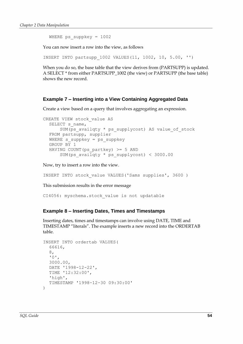
Chapter 2 Data Manipulation
SQL Guide 54
WHERE ps_suppkey = 1002
You can now insert a row into the view, as follows
INSERT INTO partsupp_1002 VALUES(11, 1002, 10, 5.00, '')
When you do so, the base table that the view derives from (PARTSUPP) is updated. A SELECT * from either PARTSUPP_1002 (the view) or PARTSUPP (the base table) shows the new record.
Example 7 – Inserting into a View Containing Aggregated Data
Create a view based on a query that involves aggregating an expression.
CREATE VIEW stock_value AS
SELECT s_name,
SUM(ps_availqty * ps_supplycost) AS value_of_stock
FROM partsupp, supplier
WHERE s_suppkey = ps_suppkey
GROUP BY 1
HAVING COUNT(ps_partkey) >= 5 AND
SUM(ps_availqty * ps_supplycost) < 3000.00
Now, try to insert a row into the view.
INSERT INTO stock_value VALUES('Sams supplies', 3600 )
This submission results in the error message
CI4056: myschema.stock_value is not updatable
Example 8 – Inserting Dates, Times and Timestamps
Inserting dates, times and timestamps can involve using DATE, TIME and TIMESTAMP “literals”. The example inserts a new record into the ORDERTAB table.
INSERT INTO ordertab VALUES(
66616,
8,
'0',
3000.00,
DATE '1998-12-22',
TIME '12:32:00',
'high',
TIMESTAMP '1998-12-30 09:30:00'
)
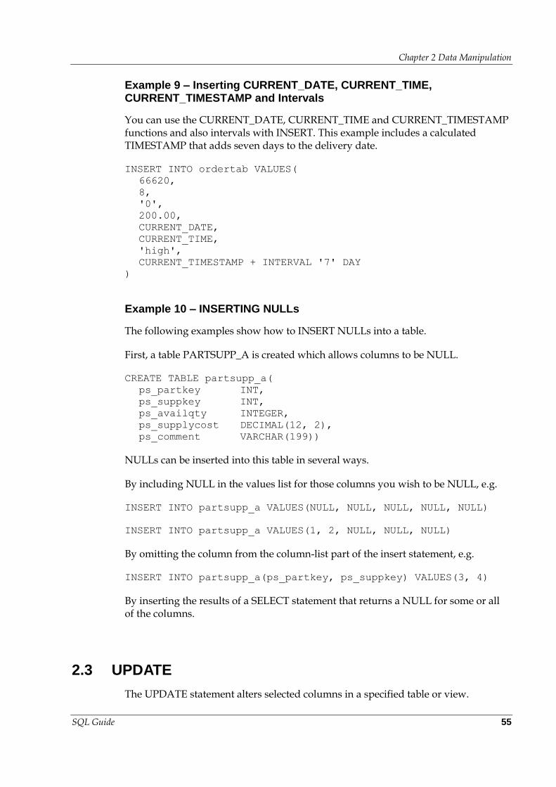
Chapter 2 Data Manipulation
SQL Guide 55
Example 9 – Inserting CURRENT_DATE, CURRENT_TIME, CURRENT_TIMESTAMP and Intervals
You can use the CURRENT_DATE, CURRENT_TIME and CURRENT_TIMESTAMP functions and also intervals with INSERT. This example includes a calculated TIMESTAMP that adds seven days to the delivery date.
INSERT INTO ordertab VALUES(
66620,
8,
'0',
200.00,
CURRENT_DATE,
CURRENT_TIME,
'high',
CURRENT_TIMESTAMP + INTERVAL '7' DAY
)
Example 10 – INSERTING NULLs
The following examples show how to INSERT NULLs into a table.
First, a table PARTSUPP_A is created which allows columns to be NULL.
CREATE TABLE partsupp_a(
ps_partkey INT,
ps_suppkey INT,
ps_availqty INTEGER,
ps_supplycost DECIMAL(12, 2),
ps_comment VARCHAR(199))
NULLs can be inserted into this table in several ways.
By including NULL in the values list for those columns you wish to be NULL, e.g.
INSERT INTO partsupp_a VALUES(NULL, NULL, NULL, NULL, NULL)
INSERT INTO partsupp_a VALUES(1, 2, NULL, NULL, NULL)
By omitting the column from the column-list part of the insert statement, e.g.
INSERT INTO partsupp_a(ps_partkey, ps_suppkey) VALUES(3, 4)
By inserting the results of a SELECT statement that returns a NULL for some or all of the columns.
2.3 UPDATE
The UPDATE statement alters selected columns in a specified table or view.
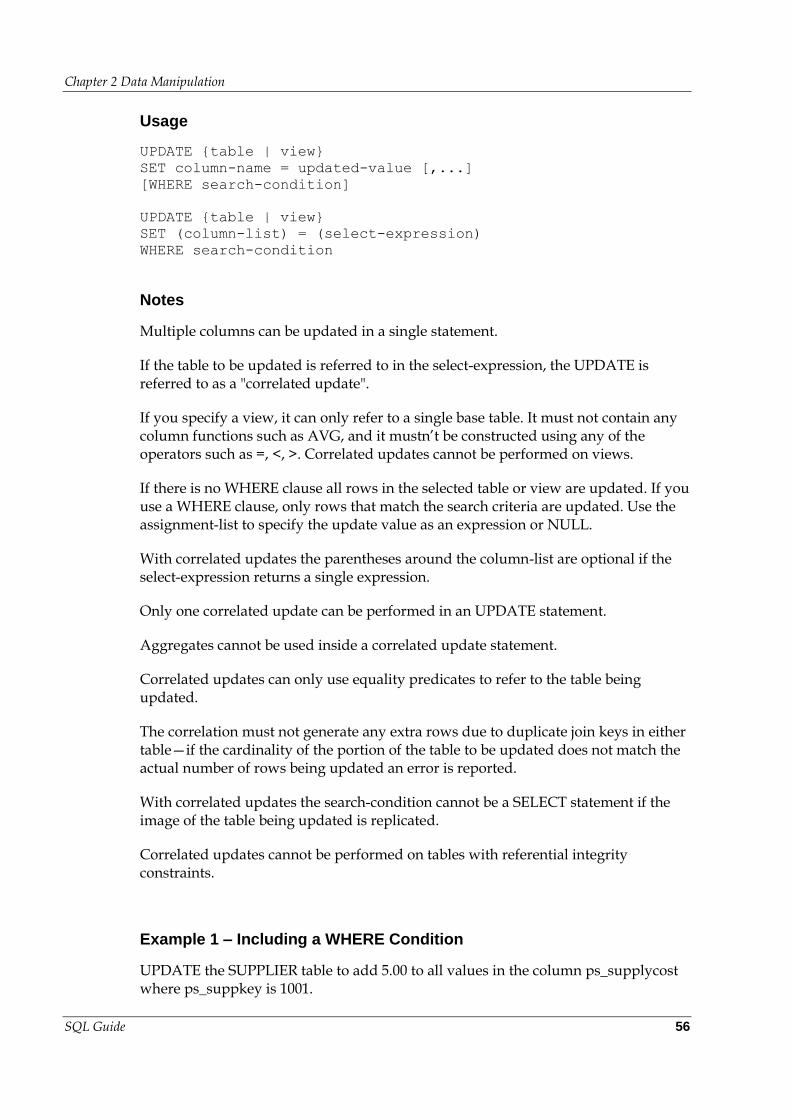
Chapter 2 Data Manipulation
SQL Guide 56
Usage
UPDATE {table | view}
SET column-name = updated-value [,...]
[WHERE search-condition]
UPDATE {table | view}
SET (column-list) = (select-expression)
WHERE search-condition
Notes
Multiple columns can be updated in a single statement.
If the table to be updated is referred to in the select-expression, the UPDATE is referred to as a "correlated update".
If you specify a view, it can only refer to a single base table. It must not contain any column functions such as AVG, and it mustn’t be constructed using any of the operators such as =, <, >. Correlated updates cannot be performed on views.
If there is no WHERE clause all rows in the selected table or view are updated. If you use a WHERE clause, only rows that match the search criteria are updated. Use the assignment-list to specify the update value as an expression or NULL.
With correlated updates the parentheses around the column-list are optional if the select-expression returns a single expression.
Only one correlated update can be performed in an UPDATE statement.
Aggregates cannot be used inside a correlated update statement.
Correlated updates can only use equality predicates to refer to the table being updated.
The correlation must not generate any extra rows due to duplicate join keys in either table—if the cardinality of the portion of the table to be updated does not match the actual number of rows being updated an error is reported.
With correlated updates the search-condition cannot be a SELECT statement if the image of the table being updated is replicated.
Correlated updates cannot be performed on tables with referential integrity constraints.
Example 1 – Including a WHERE Condition
UPDATE the SUPPLIER table to add 5.00 to all values in the column ps_supplycost where ps_suppkey is 1001.
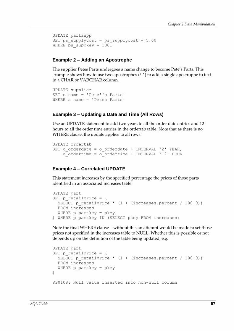
Chapter 2 Data Manipulation
SQL Guide 57
UPDATE partsupp
SET ps_supplycost = ps_supplycost + 5.00
WHERE ps_suppkey = 1001
Example 2 – Adding an Apostrophe
The supplier Petes Parts undergoes a name change to become Pete’s Parts. This example shows how to use two apostrophes (’’) to add a single apostrophe to text in a CHAR or VARCHAR column.
UPDATE supplier
SET s_name = 'Pete''s Parts'
WHERE s_name = 'Petes Parts'
Example 3 – Updating a Date and Time (All Rows)
Use an UPDATE statement to add two years to all the order date entries and 12 hours to all the order time entries in the ordertab table. Note that as there is no WHERE clause, the update applies to all rows.
UPDATE ordertab
SET o_orderdate = o_orderdate + INTERVAL '2' YEAR,
o_ordertime = o_ordertime + INTERVAL '12' HOUR
Example 4 – Correlated UPDATE
This statement increases by the specified percentage the prices of those parts identified in an associated increases table.
UPDATE part
SET p_retailprice = (
SELECT p_retailprice * (1 + (increases.percent / 100.0))
FROM increases
WHERE p_partkey = pkey
) WHERE p_partkey IN (SELECT pkey FROM increases)
Note the final WHERE clause—without this an attempt would be made to set those prices not specified in the increases table to NULL. Whether this is possible or not depends up on the definition of the table being updated, e.g.
UPDATE part
SET p_retailprice = (
SELECT p_retailprice * (1 + (increases.percent / 100.0))
FROM increases
WHERE p_partkey = pkey
)
RS0108: Null value inserted into non-null column
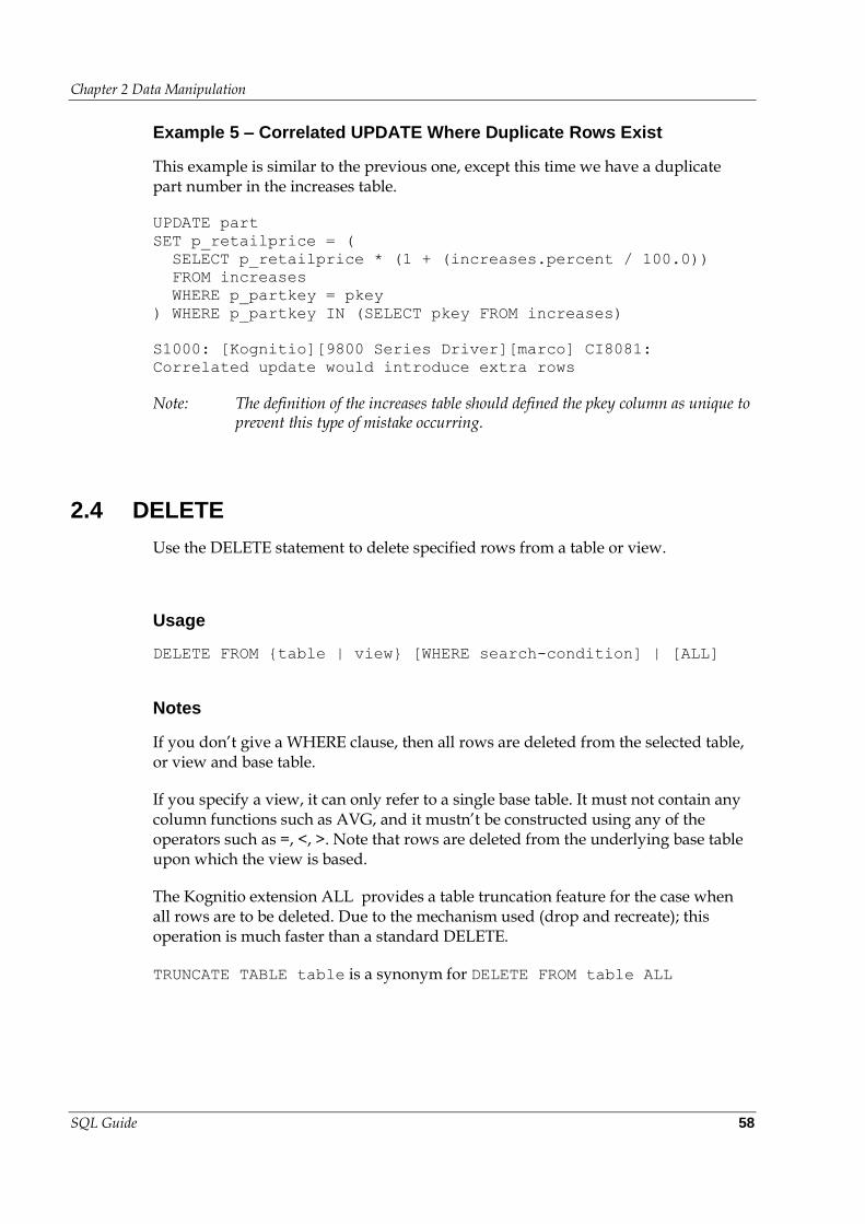
Chapter 2 Data Manipulation
SQL Guide 58
Example 5 – Correlated UPDATE Where Duplicate Rows Exist
This example is similar to the previous one, except this time we have a duplicate part number in the increases table.
UPDATE part
SET p_retailprice = (
SELECT p_retailprice * (1 + (increases.percent / 100.0))
FROM increases
WHERE p_partkey = pkey
) WHERE p_partkey IN (SELECT pkey FROM increases)
S1000: [Kognitio][9800 Series Driver][marco] CI8081:
Correlated update would introduce extra rows
Note: The definition of the increases table should defined the pkey column as unique to prevent this type of mistake occurring.
2.4 DELETE
Use the DELETE statement to delete specified rows from a table or view.
Usage
DELETE FROM {table | view} [WHERE search-condition] | [ALL]
Notes
If you don’t give a WHERE clause, then all rows are deleted from the selected table, or view and base table.
If you specify a view, it can only refer to a single base table. It must not contain any column functions such as AVG, and it mustn’t be constructed using any of the operators such as =, <, >. Note that rows are deleted from the underlying base table upon which the view is based.
The Kognitio extension ALL provides a table truncation feature for the case when all rows are to be deleted. Due to the mechanism used (drop and recreate); this operation is much faster than a standard DELETE.
TRUNCATE TABLE table is a synonym for DELETE FROM table ALL
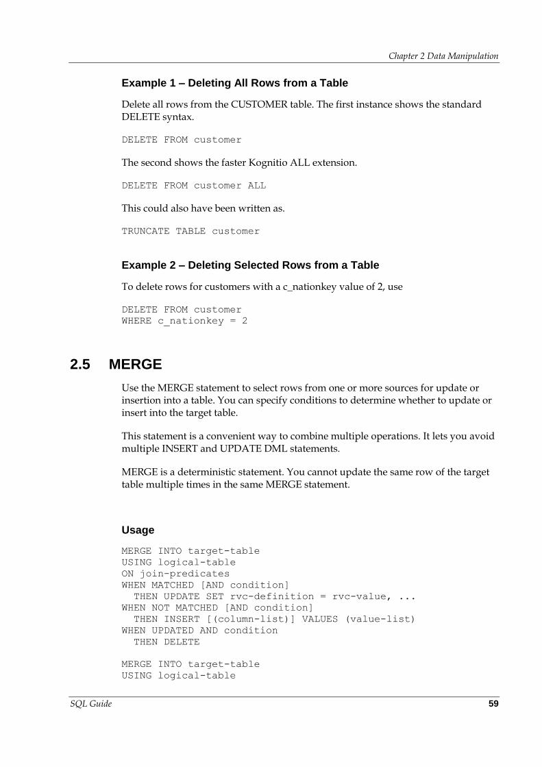
Chapter 2 Data Manipulation
SQL Guide 59
Example 1 – Deleting All Rows from a Table
Delete all rows from the CUSTOMER table. The first instance shows the standard DELETE syntax.
DELETE FROM customer
The second shows the faster Kognitio ALL extension.
DELETE FROM customer ALL
This could also have been written as.
TRUNCATE TABLE customer
Example 2 – Deleting Selected Rows from a Table
To delete rows for customers with a c_nationkey value of 2, use
DELETE FROM customer
WHERE c_nationkey = 2
2.5 MERGE
Use the MERGE statement to select rows from one or more sources for update or insertion into a table. You can specify conditions to determine whether to update or insert into the target table.
This statement is a convenient way to combine multiple operations. It lets you avoid multiple INSERT and UPDATE DML statements.
MERGE is a deterministic statement. You cannot update the same row of the target table multiple times in the same MERGE statement.
Usage
MERGE INTO target-table
USING logical-table
ON join-predicates
WHEN MATCHED [AND condition]
THEN UPDATE SET rvc-definition = rvc-value, ...
WHEN NOT MATCHED [AND condition]
THEN INSERT [(column-list)] VALUES (value-list)
WHEN UPDATED AND condition
THEN DELETE
MERGE INTO target-table
USING logical-table
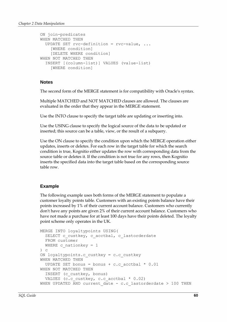
Chapter 2 Data Manipulation
SQL Guide 60
ON join-predicates
WHEN MATCHED THEN
UPDATE SET rvc-definition = rvc-value, ...
[WHERE condition]
[DELETE WHERE condition]
WHEN NOT MATCHED THEN
INSERT [(column-list)] VALUES (value-list)
[WHERE condition]
Notes
The second form of the MERGE statement is for compatibility with Oracle's syntax.
Multiple MATCHED and NOT MATCHED clauses are allowed. The clauses are evaluated in the order that they appear in the MERGE statement.
Use the INTO clause to specify the target table are updating or inserting into.
Use the USING clause to specify the logical source of the data to be updated or inserted; this source can be a table, view, or the result of a subquery.
Use the ON clause to specify the condition upon which the MERGE operation either updates, inserts or deletes. For each row in the target table for which the search condition is true, Kognitio either updates the row with corresponding data from the source table or deletes it. If the condition is not true for any rows, then Kognitio inserts the specified data into the target table based on the corresponding source table row.
Example
The following example uses both forms of the MERGE statement to populate a customer loyalty points table. Customers with an existing points balance have their points increased by 1% of their current account balance. Customers who currently don't have any points are given 2% of their current account balance. Customers who have not made a purchase for at least 100 days have their points deleted. The loyalty point scheme only operates in the UK.
MERGE INTO loyaltypoints USING(
SELECT c_custkey, c_acctbal, c_lastorderdate
FROM customer
WHERE c_nationkey = 1
) c
ON loyaltypoints.c_custkey = c.c_custkey
WHEN MATCHED THEN
UPDATE SET bonus = bonus + c.c_acctbal * 0.01
WHEN NOT MATCHED THEN
INSERT (c_custkey, bonus)
VALUES (c.c_custkey, c.c_acctbal * 0.02)
WHEN UPDATED AND current_date - c.c_lastorderdate > 100 THEN
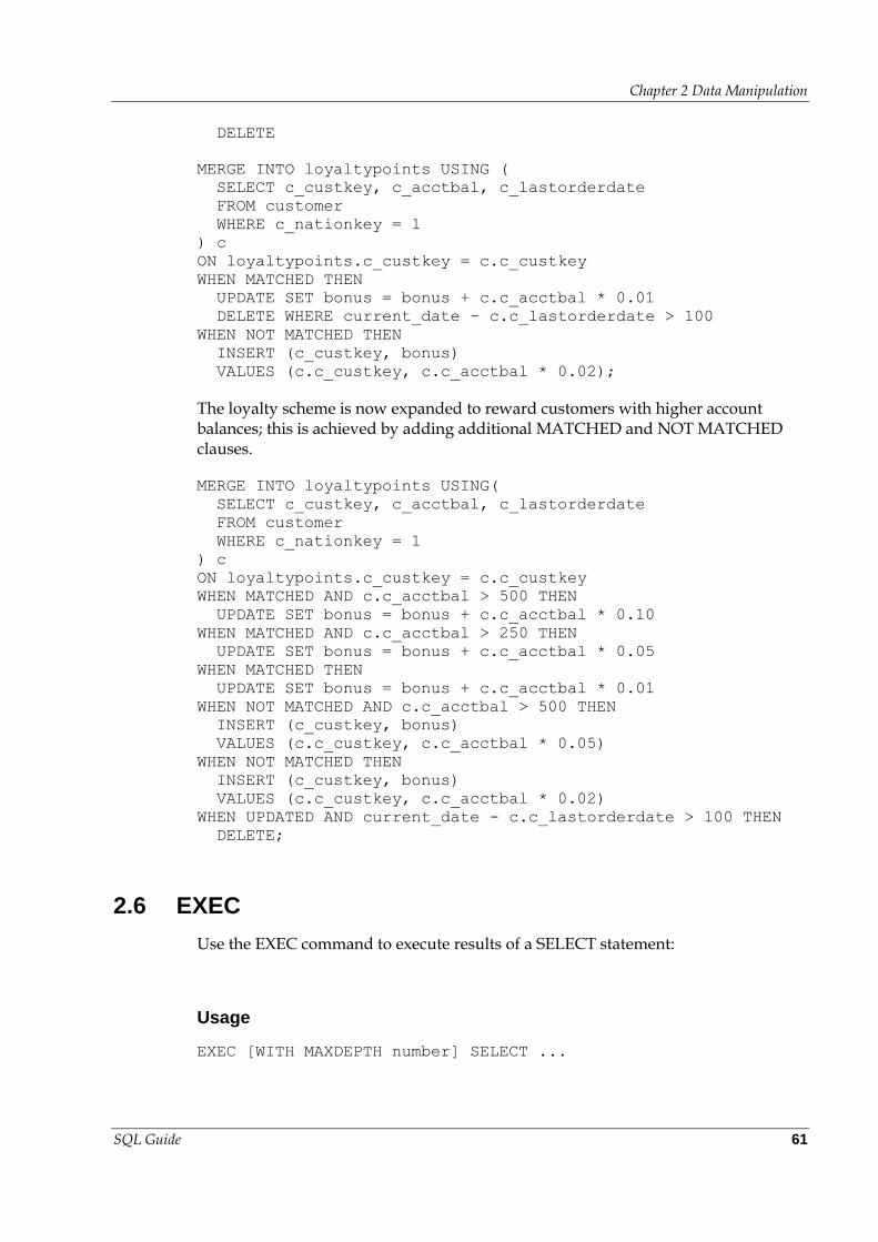
Chapter 2 Data Manipulation
SQL Guide 61
DELETE
MERGE INTO loyaltypoints USING (
SELECT c_custkey, c_acctbal, c_lastorderdate
FROM customer
WHERE c_nationkey = 1
) c
ON loyaltypoints.c_custkey = c.c_custkey
WHEN MATCHED THEN
UPDATE SET bonus = bonus + c.c_acctbal * 0.01
DELETE WHERE current_date - c.c_lastorderdate > 100
WHEN NOT MATCHED THEN
INSERT (c_custkey, bonus)
VALUES (c.c_custkey, c.c_acctbal * 0.02);
The loyalty scheme is now expanded to reward customers with higher account balances; this is achieved by adding additional MATCHED and NOT MATCHED clauses.
MERGE INTO loyaltypoints USING(
SELECT c_custkey, c_acctbal, c_lastorderdate
FROM customer
WHERE c_nationkey = 1
) c
ON loyaltypoints.c_custkey = c.c_custkey
WHEN MATCHED AND c.c_acctbal > 500 THEN
UPDATE SET bonus = bonus + c.c_acctbal * 0.10
WHEN MATCHED AND c.c_acctbal > 250 THEN
UPDATE SET bonus = bonus + c.c_acctbal * 0.05
WHEN MATCHED THEN
UPDATE SET bonus = bonus + c.c_acctbal * 0.01
WHEN NOT MATCHED AND c.c_acctbal > 500 THEN
INSERT (c_custkey, bonus)
VALUES (c.c_custkey, c.c_acctbal * 0.05)
WHEN NOT MATCHED THEN
INSERT (c_custkey, bonus)
VALUES (c.c_custkey, c.c_acctbal * 0.02)
WHEN UPDATED AND current_date - c.c_lastorderdate > 100 THEN
DELETE;
2.6 EXEC
Use the EXEC command to execute results of a SELECT statement:
Usage
EXEC [WITH MAXDEPTH number] SELECT ...
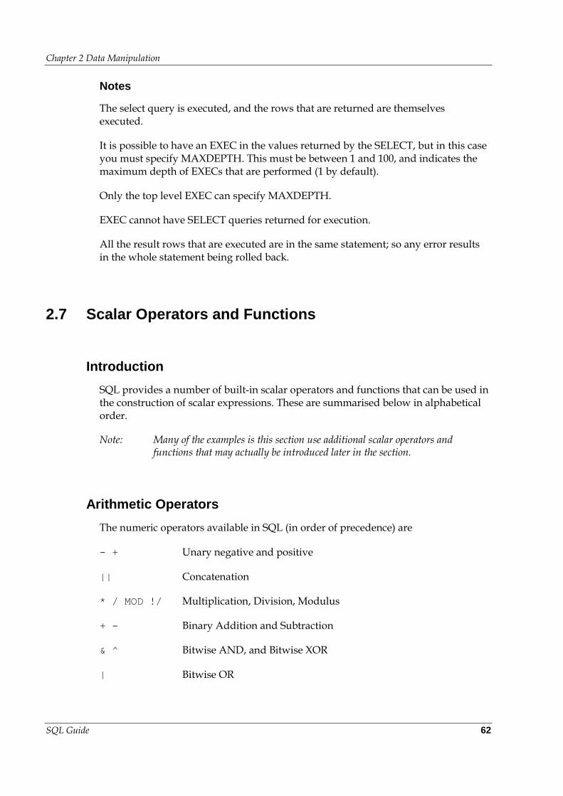
Chapter 2 Data Manipulation
SQL Guide 62
Notes
The select query is executed, and the rows that are returned are themselves executed.
It is possible to have an EXEC in the values returned by the SELECT, but in this case you must specify MAXDEPTH. This must be between 1 and 100, and indicates the maximum depth of EXECs that are performed (1 by default).
Only the top level EXEC can specify MAXDEPTH.
EXEC cannot have SELECT queries returned for execution.
All the result rows that are executed are in the same statement; so any error results in the whole statement being rolled back.
2.7 Scalar Operators and Functions
Introduction
SQL provides a number of built-in scalar operators and functions that can be used in the construction of scalar expressions. These are summarised below in alphabetical order.
Note: Many of the examples is this section use additional scalar operators and functions that may actually be introduced later in the section.
Arithmetic Operators
The numeric operators available in SQL (in order of precedence) are
- + Unary negative and positive
|| Concatenation
* / MOD !/ Multiplication, Division, Modulus
+ - Binary Addition and Subtraction
& ^ Bitwise AND, and Bitwise XOR
| Bitwise OR
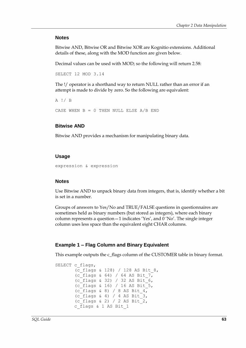
Chapter 2 Data Manipulation
SQL Guide 63
Notes
Bitwise AND, Bitwise OR and Bitwise XOR are Kognitio extensions. Additional details of these, along with the MOD function are given below.
Decimal values can be used with MOD; so the following will return 2.58:
SELECT 12 MOD 3.14
The !/ operator is a shorthand way to return NULL rather than an error if an attempt is made to divide by zero. So the following are equivalent:
A !/ B
CASE WHEN B = 0 THEN NULL ELSE A/B END
Bitwise AND
Bitwise AND provides a mechanism for manipulating binary data.
Usage
expression & expression
Notes
Use Bitwise AND to unpack binary data from integers, that is, identify whether a bit is set in a number.
Groups of answers to Yes/No and TRUE/FALSE questions in questionnaires are sometimes held as binary numbers (but stored as integers), where each binary column represents a question—1 indicates ‘Yes’, and 0 ‘No’. The single integer column uses less space than the equivalent eight CHAR columns.
Example 1 – Flag Column and Binary Equivalent
This example outputs the c_flags column of the CUSTOMER table in binary format.
SELECT c_flags,
(c_flags & 128) / 128 AS Bit_8,
(c_flags & 64) / 64 AS Bit_7,
(c_flags & 32) / 32 AS Bit_6,
(c_flags & 16) / 16 AS Bit_5,
(c_flags & 8) / 8 AS Bit_4,
(c_flags & 4) / 4 AS Bit_3,
(c_flags & 2) / 2 AS Bit_2,
c_flags & 1 AS Bit_1
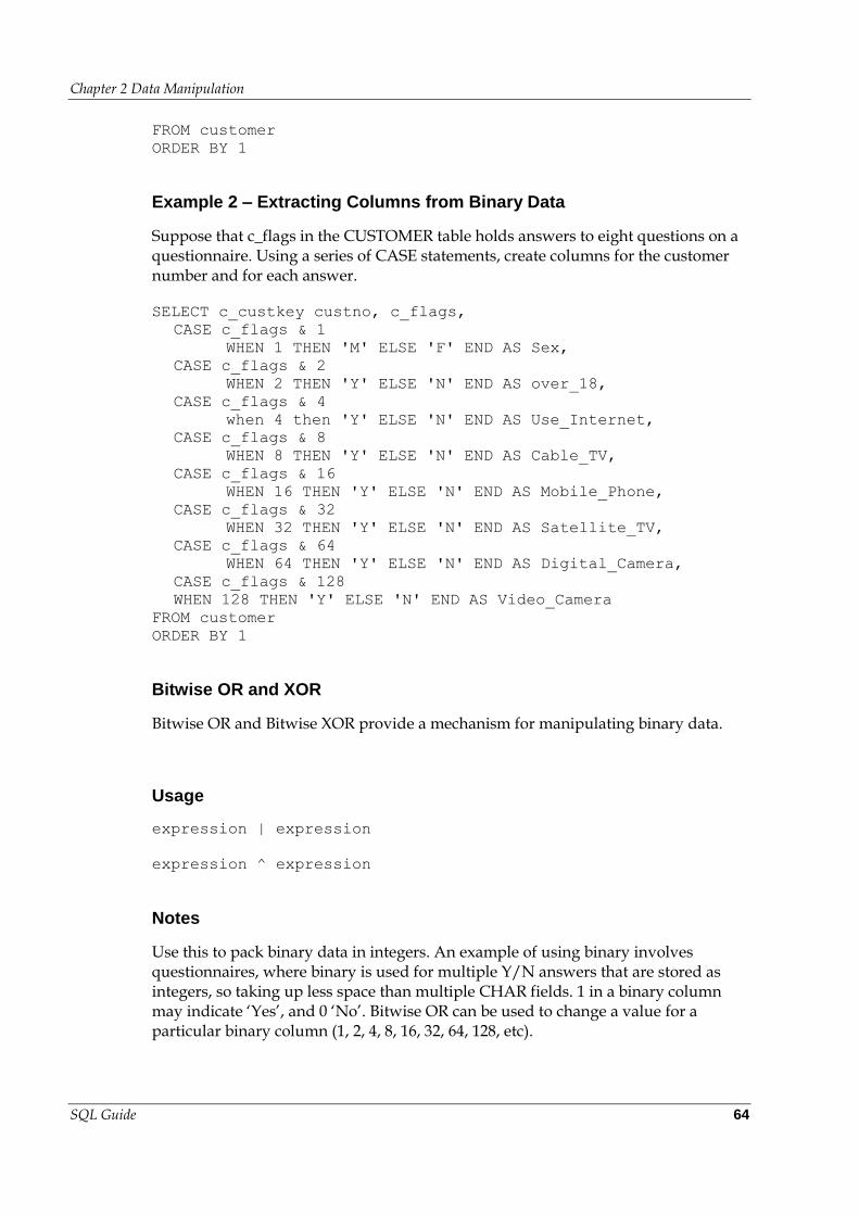
Chapter 2 Data Manipulation
SQL Guide 64
FROM customer
ORDER BY 1
Example 2 – Extracting Columns from Binary Data
Suppose that c_flags in the CUSTOMER table holds answers to eight questions on a questionnaire. Using a series of CASE statements, create columns for the customer number and for each answer.
SELECT c_custkey custno, c_flags,
CASE c_flags & 1
WHEN 1 THEN 'M' ELSE 'F' END AS Sex,
CASE c_flags & 2
WHEN 2 THEN 'Y' ELSE 'N' END AS over_18,
CASE c_flags & 4
when 4 then 'Y' ELSE 'N' END AS Use_Internet,
CASE c_flags & 8
WHEN 8 THEN 'Y' ELSE 'N' END AS Cable_TV,
CASE c_flags & 16
WHEN 16 THEN 'Y' ELSE 'N' END AS Mobile_Phone,
CASE c_flags & 32
WHEN 32 THEN 'Y' ELSE 'N' END AS Satellite_TV,
CASE c_flags & 64
WHEN 64 THEN 'Y' ELSE 'N' END AS Digital_Camera,
CASE c_flags & 128
WHEN 128 THEN 'Y' ELSE 'N' END AS Video_Camera
FROM customer
ORDER BY 1
Bitwise OR and XOR
Bitwise OR and Bitwise XOR provide a mechanism for manipulating binary data.
Usage
expression | expression
expression ^ expression
Notes
Use this to pack binary data in integers. An example of using binary involves questionnaires, where binary is used for multiple Y/N answers that are stored as integers, so taking up less space than multiple CHAR fields. 1 in a binary column may indicate ‘Yes’, and 0 ‘No’. Bitwise OR can be used to change a value for a particular binary column (1, 2, 4, 8, 16, 32, 64, 128, etc).
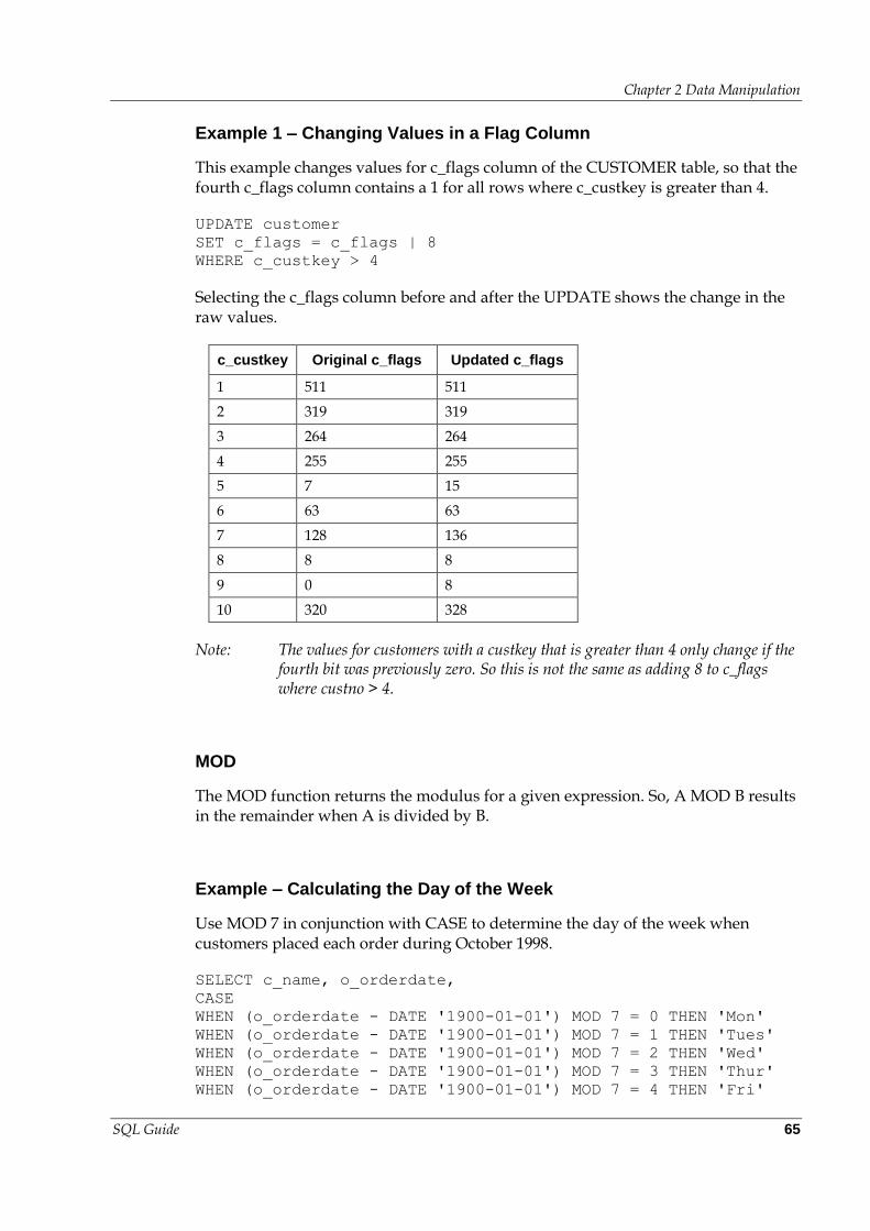
Chapter 2 Data Manipulation
SQL Guide 65
Example 1 – Changing Values in a Flag Column
This example changes values for c_flags column of the CUSTOMER table, so that the fourth c_flags column contains a 1 for all rows where c_custkey is greater than 4.
UPDATE customer
SET c_flags = c_flags | 8
WHERE c_custkey > 4
Selecting the c_flags column before and after the UPDATE shows the change in the raw values.
c_custkey Original c_flags Updated c_flags
1 511 511
2 319 319
3 264 264
4 255 255
5 7 15
6 63 63
7 128 136
8 8 8
9 0 8
10 320 328
Note: The values for customers with a custkey that is greater than 4 only change if the fourth bit was previously zero. So this is not the same as adding 8 to c_flags where custno > 4.
MOD
The MOD function returns the modulus for a given expression. So, A MOD B results in the remainder when A is divided by B.
Example – Calculating the Day of the Week
Use MOD 7 in conjunction with CASE to determine the day of the week when customers placed each order during October 1998.
SELECT c_name, o_orderdate,
CASE
WHEN (o_orderdate - DATE '1900-01-01') MOD 7 = 0 THEN 'Mon'
WHEN (o_orderdate - DATE '1900-01-01') MOD 7 = 1 THEN 'Tues'
WHEN (o_orderdate - DATE '1900-01-01') MOD 7 = 2 THEN 'Wed'
WHEN (o_orderdate - DATE '1900-01-01') MOD 7 = 3 THEN 'Thur'
WHEN (o_orderdate - DATE '1900-01-01') MOD 7 = 4 THEN 'Fri'
Chapter 2 Data Manipulation
SQL Guide 66
WHEN (o_orderdate - DATE '1900-01-01') MOD 7 = 5 THEN 'Sat'
WHEN (o_orderdate - DATE '1900-01-01') MOD 7 = 6 THEN 'Sun'
END weekday
FROM customer, ordertab
WHERE c_custkey = o_custkey AND
o_orderdate BETWEEN DATE '1998-10-01' AND
DATE '1998-10-31'
ORDER BY 1
Note: This is based on the fact that 1st January 1900 was a Monday. An easier way to calculate the day of the week is to use the DAYOFWEEK() function.
ABS
The ABS function returns the absolute value of the supplied argument.
Usage
ABS(argument)
Notes
The single argument for the ABS function must be either NUMERIC or an INTERVAL. The result is the absolute (positive) value of the argument and is of the same data type as the argument. An error occurs if the argument has an invalid data type, or if the maximum negative value for the INTEGER data types is passed to the function.
Example
Obtain "recent orders", that is, orders delivered in the last month, or expected in the next month.
SELECT o_orderkey, o_deliverytime,
ABS(CURRENT_DATE - CAST(o_deliverytime AS DATE)) Days
FROM ordertab2
WHERE ABS(CURRENT_DATE - CAST(o_deliverytime AS DATE)) < 30
ORDER BY 3 DESC, 2, 1
ACOS
ACOS calculates the inverse cosine for the specified argument.
Chapter 2 Data Manipulation
SQL Guide 67
Usage
ACOS(argument)
Notes
The argument must be NUMERIC. An error occurs if the argument has an invalid data type, or if the result is too large to be represented by a FLOAT.
ASCII
ASCII returns the integer representation of a character.
Usage
ASCII(char)
Notes
char is a single CHARACTER value.
See CHR for an example of using the ASCII function.
ASIN
ASIN calculates the inverse sine for the specified argument.
Usage
ASIN(argument)
Notes
The argument must be NUMERIC. An error occurs if the argument has an invalid data type, or if the result is too large to be represented by a FLOAT.
ATAN
ATAN calculates the inverse tangent for the specified argument.
Chapter 2 Data Manipulation
SQL Guide 68
Usage
ATAN(argument)
Notes
The argument must be NUMERIC. An error occurs if the argument has an invalid data type, or if the result is too large to be represented by a FLOAT.
CASE
Simple Case Expression
The result of a simple CASE expression is the result expression associated with the first value expression that equals the test expression. If no value expression equals the test expression, the result is the default result, or NULL if no default is specified.
Usage
CASE test-expression
WHEN value-expression THEN result-expression | NULL
[WHEN value-expression THEN result-expression | NULL]...
[ELSE default-result-expression | NULL]
END
Searched Case Expression
The result of a searched CASE expression is the first result expression for which the associated search condition evaluates to ‘TRUE’. If no search condition evaluates to TRUE, the result is either the default result, or NULL if no default is specified.
Usage
CASE
WHEN search-condition THEN result-expression | NULL
[WHEN search-condition THEN result-expression | NULL]...
[ELSE default-result-expression | NULL]
END
Note: It is possible to write the CASE expression with a comma separated list of search-conditions that have the same result-expression.
Chapter 2 Data Manipulation
SQL Guide 69
Example 1 – The Two Forms of CASE
Extract nationality data using both forms of the CASE statement from the SUPPLIER table.
SELECT s_name supplier,
CASE s_nationkey
WHEN 1 THEN 'British'
WHEN 2 THEN 'American'
WHEN 3 THEN 'European'
WHEN 4 THEN 'European'
WHEN 5 THEN 'European'
ELSE 'nationality unknown'
END nationality
FROM supplier
SELECT s_name supplier,
CASE s_nationkey
WHEN 1 THEN 'British'
WHEN 2 THEN 'American'
WHEN 3, 4, 5 THEN 'European'
ELSE 'nationality unknown'
END nationality
FROM supplier
SELECT s_name supplier,
CASE
WHEN s_nationkey = 1 THEN 'British'
WHEN s_nationkey = 2 THEN 'American'
WHEN s_nationkey = 3,
s_nationkey = 4,
s_nationkey = 5 THEN 'European'
ELSE 'nationality unknown'
END nationality
FROM supplier
Note: The above examples have been written to show the various forms of the comma separated list of search-conditions.
Example 2 – Order Priorities
This query that uses CASE to display the order numbers, date of order, and when the order should be delivered based on the order priority.
SELECT o_orderkey, o_orderdate, o_orderpriority,
CASE LOWER(o_orderpriority)
WHEN 'high' THEN o_orderdate + INTERVAL '1' DAY
WHEN 'med' THEN o_orderdate + INTERVAL '7' DAY
WHEN 'low' THEN o_orderdate + INTERVAL '1' MONTH
END AS ShipBy
FROM ordertab
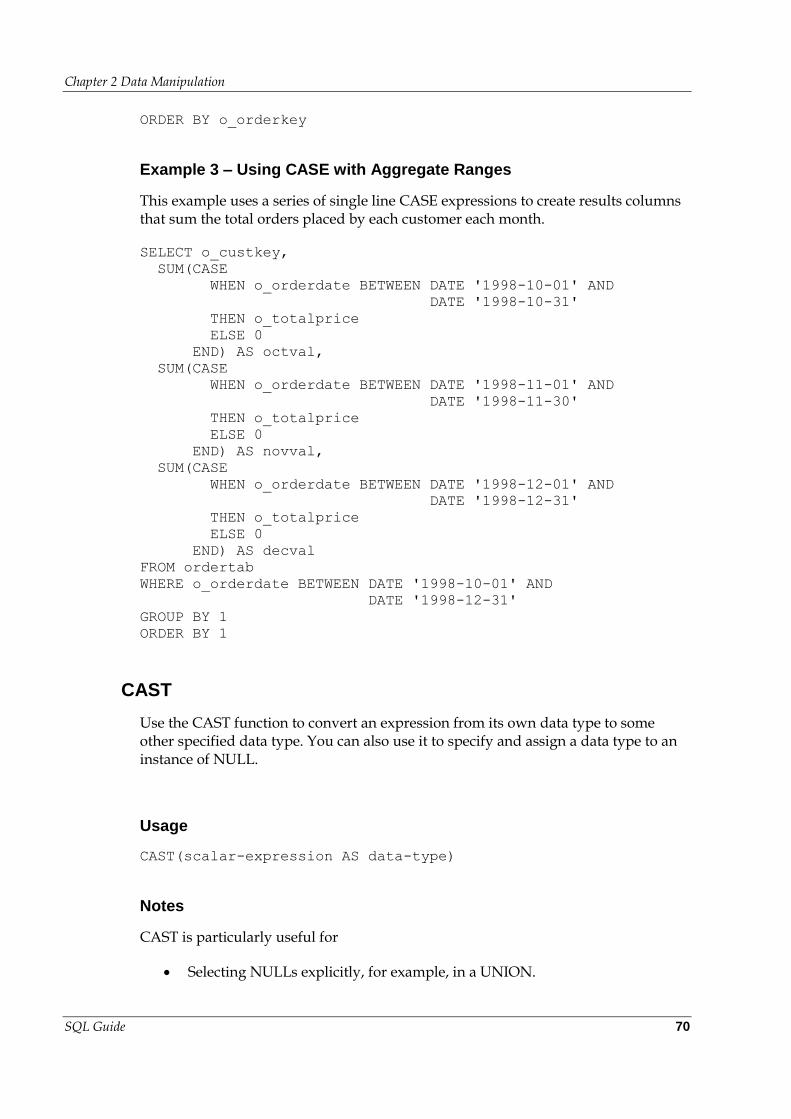
Chapter 2 Data Manipulation
SQL Guide 70
ORDER BY o_orderkey
Example 3 – Using CASE with Aggregate Ranges
This example uses a series of single line CASE expressions to create results columns that sum the total orders placed by each customer each month.
SELECT o_custkey,
SUM(CASE
WHEN o_orderdate BETWEEN DATE '1998-10-01' AND
DATE '1998-10-31'
THEN o_totalprice
ELSE 0
END) AS octval,
SUM(CASE
WHEN o_orderdate BETWEEN DATE '1998-11-01' AND
DATE '1998-11-30'
THEN o_totalprice
ELSE 0
END) AS novval,
SUM(CASE
WHEN o_orderdate BETWEEN DATE '1998-12-01' AND
DATE '1998-12-31'
THEN o_totalprice
ELSE 0
END) AS decval
FROM ordertab
WHERE o_orderdate BETWEEN DATE '1998-10-01' AND
DATE '1998-12-31'
GROUP BY 1
ORDER BY 1
CAST
Use the CAST function to convert an expression from its own data type to some other specified data type. You can also use it to specify and assign a data type to an instance of NULL.
Usage
CAST(scalar-expression AS data-type)
Notes
CAST is particularly useful for
Selecting NULLs explicitly, for example, in a UNION.
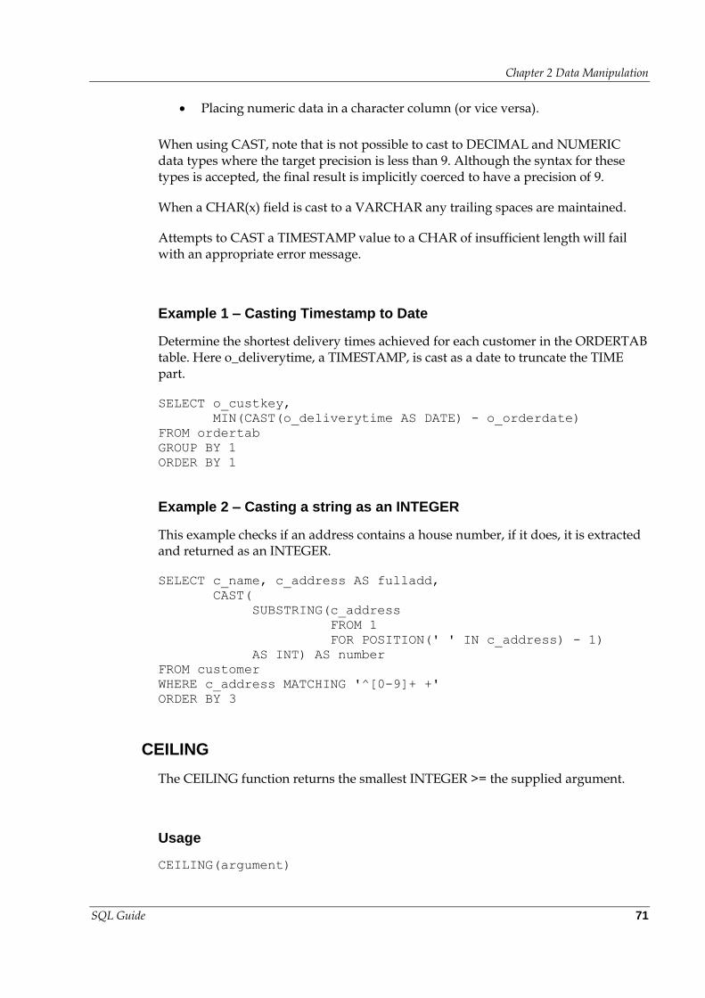
Chapter 2 Data Manipulation
SQL Guide 71
Placing numeric data in a character column (or vice versa).
When using CAST, note that is not possible to cast to DECIMAL and NUMERIC data types where the target precision is less than 9. Although the syntax for these types is accepted, the final result is implicitly coerced to have a precision of 9.
When a CHAR(x) field is cast to a VARCHAR any trailing spaces are maintained.
Attempts to CAST a TIMESTAMP value to a CHAR of insufficient length will fail with an appropriate error message.
Example 1 – Casting Timestamp to Date
Determine the shortest delivery times achieved for each customer in the ORDERTAB table. Here o_deliverytime, a TIMESTAMP, is cast as a date to truncate the TIME part.
SELECT o_custkey,
MIN(CAST(o_deliverytime AS DATE) - o_orderdate)
FROM ordertab
GROUP BY 1
ORDER BY 1
Example 2 – Casting a string as an INTEGER
This example checks if an address contains a house number, if it does, it is extracted and returned as an INTEGER.
SELECT c_name, c_address AS fulladd,
CAST(
SUBSTRING(c_address
FROM 1
FOR POSITION(' ' IN c_address) - 1)
AS INT) AS number
FROM customer
WHERE c_address MATCHING '^[0-9]+ +'
ORDER BY 3
CEILING
The CEILING function returns the smallest INTEGER >= the supplied argument.
Usage
CEILING(argument)
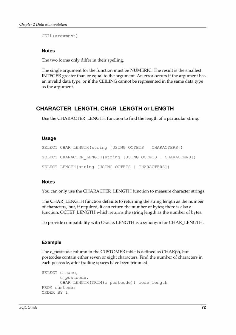
Chapter 2 Data Manipulation
SQL Guide 72
CEIL(argument)
Notes
The two forms only differ in their spelling.
The single argument for the function must be NUMERIC. The result is the smallest INTEGER greater than or equal to the argument. An error occurs if the argument has an invalid data type, or if the CEILING cannot be represented in the same data type as the argument.
CHARACTER_LENGTH, CHAR_LENGTH or LENGTH
Use the CHARACTER_LENGTH function to find the length of a particular string.
Usage
SELECT CHAR_LENGTH(string [USING OCTETS | CHARACTERS])
SELECT CHARACTER_LENGTH(string [USING OCTETS | CHARACTERS])
SELECT LENGTH(string [USING OCTETS | CHARACTERS])
Notes
You can only use the CHARACTER_LENGTH function to measure character strings.
The CHAR_LENGTH function defaults to returning the string length as the number of characters, but, if required, it can return the number of bytes; there is also a function, OCTET_LENGTH which returns the string length as the number of bytes:
To provide compatibility with Oracle, LENGTH is a synonym for CHAR_LENGTH.
Example
The c_postcode column in the CUSTOMER table is defined as CHAR(9), but postcodes contain either seven or eight characters. Find the number of characters in each postcode, after trailing spaces have been trimmed.
SELECT c_name,
c_postcode,
CHAR_LENGTH(TRIM(c_postcode)) code_length
FROM customer
ORDER BY 1
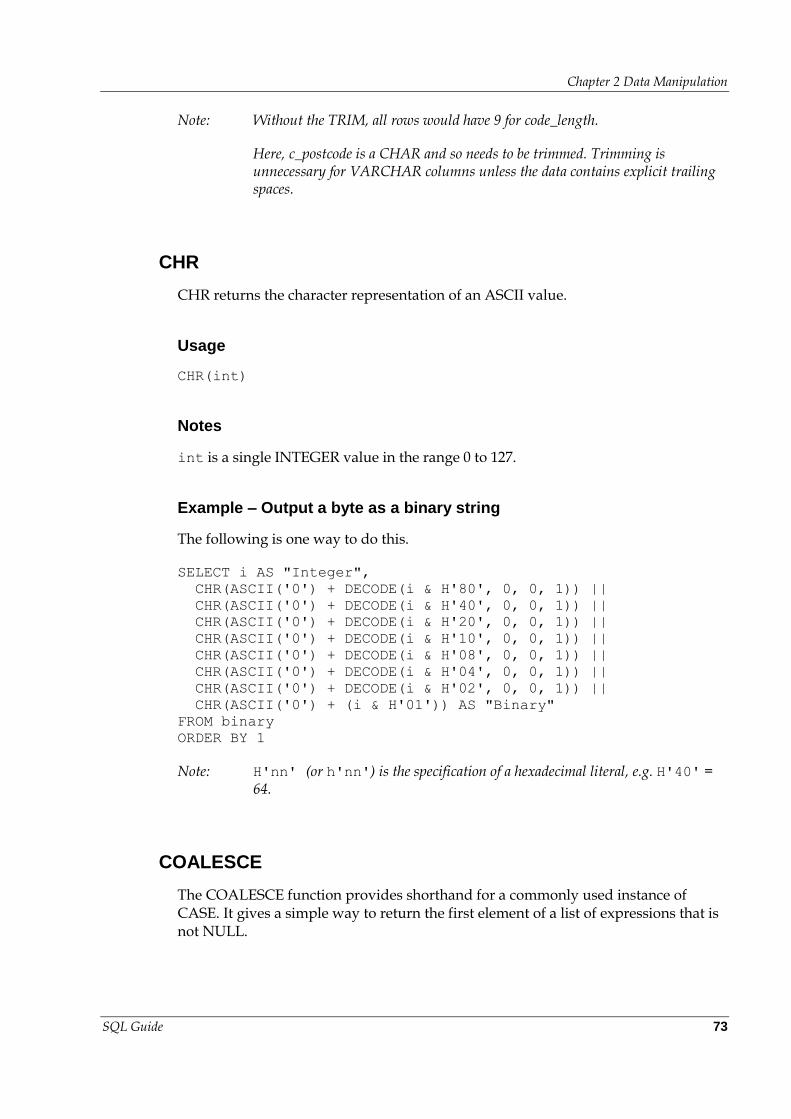
Chapter 2 Data Manipulation
SQL Guide 73
Note: Without the TRIM, all rows would have 9 for code_length.
Here, c_postcode is a CHAR and so needs to be trimmed. Trimming is unnecessary for VARCHAR columns unless the data contains explicit trailing spaces.
CHR
CHR returns the character representation of an ASCII value.
Usage
CHR(int)
Notes
int is a single INTEGER value in the range 0 to 127.
Example – Output a byte as a binary string
The following is one way to do this.
SELECT i AS "Integer",
CHR(ASCII('0') + DECODE(i & H'80', 0, 0, 1)) ||
CHR(ASCII('0') + DECODE(i & H'40', 0, 0, 1)) ||
CHR(ASCII('0') + DECODE(i & H'20', 0, 0, 1)) ||
CHR(ASCII('0') + DECODE(i & H'10', 0, 0, 1)) ||
CHR(ASCII('0') + DECODE(i & H'08', 0, 0, 1)) ||
CHR(ASCII('0') + DECODE(i & H'04', 0, 0, 1)) ||
CHR(ASCII('0') + DECODE(i & H'02', 0, 0, 1)) ||
CHR(ASCII('0') + (i & H'01')) AS "Binary"
FROM binary
ORDER BY 1
Note: H'nn' (or h'nn') is the specification of a hexadecimal literal, e.g. H'40' = 64.
COALESCE
The COALESCE function provides shorthand for a commonly used instance of CASE. It gives a simple way to return the first element of a list of expressions that is not NULL.
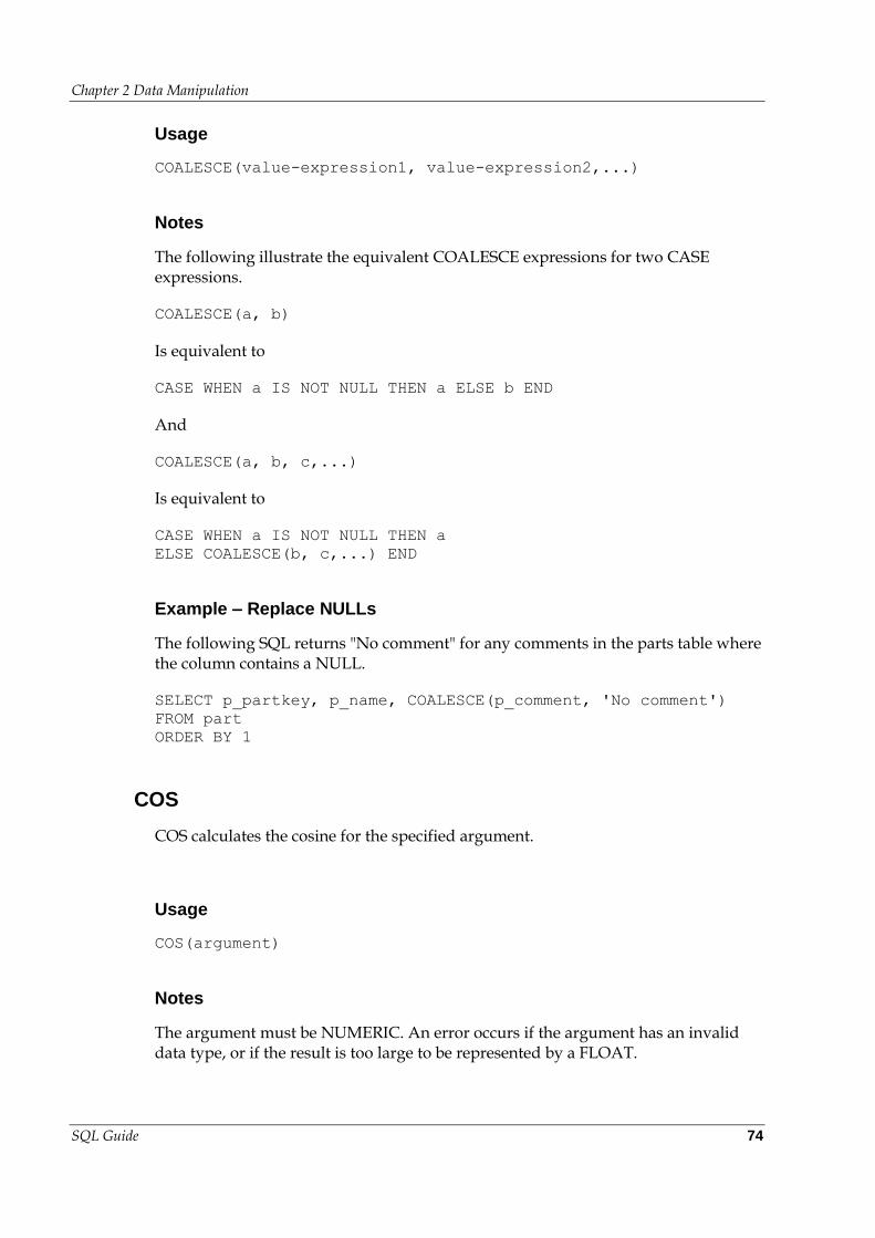
Chapter 2 Data Manipulation
SQL Guide 74
Usage
COALESCE(value-expression1, value-expression2,...)
Notes
The following illustrate the equivalent COALESCE expressions for two CASE expressions.
COALESCE(a, b)
Is equivalent to
CASE WHEN a IS NOT NULL THEN a ELSE b END
And
COALESCE(a, b, c,...)
Is equivalent to
CASE WHEN a IS NOT NULL THEN a
ELSE COALESCE(b, c,...) END
Example – Replace NULLs
The following SQL returns "No comment" for any comments in the parts table where the column contains a NULL.
SELECT p_partkey, p_name, COALESCE(p_comment, 'No comment')
FROM part
ORDER BY 1
COS
COS calculates the cosine for the specified argument.
Usage
COS(argument)
Notes
The argument must be NUMERIC. An error occurs if the argument has an invalid data type, or if the result is too large to be represented by a FLOAT.
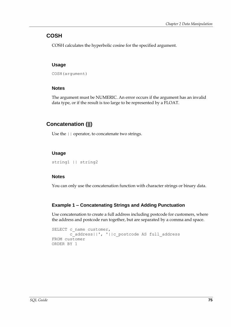
Chapter 2 Data Manipulation
SQL Guide 75
COSH
COSH calculates the hyperbolic cosine for the specified argument.
Usage
COSH(argument)
Notes
The argument must be NUMERIC. An error occurs if the argument has an invalid data type, or if the result is too large to be represented by a FLOAT.
Concatenation (||)
Use the || operator, to concatenate two strings.
Usage
string1 || string2
Notes
You can only use the concatenation function with character strings or binary data.
Example 1 – Concatenating Strings and Adding Punctuation
Use concatenation to create a full address including postcode for customers, where the address and postcode run together, but are separated by a comma and space.
SELECT c_name customer,
c_address||', '||c_postcode AS full_address
FROM customer
ORDER BY 1
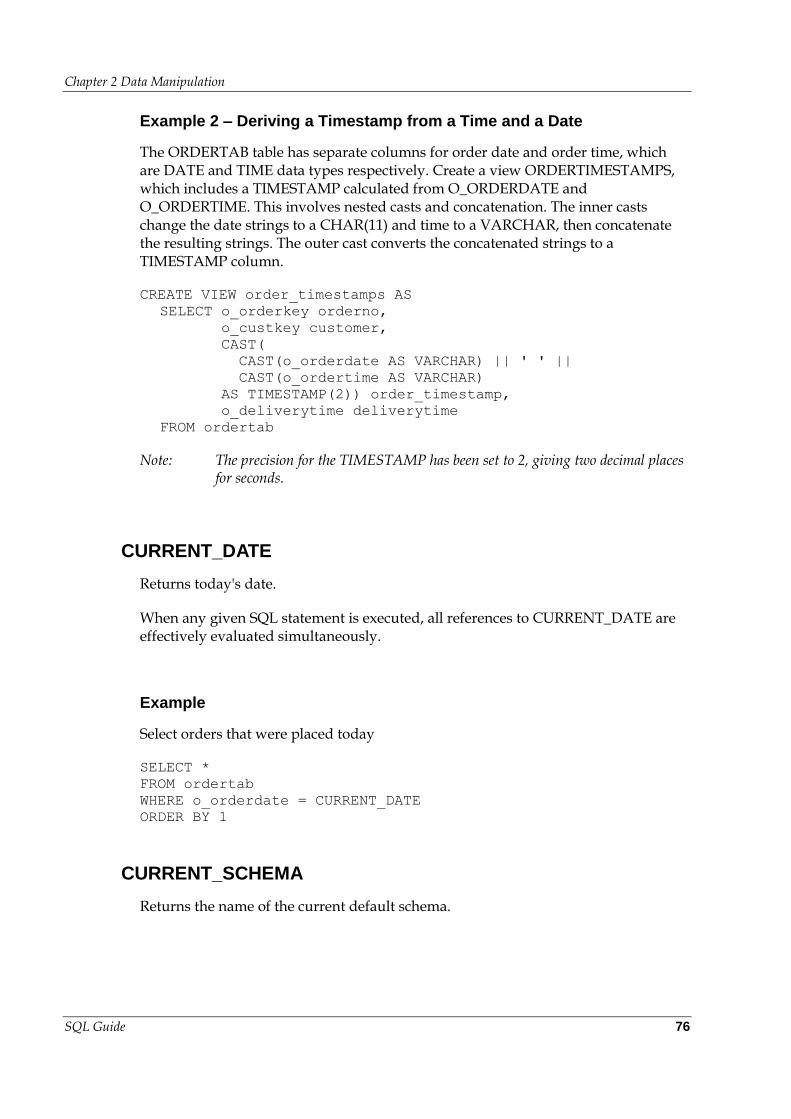
Chapter 2 Data Manipulation
SQL Guide 76
Example 2 – Deriving a Timestamp from a Time and a Date
The ORDERTAB table has separate columns for order date and order time, which are DATE and TIME data types respectively. Create a view ORDERTIMESTAMPS, which includes a TIMESTAMP calculated from O_ORDERDATE and O_ORDERTIME. This involves nested casts and concatenation. The inner casts change the date strings to a CHAR(11) and time to a VARCHAR, then concatenate the resulting strings. The outer cast converts the concatenated strings to a TIMESTAMP column.
CREATE VIEW order_timestamps AS
SELECT o_orderkey orderno,
o_custkey customer,
CAST(
CAST(o_orderdate AS VARCHAR) || ' ' ||
CAST(o_ordertime AS VARCHAR)
AS TIMESTAMP(2)) order_timestamp,
o_deliverytime deliverytime
FROM ordertab
Note: The precision for the TIMESTAMP has been set to 2, giving two decimal places for seconds.
CURRENT_DATE
Returns today's date.
When any given SQL statement is executed, all references to CURRENT_DATE are effectively evaluated simultaneously.
Example
Select orders that were placed today
SELECT *
FROM ordertab
WHERE o_orderdate = CURRENT_DATE
ORDER BY 1
CURRENT_SCHEMA
Returns the name of the current default schema.
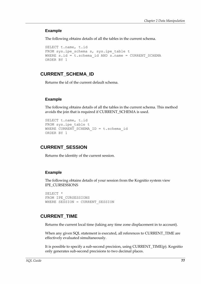
Chapter 2 Data Manipulation
SQL Guide 77
Example
The following obtains details of all the tables in the current schema.
SELECT t.name, t.id
FROM sys.ipe_schema s, sys.ipe_table t
WHERE s.id = t.schema_id AND s.name = CURRENT_SCHEMA
ORDER BY 1
CURRENT_SCHEMA_ID
Returns the id of the current default schema.
Example
The following obtains details of all the tables in the current schema. This method avoids the join that is required if CURRENT_SCHEMA is used.
SELECT t.name, t.id
FROM sys.ipe_table t
WHERE CURRENT_SCHEMA_ID = t.schema_id
ORDER BY 1
CURRENT_SESSION
Returns the identity of the current session.
Example
The following obtains details of your session from the Kognitio system view IPE_CURSESSIONS
SELECT *
FROM IPE_CURSESSIONS
WHERE SESSION = CURRENT_SESSION
CURRENT_TIME
Returns the current local time (taking any time zone displacement in to account).
When any given SQL statement is executed, all references to CURRENT_TIME are effectively evaluated simultaneously.
It is possible to specify a sub-second precision, using CURRENT_TIME(p). Kognitio only generates sub-second precisions to two decimal places.
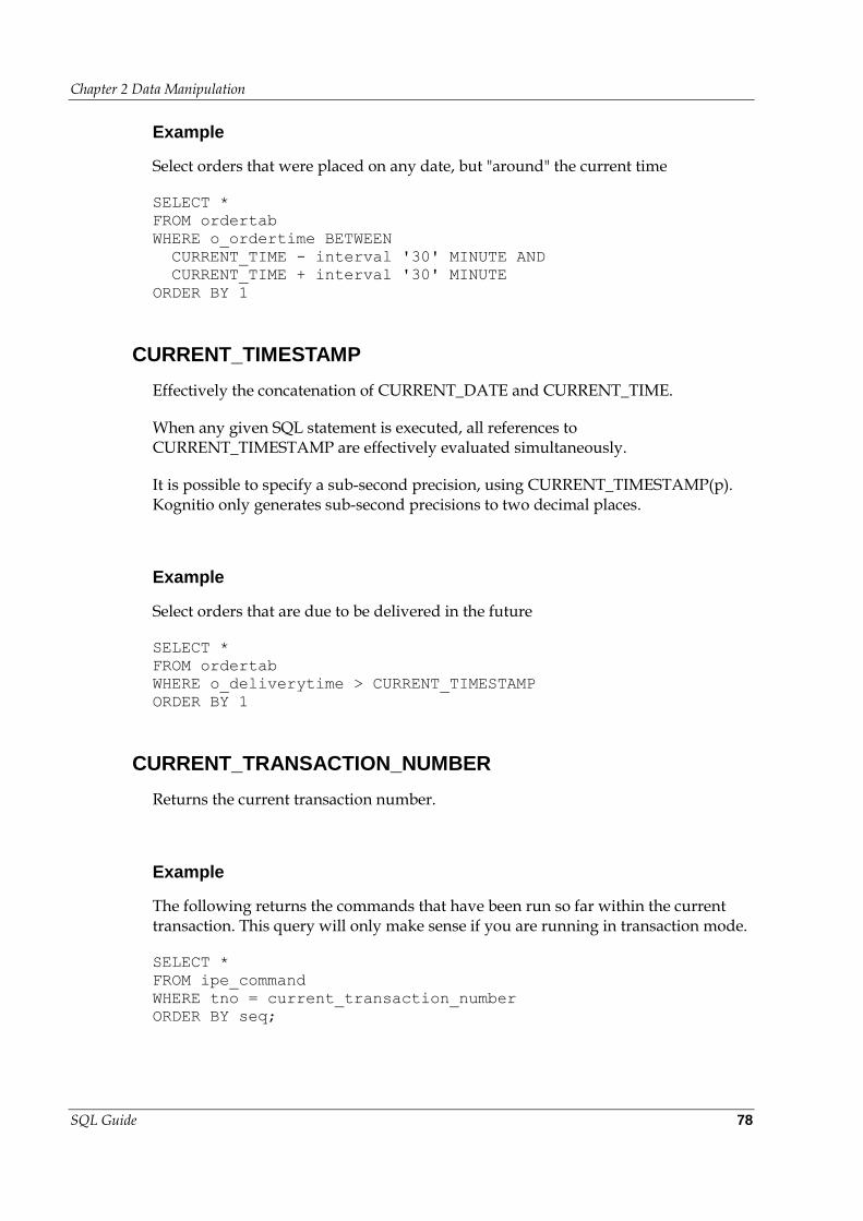
Chapter 2 Data Manipulation
SQL Guide 78
Example
Select orders that were placed on any date, but "around" the current time
SELECT *
FROM ordertab
WHERE o_ordertime BETWEEN
CURRENT_TIME - interval '30' MINUTE AND
CURRENT_TIME + interval '30' MINUTE
ORDER BY 1
CURRENT_TIMESTAMP
Effectively the concatenation of CURRENT_DATE and CURRENT_TIME.
When any given SQL statement is executed, all references to CURRENT_TIMESTAMP are effectively evaluated simultaneously.
It is possible to specify a sub-second precision, using CURRENT_TIMESTAMP(p). Kognitio only generates sub-second precisions to two decimal places.
Example
Select orders that are due to be delivered in the future
SELECT *
FROM ordertab
WHERE o_deliverytime > CURRENT_TIMESTAMP
ORDER BY 1
CURRENT_TRANSACTION_NUMBER
Returns the current transaction number.
Example
The following returns the commands that have been run so far within the current transaction. This query will only make sense if you are running in transaction mode.
SELECT *
FROM ipe_command
WHERE tno = current_transaction_number
ORDER BY seq;
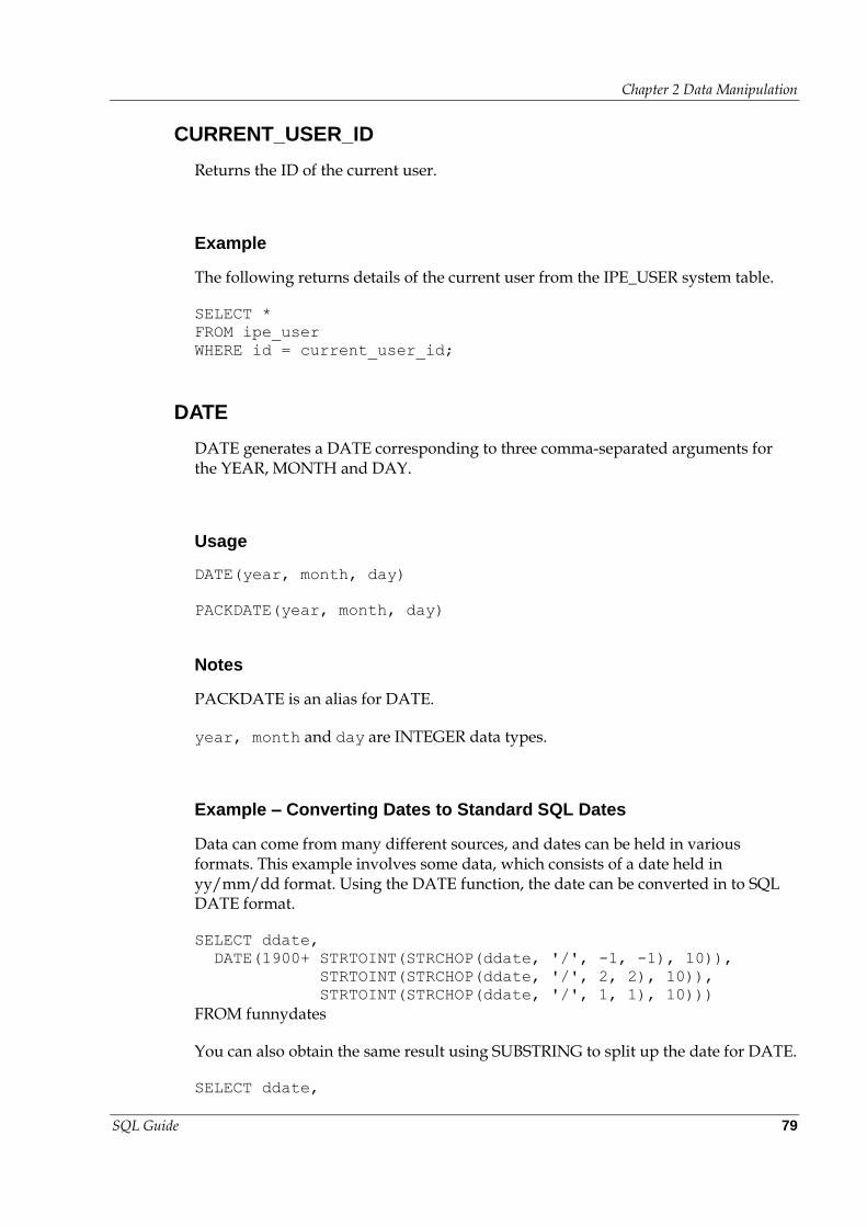
Chapter 2 Data Manipulation
SQL Guide 79
CURRENT_USER_ID
Returns the ID of the current user.
Example
The following returns details of the current user from the IPE_USER system table.
SELECT *
FROM ipe_user
WHERE id = current_user_id;
DATE
DATE generates a DATE corresponding to three comma-separated arguments for the YEAR, MONTH and DAY.
Usage
DATE(year, month, day)
PACKDATE(year, month, day)
Notes
PACKDATE is an alias for DATE.
year, month and day are INTEGER data types.
Example – Converting Dates to Standard SQL Dates
Data can come from many different sources, and dates can be held in various formats. This example involves some data, which consists of a date held in yy/mm/dd format. Using the DATE function, the date can be converted in to SQL DATE format.
SELECT ddate,
DATE(1900+ STRTOINT(STRCHOP(ddate, '/', -1, -1), 10)),
STRTOINT(STRCHOP(ddate, '/', 2, 2), 10)),
STRTOINT(STRCHOP(ddate, '/', 1, 1), 10)))
FROM funnydates
You can also obtain the same result using SUBSTRING to split up the date for DATE.
SELECT ddate,
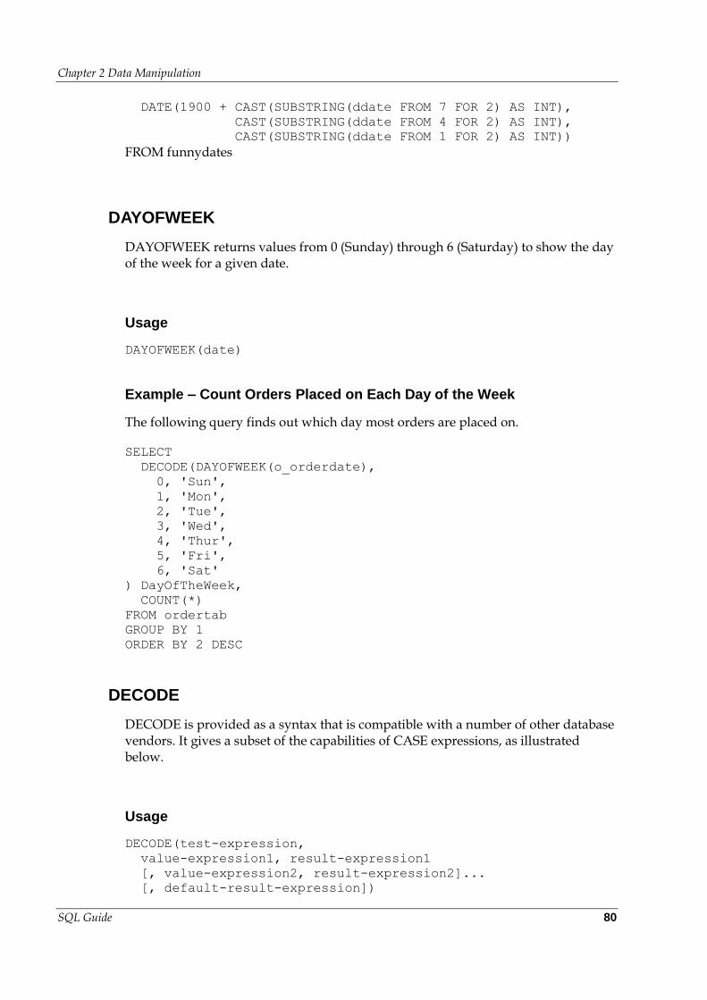
Chapter 2 Data Manipulation
SQL Guide 80
DATE(1900 + CAST(SUBSTRING(ddate FROM 7 FOR 2) AS INT),
CAST(SUBSTRING(ddate FROM 4 FOR 2) AS INT),
CAST(SUBSTRING(ddate FROM 1 FOR 2) AS INT))
FROM funnydates
DAYOFWEEK
DAYOFWEEK returns values from 0 (Sunday) through 6 (Saturday) to show the day of the week for a given date.
Usage
DAYOFWEEK(date)
Example – Count Orders Placed on Each Day of the Week
The following query finds out which day most orders are placed on.
SELECT
DECODE(DAYOFWEEK(o_orderdate),
0, 'Sun',
1, 'Mon',
2, 'Tue',
3, 'Wed',
4, 'Thur',
5, 'Fri',
6, 'Sat'
) DayOfTheWeek,
COUNT(*)
FROM ordertab
GROUP BY 1
ORDER BY 2 DESC
DECODE
DECODE is provided as a syntax that is compatible with a number of other database vendors. It gives a subset of the capabilities of CASE expressions, as illustrated below.
Usage
DECODE(test-expression,
value-expression1, result-expression1
[, value-expression2, result-expression2]...
[, default-result-expression])
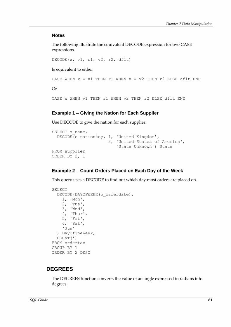
Chapter 2 Data Manipulation
SQL Guide 81
Notes
The following illustrate the equivalent DECODE expression for two CASE expressions.
DECODE(x, v1, r1, v2, r2, dflt)
Is equivalent to either
CASE WHEN x = v1 THEN r1 WHEN x = v2 THEN r2 ELSE dflt END
Or
CASE x WHEN v1 THEN r1 WHEN v2 THEN r2 ELSE dflt END
Example 1 – Giving the Nation for Each Supplier
Use DECODE to give the nation for each supplier.
SELECT s_name,
DECODE(s_nationkey, 1, 'United Kingdom',
2, 'United States of America',
'State Unknown') State
FROM supplier
ORDER BY 2, 1
Example 2 – Count Orders Placed on Each Day of the Week
This query uses a DECODE to find out which day most orders are placed on.
SELECT
DECODE(DAYOFWEEK(o_orderdate),
1, 'Mon',
2, 'Tue',
3, 'Wed',
4, 'Thur',
5, 'Fri',
6, 'Sat',
'Sun'
) DayOfTheWeek,
COUNT(*)
FROM ordertab
GROUP BY 1
ORDER BY 2 DESC
DEGREES
The DEGREES function converts the value of an angle expressed in radians into degrees.
Chapter 2 Data Manipulation
SQL Guide 82
Usage
DEGREES(argument)
Notes
The argument must be NUMERIC. An error occurs if the argument has an invalid data type, or if the result is too large to be represented by a FLOAT.
The value is calculated as DEGREES(x) = x * 180 / PI()
ERRORCODE
ERRORCODE returns the string associated with an error number.
Usage
ERRORCODE(error-number)
Notes
ERRORCODE is intended to help users query the Kognitio system tables.
Example
Select any rows associated with Disk Store status codes from the IPE_COMMAND table.
SELECT * FROM ipe_command WHERE errorcode(status) LIKE 'DS%'
ERRORNUM
ERRORNUM returns the number associated with an error code.
Usage
ERRORNUM(error-code)
Notes
ERRORNUM is intended to help users query the Kognitio system tables.
Chapter 2 Data Manipulation
SQL Guide 83
The error code passed in is NOT a string!
Example
Select any rows from the IPE_COMMAND table that have a status equivalent to the error code CI0100.
SELECT * FROM ipe_command WHERE status = errornum(CI0100)
EXP
The exponential function accepts any REAL number and returns the natural logarithm e raised to the x power.
Usage
EXP(argument)
Notes
The single argument for the EXP function must be NUMERIC (not an INTERVAL). The result has a FLOAT data type and is calculated by evaluating e (2.71828… — the natural logarithm base) raised to the power of the argument. You can obtain the value of ‘e’ itself by evaluating EXP(1).
An error occurs if the argument has an invalid data type, a negative value, or if the result is too large to be represented by a FLOAT. The latter occurs if the argument is above (approx.) 709.78.
EXTRACT
Use this function to return an INTEGER value for an individual field from a specified date-time.
Usage
EXTRACT(field FROM scalar-expression)
Chapter 2 Data Manipulation
SQL Guide 84
Notes
field is one of the following: YEAR, MONTH, DAY, HOUR, MINUTE, SECOND, TIMEZONE_HOUR or TIMEZONE_MINUTE.
scalar-expression is either a date-time expression or an interval expression.
EXTRACT returns the value field with data type exact numeric. This means that if you extract SECOND from 01:02:03.4, you get ‘3’.
Example 1 – Simple Extracts
Use EXTRACT to obtain the details of the month when each order was placed, and the month for delivery from the ORDERTAB table.
SELECT o_orderkey,
EXTRACT(MONTH FROM o_orderdate) month_ordered,
EXTRACT(MONTH FROM o_deliverytime) month_delivered
FROM ordertab
ORDER BY 1
The following queries analyses the months when orders are placed and the times of orders.
SELECT EXTRACT(MONTH FROM o_orderdate) mth, COUNT(*)
FROM ordertab
GROUP BY 1
ORDER BY 2 DESC
SELECT EXTRACT(HOUR FROM o_ordertime) hr, COUNT(*)
FROM ordertab
GROUP BY 1
ORDER BY hr
Example 2 – Using Extract to reformat dates
Use the EXTRACT function (combined with CAST and CONCATENATION) to retrieve date and month details for deliveries and reformat them in the form mm/yyyy, e.g. '12/1998'.
SELECT o_custkey,
CAST(EXTRACT(month FROM o_deliverytime) AS CHAR(2))
|| '/' ||
CAST(EXTRACT(YEAR FROM o_deliverytime) AS CHAR(4)) mmyyyy
FROM ordertab
ORDER BY 1, 2
Chapter 2 Data Manipulation
SQL Guide 85
FACTORIAL
Computes the factorial of the supplied argument. The factorial of a number N is the product of all the whole numbers between 1 and N.
Usage
FACTORIAL(argument)
Notes
The FACTORIAL function is calculated as GAMMA(argument + 1). Thus the same restrictions apply as for the GAMMA function, except the argument cannot be greater than 170.
FLOOR
Returns the greatest INTEGER <= the supplied argument.
Usage
FLOOR(argument)
Notes
The single argument for the FLOOR function must be NUMERIC. The result is the greatest INTEGER less than or equal to the argument. An error occurs if the argument has an invalid data type, or if the FLOOR cannot be represented in the same data type as the argument.
GAMMA
The GAMMA function is useful for statistical purposes in the same area as FACTORIAL(), except that it applies to non-INTEGERS as well.
Usage
GAMMA(argument)
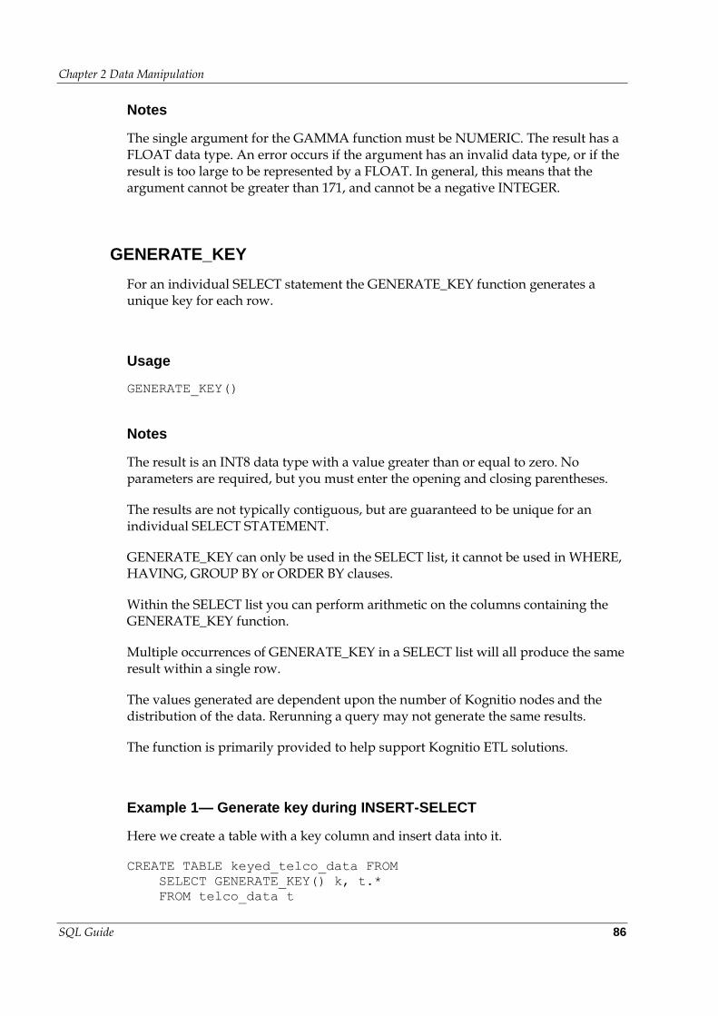
Chapter 2 Data Manipulation
SQL Guide 86
Notes
The single argument for the GAMMA function must be NUMERIC. The result has a FLOAT data type. An error occurs if the argument has an invalid data type, or if the result is too large to be represented by a FLOAT. In general, this means that the argument cannot be greater than 171, and cannot be a negative INTEGER.
GENERATE_KEY
For an individual SELECT statement the GENERATE_KEY function generates a unique key for each row.
Usage
GENERATE_KEY()
Notes
The result is an INT8 data type with a value greater than or equal to zero. No parameters are required, but you must enter the opening and closing parentheses.
The results are not typically contiguous, but are guaranteed to be unique for an individual SELECT STATEMENT.
GENERATE_KEY can only be used in the SELECT list, it cannot be used in WHERE, HAVING, GROUP BY or ORDER BY clauses.
Within the SELECT list you can perform arithmetic on the columns containing the GENERATE_KEY function.
Multiple occurrences of GENERATE_KEY in a SELECT list will all produce the same result within a single row.
The values generated are dependent upon the number of Kognitio nodes and the distribution of the data. Rerunning a query may not generate the same results.
The function is primarily provided to help support Kognitio ETL solutions.
Example 1— Generate key during INSERT-SELECT
Here we create a table with a key column and insert data into it.
CREATE TABLE keyed_telco_data FROM
SELECT GENERATE_KEY() k, t.*
FROM telco_data t
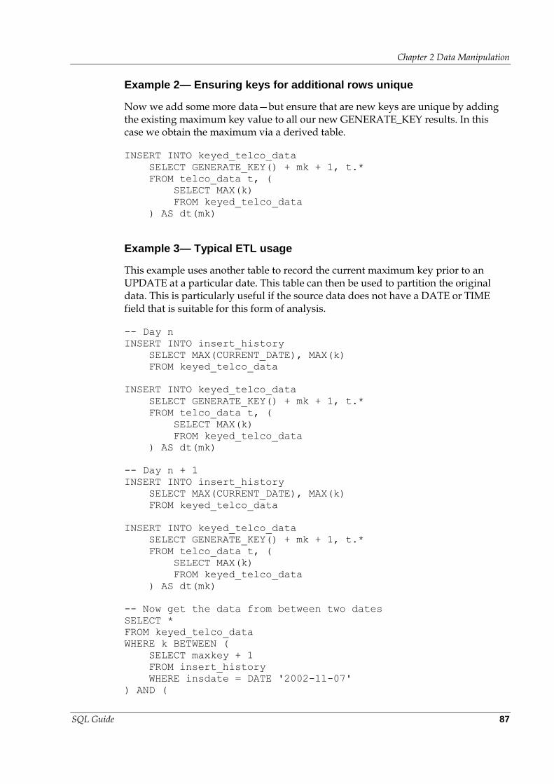
Chapter 2 Data Manipulation
SQL Guide 87
Example 2— Ensuring keys for additional rows unique
Now we add some more data—but ensure that are new keys are unique by adding the existing maximum key value to all our new GENERATE_KEY results. In this case we obtain the maximum via a derived table.
INSERT INTO keyed_telco_data
SELECT GENERATE_KEY() + mk + 1, t.*
FROM telco_data t, (
SELECT MAX(k)
FROM keyed_telco_data
) AS dt(mk)
Example 3— Typical ETL usage
This example uses another table to record the current maximum key prior to an UPDATE at a particular date. This table can then be used to partition the original data. This is particularly useful if the source data does not have a DATE or TIME field that is suitable for this form of analysis.
-- Day n
INSERT INTO insert_history
SELECT MAX(CURRENT_DATE), MAX(k)
FROM keyed_telco_data
INSERT INTO keyed_telco_data
SELECT GENERATE_KEY() + mk + 1, t.*
FROM telco_data t, (
SELECT MAX(k)
FROM keyed_telco_data
) AS dt(mk)
-- Day n + 1
INSERT INTO insert_history
SELECT MAX(CURRENT_DATE), MAX(k)
FROM keyed_telco_data
INSERT INTO keyed_telco_data
SELECT GENERATE_KEY() + mk + 1, t.*
FROM telco_data t, (
SELECT MAX(k)
FROM keyed_telco_data
) AS dt(mk)
-- Now get the data from between two dates
SELECT *
FROM keyed_telco_data
WHERE k BETWEEN (
SELECT maxkey + 1
FROM insert_history
WHERE insdate = DATE '2002-11-07'
) AND (
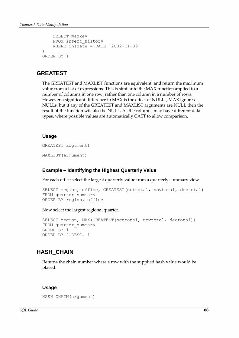
Chapter 2 Data Manipulation
SQL Guide 88
SELECT maxkey
FROM insert_history
WHERE insdate = DATE '2002-11-09'
)
ORDER BY 1
GREATEST
The GREATEST and MAXLIST functions are equivalent, and return the maximum value from a list of expressions. This is similar to the MAX function applied to a number of columns in one row, rather than one column in a number of rows. However a significant difference to MAX is the effect of NULLs; MAX ignores NULLs, but if any of the GREATEST and MAXLIST arguments are NULL then the result of the function will also be NULL. As the columns may have different data types, where possible values are automatically CAST to allow comparison.
Usage
GREATEST(argument)
MAXLIST(argument)
Example – Identifying the Highest Quarterly Value
For each office select the largest quarterly value from a quarterly summary view.
SELECT region, office, GREATEST(octtotal, novtotal, dectotal)
FROM quarter_summary
ORDER BY region, office
Now select the largest regional quarter.
SELECT region, MAX(GREATEST(octtotal, novtotal, dectotal))
FROM quarter_summary
GROUP BY 1
ORDER BY 2 DESC, 1
HASH_CHAIN
Returns the chain number where a row with the supplied hash value would be placed.
Usage
HASH_CHAIN(argument)
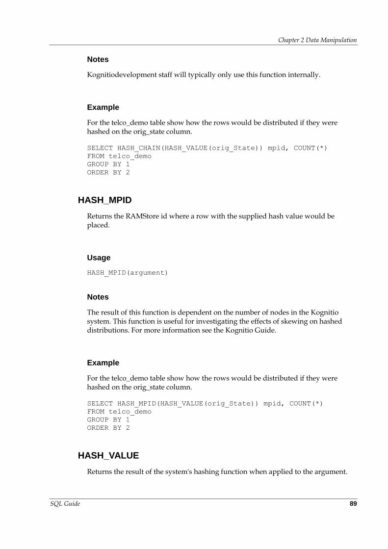
Chapter 2 Data Manipulation
SQL Guide 89
Notes
Kognitiodevelopment staff will typically only use this function internally.
Example
For the telco_demo table show how the rows would be distributed if they were hashed on the orig_state column.
SELECT HASH_CHAIN(HASH_VALUE(orig_State)) mpid, COUNT(*)
FROM telco_demo
GROUP BY 1
ORDER BY 2
HASH_MPID
Returns the RAMStore id where a row with the supplied hash value would be placed.
Usage
HASH_MPID(argument)
Notes
The result of this function is dependent on the number of nodes in the Kognitio system. This function is useful for investigating the effects of skewing on hashed distributions. For more information see the Kognitio Guide.
Example
For the telco_demo table show how the rows would be distributed if they were hashed on the orig_state column.
SELECT HASH_MPID(HASH_VALUE(orig_State)) mpid, COUNT(*)
FROM telco_demo
GROUP BY 1
ORDER BY 2
HASH_VALUE
Returns the result of the system's hashing function when applied to the argument.
Chapter 2 Data Manipulation
SQL Guide 90
Usage
HASH_VALUE(argument)
Notes
For any given argument this function returns the same value, regardless of the number of nodes in the Kognitio system. This function is useful for investigating the effects of skewing on hashed distributions. For more information see the Kognitio Guide.
Example
For the telco_demo table return all the possible HASH_VALUES or the orig_state column and count how many rows return each value.
SELECT HASH_VALUE(orig_State), COUNT(*)
FROM telco_demo
GROUP BY 1
ORDER BY 2
IMAGE_ID
The IMAGE_ID function is useful for querying system tables.
Usage
IMAGE_ID(image)
Notes
The argument is an unquoted string that specifies the image name; it can include the schema name and separator.
Example
The following query can be used to determine the distribution of a particular view image:
SELECT distribution FROM ipe_allview_img
WHERE image_id = IMAGE_ID(CUSTOMER_VIEW)
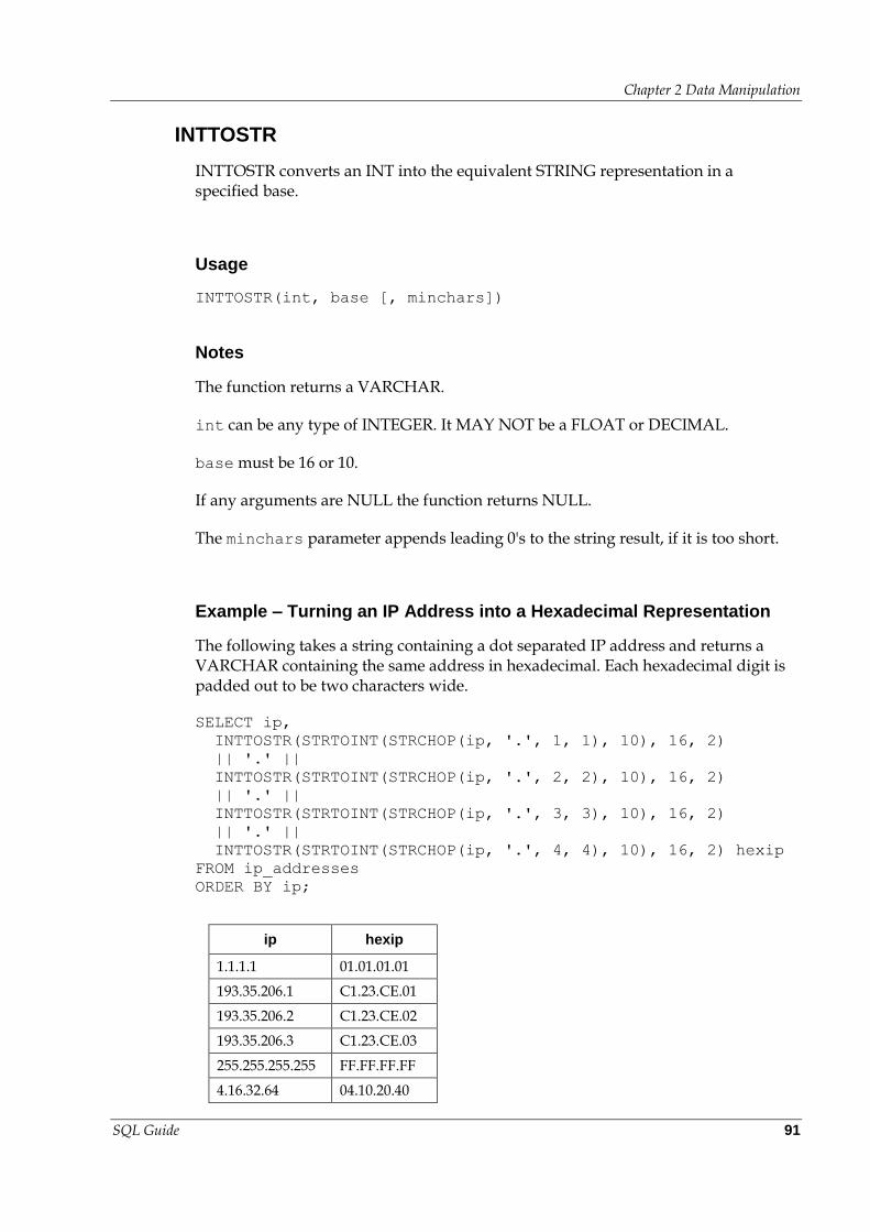
Chapter 2 Data Manipulation
SQL Guide 91
INTTOSTR
INTTOSTR converts an INT into the equivalent STRING representation in a specified base.
Usage
INTTOSTR(int, base [, minchars])
Notes
The function returns a VARCHAR.
int can be any type of INTEGER. It MAY NOT be a FLOAT or DECIMAL.
base must be 16 or 10.
If any arguments are NULL the function returns NULL.
The minchars parameter appends leading 0's to the string result, if it is too short.
Example – Turning an IP Address into a Hexadecimal Representation
The following takes a string containing a dot separated IP address and returns a VARCHAR containing the same address in hexadecimal. Each hexadecimal digit is padded out to be two characters wide.
SELECT ip,
INTTOSTR(STRTOINT(STRCHOP(ip, '.', 1, 1), 10), 16, 2)
|| '.' ||
INTTOSTR(STRTOINT(STRCHOP(ip, '.', 2, 2), 10), 16, 2)
|| '.' ||
INTTOSTR(STRTOINT(STRCHOP(ip, '.', 3, 3), 10), 16, 2)
|| '.' ||
INTTOSTR(STRTOINT(STRCHOP(ip, '.', 4, 4), 10), 16, 2) hexip
FROM ip_addresses
ORDER BY ip;
ip hexip
1.1.1.1 01.01.01.01
193.35.206.1 C1.23.CE.01
193.35.206.2 C1.23.CE.02
193.35.206.3 C1.23.CE.03
255.255.255.255 FF.FF.FF.FF
4.16.32.64 04.10.20.40
Chapter 2 Data Manipulation
SQL Guide 92
LEAST
The LEAST and MINLIST functions are equivalent and return the minimum value from a list of expressions. This is similar to the MIN function applied to a number of columns in one row, rather than one column in a number of rows. However a significant difference to MIN is the effect of NULLs; MIN ignores NULLs, but if any of the LEAST and MINLIST arguments are NULL then the result of the function will also be NULL. As the columns may have different data types, where possible values are automatically CAST to allow comparison.
Usage
LEAST(argument)
MINLIST(argument)
Example – Identifying the Smallest Quarterly Value
For each office select the smallest quarterly value from a quarterly summary view.
SELECT region, office, LEAST(octtotal, novtotal, dectotal)
FROM quarter_summary
ORDER BY region, office
Now select the smallest regional quarter.
SELECT region, MIN(LEAST(octtotal, novtotal, dectotal))
FROM quarter_summary
GROUP BY 1
ORDER BY 2 DESC, 1
LEFT
Use the LEFT function to obtain a substring consisting of the left part of a character string with the specified number of characters.
Usage
LEFT(string, len)
Notes
LEFT can only be used with character strings.
len must be a positive integer that specifies how many characters of string will be returned. If len is negative, an error is returned.
Chapter 2 Data Manipulation
SQL Guide 93
Example 1 – Incoming Postcode
Using the CUSTOMER table, create a view with a column called postcode_start (CHAR(4)), containing the first 4 digits only from the postcode column (CHAR(8)). The shortened postcode is useful for analyzing by postal district.
CREATE VIEW inward_postcode(name, address, postcode) AS
SELECT c_name, c_address, LEFT(c_postcode, 4)
FROM customer
Example 2 – Extracting House Numbers from an Address
In the CUSTOMER table, many addresses have a house number. The following returns the house number as a separate column.
SELECT c_name, c_address AS fulladd,
CAST(
LEFT(c_address, POSITION(' ' IN c_address) – 1)
AS INT) AS number
FROM customer
WHERE c_address MATCHING '^[0-9]+ +'
ORDER BY 3
LOG10
The LOG10 Function returns the base 10 logarithm of the supplied argument.
Usage
LOG10(argument)
Notes
The single argument for the LOG10 function must have a NUMERIC data type (but not an INTERVAL). The result has a FLOAT data type.
An error occurs if the argument has an invalid data type or is negative.
LOWER
Use the LOWER function to convert a given string to lower case.
Chapter 2 Data Manipulation
SQL Guide 94
Usage
LOWER(string)
Notes
LOWER can only be used to convert character strings.
Example
This example obtains details of all the Smalltown suppliers without an ST1 postcode. Here, LOWER is used before s_address in the first WHERE condition, so that LIKE ‘%smalltown%’ can match addresses entered as ‘smalltown’, ‘Smalltown’ or ‘SMALLTOWN’. UPPER is used with the second WHERE condition, to ensure the LIKE condition (‘ST1 %') matches all occurrences of ST1, regardless of case.
SELECT *
FROM supplier
WHERE LOWER(s_address) LIKE '%smalltown%' AND
UPPER(s_address) NOT LIKE 'ST1 %'
ORDER BY s_suppkey
LN
The LN Function returns the natural logarithm for the supplied argument.
Usage
LN(argument)
Notes
The single argument for the LN function has a NUMERIC data type (not an INTERVAL). The result has a FLOAT data type.
An error occurs if the argument has an invalid data type or if the argument is negative.
LPAD
LPAD left pads a string to a given width with a specified character.
Chapter 2 Data Manipulation
SQL Guide 95
Usage
LPAD(string, width, [character])
Notes
string can be a CHAR or VARCHAR data type, note that any trailing spaces are not automatically removed from a CHAR data types. width can be any INTEGER constant or expression. character can be any single character, the default value is a space. The function has no effect if string is already at least width characters wide.
Examples
The following SQL formats entries in a report. It makes the first integer column six digits wide by prefixing with zeros; the second, decimal column is padded to always have five digits to the left of the decimal point, but the sign is maintained; padding left and right with hyphens centers the final column.
SELECT LPAD(CAST(orderkey AS VARCHAR), 6, '0') AS okey,
DECODE(SIGN(o_totalprice), -1, '-', ' ') ||
LPAD(CAST(ABS(o_totalprice) AS VARCHAR), 8, '0') AS oprice,
LPAD(
RPAD(TRIM(o_orderpriority), 12, '-'),
17, '-') AS opriority
FROM ordertab
ORDER BY 1
The following SQL makes use of an expression to format entries in a report so that all entries are padded with a hyphen to make them the same width of the widest entry.
SELECT LPAD(CAST(c_name AS VARCHAR), maxl, '-')
FROM customer,
(SELECT MAX(CHAR_LENGTH(CAST(c_name AS VARCHAR)))
FROM customer) AS dt(maxl)
ORDER BY 1;
MAXLIST
See GREATEST.
MINLIST
See LEAST
Chapter 2 Data Manipulation
SQL Guide 96
MOD
The MOD function returns the modulus for a pair of values.
Usage
MOD(value, divisor)
Notes
MOD(A, B) results in the remainder when A is divided by B.
NULLIF
The NULLIF function provides shorthand for a commonly used instance of CASE. It provides a simple way to return NULL as a replacement for a particular value.
Usage
NULLIF(value-expression1, value-expression2)
The above is equivalent to the following CASE expression.
CASE
WHEN value-expression1 = value-expression2
THEN NULL
ELSE value-expression1
END
Example 1 – Replace a value with NULL
Suppose that Petes Parts has ceased trading. Use NULLIF to replace the name with NULL, when you select from the SUPPLIER table.
SELECT s_suppkey, NULLIF(s_name, 'Petes parts')
FROM supplier
ORDER BY 1
Example 2 – Removing values from aggregates
Because NULLs are ignored when aggregates are calculated, NULLIF can be used to eliminate certain values from COUNTs, SUMs, etc. The following SQL excludes from a count orders placed on a certain date.
Chapter 2 Data Manipulation
SQL Guide 97
SELECT
COUNT(o_orderdate) AS allorders,
COUNT(NULLIF(o_orderdate, DATE '1998-10-14')) AS exc141098
FROM ordertab;
NVL
NVL is a synonym for COALESCE. See COALESCE.
OCTET_LENGTH
Use the OCTET_LENGTH function to find the length of a particular string in bytes.
Usage
SELECT OCTET_LENGTH(string)
Notes
You can only use the OCTET_LENGTH function to measure character strings.
As Kognitio can store national characters based on the syntax extensions to SQL:1999, which use Unicode and ISO standards it is possible for the length of a string measured in characters to be different to the length measured in bytes.
OVERLAY
Use the OVERLAY function to replace a substring with another substring.
Usage
OVERLAY(string1 PLACING string2 FROM start [FOR length])
Notes
The OVERLAY function returns a string where a substring of length, beginning at start has been deleted from string1, and where string2 has been inserted into string1 beginning at start. If the value of start plus length is greater than the length of string1, the substring that is deleted is from start to the end of string1.
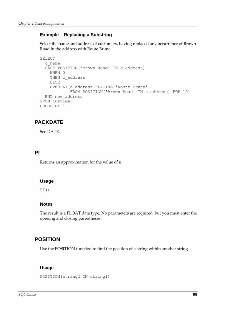
Chapter 2 Data Manipulation
SQL Guide 98
Example – Replacing a Substring
Select the name and address of customers, having replaced any occurrence of Brown Road in the address with Route Brune.
SELECT
c_name,
CASE POSITION('Brown Road' IN c_address)
WHEN 0
THEN c_address
ELSE
OVERLAY(c_address PLACING 'Route Brune'
FROM POSITION('Brown Road' IN c_address) FOR 10)
END new_address
FROM customer
ORDER BY 1
PACKDATE
See DATE.
PI
Returns an approximation for the value of π
Usage
PI()
Notes
The result is a FLOAT data type. No parameters are required, but you must enter the opening and closing parentheses.
POSITION
Use the POSITION function to find the position of a string within another string.
Usage
POSITION(string2 IN string1)
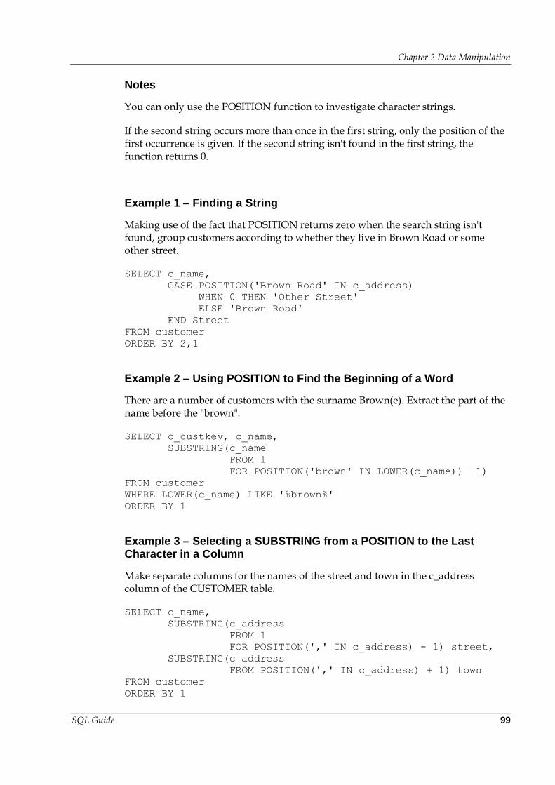
Chapter 2 Data Manipulation
SQL Guide 99
Notes
You can only use the POSITION function to investigate character strings.
If the second string occurs more than once in the first string, only the position of the first occurrence is given. If the second string isn't found in the first string, the function returns 0.
Example 1 – Finding a String
Making use of the fact that POSITION returns zero when the search string isn't found, group customers according to whether they live in Brown Road or some other street.
SELECT c_name,
CASE POSITION('Brown Road' IN c_address)
WHEN 0 THEN 'Other Street'
ELSE 'Brown Road'
END Street
FROM customer
ORDER BY 2,1
Example 2 – Using POSITION to Find the Beginning of a Word
There are a number of customers with the surname Brown(e). Extract the part of the name before the "brown".
SELECT c_custkey, c_name,
SUBSTRING(c_name
FROM 1
FOR POSITION('brown' IN LOWER(c_name)) –1)
FROM customer
WHERE LOWER(c_name) LIKE '%brown%'
ORDER BY 1
Example 3 – Selecting a SUBSTRING from a POSITION to the Last Character in a Column
Make separate columns for the names of the street and town in the c_address column of the CUSTOMER table.
SELECT c_name,
SUBSTRING(c_address
FROM 1
FOR POSITION(',' IN c_address) - 1) street,
SUBSTRING(c_address
FROM POSITION(',' IN c_address) + 1) town
FROM customer
ORDER BY 1
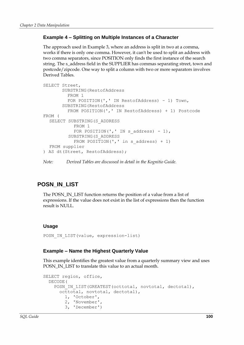
Chapter 2 Data Manipulation
SQL Guide 100
Example 4 – Splitting on Multiple Instances of a Character
The approach used in Example 3, where an address is split in two at a comma, works if there is only one comma. However, it can't be used to split an address with two comma separators, since POSITION only finds the first instance of the search string. The s_address field in the SUPPLIER has commas separating street, town and postcode/zipcode. One way to split a column with two or more separators involves Derived Tables.
SELECT Street,
SUBSTRING(RestofAddress
FROM 1
FOR POSITION(',' IN RestofAddress) - 1) Town,
SUBSTRING(RestofAddress
FROM POSITION(',' IN RestofAddress) + 1) Postcode
FROM (
SELECT SUBSTRING(S_ADDRESS
FROM 1
FOR POSITION(',' IN s_address) - 1),
SUBSTRING(S_ADDRESS
FROM POSITION(',' in s_address) + 1)
FROM supplier
) AS dt(Street, RestofAddress);
Note: Derived Tables are discussed in detail in the Kognitio Guide.
POSN_IN_LIST
The POSN_IN_LIST function returns the position of a value from a list of expressions. If the value does not exist in the list of expressions then the function result is NULL.
Usage
POSN_IN_LIST(value, expression-list)
Example – Name the Highest Quarterly Value
This example identifies the greatest value from a quarterly summary view and uses POSN_IN_LIST to translate this value to an actual month.
SELECT region, office,
DECODE(
POSN_IN_LIST(GREATEST(octtotal, novtotal, dectotal),
octtotal, novtotal, dectotal),
1, 'October',
2, 'November',
3, 'December')
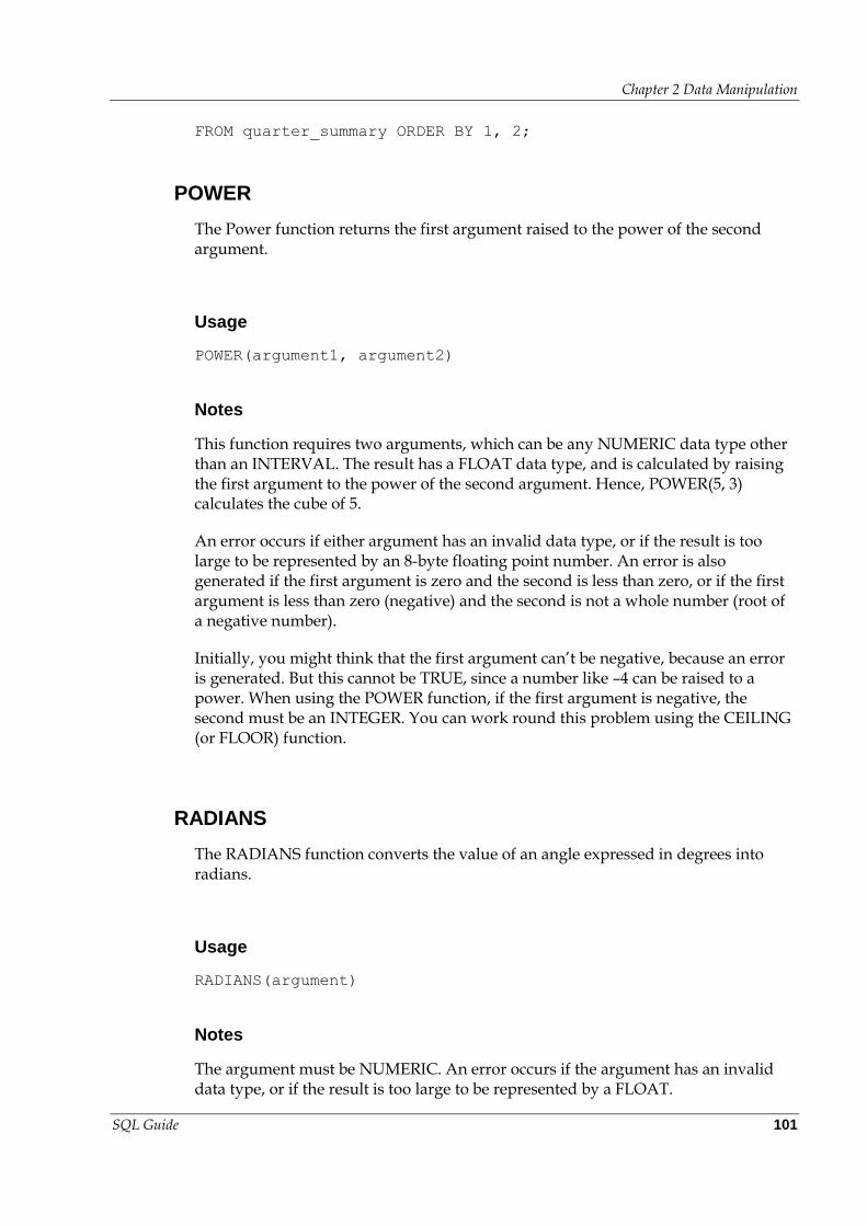
Chapter 2 Data Manipulation
SQL Guide 101
FROM quarter_summary ORDER BY 1, 2;
POWER
The Power function returns the first argument raised to the power of the second argument.
Usage
POWER(argument1, argument2)
Notes
This function requires two arguments, which can be any NUMERIC data type other than an INTERVAL. The result has a FLOAT data type, and is calculated by raising the first argument to the power of the second argument. Hence, POWER(5, 3) calculates the cube of 5.
An error occurs if either argument has an invalid data type, or if the result is too large to be represented by an 8-byte floating point number. An error is also generated if the first argument is zero and the second is less than zero, or if the first argument is less than zero (negative) and the second is not a whole number (root of a negative number).
Initially, you might think that the first argument can’t be negative, because an error is generated. But this cannot be TRUE, since a number like –4 can be raised to a power. When using the POWER function, if the first argument is negative, the second must be an INTEGER. You can work round this problem using the CEILING (or FLOOR) function.
RADIANS
The RADIANS function converts the value of an angle expressed in degrees into radians.
Usage
RADIANS(argument)
Notes
The argument must be NUMERIC. An error occurs if the argument has an invalid data type, or if the result is too large to be represented by a FLOAT.
Chapter 2 Data Manipulation
SQL Guide 102
The value is calculated as RADIANS(x) = x * PI() / 180
RIGHT
Use the RIGHT function to obtain a substring consisting of the right part of a character string with the specified number of characters.
Usage
RIGHT(string, len)
Notes
RIGHT can only be used with character strings.
len must be a positive integer that specifies how many characters of string will be returned. If len is negative, an error is returned.
Example 1 – Outgoing Postcode
You can select the last three characters of a UK postcode, which form the “outgoing” part. These are useful for surveys based on a single postal district.
CREATE VIEW outward_postcode(name, address, postcode) AS
SELECT c_name, c_address, RIGHT(c_postcode, 3)
FROM customer
Example 2 – Zipcode
In the SUPPLIER table addresses for US suppliers end with a 5-digit zip code followed by a full stop. Return the zip code as a separate column.
SELECT s_name, s_address,
TRIM(TRAILING '.' FROM RIGHT(s_address, 6)) AS zipcode
FROM supplier
WHERE s_nationkey = 2
RPAD
RPAD right pads a string to a given width with a specified character.
Chapter 2 Data Manipulation
SQL Guide 103
Usage
RPAD(string, width, [character])
Notes
string can be a CHAR or VARCHAR data type, note that any trailing spaces are not automatically removed from a CHAR data types. width can be any INTEGER constant or expression. character can be any single character, the default value is a space. The function has no effect if string is already at least width characters wide.
Examples
The following SQL formats entries in a report. It makes the first integer column six digits wide by prefixing with zeros; the second, decimal column is padded to always have five digits to the left of the decimal point, but the sign is maintained; padding left and right with hyphens centers the final column.
SELECT LPAD(CAST(orderkey AS VARCHAR), 6, '0') AS okey,
DECODE(SIGN(o_totalprice), -1, '-', ' ') ||
LPAD(CAST(ABS(o_totalprice) AS VARCHAR), 8, '0') AS oprice,
LPAD(
RPAD(TRIM(o_orderpriority), 12, '-'),
17, '-') AS opriority
FROM ordertab
ORDER BY 1
The following SQL makes use of an expression to format entries in a report so that all entries are padded with a hyphen to make them the same width of the widest entry.
SELECT RPAD(CAST(c_name AS VARCHAR), maxl, '-')
FROM customer,
(SELECT MAX(CHAR_LENGTH(CAST(c_name AS VARCHAR)))
FROM customer) AS dt(maxl)
ORDER BY 1;
SCHEMA_ID
The SCHEMA_ID function is useful for querying system tables.
Usage
SCHEMA_ID(schema)
Chapter 2 Data Manipulation
SQL Guide 104
Notes
The argument is an unquoted string that specifies the schema name.
Example
Previously a query of the following form had to be used when a reference to the ID of a schema was required:
SELECT COUNT(*) FROM ipe_table
WHERE schema_id = (
SELECT id FROM ipe_schema WHERE name = 'POC')
This query can now be written as:
SELECT COUNT(*) FROM ipe_table
WHERE schema_id = SCHEMA_ID(POC)
SIGN
The SIGN function indicates the sign of the supplied argument.
Usage
SIGN(argument)
Notes
The single argument for the SIGN function must be either NUMERIC or an INTERVAL. The result is a 1-byte INTEGER; ‘-1’ if the argument was less than zero, ‘1’ if the argument is greater than zero, or ‘0’ if the argument is zero. An error occurs if the argument has an invalid data type.
Example – Padding Output Numbers
This query outputs numbers with fixed width and padding with 0s, while maintaining the sign, which can be useful in reports.
SELECT
CAST(CASE SIGN(i)
WHEN -1 THEN '-'
ELSE ''
END AS VARCHAR) ||
SUBSTRING('000000'
FROM 1
Chapter 2 Data Manipulation
SQL Guide 105
FOR 6 - CHAR_LENGTH(CAST(i AS VARCHAR))) ||
CAST(ABS(i) AS VARCHAR) AS newi
FROM num
ORDER BY 1
Note: If the number is not negative we prefix with a NULL string, which we need to CAST to VARCHAR to prevent the NULL becoming a CHAR(1) and making the minus 'hang' to the left.
The Kognitio Plugin function to_char can be used to perform a variety of output formatting, including the above in a straightforward way.
SIN
SIN calculates the sine for the specified argument.
Usage
SIN(argument)
Notes
The argument must be NUMERIC. An error occurs if the argument has an invalid data type, or if the result is too large to be represented by a FLOAT.
SINH
SINH calculates the hyperbolic sine for the specified argument.
Usage
SINH(argument)
Notes
The argument must be NUMERIC. An error occurs if the argument has an invalid data type, or if the result is too large to be represented by a FLOAT.
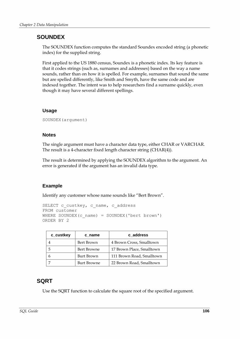
Chapter 2 Data Manipulation
SQL Guide 106
SOUNDEX
The SOUNDEX function computes the standard Soundex encoded string (a phonetic index) for the supplied string.
First applied to the US 1880 census, Soundex is a phonetic index. Its key feature is that it codes strings (such as, surnames and addresses) based on the way a name sounds, rather than on how it is spelled. For example, surnames that sound the same but are spelled differently, like Smith and Smyth, have the same code and are indexed together. The intent was to help researchers find a surname quickly, even though it may have several different spellings.
Usage
SOUNDEX(argument)
Notes
The single argument must have a character data type, either CHAR or VARCHAR. The result is a 4-character fixed length character string (CHAR(4)).
The result is determined by applying the SOUNDEX algorithm to the argument. An error is generated if the argument has an invalid data type.
Example
Identify any customer whose name sounds like “Bert Brown”.
SELECT c_custkey, c_name, c_address
FROM customer
WHERE SOUNDEX(c_name) = SOUNDEX('bert brown')
ORDER BY 2
c_custkey c_name c_address
4 Bert Brown 4 Brown Cross, Smalltown
5 Bert Browne 17 Brown Place, Smalltown
6 Burt Brown 111 Brown Road, Smalltown
7 Burt Browne 22 Brown Road, Smalltown
SQRT
Use the SQRT function to calculate the square root of the specified argument.
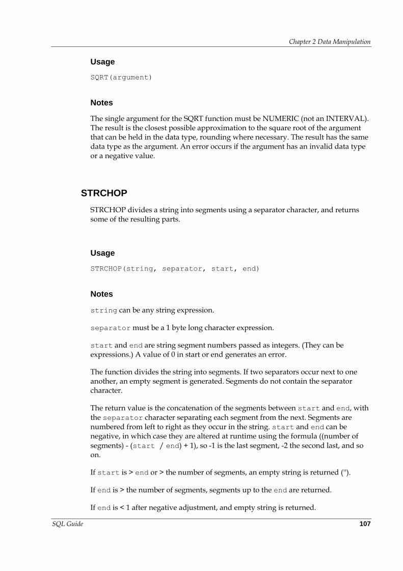
Chapter 2 Data Manipulation
SQL Guide 107
Usage
SQRT(argument)
Notes
The single argument for the SQRT function must be NUMERIC (not an INTERVAL). The result is the closest possible approximation to the square root of the argument that can be held in the data type, rounding where necessary. The result has the same data type as the argument. An error occurs if the argument has an invalid data type or a negative value.
STRCHOP
STRCHOP divides a string into segments using a separator character, and returns some of the resulting parts.
Usage
STRCHOP(string, separator, start, end)
Notes
string can be any string expression.
separator must be a 1 byte long character expression.
start and end are string segment numbers passed as integers. (They can be expressions.) A value of 0 in start or end generates an error.
The function divides the string into segments. If two separators occur next to one another, an empty segment is generated. Segments do not contain the separator character.
The return value is the concatenation of the segments between start and end, with the separator character separating each segment from the next. Segments are numbered from left to right as they occur in the string. start and end can be negative, in which case they are altered at runtime using the formula ((number of segments) - (start / end) + 1), so -1 is the last segment, -2 the second last, and so on.
If start is > end or > the number of segments, an empty string is returned ('').
If end is > the number of segments, segments up to the end are returned.
If end is < 1 after negative adjustment, and empty string is returned.
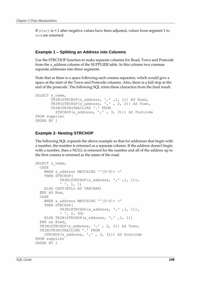
Chapter 2 Data Manipulation
SQL Guide 108
If start is < 1 after negative values have been adjusted, values from segment 1 to end are returned.
Example 1 – Splitting an Address into Columns
Use the STRCHOP function to make separate columns for Road, Town and Postcode from the s_address column of the SUPPLIER table. In this column two commas separate addresses into three segments.
Note that as there is a space following each comma separator, which would give a space at the start of the Town and Postcode columns. Also, there is a full stop at the end of the postcode. The following SQL trims these characters from the final result.
SELECT s_name,
TRIM(STRCHOP(s_address, ',' ,1, 1)) AS Road,
TRIM(STRCHOP(s_address, ',' , 2, 2)) AS Town,
TRIM(TRIM(TRAILING '.' FROM
STRCHOP(s_address, ',' , 3, 3))) AS Postcode
FROM supplier
ORDER BY 1
Example 2- Nesting STRCHOP
The following SQL expands the above example so that for addresses that begin with a number, the number is returned as a separate column. If the address doesn't begin with a number, then a NULL is returned for the number and all of the address up to the first comma is returned as the name of the road.
SELECT s_name,
CASE
WHEN s_address MATCHING '^[0-9]+ +'
THEN STRCHOP(
TRIM(STRCHOP(s_address, ',' ,1, 1)),
' ', 1, 1)
ELSE CAST(NULL AS VARCHAR)
END AS Num,
CASE
WHEN s_address MATCHING '^[0-9]+ +'
THEN STRCHOP(
TRIM(STRCHOP(s_address, ',' ,1, 1)),
' ', 2, 99)
ELSE TRIM(STRCHOP(s_address, ',' ,1, 1))
END as Road,
TRIM(STRCHOP(s_address, ',' , 2, 2)) AS Town,
TRIM(TRIM(TRAILING '.' FROM
STRCHOP(s_address, ',' , 3, 3))) AS Postcode
FROM supplier
ORDER BY 1
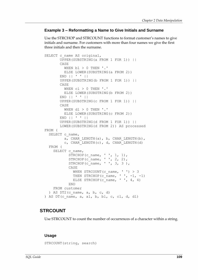
Chapter 2 Data Manipulation
SQL Guide 109
Example 3 – Reformatting a Name to Give Initials and Surname
Use the STRCHOP and STRCOUNT functions to format customer’s names to give initials and surname. For customers with more than four names we give the first three initials and then the surname.
SELECT c_name AS original,
UPPER(SUBSTRING(a FROM 1 FOR 1)) ||
CASE
WHEN bl > 0 THEN '.'
ELSE LOWER(SUBSTRING(a FROM 2))
END || ' ' ||
UPPER(SUBSTRING(b FROM 1 FOR 1)) ||
CASE
WHEN cl > 0 THEN '.'
ELSE LOWER(SUBSTRING(b FROM 2))
END || ' ' ||
UPPER(SUBSTRING(c FROM 1 FOR 1)) ||
CASE
WHEN dl > 0 THEN '.'
ELSE LOWER(SUBSTRING(c FROM 2))
END || ' ' ||
UPPER(SUBSTRING(d FROM 1 FOR 1)) ||
LOWER(SUBSTRING(d FROM 2)) AS processed
FROM (
SELECT c_name,
a, CHAR_LENGTH(a), b, CHAR_LENGTH(b),
c, CHAR_LENGTH(c), d, CHAR_LENGTH(d)
FROM (
SELECT c_name,
STRCHOP(c_name, ' ', 1, 1),
STRCHOP(c_name, ' ', 2, 2),
STRCHOP(c_name, ' ', 3, 3 ),
CASE
WHEN STRCOUNT(c_name, ' ') > 3
THEN STRCHOP(c_name, ' ', -1, -1)
ELSE STRCHOP(c_name, ' ', 4, 4)
END
FROM customer
) AS DT2(c_name, a, b, c, d)
) AS DT(c_name, a, al, b, bl, c, cl, d, dl)
STRCOUNT
Use STRCOUNT to count the number of occurrences of a character within a string.
Usage
STRCOUNT(string, search)
Chapter 2 Data Manipulation
SQL Guide 110
Notes
string can be any STRING expression. search can be any STRING expression, but must be of length 1.
The result is an INT4. The result is NULL if any argument is NULL.
Example 1 – Find the Number of Segments in a URL
Use STRCOUNT to determine the number of dot-separators in the URL for each supplier's website.
SELECT s_name,
s_url,
STRCOUNT(s_url, '.') AS No_Dots
FROM supplier
ORDER BY 3 DESC, 1
Example 2 – Find the Average Number of Words in Supplier Comments
Using STRCOUNT, find the average number of words in comments in the SUPPLIER table.
SELECT AVG(1 + STRCOUNT(s_comment, ' '))
FROM supplier
Note that this will return the average length as an INTEGER. However, if you change the literal value from 1 to 1.0, a DECIMAL will be returned, e.g.
SELECT AVG(1.0 + STRCOUNT(s_comment, ' '))
FROM supplier
STRPACKINTS
STRPACKINTS returns an INT8 containing the number made up of the sections of string.
Usage
STRPACKINTS(string, separator, bits, count, base)
Notes
The string arguments specify the value to pack.
Each segment is then treated as a string representation of a number with base base, and is converted into a number occupying bits bits.
Chapter 2 Data Manipulation
SQL Guide 111
There must not be more than count segments.
string must ONLY contains the character representations of numbers (0-9 for decimal, 0-9a-fA-F for hexadecimal). If the string is a CHAR this includes white space, so it is necessary to TRIM any trailing spaces, or alternately CAST the CHAR to a VARCHAR.
Example – Pack an IP Address into an INT8
Pack an IP address into an INT8.
SELECT ip, STRPACKINTS(ip, '.', 8, 4, 10) AS packedip
FROM IP_ADDRESSES
ORDER BY 1;
STRPOS
Use STRPOS to find the offset of a character within a string.
Usage
STRPOS(string, search[, occurrence])
Notes
string can be any string expression, search can be any string expression.
occurrence is an INTEGER, and is optional. The compiler assumes 1 if it isn't supplied, and it returns an error if occurrence is 0.
1 is the first occurrence from the start, 2 the second, and so on. Negative values count from the end; so -1 is the last occurrence, -2 the second last, and so on.
The return value is the offset within the string of the specified occurrence of search. 1 is the first character in the string. 0 is returned if the specified occurrence doesn't occur in the string. Note that trailing spaces are significant if search is a CHAR data type. NULL is returned if any argument is NULL.
It is possible for string to contain overlapping occurrences of search. Searching for an occurrence begins after the FIRST character of the previous occurrence, so overlapping occurrences generate multiple occurrence numbers.
Chapter 2 Data Manipulation
SQL Guide 112
Example 1 – Locating the Position of Dot-Separators in a URL
Use STRPOS to show the positions of each dot in a URL separator.
SELECT s_name, s_url,
STRPOS(s_url, '.' , 1),
STRPOS(s_url, '.' , 2),
STRPOS(s_url, '.' , 3)
FROM supplier
Example 2 – Locating the Last Separator in a String
If you have a negative value for occurrence, the position of the last occurrence of the search relative to the end of the string is returned. This is useful for locating the position of the last dot separator in a URL, given that the numbers of segments (and consequently the number of dots) vary.
The following query returns the positions of the last two dots in a URL.
SELECT s_name, s_url,
STRCOUNT(s_url, '.') AS No_Dots,
STRPOS(s_url, '.' , -2) AS SecondLastDot,
STRPOS(s_url, '.' , -1) AS LastDot
FROM supplier
ORDER BY 1
Example 3 – Using STRPOS In a WHERE Clause
Find customer addresses containing the string 'cross' in any case, using STRPOS. The position search will be greater than zero, if the string is present.
SELECT c_name, c_address
FROM customer
WHERE STRPOS(LOWER(c_address), 'cross') > 0
ORDER BY 1
STRTOINT
Usage STRTOINT converts a STRING representation of a number with a definable base to an INTEGER.
Usage
STRTOINT(string, base)
Chapter 2 Data Manipulation
SQL Guide 113
Notes
string is the string to convert, and can be any string expression. It may contain white space characters.
base is the is the base that the string is assumed to be in. It is numeric and must be either in the range 2-10, or 16.
The number represented must be an INTEGER (that is, there must be no decimal point). Overflow is returned if the converted value cannot fit into an INT8. An error is returned if the string cannot be converted because of an invalid format.
Example – Splitting an IP Address
The following SQL extracts the four numeric parts of an IP address and returns them as individual integers.
SELECT
ip,
STRTOINT(STRCHOP(ip, '.', 1, 1), 10) AS p1,
STRTOINT(STRCHOP(ip, '.', 2, 2), 10) AS p2,
STRTOINT(STRCHOP(ip, '.', 3, 3), 10) AS p3,
STRTOINT(STRCHOP(ip, '.', 4, 4), 10) AS p4
FROM ip_addresses
ORDER ip;
ip p1 p2 p3 p4
1.1.1.1 1 1 1 1
193.35.206.1 193 35 206 1
193.35.206.2 193 35 206 2
193.35.206.3 193 35 206 3
255.255.255.255 255 255 255 255
4.16.32.64 4 16 32 64
The following packs the IP address string into a single INT. Note extra work is required because INTs are signed data types and the IP address can be 32 bits in length.
SELECT ip,
CASE
WHEN ip8 > 2147483647
THEN CAST (-4294967296 + ip8 AS INT4)
ELSE CAST(ip8 AS INT4)
END AS ipint
FROM (
SELECT ip,
STRTOINT(STRCHOP(ip, '.', 1, 1), 10) * 256 * 256 * 256 +
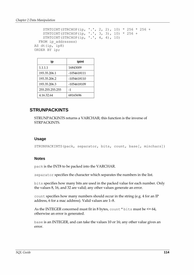
Chapter 2 Data Manipulation
SQL Guide 114
STRTOINT(STRCHOP(ip, '.', 2, 2), 10) * 256 * 256 +
STRTOINT(STRCHOP(ip, '.', 3, 3), 10) * 256 +
STRTOINT(STRCHOP(ip, '.', 4, 4), 10)
FROM ip_addresses)
AS dt(ip, ip8)
ORDER BY ip;
ip ipint
1.1.1.1 16843009
193.35.206.1 -1054618111
193.35.206.2 -1054618110
193.35.206.3 -1054618109
255.255.255.255 -1
4.16.32.64 68165696
STRUNPACKINTS
STRUNPACKINTS returns a VARCHAR; this function is the inverse of STRPACKINTS.
Usage
STRUNPACKINTS(pack, separator, bits, count, base[, minchars])
Notes
pack is the INT8 to be packed into the VARCHAR.
separator specifies the character which separates the numbers in the list.
bits specifies how many bits are used in the packed value for each number. Only the values 8, 16, and 32 are valid; any other values generate an error.
count specifies how many numbers should occur in the string (e.g. 4 for an IP address, 6 for a mac address). Valid values are 1–8.
As the INTEGER concerned must fit in 8 bytes, count * bits must be <= 64, otherwise an error is generated.
base is an INTEGER, and can take the values 10 or 16; any other value gives an error.
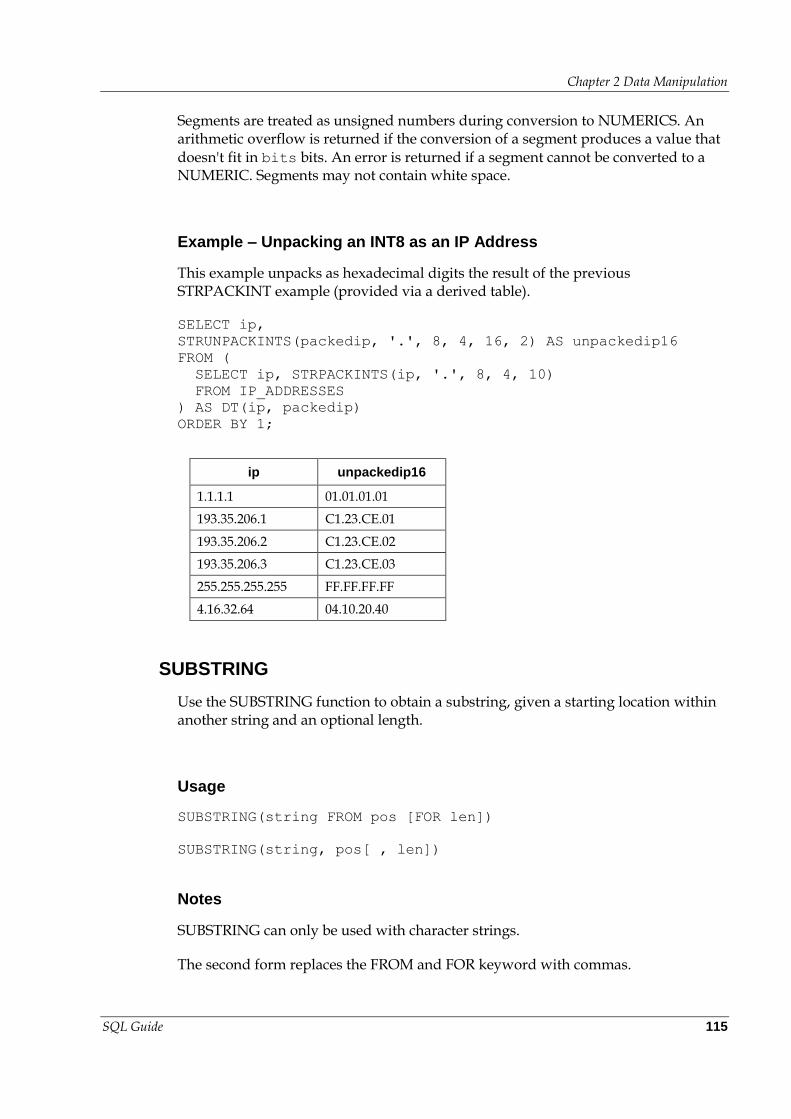
Chapter 2 Data Manipulation
SQL Guide 115
Segments are treated as unsigned numbers during conversion to NUMERICS. An arithmetic overflow is returned if the conversion of a segment produces a value that doesn't fit in bits bits. An error is returned if a segment cannot be converted to a NUMERIC. Segments may not contain white space.
Example – Unpacking an INT8 as an IP Address
This example unpacks as hexadecimal digits the result of the previous STRPACKINT example (provided via a derived table).
SELECT ip,
STRUNPACKINTS(packedip, '.', 8, 4, 16, 2) AS unpackedip16
FROM (
SELECT ip, STRPACKINTS(ip, '.', 8, 4, 10)
FROM IP_ADDRESSES
) AS DT(ip, packedip)
ORDER BY 1;
ip unpackedip16
1.1.1.1 01.01.01.01
193.35.206.1 C1.23.CE.01
193.35.206.2 C1.23.CE.02
193.35.206.3 C1.23.CE.03
255.255.255.255 FF.FF.FF.FF
4.16.32.64 04.10.20.40
SUBSTRING
Use the SUBSTRING function to obtain a substring, given a starting location within another string and an optional length.
Usage
SUBSTRING(string FROM pos [FOR len])
SUBSTRING(string, pos[ , len])
Notes
SUBSTRING can only be used with character strings.
The second form replaces the FROM and FOR keyword with commas.
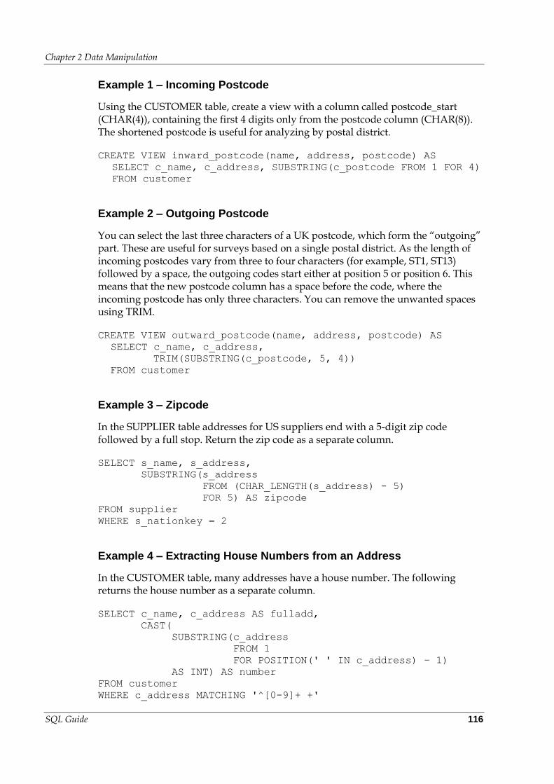
Chapter 2 Data Manipulation
SQL Guide 116
Example 1 – Incoming Postcode
Using the CUSTOMER table, create a view with a column called postcode_start (CHAR(4)), containing the first 4 digits only from the postcode column (CHAR(8)). The shortened postcode is useful for analyzing by postal district.
CREATE VIEW inward_postcode(name, address, postcode) AS
SELECT c_name, c_address, SUBSTRING(c_postcode FROM 1 FOR 4)
FROM customer
Example 2 – Outgoing Postcode
You can select the last three characters of a UK postcode, which form the “outgoing” part. These are useful for surveys based on a single postal district. As the length of incoming postcodes vary from three to four characters (for example, ST1, ST13) followed by a space, the outgoing codes start either at position 5 or position 6. This means that the new postcode column has a space before the code, where the incoming postcode has only three characters. You can remove the unwanted spaces using TRIM.
CREATE VIEW outward_postcode(name, address, postcode) AS
SELECT c_name, c_address,
TRIM(SUBSTRING(c_postcode, 5, 4))
FROM customer
Example 3 – Zipcode
In the SUPPLIER table addresses for US suppliers end with a 5-digit zip code followed by a full stop. Return the zip code as a separate column.
SELECT s_name, s_address,
SUBSTRING(s_address
FROM (CHAR_LENGTH(s_address) - 5)
FOR 5) AS zipcode
FROM supplier
WHERE s_nationkey = 2
Example 4 – Extracting House Numbers from an Address
In the CUSTOMER table, many addresses have a house number. The following returns the house number as a separate column.
SELECT c_name, c_address AS fulladd,
CAST(
SUBSTRING(c_address
FROM 1
FOR POSITION(' ' IN c_address) – 1)
AS INT) AS number
FROM customer
WHERE c_address MATCHING '^[0-9]+ +'
Chapter 2 Data Manipulation
SQL Guide 117
ORDER BY 3
SYSDATE
SYSDATE is a synonym for CURRENT_TIMESTAMP. See CURRENT_TIMESTAMP.
TABLE_ID
The TABLE_ID function is useful for querying system tables.
Usage
TABLE_ID(table)
Notes
The argument is an unquoted string that specifies the table name; it can include the schema name and separator.
Example
Previously a query of the following form had to be used when a reference to the ID of a table was required:
SELECT * FROM ipe_allcol_img
WHERE table_id = (
SELECT id FROM ipe_alltable WHERE name = 'IPE_COMMAND')
This query can now be written as:
SELECT * FROM ipe_allcol_img
WHERE table_id = TABLE_ID(IPE_COMMAND)
TAN
TAN calculates the tangent for the specified argument.
Usage
TAN(argument)
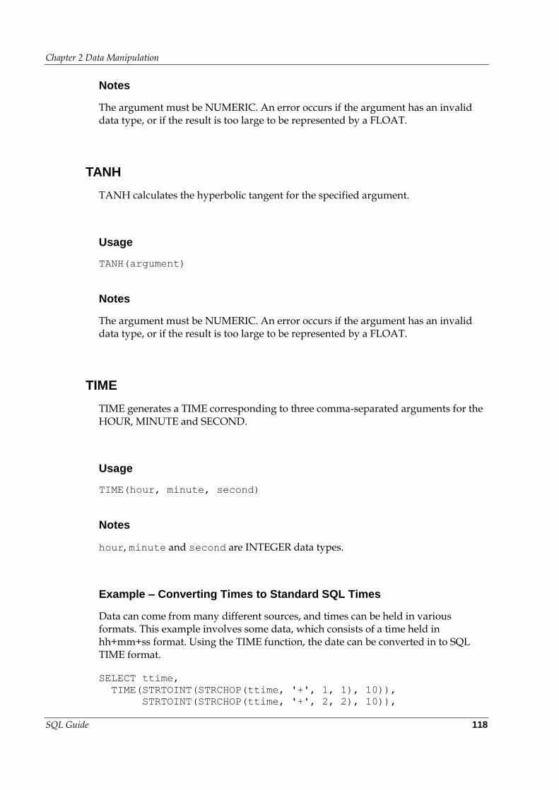
Chapter 2 Data Manipulation
SQL Guide 118
Notes
The argument must be NUMERIC. An error occurs if the argument has an invalid data type, or if the result is too large to be represented by a FLOAT.
TANH
TANH calculates the hyperbolic tangent for the specified argument.
Usage
TANH(argument)
Notes
The argument must be NUMERIC. An error occurs if the argument has an invalid data type, or if the result is too large to be represented by a FLOAT.
TIME
TIME generates a TIME corresponding to three comma-separated arguments for the HOUR, MINUTE and SECOND.
Usage
TIME(hour, minute, second)
Notes
hour, minute and second are INTEGER data types.
Example – Converting Times to Standard SQL Times
Data can come from many different sources, and times can be held in various formats. This example involves some data, which consists of a time held in hh+mm+ss format. Using the TIME function, the date can be converted in to SQL TIME format.
SELECT ttime,
TIME(STRTOINT(STRCHOP(ttime, '+', 1, 1), 10)),
STRTOINT(STRCHOP(ttime, '+', 2, 2), 10)),
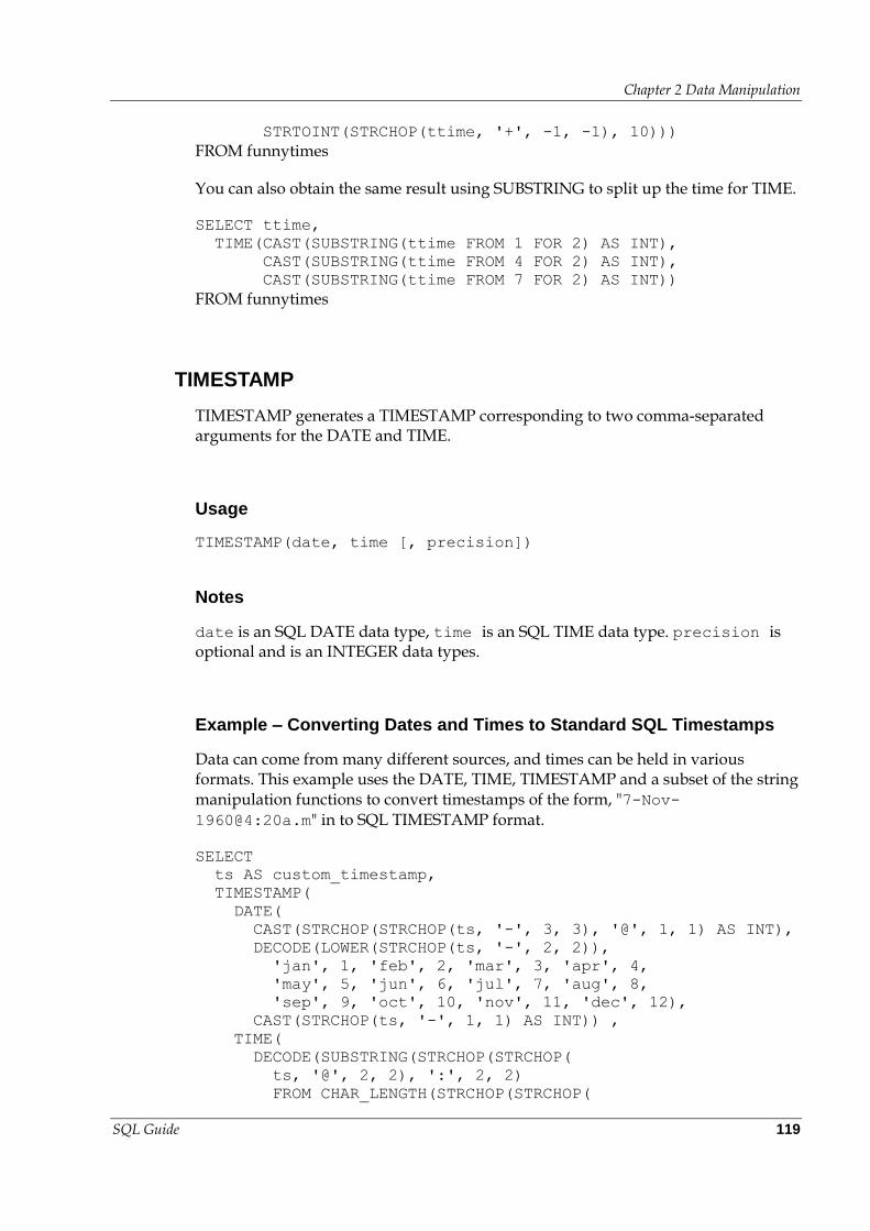
Chapter 2 Data Manipulation
SQL Guide 119
STRTOINT(STRCHOP(ttime, '+', -1, -1), 10)))
FROM funnytimes
You can also obtain the same result using SUBSTRING to split up the time for TIME.
SELECT ttime,
TIME(CAST(SUBSTRING(ttime FROM 1 FOR 2) AS INT),
CAST(SUBSTRING(ttime FROM 4 FOR 2) AS INT),
CAST(SUBSTRING(ttime FROM 7 FOR 2) AS INT))
FROM funnytimes
TIMESTAMP
TIMESTAMP generates a TIMESTAMP corresponding to two comma-separated arguments for the DATE and TIME.
Usage
TIMESTAMP(date, time [, precision])
Notes
date is an SQL DATE data type, time is an SQL TIME data type. precision is optional and is an INTEGER data types.
Example – Converting Dates and Times to Standard SQL Timestamps
Data can come from many different sources, and times can be held in various formats. This example uses the DATE, TIME, TIMESTAMP and a subset of the string manipulation functions to convert timestamps of the form, "7-Nov-
1960@4:20a.m" in to SQL TIMESTAMP format.
SELECT
ts AS custom_timestamp,
TIMESTAMP(
DATE(
CAST(STRCHOP(STRCHOP(ts, '-', 3, 3), '@', 1, 1) AS INT),
DECODE(LOWER(STRCHOP(ts, '-', 2, 2)),
'jan', 1, 'feb', 2, 'mar', 3, 'apr', 4,
'may', 5, 'jun', 6, 'jul', 7, 'aug', 8,
'sep', 9, 'oct', 10, 'nov', 11, 'dec', 12),
CAST(STRCHOP(ts, '-', 1, 1) AS INT)) ,
TIME(
DECODE(SUBSTRING(STRCHOP(STRCHOP(
ts, '@', 2, 2), ':', 2, 2)
FROM CHAR_LENGTH(STRCHOP(STRCHOP(
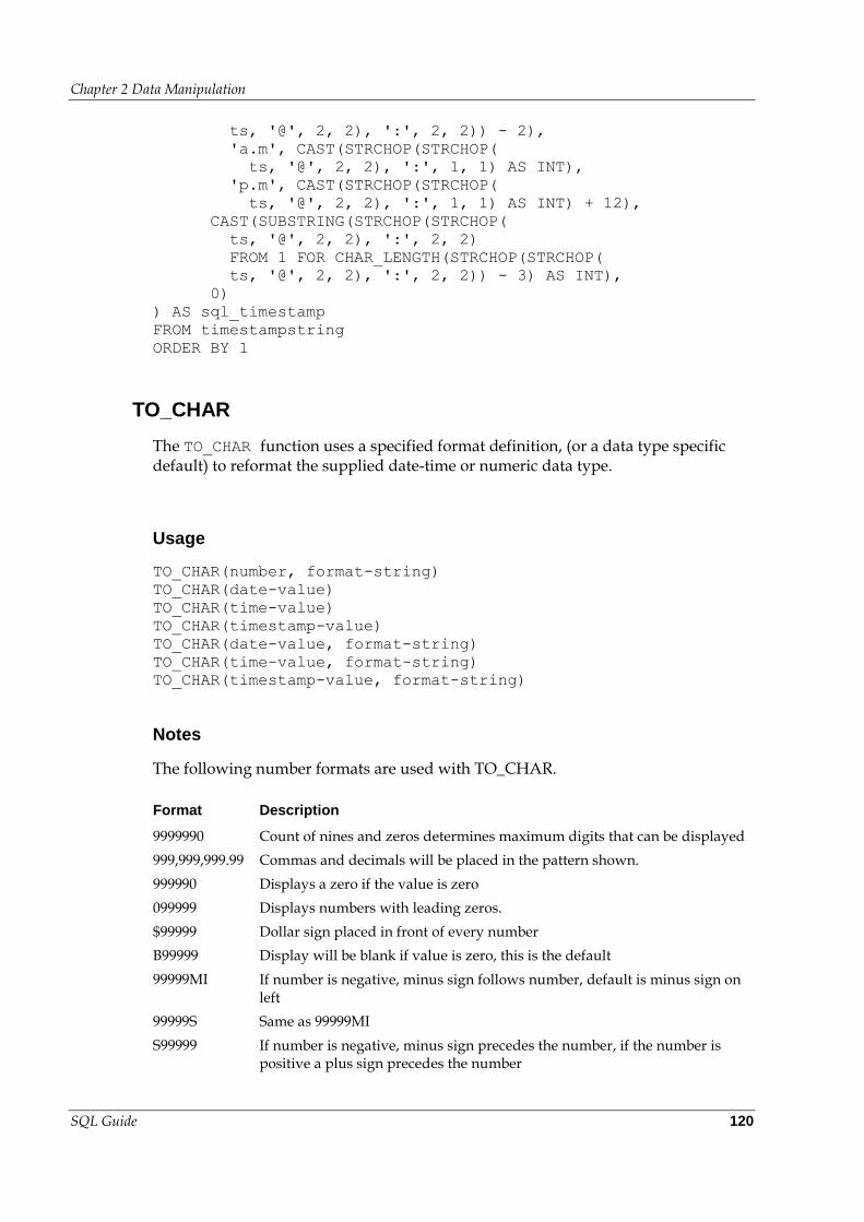
Chapter 2 Data Manipulation
SQL Guide 120
ts, '@', 2, 2), ':', 2, 2)) - 2),
'a.m', CAST(STRCHOP(STRCHOP(
ts, '@', 2, 2), ':', 1, 1) AS INT),
'p.m', CAST(STRCHOP(STRCHOP(
ts, '@', 2, 2), ':', 1, 1) AS INT) + 12),
CAST(SUBSTRING(STRCHOP(STRCHOP(
ts, '@', 2, 2), ':', 2, 2)
FROM 1 FOR CHAR_LENGTH(STRCHOP(STRCHOP(
ts, '@', 2, 2), ':', 2, 2)) - 3) AS INT),
0)
) AS sql_timestamp
FROM timestampstring
ORDER BY 1
TO_CHAR
The TO_CHAR function uses a specified format definition, (or a data type specific default) to reformat the supplied date-time or numeric data type.
Usage
TO_CHAR(number, format-string)
TO_CHAR(date-value)
TO_CHAR(time-value)
TO_CHAR(timestamp-value)
TO_CHAR(date-value, format-string)
TO_CHAR(time-value, format-string)
TO_CHAR(timestamp-value, format-string)
Notes
The following number formats are used with TO_CHAR.
Format Description
9999990 Count of nines and zeros determines maximum digits that can be displayed
999,999,999.99 Commas and decimals will be placed in the pattern shown.
999990 Displays a zero if the value is zero
099999 Displays numbers with leading zeros.
$99999 Dollar sign placed in front of every number
B99999 Display will be blank if value is zero, this is the default
99999MI If number is negative, minus sign follows number, default is minus sign on left
99999S Same as 99999MI
S99999 If number is negative, minus sign precedes the number, if the number is positive a plus sign precedes the number
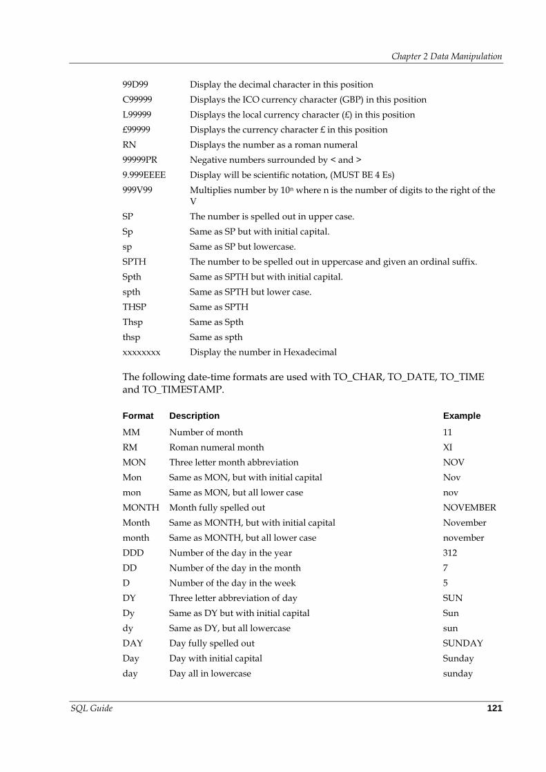
Chapter 2 Data Manipulation
SQL Guide 121
99D99 Display the decimal character in this position
C99999 Displays the ICO currency character (GBP) in this position
L99999 Displays the local currency character (£) in this position
£99999 Displays the currency character £ in this position
RN Displays the number as a roman numeral
99999PR Negative numbers surrounded by < and >
9.999EEEE Display will be scientific notation, (MUST BE 4 Es)
999V99 Multiplies number by 10n where n is the number of digits to the right of the V
SP The number is spelled out in upper case.
Sp Same as SP but with initial capital.
sp Same as SP but lowercase.
SPTH The number to be spelled out in uppercase and given an ordinal suffix.
Spth Same as SPTH but with initial capital.
spth Same as SPTH but lower case.
THSP Same as SPTH
Thsp Same as Spth
thsp Same as spth
xxxxxxxx Display the number in Hexadecimal
The following date-time formats are used with TO_CHAR, TO_DATE, TO_TIME and TO_TIMESTAMP.
Format Description Example
MM Number of month 11
RM Roman numeral month XI
MON Three letter month abbreviation NOV
Mon Same as MON, but with initial capital Nov
mon Same as MON, but all lower case nov
MONTH Month fully spelled out NOVEMBER
Month Same as MONTH, but with initial capital November
month Same as MONTH, but all lower case november
DDD Number of the day in the year 312
DD Number of the day in the month 7
D Number of the day in the week 5
DY Three letter abbreviation of day SUN
Dy Same as DY but with initial capital Sun
dy Same as DY, but all lowercase sun
DAY Day fully spelled out SUNDAY
Day Day with initial capital Sunday
day Day all in lowercase sunday
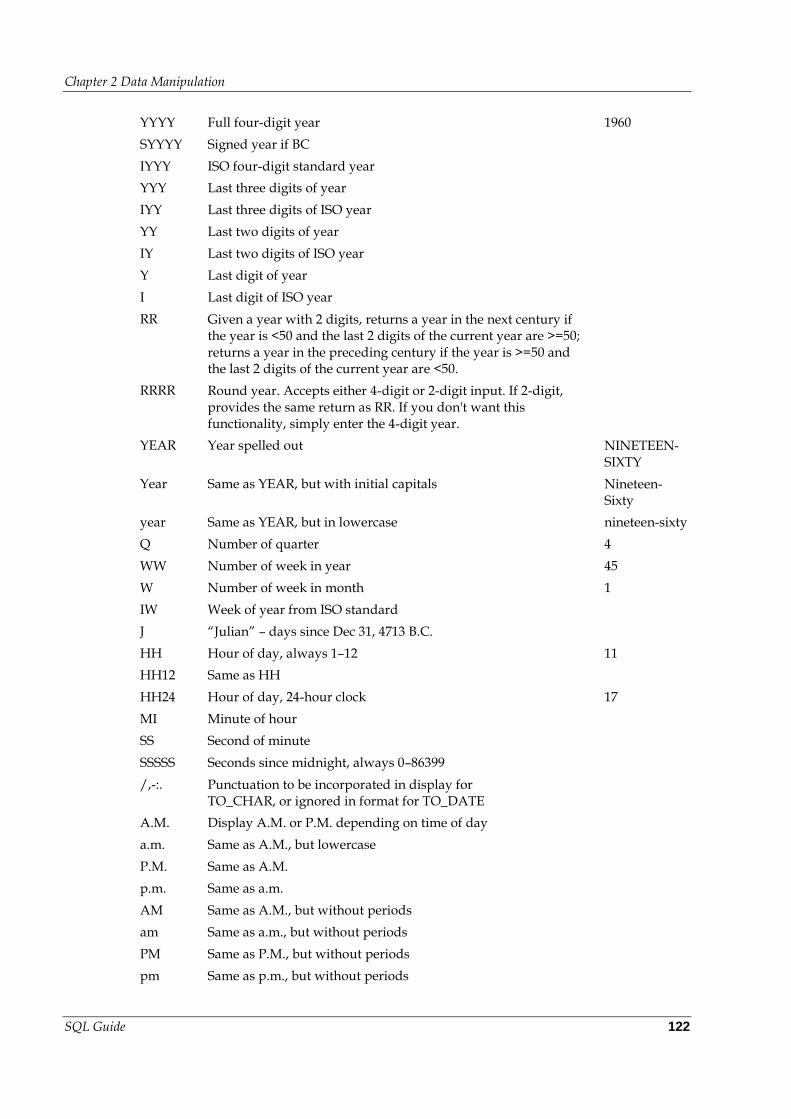
Chapter 2 Data Manipulation
SQL Guide 122
YYYY Full four-digit year 1960
SYYYY Signed year if BC
IYYY ISO four-digit standard year
YYY Last three digits of year
IYY Last three digits of ISO year
YY Last two digits of year
IY Last two digits of ISO year
Y Last digit of year
I Last digit of ISO year
RR Given a year with 2 digits, returns a year in the next century if the year is <50 and the last 2 digits of the current year are >=50; returns a year in the preceding century if the year is >=50 and the last 2 digits of the current year are <50.
RRRR Round year. Accepts either 4-digit or 2-digit input. If 2-digit, provides the same return as RR. If you don't want this functionality, simply enter the 4-digit year.
YEAR Year spelled out NINETEEN-SIXTY
Year Same as YEAR, but with initial capitals Nineteen-Sixty
year Same as YEAR, but in lowercase nineteen-sixty
Q Number of quarter 4
WW Number of week in year 45
W Number of week in month 1
IW Week of year from ISO standard
J “Julian” – days since Dec 31, 4713 B.C.
HH Hour of day, always 1–12 11
HH12 Same as HH
HH24 Hour of day, 24-hour clock 17
MI Minute of hour
SS Second of minute
SSSSS Seconds since midnight, always 0–86399
/,-:. Punctuation to be incorporated in display for TO_CHAR, or ignored in format for TO_DATE
A.M. Display A.M. or P.M. depending on time of day
a.m. Same as A.M., but lowercase
P.M. Same as A.M.
p.m. Same as a.m.
AM Same as A.M., but without periods
am Same as a.m., but without periods
PM Same as P.M., but without periods
pm Same as p.m., but without periods
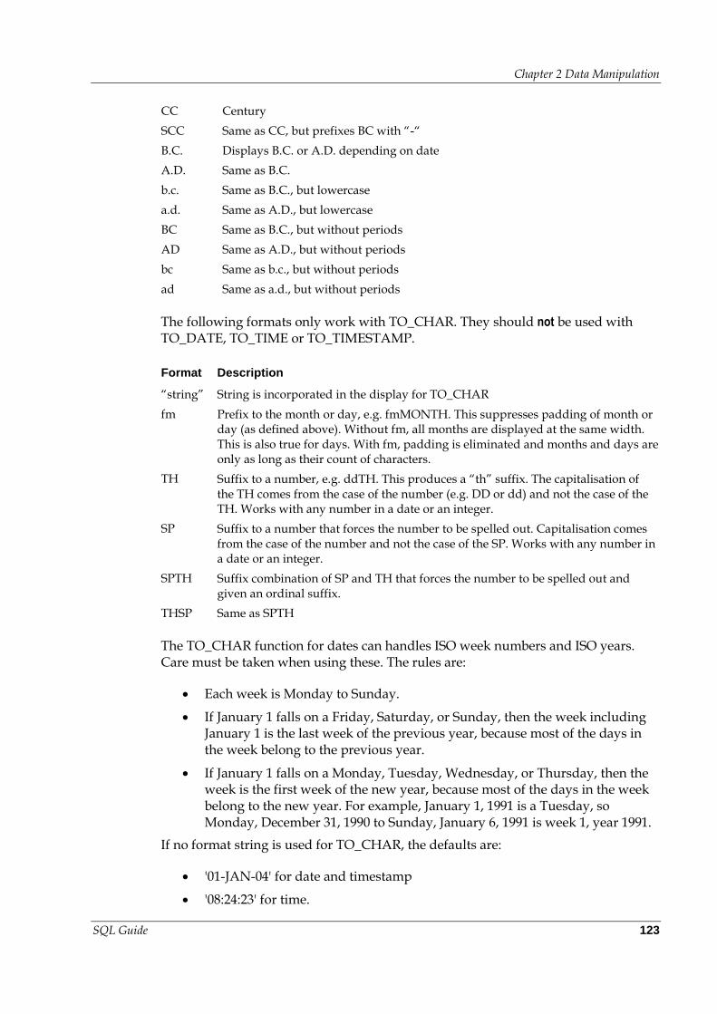
Chapter 2 Data Manipulation
SQL Guide 123
CC Century
SCC Same as CC, but prefixes BC with “-“
B.C. Displays B.C. or A.D. depending on date
A.D. Same as B.C.
b.c. Same as B.C., but lowercase
a.d. Same as A.D., but lowercase
BC Same as B.C., but without periods
AD Same as A.D., but without periods
bc Same as b.c., but without periods
ad Same as a.d., but without periods
The following formats only work with TO_CHAR. They should not be used with TO_DATE, TO_TIME or TO_TIMESTAMP.
Format Description
“string” String is incorporated in the display for TO_CHAR
fm Prefix to the month or day, e.g. fmMONTH. This suppresses padding of month or day (as defined above). Without fm, all months are displayed at the same width. This is also true for days. With fm, padding is eliminated and months and days are only as long as their count of characters.
TH Suffix to a number, e.g. ddTH. This produces a “th” suffix. The capitalisation of the TH comes from the case of the number (e.g. DD or dd) and not the case of the TH. Works with any number in a date or an integer.
SP Suffix to a number that forces the number to be spelled out. Capitalisation comes from the case of the number and not the case of the SP. Works with any number in a date or an integer.
SPTH Suffix combination of SP and TH that forces the number to be spelled out and given an ordinal suffix.
THSP Same as SPTH
The TO_CHAR function for dates can handles ISO week numbers and ISO years. Care must be taken when using these. The rules are:
Each week is Monday to Sunday.
If January 1 falls on a Friday, Saturday, or Sunday, then the week including January 1 is the last week of the previous year, because most of the days in the week belong to the previous year.
If January 1 falls on a Monday, Tuesday, Wednesday, or Thursday, then the week is the first week of the new year, because most of the days in the week belong to the new year. For example, January 1, 1991 is a Tuesday, so Monday, December 31, 1990 to Sunday, January 6, 1991 is week 1, year 1991.
If no format string is used for TO_CHAR, the defaults are:
'01-JAN-04' for date and timestamp
'08:24:23' for time.
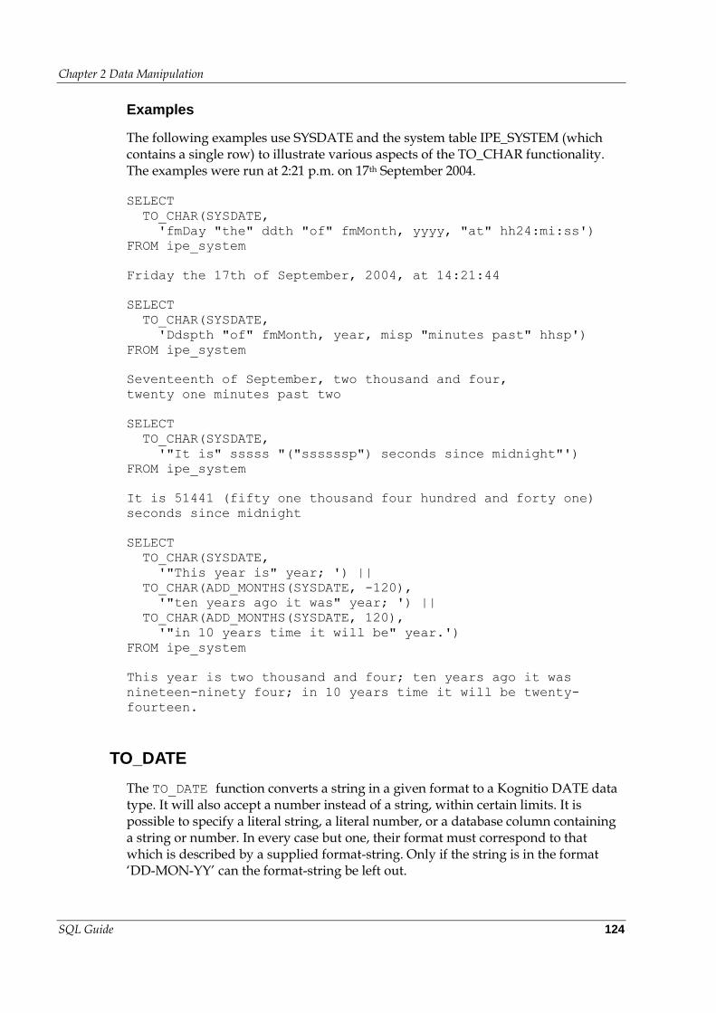
Chapter 2 Data Manipulation
SQL Guide 124
Examples
The following examples use SYSDATE and the system table IPE_SYSTEM (which contains a single row) to illustrate various aspects of the TO_CHAR functionality. The examples were run at 2:21 p.m. on 17th September 2004.
SELECT
TO_CHAR(SYSDATE,
'fmDay "the" ddth "of" fmMonth, yyyy, "at" hh24:mi:ss')
FROM ipe_system
Friday the 17th of September, 2004, at 14:21:44
SELECT
TO_CHAR(SYSDATE,
'Ddspth "of" fmMonth, year, misp "minutes past" hhsp')
FROM ipe_system
Seventeenth of September, two thousand and four,
twenty one minutes past two
SELECT
TO_CHAR(SYSDATE,
'"It is" sssss "("ssssssp") seconds since midnight"')
FROM ipe_system
It is 51441 (fifty one thousand four hundred and forty one)
seconds since midnight
SELECT
TO_CHAR(SYSDATE,
'"This year is" year; ') ||
TO_CHAR(ADD_MONTHS(SYSDATE, -120),
'"ten years ago it was" year; ') ||
TO_CHAR(ADD_MONTHS(SYSDATE, 120),
'"in 10 years time it will be" year.')
FROM ipe_system
This year is two thousand and four; ten years ago it was
nineteen-ninety four; in 10 years time it will be twenty-
fourteen.
TO_DATE
The TO_DATE function converts a string in a given format to a Kognitio DATE data type. It will also accept a number instead of a string, within certain limits. It is possible to specify a literal string, a literal number, or a database column containing a string or number. In every case but one, their format must correspond to that which is described by a supplied format-string. Only if the string is in the format ‘DD-MON-YY’ can the format-string be left out.
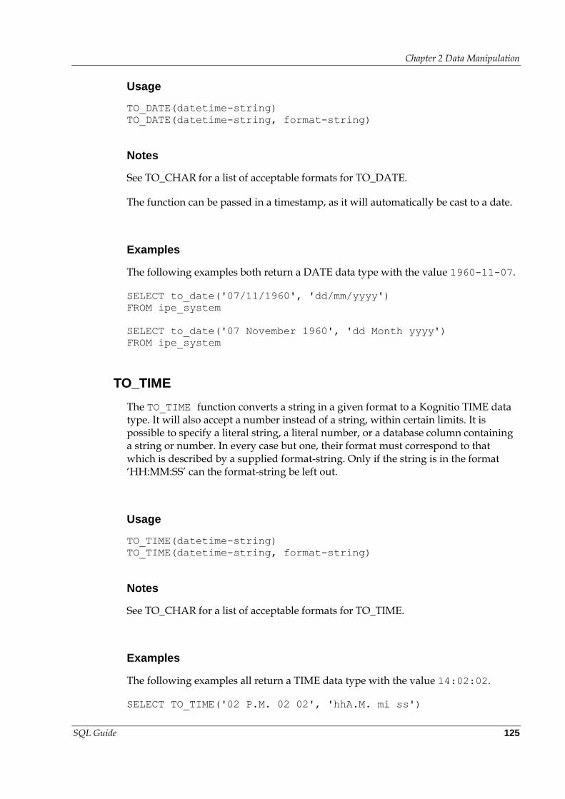
Chapter 2 Data Manipulation
SQL Guide 125
Usage
TO_DATE(datetime-string)
TO_DATE(datetime-string, format-string)
Notes
See TO_CHAR for a list of acceptable formats for TO_DATE.
The function can be passed in a timestamp, as it will automatically be cast to a date.
Examples
The following examples both return a DATE data type with the value 1960-11-07.
SELECT to_date('07/11/1960', 'dd/mm/yyyy')
FROM ipe_system
SELECT to_date('07 November 1960', 'dd Month yyyy')
FROM ipe_system
TO_TIME
The TO_TIME function converts a string in a given format to a Kognitio TIME data type. It will also accept a number instead of a string, within certain limits. It is possible to specify a literal string, a literal number, or a database column containing a string or number. In every case but one, their format must correspond to that which is described by a supplied format-string. Only if the string is in the format ‘HH:MM:SS’ can the format-string be left out.
Usage
TO_TIME(datetime-string)
TO_TIME(datetime-string, format-string)
Notes
See TO_CHAR for a list of acceptable formats for TO_TIME.
Examples
The following examples all return a TIME data type with the value 14:02:02.
SELECT TO_TIME('02 P.M. 02 02', 'hhA.M. mi ss')
Chapter 2 Data Manipulation
SQL Guide 126
FROM ipe_system
SELECT TO_TIME('14:02:02')
FROM ipe_system;
SELECT TO_TIME('50522', 'SSSSS')
FROM ipe_system;
TO_TIMESTAMP
The TO_TIMESTAMP function converts a string in a given format to a Kognitio TIMESTAMP data type. It will also accept a number instead of a string, within certain limits. It is possible to specify a literal string, a literal number, or a database column containing a string or number. In every case but one, their format must correspond to that which is described by a supplied format-string. Only if the string is in the format ‘DD-MON-YY HH:MM:SS’ can the format-string be left out.
Usage
TO_TIMESTAMP(datetime-string)
TO_TIMESTAMP(datetime-string, format-string)
Notes
See TO_CHAR for a list of acceptable formats for TO_TIMESTAMP.
Examples
The following examples both return a TIMESTAMP data type with the value 1960-11-07 14:02:02.
SELECT TO_TIMESTAMP('14-02-02-07-11-1960',
'hh-mi-ss-dd-mm-yyyy')
FROM ipe_system;
SELECT TO_TIMESTAMP('07/11/[email protected]. 02:02',
'dd/mm/[email protected]. mi:ss')
FROM ipe_system;
TRIM
Use the TRIM function to remove one or more occurrence of any individual character (typically a space)—LEADING, TRAILING or BOTH, from a string.
Chapter 2 Data Manipulation
SQL Guide 127
Usage
TRIM([BOTH | LEADING | TRAILING] [character] FROM string)
Notes
You can only use the TRIM function to trim character strings.
If BOTH, LEADING and TRAILING are not present, BOTH is assumed. If the character is not specified a space is assumed.
If BOTH, LEADING, TRAILING and character-expression are not present then the key word FROM must be omitted as well.
Example 1 – Trim any spaces that surround a name
The following will remove any leading and trailing spaces from the customer name.
SELECT TRIM(c_name)
FROM customer
Note: This is equivalent to, but much more convenient than:
SELECT TRIM(BOTH ' ' FROM c_name)
FROM customer.
If the spaces were actually tabs then you could use the following:
SELECT TRIM(BOTH CHR(9) FROM c_name)
FROM customer
Example 2 – TRIM TRAILING
The postcode column in the CUSTOMER table is a CHAR(9), but as postcodes contain either seven or eight characters there are trailing spaces. If you want to concatenate the postcode with a string literal that adds a comma and then the nation, you need to remove the trailing spaces.
SELECT customer.c_name customer,
customer.c_address || ', ' ||
TRIM(TRAILING ' ' FROM customer.c_postcode) || ', ' ||
nation.n_name long_address
FROM customer, nation
WHERE customer.c_nationkey = nation.n_nationkey
ORDER BY 1
Note: As there aren't any leading spaces on the postcode column, the above query could actually be written as:
Chapter 2 Data Manipulation
SQL Guide 128
SELECT customer.c_name customer,
customer.c_address || ', ' ||
TRIM(customer.c_postcode) || ', ' ||
nation.n_name long_address
FROM customer, nation
WHERE customer.c_nationkey = nation.n_nationkey
ORDER BY 1
Example 3 – Nested TRIMs
In the SUPPLIER table addresses end with a full stop. If you want to add the nation name to the address with a comma separator, you need to TRIM the full stop, and also any trailing spaces. (This requires nested TRIM functions.)
SELECT supplier.s_suppkey, supplier.s_name,
TRIM(TRAILING '.' FROM
TRIM(TRAILING ' ' FROM supplier.s_address)) ||
', ' || nation.n_name AS longaddress
FROM supplier_a, nation
WHERE supplier_a.s_nationkey = nation.n_nationkey
ORDER BY 1
UCHR
UCHR returns the character representation of a Unicode codepoint.
Usage
UCHR(codepoint)
Example
SELECT UCHR(H'20AC')
Returns the Euro symbol (€).
UNICODE
UNICODE returns the codepoint representation of a Unicode character.
Usage
UNICODE(char)
Chapter 2 Data Manipulation
SQL Guide 129
Example
SELECT UNICODE('€')
Returns 8364, the decimal representation of the Euro symbol (€).
UPPER
Use the UPPER function to convert a given string to upper case.
Usage
UPPER(string)
Notes
UPPER can only be used to convert character strings.
Example
This example obtains details of all the Smalltown suppliers without an ST1 postcode. Here, LOWER is used before s_address in the first WHERE condition, so that LIKE ‘%smalltown%’ can match addresses entered as ‘smalltown’, ‘Smalltown’ or ‘SMALLTOWN’. UPPER is used with the second WHERE condition, to ensure the LIKE condition (‘ST1 %') matches all occurrences of ST1, regardless of case.
SELECT *
FROM supplier
WHERE LOWER(s_address) LIKE '%smalltown%' AND
UPPER(s_address) NOT LIKE 'ST1 %'
ORDER BY s_suppkey
USER
This returns the user name for the current session.
Example
The following obtains the current user name and their id.
SELECT USER, CURRENT_USER_ID
Chapter 2 Data Manipulation
SQL Guide 130
USER_ID
The USER_ID function is useful for querying system tables.
Usage
USER_ID(user)
Notes
The argument is an unquoted string that specifies the user name.
Example
The following query can be used to determine the schema currently associated with a user:
SELECT name, id FROM ipe_schema
WHERE user_id = USER_ID(MJB)
VAL_AT_POSN
The VAL_AT_POSN function returns the value from a list of expressions at the specified position. If the position does not exist then the function result is NULL. This function is added as the converse of the POSN_IN_LIST function. It is probably far less useful as typically the required value will be available, possibly having been supplied directly to the POSN_IN_LIST function.
Usage
VAL_AT_POSN(position, expression-list)
Example
The following example uses VAL_AT_POSN to sum the second and third highest quarters from the quarterly summary view.
SELECT region, office, octtotal, novtotal, dectotal,
GREATEST(octtotal, novtotal, dectotal) largest,
VAL_AT_POSN(
DECODE(
POSN_IN_LIST(
GREATEST(octtotal, novtotal, dectotal),
octtotal, novtotal, dectotal),
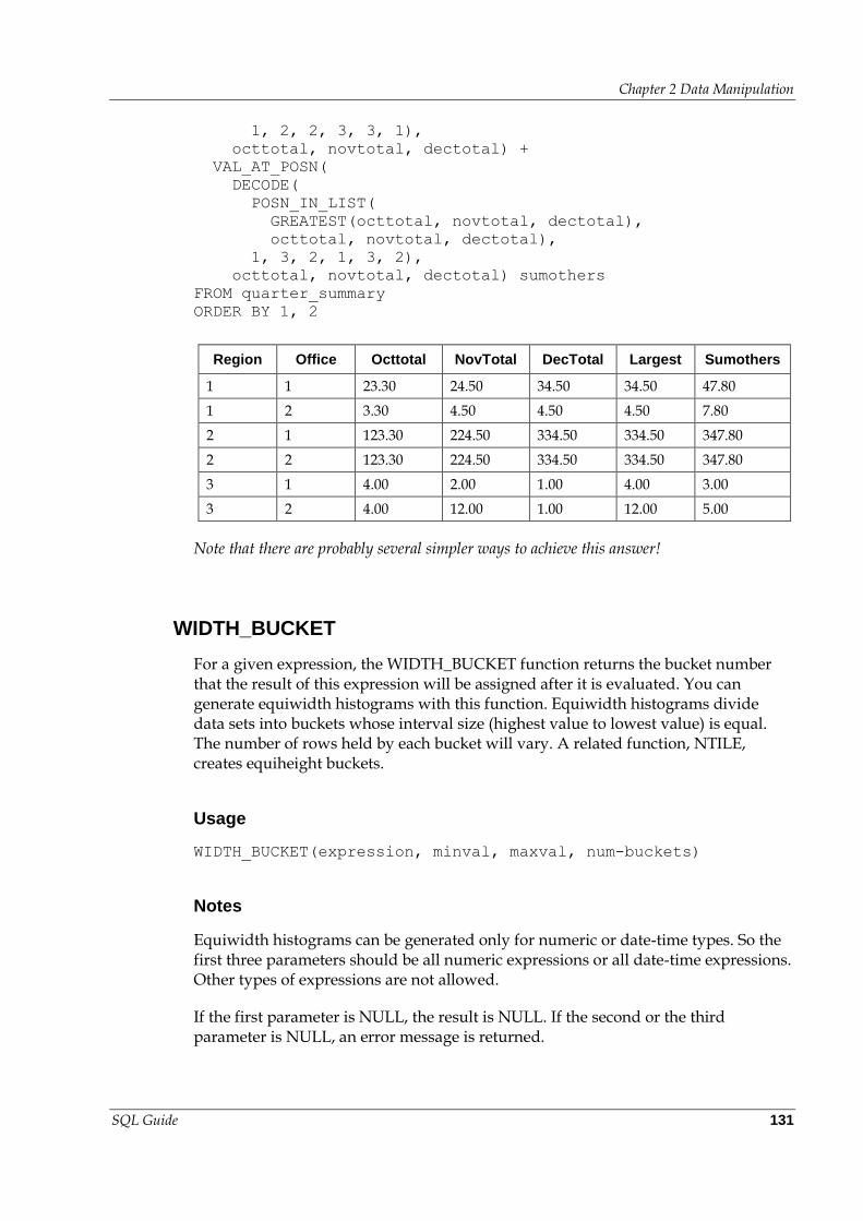
Chapter 2 Data Manipulation
SQL Guide 131
1, 2, 2, 3, 3, 1),
octtotal, novtotal, dectotal) +
VAL_AT_POSN(
DECODE(
POSN_IN_LIST(
GREATEST(octtotal, novtotal, dectotal),
octtotal, novtotal, dectotal),
1, 3, 2, 1, 3, 2),
octtotal, novtotal, dectotal) sumothers
FROM quarter_summary
ORDER BY 1, 2
Region Office Octtotal NovTotal DecTotal Largest Sumothers
1 1 23.30 24.50 34.50 34.50 47.80
1 2 3.30 4.50 4.50 4.50 7.80
2 1 123.30 224.50 334.50 334.50 347.80
2 2 123.30 224.50 334.50 334.50 347.80
3 1 4.00 2.00 1.00 4.00 3.00
3 2 4.00 12.00 1.00 12.00 5.00
Note that there are probably several simpler ways to achieve this answer!
WIDTH_BUCKET
For a given expression, the WIDTH_BUCKET function returns the bucket number that the result of this expression will be assigned after it is evaluated. You can generate equiwidth histograms with this function. Equiwidth histograms divide data sets into buckets whose interval size (highest value to lowest value) is equal. The number of rows held by each bucket will vary. A related function, NTILE, creates equiheight buckets.
Usage
WIDTH_BUCKET(expression, minval, maxval, num-buckets)
Notes
Equiwidth histograms can be generated only for numeric or date-time types. So the first three parameters should be all numeric expressions or all date-time expressions. Other types of expressions are not allowed.
If the first parameter is NULL, the result is NULL. If the second or the third parameter is NULL, an error message is returned.
Chapter 2 Data Manipulation
SQL Guide 132
The last parameter (number of buckets) should be a numeric expression that evaluates to a positive integer value; 0, NULL, or a negative value will result in an error.
Buckets are numbered from 0 to (n+1). Bucket 0 holds the count of values less than the minimum. Bucket(n+1) holds the count of values greater than or equal to the maximum specified value.
Each bucket is a closed-open interval of the real number line, for example, a bucket that is assigned to scores between 5000.0000 and 9999.9999..., is denoted [5000, 10000) to indicate that 5,000 is included in the interval and 10,000 is excluded.
Example
The following example shows the bucket number for the total price of all orders placed in 1998.
SELECT
o_custkey,
o_totalprice,
WIDTH_BUCKET(o_totalprice, 0, 10000, 5) AS bucket
FROM
ordertab
WHERE
o_orderdate BETWEEN DATE '1998-01-01' AND DATE '1998-12-31'
WX_CREATE_TNO
The WX_CREATE_TNO function returns the transaction number that created the associated row.
Usage
WX_CREATE_TNO()
Notes
Although no parameters are supplied to the function the parentheses are required.
The function is primarily for use by the Kognitio archiving mechanism.
To make full use of the function the FULL_HISTORY snapshot may be required.
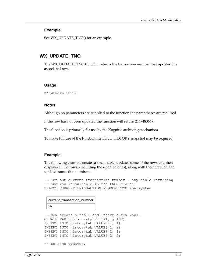
Chapter 2 Data Manipulation
SQL Guide 133
Example
See WX_UPDATE_TNO() for an example.
WX_UPDATE_TNO
The WX_UPDATE_TNO function returns the transaction number that updated the associated row.
Usage
WX_UPDATE_TNO()
Notes
Although no parameters are supplied to the function the parentheses are required.
If the row has not been updated the function will return 2147483647.
The function is primarily for use by the Kognitio archiving mechanism.
To make full use of the function the FULL_HISTORY snapshot may be required.
Example
The following example creates a small table, updates some of the rows and then displays all the rows, (Including the updated ones), along with their creation and update transaction numbers.
-- Get out current transaction number - any table returning
-- one row is suitable in the FROM clause.
SELECT CURRENT_TRANSACTION_NUMBER FROM ipe_system
current_transaction_number
565
-- Now create a table and insert a few rows.
CREATE TABLE historytab(i INT, j INT)
INSERT INTO historytab VALUES(1, 1)
INSERT INTO historytab VALUES(1, 2)
INSERT INTO historytab VALUES(2, 1)
INSERT INTO historytab VALUES(2, 2)
-- Do some updates.
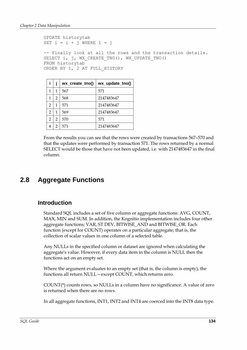
Chapter 2 Data Manipulation
SQL Guide 134
UPDATE historytab
SET i = i + j WHERE i = j
-- Finally look at all the rows and the transaction details.
SELECT i, j, WX_CREATE_TNO(), WX_UPDATE_TNO()
FROM historytab
ORDER BY 1, 2 AT FULL_HISTORY
i j wx_create_tno() wx_update_tno()
1 1 567 571
1 2 568 2147483647
2 1 571 2147483647
2 1 569 2147483647
2 2 570 571
4 2 571 2147483647
From the results you can see that the rows were created by transactions 567–570 and that the updates were performed by transaction 571. The rows returned by a normal SELECT would be those that have not been updated, i.e. with 2147483647 in the final column.
2.8 Aggregate Functions
Introduction
Standard SQL includes a set of five column or aggregate functions: AVG, COUNT, MAX, MIN and SUM. In addition, the Kognitio implementation includes four other aggregate functions; VAR, ST DEV, BITWISE_AND and BITWISE_OR. Each function (except for COUNT) operates on a particular aggregate; that is, the collection of scalar values in one column of a selected table.
Any NULLs in the specified column or dataset are ignored when calculating the aggregate's value. However, if every data item in the column is NULL then the functions act on an empty set.
Where the argument evaluates to an empty set (that is, the column is empty), the functions all return NULL—except COUNT, which returns zero.
COUNT(*) counts rows, so NULLs in a column have no significance. A value of zero is returned when there are no rows.
In all aggregate functions, INT1, INT2 and INT4 are coerced into the INT8 data type.
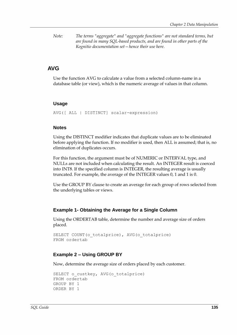
Chapter 2 Data Manipulation
SQL Guide 135
Note: The terms "aggregate" and "aggregate functions" are not standard terms, but are found in many SQL-based products, and are found in other parts of the Kognitio documentation set—hence their use here.
AVG
Use the function AVG to calculate a value from a selected column-name in a database table (or view), which is the numeric average of values in that column.
Usage
AVG([ ALL | DISTINCT] scalar-expression)
Notes
Using the DISTINCT modifier indicates that duplicate values are to be eliminated before applying the function. If no modifier is used, then ALL is assumed; that is, no elimination of duplicates occurs.
For this function, the argument must be of NUMERIC or INTERVAL type, and NULLs are not included when calculating the result. An INTEGER result is coerced into INT8. If the specified column is INTEGER, the resulting average is usually truncated. For example, the average of the INTEGER values 0, 1 and 1 is 0.
Use the GROUP BY clause to create an average for each group of rows selected from the underlying tables or views.
Example 1- Obtaining the Average for a Single Column
Using the ORDERTAB table, determine the number and average size of orders placed.
SELECT COUNT(o_totalprice), AVG(o_totalprice)
FROM ordertab
Example 2 – Using GROUP BY
Now, determine the average size of orders placed by each customer.
SELECT o_custkey, AVG(o_totalprice)
FROM ordertab
GROUP BY 1
ORDER BY 1
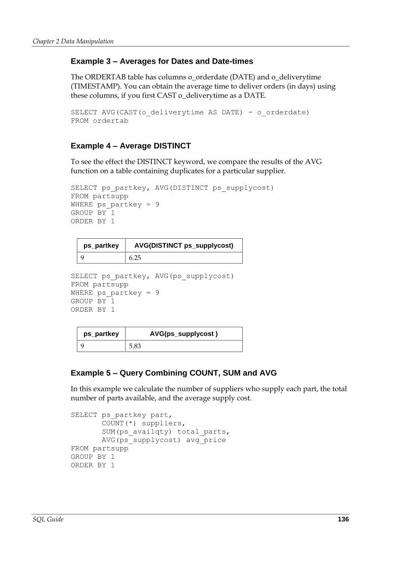
Chapter 2 Data Manipulation
SQL Guide 136
Example 3 – Averages for Dates and Date-times
The ORDERTAB table has columns o_orderdate (DATE) and o_deliverytime (TIMESTAMP). You can obtain the average time to deliver orders (in days) using these columns, if you first CAST o_deliverytime as a DATE.
SELECT AVG(CAST(o_deliverytime AS DATE) - o_orderdate)
FROM ordertab
Example 4 – Average DISTINCT
To see the effect the DISTINCT keyword, we compare the results of the AVG function on a table containing duplicates for a particular supplier.
SELECT ps_partkey, AVG(DISTINCT ps_supplycost)
FROM partsupp
WHERE ps_partkey = 9
GROUP BY 1
ORDER BY 1
ps_partkey AVG(DISTINCT ps_supplycost)
9 6.25
SELECT ps_partkey, AVG(ps_supplycost)
FROM partsupp
WHERE ps_partkey = 9
GROUP BY 1
ORDER BY 1
ps_partkey AVG(ps_supplycost )
9 5.83
Example 5 – Query Combining COUNT, SUM and AVG
In this example we calculate the number of suppliers who supply each part, the total number of parts available, and the average supply cost.
SELECT ps_partkey part,
COUNT(*) suppliers,
SUM(ps_availqty) total_parts,
AVG(ps_supplycost) avg_price
FROM partsupp
GROUP BY 1
ORDER BY 1
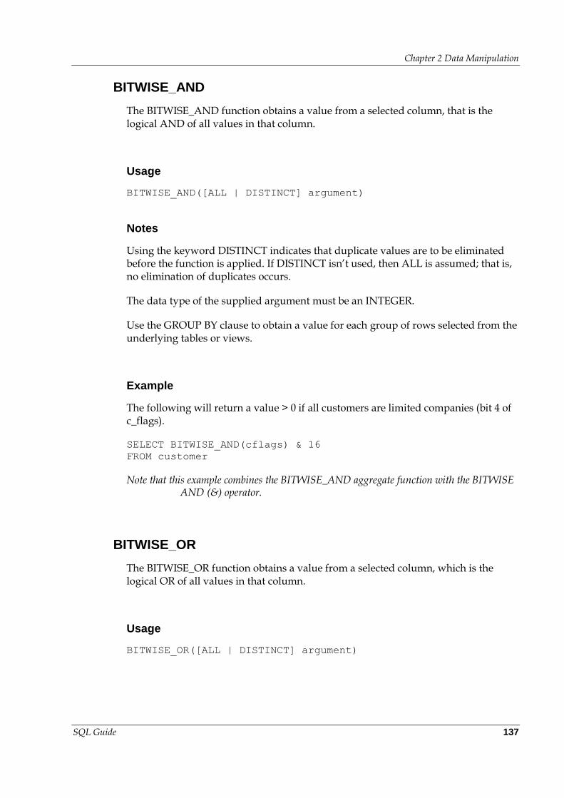
Chapter 2 Data Manipulation
SQL Guide 137
BITWISE_AND
The BITWISE_AND function obtains a value from a selected column, that is the logical AND of all values in that column.
Usage
BITWISE_AND([ALL | DISTINCT] argument)
Notes
Using the keyword DISTINCT indicates that duplicate values are to be eliminated before the function is applied. If DISTINCT isn’t used, then ALL is assumed; that is, no elimination of duplicates occurs.
The data type of the supplied argument must be an INTEGER.
Use the GROUP BY clause to obtain a value for each group of rows selected from the underlying tables or views.
Example
The following will return a value > 0 if all customers are limited companies (bit 4 of c_flags).
SELECT BITWISE_AND(cflags) & 16
FROM customer
Note that this example combines the BITWISE_AND aggregate function with the BITWISE AND (&) operator.
BITWISE_OR
The BITWISE_OR function obtains a value from a selected column, which is the logical OR of all values in that column.
Usage
BITWISE_OR([ALL | DISTINCT] argument)
Chapter 2 Data Manipulation
SQL Guide 138
Notes
Using the keyword DISTINCT indicates that duplicate values are to be eliminated before the function is applied. If DISTINCT isn’t used, then ALL is assumed; that is, no elimination of duplicates occurs.
The data type of the supplied argument must be an INTEGER.
Use the GROUP BY clause to obtain a value for each group of rows selected from the underlying tables or views.
Example
The following will return a value > 0 if any customers are limited companies (bit 4 of c_flags).
SELECT BITWISE_OR(cflags) & 16
FROM customer
Note that this example combines the BITWISE_OR aggregate function with the BITWISE AND (&) operator.
COUNT
Use the COUNT function to count the number of data values in a selected column. The function always returns an INTEGER that is equal to
The number of rows, or
The number of values in the column.
The data in the column can be of any type.
Use the special function COUNT(*) to count rows.
Usage
COUNT({* | [DISTINCT | ALL] scalar-expression})
Notes
Using the keyword DISTINCT (except in the case of COUNT(*) where it is not allowed), indicates that duplicate values are to be eliminated before the function is applied. If DISTINCT isn’t used, then ALL is assumed; that is, no duplicate elimination.
Chapter 2 Data Manipulation
SQL Guide 139
In the case of COUNT(*), any NULLs encountered are treated just like non-NULL values. If the argument is an empty set (that is, there are no rows), then COUNT(*) returns a value of zero.
Use the GROUP BY clause to create a count for each group of rows selected from the underlying table or view.
Example 1 – COUNT(*)
Determine the number of rows in the PARTSUPP table.
SELECT COUNT(*)
FROM partsupp
Example 2 – COUNT DISTINCT
Count the number of parts in the PARTSUPP table, using DISTINCT to eliminate duplicates.
SELECT COUNT(DISTINCT ps_partkey)
FROM partsupp
Example 3 – GROUP BY
Count the number of parts supplied by each supplier in the PARTSUPP table.
SELECT supplier, COUNT(DISTINCT ps_partkey) part
FROM partsupp
GROUP BY 1
ORDER BY 1
Example 4 – COUNT with a CASE Statement
Do a count with a CASE statement, to find out how many rows match your categories for order size (based on o_totalprice) for the ORDERTAB table.
SELECT
CASE
WHEN o_totalprice = 0 THEN 'no orders'
WHEN o_totalprice BETWEEN 0 AND 100 THEN 'small'
WHEN o_totalprice BETWEEN 101 AND 1000 THEN 'medium'
WHEN o_totalprice BETWEEN 1001 AND 2000 THEN 'large'
ELSE 'very large'
END ordersize,
COUNT (*)
FROM ordertab
GROUP BY 1
ORDER BY 1
Chapter 2 Data Manipulation
SQL Guide 140
MAX
Use the MAX function to obtain the value from a selected column, which is the maximum value in that column.
Usage
MAX([ALL | DISTINCT] scalar-expression)
Notes
Using the keyword DISTINCT is legal but is meaningless with this function.
Any NULLs are eliminated before making the calculation.
Use the GROUP BY clause to create a maximum value for each group of rows selected from the underlying tables or views.
Example 1 – Basic MAX
Determine the largest order placed from the ORDERTAB table.
SELECT MAX(o_totalprice)
FROM ordertab
Now, work out who placed the order. (This requires a sub-query.)
SELECT o_custkey customer, o_totalprice largest_order
FROM ordertab
WHERE o_totalprice = (
SELECT MAX(o_totalprice)
FROM ordertab
)
Example 2 – Using GROUP BY
Calculate the maximum order placed by each customer.
SELECT o_custkey, MAX(o_totalprice)
FROM ordertab
GROUP BY 1
ORDER BY 2 DESC
Chapter 2 Data Manipulation
SQL Guide 141
Example 3 – COUNT, MAX and GROUP BY
This example finds out how many parts are listed for each supplier, and gives the cost of the most expensive item.
SELECT ps_suppkey, COUNT(ps_partkey), MAX(ps_supplycost)
FROM partsupp
GROUP BY 1
ORDER BY 3 DESC
MIN
Use the MIN function to obtain the value from a selected column, which is the minimum value in that column.
Usage
MIN([ALL | DISTINCT] scalar-expression)
Notes
Using the keyword DISTINCT is legal but is meaningless with this function.
Any NULLs are eliminated before making the calculation.
Use the GROUP BY clause to create a minimum for each group of rows selected from the underlying tables or views.
Example 1 – Determine the Smallest Order Placed
Determine the smallest order placed by any customer in the O_ORDERTAB table.
SELECT MIN(o_totalprice)
FROM ordertab
Example 2 – MIN and MAX Prices for Parts with Multiple Suppliers
Where more than one supplier supplies a part, display the maximum and minimum prices.
SELECT ps_partkey part,
MIN(ps_supplycost) min_cost,
MAX(ps_supplycost) max_cost
FROM partsupp
GROUP BY 1
HAVING COUNT(*) > 1
ORDER BY 1
Chapter 2 Data Manipulation
SQL Guide 142
STDEV
Standard Deviation is calculated as the square root of the variance of the argument, and consequently is subject to the same constraints as VAR.
Usage
SDEV(argument)
STDEV(argument)
STDDEV(argument)
Notes
The three forms only differ in their spelling.
SUM
The SUM function obtains a value from a selected column, which is the sum of all values in that column.
Usage
SUM([ALL | DISTINCT] scalar-expression)
Notes
Using the keyword DISTINCT indicates that duplicate values are to be eliminated before the function is applied. If DISTINCT isn’t used, then ALL is assumed; that is, no elimination of duplicates occurs.
For this function, the argument must be of numeric type, and NULLs are not included in the result calculation.
Use the GROUP BY clause to create a sum for each group of rows selected from the underlying tables or views.
To reduce the possibility an overflow resulting from an aggregation, INTEGER values are coerced into INT8.
Chapter 2 Data Manipulation
SQL Guide 143
Example 1 – Value of Orders Placed
Using the ORDERTAB table, determine the total value of orders placed.
SELECT COUNT(o_totalprice), SUM(o_totalprice)
FROM ordertab
Example 2 – Supplier Name and Total Stock Value
Display the supplier name and the total value of their stock for those suppliers who supply at least 5 items and where the value of the stock is over £3000.
SELECT s_name,
SUM(ps_availqty * ps_supplycost) AS value_of_stock
FROM partsupp, supplier
WHERE s_suppkey = ps_suppkey
GROUP BY 1
HAVING COUNT(ps_partkey) >= 5 AND
SUM(ps_availqty * ps_supplycost) > 3000.00
ORDER BY 2 DESC
VAR
Returns variance of a column.
Usage
VAR(argument)
Notes
The argument for VAR must be numeric. The result has a FLOAT data type, and is generated by determining the variance of the underlying result set. This is an aggregate operation and as such may require a GROUP BY clause. It cannot be used in a WHERE clause. An error occurs if the argument has an invalid data type, or if the calculation generates any result (final or intermediate) that is too large to be represented by a FLOAT.
FILTER Clauses
FILTER clauses are specified in the SQL2012 specification; they effectively allow different WHERE clauses to be applied to different aggregate functions in a single SELECT statement.
Chapter 2 Data Manipulation
SQL Guide 144
Usage
aggregate-function(function-arguments) [filter (where-clause)]
Notes
A FILTER clause cannot contain a query expression, a window function, or an outer reference.
Example
SELECT
COUNT(o_orderkey) FILTER (WHERE o_orderstatus = '0'),
SUM(o_totalprice) FILTER (WHERE o_totalprice > 100),
MAX(o_deliverytime) FILTER (WHERE o_orderprioriy <> 'low')
FROM ordertab
ANY, EVERY and SOME
ANY, EVERY, and SOME can be used in the HAVING clause of aggregate functions.
Usage
HAVING {ANY | EVERY | SOME} (predicate)
Notes
ANY and SOME must match at least one row in the group. EVERY must match all rows in the group.
Example
The following query return all ps_suppkey values where ps_supplycost is always less that 100 for that value of ps_suppkey.
SELECT ps_suppkey
FROM partsupp
GROUP BY 1
HAVING EVERY(ps_supplycost < 100.00)
ORDER BY 1
2.9 Binary Aggregate Functions
Binary aggregate functions perform a variety of regression and correlation analysis.
Chapter 2 Data Manipulation
SQL Guide 145
Usage
function-name(independent-parameter, dependent-parameter)
Notes
function-name denotes the binary aggregate function name.
The binary aggregate functions take a pair of arguments, the independent-variable-expression and the dependent-variable-expression, which are both a numeric-value-expression.
Any row in which either argument evaluates to NULL is removed from the group. If there are no rows remaining in the group and the function-name is REGR_COUNT then the result is 0; the other binary aggregate functions will return a result of NULL. Otherwise, the computation concludes and the result is dependent on the binary aggregate function.
Kognitio supports the following binary aggregate functions:
Function Description
REGR_COUNT The number of rows remaining in the group
REGR_SXX The sum of squares of the independent-variable-expression
REGR_SYY The sum of squares of the dependent-variable-expression
REGR_SXY The sum of products of independent-variable-expression times dependent-variable-expression
REGR_AVGX The average of independent-variable-expression
REGR_AVGY The average of dependent-variable-expression
COVAR_POP The population covariance; defined as the sum of products of the difference of independent-variable-expression from its mean times the difference of dependent-variable-expression from its mean, divided by the number of rows remaining
COVAR_SAMP The sample covariance; defined as the sum of products of the difference of independent-variable-expression from its mean times the difference of dependent-variable-expression from its mean, divided by the number of rows remaining minus 1
CORR The correlation coefficient; defined as the ratio of the population covariance divided by the product of the population standard deviation of independent-variable-expression and the population standard deviation of dependent-variable-expression
REGR_R2 The square of the correlation coefficient
REGR_SLOPE The slope of the least-squares-fit linear equation determined by the (independent-variable-expression, dependent-variable-expression) pairs
REGR_INTERCEPT The y-intercept of the least-squares-fit linear equation determined by the (independent-variable-expression, dependent-variable-expression) pairs
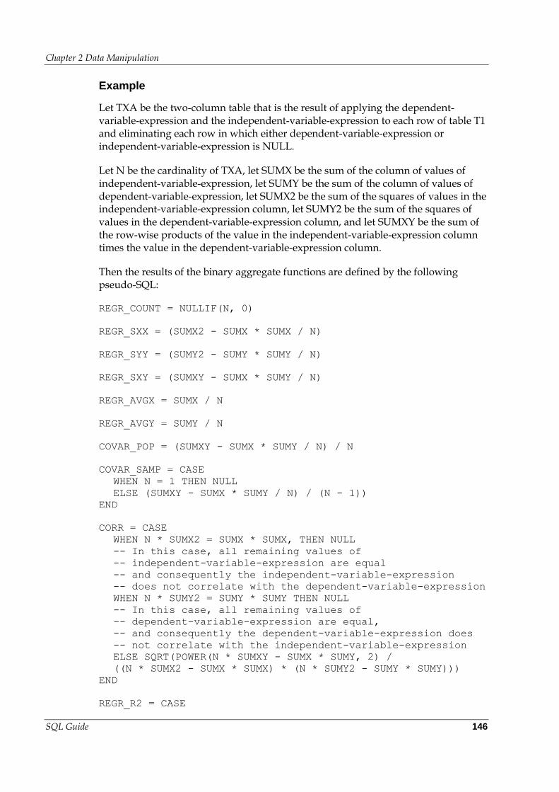
Chapter 2 Data Manipulation
SQL Guide 146
Example
Let TXA be the two-column table that is the result of applying the dependent-variable-expression and the independent-variable-expression to each row of table T1 and eliminating each row in which either dependent-variable-expression or independent-variable-expression is NULL.
Let N be the cardinality of TXA, let SUMX be the sum of the column of values of independent-variable-expression, let SUMY be the sum of the column of values of dependent-variable-expression, let SUMX2 be the sum of the squares of values in the independent-variable-expression column, let SUMY2 be the sum of the squares of values in the dependent-variable-expression column, and let SUMXY be the sum of the row-wise products of the value in the independent-variable-expression column times the value in the dependent-variable-expression column.
Then the results of the binary aggregate functions are defined by the following pseudo-SQL:
REGR_COUNT = NULLIF(N, 0)
REGR_SXX = (SUMX2 - SUMX * SUMX / N)
REGR_SYY = (SUMY2 - SUMY * SUMY / N)
REGR_SXY = (SUMXY - SUMX * SUMY / N)
REGR_AVGX = SUMX / N
REGR_AVGY = SUMY / N
COVAR_POP = (SUMXY - SUMX * SUMY / N) / N
COVAR_SAMP = CASE
WHEN N = 1 THEN NULL
ELSE (SUMXY - SUMX * SUMY / N) / (N - 1))
END
CORR = CASE
WHEN N * SUMX2 = SUMX * SUMX, THEN NULL
-- In this case, all remaining values of
-- independent-variable-expression are equal
-- and consequently the independent-variable-expression
-- does not correlate with the dependent-variable-expression
WHEN N * SUMY2 = SUMY * SUMY THEN NULL
-- In this case, all remaining values of
-- dependent-variable-expression are equal,
-- and consequently the dependent-variable-expression does
-- not correlate with the independent-variable-expression
ELSE SQRT(POWER(N * SUMXY - SUMX * SUMY, 2) /
((N * SUMX2 - SUMX * SUMX) * (N * SUMY2 - SUMY * SUMY)))
END
REGR_R2 = CASE
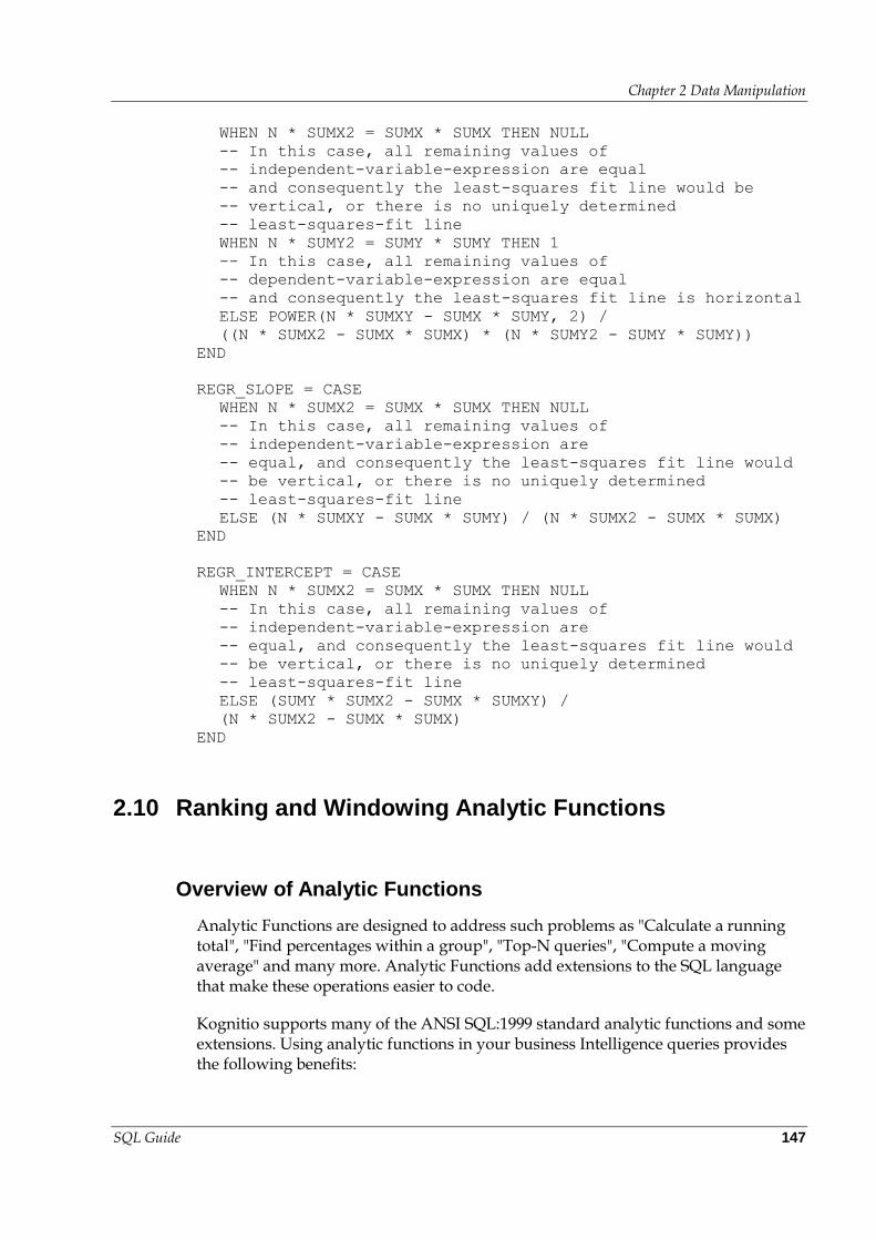
Chapter 2 Data Manipulation
SQL Guide 147
WHEN N * SUMX2 = SUMX * SUMX THEN NULL
-- In this case, all remaining values of
-- independent-variable-expression are equal
-- and consequently the least-squares fit line would be
-- vertical, or there is no uniquely determined
-- least-squares-fit line
WHEN N * SUMY2 = SUMY * SUMY THEN 1
-- In this case, all remaining values of
-- dependent-variable-expression are equal
-- and consequently the least-squares fit line is horizontal
ELSE POWER(N * SUMXY - SUMX * SUMY, 2) /
((N * SUMX2 - SUMX * SUMX) * (N * SUMY2 - SUMY * SUMY))
END
REGR_SLOPE = CASE
WHEN N * SUMX2 = SUMX * SUMX THEN NULL
-- In this case, all remaining values of
-- independent-variable-expression are
-- equal, and consequently the least-squares fit line would
-- be vertical, or there is no uniquely determined
-- least-squares-fit line
ELSE (N * SUMXY - SUMX * SUMY) / (N * SUMX2 - SUMX * SUMX)
END
REGR_INTERCEPT = CASE
WHEN N * SUMX2 = SUMX * SUMX THEN NULL
-- In this case, all remaining values of
-- independent-variable-expression are
-- equal, and consequently the least-squares fit line would
-- be vertical, or there is no uniquely determined
-- least-squares-fit line
ELSE (SUMY * SUMX2 - SUMX * SUMXY) /
(N * SUMX2 - SUMX * SUMX)
END
2.10 Ranking and Windowing Analytic Functions
Overview of Analytic Functions
Analytic Functions are designed to address such problems as "Calculate a running total", "Find percentages within a group", "Top-N queries", "Compute a moving average" and many more. Analytic Functions add extensions to the SQL language that make these operations easier to code.
Kognitio supports many of the ANSI SQL:1999 standard analytic functions and some extensions. Using analytic functions in your business Intelligence queries provides the following benefits:
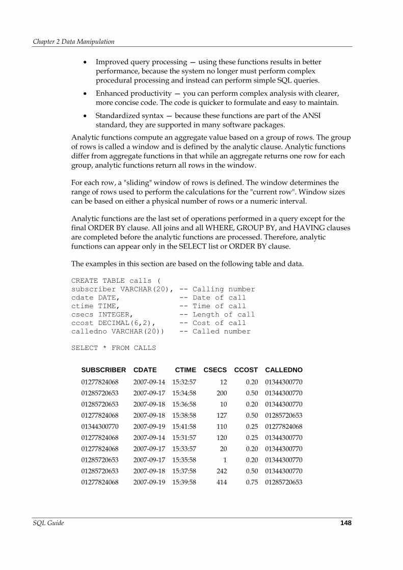
Chapter 2 Data Manipulation
SQL Guide 148
Improved query processing — using these functions results in better performance, because the system no longer must perform complex procedural processing and instead can perform simple SQL queries.
Enhanced productivity — you can perform complex analysis with clearer, more concise code. The code is quicker to formulate and easy to maintain.
Standardized syntax — because these functions are part of the ANSI standard, they are supported in many software packages.
Analytic functions compute an aggregate value based on a group of rows. The group of rows is called a window and is defined by the analytic clause. Analytic functions differ from aggregate functions in that while an aggregate returns one row for each group, analytic functions return all rows in the window.
For each row, a "sliding" window of rows is defined. The window determines the range of rows used to perform the calculations for the "current row". Window sizes can be based on either a physical number of rows or a numeric interval.
Analytic functions are the last set of operations performed in a query except for the final ORDER BY clause. All joins and all WHERE, GROUP BY, and HAVING clauses are completed before the analytic functions are processed. Therefore, analytic functions can appear only in the SELECT list or ORDER BY clause.
The examples in this section are based on the following table and data.
CREATE TABLE calls (
subscriber VARCHAR(20), -- Calling number
cdate DATE, -- Date of call
ctime TIME, -- Time of call
csecs INTEGER, -- Length of call
ccost DECIMAL(6,2), -- Cost of call
calledno VARCHAR(20)) -- Called number
SELECT * FROM CALLS
SUBSCRIBER CDATE CTIME CSECS CCOST CALLEDNO
01277824068 2007-09-14 15:32:57 12 0.20 01344300770
01285720653 2007-09-17 15:34:58 200 0.50 01344300770
01285720653 2007-09-18 15:36:58 10 0.20 01344300770
01277824068 2007-09-18 15:38:58 127 0.50 01285720653
01344300770 2007-09-19 15:41:58 110 0.25 01277824068
01277824068 2007-09-14 15:31:57 120 0.25 01344300770
01277824068 2007-09-17 15:33:57 20 0.20 01344300770
01285720653 2007-09-17 15:35:58 1 0.20 01344300770
01285720653 2007-09-18 15:37:58 242 0.50 01344300770
01277824068 2007-09-19 15:39:58 414 0.75 01285720653
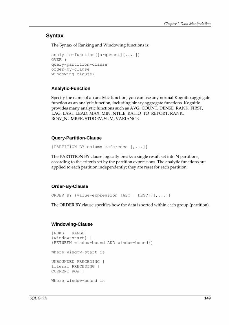
Chapter 2 Data Manipulation
SQL Guide 149
Syntax
The Syntax of Ranking and Windowing functions is:
analytic-function([argument][,...])
OVER (
query-partition-clause
order-by-clause
windowing-clause)
Analytic-Function
Specify the name of an analytic function; you can use any normal Kognitio aggregate function as an analytic function, including binary aggregate functions. Kognitio provides many analytic functions such as AVG, COUNT, DENSE_RANK, FIRST, LAG, LAST, LEAD, MAX, MIN, NTILE, RATIO_TO_REPORT, RANK, ROW_NUMBER, STDDEV, SUM, VARIANCE.
Query-Partition-Clause
[PARTITION BY column-reference [,...]]
The PARTITION BY clause logically breaks a single result set into N partitions, according to the criteria set by the partition expressions. The analytic functions are applied to each partition independently; they are reset for each partition.
Order-By-Clause
ORDER BY {value-expression [ASC | DESC]}[,...]]
The ORDER BY clause specifies how the data is sorted within each group (partition).
Windowing-Clause
[ROWS | RANGE
{window-start} |
{BETWEEN window-bound AND window-bound}]
Where window-start is
UNBOUNDED PRECEDING |
literal PRECEDING |
CURRENT ROW |
Where window-bound is
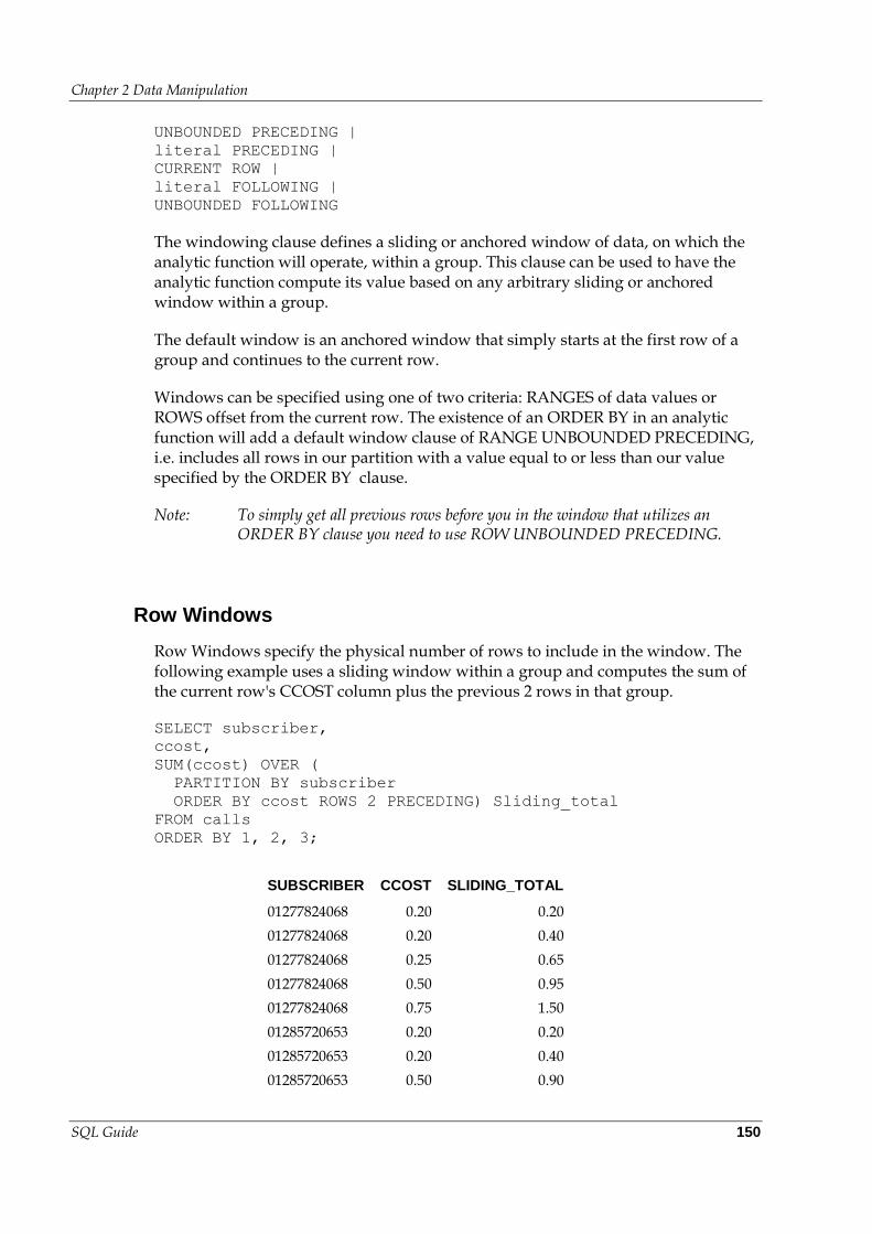
Chapter 2 Data Manipulation
SQL Guide 150
UNBOUNDED PRECEDING |
literal PRECEDING |
CURRENT ROW |
literal FOLLOWING |
UNBOUNDED FOLLOWING
The windowing clause defines a sliding or anchored window of data, on which the analytic function will operate, within a group. This clause can be used to have the analytic function compute its value based on any arbitrary sliding or anchored window within a group.
The default window is an anchored window that simply starts at the first row of a group and continues to the current row.
Windows can be specified using one of two criteria: RANGES of data values or ROWS offset from the current row. The existence of an ORDER BY in an analytic function will add a default window clause of RANGE UNBOUNDED PRECEDING, i.e. includes all rows in our partition with a value equal to or less than our value specified by the ORDER BY clause.
Note: To simply get all previous rows before you in the window that utilizes an ORDER BY clause you need to use ROW UNBOUNDED PRECEDING.
Row Windows
Row Windows specify the physical number of rows to include in the window. The following example uses a sliding window within a group and computes the sum of the current row's CCOST column plus the previous 2 rows in that group.
SELECT subscriber,
ccost,
SUM(ccost) OVER (
PARTITION BY subscriber
ORDER BY ccost ROWS 2 PRECEDING) Sliding_total
FROM calls
ORDER BY 1, 2, 3;
SUBSCRIBER CCOST SLIDING_TOTAL
01277824068 0.20 0.20
01277824068 0.20 0.40
01277824068 0.25 0.65
01277824068 0.50 0.95
01277824068 0.75 1.50
01285720653 0.20 0.20
01285720653 0.20 0.40
01285720653 0.50 0.90
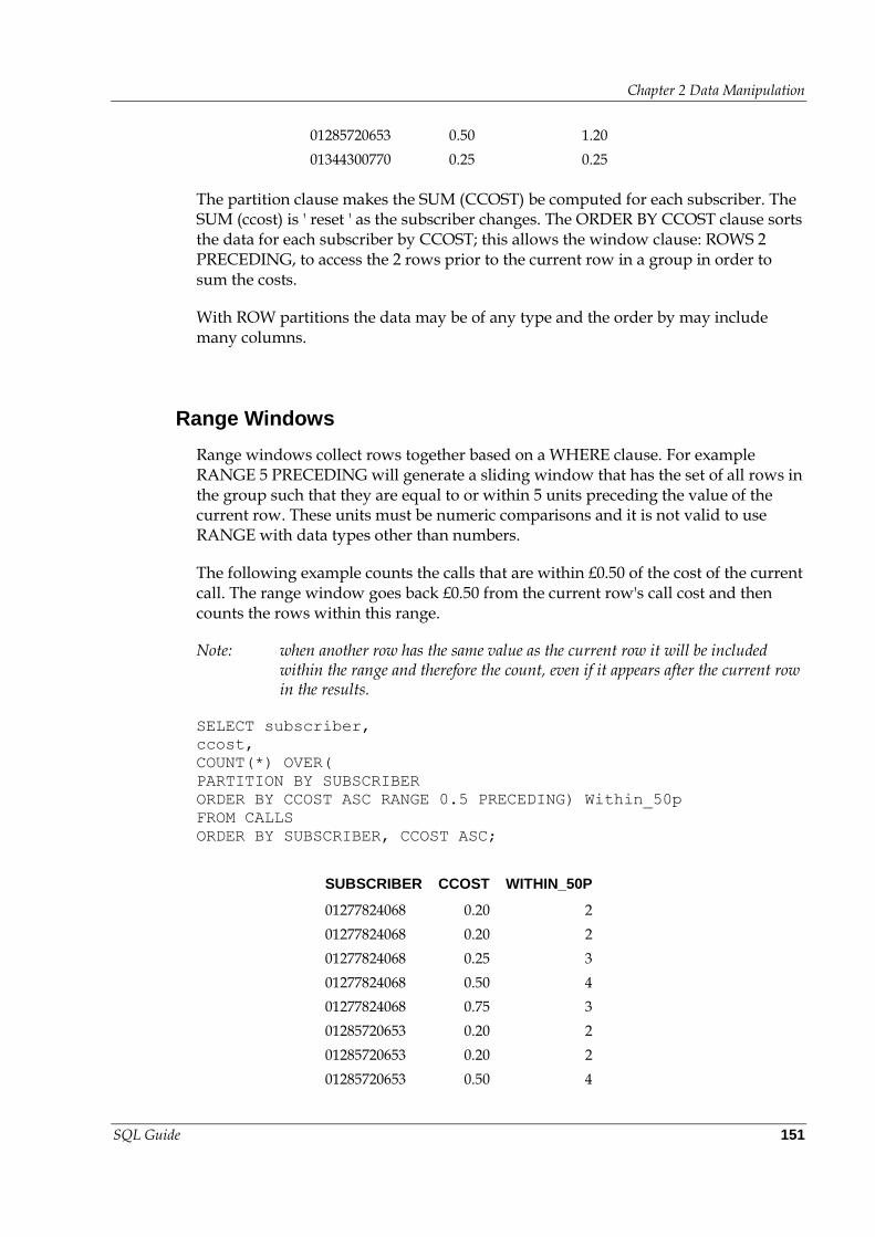
Chapter 2 Data Manipulation
SQL Guide 151
01285720653 0.50 1.20
01344300770 0.25 0.25
The partition clause makes the SUM (CCOST) be computed for each subscriber. The SUM (ccost) is ' reset ' as the subscriber changes. The ORDER BY CCOST clause sorts the data for each subscriber by CCOST; this allows the window clause: ROWS 2 PRECEDING, to access the 2 rows prior to the current row in a group in order to sum the costs.
With ROW partitions the data may be of any type and the order by may include many columns.
Range Windows
Range windows collect rows together based on a WHERE clause. For example RANGE 5 PRECEDING will generate a sliding window that has the set of all rows in the group such that they are equal to or within 5 units preceding the value of the current row. These units must be numeric comparisons and it is not valid to use RANGE with data types other than numbers.
The following example counts the calls that are within £0.50 of the cost of the current call. The range window goes back £0.50 from the current row's call cost and then counts the rows within this range.
Note: when another row has the same value as the current row it will be included within the range and therefore the count, even if it appears after the current row in the results.
SELECT subscriber,
ccost,
COUNT(*) OVER(
PARTITION BY SUBSCRIBER
ORDER BY CCOST ASC RANGE 0.5 PRECEDING) Within_50p
FROM CALLS
ORDER BY SUBSCRIBER, CCOST ASC;
SUBSCRIBER CCOST WITHIN_50P
01277824068 0.20 2
01277824068 0.20 2
01277824068 0.25 3
01277824068 0.50 4
01277824068 0.75 3
01285720653 0.20 2
01285720653 0.20 2
01285720653 0.50 4

Chapter 2 Data Manipulation
SQL Guide 152
01285720653 0.50 4
01344300770 0.25 1
Running Totals
This example shows how to calculate a "Running Total" for the entire query. This is done using the entire ordered result set. In addition we compute a running total for each subscriber.
SELECT subscriber, cdate, ctime, ccost,
SUM(ccost) OVER(
ORDER BY cdate, ctime) rtot,
SUM(ccost) OVER(
PARTITION BY subscriber
ORDER BY cdate, ctime) AS subtot
FROM calls
ORDER BY rtot
SUBSCRIBER CDATE CTIME CCOST RTOT SUBTOT
01277824068 2007-09-14 15:31:57 0.25 0.25 0.25
01277824068 2007-09-14 15:32:57 0.20 0.45 0.45
01277824068 2007-09-17 15:33:57 0.20 0.65 0.65
01285720653 2007-09-17 15:34:58 0.50 1.15 0.50
01285720653 2007-09-17 15:35:58 0.20 1.35 0.70
01285720653 2007-09-18 15:36:58 0.20 1.55 0.90
01285720653 2007-09-18 15:37:58 0.50 2.05 1.40
01277824068 2007-09-18 15:38:58 0.50 2.55 1.15
01277824068 2007-09-19 15:39:58 0.75 3.30 1.90
01344300770 2007-09-19 15:41:58 0.25 3.55 0.25
LAG and LEAD: Accessing Rows around the Current Row
Frequently you want to access data not only from the current row but the also the previous or next row. For example, the following query shows the details of the current call and the date of the previous call made by the subscriber.
SELECT subscriber, cdate, ctime,
LAG(cdate, 1) OVER(
PARTITION BY subscriber
ORDER BY cdate, ctime) prev_call
FROM CALLS
ORDER BY 1, 2, 3
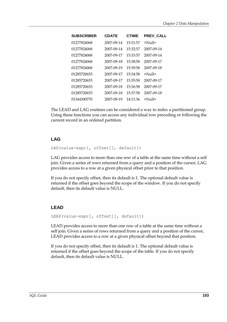
Chapter 2 Data Manipulation
SQL Guide 153
SUBSCRIBER CDATE CTIME PREV_CALL
01277824068 2007-09-14 15:31:57 <Null>
01277824068 2007-09-14 15:32:57 2007-09-14
01277824068 2007-09-17 15:33:57 2007-09-14
01277824068 2007-09-18 15:38:58 2007-09-17
01277824068 2007-09-19 15:39:58 2007-09-18
01285720653 2007-09-17 15:34:58 <Null>
01285720653 2007-09-17 15:35:58 2007-09-17
01285720653 2007-09-18 15:36:58 2007-09-17
01285720653 2007-09-18 15:37:58 2007-09-18
01344300770 2007-09-19 14:11:36 <Null>
The LEAD and LAG routines can be considered a way to index a partitioned group. Using these functions you can access any individual row preceding or following the current record in an ordered partition.
LAG
LAG(value-expr[, offset][, default])
LAG provides access to more than one row of a table at the same time without a self join. Given a series of rows returned from a query and a position of the cursor, LAG provides access to a row at a given physical offset prior to that position.
If you do not specify offset, then its default is 1. The optional default value is returned if the offset goes beyond the scope of the window. If you do not specify default, then its default value is NULL.
LEAD
LEAD(value-expr[, offset][, default])
LEAD provides access to more than one row of a table at the same time without a self join. Given a series of rows returned from a query and a position of the cursor, LEAD provides access to a row at a given physical offset beyond that position.
If you do not specify offset, then its default is 1. The optional default value is returned if the offset goes beyond the scope of the table. If you do not specify default, then its default value is NULL.
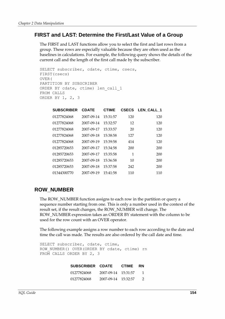
Chapter 2 Data Manipulation
SQL Guide 154
FIRST and LAST: Determine the First/Last Value of a Group
The FIRST and LAST functions allow you to select the first and last rows from a group. These rows are especially valuable because they are often used as the baselines in calculations. For example, the following query shows the details of the current call and the length of the first call made by the subscriber.
SELECT subscriber, cdate, ctime, csecs,
FIRST(csecs)
OVER(
PARTITION BY SUBSCRIBER
ORDER BY cdate, ctime) len_call_1
FROM CALLS
ORDER BY 1, 2, 3
SUBSCRIBER CDATE CTIME CSECS LEN_CALL_1
01277824068 2007-09-14 15:31:57 120 120
01277824068 2007-09-14 15:32:57 12 120
01277824068 2007-09-17 15:33:57 20 120
01277824068 2007-09-18 15:38:58 127 120
01277824068 2007-09-19 15:39:58 414 120
01285720653 2007-09-17 15:34:58 200 200
01285720653 2007-09-17 15:35:58 1 200
01285720653 2007-09-18 15:36:58 10 200
01285720653 2007-09-18 15:37:58 242 200
01344300770 2007-09-19 15:41:58 110 110
ROW_NUMBER
The ROW_NUMBER function assigns to each row in the partition or query a sequence number starting from one. This is only a number used in the context of the result set, if the result changes, the ROW_NUMBER will change. The ROW_NUMBER expression takes an ORDER BY statement with the column to be used for the row count with an OVER operator.
The following example assigns a row number to each row according to the date and time the call was made. The results are also ordered by the call date and time.
SELECT subscriber, cdate, ctime,
ROW_NUMBER() OVER(ORDER BY cdate, ctime) rn
FROM CALLS ORDER BY 2, 3
SUBSCRIBER CDATE CTIME RN
01277824068 2007-09-14 15:31:57 1
01277824068 2007-09-14 15:32:57 2
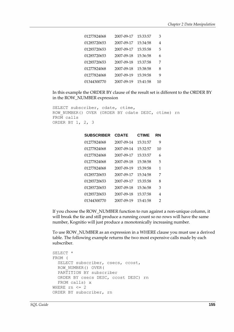
Chapter 2 Data Manipulation
SQL Guide 155
01277824068 2007-09-17 15:33:57 3
01285720653 2007-09-17 15:34:58 4
01285720653 2007-09-17 15:35:58 5
01285720653 2007-09-18 15:36:58 6
01285720653 2007-09-18 15:37:58 7
01277824068 2007-09-18 15:38:58 8
01277824068 2007-09-19 15:39:58 9
01344300770 2007-09-19 15:41:58 10
In this example the ORDER BY clause of the result set is different to the ORDER BY in the ROW_NUMBER expression
SELECT subscriber, cdate, ctime,
ROW_NUMBER() OVER (ORDER BY cdate DESC, ctime) rn
FROM calls
ORDER BY 1, 2, 3
SUBSCRIBER CDATE CTIME RN
01277824068 2007-09-14 15:31:57 9
01277824068 2007-09-14 15:32:57 10
01277824068 2007-09-17 15:33:57 6
01277824068 2007-09-18 15:38:58 5
01277824068 2007-09-19 15:39:58 1
01285720653 2007-09-17 15:34:58 7
01285720653 2007-09-17 15:35:58 8
01285720653 2007-09-18 15:36:58 3
01285720653 2007-09-18 15:37:58 4
01344300770 2007-09-19 15:41:58 2
If you choose the ROW_NUMBER function to run against a non-unique column, it will break the tie and still produce a running count so no rows will have the same number, Kognitio will just produce a monotonically increasing number.
To use ROW_NUMBER as an expression in a WHERE clause you must use a derived table. The following example returns the two most expensive calls made by each subscriber.
SELECT *
FROM (
SELECT subscriber, csecs, ccost,
ROW_NUMBER() OVER(
PARTITION BY subscriber
ORDER BY csecs DESC, ccost DESC) rn
FROM calls) x
WHERE rn <= 2
ORDER BY subscriber, rn
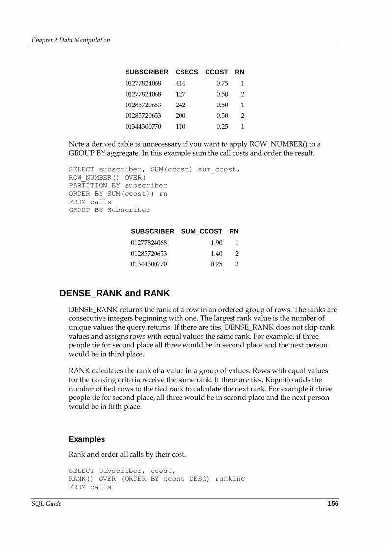
Chapter 2 Data Manipulation
SQL Guide 156
SUBSCRIBER CSECS CCOST RN
01277824068 414 0.75 1
01277824068 127 0.50 2
01285720653 242 0.50 1
01285720653 200 0.50 2
01344300770 110 0.25 1
Note a derived table is unnecessary if you want to apply ROW_NUMBER() to a GROUP BY aggregate. In this example sum the call costs and order the result.
SELECT subscriber, SUM(ccost) sum_ccost,
ROW_NUMBER() OVER(
PARTITION BY subscriber
ORDER BY SUM(ccost)) rn
FROM calls
GROUP BY Subscriber
SUBSCRIBER SUM_CCOST RN
01277824068 1.90 1
01285720653 1.40 2
01344300770 0.25 3
DENSE_RANK and RANK
DENSE_RANK returns the rank of a row in an ordered group of rows. The ranks are consecutive integers beginning with one. The largest rank value is the number of unique values the query returns. If there are ties, DENSE_RANK does not skip rank values and assigns rows with equal values the same rank. For example, if three people tie for second place all three would be in second place and the next person would be in third place.
RANK calculates the rank of a value in a group of values. Rows with equal values for the ranking criteria receive the same rank. If there are ties, Kognitio adds the number of tied rows to the tied rank to calculate the next rank. For example if three people tie for second place, all three would be in second place and the next person would be in fifth place.
Examples
Rank and order all calls by their cost.
SELECT subscriber, ccost,
RANK() OVER (ORDER BY ccost DESC) ranking
FROM calls
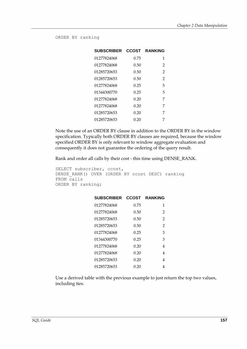
Chapter 2 Data Manipulation
SQL Guide 157
ORDER BY ranking
SUBSCRIBER CCOST RANKING
01277824068 0.75 1
01277824068 0.50 2
01285720653 0.50 2
01285720653 0.50 2
01277824068 0.25 5
01344300770 0.25 5
01277824068 0.20 7
01277824068 0.20 7
01285720653 0.20 7
01285720653 0.20 7
Note the use of an ORDER BY clause in addition to the ORDER BY in the window specification. Typically both ORDER BY clauses are required, because the window specified ORDER BY is only relevant to window aggregate evaluation and consequently it does not guarantee the ordering of the query result.
Rank and order all calls by their cost - this time using DENSE_RANK.
SELECT subscriber, ccost,
DENSE_RANK() OVER (ORDER BY ccost DESC) ranking
FROM calls
ORDER BY ranking;
SUBSCRIBER CCOST RANKING
01277824068 0.75 1
01277824068 0.50 2
01285720653 0.50 2
01285720653 0.50 2
01277824068 0.25 3
01344300770 0.25 3
01277824068 0.20 4
01277824068 0.20 4
01285720653 0.20 4
01285720653 0.20 4
Use a derived table with the previous example to just return the top two values, including ties.
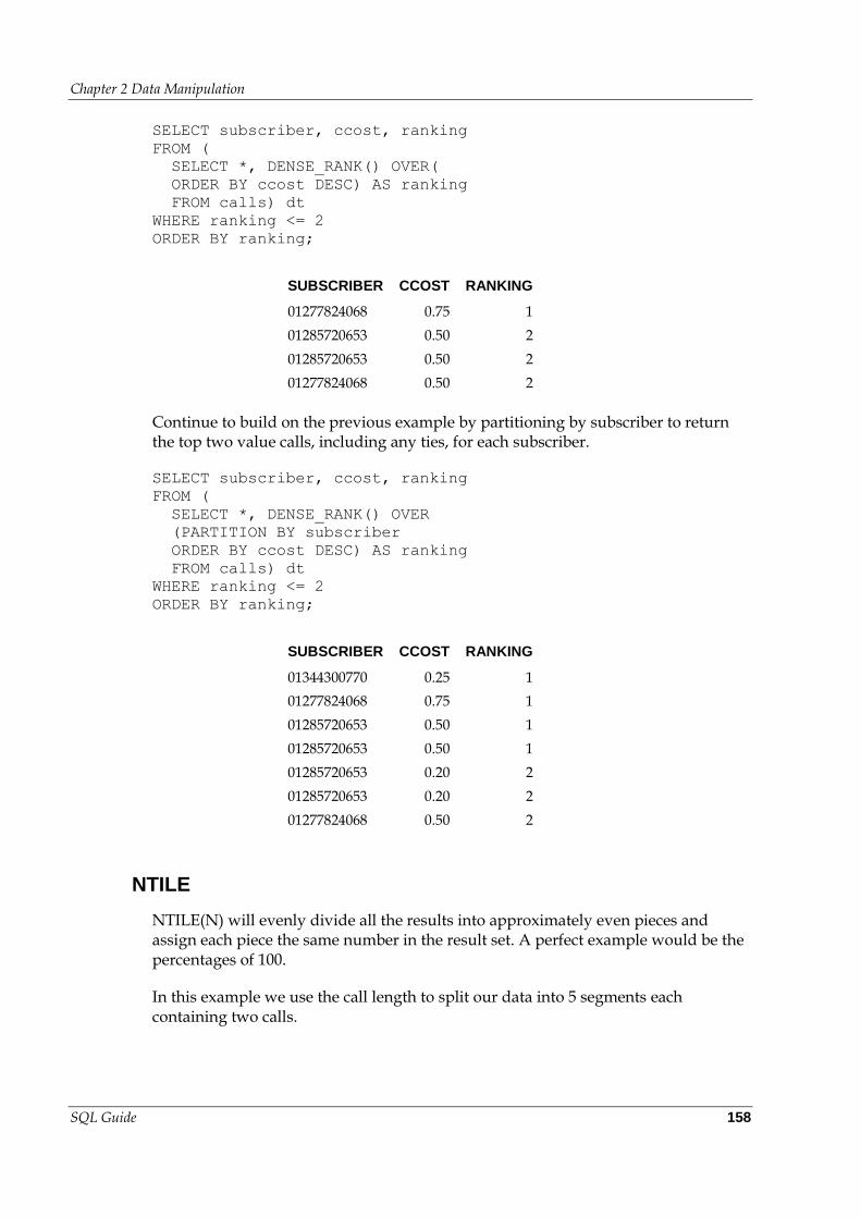
Chapter 2 Data Manipulation
SQL Guide 158
SELECT subscriber, ccost, ranking
FROM (
SELECT *, DENSE_RANK() OVER(
ORDER BY ccost DESC) AS ranking
FROM calls) dt
WHERE ranking <= 2
ORDER BY ranking;
SUBSCRIBER CCOST RANKING
01277824068 0.75 1
01285720653 0.50 2
01285720653 0.50 2
01277824068 0.50 2
Continue to build on the previous example by partitioning by subscriber to return the top two value calls, including any ties, for each subscriber.
SELECT subscriber, ccost, ranking
FROM (
SELECT *, DENSE_RANK() OVER
(PARTITION BY subscriber
ORDER BY ccost DESC) AS ranking
FROM calls) dt
WHERE ranking <= 2
ORDER BY ranking;
SUBSCRIBER CCOST RANKING
01344300770 0.25 1
01277824068 0.75 1
01285720653 0.50 1
01285720653 0.50 1
01285720653 0.20 2
01285720653 0.20 2
01277824068 0.50 2
NTILE
NTILE(N) will evenly divide all the results into approximately even pieces and assign each piece the same number in the result set. A perfect example would be the percentages of 100.
In this example we use the call length to split our data into 5 segments each containing two calls.
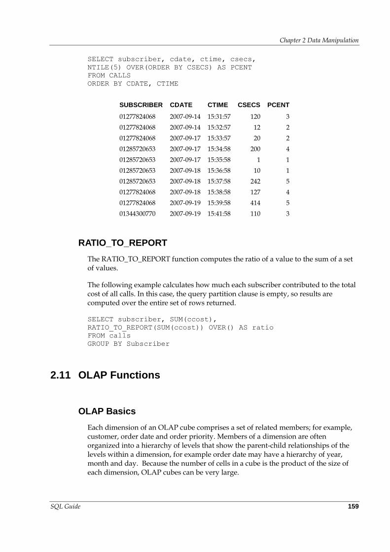
Chapter 2 Data Manipulation
SQL Guide 159
SELECT subscriber, cdate, ctime, csecs,
NTILE(5) OVER(ORDER BY CSECS) AS PCENT
FROM CALLS
ORDER BY CDATE, CTIME
SUBSCRIBER CDATE CTIME CSECS PCENT
01277824068 2007-09-14 15:31:57 120 3
01277824068 2007-09-14 15:32:57 12 2
01277824068 2007-09-17 15:33:57 20 2
01285720653 2007-09-17 15:34:58 200 4
01285720653 2007-09-17 15:35:58 1 1
01285720653 2007-09-18 15:36:58 10 1
01285720653 2007-09-18 15:37:58 242 5
01277824068 2007-09-18 15:38:58 127 4
01277824068 2007-09-19 15:39:58 414 5
01344300770 2007-09-19 15:41:58 110 3
RATIO_TO_REPORT
The RATIO_TO_REPORT function computes the ratio of a value to the sum of a set of values.
The following example calculates how much each subscriber contributed to the total cost of all calls. In this case, the query partition clause is empty, so results are computed over the entire set of rows returned.
SELECT subscriber, SUM(ccost),
RATIO_TO_REPORT(SUM(ccost)) OVER() AS ratio
FROM calls
GROUP BY Subscriber
2.11 OLAP Functions
OLAP Basics
Each dimension of an OLAP cube comprises a set of related members; for example, customer, order date and order priority. Members of a dimension are often organized into a hierarchy of levels that show the parent-child relationships of the levels within a dimension, for example order date may have a hierarchy of year, month and day. Because the number of cells in a cube is the product of the size of each dimension, OLAP cubes can be very large.
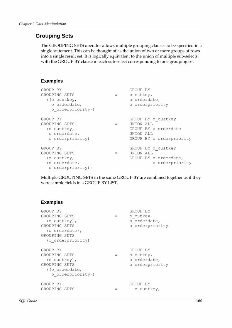
Chapter 2 Data Manipulation
SQL Guide 160
Grouping Sets
The GROUPING SETS operator allows multiple grouping clauses to be specified in a single statement. This can be thought of as the union of two or more groups of rows into a single result set. It is logically equivalent to the union of multiple sub-selects, with the GROUP BY clause in each sub-select corresponding to one grouping set
Examples
GROUP BY
GROUPING SETS
((o_custkey,
o_orderdate,
o_orderpriority))
≡
GROUP BY
o_cutkey,
o_orderdate,
o_orderpriority
GROUP BY
GROUPING SETS
(o_custkey,
o_orderdate,
o_orderpriority)
≡
GROUP BY o_custkey
UNION ALL
GROUP BY o_orderdate
UNION ALL
GROUP BY o_orderpriority
GROUP BY
GROUPING SETS
(o_custkey,
(o_orderdate,
o_orderpriority))
≡
GROUP BY o_custkey
UNION ALL
GROUP BY o_orderdate,
o_orderpriority
Multiple GROUPING SETS in the same GROUP BY are combined together as if they were simple fields in a GROUP BY LIST.
Examples
GROUP BY
GROUPING SETS
(o_custkey),
GROUPING SETS
(o_orderdate),
GROUPING SETS
(o_orderpriority)
≡
GROUP BY
o_cutkey,
o_orderdate,
o_orderpriority
GROUP BY
GROUPING SETS
(o_custkey),
GROUPING SETS
((o_orderdate,
o_orderpriority))
≡
GROUP BY
o_cutkey,
o_orderdate,
o_orderpriority
GROUP BY
GROUPING SETS
≡
GROUP BY
o_custkey,
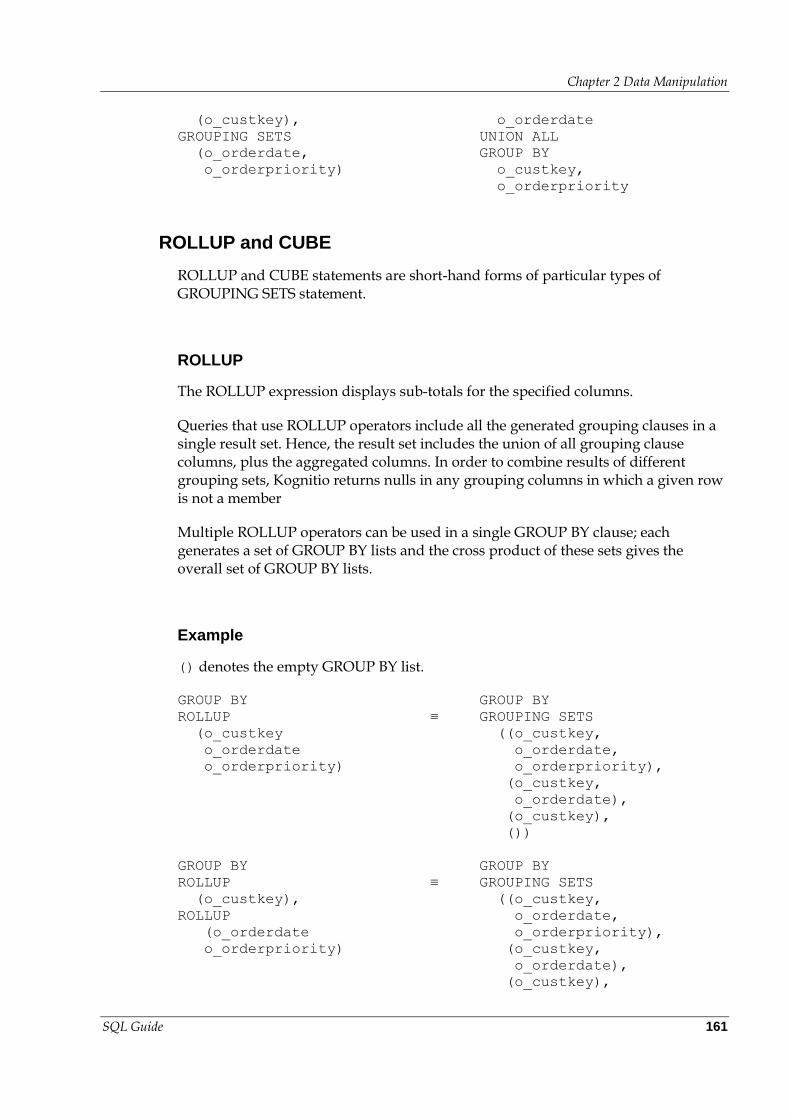
Chapter 2 Data Manipulation
SQL Guide 161
(o_custkey),
GROUPING SETS
(o_orderdate,
o_orderpriority)
o_orderdate
UNION ALL
GROUP BY
o_custkey,
o_orderpriority
ROLLUP and CUBE
ROLLUP and CUBE statements are short-hand forms of particular types of GROUPING SETS statement.
ROLLUP
The ROLLUP expression displays sub-totals for the specified columns.
Queries that use ROLLUP operators include all the generated grouping clauses in a single result set. Hence, the result set includes the union of all grouping clause columns, plus the aggregated columns. In order to combine results of different grouping sets, Kognitio returns nulls in any grouping columns in which a given row is not a member
Multiple ROLLUP operators can be used in a single GROUP BY clause; each generates a set of GROUP BY lists and the cross product of these sets gives the overall set of GROUP BY lists.
Example
() denotes the empty GROUP BY list.
GROUP BY
ROLLUP
(o_custkey
o_orderdate
o_orderpriority)
≡
GROUP BY
GROUPING SETS
((o_custkey,
o_orderdate,
o_orderpriority),
(o_custkey,
o_orderdate),
(o_custkey),
())
GROUP BY
ROLLUP
(o_custkey),
ROLLUP
(o_orderdate
o_orderpriority)
≡
GROUP BY
GROUPING SETS
((o_custkey,
o_orderdate,
o_orderpriority),
(o_custkey,
o_orderdate),
(o_custkey),
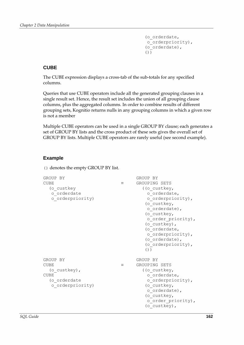
Chapter 2 Data Manipulation
SQL Guide 162
(o_orderdate,
o_orderpriority),
(o_orderdate),
())
CUBE
The CUBE expression displays a cross-tab of the sub-totals for any specified columns.
Queries that use CUBE operators include all the generated grouping clauses in a single result set. Hence, the result set includes the union of all grouping clause columns, plus the aggregated columns. In order to combine results of different grouping sets, Kognitio returns nulls in any grouping columns in which a given row is not a member
Multiple CUBE operators can be used in a single GROUP BY clause; each generates a set of GROUP BY lists and the cross product of these sets gives the overall set of GROUP BY lists. Multiple CUBE operators are rarely useful (see second example).
Example
() denotes the empty GROUP BY list.
GROUP BY
CUBE
(o_custkey
o_orderdate
o_orderpriority)
≡
GROUP BY
GROUPING SETS
((o_custkey,
o_orderdate,
o_orderpriority),
(o_custkey,
o_orderdate),
(o_custkey,
o_order_priority),
(o_custkey),
(o_orderdate,
o_orderpriority),
(o_orderdate),
(o_orderpriority),
())
GROUP BY
CUBE
(o_custkey),
CUBE
(o_orderdate
o_orderpriority)
≡
GROUP BY
GROUPING SETS
((o_custkey,
o_orderdate,
o_orderpriority),
(o_custkey,
o_orderdate),
(o_custkey,
o_order_priority),
(o_custkey),
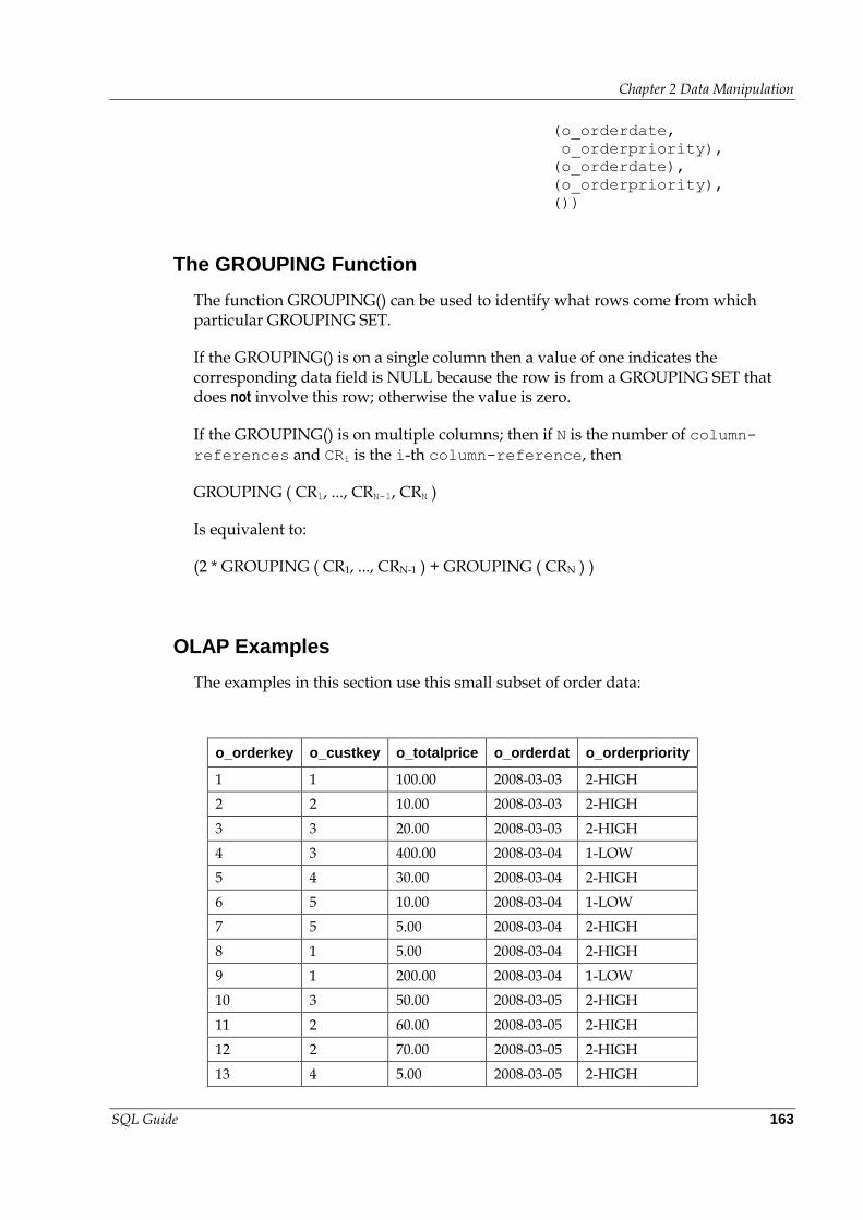
Chapter 2 Data Manipulation
SQL Guide 163
(o_orderdate,
o_orderpriority),
(o_orderdate),
(o_orderpriority),
())
The GROUPING Function
The function GROUPING() can be used to identify what rows come from which particular GROUPING SET.
If the GROUPING() is on a single column then a value of one indicates the corresponding data field is NULL because the row is from a GROUPING SET that does not involve this row; otherwise the value is zero.
If the GROUPING() is on multiple columns; then if N is the number of column-references and CRi is the i-th column-reference, then
GROUPING ( CR1, ..., CRN-1, CRN )
Is equivalent to:
(2 * GROUPING ( CR1, ..., CRN-1 ) + GROUPING ( CRN ) )
OLAP Examples
The examples in this section use this small subset of order data:
o_orderkey o_custkey o_totalprice o_orderdat o_orderpriority
1 1 100.00 2008-03-03 2-HIGH
2 2 10.00 2008-03-03 2-HIGH
3 3 20.00 2008-03-03 2-HIGH
4 3 400.00 2008-03-04 1-LOW
5 4 30.00 2008-03-04 2-HIGH
6 5 10.00 2008-03-04 1-LOW
7 5 5.00 2008-03-04 2-HIGH
8 1 5.00 2008-03-04 2-HIGH
9 1 200.00 2008-03-04 1-LOW
10 3 50.00 2008-03-05 2-HIGH
11 2 60.00 2008-03-05 2-HIGH
12 2 70.00 2008-03-05 2-HIGH
13 4 5.00 2008-03-05 2-HIGH
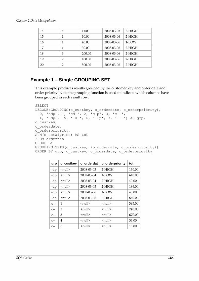
Chapter 2 Data Manipulation
SQL Guide 164
14 4 1.00 2008-03-05 2-HIGH
15 1 10.00 2008-03-06 2-HIGH
16 1 40.00 2008-03-06 1-LOW
17 1 30.00 2008-03-06 2-HIGH
18 3 200.00 2008-03-06 2-HIGH
19 2 100.00 2008-03-06 2-HIGH
20 2 500.00 2008-03-06 2-HIGH
Example 1 – Single GROUPING SET
This example produces results grouped by the customer key and order date and order priority. Note the grouping function is used to indicate which columns have been grouped in each result row.
SELECT
DECODE(GROUPING(o_custkey, o_orderdate, o_orderpriority),
0, 'cdp', 1, 'cd-', 2, 'c-p', 3, 'c--',
4, '-dp', 5, '-d-', 6, '--p', 7, '---') AS grp,
o_custkey,
o_orderdate,
o_orderpriority,
SUM(o_totalprice) AS tot
FROM ordertab
GROUP BY
GROUPING SETS(o_custkey, (o_orderdate, o_orderpriority))
ORDER BY grp, o_custkey, o_orderdate, o_orderpriority
grp o_custkey o_orderdat o_orderpriority tot
-dp <null> 2008-03-03 2-HIGH 130.00
-dp <null> 2008-03-04 1-LOW 610.00
-dp <null> 2008-03-04 2-HIGH 40.00
-dp <null> 2008-03-05 2-HIGH 186.00
-dp <null> 2008-03-06 1-LOW 40.00
-dp <null> 2008-03-06 2-HIGH 840.00
c-- 1 <null> <null> 385.00
c-- 2 <null> <null> 740.00
c-- 3 <null> <null> 670.00
c-- 4 <null> <null> 36.00
c-- 5 <null> <null> 15.00
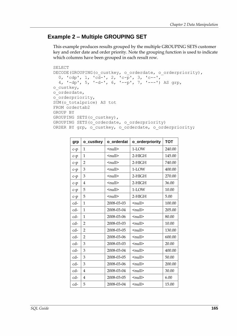
Chapter 2 Data Manipulation
SQL Guide 165
Example 2 – Multiple GROUPING SET
This example produces results grouped by the multiple GROUPING SETS customer key and order date and order priority. Note the grouping function is used to indicate which columns have been grouped in each result row.
SELECT
DECODE(GROUPING(o_custkey, o_orderdate, o_orderpriority),
0, 'cdp', 1, 'cd-', 2, 'c-p', 3, 'c--',
4, '-dp', 5, '-d-', 6, '--p', 7, '---') AS grp,
o_custkey,
o_orderdate,
o_orderpriority,
SUM(o_totalprice) AS tot
FROM ordertab2
GROUP BY
GROUPING SETS(o_custkey),
GROUPING SETS(o_orderdate, o_orderpriority)
ORDER BY grp, o_custkey, o_orderdate, o_orderpriority;
grp o_custkey o_orderdat o_orderpriority TOT
c-p 1 <null> 1-LOW 240.00
c-p 1 <null> 2-HIGH 145.00
c-p 2 <null> 2-HIGH 740.00
c-p 3 <null> 1-LOW 400.00
c-p 3 <null> 2-HIGH 270.00
c-p 4 <null> 2-HIGH 36.00
c-p 5 <null> 1-LOW 10.00
c-p 5 <null> 2-HIGH 5.00
cd- 1 2008-03-03 <null> 100.00
cd- 1 2008-03-04 <null> 205.00
cd- 1 2008-03-06 <null> 80.00
cd- 2 2008-03-03 <null> 10.00
cd- 2 2008-03-05 <null> 130.00
cd- 2 2008-03-06 <null> 600.00
cd- 3 2008-03-03 <null> 20.00
cd- 3 2008-03-04 <null> 400.00
cd- 3 2008-03-05 <null> 50.00
cd- 3 2008-03-06 <null> 200.00
cd- 4 2008-03-04 <null> 30.00
cd- 4 2008-03-05 <null> 6.00
cd- 5 2008-03-04 <null> 15.00
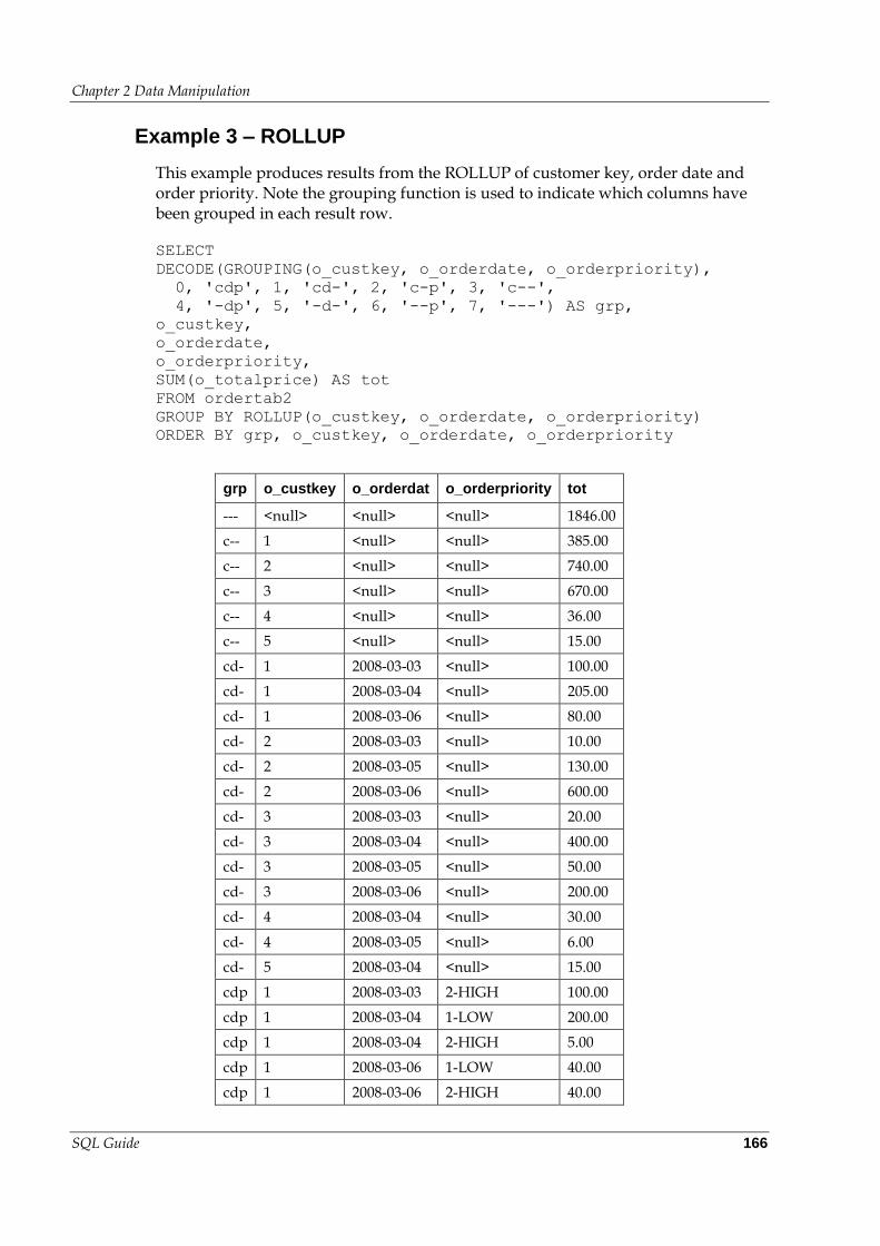
Chapter 2 Data Manipulation
SQL Guide 166
Example 3 – ROLLUP
This example produces results from the ROLLUP of customer key, order date and order priority. Note the grouping function is used to indicate which columns have been grouped in each result row.
SELECT
DECODE(GROUPING(o_custkey, o_orderdate, o_orderpriority),
0, 'cdp', 1, 'cd-', 2, 'c-p', 3, 'c--',
4, '-dp', 5, '-d-', 6, '--p', 7, '---') AS grp,
o_custkey,
o_orderdate,
o_orderpriority,
SUM(o_totalprice) AS tot
FROM ordertab2
GROUP BY ROLLUP(o_custkey, o_orderdate, o_orderpriority)
ORDER BY grp, o_custkey, o_orderdate, o_orderpriority
grp o_custkey o_orderdat o_orderpriority tot
--- <null> <null> <null> 1846.00
c-- 1 <null> <null> 385.00
c-- 2 <null> <null> 740.00
c-- 3 <null> <null> 670.00
c-- 4 <null> <null> 36.00
c-- 5 <null> <null> 15.00
cd- 1 2008-03-03 <null> 100.00
cd- 1 2008-03-04 <null> 205.00
cd- 1 2008-03-06 <null> 80.00
cd- 2 2008-03-03 <null> 10.00
cd- 2 2008-03-05 <null> 130.00
cd- 2 2008-03-06 <null> 600.00
cd- 3 2008-03-03 <null> 20.00
cd- 3 2008-03-04 <null> 400.00
cd- 3 2008-03-05 <null> 50.00
cd- 3 2008-03-06 <null> 200.00
cd- 4 2008-03-04 <null> 30.00
cd- 4 2008-03-05 <null> 6.00
cd- 5 2008-03-04 <null> 15.00
cdp 1 2008-03-03 2-HIGH 100.00
cdp 1 2008-03-04 1-LOW 200.00
cdp 1 2008-03-04 2-HIGH 5.00
cdp 1 2008-03-06 1-LOW 40.00
cdp 1 2008-03-06 2-HIGH 40.00
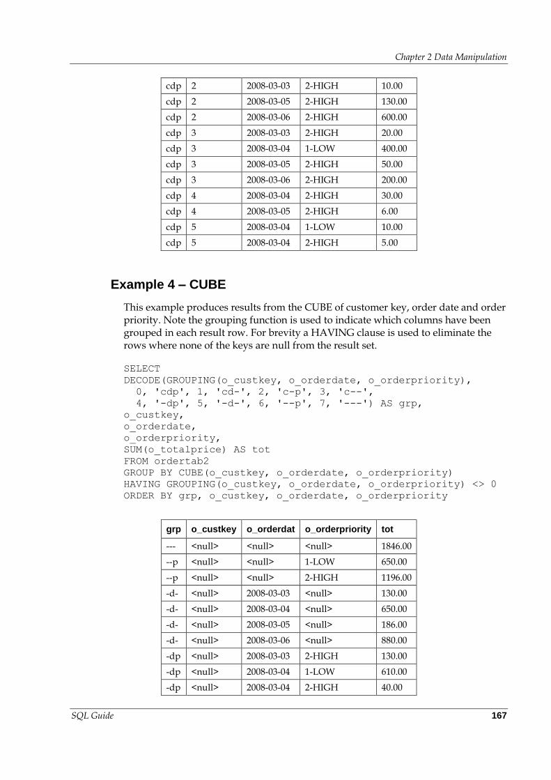
Chapter 2 Data Manipulation
SQL Guide 167
cdp 2 2008-03-03 2-HIGH 10.00
cdp 2 2008-03-05 2-HIGH 130.00
cdp 2 2008-03-06 2-HIGH 600.00
cdp 3 2008-03-03 2-HIGH 20.00
cdp 3 2008-03-04 1-LOW 400.00
cdp 3 2008-03-05 2-HIGH 50.00
cdp 3 2008-03-06 2-HIGH 200.00
cdp 4 2008-03-04 2-HIGH 30.00
cdp 4 2008-03-05 2-HIGH 6.00
cdp 5 2008-03-04 1-LOW 10.00
cdp 5 2008-03-04 2-HIGH 5.00
Example 4 – CUBE
This example produces results from the CUBE of customer key, order date and order priority. Note the grouping function is used to indicate which columns have been grouped in each result row. For brevity a HAVING clause is used to eliminate the rows where none of the keys are null from the result set.
SELECT
DECODE(GROUPING(o_custkey, o_orderdate, o_orderpriority),
0, 'cdp', 1, 'cd-', 2, 'c-p', 3, 'c--',
4, '-dp', 5, '-d-', 6, '--p', 7, '---') AS grp,
o_custkey,
o_orderdate,
o_orderpriority,
SUM(o_totalprice) AS tot
FROM ordertab2
GROUP BY CUBE(o_custkey, o_orderdate, o_orderpriority)
HAVING GROUPING(o_custkey, o_orderdate, o_orderpriority) <> 0
ORDER BY grp, o_custkey, o_orderdate, o_orderpriority
grp o_custkey o_orderdat o_orderpriority tot
--- <null> <null> <null> 1846.00
--p <null> <null> 1-LOW 650.00
--p <null> <null> 2-HIGH 1196.00
-d- <null> 2008-03-03 <null> 130.00
-d- <null> 2008-03-04 <null> 650.00
-d- <null> 2008-03-05 <null> 186.00
-d- <null> 2008-03-06 <null> 880.00
-dp <null> 2008-03-03 2-HIGH 130.00
-dp <null> 2008-03-04 1-LOW 610.00
-dp <null> 2008-03-04 2-HIGH 40.00
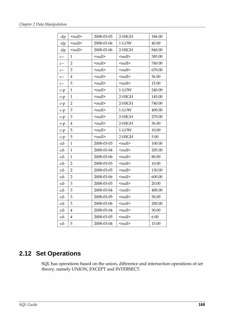
Chapter 2 Data Manipulation
SQL Guide 168
-dp <null> 2008-03-05 2-HIGH 186.00
-dp <null> 2008-03-06 1-LOW 40.00
-dp <null> 2008-03-06 2-HIGH 840.00
c-- 1 <null> <null> 385.00
c-- 2 <null> <null> 740.00
c-- 3 <null> <null> 670.00
c-- 4 <null> <null> 36.00
c-- 5 <null> <null> 15.00
c-p 1 <null> 1-LOW 240.00
c-p 1 <null> 2-HIGH 145.00
c-p 2 <null> 2-HIGH 740.00
c-p 3 <null> 1-LOW 400.00
c-p 3 <null> 2-HIGH 270.00
c-p 4 <null> 2-HIGH 36.00
c-p 5 <null> 1-LOW 10.00
c-p 5 <null> 2-HIGH 5.00
cd- 1 2008-03-03 <null> 100.00
cd- 1 2008-03-04 <null> 205.00
cd- 1 2008-03-06 <null> 80.00
cd- 2 2008-03-03 <null> 10.00
cd- 2 2008-03-05 <null> 130.00
cd- 2 2008-03-06 <null> 600.00
cd- 3 2008-03-03 <null> 20.00
cd- 3 2008-03-04 <null> 400.00
cd- 3 2008-03-05 <null> 50.00
cd- 3 2008-03-06 <null> 200.00
cd- 4 2008-03-04 <null> 30.00
cd- 4 2008-03-05 <null> 6.00
cd- 5 2008-03-04 <null> 15.00
2.12 Set Operations
SQL has operations based on the union, difference and intersection operations of set theory, namely UNION, EXCEPT and INTERSECT.
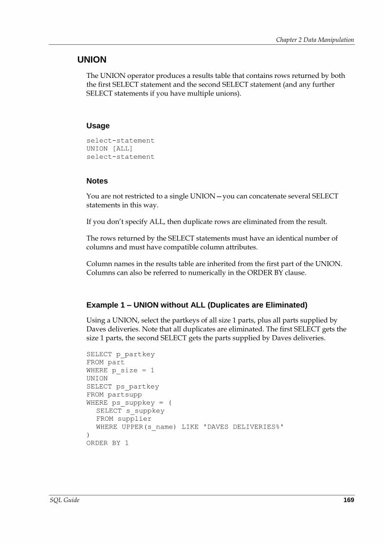
Chapter 2 Data Manipulation
SQL Guide 169
UNION
The UNION operator produces a results table that contains rows returned by both the first SELECT statement and the second SELECT statement (and any further SELECT statements if you have multiple unions).
Usage
select-statement
UNION [ALL]
select-statement
Notes
You are not restricted to a single UNION—you can concatenate several SELECT statements in this way.
If you don’t specify ALL, then duplicate rows are eliminated from the result.
The rows returned by the SELECT statements must have an identical number of columns and must have compatible column attributes.
Column names in the results table are inherited from the first part of the UNION. Columns can also be referred to numerically in the ORDER BY clause.
Example 1 – UNION without ALL (Duplicates are Eliminated)
Using a UNION, select the partkeys of all size 1 parts, plus all parts supplied by Daves deliveries. Note that all duplicates are eliminated. The first SELECT gets the size 1 parts, the second SELECT gets the parts supplied by Daves deliveries.
SELECT p_partkey
FROM part
WHERE p_size = 1
UNION
SELECT ps_partkey
FROM partsupp
WHERE ps_suppkey = (
SELECT s_suppkey
FROM supplier
WHERE UPPER(s_name) LIKE 'DAVES DELIVERIES%'
)
ORDER BY 1
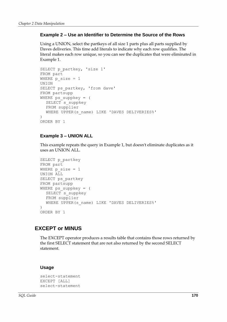
Chapter 2 Data Manipulation
SQL Guide 170
Example 2 – Use an Identifier to Determine the Source of the Rows
Using a UNION, select the partkeys of all size 1 parts plus all parts supplied by Daves deliveries. This time add literals to indicate why each row qualifies. The literal makes each row unique, so you can see the duplicates that were eliminated in Example 1.
SELECT p_partkey, 'size 1'
FROM part
WHERE p_size = 1
UNION
SELECT ps_partkey, 'from dave'
FROM partsupp
WHERE ps_suppkey = (
SELECT s_suppkey
FROM supplier
WHERE UPPER(s_name) LIKE 'DAVES DELIVERIES%'
)
ORDER BY 1
Example 3 – UNION ALL
This example repeats the query in Example 1, but doesn't eliminate duplicates as it uses an UNION ALL.
SELECT p_partkey
FROM part
WHERE p_size = 1
UNION ALL
SELECT ps_partkey
FROM partsupp
WHERE ps_suppkey = (
SELECT s_suppkey
FROM supplier
WHERE UPPER(s_name) LIKE 'DAVES DELIVERIES%'
)
ORDER BY 1
EXCEPT or MINUS
The EXCEPT operator produces a results table that contains those rows returned by the first SELECT statement that are not also returned by the second SELECT statement.
Usage
select-statement
EXCEPT [ALL]
select-statement
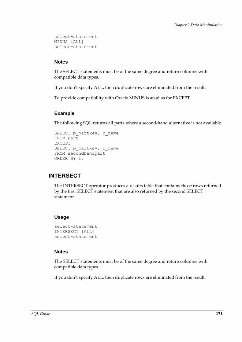
Chapter 2 Data Manipulation
SQL Guide 171
select-statement
MINUS [ALL]
select-statement
Notes
The SELECT statements must be of the same degree and return columns with compatible data types.
If you don’t specify ALL, then duplicate rows are eliminated from the result.
To provide compatibility with Oracle MINUS is an alias for EXCEPT.
Example
The following SQL returns all parts where a second-hand alternative is not available.
SELECT p_partkey, p_name
FROM part
EXCEPT
SELECT p_partkey, p_name
FROM secondhandpart
ORDER BY 1;
INTERSECT
The INTERSECT operator produces a results table that contains those rows returned by the first SELECT statement that are also returned by the second SELECT statement.
Usage
select-statement
INTERSECT [ALL]
select-statement
Notes
The SELECT statements must be of the same degree and return columns with compatible data types.
If you don’t specify ALL, then duplicate rows are eliminated from the result.
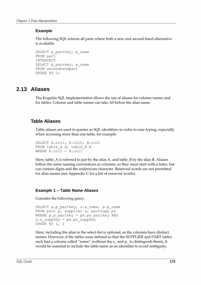
Chapter 2 Data Manipulation
SQL Guide 172
Example
The following SQL returns all parts where both a new and second-hand alternative is available.
SELECT p_partkey, p_name
FROM part
INTERSECT
SELECT p_partkey, p_name
FROM secondhandpart
ORDER BY 1;
2.13 Aliases
The Kognitio SQL implementation allows the use of aliases for column names and for tables. Column and table names can take AS before the alias name.
Table Aliases
Table aliases are used in queries as SQL identifiers in order to ease typing, especially when accessing more than one table, for example
SELECT A.col1, A.col2, B.col1
FROM table_A A, table_B B
WHERE A.col1 = B.col1
Here, table_A is referred to just by the alias A, and table_B by the alias B. Aliases follow the same naming conventions as columns, so they must start with a letter, but can contain digits and the underscore character. Reserved words are not permitted for alias names (see Appendix C for a list of reserved words).
Example 1 – Table Name Aliases
Consider the following query.
SELECT p.p_partkey, s.s_name, p.p_name
FROM part p, supplier s, partsupp ps
WHERE p.p_partkey = ps.ps_partkey AND
s.s_suppkey = ps.ps_suppkey
ORDER BY 1, 2
Here, including the alias in the select-list is optional, as the columns have distinct names. However, if the tables were defined so that the SUPPLIER and PART tables each had a column called “name” (without the s_ and p_ to distinguish them), it would be essential to include the table name as an identifier to avoid ambiguity.
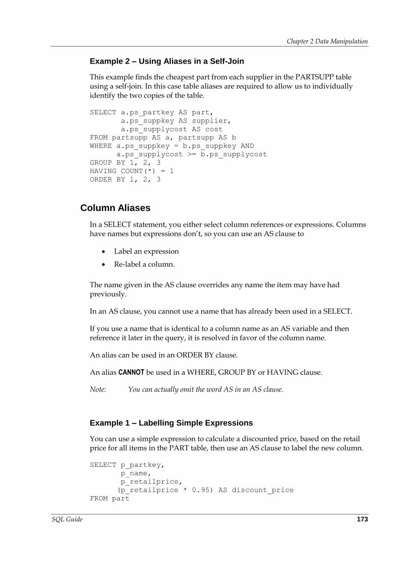
Chapter 2 Data Manipulation
SQL Guide 173
Example 2 – Using Aliases in a Self-Join
This example finds the cheapest part from each supplier in the PARTSUPP table using a self-join. In this case table aliases are required to allow us to individually identify the two copies of the table.
SELECT a.ps_partkey AS part,
a.ps_suppkey AS supplier,
a.ps_supplycost AS cost
FROM partsupp AS a, partsupp AS b
WHERE a.ps_suppkey = b.ps_suppkey AND
a.ps_supplycost >= b.ps_supplycost
GROUP BY 1, 2, 3
HAVING COUNT(*) = 1
ORDER BY 1, 2, 3
Column Aliases
In a SELECT statement, you either select column references or expressions. Columns have names but expressions don’t, so you can use an AS clause to
Label an expression
Re-label a column.
The name given in the AS clause overrides any name the item may have had previously.
In an AS clause, you cannot use a name that has already been used in a SELECT.
If you use a name that is identical to a column name as an AS variable and then reference it later in the query, it is resolved in favor of the column name.
An alias can be used in an ORDER BY clause.
An alias CANNOT be used in a WHERE, GROUP BY or HAVING clause.
Note: You can actually omit the word AS in an AS clause.
Example 1 – Labelling Simple Expressions
You can use a simple expression to calculate a discounted price, based on the retail price for all items in the PART table, then use an AS clause to label the new column.
SELECT p_partkey,
p_name,
p_retailprice,
(p_retailprice * 0.95) AS discount_price
FROM part
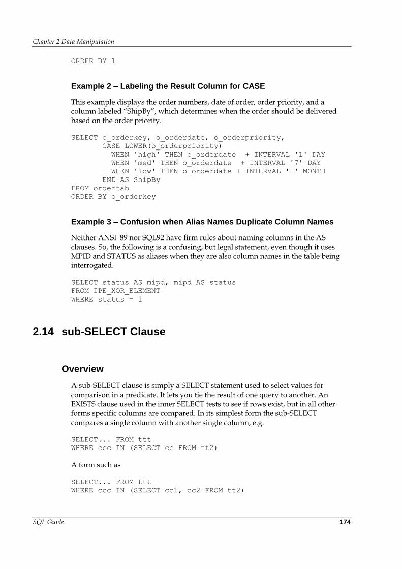
Chapter 2 Data Manipulation
SQL Guide 174
ORDER BY 1
Example 2 – Labeling the Result Column for CASE
This example displays the order numbers, date of order, order priority, and a column labeled “ShipBy”, which determines when the order should be delivered based on the order priority.
SELECT o_orderkey, o_orderdate, o_orderpriority,
CASE LOWER(o_orderpriority)
WHEN 'high' THEN o_orderdate + INTERVAL '1' DAY
WHEN 'med' THEN o_orderdate + INTERVAL '7' DAY
WHEN 'low' THEN o_orderdate + INTERVAL '1' MONTH
END AS ShipBy
FROM ordertab
ORDER BY o_orderkey
Example 3 – Confusion when Alias Names Duplicate Column Names
Neither ANSI '89 nor SQL92 have firm rules about naming columns in the AS clauses. So, the following is a confusing, but legal statement, even though it uses MPID and STATUS as aliases when they are also column names in the table being interrogated.
SELECT status AS mipd, mipd AS status
FROM IPE_XOR_ELEMENT
WHERE status = 1
2.14 sub-SELECT Clause
Overview
A sub-SELECT clause is simply a SELECT statement used to select values for comparison in a predicate. It lets you tie the result of one query to another. An EXISTS clause used in the inner SELECT tests to see if rows exist, but in all other forms specific columns are compared. In its simplest form the sub-SELECT compares a single column with another single column, e.g.
SELECT... FROM ttt
WHERE ccc IN (SELECT cc FROM tt2)
A form such as
SELECT... FROM ttt
WHERE ccc IN (SELECT cc1, cc2 FROM tt2)
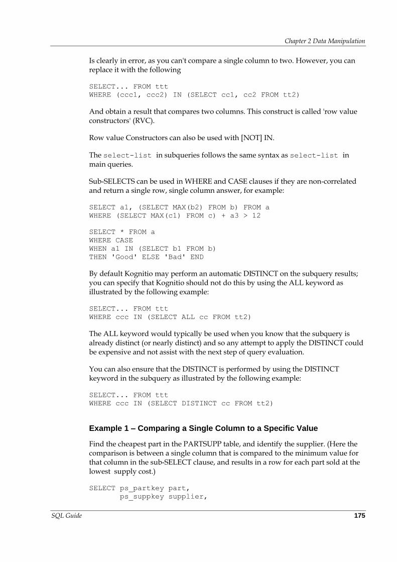
Chapter 2 Data Manipulation
SQL Guide 175
Is clearly in error, as you can't compare a single column to two. However, you can replace it with the following
SELECT... FROM ttt
WHERE (ccc1, ccc2) IN (SELECT cc1, cc2 FROM tt2)
And obtain a result that compares two columns. This construct is called 'row value constructors' (RVC).
Row value Constructors can also be used with [NOT] IN.
The select-list in subqueries follows the same syntax as select-list in main queries.
Sub-SELECTS can be used in WHERE and CASE clauses if they are non-correlated and return a single row, single column answer, for example:
SELECT a1, (SELECT MAX(b2) FROM b) FROM a
WHERE (SELECT MAX(c1) FROM c) + a3 > 12
SELECT * FROM a
WHERE CASE
WHEN a1 IN (SELECT b1 FROM b)
THEN 'Good' ELSE 'Bad' END
By default Kognitio may perform an automatic DISTINCT on the subquery results; you can specify that Kognitio should not do this by using the ALL keyword as illustrated by the following example:
SELECT... FROM ttt
WHERE ccc IN (SELECT ALL cc FROM tt2)
The ALL keyword would typically be used when you know that the subquery is already distinct (or nearly distinct) and so any attempt to apply the DISTINCT could be expensive and not assist with the next step of query evaluation.
You can also ensure that the DISTINCT is performed by using the DISTINCT keyword in the subquery as illustrated by the following example:
SELECT... FROM ttt
WHERE ccc IN (SELECT DISTINCT cc FROM tt2)
Example 1 – Comparing a Single Column to a Specific Value
Find the cheapest part in the PARTSUPP table, and identify the supplier. (Here the comparison is between a single column that is compared to the minimum value for that column in the sub-SELECT clause, and results in a row for each part sold at the lowest supply cost.)
SELECT ps_partkey part,
ps_suppkey supplier,
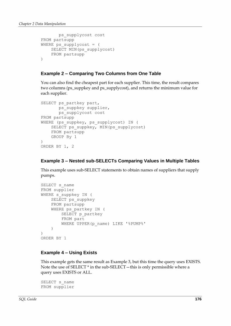
Chapter 2 Data Manipulation
SQL Guide 176
ps_supplycost cost
FROM partsupp
WHERE ps_supplycost = (
SELECT MIN(ps_supplycost)
FROM partsupp
)
Example 2 – Comparing Two Columns from One Table
You can also find the cheapest part for each supplier. This time, the result compares two columns (ps_suppkey and ps_supplycost), and returns the minimum value for each supplier.
SELECT ps_partkey part,
ps_suppkey supplier,
ps_supplycost cost
FROM partsupp
WHERE (ps_suppkey, ps_supplycost) IN (
SELECT ps_suppkey, MIN(ps_supplycost)
FROM partsupp
GROUP By 1
)
ORDER BY 1, 2
Example 3 – Nested sub-SELECTs Comparing Values in Multiple Tables
This example uses sub-SELECT statements to obtain names of suppliers that supply pumps.
SELECT s_name
FROM supplier
WHERE s_suppkey IN (
SELECT ps_suppkey
FROM partsupp
WHERE ps_partkey IN (
SELECT p_partkey
FROM part
WHERE UPPER(p_name) LIKE '%PUMP%'
)
)
ORDER BY 1
Example 4 – Using Exists
This example gets the same result as Example 3, but this time the query uses EXISTS. Note the use of SELECT * in the sub-SELECT—this is only permissible where a query uses EXISTS or ALL.
SELECT s_name
FROM supplier
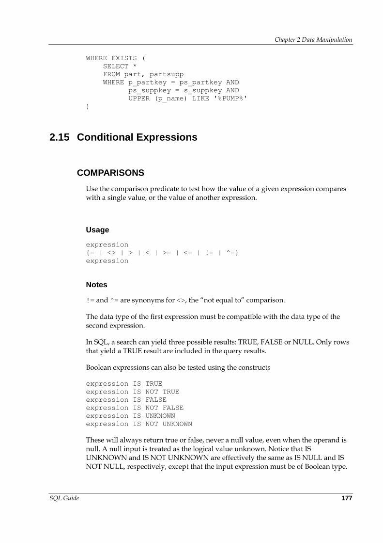
Chapter 2 Data Manipulation
SQL Guide 177
WHERE EXISTS (
SELECT *
FROM part, partsupp
WHERE p_partkey = ps_partkey AND
ps_suppkey = s_suppkey AND
UPPER (p_name) LIKE '%PUMP%'
)
2.15 Conditional Expressions
COMPARISONS
Use the comparison predicate to test how the value of a given expression compares with a single value, or the value of another expression.
Usage
expression
{= | <> | > | < | >= | <= | != | ^=}
expression
Notes
!= and ^= are synonyms for <>, the “not equal to” comparison.
The data type of the first expression must be compatible with the data type of the second expression.
In SQL, a search can yield three possible results: TRUE, FALSE or NULL. Only rows that yield a TRUE result are included in the query results.
Boolean expressions can also be tested using the constructs
expression IS TRUE
expression IS NOT TRUE
expression IS FALSE
expression IS NOT FALSE
expression IS UNKNOWN
expression IS NOT UNKNOWN
These will always return true or false, never a null value, even when the operand is null. A null input is treated as the logical value unknown. Notice that IS UNKNOWN and IS NOT UNKNOWN are effectively the same as IS NULL and IS NOT NULL, respectively, except that the input expression must be of Boolean type.
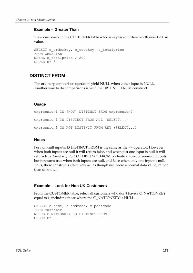
Chapter 2 Data Manipulation
SQL Guide 178
Example – Greater Than
View customers in the CUSTOMER table who have placed orders worth over £200 in value.
SELECT o_orderkey, o_custkey, o_totalprice
FROM ORDERTAB
WHERE o_totalprice > 200
ORDER BY 3
DISTINCT FROM
The ordinary comparison operators yield NULL when either input is NULL. Another way to do comparisons is with the DISTINCT FROM construct.
Usage
expression1 IS [NOT] DISTINCT FROM expression2
expression1 IS DISTINCT FROM ALL (SELECT...)
expression1 IS NOT DISTINCT FROM ANY (SELECT...)
Notes
For non-null inputs, IS DISTINCT FROM is the same as the <> operator. However, when both inputs are null it will return false, and when just one input is null it will return true. Similarly, IS NOT DISTINCT FROM is identical to = for non-null inputs, but it returns true when both inputs are null, and false when only one input is null. Thus, these constructs effectively act as though null were a normal data value, rather than unknown.
Example – Look for Non UK Customers
From the CUSTOMER table, select all customers who don't have a C_NATIONKEY equal to 1, including those where the C_NATIONKEY is NULL.
SELECT c_name, c_address, c_postcode
FROM customer
WHERE C_NATIONKEY IS DISTINCT FROM 1
ORDER BY 3
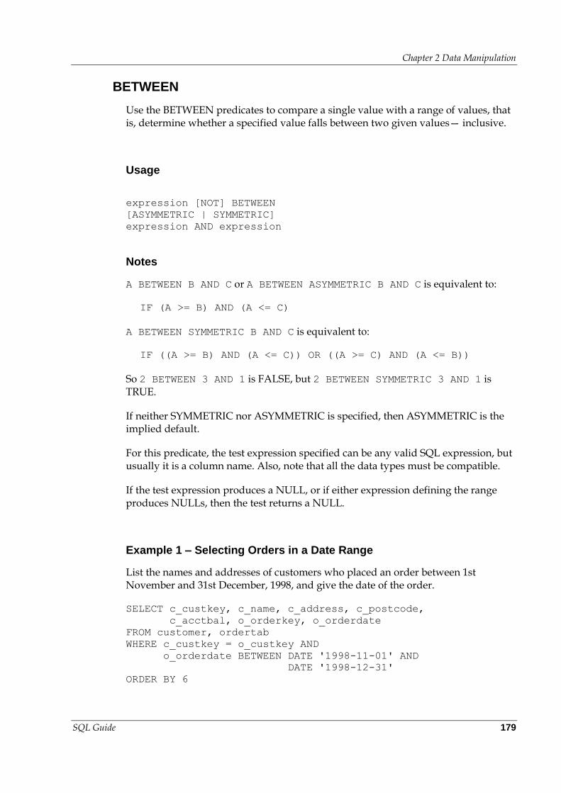
Chapter 2 Data Manipulation
SQL Guide 179
BETWEEN
Use the BETWEEN predicates to compare a single value with a range of values, that is, determine whether a specified value falls between two given values— inclusive.
Usage
expression [NOT] BETWEEN
[ASYMMETRIC | SYMMETRIC]
expression AND expression
Notes
A BETWEEN B AND C or A BETWEEN ASYMMETRIC B AND C is equivalent to:
IF (A >= B) AND (A <= C)
A BETWEEN SYMMETRIC B AND C is equivalent to:
IF ((A >= B) AND (A <= C)) OR ((A >= C) AND (A <= B))
So 2 BETWEEN 3 AND 1 is FALSE, but 2 BETWEEN SYMMETRIC 3 AND 1 is TRUE.
If neither SYMMETRIC nor ASYMMETRIC is specified, then ASYMMETRIC is the implied default.
For this predicate, the test expression specified can be any valid SQL expression, but usually it is a column name. Also, note that all the data types must be compatible.
If the test expression produces a NULL, or if either expression defining the range produces NULLs, then the test returns a NULL.
Example 1 – Selecting Orders in a Date Range
List the names and addresses of customers who placed an order between 1st November and 31st December, 1998, and give the date of the order.
SELECT c_custkey, c_name, c_address, c_postcode,
c_acctbal, o_orderkey, o_orderdate
FROM customer, ordertab
WHERE c_custkey = o_custkey AND
o_orderdate BETWEEN DATE '1998-11-01' AND
DATE '1998-12-31'
ORDER BY 6
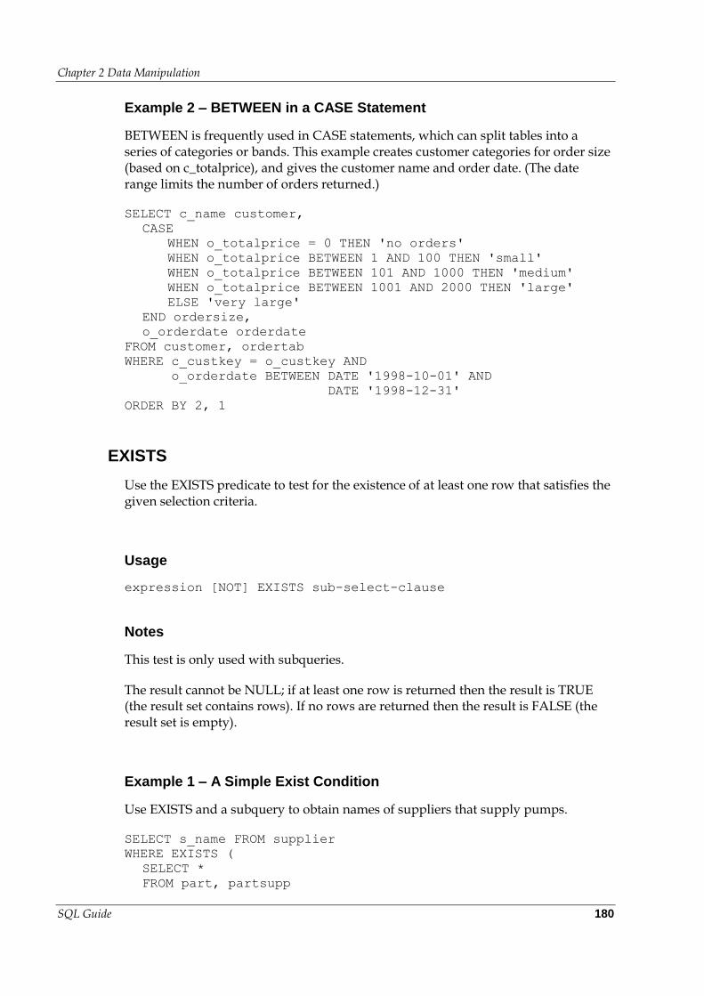
Chapter 2 Data Manipulation
SQL Guide 180
Example 2 – BETWEEN in a CASE Statement
BETWEEN is frequently used in CASE statements, which can split tables into a series of categories or bands. This example creates customer categories for order size (based on c_totalprice), and gives the customer name and order date. (The date range limits the number of orders returned.)
SELECT c_name customer,
CASE
WHEN o_totalprice = 0 THEN 'no orders'
WHEN o_totalprice BETWEEN 1 AND 100 THEN 'small'
WHEN o_totalprice BETWEEN 101 AND 1000 THEN 'medium'
WHEN o_totalprice BETWEEN 1001 AND 2000 THEN 'large'
ELSE 'very large'
END ordersize,
o_orderdate orderdate
FROM customer, ordertab
WHERE c_custkey = o_custkey AND
o_orderdate BETWEEN DATE '1998-10-01' AND
DATE '1998-12-31'
ORDER BY 2, 1
EXISTS
Use the EXISTS predicate to test for the existence of at least one row that satisfies the given selection criteria.
Usage
expression [NOT] EXISTS sub-select-clause
Notes
This test is only used with subqueries.
The result cannot be NULL; if at least one row is returned then the result is TRUE (the result set contains rows). If no rows are returned then the result is FALSE (the result set is empty).
Example 1 – A Simple Exist Condition
Use EXISTS and a subquery to obtain names of suppliers that supply pumps.
SELECT s_name FROM supplier
WHERE EXISTS (
SELECT *
FROM part, partsupp
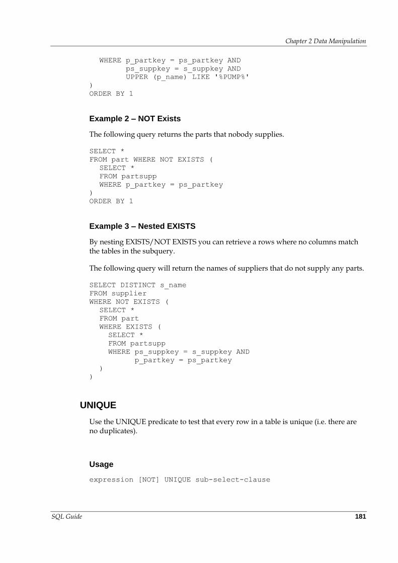
Chapter 2 Data Manipulation
SQL Guide 181
WHERE p_partkey = ps_partkey AND
ps_suppkey = s_suppkey AND
UPPER (p_name) LIKE '%PUMP%'
)
ORDER BY 1
Example 2 – NOT Exists
The following query returns the parts that nobody supplies.
SELECT *
FROM part WHERE NOT EXISTS (
SELECT *
FROM partsupp
WHERE p_partkey = ps_partkey
)
ORDER BY 1
Example 3 – Nested EXISTS
By nesting EXISTS/NOT EXISTS you can retrieve a rows where no columns match the tables in the subquery.
The following query will return the names of suppliers that do not supply any parts.
SELECT DISTINCT s_name
FROM supplier
WHERE NOT EXISTS (
SELECT *
FROM part
WHERE EXISTS (
SELECT *
FROM partsupp
WHERE ps_suppkey = s_suppkey AND
p_partkey = ps_partkey
)
)
UNIQUE
Use the UNIQUE predicate to test that every row in a table is unique (i.e. there are no duplicates).
Usage
expression [NOT] UNIQUE sub-select-clause
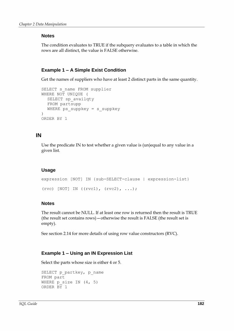
Chapter 2 Data Manipulation
SQL Guide 182
Notes
The condition evaluates to TRUE if the subquery evaluates to a table in which the rows are all distinct, the value is FALSE otherwise.
Example 1 – A Simple Exist Condition
Get the names of suppliers who have at least 2 distinct parts in the same quantity.
SELECT s_name FROM supplier
WHERE NOT UNIQUE (
SELECT sp_availqty
FROM partsupp
WHERE ps_suppkey = s_suppkey
)
ORDER BY 1
IN
Use the predicate IN to test whether a given value is (un)equal to any value in a given list.
Usage
expression [NOT] IN {sub-SELECT-clause | expression-list}
(rvc) [NOT] IN ((rvc1), (rvc2), ...);
Notes
The result cannot be NULL. If at least one row is returned then the result is TRUE (the result set contains rows)—otherwise the result is FALSE (the result set is empty).
See section 2.14 for more details of using row value constructors (RVC).
Example 1 – Using an IN Expression List
Select the parts whose size is either 4 or 5.
SELECT p_partkey, p_name
FROM part
WHERE p_size IN (4, 5)
ORDER BY 1
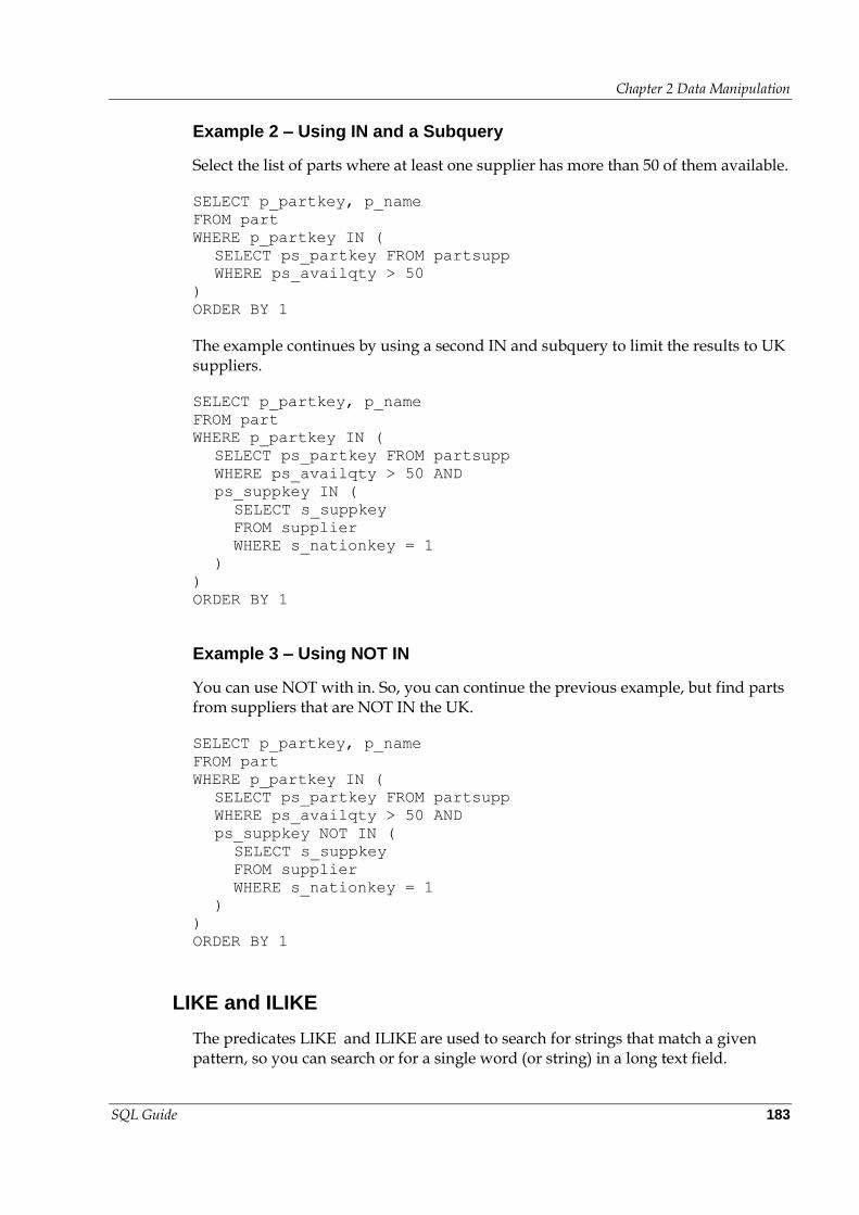
Chapter 2 Data Manipulation
SQL Guide 183
Example 2 – Using IN and a Subquery
Select the list of parts where at least one supplier has more than 50 of them available.
SELECT p_partkey, p_name
FROM part
WHERE p_partkey IN (
SELECT ps_partkey FROM partsupp
WHERE ps_availqty > 50
)
ORDER BY 1
The example continues by using a second IN and subquery to limit the results to UK suppliers.
SELECT p_partkey, p_name
FROM part
WHERE p_partkey IN (
SELECT ps_partkey FROM partsupp
WHERE ps_availqty > 50 AND
ps_suppkey IN (
SELECT s_suppkey
FROM supplier
WHERE s_nationkey = 1
)
)
ORDER BY 1
Example 3 – Using NOT IN
You can use NOT with in. So, you can continue the previous example, but find parts from suppliers that are NOT IN the UK.
SELECT p_partkey, p_name
FROM part
WHERE p_partkey IN (
SELECT ps_partkey FROM partsupp
WHERE ps_availqty > 50 AND
ps_suppkey NOT IN (
SELECT s_suppkey
FROM supplier
WHERE s_nationkey = 1
)
)
ORDER BY 1
LIKE and ILIKE
The predicates LIKE and ILIKE are used to search for strings that match a given pattern, so you can search or for a single word (or string) in a long text field.
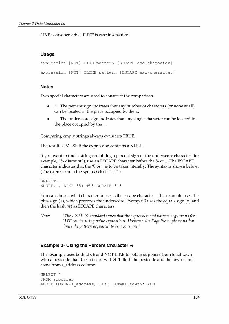
Chapter 2 Data Manipulation
SQL Guide 184
LIKE is case sensitive, ILIKE is case insensitive.
Usage
expression [NOT] LIKE pattern [ESCAPE esc-character]
expression [NOT] ILIKE pattern [ESCAPE esc-character]
Notes
Two special characters are used to construct the comparison.
% The percent sign indicates that any number of characters (or none at all) can be located in the place occupied by the %.
_ The underscore sign indicates that any single character can be located in the place occupied by the _.
Comparing empty strings always evaluates TRUE.
The result is FALSE if the expression contains a NULL.
If you want to find a string containing a percent sign or the underscore character (for example, “% discount”), use an ESCAPE character before the % or _. The ESCAPE character indicates that the % or _ is to be taken literally. The syntax is shown below. (The expression in the syntax selects “_T”.)
SELECT...
WHERE... LIKE '%+_T%' ESCAPE '+'
You can choose what character to use as the escape character—this example uses the plus sign (+), which precedes the underscore. Example 3 uses the equals sign (=) and then the hash (#) as ESCAPE characters.
Note: "The ANSI '92 standard states that the expression and pattern arguments for LIKE can be string value expressions. However, the Kognitio implementation limits the pattern argument to be a constant."
Example 1- Using the Percent Character %
This example uses both LIKE and NOT LIKE to obtain suppliers from Smalltown with a postcode that doesn’t start with ST1. Both the postcode and the town name come from s_address column.
SELECT *
FROM supplier
WHERE LOWER(s_address) LIKE '%smalltown%' AND
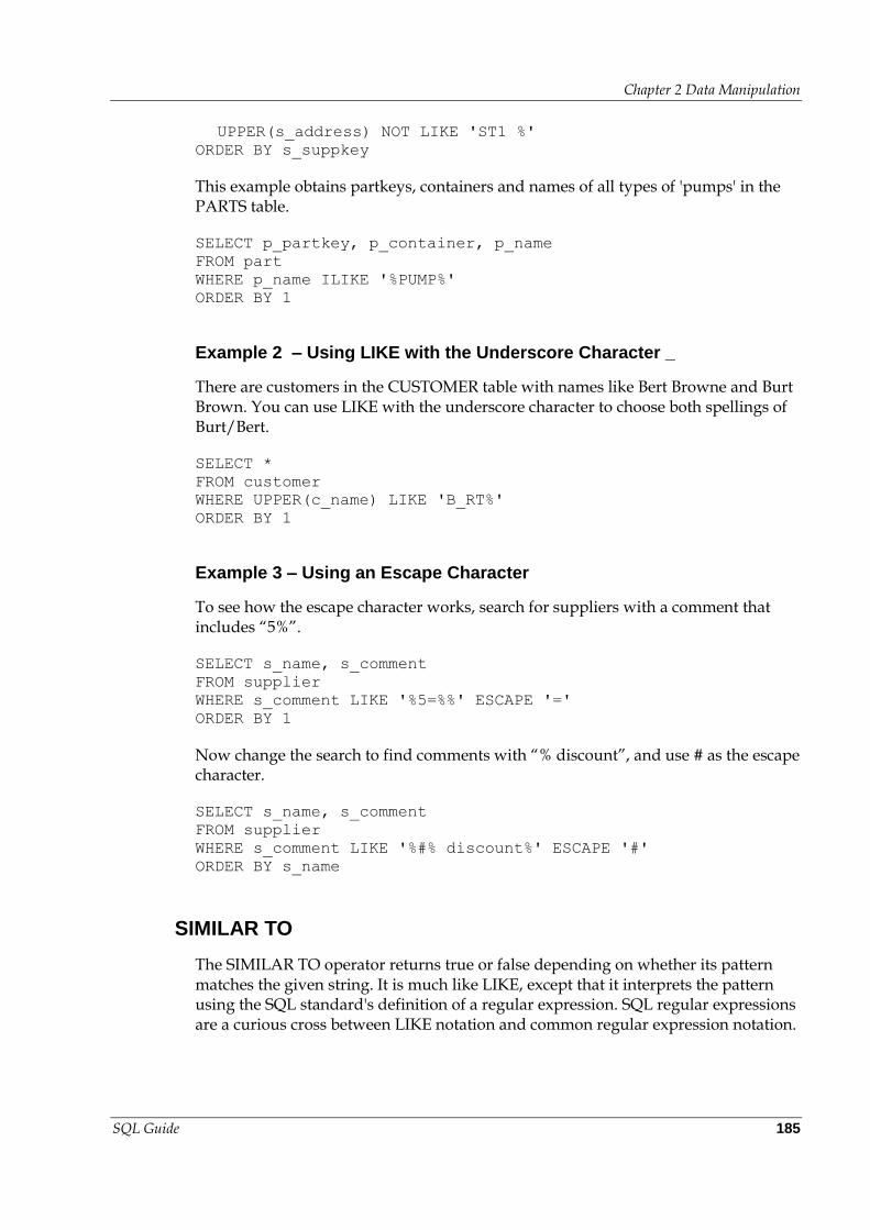
Chapter 2 Data Manipulation
SQL Guide 185
UPPER(s_address) NOT LIKE 'ST1 %'
ORDER BY s_suppkey
This example obtains partkeys, containers and names of all types of 'pumps' in the PARTS table.
SELECT p_partkey, p_container, p_name
FROM part
WHERE p_name ILIKE '%PUMP%'
ORDER BY 1
Example 2 – Using LIKE with the Underscore Character _
There are customers in the CUSTOMER table with names like Bert Browne and Burt Brown. You can use LIKE with the underscore character to choose both spellings of Burt/Bert.
SELECT *
FROM customer
WHERE UPPER(c_name) LIKE 'B_RT%'
ORDER BY 1
Example 3 – Using an Escape Character
To see how the escape character works, search for suppliers with a comment that includes “5%”.
SELECT s_name, s_comment
FROM supplier
WHERE s_comment LIKE '%5=%%' ESCAPE '='
ORDER BY 1
Now change the search to find comments with “% discount”, and use # as the escape character.
SELECT s_name, s_comment
FROM supplier
WHERE s_comment LIKE '%#% discount%' ESCAPE '#'
ORDER BY s_name
SIMILAR TO
The SIMILAR TO operator returns true or false depending on whether its pattern matches the given string. It is much like LIKE, except that it interprets the pattern using the SQL standard's definition of a regular expression. SQL regular expressions are a curious cross between LIKE notation and common regular expression notation.
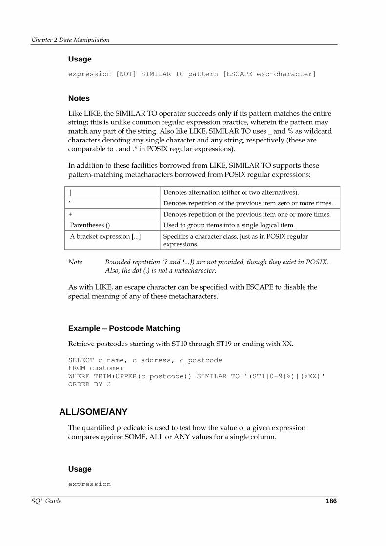
Chapter 2 Data Manipulation
SQL Guide 186
Usage
expression [NOT] SIMILAR TO pattern [ESCAPE esc-character]
Notes
Like LIKE, the SIMILAR TO operator succeeds only if its pattern matches the entire string; this is unlike common regular expression practice, wherein the pattern may match any part of the string. Also like LIKE, SIMILAR TO uses _ and % as wildcard characters denoting any single character and any string, respectively (these are comparable to . and .* in POSIX regular expressions).
In addition to these facilities borrowed from LIKE, SIMILAR TO supports these pattern-matching metacharacters borrowed from POSIX regular expressions:
| Denotes alternation (either of two alternatives).
* Denotes repetition of the previous item zero or more times.
+ Denotes repetition of the previous item one or more times.
Parentheses () Used to group items into a single logical item.
A bracket expression [...] Specifies a character class, just as in POSIX regular expressions.
Note Bounded repetition (? and {...}) are not provided, though they exist in POSIX. Also, the dot (.) is not a metacharacter.
As with LIKE, an escape character can be specified with ESCAPE to disable the special meaning of any of these metacharacters.
Example – Postcode Matching
Retrieve postcodes starting with ST10 through ST19 or ending with XX.
SELECT c_name, c_address, c_postcode
FROM customer
WHERE TRIM(UPPER(c_postcode)) SIMILAR TO '(ST1[0-9]%)|(%XX)'
ORDER BY 3
ALL/SOME/ANY
The quantified predicate is used to test how the value of a given expression compares against SOME, ALL or ANY values for a single column.
Usage
expression
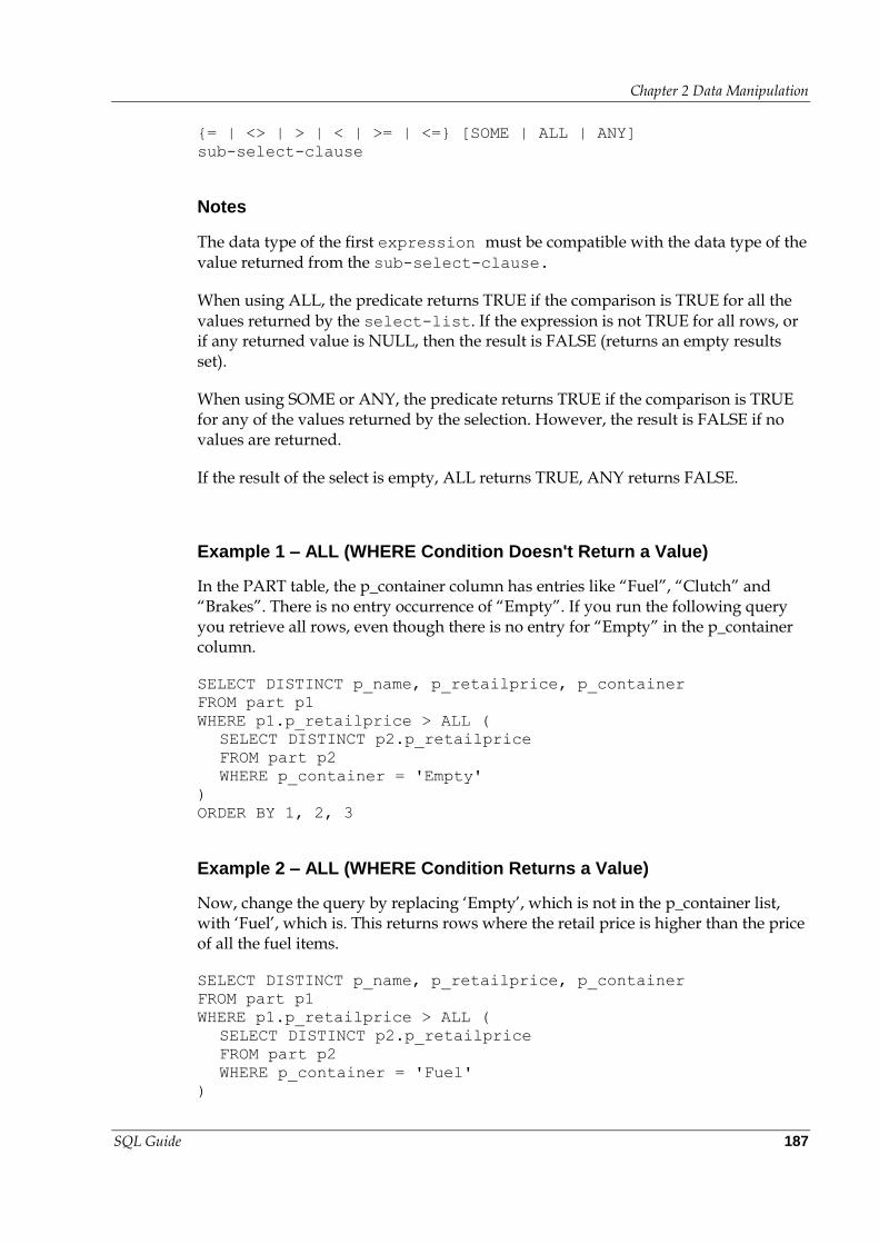
Chapter 2 Data Manipulation
SQL Guide 187
{= | <> | > | < | >= | <=} [SOME | ALL | ANY]
sub-select-clause
Notes
The data type of the first expression must be compatible with the data type of the value returned from the sub-select-clause.
When using ALL, the predicate returns TRUE if the comparison is TRUE for all the values returned by the select-list. If the expression is not TRUE for all rows, or if any returned value is NULL, then the result is FALSE (returns an empty results set).
When using SOME or ANY, the predicate returns TRUE if the comparison is TRUE for any of the values returned by the selection. However, the result is FALSE if no values are returned.
If the result of the select is empty, ALL returns TRUE, ANY returns FALSE.
Example 1 – ALL (WHERE Condition Doesn't Return a Value)
In the PART table, the p_container column has entries like “Fuel”, “Clutch” and “Brakes”. There is no entry occurrence of “Empty”. If you run the following query you retrieve all rows, even though there is no entry for “Empty” in the p_container column.
SELECT DISTINCT p_name, p_retailprice, p_container
FROM part p1
WHERE p1.p_retailprice > ALL (
SELECT DISTINCT p2.p_retailprice
FROM part p2
WHERE p_container = 'Empty'
)
ORDER BY 1, 2, 3
Example 2 – ALL (WHERE Condition Returns a Value)
Now, change the query by replacing ‘Empty’, which is not in the p_container list, with ‘Fuel’, which is. This returns rows where the retail price is higher than the price of all the fuel items.
SELECT DISTINCT p_name, p_retailprice, p_container
FROM part p1
WHERE p1.p_retailprice > ALL (
SELECT DISTINCT p2.p_retailprice
FROM part p2
WHERE p_container = 'Fuel'
)
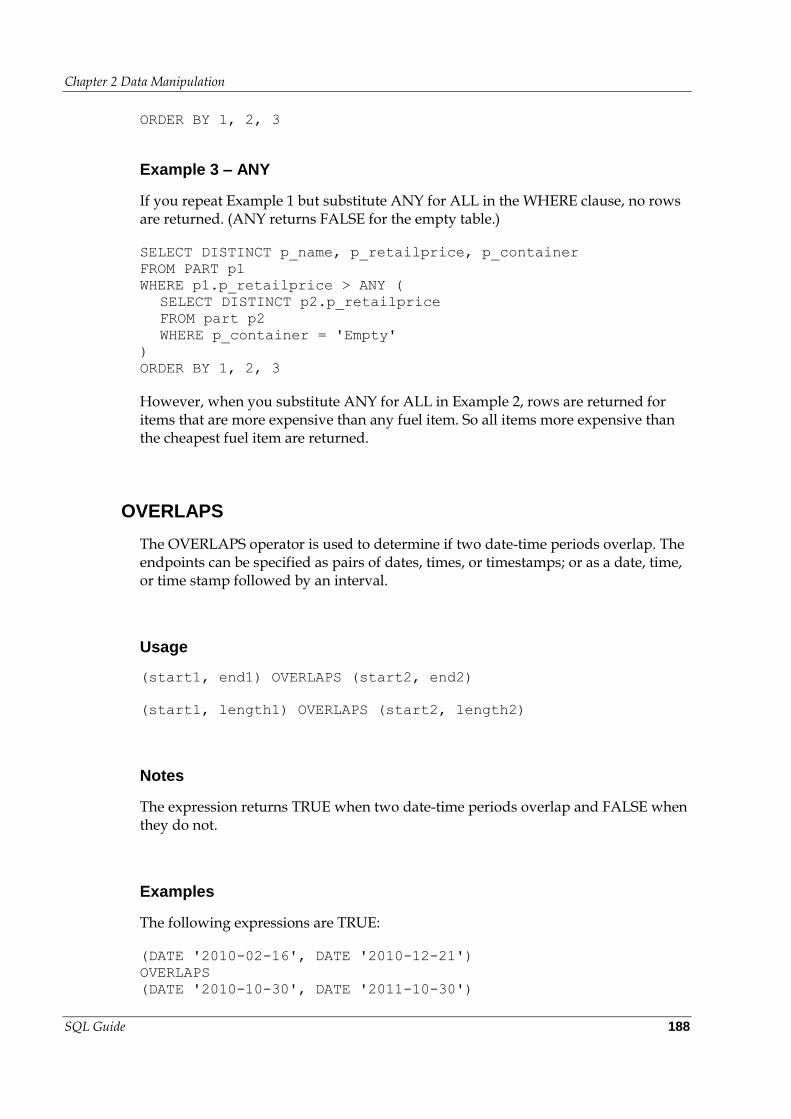
Chapter 2 Data Manipulation
SQL Guide 188
ORDER BY 1, 2, 3
Example 3 – ANY
If you repeat Example 1 but substitute ANY for ALL in the WHERE clause, no rows are returned. (ANY returns FALSE for the empty table.)
SELECT DISTINCT p_name, p_retailprice, p_container
FROM PART p1
WHERE p1.p_retailprice > ANY (
SELECT DISTINCT p2.p_retailprice
FROM part p2
WHERE p_container = 'Empty'
)
ORDER BY 1, 2, 3
However, when you substitute ANY for ALL in Example 2, rows are returned for items that are more expensive than any fuel item. So all items more expensive than the cheapest fuel item are returned.
OVERLAPS
The OVERLAPS operator is used to determine if two date-time periods overlap. The endpoints can be specified as pairs of dates, times, or timestamps; or as a date, time, or time stamp followed by an interval.
Usage
(start1, end1) OVERLAPS (start2, end2)
(start1, length1) OVERLAPS (start2, length2)
Notes
The expression returns TRUE when two date-time periods overlap and FALSE when they do not.
Examples
The following expressions are TRUE:
(DATE '2010-02-16', DATE '2010-12-21')
OVERLAPS
(DATE '2010-10-30', DATE '2011-10-30')
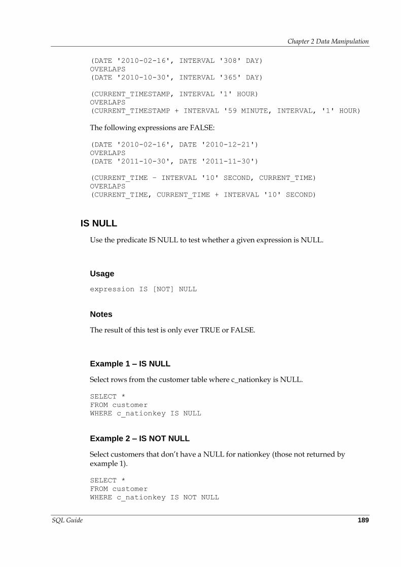
Chapter 2 Data Manipulation
SQL Guide 189
(DATE '2010-02-16', INTERVAL '308' DAY)
OVERLAPS
(DATE '2010-10-30', INTERVAL '365' DAY)
(CURRENT_TIMESTAMP, INTERVAL '1' HOUR)
OVERLAPS
(CURRENT_TIMESTAMP + INTERVAL '59 MINUTE, INTERVAL, '1' HOUR)
The following expressions are FALSE:
(DATE '2010-02-16', DATE '2010-12-21')
OVERLAPS
(DATE '2011-10-30', DATE '2011-11-30')
(CURRENT_TIME – INTERVAL '10' SECOND, CURRENT_TIME)
OVERLAPS
(CURRENT_TIME, CURRENT_TIME + INTERVAL '10' SECOND)
IS NULL
Use the predicate IS NULL to test whether a given expression is NULL.
Usage
expression IS [NOT] NULL
Notes
The result of this test is only ever TRUE or FALSE.
Example 1 – IS NULL
Select rows from the customer table where c_nationkey is NULL.
SELECT *
FROM customer
WHERE c_nationkey IS NULL
Example 2 – IS NOT NULL
Select customers that don’t have a NULL for nationkey (those not returned by example 1).
SELECT *
FROM customer
WHERE c_nationkey IS NOT NULL
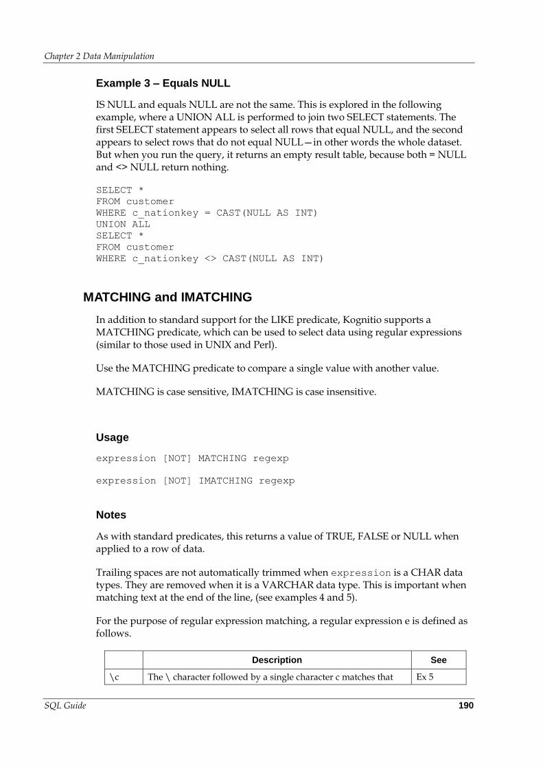
Chapter 2 Data Manipulation
SQL Guide 190
Example 3 – Equals NULL
IS NULL and equals NULL are not the same. This is explored in the following example, where a UNION ALL is performed to join two SELECT statements. The first SELECT statement appears to select all rows that equal NULL, and the second appears to select rows that do not equal NULL—in other words the whole dataset. But when you run the query, it returns an empty result table, because both = NULL and <> NULL return nothing.
SELECT *
FROM customer
WHERE c_nationkey = CAST(NULL AS INT)
UNION ALL
SELECT *
FROM customer
WHERE c_nationkey <> CAST(NULL AS INT)
MATCHING and IMATCHING
In addition to standard support for the LIKE predicate, Kognitio supports a MATCHING predicate, which can be used to select data using regular expressions (similar to those used in UNIX and Perl).
Use the MATCHING predicate to compare a single value with another value.
MATCHING is case sensitive, IMATCHING is case insensitive.
Usage
expression [NOT] MATCHING regexp
expression [NOT] IMATCHING regexp
Notes
As with standard predicates, this returns a value of TRUE, FALSE or NULL when applied to a row of data.
Trailing spaces are not automatically trimmed when expression is a CHAR data types. They are removed when it is a VARCHAR data type. This is important when matching text at the end of the line, (see examples 4 and 5).
For the purpose of regular expression matching, a regular expression e is defined as follows.
Description See
\c The \ character followed by a single character c matches that Ex 5
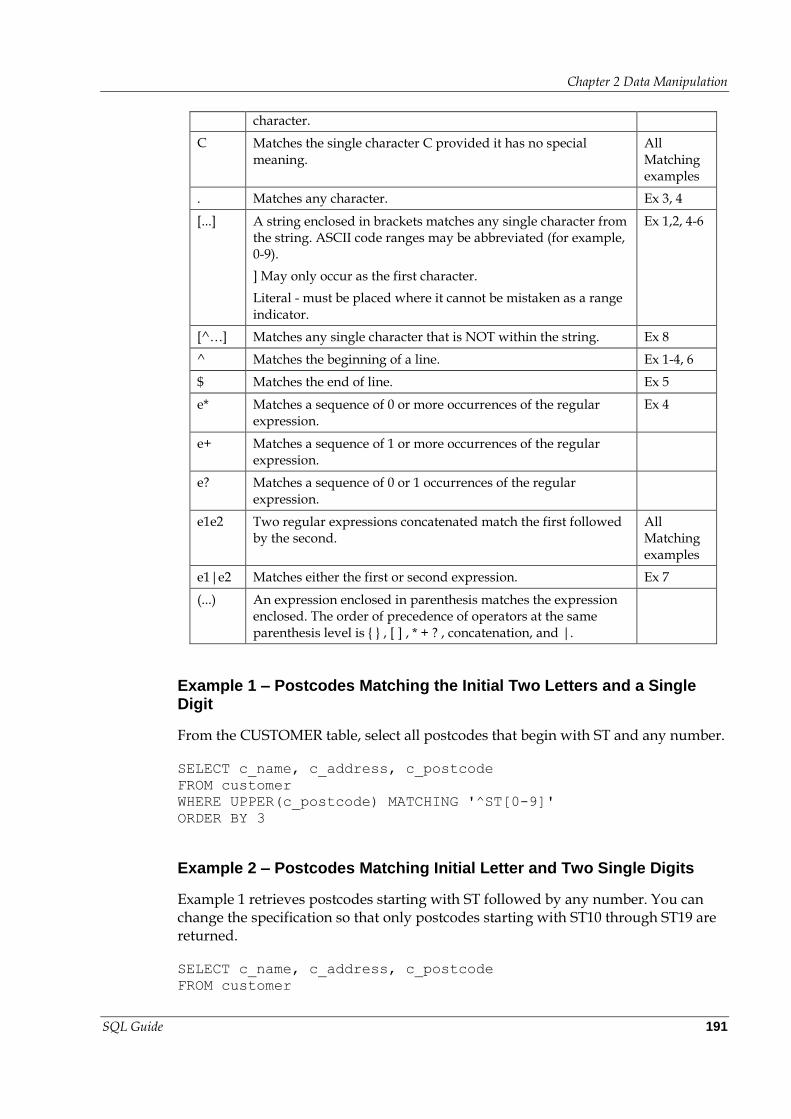
Chapter 2 Data Manipulation
SQL Guide 191
character.
C Matches the single character C provided it has no special meaning.
All Matching examples
. Matches any character. Ex 3, 4
[...] A string enclosed in brackets matches any single character from the string. ASCII code ranges may be abbreviated (for example, 0-9).
] May only occur as the first character.
Literal - must be placed where it cannot be mistaken as a range indicator.
Ex 1,2, 4-6
[^…] Matches any single character that is NOT within the string. Ex 8
^ Matches the beginning of a line. Ex 1-4, 6
$ Matches the end of line. Ex 5
e* Matches a sequence of 0 or more occurrences of the regular expression.
Ex 4
e+ Matches a sequence of 1 or more occurrences of the regular expression.
e? Matches a sequence of 0 or 1 occurrences of the regular expression.
e1e2 Two regular expressions concatenated match the first followed by the second.
All Matching examples
e1|e2 Matches either the first or second expression. Ex 7
(...) An expression enclosed in parenthesis matches the expression enclosed. The order of precedence of operators at the same parenthesis level is { } , [ ] , * + ? , concatenation, and |.
Example 1 – Postcodes Matching the Initial Two Letters and a Single Digit
From the CUSTOMER table, select all postcodes that begin with ST and any number.
SELECT c_name, c_address, c_postcode
FROM customer
WHERE UPPER(c_postcode) MATCHING '^ST[0-9]'
ORDER BY 3
Example 2 – Postcodes Matching Initial Letter and Two Single Digits
Example 1 retrieves postcodes starting with ST followed by any number. You can change the specification so that only postcodes starting with ST10 through ST19 are returned.
SELECT c_name, c_address, c_postcode
FROM customer
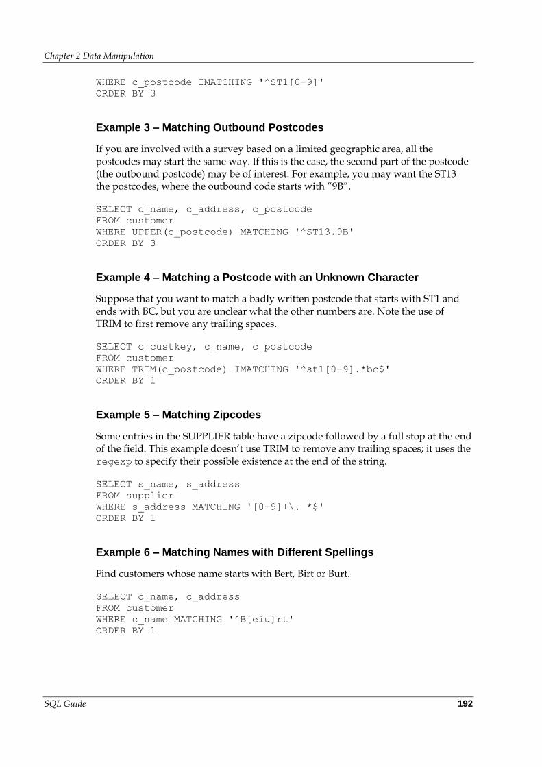
Chapter 2 Data Manipulation
SQL Guide 192
WHERE c_postcode IMATCHING '^ST1[0-9]'
ORDER BY 3
Example 3 – Matching Outbound Postcodes
If you are involved with a survey based on a limited geographic area, all the postcodes may start the same way. If this is the case, the second part of the postcode (the outbound postcode) may be of interest. For example, you may want the ST13 the postcodes, where the outbound code starts with “9B”.
SELECT c_name, c_address, c_postcode
FROM customer
WHERE UPPER(c_postcode) MATCHING '^ST13.9B'
ORDER BY 3
Example 4 – Matching a Postcode with an Unknown Character
Suppose that you want to match a badly written postcode that starts with ST1 and ends with BC, but you are unclear what the other numbers are. Note the use of TRIM to first remove any trailing spaces.
SELECT c_custkey, c_name, c_postcode
FROM customer
WHERE TRIM(c_postcode) IMATCHING '^st1[0-9].*bc$'
ORDER BY 1
Example 5 – Matching Zipcodes
Some entries in the SUPPLIER table have a zipcode followed by a full stop at the end of the field. This example doesn’t use TRIM to remove any trailing spaces; it uses the regexp to specify their possible existence at the end of the string.
SELECT s_name, s_address
FROM supplier
WHERE s_address MATCHING '[0-9]+\. *$'
ORDER BY 1
Example 6 – Matching Names with Different Spellings
Find customers whose name starts with Bert, Birt or Burt.
SELECT c_name, c_address
FROM customer
WHERE c_name MATCHING '^B[eiu]rt'
ORDER BY 1
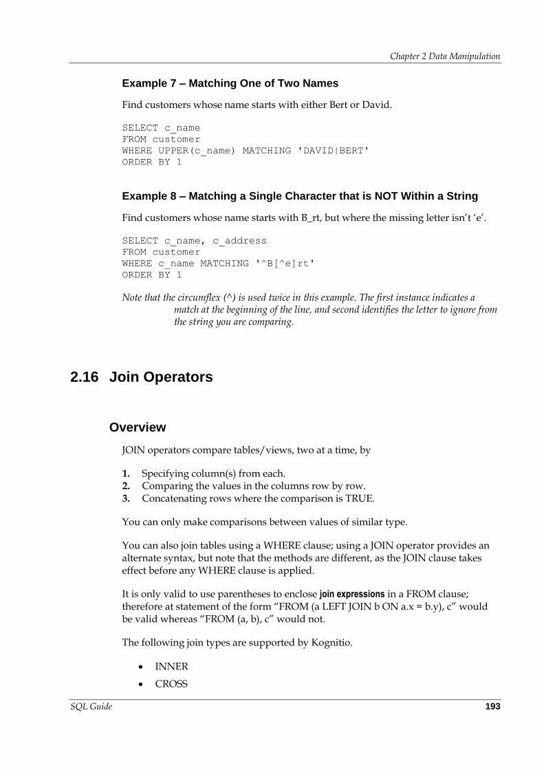
Chapter 2 Data Manipulation
SQL Guide 193
Example 7 – Matching One of Two Names
Find customers whose name starts with either Bert or David.
SELECT c_name
FROM customer
WHERE UPPER(c_name) MATCHING 'DAVID|BERT'
ORDER BY 1
Example 8 – Matching a Single Character that is NOT Within a String
Find customers whose name starts with B_rt, but where the missing letter isn’t ‘e’.
SELECT c_name, c_address
FROM customer
WHERE c_name MATCHING '^B[^e]rt'
ORDER BY 1
Note that the circumflex (^) is used twice in this example. The first instance indicates a match at the beginning of the line, and second identifies the letter to ignore from the string you are comparing.
2.16 Join Operators
Overview
JOIN operators compare tables/views, two at a time, by
1. Specifying column(s) from each. 2. Comparing the values in the columns row by row. 3. Concatenating rows where the comparison is TRUE.
You can only make comparisons between values of similar type.
You can also join tables using a WHERE clause; using a JOIN operator provides an alternate syntax, but note that the methods are different, as the JOIN clause takes effect before any WHERE clause is applied.
It is only valid to use parentheses to enclose join expressions in a FROM clause; therefore at statement of the form “FROM (a LEFT JOIN b ON a.x = b.y), c” would be valid whereas “FROM (a, b), c” would not.
The following join types are supported by Kognitio.
INNER
CROSS
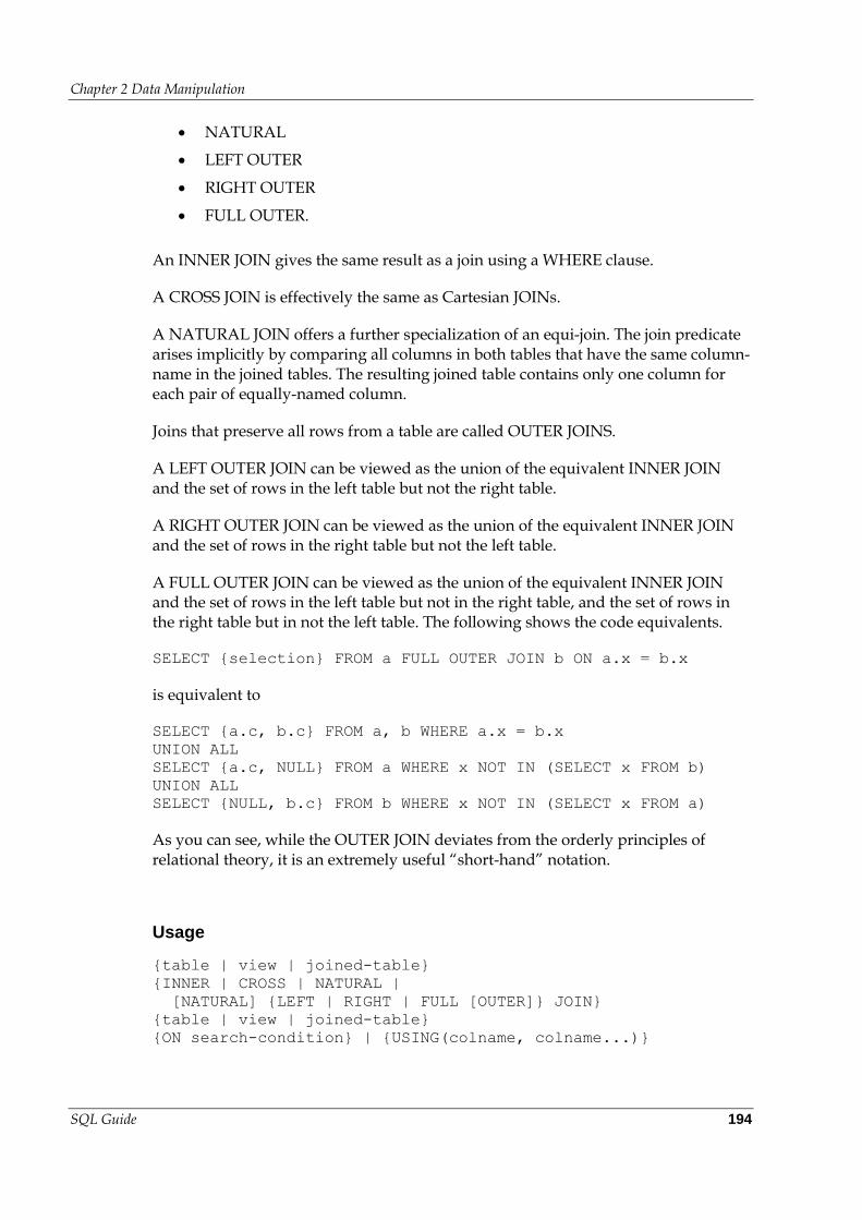
Chapter 2 Data Manipulation
SQL Guide 194
NATURAL
LEFT OUTER
RIGHT OUTER
FULL OUTER.
An INNER JOIN gives the same result as a join using a WHERE clause.
A CROSS JOIN is effectively the same as Cartesian JOINs.
A NATURAL JOIN offers a further specialization of an equi-join. The join predicate arises implicitly by comparing all columns in both tables that have the same column-name in the joined tables. The resulting joined table contains only one column for each pair of equally-named column.
Joins that preserve all rows from a table are called OUTER JOINS.
A LEFT OUTER JOIN can be viewed as the union of the equivalent INNER JOIN and the set of rows in the left table but not the right table.
A RIGHT OUTER JOIN can be viewed as the union of the equivalent INNER JOIN and the set of rows in the right table but not the left table.
A FULL OUTER JOIN can be viewed as the union of the equivalent INNER JOIN and the set of rows in the left table but not in the right table, and the set of rows in the right table but in not the left table. The following shows the code equivalents.
SELECT {selection} FROM a FULL OUTER JOIN b ON a.x = b.x
is equivalent to
SELECT {a.c, b.c} FROM a, b WHERE a.x = b.x
UNION ALL
SELECT {a.c, NULL} FROM a WHERE x NOT IN (SELECT x FROM b)
UNION ALL
SELECT {NULL, b.c} FROM b WHERE x NOT IN (SELECT x FROM a)
As you can see, while the OUTER JOIN deviates from the orderly principles of relational theory, it is an extremely useful “short-hand” notation.
Usage
{table | view | joined-table}
{INNER | CROSS | NATURAL |
[NATURAL] {LEFT | RIGHT | FULL [OUTER]} JOIN}
{table | view | joined-table}
{ON search-condition} | {USING(colname, colname...)}
Chapter 2 Data Manipulation
SQL Guide 195
Notes
The ON clause is evaluated before the WHERE clause, i.e. We start with a theta join between the two tables all of the rows that pass the ON clause get through. Any rows from the left/right hand side that do not join to a row from the other side from the ON clause get joined to NULL and get through. Finally the WHERE clause is applied.
It is also possible to specify outer joins using the (+) syntax with the WHERE clause. If a column in a WHERE clause is followed by a (+), this indicates that NULL rows should be added in those cases where no match exists. For example:
WHERE customer.c_custkey = ordertab.o_custkey(+)
Indicates that rows from the customer table should be included in the result, even if there are not any corresponding rows in the ordertab table.
Only a left or a right outer joins can be specified with the (+) syntax. A (+) cannot be used on both sides of the = to specify a full outer join.
If you want to use an OUTER JOIN, you must specify it explicitly. If you don’t, the system performs an INNER JOIN.
If names clash in the tables you are joining, give the table name as well as the column name, and separate them with a dot, for example, supplier.s_name, part.p_name. (If necessary, include the schema name as well, for example, myschema.supplier.s_name, myschema.part.p_name.)
ON search-condition is the commonly used syntax, and involves a comparison between the matching column(s) in the two JOINed tables. For example,
ON customer.c_custkey = ordertab.o_custkey
If you do a SELECT * from two tables joined in this way, all columns, including both customer.c_custkey and ordertab.o_custkey are returned. Note that the names of the two columns do not need to be identical.
The USING (colname, colname,...) syntax uses common column name(s) from the joined tables in the brackets. For example,
USING(ps_partkey, ps_suppkey)
A single instance of the ps_partkey and ps_suppkey is returned. Note that the names of the common columns must be identical. So attempting to use the construction with customer.c_custkey and ordertab.o_custkey fails, because the column names are different.
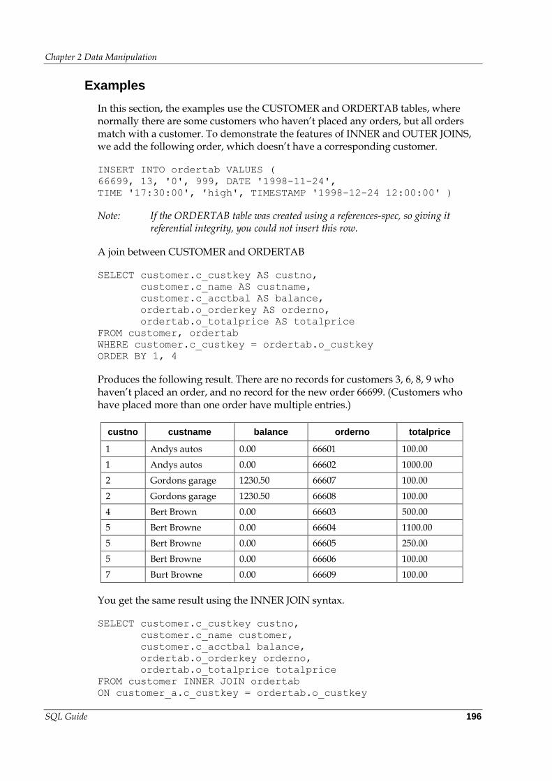
Chapter 2 Data Manipulation
SQL Guide 196
Examples
In this section, the examples use the CUSTOMER and ORDERTAB tables, where normally there are some customers who haven’t placed any orders, but all orders match with a customer. To demonstrate the features of INNER and OUTER JOINS, we add the following order, which doesn’t have a corresponding customer.
INSERT INTO ordertab VALUES (
66699, 13, '0', 999, DATE '1998-11-24',
TIME '17:30:00', 'high', TIMESTAMP '1998-12-24 12:00:00' )
Note: If the ORDERTAB table was created using a references-spec, so giving it referential integrity, you could not insert this row.
A join between CUSTOMER and ORDERTAB
SELECT customer.c_custkey AS custno,
customer.c_name AS custname,
customer.c_acctbal AS balance,
ordertab.o_orderkey AS orderno,
ordertab.o_totalprice AS totalprice
FROM customer, ordertab
WHERE customer.c_custkey = ordertab.o_custkey
ORDER BY 1, 4
Produces the following result. There are no records for customers 3, 6, 8, 9 who haven’t placed an order, and no record for the new order 66699. (Customers who have placed more than one order have multiple entries.)
custno custname balance orderno totalprice
1 Andys autos 0.00 66601 100.00
1 Andys autos 0.00 66602 1000.00
2 Gordons garage 1230.50 66607 100.00
2 Gordons garage 1230.50 66608 100.00
4 Bert Brown 0.00 66603 500.00
5 Bert Browne 0.00 66604 1100.00
5 Bert Browne 0.00 66605 250.00
5 Bert Browne 0.00 66606 100.00
7 Burt Browne 0.00 66609 100.00
You get the same result using the INNER JOIN syntax.
SELECT customer.c_custkey custno,
customer.c_name customer,
customer.c_acctbal balance,
ordertab.o_orderkey orderno,
ordertab.o_totalprice totalprice
FROM customer INNER JOIN ordertab
ON customer_a.c_custkey = ordertab.o_custkey
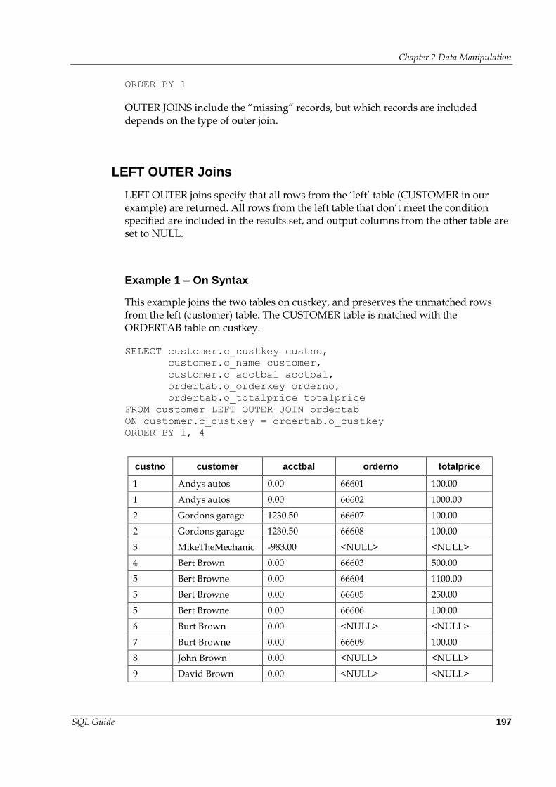
Chapter 2 Data Manipulation
SQL Guide 197
ORDER BY 1
OUTER JOINS include the “missing” records, but which records are included depends on the type of outer join.
LEFT OUTER Joins
LEFT OUTER joins specify that all rows from the ‘left’ table (CUSTOMER in our example) are returned. All rows from the left table that don’t meet the condition specified are included in the results set, and output columns from the other table are set to NULL.
Example 1 – On Syntax
This example joins the two tables on custkey, and preserves the unmatched rows from the left (customer) table. The CUSTOMER table is matched with the ORDERTAB table on custkey.
SELECT customer.c_custkey custno,
customer.c_name customer,
customer.c_acctbal acctbal,
ordertab.o_orderkey orderno,
ordertab.o_totalprice totalprice
FROM customer LEFT OUTER JOIN ordertab
ON customer.c_custkey = ordertab.o_custkey
ORDER BY 1, 4
custno customer acctbal orderno totalprice
1 Andys autos 0.00 66601 100.00
1 Andys autos 0.00 66602 1000.00
2 Gordons garage 1230.50 66607 100.00
2 Gordons garage 1230.50 66608 100.00
3 MikeTheMechanic -983.00 <NULL> <NULL>
4 Bert Brown 0.00 66603 500.00
5 Bert Browne 0.00 66604 1100.00
5 Bert Browne 0.00 66605 250.00
5 Bert Browne 0.00 66606 100.00
6 Burt Brown 0.00 <NULL> <NULL>
7 Burt Browne 0.00 66609 100.00
8 John Brown 0.00 <NULL> <NULL>
9 David Brown 0.00 <NULL> <NULL>
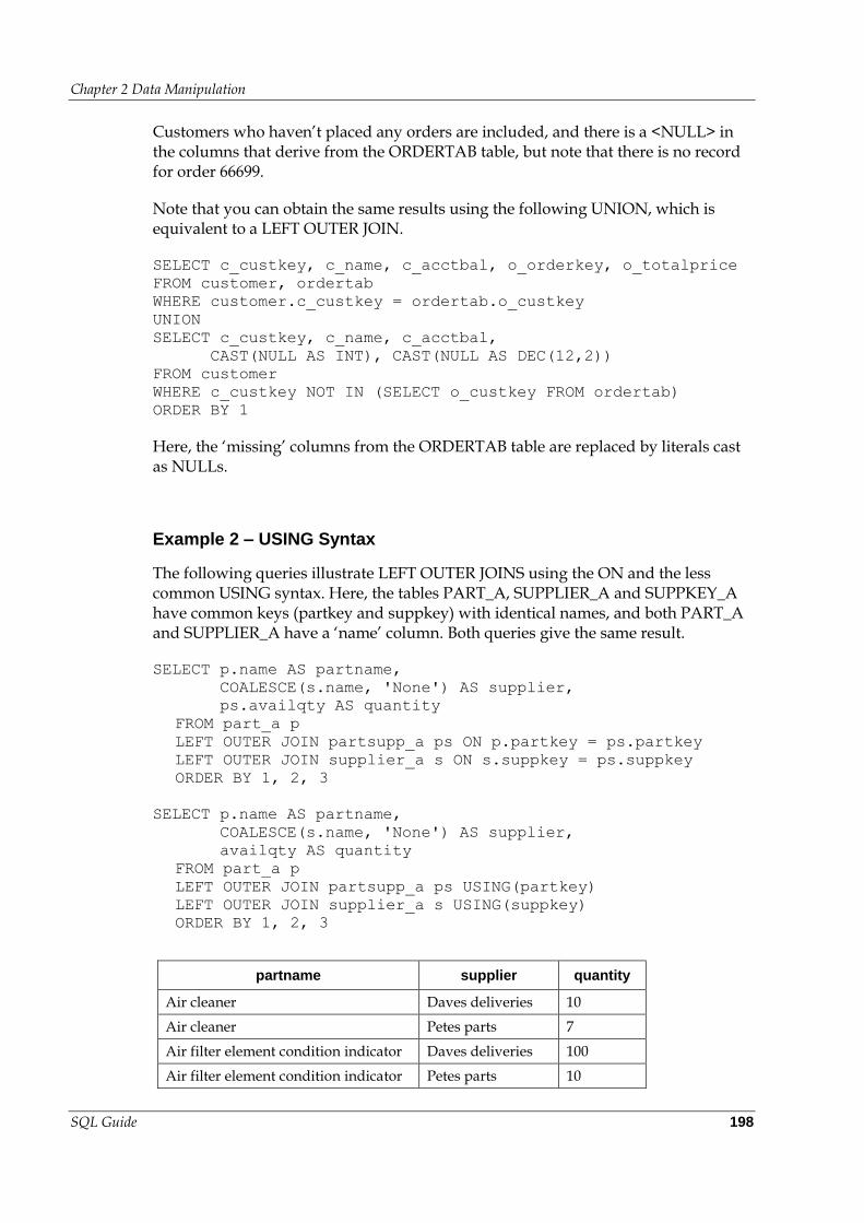
Chapter 2 Data Manipulation
SQL Guide 198
Customers who haven’t placed any orders are included, and there is a <NULL> in the columns that derive from the ORDERTAB table, but note that there is no record for order 66699.
Note that you can obtain the same results using the following UNION, which is equivalent to a LEFT OUTER JOIN.
SELECT c_custkey, c_name, c_acctbal, o_orderkey, o_totalprice
FROM customer, ordertab
WHERE customer.c_custkey = ordertab.o_custkey
UNION
SELECT c_custkey, c_name, c_acctbal,
CAST(NULL AS INT), CAST(NULL AS DEC(12,2))
FROM customer
WHERE c_custkey NOT IN (SELECT o_custkey FROM ordertab)
ORDER BY 1
Here, the ‘missing’ columns from the ORDERTAB table are replaced by literals cast as NULLs.
Example 2 – USING Syntax
The following queries illustrate LEFT OUTER JOINS using the ON and the less common USING syntax. Here, the tables PART_A, SUPPLIER_A and SUPPKEY_A have common keys (partkey and suppkey) with identical names, and both PART_A and SUPPLIER_A have a ‘name’ column. Both queries give the same result.
SELECT p.name AS partname,
COALESCE(s.name, 'None') AS supplier,
ps.availqty AS quantity
FROM part_a p
LEFT OUTER JOIN partsupp_a ps ON p.partkey = ps.partkey
LEFT OUTER JOIN supplier_a s ON s.suppkey = ps.suppkey
ORDER BY 1, 2, 3
SELECT p.name AS partname,
COALESCE(s.name, 'None') AS supplier,
availqty AS quantity
FROM part_a p
LEFT OUTER JOIN partsupp_a ps USING(partkey)
LEFT OUTER JOIN supplier_a s USING(suppkey)
ORDER BY 1, 2, 3
partname supplier quantity
Air cleaner Daves deliveries 10
Air cleaner Petes parts 7
Air filter element condition indicator Daves deliveries 100
Air filter element condition indicator Petes parts 10
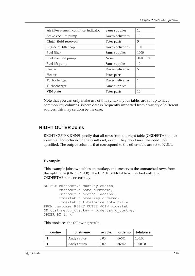
Chapter 2 Data Manipulation
SQL Guide 199
Air filter element condition indicator Sams supplies 10
Brake vacuum pump Daves deliveries 10
Clutch fluid reservoir Petes parts 5
Engine oil filler cap Daves deliveries 100
Fuel filter Sams supplies 1000
Fuel injection pump None <NULL>
Fuel lift pump Sams supplies 10
Heater Daves deliveries 5
Heater Petes parts 1
Turbocharger Daves deliveries 1
Turbocharger Sams supplies 1
VIN plate Petes parts 10
Note that you can only make use of this syntax if your tables are set up to have common key columns. Where data is frequently imported from a variety of different sources, this may seldom be the case.
RIGHT OUTER Joins
RIGHT OUTER JOINS specify that all rows from the right table (ORDERTAB in our example) are included in the results set, even if they don’t meet the condition specified. The output columns that correspond to the other table are set to NULL.
Example
This example joins two tables on custkey, and preserves the unmatched rows from the right table (ORDERTAB). The CUSTOMER table is matched with the ORDERTAB table on custkey.
SELECT customer.c_custkey custno,
customer.c_name custname,
customer.c_acctbal acctbal,
ordertab.o_orderkey orderno,
ordertab.o_totalprice totalprice
FROM customer RIGHT OUTER JOIN ordertab
ON customer.c_custkey = ordertab.o_custkey
ORDER BY 1, 4
This produces the following result.
custno custname acctbal orderno totalprice
1 Andys autos 0.00 66601 100.00
1 Andys autos 0.00 66602 1000.00
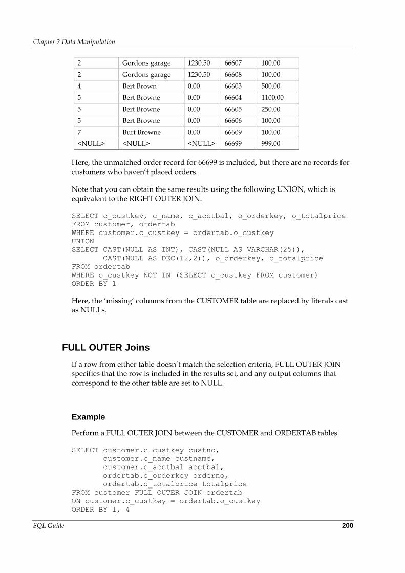
Chapter 2 Data Manipulation
SQL Guide 200
2 Gordons garage 1230.50 66607 100.00
2 Gordons garage 1230.50 66608 100.00
4 Bert Brown 0.00 66603 500.00
5 Bert Browne 0.00 66604 1100.00
5 Bert Browne 0.00 66605 250.00
5 Bert Browne 0.00 66606 100.00
7 Burt Browne 0.00 66609 100.00
<NULL> <NULL> <NULL> 66699 999.00
Here, the unmatched order record for 66699 is included, but there are no records for customers who haven’t placed orders.
Note that you can obtain the same results using the following UNION, which is equivalent to the RIGHT OUTER JOIN.
SELECT c_custkey, c_name, c_acctbal, o_orderkey, o_totalprice
FROM customer, ordertab
WHERE customer.c_custkey = ordertab.o_custkey
UNION
SELECT CAST(NULL AS INT), CAST(NULL AS VARCHAR(25)),
CAST(NULL AS DEC(12,2)), o_orderkey, o_totalprice
FROM ordertab
WHERE o_custkey NOT IN (SELECT c_custkey FROM customer)
ORDER BY 1
Here, the ‘missing’ columns from the CUSTOMER table are replaced by literals cast as NULLs.
FULL OUTER Joins
If a row from either table doesn’t match the selection criteria, FULL OUTER JOIN specifies that the row is included in the results set, and any output columns that correspond to the other table are set to NULL.
Example
Perform a FULL OUTER JOIN between the CUSTOMER and ORDERTAB tables.
SELECT customer.c_custkey custno,
customer.c_name custname,
customer.c_acctbal acctbal,
ordertab.o_orderkey orderno,
ordertab.o_totalprice totalprice
FROM customer FULL OUTER JOIN ordertab
ON customer.c_custkey = ordertab.o_custkey
ORDER BY 1, 4
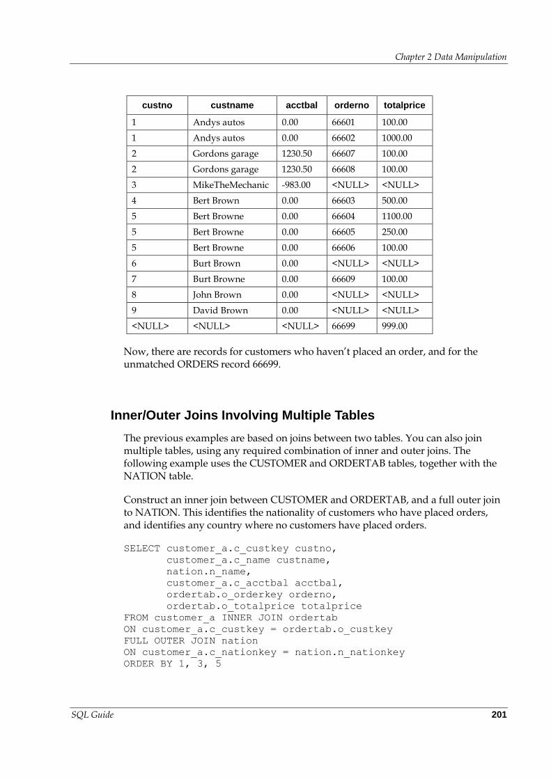
Chapter 2 Data Manipulation
SQL Guide 201
custno custname acctbal orderno totalprice
1 Andys autos 0.00 66601 100.00
1 Andys autos 0.00 66602 1000.00
2 Gordons garage 1230.50 66607 100.00
2 Gordons garage 1230.50 66608 100.00
3 MikeTheMechanic -983.00 <NULL> <NULL>
4 Bert Brown 0.00 66603 500.00
5 Bert Browne 0.00 66604 1100.00
5 Bert Browne 0.00 66605 250.00
5 Bert Browne 0.00 66606 100.00
6 Burt Brown 0.00 <NULL> <NULL>
7 Burt Browne 0.00 66609 100.00
8 John Brown 0.00 <NULL> <NULL>
9 David Brown 0.00 <NULL> <NULL>
<NULL> <NULL> <NULL> 66699 999.00
Now, there are records for customers who haven’t placed an order, and for the unmatched ORDERS record 66699.
Inner/Outer Joins Involving Multiple Tables
The previous examples are based on joins between two tables. You can also join multiple tables, using any required combination of inner and outer joins. The following example uses the CUSTOMER and ORDERTAB tables, together with the NATION table.
Construct an inner join between CUSTOMER and ORDERTAB, and a full outer join to NATION. This identifies the nationality of customers who have placed orders, and identifies any country where no customers have placed orders.
SELECT customer_a.c_custkey custno,
customer_a.c_name custname,
nation.n_name,
customer_a.c_acctbal acctbal,
ordertab.o_orderkey orderno,
ordertab.o_totalprice totalprice
FROM customer_a INNER JOIN ordertab
ON customer_a.c_custkey = ordertab.o_custkey
FULL OUTER JOIN nation
ON customer_a.c_nationkey = nation.n_nationkey
ORDER BY 1, 3, 5
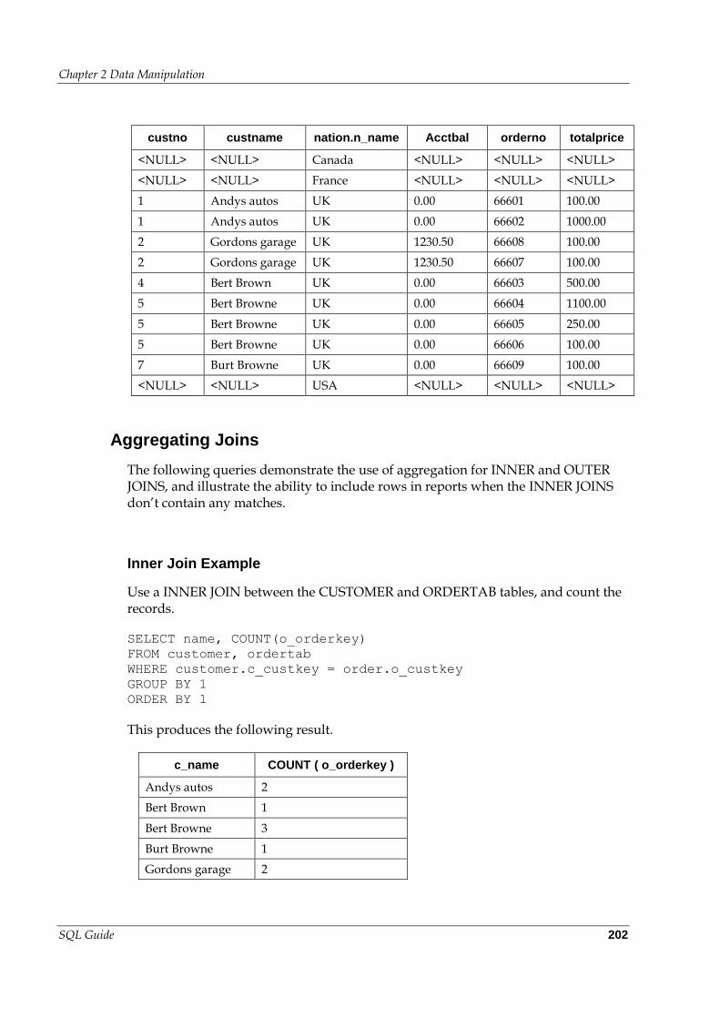
Chapter 2 Data Manipulation
SQL Guide 202
custno custname nation.n_name Acctbal orderno totalprice
<NULL> <NULL> Canada <NULL> <NULL> <NULL>
<NULL> <NULL> France <NULL> <NULL> <NULL>
1 Andys autos UK 0.00 66601 100.00
1 Andys autos UK 0.00 66602 1000.00
2 Gordons garage UK 1230.50 66608 100.00
2 Gordons garage UK 1230.50 66607 100.00
4 Bert Brown UK 0.00 66603 500.00
5 Bert Browne UK 0.00 66604 1100.00
5 Bert Browne UK 0.00 66605 250.00
5 Bert Browne UK 0.00 66606 100.00
7 Burt Browne UK 0.00 66609 100.00
<NULL> <NULL> USA <NULL> <NULL> <NULL>
Aggregating Joins
The following queries demonstrate the use of aggregation for INNER and OUTER JOINS, and illustrate the ability to include rows in reports when the INNER JOINS don’t contain any matches.
Inner Join Example
Use a INNER JOIN between the CUSTOMER and ORDERTAB tables, and count the records.
SELECT name, COUNT(o_orderkey)
FROM customer, ordertab
WHERE customer.c_custkey = order.o_custkey
GROUP BY 1
ORDER BY 1
This produces the following result.
c_name COUNT ( o_orderkey )
Andys autos 2
Bert Brown 1
Bert Browne 3
Burt Browne 1
Gordons garage 2
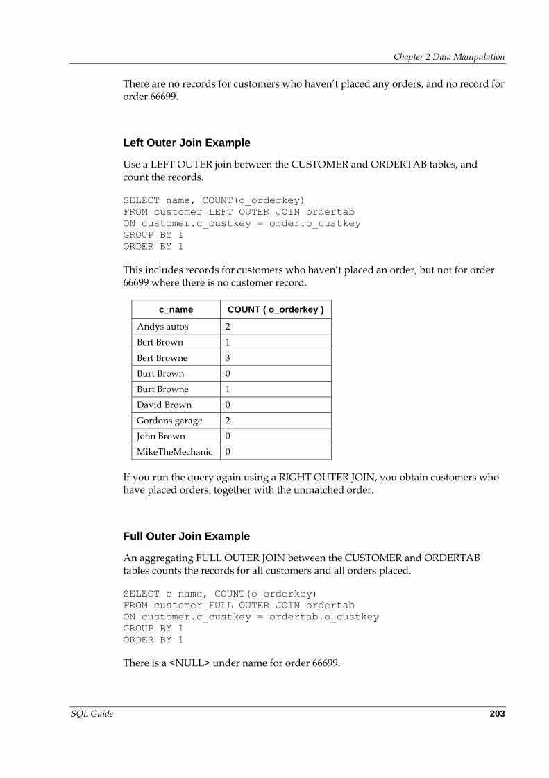
Chapter 2 Data Manipulation
SQL Guide 203
There are no records for customers who haven’t placed any orders, and no record for order 66699.
Left Outer Join Example
Use a LEFT OUTER join between the CUSTOMER and ORDERTAB tables, and count the records.
SELECT name, COUNT(o_orderkey)
FROM customer LEFT OUTER JOIN ordertab
ON customer.c_custkey = order.o_custkey
GROUP BY 1
ORDER BY 1
This includes records for customers who haven’t placed an order, but not for order 66699 where there is no customer record.
c_name COUNT ( o_orderkey )
Andys autos 2
Bert Brown 1
Bert Browne 3
Burt Brown 0
Burt Browne 1
David Brown 0
Gordons garage 2
John Brown 0
MikeTheMechanic 0
If you run the query again using a RIGHT OUTER JOIN, you obtain customers who have placed orders, together with the unmatched order.
Full Outer Join Example
An aggregating FULL OUTER JOIN between the CUSTOMER and ORDERTAB tables counts the records for all customers and all orders placed.
SELECT c_name, COUNT(o_orderkey)
FROM customer FULL OUTER JOIN ordertab
ON customer.c_custkey = ordertab.o_custkey
GROUP BY 1
ORDER BY 1
There is a <NULL> under name for order 66699.
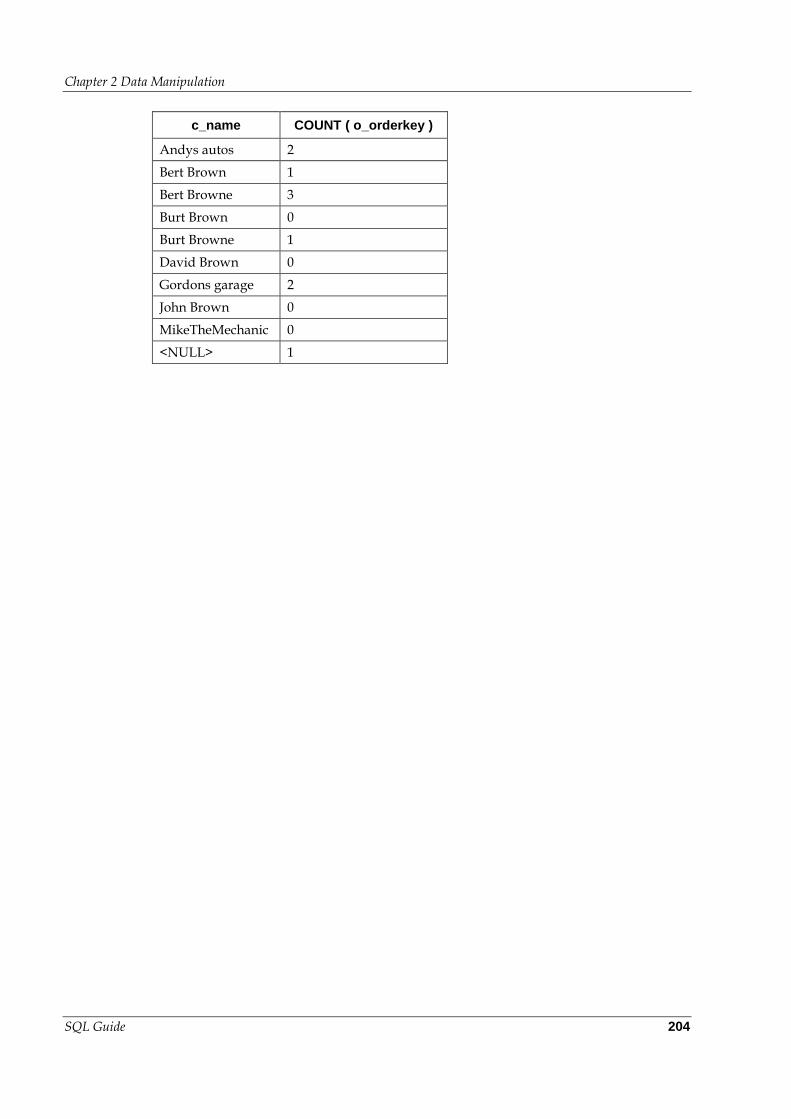
Chapter 2 Data Manipulation
SQL Guide 204
c_name COUNT ( o_orderkey )
Andys autos 2
Bert Brown 1
Bert Browne 3
Burt Brown 0
Burt Browne 1
David Brown 0
Gordons garage 2
John Brown 0
MikeTheMechanic 0
<NULL> 1
Kognitio SQL Guide 205
3
Connections and Transaction Control
This chapter discusses the way users connect to Kognitio systems and how SQL commands can be formed in to multi-statement transactions.
COMMIT
Use the COMMIT statement to commit changes made to the database tables since the start of the current transaction. COMMIT terminates the transaction.
Usage
COMMIT [WORK]
Notes
All locks are released on completing the COMMIT. You can use a ROLLBACK statement to reverse any changes made, in place of a COMMIT.
Example 1
To commit all work in the current transaction, use
COMMIT WORK
Or just
COMMIT
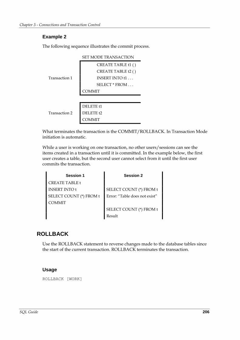
Chapter 3 - Connections and Transaction Control
SQL Guide 206
Example 2
The following sequence illustrates the commit process.
SET MODE TRANSACTION
Transaction 1
CREATE TABLE t1 ( )
CREATE TABLE t2 ( )
INSERT INTO t1 . . .
SELECT * FROM . . .
COMMIT
Transaction 2
DELETE t1
DELETE t2
COMMIT
What terminates the transaction is the COMMIT/ROLLBACK. In Transaction Mode initiation is automatic.
While a user is working on one transaction, no other users/sessions can see the items created in a transaction until it is committed. In the example below, the first user creates a table, but the second user cannot select from it until the first user commits the transaction.
Session 1 Session 2
CREATE TABLE t
INSERT INTO t SELECT COUNT (*) FROM t
SELECT COUNT (*) FROM t Error: “Table does not exist”
COMMIT
SELECT COUNT (*) FROM t
Result
ROLLBACK
Use the ROLLBACK statement to reverse changes made to the database tables since the start of the current transaction. ROLLBACK terminates the transaction.
Usage
ROLLBACK [WORK]
Chapter 3 - Connections and Transaction Control
SQL Guide 207
Notes
All locks are released on receiving the Rollback. Use a ROLLBACK statement to reverse any changes made within the transaction.
Note that rolling back may take some time, especially if multi-statements or large INSERTS or DELETES are involved.
Due to their nature, some operations cannot be rolled back; for example CREATE OR REPLACE VIEW IMAGE cannot be rolled back because the old image must be dropped, before the new image is created, otherwise there may be insufficient RAM to store the old and new images simultaneously. The types of operations that cannot be rolled back are the large-scale maintenance operations, for example:
RECREATE INVALIDATED VIEWS
ALTER TABLE CASCADE
CREATE OR REPLACE VIEW
CREATE SEC CLASS
ALTER SEC CLASS
CREATE IMAGE
RECLAIM
CREATE PLUGIN
ALTER PLUGIN
DROP PLUGIN
Example
To rollback from the start of the current transaction, use
ROLLBACK WORK
Or just
ROLLBACK
SET MODE
Use SET MODE to determine the current transaction mode. The following modes are supported
AUTOCOMMIT
TRANSACTION.
Chapter 3 - Connections and Transaction Control
SQL Guide 208
Usage
SET MODE {AUTOCOMMIT | TRANSACTION}
Notes
In AUTOCOMMIT mode, all transactions are automatically committed after each individual SQL statement, unless an error occurs—in which case they are rolled back.
In TRANSACTION mode, a transaction starts either after the first command is received and/or after subsequent COMMIT or ROLLBACK commands.
CONNECT
Use the CONNECT statement to make the connection to a specified Kognitio, using a given identity and password.
Usage
CONNECT TO server USER user USING | PASSWORD password
Notes
Most PC applications provide a dialog box to allow you to specify server, user and password. It is also possible to type in the CONNECT command directly in those applications that allow SQL to be typed in and submitted (e.g. QuerySTUDIO and LaunchPad). Other applications (typically Unix ones) allow the option of specifying the connection parameters on the command-line.
Connecting through a login dialog box has the in-built advantage that your password is kept secret throughout your connection.
Note that issuing a CONNECT when already connected is equivalent to
DISCONNECT
CONNECT
Regardless of whether the connection is to the same or a different Kognitio.
Chapter 3 - Connections and Transaction Control
SQL Guide 209
Example
To connect to the Kognitio called “TELCO”, using the identity “TELCO_WORKER” and the password “t3lc0”, use
CONNECT TO TELCO USER TELCO_WORKER USING T3LC0
As the case used isn’t significant, you can also make the connection by entering
connect to telco user telco_worker using t3lc0
You either connect successfully, or get an error message. For security reasons, the message resulting from an invalid user name or password doesn’t indicate whether it is the user or the password portion that is incorrect.
DISCONNECT
Once a session is complete, you need to terminate the connection to the specified Kognitio. Do this using the DISCONNECT command.
Usage
DISCONNECT
Notes
This terminates the current session, and closes the connection to Kognitio.

Kognitio SQL Guide 211
4
Privileges
This chapter introduces privileges and shows how they are granted and revoked from users and groups.
4.1 Privileges
On Kognitio, security is achieved through the combination of a user name, password and privileges. Privileges are an underlying feature, and define the access each user has to
Data (to ensure security and integrity)
Commands that affect overall performance and system availability for all users.
User names, passwords and privileges are recorded in the system tables, which are set up when Kognitio is installed.
You need privileges to
Access columns in tables and views
Execute certain SQL commands, for example, CREATE IMAGE, DROP TABLE.
All privileges derive from the user identity SYS—probably your System Administrator. SYS grants certain privileges when registering a new user, and has privileges on all tables in the system—both system tables, and tables created by other users. SYS can change a user's privileges as the need arises.
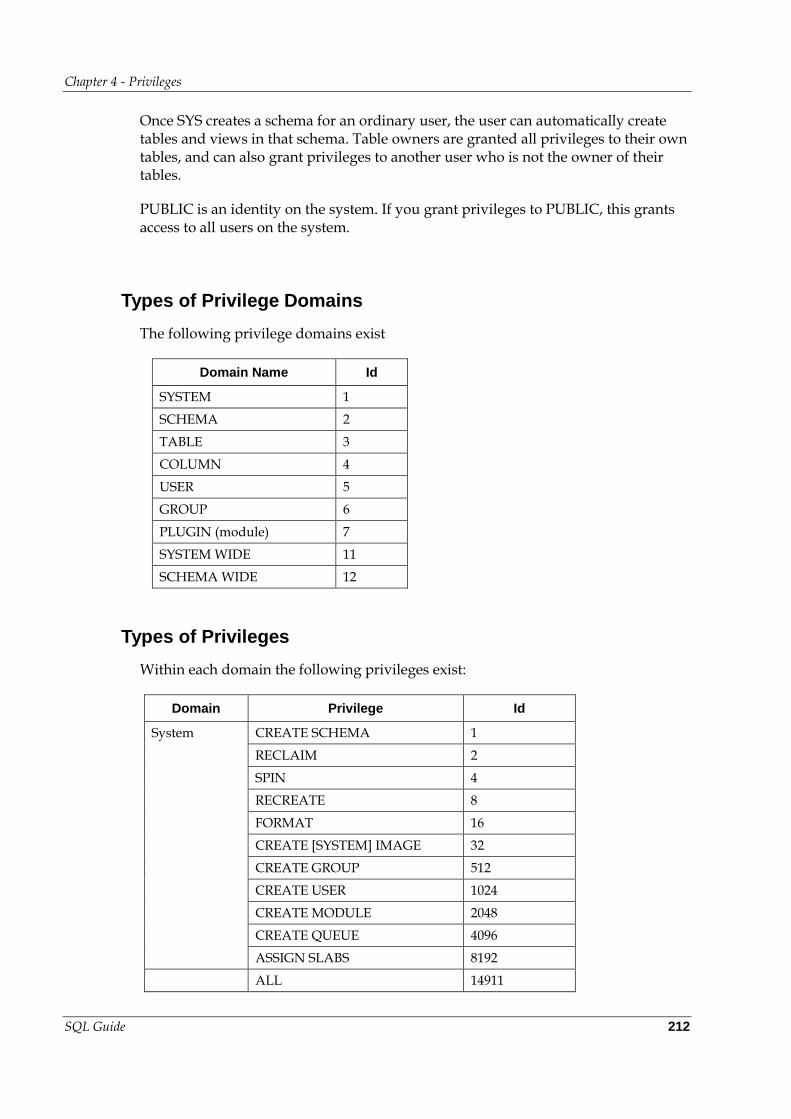
Chapter 4 - Privileges
SQL Guide 212
Once SYS creates a schema for an ordinary user, the user can automatically create tables and views in that schema. Table owners are granted all privileges to their own tables, and can also grant privileges to another user who is not the owner of their tables.
PUBLIC is an identity on the system. If you grant privileges to PUBLIC, this grants access to all users on the system.
Types of Privilege Domains
The following privilege domains exist
Domain Name Id
SYSTEM 1
SCHEMA 2
TABLE 3
COLUMN 4
USER 5
GROUP 6
PLUGIN (module) 7
SYSTEM WIDE 11
SCHEMA WIDE 12
Types of Privileges
Within each domain the following privileges exist:
Domain Privilege Id
System CREATE SCHEMA 1
RECLAIM 2
SPIN 4
RECREATE 8
FORMAT 16
CREATE [SYSTEM] IMAGE 32
CREATE GROUP 512
CREATE USER 1024
CREATE MODULE 2048
CREATE QUEUE 4096
ASSIGN SLABS 8192
ALL 14911
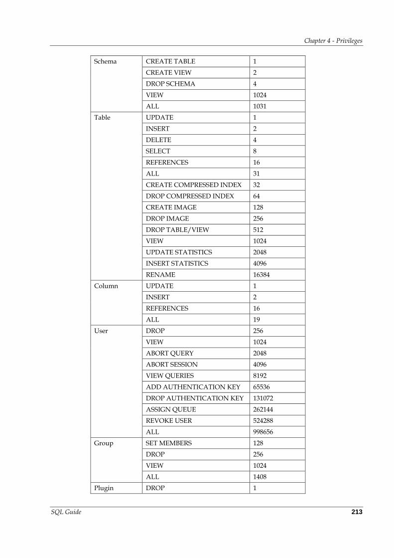
Chapter 4 - Privileges
SQL Guide 213
Schema CREATE TABLE 1
CREATE VIEW 2
DROP SCHEMA 4
VIEW 1024
ALL 1031
Table UPDATE 1
INSERT 2
DELETE 4
SELECT 8
REFERENCES 16
ALL 31
CREATE COMPRESSED INDEX 32
DROP COMPRESSED INDEX 64
CREATE IMAGE 128
DROP IMAGE 256
DROP TABLE/VIEW 512
VIEW 1024
UPDATE STATISTICS 2048
INSERT STATISTICS 4096
RENAME 16384
Column UPDATE 1
INSERT 2
REFERENCES 16
ALL 19
User DROP 256
VIEW 1024
ABORT QUERY 2048
ABORT SESSION 4096
VIEW QUERIES 8192
ADD AUTHENTICATION KEY 65536
DROP AUTHENTICATION KEY 131072
ASSIGN QUEUE 262144
REVOKE USER 524288
ALL 998656
Group SET MEMBERS 128
DROP 256
VIEW 1024
ALL 1408
Plugin DROP 1
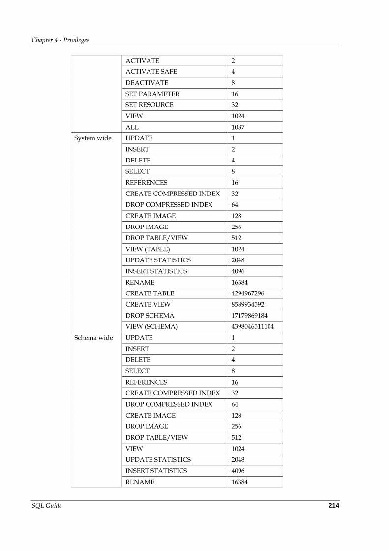
Chapter 4 - Privileges
SQL Guide 214
ACTIVATE 2
ACTIVATE SAFE 4
DEACTIVATE 8
SET PARAMETER 16
SET RESOURCE 32
VIEW 1024
ALL 1087
System wide UPDATE 1
INSERT 2
DELETE 4
SELECT 8
REFERENCES 16
CREATE COMPRESSED INDEX 32
DROP COMPRESSED INDEX 64
CREATE IMAGE 128
DROP IMAGE 256
DROP TABLE/VIEW 512
VIEW (TABLE) 1024
UPDATE STATISTICS 2048
INSERT STATISTICS 4096
RENAME 16384
CREATE TABLE 4294967296
CREATE VIEW 8589934592
DROP SCHEMA 17179869184
VIEW (SCHEMA) 4398046511104
Schema wide UPDATE 1
INSERT 2
DELETE 4
SELECT 8
REFERENCES 16
CREATE COMPRESSED INDEX 32
DROP COMPRESSED INDEX 64
CREATE IMAGE 128
DROP IMAGE 256
DROP TABLE/VIEW 512
VIEW 1024
UPDATE STATISTICS 2048
INSERT STATISTICS 4096
RENAME 16384
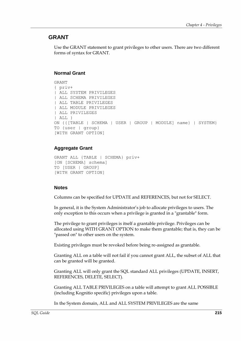
Chapter 4 - Privileges
SQL Guide 215
GRANT
Use the GRANT statement to grant privileges to other users. There are two different forms of syntax for GRANT.
Normal Grant
GRANT
{ priv+
| ALL SYSTEM PRIVILEGES
| ALL SCHEMA PRIVILEGES
| ALL TABLE PRIVILEGES
| ALL MODULE PRIVILEGES
| ALL PRIVILEGES
| ALL }
ON {{[TABLE | SCHEMA | USER | GROUP | MODULE] name} | SYSTEM}
TO {user | group}
[WITH GRANT OPTION]
Aggregate Grant
GRANT ALL {TABLE | SCHEMA} priv+
[ON [SCHEMA] schema]
TO [USER | GROUP]
[WITH GRANT OPTION]
Notes
Columns can be specified for UPDATE and REFERENCES, but not for SELECT.
In general, it is the System Administrator’s job to allocate privileges to users. The only exception to this occurs when a privilege is granted in a "grantable" form.
The privilege to grant privileges is itself a grantable privilege. Privileges can be allocated using WITH GRANT OPTION to make them grantable; that is, they can be "passed on" to other users on the system.
Existing privileges must be revoked before being re-assigned as grantable.
Granting ALL on a table will not fail if you cannot grant ALL, the subset of ALL that can be granted will be granted.
Granting ALL will only grant the SQL standard ALL privileges (UPDATE, INSERT, REFERENCES, DELETE, SELECT).
Granting ALL TABLE PRIVILEGES on a table will attempt to grant ALL POSSIBLE (including Kognitio specific) privileges upon a table.
In the System domain, ALL and ALL SYSTEM PRIVILEGES are the same
Chapter 4 - Privileges
SQL Guide 216
In the Schema domain, ALL and ALL SCHEMA PRIVILEGES are the same
In the User domain, ALL and ALL USER PRIVILEGES are the same
In the Group domain, ALL and ALL GROUP PRIVILEGES are the same
Clearly, granting an ALL SCHEMA privilege is only useful if we are granting a privilege on all schemas in the system.
If granting an ALL TABLE privilege, it can either be on every table in the system, or on every table in a schema. If the latter, then [ON [SCHEMA] schema] should be provided.
Possession of an aggregate privilege with grant option does not allow implied privileges to be granted; if FRED has all table drop on schema S1 with grant option, then he cannot grant drop on a specific table in S1, only the aggregate privilege.
UPDATE privilege does not imply SELECT privilege. To successfully perform a command of the form “UPDATE T1 SET C1 = X WHERE C1 < 0”, both UPDATE and SELECT privileges must be granted to the user on T1. A similar condition also applies to column-wide privileges.
Privileges are discussed in detail in the Kognitio Guide.
Example 1 – Granting Standard Privileges
Grant users with the identifiers JOHN_SMITH and LIBERTYM both SELECT and UPDATE access to the CUSTOMER table, and allow them to grant these privileges to other users at their discretion.
GRANT SELECT, UPDATE
ON customer
TO JOHN_SMITH, LIBERTYM WITH GRANT OPTION
Example 2 – Granting Update Privileges on Specific Columns
Grant update privileges on specific columns.
GRANT UPDATE(c_address, c_postcode, c_phone)
ON customer
TO JOHN_SMITH
Example 3 – Granting a Kognitio Privilege
Grant the Kognitio privileges DROP TABLE, DROP VIEW, CREATE IMAGE and DROP IMAGE on the CUSTOMER table to JOHN_SMITH.
GRANT DROP TABLE, DROP VIEW, CREATE IMAGE, DROP IMAGE
Chapter 4 - Privileges
SQL Guide 217
ON customer
TO JOHN_SMITH
Example 4 – Granting View and Abort Privileges
This example allows user TRAINER to see and abort Kognitio queries and sessions being run by the user TRAINEE.
GRANT ABORT SESSION ON USER trainee TO trainer
GRANT ABORT QUERY ON USER trainee TO trainer
GRANT VIEW QUERIES ON USER trainee TO trainer
There is actually no reason why this needs to be three separate statements or why the privileges cannot be granted to a group, e.g.
GRANT ABORT SESSION, ABORT QUERY, VIEW QUERIES
ON USER trainee TO trainer_group
REVOKE
Use the REVOKE statement to remove privileges previously granted to selected users. There are two different forms of syntax for REVOKE.
Normal Revoke
REVOKE
[GRANT OPTION FOR]
{ priv+
| ALL SYSTEM PRIVILEGES
| ALL SCHEMA PRIVILEGES
| ALL TABLE PRIVILEGES
| ALL PRIVILEGES
| ALL }
ON {{[TABLE | SCHEMA | USER | GROUP | MODULE] name} | SYSTEM}
FROM {user | group}
Aggregate Revoke
REVOKE [GRANT OPTION FOR] ALL { TABLE | SCHEMA } priv+
[ON [SCHEMA] schema]
FROM [USER | GROUP]
Chapter 4 - Privileges
SQL Guide 218
Notes
Usually, it is the System Administrator’s job to allocate privileges to users, so, it is usually the System Administrator who revokes a user’s privileges.
Revoking privileges on a given table removes any privileges previously granted on selected columns in that table. However, individual column-based privileges can also be revoked.
Example 1 – Revoking a Standard Privilege
To revoke the privileges granted in Grant: Example 1.
REVOKE SELECT, UPDATE
ON sales_reps
FROM JOHN_SMITH, LIBERTYM
Example 2 – Revoking Privileges on Selected Columns in a Table
Revoke privileges on selected columns within a table.
REVOKE UPDATE(c_acctbal, c_flags)
ON customer
FROM LIBERTYM
Example 3 – Revoking the Grant Option on a Kognitio Privileges
Revoke the grant option on the Kognitio drop table privileges on the CUSTOMER table from LIBERTYM.
REVOKE GRANT OPTION FOR DROP TABLE
ON customer
FROM LIBERTYM
Kognitio SQL Guide 219
5
Users and Groups
This chapter introduces the concept of placing users in hierarchical groups to simplify privilege control and data access. It also discusses how groups and users are created.
5.1 Overview
On a Kognitio system all users belong to one or more groups. A PUBLIC group is created when Kognitio is installed, and all users belong to it. The user with SYS privileges, normally the System Administrator, creates other groups. Groups are defined as follows.
Groups share the user namespace and user id space; no user can have the same name or id as a group and vice versa.
Any permission that can be granted to a user can also be granted to a group. Grantable permissions can also be assigned to a group.
Groups can be members of other groups. This relationship can be cyclic (that is, Group A is in Group B, which is in group C, which is in Group A).
A user has an effective permission on an object if they are a member of any group that has the permission. Likewise a group has an effective permission if it is a member of any group that has a permission and so on. Effective permissions are used to access an object, but not for grant/revoke. This means that if a user X is in group Y and Y has select on a table T, X will be able to select from T because the user has effective permission. The user doesn’t actually have the permission, so REVOKE SELECT ON T FROM X will fail.
Groups can only be created and dropped by a user with SYS privileges. Users can only be added/removed from groups by a user with SYS privileges.
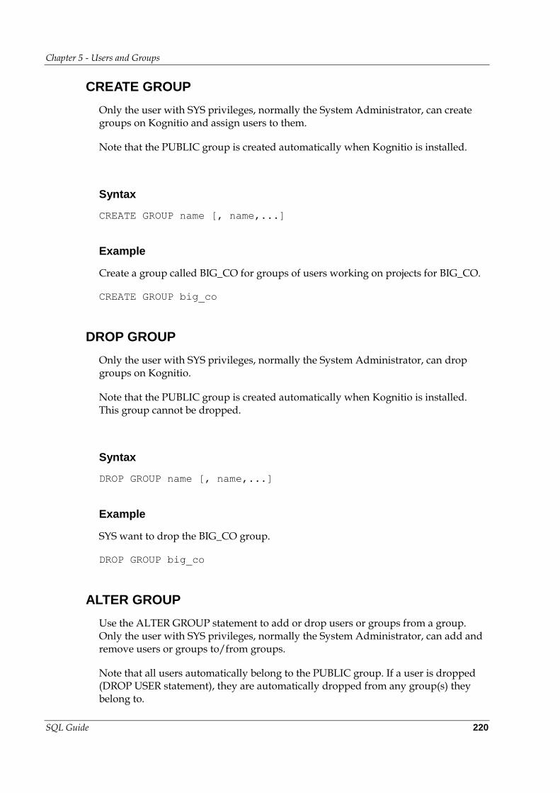
Chapter 5 - Users and Groups
SQL Guide 220
CREATE GROUP
Only the user with SYS privileges, normally the System Administrator, can create groups on Kognitio and assign users to them.
Note that the PUBLIC group is created automatically when Kognitio is installed.
Syntax
CREATE GROUP name [, name,...]
Example
Create a group called BIG_CO for groups of users working on projects for BIG_CO.
CREATE GROUP big_co
DROP GROUP
Only the user with SYS privileges, normally the System Administrator, can drop groups on Kognitio.
Note that the PUBLIC group is created automatically when Kognitio is installed. This group cannot be dropped.
Syntax
DROP GROUP name [, name,...]
Example
SYS want to drop the BIG_CO group.
DROP GROUP big_co
ALTER GROUP
Use the ALTER GROUP statement to add or drop users or groups from a group. Only the user with SYS privileges, normally the System Administrator, can add and remove users or groups to/from groups.
Note that all users automatically belong to the PUBLIC group. If a user is dropped (DROP USER statement), they are automatically dropped from any group(s) they belong to.
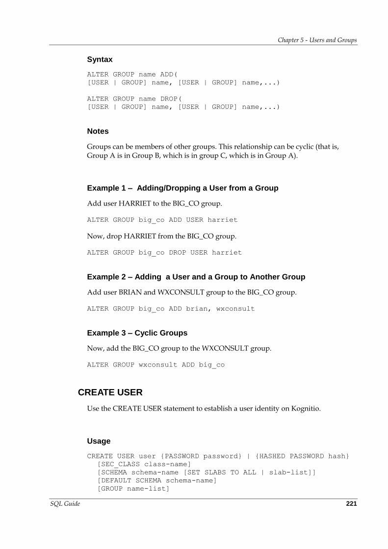
Chapter 5 - Users and Groups
SQL Guide 221
Syntax
ALTER GROUP name ADD(
[USER | GROUP] name, [USER | GROUP] name,...)
ALTER GROUP name DROP(
[USER | GROUP] name, [USER | GROUP] name,...)
Notes
Groups can be members of other groups. This relationship can be cyclic (that is, Group A is in Group B, which is in group C, which is in Group A).
Example 1 – Adding/Dropping a User from a Group
Add user HARRIET to the BIG_CO group.
ALTER GROUP big_co ADD USER harriet
Now, drop HARRIET from the BIG_CO group.
ALTER GROUP big_co DROP USER harriet
Example 2 – Adding a User and a Group to Another Group
Add user BRIAN and WXCONSULT group to the BIG_CO group.
ALTER GROUP big_co ADD brian, wxconsult
Example 3 – Cyclic Groups
Now, add the BIG_CO group to the WXCONSULT group.
ALTER GROUP wxconsult ADD big_co
CREATE USER
Use the CREATE USER statement to establish a user identity on Kognitio.
Usage
CREATE USER user {PASSWORD password} | {HASHED PASSWORD hash}
[SEC_CLASS class-name]
[SCHEMA schema-name [SET SLABS TO ALL | slab-list]]
[DEFAULT SCHEMA schema-name]
[GROUP name-list]
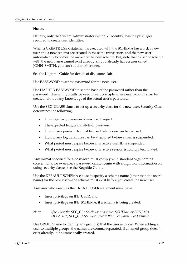
Chapter 5 - Users and Groups
SQL Guide 222
Notes
Usually, only the System Administrator (with SYS identity) has the privileges required to create user identities.
When a CREATE USER statement is executed with the SCHEMA keyword, a new user and a new schema are created in the same transaction, and the new user automatically becomes the owner of the new schema. But, note that a user or schema with the new name cannot exist already. (If you already have a user called JOHN_SMITH, you can’t add another one).
See the Kognitio Guide for details of disk store slabs.
Use PASSWORD to set the password for the new user.
Use HASHED PASSWORD to set the hash of the password rather than the password. This will typically be used in setup scripts where user accounts can be created without any knowledge of the actual user’s password.
Use the SEC_CLASS clause to set up a security class for the new user. Security Class determines the following.
How regularly passwords must be changed.
The expected length and style of password.
How many passwords must be used before one can be re-used.
How many log in failures can be attempted before a user is suspended.
What period must expire before an inactive user ID is suspended.
What period must expire before an inactive session is forcibly terminated.
Any format specified for a password must comply with standard SQL naming conventions; for example, a password cannot begin with a digit. For information on using security classes see the Kognitio Guide.
Use the DEFAULT SCHEMA clause to specify a schema name (other than the user’s name) for the new user—the schema must exist before you create the new user.
Any user who executes the CREATE USER statement must have
Insert privilege on IPE_USER, and
Insert privilege on IPE_SCHEMA, if a schema is being created.
Note: If you use the SEC_CLASS clause and either SCHEMA or SCHEMA DEFAULT, SEC_CLASS must precede the other clause. See Example 3.
Use GROUP name to identify any group(s) that the user is to join. When adding a user to multiple groups, the names are comma-separated. If a named group doesn’t exist already, it is automatically created.
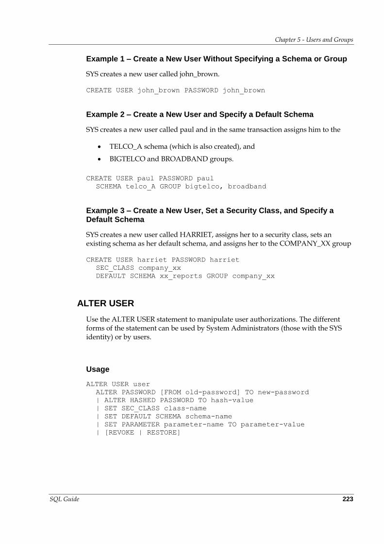
Chapter 5 - Users and Groups
SQL Guide 223
Example 1 – Create a New User Without Specifying a Schema or Group
SYS creates a new user called john_brown.
CREATE USER john_brown PASSWORD john_brown
Example 2 – Create a New User and Specify a Default Schema
SYS creates a new user called paul and in the same transaction assigns him to the
TELCO_A schema (which is also created), and
BIGTELCO and BROADBAND groups.
CREATE USER paul PASSWORD paul
SCHEMA telco_A GROUP bigtelco, broadband
Example 3 – Create a New User, Set a Security Class, and Specify a Default Schema
SYS creates a new user called HARRIET, assigns her to a security class, sets an existing schema as her default schema, and assigns her to the COMPANY_XX group
CREATE USER harriet PASSWORD harriet
SEC_CLASS company_xx
DEFAULT SCHEMA xx_reports GROUP company_xx
ALTER USER
Use the ALTER USER statement to manipulate user authorizations. The different forms of the statement can be used by System Administrators (those with the SYS identity) or by users.
Usage
ALTER USER user
ALTER PASSWORD [FROM old-password] TO new-password
| ALTER HASHED PASSWORD TO hash-value
| SET SEC_CLASS class-name
| SET DEFAULT SCHEMA schema-name
| SET PARAMETER parameter-name TO parameter-value
| [REVOKE | RESTORE]
Chapter 5 - Users and Groups
SQL Guide 224
Notes
When using the ALTER USER statement, you can only change one option at a time. For example, the System Administrator cannot alter a user’s password and security class at the same time.
Use the ALTER PASSWORD clause to change password. As explained below, the syntax varies depending on whether you have Update privilege on the System table IPE_USER.
Use ALTER HASHED PASSWORD to alter the hash of the password rather than the password. This will typically be used in setup scripts where user accounts can be created without any knowledge of the actual user’s password.
Use the SET SEC_CLASS clause to change the security class for a user. General information on parameters controlled by security class is given with the CREATE USER command. Additional information on setting up and using security classes is given in the Kognitio Guide.
Use the SET DEFAULT SCHEMA clause to change the default schema for a user. The schema must exist already.
Use REVOKE to deny access to Kognitio for a specific user, so they cannot log on. Any attempt to log on, results in the error message
S1000: [Kognitio][9800 Series Driver]
AM0026: Login has been revoked
SYS can restore a user's privilege to logon using RESTORE.
Only users with UPDATE privileges on IPE_USER can use the SEC_CLASS, REVOKE and RESTORE options.
Users without UPDATE privilege on IPE_USER who want to alter their own password require a FROM clause, when using the ALTER PASSWORD clause. See Example 2.
Note: Unlike many operating systems you do not confirm the password on Kognitio. Also, since ALTER USER is just an SQL command, the passwords are echoed in a readable form.
If the default schema is being changed, then the issuing user must be the same as the affected user, or the issuing user must have UPDATE privilege on IPE_USER.
System Administrators can modify any user password without needing to know the existing password. This requires UPDATE privilege on the system table IPE_USER.
Only the SYS user can alter a user’s parameters or their password hash value.
An authorized user can change their own password without requiring further privileges.
Chapter 5 - Users and Groups
SQL Guide 225
Case Sensitivity
Both user name and password are converted into upper case before further processing, so they are case insensitive when used in commands. User passwords are stored by Kognitio in encrypted form, in a table that only the System Administrator can access (by default). (Note that System Administrators can only see the encrypted form of passwords.)
The class-name is not case sensitive, but is stored internally in upper case. Information on setting up and using security classes is given the Kognitio Guide. General information on parameters controlled by security class is given with the CREATE USER command.
Example 1 – SYS Changes USER Harriet’s Password
SYS wishes to change the password for user Harriet. Note that SYS doesn’t need to know Harriet’s password.
ALTER USER harriet ALTER PASSWORD TO r3m3mb3rit
Example 2 – User Harriet Changes Her Own Password
User Harriet, who doesn’t have Update privilege on IPE_USER, can alter her own password, but note that she requires a FROM clause to identify her old password. Harriet must first log on using the old password, then issue the command.
ALTER USER harriet
ALTER PASSWORD FROM r3m3mb3rit to d0ntf0rg3t
Example 3 – Changing a User’s Default Schema
SYS wants to change the default schema for user Marcus. Note that the new default schema must already exist.
ALTER USER marcus SET DEFAULT SCHEMA telco_data
Example 4 – Revoking and Restoring the Login Privilege
User HARRIET is a temporary worker, whose current contract has come to an end. SYS wants to prevent her from logging in until a new contract is in place.
ALTER USER harriet REVOKE
Once this command it given, HARRIET will receive the error message, "AM0026: Login has been revoked", if she attempts to log in. SYS can restore login privileges with the following command.
Chapter 5 - Users and Groups
SQL Guide 226
ALTER USER harriet RESTORE
DROP USER
Use the DROP USER statement to remove a user from the list of authorized users.
Usage
DROP USER user
Notes
Usually, only the System Administrator (with SYS identity) has the necessary privileges to remove user identities.
Dropping a user doesn’t remove their tables, or any schema bearing their identity, from the database. However, it does drop the user from any group(s) they belong to.
Kognitio SQL Guide 227
6
Data Administrative Functions
This chapter discusses various administration commands including Importing and Exporting data, reclaiming disk space, gathering statistics, generating Compressed Data Maps and investigating how SQL will be executed on Kognitio.
6.1 Explain, Picture and Diagnose
EXPLAIN
You can precede an SQL statement with EXPLAIN, to produce text output explaining how the optimizer will handle the command or request. EXPLAIN is discussed in detail in the Kognitio Guide.
You can also obtain information about an object (id, image information, column details, etc.) and any views that depend on an object.
Usage
EXPLAIN query-statement
EXPLAIN object-name [DEPENDENT VIEWS | CASCADE]
Notes
The query is not executed by Kognitio, when preceded by EXPLAIN, rather the optimizer's execution plan for it is returned.
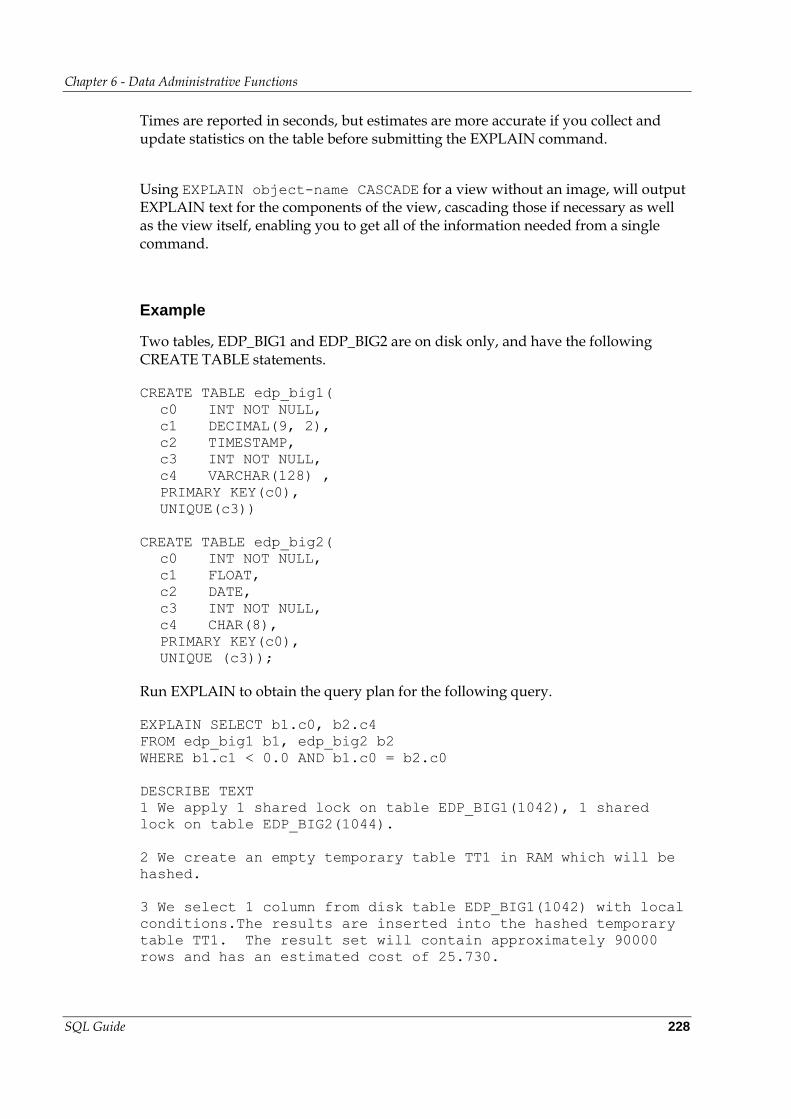
Chapter 6 - Data Administrative Functions
SQL Guide 228
Times are reported in seconds, but estimates are more accurate if you collect and update statistics on the table before submitting the EXPLAIN command.
Using EXPLAIN object-name CASCADE for a view without an image, will output EXPLAIN text for the components of the view, cascading those if necessary as well as the view itself, enabling you to get all of the information needed from a single command.
Example
Two tables, EDP_BIG1 and EDP_BIG2 are on disk only, and have the following CREATE TABLE statements.
CREATE TABLE edp_big1(
c0 INT NOT NULL,
c1 DECIMAL(9, 2),
c2 TIMESTAMP,
c3 INT NOT NULL,
c4 VARCHAR(128) ,
PRIMARY KEY(c0),
UNIQUE(c3))
CREATE TABLE edp_big2(
c0 INT NOT NULL,
c1 FLOAT,
c2 DATE,
c3 INT NOT NULL,
c4 CHAR(8),
PRIMARY KEY(c0),
UNIQUE (c3));
Run EXPLAIN to obtain the query plan for the following query.
EXPLAIN SELECT b1.c0, b2.c4
FROM edp_big1 b1, edp_big2 b2
WHERE b1.c1 < 0.0 AND b1.c0 = b2.c0
DESCRIBE TEXT
1 We apply 1 shared lock on table EDP_BIG1(1042), 1 shared
lock on table EDP_BIG2(1044).
2 We create an empty temporary table TT1 in RAM which will be
hashed.
3 We select 1 column from disk table EDP_BIG1(1042) with local
conditions.The results are inserted into the hashed temporary
table TT1. The result set will contain approximately 90000
rows and has an estimated cost of 25.730.
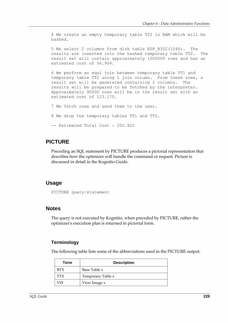
Chapter 6 - Data Administrative Functions
SQL Guide 229
4 We create an empty temporary table TT2 in RAM which will be
hashed.
5 We select 2 columns from disk table EDP_BIG2(1044). The
results are inserted into the hashed temporary table TT2. The
result set will contain approximately 1000000 rows and has an
estimated cost of 56.904.
6 We perform an equi join between temporary table TT1 and
temporary table TT2 using 1 join column. From these rows, a
result set will be generated containing 2 columns. The
results will be prepared to be fetched by the interpreter.
Approximately 90000 rows will be in the result set with an
estimated cost of 123.170.
7 We fetch rows and send them to the user.
8 We drop the temporary tables TT1 and TT2.
-- Estimated Total Cost : 205.822
PICTURE
Preceding an SQL statement by PICTURE produces a pictorial representation that describes how the optimizer will handle the command or request. Picture is discussed in detail in the Kognitio Guide.
Usage
PICTURE query-statement
Notes
The query is not executed by Kognitio, when preceded by PICTURE, rather the optimizer's execution plan is returned in pictorial form.
Terminology
The following table lists some of the abbreviations used in the PICTURE output.
Term Description
BTX Base Table x
TTX Temporary Table x
VIX View Image x
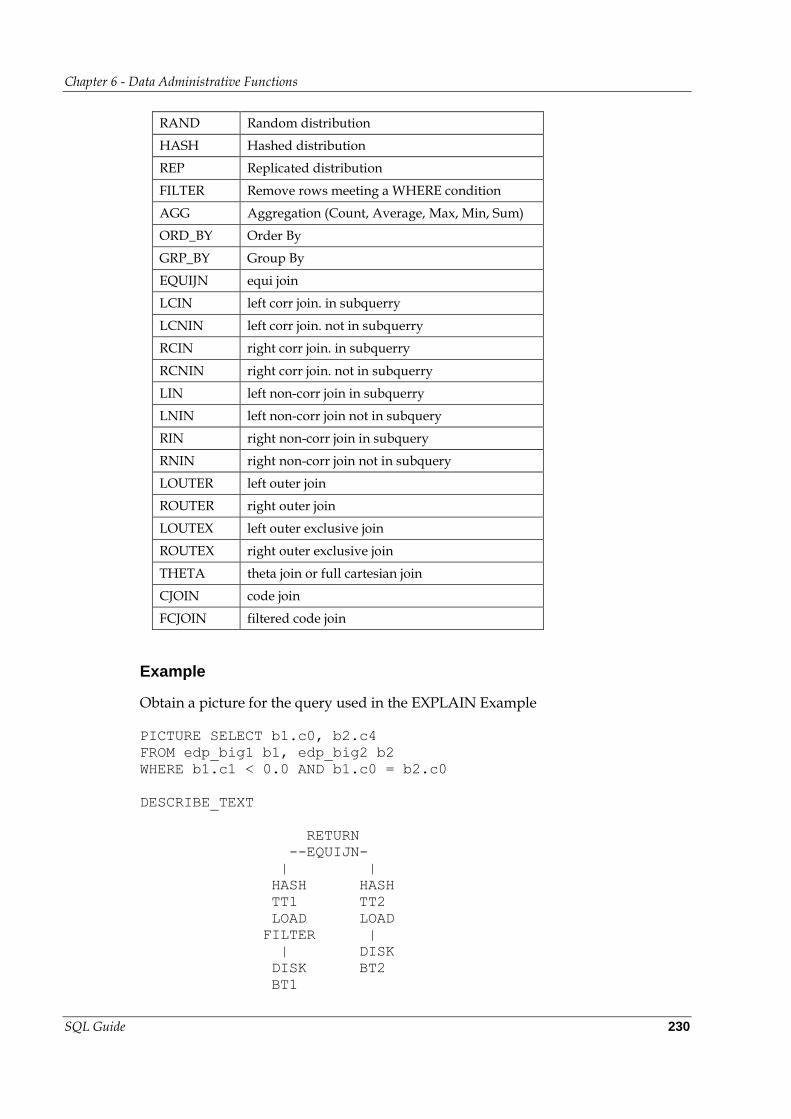
Chapter 6 - Data Administrative Functions
SQL Guide 230
RAND Random distribution
HASH Hashed distribution
REP Replicated distribution
FILTER Remove rows meeting a WHERE condition
AGG Aggregation (Count, Average, Max, Min, Sum)
ORD_BY Order By
GRP_BY Group By
EQUIJN equi join
LCIN left corr join. in subquerry
LCNIN left corr join. not in subquerry
RCIN right corr join. in subquerry
RCNIN right corr join. not in subquerry
LIN left non-corr join in subquerry
LNIN left non-corr join not in subquery
RIN right non-corr join in subquery
RNIN right non-corr join not in subquery
LOUTER left outer join
ROUTER right outer join
LOUTEX left outer exclusive join
ROUTEX right outer exclusive join
THETA theta join or full cartesian join
CJOIN code join
FCJOIN filtered code join
Example
Obtain a picture for the query used in the EXPLAIN Example
PICTURE SELECT b1.c0, b2.c4
FROM edp_big1 b1, edp_big2 b2
WHERE b1.c1 < 0.0 AND b1.c0 = b2.c0
DESCRIBE_TEXT
RETURN
--EQUIJN-
| |
HASH HASH
TT1 TT2
LOAD LOAD
FILTER |
| DISK
DISK BT2
BT1
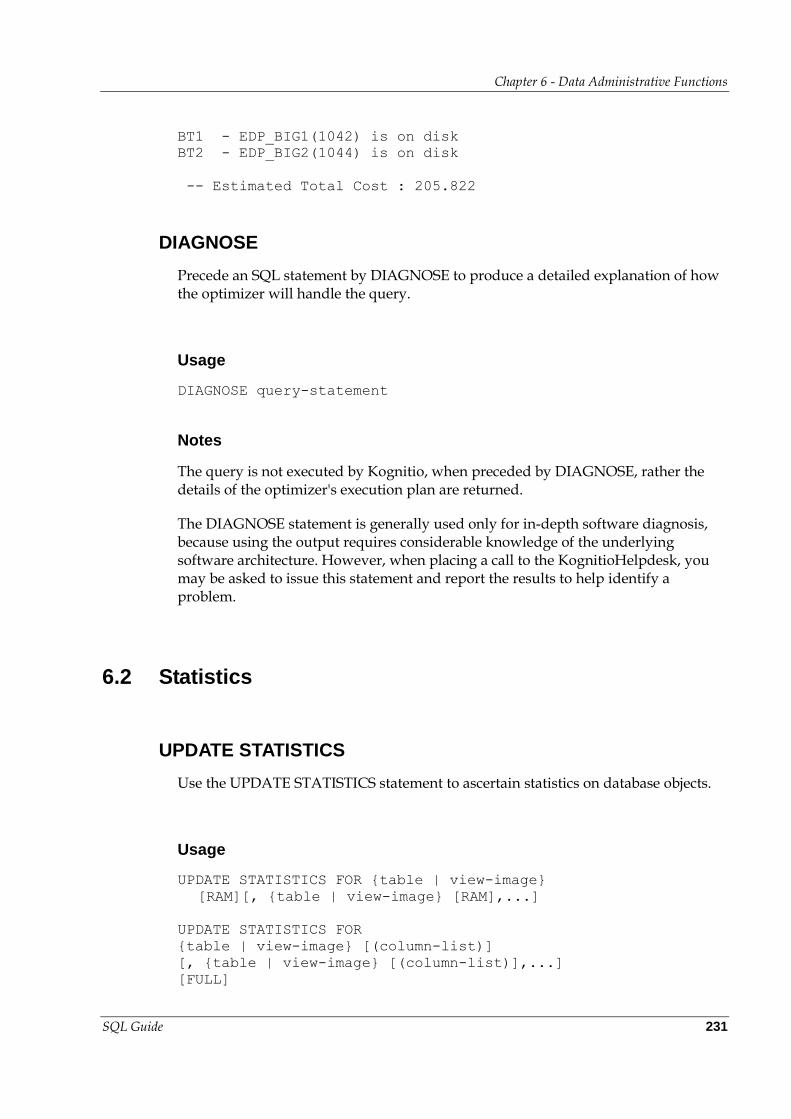
Chapter 6 - Data Administrative Functions
SQL Guide 231
BT1 - EDP_BIG1(1042) is on disk
BT2 - EDP_BIG2(1044) is on disk
-- Estimated Total Cost : 205.822
DIAGNOSE
Precede an SQL statement by DIAGNOSE to produce a detailed explanation of how the optimizer will handle the query.
Usage
DIAGNOSE query-statement
Notes
The query is not executed by Kognitio, when preceded by DIAGNOSE, rather the details of the optimizer's execution plan are returned.
The DIAGNOSE statement is generally used only for in-depth software diagnosis, because using the output requires considerable knowledge of the underlying software architecture. However, when placing a call to the KognitioHelpdesk, you may be asked to issue this statement and report the results to help identify a problem.
6.2 Statistics
UPDATE STATISTICS
Use the UPDATE STATISTICS statement to ascertain statistics on database objects.
Usage
UPDATE STATISTICS FOR {table | view-image}
[RAM][, {table | view-image} [RAM],...]
UPDATE STATISTICS FOR
{table | view-image} [(column-list)]
[, {table | view-image} [(column-list)],...]
[FULL]
Chapter 6 - Data Administrative Functions
SQL Guide 232
Notes
Using UPDATE STATISTICS FOR {table | view-image} RAM records current and historical (i.e. deleted records since last CREATE TABLE IMAGE) size for the table.
If no column-list is supplied, all columns are assumed.
Using UPDATE STATISTICS FOR {table | view-image} records cardinality and the selectivity of the column. If the cardinality hasn’t changed since the statistics were last collected, then they are not refreshed—and the command will complete faster than expected. Using the FULL keyword forces statistics to be updated, even if the cardinality has not changed.
Selectivity can only be updated for columns with a RAM image. If the table is not in RAM than only the cardinality will be updated.
The compiler/optimizer can make better decisions about how to execute a query, if the statistics about the table(s) involved are up to date. If the tables referenced in a query have changed significantly since statistics were last collected, give an UPDATE STATISTICS command before running the query. Changes are reflected in the results you obtain from EXPLAIN and PICTURE.
Normally, UPDATE STATISTICS FOR table determines cardinality and selectivity using a statistically sound sampling mechanism. However, if there is any reason to believe that the statistics might not be sufficiently accurate, use the command UPDATE STATISTICS FOR table FULL. This results in exact statistics being returned, but can take a long time particularly for tables with a large number of rows and columns. (This may be useful in benchmarking and tuning.)
For information on using statistics, see the Kognitio Guide.
Example
Collect statistics on different tables and columns in the tables.
UPDATE STATISTICS FOR part RAM
UPDATE STATISTICS FOR part RAM, supplier RAM, partsupp RAM
UPDATE STATISTICS FOR ordertab(o_orderkey, o_custkey)
UPDATE STATISTICS FOR partsupp(ps_partkey, ps_suppkey),
part(p_partkey), customer(c_custkey)
Chapter 6 - Data Administrative Functions
SQL Guide 233
DROP STATISTICS
Use the DROP STATISTICS statement to remove all statistical information for a particular object. See the Kognitio Guide, for information on using statistics.
Usage
DROP STATISTICS FOR object-name
INSERT STATISTICS
Use the INSERT STATISTICS statement to change or set statistical information. See the Kognitio Guide, for information on using statistics.
Usage
INSERT STATISTICS FOR object-name
[SET CARDINALITY value]
[(column-name = value[, column-name = value],...
|ALL = value)]
Where
object-name is the name of the table/view image whose statistics are being set.
CARDINALITY value specifies the required value for the number of rows.
column-name is the name of a column in the target object.
value specifies the value of the selectivity of the column or the NULL keyword.
Notes
This command lets you manipulate statistics relating to data tables and view images manually. This means you can specify the statistics required to update the relevant system tables in SQL — without requiring a global lock.
Normally statistics are only inserted to check what effects differing amounts of data might have on a query plan, without the need to load extra data.
Example
Insert statistics on various tables.
Chapter 6 - Data Administrative Functions
SQL Guide 234
INSERT STATISTICS FOR sampletable
SET CARDINALITY 100(col1 = 45, col2 = NULL, col3 = 76)
INSERT STATISTICS FOR benchmark
SET CARDINALITY 100000
INSERT STATISTICS FOR test_vi
(COL1 = 12, COL2 = 10000, COL3 = NULL)
INSERT STATISTICS FOR production
SET CARDINALITY NULL(ALL = NULL)
6.3 NFS Import and Export
IMPORT
Use the IMPORT statement to transfer data in WCB (Kognitio Compatible Binary) format, into a table on Kognitio. Note that if the WCB file contains a valid table definition, then the table is created automatically, otherwise it must already exist.
Note: NFS import/export is a legacy feature which only supports Kogitio Compatible Binary format; it is slower than direct import/export and doesn't support parallel import/export.
Usage
IMPORT FROM server FILE file-name INTO table
Notes
Before using the IMPORT statement, you must ensure that the Import/Export tables (IPE_FILE, IPE_FILE_FORMAT, IPE_FIELD,IPE_REM_USER, IPE_REM_SERVER) have been set up correctly to make the data transfer.
The IMPORT command performs the following tasks.
It reads the Import/Export tables for the mapping between source file and destination table.
It verifies that the import file definition matches the table definition.
It writes binary records from the import file as rows in the table.
Use the IMPORT statement to transfer files in WCB format, but note that no format conversion or integrity checking can be performed.
Chapter 6 - Data Administrative Functions
SQL Guide 235
It is possible for the create statement generated from the WCB file to contain duplicate column names. In this case the automatic attempt to create the table fails.
It is possible for the create statement generated from the WCB file to contain derived column names that have to be included in quotes in subsequent SQL statements, e.g. "S.ID", "COUNT(*)", etc.
IMPORT can also been performed using the WXDataport utility, which is discussed in the Kognitio Guide.
Example
Import data into the SAVERS table from the file on the network file server (represented by the entry for ‘NUADA’ in IPE_REM_SERVER) that is referenced by the SAVEINFO reference in IPE_FILE.
IMPORT FROM nuada FILE saveinfo INTO savers
EXPORT
Use the EXPORT statement to transfer data, in WCB (Kognitio Compatible Binary)
format, from an existing table, view, or a select-statement. As well as the data, the WCB file will contain a definition of the source data so, if necessary, an attempt can be made to automatically create a table when the file is re-imported on to Kognitio.
Note: NFS import/export is a legacy feature which only supports Kognitio Compatible Binary format; it is slower than direct import/export and doesn't support parallel import/export.
Usage
EXPORT TO server FILE file-name FROM select-statement
Notes
Before using the EXPORT statement, you must first ensure that the Import/Export tables (IPE_FILE, IPE_FILE_FORMAT, IPE_FIELD, IPE_REM_USER, IPE_REM_SERVER) are set up correctly to make the data transfer.
The Export command performs the following tasks.
It reads the Import/Export tables for the mapping between file and table(s)/view(s).
It selects rows from the export table(s)/view(s) to transfer as binary records.
Chapter 6 - Data Administrative Functions
SQL Guide 236
Any SELECT may be used after the FROM, including joins and aggregates.
It is possible for the default create statement generated from the WCB file to contain duplicate column names. In this case any automatic attempt to create the table will fail. To avoid this use column aliases in the SELECT statement.
It is possible for the default create statement generated from the WCB file to contain derived column names that have to be included in quotes in subsequent SQL statements, e.g. "S.ID", "COUNT(*)", etc. To avoid this use column aliases in the SELECT statement.
Export can also been performed using the WXDataport utility, which is discussed in the Kognitio Guide.
Example
Export selected columns (C_CUSTKEY, C_NAME, C_ADDRESS AND C_ACCTBAL) from the CUSTOMER table into the file on the network file server (represented by the entry for ‘NUADA’ in IPE_REM_SERVER) that is referenced by the CUSTINFO reference in IPE_FILE.
EXPORT TO nuada FILE custinfo FROM
SELECT c_custkey, c_name, c_address, c_acctbal
FROM customer
6.4 Compressed Data Maps
The Kognitio implementation includes four Compressed Data Map statements
UPDATE STATISTICS FOR COMPRESSED DATA MAP
CREATE COMPRESSED DATA MAP
DROP COMPRESSED DATA MAP
DROP STATISTICS FOR COMPRESSED DATA MAP.
For more information about using Compressed Data Maps, see the Kognitio Guide.
UPDATE STATISTICS FOR COMPRESSED DATA MAP
Use the UPDATE STATISTICS FOR COMPRESSED DATA MAP statement to establish statistics on a particular column of a table prior to creating a compressed data map. This gathers the statistics required to build a compressed data map, and stores them in the IPE_COMP system table. For more information about Compressed Data Maps, see the Kognitio Guide.
Chapter 6 - Data Administrative Functions
SQL Guide 237
Usage
UPDATE STATISTICS FOR COMPRESSED DATA MAP
ON table(column [PRECISION precision],...)
Notes
The limit on the number of columns that you can specify using an UPDATE STATISTICS FOR COMPRESSED DATA MAP command is six.
Use precision to specify the number of bits that should be used from each exact numeric data type. This lets you perform the type of operation shown in Example 3, which can make data suitable for access via a compressed data map.
Before using the UPDATE STATISTICS FOR COMPRESSED DATA MAP command, you require SELECT, INSERT and UPDATE access to the system table IPE_COMP.
Example 1 – Update Compressed Data Map Statistics on One Column
Update compressed data map statistics on the o_ordertab column of the ORDERTAB table.
UPDATE STATISTICS FOR COMPRESSED DATA MAP
ON ordertab(o_orderdate)
Example 2 – Update Compressed Data Map Statistics on Multiple Columns
Update compressed data map statistics on the ps_partkey and ps_suppkey columns of the PARTSUPP table.
UPDATE STATISTICS FOR COMPRESSED DATA MAP
ON partsupp(ps_partkey, ps_suppkey)
Example 3 – Update Compressed Data Map Statistics and Precision
Update compressed data map statistics on six columns from the PART table. Set the precision for two of the three exact numeric columns.
UPDATE STATISTICS FOR COMPRESSED DATA MAP
ON part(p_partkey PRECISION 12,
p_name,
p_type,
p_mfgr,
p_size,
p_retailprice PRECISION 17)
Chapter 6 - Data Administrative Functions
SQL Guide 238
CREATE COMPRESSED DATA MAP
Use the CREATE COMPRESSED DATA MAP statement to create a compressed data map for a specified table and (optionally) a column-list. Before using this command, you must have run the UPDATE STATISTICS FOR COMPRESSED DATA MAP command.
Usage
CREATE COMPRESSED DATA MAP ON table[(column-list)]
Notes
Specifying multiple columns doesn’t indicate composite data maps; each data map created is independent. Specifying multiple columns simply means that multiple data maps are created with a single table scan.
The UPDATE STATISTICS FOR COMPRESSED DATA MAP command specifies which columns to collect statistics for. Once statistics are gathered, running a CREATE COMPRESSED DATA MAP without specifying any columns builds the compressed data maps for the columns with statistics. If, at a later date, you run UPDATE STATISTICS FOR COMPRESSED DATA MAP on a different column and then run CREATE COMPRESSED DATA MAP, Kognitio just builds the data map for that column. However, if there is nothing new to build you get an error.
Compressed data maps reside in RAM on DiskStore nodes. They can be very efficient when used on columns where the data is clustered. In clustered data records close together on disk, are likely to have the same column values.
Any compressed data maps established prior to a machine shutdown are reinstated if a CREATE IMAGE command is issued.
If a CREATE SYSTEM IMAGE command is issued, any compressed data maps are dropped.
Data maps are maintained if data is added to or deleted from the associated table.
Example 1 – Create a Compressed Data Map on a Table
Once statistics have been gathered (using the UPDATE STATISTICS FOR COMPRESSED DATA MAP command), running a CREATE COMPRESSED DATA MAP command on a table without specifying any columns builds the compressed data maps for all columns with compressed data map statistics.
CREATE COMPRESSED DATA MAP ON ordertab
Chapter 6 - Data Administrative Functions
SQL Guide 239
Example 2 – Create a Compressed Data Map for Specific Columns
After gathering statistics (using the UPDATE STATISTICS FOR COMPRESSED DATA MAP command), create compressed data maps for specific columns on a table.
To create the compressed data map on the o_orderdate column of the ORDERTAB table, run
CREATE COMPRESSED DATA MAP ON ordertab(o_orderdate)
To create the compressed data maps on the ps_partkey and ps_suppkey columns of the PARTSUPP table, run
CREATE COMPRESSED DATA MAP ON partsupp(ps_partkey, ps_suppkey)
DROP COMPRESSED DATA MAP
Use the DROP COMPRESSED DATA MAP statement to drop any compressed data map created previously.
For more information on setting up and using Compressed Data Maps, see the Kognitio Guide.
Usage
DROP COMPRESSED DATA MAP ON table[(column-list)]
If no columns are named, then all compressed data maps for the table are dropped.
Example 1 – Drop the Compressed Data Map for a Table
To drop all compressed data maps for the ORDERTAB table, use
DROP COMPRESSED DATA MAP ON ordertab
Example 2 – Drop the Compressed Data Map for Specific Columns
To drop the compressed data map for c_nationkey column of the CUSTOMER table, use
DROP COMPRESSED DATA MAP ON customer(c_nationkey)
Chapter 6 - Data Administrative Functions
SQL Guide 240
DROP STATISTICS FOR COMPRESSED DATA MAP
Use the DROP STATISTICS FOR COMPRESSED DATA MAP statement to drop any previously established statistics on a table. For more information about Compressed Data Maps, see the Kognitio Guide.
Usage
DROP STATISTICS FOR COMPRESSED DATA MAP
ON table[(column-list)]
Notes
To use the DROP STATISTICS command, you require SELECT, DELETE and UPDATE access to the table IPE_COMP.
This command deletes the compressed data map statistics for the named columns. If you don’t specify any columns, the compressed data map statistics for all columns in the table are dropped.
Note that you cannot successfully run the DROP STATISTICS FOR COMPRESSED DATA MAP command if a compressed data map exists on any of the columns in the list (or table); you must drop any compressed data maps before dropping the compressed data map statistics.
Example 1 – Drop the Compressed Data Map and All Compressed Data Map Statistics for a Table
To drop all statistics previously collected on the CUSTOMER table.
DROP COMPRESS DATA MAP ON customer
DROP STATISTICS FOR COMPRESSED DATA MAP ON customer
Example 2 – Drop all Compressed Data Map Statistics for a Specific Column in a Table
To drop compressed data map statistics previously collected on the O_ORDERDATE column of the ORDERTAB table, use
DROP STATISTICS FOR COMPRESSED DATA MAP ON
ordertab(o_orderdate)
Chapter 6 - Data Administrative Functions
SQL Guide 241
6.5 Kognitio Administrative Functions
Kognitio has three main groups of administration commands, all of which are extensions to SQL. The first group covers commands required to
Obtain a global session (LOCK SYSTEM command)
Set up a lock on a table that lasts for the duration of the current transaction lock (LOCK TABLE command)
Restore data previously held in RAM, for example, after a restart (CREATE IMAGE command)
Perform a RECLAIM to maximize available disk space.
The LOCK SYSTEM, CREATE IMAGE and RECLAIM commands are discussed in this section.
The second group of commands is for creating security classes (CREATE SEC_CLASS, ALTER SEC_CLASS) and manipulating query queues (CREATE QUEUE, ALTER QUEUE) – These commands are documented in the Kognitio Guide.
The final group of commands is for initiating a New System, verifying and repairing disk data structures (DISK_REPAIR, DISK_CHECK) and for maintaining disk resources (RECREATE, SPIN) – These are documented in the Kognitio Configuration and Maintenance Manual.
LOCK SYSTEM
Use the LOCK SYSTEM statement to obtain a global session, that is, to prevent access to Kognitio by sessions other than the current one. You can only do this if there are no other connections to Kognitio—if other sessions are running, you receive an error message.
Usage
LOCK SYSTEM
Notes
The LOCK SYSTEM command is normally reserved for the exclusive use of the System Administrator—but this can be changed. (To use the command, you need the CREATE SYSTEM IMAGE privilege, which permits you to lock the system.)
Global sessions are compulsory when updating certain system tables, for example, IPE_USER.
Chapter 6 - Data Administrative Functions
SQL Guide 242
After a user issues a LOCK SYSTEM command and obtains a global session, any attempt to access Kognitio by another session receives the error message
Sessions inhibited
The user who obtains the global session holds it until he/she logs off. That is, they must issue
A DISCONNECT, or
An implicit disconnect by reconnecting to Kognitio.
There is no "unlock" command.
For more information, see the Kognitio Guide.
Example
To obtain a global session in order to initiate a GSR (Global Session Reclaim), use
LOCK SYSTEM
LOCK TABLE
Use the LOCK TABLE statement to set up a lock that lasts for the duration of the current transaction, (that is, up to the next COMMIT or ROLLBACK). To hold the lock for any length of time, you have to be running in Transaction Mode.
Usage
LOCK TABLE table IN {SHARE | EXCLUSIVE} MODE
Notes
The command can be used if you need to perform a complex transaction containing several UPDATE or DELETE queries, and want to make sure that all the objects being manipulated are locked as early as possible within the transaction.
Example
The example shows the effect of using the LOCK TABLE command on two sessions.
Session 1 Session 2
SET MODE TRANSACTION
Chapter 6 - Data Administrative Functions
SQL Guide 243
LOCK TABLE mjbt1 IN EXCLUSIVE MODE
SELECT * FROM mjbt1
Result: LOCK TIMEOUT
COMMIT
SELECT * FROM mjbt1
Result: OK
LOCK TABLE mjbt1 IN SHARE MODE
SELECT * FROM mjbt1
Result: OK
DELETE FROM mjbt1
Result: LOCK TIMEOUT
COMMIT
DELETE FROM mjbt1
Result: OK
If a lock is held for a long time, or a session or query is aborted whilst waiting for locks, then the locks will be dumped to a locks log file for future investigation.
The parameter da_dump_lkti sets how long a lock has to be held for in seconds before triggering the dump; the default period is 10 minutes, to disable the functionality set the parameter to 0.
CREATE SYSTEM IMAGE
Typically, the only time a CREATE [SYSTEM] IMAGE command is required is after a restart. CREATE SYSTEM IMAGE loads the minimal amount into RAM for a working system, and updates the System tables to reflect this. CREATE IMAGE loads RAM with the tables that were resident before the restart, as dictated by the System table contents.
Usage
CREATE [SYSTEM] IMAGE
Notes
On restarting the system, CREATE [SYSTEM] IMAGE attempts to restore Kognitio to a consistent state. This includes recreating any potentially inconsistent RAID parity areas, completing any pending RECLAIM, and rolling back any incomplete transactions.
Chapter 6 - Data Administrative Functions
SQL Guide 244
In all situations, the System tables are loaded into RAM from disk. On receiving a CREATE SYSTEM IMAGE command, all user tables are marked as being on disk and all view images and compressed data maps are dropped. On receiving a CREATE IMAGE command, all table and view images (other than ROTTs) that were present when the system was last up, are reloaded.
For more information, see the Kognitio Guide.
RECLAIM
Use the RECLAIM statement to reclaim disk space currently occupied by records that have been deleted or rolled back in transactions, and so maximize available free disk space. RECLAIM is discussed in the Kognitio Guide.
Usage
RECLAIM [FOR PARTITION {slab_id} ...] TO {NOW | BEGIN}
RECLAIM SYSTEM TABLE ROWS
Notes
Kognitio also provides an automated background repackaging mechanism as an alternative to the RECLAIM command; see the Kognitio Guide for more details.
In the first form of the command individual slabs might be specified if there is only a small daily reclaim window available meaning a different set of slabs have to be reclaimed each night; alternatively you may wish to target an individual slab because you have deleted a significant number of records from it, for example, you may have deleted old logging records from the logging slab.
Both RECLAIM TO BEGIN and RECLAIM TO NOW run as a Global Session Reclaim (GSR)— the session running the command must have a global lock.
RECLAIM may take several hours to complete, so Kognitiorecommends that you timetable reclaims on a regular basis, and run them overnight or at week-ends.
The sole difference between RECLAIM TO BEGIN and RECLAIM TO NOW is that
RECLAIM TO BEGIN only reclaims information that can never be used again, for example, "delete" and "transaction complete" markers from completed transactions, and rolled-back rows. For this reason, it is rarely used.
Chapter 6 - Data Administrative Functions
SQL Guide 245
RECLAIM TO NOW reclaims all non-current information from completed transactions, for example, everything that "RECLAIM TO BEGIN" would reclaim, plus deleted/updated rows and dropped tables. This form of RECLAIM is the one normally used.
The second form of the command has the effect of deleting all the old system table rows which do not have a corresponding entry in IPE_ALLTABLE; this is similar to the effect of running a CREATE [SYSTEM] IMAGE command but does not require the user images to be reloaded in to RAM. Reclaim privilege is required to run the command. Kognitio recommend using the LOCK SYSTEM command to obtain a global session prior to running the command to prevent potential locking issues with concurrent sessions.
For more information on RECLAIM, see the Kognitio Guide.
Example 1 – Global Session Reclaim
Perform a Global Session Reclaim (GSR)
LOCK SYSTEM
RECLAIM TO NOW
Remember that a CREATE IMAGE command automatically obtains a global lock, so the following would run as a GSR.
CREATE IMAGE
RECLAIM TO NOW
Example 2 – Global Session Reclaim of Specific Slabs
Perform a Global Session Reclaim (GSR) of specific slabs
LOCK SYSTEM
RECLAIM FOR PARTITION 3 4 TO NOW

Kognitio SQL Guide 247
7
Using Date-times and Intervals The date-time data types include: DATE, TIME, TIMESTAMP and INTERVAL, and the fields include: YEAR, MONTH, DAY, HOUR, MINUTE and SECOND. See Intervals, Dates and Times on page 5 for more information on definitions for these data types and fields.
This section explains how to use date-time data types. It includes the following topics.
Creating Tables with Date-times and Interval Columns.
Inserting Dates, Times and Intervals.
Adding and Subtracting Date-times and Intervals.
Aggregation with Date-times and Intervals.
The following functions are also useful when dealing with date-times:
EXTRACT.
DAYOFWEEK.
PACKDATE.
CURRENT_DATE, CURRENT_TIME, CURRENT_TIMESTAMP.
Creating Tables with Date-time, Interval and Timestamp Columns
In table definitions, Date and Time columns are simply entered as DATE and TIME. TIMESTAMPS may include a precision.
Example 1 – Creating a Table with Interval Columns
Create a table to hold details about the length of journeys in days, hours, minutes and seconds.
CREATE TABLE journeys(
journey CHAR(8),
Chapter 7- Using Date-times and Intervals
SQL Guide 248
precise_time_tosecond INTERVAL DAY(3) TO SECOND)
Example 2 – CREATE TABLE with Date, Time, and Timestamp Without Precision
The ORDERTAB table has DATE, TIME and TIMESTAMP columns. No precision set for the TIMESTAMP, so the fractional precision for the SECOND field is 6, the default value.
CREATE TABLE ordertab(
o_orderkey INT NOT NULL,
o_custkey INT,
o_orderstatus CHAR(1),
o_totalprice DECIMAL(12, 2),
o_orderdate DATE,
o_ordertime TIME,
o_orderpriority CHAR(15),
o_deliverytime TIMESTAMP,
PRIMARY KEY(o_orderkey))
Example 3 – CREATE TABLE with Date, Time, and Timestamp with Precision Set
This table definition has a TIMESTAMP field where the precision is set to 0, which means there are no sub seconds.
CREATE TABLE ipe_table(
schema_id INTEGER NOT NULL,
name CHAR(32) NOT NULL,
id INTEGER NOT NULL,
owner INTEGER NOT NULL,
type CHAR(1) NOT NULL,
create_time TIMESTAMP(0),
PRIMARY KEY(id),
UNIQUE(name, schema_id),
FOREIGN KEY(schema_id) REFERENCES ipe_schema)
Inserting Date, Times and Intervals
Intervals
When you enter an INTERVAL into a column, or SELECT or manipulate INTERVAL values, you may use INTERVAL literals, INTERVAL calculations or CAST them from another data type.
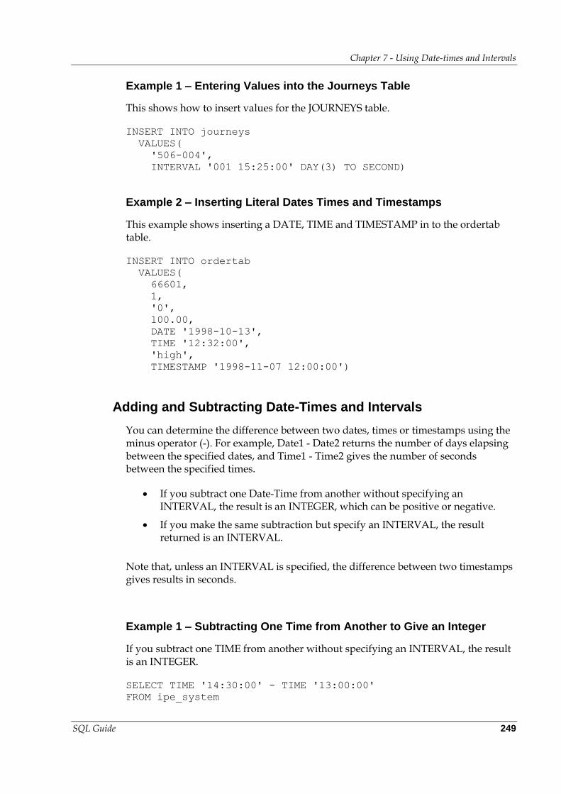
Chapter 7 - Using Date-times and Intervals
SQL Guide 249
Example 1 – Entering Values into the Journeys Table
This shows how to insert values for the JOURNEYS table.
INSERT INTO journeys
VALUES(
'506-004',
INTERVAL '001 15:25:00' DAY(3) TO SECOND)
Example 2 – Inserting Literal Dates Times and Timestamps
This example shows inserting a DATE, TIME and TIMESTAMP in to the ordertab table.
INSERT INTO ordertab
VALUES(
66601,
1,
'0',
100.00,
DATE '1998-10-13',
TIME '12:32:00',
'high',
TIMESTAMP '1998-11-07 12:00:00')
Adding and Subtracting Date-Times and Intervals
You can determine the difference between two dates, times or timestamps using the minus operator (-). For example, Date1 - Date2 returns the number of days elapsing between the specified dates, and Time1 - Time2 gives the number of seconds between the specified times.
If you subtract one Date-Time from another without specifying an INTERVAL, the result is an INTEGER, which can be positive or negative.
If you make the same subtraction but specify an INTERVAL, the result returned is an INTERVAL.
Note that, unless an INTERVAL is specified, the difference between two timestamps gives results in seconds.
Example 1 – Subtracting One Time from Another to Give an Integer
If you subtract one TIME from another without specifying an INTERVAL, the result is an INTEGER.
SELECT TIME '14:30:00' - TIME '13:00:00'
FROM ipe_system
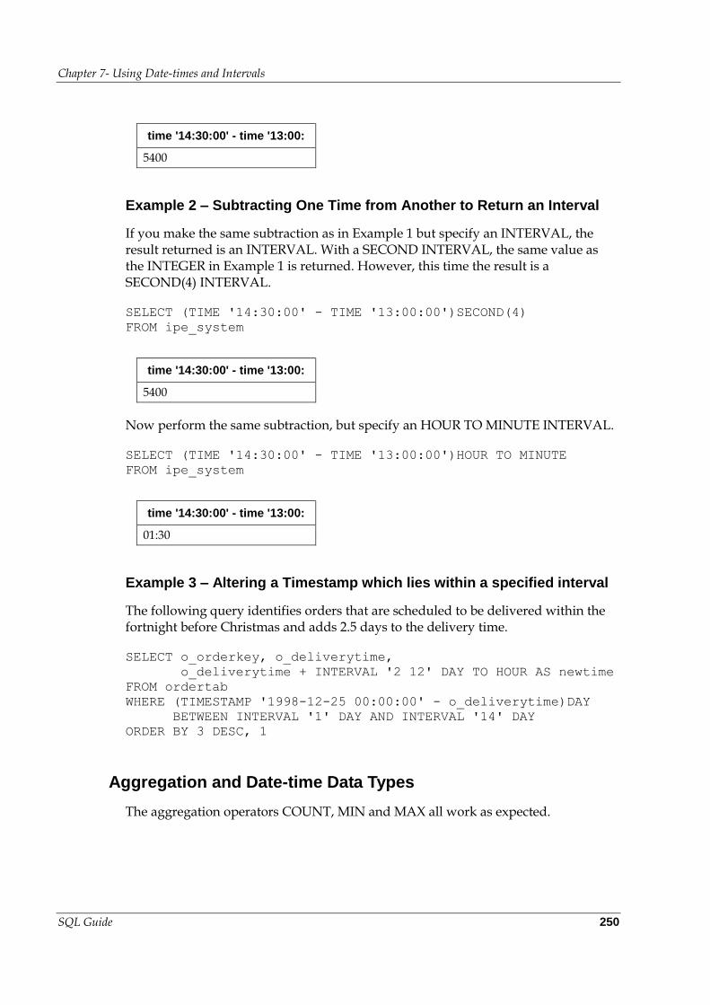
Chapter 7- Using Date-times and Intervals
SQL Guide 250
time '14:30:00' - time '13:00:
5400
Example 2 – Subtracting One Time from Another to Return an Interval
If you make the same subtraction as in Example 1 but specify an INTERVAL, the result returned is an INTERVAL. With a SECOND INTERVAL, the same value as the INTEGER in Example 1 is returned. However, this time the result is a SECOND(4) INTERVAL.
SELECT (TIME '14:30:00' - TIME '13:00:00')SECOND(4)
FROM ipe_system
time '14:30:00' - time '13:00:
5400
Now perform the same subtraction, but specify an HOUR TO MINUTE INTERVAL.
SELECT (TIME '14:30:00' - TIME '13:00:00')HOUR TO MINUTE
FROM ipe_system
time '14:30:00' - time '13:00:
01:30
Example 3 – Altering a Timestamp which lies within a specified interval
The following query identifies orders that are scheduled to be delivered within the fortnight before Christmas and adds 2.5 days to the delivery time.
SELECT o_orderkey, o_deliverytime,
o_deliverytime + INTERVAL '2 12' DAY TO HOUR AS newtime
FROM ordertab
WHERE (TIMESTAMP '1998-12-25 00:00:00' - o_deliverytime)DAY
BETWEEN INTERVAL '1' DAY AND INTERVAL '14' DAY
ORDER BY 3 DESC, 1
Aggregation and Date-time Data Types
The aggregation operators COUNT, MIN and MAX all work as expected.
Chapter 7 - Using Date-times and Intervals
SQL Guide 251
Example – Aggregation with Date-times
Find the earliest order placed by each customer in the ordertab table.
SELECT o_custkey, MIN(o_orderdate)
FROM ordertab
GROUP BY 1
ORDER BY 1

Kognitio SQL Guide 253
8
Using National Character Sets
You can use Kognitio to store national characters based on the syntax extensions to SQL:1999, which use Unicode and ISO standards. Using these extensions, you can store Latin and national characters, including Kanji.
Overview
The best known and most widely used character encoding standard is ASCII, which is based on 7-bit byte character strings and has enough characters to encode English text, but no other major written languages.
ISO has standardized several 8-bit extensions of ASCII for various groups of Latin-based writing systems. Latin-1 supports Western European languages and is widely used. Unicode is the problem-free way to handle written languages that are not in the Latin-1 list.
The Unicode Standard
The Unicode Standard is an effort to encode all the world’s characters in one standard. Unicode encodes over 100,000 characters The Unicode Standard specifies a numeric value and a name for each of its characters. In this respect, it is similar to other character encoding standards such as ASCII.
The range of integers used to code the characters is called the code space. A particular integer in this range is called a code point. When a character is mapped or assigned to a particular code point in the code space, it is referred to as a coded character.
Chapter 8 - Using National Character Sets
SQL Guide 254
The Unicode Standard defines three encoding forms that allow the same data to be stored and transmitted in a byte, double-byte or quad-byte oriented format (that is, in 8-, 16-, or 32-bits per code unit). All three encoding forms encode the same common characters and can be efficiently transformed into one another without data loss.
The three encoding forms are:
Name Variable Width Description
UTF-8 Yes Stores each code point as a single 8-bit unit (the ASCII characters), or as two, three or four 8-bit sequences.
UTF-16 Yes Stores each code point using either a single 16-bit unit or as a two 16-bit units.
UTF-32 No Stores each code point as a 32-bit unit.
All three encoding forms need at most 4 bytes of data for each character.
Note: UCS-2 (2-byte Universal Character Set) is a similar yet older character encoding that was superseded by UTF-16 in Unicode version 2.0, though it still remains in use. The UCS-2 encoding form is identical to that of UTF-16, except that it does not support surrogate pairs and as a consequence it is a fixed-length encoding that always encodes characters into a single 16-bit value.
Kognitio Character Set Specification
The full syntax for specifying a CHAR or VARCHAR field is:
CHAR|VARCHAR (length) [CHARACTER SET character-set]
The character-set specified here is used for storage and conversion. For storage, different character sets take different amounts of space. For example:
Name Bytes per character Full Unicode Variable Width
LATIN1 1 No No
UCS2 2 No No
UTF8 1-4 Yes Yes
UTF16 2 or 4 Yes Yes
UTF32 4 Yes No
The character sets recognised by Kognitio are defined in the system tables IPE_CHARACTER_SET and IPE_CHARSET_TRANSLATION; custom 1 byte character sets can be added.
If the character set for a field is not specified, then the system default character set is used. When creating tables, the schema default character set overrides the system default. The system default character set is initially set to LATIN1.
Chapter 8 - Using National Character Sets
SQL Guide 255
Defaults are set using the following SQL syntax:
CREATE SCHEMA schema DEFAULT CHARACTER SET character-set
ALTER SCHEMA schema SET DEFAULT CHARACTER SET TO character-set
ALTER SYSTEM SET DEFAULT CHARACTER SET TO character-set
CHAR fields can only use fixed width character sets, whereas VARCHAR fields can use either fixed or variable width character sets. For this reason you cannot use a variable width character set as the default character set for a schema.
Normal character operations all work as expected, with automatic conversion of character sets being performed by Kognitio when required.
Notes: the automatic conversion of character sets can result in a performance penalty if, for example, strings have to be converted from a single byte representation to a four byte representation.
At present the upper and lower case functions consider Unicode, however the length of strings cannot change (this is the simplest form of conversion), so, for example, LOWER('Δ') will result in 'δ', but UPPER('ß') will not result in 'SS'.
The character set encoding for a session is determined by the client application and ODBC which will covert if necessary for the server. Kognitio does not support multiple character sets in the same SQL statement.
String Comparison
String comparison and sorting is performed using the UCS_BASIC collation order. Where a character offset of length is used, this will normally be in characters rather than bytes.
String Length
The CHAR_LENGTH function defaults to returning the string length as the number of characters, but, if required, it can return the number of bytes; there is also a function, OCTET_LENGTH which returns the string length as the number of bytes:
CHAR_LENGTH(string [USING OCTETS | CHARACTERS])
OCTET_LENGTH(string)
Chapter 8 - Using National Character Sets
SQL Guide 256
Entering Unicode
Identifiers can be entered in Unicode and do not need quoting if they are in the regular identifier form specified by SQL (i.e. a letter followed by a sequence of letters, numbers, non-spacing marks, spacing-combining marks, connector punctuation or formatting codes).
For characters not in the session’s character set, there is a Unicode delimited form which allows any Unicode character to be specified using its code point escaped by backslash or another escape character.
The following three string literals are equivalent:
'Pólya'
U&'P\00F3lya'
U&'P/00F3lya' UESCAPE '/'
The following four identifiers are equivalent; the first two are equivalent because identifiers are case insensitive.
Erdős
ERDŐS
U&"ERD\0150S"
U&"ERD/0150S" UESCAPE '/'
Altering a Column's Character Set Specification
It is possible to change the specification of a string column using:
ALTER TABLE table
ALTER COLUMN column
ALTER TYPE TO CHAR | VARCHAR(length)
CHARACTER SET character-set
This will also cause the underlying data in the columns to be changed to the new character set.
Alternatively, you can inform Kognitio that you want to change the specification of a column but not alter the underlying data, by using:
ALTER TABLE table
ALTER COLUMN column
ALTER CHARACTER SET TREAT AS character-set
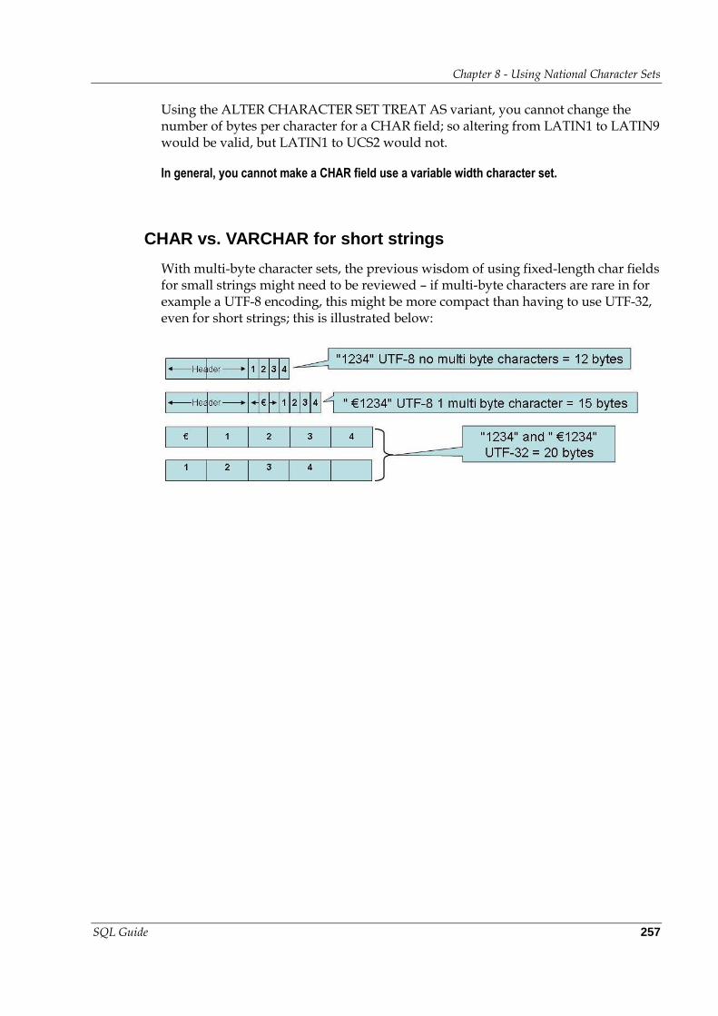
Chapter 8 - Using National Character Sets
SQL Guide 257
Using the ALTER CHARACTER SET TREAT AS variant, you cannot change the number of bytes per character for a CHAR field; so altering from LATIN1 to LATIN9 would be valid, but LATIN1 to UCS2 would not.
In general, you cannot make a CHAR field use a variable width character set.
CHAR vs. VARCHAR for short strings
With multi-byte character sets, the previous wisdom of using fixed-length char fields for small strings might need to be reviewed – if multi-byte characters are rare in for example a UTF-8 encoding, this might be more compact than having to use UTF-32, even for short strings; this is illustrated below:

Kognitio SQL Guide 259
9
Plugin Functions
Plugin modules allow users to write their own C functions and call them from within Kognitio SQL SELECT statements. For an overview of the plugin mechanism and description of the basic procedures for developing and using plugin modules see the Kognitio Guide. This chapter describes the plugin functions that have been developed by Kognitio and are provided as part of the standard Kognitio release.
ADD_MONTHS
ADD_MONTHS adds a number of months to a date.
Module
compatibility
Usage
ADD_MONTHS(date, months)
Notes
If months is negative, the value is subtracted from date.
Non-integer values of months will be truncated.
Chapter 9 - Plugin Functions
SQL Guide 260
Example
This example shows how old someone currently is and also how old they will be in 6 months time.
SELECT name,
AGE(dob) Age_Now,
AGE(dob, ADD_MONTHS(SYSDATE, 6) Age_In6Months
FROM personnel_records
ORDER BY 2, 3, 1
AGE
The AGE function returns an INT4 containing the age of a person or object at a specified date.
Module
datetime
Usage
AGE(date-of-birth)
AGE(date-of-birth, specific-date)
Notes
The first form of the function calculates the AGE using CURRENT_DATE; the second form can be used to calculate the AGE at any specific date.
The calculation of AGE is not straightforward in standard SQL.
If the specific-date is earlier then the date-of-birth then the AGE returned will be negative.
Example
This example shows how old someone currently is and also how old they will be in two weeks time.
SELECT name,
AGE(dob) Age_Now,
AGE(dob, CURRENT_DATE + INTERVAL '14' DAY) Age_In2weeks
FROM personnel_records
Chapter 9 - Plugin Functions
SQL Guide 261
ORDER BY 2, 3, 1
ANALYSE_STRING
The ANALYSE_STRING function allows the user to obtain information about the composition of a CHAR or VARCHAR.
Module
strings
Usage
ANALYSE_STRING(string)
Notes
The result is an INTEGER where each bit has the following meanings:
Bits Meaning
0 String contains white space
1 String contains control characters
2 String contains punctuation
3 String contains numeric
4 String contains upper case characters
5 String contains lower case characters
6 String contains characters > 127
8 - 15 Lowest ASCII value in string
16 - 23 Highest ASCII value in string
24 - 31 Unused (zero)
Punctuation characters are defined as all printable characters outside the range 0-9, A-Z, a-z and space.
The GETBITS plugin function is useful for splitting up the result.
The function is primarily provided to assist data auditing.
Example 1—Checking telephone numbers only contain digits
The following returns all telephone numbers that do not consist solely of characters
in the range 0-9, (the column is a VARCHAR so we do not have any trailing spaces).
Chapter 9 - Plugin Functions
SQL Guide 262
SELECT home_phone
FROM personnel_records
WHERE GETBITS(ANALYSE_STRING(home_phone), 6, 7) <> 8
ORDER BY 1
Example 2—Checking telephone numbers only contain digits or spaces
If we decide that it is acceptable for there to be embedded spaces in the telephone number, then the SQL of example 1 could be changed to the following:
SELECT home_phone
FROM personnel_records
WHERE GETBITS(ANALYSE_STRING(home_phone), 6, 7) NOT IN (8, 9)
ORDER BY 1
Example 3—Largest single digit in a telephone number
For all telephone numbers that consist solely of characters in the range 0-9, output the highest digit of the number.
SELECT home_phone,
CHR(GETBITS(ANALYSE_STRING(home_phone), 23, 8)) hival
FROM personnel_records
WHERE GETBITS(ANALYSE_STRING(home_phone), 6, 7) = 8
ORDER BY 2, 1
BITCOUNT
BITCOUNT returns the number of bits set in the integer argument
Module
miscfuncs
Usage
BITCOUNT(integer-value)
Notes
The argument is treated as an INT64 so BITCOUNT(-1) = 64, even if -1 is an INT1.
Example
The following counts the number of flags set in column c_flags of the customer table.
Chapter 9 - Plugin Functions
SQL Guide 263
SELECT BITCOUNT(cflags)
FROM customer
CONCAT
CONCAT concatenates the two arguments in to a single string.
Module
compatibility
Usage
CONCAT(str1, str2)
Notes
CONCAT is equivalent to str1 || str2.
Example
Use CONCAT to create a full address including postcode for customers, where the address and postcode run together, but are separated by a comma and space.
SELECT c_name customer,
CONCAT(CONCAT(c_address, ', ’), c_postcode) address
FROM customer
ORDER BY 1
DT_INFO
The DT_INFO function allows the user to obtain information about a specified DATE or TIMESTAMP. The function returns the information in an INT4.
Module
datetime
Usage
DT_INFO(specific-datetime, info-string)
Chapter 9 - Plugin Functions
SQL Guide 264
Notes
info-string is one of the following, DAYOFMONTH, DAYOFYEAR, WEEKOFMONTH, WEEKOFYEAR, MONTHOFYEAR or QUARTEROFYEAR
All calculations assume the year begins on 1st January.
Some of the information could also be obtained using EXTRACT, e.g. DAYOFMONTH.
The info-string is not case sensitive and may have trailing spaces.
The info-string must be enclosed in single quotes.
Example
This example shows the day and week numbers of a persons date of birth.
SELECT name,
DT_INFO(dob, 'DAYOFYEAR') DayNo,
DT_INFO(dob, 'WEEKOFYEAR') WeekNo
FROM personnel_records
ORDER BY 1
EARTH_DISTANCE
EARTH_DISTANCE returns the distance between two points on the earth’s surface.
Module
miscfuncs
Usage
EARTH_DISTANCE(lat1, lon1, lat2, lon2, units, method)
Notes
(lat1, lon1) and (lat2, lon2) are the points on the earth’s surface, specified by latitude (-90 to 90) and longitude (-180 to 180).
method specifies how the distance is calculated:
0 indicates a numerically stable Haversine distance formula and a good value for the earth’s average radius.
Chapter 9 - Plugin Functions
SQL Guide 265
1 indicates a Vincenty inverse formula for ellipsoids and so takes the shape of the earth into account, giving a better estimate at the cost of speed.
units specifies the units for the result - 0 for statute miles, 1 for metres.
A five parameter version of the function will default units to 0.
A four parameter version will default units and method to 0.
Example
The following measures the distance between (1,1) and (2,2) using method 0 and returning the answer in miles.
SELECT EARTH_DISTANCE(1, 1, 2, 2)
FIRST_DAY
FIRST_DAY calculates the date of the first day of the month that the given date is in.
Module
compatibility
Usage
FIRST_DAY(date)
Example
This example shows the date of the beginning of the month containing someone's date of birth.
SELECT name, dob, FIRST_DAY(dob) AS startofmonth
FROM personnel_records
ORDER BY 1
FORMATSTR
FORMATSTR converts and formats its arguments into a VARCHAR under the control of the string control. The control string contains two types of objects: ordinary characters, which are simply copied to the output string, and conversion specifications, each of which causes conversion and copying of the next successive argument to FORMATSTR.
Chapter 9 - Plugin Functions
SQL Guide 266
Module
formatstr
Usage
FORMATSTR(control, arg1, arg2, ...)
Notes
Each conversion specification is introduced by the character # and ended by a conversion character. Between the # and conversion character there may be:
A minus sign, which specifies left adjustment of the converted argument in its field.
A digit string specifying minimum field width. The converted object will be output in a field at least this wide, and wider if necessary. The argument will normally be padded with spaces. The exception to this is if the conversion character is a 'd'; in this case zeroes are used if any leading padding characters are required.
A period, which separates the field width from the next digit string.
A digit string, which specifies the maximum number of characters to be output from a string conversion, or the number of digits to be output for floating point conversions. This value is ignored for other types of conversion.
The conversion characters and their meanings are:
a The byte of output is converted to the corresponding 3-digit decimal ASCII code.
c The low byte of an INTEGER or the first character of a CHAR or VARCHAR is output as an ASCII character.
d A DECIMAL or INTEGER.
f A FLOAT.
H An INTEGER, displayed in upper case hexadecimal.
h An INTEGER, displayed in lower case hexadecimal.
s A CHAR or VARCHAR.
Conversion characters are case sensitive.
If the value to be converted is NULL, then a question mark (?) is output, (padded as necessary).
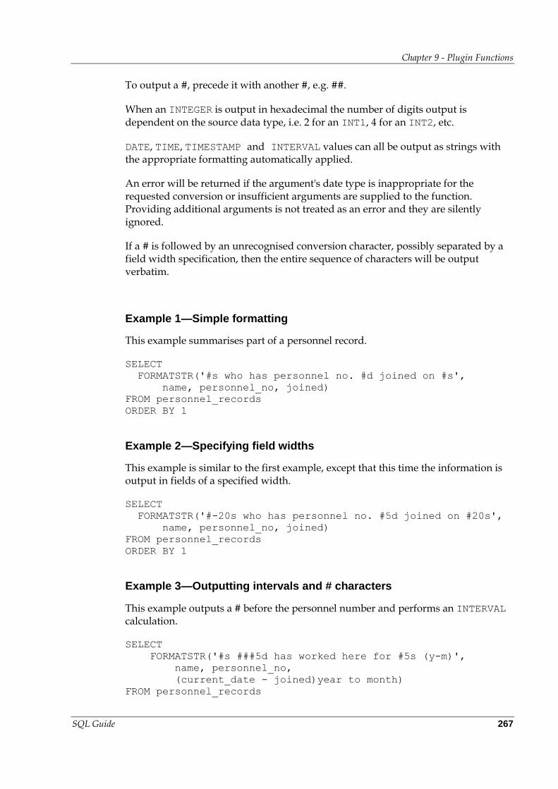
Chapter 9 - Plugin Functions
SQL Guide 267
To output a #, precede it with another #, e.g. ##.
When an INTEGER is output in hexadecimal the number of digits output is dependent on the source data type, i.e. 2 for an INT1, 4 for an INT2, etc.
DATE, TIME, TIMESTAMP and INTERVAL values can all be output as strings with the appropriate formatting automatically applied.
An error will be returned if the argument's date type is inappropriate for the requested conversion or insufficient arguments are supplied to the function. Providing additional arguments is not treated as an error and they are silently ignored.
If a # is followed by an unrecognised conversion character, possibly separated by a field width specification, then the entire sequence of characters will be output verbatim.
Example 1—Simple formatting
This example summarises part of a personnel record.
SELECT
FORMATSTR('#s who has personnel no. #d joined on #s',
name, personnel_no, joined)
FROM personnel_records
ORDER BY 1
Example 2—Specifying field widths
This example is similar to the first example, except that this time the information is output in fields of a specified width.
SELECT
FORMATSTR('#-20s who has personnel no. #5d joined on #20s',
name, personnel_no, joined)
FROM personnel_records
ORDER BY 1
Example 3—Outputting intervals and # characters
This example outputs a # before the personnel number and performs an INTERVAL calculation.
SELECT
FORMATSTR('#s ###5d has worked here for #5s (y-m)',
name, personnel_no,
(current_date - joined)year to month)
FROM personnel_records
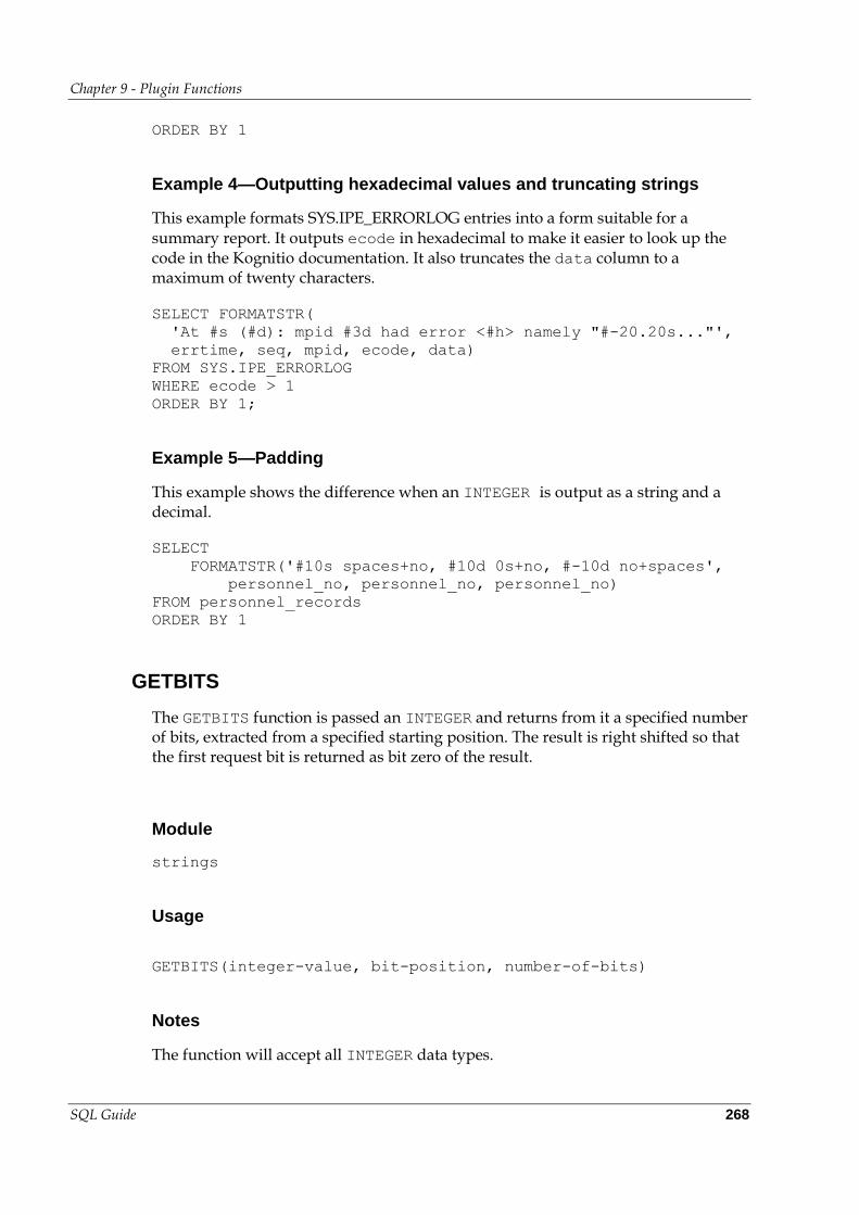
Chapter 9 - Plugin Functions
SQL Guide 268
ORDER BY 1
Example 4—Outputting hexadecimal values and truncating strings
This example formats SYS.IPE_ERRORLOG entries into a form suitable for a summary report. It outputs ecode in hexadecimal to make it easier to look up the code in the Kognitio documentation. It also truncates the data column to a maximum of twenty characters.
SELECT FORMATSTR(
'At #s (#d): mpid #3d had error <#h> namely "#-20.20s..."',
errtime, seq, mpid, ecode, data)
FROM SYS.IPE_ERRORLOG
WHERE ecode > 1
ORDER BY 1;
Example 5—Padding
This example shows the difference when an INTEGER is output as a string and a decimal.
SELECT
FORMATSTR('#10s spaces+no, #10d 0s+no, #-10d no+spaces',
personnel_no, personnel_no, personnel_no)
FROM personnel_records
ORDER BY 1
GETBITS
The GETBITS function is passed an INTEGER and returns from it a specified number of bits, extracted from a specified starting position. The result is right shifted so that the first request bit is returned as bit zero of the result.
Module
strings
Usage
GETBITS(integer-value, bit-position, number-of-bits)
Notes
The function will accept all INTEGER data types.
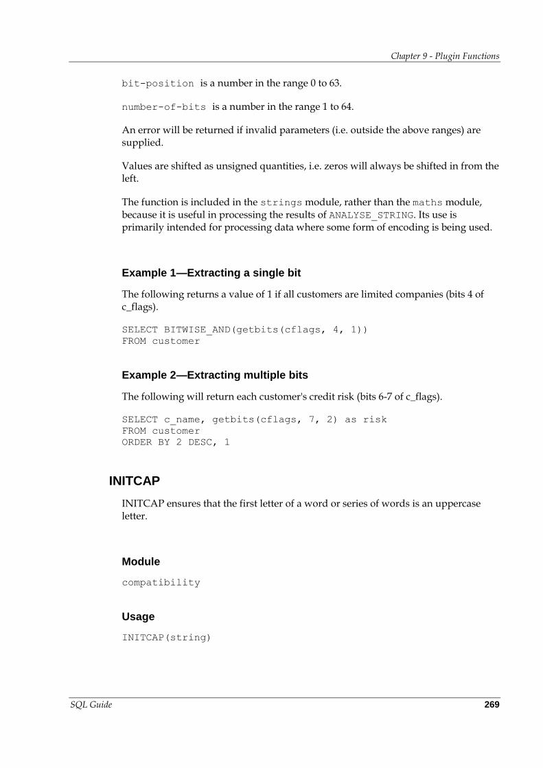
Chapter 9 - Plugin Functions
SQL Guide 269
bit-position is a number in the range 0 to 63.
number-of-bits is a number in the range 1 to 64.
An error will be returned if invalid parameters (i.e. outside the above ranges) are supplied.
Values are shifted as unsigned quantities, i.e. zeros will always be shifted in from the left.
The function is included in the strings module, rather than the maths module, because it is useful in processing the results of ANALYSE_STRING. Its use is primarily intended for processing data where some form of encoding is being used.
Example 1—Extracting a single bit
The following returns a value of 1 if all customers are limited companies (bits 4 of c_flags).
SELECT BITWISE_AND(getbits(cflags, 4, 1))
FROM customer
Example 2—Extracting multiple bits
The following will return each customer's credit risk (bits 6-7 of c_flags).
SELECT c_name, getbits(cflags, 7, 2) as risk
FROM customer
ORDER BY 2 DESC, 1
INITCAP
INITCAP ensures that the first letter of a word or series of words is an uppercase letter.
Module
compatibility
Usage
INITCAP(string)
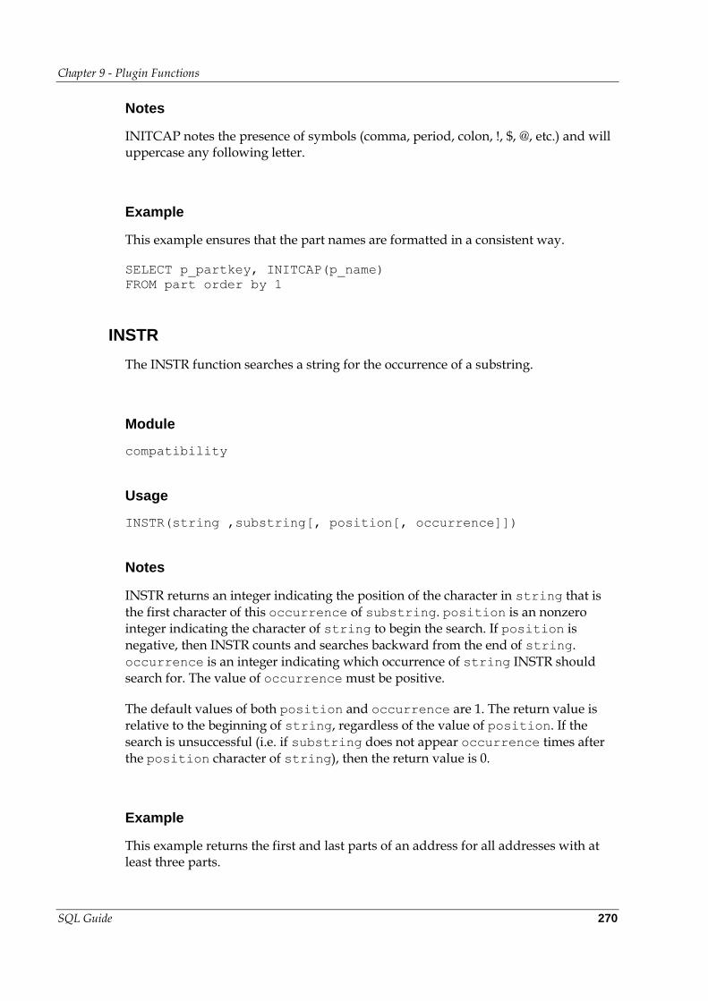
Chapter 9 - Plugin Functions
SQL Guide 270
Notes
INITCAP notes the presence of symbols (comma, period, colon, !, $, @, etc.) and will uppercase any following letter.
Example
This example ensures that the part names are formatted in a consistent way.
SELECT p_partkey, INITCAP(p_name)
FROM part order by 1
INSTR
The INSTR function searches a string for the occurrence of a substring.
Module
compatibility
Usage
INSTR(string ,substring[, position[, occurrence]])
Notes
INSTR returns an integer indicating the position of the character in string that is the first character of this occurrence of substring. position is an nonzero integer indicating the character of string to begin the search. If position is negative, then INSTR counts and searches backward from the end of string. occurrence is an integer indicating which occurrence of string INSTR should search for. The value of occurrence must be positive.
The default values of both position and occurrence are 1. The return value is relative to the beginning of string, regardless of the value of position. If the search is unsuccessful (i.e. if substring does not appear occurrence times after the position character of string), then the return value is 0.
Example
This example returns the first and last parts of an address for all addresses with at least three parts.
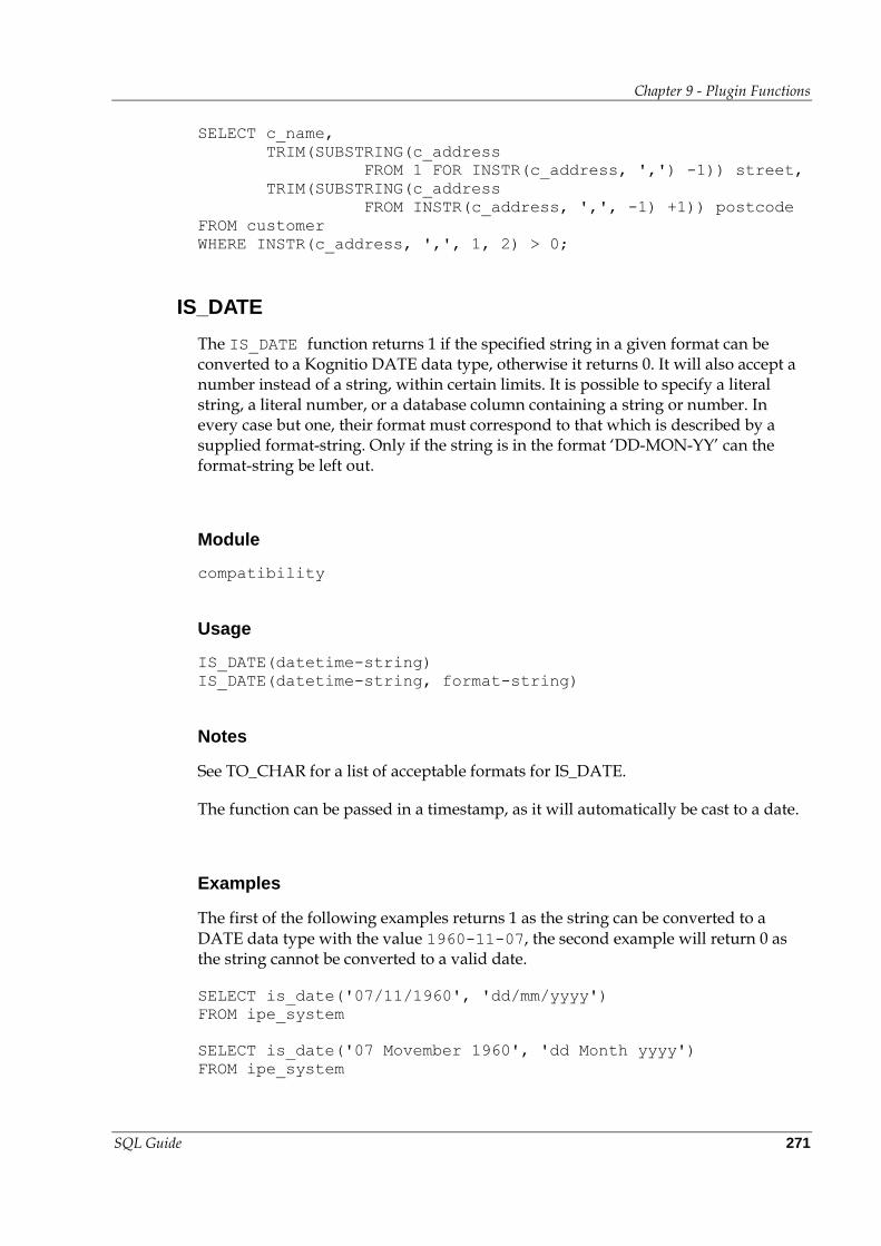
Chapter 9 - Plugin Functions
SQL Guide 271
SELECT c_name,
TRIM(SUBSTRING(c_address
FROM 1 FOR INSTR(c_address, ',') -1)) street,
TRIM(SUBSTRING(c_address
FROM INSTR(c_address, ',', -1) +1)) postcode
FROM customer
WHERE INSTR(c_address, ',', 1, 2) > 0;
IS_DATE
The IS_DATE function returns 1 if the specified string in a given format can be converted to a Kognitio DATE data type, otherwise it returns 0. It will also accept a number instead of a string, within certain limits. It is possible to specify a literal string, a literal number, or a database column containing a string or number. In every case but one, their format must correspond to that which is described by a supplied format-string. Only if the string is in the format ‘DD-MON-YY’ can the format-string be left out.
Module
compatibility
Usage
IS_DATE(datetime-string)
IS_DATE(datetime-string, format-string)
Notes
See TO_CHAR for a list of acceptable formats for IS_DATE.
The function can be passed in a timestamp, as it will automatically be cast to a date.
Examples
The first of the following examples returns 1 as the string can be converted to a DATE data type with the value 1960-11-07, the second example will return 0 as the string cannot be converted to a valid date.
SELECT is_date('07/11/1960', 'dd/mm/yyyy')
FROM ipe_system
SELECT is_date('07 Movember 1960', 'dd Month yyyy')
FROM ipe_system
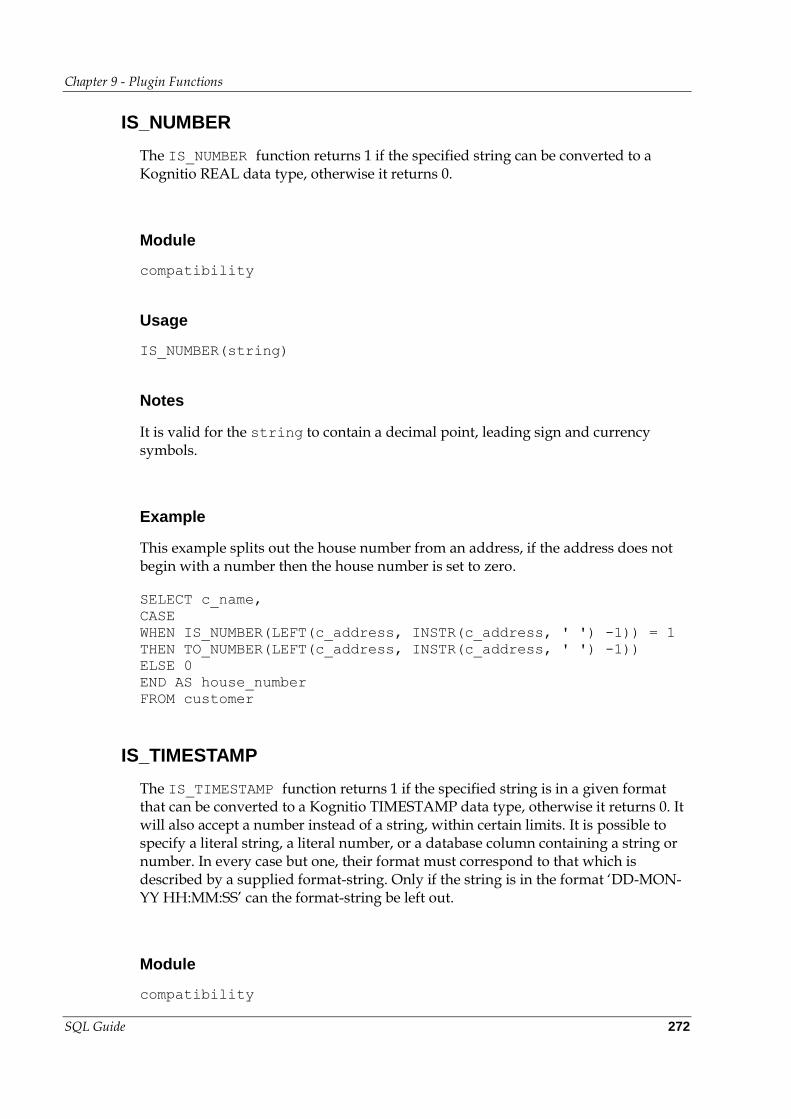
Chapter 9 - Plugin Functions
SQL Guide 272
IS_NUMBER
The IS_NUMBER function returns 1 if the specified string can be converted to a Kognitio REAL data type, otherwise it returns 0.
Module
compatibility
Usage
IS_NUMBER(string)
Notes
It is valid for the string to contain a decimal point, leading sign and currency symbols.
Example
This example splits out the house number from an address, if the address does not begin with a number then the house number is set to zero.
SELECT c_name,
CASE
WHEN IS_NUMBER(LEFT(c_address, INSTR(c_address, ' ') -1)) = 1
THEN TO_NUMBER(LEFT(c_address, INSTR(c_address, ' ') -1))
ELSE 0
END AS house_number
FROM customer
IS_TIMESTAMP
The IS_TIMESTAMP function returns 1 if the specified string is in a given format that can be converted to a Kognitio TIMESTAMP data type, otherwise it returns 0. It will also accept a number instead of a string, within certain limits. It is possible to specify a literal string, a literal number, or a database column containing a string or number. In every case but one, their format must correspond to that which is described by a supplied format-string. Only if the string is in the format ‘DD-MON-YY HH:MM:SS’ can the format-string be left out.
Module
compatibility
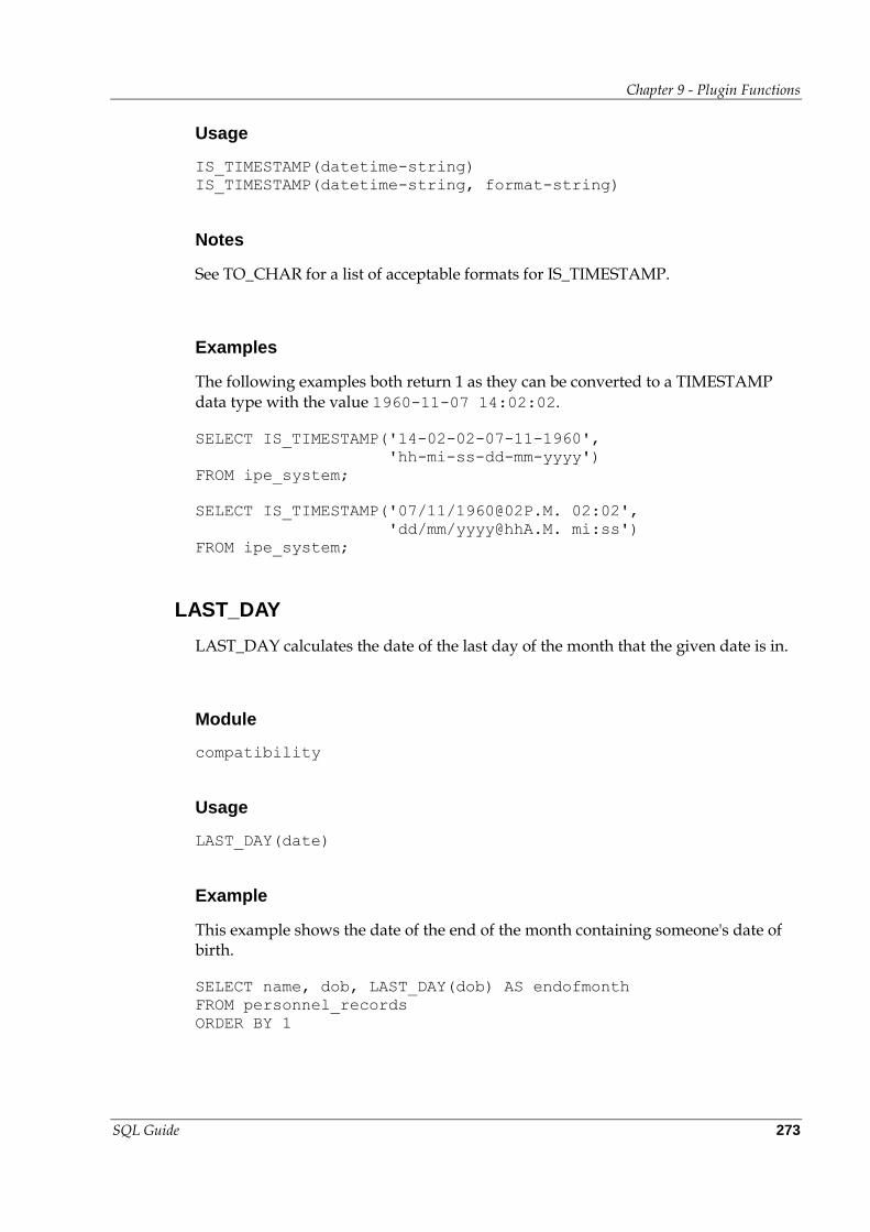
Chapter 9 - Plugin Functions
SQL Guide 273
Usage
IS_TIMESTAMP(datetime-string)
IS_TIMESTAMP(datetime-string, format-string)
Notes
See TO_CHAR for a list of acceptable formats for IS_TIMESTAMP.
Examples
The following examples both return 1 as they can be converted to a TIMESTAMP data type with the value 1960-11-07 14:02:02.
SELECT IS_TIMESTAMP('14-02-02-07-11-1960',
'hh-mi-ss-dd-mm-yyyy')
FROM ipe_system;
SELECT IS_TIMESTAMP('07/11/[email protected]. 02:02',
'dd/mm/[email protected]. mi:ss')
FROM ipe_system;
LAST_DAY
LAST_DAY calculates the date of the last day of the month that the given date is in.
Module
compatibility
Usage
LAST_DAY(date)
Example
This example shows the date of the end of the month containing someone's date of birth.
SELECT name, dob, LAST_DAY(dob) AS endofmonth
FROM personnel_records
ORDER BY 1
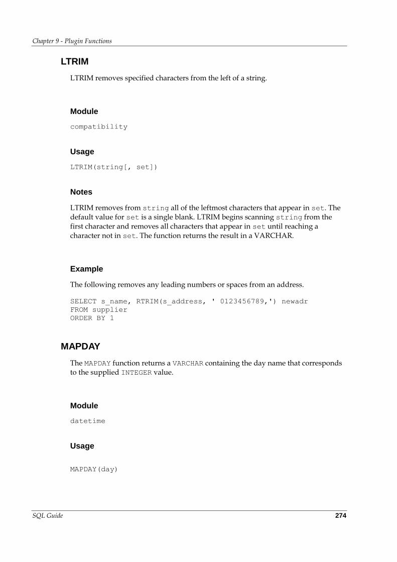
Chapter 9 - Plugin Functions
SQL Guide 274
LTRIM
LTRIM removes specified characters from the left of a string.
Module
compatibility
Usage
LTRIM(string[, set])
Notes
LTRIM removes from string all of the leftmost characters that appear in set. The default value for set is a single blank. LTRIM begins scanning string from the first character and removes all characters that appear in set until reaching a character not in set. The function returns the result in a VARCHAR.
Example
The following removes any leading numbers or spaces from an address.
SELECT s_name, RTRIM(s_address, ' 0123456789,') newadr
FROM supplier
ORDER BY 1
MAPDAY
The MAPDAY function returns a VARCHAR containing the day name that corresponds to the supplied INTEGER value.
Module
datetime
Usage
MAPDAY(day)
Chapter 9 - Plugin Functions
SQL Guide 275
Notes
An error will be returned if day is not in the range 0–6 (Sunday–Saturday).
Example
This example shows the day on which someone was born.
SELECT name, dob, MAPDAY(DAYOFWEEK(dob)) as dow
FROM personnel_records
ORDER BY 3, 2, 1
MAPMONTH
The MAPMONTH function returns a VARCHAR containing the month name that corresponds to the supplied INTEGER value.
Module
datetime
Usage
MAPMONTH(month)
Notes
An error will be returned if month is not in the range 1–12 (January–December).
Example
This example shows the month in which someone was born.
SELECT name, dob,
MAPMONTH(DT_INFO(dob, 'monthofyear')) as moy
FROM personnel_records
ORDER BY 3, 2, 1
MONTHS_BETWEEN
MONTHS_BETWEEN calculates the difference between two dates in months.
Chapter 9 - Plugin Functions
SQL Guide 276
Module
Compatibility
Usage
MONTHS_BETWEEN(date1, date2)
Notes
The function calculates date1 - date2. The result is normally not an integer.
Example
This example sums orders received from individual customers during the last month.
SELECT o_custkey, SUM(o_totalprice)
FROM ordertab
WHERE MONTHS_BETWEEN(SYSDATE, o_orderdate) BETWEEN 0 AND 1
GROUP BY 1
ORDER BY 2 DESC, 1
NEXT_DAY
NEXT_DAY calculates the date of the next named day of the week (that is, Sunday, Monday, Tuesday, Wednesday, Thursday, Friday and Saturday), after the given date.
Module
compatibility
Usage
NEXT_DAY(date, day-string)
Notes
NEXT_DAY is a “greater than” function, asking for the next date greater than the given date that falls on a particular day. This means that if the given date occurs on the specified day, the function will return the date of the next specified day. To make NEXT_DAY a “greater than or equal” function, subtract 1 from the date.
Chapter 9 - Plugin Functions
SQL Guide 277
Example
This example generates the date of the next payday, which is always the last Friday of the month.
SELECT
NEXT_DAY(LAST_DAY(SYSDATE) - INTERVAL '7' DAY, 'friday')
FROM ipe_system;
PROFILE
The PROFILE function allows character strings to be profiled. It is typically used in data auditing to look for repeated format patterns in string data.
Module
strings
Usage
PROFILE(mode, string)
Notes
The function uses the following characters to profile character data:
A Upper case alpha (A-Z)
a Lower case alpha (a-z)
N Numeric (0-9)
P Punctuation (.,;'@$ etc.)
S space (space or tab)
X non-printable
The function has three modes:
1. Perform a one-to-one mapping between string data and profiling characters
2. Collapse and count repeated character profiles (aaa := 3a)
3. Collapse repeated character profiles (aaa := a)
Notes: Use SUBSTRING to limit the profiling to a specific area of a character string.
Use TRIM to remove trailing spaces prior to profiling if the spaces are not significant.
Chapter 9 - Plugin Functions
SQL Guide 278
Example—Profile a simple string
This example shows the output of PROFILE for a simple string using each of the modes.
SELECT p_name,
PROFILE(1, p_name) AS m1,
PROFILE(2, p_name) AS m2,
PROFILE(3, p_name) as m3
FROM part
WHERE p_name = 'Pump:3 Speed'
ORDER BY 1
p_name m1 m2 m3
Pump:3 Speed AaaaPNSAaaaa A3aPNSA4a AaPNSAa
REPLACE
The REPLACE function replaces one or more characters in a string with 0 or more characters.
Module
compatibility
Usage
REPLACE(string, search-string, replace-string)
Notes
Every occurrence of search-string is replaced by replace-string.
Example—Replace mistyped words
This example corrects some comments that were entered with incorrect dates.
SELECT p_name,
REPLACE(p_comment, '2003', '2004') corrected_year
FROM part
ORDER BY 1
REVERSE
The REVERSE function takes a string and reverses the characters within it. The result is returned in a VARCHAR.
Chapter 9 - Plugin Functions
SQL Guide 279
Module
strings
Usage
REVERSE(source-string)
Notes
source-string is the string to process.
Example 1—Find possible palindromes
SELECT *
FROM possible_palindromes
WHERE TRIM(LOWER(wrd)) = TRIM(LOWER(REVERSE(wrd)))
Note The TRIM and LOWER functions ensure we ignore any leading/trailing spaces and case differences.
Example 2—Extract a trailing initial
This example extracts the initial from a list of names that are stored in the form “Surname Initial”.
SELECT SUBSTRING(REVERSE(name) FROM 1 FOR 1) AS initial
FROM names
Note This method avoids the need to use the CHAR_LENGTH or POSITION functions to find the position of the last character.
ROUND
The ROUND function returns the supplied argument rounded to the nearest whole value.
Module
compatibility
Usage
ROUND(number[, m])
ROUND(timestamp[, fmt])
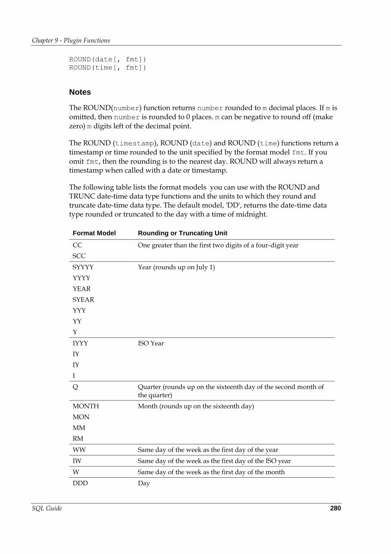
Chapter 9 - Plugin Functions
SQL Guide 280
ROUND(date[, fmt])
ROUND(time[, fmt])
Notes
The ROUND(number) function returns number rounded to m decimal places. If m is omitted, then number is rounded to 0 places. m can be negative to round off (make zero) m digits left of the decimal point.
The ROUND (timestamp), ROUND (date) and ROUND (time) functions return a timestamp or time rounded to the unit specified by the format model fmt. If you
omit fmt, then the rounding is to the nearest day. ROUND will always return a timestamp when called with a date or timestamp.
The following table lists the format models you can use with the ROUND and TRUNC date-time data type functions and the units to which they round and truncate date-time data type. The default model, 'DD', returns the date-time data type rounded or truncated to the day with a time of midnight.
Format Model Rounding or Truncating Unit
CC One greater than the first two digits of a four-digit year
SCC
SYYYY Year (rounds up on July 1)
YYYY
YEAR
SYEAR
YYY
YY
Y
IYYY ISO Year
IY
IY
I
Q Quarter (rounds up on the sixteenth day of the second month of the quarter)
MONTH Month (rounds up on the sixteenth day)
MON
MM
RM
WW Same day of the week as the first day of the year
IW Same day of the week as the first day of the ISO year
W Same day of the week as the first day of the month
DDD Day
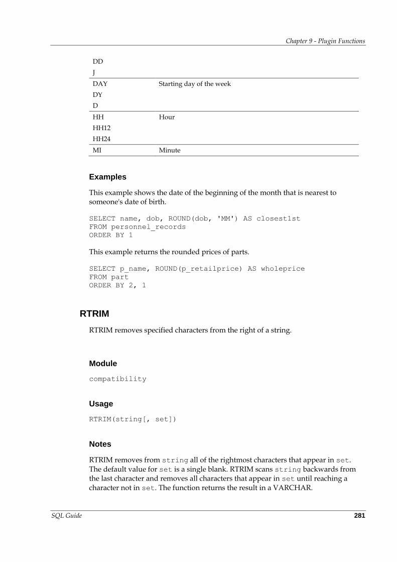
Chapter 9 - Plugin Functions
SQL Guide 281
DD
J
DAY Starting day of the week
DY
D
HH Hour
HH12
HH24
MI Minute
Examples
This example shows the date of the beginning of the month that is nearest to someone's date of birth.
SELECT name, dob, ROUND(dob, 'MM') AS closest1st
FROM personnel_records
ORDER BY 1
This example returns the rounded prices of parts.
SELECT p_name, ROUND(p_retailprice) AS wholeprice
FROM part
ORDER BY 2, 1
RTRIM
RTRIM removes specified characters from the right of a string.
Module
compatibility
Usage
RTRIM(string[, set])
Notes
RTRIM removes from string all of the rightmost characters that appear in set. The default value for set is a single blank. RTRIM scans string backwards from the last character and removes all characters that appear in set until reaching a
character not in set. The function returns the result in a VARCHAR.
Chapter 9 - Plugin Functions
SQL Guide 282
Example
The following removes any trailing punctation or spaces from an address.
SELECT s_name, RTRIM(s_address, ' .,') newadr
FROM supplier
ORDER BY 1
SINKCHARS
The SINKCHARS function takes a string and removes (sinks) a series of characters
from it. The result is returned as a VARCHAR.
Module
strings
Usage
SINKCHARS(source-string, char-string)
SINKCHARS(source-string)
Notes
source-string is the string to process.
char-string is a list of characters to remove.
The default char-string is all non-printable characters.
All occurrences of the characters in char-string will be removed from source-string.
The order the character appear in char-string is unimportant.
Example 1—Remove any non-printable characters from an address
This example removes any non-printable characters from a supplier's address.
SELECT s_name,
SINKCHARS(s_address) newadr
FROM supplier
ORDER BY 1
Chapter 9 - Plugin Functions
SQL Guide 283
Example 2—Remove punctation from an address
This example removes any parentheses and spaces from a supplier's phone number.
SELECT s_name,
SINKCHARS(s_phone, ' ()') newphone
FROM supplier
ORDER BY 1
SNIPCHARS
The SNIPCHARS function takes a string and removes a series of characters from the beginning and/or end of it. The result is returned as a VARCHAR.
Module
strings
Usage
SNIPCHARS(source-string, char-string, control-string)
SNIPCHARS(source-string, char-string)
SNIPCHARS(source-string)
Notes
source-string is the string to process.
char-string is a list of characters to trim.
control-string is one of BOTH, LEADING or TRAILING.
control-string is not case sensitive and can contain trailing spaces.
control-string has to be enclosed in single quotes.
The default char-string is white space (space & tab).
The default control-string is BOTH.
The order the character appear in char-string is unimportant.
Using SNIPCHARS to remove a single character is equivalent to the standard TRIM function.
Chapter 9 - Plugin Functions
SQL Guide 284
Example 1—Remove any trailing punctuation from an address
This example removes any spaces, full stops or commas from the end of a supplier's address.
SELECT s_name,
SNIPCHARS(s_address, ' .,', 'trailing') newadr
FROM supplier
ORDER BY 1
Example 2—Remove any leading digits from an address
This example removes any leading digits and spaces from the beginning of a supplier's address.
SELECT s_name,
SNIPCHARS(s_address, ' 0123456789', 'leading') newadr
FROM supplier
ORDER BY 1
SUBSTR
The SUBSTR function returns a substring of a string.
Module
compatibility
Usage
SUBSTR(string, pos[ , len])
Notes
SUBSTR can only be used with character strings.
Using the built-in Kognitio function SUBSTRING which has exactly the same parameters will eliminate the overhead associated with using plugin functions.
Chapter 9 - Plugin Functions
SQL Guide 285
Example – Outgoing Postcode
You can select the last three characters of a UK postcode, which form the “outgoing” part. These are useful for surveys based on a single postal district. As the length of incoming postcodes vary from three to four characters (for example, ST1, ST13) followed by a space, the outgoing codes start either at position 5 or position 6. This means that the new postcode column has a space before the code, where the incoming postcode has only three characters. You can remove the unwanted spaces using TRIM.
CREATE VIEW outward_postcode(name, address, postcode) AS
SELECT c_name, c_address,
TRIM(SUBSTR(c_postcode, 5, 4))
FROM customer
SUCKCHARS
The SUCKCHARS function takes a string and extracts (sucks) from it the string contained within it that is bounded by two other strings. The result is returned as a VARCHAR.
Module
strings
Usage
SUCKCHARS(source-string, start-string, end-string)
Notes
source-string is the string to process.
start-string is the string that indicates the leading boundary of the string to extract.
end-string is the string that indicates the trailing boundary of the string to extract.
If start-string doesn't exist we return data from the first position of source-string.
If end-string doesn't exist we keep going to the end of source-string.
end-string has to appear after start-string.
Either or both of start-string and end-string can be zero length, in which case they are ignored.
Chapter 9 - Plugin Functions
SQL Guide 286
start-string is looked for from the left, end-string from the right.
There is currently no way to say you want to find the nth occurrence of either start-string or end-string.
Example—Splitting up telephone numbers
This example returns a telephone number as a separate area code and number. The numbers are specified in one of two ways, depending on whether it was supplied with a county code prefix, e.g. (01344)300770 or +44(0)1344 300770.
SELECT SUCKCHARS(s_phone, '(', ')') code,
SUCKCHARS(s_phone, ')', '') no
FROM supplier
WHERE s_phone LIKE('(%')
UNION
SELECT '0' ||
SUCKCHARS(TRIM(s_phone), '(0)', ' ') code,
SUCKCHARS(s_phone, ' ', '') no
FROM supplier
WHERE s_phone LIKE('+%')
ORDER BY 1
Note: We require a TRIM (or a CAST to a VARCHAR), in the second UNION—Otherwise we will use any trailing spaces in the CHAR column as our end-string and hence return the entire number as the code.
SWAPCHARS
The SWAPCHARS function takes a string and swaps characters according to the form in which it is called. The result is returned in a VARCHAR.
Module
strings
Usage
SWAPCHARS(source-string)
SWAPCHARS(source-string, replacement-character)
SWAPCHARS(source-string, from-string, to-string)
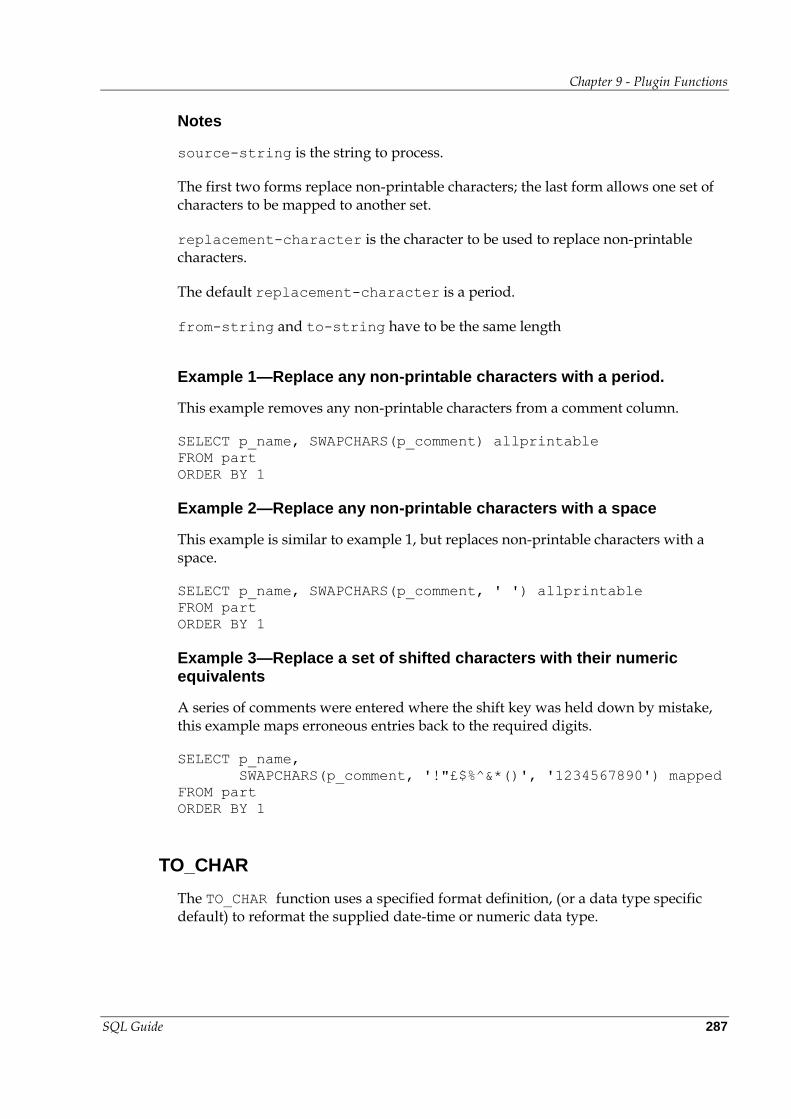
Chapter 9 - Plugin Functions
SQL Guide 287
Notes
source-string is the string to process.
The first two forms replace non-printable characters; the last form allows one set of characters to be mapped to another set.
replacement-character is the character to be used to replace non-printable characters.
The default replacement-character is a period.
from-string and to-string have to be the same length
Example 1—Replace any non-printable characters with a period.
This example removes any non-printable characters from a comment column.
SELECT p_name, SWAPCHARS(p_comment) allprintable
FROM part
ORDER BY 1
Example 2—Replace any non-printable characters with a space
This example is similar to example 1, but replaces non-printable characters with a space.
SELECT p_name, SWAPCHARS(p_comment, ' ') allprintable
FROM part
ORDER BY 1
Example 3—Replace a set of shifted characters with their numeric equivalents
A series of comments were entered where the shift key was held down by mistake, this example maps erroneous entries back to the required digits.
SELECT p_name,
SWAPCHARS(p_comment, '!"£$%^&*()', '1234567890') mapped
FROM part
ORDER BY 1
TO_CHAR
The TO_CHAR function uses a specified format definition, (or a data type specific default) to reformat the supplied date-time or numeric data type.
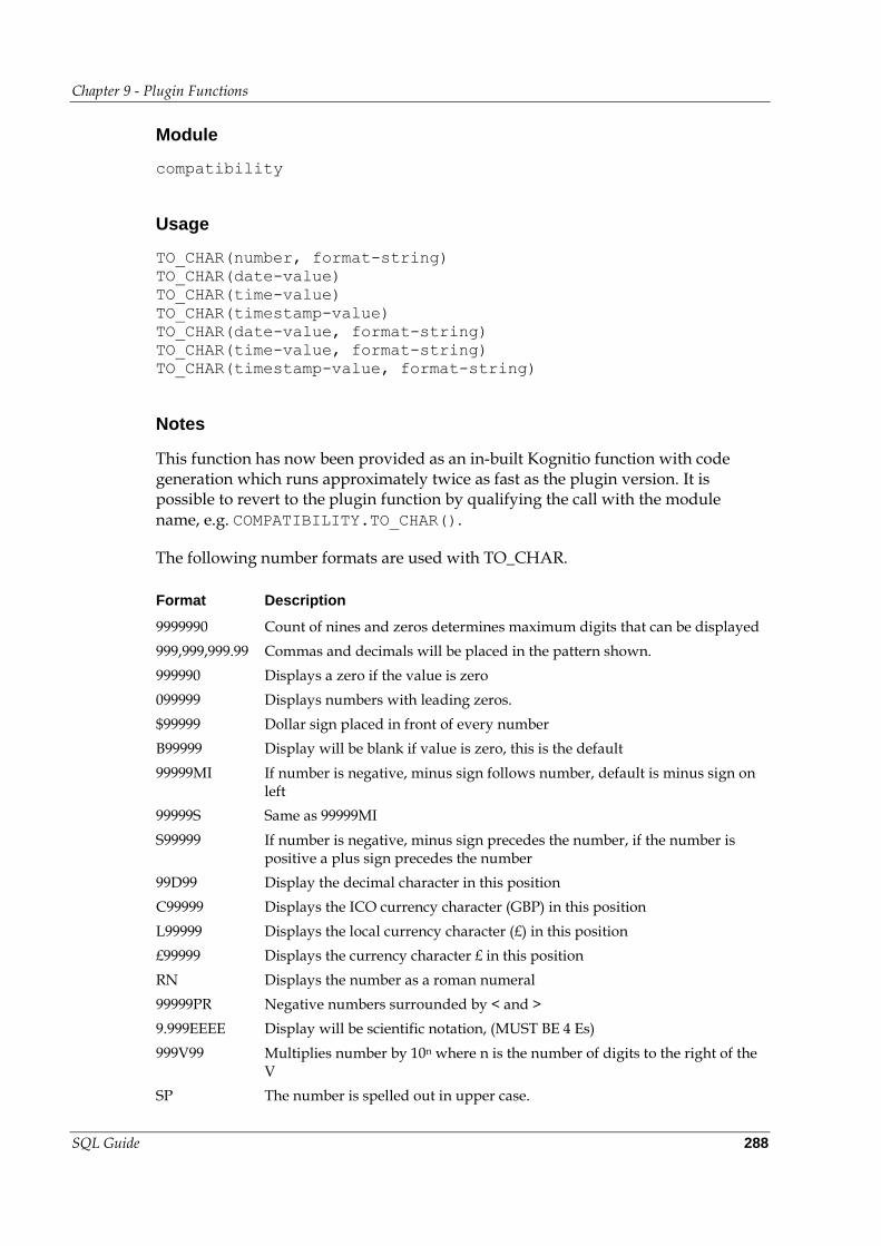
Chapter 9 - Plugin Functions
SQL Guide 288
Module
compatibility
Usage
TO_CHAR(number, format-string)
TO_CHAR(date-value)
TO_CHAR(time-value)
TO_CHAR(timestamp-value)
TO_CHAR(date-value, format-string)
TO_CHAR(time-value, format-string)
TO_CHAR(timestamp-value, format-string)
Notes
This function has now been provided as an in-built Kognitio function with code generation which runs approximately twice as fast as the plugin version. It is possible to revert to the plugin function by qualifying the call with the module name, e.g. COMPATIBILITY.TO_CHAR().
The following number formats are used with TO_CHAR.
Format Description
9999990 Count of nines and zeros determines maximum digits that can be displayed
999,999,999.99 Commas and decimals will be placed in the pattern shown.
999990 Displays a zero if the value is zero
099999 Displays numbers with leading zeros.
$99999 Dollar sign placed in front of every number
B99999 Display will be blank if value is zero, this is the default
99999MI If number is negative, minus sign follows number, default is minus sign on left
99999S Same as 99999MI
S99999 If number is negative, minus sign precedes the number, if the number is positive a plus sign precedes the number
99D99 Display the decimal character in this position
C99999 Displays the ICO currency character (GBP) in this position
L99999 Displays the local currency character (£) in this position
£99999 Displays the currency character £ in this position
RN Displays the number as a roman numeral
99999PR Negative numbers surrounded by < and >
9.999EEEE Display will be scientific notation, (MUST BE 4 Es)
999V99 Multiplies number by 10n where n is the number of digits to the right of the V
SP The number is spelled out in upper case.
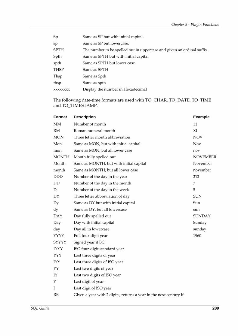
Chapter 9 - Plugin Functions
SQL Guide 289
Sp Same as SP but with initial capital.
sp Same as SP but lowercase.
SPTH The number to be spelled out in uppercase and given an ordinal suffix.
Spth Same as SPTH but with initial capital.
spth Same as SPTH but lower case.
THSP Same as SPTH
Thsp Same as Spth
thsp Same as spth
xxxxxxxx Display the number in Hexadecimal
The following date-time formats are used with TO_CHAR, TO_DATE, TO_TIME and TO_TIMESTAMP.
Format Description Example
MM Number of month 11
RM Roman numeral month XI
MON Three letter month abbreviation NOV
Mon Same as MON, but with initial capital Nov
mon Same as MON, but all lower case nov
MONTH Month fully spelled out NOVEMBER
Month Same as MONTH, but with initial capital November
month Same as MONTH, but all lower case november
DDD Number of the day in the year 312
DD Number of the day in the month 7
D Number of the day in the week 5
DY Three letter abbreviation of day SUN
Dy Same as DY but with initial capital Sun
dy Same as DY, but all lowercase sun
DAY Day fully spelled out SUNDAY
Day Day with initial capital Sunday
day Day all in lowercase sunday
YYYY Full four-digit year 1960
SYYYY Signed year if BC
IYYY ISO four-digit standard year
YYY Last three digits of year
IYY Last three digits of ISO year
YY Last two digits of year
IY Last two digits of ISO year
Y Last digit of year
I Last digit of ISO year
RR Given a year with 2 digits, returns a year in the next century if
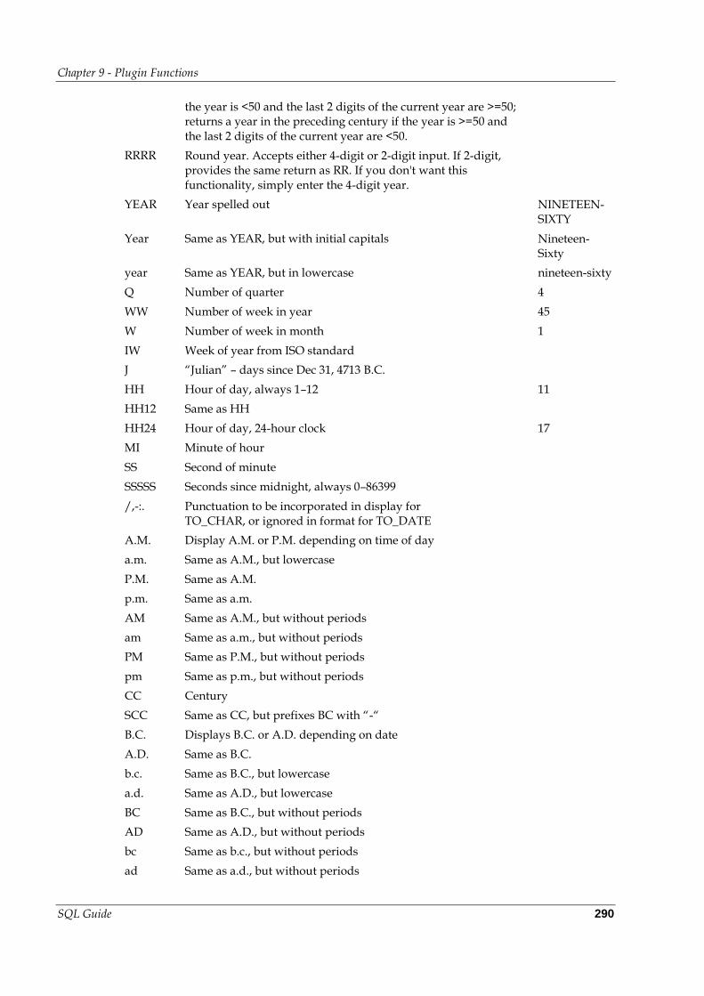
Chapter 9 - Plugin Functions
SQL Guide 290
the year is <50 and the last 2 digits of the current year are >=50; returns a year in the preceding century if the year is >=50 and the last 2 digits of the current year are <50.
RRRR Round year. Accepts either 4-digit or 2-digit input. If 2-digit, provides the same return as RR. If you don't want this functionality, simply enter the 4-digit year.
YEAR Year spelled out NINETEEN-SIXTY
Year Same as YEAR, but with initial capitals Nineteen-Sixty
year Same as YEAR, but in lowercase nineteen-sixty
Q Number of quarter 4
WW Number of week in year 45
W Number of week in month 1
IW Week of year from ISO standard
J “Julian” – days since Dec 31, 4713 B.C.
HH Hour of day, always 1–12 11
HH12 Same as HH
HH24 Hour of day, 24-hour clock 17
MI Minute of hour
SS Second of minute
SSSSS Seconds since midnight, always 0–86399
/,-:. Punctuation to be incorporated in display for TO_CHAR, or ignored in format for TO_DATE
A.M. Display A.M. or P.M. depending on time of day
a.m. Same as A.M., but lowercase
P.M. Same as A.M.
p.m. Same as a.m.
AM Same as A.M., but without periods
am Same as a.m., but without periods
PM Same as P.M., but without periods
pm Same as p.m., but without periods
CC Century
SCC Same as CC, but prefixes BC with “-“
B.C. Displays B.C. or A.D. depending on date
A.D. Same as B.C.
b.c. Same as B.C., but lowercase
a.d. Same as A.D., but lowercase
BC Same as B.C., but without periods
AD Same as A.D., but without periods
bc Same as b.c., but without periods
ad Same as a.d., but without periods
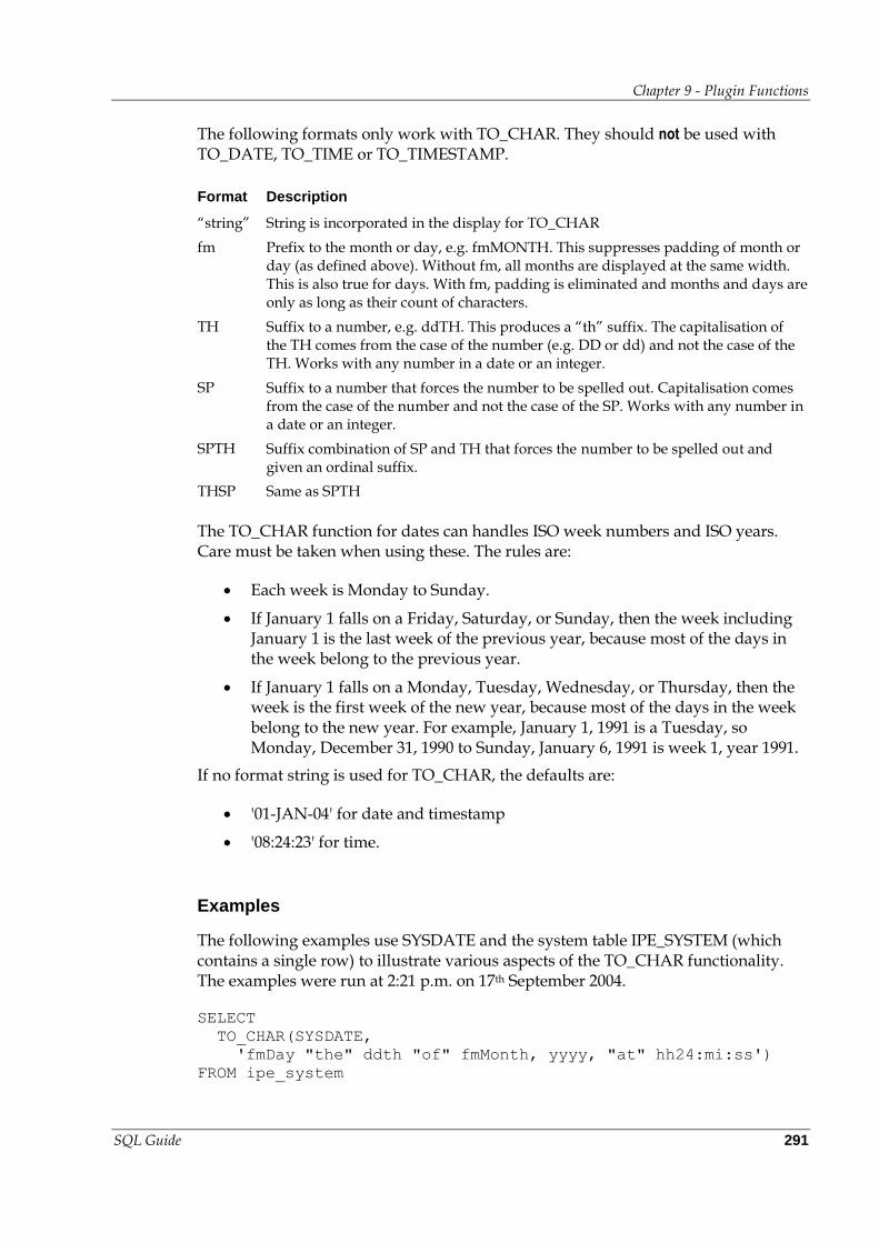
Chapter 9 - Plugin Functions
SQL Guide 291
The following formats only work with TO_CHAR. They should not be used with TO_DATE, TO_TIME or TO_TIMESTAMP.
Format Description
“string” String is incorporated in the display for TO_CHAR
fm Prefix to the month or day, e.g. fmMONTH. This suppresses padding of month or day (as defined above). Without fm, all months are displayed at the same width. This is also true for days. With fm, padding is eliminated and months and days are only as long as their count of characters.
TH Suffix to a number, e.g. ddTH. This produces a “th” suffix. The capitalisation of the TH comes from the case of the number (e.g. DD or dd) and not the case of the TH. Works with any number in a date or an integer.
SP Suffix to a number that forces the number to be spelled out. Capitalisation comes from the case of the number and not the case of the SP. Works with any number in a date or an integer.
SPTH Suffix combination of SP and TH that forces the number to be spelled out and given an ordinal suffix.
THSP Same as SPTH
The TO_CHAR function for dates can handles ISO week numbers and ISO years. Care must be taken when using these. The rules are:
Each week is Monday to Sunday.
If January 1 falls on a Friday, Saturday, or Sunday, then the week including January 1 is the last week of the previous year, because most of the days in the week belong to the previous year.
If January 1 falls on a Monday, Tuesday, Wednesday, or Thursday, then the week is the first week of the new year, because most of the days in the week belong to the new year. For example, January 1, 1991 is a Tuesday, so Monday, December 31, 1990 to Sunday, January 6, 1991 is week 1, year 1991.
If no format string is used for TO_CHAR, the defaults are:
'01-JAN-04' for date and timestamp
'08:24:23' for time.
Examples
The following examples use SYSDATE and the system table IPE_SYSTEM (which contains a single row) to illustrate various aspects of the TO_CHAR functionality. The examples were run at 2:21 p.m. on 17th September 2004.
SELECT
TO_CHAR(SYSDATE,
'fmDay "the" ddth "of" fmMonth, yyyy, "at" hh24:mi:ss')
FROM ipe_system
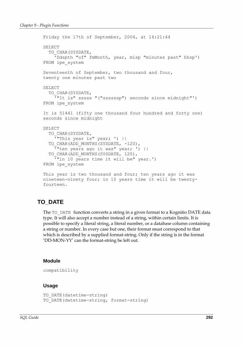
Chapter 9 - Plugin Functions
SQL Guide 292
Friday the 17th of September, 2004, at 14:21:44
SELECT
TO_CHAR(SYSDATE,
'Ddspth "of" fmMonth, year, misp "minutes past" hhsp')
FROM ipe_system
Seventeenth of September, two thousand and four,
twenty one minutes past two
SELECT
TO_CHAR(SYSDATE,
'"It is" sssss "("ssssssp") seconds since midnight"')
FROM ipe_system
It is 51441 (fifty one thousand four hundred and forty one)
seconds since midnight
SELECT
TO_CHAR(SYSDATE,
'"This year is" year; ') ||
TO_CHAR(ADD_MONTHS(SYSDATE, -120),
'"ten years ago it was" year; ') ||
TO_CHAR(ADD_MONTHS(SYSDATE, 120),
'"in 10 years time it will be" year.')
FROM ipe_system
This year is two thousand and four; ten years ago it was
nineteen-ninety four; in 10 years time it will be twenty-
fourteen.
TO_DATE
The TO_DATE function converts a string in a given format to a Kognitio DATE data type. It will also accept a number instead of a string, within certain limits. It is possible to specify a literal string, a literal number, or a database column containing a string or number. In every case but one, their format must correspond to that which is described by a supplied format-string. Only if the string is in the format ‘DD-MON-YY’ can the format-string be left out.
Module
compatibility
Usage
TO_DATE(datetime-string)
TO_DATE(datetime-string, format-string)
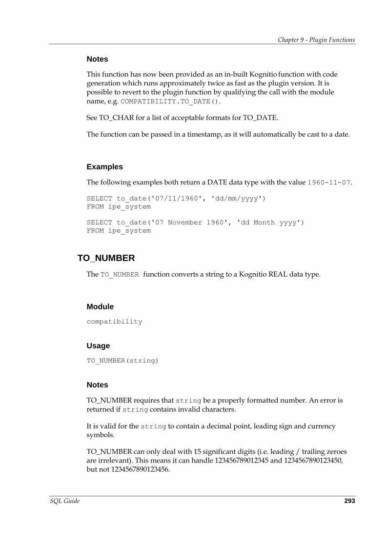
Chapter 9 - Plugin Functions
SQL Guide 293
Notes
This function has now been provided as an in-built Kognitio function with code generation which runs approximately twice as fast as the plugin version. It is possible to revert to the plugin function by qualifying the call with the module name, e.g. COMPATIBILITY.TO_DATE().
See TO_CHAR for a list of acceptable formats for TO_DATE.
The function can be passed in a timestamp, as it will automatically be cast to a date.
Examples
The following examples both return a DATE data type with the value 1960-11-07.
SELECT to_date('07/11/1960', 'dd/mm/yyyy')
FROM ipe_system
SELECT to_date('07 November 1960', 'dd Month yyyy')
FROM ipe_system
TO_NUMBER
The TO_NUMBER function converts a string to a Kognitio REAL data type.
Module
compatibility
Usage
TO_NUMBER(string)
Notes
TO_NUMBER requires that string be a properly formatted number. An error is returned if string contains invalid characters.
It is valid for the string to contain a decimal point, leading sign and currency symbols.
TO_NUMBER can only deal with 15 significant digits (i.e. leading / trailing zeroes are irrelevant). This means it can handle 123456789012345 and 1234567890123450, but not 1234567890123456.
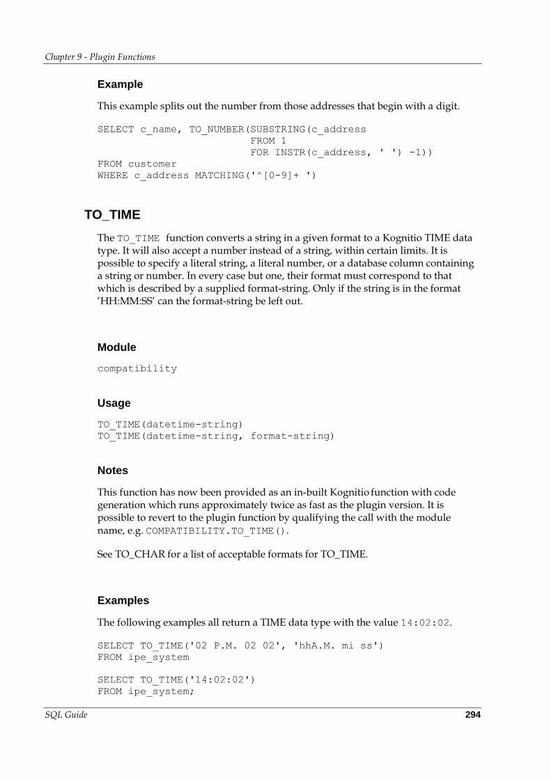
Chapter 9 - Plugin Functions
SQL Guide 294
Example
This example splits out the number from those addresses that begin with a digit.
SELECT c_name, TO_NUMBER(SUBSTRING(c_address
FROM 1
FOR INSTR(c_address, ' ') -1))
FROM customer
WHERE c_address MATCHING('^[0-9]+ ')
TO_TIME
The TO_TIME function converts a string in a given format to a Kognitio TIME data type. It will also accept a number instead of a string, within certain limits. It is possible to specify a literal string, a literal number, or a database column containing a string or number. In every case but one, their format must correspond to that which is described by a supplied format-string. Only if the string is in the format ‘HH:MM:SS’ can the format-string be left out.
Module
compatibility
Usage
TO_TIME(datetime-string)
TO_TIME(datetime-string, format-string)
Notes
This function has now been provided as an in-built Kognitio function with code generation which runs approximately twice as fast as the plugin version. It is possible to revert to the plugin function by qualifying the call with the module name, e.g. COMPATIBILITY.TO_TIME().
See TO_CHAR for a list of acceptable formats for TO_TIME.
Examples
The following examples all return a TIME data type with the value 14:02:02.
SELECT TO_TIME('02 P.M. 02 02', 'hhA.M. mi ss')
FROM ipe_system
SELECT TO_TIME('14:02:02')
FROM ipe_system;
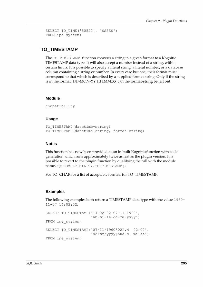
Chapter 9 - Plugin Functions
SQL Guide 295
SELECT TO_TIME('50522', 'SSSSS')
FROM ipe_system;
TO_TIMESTAMP
The TO_TIMESTAMP function converts a string in a given format to a Kognitio TIMESTAMP data type. It will also accept a number instead of a string, within certain limits. It is possible to specify a literal string, a literal number, or a database column containing a string or number. In every case but one, their format must correspond to that which is described by a supplied format-string. Only if the string is in the format ‘DD-MON-YY HH:MM:SS’ can the format-string be left out.
Module
compatibility
Usage
TO_TIMESTAMP(datetime-string)
TO_TIMESTAMP(datetime-string, format-string)
Notes
This function has now been provided as an in-built Kognitio function with code generation which runs approximately twice as fast as the plugin version. It is possible to revert to the plugin function by qualifying the call with the module name, e.g. COMPATIBILITY.TO_TIMESTAMP().
See TO_CHAR for a list of acceptable formats for TO_TIMESTAMP.
Examples
The following examples both return a TIMESTAMP data type with the value 1960-11-07 14:02:02.
SELECT TO_TIMESTAMP('14-02-02-07-11-1960',
'hh-mi-ss-dd-mm-yyyy')
FROM ipe_system;
SELECT TO_TIMESTAMP('07/11/[email protected]. 02:02',
'dd/mm/[email protected]. mi:ss')
FROM ipe_system;
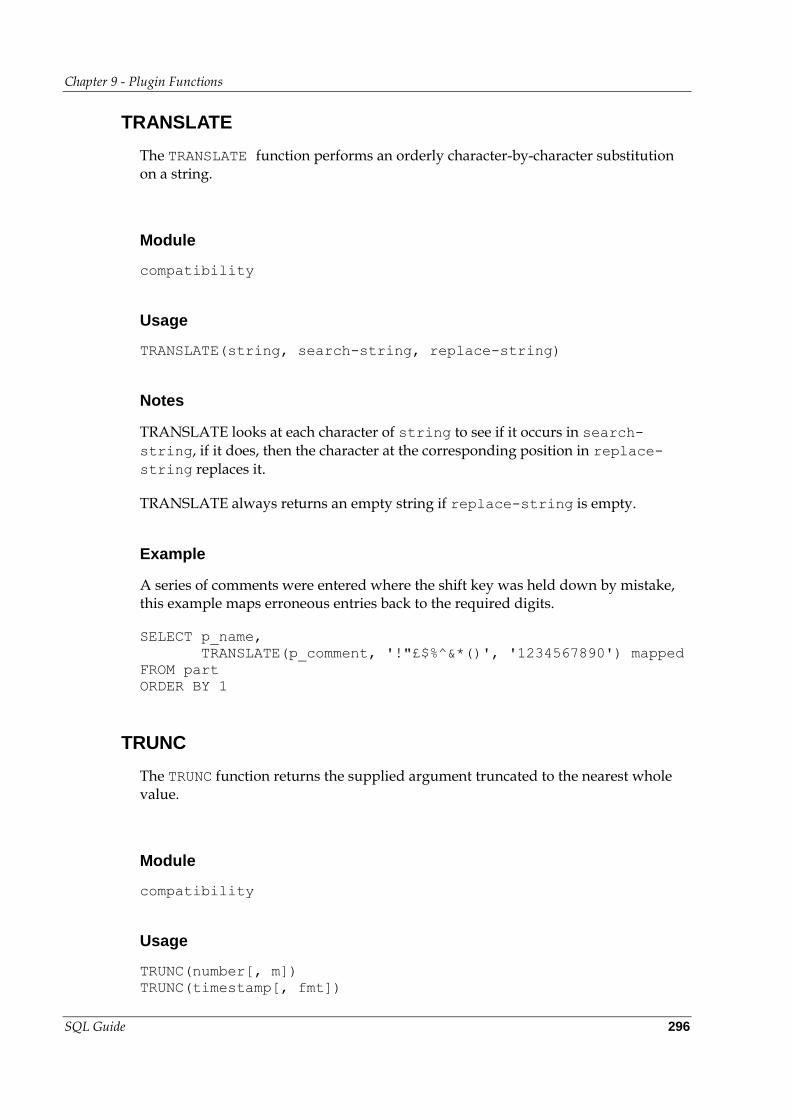
Chapter 9 - Plugin Functions
SQL Guide 296
TRANSLATE
The TRANSLATE function performs an orderly character-by-character substitution on a string.
Module
compatibility
Usage
TRANSLATE(string, search-string, replace-string)
Notes
TRANSLATE looks at each character of string to see if it occurs in search-string, if it does, then the character at the corresponding position in replace-string replaces it.
TRANSLATE always returns an empty string if replace-string is empty.
Example
A series of comments were entered where the shift key was held down by mistake, this example maps erroneous entries back to the required digits.
SELECT p_name,
TRANSLATE(p_comment, '!"£$%^&*()', '1234567890') mapped
FROM part
ORDER BY 1
TRUNC
The TRUNC function returns the supplied argument truncated to the nearest whole value.
Module
compatibility
Usage
TRUNC(number[, m])
TRUNC(timestamp[, fmt])
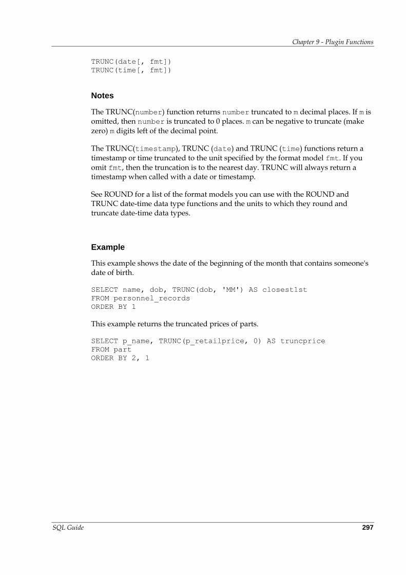
Chapter 9 - Plugin Functions
SQL Guide 297
TRUNC(date[, fmt])
TRUNC(time[, fmt])
Notes
The TRUNC(number) function returns number truncated to m decimal places. If m is omitted, then number is truncated to 0 places. m can be negative to truncate (make zero) m digits left of the decimal point.
The TRUNC(timestamp), TRUNC (date) and TRUNC (time) functions return a timestamp or time truncated to the unit specified by the format model fmt. If you
omit fmt, then the truncation is to the nearest day. TRUNC will always return a timestamp when called with a date or timestamp.
See ROUND for a list of the format models you can use with the ROUND and TRUNC date-time data type functions and the units to which they round and truncate date-time data types.
Example
This example shows the date of the beginning of the month that contains someone's date of birth.
SELECT name, dob, TRUNC(dob, 'MM') AS closest1st
FROM personnel_records
ORDER BY 1
This example returns the truncated prices of parts.
SELECT p_name, TRUNC(p_retailprice, 0) AS truncprice
FROM part
ORDER BY 2, 1

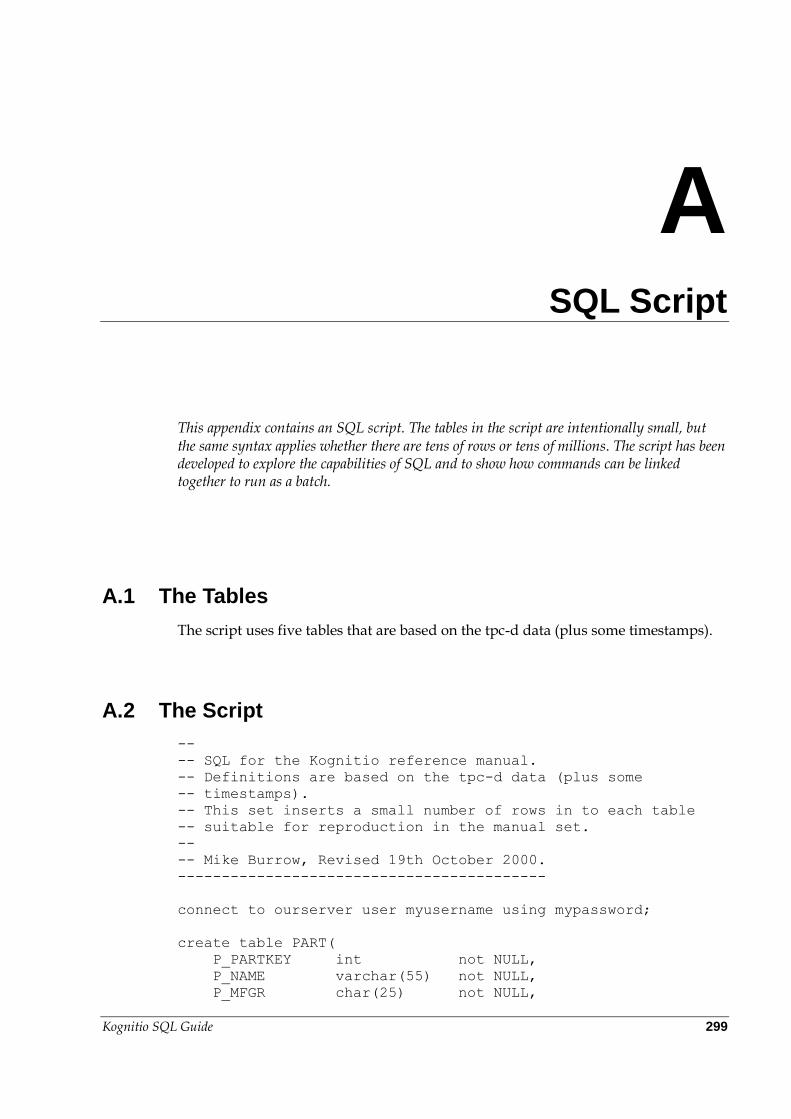
Kognitio SQL Guide 299
A
SQL Script
This appendix contains an SQL script. The tables in the script are intentionally small, but the same syntax applies whether there are tens of rows or tens of millions. The script has been developed to explore the capabilities of SQL and to show how commands can be linked together to run as a batch.
A.1 The Tables
The script uses five tables that are based on the tpc-d data (plus some timestamps).
A.2 The Script
--
-- SQL for the Kognitio reference manual.
-- Definitions are based on the tpc-d data (plus some
-- timestamps).
-- This set inserts a small number of rows in to each table
-- suitable for reproduction in the manual set.
--
-- Mike Burrow, Revised 19th October 2000.
------------------------------------------
connect to ourserver user myusername using mypassword;
create table PART(
P_PARTKEY int not NULL,
P_NAME varchar(55) not NULL,
P_MFGR char(25) not NULL,
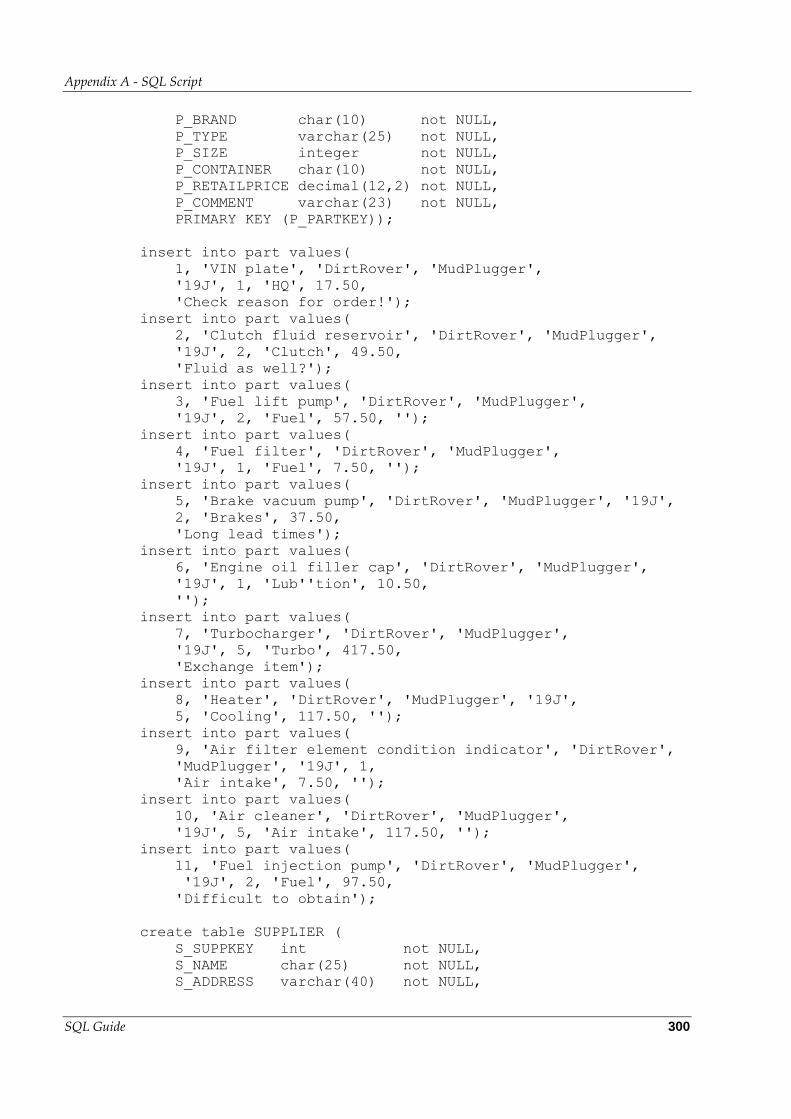
Appendix A - SQL Script
SQL Guide 300
P_BRAND char(10) not NULL,
P_TYPE varchar(25) not NULL,
P_SIZE integer not NULL,
P_CONTAINER char(10) not NULL,
P_RETAILPRICE decimal(12,2) not NULL,
P_COMMENT varchar(23) not NULL,
PRIMARY KEY (P_PARTKEY));
insert into part values(
1, 'VIN plate', 'DirtRover', 'MudPlugger',
'19J', 1, 'HQ', 17.50,
'Check reason for order!');
insert into part values(
2, 'Clutch fluid reservoir', 'DirtRover', 'MudPlugger',
'19J', 2, 'Clutch', 49.50,
'Fluid as well?');
insert into part values(
3, 'Fuel lift pump', 'DirtRover', 'MudPlugger',
'19J', 2, 'Fuel', 57.50, '');
insert into part values(
4, 'Fuel filter', 'DirtRover', 'MudPlugger',
'19J', 1, 'Fuel', 7.50, '');
insert into part values(
5, 'Brake vacuum pump', 'DirtRover', 'MudPlugger', '19J',
2, 'Brakes', 37.50,
'Long lead times');
insert into part values(
6, 'Engine oil filler cap', 'DirtRover', 'MudPlugger',
'19J', 1, 'Lub''tion', 10.50,
'');
insert into part values(
7, 'Turbocharger', 'DirtRover', 'MudPlugger',
'19J', 5, 'Turbo', 417.50,
'Exchange item');
insert into part values(
8, 'Heater', 'DirtRover', 'MudPlugger', '19J',
5, 'Cooling', 117.50, '');
insert into part values(
9, 'Air filter element condition indicator', 'DirtRover',
'MudPlugger', '19J', 1,
'Air intake', 7.50, '');
insert into part values(
10, 'Air cleaner', 'DirtRover', 'MudPlugger',
'19J', 5, 'Air intake', 117.50, '');
insert into part values(
11, 'Fuel injection pump', 'DirtRover', 'MudPlugger',
'19J', 2, 'Fuel', 97.50,
'Difficult to obtain');
create table SUPPLIER (
S_SUPPKEY int not NULL,
S_NAME char(25) not NULL,
S_ADDRESS varchar(40) not NULL,
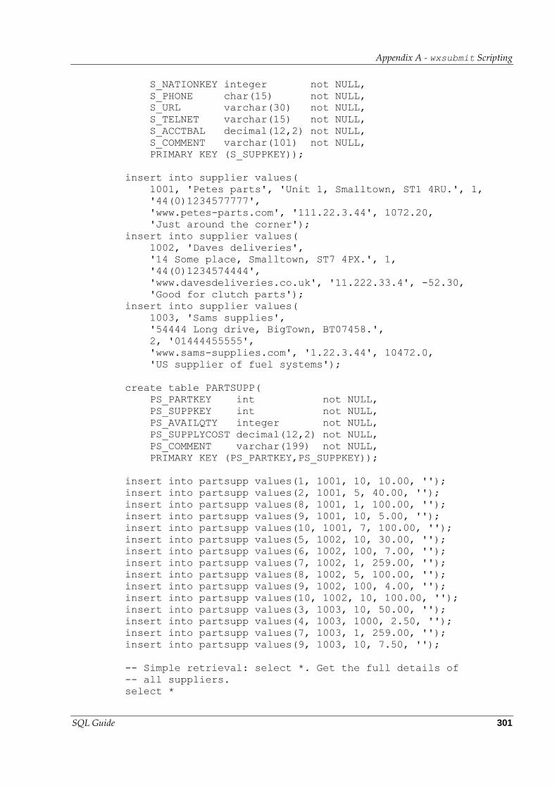
Appendix A - wxsubmit Scripting
SQL Guide 301
S_NATIONKEY integer not NULL,
S_PHONE char(15) not NULL,
S_URL varchar(30) not NULL,
S_TELNET varchar(15) not NULL,
S_ACCTBAL decimal(12,2) not NULL,
S_COMMENT varchar(101) not NULL,
PRIMARY KEY (S_SUPPKEY));
insert into supplier values(
1001, 'Petes parts', 'Unit 1, Smalltown, ST1 4RU.', 1,
'44(0)1234577777',
'www.petes-parts.com', '111.22.3.44', 1072.20,
'Just around the corner');
insert into supplier values(
1002, 'Daves deliveries',
'14 Some place, Smalltown, ST7 4PX.', 1,
'44(0)1234574444',
'www.davesdeliveries.co.uk', '11.222.33.4', -52.30,
'Good for clutch parts');
insert into supplier values(
1003, 'Sams supplies',
'54444 Long drive, BigTown, BT07458.',
2, '01444455555',
'www.sams-supplies.com', '1.22.3.44', 10472.0,
'US supplier of fuel systems');
create table PARTSUPP(
PS_PARTKEY int not NULL,
PS_SUPPKEY int not NULL,
PS_AVAILQTY integer not NULL,
PS_SUPPLYCOST decimal(12,2) not NULL,
PS_COMMENT varchar(199) not NULL,
PRIMARY KEY (PS_PARTKEY,PS_SUPPKEY));
insert into partsupp values(1, 1001, 10, 10.00, '');
insert into partsupp values(2, 1001, 5, 40.00, '');
insert into partsupp values(8, 1001, 1, 100.00, '');
insert into partsupp values(9, 1001, 10, 5.00, '');
insert into partsupp values(10, 1001, 7, 100.00, '');
insert into partsupp values(5, 1002, 10, 30.00, '');
insert into partsupp values(6, 1002, 100, 7.00, '');
insert into partsupp values(7, 1002, 1, 259.00, '');
insert into partsupp values(8, 1002, 5, 100.00, '');
insert into partsupp values(9, 1002, 100, 4.00, '');
insert into partsupp values(10, 1002, 10, 100.00, '');
insert into partsupp values(3, 1003, 10, 50.00, '');
insert into partsupp values(4, 1003, 1000, 2.50, '');
insert into partsupp values(7, 1003, 1, 259.00, '');
insert into partsupp values(9, 1003, 10, 7.50, '');
-- Simple retrieval: select *. Get the full details of
-- all suppliers.
select *
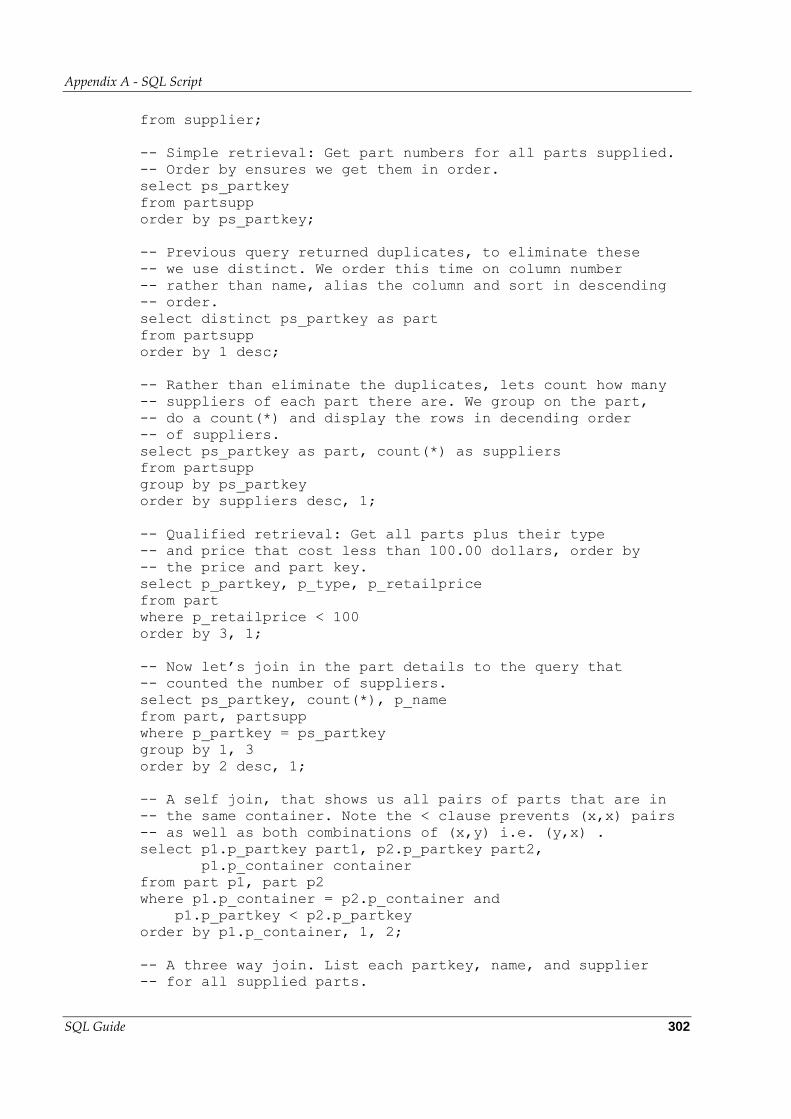
Appendix A - SQL Script
SQL Guide 302
from supplier;
-- Simple retrieval: Get part numbers for all parts supplied.
-- Order by ensures we get them in order.
select ps_partkey
from partsupp
order by ps_partkey;
-- Previous query returned duplicates, to eliminate these
-- we use distinct. We order this time on column number
-- rather than name, alias the column and sort in descending
-- order.
select distinct ps_partkey as part
from partsupp
order by 1 desc;
-- Rather than eliminate the duplicates, lets count how many
-- suppliers of each part there are. We group on the part,
-- do a count(*) and display the rows in decending order
-- of suppliers.
select ps_partkey as part, count(*) as suppliers
from partsupp
group by ps_partkey
order by suppliers desc, 1;
-- Qualified retrieval: Get all parts plus their type
-- and price that cost less than 100.00 dollars, order by
-- the price and part key.
select p_partkey, p_type, p_retailprice
from part
where p_retailprice < 100
order by 3, 1;
-- Now let’s join in the part details to the query that
-- counted the number of suppliers.
select ps_partkey, count(*), p_name
from part, partsupp
where p_partkey = ps_partkey
group by 1, 3
order by 2 desc, 1;
-- A self join, that shows us all pairs of parts that are in
-- the same container. Note the < clause prevents (x,x) pairs
-- as well as both combinations of (x,y) i.e. (y,x) .
select p1.p_partkey part1, p2.p_partkey part2,
p1.p_container container
from part p1, part p2
where p1.p_container = p2.p_container and
p1.p_partkey < p2.p_partkey
order by p1.p_container, 1, 2;
-- A three way join. List each partkey, name, and supplier
-- for all supplied parts.
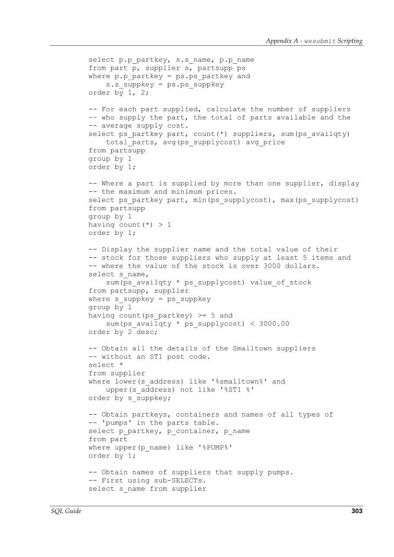
Appendix A - wxsubmit Scripting
SQL Guide 303
select p.p_partkey, s.s_name, p.p_name
from part p, supplier s, partsupp ps
where p.p_partkey = ps.ps_partkey and
s.s_suppkey = ps.ps_suppkey
order by 1, 2;
-- For each part supplied, calculate the number of suppliers
-- who supply the part, the total of parts available and the
-- average supply cost.
select ps_partkey part, count(*) suppliers, sum(ps_availqty)
total_parts, avg(ps_supplycost) avg_price
from partsupp
group by 1
order by 1;
-- Where a part is supplied by more than one supplier, display
-- the maximum and minimum prices.
select ps_partkey part, min(ps_supplycost), max(ps_supplycost)
from partsupp
group by 1
having count(*) > 1
order by 1;
-- Display the supplier name and the total value of their
-- stock for those suppliers who supply at least 5 items and
-- where the value of the stock is over 3000 dollars.
select s_name,
sum(ps_availqty * ps_supplycost) value_of_stock
from partsupp, supplier
where s_suppkey = ps_suppkey
group by 1
having count(ps_partkey) >= 5 and
sum(ps_availqty * ps_supplycost) < 3000.00
order by 2 desc;
-- Obtain all the details of the Smalltown suppliers
-- without an ST1 post code.
select *
from supplier
where lower(s_address) like '%smalltown%' and
upper(s_address) not like '%ST1 %'
order by s_suppkey;
-- Obtain partkeys, containers and names of all types of
-- 'pumps' in the parts table.
select p_partkey, p_container, p_name
from part
where upper(p_name) like '%PUMP%'
order by 1;
-- Obtain names of suppliers that supply pumps.
-- First using sub-SELECTs.
select s_name from supplier
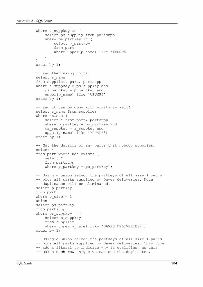
Appendix A - SQL Script
SQL Guide 304
where s_suppkey in (
select ps_suppkey from partsupp
where ps_partkey in (
select p_partkey
from part
where upper(p_name) like '%PUMP%'
)
)
order by 1;
-- and then using joins.
select s_name
from supplier, part, partsupp
where s_suppkey = ps_suppkey and
ps_partkey = p_partkey and
upper(p_name) like '%PUMP%'
order by 1;
-- and it can be done with exists as well!
select s_name from supplier
where exists (
select * from part, partsupp
where p_partkey = ps_partkey and
ps_suppkey = s_suppkey and
upper(p_name) like '%PUMP%')
order by 1;
-- Get the details of any parts that nobody supplies.
select *
from part where not exists (
select *
from partsupp
where p_partkey = ps_partkey);
-- Using a union select the partkeys of all size 1 parts
-- plus all parts supplied by Daves deliveries. Note
-- duplicates will be eliminated.
select p_partkey
from part
where p_size = 1
union
select ps_partkey
from partsupp
where ps_suppkey = (
select s_suppkey
from supplier
where upper(s_name) like 'DAVES DELIVERIES%')
order by 1;
-- Using a union select the partkeys of all size 1 parts
-- plus all parts supplied by Daves deliveries. This time
-- add a literal to indicate why it qualifies, as this
-- makes each row unique we can see the duplicates.
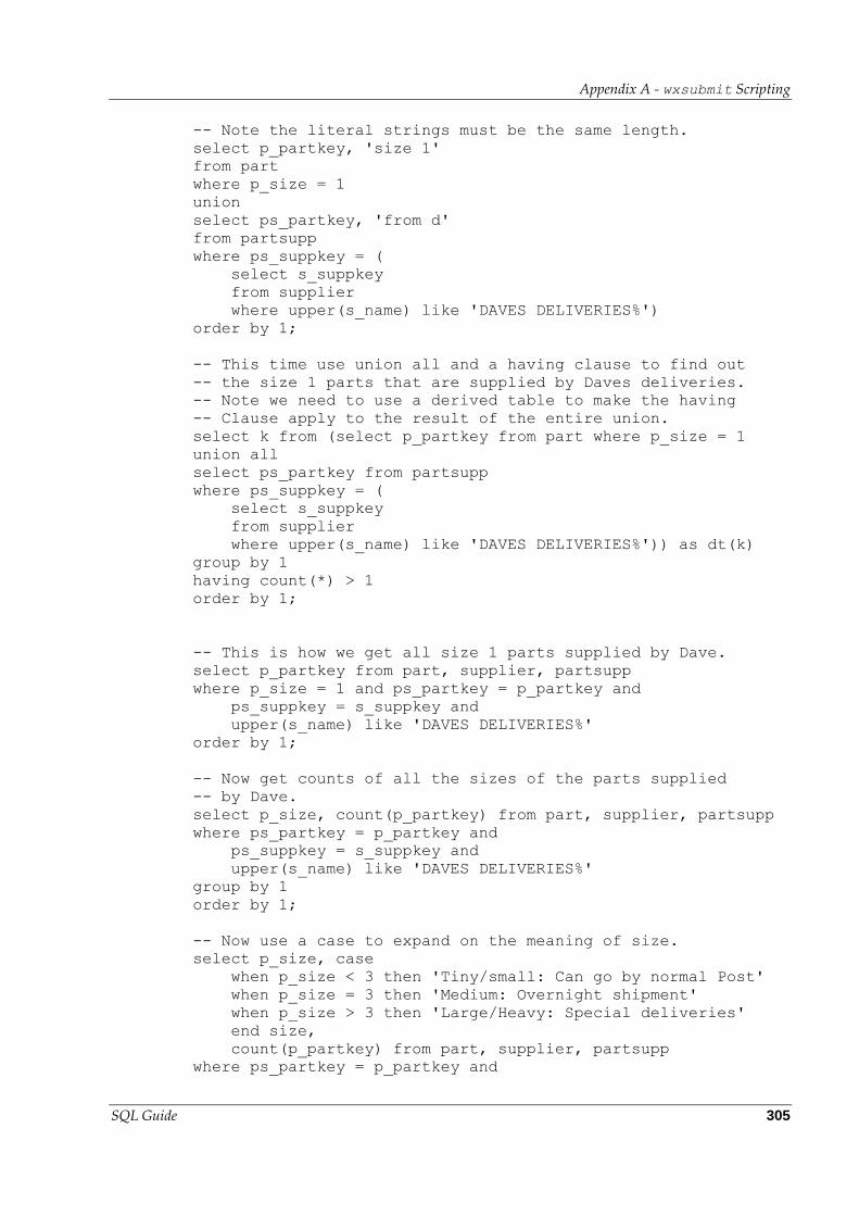
Appendix A - wxsubmit Scripting
SQL Guide 305
-- Note the literal strings must be the same length.
select p_partkey, 'size 1'
from part
where p_size = 1
union
select ps_partkey, 'from d'
from partsupp
where ps_suppkey = (
select s_suppkey
from supplier
where upper(s_name) like 'DAVES DELIVERIES%')
order by 1;
-- This time use union all and a having clause to find out
-- the size 1 parts that are supplied by Daves deliveries.
-- Note we need to use a derived table to make the having
-- Clause apply to the result of the entire union.
select k from (select p_partkey from part where p_size = 1
union all
select ps_partkey from partsupp
where ps_suppkey = (
select s_suppkey
from supplier
where upper(s_name) like 'DAVES DELIVERIES%')) as dt(k)
group by 1
having count(*) > 1
order by 1;
-- This is how we get all size 1 parts supplied by Dave.
select p_partkey from part, supplier, partsupp
where p_size = 1 and ps_partkey = p_partkey and
ps_suppkey = s_suppkey and
upper(s_name) like 'DAVES DELIVERIES%'
order by 1;
-- Now get counts of all the sizes of the parts supplied
-- by Dave.
select p_size, count(p_partkey) from part, supplier, partsupp
where ps_partkey = p_partkey and
ps_suppkey = s_suppkey and
upper(s_name) like 'DAVES DELIVERIES%'
group by 1
order by 1;
-- Now use a case to expand on the meaning of size.
select p_size, case
when p_size < 3 then 'Tiny/small: Can go by normal Post'
when p_size = 3 then 'Medium: Overnight shipment'
when p_size > 3 then 'Large/Heavy: Special deliveries'
end size,
count(p_partkey) from part, supplier, partsupp
where ps_partkey = p_partkey and
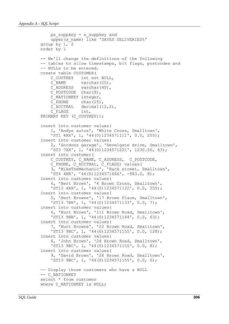
Appendix A - SQL Script
SQL Guide 306
ps_suppkey = s_suppkey and
upper(s_name) like 'DAVES DELIVERIES%'
group by 1, 2
order by 1
-- We'll change the definitions of the following
-- tables to allow timestamps, bit flags, postcodes and
-- NULLs to be entered.
create table CUSTOMER(
C_CUSTKEY int not NULL,
C_NAME varchar(25),
C_ADDRESS varchar(40),
C_POSTCODE char(9),
C_NATIONKEY integer,
C_PHONE char(15),
C_ACCTBAL decimal(12,2),
C_FLAGS int,
PRIMARY KEY (C_CUSTKEY));
insert into customer values(
1, 'Andys autos', 'White Cross, Smalltown',
'ST1 4RX', 1, '44(0)1234571111', 0.0, 255);
insert into customer values(
2, 'Gordons garage', 'Develgate drive, Smalltown',
'ST3 7XX', 1, '44(0)1234571221', 1230.50, 63);
insert into customer(
C_CUSTKEY, C_NAME, C_ADDRESS, C_POSTCODE,
C_PHONE, C_ACCTBAL, C_FLAGS) values(
3, 'MikeTheMechanic', 'Back street, Smalltown',
'ST4 4RR', '44(0)1234571666', -983.0, 8);
insert into customer values(
4, 'Bert Brown', '4 Brown Cross, Smalltown',
'ST13 4RX', 1, '44(0)1234571122', 0.0, 255);
insert into customer values(
5, 'Bert Browne', '17 Brown Place, Smalltown',
'ST13 7BN', 1, '44(0)1234571133', 0.0, 7);
insert into customer values(
6, 'Burt Brown', '111 Brown Road, Smalltown',
'ST13 9BB', 1, '44(0)1234571144', 0.0, 63);
insert into customer values(
7, 'Burt Browne', '22 Brown Road, Smalltown',
'ST13 9BC', 1, '44(0)1234571155', 0.0, 128);
insert into customer values(
8, 'John Brown', '24 Brown Road, Smalltown',
'ST13 9BC', 1, '44(0)1234571155', 0.0, 8);
insert into customer values(
9, 'David Brown', '26 Brown Road, Smalltown',
'ST13 9BC', 1, '44(0)1234571155', 0.0, 0);
-- Display those customers who have a NULL
-- C_NATIONKEY
select * from customer
where C_NATIONKEY is NULL;
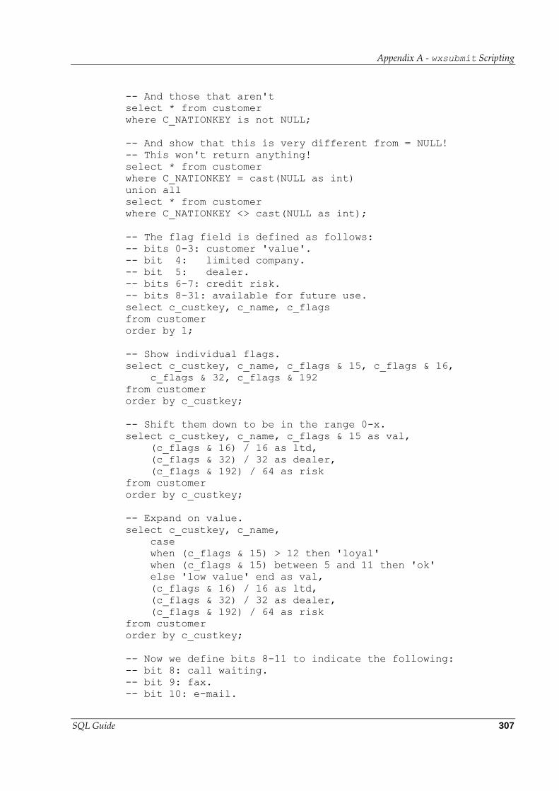
Appendix A - wxsubmit Scripting
SQL Guide 307
-- And those that aren't
select * from customer
where C_NATIONKEY is not NULL;
-- And show that this is very different from = NULL!
-- This won't return anything!
select * from customer
where C_NATIONKEY = cast(NULL as int)
union all
select * from customer
where C_NATIONKEY <> cast(NULL as int);
-- The flag field is defined as follows:
-- bits 0-3: customer 'value'.
-- bit 4: limited company.
-- bit 5: dealer.
-- bits 6-7: credit risk.
-- bits 8-31: available for future use.
select c_custkey, c_name, c_flags
from customer
order by 1;
-- Show individual flags.
select c_custkey, c_name, c_flags & 15, c_flags & 16,
c_flags & 32, c_flags & 192
from customer
order by c_custkey;
-- Shift them down to be in the range 0-x.
select c_custkey, c_name, c_flags & 15 as val,
(c_flags & 16) / 16 as ltd,
(c_flags & 32) / 32 as dealer,
(c_flags & 192) / 64 as risk
from customer
order by c_custkey;
-- Expand on value.
select c_custkey, c_name,
case
when (c_flags & 15) > 12 then 'loyal'
when (c_flags & 15) between 5 and 11 then 'ok'
else 'low value' end as val,
(c_flags & 16) / 16 as ltd,
(c_flags & 32) / 32 as dealer,
(c_flags & 192) / 64 as risk
from customer
order by c_custkey;
-- Now we define bits 8-11 to indicate the following:
-- bit 8: call waiting.
-- bit 9: fax.
-- bit 10: e-mail.
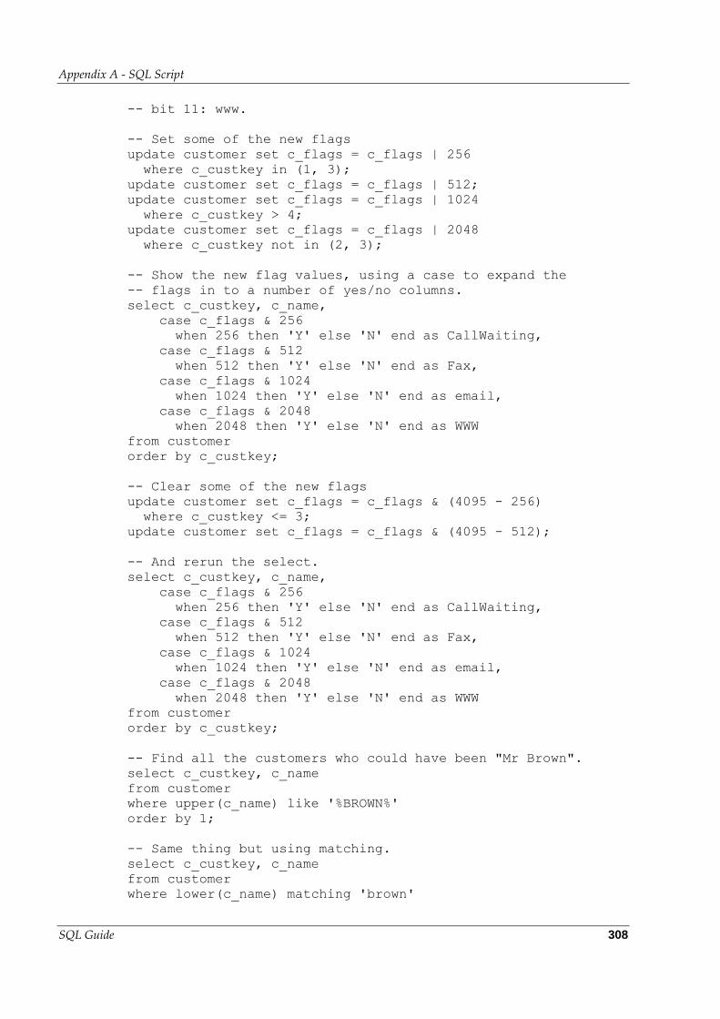
Appendix A - SQL Script
SQL Guide 308
-- bit 11: www.
-- Set some of the new flags
update customer set c_flags = c_flags | 256
where c_custkey in (1, 3);
update customer set c_flags = c_flags | 512;
update customer set c_flags = c_flags | 1024
where c_custkey > 4;
update customer set c_flags = c_flags | 2048
where c_custkey not in (2, 3);
-- Show the new flag values, using a case to expand the
-- flags in to a number of yes/no columns.
select c_custkey, c_name,
case c_flags & 256
when 256 then 'Y' else 'N' end as CallWaiting,
case c_flags & 512
when 512 then 'Y' else 'N' end as Fax,
case c_flags & 1024
when 1024 then 'Y' else 'N' end as email,
case c_flags & 2048
when 2048 then 'Y' else 'N' end as WWW
from customer
order by c_custkey;
-- Clear some of the new flags
update customer set c_flags = c_flags & (4095 - 256)
where c_custkey <= 3;
update customer set c_flags = c_flags & (4095 - 512);
-- And rerun the select.
select c_custkey, c_name,
case c_flags & 256
when 256 then 'Y' else 'N' end as CallWaiting,
case c_flags & 512
when 512 then 'Y' else 'N' end as Fax,
case c_flags & 1024
when 1024 then 'Y' else 'N' end as email,
case c_flags & 2048
when 2048 then 'Y' else 'N' end as WWW
from customer
order by c_custkey;
-- Find all the customers who could have been "Mr Brown".
select c_custkey, c_name
from customer
where upper(c_name) like '%BROWN%'
order by 1;
-- Same thing but using matching.
select c_custkey, c_name
from customer
where lower(c_name) matching 'brown'
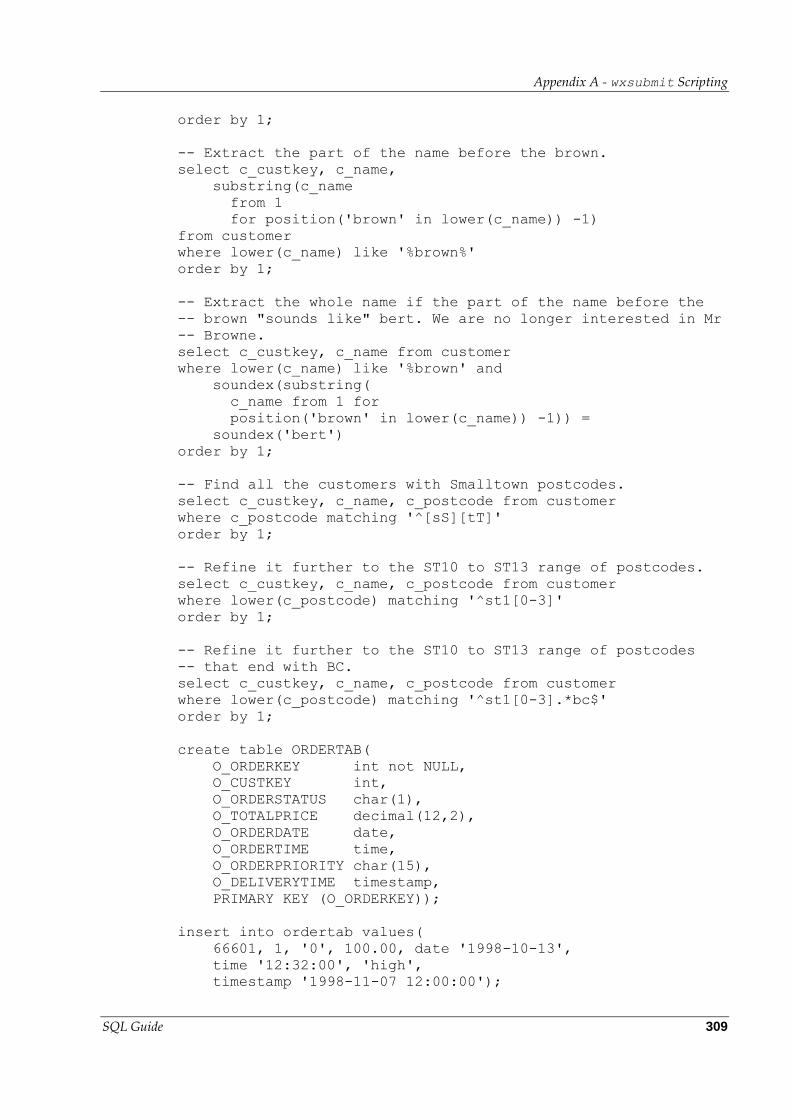
Appendix A - wxsubmit Scripting
SQL Guide 309
order by 1;
-- Extract the part of the name before the brown.
select c_custkey, c_name,
substring(c_name
from 1
for position('brown' in lower(c_name)) -1)
from customer
where lower(c_name) like '%brown%'
order by 1;
-- Extract the whole name if the part of the name before the
-- brown "sounds like" bert. We are no longer interested in Mr
-- Browne.
select c_custkey, c_name from customer
where lower(c_name) like '%brown' and
soundex(substring(
c_name from 1 for
position('brown' in lower(c_name)) -1)) =
soundex('bert')
order by 1;
-- Find all the customers with Smalltown postcodes.
select c_custkey, c_name, c_postcode from customer
where c_postcode matching '^[sS][tT]'
order by 1;
-- Refine it further to the ST10 to ST13 range of postcodes.
select c_custkey, c_name, c_postcode from customer
where lower(c_postcode) matching '^st1[0-3]'
order by 1;
-- Refine it further to the ST10 to ST13 range of postcodes
-- that end with BC.
select c_custkey, c_name, c_postcode from customer
where lower(c_postcode) matching '^st1[0-3].*bc$'
order by 1;
create table ORDERTAB(
O_ORDERKEY int not NULL,
O_CUSTKEY int,
O_ORDERSTATUS char(1),
O_TOTALPRICE decimal(12,2),
O_ORDERDATE date,
O_ORDERTIME time,
O_ORDERPRIORITY char(15),
O_DELIVERYTIME timestamp,
PRIMARY KEY (O_ORDERKEY));
insert into ordertab values(
66601, 1, '0', 100.00, date '1998-10-13',
time '12:32:00', 'high',
timestamp '1998-11-07 12:00:00');
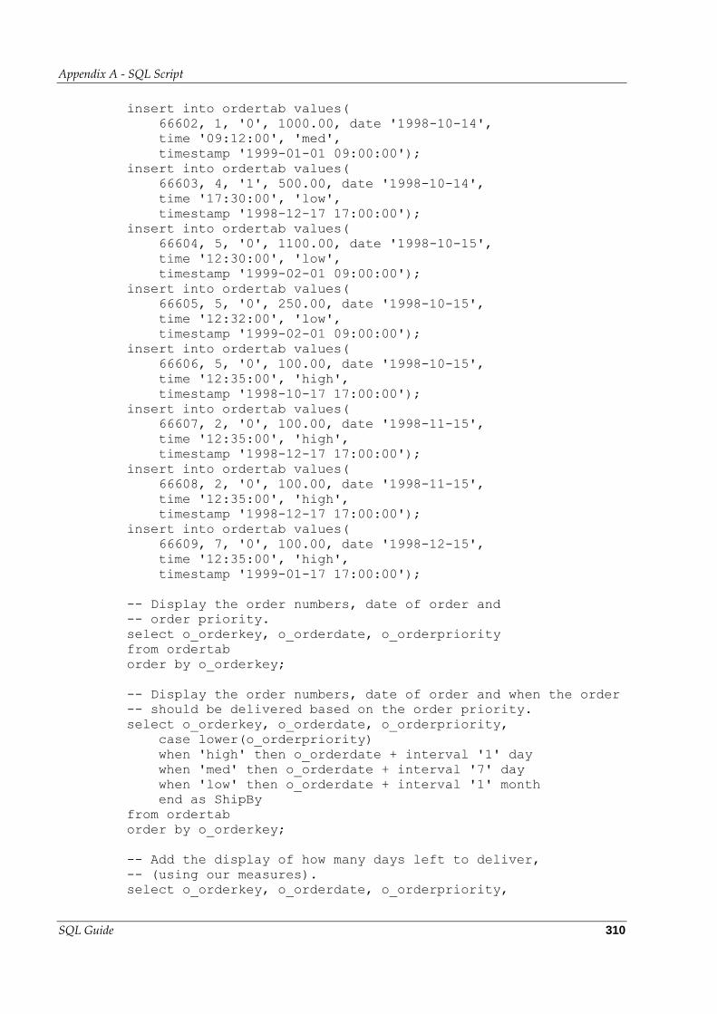
Appendix A - SQL Script
SQL Guide 310
insert into ordertab values(
66602, 1, '0', 1000.00, date '1998-10-14',
time '09:12:00', 'med',
timestamp '1999-01-01 09:00:00');
insert into ordertab values(
66603, 4, '1', 500.00, date '1998-10-14',
time '17:30:00', 'low',
timestamp '1998-12-17 17:00:00');
insert into ordertab values(
66604, 5, '0', 1100.00, date '1998-10-15',
time '12:30:00', 'low',
timestamp '1999-02-01 09:00:00');
insert into ordertab values(
66605, 5, '0', 250.00, date '1998-10-15',
time '12:32:00', 'low',
timestamp '1999-02-01 09:00:00');
insert into ordertab values(
66606, 5, '0', 100.00, date '1998-10-15',
time '12:35:00', 'high',
timestamp '1998-10-17 17:00:00');
insert into ordertab values(
66607, 2, '0', 100.00, date '1998-11-15',
time '12:35:00', 'high',
timestamp '1998-12-17 17:00:00');
insert into ordertab values(
66608, 2, '0', 100.00, date '1998-11-15',
time '12:35:00', 'high',
timestamp '1998-12-17 17:00:00');
insert into ordertab values(
66609, 7, '0', 100.00, date '1998-12-15',
time '12:35:00', 'high',
timestamp '1999-01-17 17:00:00');
-- Display the order numbers, date of order and
-- order priority.
select o_orderkey, o_orderdate, o_orderpriority
from ordertab
order by o_orderkey;
-- Display the order numbers, date of order and when the order
-- should be delivered based on the order priority.
select o_orderkey, o_orderdate, o_orderpriority,
case lower(o_orderpriority)
when 'high' then o_orderdate + interval '1' day
when 'med' then o_orderdate + interval '7' day
when 'low' then o_orderdate + interval '1' month
end as ShipBy
from ordertab
order by o_orderkey;
-- Add the display of how many days left to deliver,
-- (using our measures).
select o_orderkey, o_orderdate, o_orderpriority,
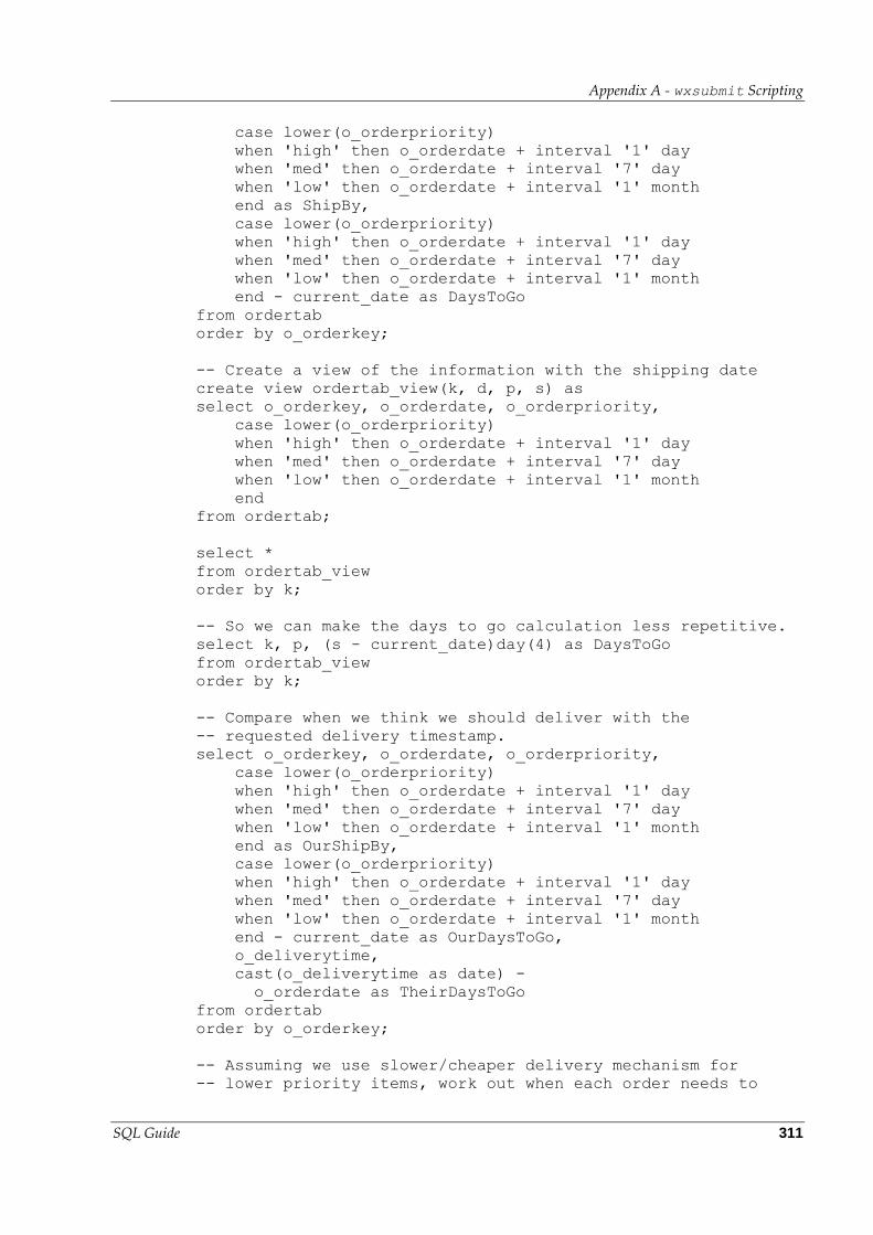
Appendix A - wxsubmit Scripting
SQL Guide 311
case lower(o_orderpriority)
when 'high' then o_orderdate + interval '1' day
when 'med' then o_orderdate + interval '7' day
when 'low' then o_orderdate + interval '1' month
end as ShipBy,
case lower(o_orderpriority)
when 'high' then o_orderdate + interval '1' day
when 'med' then o_orderdate + interval '7' day
when 'low' then o_orderdate + interval '1' month
end - current_date as DaysToGo
from ordertab
order by o_orderkey;
-- Create a view of the information with the shipping date
create view ordertab_view(k, d, p, s) as
select o_orderkey, o_orderdate, o_orderpriority,
case lower(o_orderpriority)
when 'high' then o_orderdate + interval '1' day
when 'med' then o_orderdate + interval '7' day
when 'low' then o_orderdate + interval '1' month
end
from ordertab;
select *
from ordertab_view
order by k;
-- So we can make the days to go calculation less repetitive.
select k, p, (s - current_date)day(4) as DaysToGo
from ordertab_view
order by k;
-- Compare when we think we should deliver with the
-- requested delivery timestamp.
select o_orderkey, o_orderdate, o_orderpriority,
case lower(o_orderpriority)
when 'high' then o_orderdate + interval '1' day
when 'med' then o_orderdate + interval '7' day
when 'low' then o_orderdate + interval '1' month
end as OurShipBy,
case lower(o_orderpriority)
when 'high' then o_orderdate + interval '1' day
when 'med' then o_orderdate + interval '7' day
when 'low' then o_orderdate + interval '1' month
end - current_date as OurDaysToGo,
o_deliverytime,
cast(o_deliverytime as date) -
o_orderdate as TheirDaysToGo
from ordertab
order by o_orderkey;
-- Assuming we use slower/cheaper delivery mechanism for
-- lower priority items, work out when each order needs to
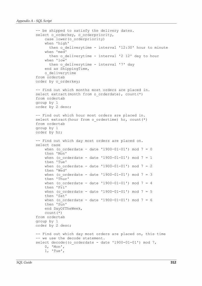
Appendix A - SQL Script
SQL Guide 312
-- be shipped to satisfy the delivery dates.
select o_orderkey, o_orderpriority,
case lower(o_orderpriority)
when 'high'
then o_deliverytime - interval '12:30' hour to minute
when 'med'
then o_deliverytime - interval '2 12' day to hour
when 'low'
then o_deliverytime - interval '7' day
end as ShippingTime,
o_deliverytime
from ordertab
order by o_orderkey;
-- Find out which months most orders are placed in.
select extract(month from o_orderdate), count(*)
from ordertab
group by 1
order by 2 desc;
-- Find out which hour most orders are placed in.
select extract(hour from o_ordertime) hr, count(*)
from ordertab
group by 1
order by hr;
-- Find out which day most orders are placed on.
select case
when (o_orderdate - date '1900-01-01') mod 7 = 0
then 'Mon'
when (o_orderdate - date '1900-01-01') mod 7 = 1
then 'Tue'
when (o_orderdate - date '1900-01-01') mod 7 = 2
then 'Wed'
when (o_orderdate - date '1900-01-01') mod 7 = 3
then 'Thur'
when (o_orderdate - date '1900-01-01') mod 7 = 4
then 'Fri'
when (o_orderdate - date '1900-01-01') mod 7 = 5
then 'Sat'
when (o_orderdate - date '1900-01-01') mod 7 = 6
then 'Sun'
end DayOfTheWeek,
count(*)
from ordertab
group by 1
order by 2 desc;
-- Find out which day most orders are placed on, this time
-- we use the decode statement.
select decode((o_orderdate - date '1900-01-01') mod 7,
0, 'Mon',
1, 'Tue',
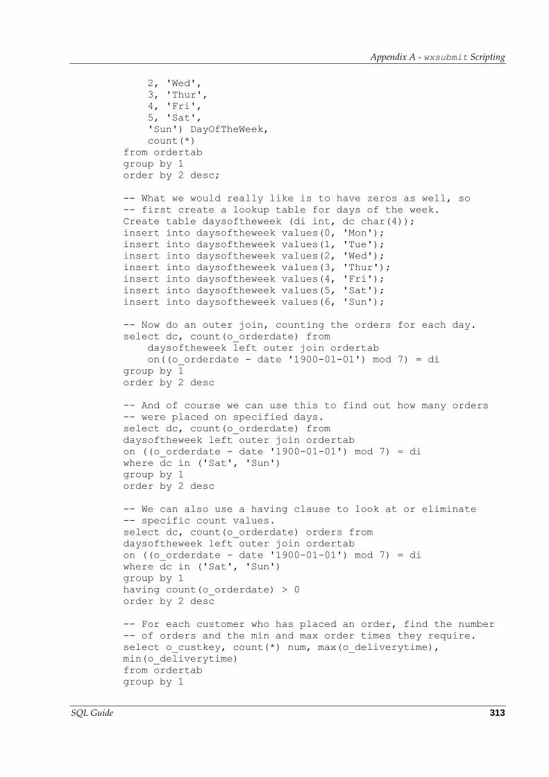
Appendix A - wxsubmit Scripting
SQL Guide 313
2, 'Wed',
3, 'Thur',
4, 'Fri',
5, 'Sat',
'Sun') DayOfTheWeek,
count(*)
from ordertab
group by 1
order by 2 desc;
-- What we would really like is to have zeros as well, so
-- first create a lookup table for days of the week.
Create table daysoftheweek (di int, dc char(4));
insert into daysoftheweek values(0, 'Mon');
insert into daysoftheweek values(1, 'Tue');
insert into daysoftheweek values(2, 'Wed');
insert into daysoftheweek values(3, 'Thur');
insert into daysoftheweek values(4, 'Fri');
insert into daysoftheweek values(5, 'Sat');
insert into daysoftheweek values(6, 'Sun');
-- Now do an outer join, counting the orders for each day.
select dc, count(o_orderdate) from
daysoftheweek left outer join ordertab
on((o_orderdate - date '1900-01-01') mod 7) = di
group by 1
order by 2 desc
-- And of course we can use this to find out how many orders
-- were placed on specified days.
select dc, count(o_orderdate) from
daysoftheweek left outer join ordertab
on ((o_orderdate - date '1900-01-01') mod 7) = di
where dc in ('Sat', 'Sun')
group by 1
order by 2 desc
-- We can also use a having clause to look at or eliminate
-- specific count values.
select dc, count(o_orderdate) orders from
daysoftheweek left outer join ordertab
on ((o_orderdate - date '1900-01-01') mod 7) = di
where dc in ('Sat', 'Sun')
group by 1
having count(o_orderdate) > 0
order by 2 desc
-- For each customer who has placed an order, find the number
-- of orders and the min and max order times they require.
select o_custkey, count(*) num, max(o_deliverytime),
min(o_deliverytime)
from ordertab
group by 1
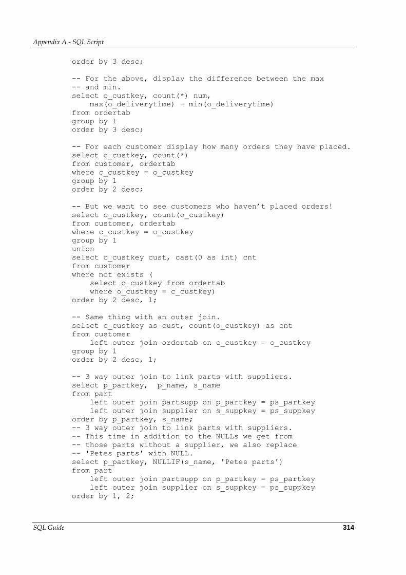
Appendix A - SQL Script
SQL Guide 314
order by 3 desc;
-- For the above, display the difference between the max
-- and min.
select o_custkey, count(*) num,
max(o_deliverytime) - min(o_deliverytime)
from ordertab
group by 1
order by 3 desc;
-- For each customer display how many orders they have placed.
select c_custkey, count(*)
from customer, ordertab
where c_custkey = o_custkey
group by 1
order by 2 desc;
-- But we want to see customers who haven’t placed orders!
select c_custkey, count(o_custkey)
from customer, ordertab
where c_custkey = o_custkey
group by 1
union
select c_custkey cust, cast(0 as int) cnt
from customer
where not exists (
select o_custkey from ordertab
where o_custkey = c_custkey)
order by 2 desc, 1;
-- Same thing with an outer join.
select c_custkey as cust, count(o_custkey) as cnt
from customer
left outer join ordertab on c_custkey = o_custkey
group by 1
order by 2 desc, 1;
-- 3 way outer join to link parts with suppliers.
select p_partkey, p_name, s_name
from part
left outer join partsupp on p_partkey = ps_partkey
left outer join supplier on s_suppkey = ps_suppkey
order by p_partkey, s_name;
-- 3 way outer join to link parts with suppliers.
-- This time in addition to the NULLs we get from
-- those parts without a supplier, we also replace
-- 'Petes parts' with NULL.
select p_partkey, NULLIF(s_name, 'Petes parts')
from part
left outer join partsupp on p_partkey = ps_partkey
left outer join supplier on s_suppkey = ps_suppkey
order by 1, 2;
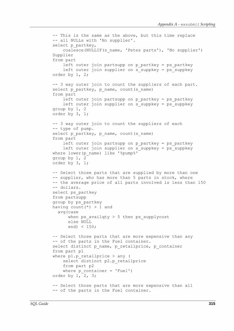
Appendix A - wxsubmit Scripting
SQL Guide 315
-- This is the same as the above, but this time replace
-- all NULLs with 'No supplier'.
select p_partkey,
coalesce(NULLIF(s_name, 'Petes parts'), 'No supplier')
Supplier
from part
left outer join partsupp on p_partkey = ps_partkey
left outer join supplier on s_suppkey = ps_suppkey
order by 1, 2;
-- 3 way outer join to count the suppliers of each part.
select p_partkey, p_name, count(s_name)
from part
left outer join partsupp on p_partkey = ps_partkey
left outer join supplier on s_suppkey = ps_suppkey
group by 1, 2
order by 3, 1;
-- 3 way outer join to count the suppliers of each
-- type of pump.
select p_partkey, p_name, count(s_name)
from part
left outer join partsupp on p_partkey = ps_partkey
left outer join supplier on s_suppkey = ps_suppkey
where lower(p_name) like '%pump%'
group by 1, 2
order by 3, 1;
-- Select those parts that are supplied by more than one
-- supplier, who has more than 5 parts in stock, where
-- the average price of all parts involved is less than 150
-- dollars.
select ps_partkey
from partsupp
group by ps_partkey
having count(*) > 1 and
avg(case
when ps_availqty > 5 then ps_supplycost
else NULL
end) < 150;
-- Select those parts that are more expensive than any
-- of the parts in the Fuel container.
select distinct p_name, p_retailprice, p_container
from part p1
where p1.p_retailprice > any (
select distinct p2.p_retailprice
from part p2
where p_container = 'Fuel')
order by 1, 2, 3;
-- Select those parts that are more expensive than all
-- of the parts in the Fuel container.
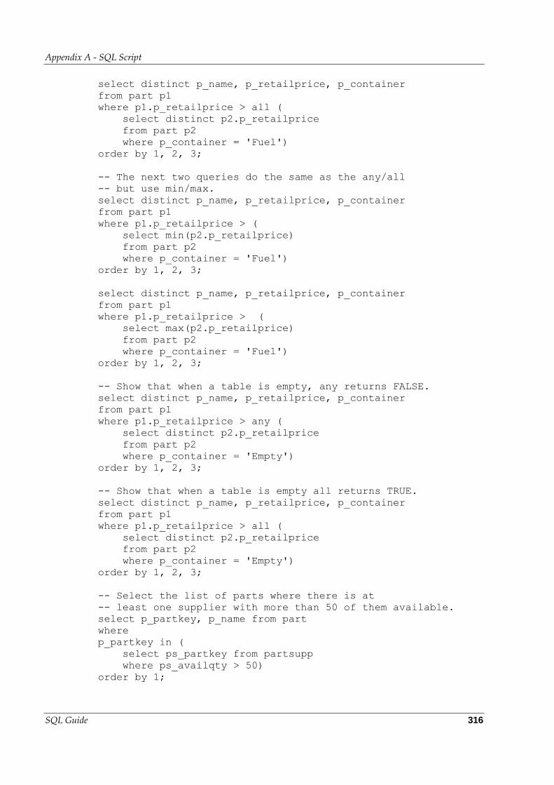
Appendix A - SQL Script
SQL Guide 316
select distinct p_name, p_retailprice, p_container
from part p1
where p1.p_retailprice > all (
select distinct p2.p_retailprice
from part p2
where p_container = 'Fuel')
order by 1, 2, 3;
-- The next two queries do the same as the any/all
-- but use min/max.
select distinct p_name, p_retailprice, p_container
from part p1
where p1.p_retailprice > (
select min(p2.p_retailprice)
from part p2
where p_container = 'Fuel')
order by 1, 2, 3;
select distinct p_name, p_retailprice, p_container
from part p1
where p1.p_retailprice > (
select max(p2.p_retailprice)
from part p2
where p_container = 'Fuel')
order by 1, 2, 3;
-- Show that when a table is empty, any returns FALSE.
select distinct p_name, p_retailprice, p_container
from part p1
where p1.p_retailprice > any (
select distinct p2.p_retailprice
from part p2
where p_container = 'Empty')
order by 1, 2, 3;
-- Show that when a table is empty all returns TRUE.
select distinct p_name, p_retailprice, p_container
from part p1
where p1.p_retailprice > all (
select distinct p2.p_retailprice
from part p2
where p_container = 'Empty')
order by 1, 2, 3;
-- Select the list of parts where there is at
-- least one supplier with more than 50 of them available.
select p_partkey, p_name from part
where
p_partkey in (
select ps_partkey from partsupp
where ps_availqty > 50)
order by 1;
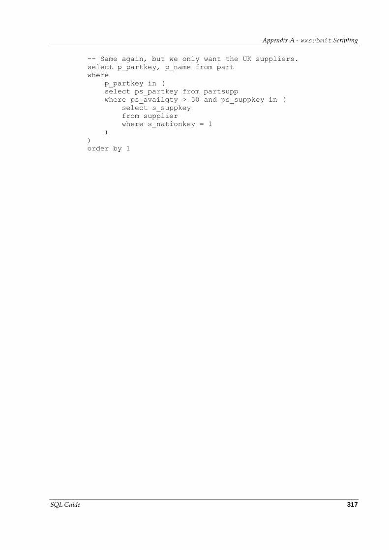
Appendix A - wxsubmit Scripting
SQL Guide 317
-- Same again, but we only want the UK suppliers.
select p_partkey, p_name from part
where
p_partkey in (
select ps_partkey from partsupp
where ps_availqty > 50 and ps_suppkey in (
select s_suppkey
from supplier
where s_nationkey = 1
)
)
order by 1
SQL Guide 318
B
wxsubmit Scripting
wxsubmit is a command line tool to run SQL on Kognitio and display any results. The tool has extensive help that can be accessed by using the –help option. This appendix provides a brief description of using wxsubmit to develop SQL scripts; in particular it focuses on control flow and variables; a simple example of a script used to control a RECLAIM process is also included.
B.1 Variables
Variables are set using:
set var variable-name variable-value
Variables are referenced by preceding the variable name with a dollar sign.
There is also an alternative syntax which can be used to set variables:
setvar variable-name=variable-value
variable-name=variable-value
With the later syntax, any enclosing quotes are not considered part of the value. Any part of variable-value in quotes needs any contained quotes of the same type to be escaped by repetition.
Variable names may contain letters, numbers and underscores, and must begin with a letter or an underscore.
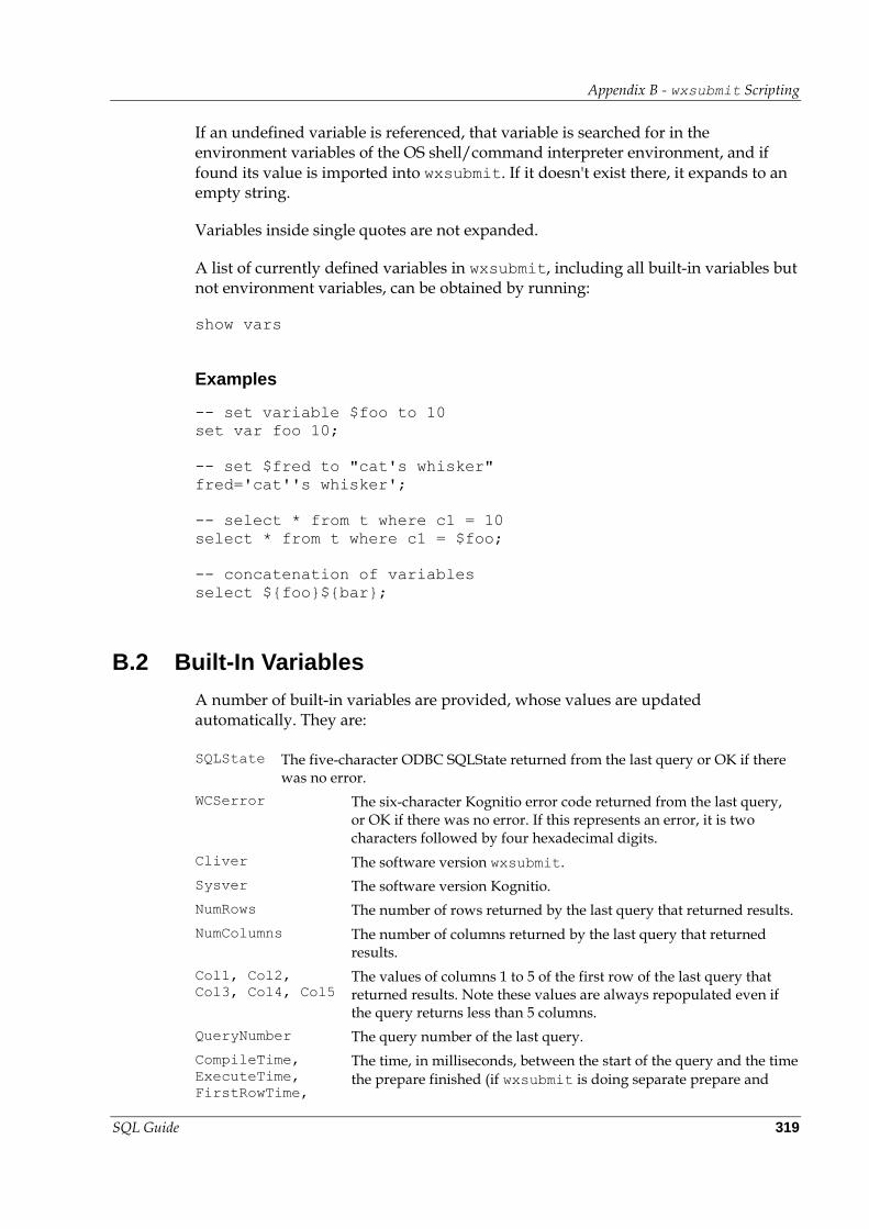
Appendix B - wxsubmit Scripting
SQL Guide 319
If an undefined variable is referenced, that variable is searched for in the environment variables of the OS shell/command interpreter environment, and if found its value is imported into wxsubmit. If it doesn't exist there, it expands to an empty string.
Variables inside single quotes are not expanded.
A list of currently defined variables in wxsubmit, including all built-in variables but not environment variables, can be obtained by running:
show vars
Examples
-- set variable $foo to 10
set var foo 10;
-- set $fred to "cat's whisker"
fred='cat''s whisker';
-- select * from t where c1 = 10
select * from t where c1 = $foo;
-- concatenation of variables
select ${foo}${bar};
B.2 Built-In Variables
A number of built-in variables are provided, whose values are updated automatically. They are:
SQLState The five-character ODBC SQLState returned from the last query or OK if there was no error.
WCSerror The six-character Kognitio error code returned from the last query, or OK if there was no error. If this represents an error, it is two characters followed by four hexadecimal digits.
Cliver The software version wxsubmit.
Sysver The software version Kognitio.
NumRows The number of rows returned by the last query that returned results.
NumColumns The number of columns returned by the last query that returned results.
Col1, Col2,
Col3, Col4, Col5
The values of columns 1 to 5 of the first row of the last query that returned results. Note these values are always repopulated even if the query returns less than 5 columns.
QueryNumber The query number of the last query.
CompileTime,
ExecuteTime,
FirstRowTime,
The time, in milliseconds, between the start of the query and the time
the prepare finished (if wxsubmit is doing separate prepare and
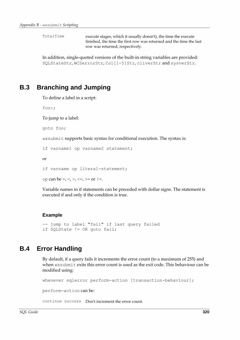
Appendix B - wxsubmit Scripting
SQL Guide 320
TotalTime execute stages, which it usually doesn't), the time the execute finished, the time the first row was returned and the time the last row was returned, respectively.
In addition, single-quoted versions of the built-in string variables are provided: SQLStateStr, WCSerrorStr, Col[1-5]Str, cliverStr and sysverStr.
B.3 Branching and Jumping
To define a label in a script:
foo:;
To jump to a label:
goto foo;
wxsubmit supports basic syntax for conditional execution. The syntax is:
if varname1 op varname2 statement;
or
if varname op literal-statement;
op can be =, <, >, <=, >= or !=.
Variable names in if statements can be preceded with dollar signs. The statement is executed if and only if the condition is true.
Example
-- jump to label "fail" if last query failed
if SQLState != OK goto fail;
B.4 Error Handling
By default, if a query fails it increments the error count (to a maximum of 255) and when wxsubmit exits this error count is used as the exit code. This behaviour can be modified using:
whenever sqlerror perform-action [transaction-behaviour];
perform-action can be:
continue success Don't increment the error count.
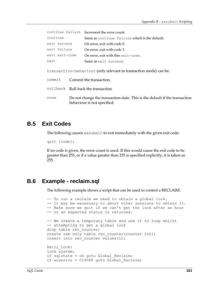
Appendix B - wxsubmit Scripting
SQL Guide 321
continue failure Increment the error count.
continue Same as continue failure which is the default.
exit success On error, exit with code 0.
exit failure On error, exit with code 1.
exit exit-code On error, exit with this exit-code.
exit Same as exit success.
transaction-behaviour (only relevant in transaction mode) can be:
commit Commit the transaction.
rollback Roll-back the transaction.
none Do not change the transaction state. This is the default if the transaction behaviour is not specified.
B.5 Exit Codes
The following causes wxsubmit to exit immediately with the given exit code:
quit [code];
If no code is given, the error count is used. If this would cause the exit code to be greater than 255, or if a value greater than 255 is specified explicitly, it is taken as 255.
B.6 Example - reclaim.sql
The following example shows a script that can be used to control a RECLAIM.
-- To run a reclaim we need to obtain a global lock.
-- It may be necessary to abort other sessions to obtain it.
-- Make sure we quit if we can't get the lock after an hour
-- or an expected status is returned.
-- We create a temporary table and use it to loop whilst
-- attempting to get a global lock
drop table rec_counter;
create ram only table rec_counter(counter int);
insert into rec_counter values(1);
Retry_Lock:
lock system;
if sqlstate = ok goto Global_Reclaim;
if wcserror = CI4088 goto Global_Reclaim;
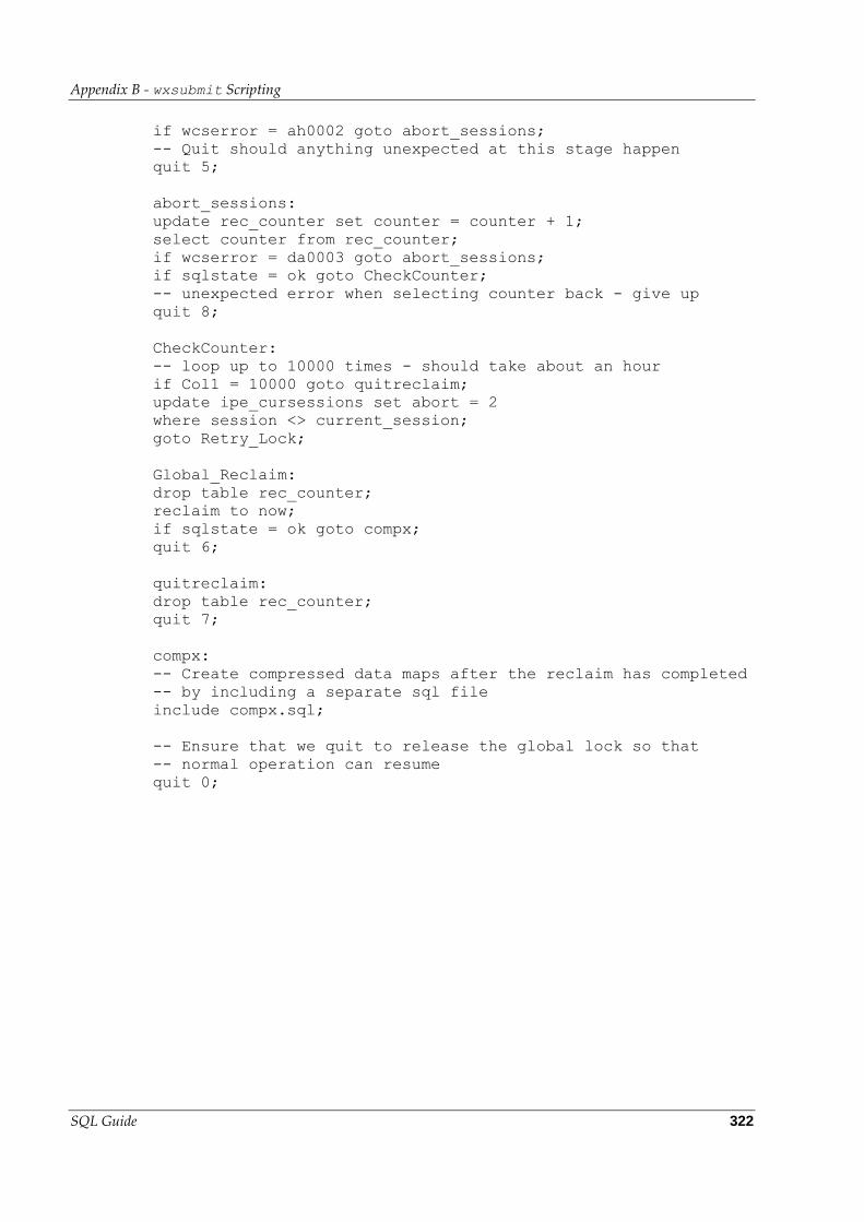
Appendix B - wxsubmit Scripting
SQL Guide 322
if wcserror = ah0002 goto abort_sessions;
-- Quit should anything unexpected at this stage happen
quit 5;
abort_sessions:
update rec_counter set counter = counter + 1;
select counter from rec_counter;
if wcserror = da0003 goto abort_sessions;
if sqlstate = ok goto CheckCounter;
-- unexpected error when selecting counter back - give up
quit 8;
CheckCounter:
-- loop up to 10000 times - should take about an hour
if Col1 = 10000 goto quitreclaim;
update ipe_cursessions set abort = 2
where session <> current_session;
goto Retry_Lock;
Global_Reclaim:
drop table rec_counter;
reclaim to now;
if sqlstate = ok goto compx;
quit 6;
quitreclaim:
drop table rec_counter;
quit 7;
compx:
-- Create compressed data maps after the reclaim has completed
-- by including a separate sql file
include compx.sql;
-- Ensure that we quit to release the global lock so that
-- normal operation can resume
quit 0;
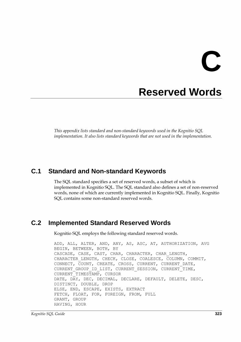
Kognitio SQL Guide 323
C
Reserved Words
This appendix lists standard and non-standard keywords used in the Kognitio SQL implementation. It also lists standard keywords that are not used in the implementation.
C.1 Standard and Non-standard Keywords
The SQL standard specifies a set of reserved words, a subset of which is implemented in Kognitio SQL. The SQL standard also defines a set of non-reserved words, none of which are currently implemented in Kognitio SQL. Finally, Kognitio SQL contains some non-standard reserved words.
C.2 Implemented Standard Reserved Words
Kognitio SQL employs the following standard reserved words.
ADD, ALL, ALTER, AND, ANY, AS, ASC, AT, AUTHORIZATION, AVG
BEGIN, BETWEEN, BOTH, BY
CASCADE, CASE, CAST, CHAR, CHARACTER, CHAR_LENGTH,
CHARACTER_LENGTH, CHECK, CLOSE, COALESCE, COLUMN, COMMIT,
CONNECT, COUNT, CREATE, CROSS, CURRENT, CURRENT_DATE,
CURRENT_GROUP_ID_LIST, CURRENT_SESSION, CURRENT_TIME,
CURRENT_TIMESTAMP, CURSOR
DATE, DAY, DEC, DECIMAL, DECLARE, DEFAULT, DELETE, DESC,
DISTINCT, DOUBLE, DROP
ELSE, END, ESCAPE, EXISTS, EXTRACT
FETCH, FLOAT, FOR, FOREIGN, FROM, FULL
GRANT, GROUP
HAVING, HOUR
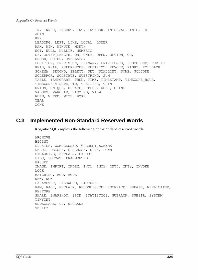
Appendix C - Reserved Words
SQL Guide 324
IN, INNER, INSERT, INT, INTEGER, INTERVAL, INTO, IS
JOIN
KEY
LEADING, LEFT, LIKE, LOCAL, LOWER
MAX, MIN, MINUTE, MONTH
NOT, NULL, NULLIF, NUMERIC
OF, OCTET_LENGTH, ON, ONLY, OPEN, OPTION, OR,
ORDER, OUTER, OVERLAPS,
POSITION, PRECISION, PRIMARY, PRIVILEGES, PROCEDURE, PUBLIC
READ, REAL, REFERENCES, RESTRICT, REVOKE, RIGHT, ROLLBACK
SCHEMA, SECOND, SELECT, SET, SMALLINT, SOME, SQLCODE,
SQLERROR, SQLSTATE, SUBSTRING, SUM
TABLE, TEMPORARY, THEN, TIME, TIMESTAMP, TIMEZONE_HOUR,
TIMEZONE_MINUTE, TO, TRAILING, TRIM
UNION, UNIQUE, UPDATE, UPPER, USER, USING
VALUES, VARCHAR, VARYING, VIEW
WHEN, WHERE, WITH, WORK
YEAR
ZONE
C.3 Implemented Non-Standard Reserved Words
Kognitio SQL employs the following non-standard reserved words.
ARCHIVE
BIGINT
CLUSTER, COMPRESSED, CURRENT_SCHEMA
DEBUG, DECODE, DIAGNOSE, DISK, DOWN
EXCLUSIVE, EXPLAIN, EXPORT
FILE, FORMAT, FRAGMENTED
HASHED
IMAGE, IMPORT, INDEX, INT1, INT2, INT4, INT8, INVOKE
LOCK
MATCHING, MOD, MODE
NEW, NOW
PARAMETER, PASSWORD, PICTURE
RAM, RACK, RECLAIM, RECONFIGURE, RECREATE, REPAIR, REPLICATED,
RESTORE
SHARE, SNAPSHOT, SPIN, STATISTICS, SUBRACK, SUBSTR, SYSTEM
TINYINT
UNDECLARE, UP, UPGRADE
VERIFY
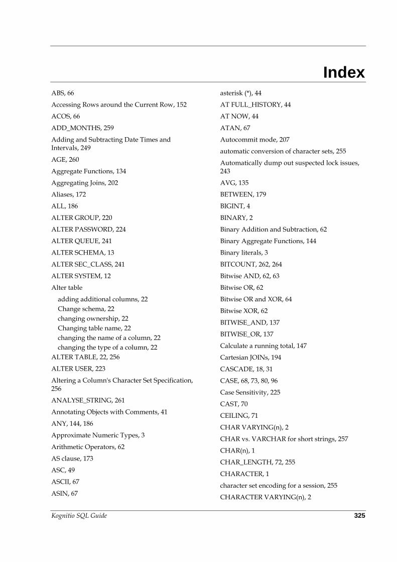
Kognitio SQL Guide 325
Index ABS, 66
Accessing Rows around the Current Row, 152
ACOS, 66
ADD_MONTHS, 259
Adding and Subtracting Date Times and Intervals, 249
AGE, 260
Aggregate Functions, 134
Aggregating Joins, 202
Aliases, 172
ALL, 186
ALTER GROUP, 220
ALTER PASSWORD, 224
ALTER QUEUE, 241
ALTER SCHEMA, 13
ALTER SEC_CLASS, 241
ALTER SYSTEM, 12
Alter table
adding additional columns, 22
Change schema, 22
changing ownership, 22
Changing table name, 22
changing the name of a column, 22
changing the type of a column, 22
ALTER TABLE, 22, 256
ALTER USER, 223
Altering a Column's Character Set Specification, 256
ANALYSE_STRING, 261
Annotating Objects with Comments, 41
ANY, 144, 186
Approximate Numeric Types, 3
Arithmetic Operators, 62
AS clause, 173
ASC, 49
ASCII, 67
ASIN, 67
asterisk (*), 44
AT FULL_HISTORY, 44
AT NOW, 44
ATAN, 67
Autocommit mode, 207
automatic conversion of character sets, 255
Automatically dump out suspected lock issues, 243
AVG, 135
BETWEEN, 179
BIGINT, 4
BINARY, 2
Binary Addition and Subtraction, 62
Binary Aggregate Functions, 144
Binary literals, 3
BITCOUNT, 262, 264
Bitwise AND, 62, 63
Bitwise OR, 62
Bitwise OR and XOR, 64
Bitwise XOR, 62
BITWISE_AND, 137
BITWISE_OR, 137
Calculate a running total, 147
Cartesian JOINs, 194
CASCADE, 18, 31
CASE, 68, 73, 80, 96
Case Sensitivity, 225
CAST, 70
CEILING, 71
CHAR VARYING(n), 2
CHAR vs. VARCHAR for short strings, 257
CHAR(n), 1
CHAR_LENGTH, 72, 255
CHARACTER, 1
character set encoding for a session, 255
CHARACTER VARYING(n), 2
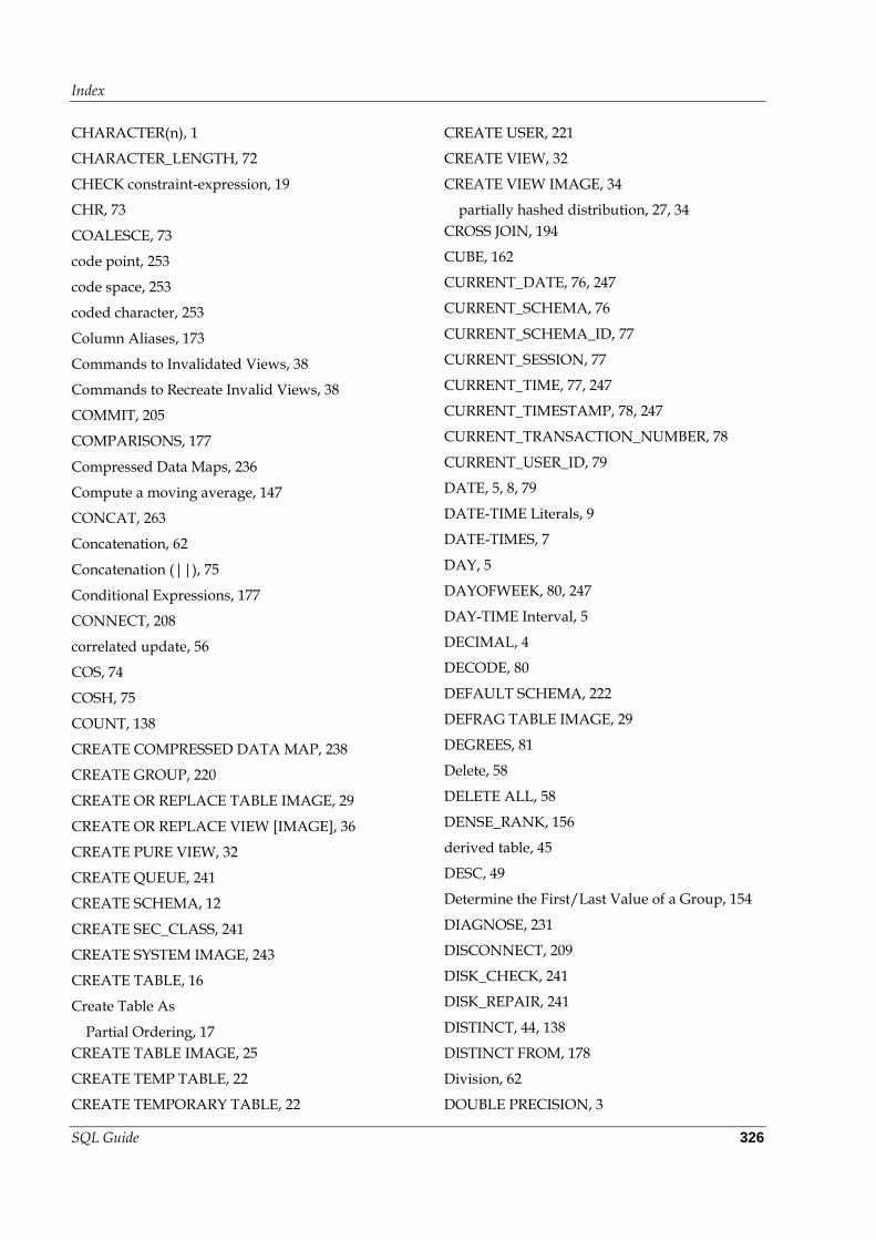
Index
SQL Guide 326
CHARACTER(n), 1
CHARACTER_LENGTH, 72
CHECK constraint-expression, 19
CHR, 73
COALESCE, 73
code point, 253
code space, 253
coded character, 253
Column Aliases, 173
Commands to Invalidated Views, 38
Commands to Recreate Invalid Views, 38
COMMIT, 205
COMPARISONS, 177
Compressed Data Maps, 236
Compute a moving average, 147
CONCAT, 263
Concatenation, 62
Concatenation (||), 75
Conditional Expressions, 177
CONNECT, 208
correlated update, 56
COS, 74
COSH, 75
COUNT, 138
CREATE COMPRESSED DATA MAP, 238
CREATE GROUP, 220
CREATE OR REPLACE TABLE IMAGE, 29
CREATE OR REPLACE VIEW [IMAGE], 36
CREATE PURE VIEW, 32
CREATE QUEUE, 241
CREATE SCHEMA, 12
CREATE SEC_CLASS, 241
CREATE SYSTEM IMAGE, 243
CREATE TABLE, 16
Create Table As
Partial Ordering, 17
CREATE TABLE IMAGE, 25
CREATE TEMP TABLE, 22
CREATE TEMPORARY TABLE, 22
CREATE USER, 221
CREATE VIEW, 32
CREATE VIEW IMAGE, 34
partially hashed distribution, 27, 34
CROSS JOIN, 194
CUBE, 162
CURRENT_DATE, 76, 247
CURRENT_SCHEMA, 76
CURRENT_SCHEMA_ID, 77
CURRENT_SESSION, 77
CURRENT_TIME, 77, 247
CURRENT_TIMESTAMP, 78, 247
CURRENT_TRANSACTION_NUMBER, 78
CURRENT_USER_ID, 79
DATE, 5, 8, 79
DATE-TIME Literals, 9
DATE-TIMES, 7
DAY, 5
DAYOFWEEK, 80, 247
DAY-TIME Interval, 5
DECIMAL, 4
DECODE, 80
DEFAULT SCHEMA, 222
DEFRAG TABLE IMAGE, 29
DEGREES, 81
Delete, 58
DELETE ALL, 58
DENSE_RANK, 156
derived table, 45
DESC, 49
Determine the First/Last Value of a Group, 154
DIAGNOSE, 231
DISCONNECT, 209
DISK_CHECK, 241
DISK_REPAIR, 241
DISTINCT, 44, 138
DISTINCT FROM, 178
Division, 62
DOUBLE PRECISION, 3
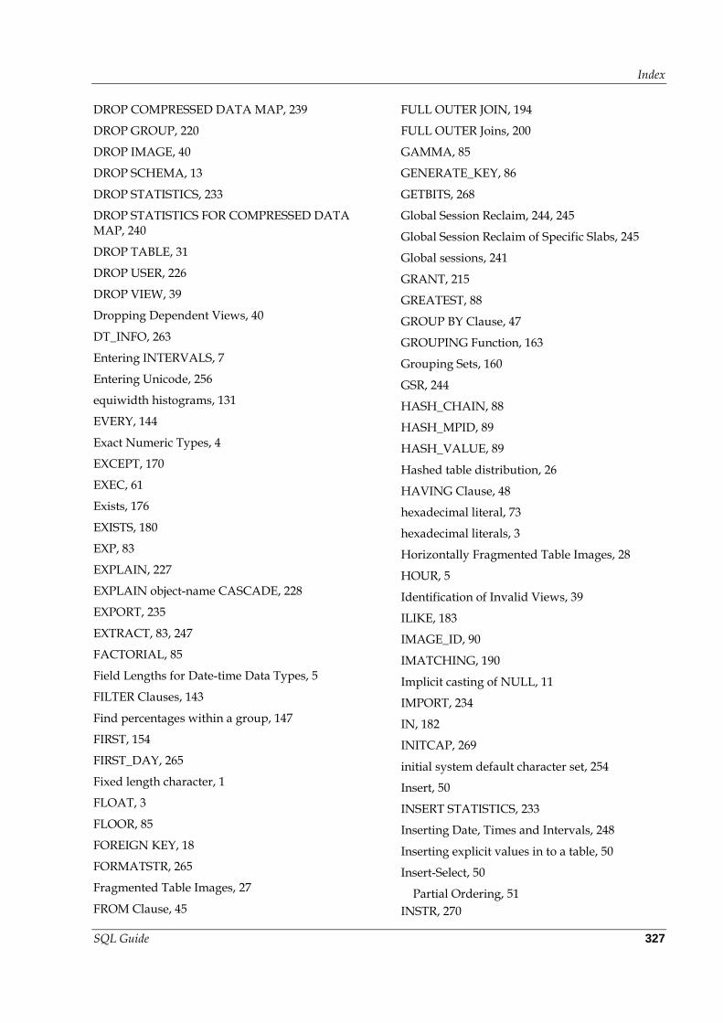
Index
SQL Guide 327
DROP COMPRESSED DATA MAP, 239
DROP GROUP, 220
DROP IMAGE, 40
DROP SCHEMA, 13
DROP STATISTICS, 233
DROP STATISTICS FOR COMPRESSED DATA MAP, 240
DROP TABLE, 31
DROP USER, 226
DROP VIEW, 39
Dropping Dependent Views, 40
DT_INFO, 263
Entering INTERVALS, 7
Entering Unicode, 256
equiwidth histograms, 131
EVERY, 144
Exact Numeric Types, 4
EXCEPT, 170
EXEC, 61
Exists, 176
EXISTS, 180
EXP, 83
EXPLAIN, 227
EXPLAIN object-name CASCADE, 228
EXPORT, 235
EXTRACT, 83, 247
FACTORIAL, 85
Field Lengths for Date-time Data Types, 5
FILTER Clauses, 143
Find percentages within a group, 147
FIRST, 154
FIRST_DAY, 265
Fixed length character, 1
FLOAT, 3
FLOOR, 85
FOREIGN KEY, 18
FORMATSTR, 265
Fragmented Table Images, 27
FROM Clause, 45
FULL OUTER JOIN, 194
FULL OUTER Joins, 200
GAMMA, 85
GENERATE_KEY, 86
GETBITS, 268
Global Session Reclaim, 244, 245
Global Session Reclaim of Specific Slabs, 245
Global sessions, 241
GRANT, 215
GREATEST, 88
GROUP BY Clause, 47
GROUPING Function, 163
Grouping Sets, 160
GSR, 244
HASH_CHAIN, 88
HASH_MPID, 89
HASH_VALUE, 89
Hashed table distribution, 26
HAVING Clause, 48
hexadecimal literal, 73
hexadecimal literals, 3
Horizontally Fragmented Table Images, 28
HOUR, 5
Identification of Invalid Views, 39
ILIKE, 183
IMAGE_ID, 90
IMATCHING, 190
Implicit casting of NULL, 11
IMPORT, 234
IN, 182
INITCAP, 269
initial system default character set, 254
Insert, 50
INSERT STATISTICS, 233
Inserting Date, Times and Intervals, 248
Inserting explicit values in to a table, 50
Insert-Select, 50
Partial Ordering, 51
INSTR, 270
Index
SQL Guide 328
INT, 4
INT1, 4
INT2, 4
INT4, 4
INT8, 4
INTEGER, 4
INTERSECT, 171
INTERVAL, 5
Intervals, Dates and Times, 5
INTTOSTR, 91
Invalidated Views, 38
IPE_CHARACTER_SET, 254
IPE_CHARSET_TRANSLATION, 254
IPE_FIELD, 234
IPE_FILE, 234
IPE_FILE_FORMAT, 234
IPE_REM_SERVER, 234
IPE_REM_USER, 234
IS NULL, 189
IS_DATE, 271
Join Operators, 193
Kognitio Administrative Functions, 241
Labeling the Result Column for CASE, 174
Labelling Simple Expressions, 173
LAG, 153
LAST, 154
LAST_DAY, 273
Latin-1, 253
LEAD, 153
LEAST, 92
LEFT, 92
LEFT OUTER JOIN, 194
LEFT OUTER Joins, 197
LENGTH, 72
LIKE, 183
LN, 94
LOCK SYSTEM, 241
LOCK TABLE, 242
LOG10, 93
LOWER, 93
LPAD, 94
LTRIM, 274
MAPDAY, 274
MAPMONTH, 275
MATCHING, 190
MAX, 140
Maximum String Length, 3
Maximum/minimum values supported for integers, 4
Maximum/minimum values supported for REAL and FLOAT, 3
MAXLIST, 88, 95
MERGE, 59
MIN, 141
MINLIST, 92, 95
MINUS, 170
MINUTE, 5
MOD, 65, 96
Modulus, 62
MONTH, 5
MONTHS_BETWEEN, 275
Multiplication, 62
NATURAL JOIN, 194
natural logarithm, 94
NCHAR, 2
Nested sub-SELECTs, 176
New System, 241
NEXT_DAY, 276
NFS Import and Export, 234
NOT NULL, 18
NTILE, 158
NULL, 18
NULLIF, 96
NULLs, 10
NUMERIC, 4
NVARCHAR, 2
NVL, 97
Index
SQL Guide 329
OCTET_LENGTH, 72, 97, 255
OLAP Basics, 159
OLAP Examples, 163
OLAP Functions, 159
Omitting FROM clause, 45
Operations that cannot be rolled back, 207
ORDER BY Clause, 49
outer join
the (+) syntax, 195
OVERLAPS, 188
OVERLAY, 97
Overview, 253
Overview of Analytic Functions, 147
PACKDATE, 98, 247
pad character, 2
Partial distributions, 26
PARTITION BY clause, 149
PASSWORD, 222
PI, 98
PICTURE, 229
POSITION, 98
POSN_IN_LIST, 100
POWER, 101
precision, 4
PRIMARY, 18
PROFILE, 277
RADIANS, 101
RAM image of a table, 25, 29
RAM Only Temporary Table, 18
RAM ONLY TEMPORARY TABLE (ROTTs), 30
Random table distribution, 26
Range Windows, 151
RANK, 156
Ranking and Windowing Analytic Functions, 147
RATIO_TO_REPORT, 159
REAL, 3
RECLAIM, 31, 244
RECLAIM TO NOW, 245
RECREATE, 241
Regular expression matching, 190
RENAME TABLE, 25
REPLACE, 278
Replicated table distribution, 26
RESTRICT, 18, 31
REVERSE, 278
REVOKE, 217, 224
RIGHT, 102
RIGHT OUTER JOIN, 194
RIGHT OUTER Joins, 199
ROLLBACK, 205, 206
ROLLUP, 161
ROUND, 279
ROUND
format models, 280
ROUND (date), 280
ROUND (time), 280
ROUND (timestamp), 280
ROUND(number), 280
row value constructors, 175
Row Windows, 150
ROW_NUMBER, 154
RPAD, 102
RTRIM, 281
Running Totals, 152
RVC, 175
Scalar Operators and Functions, 62
scale, 4
SCHEMA, 222
schema default character set, 254
SCHEMA_ID, 103
Search Condition, 46
Searched Case Expression, 68
SEC_CLASS, 222
SECOND, 5
SELECT Clause, 44
SELECT statement, 43
Self-Join, 47
Index
SQL Guide 330
SET DEFAULT, 18
SET DEFAULT SCHEMA, 224
SET MODE, 207
SET NULL, 18
Set Operations, 168
EXCEPT, 168
INTERSECT, 168
UNION, 168
SET SCHEMA, 15
SET SEC_CLASS, 224
SET TIME ZONE, 10
SIGN, 104
SIMILAR TO, 185
Simple Case Expression, 68
SIN, 105
SINH, 105
SINKCHARS, 282
Skewed data, 26
SMALLINT, 4
SNIPCHARS, 283
SOME, 144, 186
Sorting in Descending Order, 50
SOUNDEX, 106
SPIN, 241
SQRT, 106
Square root, 106
Standard Deviation, 142
Statistics, 231
STDEV, 142
STRCHOP, 107
STRCOUNT, 109
String comparison and sorting, 255
String Data Types, 1
STRPACKINTS, 110
STRPOS, 111
STRTOINT, 112
STRUNPACKINTS, 114
sub-SELECT, 174
Sub-SELECTS in WHERE and CASE clauses, 175
SUBSTR, 284
SUBSTRING, 115
SUCKCHARS, 285
SUM, 142
SWAPCHARS, 286
Syntax of Ranking and Windowing functions, 149
SYSDATE, 117
system default character set, 254
Table Aliases, 172
TABLE_ID, 117
TABLESAMPLE, 45
TAN, 117
TANH, 118
Temporary RAM-only tables, 21
Temporary Tables, 21
TIME, 5, 8, 118
TIME WITH TIME ZONE, 9
TIME ZONES, 9
TIMESTAMP, 5, 8, 119
TIMESTAMP WITH TIMEZONE, 9
TINYINT, 4
TO_CHAR, 120, 287
TO_DATE, 124, 292
TO_NUMBER, 293
TO_TIME, 125, 294
TO_TIMESTAMP, 126, 295
Top-N queries, 147
Transaction Control, 205
Transaction mode, 207
TRANSLATE, 296
TRIM, 126
TRUNC, 296
TRUNC
format models, 280
TRUNC (date), 297
TRUNC (number), 297
TRUNC (time), 297
TRUNC (timestamp), 297
Index
SQL Guide 331
Truncate Table, 58
UCHR, 128
UCS-2, 254
Unary negative and positive, 62
Unicode, 253
UNICODE, 128
Unicode Standard, 253
UNION, 169
UNIQUE, 181
UNIQUE, 18
Update, 55
UPDATE STATISTICS, 231
UPDATE STATISTICS FOR COMPRESSED DATA MAP, 236
UPPER, 129
USER, 129
USER_ID, 130
Users and Groups, 219
Using Date-time Data Types, 8
Using Date-times and Intervals, 247
Using literal values instead of a table or view, 45
Using National Character Sets, 253
using parentheses to enclose join expressions, 193
Using Table Name Aliases, 46
UTF-16, 254
UTF-32, 254
UTF-8, 254
VAL_AT_POSN, 130
VAR, 143
VARBINARY, 2
VARCHAR, 2
VARCHAR(n), 2
VARCHAR2(n), 2
Variable length character, 2
Variance, 143
WCB format, 234
WHERE clause
the (+) syntax, 195
WHERE Clause, 46
WIDTH_BUCKET, 131
Windowing-Clause, 149
WITH CHECK OPTION, 32, 51
WITH Clause, 44
WITH GRANT OPTION, 215
WX_CREATE_TNO, 132
WX_UPDATE_TNO, 133
Kognitio Character Set Specification, 254
WXDataport utility, 235
YEAR, 5
YEAR-MONTH Interval, 5
![Microsoft SQLEKM Provider€¦ · CREATE DATABASE utimaco GO USE utimaco CREATE TABLE [dbo].[demo] (firstname varchar (255) NOT NULL, name varchar (255) NOT NULL, secret varbinary](https://img.pdfslide.us/doc/110x75/5fd6953e7fa4c053d43cad76/microsoft-sqlekm-provider-create-database-utimaco-go-use-utimaco-create-table-dbodemo.jpg)