Knt . Alfn, å - ssb.no · Abtrt Knt . Alfn, l nd Klrd Enr dnd rbn n nd d rn Cnn f hnn Wtrn Erp prt 9/1 • Sttt r 199 Epln lttr nr dnd dl f thrtn Wtrn Erpn ntr (SEEM tthr th th

96/12 Rapporter Reports

Knut H. Alfsen, På l Boug andDag Kolsrud

Energy demand, carbonemissions and acid rainConsequences of a changing WesternEurope

Statistisk sentralbyrå • Statistics NorwayOslo—Kongsvinger 1996

Standardtegn i tabellerTall kan ikke forekommeOppgave manglerOppgave mangler forelopigTall kan ikke offentliggjoresNullMindre enn 0,5av den brukte enhetenMindre enn 0,05av den brukte enhetenForelopige tallBrudd i den loddrette serien

Symbols in tables Category not applicableData not availableData not yet availableNot for publication NilLess than 0.5 of unitemployedLess than 0.05 of unitemployedProvisional or preliminary figureBreak in the homogeneity of a vertical series

Symbol

••

•••

-

0

0,0*

Brudd i den vannrette serien Break in the homogeneity of a horizontal series IRettet siden forrige utgave Revised since the previous issue r

ISBN 82-537-4285-1ISSN 0806-2056

Emnegruppe01 Naturressurser og naturmiljo

EmneordEnergiettersporselLuftforurensningØkonomisk vekstScenarierSEEMSur nedborVest-Europa

Design: Enzo Finger DesignTrykk: Statistisk sentralbyr6

Abstract

Knut H. Alfsen, Pal Boug and Dag Kolsrud

Energy demand, carbon emissions and acid rainConsequences of a changing Western Europe

Reports 96/12 • Statistics Norway 1996

Employing a multisector energy demand model of thirteen Western European countries (SEEM) together with theRAINS model developed by IIASA, we in this report address the question of how much the European economic andpolitical integration process matter for future development in energy demand, emissions to air of key pollutants andtransboundary transport of sulphur and nitrogen. We do this by comparing two simulation scenarios; one scenariobased on the assumption of further European integration versus another scenario where fragmentation is assumed toprevail. Both scenarios cover the period from 1991 to 2020. The focus of the report is on consequences for futuredemand for fossil fuels, emissions of CO2, SO2 and NO., and transport and deposition of sulphur and nitrogen.

Average annual growth in GDP in the integration scenario is 2.3 per cent, while demand for energy, emissions of CO2,SO2 and NO., and nitrogen deposition all show average annual growth rates from 1.7 to 1.9 per cent. Deposition ofsulphur grows at the slightly lower rate of 1.4 per cent per year in this scenario. In the fragmentation scenario allgrowth rates are reduced by 0.5-0.7 percentage points, except the rate of annual average growth in SO2 emissionswhich is reduced by 0.8 percentage point. The results vary considerably, however, over countries, sectors and fueltypes.

Keywords: Energy demand, emissions to air, economic growth, SEEM, acid rain, Western-Europe.

Acknowledgement: This paper is an outcome of the project "Energy scenarios for a changing Europe" carried outat Statistics Norway in cooperation with ECN, The Netherlands. Financial support from Statoil, The Dutch Ministry ofPlanning and The Norwegian Ministry of Environment is acknowledged.

3

Reports 96/12 Energy demand and emissions

Contents1. Introduction 7

2. The SEEM model 82.1. Model structure 82.2. The sector models 92.3. Model input and output 10

3. Integration or fragmentation? A brief description of alternative economic scenarios 123.1. Ongoing Western European Integration (IS) 123.2. Western European Fragmentation (FS) 133.3. Model inputs 133.3.1. Economic growth 133.3.2. Energy prices 143.3.3. Autonomous efficiency improvement 14

4. Simulation results 154.1. Energy demand 154.2. Emissions to air 184.2.1. Emission of CO2 184.2.2. Emission of SO2 and NO 194.2.3. Deposition of SO 2 and NO 20

5. Conclusion 22

References 23

Appendix: Country tables 24

Previously issued on the subject 25

Recent publications in the series Reports 26

5


1. Introduction

European integration has been on the agenda for along time. Whether this momentum towards greaterintegration can be kept up also in the next few decadesis however uncertain. The problem addressed in thisreport is how this uncertainty might affect its energymarkets and how this in turn could affect emissions ofcarbon dioxide (CO2), and emissions, transport anddeposition of the two most important acid compounds;sulphur dioxide (SO2) and nitrogen oxides (NO.).

The strategy followed is first to describe how furtherintegration or lack of integration (fragmentation) canaffect the economic development of 13 countries inWestern Europe. This description is of an ad hoc natureand is treated as exogenous input to this analysis.Based on alternative growth paths, we employ aSectoral European Energy Model (SEEM) to calculatelikely impacts on the energy markets, where basicallythree types of primary energy goods are treatedendogeneously; gaseous fuels, liquid fuels and solidfuels1. Supply and demand of electricity based onthermal power production is also modelled in SEEM.

Other types of energy technologies, e.g. nuclear powerand alternative energy technologies, are treated asexogenously given. Secondly, based on projectedenergy demand, emissions of the greenhouse gascarbon dioxide (CO2) is calculated by the SEEMmodel', while IIASA's RAINS model is utilised incalculating emissions, atmospheric transport anddeposition of SO2 and NOR. The inputs to the RAINSmodel are the energy consumption paths generated bythe SEEM model.

Given this strategy, the rest of the report is organisedas follows. The next section briefly describes thestructure and working of the SEEM model'. Section 3then comments on the economic assumptions used inthe two scenarios of further European integration and

1 Studies based on a previous version of the model have beenpublished by Birkelund et al. (1993, 1994) and Alfsen et al. (1995).2 The topic of CO2 emissions in a changing Europe is discussed indetail in Boug and Brubakk (1996).3 The model is documented in detail in Brubakk et al. (1995), Boug(1995) and Kolsrud (1996).

European fragmentation, respectively. Simulationresults based on these alternative economic develop-ment paths are given in section 4, while section 5concludes. The appendix contains a set of detailedcountry tables covering emissions to air and depositionof SO2 and NOR.

7

Energy demand and emissions Reports 96/12

2. The SEEM model

2.1. Model structureThe Sectoral European Energy Model (SEEM)4 is asimulation model for energy demand projections for 13countries in Western Europe. The model consists ofseparate model blocks for each of the followingcountries:• Four major energy consumers: Germany, France,

United Kingdom, and Italy;• Four Nordic countries: Denmark, Sweden, Finland

and Norway;• Five other countries: Spain, the Netherlands,

Belgium, Austria, and Switzerland.

Together, these countries consumed about 90 per centof the total energy use in the OECD Europe in 1991.

Neither inter-country trade nor supply of primaryenergy is modelled within SEEM. Supply of electricpower is, however, part of the model. In each countrythere are five sectors: manufacturing industries andservice industries (hereafter referred to as industry andservices), households, transport' and power produc-tion. Energy commodities covered in SEEM are coal,oil, gas, electricity and various transport fuels. De-mands for nuclear and renewable fuels are treated asgiven in the model.

The model is partial in the sense that it determines thedemand for energy based on exogenous prices, taxesand production and consumption activity levels (cf. fig-ure 2.1). Hence, we focus on the demand side of theenergy markets, with the assumption that demandequals realised consumption. However, both the de-mand and the supply side of the Electricity generatingsector is included in the model. Cost minimisingbehaviour is assumed for all sectors using energy.

The choice of behavioural functional forms and para-meters, and the quantitative methodology, were chosenconsidering the data and resource limitations.

4 SEEM version 2.0 has been developed in co-operation with theNetherlands Energy Research Foundation ECN.5 Fuel demand for transport purposes has been grouped into onesector.

Furthermore, model transparency and the scope forimplementation and simulation on a Personal Com-puter were important design criteria.

Parameters representing the behaviour of the sectorsincluded in the model are estimated on empirical dataor calibrated on research results published in interna-tional journals. For all estimations and the calibrationof the energy use and prices to the base year (1991),data from the International Energy Agency (IEA,1993a, b) were used.

We have formulated the model equations directly atthe sector level by adopting a "top down" modellingapproach. However, the macro-level producer or con-sumer that we study, is assumed to behave accordingto microeconomic considerations. In fact, the neo-classical micro model often seems more meaningful. atthe sector level than at the individual level. In parti-cular, continuous substitution possibilities are perhapsmore realistic at a sectoral level. These substitutionpossibilities are premises for cost minimising and utilitymaximising behaviour, which are crucial assumptionswhen deriving the fuel demand functions.

Figure 2.1 depicts the structure of the model block forone country. In a first step the model determines thedemand for coal, oil, natural gas and electricity in theend user sectors, based on exogenous information onactivity levels, income, and technology, in addition toproduction factor prices.

In the electricity generation sector the need for dome-stic production of power is derived, given an exo-genous matrix of net power import and a constantpercentage of distribution losses. The electricityrequirements can be produced in several ways: Bythermal power plants using coal, oil or natural gas asinputs, by nuclear power plants and/or by plants usingrenewables (now mainly hydro power).

8

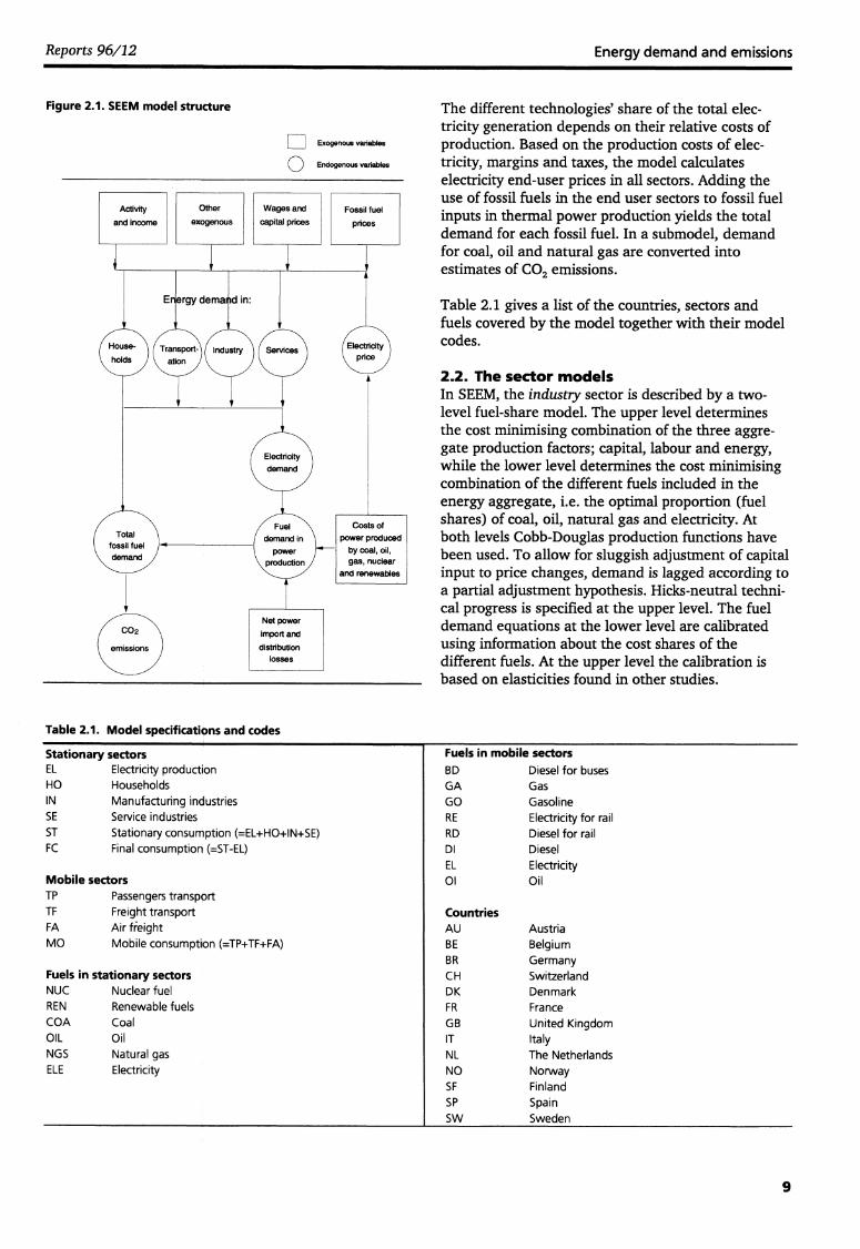
Figure 2.1. SEEM model structure

Exogenous variables

0 Endogenous variables

Activityand income

Fueldemand in

powerproduction

Net powerimport anddistribution

losses

Costs ofpower produced

by coal, oil,gas, nuclear

and renewables

Fuels in mobile sectors

BD Diesel for busesGA GasGO GasolineRE Electricity for railRD Diesel for railDI DieselEL Electricity01 Oil

CountriesAUBEBRCHDKFRGBITNLNOSFSPSW

AustriaBelgiumGermanySwitzerlandDenmarkFranceUnited KingdomItalyThe NetherlandsNorwayFinlandSpainSweden

Reports 96/12

Energy demand and emissions

The different technologies' share of the total elec-tricity generation depends on their relative costs ofproduction. Based on the production costs of elec-tricity, margins and taxes, the model calculateselectricity end-user prices in all sectors. Adding theuse of fossil fuels in the end user sectors to fossil fuelinputs in thermal power production yields the totaldemand for each fossil fuel. In a submodel, demandfor coal, oil and natural gas are converted intoestimates of CO, emissions.

Table 2.1 gives a list of the countries, sectors andfuels covered by the model together with their modelcodes.

2.2. The sector modelsIn SEEM, the industry sector is described by a two-level fuel-share model. The upper level determinesthe cost minimising combination of the three aggre-gate production factors; capital, labour and energy,while the lower level determines the cost minimisingcombination of the different fuels included in theenergy aggregate, i.e. the optimal proportion (fuelshares) of coal, oil, natural gas and electricity. Atboth levels Cobb-Douglas production functions havebeen used. To allow for sluggish adjustment of capitalinput to price changes, demand is lagged according toa partial adjustment hypothesis. Hicks-neutral techni-cal progress is specified at the upper level. The fueldemand equations at the lower level are calibratedusing information about the cost shares of thedifferent fuels. At the upper level the calibration isbased on elasticities found in other studies.

Table 2.1. Model specifications and codes

Stationary sectorsEL Electricity productionHO HouseholdsIN Manufacturing industriesSE Service industriesST Stationary consumption (=EL+H0+IN+SE)FC Final consumption (=ST-EL)

Mobile sectorsTP Passengers transportTF Freight transportFA Air fieightMO Mobile consumption (=TP+TF+FA)

Fuels in stationary sectorsNUC Nuclear fuelREN Renewable fuelsCOA CoalOIL OilNGS Natural gasELE Electricity

9


For service industries we have estimated a fuel-sharemodel similar to that of the industry sector by postu-lating Constant Elasticity of Substitution (CES)production functions for the energy aggregates. Weallow for a nested model in three levels (compared totwo in the industry sector) for countries with substan-tial use of all four energy sources, i.e coal, oil, gas andelectricity. At the upper level, electricity and an aggre-gate of oil, gas and coal are separate inputs. This im-plies a hypothesis that the use of electricity contributesto production in a profoundly different way comparedto fossil fuels. While the latter are used for space heat-ing mainly, electricity is mostly used in appliances likecomputers and lighting for which energy substitution isimpossible. The energy demand functions at the upperlevel are log-linear, with calibrated parameters. At theintermediate level, the fossil fuel aggregate is producedby a CES technology utilising an aggregate of oil andgas, and of solids. At the lower level the oil and gasaggregate is produced, also by a CES technology. Theintermediate and lower level parameters are estimated.

The household sector model is equal to the servicessector model, except that at the upper level «privateconsumption» and «prices of other goods» substitutefor the production activity level and factor costs othersthan energy costs as explanatory variables, respective-ly. Also in the households, electricity and fossil fuelprices are variables which determine the households'demand for electricity and fossil fuel aggregate at theupper level. The modelling and parametrisation of thelower levels are similar to the service sector model.

The transport sector model is divided into passengertransport, freight transport, and air transport. Fuelefficiencies in the transport sectors are based on linearpenetration of new technologies.

Air transport is treated separately because most airtransport is combined passenger and freight transport.Demand for fuel (kerosene) is modelled as a functionof the price of kerosene and gross domestic production.

For passenger transport both private and public tran-sport are considered; more specifically cars (gasoline,gasoil and gas), trains (electricity and gasoil) andbusses (diesel) are distinguished. At the upper level ofthe passenger transport model total demand for personkilometres is a function of consumer expenditures anda transport price index. At the lower level the demandfor transport is split into the different modes inproportions depending on fuel prices and capital pricesof the respective modes. This determines demand forperson kilometres by transport mode. Given figures forcar occupancy and efficiency, the corresponding fueluse is then computed.

The freight transport is modelled at the upper level byassuming that the development of domestic productiondetermines total demand for tonnes kilometres. Given

exogenous assumptions on mode shares and fuelefficiency, the demand for the different fuels are thencalculated.

In the electricity generation model the domestic powerproduction requirements are determined by adding enduser electricity demand (i.e. total demand fromindustry, services, households and transportation), netimport (exogenous) and distribution losses. Electricitycan be produced by different technologies relying ondifferent energy sources - coal, oil, natural gas, nuclearand renewables. The shares of electricity produced bydifferent fossil fuels are determined by the relativecosts of the different plants, which are a combinationof fuel costs and technology related costs. This in turndetermines demand for the different fuels, given fuelefficiency in different plants. As in the transport model,the fuel efficiency is based on the assumption of alinear penetration of new technologies.

The fuel price module computes sectoral end user pricesfor the different fuels. The end user prices are dividedinto import prices, gross margins and taxes. Forelectricity, the «import price» corresponds to theelectricity generation price calculated by the averageunit costs of producing electricity domestically. Grossmargins for all fuels include costs and profits intransformation, distribution, retailing, etc. Taxes aredivided into fuel specific taxes, carbon taxes and avalue added tax.

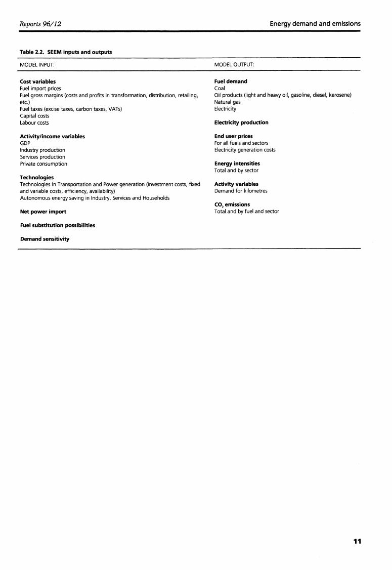
2.3. Model input and outputTable 2.2 summarises the main SEEM model input andoutput. The list reflects the menu for topics and policyquestions that the model user can study by simulatingSEEM.

10


Table 2.2. SEEM inputs and outputs

MODEL INPUT: MODEL OUTPUT:

Cost variables Fuel demandFuel import prices CoalFuel gross margins (costs and profits in transformation, distribution, retailing, Oil products (light and heavy oil, gasoline, diesel, kerosene)etc.) Natural gasFuel taxes (excise taxes, carbon taxes, VATs) ElectricityCapital costsLabour costs Electricity production

Activity/income variables End user pricesGDP For all fuels and sectorsIndustry production Electricity generation costsServices productionPrivate consumption Energy intensities

Total and by sectorTechnologiesTechnologies in Transportation and Power generation (investment costs, fixedand variable costs, efficiency, availability)Autonomous energy saving in Industry, Services and Households

Net power import

Fuel substitution possibilities

Demand sensitivity

Activity variablesDemand for kilometres

CO, emissionsTotal and by fuel and sector

11


3. Integration or fragmentation? A briefdescription of alternative economicscenarios

In this section we describe the economic developmentscenarios used as input to the SEEM model simulations,starting with the integration scenario.

3.1. Ongoing Western European Integration(IS)

This scenario is based on the assumption that theongoing European integration process will continuemore or less according to the time schedule in theMaastricht treaty. Because of perceived positive econo-mic perspectives we assume that the EU will be joinedby Switzerland and Norway around the turn of thecentury. Hence, the integration process concerns all 13Western European countries. Furthermore, we assumean association of all Central and Eastern Europeancountries around year 2000, improving trade possi-bilities and access to foreign investments. In fact weassume that all proposals mentioned in the MaastrichtTreaty are fully implemented by the year 2000. Theintegration process will result in the completion of theall objectives of the internal market, so free movementof all goods, persons and capital will be realised.

We expect that the completion of the internal marketwill have a moderate, but positive, overall effect oneconomic productivity and income in EU. Funds forstructural improvements in the Southern European EUcountries presumably will contribute to a more equaldevelopment pattern.

We expect that the European Monetary Union willresult in a single currency (ECU) and the establishmentof a Central bank before the year 2000. A stablemonetary situation without continuously changingexchange rates will be reached at that time, increasingeconomic prospects further.

Already political decisions in the field of environmentalprotection, public health and consumers' protection aremade on Communal level. With respect to envi-ronmental policy, we assume more attention will begiven to «continental» issues, e.g. Eastern Europeanproblems. Economic and social cohesion, high-techindustry and research are subjects given high priorityby the Community. EU will co-ordinate these policiesEurope-wide with a minimum of national interferenceand obstacles.

Of crucial importance to the issue analysed in thisreport is that an energy tax harmonisation is assumedto take place in the model countries. The tax isharmonised towards the average tax levels presentlyfound in the four largest countries; Germany, France,United Kingdom and Italy.

Table 3.1 summarises the main effects of continuedintegration on some key variables.

Table 3.1. Assumed influence of further integration on some key factors in Western Europe (EU+EFTA) compared with presentsituation

Inte- GDP

Ind. Prod. Compe- Em- Labour

Trade Energy

Interest Pros- Innov Environgration pro- cost

titive ploy- cost

ba- prices rate perity ation ment

duction strength

ment

lance

(EC)

EC-World

-Internal ++ ++ ++ ++market-Mone- ++ ++

++

tary-Social 0

0 0 ++ 0

0

-Political 0 ++ 0

++ 0 0 ++++ significant positive effect (higher). + small positive effect (higher). 0 no clear effect. – small negative effect (lower).— significant negative effect (lower).

12


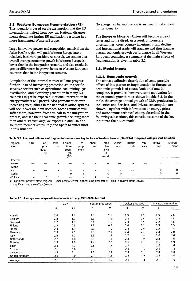
3.2. Western European Fragmentation (FS)This scenario is based on the assumption that the EUintegration is halted from now on. National disagree-ments dominate further EU unification, resulting in amore fragmented Western Europe.

Large innovative powers and competition mainly from theAsian Pacific region will push Western Europe into arelatively backward position. As a result, we assume thatoverall average economic growth in Western Europe islower than in the integration scenario, and also results ingreater differences in growth between Western Europeancounties than in the integration scenario.

Completion of the internal market will not progressfurther. Instead increasing protectionism in specificsensitive sectors such as agriculture, coal mining, gasdistribution, and electricity generation in many EU-countries might be expected. National intervention inenergy markets will prevail. Also permanent or evenincreasing inequalities in the national taxation systemswill occur over the next decades. Some countries willsuffer more, however, from this halt in the integrationprocess, and see their economic growth declining morethan others. Particularly, we expect Finland, UK andsouthern member states Italy and Spain to suffer mostin this situation.

No energy tax harmonisation is assumed to take placein this scenario.

The European Monetary Union will become a deadletter and not realised. As a result of monetaryuncertainties, cross-country investments will declineand international trade will stagnate and thus hamperoverall economic growth performance in all WesternEuropean counties. A summary of the main effects offragmentation is given in table 3.2

3.3. Model inputs

3.3.1. Economic growthThe above qualitative description of some possibleeffects of integration or fragmentation in Europe oneconomic growth is of course both brief and in-complete. It provides, however, some motivation forthe economic growth rates shown in table 3.3. In thetable, the average annual growth of GDP, production inIndustries and Services, and Private consumption areshown. Together with information on energy pricesand autonomous technical change described in thefollowing subsections, this constitutes some of the keyinput into the SEEM model.

Table 3.2. Assumed influence of fragmentation on some key factors in Western Europe (EU+EFTA) compared with present situation

Fragmen- GDP Ind. Prod. Compe

Em- Labour

Trade

Energy Interest

Pros- Innova- Environ-tation pro- cost

titive ploy- cost

ba- prices rate perity tion ment

ducti- stren- ment

lance

on gth

EC-

(EC)

World- Internalmarket- Mone-tary- Social- Political 0 0

00

0 0++

++ significant positive effect (higher). + small positive effect (higher). 0 no clear effect. - small negative effect (lower).- significant negative effect (lower).

Table 3.3. Average annual growth in economic activity. 1991-2020. Per cent

GDP Industry production Services production Private consumption

IS FS IS FS IS FS IS FS

Austria 2.4 2.1 2.4 2.1 2.5 2.2 2.5 2.0Belgium 2.3 1.9 2.3 1.9 2.4 2.0 2.4 1.8Denmark 2.2 1.8 2.1 1.6 2.3 1.9 2.2 1.6Finland 2.3 0.5 2.3 0.5 2.4 0.5 2.3 0.5France 2.3 1.9 2.3 1.9 2.4 2.0 2.3 1.8Germany 2.3 2.1 2.3 2.1 2.4 2.2 2.4 2.0Italy 2.6 1.7 2.5 1.7 2.7 1.8 2.6 1.6Netherlands 2.2 1.8 2.1 1.6 2.3 1.9 2.2 1.6Norway 2.4 2.0 2.4 2.0 2.5 2.1 2.5 1.9Spain 2.6 1.7 2.5 1.7 2.7 1.8 2.6 1.6Sweden 2.3 1.6 2.3 1.6 2.4 1.5 2.4 1.4Switzerland 2.3 2.1 2.3 2.1 2.4 2.2 2.4 2.0United Kingdom 2.2 1.0 2.1 1.1 2.3 1.0 2.1 1.0

Average 2.3 1.7 2.3 1.7 2.4 1.8 2.4 1.6

13

1991 USDper toe

240 -

200 -

160 -

120 -

80 -

40 -

0

1991

- - - -oil-is gas-is

--A-- - oil-fs

coal

1995 2000 2005 2010 2015

gas-fs

A -----A


3.3.2. Energy pricesIn the integration scenario we assume that a successfuleconomic transition in Russia will take place and thatthis will keep oil and gas prices low. Together with thestructural developments in Western Europe this willlead to decreasing gas prices. At about 2005 the gasprice is expected to be uncoupled from the oil price.However in the fragmentation scenario, we assume amonotonic, but modest, increase in oil and gas prices,due to lack of new investments and thus exports fromRussia. After about 2015 the resulting gas prices reachvalues above oil prices from the Middle East.

Figure 3.1 shows the development in oil and gas importprices according to the two scenarios. We assume thatthe coal import price for EU countries will remainstable at the present price level in both scenarios.

Figure 3.1. Fossil fuel import prices. Average over SEEMcountries

Table 3.4. Annual change in autonomous technical efficiency.1991-2020. Per cent

Services Households

IS 0.6 0.4 0.4FS 0.3 0.2 0.2

Industry

3.3.3. Autonomous efficiency improvementOur assumptions on autonomous efficiency improve-ment are rather conservative in both scenarios, due torelative low prices in the integration scenario and alack of co-operation in the fragmentation scenario. Ingeneral, efficiency improvement in IS is expected to belarger than in FS, because of higher economic growth,thus inducing faster turnover and more competition.Furthermore, it is expected that industry is moreefficiency oriented, thus more improvement can berealised here than in services or households.

In southern countries like Spain and Italy it is expectedthat the starting situation lags behind Western Euro-pean averages. Therefore, in these countries annuallyrealised efficiency improvements can be relatively high-er, particularly in industry. Summarising, table 3.4shows the country averages of the autonomousefficiency improvements adopted in the simulations.

14


4. Simulation results

4.1. Energy demandIn the presentation of the simulation results, we firstconcentrate on demand for the endogenously deter-mined fossil fuels. Nuclear and renewable energy useare mostly exogeneously given in the two scenarios.

The development in fossil fuel consumption can besummarily explained by changes in:• economic activity• technological improvements• fuel import prices• fuel taxes

The relative impacts of these factors in going from theintegration (IS) to the fragmentation (FS) scenario isshown in table 4.1.

Table 4.1. Impacts on energy consumption of various factors ingoing from IS to FS

Oil Gas Coal Total

Economic growth _ _

Technology + +Fuel import prices _ _

Fuel tax harmonisation + —

Total

(+ indicates higher fuel demand in FS than in IS)

Since we have assumed a higher economic activitygrowth in IS than in FS (approximately 2.3 per cent peryear vs. 1.7 per cent), this tends to lower the demandfor all fuels in FS compared to IS. This is marked byin the table. The technology assumptions work theopposite way. We have assumed higher (autonomous)energy savings and fuel efficiency improvements in theintegration scenario (see table 3.4), implying that, atconstant fuel prices, the energy intensity will becomehigher in FS, i.e. more fuel is used per output ("+" inthe table). Roughly speaking, the activity effect and thetechnology effect tend to more or less offset each otherwhen it comes to the overall effect on total fueldemand.

From figure 3.1 it is clear that the oil and gas prices arelower in the integration scenario than in the frag-mentation scenario, resulting in lower oil and gasconsumption in FS than in IS. The price differences areespecially high for oil from 2005, so the effects havetime to work out completely despite lag effects in themodel. This results in a double "—" for the oil demanddifference between FS and IS in the table. Although thecoal import price stays constant in both scenarios, it ismore favourable compared to oil and gas prices in theFS scenario. Thus, the fuel price effect is that coaldemand is higher in FS than in IS.

The fourth major difference in input between thescenarios is the tax harmonisation implemented in theintegration scenario. Due to extremely high taxes onnatural gas used in households in some countrieswhere gas consumption is high (Italy is the mainexample), removal of the harmonisation leads toreduced gas consumption at the aggregate level. Theeffect on oil is opposite (but weak), mainly becausesome of the large countries today have gasoline taxesslightly below the average of the four big countries.Overall, the effect of the tax harmonisation must beconsidered to be weak.

Summing up the separate effects, as shown by thebottom line of the table, the net effect of the differentscenario inputs is that the demand for oil, gas and totalenergy demand, is higher in the IS scenario than in theFS scenario. Altered input assumptions could of coursechange these results. For instance, a higher rate oftechnology improvement in the integration scenariowould reduce the gap between total fuel demand in ISand FS.

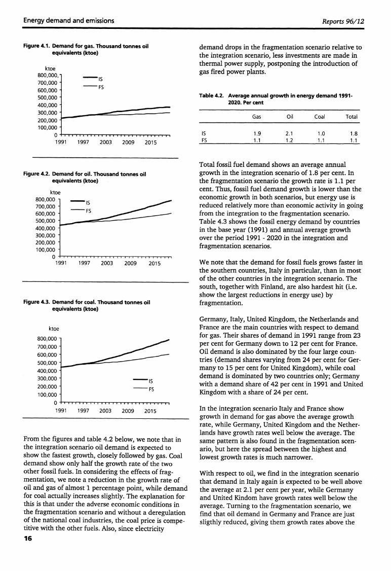
The figures 4.1 - 4.3 show the simulated time paths ofaggregated demand for natural gas, oil and coal in theintegration (IS) and fragmentation scenarios.

0 0

15

800,000 -700,000 -600,000 -500,000 -400,000 -300,000 -200,000 -100,000 -

0 -

1991 1997 2003 2009 2015

IS- FS

1 1 111


Figure 4.1. Demand for gas. Thousand tonnes oilequivalents (ktoe)

ktoe800,000, -700,000 -600,000 -500,000 -400,000 -300,000 -200,000:100,000 -

11111111111111111111111-1111

1991 1997 2003 2009 2015

Figure 4.2. Demand for oil. Thousand tonnes oilequivalents (ktoe)

ktoe800,000 -700,000 -600,000 -500,000 -400,000 -300,000 -200,000 -100,000 -

0 - 1991

Figure 4.3. Demand for coal. Thousand tonnes oilequivalents (ktoe)

ktoe

From the figures and table 4.2 below, we note that inthe integration scenario oil demand is expected toshow the fastest growth, closely followed by gas. Coaldemand show only half the growth rate of the twoother fossil fuels. In considering the effects of frag-mentation, we note a reduction in the growth rate ofoil and gas of almost 1 percentage point, while demandfor coal actually increases slightly. The explanation forthis is that under the adverse economic conditions inthe fragmentation scenario and without a deregulationof the national coal industries, the coal price is compe-titive with the other fuels. Also, since electricity

demand drops in the fragmentation scenario relative tothe integration scenario, less investments are made inthermal power supply, postponing the introduction ofgas fired power plants.

Table 4.2. Average annual growth in energy demand 1991-2020. Per cent

Gas Oil Coal Total

IS 1.9 2.1 1.0 1.8FS 1.1 1.2 1.1 1.1

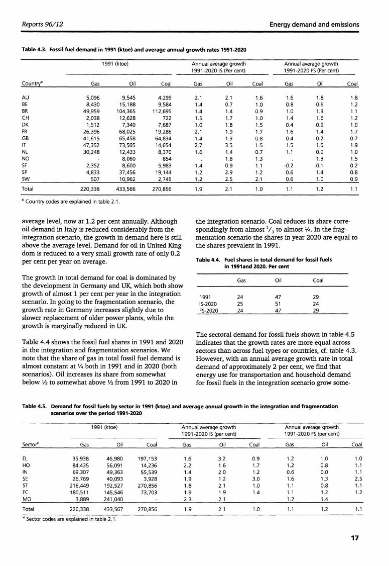
Total fossil fuel demand shows an average annualgrowth in the integration scenario of 1.8 per cent. Inthe fragmentation scenario the growth rate is 1.1 percent. Thus, fossil fuel demand growth is lower than theeconomic growth in both scenarios, but energy use isreduced relatively more than economic activity in goingfrom the integration to the fragmentation scenario.Table 4.3 shows the fossil energy demand by countriesin the base year (1991) and annual average growthover the period 1991 - 2020 in the integration andfragmentation scenarios.

We note that the demand for fossil fuels grows faster inthe southern countries, Italy in particular, than in mostof the other countries in the integration scenario. Thesouth, together with Finland, are also hardest hit (i.e.show the largest reductions in energy use) byfragmentation.

Germany, Italy, United Kingdom, the Netherlands andFrance are the main countries with respect to demandfor gas. Their shares of demand in 1991 range from 23per cent for Germany down to 12 per cent for France.Oil demand is also dominated by the four large coun-tries (demand shares varying from 24 per cent for Ger-many to 15 per cent for United Kingdom), while coaldemand is dominated by two countries only; Germanywith a demand share of 42 per cent in 1991 and UnitedKingdom with a share of 24 per cent.

In the integration scenario Italy and France showgrowth in demand for gas above the average growthrate, while Germany, United Kingdom and the Nether-lands have growth rates well below the average. Thesame pattern is also found in the fragmentation scen-ario, but here the spread between the highest andlowest growth rates is much narrower.

With respect to oil, we find in the integration scenariothat demand in Italy again is expected to be well abovethe average at 2.1 per cent per year, while Germanyand United Kindom have growth rates well below theaverage. Turning to the fragmentation scenario, wefind that oil demand in Germany and France are justsligthly reduced, giving them growth rates above the

IS- FS

1111111111111

1997 2003 2009 2015

16


Table 4.3. Fossil fuel demand in 1991 (ktoe) and average annual growth rates 1991-2020

1991 (ktoe) Annual average growth1 991 -2020 IS (Per cent)

Annual average growth1 991 -2020 FS (Per cent)

Country' Gas Oil Coal Gas Oil Coal Gas Oil Coal

AU 5,096 9,545 4,299 2.1 2.1 1.6 1.6 1.8 1.8BE 8,430 15,188 9,584 1.4 0.7 1.0 0.8 0.6 1.2BR 49,959 104,365 112,695 1.4 1.4 0.9 1.0 1.3 1.1CH 2,038 12,628 722 1.5 1.7 1.0 1.4 1.6 1.2DK 1,512 7,340 7,687 1.0 1.8 1.5 0.4 0.9 1.0FR 26,396 68,025 19,286 2.1 1.9 1.7 1.6 1.4 1.7GB 41,615 65,458 64,834 1.4 1.3 0.8 0.4 0.2 0.7IT 47,352 73,505 14,654 2.7 3.5 1.5 1.5 1.5 1.9NL 30,248 12,433 8,370 1.6 1.4 0.7 1.1 0.9 1.0NO - 8,060 854 1.8 1.3 1.3 1.5SF 2,352 8,600 5,983 1.4 0.9 1.1 -0.2 -0.1 0.2SP 4,833 37,456 19,144 1.2 2.9 1.2 0.6 1.4 0.8SW 507 10,962 2,745 1.2 2.5 2.1 0.6 1.0 0.9

Total 220,338 433,566 270,856 1.9 2.1 1.0 1.1 1.2 1.1

a) Country codes are explained in table 2.1.

average level, now at 1.2 per cent annually. Althoughoil demand in Italy is reduced considerably from theintegration scenario, the growth in demand here is stillabove the average level. Demand for oil in United King-dom is reduced to a very small growth rate of only 0.2per cent per year on average.

The growth in total demand for coal is dominated bythe development in Germany and UK, which both showgrowth of almost 1 per cent per year in the integrationscenario. In going to the fragmentation scenario, thegrowth rate in Germany increases slightly due toslower replacement of older power plants, while thegrowth is marginally reduced in UK.

Table 4.4 shows the fossil fuel shares in 1991 and 2020in the integration and fragmentation scenarios. Wenote that the share of gas in total fossil fuel demand isalmost constant at 1/4 both in 1991 and in 2020 (bothscenarios). Oil increases its share from somewhatbelow 1/2 to somewhat above 1/2 from 1991 to 2020 in

the integration scenario. Coal reduces its share corre-spondingly from almost 1/3 to almost 1/4• In the frag-mentation scenario the shares in year 2020 are equal tothe shares prevalent in 1991.

Table 4.4. Fuel shares in total demand for fossil fuelsin 1991and 2020. Per cent

Gas

Oil Coal

1991 24 47 29IS-2020 25 51 24FS-2020 24 47 29

The sectoral demand for fossil fuels shown in table 4.5indicates that the growth rates are more equal acrosssectors than across fuel types or countries, cf. table 4.3.However, with an annual average growth rate in totaldemand of approximately 2 per cent, we find thatenergy use for transportation and household demandfor fossil fuels in the integration scenario grow some-

Table 4.5. Demand for fossil fuels by sector in 1991 (ktoe) and average annual growth in the integration and fragmentationscenarios over the period 1991-2020

1991 (ktoe) Annual average growth1 991 -2020 IS (per cent)

Annual average growth1 991 -2020 FS (per cent)

Sector' Gas Oil Coal Gas Oil Coal Gas Oil Coal

EL 35,938 46,980 197,153 1.6 3.2 0.9 1.2 1.0 1.0HO 84,435 56,091 14,236 2.2 1.6 1.7 1.2 0.8 1.1IN 69,307 49,363 55,539 1.4 2.0 1.2 0.6 0.0 1.1SE 26,769 40,093 3,928 1.9 1.2 3.0 1.6 1.3 2.5ST 216,449 192,527 270,856 1.8 2.1 1.0 1.1 0.8 1.1FC 180,511 145,546 73,703 1.9 1.9 1.4 1.1 1.2 1.2MO 3,889 241,040 2.3 2.1 1.2 1.4

Total 220,338 433,567 270,856 1.9 2.1 1.0 1.1 1.2 1.1

Sector codes are explained in table 2.1.

17

Mill.tonnes

5000 -

4000 '-

3000

2000 -

1000 -

01991

El CoalOil

M Gas

IS-2020 FS-2020

0 South

1111Nordic

CI Small

0 United Kingdom

0 France

• Germany


what faster than demand from the other sectors. Incomparison, industry shows a growth rate of 1.5 percent. In the fragmentation scenario we note that de-mand from the service sector remains relatively un-affected by the scenario assumptions, and displays onlya slight decrease relative to the integration scenario.

The difference in oil demand between IS and FS islargest in the electricity generation sector. This ismainly explained by the low taxes in the integrationscenario, and thus heavily decreasing prices in theelectricity sector. Furthermore, especially in the UK andItaly, a major difference between activity growth isassumed, resulting in a large demand for electricity inIS.

The gap in oil demand in the industry sector betweenIS and FS is also rather large. This can be explained bylow tax rates combined with relatively high elasticities.

For sectoral gas demand the services sector shows onlya small difference between IS and FS. This is due tohigh taxes which dampen the differences in gas importprices between the two scenarios. In the householdsector the tax rates are also relatively high. However,reaction on energy demand is much larger, becauseincome elasticities in that sector are much greater thanin the service sector.

The sectoral demand for coal is dominated by theelectricity generating sector. In contrast to the otherfuels, demand for coal is slightly increased in goingfrom the integration to the fragmentation scenario. Asmentioned before, this is mainly due to a slowerreplacement of old coal fired power plants in thefragmentation scenario.

4.2. Emissions to air

4.2.1. Emission of CO2Emissions of CO, are determined by the carbon contentof each fuel. The emission factors employed in thisstudy are as follows: Gaseous fuels: 2.4, liquid fuels:3.1 and solid fuels: 3.9, all measured in (metric) tonnesof CO, per tonnes oil equivalents (t.o.e.). Figures 4.4 -4.6 show emission levels in 1991 and in year 2020 inthe two scenarios from groups of countries6, by fueltypes and by sectors. Average annual growth in CO,emissions are 1.7 per cent in the integration scenarioand 1.1 per cent in the fragmentation scenario. TotalCO, emissions grow somewhat slower than total de-mand for fossil fuels, since both oil and gas (withrelatively low emission coefficients) grow faster thandemand for coal (with a relatively high emission co-efficient). In the integration scenario Germany reduces

6 The country aggregates are defined by the following labels:Austria, Switzerland, Belgium and the Netherlands are the «Small.countries. The “South” countries consist of Italy and Spain, whilethe «Nordic» countries are Denmark, Finland, Sweden and Norway.

its share of emissions, while Italy increases its share. Inthe fragmentation scenario the 1991-shares are moreor less restored in 2020, expect for United Kingdomwhich reduces its share from 19 per cent to 16 per centin both scenarios.

With respect to type of fuel, we find that the share ofoil related emissions, and to a much smaller extend thegas related emissions, increase in the integration scen-ario, while the base year shares are restored in thefragmentation scenario in 2020.

Electricity generation and transport are the dominatingsectors with respect to CO, emissions. Since transportactivities are assumed to grow relatively fast in bothscenarios, its share increases from 26 per cent in 1991to 29 per cent in year 2020 in the integration scenarioand 28 per cent in the fragmentation scenario. Elec-tricity generation reduces its share from 34 per cent in1991 to 31 and 33 per cent in year 2020 in the IS andFS scenarios, respectively.

Figure 4.4. Emissions of CO, by group of countries

1991

IS- FS-

2020 2020

Figure 4.5. Emissions of CO, by type of fuels

Mill.tonnes5000 -

4000 -

3000 -

2000 -

1000 -

0

18

5000 -4500 -4000 -3500 -3000 -2500 -2000 -1500 -1000 -500 -

0

O M°• SEM IN0 HO• EL

1991 IS-2020

FS-2020

Energy demand and emissionsReports 96/12

Figure 4.6. Emissions of CO, by sectors Figure 4.7. SO2 emissions in 1991 and 2020 by country groups

Mill. tonnesMill. tonnes

SO2

0 South• NordicIN Small

0 United Kingdom0 France

• Germany

35 -30 -25 -20 -15 -10 -5 -0

1991 IS- FS-

2020 2020

4.2.2. Emissions of SO2 and NOUnlike CO, emissions, the emission of SO2 and NOdepends on how the fossil fuels are burned (combus-tion technology) as well as the amount of cleaning ofexhaust gases that takes place. These emissions willtherefore not necessarily follow the pattern of fossilfuel demand. Also, in the case of sulphur emissions,these are dominated by the demand for coal which ismore sulphurous than the other fossil fuels.

As mentioned above, we calculate the emissions of SO2an NO by inserting energy trajectories from the SEEMmodel into IIASA's RAINS model (Alcamo et al. 1990,Kolsrud, 1996). The simulated SEEM figures are suit-ably transformed to take into account differences indefinitions of sectors and fuels between the two mod-els. Utilising the technology assumptions incorporatedin the Official Energy Pathway (OEP) scenario ofRAINS, we can then calculate SO2 and NO emissionsand also use the atmospheric transport module to findthe deposition pattern associated with our energyscenarios'.

Total SO2 emissions are growing at an annual averagerate of 1.3 per cent in the integration scenario versusonly 0.5 per cent in the fragmentation scenario, seefigure 4.7. These comparatively low growth rates aredue to the fact that SO2 emissions from Germany aredeclining in both scenarios. This is explained by theforecasted large reduction in coal used in the eastern

7 As explained in Alfsen et al. (1995) and Kolsrud (1996), SEEMdoes not provide values for all the energy variables entering theRAINS model. In addition, the Official Energy Pathway scenario ofthe RAINS model, that provides the technology parameters relevantto the SO2 and NO emission calculations, has a time horizon to year2000. After this time, we have kept the technology parametersconstant in our simulations. This allows us to study the partialeffects of changing energy consumption pattern, and to interpret theresults in purely economic terms. Furthermore, the energy variablesnot provided by SEEM are forecasted using total demand for solid,liquid and gaseous fossil fuels simulated by SEEM as relevantindicators.

Figure 4.8 NO, emissions in 1991 and 2020 by country groups

Mill. tonnesNO2

30 -

25 -

20

15 -

10 -

5 -

0 1991 I5-2020 FS-2020

part of the country. The other big contributer to SO2emissions is the southern block, i.e. Italy and Spain.

High economic growth rates in the integration scenariolead to high emissions. In 2020 their combined emis-sion share is almost 40 per cent, up from 28 per cent inthe base year 1991. Even in the fragmentation scen-ario, where their economic growth is closer to the aver-age growth of all countries, Italy and Spain increasetheir share of SO2 emissions from 28 per cent to 32 percent.

Total NO emissions grow more in line with total ener-gy demand, see figure 4.8. While SO, emissions weredetermined by the use of coal and oil primarily in thepower producing sector, transport oil use is an impor-tant determinant for the NO emissions. The southerncountries also in this case increase their shares of emis-sions from 20 per cent in 1991 to 30 per cent in 2020in the integration scenario and more modestly to 23per cent in the fragmentation scenario.

Further information on the SO2 and NO emissions aregiven in the tables 4.6 and 4.7. Both oil and coal usecontribute significantly to the SO2 emissions. The coaluse is not much affected by neither integration nor

OSouth

• Nordic

El Small

CI United Kingdom

El France

Germany

19

SO2emis-sions.

Shares1991

Average annualgrowth

1991-2020

NOemis-sions.

Shares1991

Averageannual growth

1991-2020IS FS IS FS

Conver-sion 8 2.9 1.2 2 2.3 1.2Powerprod. 68 1.0 0.4 21 1.1 0.7Domestic 10 1.4 0.4 5 1.8 1.1Traffic 3 2.6 1.6 65 2.1 1.5Industry 11 1.7 0.3 6 1.5 0.7

Total 100 1.3 0.5 100 1.7 1.2

O South

M Nordic

III Small• United Kingdom0 France• Germany


fragmentation, and coal emissions grow in both scen-arios at a modest average rate close to 0.1 per cent peryear. Oil contributes more to SO2 and NO emissions inthe future than in 1991 in both scenarios, but mostprominently in the integration scenario. From table 4.7we note that most of the SO2 emissions are comingfrom the power producing sector, and that this is thecase also in the future in both scenarios although othersectors' contribution are likely to grow somewhat.

in the SEEM countries coming from the SEEM coun-tries. Table 4.8 shows the average annual growth rates.The figures 4.9 and 4.10 show the deposition of oxi-dised sulphur and nitrogen in groups of SEEM coun-tries coming from these same groups in 1991 and in2020.

Table 4.8. Average annual growth rates in deposition ofoxidised sulphur and nitrogen. 1991-2020. Per cent

Table 4.6. Shares om emissions in 1991 and average annualgrowth rates from 1991 to 2020 in the integration(IS) and the fragmentation (FS) scenarios by fueltype. Per cent

SO2 NO

ISFS

1.40.5

1.81.2

SO2, emis-

sions


1991-2020

NOemis-sions

Shares1991


1 991 -2020Shares

1991IS FS IS FS

Gas - - 5 1.7 1.0Oil 36 2.9 1.0 71 2.2 1.4Coal 61 0.1 0.2 20 0.7 0.8Othera 4 0.2 0.0 3 -0.1 -0.1

Total 100 1.3 0.5 100 1.7 1.2

Other includes emissions from non-combustion processes and from use ofalternative technologies.

The use of oil is the most prominent cause of NO emis-sions in the SEEM countries, in particular for transportpurposes. The dominant role of transport is likely to in-crease in the future.

Table 4.7 Shares om emissions in 1991 and average annualgrowth rates from 1991 to 2020 in the integration(IS) and the fragmentation (FS) scenarios by RAINS'sectors. Per cent

Figure 4.9 Sulphur deposition in 1991 and 2020

Mill. tonnesSO2

20 -

O South

• Nordic

0 Small

United Kingdom

0 France

• Germany

1991 I5-2020

FS-2020

Figure 4.10 Nitrogen deposition in 1991 and 2020

Mill. tonnesNO2

15 -

10 -

5 - VX,1 rOM

4.2.3. Deposition of SO2 and NOR-Deposition of sulphur and oxidised nitrogen is calcu-lated using the above emission figures and the tran-sport matrices for 1991, as given by Sandnes (1993).The SEEM countries only constitute a subset of thecountries covered by RAINS and the transport matrices.Here we only consider the contribution to depositions

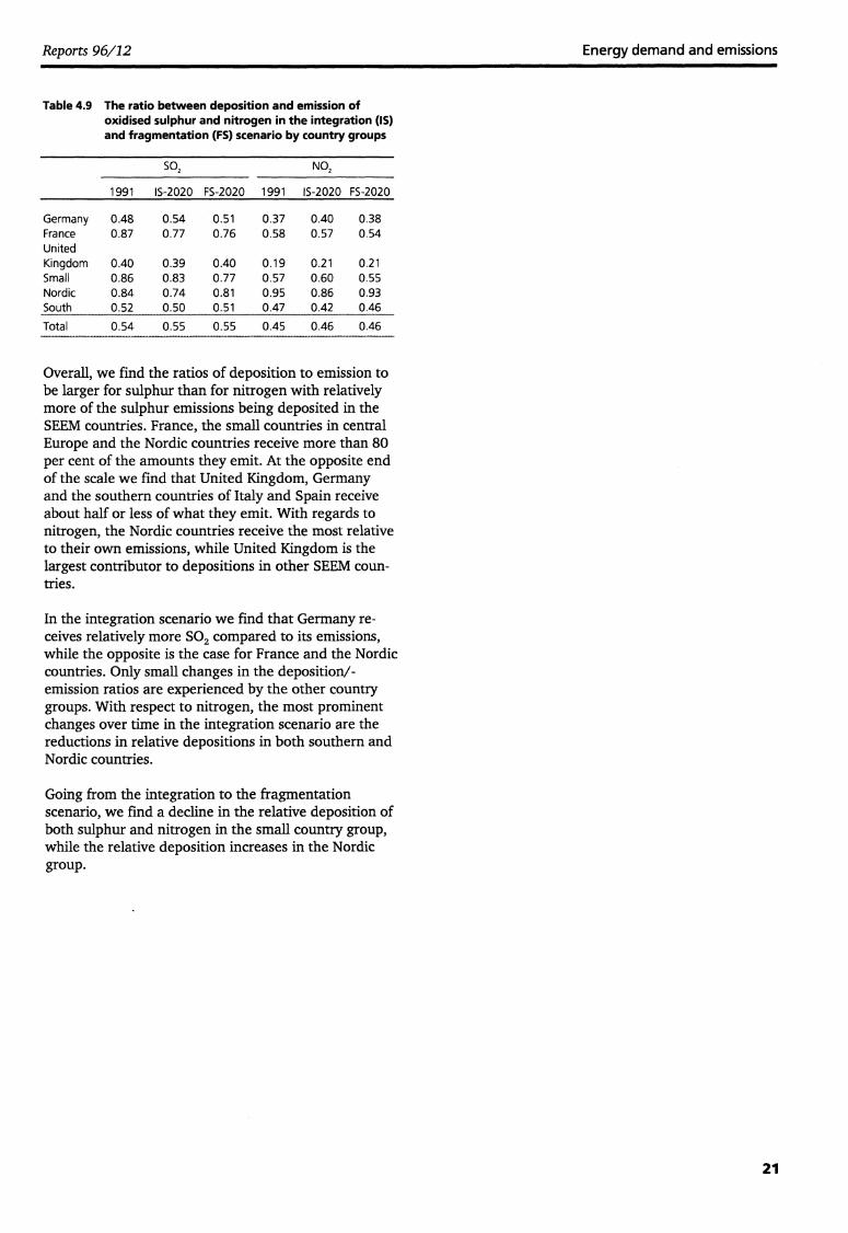
Table 4.9 show how the ratio between depositions andemissions develop from 1991 to 2020 in the twoscenarios.

20


Table 4.9 The ratio between deposition and emission ofoxidised sulphur and nitrogen in the integration (IS)and fragmentation (FS) scenario by country groups

SO, NO2

1991 15-2020 FS-2020 1991 I5-2020 FS-2020

Germany 0.48 0.54 0.51 0.37 0.40 0.38France 0.87 0.77 0.76 0.58 0.57 0.54UnitedKingdom 0.40 0.39 0.40 0.19 0.21 0.21Small 0.86 0.83 0.77 0.57 0.60 0.55Nordic 0.84 0.74 0.81 0.95 0.86 0.93South 0.52 0.50 0.51 0.47 0.42 0.46

Total 0.54 0.55 0.55 0.45 0.46 0.46

Overall, we find the ratios of deposition to emission tobe larger for sulphur than for nitrogen with relativelymore of the sulphur emissions being deposited in theSEEM countries. France, the small countries in centralEurope and the Nordic countries receive more than 80per cent of the amounts they emit. At the opposite endof the scale we find that United Kingdom, Germanyand the southern countries of Italy and Spain receiveabout half or less of what they emit. With regards tonitrogen, the Nordic countries receive the most relativeto their own emissions, while United Kingdom is thelargest contributor to depositions in other SEEM coun-tries.

In the integration scenario we find that Germany re-ceives relatively more SO2 compared to its emissions,while the opposite is the case for France and the Nordiccountries. Only small changes in the deposition/-emission ratios are experienced by the other countrygroups. With respect to nitrogen, the most prominentchanges over time in the integration scenario are thereductions in relative depositions in both southern andNordic countries.

Going from the integration to the fragmentationscenario, we find a decline in the relative deposition ofboth sulphur and nitrogen in the small country group,while the relative deposition increases in the Nordicgroup.

21


5. Conclusion

Several models in the literature have analysed energyscenarios for Western Europe, e.g. Global 2100 (Manneand Richels, 1992), GREEN (Bumiaux et al., 1992) andECON-ENERGY (Haugland et al., 1992). However, inthese models Western Europe is treated as one block.In contrast, the SEEM model is more detailed, since itmodels energy demand and emissions to air from eachof the countries covered. The SEEM model is alsounique in that it allows for a linkage to the RAINSmodelling system.

The SEEM simulations in this paper have been basedon two exogenously given economic growth scenarioswith the following main features:

• The economy shows only modest growth in the inte-gration scenario, strongest in the southern part ofEurope. The growth rate is even lower in thefragmentation scenario. The southern countriesexperience the largest reduction in economicgrowth, while the growth in Germany is almostunaffected in going from the integration to thefragmentation scenario.

With respect to the issues addressed in this paper, i.e.the effect of integration or fragmentation in Europe onfuture energy demand, emissions to air and depositionof acid compounds, the simulations indicate that:

• Overall the demand for fossil fuels grows at an ave-rage annual rate of 1.8 per cent in the integrationscenario and 1.1 per cent in the fragmentation scen-ario. Average annual growth in demand for oil andgas in the integration scenario is around 2 per centper year, while demand for coal grows at a rateclose to 1 per cent per year. In the fragmentationscenario the demand for coal is slightly higher,while the average annual growth in demand for oiland gas is reduced to approximately 1 per cent.

• Growth in CO, emissions follows the growth inoverall demand for fossil fuels. The power gene-rating sector and transport are the two most contri-butors to CO, emissions, each with an emissionshare of around 30 per cent.

• SO, emissions are dominated by oil and coal use inthe power generating sector. Italy, United Kingdomand Germany are the largest contributers. Theaverage annual growth in total 502 emissions in theintegration and the fragmentation scenarios are 1.3and 0.5 per cent, respectively. The stronger growthin the integration scenario is due to higher demandfor oil.

• NO emissions are more evenly distributed amongthe countries, and is strongly dominated byemissions from transportation. This is also thesector with the strongest economic growth. Overallwe find that the average annual growth in NOemissions are close to the growth in demand forfossil fuels and CO, emissions, i.e. 1.7 and 1.2 percent in the integration and the fragmentationscenario, respectively.

• With regard to depositions of 502 and NO., theyfollow the emission pattern quite closely, with slowor no growth in sulphur deposition in Germany andrelatively high growth in the southern countries.Growth in nitrogen depositions are more evenlydistributed among the countries.

With respect to further work, we would like to pointout the following. The data used for estimating andcalibrating elasticities and other parameters in themodel can always be improved. Furthermore, themodel's treatment of energy trade is simplistic. Finally,being a partial energy model, SEEM lacks explicitmodelling of the linkages to economic growth. Furtherwork in all of these areas could improve the ability ofthe model apparatus to address the many futurechallenges facing EU and neighbouring countries inEurope in the years ahead.

22


References

Alcamo, J., R. Shaw and L. Hoordijk (eds.) (1990): TheRAINS model of acidification. Science and strategies inEurope, Kluwer Academic Publishers, Dordrecht.

Alfsen, K. H., H. Birkelund and M. Aaserud (1995):Impact of an EC carbon/energy tax and deregulatingthermal power supply on CO,, SO2 and NO emissions,Environmental and Resource Economics 5, 165-189.

Birkelund, H., E. Gjelsvik and M. Aaserud (1993):Carbon/energy tax and the energy market in WesternEurope, Discussion papers 81, Statistics Norway, Oslo.

Birkelund, H., E. Gjelsvik and M. Aaserud (1994): TheEU carbon/energy tax: Effects in a distorted energymarket, Energy Policy 22, 657-665.

Boug, P. (1995): User's Guide. The SEEM modelversion 2.0, Documents 95/6, Statistics Norway, Oslo.

Boug, P., and L. Brubakk (1996): Impacts of economicintegration on energy demand and CO, emissions inWester Europe, to appear in the series Discussionpapers, Statistics Norway, Oslo.

Brubakk, L., M. Aaserud, W. Pellekaan and F. vanOostvoorn (1995): SEEM - An energy demand modelfor Western Europe, Reports 95/24, Statistics Norway,Oslo.

Burniaux, J. M., J. P. Martin, G. Nicoletti and J.Oliviera Martins (1992): GREEN - A multi-regiondynamic general equilibrium model for quantifying thecosts of curbing CO, emissions: A technical manual,Working Paper 116, OECD Economics Department,Paris.

Haugland, T., 0. Olsen and K. Roland (1992):Stabilizing CO, emissions: Are carbon taxes a viableoption?, Energy Policy 20, 405-419.

TEA (International Energy Agency) (1993a): Energybalances in the OECD countries. 1960-1991, IEA, Paris.

IEA (International Energy Agency) (1993b): Energyprices and taxes, IEA, Paris.

Kolsrud, D. (1996): Documentation of computerprograms that extend the SEEM model and provides alink to the RAINS model, Documents 96/1, StatisticsNorway, Oslo.

Manne A., and R. Richels (1992): Buying greenhouseinsurance - The economic costs of CO2 emission limits,MIT Press, Cambridge, Massachusetts.

Sandnes, H. (1993): Calculated budgets for airborne,acidifying components in Europe 1985,1987, 1988,1990, 1991 and 1992. EMEP/MSC-W Report 1/93,Oslo.

23


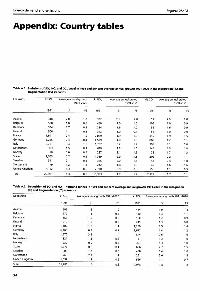
Appendix: Country tables

Table A.1 Emissions of SO2, NO and COP. Level in 1991 and per cent average annual growth 1991-2020 in the integration (IS) andfragmentation (FS) scenarios

kt SO2

1991

Average annual growth1 991 -2020

kt NO2

1991

Average annual growth1 991 -2020

Mt CO, Average annual growth1991-2020

IS FS IS FS 1991 IS FS.

348 2.0 1.8 332 2.1 2.0 59 2.0 1.8538 1.0 0.6 480 1.0 1.0 105 1.0 0.9334 1.7 0.8 284 1.6 1.0 56 1.6 0.9506 1.1 0.3 312 1.0 0.1 56 1.0 0.0

1,641 2.4 1.5 2,089 1.9 1.6 349 1.9 1.58,225 -0.4 -0.4 4,579 1.0 1.0 883 1.2 1.13,761 3.4 1.6 1,737 3.2 1.7 399 3.1 1.6

393 1.5 0.9 639 1.3 1.0 144 1.3 1.090 0.6 0.4 287 2.1 1.9 28 1.7 1.3

2,563 0.7 -0.2 1,359 2.9 1.5 202 2.2 1.1311 2.1 0.3 325 2.0 1.1 46 2.4 1.0

79 1.2 1.1 242 1.8 1.8 47 1.6 1.64,132 1.3 0.6 2,728 0.9 0.3 556 1.1 0.5

22,921 1.3 0.5 15,393 1.7 1.2 2,929 1.7 1.1

Emissions

AustriaBelgiumDenmarkFinlandFranceGermanyItalyNetherlandsNorwaySpainSwedenSwitzerlandUnited Kingdom

Total

Table Al Deposition of SO2 and NOR. Thousand tonnes in 1991 and per cent average annual growth 1991-2020 in the integration(IS) and fragmentation (FS) scenarios

kt SO, Average annual growth 1 991 -2020 kt NO, Average annual growth 1 991 -2020

1991 IS FS 1991 IS FS

502 1.6 1.0 414 1.9 1.4279 1.2 0.8 140 1.4 1.1151 1.0 0.5 100 1.2 0.9319 1.0 0.2 245 1.3 0.8

1,482 1.9 1.1 1,230 1.9 1.46,463 0.8 0.7 1,677 1.4 1.21,876 3.2 1.4 844 2.6 1.6

321 1.2 0.8 181 1.3 1.0230 0.9 0.4 337 1.3 1.0

1,378 0.8 -0.1 696 2.7 1.5380 1.2 0.3 458 1.4 1.0268 2.1 1.1 231 2.0 1.5

1,639 1.3 0.6 526 1.1 0.7

15,286 1.4 0.8 7,078 1.8 1.2

Deposition

AustriaBelgiumDenmarkFinlandFranceGermanyItalyNetherlandsNorwaySpainSwedenSwitzerlandUnited Kingdom

Sum

24


Tidligere utgitt pa emneomrficietPreviously issued on the subject

Documents95/6 P. Boug: User's Guide. The SEEM-model Version

2.0.

96/1 D. Kolsrud: Documentation of ComputerPrograms that Extend the SEEM Model andProvide a Link to the RAINS Model

Rapporter (RAPP)95/24 L. Brubakk, M. Aaserud, W. Pellekaan og F. van

Oostvoorn: An Energy Demand Model forWestern Europe

Okonomiske analyser (OA)8/94 K.H. Alfsen og M. Aaserud: Klimapolitkk,

kraftproduksjon og sur nedbor. Noensimuleringsresultater fra den flersektorelleeuropeiske energimodellen SEEM

Economic Survey (ES)3/93 H. Birkelund, E. Gjelsvik og M. Aaserud: Effects

of an EC Carbon/Energy Tax in a DistortedEnergy Market

Discussion Papers (DP)81 H. Birkelund, E. Gjelsvik and M. Aaserud:

Carbon/Energy Tax and the Energy Market inWestern Europe

104 K.H. Alfsen, H. Birkelund and M. Aaserud:Secondary Benefits of the EC Carbon/EnergyTax

25


De sist utgitte publikasjonene i serien RapporterRecent publications in the series Reports

95/20 R.H. Kitterod: Tid nok, - men hva sa? Tidsbrukog tidsopplevelse blant langtids-arbeidsledige.1995. 123s. 110 kr. ISBN 82-537-4177-4

95/21 N. Keilman and H. Brunborg: HouseholdProjections for Norway, 1990-2020 Part I:Macrosimulations. 1995. 82s. 95 kr. ISBN 82-537-4178-2

95/22 R.H. Kitterod: Tidsbruk og arbeidsdeling blantnorske og svenske foreldre. 1995. 100s. 110 kr.ISBN 82-537-4179-0

95/23 H. Rudlang: Bruk av edb i skolen 1995. 1995.77s. 95 kr. ISBN 82-537-4181-2

95/24 L. Brubakk, M. Aaserud, W. Pellekaan andF. van Oostvoom: SEEM - An Energy DemandModel for Western Europe. 1995. 66s. 95 kr.ISBN 82-537-4185-5

95/25 H. Luras: Framskriving av miljoindikatorer.1995. 30s. 80 kr. ISBN 82-537-4186-3

95/26 G. Frengen, F. Foyn and R. Ragnarson: Inno-vation in Norwegian Manufacturing and OilExtraction in 1992. 1995. 93s. 95 kr. ISBN 82-537-4189-8

95/27 K.H. Alfsen, B.M. Larsen og H. Vennemo:Bwrekraftig Økonomi? Noen alternativemodellscenarier for Norge mot ar 2030. 1995.62s. 95 kr. ISBN 82-537-4190-1

95/28 L.S. Storni*: Flytting og arbeidsstyrken:Flyttetilboyelighet og flyttemonster hosarbeidsledige og sysselsatte i perioden 1988-1993. 1995. 66s. 95 kr. ISBN 82-537-4193-6

95/29 G. Dahl, E. Flittig, J. Lajord og D. Fredriksen:Trygd og velferd. 1995. 91s. 95 kr. ISBN 82-537-4198-7

95/30 T. Skjerpen: Seasonal Adjustment of First TimeRegistered New Passenger Cars in Norway byStructural Time Series Analysis. 1995. 35s. 80kr. ISBN 82-537-4200-2

95/31 A. Bnivoll og K. Ibenholt: Norske avfalls-mengder etter artusenskiftet. 1995. 41s. 80 kr.ISBN 82-537-4208-8

95/32 S. Blom: Innvandrere og bokonsentrasjon i Oslo.1995. 125s. 95 kr. ISBN 82-537-4211-8

95/33 T.A. Johnsen og B.M. Larsen: Kraftmarkeds-modell med energi- og effektdimensjon. 1995.54s. 95 kr. ISBN 82-537-4212-6

95/34 F. R. Aune: Virkninger pa de nordiske energi-markedene av en svensk kjemekraftutfasing.1995. 58s. 95 kr. ISBN 82-537-4213-4

95/35 M.S. Bjerkseth: Engroshandelen i Norge 1985-1992. 1995. 43s. 95 kr. ISBN 82-537-4214-2

95/36 T. Komstad: Vridninger i lonnstakemes relativebrukerpriser pa bolig, ikke-varige goder og fritid1985/86 til 1992/93. 1995. 35s. 80 kr. ISBN 82-537-4216-9

95/38 G.J. Limperopoulos: Usikkerhet i oljeprosjekter.1995. 72s. 95 kr. ISBN 82-537-4222-3

96/1 E. Bowitz, N.O. Mwhle, V.S. Sasmitawidjaja andS.B. Widoyono: MEMLI - The Indonesian Modelfor Environmental Analysis: TechnicalDocumentation. 1996. 70s. 95 kr. ISBN 82-537-4223-1

96/2 A. Essilfie: Investeringer, kostnader og gebyrer iden kommunale avlopssektoren: Resultater fraundersokelsen i 1995. 1996. 36s. 80 kr. ISBN82-537-4239-8

96/3 Resultatkontroll jordbruk 1996: Gjennomforingav tiltak mot forurensninger. 1996. 85s. 95 kr.ISBN 82-537-4244-4

96/4 A. Osmunddalen og T. Kalve: Bofasteinnvandreres bruk av sosialhjelp 1987-1993.1996. 33s. 80 kr. ISBN 82-537-4245-2

96/5 S. Blom: Inn i samfunnet? Flyktningkull iarbeid, utdanning og pa sosialhjelp. 1996. 84s.95 kr. ISBN 82-537-4249-5

96/6 J.E. Finnvold: Kommunale helsetilbud:Organisering, ulikhet og kontinuitet. 1996. 70s.95 kr. ISBN 82-537-4221-5

96/8 K.E. Rosendahl: Helseeffekter av luft-forurensning og virkninger pg okonomiskaktivitet: Generelle relasjoner med anvendelsepa Oslo. 1996. 40s. 80 kr. ISBN 82-537-4277-0

96/12 K.H. Alfsen, P. Boug and D. Kolsrud: Energydemand, carbon emissions and acid rain.Consequences of a changing Western Europe.1996. 26s. 80 kr. ISBN 82-537-4285-1

26

Returadresse:Statistisk sentralbyr.5Postboks 8131 Dep.N-0033 Oslo

Publikasjonen kan bestilles fra:

Statistisk sentralbyraSalg-og abonnementservicePostboks 8131 Dep.N-0033 Oslo

Telefon: 22 00 44 80Telefaks: 22 86 49 76

eller:Akademika — avdeling foroffentlige publikasjonerMollergt. 17Postboks 8134 Dep.N-0033 Oslo

Telefon: 22 11 67 70Telefaks: 22 42 05 51

ISBN 82-537-4285-1ISSN 0806-2056

Pris kr 80,00

Statistisk sentralbyrà410 Statistics Norway

z