Embed Size (px)
Citation preview
KL −KS mass difference from Lattice QCD
Jianglei Yu
Submitted in partial fulfillment of the
requirements for the degree
of Doctor of Philosophy
in the Graduate School of Arts and Sciences
COLUMBIA UNIVERSITY
2014

c©2014
Jianglei Yu
All Rights Reserved
Abstract
KL −KS mass difference from Lattice QCD
Jianglei Yu
The KL − KS mass difference is a promising quantity to reveal new phenomena which
lie outside the standard model. A state-of-art perturbation theory calculation has been
performed at next-to-next-to-leading order (NNLO) and a 40% error is quoted in the final
result. We develop and demonstrate non-perturbative techniques needed to calculate the
KL−KS mass difference, ∆MK , in lattice QCD and carry out exploratory calculations. The
calculations are performed on a 2+1 flavor, domain wall fermion, 163×32 ensemble with a 421
Mev pion and a 243×64 lattice ensemble with a 330 MeV pion. In the 163 lattice calculation,
we drop the double penguin diagrams and the disconnected diagrams. The short distance
part of the mass difference in a 2+1 flavor calculation contains a quadratic divergence cut off
by the lattice spacing. Here, this quadratic divergence is eliminated through the Glashow-
Iliopoulos-Maiani (GIM) mechanism by introducing a quenched charm quark. We obtain a
mass difference ∆MK which ranges from 6.58(30) × 10−12 MeV to 11.89(81) × 10−12 MeV
for kaon masses varying from 563 MeV to 839 MeV. On the 243 lattice, we include all the
diagrams and perform a full calculation. Our result is for a case of unphysical kinematics
with pion, kaon and charmed quark masses of 330, 575 and 949 MeV respectively. We
obtain ∆MK = 3.19(41)(96)× 10−12 MeV, quite similar to the experimental value. Here the
first error is statistical and the second is an estimate of the systematic discretization error.
An interesting aspect of this calculation is the importance of the disconnected diagrams, a
dramatic failure of the OZI rule.
Contents
List of Tables iii
List of Figures vii
Acknowledgments xx
1 Introduction 1
2 Kaon Mixing in the Standard Model 6
2.1 K0 −K0Mixing . . . . . . . . . . . . . . . . . . . . . . . . . . . . . . . . . 6
2.2 Perturbation Theory Calculation for ∆MK . . . . . . . . . . . . . . . . . . . 10
3 K0-K mixing from Lattice QCD 15
3.1 Second Order Weak Amplitude . . . . . . . . . . . . . . . . . . . . . . . . . 15
3.2 Diagrams Needed for the Lattice Calculation . . . . . . . . . . . . . . . . . . 21
3.3 Wilson Coefficients . . . . . . . . . . . . . . . . . . . . . . . . . . . . . . . . 24
3.4 Non-perturbative Renormalization . . . . . . . . . . . . . . . . . . . . . . . . 25
3.5 Short distance correction . . . . . . . . . . . . . . . . . . . . . . . . . . . . . 30
3.6 Finite volume corrections . . . . . . . . . . . . . . . . . . . . . . . . . . . . . 32
4 Measurement methods 36
4.1 Propagator sources . . . . . . . . . . . . . . . . . . . . . . . . . . . . . . . . 36
i
4.2 Low Mode Deflation . . . . . . . . . . . . . . . . . . . . . . . . . . . . . . . 39
4.3 Two-point and three-point correlators . . . . . . . . . . . . . . . . . . . . . . 42
4.4 Evaluation of four-point correlators . . . . . . . . . . . . . . . . . . . . . . . 43
4.5 Data Analysis . . . . . . . . . . . . . . . . . . . . . . . . . . . . . . . . . . . 45
5 Results from the 163 × 32× 16 Lattice 48
5.1 Simulation Details . . . . . . . . . . . . . . . . . . . . . . . . . . . . . . . . 48
5.2 Short Distance Contribution . . . . . . . . . . . . . . . . . . . . . . . . . . . 51
5.3 Long Distance Contribution . . . . . . . . . . . . . . . . . . . . . . . . . . . 55
5.4 The KL −KS Mass Difference from the 163 Lattice . . . . . . . . . . . . . . 58
5.5 Comparison with NLO Perturbative Calculation . . . . . . . . . . . . . . . . 60
6 Results from the 243 × 64× 16 Lattice 64
6.1 Simulation Details . . . . . . . . . . . . . . . . . . . . . . . . . . . . . . . . 64
6.2 The KL −KS Mass Difference from the 243 Lattice . . . . . . . . . . . . . . 65
6.3 Contributions from Different Diagrams . . . . . . . . . . . . . . . . . . . . . 67
6.4 Effects of Scalar and Pseudoscalar Operators . . . . . . . . . . . . . . . . . . 69
7 Conclusions 72
A K0-K0Mixing Contractions 75
Bibliography 77
ii
List of Tables
1 The values of the parameters used in the calculation of Wilson coefficients. . 81
2 The Wilson coefficients, the RI → MS matching matrix, the non-perturbative
lat → RI operator renormalization matrix and their final product, all at a
scale µ = 2.15 GeV shown in columns one through four respectively. . . . . . 81
3 Valence charm quark masses used to implement the GIM cancellation on the
163 lattice. The upper row gives the bare masses in lattice units. The lower
row contains the MS masses at a scale of 2 GeV. . . . . . . . . . . . . . . . . 81
4 Valence strange quark mass (upper row) and kaon mass (lower row) on the
163 lattice, both in lattice units. . . . . . . . . . . . . . . . . . . . . . . . . . 82
5 The values of the parameters used in the EigCG algorithm on the 163 lattice.
The meaning of these parameters are given in Ref. [1, 2]. . . . . . . . . . . . 82
6 The mass difference ∆M11K , defined in Eq. (5.6) after GIM cancellation, eval-
uated for different charm quark masses. These results were obtained on the
163 lattice, use 600 configurations and a kaon mass of 563 MeV and are the
matrix elements of bare lattice operators without Wilson coefficients or renor-
malization factors. . . . . . . . . . . . . . . . . . . . . . . . . . . . . . . . . 82
7 Results for single-pion matrix elements, 〈π0|Qi|K0〉, at various kaon masses
on the 163 lattice. We use π0 = iuγ5u and only include the first two diagrams
in Fig. 11. . . . . . . . . . . . . . . . . . . . . . . . . . . . . . . . . . . . . . 83
iii
8 Results for the integrated correlators for Mk = 563 MeV and mc = 863 MeV
on the 163 lattice. The quantities in columns two through four are the simple
lattice integrated correlators of the operator products Qqq′
i Qq′qj for each i, j =
1, 2, summed over the four values of q, q′ = u, c, without Wilson coefficients
or renormalization factors and have been scaled to remove a factor 10−2. . . 84
9 The contribution of the three operator products evaluated here to the mass
difference ∆MK for the seven different choices of the kaon mass listed in
the first column in MeV. The quantities in columns two through four are the
simple lattice matrix elements of the operator products Qqq′
i Qq′qj for each i, j =
1, 2, summed over the four values of q, q′ = u, c, without Wilson coefficients or
renormalization factors and have been scaled to remove a factor 10−2. These
results are obtained from a fitting range [9,18]. The final column gives the
complete contribution to ∆MK , expressed in physical units. The results for
the three largest values of the kaon mass are contaminated by an unknown,
exponentially growing two-pion contribution which we have been unable to
identify and subtract but are given here for completeness. These results come
from the 163 lattice and use 800 configurations and a charm quark mass of
863 MeV. . . . . . . . . . . . . . . . . . . . . . . . . . . . . . . . . . . . . . 85
10 The quantity ∆MK for various charm quark masses and MK = 563 MeV on
the 163 lattice. Here the charm quark mass is given in the MS scheme at
a scale µ = 2 GeV. The third and fourth columns give the lattice results
and NLO perturbation result respectively. For the perturbative result, the
matching between four and three flavors is done at µc = mc(mc). The second
column contains the values of (mca)2 as an indication of the size of finite
lattice spacing errors which may corrupt the comparison between the lattice
and NLO perturbative results. . . . . . . . . . . . . . . . . . . . . . . . . . . 86
iv
11 The values of the parameters used in the Lanczos algorithm on the 243 lattice.
The meaning of these parameters are given in Ref. [3]. . . . . . . . . . . . . 87
12 Results for the integrated correlators on the 243 lattice. The kaon sources are
separated by 31 lattice units. The quantities in columns two through four are
the simple lattice integrated correlators of the operator products Qqq′
i Qq′qj for
each i, j = 1, 2, summed over the four values of q, q′ = u, c, without Wilson
coefficients or renormalization factors and have been scaled to remove a factor
10−4. . . . . . . . . . . . . . . . . . . . . . . . . . . . . . . . . . . . . . . . . 88
13 Results for the mass difference for each of the three operator products on the
243 lattice. The kaon sources are separated by 31 lattice units. These results
are obtained from a fitting range [7,20]. The quantities in the second row are
bare lattice numbers without any Wilson coefficients and have been scaled
to remove a factor of 10−4. The third row gives the corresponding physical
values with Wilson coefficients in units of 10−15 GeV. . . . . . . . . . . . . . 89
14 Results for the mass difference from each of the three operator products for
different choices of ∆KK , which is the separation between the two kaon sources.
In the last row, we give the error-weighted-average (EWR) of these fitting
results. These results are obtained on the 243 lattice. All the masses are in
units of 10−15 GeV. . . . . . . . . . . . . . . . . . . . . . . . . . . . . . . . . 89
15 Results for the mass difference from each of the three operator products for
different choices of Tmin, which is the minimum fitting time. We fix ∆min = 6,
which is the minimum separation between the kaon sources and the weak
Hamiltonians. These results are obtained on the 243 lattice. All the masses
are in units of 10−15 GeV. . . . . . . . . . . . . . . . . . . . . . . . . . . . . 90
v
16 Fitting results for the mass difference from each of the three operator products
for different choices of ∆min, which is the minimum separation between the
kaon sources and the weak Hamiltonians. The minimal fitting time Tmin is 7.
These results are obtained on the 243 lattice. All the masses are in units of
10−15 GeV. . . . . . . . . . . . . . . . . . . . . . . . . . . . . . . . . . . . . 90
17 Comparison of mass difference from different types of diagrams on the 243
lattice. We choose ∆min = 8, which is the minimum separation between the
kaon sources and the weak Hamiltonians. These results are obtained on the
243 lattice. All the numbers here are in units of 10−15 GeV. . . . . . . . . . . 90
18 Comparison of mass difference for different values of cs. The value of cp is
chosen to be 1. cs and cp are defined in Eq. 6.1. The value of cs = −1.14(26)
will eliminate the η intermediate state. We choose ∆min = 6, which is the
minimum separation between the kaon sources and the weak Hamiltonians.
The minimal fitting time Tmin is 7. These results are obtained on the 243
lattice. All the numbers here are in units of 10−15 GeV. . . . . . . . . . . . . 91
19 The mass difference for cs = 1 and cp = 0. cs and cp are defined in Eq. 6.1.
∆min is the minimum separation between the kaon sources and the weak
Hamiltonians. These results are obtained on the 243 lattice. All the num-
bers here are in units of 10−15 GeV. . . . . . . . . . . . . . . . . . . . . . . . 91
20 Contribution to the mass differences from the π0 and the vacuum states. We
do not add sd or sγ5d operators to the weak Hamiltonian while evaluating
these values. These results are obtained on the 243 lattice. All the numbers
are in units of 10−15 GeV. . . . . . . . . . . . . . . . . . . . . . . . . . . . . 91
vi
List of Figures
1 K0 −K0mixing in the standard model through the box diagram. . . . . . . 93
2 Examples of diagrams contributing to the K0 − K0mixing in the standard
model. The W bosons have been integrated out and the weak interaction is
described by two local four-quark ∆S = 1 operators. . . . . . . . . . . . . . 93
3 Example of long distance contributions to the K0-K0mixing process. . . . . 94
4 One type of diagram contributing toA in Eq. 3.6. Here t2 and t1 are integrated
over the time interval [ta, tb], represented by the shaded region. . . . . . . . . 94
5 Diagrams for type 1 contractions. The two two-quark vertices associated with
the kaon sources correspond to a spinor product including a γ5 matrix. Each of
the four two-quark vertices associated with four quark operators correspond to
a contraction of color indices. The spinor products, which include the matrix
γµ(1− γ5), connect incoming and outgoing quark lines which carry the same
electric charge. Vertices where the quark lines are joined in this fashion then
have the color and spin contracted in the same pattern and correspond to the
operator Q1. Where the quark lines and corresponding color contractions for
quarks with different electric charges are joined, the operator Q2 appears. . . 95
6 Diagrams for type 2 contractions. The conventions used here are the same as
those explained in the caption to Fig. 5. . . . . . . . . . . . . . . . . . . . . 96
vii
7 Diagrams for type 3 contractions. The conventions used here are the same as
those explained in the caption to Fig. 5. . . . . . . . . . . . . . . . . . . . . 96
8 Diagrams for type 3 contractions. The conventions used here are the same as
those explained in the caption to Fig. 5. . . . . . . . . . . . . . . . . . . . . 97
9 Diagrams for type 3-scalar contractions. The conventions used here are the
same as those explained in the caption to Fig. 5. . . . . . . . . . . . . . . . . 98
10 Diagrams for type 4-scalar contractions. The conventions used here are the
same as those explained in the caption to Fig. 5. . . . . . . . . . . . . . . . . 99
11 Diagrams contributing to the 〈0|K0(tK)O(tO)π0(tπ|0〉 correlator. There will
be a γ5 insertion for the kaon and pion sources. Each of the two quark vertices
associated with the four quark operators include a γµ(1− γ5) insertion. The
operator in the last diagram is the scalar operator sd. . . . . . . . . . . . . . 100
12 Diagrams contributing to the 〈0|K0(tK)O(tO)|0〉 correlator. There will be a
γ5 insertion for the kaon and pion sources. Each of the two quark vertices
associated with the four quark operators include a γµ(1− γ5) insertion. The
operator represented by the vertex on the right in the last diagram is the
pseudoscalar operator sγ5d. . . . . . . . . . . . . . . . . . . . . . . . . . . . 101
13 A plot of the kaon effective mass found from the two point correlator between a
wall source and a wall-sink using ml = 0.01 and ms = 0.032 on the 163 lattice.
The blue line shows the result of a hyperbolic cosine fit to the correlator in
the time interval [6, 26]. . . . . . . . . . . . . . . . . . . . . . . . . . . . . . 102
viii
14 The integrated correlator as a function of integration time interval T on the
163 lattice. (a) The original result without any artificial position-space cutoff;
(b) The result with a cutoff radius of 5. The red squares and blue diamonds
are the results before and after the subtraction of the exponentially growing π0
term, respectively. For both plots we include only the operator combination
Q1 ·Q1. . . . . . . . . . . . . . . . . . . . . . . . . . . . . . . . . . . . . . . 103
15 The mass difference ∆M11K defined in Eq. (5.6) for different values of the cutoff
radius R on the 163 lattice. The blue curve is the two parameter fit to a 1/R2
behavior as defined in Eq. (5.7) . . . . . . . . . . . . . . . . . . . . . . . . . 104
16 The integrated correlator after GIM cancellation with a 0.863 GeV valence
charm quark on the 163 lattice. The red squares and blue diamonds are the
results before and after the subtraction of the exponentially increasing π0 term
respectively. We include only the Q1 ·Q1 operator combination in this plot. . 105
17 The mass difference ∆M11K , defined in Eq. (5.6) after GIM cancellation as a
function of the valence charm quark mass. These results are obtained on the
163 lattice. . . . . . . . . . . . . . . . . . . . . . . . . . . . . . . . . . . . . . 106
18 A plot of the unintegrated correlator G and resulting effective mass for the
combination of operators Q1 ·Q1 and a kaon mass MK = 0.4848(8) on the 163
lattice. Only the product of the parity even components of the two operators
is included. In the left-hand plot, the red diamonds and blue squares show
the result before and after subtraction of the π0 term. In the right-hand plot,
the red diamonds are effective masses obtained from the integrated correlator.
The blue horizontal line shows the “exact” value of Mπ −MK obtained from
the two point correlator calculation. . . . . . . . . . . . . . . . . . . . . . . . 107
ix

19 Plots of the unintegrated correlator G and corresponding effective mass for
the operator combination Q1 ·Q2 at a kaon mass MK = 0.4848(8) on the 163
lattice. Only the product of the parity even components of the two operators
is included. . . . . . . . . . . . . . . . . . . . . . . . . . . . . . . . . . . . . 108
20 Plots of the unintegrated correlator and corresponding effective mass for the
operator combination Q2 · Q2 at a kaon mass MK = 0.4848(8) on the 163
lattice. Only the product of the parity even components of the two operators
is included. . . . . . . . . . . . . . . . . . . . . . . . . . . . . . . . . . . . . 109
21 Intermediate state masses determined for all eight kaon masses from the un-
integrated correlators of the parity even portion of the operators Q1 ·Q1. The
red diamonds are the fitting results and should correspond to the difference
MX −MK . The blue squares are obtained from the results for MX −MK by
adding the result for MK obtained from the two-point kaon correlators. The
blue horizontal line is the “exact” pion mass given by the two point function
calculation. These results are obtained on the 163 lattice. . . . . . . . . . . . 110
22 A plot of the unintegrated correlator G and resulting effective mass for the
combination of operators Q1 ·Q1 and a kaon mass MK = 0.4848(8) on the 163
lattice. Only the product of the parity odd components of the two operators
is included. In the left-hand plot, the red diamonds and blue squares show the
full results and the results from the type 2 diagrams only. In the right-hand
plot, the red diamonds are effective masses obtained from the type 2 diagrams.
The blue horizontal line shows the “exact” value of 2Mπ −MK obtained from
the two point correlator calculation. . . . . . . . . . . . . . . . . . . . . . . . 111
x
23 Plots of the unintegrated correlator G and corresponding effective mass for
the operator combination Q1 ·Q2 at a kaon mass MK = 0.4848(8) on the 163
lattice. Only the product of the parity odd components of the two operators
is included. The effective mass is obtained from the type 2 diagrams alone. . 112
24 Plots of the unintegrated correlator and corresponding effective mass for the
operator combination Q2 · Q2 at a kaon mass MK = 0.4848(8) on the 163
lattice. Only the product of the parity odd components of the two operators
is included. The effective mass is obtained from the type 2 diagrams alone. . 113
25 Intermediate state masses determined for all eight kaon masses from the un-
integrated correlators of the parity odd portion of the operators Q1 ·Q1. The
results shown in this last plot are obtained from fitting the type 2 diagrams
alone. Because the type 2 diagrams shown in the last plot are only a subset
of those needed for a physical calculation, we do not expect the effective mass
shown in this last plot to be either the I = 0 or I = 2 finite volume π − π
energy. We view the agreement with 2mπ as coincidental. These results are
obtained on the 163 lattice. . . . . . . . . . . . . . . . . . . . . . . . . . . . . 114
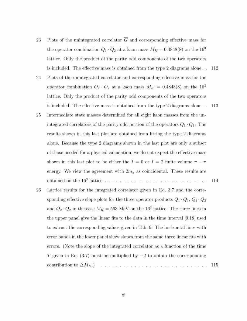
26 Lattice results for the integrated correlator given in Eq. 3.7 and the corre-
sponding effective slope plots for the three operator products Q1 ·Q1, Q1 ·Q2
and Q2 ·Q2 in the case MK = 563 MeV on the 163 lattice. The three lines in
the upper panel give the linear fits to the data in the time interval [9,18] used
to extract the corresponding values given in Tab. 9. The horizontal lines with
error bands in the lower panel show slopes from the same three linear fits with
errors. (Note the slope of the integrated correlator as a function of the time
T given in Eq. (3.7) must be multiplied by −2 to obtain the corresponding
contribution to ∆MK .) . . . . . . . . . . . . . . . . . . . . . . . . . . . . . 115
xi

27 Lattice results for the integrated correlator given in Eq. 3.7 and the corre-
sponding effective slope plots for the three operator products Q1 ·Q1, Q1 ·Q2
and Q2 ·Q2 in the case MK = 707 MeV on the 163 lattice. The three lines in
the upper panel give the linear fits to the data in the time interval [9,18] used
to extract the corresponding values given in Tab. 9. The horizontal lines with
error bands in the lower panel show slopes from the same three linear fits with
errors. (Note the slope of the integrated correlator as a function of the time
T given in Eq. (3.7) must be multiplied by −2 to obtain the corresponding
contribution to ∆MK .) . . . . . . . . . . . . . . . . . . . . . . . . . . . . . 116
28 Lattice results for the integrated correlator given in Eq. 3.7 and the corre-
sponding effective slope plots for the three operator products Q1 ·Q1, Q1 ·Q2
and Q2 ·Q2 in the case MK = 775 MeV on the 163 lattice. The three lines in
the upper panel give the linear fits to the data in the time interval [9,18] used
to extract the corresponding values given in Tab. 9. The horizontal lines with
error bands in the lower panel show slopes from the same three linear fits with
errors. (Note the slope of the integrated correlator as a function of the time
T given in Eq. (3.7) must be multiplied by −2 to obtain the corresponding
contribution to ∆MK .) . . . . . . . . . . . . . . . . . . . . . . . . . . . . . 117
xii

29 Lattice results for the integrated correlator given in Eq. 3.7 and the corre-
sponding effective slope plots for the three operator products Q1 ·Q1, Q1 ·Q2
and Q2 ·Q2 in the case MK = 834 MeV on the 163 lattice. The three lines in
the upper panel give the linear fits to the data in the time interval [9,18] used
to extract the corresponding values given in Tab. 9. The horizontal lines with
error bands in the lower panel show slopes from the same three linear fits with
errors. (Note the slope of the integrated correlator as a function of the time
T given in Eq. (3.7) must be multiplied by −2 to obtain the corresponding
contribution to ∆MK .) . . . . . . . . . . . . . . . . . . . . . . . . . . . . . 118
30 Lattice results for the integrated correlator given in Eq. 3.7 and the corre-
sponding effective slope plots for the three operator products Q1 ·Q1, Q1 ·Q2
and Q2 ·Q2 in the case MK = 918 MeV on the 163 lattice. The three lines in
the upper panel give the linear fits to the data in the time interval [9,18] used
to extract the corresponding values given in Tab. 9. The horizontal lines with
error bands in the lower panel show slopes from the same three linear fits with
errors. (Note the slope of the integrated correlator as a function of the time
T given in Eq. (3.7) must be multiplied by −2 to obtain the corresponding
contribution to ∆MK .) . . . . . . . . . . . . . . . . . . . . . . . . . . . . . 119
xiii
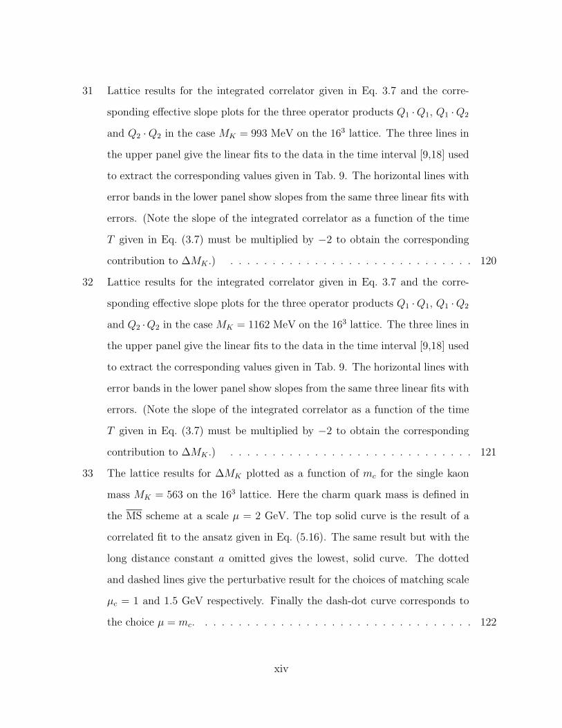
31 Lattice results for the integrated correlator given in Eq. 3.7 and the corre-
sponding effective slope plots for the three operator products Q1 ·Q1, Q1 ·Q2
and Q2 ·Q2 in the case MK = 993 MeV on the 163 lattice. The three lines in
the upper panel give the linear fits to the data in the time interval [9,18] used
to extract the corresponding values given in Tab. 9. The horizontal lines with
error bands in the lower panel show slopes from the same three linear fits with
errors. (Note the slope of the integrated correlator as a function of the time
T given in Eq. (3.7) must be multiplied by −2 to obtain the corresponding
contribution to ∆MK .) . . . . . . . . . . . . . . . . . . . . . . . . . . . . . 120
32 Lattice results for the integrated correlator given in Eq. 3.7 and the corre-
sponding effective slope plots for the three operator products Q1 ·Q1, Q1 ·Q2
and Q2 ·Q2 in the case MK = 1162 MeV on the 163 lattice. The three lines in
the upper panel give the linear fits to the data in the time interval [9,18] used
to extract the corresponding values given in Tab. 9. The horizontal lines with
error bands in the lower panel show slopes from the same three linear fits with
errors. (Note the slope of the integrated correlator as a function of the time
T given in Eq. (3.7) must be multiplied by −2 to obtain the corresponding
contribution to ∆MK .) . . . . . . . . . . . . . . . . . . . . . . . . . . . . . 121
33 The lattice results for ∆MK plotted as a function of mc for the single kaon
mass MK = 563 on the 163 lattice. Here the charm quark mass is defined in
the MS scheme at a scale µ = 2 GeV. The top solid curve is the result of a
correlated fit to the ansatz given in Eq. (5.16). The same result but with the
long distance constant a omitted gives the lowest, solid curve. The dotted
and dashed lines give the perturbative result for the choices of matching scale
µc = 1 and 1.5 GeV respectively. Finally the dash-dot curve corresponds to
the choice µ = mc. . . . . . . . . . . . . . . . . . . . . . . . . . . . . . . . . 122
xiv
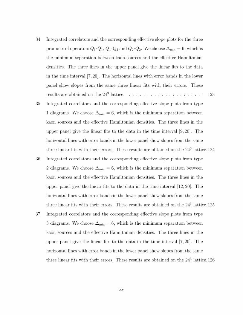
34 Integrated correlators and the corresponding effective slope plots for the three
products of operators Q1·Q1, Q1·Q2 and Q2·Q2. We choose ∆min = 6, which is
the minimum separation between kaon sources and the effective Hamiltonian
densities. The three lines in the upper panel give the linear fits to the data
in the time interval [7, 20]. The horizontal lines with error bands in the lower
panel show slopes from the same three linear fits with their errors. These
results are obtained on the 243 lattice. . . . . . . . . . . . . . . . . . . . . . 123
35 Integrated correlators and the corresponding effective slope plots from type
1 diagrams. We choose ∆min = 6, which is the minimum separation between
kaon sources and the effective Hamiltonian densities. The three lines in the
upper panel give the linear fits to the data in the time interval [9, 20]. The
horizontal lines with error bands in the lower panel show slopes from the same
three linear fits with their errors. These results are obtained on the 243 lattice.124
36 Integrated correlators and the corresponding effective slope plots from type
2 diagrams. We choose ∆min = 6, which is the minimum separation between
kaon sources and the effective Hamiltonian densities. The three lines in the
upper panel give the linear fits to the data in the time interval [12, 20]. The
horizontal lines with error bands in the lower panel show slopes from the same
three linear fits with their errors. These results are obtained on the 243 lattice.125
37 Integrated correlators and the corresponding effective slope plots from type
3 diagrams. We choose ∆min = 6, which is the minimum separation between
kaon sources and the effective Hamiltonian densities. The three lines in the
upper panel give the linear fits to the data in the time interval [7, 20]. The
horizontal lines with error bands in the lower panel show slopes from the same
three linear fits with their errors. These results are obtained on the 243 lattice.126
xv
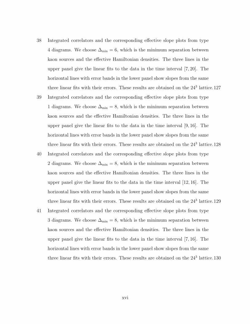
38 Integrated correlators and the corresponding effective slope plots from type
4 diagrams. We choose ∆min = 6, which is the minimum separation between
kaon sources and the effective Hamiltonian densities. The three lines in the
upper panel give the linear fits to the data in the time interval [7, 20]. The
horizontal lines with error bands in the lower panel show slopes from the same
three linear fits with their errors. These results are obtained on the 243 lattice.127
39 Integrated correlators and the corresponding effective slope plots from type
1 diagrams. We choose ∆min = 8, which is the minimum separation between
kaon sources and the effective Hamiltonian densities. The three lines in the
upper panel give the linear fits to the data in the time interval [9, 16]. The
horizontal lines with error bands in the lower panel show slopes from the same
three linear fits with their errors. These results are obtained on the 243 lattice.128
40 Integrated correlators and the corresponding effective slope plots from type
2 diagrams. We choose ∆min = 8, which is the minimum separation between
kaon sources and the effective Hamiltonian densities. The three lines in the
upper panel give the linear fits to the data in the time interval [12, 16]. The
horizontal lines with error bands in the lower panel show slopes from the same
three linear fits with their errors. These results are obtained on the 243 lattice.129
41 Integrated correlators and the corresponding effective slope plots from type
3 diagrams. We choose ∆min = 8, which is the minimum separation between
kaon sources and the effective Hamiltonian densities. The three lines in the
upper panel give the linear fits to the data in the time interval [7, 16]. The
horizontal lines with error bands in the lower panel show slopes from the same
three linear fits with their errors. These results are obtained on the 243 lattice.130
xvi
42 Integrated correlators and the corresponding effective slope plots from type
4 diagrams. We choose ∆min = 8, which is the minimum separation between
kaon sources and the effective Hamiltonian densities. The three lines in the
upper panel give the linear fits to the data in the time interval [7, 16]. The
horizontal lines with error bands in the lower panel show slopes from the same
three linear fits with their errors. These results are obtained on the 243 lattice.131
43 Integrated correlators for the operator products (Qi · sd) and (sd · sd). We
choose ∆min = 6, which is the minimum separation between the kaon sources
and the weak Hamiltonians. These results are obtained from the 243 lattice. 132
44 Integrated correlators and the corresponding effective slope plots for cp = 1
and cs = −1. cs and cp are defined in Eq.6.1. We choose ∆min = 6, which is
the minimum separation between kaon sources and the effective Hamiltonian
densities. The three lines in the upper panel give the linear fits to the data
in the time interval [7, 20]. The horizontal lines with error bands in the lower
panel show slopes from the same three linear fits with their errors. These
results are obtained on the 243 lattice. . . . . . . . . . . . . . . . . . . . . . 133
45 Integrated correlators and the corresponding effective slope plots for cp = 1
and cs = 1. cs and cp are defined in Eq.6.1. We choose ∆min = 6, which is
the minimum separation between kaon sources and the effective Hamiltonian
densities. The three lines in the upper panel give the linear fits to the data
in the time interval [7, 20]. The horizontal lines with error bands in the lower
panel show slopes from the same three linear fits with their errors. These
results are obtained on the 243 lattice. . . . . . . . . . . . . . . . . . . . . . 134
xvii
46 Integrated correlators and the corresponding effective slope plots for cp = 1
and cs = −1.14(26). cs and cp are defined in Eq.6.1. This value of cs will
eliminate the η intermediate state. We choose ∆min = 6, which is the minimum
separation between kaon sources and the effective Hamiltonian densities. The
three lines in the upper panel give the linear fits to the data in the time interval
[7, 20]. The horizontal lines with error bands in the lower panel show slopes
from the same three linear fits with their errors. These results are obtained
on the 243 lattice. . . . . . . . . . . . . . . . . . . . . . . . . . . . . . . . . . 135
47 Mass difference for different choice of cs while fixing cp = 1. We choose
∆min = 6, which is the minimum separation between the kaon sources and the
weak Hamiltonians. The minimal fitting time Tmin is 7. Results are given for
different operator products and for their sum. These results are obtained on
the 243 lattice. . . . . . . . . . . . . . . . . . . . . . . . . . . . . . . . . . . 136
48 Integrated correlator for cp = 0 and cs = 0. We give the results for both
∆min = 6 and ∆min = 10. ∆min is the minimum separation between the kaon
sources and the weak Hamiltonians. All the standard exponentially increasing
terms have been removed. The straight lines give the linear fits to the data
in the time interval [7,12]. These results are obtained on the 243 lattice. . . . 137
49 Mass difference for different choice of cp while fixing cs = 0. We choose
∆min = 10, which is the minimum separation between the kaon sources and
the weak Hamiltonians. The minimal fitting time Tmin is 7. Results are given
for different operator products and for their sum. These results are obtained
on the 243 lattice. . . . . . . . . . . . . . . . . . . . . . . . . . . . . . . . . . 138
xviii
50 fqq as a function of quark mass mq on the 243 lattice. The quantity fqq is the
product of the pseudoscalar decay constant and the normalizaiton factor of
the gauge fixed wall source. (The author thanks Ziyuan Bai for providing this
figure.) . . . . . . . . . . . . . . . . . . . . . . . . . . . . . . . . . . . . . . . 139
xix
ACKNOWLEDGMENTS
I would like to thank my advisor Prof. Norman Christ very much for his guidance,
suggestions, encouragements, and help during my research at Columbia University. I really
enjoyed the weekly discussions, and learned a lot.
I am grateful to Prof. Robert Mawhinney for all the insightful discussions, help on the
machines and other suggestions. I would also like to thank Prof. Chris Sachrajda, Armarjit
Soni, Taku Izubuchi for instructions and help on all kinds of problems. I greatly appreciate
Ziyuan Bai’s work on checking part of my calculation.
I enjoyed working and benefited a lot from all my colleagues: Tom Blum, Luchang Jin,
Chris Kelly, Christoph Lehner, Qi Liu, Zhongjie Lin, Greg McGlynn, Hantao Yin, Daiqian
Zhang, I would like to thank all of them for the discussions and help.
xx

Chapter 1
Introduction
The standard model of particle physics is a theory using quantum filed theory to describe the
dynamics of subatomic particles. The current formulation of the standard model was finalized
in the 1970s. Then the discoveries of the W± and Z boson, the top quark, the tau neutrino
and finally the Higgs boson all confirm the correctness of the standard model. Because the
standard model can explain a wide variety of experimental results, it is considered to be a
theory of almost everything.
There are three fundamental interactions in the standard model: electromagnetic (EM),
weak and strong interactions. We believe that we have fully understood the EM interaction
with the theory of quantum electrodynamics (QED), which has withstood some of the most
stringent experimental tests in the history of physics. The excellent agreement between
the experimental and theoretical values of the anomalous magnetic dipole moment of the
electron is considered to be one of the most significant triumphs of physics during the last
century.
The strong interaction is described by quantum chromodynamics (QCD) in the standard
model. Although QCD is widely believed to be well understood, its analytic treatment at low
energy is extremely difficult if not entirely impossible. Perturbation theory calculation fail
at an energy scale of ΛQCD, because the coupling constant becomes equal to or larger than
1
2
O(1). Other analytical methods such as chiral perturbation theory are also unsatisfactory.
These methods are usually not from first principles and require input parameters other than
the parameters of the standard model. More importantly, these methods are usually not
able to give precise enough predictions for low energy QCD effects.
The weak interaction is the least understood part of the standard model and is considered
to be the place where new physics may be discovered. However, various tests of the weak
interaction have been done and no significant discrepancy from the standard model has been
found. Among the ongoing lattice calculations, the unitarity of the Cabibbo-Kobayashi-
Maskawa (CKM) matrix and both the direct and indirect CP violation parameters may be
the most interesting tests. These calculations are usually quite difficult. The weak interaction
itself can be treated precisely with perturbation theory. However, many interesting weak
interaction processes involve mesons and baryons. A full calculation of such process requires
inputs from non-pertrubative QCD calculation.
Lattice QCD is the only known method to provide first-principal calculation of non-
perturbative QCD effects in electroweak processes. Due to both theoretical and practical
reasons, we usually don’t simulate weak interaction processes directly on lattice. The stanard
approach is to split the energy scale into high (> µ) and low (< µ). We start from the full
standard model and integrate out the W± and Z bosons. The weak interaction process will
be described by an effective Hamiltonian. We use perturbation theory to run the Wilson
coefficients from the W meson mass scale to a lower scale µ. The physics above the scale
µ is encoded in the Wilson coefficients of the effective Hamiltonian. The low-energy part of
the weak matrix element is a pure non-perturbative QCD problem and can be solved using
lattice QCD techniques.
At the early stage of lattice QCD, due to the limitation of computing resources, most
of the lattice calculations were done at unphysical kinematics without dynamical fermions
(quenched approximation). During the last few decades, the computing power of supercom-
3
puters has been improved by a few order of magnitudes. The development of the lattice
algorithms has boosted the efficiency tremendously. Simulations at physical kinematics with
full dynamical fermions became possible in recent years. Actually, the measurement of the
standard quantities such as fK , fπ have reached sub-percent level precision. At such pre-
cision, isospin breaking effects and QED corrections become important. Many efforts and
computing resources are invested to further improve the precision of these measurements.
However, we should be aware that there are some other more interesting quantities that can
be calculated with lattice QCD. Among many such quantities, the KL −KS mass difference
is one of the most interesting ones.
The kaon mass difference ∆MK with a value of 3.483(6) × 10−12 MeV [4] plays a very
important role in the history of particle physics. It led to the prediction of charm quark fifty
years ago [5, 6, 7]. This extremely small mass difference is believed to arise from K0-K0
mixing via second-order weak interaction. However, because it arises from an amplitude in
which strangeness changes by two units, this is a promising quantity to reveal new phenomena
which lie outside the standard model. A closely related quantity is the indirect CP violation
parameter ǫK , which arises from the same process. The experimental value of ∆MK and ǫK
are both known very accurately, making the precise calculation of ∆MK and ǫK an important
challenge.
In perturbation theory calculations, the standard model contribution to ∆MK is sepa-
rately into short distance and long distance parts. The short distance part receives most
contributions from momenta on the order of the charm quark mass. As pointed out in the
recent next-to-next-to-leading-order (NNLO) calculation [8], the NNLO terms are as large
as 36% of the leading order (LO) and next-to-leading order (NLO) terms, raising doubts
about the convergence of the QCD perturbation series at this energy scale. The long dis-
tance part of ∆MK can receive contributions from distance as large as 1/mπ. So far there
is no result with controlled uncertainty available since this is highly non-perturbative. How-
4
ever, an estimation given by Donoghue et. al. [9] suggest that there can be sizable long
distance contributions. The calculation of ǫK is under much better control and the largest
contribution involves momenta on the scale of top quark mass. However, the same NNLO
difficulties in the predicting the charm quark contribution to ǫK enters at the 8% level. In
addition, the long distance part of ǫK , which is estimated to be 3.6% by Buras et al. [10],
also becomes increasing interesting and non-perturbative methods are required for a more
reliable calculation.
It is customary when discussing the KL-KS mass difference to follow the convention of
referring to distance scales at or below 1/mc as short distance and those larger than 1/mc as
long distance. We will follow this convention here. However, since the perturbation theory
calculation of ∆MK at the charm quark mass scale converges badly, the inverse charm quark
mass represents a somewhat large distance to act as a boundary between the short and long
distance regions. Non-perturbative methods are needed for the proper treatment of short
distance contributions at the charm quark mass scale and that it may be better to adopt a
shorter distance demarcation between short and long distances in the future.
Here we propose a method to computeKL−KS mass difference including the long distance
effects on a Euclidean lattice [11]. We devise an Euclidean-space amplitude which can be
evaluated in lattice QCD and which contains the second-order mass difference of interest.
As explained in the following chapters, we perform a second-order integration of the product
of two first-order weak Hamiltonians in a given space-time volume. The integration sums
the contribution to the mass difference from all possible intermediate states.
A generalization of the Lellouch-Luscher method [12] is used to correct potentially large
finite-volume effects coming from the two-pion state which can be degenerate with the kaon
and the associated principal part appearing in the infinite volume integral over intermediate
states [11]. This is an important part of this proposal. However, in the kinematic region
studied in this paper, we are unable to resolve the two-pion intermediate state signal from
5
statistical fluctuations, so this last piece cannot be studied numerically. We therefore only
give a theoretical discussion in this thesis.
Our first preliminary work is performed on a 2+1 flavor, domain wall fermion (DWF),
163 × 32× 16 lattice ensemble with a 421 MeV pion. We drop the double penguin diagrams
and the disconnected diagrams in this first exploratory calculation. Although this is a non-
unitary calculation at unphysical kinematics, the main purpose of this work is to show that
the second order weak process can be evaluated using lattice methods. Then a full calculation
is performed on a 243×64×16 ensemble with a 330 Mev pion. Although the inclusion of the
disconnected diagrams increased the noise substantially, we are able to get a good statistical
error with more sophisticated measuring techniques.
This work is organized as follows. In Chapter 2, we review the K0 −K0mixing in the
standard model and give a brief summary of the perturbation theory calculation. Chapter
3 summarizes all the building blocks of a lattice QCD calculation of the KL − KS mass
difference; In Chapter 4, we discuss the lattice measurement methods used in our calculation;
Chapter 5 and 6 give the results from a 163 × 32× 16 lattice ensemble and a 243 × 64× 16
lattice ensemble respectively. In Chapter 7, we discuss our results and future prospects.

Chapter 2
Kaon Mixing in the Standard Model
In this chapter, we will discuss the neutral kaon mixing in the Standard Model. We start from
basic quantum mechanics and give the standard formalism for the KL −KS mass difference
∆MK and the indirect CP violation parameter ǫK . After that we explain the perturbation
theory calculation of K0 − K0mixing in the Standard Model. Then we summarized the
NNLO results and discuss the limitations of these calculations.
2.1 K0 −K0Mixing
One of the most interesting features of the neutral K mesons is the mixing of the K0 and K0.
The K0 meson with strangeness +1 and the K0meson with strangeness −1 are eigenstates
of the strong interaction Hamiltonian. They are antiparticle of each other and have identical
mass. However, the weak interactions do not conserve strangeness and cause the mixing of
the K0 and K0. The strangeness of these two mesons are differ by two. Hence the K0 −K
0
mixing is a second order weak process and the amplitude of this process are extremely small.
The K0 and K0state are charge conjugates of each other
C|K0〉 = |K0〉, C|K0〉 = |K0〉. (2.1)
6
7
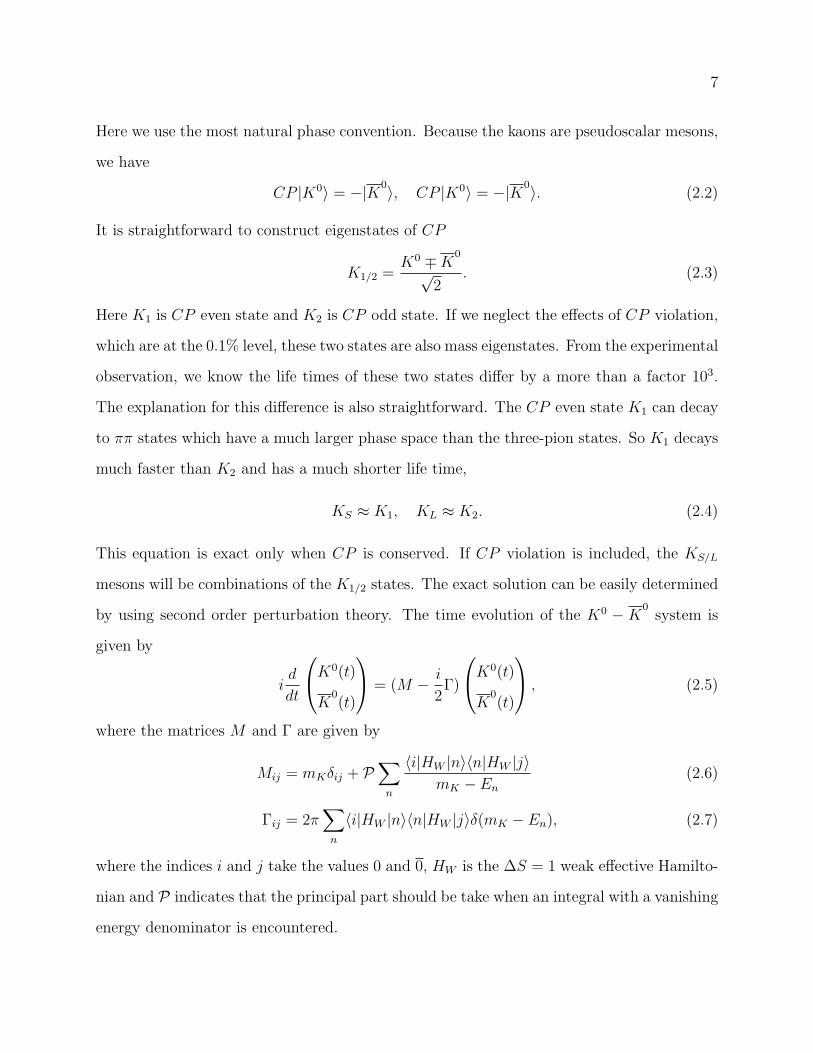
Here we use the most natural phase convention. Because the kaons are pseudoscalar mesons,
we have
CP |K0〉 = −|K0〉, CP |K0〉 = −|K0〉. (2.2)
It is straightforward to construct eigenstates of CP
K1/2 =K0 ∓K
0
√2
. (2.3)
Here K1 is CP even state and K2 is CP odd state. If we neglect the effects of CP violation,
which are at the 0.1% level, these two states are also mass eigenstates. From the experimental
observation, we know the life times of these two states differ by a more than a factor 103.
The explanation for this difference is also straightforward. The CP even state K1 can decay
to ππ states which have a much larger phase space than the three-pion states. So K1 decays
much faster than K2 and has a much shorter life time,
KS ≈ K1, KL ≈ K2. (2.4)
This equation is exact only when CP is conserved. If CP violation is included, the KS/L
mesons will be combinations of the K1/2 states. The exact solution can be easily determined
by using second order perturbation theory. The time evolution of the K0 − K0system is
given by
id
dt
K0(t)
K0(t)
= (M − i
2Γ)
K0(t)
K0(t)
, (2.5)
where the matrices M and Γ are given by
Mij = mKδij + P∑
n
〈i|HW |n〉〈n|HW |j〉mK − En
(2.6)
Γij = 2π∑
n
〈i|HW |n〉〈n|HW |j〉δ(mK − En), (2.7)
where the indices i and j take the values 0 and 0, HW is the ∆S = 1 weak effective Hamilto-
nian and P indicates that the principal part should be take when an integral with a vanishing
energy denominator is encountered.
8
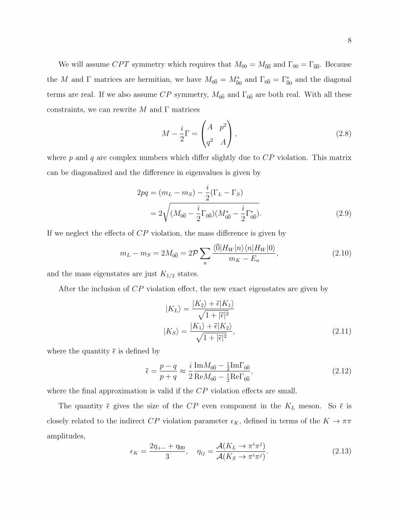
We will assume CPT symmetry which requires that M00 = M00 and Γ00 = Γ00. Because
the M and Γ matrices are hermitian, we have M00 = M∗00
and Γ00 = Γ∗00
and the diagonal
terms are real. If we also assume CP symmetry, M00 and Γ00 are both real. With all these
constraints, we can rewrite M and Γ matrices
M − i
2Γ =
A p2
q2 A
, (2.8)
where p and q are complex numbers which differ slightly due to CP violation. This matrix
can be diagonalized and the difference in eigenvalues is given by
2pq = (mL −mS)−i
2(ΓL − ΓS)
= 2
√(M00 −
i
2Γ00)(M
∗00− i
2Γ∗00). (2.9)
If we neglect the effects of CP violation, the mass difference is given by
mL −mS = 2M00 = 2P∑
n
〈0|HW |n〉〈n|HW |0〉mK − En
, (2.10)
and the mass eigenstates are just K1/2 states.
After the inclusion of CP violation effect, the new exact eigenstates are given by
|KL〉 =|K2〉+ ǫ|K1〉√
1 + |ǫ|2
|KS〉 =|K1〉+ ǫ|K2〉√
1 + |ǫ|2, (2.11)
where the quantity ǫ is defined by
ǫ =p− q
p+ q≈ i
2
ImM00 − i2ImΓ00
ReM00 − i2ReΓ00
, (2.12)
where the final approximation is valid if the CP violation effects are small.
The quantity ǫ gives the size of the CP even component in the KL meson. So ǫ is
closely related to the indirect CP violation parameter ǫK , defined in terms of the K → ππ
amplitudes,
ǫK =2η+− + η00
3, ηij =
A(KL → πiπj)
A(KS → πiπj). (2.13)

9
Following the usual convention, we introduce the definite isospin amplitudes A0 and A2,
AIeδI = A(K → ππ(I)), (2.14)
where δI is the strong phase from the π-π interaction. The π+π− and π0π0 states are related
to the states with definite isospin by
|π+π−〉 = 1√3
(|ππ(I = 2)〉+
√2|ππ(I = 0)〉
)
|π0π0〉 = 1√3
(−√2|ππ(I = 2)〉+ |ππ(I = 0)〉
). (2.15)
Substituting Eq. 2.15 and 2.11 into Eq. 2.13 and dropping all the (ReA2/ReA0)2 term gives
ǫK = ǫ+ iξ, (2.16)
where ξ is the weak phase of the K0 → (ππ)I=0 amplitude,
ξ =ImA0
ReA0
(2.17)
In order to evaluate ǫK more conveniently, we can simplify the expression by defining the
superweak phase
φǫ = arctan
(−2ReM00
Γ00
). (2.18)
We can use the observation that the |(ππ)I=0〉 states dominate the sum in Eq. 2.7, which
implies
ImΓ00
ReΓ00
≈ −2ImA0
ReA0
= −2ξ. (2.19)
Combining all these together we arrive
ǫK = eiφǫsinφǫ
(ImM00
∆mK
+ ξ
)(2.20)
The experimental value for φǫ is close to 45◦. The ξ term contributes to ǫK at the few percent
level.

10
2.2 Perturbation Theory Calculation for ∆MK
In the standard model, the largest contribution to K0 − K0mixing comes from the box
diagrams as shown in Fig. 1. We should notice that there are also contributions from double
penguin diagrams and disconnected diagrams. These diagrams will start to contribute if
we include higher order QCD effects. It is customary when discussing K0 − K0mixing
to separate the results into the top contribution, the charm contribution and the charm-
top contribution. These different contributions come from different choices of two quark
propagators in the loop inside the box diagram.
To evaluate the mixing process, we can construct a low energy effective filed theory and
encode the short distance physics into the Wilson coefficients in the effective theory. First the
W bosons and the top quarks are integrated out. The top component is then described by a
local ∆S = 2 effective Hamiltonian. The charm component is described by bilocal operators,
i .e., the products of two ∆S = 1 effective Hamiltonians. The charm-top component is
more complicated due to the presence of penguin operators. The effective Hamiltonian of
the charm-top component contains both bilocal operators and local counterterms. Fig. 2
gives some examples of the contributions from the bilocal operators. Next, these effective
Hamiltonians are renormalized at the charm quark scale. Finally, we integrate out the charm
quark and renormalize the effective Hamiltonian at a low scale µ. The effective low energy
Hamiltonian can be written as:
H∆S=2eff (µ) =
G2F
16π2M2
W
(λ2cηccS0(xc) + λ2
tλ2tηttS0(xt) + 2λcλtηctS0(xc, xt)
)b(µ)Q(µ) + h.c.
(2.21)
where λi = V ∗isVid and xi = m2
i /m2W . The basic electroweak loop contributions without QCD
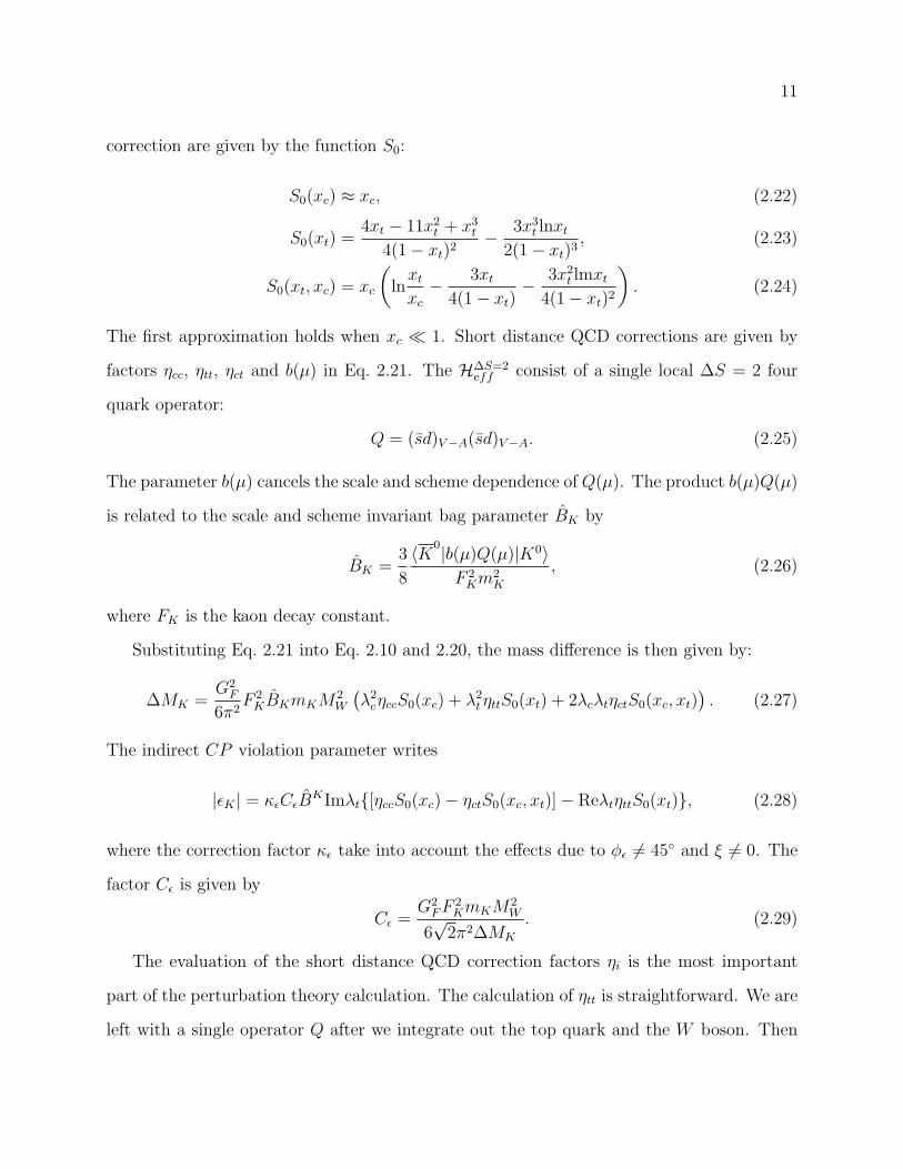
11
correction are given by the function S0:
S0(xc) ≈ xc, (2.22)
S0(xt) =4xt − 11x2
t + x3t
4(1− xt)2− 3x3
t lnxt
2(1− xt)3, (2.23)
S0(xt, xc) = xc
(lnxt
xc
− 3xt
4(1− xt)− 3x2
t lmxt
4(1− xt)2
). (2.24)
The first approximation holds when xc ≪ 1. Short distance QCD corrections are given by
factors ηcc, ηtt, ηct and b(µ) in Eq. 2.21. The H∆S=2eff consist of a single local ∆S = 2 four
quark operator:
Q = (sd)V−A(sd)V−A. (2.25)
The parameter b(µ) cancels the scale and scheme dependence of Q(µ). The product b(µ)Q(µ)
is related to the scale and scheme invariant bag parameter BK by
BK =3
8
〈K0|b(µ)Q(µ)|K0〉F 2Km
2K
, (2.26)
where FK is the kaon decay constant.
Substituting Eq. 2.21 into Eq. 2.10 and 2.20, the mass difference is then given by:
∆MK =G2
F
6π2F 2KBKmKM
2W
(λ2cηccS0(xc) + λ2
tηttS0(xt) + 2λcλtηctS0(xc, xt)). (2.27)
The indirect CP violation parameter writes
|ǫK | = κǫCǫBKImλt{[ηccS0(xc)− ηctS0(xc, xt)]− ReλtηttS0(xt)}, (2.28)
where the correction factor κǫ take into account the effects due to φǫ 6= 45◦ and ξ 6= 0. The
factor Cǫ is given by
Cǫ =G2
FF2KmKM
2W
6√2π2∆MK
. (2.29)
The evaluation of the short distance QCD correction factors ηi is the most important
part of the perturbation theory calculation. The calculation of ηtt is straightforward. We are
left with a single operator Q after we integrate out the top quark and the W boson. Then

12
we renormalize this operator at a low scale µ and we will obtain ηtt. The calculation of ηcc
is more complicated. We need to deal with the product of two ∆S = 1 operators. At the
charm quark threshold, we need to match this bi-local operator with the local operator Q.
Top-charm contribution ηct is the most difficult one due to the presence of penguin operators.
The top contribution is known at NLO:
ηtt = 0.5765(65) (2.30)
The result is very precise since the perturbation theory should work well at the scale of top
quark mass. Higher order calculation for ηtt is unnecessary. The charm-top contribution has
been evaluated to NNLO:
ηct = 0.496(47). (2.31)
∆MK receives most of the contribution from the momenta at the scale of charm quark mass.
Unfortunately, the factor ηcc has the largest uncertainty among all the three factors. The
reason is the slow convergence of the perturbation series at the scale of charm quark mass.
We can compare the NLO result with the NNLO result. At NLO,
ηNLOcc = 1.38± 0.52µc
± 0.07µW± 0.02αs
. (2.32)
We can see that the largest uncertainty comes from the dependence on the charm threshold
µc. If perturbation theory works well, we would expect a smaller dependence on µc at NNLO.
However, the size of uncertainty is similar in the NNLO result:
ηNNLOcc = 1.86± 0.53µc
± 0.07µW± 0.06αs
. (2.33)
Also, there is a large positive shift of 36% in the central value. The NNLO result suggest
that the perturbation series converges very badly. Brod et.al. suggest we can use the size of
NNLO correction as the theoretical uncertainty, which leads to a 36% total uncertainty:
ηcc = 1.87± 0.76. (2.34)
13
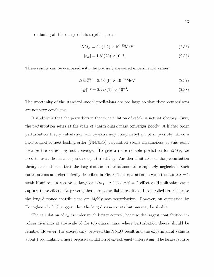
Combining all these ingredients together gives:
∆MK = 3.1(1.2)× 10−12MeV (2.35)
|ǫK | = 1.81(28)× 10−3. (2.36)
These results can be compared with the precisely measured experimental values:
∆M expK = 3.483(6)× 10−12MeV (2.37)
|ǫK |exp = 2.228(11)× 10−3. (2.38)
The uncetanity of the standard model predictions are too large so that these comparisons
are not very conclusive.
It is obvious that the perturbation theory calculation of ∆MK is not satisfactory. First,
the perturbation series at the scale of charm quark mass converges poorly. A higher order
perturbation theory calculation will be extremely complicated if not impossible. Also, a
next-to-next-to-next-leading-order (NNNLO) calculation seems meaningless at this point
because the series may not converge. To give a more reliable prediction for ∆MK , we
need to treat the charm quark non-perturbatively. Another limitation of the perturbation
theory calculation is that the long distance contributions are completely neglected. Such
contributions are schematically described in Fig. 3. The separation between the two ∆S = 1
weak Hamiltonian can be as large as 1/mπ. A local ∆S = 2 effective Hamiltonian can’t
capture these effects. At present, there are no available results with controlled error because
the long distance contributions are highly non-perturbative. However, an estimation by
Donoghue et .al . [9] suggest that the long distance contributions may be sizable.
The calculation of ǫK is under much better control, because the largest contribution in-
volves momenta at the scale of the top quark mass, where perturbation theory should be
reliable. However, the discrepancy between the NNLO result and the experimental value is
about 1.5σ, making a more precise calculation of ǫK extremely interesting. The largest source
14
of uncertainty is the CKM matrix element Vcb. The second largest one is ηcc, which con-
tribute about 8% uncertainty to ǫK . A more precise calculation will require non-perturbative
method. In addition the long distance contribution to ǫK is estimated to be -3.6% by Buras
et al. [10], again suggesting the need for a reliable, non-perturbative method.
Chapter 3
K0-K mixing from Lattice QCD
In this chapter we will discuss the details about evaluatingK0-K0mixing process with lattice
QCD. In Section 3.1, we discuss the second order weak amplitude and the method to extract
∆MK from such amplitude. In Section 3.2, we give all the Wick contractions in the lattice
calculation. Section 3.3 will discuss the calculation of the Wilson coefficients. In Section 3.4,
we will discuss the renormalization of the ∆S = 1 four-quark operators. In Section 3.5,
we give a theoretical discussion on the subtraction of short distance effects on lattice. In
Section 3.6, we discuss the finite volume effects in the ∆MK calculation.
3.1 Second Order Weak Amplitude
Lattice QCD has been used to calculate K0-K0mixing for a long time. However, all the
previous calculation use a local ∆S = 2 effective Hamiltonian defined in Eq. 3.1. The purpose
of these calculations is to evaluate the BK parameter. As we have discussed at the end of
Section. 2.2, these calculations suffer from non-perturbative effects at the scale of charm
quark mass and uncontrolled long distance effects. In order to resolve these difficulties,
we need to evaluate the second order weak process directly using lattice QCD. The typical
inverse lattice spacing is a few GeVs. So we can’t directly put the W boson and the top
15
16
quark on the lattice. These heavy degree of freedoms are integrated out, leaving us with
a product of two ∆S = 1 effective weak Hamiltonians. The effective Hamiltonian in this
process is given by:
H∆S=1W =
GF√2
∑
q,q′=u,c
VqdV∗q′s(C1Q
qq′
1 + C2Qqq′
2 ) (3.1)
where q and q′ are each on of the u and c quarks, Vqd and Vq′s are the CKM matrxi elements,
C1 and C2 are the Wilson coefficients and Qi are the current-current operators, which are
defined as:
Qqq′1 = (siq
′j)V−A(qjdi)V−A (3.2)
Qqq′2 = (siq
′i)V−A(qjdj)V−A , (3.3)
where i, j are color indices and the spinor indices are contracted within each pair of brackets.
In order to evaluate the K0-K0process, the most natural thoughts will be calculating
the four point correlators:
G(tf , t2, t1, ti) = 〈0|T{K
0(tf )HW (t2)HW (t1)K
0(ti)
}〉, (3.4)
where T is the usual time ordering operator. Here the initial K0 states is generated by kaon
source K0(ti) at time ti and the final K
0state is destroyed by the anti-kaon sink K
0(tf ).
The two ∆S = 1 effective Hamiltonian acts at the time t1 and t2. Assuming that the time
separations tf − tk and tk − ti for k = 1 and 2 are sufficiently large that kaon interpolating
operator will project onto theK0 andK0initial and final states and after inserting a complete
set of energy eigenstates, we find:
G(tf , t2, t1, ti) = N2Ke
−MK(tf−ti)∑
n
〈K0|HW |n〉〈n|HW |K0〉e−(En−MK)|t2−t1|, (3.5)
where Nk is the normalization factor for the kaon interpolation operator and |n〉 are the
eigenstates of the QCD Hamiltonian. If we fix the time ti and tf , then this correlator de-
pends only on the time separation between the two Hamiltonians |t2 − t1|. We will refer to
17
G(tf , t2, t1, ti) as the unintegrated correlator. The unintegrated correlator receives contribu-
tions from all possible intermediate states. The terms in this sum over intermediate states
show exponentially decreasing or increasing behavior with increasing separation |t2 − t1|
depending on whether En lies above or below MK .
In order to get a lattice approximation to the mass difference defined in Eq. 2.10, we can
start from the unintegrated correlator and integrate it over a time interval. There are a few
possible choices of the integration time interval. We will discuss our choice of method first
and discuss the alternatives later. We choose an integration time interval [ta, tb] and obtain:
A =1
2
tb∑
t2=ta
tb∑
t1=ta
〈0|T{K0(tf )HW (t2)HW (t1)K0(ti)
}|0〉, (3.6)
where ta − ti and tf − tb should be sufficiently large that the kaon interpolating operators
to project onto kaon states. We will refer to this correlator as the integrated correlator.
The integrated correlator is represented schematically in Fig. 4. After inserting a sum over
intermediate states and summing explicitly over t1 and t2 in the interval [ta, tb] one obtains:
A =N2Ke
−MK(tf−ti)
{∑
n 6=n0
〈K0|HW |n〉〈n|HW |K0〉MK − En
(−T +
e(MK−En)T − 1
MK − En
)
+1
2〈K0|HW |n0〉〈n0|HW |K0〉T 2
}.
(3.7)
Here T = tb − ta + 1 and the sum includes all possible intermediate states except a possible
state |n0〉 which is degenerate with the kaon, En0= MK . Such a state will exist only if the
spatial volume of the lattice is adjusted to some specific value. The contribution from such a
degenerate state appears separately as the final term on the right hand side of this equation.
In order to obtain Eq. 3.7, we neglect all the O((Ena)2) terms.
The coefficient of the term which is proportional to T in Eq. 3.7 gives the finite-volume
approximation to ∆MK up to some normalization factors:
∆MFVK = 2
∑
n 6=n0
〈K0|HW |n〉〈n|HW |K0〉MK − En
. (3.8)
18
The other terms in Eq. 3.7 can be classified into four categories according to their dependence
on T :
i) The term independent of T within the large parentheses. This constant does not affect
our determination of the mass difference from A.
ii) Terms exponentially decreasing as T increases coming from states |n〉 with En > MK .
These terms are negligible for sufficiently large T .
iii) Terms exponentially increasing as T increases coming from states |n〉 with En < MK .
These will be the largest contributions when T is large and must be removed as dis-
cussed in the paragraph below.
iv) The final term proportional to T 2 coming from states degenerate with the kaon. As
discussed below, this term must be identified and removed in order to relate the finite-
and infinite-volume expressions for ∆MK following the method of Ref. [11].
The exponentially growing terms, introduced in item iii) above, pose a significant chal-
lenge. Fortunately, the two leading terms corresponding to the vacuum and single pion states
can be computed separately and removed. The matrix elements 〈π0|HW |K0〉 and 〈0|HW |K0〉
can be obtained from the three-point and two-point correlation functions:
〈0|π0(tπ)HW (tO)K0†(tK)|0〉 = NπNKe
−mπ(tπ−tO)e−mK(tO−tK)〈π0|HW |K0〉 (3.9)
〈0|HW (tO)K0†(tK)|0〉 = NKe
−mK(tO−tK)〈0|HW |K0〉. (3.10)
Here we assume that the time separations tπ − tO and tO − tK are sufficiently large that only
the pion and kaon states contribute. The matrix element can be obtained from the ratio of
the correlation functions in Eqs. 3.9 and 3.10 with the corresponding two-point correlators
of the operators K0 and π0 to remove the tO dependence. This will be discussed in more
details in Section. 4.3. Then we can use these matrix elements to remove the single-pion and
vaccum exponential growing terms in Eq. 3.7.
19
A second approach to remove these two unwanted exponentially growing terms exploits
the lattice Ward identities to add to HW terms proportional to the scalar and pseudo-scalar
densities, sd and sγ5d. The new Hamiltonian is given by:
H ′W = HW + c1sd+ c2sγ
5d. (3.11)
The coefficients c1 and c2 are chosen to eliminate the single-pion and vacuum intermediate
states:
〈π0|HW + c1sd|K0〉 = 0, (3.12)
〈0|HW + c2sγ5d|K0〉 = 0. (3.13)
The coefficient is then given by:
cπ = −〈π0|HW |K0〉〈π0|sd|K0〉 , (3.14)
cvac = − 〈0|HW |K0〉〈0|sγ5d|K0〉 . (3.15)
Since these two densities can be written as the divergence of the vector and axial currents
respectively, they cannot contribute to the mass difference given in 3.8. This approach is
similar to the subtraction in the previous paragraph, but instead of removing only the expo-
nentially growing term in Eq. 3.7, such an addition will remove all single pion and vacuum
contributions from that equation, including their appearance in the sum over intermediate
states |n〉.
A third approach is multi-parameter fitting. We can add these exponential terms into
the fitting ansatz. In principal, we can get the mass difference from a multi-parameter fit.
However, this approach can be very noisy, especially when the exponentially increasing term
is significantly larger than the linear term.
Two-pion states with energies below MK may also exist and, if present, must be explicitly
identified and removed. For the kinematics studies in this thesis, the only π-π state with
20
an energy possibly below MK is the state with two pions at rest. In our calculation on 163
lattice with a 412 MeV pion mass, we study the contribution of this state as the kaon mass
varied. However, we are not able to identify a clear two-pion signal. In our calculation on
243 with a 330 MeV pion mass and a 575 MeV kaon mass, there is no π-π state lighter than
the kaon. Thus we don’t need to worry about it. However, in a future calculation in physical
kinematics, the two pion states will pose a significant challenge. More studies are needed to
solve this problem.
So far all our discussions are based on Eq. 3.6. However, there are alternative choices
for the integrated correlators. For example, a simpler alternative integrates the two weak
operators over the full time interval [ti, tf ] between the kaon source and sink instead of the
the restricted interval [ta, tb] used here:
A′ =1
2
tf∑
t2=ti
tf∑
t1=ti
〈0|T{K0(tf )HW (t2)HW (t1)K0(ti)
}|0〉. (3.16)
After inserting a sum over intermediate states, the integrated correlator will contain the
term of interest, N2K∆MK(tf − ti)e
−MK(tf−ti)/2. The mass difference can be obtained by
varying tf − ti, which is the separation of the two kaons. However, this method has two
disadvantages when compared to the method which we use. The first is the need to vary the
location of the source and sink positions of the kaons if the dependence on tt − ti is to be
identified. For the method which we use we are able to work with fixed tf and ti and simply
vary the interval [ta, tb] over which the weak operator insertions are integrated. Having fixed
kaon source and sink locations largely reduced the number of quark propagators which must
be evaluated in the calculation presented here. Thus the computing cost of this method will
be much larger than the method we choose.
A second, far more serious difficulty with the expression in Eq. 3.16 arises from the
analogue of the exponentially increasing terms given in Eq. 3.7. In that previous case the
coefficient of an exponentially increasing term coming from a QCD energy eigenstate |n〉
with energy En lower than MK is a simple matrix element of HW between that state and a
21
physical kaon state, a quantity easily determined in a separate lattice calculation. However,
for the correlator defined in Eq. 3.16 these unwanted terms come with coefficients that are
very difficult to determine and hence cannot be easily removed. More specifically, in the
correlators we will have terms like:
∑
n′′,n′ 6=n
〈0|Kα|n′′〉〈n′′|HW |n〉
En − En′′
e−En(tf−ti)〈n|HW |n′〉En − En′
〈n′|Kα|0〉. (3.17)
Here |n′〉 and |n′′〉 are possible excited kaon states. A term with energy En < MK which must
be removed has a complicated coefficient given by a sum over matrix elements of HW between
that state |n〉 and a series of excited states |n′〉, a combination apparently inaccessible to
a lattice QCD calculation. Thus, a separate determination of the terms to be subtracted
appears very difficult. Note this second difficulty only arises when there exist states of lower
energy than that of the state being studied, in our case the kaon. All of these unwanted
terms with En > mK will not contribute for sufficiently large tf − ti.
Finally, a third alternative that we can examine integrates the product of the two weak
operators HW (t2)HW (t1) over the entire time interval [0, Ttot]:
A′′ =1
2
Ttot∑
t2=0
Ttot∑
t1=0
〈0|T{K0(tf )HW (t2)HW (t1)K0(ti)
}|0〉. (3.18)
Again the mass difference is obtained by varying tf − ti. A′′ will also suffer from excited
kaon states just like A′. Further more, there will be severe around-the-world effects in A′′
.
This problem may be solved by evaluating the propagator for both periodic and anti-periodic
boundary conditions in time direction. However, this will require more computational cost.
3.2 Diagrams Needed for the Lattice Calculation
The four-point correlators Eq. 3.4 are given by combinations of Wick contractions on lattice.
After inserting Eq. 3.1 into Eq. 3.4, we will get all the possible contractions. To simplify the
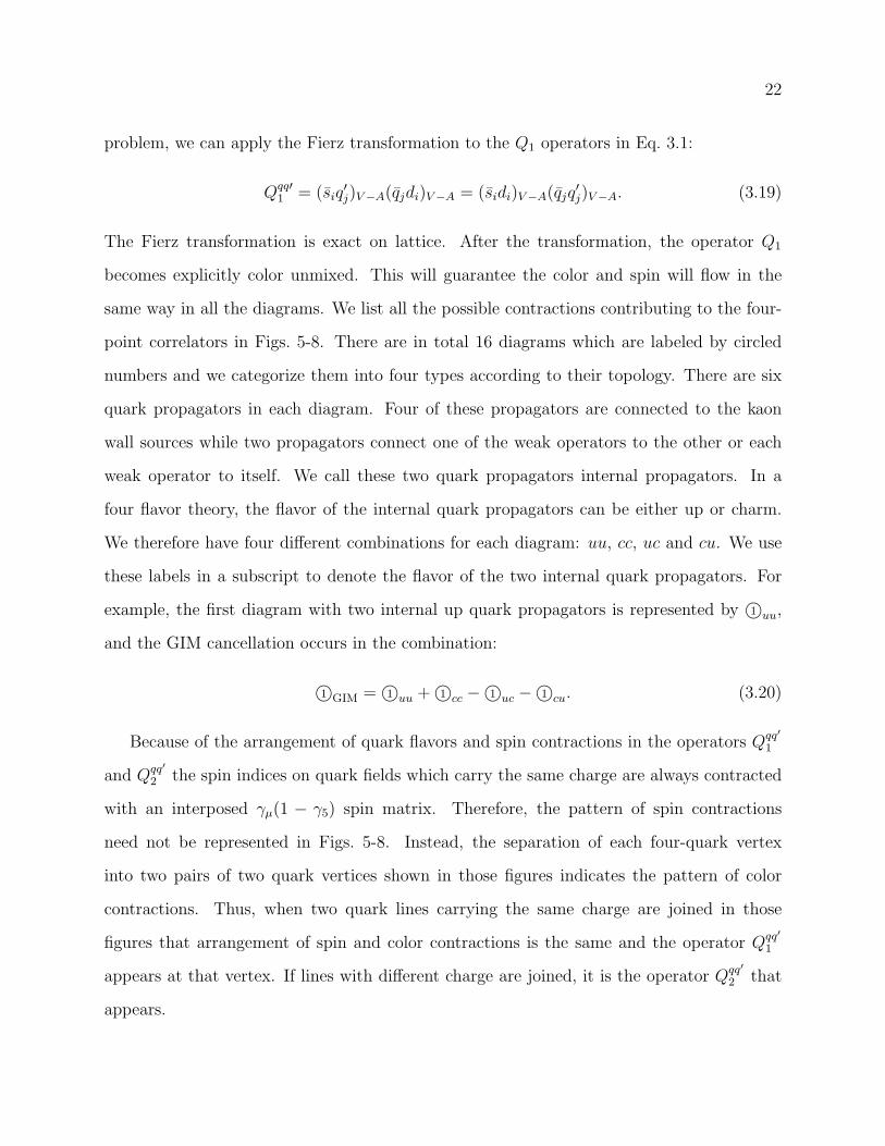
22
problem, we can apply the Fierz transformation to the Q1 operators in Eq. 3.1:
Qqq′1 = (siq
′j)V−A(qjdi)V−A = (sidi)V−A(qjq
′j)V−A. (3.19)
The Fierz transformation is exact on lattice. After the transformation, the operator Q1
becomes explicitly color unmixed. This will guarantee the color and spin will flow in the
same way in all the diagrams. We list all the possible contractions contributing to the four-
point correlators in Figs. 5-8. There are in total 16 diagrams which are labeled by circled
numbers and we categorize them into four types according to their topology. There are six
quark propagators in each diagram. Four of these propagators are connected to the kaon
wall sources while two propagators connect one of the weak operators to the other or each
weak operator to itself. We call these two quark propagators internal propagators. In a
four flavor theory, the flavor of the internal quark propagators can be either up or charm.
We therefore have four different combinations for each diagram: uu, cc, uc and cu. We use
these labels in a subscript to denote the flavor of the two internal quark propagators. For
example, the first diagram with two internal up quark propagators is represented by 1©uu,
and the GIM cancellation occurs in the combination:
1©GIM = 1©uu + 1©cc − 1©uc − 1©cu. (3.20)
Because of the arrangement of quark flavors and spin contractions in the operators Qqq′
1
and Qqq′
2 the spin indices on quark fields which carry the same charge are always contracted
with an interposed γµ(1 − γ5) spin matrix. Therefore, the pattern of spin contractions
need not be represented in Figs. 5-8. Instead, the separation of each four-quark vertex
into two pairs of two quark vertices shown in those figures indicates the pattern of color
contractions. Thus, when two quark lines carrying the same charge are joined in those
figures that arrangement of spin and color contractions is the same and the operator Qqq′
1
appears at that vertex. If lines with different charge are joined, it is the operator Qqq′
2 that
appears.
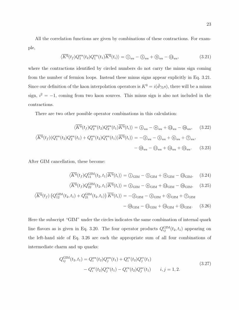
23
All the correlation functions are given by combinations of these contractions. For exam-
ple,
〈K0(tf )Quu1 (t2)Q
uu1 (t1)K0(ti)〉 = 1©uu − 5©uu + 9©uu − 13©uu, (3.21)
where the contractions identified by circled numbers do not carry the minus sign coming
from the number of fermion loops. Instead these minus signs appear explicitly in Eq. 3.21.
Since our definition of the kaon interpolation operators is K0 = i(dγ5s), there will be a minus
sign, i2 = −1, coming from two kaon sources. This minus sign is also not included in the
contractions.
There are two other possible operator combinations in this calculation:
〈K0(tf )Quu2 (t2)Q
uu2 (t1)K0(ti)〉 = 4©uu − 8©uu + 12©uu − 16©uu, (3.22)
〈K0(tf )(Quu1 (t2)Q
uu2 (t1) +Quu
2 (t2)Quu1 (t1))K0(ti)〉 = − 2©uu − 3©uu + 6©uu + 7©uu,
− 10©uu − 11©uu + 14©uu + 15©uu. (3.23)
After GIM cancellation, these become:
〈K0(tf )QGIM11 (t2, t1)K0(ti)〉 = 1©GIM − 5©GIM + 9©GIM − 13©GIM, (3.24)
〈K0(tf )QGIM22 (t2, t1)K0(ti)〉 = 4©GIM − 8©GIM + 12©GIM − 16©GIM, (3.25)
〈K0(tf )(QGIM
12 (t2, t1) +QGIM21 (t2, t1)
)K0(ti)〉 = − 2©GIM − 3©GIM + 6©GIM + 7©GIM
− 10©GIM − 11©GIM + 14©GIM + 15©GIM. (3.26)
Here the subscript “GIM” under the circles indicates the same combination of internal quark
line flavors as is given in Eq. 3.20. The four operator products QGIMij (t2, t1) appearing on
the left-hand side of Eq. 3.26 are each the appropriate sum of all four combinations of
intermediate charm and up quarks:
QGIMij (t2, t1) = Quu
i (t2)Quuj (t1) +Qcc
i (t2)Qccj (t1)
−Quci (t2)Q
cuj (t1)−Qcu
i (t2)Qucj (t1) i, j = 1, 2.
(3.27)
24
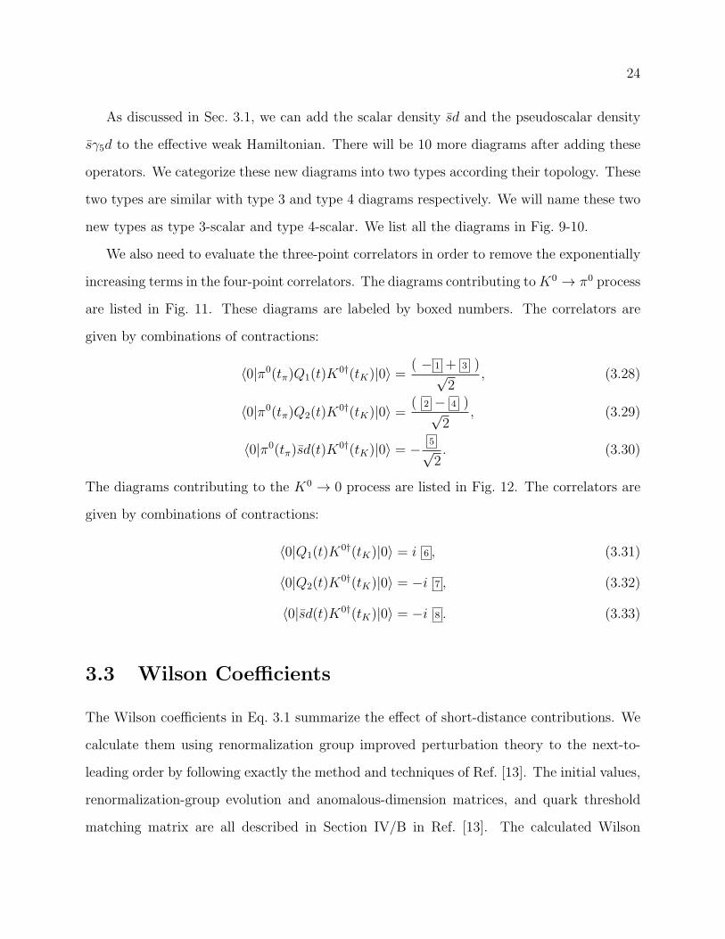
As discussed in Sec. 3.1, we can add the scalar density sd and the pseudoscalar density
sγ5d to the effective weak Hamiltonian. There will be 10 more diagrams after adding these
operators. We categorize these new diagrams into two types according their topology. These
two types are similar with type 3 and type 4 diagrams respectively. We will name these two
new types as type 3-scalar and type 4-scalar. We list all the diagrams in Fig. 9-10.
We also need to evaluate the three-point correlators in order to remove the exponentially
increasing terms in the four-point correlators. The diagrams contributing toK0 → π0 process
are listed in Fig. 11. These diagrams are labeled by boxed numbers. The correlators are
given by combinations of contractions:
〈0|π0(tπ)Q1(t)K0†(tK)|0〉 =
( − 1 + 3 )√2
, (3.28)
〈0|π0(tπ)Q2(t)K0†(tK)|0〉 =
( 2 − 4 )√2
, (3.29)
〈0|π0(tπ)sd(t)K0†(tK)|0〉 = − 5√
2. (3.30)
The diagrams contributing to the K0 → 0 process are listed in Fig. 12. The correlators are
given by combinations of contractions:
〈0|Q1(t)K0†(tK)|0〉 = i 6 , (3.31)
〈0|Q2(t)K0†(tK)|0〉 = −i 7 , (3.32)
〈0|sd(t)K0†(tK)|0〉 = −i 8 . (3.33)
3.3 Wilson Coefficients
The Wilson coefficients in Eq. 3.1 summarize the effect of short-distance contributions. We
calculate them using renormalization group improved perturbation theory to the next-to-
leading order by following exactly the method and techniques of Ref. [13]. The initial values,
renormalization-group evolution and anomalous-dimension matrices, and quark threshold
matching matrix are all described in Section IV/B in Ref. [13]. The calculated Wilson

25
coefficients at the renormalization energy scale µ = 2.15 GeV with 4 flavors are given in the
first two columns in Tab. 2. All the standard model parameters used in this calculation are
taken from PDG 2010 [4] and are also listed in Tab. 1.
Notice that to obtain the results in Tab. 2, we used the same strategy as in [13]: keep
only the leading order terms and discarding the other terms. For example, if we have an
expression (1 + aαs)(1 + bαs), we should not do the calculation by numerically multiplying
the two factors in the two parentheses. Instead, the expression is expanded, and only the
term 1 + (a + b)αs is kept and calculated. The initial condition, evolution operator matrix
and matching matrix are all functions of αs. We need to keep the analytical form, expand
the expressions, and keep only the O(1) and O(αs) term at the end. By following this
method, we were able to exactly reproduce the results in Ref. [13]. This is the advantage of
explicitly dropping all higher order terms: others can recognize exactly what kinds of terms
are dropped so the results can be easily reproduced exactly.
3.4 Non-perturbative Renormalization
In order to get ∆MK in physical units, we need to combine our lattice results with the Wilson
coefficients which describe the short-distance physics. However, the Wilson coefficients are
calculated in the MS scheme. So we need to convert the operators renormalized in MS scheme
into the lattice operators. We will discuss the details of this procedure in this section.
We will consider only the current-current operators defined in Eq. (3.3) which enter the
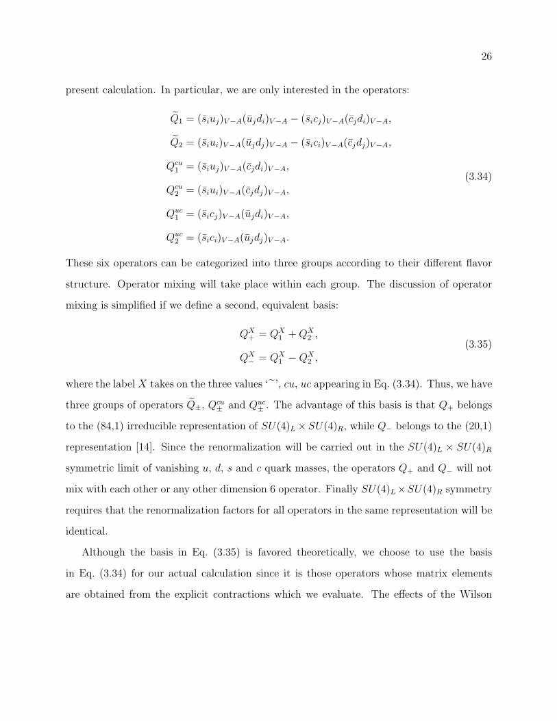
26
present calculation. In particular, we are only interested in the operators:
Q1 = (siuj)V−A(ujdi)V−A − (sicj)V−A(cjdi)V−A,
Q2 = (siui)V−A(ujdj)V−A − (sici)V−A(cjdj)V−A,
Qcu1 = (siuj)V−A(cjdi)V−A,
Qcu2 = (siui)V−A(cjdj)V−A,
Quc1 = (sicj)V−A(ujdi)V−A,
Quc2 = (sici)V−A(ujdj)V−A.
(3.34)
These six operators can be categorized into three groups according to their different flavor
structure. Operator mixing will take place within each group. The discussion of operator
mixing is simplified if we define a second, equivalent basis:
QX+ = QX
1 +QX2 ,
QX− = QX
1 −QX2 ,
(3.35)
where the labelX takes on the three values ‘˜’, cu, uc appearing in Eq. (3.34). Thus, we have
three groups of operators Q±, Qcu± and Quc
± . The advantage of this basis is that Q+ belongs
to the (84,1) irreducible representation of SU(4)L ×SU(4)R, while Q− belongs to the (20,1)
representation [14]. Since the renormalization will be carried out in the SU(4)L × SU(4)R
symmetric limit of vanishing u, d, s and c quark masses, the operators Q+ and Q− will not
mix with each other or any other dimension 6 operator. Finally SU(4)L×SU(4)R symmetry
requires that the renormalization factors for all operators in the same representation will be
identical.
Although the basis in Eq. (3.35) is favored theoretically, we choose to use the basis
in Eq. (3.34) for our actual calculation since it is those operators whose matrix elements
are obtained from the explicit contractions which we evaluate. The effects of the Wilson
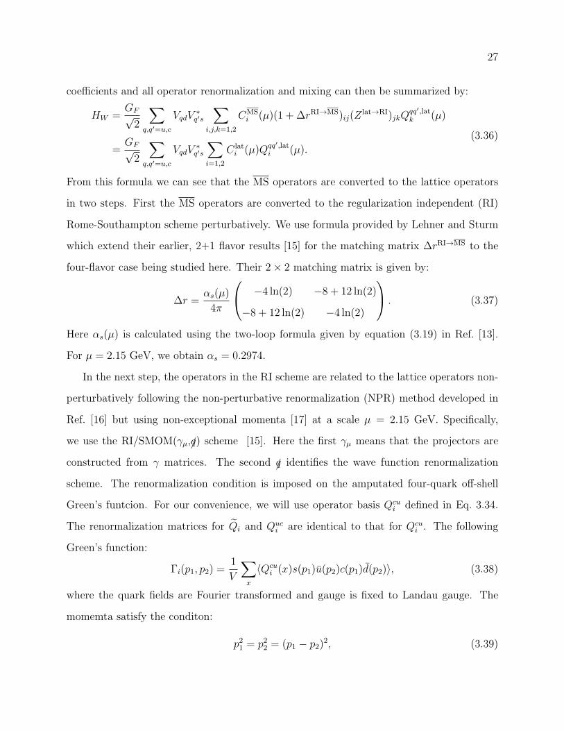
27
coefficients and all operator renormalization and mixing can then be summarized by:
HW =GF√2
∑
q,q′=u,c
VqdV∗q′s
∑
i,j,k=1,2
CMSi (µ)(1 + ∆rRI→MS)ij(Z
lat→RI)jkQqq′,latk (µ)
=GF√2
∑
q,q′=u,c
VqdV∗q′s
∑
i=1,2
C lati (µ)Qqq′,lat
i (µ).
(3.36)
From this formula we can see that the MS operators are converted to the lattice operators
in two steps. First the MS operators are converted to the regularization independent (RI)
Rome-Southampton scheme perturbatively. We use formula provided by Lehner and Sturm
which extend their earlier, 2+1 flavor results [15] for the matching matrix ∆rRI→MS to the
four-flavor case being studied here. Their 2× 2 matching matrix is given by:
∆r =αs(µ)
4π
−4 ln(2) −8 + 12 ln(2)
−8 + 12 ln(2) −4 ln(2)
. (3.37)
Here αs(µ) is calculated using the two-loop formula given by equation (3.19) in Ref. [13].
For µ = 2.15 GeV, we obtain αs = 0.2974.
In the next step, the operators in the RI scheme are related to the lattice operators non-
perturbatively following the non-perturbative renormalization (NPR) method developed in
Ref. [16] but using non-exceptional momenta [17] at a scale µ = 2.15 GeV. Specifically,
we use the RI/SMOM(γµ,/q) scheme [15]. Here the first γµ means that the projectors are
constructed from γ matrices. The second /q identifies the wave function renormalization
scheme. The renormalization condition is imposed on the amputated four-quark off-shell
Green’s funtcion. For our convenience, we will use operator basis Qcui defined in Eq. 3.34.
The renormalization matrices for Qi and Quci are identical to that for Qcu
i . The following
Green’s function:
Γi(p1, p2) =1
V
∑
x
〈Qcui (x)s(p1)u(p2)c(p1)d(p2)〉, (3.38)
where the quark fields are Fourier transformed and gauge is fixed to Landau gauge. The
momemta satisfy the conditon:
p21 = p22 = (p1 − p2)2, (3.39)

28
which is the non-exceptional momentum scheme. The Green’s function defined in Eq. 3.38
is given by products of momentum source propagators:
G1(p1, p2)abcdαβγδ =
1
V
∑
x,µ
e−2i(p2−p1)x{(
γ5S†(x, p1)γ5)aa′
γµ(1− γ5)S(x, p2)c′b}αβ
{(γ5S†(x, p1)γ
5)cc′
γµ(1− γ5)S(x, p2)a′d
}γδ
, (3.40)
G2(p1, p2)abcdαβγδ =
1
V
∑
x,µ
e−2i(p2−p1)x{(
γ5S†(x, p1)γ5)aa′
γµ(1− γ5)S(x, p2)a′b}αβ
{(γ5S†(x, p1)γ
5)cc′
γµ(1− γ5)S(x, p2)c′d}γδ
. (3.41)
Here S(x, p) is a propagator with a momentum source and a sink position x, the contraction
of color indices are given explicitly and the contraction of spin indices should follow the rule
of matrix multiplication inside each large curly bracket. We don’t specify the flavor of the
quark propagators in this formula since the renormalization condition is defined in the chiral
limit. The dependence of the results on the quark masses is usually extremely small. So we
use the same light quark mass for all flavors of quarks in our calculation and do not perform
a extrapolation to chiral limit.
Then we use the full quark propagator to amputate these Green’s functions:
Γi(p1, p2)abcdαβγδ = Gi(p1, p2)
a′b′c′d′
α′β′γ′δ′
(〈γ5S†(p1)γ
5〉−1)a′a′α′α
(〈S(p2)〉−1)b′bβ′β
(〈γ5S†(p1)γ
5〉−1)c′cγ′γ
(〈S†(p1)〉−1)d′d
δ′δ .
(3.42)
Here the quark propagator by S(p) =∑
x S(x, p)e−ipx. In order to define the renormalization
condition, we introduce the following spin-color projectors:
(P1)abcdαβγδ = [(1− γ5)γµ]αβ[(1− γ5)γµ]γδδ
adδcb, (3.43)
(P2)abcdαβγδ = [(1− γ5)γµ]αβ[(1− γ5)γµ]γδδ
abδcd. (3.44)
The operator mixing matrix is given by:
Mij = ΓiPj . (3.45)
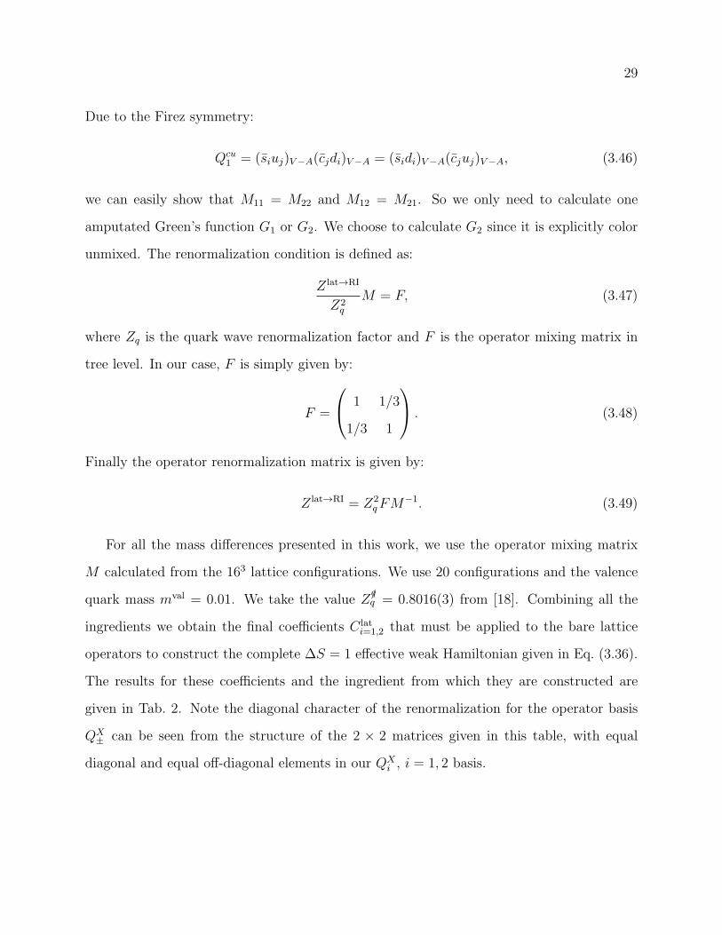
29
Due to the Firez symmetry:
Qcu1 = (siuj)V−A(cjdi)V−A = (sidi)V−A(cjuj)V−A, (3.46)
we can easily show that M11 = M22 and M12 = M21. So we only need to calculate one
amputated Green’s function G1 or G2. We choose to calculate G2 since it is explicitly color
unmixed. The renormalization condition is defined as:
Z lat→RI
Z2q
M = F, (3.47)
where Zq is the quark wave renormalization factor and F is the operator mixing matrix in
tree level. In our case, F is simply given by:
F =
1 1/3
1/3 1
. (3.48)
Finally the operator renormalization matrix is given by:
Z lat→RI = Z2qFM−1. (3.49)
For all the mass differences presented in this work, we use the operator mixing matrix
M calculated from the 163 lattice configurations. We use 20 configurations and the valence
quark mass mval = 0.01. We take the value Z/qq = 0.8016(3) from [18]. Combining all the
ingredients we obtain the final coefficients C lati=1,2 that must be applied to the bare lattice
operators to construct the complete ∆S = 1 effective weak Hamiltonian given in Eq. (3.36).
The results for these coefficients and the ingredient from which they are constructed are
given in Tab. 2. Note the diagonal character of the renormalization for the operator basis
QX± can be seen from the structure of the 2 × 2 matrices given in this table, with equal
diagonal and equal off-diagonal elements in our QXi , i = 1, 2 basis.
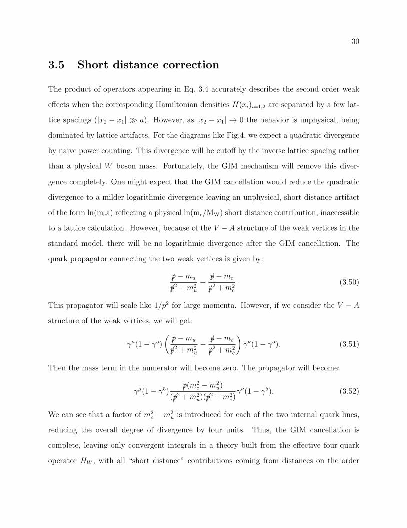
30
3.5 Short distance correction
The product of operators appearing in Eq. 3.4 accurately describes the second order weak
effects when the corresponding Hamiltonian densities H(xi)i=1,2 are separated by a few lat-
tice spacings (|x2 − x1| ≫ a). However, as |x2 − x1| → 0 the behavior is unphysical, being
dominated by lattice artifacts. For the diagrams like Fig.4, we expect a quadratic divergence
by naive power counting. This divergence will be cutoff by the inverse lattice spacing rather
than a physical W boson mass. Fortunately, the GIM mechanism will remove this diver-
gence completely. One might expect that the GIM cancellation would reduce the quadratic
divergence to a milder logarithmic divergence leaving an unphysical, short distance artifact
of the form ln(mca) reflecting a physical ln(mc/MW) short distance contribution, inaccessible
to a lattice calculation. However, because of the V −A structure of the weak vertices in the
standard model, there will be no logarithmic divergence after the GIM cancellation. The
quark propagator connecting the two weak vertices is given by:
/p−mu
/p2 +m2u
− /p−mc
/p2 +m2c
. (3.50)
This propagator will scale like 1/p2 for large momenta. However, if we consider the V − A
structure of the weak vertices, we will get:
γµ(1− γ5)
(/p−mu
/p2 +m2u
− /p−mc
/p2 +m2c
)γν(1− γ5). (3.51)
Then the mass term in the numerator will become zero. The propagator will become:
γµ(1− γ5)/p(m2
c −m2u)
(/p2 +m2u)(/p
2 +m2c)γν(1− γ5). (3.52)
We can see that a factor of m2c −m2
u is introduced for each of the two internal quark lines,
reducing the overall degree of divergence by four units. Thus, the GIM cancellation is
complete, leaving only convergent integrals in a theory built from the effective four-quark
operator HW , with all “short distance” contributions coming from distances on the order
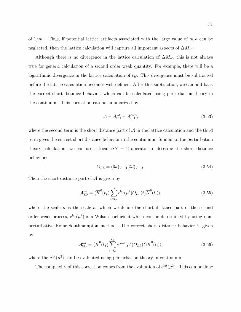
31
of 1/mc. Thus, if potential lattice artifacts associated with the large value of mca can be
neglected, then the lattice calculation will capture all important aspects of ∆MK .
Although there is no divergence in the lattice calculation of ∆MK , this is not always
true for generic calculation of a second order weak quantity. For example, there will be a
logarithmic divergence in the lattice calculation of ǫK . This divergence must be subtracted
before the lattice calculation becomes well defined. After this subtraction, we can add back
the correct short distance behavior, which can be calculated using perturbation theory in
the continuum. This correction can be summarized by:
A−AlatSD +Acont
SD , (3.53)
where the second term is the short distance part of A in the lattice calculation and the third
term gives the correct short distance behavior in the continuum. Similar to the perturbation
theory calculation, we can use a local ∆S = 2 operator to describe the short distance
behavior:
OLL = (sd)V−A(sd)V−A. (3.54)
Then the short distance part of A is given by:
AlatSD = 〈K0
(tf )
tb∑
t=ta
clat(µ2)OLL(t)K0(ti)〉, (3.55)
where the scale µ is the scale at which we define the short distance part of the second
order weak process, clat(µ2) is a Wilson coefficient which can be determined by using non-
perturbative Rome-Southhampton method. The correct short distance behavior is given
by:
AlatSD = 〈K0
(tf )
tb∑
t=ta
ccont(µ2)OLL(t)K0(ti)〉, (3.56)
where the clat(µ2) can be evaluated using perturbation theory in continuum.
The complexity of this correction comes from the evaluation of clat(µ2). This can be done
32
by evaluating the four quark, off-shell Greens function:
Γαβγδ(pi) = 〈sα(p1)dβ(p2)∫
d4x1
∫d4x2HW (x1)HW (x2)sγ(p3)dδ(p4)〉. (3.57)
Here the quark fields are Fourier transformed and gauge is fixed to Landau gauge. The
momentum of the quarks should satisfy p2i = µ2. Also, the pi should be chosen appropriately
so that all the internal momenta contributing to Γ(pi) will be at the scale µ. The value for
µ should satisfy:
ΛQCD ≪ µ ≪ π
a. (3.58)
Then we evaluate second Greens function for the local OLL operator:
ΓSDαβγδ(pi) = 〈sα(p1)dβ(p2)
∫d4xOLL(x)sγ(p3)dδ(p4)〉. (3.59)
This Green’s function describes the short distance component of Γ(pi). For a large enough
µ, Γ(pi) will be dominated by short distance effect. Thus, the Wilson coefficients clats (µ2)
can be determined by:
(Γampαβγδ(pi)− clats (µ2)Γamp,SD
αβγδ (pi))Pαβγδ = 0, (3.60)
where “amp” means that the Green functions should be amputated, Pαβγδ is a spin and color
projector
Pαβδγ =((1− γ5)γµ
)αβ
((1− γ5)γµ
)γδ
(3.61)
3.6 Finite volume corrections
In this section, we will discuss the finite volume effects in the mass difference calculation.
Finite volume effects exist in all lattice calculations. If there are no multi-particle states
evolved, the finite volume effects will usually decrease exponentially as the lattice size L
increases. We usually neglect such effects in the practical calculation. However, in the mass
difference calculation, there will be lots of multi-particle intermediate states contributing to
33
the mass difference defined in Eq. 3.8. These states may be distorted in a finite volume and
will introduce errors which are suppressed only by power of L. The finite volume effects
have been studied in detail in Ref. [11]. The starting point is Luscher’s relation [19] between
finite-volume two-particle energy, E = 2√m2
π + k2 and the two-particle scattering phase
shift δ(E):
φ(kL
2π) + δ(E) = nπ, (3.62)
where n is an integer and the known function φ(q) is defined in Ref. [19]. This relation
connects the π-π energy in finite volume with the phase shift in the infinite volume. We
want to use this condition to relate ∆MK computed in finite volume and infinite volume.
We can choose a specially tuned lattice volume so that there is an π-π state |n0〉 with energy
En0nearly degenerate with mK . The KS ↔ ππ system can be described by the degenerate
perturbation theory. For simplicity we will assume CP symmetry so that π-π will only couple
to the KS state. Following second order degenerate perturbation theory, we can obtain the
energies of KS and the two pion state |n0〉 as the eigenvalues of the 2× 2 matrix:
mK +
∑n 6=n0
|〈n|HW |KS〉L|2
mK−En〈KS|HW |n0〉L
〈n0|HW |KS〉L En0+∑
n 6=KS
|〈n|HW |n0〉L|2
En0−En
. (3.63)
The subscript L here means the matrix elements are evaluated in finite volume. Finite and
infinite volume quantities can then be related by requiring that the eigenvalue of the 2 × 2
matrix in Eq. 3.63 solve Eq. 3.62. The infinite volume phase shift δ(E) is the sum of that
arising from the strong interaction, δ0(E), a resonant contribution from the KS pole and the
second-order Born terms:
δ(E) = δ0(E) + arctan
(Γ(E)/2
mK +∆mKs− E
)− π
∑
β 6=KS
|〈β|HW |ππ(E)〉|2E − Eβ
. (3.64)
Here Γ(E) is proportional to the square of the KS-ππ vertex which becomes the KS width
when evaluated at E = mK :
Γ(E) = 2π|〈ππ(E)|HW |KS〉|2, (3.65)
34
where for the two-pion state we choose the normalization 〈ππ(E)|ππ(E ′)〉 = δ(E − E ′).
The easiest case to examine is that in which the energy difference En0−mK is very small
compared with mK but large compared to ∆MK or Γ, so that En0and mK are not exactly
degenerate. With this choice, the π-π energy eigenvalue determined from Eq. 3.63 differs
from En0by the usual second order perturbation theory expression:
Eππ = En0+
|〈KS|HW |n0〉L|2En0
−MK
+∑
n 6=KS
|〈n|HW |n0〉L|2En0
− En
. (3.66)
Combining this expression with Eq. 3.62 and Eq. 3.64 and equating all terms of second order
in HW yeilds the relation:
∂(φ+ δ0)
∂E
{|〈KS|HW |n0〉L|2
En0−MK
+∑
n 6=KS
|〈n|HW |n0〉L|2En0
− En
}=
Γ(En0)/2
En0−mK
+π∑
β 6=KS
|〈β|HW |ππ(E)〉|2E − Eβ
.
(3.67)
This expression has two useful consequences. First we can equate the residues of the
kaon poles, En0= mK on the left- and right-hand sides. This gives us the original Lellouch-
Luscher relation. Second we can subtract the pole terms and equate the remaining parts
of Eq. 3.67 evaluated at En0= mK . This second result will be used below to remove the
second-order Born terms.
Now we are ready to the examine a more complicated case in which En0= mK . The
finite volume energies are still given by the eigenvalues of Eq. 3.63:
E± = mK ± 〈n0|HW |KS〉+1
2
{∑
n 6=n0
|〈n|HW |KS〉L|2mK − En
+∑
n 6=KS
|〈n|HW |n0〉L|2mK − En
}, (3.68)
but now the eigenstates are equal mixtures of the degenerate K and finite volume π-π state
|n0〉. We again require that these finite-volume energies satisfy Eq. 3.62. Expanding to
second order of HW , we get the relation between the finite and infinite volume expressions
for the KS mass shift:
∆mKS=
∑
n 6=n0
|〈n|HW |KS〉L|2mK − En
−∂2(φ+ δ0)/∂E2
2∂(φ+ δ0)/∂E|〈n0|HW |KS〉L|2−
∂|〈n0|HW |KS〉L|2∂E
, (3.69)
35
where Eq. 3.67, evaluated at En0= mK with the pole term subtracted has been used to
eliminate the second-order Born terms.
Finally, the infinite-volume KL − KS mass difference can be obtained as follows. First
observe that the KL second order mass shift is given by a formula similar to Eq. 3.69 in
which KL replaces KS and all but the first term on the right-hand side are omitted since KL
does not couple to two pions in our approximation of CP symmetry. Subtracting this new
formula from Eq. 3.69 gives:
∆mK = ∆mFVK − ∂2(φ+ δ0)/∂E
2
2∂(φ+ δ0)/∂E|〈n0|HW |KS〉L|2 −
∂|〈n0|HW |KS〉L|2∂E
(3.70)
Here ∆mFVK is defined in Eq. 3.8. The correction terms in this formula are all accessible in a
lattice calculation. However, in our numerical work, we are not able to identify a clear signal
from two pion intermediate states. So we are not able to study their finite volume effects in
this work. In a future calculation at physical kinematics, the finite volume effects may be
important and should be furthur studied.

Chapter 4
Measurement methods
In this chapter, we will discuss the techniques used in the lattice calculation of ∆MK . In Sec-
tion. 4.1, we will discuss the different sources of the quark propagators. In Section. 4.2, we will
discuss the low-mode-deflation method based on the EigCG and Lanczos algorithms. Sec-
tion 4.3 discuss the two-point and three-point correlators in our calculation. In Section. 4.4,
we explain the strategies used to calculate the different type of diagram contributing to the
four-point correlators. In Section. 4.5, we briefly summarize the data analysis techniques.
4.1 Propagator sources
The contractions shown in Chapter. 3 can be written as products of quark propagators. We
need to compute all the needed quark propagators in order to evaluate these contractions.
A quark propagator from the source point y to the sink point x is given by:
S(x, y) = D−1(x, y), (4.1)
where S(x, y) is a 12×12 spin-color matrix, D is the Dirac matrix on lattice. For a resonantly
large lattice, it is impossible to invert the Dirac matrix since the dimension of the matrix
is extremely high. So we are not able to compute S(x, y) for all source and sink locations.
36
37
However, in most cases, it is sufficient to calculate the quark propagator for some specific
choices of source. A general source b(x) can be any function of space-time. The propagator
for this source is given by:
S(x) =∑
y
S(x, y)b(y). (4.2)
This propagator can be obtained by solving the following linear system:
∑
y
D(x, y)S(y) = b(x). (4.3)
A important property of S(x, y) is γ5-hermiticity. In our domain wall fermion formalism,
the dirac matrix satisfies D† = γ5Dγ5. Hence the propagator should satisfy:
S(y, x) = γ5S(x, y)†γ5. (4.4)
This relation can tell us S(y, x) immediately after S(x, y) has been computed.
The choice of sources depends on the specific problem. The point source b(x) is 1 at the
source point and a specific spin and color and 0 anywhere else. The propagator given by
Eq. 4.1 is a point source propagator from source location y. We will use point sources for
the two internal propagators in the type 1 and type 2 contractions given in Section. 3.2.
To better overlap with the ground state, we use wall source for the kaon and pion inter-
polating field. The wall source at time t with spin α and color a is defined as:
b(~y, ty) =
χaα, ty = t
0, ty 6= ty,
(4.5)
where χaα is a 12-component vector with 1 at spin α and color a and 0 at anywhere else.
The corresponding wall source propagator is given by:
SW (~x, tx; ty) =∑
~y
S(~x, tx; ~y, ty). (4.6)
38
Sometimes we will need a wall-source-wall-sink propagator. It is obtained by summing over
the sink position:
SWW (tx; ty) =∑
~x,~y
S(~x, tx; ~y, ty). (4.7)
In the type 3 and type 4 diagrams given in Section. 3.2, we have some fermion loops in
the contractions. So we need to calculate S(x, x) for all possible x. Naively, we can calculate
a point source propagators at each possible source location. However, this is impossible in
practice since there are too many source locations. The solution is to use random wall source
propagators to give a unbiased estimation for the fermion loops. The random wall source at
time t and spin α and color a is given by:
b(~y, ty) =
χaαη(~y, ty), ty = t
0, ty 6= t,
(4.8)
where χaα is a 12-component vector with 1 at spin α and color a and 0 at anywhere else,
η~y,ty are random numbers satisfying:
〈η†(~x, tx)η(~y, ty)〉 = δ(~x− ~y)δ(tx − ty), (4.9)
where 〈· · · 〉 means average for many hits of random numbers. The random wall source
propagators is given by:
SRW (~x, tx; ty) =∑
~y
S(~x, tx; ~y, ty)η(~y, ty). (4.10)
Finally the fermion loops are given by:
S(~x, tx; ~x, tx) =∑
η
SRW (~x, tx; tx)η†(~x, tx) (4.11)
In our operator renormalization calculation, we use a volume momentum source. This
source is defined as b(y) = eipy. The momentum source propagator is then given by:
S(x; p) =∑
y
S(x, y)eipy. (4.12)
39
The momentum-source-momentum-sink propagator is defind as:
S(p) =∑
x,y
S(x, y)e−ip(x−y). (4.13)
4.2 Low Mode Deflation
Solving for the quark propagators is the most expensive part of our calculation. We use the
conjugate gradient (CG) methods to solve the linear system:
Dx = b (4.14)
The conjugate gradient method can’t be applied directly here since it requires D to be
Hermitian. So the equation we actually solve is the normal equation:
D†Dx = D†b = b′ (4.15)
The convergence of the CG algorithm is controlled by the condition number κ(D†D), which
is given by the ratio between the largest and the smallest eigenvalues of D†D. The CG
algorithm converges faster for a smaller κ. κ(D†D) for the light quark is larger than the
value for the heavy quark. So a light quark CG solver needs more iteration steps to converge.
A straightforward method to reduce κ is the low-mode-deflation method. If we know lowest
n eigenvalue and eigenvectors of D†D, we can define a projection operator:
P =n∑
i=1
|λi〉〈λi| (4.16)
where λi is the i-th smallest eigenvalue and |λi〉 is the corresponding eigenvector. Since P
commutes with D†D, the normal equation 4.15 can be split into decoupled equations:
(D†D)‖x‖ =b‖, x‖ = Px, b‖ = Pb (4.17)
(D†D)⊥x⊥ =b⊥, x⊥ = Px, b⊥ = Pb (4.18)
40
where (D†D)‖ = PD†DP and (D†D)⊥ = (1 − P )D†D(1 − P ) are referred to as the little
operator and the deflated operator respectively.
The solution to the little system 4.17 is simply given by:
x‖ =n∑
i=1
|λi〉〈λi|b〉λi
. (4.19)
The deflated system 4.18 can be solved using the CG algorithm. The new condition number
κ(D†D)⊥ =λ1
λn+1
κ(D†D) (4.20)
is reduced and one expects the solver to be accelerated.
The deflation method usually works well for the light quark CG solver and works poorly
when the quark mass is heavy. This can be explained by the ratio λn/λ1. For light quark,
this ratio is usually large. When the quark mass becomes heavy, the spectrum of the low
eigenvalues is bounded from below by the large quark mass. Thus this ratio will become
smaller for a heavier quark mass. In our lattice calculation, we only use low mode deflation
only for the up and down quark CG solver. For the strange and charm quark propagator,
we will use the plain CG algorithm.
The calculation of the low-lying eigenvectors can be expensive. However, in our calcula-
tion, we need to solve Eq. 4.15 for many different sources. We can use the same eigenvectors
for CG solver with the same quark mass. Hence the time spent on calculating eigenvectors
is amortized and is only a small part of the total time.
There are two different method to calculate the low modes: the EigCG algorithm and
the implicit restarted Lanczos (IRL) algorithm. The details of the EigCG algorithm can be
found in Ref. [1]. The EigCG algorithm builds an explicitly restarted Lanczos algorithm on
top of the conjugate gradient method. The idea is to reuse the search directions generated
by the conjugate gradient algorithm to compute the necessary Lanczos vectors. It does not
require additional matrix-vector multiplications. So the increase in the time cost is small.
Since the Lanczos algorithm is numerically unstable, it also restarts itself when a certain
41
number of eigenvectors obtained. A certain number of new eigenvectors will be calculated in
each EigCG solver. At the beginning of a EigCG solver, we can use the already calculated
eigenvectors to do deflation, thus accelerating the solver. A new solver will not only collect
more eigenvectors but also will improve the precision of the already calculated eigenvectors.
Gradually, the solver will become faster and faster. Finally we stop collecting eigenvectors
and simply do deflation to speed up the solver.
In Ref. [2], Qi observed a clear slowing-down point (around res ≈ 10−6) on the conver-
gence curve for the sped-up solver. This was due to the inaccuracy of the eigenvectors we
obtained from EigCG solvers. Qi’s strategy was to do multiple projections by restarting the
CG algorithm using the residual of previous inversion as the new right hand side. Qi found
that a single restart point at res ≈ 10−5 can solve the slowing-down problem if our target
precision is 10−8. With this restart technique, in our 163 lattice calculation with a 412 MeV
pion mass, we obtain a factor of 6 speed up using 100 low-lying eigenvectors calculated by
the EigCG algorithm.
The IRL algorithm is a standard textbook algorithm which can calculate the eigenvec-
tors of hermitian matrix to machine precision. The details of this algorithm are discussed in
Ref. [3]. This algorithm can give more precise eigenvectors which can provide better deflation
effects. However, unlike EigCG, the IRL algorithm needs many extra Dirac matrix multipli-
cation and is more expensive. A Chebyshev polynomial is used to change the spectrum of
the Dirac matrix and thereby to accelerate the IRL algorithm. In our 243 lattice calculation
with a 330 MeV pion mass, the number of propagators we need to calculate is much greater
than were required for the 163 calculation. To get a better deflation effect, we use the IRL
algorithm to calculate 300 exact eigenvectors and get a factor of 8 speed up.
42
4.3 Two-point and three-point correlators
Two-point correlator are usually calculated to extract meson masses. The correlator is given
by:
C(t1, t2) = 〈O(t2)O†(t1)〉, (4.21)
where O is the interpolating field for the meson. After inserting a set of QCD energy
eigenstates, one obtains:
C(t1, t2) =∑
n
〈0|O|n〉e−En(t2−t1)〈n|O†|0〉
t2≫t1= N2me
−Em(t2−t1), (4.22)
where |m〉 is the lowest energy eigenstate which can couple to O and Nm = |〈0|O|m〉| is
the normalization factor of the interpolating field. We can obtain the meson mass and the
normalization factor of the interpolating field from a simple exponential fit. There are many
choices of the meson interpolating field. We use a wall source in our calculation. For example,
the wall source kaon interpolating filed can be written as:
OK0(t) = i∑
~x,~y
s(~x, t)γ5d(~y, t). (4.23)
The wall source is not explicitly gauge invariant. This can be solved by fixing the gauge field
at time t to Coulomb gauge. A Coulomb gauge fixed wall source has better overlap with
the ground state of kaon than a plain point source. We find that a Coulomb gauge fixed
wall source works well in both our 163 and 243 calculations. However, in a larger volume, a
Coulomb gauge fixed wall source kaon can be much larger than the size of a physical kaon.
So it may be better to use a more localized source in future calculation on larger lattices.
We also use a two-point correlator to extract the matrix element 〈0|O|K0〉. The correlator
can be written as:
C(t1, t2) = 〈O(t2)K†(t1)〉. (4.24)
43
We have listed the needed diagrams in Fig. 12. It is convenient to define the ratio:
R(t1, t2) =〈O(t2)K
†(t1)〉〈K(t2)K†(t2)〉
=1
NK
〈0|O|K0〉, (4.25)
where NK is the kaon normalization factor and the second equality is valid for sufficiently
large t2 − t1. The plateau value for R(t1, t2) will give us 〈0|O|K0〉.
The three-point correlator is used to compute the matrix element 〈π0|O|K0〉. The corre-
lator can be written as:
C(t1, to, t2) = 〈π0(t2)O(to)K(t1)†〉. (4.26)
We have listed the possible diagrams in Fig. 11. We can define the ratio:
R(t1, tO, t2) =〈π0(t2)O(to)K(t1)
†〉〈π0(t2)π(to)†〉〈K(to)K(t1)†〉
=〈π0|O|K0〉NKNπ
, (4.27)
where NK is the kaon normalization factor, Nπ is the pion normalization factor and the
second equality is valid for sufficiently large t2− t1. Again 〈π0|O|K0〉 is given by the plateau
in R(t1, tO, t2) as a function of tO for sufficiently large |t2 − t1|.
4.4 Evaluation of four-point correlators
The four-point correlators can be written as combinations of the contractions listed in Fig. 5-
8. Each contraction is composed of six quark propagators. In order to make our discussion
more concrete, we will discuss some example here. The contraction 1© in Fig. 5 is written
as:
1©uu =Tr(γµ(1− γ5)LW (x, ti)γ5γ5SW †(x, ti)γ
5)Tr(γν(1− γ5)L(y, x)γµ(1− γ5)L(x, y))
Tr(γν(1− γ5)LW (y, tf )γ5γ5SW †(y, tf )γ
5). (4.28)
44
The two kaon wall sources are located at ti and tf . The two weak Hamiltonian densities are
located at x and y. L(x, y) is a point source propagator from y to x. LW (x, t) is a light
quark propagator with Coulomb gauge fixed wall source at time t and sink at space time
position x. SW (x, t) is similar but for strange quark. We also use the γ5-hermiticity for the
strange quark wall source propagators. For simplicity we only give the contraction for the
case that both internal quarks are up, the other cases are very similar.
Another useful example is contraction 9©:
9©uu =Tr(γµ(1− γ5)LW (x, ti)γ5γ5SW †(x, ti)γ
5γν(1− γ5)LW (y, tf )γ5γ5SW †(y, tf )γ
5)
Tr(γµ(1− γ5)LRW (x, tx)η†(x))Tr(γν(1− γ5)LRW (y, ty)η
†(y)). (4.29)
Here LRW (x, t) is a light quark propagator with random wall source at time t and sink
at space-time position x. The fermion loop L(x, x) is replaced with LRW (x, tx)η†(x) this
expression. All the contractions can be written down similarly. We give all the expression
in Appendix. A.
We use a different strategy to calculate type 1,2 and type 3,4 diagrams. This is due to the
different topologies of these contractions. We will discuss the evaluation of type 1,2 diagram
first. For given values of tx and ty, each of the two effective operators should be integrated
over the whole spatial volume. However, there is no easy way to do this because of two
difficulties. First, we are not able to compute all of the light-quark propagators connecting
the two operators. It is impractical to use point source propagators since there will be V
point sources on each time slice. In simpler cases, this difficulty can be avoided by the
use of a stochastic source distributed over the time slice. However, an attempt to use this
technique in the present case failed to give a signal that could be recognized above the noise.
Even if this first difficulty of generating the multitude of needed point source propagators
could be overcome, we would still face a second difficulty: the number of operations needed
to calculate all the contractions would be O(V 2), where V is the space-time volume of the
lattice. This also would be too time consuming. Thus, we sum the location of only one of
45
the two operators over the spatial volume and, relying on the translational symmetry of the
other ingredients in the calculation, fix the spatial location of other operator at the origin
(0, 0, 0). For each of the contractions in our calculation, these two weak operators enter in
distinct ways and we average the two cases where one operator is fixed at the origin and the
other integrated over the spatial volume to improve the statistics.
For type 3,4 contractions, the situation is very different. There are no propagators con-
necting the two weak Hamiltonian densities. We can use random wall source propagators to
evaluate the fermion loops. Also, the number of operations needed to calculate the contrac-
tions is O(V ) instead of O(V 2). The reason is that we can always write the contractions as
the product of two independent parts. Each part will only need O(V ) time to compute. For
type 3 diagrams in Fig. 7, the contractions can be split into an upper half and a lower half.
For type 4 diagrams in Fig. 8, we can split the contractions into a left half and a right half.
The subtraction diagrams shown in Fig. 9-10 can be calculated similarly.
4.5 Data Analysis
After we have calculated all the correlation functions like C(t) for the meson from N config-
urations, we usually need to fit the data to some specific function form f(t, θ) as in Eq. 4.22.
This is accomplished by minimizing the correlated χ2,
χ2 =∑
t,t′
[f(t, θ)− C(t)]V −1(t, t′)[f(t′, θ)− C(t′)], (4.30)
where V (t, t′) is the covariance matrix for C(t),
V (t, t′) =1
N(N − 1)
N∑
i=1
(C i(t)− C(t))(C i(t′)− C(t′)). (4.31)
If the functional form fits the data well, we will get a χ2 per degree of freedom (χ2/d.o.f)
around 1. A large χ2/d.o.f usually suggests a poor fit. The most common reason is that
the fitting model does not describe the data well. For example, we will usually find a large
46
χ2/d.o.f if we include data from the case in which the meson source and the meson sink are
too close. There will be contamination from excited states and we will be unable to fit all
the data with a single exponential term. To improve the quality of fit, we can either drop
these data points or add another exponential term into the fitting formula. Another reason
for large χ2/d.o.f is that the covariance matrix is so singular that the fitting does not work
properly. In that case, we can turn to an uncorrelated fit. The χ2 minimized in uncorrelated
fit is given by:
χ2 =∑
t
[f(t, θ)− C(t)
σ(t)]2, (4.32)
where σ2(t) =∑N
i=1(Ci(t) − C(t))2/N . We can see that the uncorrelated fit uses only the
diagonal terms in the correlation matrix. Hence the correlation between difference data
points are not taken into account. The χ2 values in the uncorrelated fit are usually very
small and not very meaningful.
If the data are strongly correlated, it is usually better to use the correlated fit which
may give a more accurate result and a clear meaning for the χ2. In some cases, we will get
significantly smaller error bar with the correlated fit than the uncorrelated fit. However,
for simplicity, we can just use an uncorrelated fit for simple exponential or cosh fits for the
mesons since it usually gives equally good results.
The correlated or uncorrelated fit gives us the central value only. We usually use the
jackknife method to compute the error on the fitting parameters. Let Ci(t) to stand for the
correlation function we calculated from the configuration number i, and we have a sample
of N configurations S = {Ci(t), i = 1 . . . N}. Based on the correlated fit or uncorrelated fit
from the previous discussion, we can compute the parameter θ. Let us label it as θ = g(S).
The jackknife method is :
1. Obtain N samples from S by leaving one out a time: S−i, for i=1, . . ., N.
2. For each such sample, fit the parameter θ and determine the value θi = g(S−i).
47
3. Compute the average of θi: θ. The square of the error on θ is estimated as
σ2J =
N − 1
N
N∑
i=1
(θi − θ)2. (4.33)
Chapter 5
Results from the 163 × 32× 16 Lattice
In this chapter, we will discuss the results from the 163×64×16 lattice ensemble. Section. 5.1
gives the details of the simulation. In Section. 5.2, we discuss the short distance effects
and the GIM cancellation. In Section. 5.3, we discuss the long distance effects for each
definite parity channels separately. Section. 5.4 gives the mass difference results in physical
units. In Section. 5.5, we compare our lattice calculation with the NLO perturbation theory
calculation.
5.1 Simulation Details
The calculation is performed on a lattice ensemble generated with the Iwasaki gauge action
and 2+1 flavors of domain wall fermions at a coupling β = 2.13. The space-time volume is
163 × 32 and the inverse lattice spacing a−1 = 1.729(28)GeV. The fifth-dimensional extent
is Ls = 16 and the residual mass is mres = 0.00308(4) in lattice units. The sea light and
strange quark masses are ml = 0.01 and ms = 0.032 respectively, corresponding to a pion
mass Mπ = 421MeV and a kaon mass MK = 563MeV. We use 800 configurations, each
separated by 10 time units. This ensemble is described in greater detail in Ref. [18] and
is also similar to the earlier ensembles described and analyzed in Ref. [20], except that the
48
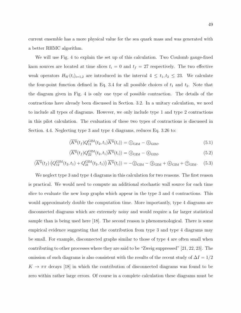
49
current ensemble has a more physical value for the sea quark mass and was generated with
a better RHMC algorithm.
We will use Fig. 4 to explain the set up of this calculation. Two Coulomb gauge-fixed
kaon sources are located at time slices ti = 0 and tf = 27 respectively. The two effective
weak operators HW (ti)i=1,2 are introduced in the interval 4 ≤ t1, t2 ≤ 23. We calculate
the four-point function defined in Eq. 3.4 for all possible choices of t1 and t2. Note that
the diagram given in Fig. 4 is only one type of possible contraction. The details of the
contractions have already been discussed in Section. 3.2. In a unitary calculation, we need
to include all types of diagrams. However, we only include type 1 and type 2 contractions
in this pilot calculation. The evaluation of these two types of contractions is discussed in
Section. 4.4. Neglecting type 3 and type 4 diagrams, reduces Eq. 3.26 to:
〈K0(tf )QGIM11 (t2, t1)K0(ti)〉 = 1©GIM − 5©GIM, (5.1)
〈K0(tf )QGIM22 (t2, t1)K0(ti)〉 = 4©GIM − 8©GIM, (5.2)
〈K0(tf )(QGIM
12 (t2, t1) +QGIM21 (t2, t1)
)K0(ti)〉 = − 2©GIM − 3©GIM + 6©GIM + 7©GIM. (5.3)
We neglect type 3 and type 4 diagrams in this calculation for two reasons. The first reason
is practical. We would need to compute an additional stochastic wall source for each time
slice to evaluate the new loop graphs which appear in the type 3 and 4 contractions. This
would approximately double the computation time. More importantly, type 4 diagrams are
disconnected diagrams which are extremely noisy and would require a far larger statistical
sample than is being used here [18]. The second reason is phenomenological. There is some
empirical evidence suggesting that the contribution from type 3 and type 4 diagrams may
be small. For example, disconnected graphs similar to those of type 4 are often small when
contributing to other processes where they are said to be “Zweig suppressed” [21, 22, 23]. The
omission of such diagrams is also consistent with the results of the recent study of ∆I = 1/2
K → ππ decays [18] in which the contribution of disconnected diagrams was found to be
zero within rather large errors. Of course in a complete calculation these diagrams must be
50
calculated explicitly after which the precision of the Zweig suppression will be known.
As discussed in Sec. 3.1, we need to calculate the matrix elements 〈π0|HW |K0〉 and
〈0|HW |K0〉 in order to remove the exponentially growing terms in the second order correlator.
In this non-unitary calculation, there will be no contribution from vacuum intermediate state.
Also the definition of the π0 intermediate state must be reconsidered. In a unitary theory, uu,
dd and ss will mix with each other through disconnected diagrams. Then the resulting energy
eigenstates are π0, η and η′, where π0 is defined as i(uγ5u− dγ5d)/√2. However, in our non-
unitary calculation, all disconnected diagrams are neglected and correlators of the operators
i(uγ5u± dγ5d) will reveal independent but symmetrical “states” with the same mass. Since
only up quarks can appear in our intermediate state, we must use the interpolating operator
iuγ5u to create our π0 state and can neglect the effects of the symmetrical state created by
dγ5d. Thus, in our calculation of 〈π0|HW |K0〉, we use π0 = iuγ5u (with no 1/√2 factor) and
only include contraction 1 and 2 shown Fig. 11.
We use periodic boundary conditions in the spatial directions for the Dirac operator when
computing the propagators. In the temporal direction, we calculate propagators for both
periodic and anti-periodic boundary conditions and take their average for the propagator that
we use. This effectively doubles the temporal extent of the lattice and suppresses around-
the-world effects to a negligible level. (This approach is equivalent to working on a lattice of
size 163×64 with gauge fields invariant under a translation of 32 sites in the time direction.)
The most expensive part of this simulation is solving for the light quark propagators. There
are 2 wall source light quark propagators and 20 point source light quark propagators, one on
each time slice between ta = 4 and tb = 23. So in total we need to calculate (20+2)×2 = 44
propagators, where the factor of two comes from our two choices of temporal boundary
conditions. Further each propagator requires 12 Dirac operator inversions, one for each spin
and color. This large number of light-quark Dirac operator inversions makes this calculation
a good candidate for the use of the EigCG technique [1, 2]. We collect the lowest 100
51
eigenvectors and use them to accelerate the light-quark Dirac operator inversions. The
overhead associated with collecting these low modes is amortized over many inversions and
the number of conjugate gradient iterations is reduced by a factor of 6. The parameters for
the EigCG algorithm is given in Tab. 5. For the strange and charm quark propagators, we
use the plain CG solver. We use a 10−8 stopping condition for all the CG and EigCG solvers.
The time separation between the kaon wall source and the ∆S = 1 weak operators
should be large enough to project onto kaon states. In the set up of this calculation, the two
operators can be located at any time slice between [4, 23]. So the time separation between the
kaon source or sink and either effective weak operator is guaranteed to be equal or larger than
4. In Fig. 13 we give a sample kaon effective mass plot for ml = 0.01 and ms = 0.032. This
plot suggests that the effects of excited kaon states will be negligible when the separation
between source and sink is 5 or larger. We therefore use the restricted range [5, 22] for tk in
the following analysis, discarding the results when either operator is at the location tk = 4
or 23 for k = 1 and 2.
In order to reduce short distance effects to a level which can be accurately controlled
using lattice methods, we introduce a valence charm quark into our calculation. We will
use six different charm quark masses in order to investigate the resulting GIM cancellation.
These masses are given in Tab. 3, where we use the mass renormalization factor ZMSm (2
Gev)=1.498 [24]. When we discuss the long distance effects in Sec. 5.3, we choose a 863MeV
valence charm quark mass and several different valence strange quark masses. The strange
quark masses and corresponding kaon masses are given in Tab. 4. The up and down quark
masses are kept at their unitary value, equal to the 0.01 mass of the sea quark.
5.2 Short Distance Contribution
In this section, we discuss the short distance contribution to our calculation of ∆MK in
detail. We begin by discussing results without a charm quark and their dependence on a
52
short distance, position-space cutoff. We then introduce a charm quark and examine the
resulting GIM cancellation.
All the results presented in this section are for integrated correlators composed of the
operator combination Q1 · Q1, i.e. both four quark operators are Q1 operators. (This
case is presented for illustration since it is for this combination of operators that we have
data which includes a short distance, position-space cutoff.) The results are the average of
600 configurations separated by 10 time units, with valence quark masses ml = 0.01 and
ms = 0.032. The resulting pion and kaon masses are mπ = 0.2431(8) and mK = 0.3252(7)
respectively. The π0 state is the only intermediate state lying below the kaon mass for these
kinematics.
Quadratic divergence at short distance
In Eq. 3.7, we can see that the integrated correlator depends only on the separation between
ta and tb which we defined earlier as T = tb − ta + 1, the number of discrete times lying in
the interval [ta, tb]. For a given value of T , all (ta, tb = ta+T −1) pairs which lie in the range
[5, 22] are possible choices of this integration interval. We calculate all of them and use the
averaged result after normalization as the final definition of integrated correlator:
A(T ; ti, tf ) =1
19− T
eMK(tf−ti)
N2K
23−T∑
ta=5
A(ta, tb = ta + T − 1; ti, tf ). (5.4)
In the top panel of Fig. 14, we plot the integrated correlator as a function of the integration
time interval T . Here the valence charm quark is not included, so there is no GIM can-
cellation. There are two curves in this plot: the red squares correspond to the integrated
correlator defined in Eq. 5.4, the blue diamonds represent the results after the exponentially
growing π0 term is removed. The π0 contribution to the integrated correlator can be de-
termined using Eq. 3.7, where the 〈π0|HW |K0〉 matrix element is determined from a three
point correlator calculation. Note that only the exponentially growing π0 term and a con-
stant term coming from the π0 are removed; the π0 contribution to the term proportional to
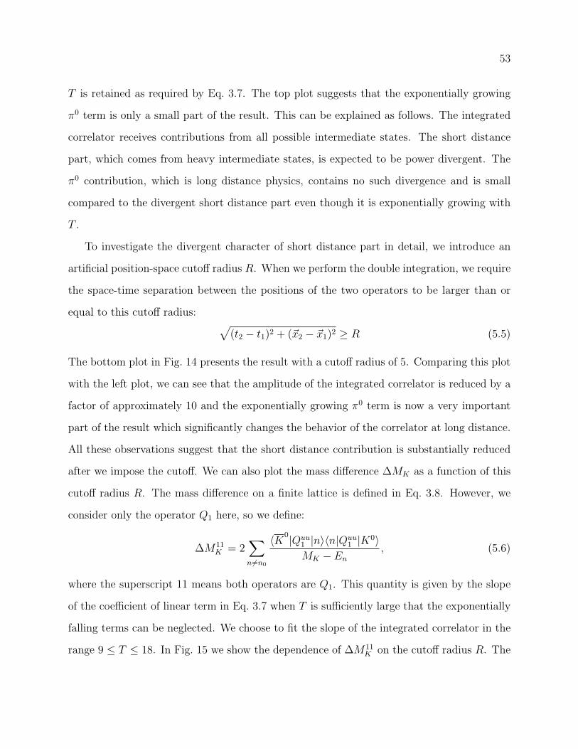
53
T is retained as required by Eq. 3.7. The top plot suggests that the exponentially growing
π0 term is only a small part of the result. This can be explained as follows. The integrated
correlator receives contributions from all possible intermediate states. The short distance
part, which comes from heavy intermediate states, is expected to be power divergent. The
π0 contribution, which is long distance physics, contains no such divergence and is small
compared to the divergent short distance part even though it is exponentially growing with
T .
To investigate the divergent character of short distance part in detail, we introduce an
artificial position-space cutoff radius R. When we perform the double integration, we require
the space-time separation between the positions of the two operators to be larger than or
equal to this cutoff radius:√
(t2 − t1)2 + (~x2 − ~x1)2 ≥ R (5.5)
The bottom plot in Fig. 14 presents the result with a cutoff radius of 5. Comparing this plot
with the left plot, we can see that the amplitude of the integrated correlator is reduced by a
factor of approximately 10 and the exponentially growing π0 term is now a very important
part of the result which significantly changes the behavior of the correlator at long distance.
All these observations suggest that the short distance contribution is substantially reduced
after we impose the cutoff. We can also plot the mass difference ∆MK as a function of this
cutoff radius R. The mass difference on a finite lattice is defined in Eq. 3.8. However, we
consider only the operator Q1 here, so we define:
∆M11K = 2
∑
n 6=n0
〈K0|Quu1 |n〉〈n|Quu
1 |K0〉MK − En
, (5.6)
where the superscript 11 means both operators are Q1. This quantity is given by the slope
of the coefficient of linear term in Eq. 3.7 when T is sufficiently large that the exponentially
falling terms can be neglected. We choose to fit the slope of the integrated correlator in the
range 9 ≤ T ≤ 18. In Fig. 15 we show the dependence of ∆M11K on the cutoff radius R. The
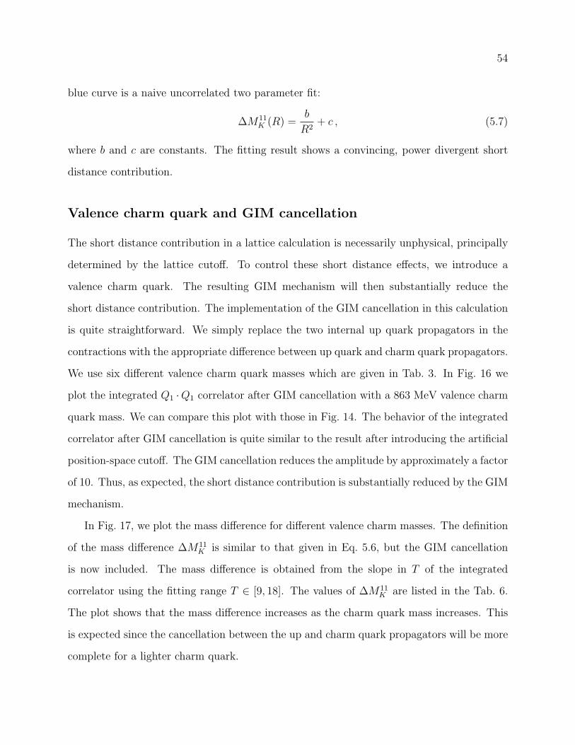
54
blue curve is a naive uncorrelated two parameter fit:
∆M11K (R) =
b
R2+ c , (5.7)
where b and c are constants. The fitting result shows a convincing, power divergent short
distance contribution.
Valence charm quark and GIM cancellation
The short distance contribution in a lattice calculation is necessarily unphysical, principally
determined by the lattice cutoff. To control these short distance effects, we introduce a
valence charm quark. The resulting GIM mechanism will then substantially reduce the
short distance contribution. The implementation of the GIM cancellation in this calculation
is quite straightforward. We simply replace the two internal up quark propagators in the
contractions with the appropriate difference between up quark and charm quark propagators.
We use six different valence charm quark masses which are given in Tab. 3. In Fig. 16 we
plot the integrated Q1 ·Q1 correlator after GIM cancellation with a 863 MeV valence charm
quark mass. We can compare this plot with those in Fig. 14. The behavior of the integrated
correlator after GIM cancellation is quite similar to the result after introducing the artificial
position-space cutoff. The GIM cancellation reduces the amplitude by approximately a factor
of 10. Thus, as expected, the short distance contribution is substantially reduced by the GIM
mechanism.
In Fig. 17, we plot the mass difference for different valence charm masses. The definition
of the mass difference ∆M11K is similar to that given in Eq. 5.6, but the GIM cancellation
is now included. The mass difference is obtained from the slope in T of the integrated
correlator using the fitting range T ∈ [9, 18]. The values of ∆M11K are listed in the Tab. 6.
The plot shows that the mass difference increases as the charm quark mass increases. This
is expected since the cancellation between the up and charm quark propagators will be more
complete for a lighter charm quark.
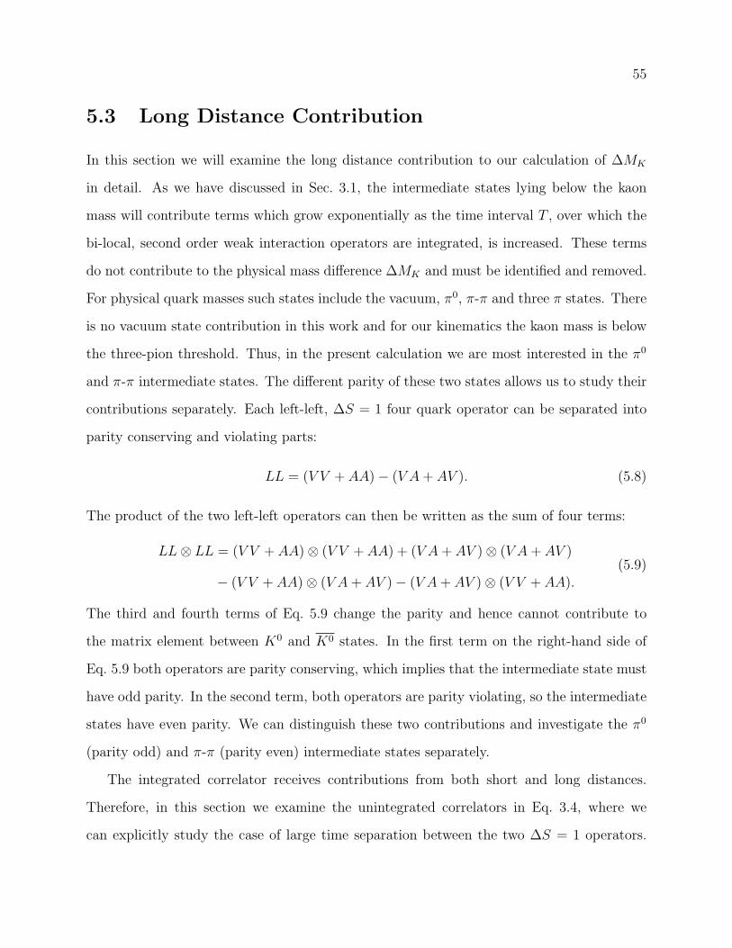
55
5.3 Long Distance Contribution
In this section we will examine the long distance contribution to our calculation of ∆MK
in detail. As we have discussed in Sec. 3.1, the intermediate states lying below the kaon
mass will contribute terms which grow exponentially as the time interval T , over which the
bi-local, second order weak interaction operators are integrated, is increased. These terms
do not contribute to the physical mass difference ∆MK and must be identified and removed.
For physical quark masses such states include the vacuum, π0, π-π and three π states. There
is no vacuum state contribution in this work and for our kinematics the kaon mass is below
the three-pion threshold. Thus, in the present calculation we are most interested in the π0
and π-π intermediate states. The different parity of these two states allows us to study their
contributions separately. Each left-left, ∆S = 1 four quark operator can be separated into
parity conserving and violating parts:
LL = (V V + AA)− (V A+ AV ). (5.8)
The product of the two left-left operators can then be written as the sum of four terms:
LL⊗ LL = (V V + AA)⊗ (V V + AA) + (V A+ AV )⊗ (V A+ AV )
− (V V + AA)⊗ (V A+ AV )− (V A+ AV )⊗ (V V + AA).(5.9)
The third and fourth terms of Eq. 5.9 change the parity and hence cannot contribute to
the matrix element between K0 and K0 states. In the first term on the right-hand side of
Eq. 5.9 both operators are parity conserving, which implies that the intermediate state must
have odd parity. In the second term, both operators are parity violating, so the intermediate
states have even parity. We can distinguish these two contributions and investigate the π0
(parity odd) and π-π (parity even) intermediate states separately.
The integrated correlator receives contributions from both short and long distances.
Therefore, in this section we examine the unintegrated correlators in Eq. 3.4, where we
can explicitly study the case of large time separation between the two ∆S = 1 operators.
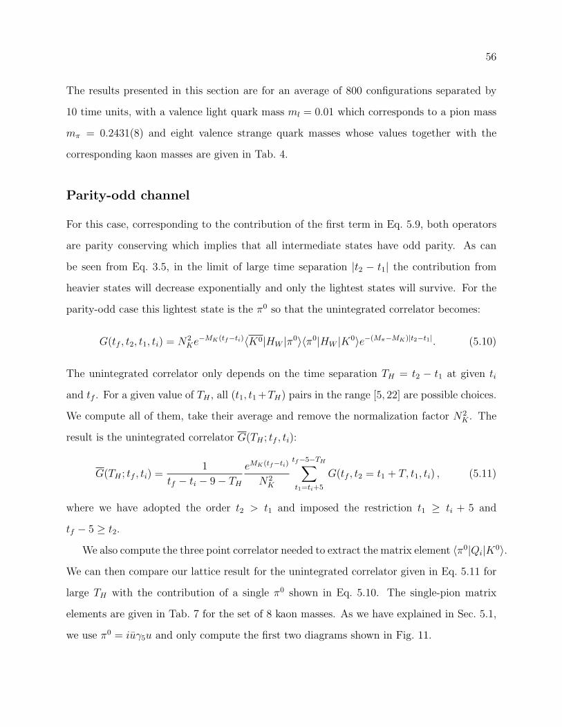
56
The results presented in this section are for an average of 800 configurations separated by
10 time units, with a valence light quark mass ml = 0.01 which corresponds to a pion mass
mπ = 0.2431(8) and eight valence strange quark masses whose values together with the
corresponding kaon masses are given in Tab. 4.
Parity-odd channel
For this case, corresponding to the contribution of the first term in Eq. 5.9, both operators
are parity conserving which implies that all intermediate states have odd parity. As can
be seen from Eq. 3.5, in the limit of large time separation |t2 − t1| the contribution from
heavier states will decrease exponentially and only the lightest states will survive. For the
parity-odd case this lightest state is the π0 so that the unintegrated correlator becomes:
G(tf , t2, t1, ti) = N2Ke
−MK(tf−ti)〈K0|HW |π0〉〈π0|HW |K0〉e−(Mπ−MK)|t2−t1|. (5.10)
The unintegrated correlator only depends on the time separation TH = t2 − t1 at given ti
and tf . For a given value of TH , all (t1, t1+TH) pairs in the range [5, 22] are possible choices.
We compute all of them, take their average and remove the normalization factor N2K . The
result is the unintegrated correlator G(TH ; tf , ti):
G(TH ; tf , ti) =1
tf − ti − 9− TH
eMK(tf−ti)
N2K
tf−5−TH∑
t1=ti+5
G(tf , t2 = t1 + T, t1, ti) , (5.11)
where we have adopted the order t2 > t1 and imposed the restriction t1 ≥ ti + 5 and
tf − 5 ≥ t2.
We also compute the three point correlator needed to extract the matrix element 〈π0|Qi|K0〉.
We can then compare our lattice result for the unintegrated correlator given in Eq. 5.11 for
large TH with the contribution of a single π0 shown in Eq. 5.10. The single-pion matrix
elements are given in Tab. 7 for the set of 8 kaon masses. As we have explained in Sec. 5.1,
we use π0 = iuγ5u and only compute the first two diagrams shown in Fig. 11.
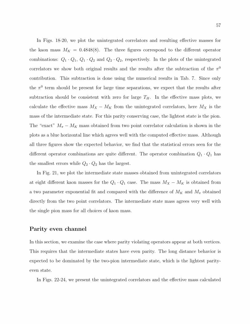
57
In Figs. 18-20, we plot the unintegrated correlators and resulting effective masses for
the kaon mass MK = 0.4848(8). The three figures correspond to the different operator
combinations: Q1 · Q1, Q1 · Q2 and Q2 · Q2, respectively. In the plots of the unintegrated
correlators we show both original results and the results after the subtraction of the π0
contribution. This subtraction is done using the numerical results in Tab. 7. Since only
the π0 term should be present for large time separations, we expect that the results after
subtraction should be consistent with zero for large TH . In the effective mass plots, we
calculate the effective mass MX − MK from the unintegrated correlators, here MX is the
mass of the intermediate state. For this parity conserving case, the lightest state is the pion.
The “exact” Mπ −MK mass obtained from two point correlator calculation is shown in the
plots as a blue horizontal line which agrees well with the computed effective mass. Although
all three figures show the expected behavior, we find that the statistical errors seen for the
different operator combinations are quite different. The operator combination Q1 · Q1 has
the smallest errors while Q2 ·Q2 has the largest.
In Fig. 21, we plot the intermediate state masses obtained from unintegrated correlators
at eight different kaon masses for the Q1 · Q1 case. The mass MX − MK is obtained from
a two parameter exponential fit and compared with the difference of MK and Mπ obtained
directly from the two point correlators. The intermediate state mass agrees very well with
the single pion mass for all choices of kaon mass.
Parity even channel
In this section, we examine the case where parity violating operators appear at both vertices.
This requires that the intermediate states have even parity. The long distance behavior is
expected to be dominated by the two-pion intermediate state, which is the lightest parity-
even state.
In Figs. 22-24, we present the unintegrated correlators and the effective mass calculated
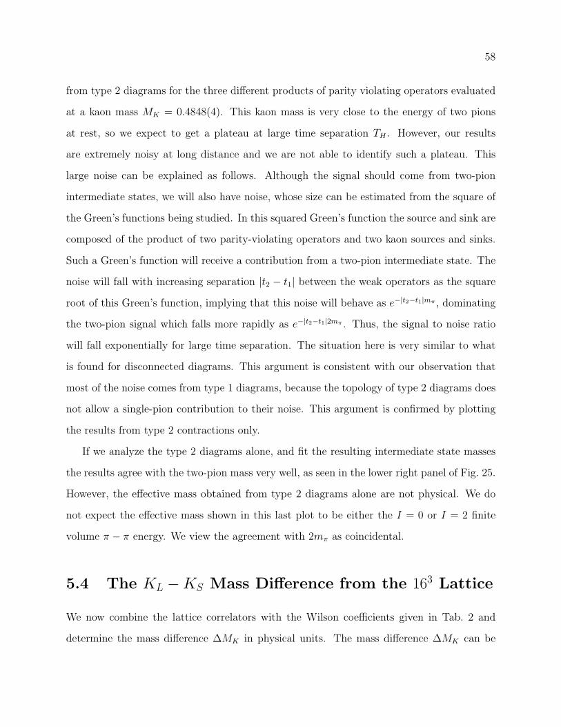
58
from type 2 diagrams for the three different products of parity violating operators evaluated
at a kaon mass MK = 0.4848(4). This kaon mass is very close to the energy of two pions
at rest, so we expect to get a plateau at large time separation TH . However, our results
are extremely noisy at long distance and we are not able to identify such a plateau. This
large noise can be explained as follows. Although the signal should come from two-pion
intermediate states, we will also have noise, whose size can be estimated from the square of
the Green’s functions being studied. In this squared Green’s function the source and sink are
composed of the product of two parity-violating operators and two kaon sources and sinks.
Such a Green’s function will receive a contribution from a two-pion intermediate state. The
noise will fall with increasing separation |t2 − t1| between the weak operators as the square
root of this Green’s function, implying that this noise will behave as e−|t2−t1|mπ , dominating
the two-pion signal which falls more rapidly as e−|t2−t1|2mπ . Thus, the signal to noise ratio
will fall exponentially for large time separation. The situation here is very similar to what
is found for disconnected diagrams. This argument is consistent with our observation that
most of the noise comes from type 1 diagrams, because the topology of type 2 diagrams does
not allow a single-pion contribution to their noise. This argument is confirmed by plotting
the results from type 2 contractions only.
If we analyze the type 2 diagrams alone, and fit the resulting intermediate state masses
the results agree with the two-pion mass very well, as seen in the lower right panel of Fig. 25.
However, the effective mass obtained from type 2 diagrams alone are not physical. We do
not expect the effective mass shown in this last plot to be either the I = 0 or I = 2 finite
volume π − π energy. We view the agreement with 2mπ as coincidental.
5.4 The KL −KS Mass Difference from the 163 Lattice
We now combine the lattice correlators with the Wilson coefficients given in Tab. 2 and
determine the mass difference ∆MK in physical units. The mass difference ∆MK can be
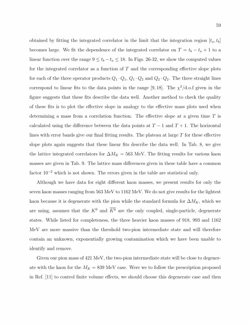
59
obtained by fitting the integrated correlator in the limit that the integration region [ta, tb]
becomes large. We fit the dependence of the integrated correlator on T = tb − ta + 1 to a
linear function over the range 9 ≤ tb− ta ≤ 18. In Figs. 26-32, we show the computed values
for the integrated correlator as a function of T and the corresponding effective slope plots
for each of the three operator products Q1 ·Q1, Q1 ·Q2 and Q2 ·Q2. The three straight lines
correspond to linear fits to the data points in the range [9, 18]. The χ2/d.o.f given in the
figure suggests that these fits describe the data well. Another method to check the quality
of these fits is to plot the effective slope in analogy to the effective mass plots used when
determining a mass from a correlation function. The effective slope at a given time T is
calculated using the difference between the data points at T − 1 and T + 1. The horizontal
lines with error bands give our final fitting results. The plateau at large T for these effective
slope plots again suggests that these linear fits describe the data well. In Tab. 8, we give
the lattice integrated correlators for ∆MK = 563 MeV. The fitting results for various kaon
masses are given in Tab. 9. The lattice mass differences given in these table have a common
factor 10−2 which is not shown. The errors given in the table are statistical only.
Although we have data for eight different kaon masses, we present results for only the
seven kaon masses ranging from 563 MeV to 1162 MeV. We do not give results for the lightest
kaon because it is degenerate with the pion while the standard formula for ∆MK , which we
are using, assumes that the K0 and K0 are the only coupled, single-particle, degenerate
states. While listed for completeness, the three heavier kaon masses of 918, 993 and 1162
MeV are more massive than the threshold two-pion intermediate state and will therefore
contain an unknown, exponentially growing contamination which we have been unable to
identify and remove.
Given our pion mass of 421 MeV, the two-pion intermediate state will be close to degener-
ate with the kaon for the MK = 839 MeV case. Were we to follow the prescription proposed
in Ref. [11] to control finite volume effects, we should choose this degenerate case and then

60
remove completely the contribution of the degenerate, two-pion intermediate state, which
should appear in the integrated correlator with the time dependence (tb − ta)2. However, as
explained earlier, we are not able to identify the two-pion intermediate state within errors.
This implies that the approximately on-shell, two-pion intermediate state contributes only a
small part to the mass difference in our calculation and should have a small effect, at least
on the results for 563 MeV ≤ MK ≤ 834 MeV.
5.5 Comparison with NLO Perturbative Calculation
A direct comparison between our results and the experimental value of ∆MK has limited
value because our kaon and pion masses are far from physical and we have not included
all diagrams. However, we can learn something about the degree to which the present
perturbative calculations describe ∆MK for our unphysical kinematics by comparing our
result with that obtained perturbatively by evaluating the perturbative formula at the kaon
and pion masses used in our present calculation. While there are now results for ∆MK
computed at NNLO given in Ref. [8], complete expressions for the results are not given in
that brief letter. Therefore, we choose to compare with the NLO result of Herrlich and
Nierste [25] for which complete information is available in published form. Since the full
results at NLO and NNLO orders differ by 36% at the physical point, the agreement with
our result should be only approximate and this use of the NLO result adequate for our
purpose. This comparison with NLO perturbation theory may also lessen the significance of
our omission of disconnected diagrams, which do not appear at NLO. We will compare this
NLO result, evaluated at our kinematics, with our lattice calculation carried out using 600
configurations at the unitary quark masses ml = 0.01 and ms = 0.032 (Mπ = 421 MeV and
MK = 563 MeV) for a series of valence charm quark masses.

61
The mass difference in the perturbative calculation is given by:
∆MK =G2
F
6π2f 2KBKMK(λ− λ3
2)2η1(µc,mc(µc))m
2c(µc), (5.12)
which can be obtained, for example, from Eq. (12.1) in Ref. [13]. Here λ is the sine of the
Cabibbo angle, one of the four Wolfenstein parameters entering the CKM matrix, µc is the
scale at which the four-flavor theory is matched to that with three flavors and the kaon
decay constant fK is defined using conventions which make its physical value equal to 155
MeV. The two non-perturbative parameters, the kaon decay constant fK and the kaon bag
parameter BK , evaluated in the renormalization group invariant (RGI) scheme, can also be
computed for the unphysical values of ml and ms listed above. For the present calculation
we find it convenient to directly compute the matrix element of the left-left operator:
〈OLL〉 = 〈K0|(sd)V−A(sd)V−A|K0〉, (5.13)
obtaining the value 0.00462(5) for ml = 0.01 and ms = 0.032. Here we use non-relativistic
normalization for the kaon states: 〈K(~p)|K(~p ′)〉 = δ3(~p − ~p ′). This lattice result can be
converted to the RGI scheme by multiplying by the factor:
ZRGIV V+AA = ZRGI
BKZ2
A, (5.14)
where ZRGIBK = 1.27 and ZA = 0.7161 are taken from Ref. [26].
The expression for the mass difference then becomes:
∆MK =G2
F
8π2ZRGI
BKZ2
A〈OLL〉(λ− λ3
2)2η1 (µc,mc(µc))m
2c(µc). (5.15)
Here the factors ZRGIBK
Z2A〈OLL〉 are lattice quantities determined for the kinematics studied
here while η1 is determined from the NLO perturbation theory calculation of Ref. [25],
summarized in Ref. [13]. Specifically, Eq. (5.15) corresponds to the term in Eq. (12.1) of
Ref. [13] containing η1. Note, the two right-most factors in Eq. (12.1) do not appear in our
Eq. (5.15) since they have been incorporated in BK , changing it to the RGI scheme. We
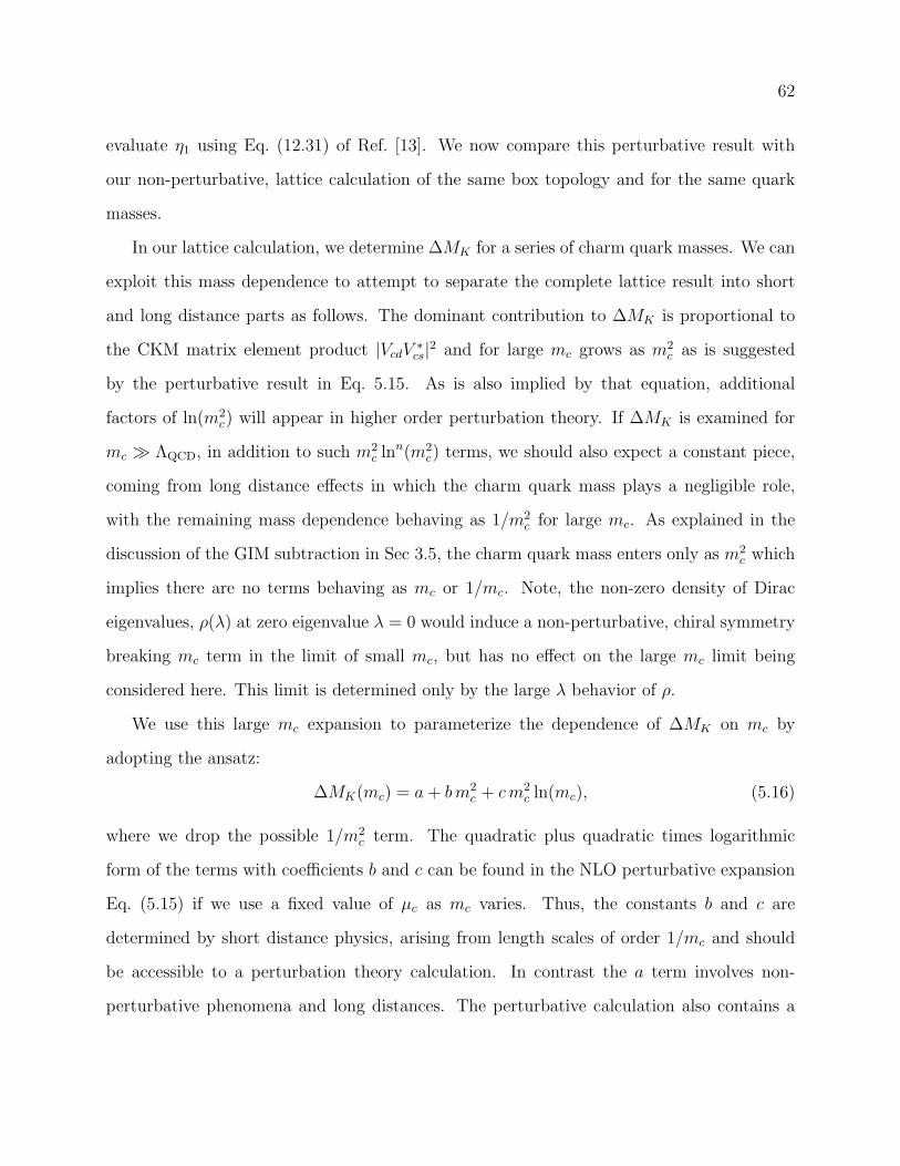
62
evaluate η1 using Eq. (12.31) of Ref. [13]. We now compare this perturbative result with
our non-perturbative, lattice calculation of the same box topology and for the same quark
masses.
In our lattice calculation, we determine ∆MK for a series of charm quark masses. We can
exploit this mass dependence to attempt to separate the complete lattice result into short
and long distance parts as follows. The dominant contribution to ∆MK is proportional to
the CKM matrix element product |VcdV∗cs|2 and for large mc grows as m2
c as is suggested
by the perturbative result in Eq. 5.15. As is also implied by that equation, additional
factors of ln(m2c) will appear in higher order perturbation theory. If ∆MK is examined for
mc ≫ ΛQCD, in addition to such m2c ln
n(m2c) terms, we should also expect a constant piece,
coming from long distance effects in which the charm quark mass plays a negligible role,
with the remaining mass dependence behaving as 1/m2c for large mc. As explained in the
discussion of the GIM subtraction in Sec 3.5, the charm quark mass enters only as m2c which
implies there are no terms behaving as mc or 1/mc. Note, the non-zero density of Dirac
eigenvalues, ρ(λ) at zero eigenvalue λ = 0 would induce a non-perturbative, chiral symmetry
breaking mc term in the limit of small mc, but has no effect on the large mc limit being
considered here. This limit is determined only by the large λ behavior of ρ.
We use this large mc expansion to parameterize the dependence of ∆MK on mc by
adopting the ansatz:
∆MK(mc) = a+ bm2c + cm2
c ln(mc), (5.16)
where we drop the possible 1/m2c term. The quadratic plus quadratic times logarithmic
form of the terms with coefficients b and c can be found in the NLO perturbative expansion
Eq. (5.15) if we use a fixed value of µc as mc varies. Thus, the constants b and c are
determined by short distance physics, arising from length scales of order 1/mc and should
be accessible to a perturbation theory calculation. In contrast the a term involves non-
perturbative phenomena and long distances. The perturbative calculation also contains a
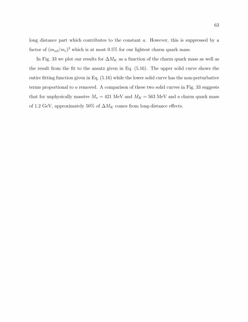
63
long distance part which contributes to the constant a. However, this is suppressed by a
factor of (mud/mc)2 which is at most 0.5% for our lightest charm quark mass.
In Fig. 33 we plot our results for ∆MK as a function of the charm quark mass as well as
the result from the fit to the ansatz given in Eq. (5.16). The upper solid curve shows the
entire fitting function given in Eq. (5.16) while the lower solid curve has the non-perturbative
terms proportional to a removed. A comparison of these two solid curves in Fig. 33 suggests
that for unphysically massive Mπ = 421 MeV and MK = 563 MeV and a charm quark mass
of 1.2 GeV, approximately 50% of ∆MK comes from long-distance effects.
Chapter 6
Results from the 243 × 64× 16 Lattice
In this chapter, we will give the results from the 243 × 64× 16 lattice ensemble. Section. 6.1
describes the details of the simulation. Section. 6.2 gives the mass difference calculated on
this lattice. In Section. 6.3, we discuss the contribution to the mass difference from the
different diagrams. In Section. 6.4, we discuss the effects of the scalar and pseudo-scalar
operators in our calculation.
6.1 Simulation Details
The 243 lattice ensemble is similar to the 163 lattice ensemble described in the last chapter
except for a larger volume and a lighter pion mass. The sea light and strange quark masses
are ml = 0.005 and ms = 0.04 respectively, corresponding to a 330 MeV pion mass and a
575 MeV kaon mass. A valence charm quark mass mc = 0.363 is used to implement GIM
cancellation, corresponding tomMSc (2GeV) = 949. We use 800 configurations, each separated
by 10 time units.
We will refer to Fig. 4 to explain the setup of this calculation. All the diagrams are
included in this unitary calculation. For the kaon sources, we continue to use Coulomb-
gauge-fixed wall sources. However, unlike the 163 calculation, the locations of the two kaons
64
65
are not fixed. All the diagrams are averaged over all time translations to increase statistics.
We also vary the separation between the two kaons in this calculation. This separation
should be sufficient large so that the interaction range is large enough to extract the mass
difference. Since we are not using periodic plus anti-periodic boundary condition here, this
separation should not be too large so that we don’t need to worry about the around-the-
world effects. In our calculation, we vary this separation from 24 lattice units to 31 lattice
units. The separation between the kaon sources and the effective Hamiltonian densities
should be sufficiently large to suppress the contribution from the excited kaons. We choose
this separation to be equal or larger than 6 lattice units in our calculation.
The evaluation of the four point correlators are explained in Section. 4.4. For type 1
and type 2 diagrams, 64 propagators are computed using a point source on each of the 64
time slices. For type 3 and type 4 diagrams, we use 64 random wall source propagators to
construct the quark loops. In order to reduce the noise coming from the random numbers,
we use 6 sets of random sources for each time slice, color and spin. For the light quark
propagators, which make up the most expensive part of this calculation, we calculate the
lowest 300 eigenvectors of the Dirac operator using the Lanczos method and get a factor of
8 speed up by using mix precision CG solver with low mode deflation. The parameters for
the Lanczos algorithm are given in Tab. 11. For the strange and charm quarks, we use the
mix precision CG solver. We use a 10−5 stopping condition for the inner single precision CG
solvers and use a 10−8 stopping condition for the outer CG solvers.
6.2 The KL −KS Mass Difference from the 243 Lattice
In this unitary calculation, the integrated correlators will receive exponentially increasing
contributions from both the π0 and vacuum intermediate states. We evaluate the matrix
element 〈π0|HW |K0〉 and subtract the single pion exponentially increasing term explicitly
from Eq.3.7. For the vacuum state, we add a pseudo-scalar density sγ5d to the weak Hamil-
66
tonian to eliminate the matrix element 〈0|HW + c2sγ5d|K0〉. The details of this subtraction
has been discussed in Section. 3.1. We also perform a subtraction for the exponentially
decreasing term from η state. We have a 624 MeV η meson mass in our calculation, which
is slightly heavier than the 575 MeV kaon mass. The exponential term from η state will
decreasing slowly and may contaminate the linear behavior at large T . So we subtract this
term by using the 〈η|HW |K0〉 matrix element calculated from three point correlators. This
has a less than 10% effect on the final result. The (ππ)I=0 state energy is 629 MeV for our
kinematics [27]. The exponential term from (ππ)I=0 state will also be decreasing slowly. We
are not able to subtract this term since we don’t have the date for the K → (ππ)I=0 matrix
element. This is a source of the systematic errors in our calculation. However, the χ2/d.o.f
values for our linear fits suggest this term gives small contribution.
In Fig. 34, we show the the integrated correlators and the corresponding effective mass
plots for the case in which the kaon sources are separated by 31 lattice units. The three curves
correspond to the three different operator combinations: Q1 ·Q1, Q1 ·Q2 and Q2 ·Q2. The
numbers are bare lattice results without any Wilson coefficients or renormalization factors.
All the exponentially increasing terms have been removed from the correlators, so we expect
a linear behavior for sufficiently large T . When T becomes too large, the errors explode as
should be expected since the disconnected diagrams have an exponentially decreasing signal-
to-noise ratio. The straight lines correspond to linear fits to the data points in the range
[7, 20]. The χ2/d.o.f given in the figure suggest that these fits describe the data well. The
effective slope is calculated using a method different from the method in Section. 5.4. At a
given time T , the effective slope is calculated using a correlated linear fit to three data points
at T − 1, T and T + 1. For each operator combination we get good plateaus starting from
T = 7. In Tab. 12, we give the lattice integrated correlators without any Wilson coefficients
for the three operator products. The fitting results for the mass differences are given in
Tab. 13. We give both the bare lattice numbers without Wilson coefficients and the physical
67
values with Wilson coefficients.
We have the results for the integrated correlators for two kaon separation ∆KK from
24 lattice units to 31 lattice units. In Tab. 14, we give the fitting results from difference
choices of ∆KK. We choose a minimum fitting time Tmin = 7 for all the fits. The fitting
results from different choices of ∆KK have similar central values and error-bars. The error-
weighted-average given in the last row suggest that combining these results dose not improve
the errors. Hence we conclude that these results are highly correlated and we will not benefit
from a combined analysis. So we will focus on the ∆KK = 31 case in the following analysis.
We have also tried different fitting ranges to make sure that our results do not depend
sensitively on these choices. We varied two parameters: the lower limit on the linear fitting
range Tmin and the minimum separation between the kaon sources and weak Hamiltonians
∆min. We first fixed ∆K = 6 and varied Tmin from 7 to 9. The results are given in Table. 15.
While the central value of the fitting results are quite stable, the errors are sensitive to
the choice of Tmin, which is caused by the exponentially decreasing signal-to-noise ratio of
disconnected diagrams. We vary ∆min to check whether or not there are contaminations
from excited kaon states. We give the results in Table. 16 for fixed Tmin = 7 but with ∆min
varying from 6 to 8. Both the central values and the errors are very stable, suggesting that
a separation of 6 is large enough to suppress excited kaon states.
6.3 Contributions from Different Diagrams
In our 163 calculation, only the first two types of diagrams were included in the calculation.
We can now determine the accuracy of this approximation by calculating the contribution
from each type of diagrams separately. The subtraction of π0 exponentially increasing term
will become more complicated if we analyze different types of diagrams separately. We
perform a subtraction for each type of diagrams separately following a procedure similar
to our previous work [?]. For the vacuum state, we don’t have such complication since the
68
vacuum state contribution only comes from type 4 diagrams. Adding a sγ5d term will remove
the exponentially increasing term for type 4 diagrams and will not cause any other problem.
We perform a subtraction for the slow decaying term from η state in the full analysis. In
a separate analysis, we are not able to separate the η contribution into different types of
diagram in a reasonable way. So we don’t perform any subtraction for η state here.
In Fig. 35-38, we give the integrated correlators and the corresponding diagrams for the
four different types of diagrams. For type 1 and type 4 diagrams, we obtain good linear
behavior at the large T range and the χ2/d.o.f are also close to 1. Although the integrated
correlators for type 2 diagrams appears to be very linear, the χ2/d.o.f values are very large.
For type 3 diagrams, the effective slope plots suggest that there are some non-linear behavior
at large T . This unexpected behavior can be caused by excited kaon states. We can increase
∆min to suppress the contribution from excited kaon states. In Fig. 39-42, we give the results
for the choice of ∆min = 8. The effective slopes from the type 3 diagrams do become better.
The large χ2/d.o.f for type 2 diagrams improve but are still not perfect. We should keep in
mind that the results from each individual type of diagram are not physical and we are not
guaranteed to obtain a linear behavior for each type of diagram separately.
In Tab. 17, we give ∆MK from different types of diagrams. We choose ∆min = 8 for
all the fittings. If we focus on the final results for ∆MK , the contribution from type 1 and
type 3 diagrams are relatively small. There is a large cancellation between the disconnected
(type 4) diagrams and other type of diagrams. The mass difference is reduced by almost
a factor of two after the inclusion of the disconnected diagrams. This is a surprisingly
large failure of the“OZI suppression” [21, 22, 23], naively expected for these disconnected
diagrams. Although this result may be surprising, we should always keep in mind that the
mass difference from individual types of diagrams is not a physical quantity and we should
not put too much emphasis on these results.
69
6.4 Effects of Scalar and Pseudoscalar Operators
In this calculation, we remove the π0 exponentially increasing term explicitly and add a
pseudoscalar density to the Hamiltonian to eliminate the vacuum states. We can also add
a scalar density to the Hamiltonian to eliminate the π0 state so that we do not need to
perform the subtraction. In Section. 3.1, we claim that adding these operators will not
change the final results. We will examine the effects of the scalar and the pseudo-scalar
operators numerically in this section.
We can rewrite the Hamiltonian in Eq. 3.11 as:
H ′W = HW + cscπsd+ cpcvacsγ
5d, (6.1)
where cπ and cvac are defined in Eq. 3.15 and cs and cp are dimensionless numbers. In Sec. 6.2,
we choose cs = 0 and cp = 1. If we choose other value for cs and cp, the resulting exponentially
increasing terms can be determined and subtracted by using the matrix elements 〈π0|H ′W |K0〉
and 〈0|H ′W |K0〉. In the next few paragraphs, we will vary cs and cp and determine whether
or not the mass difference will depend on the choice of these values.
We will first vary the value of cs while the value of cp is fixed to 1. Generally, the mass
differences can have both linear and quadratic dependence on cs. The linear dependence
comes from the operator products Qi · sd and the quadratic dependence comes from the
operator product sd · sd. In Fig. 43, we give the integrated correlator for these operator
products. We expect these plots have a zero slope at large T range since sd operator should
not contribute to the mass difference. The results are within our expectation.
In Figure. 47, the mass differences are plotted for cs value from -1 to 1. The plots for the
integrated correlators and the corresponding effective slope plots for cs = 1 and cs = −1 are
given in Figs. 44-45. We can also tune the value of cs to eliminate the η intermediate state.
The corresponding results are given in Fig.46. In Tab. 18, we give the mass differences for
various choices of cs. We conclude that the mass differences are independent of the choices
70
of the value of cs.
Next we will vary the value of cp while the value of cs is fixed to 0. The first difficulty
here is the subtraction of the exponentially increasing term coming from the vacuum state
when cp 6= 1. This term is two orders of magnitude larger than the linear term if we choose
cp = 0. For the subtraction of the π0 exponentially increasing term, we use the formula given
in Eq. 3.7. However, this formula uses a second order integration instead of a second order
sum. The more precise formula for the vacuum exponential term is given by:
N2Ke
−MK(tf−ti)〈K0|HW |0〉〈0|HW |K0〉 eMKT − 1
4Sinh2(MK/2). (6.2)
Comparing with Eq. 3.7, the M2K in the denominator is changed to 4sinh2(MK/2), which is
a O(a2) correction. For MK = 0.3325, there is a 1% differnce between these two formula.
Since we are trying to subtract a term which is two orders of magnitude larger than the
signal, this is a necessary correction here.
In the first plot in Fig. 48, we give the integrated correlator for cp = 0, cs = 1 and ∆min =
6. We can see that the integrated correlators at large T are not linear. A possible cause of
this behavior is a contribution from excited kaon states. Our signal is supposed to behave as
e−MK(tf−ti). The exponentially increasing vacuum term receives its largest contribution when
the vacuum travels the entire interaction range T and behaves like e−MK(tf−ti−T ). This is
emKT larger than the signal and needs to be removed. For the cp = 1 case, the vacuum state
will not couple to kaon ground state and the contribution from the excited kaon state K∗
behaves as e−MK∗ (tf−ti−T ). We have repeated the calculation for different values of tf − ti−T
and the results are consistent. So the excited kaon state is likely not important if cp = 1.
However, if we consider cp = 0, we can have a kaon on onside and an excited kaon on the
other side. The excited kaon contribution will behave like e−MK(tf−ti−T )/2e−MK∗ (tf−ti−T )/2,
which for large T grows exponentially larger than the signal which behaves as e−mK(tf−ti)
and may obscure the expected linear large T behavior.
In the second plot in Fig. 48, we increase ∆min from 6 to 10. Although the integrated
71
correlator appears to be better, the results are actually not changed much if we just compare
the integrated correlator in the time interval [7, 12]. This is confirmed by the fitting results
given in Tab. 19. The results we get for two ∆min values are consistent and are quite different
from the mass difference from cp = 1 data. This difference is likely due to some uncontrolled
systematic effects introduced when we try to remove the exponentially increasing term from
the cp = 0 data. In Tab. 20, we can see that the mass difference comes from the vacuum
state when is 10 times larger than the final mass difference. This large contribution is
mostly non-physical and coming from the mixing between the Hamiltonian and the sγ5d
operator. If we can control every aspect of this calculation, this large contribution will be
canceled by other unphysical contributions and the final results should be consistent with
cp = 1 results. However, it seems that we can only remove the vacuum contribution to 10%
precision and hence the mass difference for cp = 0 case is completely different from the cp = 1
results. In Fig. 49, we give the mass difference for different values of cp while cs is fixed to
1. The mass difference will change rapidly when cp deviates from 1. ∆M11’s dependence
on cp is mild while ∆M22’s dependence is the strongest among the three operator products.
This is consistent with the fact that the contribution to ∆M22 from the vacuum state is 30
times larger than the vacuum contribution to ∆M11. So we conclude that there are some
uncontrolled systematic effect from the subtraction of vacuum states and we are not able to
obtain a reliable value for ∆MK if cp is too far away from 1. If we choose cp = 1, there will
be no contribution from vacuum states and we will not have this trouble.

Chapter 7
Conclusions
In the previous two chapters, we showed detailed results for ∆MK from a 163 × 32 × 16
lattice ensemble and a 243 × 64× 16 lattice ensemble. These calculations are all done with
a heavy pion mass and with a quenched charm quark on a relatively coarse lattice. We also
neglect the type 3 and 4 diagrams in the 163 lattice calculation. However, as a pioneering
calculation on this difficult problem with four-point correlators and disconnected diagrams,
our results have shown the success for application of the lattice QCD as a first-principal
method to compute a second-order weak processes.
In the 243 full calculation, we compute ∆MK for a case of unphysical kinematics with
pion, kaon and charmed quark masses of 330, 575 and 949 MeV respectively, each quite
different from their physical values of 135, 495 and 1100 MeV. Our results is:
∆MK = 3.19(41)(96)× 10−12MeV. (7.1)
Here the first error is statistical and the second an estimate of largest systematic error, the
discretization error which results from including a 949 MeV charm quark in a calculation
using an inverse lattice spacing 1/a = 1.73 GeV. This 30% estimate for the discretization
error can be obtained either by simple power counting, (mca)2 = 30%, or from the failure of
the calculated energy of the ηc meson to satisfy the relativistic dispersion relation. We find
72

73
(E2(p) −m2)/p2 = 0.740(3) instead of 1.0 when evaluated at p = 2π/L. Our result agrees
well with the experimental value of 3.483(6)× 10−12 MeV. However, since we are not using
physical kinematics, this agreement could be easily fortuitous.
One further potential difficulty which should be discussed associated with our inclusion
of a heavy charm quark is a phenomena particular to the domain wall fermion formalism.
When the input lattice quark mass,mf , becomes large, about 0.4 or larger in lattice units, the
eigenvalues of the physical, 4-dimensional modes become as large as the smallest eigenvalues
of unphysical, 5-dimensional modes [28, 29]. These 5-dimensional modes could add a further,
unphysical contribution to the GIM cancellation. We have examined the propagator for the
ηc state and determined that our value of mf = 0.363 lies slightly below the threshold at
which there is significant coupling to these bulk, 5-dimensional states.
This is illustrated in Fig. 50, where we show fqq as a function of mf . The quanity
fqq is the product of the pseudoscalar decay constant and the normalization factor for the
gauge fixed wall source. Here one sees a monotonic increase in fqq as mf increases up to a
value of mf ≈ 0.4, above which fqq turns over and decreases with increasing mf , suggesting
the appearance of propagating 5-dimensional modes, which necessarily have a substantially
reduced coupling to operators with support on the 4-dimensional s = 0 and s = Ls−1 walls.
A significant contribution from such unphysical, 5-dimension modes would add further lattice
artifacts to the GIM cancellation that controls the largest component of ∆MK . One of the
benefits of carrying out future calculations at smaller lattice spacing will be the further
reduction of the possibility of such contributions.
The disconnected diagrams contribute a large amount to our result for ∆MK . This
is a surprising result and suggests the failure of “OZI suppression” in the KL − KS mass
difference. The OZI rule argues that the disconnect diagrams are connected by hard gluons
and hence suppressed by a small gauge field coupling constant. However, there is no strict
theoretical basis for this rule. We view our result as strong evidence that the OZI rule is not
74
solid and may be unreliable in some cases.
To perform a calculation with physical kinematics and controlled systematic errors, two
difficulties must be overcome. First, we need to perform the calculation on a four-flavor lat-
tice ensemble with two or more, smaller lattice spacings. This would remove the difficult-to-
estimate error associated with quenching the charm quark and allow the O(m2ca
2) discretiza-
tion errors to be removed. Second, we must perform a finite volume correction associated
with π − π re-scattering which will be needed for physical kinematics, when the two-pion
threshold lies below the kaon mass. In this case, ∆MK in infinite volume contains the prin-
cipal part of the integral over the two-pion relative momentum, which can be substantially
different from a finite-volume momentum sum. A generalization of the Lellouch-Luscher
method has been devised to correct this potentially large finite volume effect [11] and a more
general method has been proposed in Ref. [30].
Similar techniques can be used to determine the long distance contribution to ǫK . How-
ever, the calculation of ǫK involves two additional complexities described in Appendix A
of Ref. [31]. First, we must introduce new QCD penguin operators representing top quark
effects. Second, an overall, logarithmic divergence must be removed from the lattice cal-
culation using non-perturbative methods. In summary, a full calculation of ∆MK and ǫK ,
including their long distance contributions, should be accessible to lattice QCD with con-
trolled systematic errors within a few years, substantially increasing the importance of these
quantities in the search for new phenomena beyond the standard model.
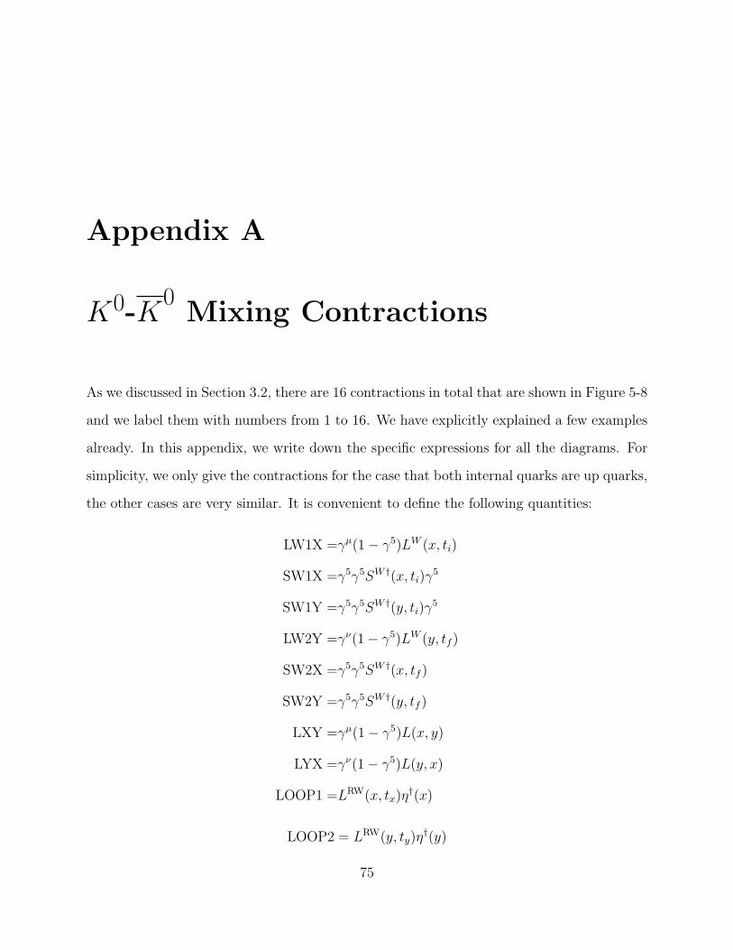
Appendix A
K0-K0Mixing Contractions
As we discussed in Section 3.2, there are 16 contractions in total that are shown in Figure 5-8
and we label them with numbers from 1 to 16. We have explicitly explained a few examples
already. In this appendix, we write down the specific expressions for all the diagrams. For
simplicity, we only give the contractions for the case that both internal quarks are up quarks,
the other cases are very similar. It is convenient to define the following quantities:
LW1X =γµ(1− γ5)LW (x, ti)
SW1X =γ5γ5SW †(x, ti)γ5
SW1Y =γ5γ5SW †(y, ti)γ5
LW2Y =γν(1− γ5)LW (y, tf )
SW2X =γ5γ5SW †(x, tf )
SW2Y =γ5γ5SW †(y, tf )
LXY =γµ(1− γ5)L(x, y)
LYX =γν(1− γ5)L(y, x)
LOOP1 =LRW(x, tx)η†(x)
LOOP2 = LRW(y, ty)η†(y)
75
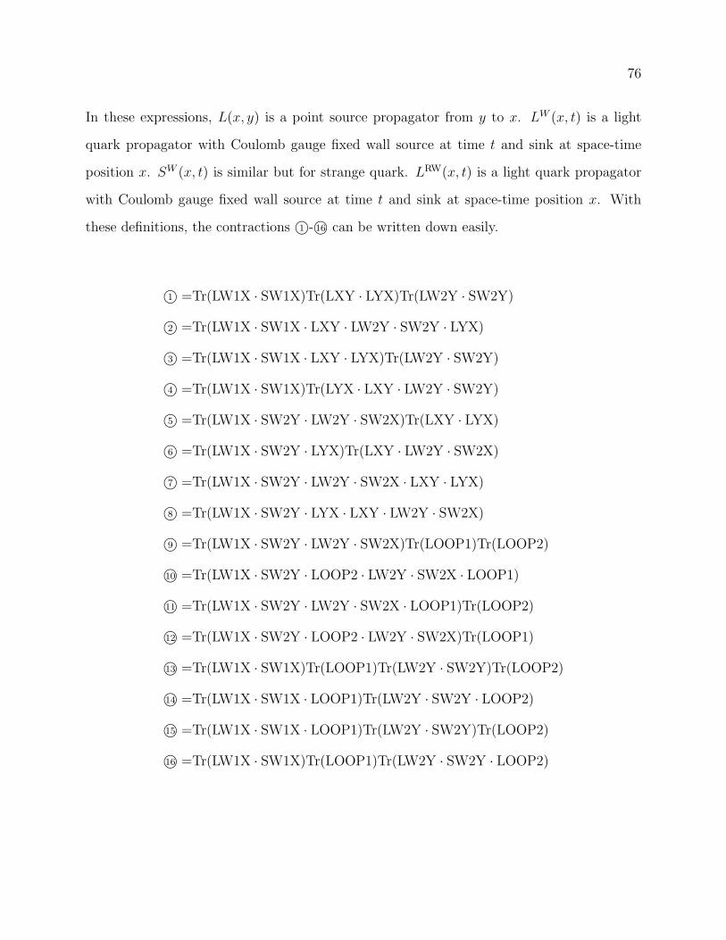
76
In these expressions, L(x, y) is a point source propagator from y to x. LW (x, t) is a light
quark propagator with Coulomb gauge fixed wall source at time t and sink at space-time
position x. SW (x, t) is similar but for strange quark. LRW(x, t) is a light quark propagator
with Coulomb gauge fixed wall source at time t and sink at space-time position x. With
these definitions, the contractions 1©- 16© can be written down easily.
1© =Tr(LW1X · SW1X)Tr(LXY · LYX)Tr(LW2Y · SW2Y)
2© =Tr(LW1X · SW1X · LXY · LW2Y · SW2Y · LYX)
3© =Tr(LW1X · SW1X · LXY · LYX)Tr(LW2Y · SW2Y)
4© =Tr(LW1X · SW1X)Tr(LYX · LXY · LW2Y · SW2Y)
5© =Tr(LW1X · SW2Y · LW2Y · SW2X)Tr(LXY · LYX)
6© =Tr(LW1X · SW2Y · LYX)Tr(LXY · LW2Y · SW2X)
7© =Tr(LW1X · SW2Y · LW2Y · SW2X · LXY · LYX)
8© =Tr(LW1X · SW2Y · LYX · LXY · LW2Y · SW2X)
9© =Tr(LW1X · SW2Y · LW2Y · SW2X)Tr(LOOP1)Tr(LOOP2)
10© =Tr(LW1X · SW2Y · LOOP2 · LW2Y · SW2X · LOOP1)
11© =Tr(LW1X · SW2Y · LW2Y · SW2X · LOOP1)Tr(LOOP2)
12© =Tr(LW1X · SW2Y · LOOP2 · LW2Y · SW2X)Tr(LOOP1)
13© =Tr(LW1X · SW1X)Tr(LOOP1)Tr(LW2Y · SW2Y)Tr(LOOP2)
14© =Tr(LW1X · SW1X · LOOP1)Tr(LW2Y · SW2Y · LOOP2)
15© =Tr(LW1X · SW1X · LOOP1)Tr(LW2Y · SW2Y)Tr(LOOP2)
16© =Tr(LW1X · SW1X)Tr(LOOP1)Tr(LW2Y · SW2Y · LOOP2)
Bibliography
[1] A. Stathopoulos and K. Orginos, SIAM J.Sci.Comput. 32, 439 (2010), 0707.0131.
[2] Q. Liu (2011), 1110.2143.
[3] R. Arthur (2012), Ph.D. thesis, University of Edinburgh, unpublished.
[4] K. Nakamura et al. (Particle Data Group), J.Phys.G G37, 075021 (2010).
[5] R. Mohapatra, J. S. Rao, and R. Marshak, Phys.Rev. 171, 1502 (1968).
[6] S. Glashow, J. Iliopoulos, and L. Maiani, Phys.Rev. D2, 1285 (1970).
[7] M. Gaillard and B. W. Lee, Phys.Rev. D10, 897 (1974).
[8] J. Brod and M. Gorbahn, Phys.Rev.Lett. 108, 121801 (2012), 1108.2036.
[9] J. F. Donoghue, E. Golowich, and B. R. Holstein, Phys.Lett. B135, 481 (1984).
[10] A. J. Buras, D. Guadagnoli, and G. Isidori, Phys. Lett. B688, 309 (2010), 1002.3612.
[11] N. H. Christ (RBC and UKQCD Collaborations), PoS LATTICE2010, 300 (2010).
[12] L. Lellouch and M. Luscher, Commun. Math. Phys. 219, 31 (2001), hep-lat/0003023.
[13] G. Buchalla, A. J. Buras, and M. E. Lautenbacher, Rev.Mod.Phys. 68, 1125 (1996),
hep-ph/9512380.
77

78
[14] L. Giusti, P. Hernandez, M. Laine, P. Weisz, and H. Wittig, JHEP 0411, 016 (2004),
hep-lat/0407007.
[15] C. Lehner and C. Sturm, Phys.Rev. D84, 014001 (2011), 1104.4948.
[16] T. Blum et al. (RBC Collaboration), Phys.Rev. D68, 114506 (2003), hep-lat/0110075.
[17] C. Sturm, Y. Aoki, N. Christ, T. Izubuchi, C. Sachrajda, et al., Phys.Rev. D80, 014501
(2009), 0901.2599.
[18] T. Blum, P. Boyle, N. Christ, N. Garron, E. Goode, et al., Phys.Rev. D84, 114503
(2011), 40 pages, 12 figures, 1106.2714.
[19] M. Luscher, Nucl.Phys. B354, 531 (1991).
[20] C. Allton et al. (RBC and UKQCD), Phys. Rev. D76, 014504 (2007), hep-lat/0701013.
[21] G. Zweig (1964).
[22] S. Okubo, Phys.Lett. 5, 165 (1963).
[23] J. Iizuka, Prog.Theor.Phys.Suppl. 37, 21 (1966).
[24] Y. Aoki et al. (RBC Collaboration, UKQCD Collaboration), Phys.Rev. D83, 074508
(2011), 1011.0892.
[25] S. Herrlich and U. Nierste, Nucl. Phys. B419, 292 (1994), hep-ph/9310311.
[26] C. Allton et al. (RBC-UKQCD Collaboration), Phys.Rev. D78, 114509 (2008),
0804.0473.
[27] Q. Liu (2012), Ph.D. thesis, Columbia University, unpublished.
[28] N. H. Christ and G. Liu, Nucl. Phys. Proc. Suppl. 129, 272 (2004).
79
[29] G. Liu (2003), Ph.D. thesis, Columbia University, unpublished.
[30] N. H. Christ, G. Martinelli, and C. T. Sachrajda, PoS LATTICE2013, 399 (2014),
1401.1362.
[31] N. Christ, T. Izubuchi, C. Sachrajda, A. Soni, and J. Yu (2012), 1212.5931.

80
Tables
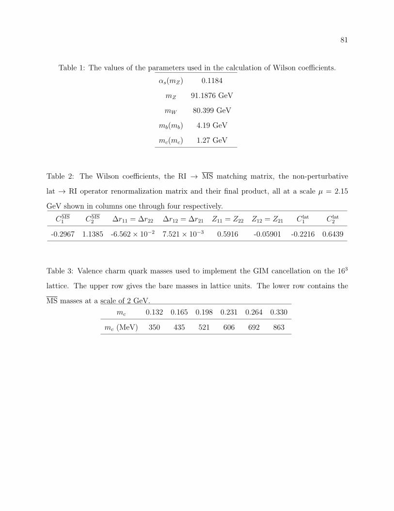
81
Table 1: The values of the parameters used in the calculation of Wilson coefficients.
αs(mZ) 0.1184
mZ 91.1876 GeV
mW 80.399 GeV
mb(mb) 4.19 GeV
mc(mc) 1.27 GeV
Table 2: The Wilson coefficients, the RI → MS matching matrix, the non-perturbative
lat → RI operator renormalization matrix and their final product, all at a scale µ = 2.15
GeV shown in columns one through four respectively.
CMS1 CMS
2 ∆r11 = ∆r22 ∆r12 = ∆r21 Z11 = Z22 Z12 = Z21 C lat1 C lat
2
-0.2967 1.1385 -6.562× 10⁻² 7.521× 10⁻³ 0.5916 -0.05901 -0.2216 0.6439
Table 3: Valence charm quark masses used to implement the GIM cancellation on the 163
lattice. The upper row gives the bare masses in lattice units. The lower row contains the
MS masses at a scale of 2 GeV.
mc 0.132 0.165 0.198 0.231 0.264 0.330
mc (MeV) 350 435 521 606 692 863
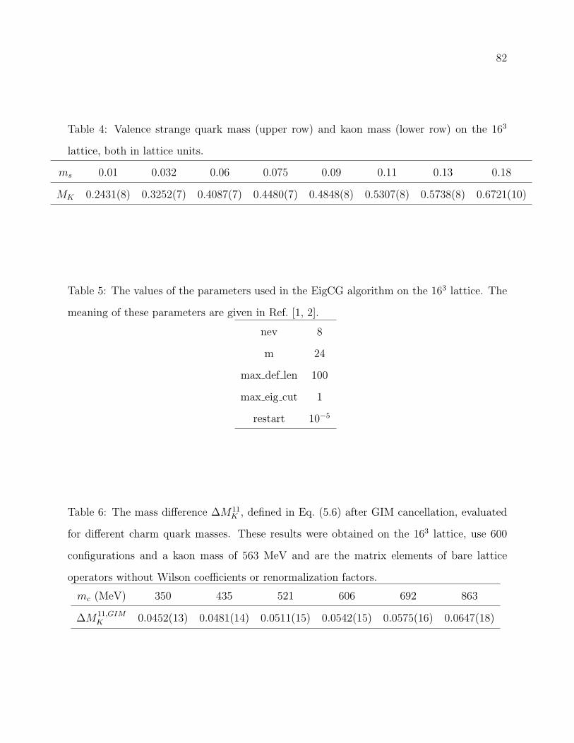
82
Table 4: Valence strange quark mass (upper row) and kaon mass (lower row) on the 163
lattice, both in lattice units.
ms 0.01 0.032 0.06 0.075 0.09 0.11 0.13 0.18
MK 0.2431(8) 0.3252(7) 0.4087(7) 0.4480(7) 0.4848(8) 0.5307(8) 0.5738(8) 0.6721(10)
Table 5: The values of the parameters used in the EigCG algorithm on the 163 lattice. The
meaning of these parameters are given in Ref. [1, 2].
nev 8
m 24
max def len 100
max eig cut 1
restart 10−5
Table 6: The mass difference ∆M11K , defined in Eq. (5.6) after GIM cancellation, evaluated
for different charm quark masses. These results were obtained on the 163 lattice, use 600
configurations and a kaon mass of 563 MeV and are the matrix elements of bare lattice
operators without Wilson coefficients or renormalization factors.
mc (MeV) 350 435 521 606 692 863
∆M11,GIMK 0.0452(13) 0.0481(14) 0.0511(15) 0.0542(15) 0.0575(16) 0.0647(18)
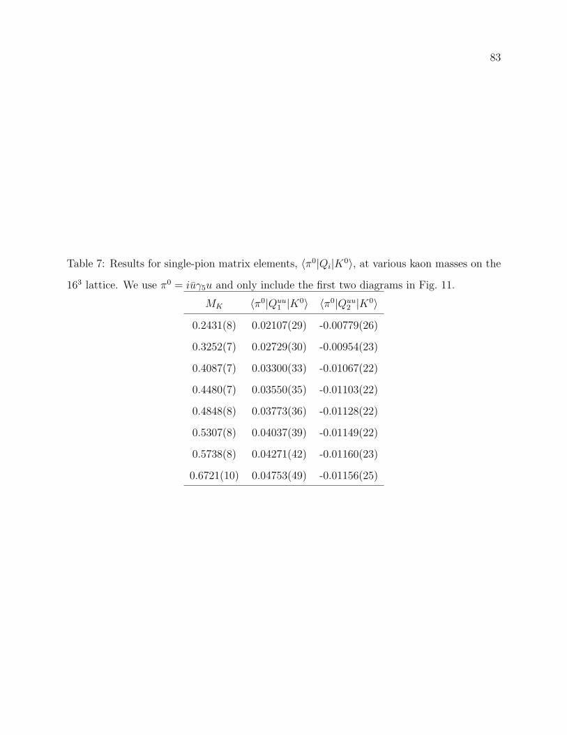
83
Table 7: Results for single-pion matrix elements, 〈π0|Qi|K0〉, at various kaon masses on the
163 lattice. We use π0 = iuγ5u and only include the first two diagrams in Fig. 11.
MK 〈π0|Quu1 |K0〉 〈π0|Quu
2 |K0〉
0.2431(8) 0.02107(29) -0.00779(26)
0.3252(7) 0.02729(30) -0.00954(23)
0.4087(7) 0.03300(33) -0.01067(22)
0.4480(7) 0.03550(35) -0.01103(22)
0.4848(8) 0.03773(36) -0.01128(22)
0.5307(8) 0.04037(39) -0.01149(22)
0.5738(8) 0.04271(42) -0.01160(23)
0.6721(10) 0.04753(49) -0.01156(25)

84
Table 8: Results for the integrated correlators for Mk = 563 MeV and mc = 863 MeV on
the 163 lattice. The quantities in columns two through four are the simple lattice integrated
correlators of the operator products Qqq′
i Qq′qj for each i, j = 1, 2, summed over the four values
of q, q′ = u, c, without Wilson coefficients or renormalization factors and have been scaled
to remove a factor 10−2.
T Q1 ·Q1 Q1 ·Q2 Q2 ·Q2
1 -1.422(26) 0.662(23) -0.1641(68)
2 -3.604(66) 1.450(51) -0.474(20)
3 -6.23(12) 2.401(87) -0.937(39)
4 -9.13(17) 3.48(13) -1.514(66)
5 -12.18(24) 4.67(18) -2.172(97)
6 -15.31(30) 5.93(23) -2.89(12)
7 -18.49(36) 7.22(29) -3.63(16)
8 -21.69(43) 8.54(35) -4.40(20)
9 -24.88(49) 9.84(41) -5.18(24)
10 -28.07(56) 11.14(49) -5.97(28)
11 -31.24(62) 12.39(58) -6.74(32)
12 -34.42(69) 13.62(68) -7.49(36)
13 -37.61(75) 14.88(79) -8.24(41)
14 -40.79(82) 16.11(91) -8.96(46)
15 -43.95(90) 17.3(10) -9.65(51)
16 -47.07(99) 18.5(12) -10.32(57)
17 -50.2(11) 19.6(14) -10.97(64)
18 -53.3(12) 20.7(16) -11.63(70)
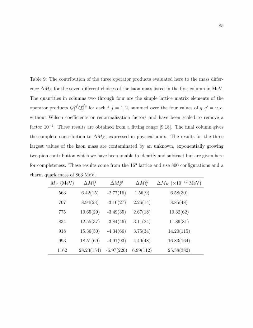
85
Table 9: The contribution of the three operator products evaluated here to the mass differ-
ence ∆MK for the seven different choices of the kaon mass listed in the first column in MeV.
The quantities in columns two through four are the simple lattice matrix elements of the
operator products Qqq′
i Qq′qj for each i, j = 1, 2, summed over the four values of q, q′ = u, c,
without Wilson coefficients or renormalization factors and have been scaled to remove a
factor 10−2. These results are obtained from a fitting range [9,18]. The final column gives
the complete contribution to ∆MK , expressed in physical units. The results for the three
largest values of the kaon mass are contaminated by an unknown, exponentially growing
two-pion contribution which we have been unable to identify and subtract but are given here
for completeness. These results come from the 163 lattice and use 800 configurations and a
charm quark mass of 863 MeV.
MK (MeV) ∆M11K ∆M12
K ∆M22K ∆MK (×10−12 MeV)
563 6.42(15) -2.77(16) 1.56(9) 6.58(30)
707 8.94(23) -3.16(27) 2.26(14) 8.85(48)
775 10.65(29) -3.49(35) 2.67(18) 10.32(62)
834 12.55(37) -3.84(46) 3.11(24) 11.89(81)
918 15.36(50) -4.34(66) 3.75(34) 14.20(115)
993 18.51(69) -4.91(93) 4.49(48) 16.83(164)
1162 28.23(154) -6.97(220) 6.99(112) 25.58(382)

86
Table 10: The quantity ∆MK for various charm quark masses and MK = 563 MeV on
the 163 lattice. Here the charm quark mass is given in the MS scheme at a scale µ = 2
GeV. The third and fourth columns give the lattice results and NLO perturbation result
respectively. For the perturbative result, the matching between four and three flavors is
done at µc = mc(mc). The second column contains the values of (mca)2 as an indication of
the size of finite lattice spacing errors which may corrupt the comparison between the lattice
and NLO perturbative results.
mc (MeV) (mca)2 ∆MK (10−15 GeV) ∆MNLO
K (10−15 GeV)
350 0.04 4.76(27) 3.24
435 0.06 5.06(29) 2.82
521 0.09 5.36(31) 2.63
606 0.12 5.66(32) 2.56
692 0.16 5.96(33) 2.56
863 0.25 6.58(35) 2.68
1086 0.39 7.37(38) 2.99
1449 0.70 8.61(41) 3.67

87
Table 11: The values of the parameters used in the Lanczos algorithm on the 243 lattice.
The meaning of these parameters are given in Ref. [3].
Mass 0.005
Stop rsd 10−9
QR rsd 10−14
Operator D†D
Precondition 1
K 305
M 340
Neig 300
npoly 100
α 5.5
β 0.12
µ 0

88
Table 12: Results for the integrated correlators on the 243 lattice. The kaon sources are
separated by 31 lattice units. The quantities in columns two through four are the simple
lattice integrated correlators of the operator products Qqq′
i Qq′qj for each i, j = 1, 2, summed
over the four values of q, q′ = u, c, without Wilson coefficients or renormalization factors and
have been scaled to remove a factor 10−4.
T Q1 ·Q1 Q1 ·Q2 Q2 ·Q2
1 0.14(20) -0.220(93) -0.188(5)
2 -0.44(40) -0.50(19) -0.496(14)
3 -1.37(60) -0.77(28) -0.921(27)
4 -2.51(80) -0.99(38) -1.438(46)
5 -3.73(99) -1.18(49) -2.017(71)
6 -5.0(12) -1.34(60) -2.64(10)
7 -6.3(14) -1.48(72) -3.28(15)
8 -7.6(16) -1.66(86) -3.92(21)
9 -8.8(18) -1.9(10) -4.57(29)
10 -10.1(20) -2.1(12) -5.21(40)
11 -11.3(23) -2.4(15) -5.85(54)
12 -12.5(25) -2.8(18) -6.46(73)
13 -13.5(28) -3.5(22) -6.99(99)
14 -14.4(31) -4.4(28) -7.43(135)
15 -14.9(35) -5.7(35) -7.7(18)
16 -15.4(40) -6.7(46) -8.2(25)
17 -15.1(47) -8.0(61) -8.7(35)
18 -14.5(56) -8.4(81) -9.5(47)
19 -14.1(69) -7.4(107) -10.7(65)
20 -13.8(87) -5.1(143) -13.3(90)
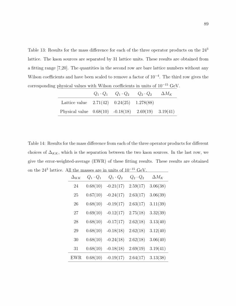
89
Table 13: Results for the mass difference for each of the three operator products on the 243
lattice. The kaon sources are separated by 31 lattice units. These results are obtained from
a fitting range [7,20]. The quantities in the second row are bare lattice numbers without any
Wilson coefficients and have been scaled to remove a factor of 10−4. The third row gives the
corresponding physical values with Wilson coefficients in units of 10−15 GeV.
Q1 ·Q1 Q1 ·Q2 Q2 ·Q2 ∆MK
Lattice value 2.71(42) 0.24(25) 1.278(88)
Physical value 0.68(10) -0.18(18) 2.69(19) 3.19(41)
Table 14: Results for the mass difference from each of the three operator products for different
choices of ∆KK , which is the separation between the two kaon sources. In the last row, we
give the error-weighted-average (EWR) of these fitting results. These results are obtained
on the 243 lattice. All the masses are in units of 10−15 GeV.
∆KK Q1 ·Q1 Q1 ·Q2 Q2 ·Q2 ∆MK
24 0.68(10) -0.21(17) 2.59(17) 3.06(38)
25 0.67(10) -0.24(17) 2.63(17) 3.06(39)
26 0.68(10) -0.19(17) 2.63(17) 3.11(39)
27 0.69(10) -0.12(17) 2.75(18) 3.32(39)
28 0.68(10) -0.17(17) 2.62(18) 3.13(40)
29 0.68(10) -0.18(18) 2.62(18) 3.12(40)
30 0.68(10) -0.24(18) 2.62(18) 3.06(40)
31 0.68(10) -0.18(18) 2.69(19) 3.19(41)
EWR 0.68(10) -0.19(17) 2.64(17) 3.13(38)

90
Table 15: Results for the mass difference from each of the three operator products for different
choices of Tmin, which is the minimum fitting time. We fix ∆min = 6, which is the minimum
separation between the kaon sources and the weak Hamiltonians. These results are obtained
on the 243 lattice. All the masses are in units of 10−15 GeV.
∆min Tmin Q1 ·Q1 Q1 ·Q2 Q2 ·Q2 ∆MK
6
7 0.68(10) -0.18(18) 2.69(19) 3.19(41)
8 0.68(10) -0.11(20) 2.85(24) 3.42(48)
9 0.68(11) -0.18(25) 2.69(34) 3.18(63)
Table 16: Fitting results for the mass difference from each of the three operator products
for different choices of ∆min, which is the minimum separation between the kaon sources and
the weak Hamiltonians. The minimal fitting time Tmin is 7. These results are obtained on
the 243 lattice. All the masses are in units of 10−15 GeV.
Tmin ∆min Q1 ·Q1 Q1 ·Q2 Q2 ·Q2 ∆MK
7
6 0.68(10) -0.18(18) 2.69(19) 3.19(41)
7 0.68(10) -0.20(18) 2.64(19) 3.13(41)
8 0.67(10) -0.19(18) 2.61(19) 3.09(41)
Table 17: Comparison of mass difference from different types of diagrams on the 243 lattice.
We choose ∆min = 8, which is the minimum separation between the kaon sources and the
weak Hamiltonians. These results are obtained on the 243 lattice. All the numbers here are
in units of 10−15 GeV.
Diagrams Fitting range Q1 ·Q1 Q1 ·Q2 Q2 ·Q2 ∆MK
Type 1 [9,16] 1.330(7) 0.075(32) -0.978(58) 0.427(91)
Type 2 [12,16] 0.164(3) 1.600(24) 4.807(50) 6.572(75)
Type 3 [7,16] 0.009(3) 0.187(17) 0.619(32) 0.816(47)
Type 4 [7,16] -0.541(21) -1.77(10) -1.33(18) -3.64(29)

91
Table 18: Comparison of mass difference for different values of cs. The value of cp is chosen
to be 1. cs and cp are defined in Eq. 6.1. The value of cs = −1.14(26) will eliminate the
η intermediate state. We choose ∆min = 6, which is the minimum separation between the
kaon sources and the weak Hamiltonians. The minimal fitting time Tmin is 7. These results
are obtained on the 243 lattice. All the numbers here are in units of 10−15 GeV.
cs Q1 ·Q1 Q1 ·Q2 Q2 ·Q2 ∆MK
-1 0.68(12) -0.20(21) 2.63(27) 3.12(40)
0 0.68(10) -0.18(18) 2.69(19) 3.19(41)
1 0.672(88) -0.15(28) 2.69(25) 3.21(59)
-1.14(26) 0.661(58) -0.14(19) 2.70(19) 3.22(40)
Table 19: The mass difference for cs = 1 and cp = 0. cs and cp are defined in Eq. 6.1. ∆min
is the minimum separation between the kaon sources and the weak Hamiltonians. These
results are obtained on the 243 lattice. All the numbers here are in units of 10−15 GeV.
∆min Fitting range ∆M11 ∆M12 ∆M22 ∆MK
6 [7,12] 0.56(10) -1.35(19) -0.79(23) -1.57(44)
10 [7,12] 0.55(11) -1.43(22) -0.78(32) -1.66(55)
Table 20: Contribution to the mass differences from the π0 and the vacuum states. We do
not add sd or sγ5d operators to the weak Hamiltonian while evaluating these values. These
results are obtained on the 243 lattice. All the numbers are in units of 10−15 GeV.
State ∆M11 ∆M12 ∆M22 ∆MK
π0 0.00609(15) -0.1258(13) 0.6498(41) 0.5301(47)
η 0.330(99) 0.07(14) 0.04(14) 0.40(23)
vacuum -0.863(40) -9.630(31) -26.866(78) -37.36(11)
92
Figures
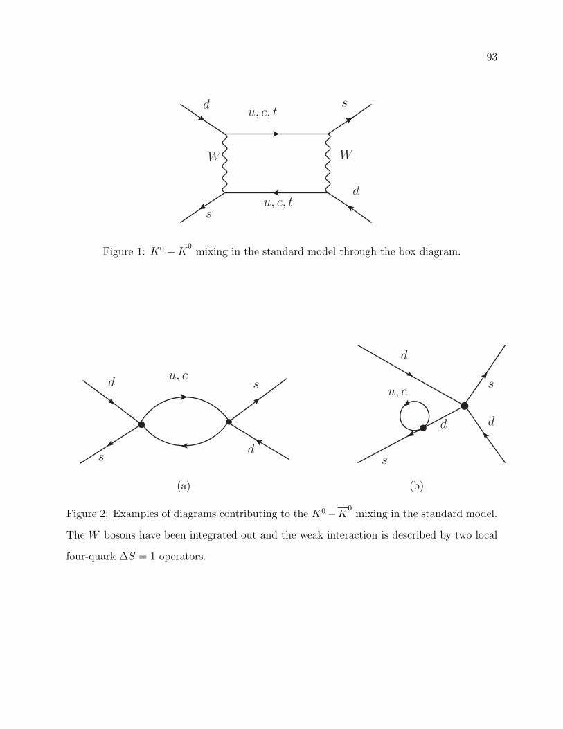
93
d
d
s
s
u, c, t
u, c, t
W W
Figure 1: K0 −K0mixing in the standard model through the box diagram.
d
d
s
s
u, c
d
d
s
s
d
u, c
(a) (b)
Figure 2: Examples of diagrams contributing to the K0−K0mixing in the standard model.
The W bosons have been integrated out and the weak interaction is described by two local
four-quark ∆S = 1 operators.
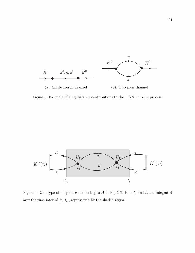
94
K0K
0π0, η, η′
K0K
0
π
π
(a). Single meson channel (b). Two pion channel
Figure 3: Example of long distance contributions to the K0-K0mixing process.
d
d
s
s
u
u
HW HW
t1 t2K0†(ti) K
0(tf)
ta tb
Figure 4: One type of diagram contributing to A in Eq. 3.6. Here t2 and t1 are integrated
over the time interval [ta, tb], represented by the shaded region.
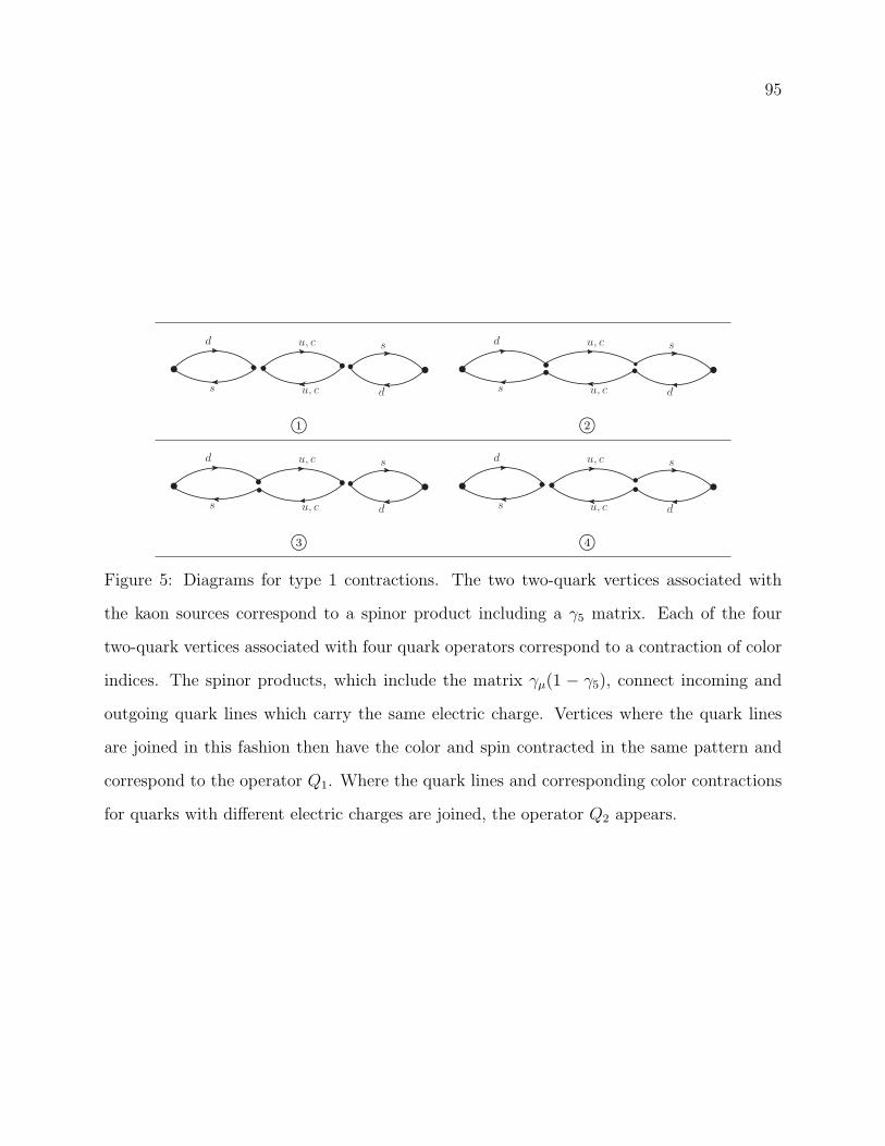
95
u, c
u, c
d
s d
s u, c
u, c
d
s d
s
1© 2©
u, c
u, c
d
s d
s u, c
u, c
d
s d
s
3© 4©
Figure 5: Diagrams for type 1 contractions. The two two-quark vertices associated with
the kaon sources correspond to a spinor product including a γ5 matrix. Each of the four
two-quark vertices associated with four quark operators correspond to a contraction of color
indices. The spinor products, which include the matrix γµ(1 − γ5), connect incoming and
outgoing quark lines which carry the same electric charge. Vertices where the quark lines
are joined in this fashion then have the color and spin contracted in the same pattern and
correspond to the operator Q1. Where the quark lines and corresponding color contractions
for quarks with different electric charges are joined, the operator Q2 appears.
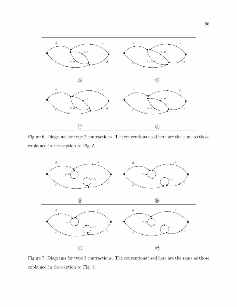
96
d
s d
s
c, u
c, u
d
s d
s
c, u
c, u
5© 6©
d
s d
s
c, u
c, u
d
s d
s
c, u
c, u
7© 8©
Figure 6: Diagrams for type 2 contractions. The conventions used here are the same as those
explained in the caption to Fig. 5.
d s
sd
c, u
c, u
d s
sd
c, u
c, u
9© 10©
d s
sd
c, u
c, u
d s
sd
c, u
c, u
11© 12©
Figure 7: Diagrams for type 3 contractions. The conventions used here are the same as those
explained in the caption to Fig. 5.

97
d
s d
su, c u, c d
s d
su, c u, c
13© 14©
d
s d
su, c u, c d
s d
su, c u, c
15© 16©
Figure 8: Diagrams for type 3 contractions. The conventions used here are the same as those
explained in the caption to Fig. 5.
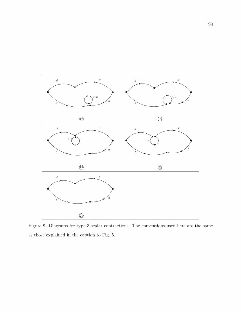
98
d s
sd
c, u
d s
sd
c, u
17© 18©
d s
sd
c, u
d s
sd
c, u
19© 20©
d s
sd
21©
Figure 9: Diagrams for type 3-scalar contractions. The conventions used here are the same
as those explained in the caption to Fig. 5.
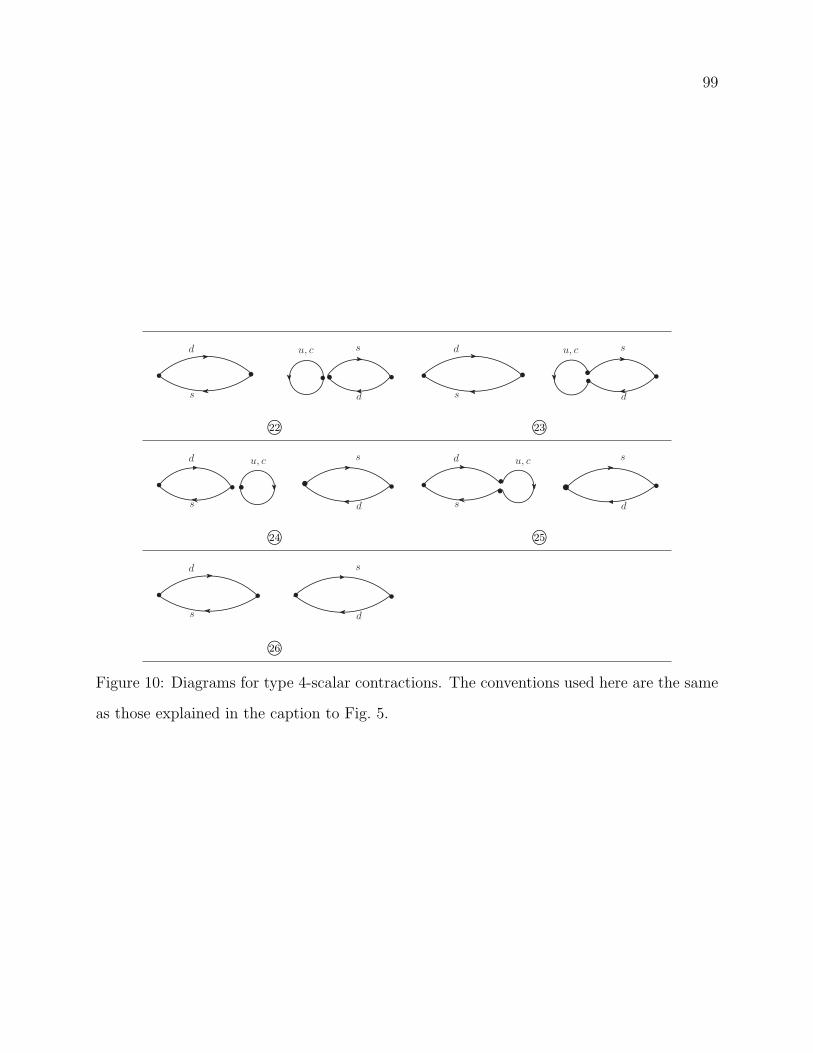
99
d
s d
su, c d
s d
su, c
22© 23©
d
s d
su, c d
s d
su, c
24© 25©
d
s d
s
26©
Figure 10: Diagrams for type 4-scalar contractions. The conventions used here are the same
as those explained in the caption to Fig. 5.
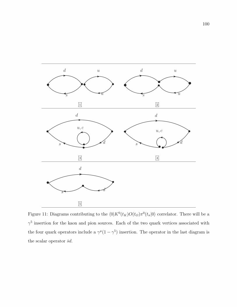
100
d
s
u
u
d
s
u
u
1 2
d
ds
u, c
d
ds
u, c
3 4
d
ds
5
Figure 11: Diagrams contributing to the 〈0|K0(tK)O(tO)π0(tπ|0〉 correlator. There will be a
γ5 insertion for the kaon and pion sources. Each of the two quark vertices associated with
the four quark operators include a γµ(1− γ5) insertion. The operator in the last diagram is
the scalar operator sd.
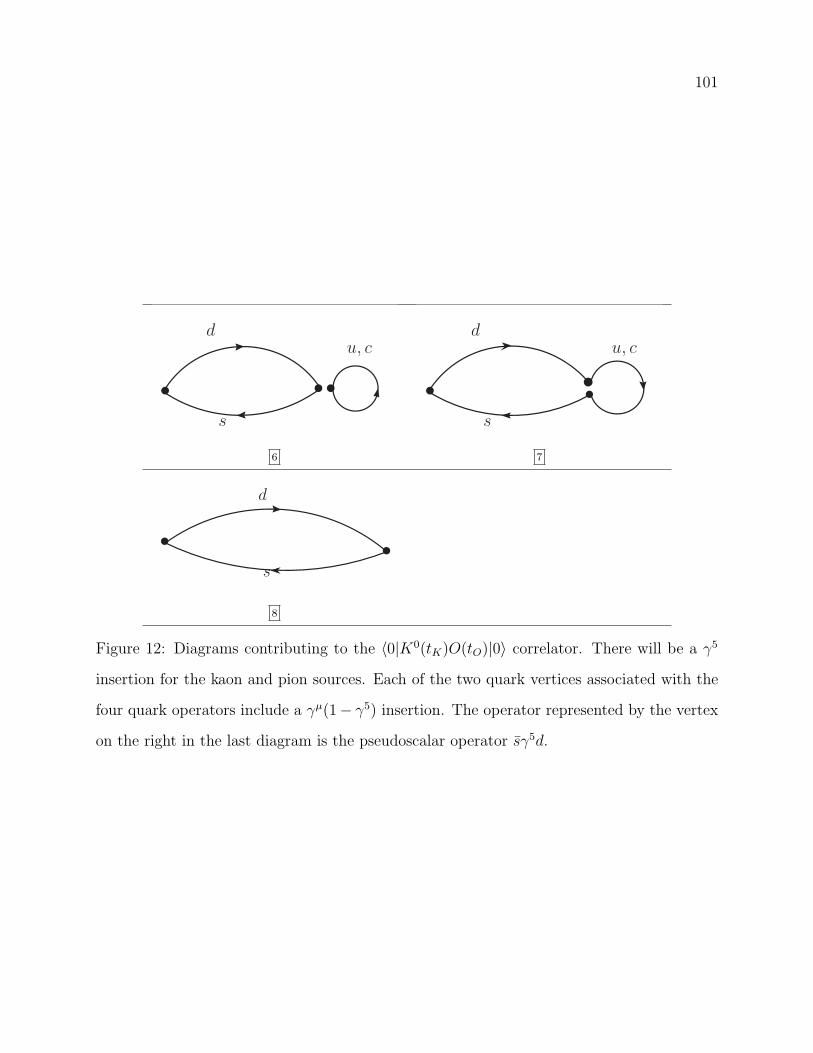
101
d
s
u, cd
s
u, c
6 7
d
s
8
Figure 12: Diagrams contributing to the 〈0|K0(tK)O(tO)|0〉 correlator. There will be a γ5
insertion for the kaon and pion sources. Each of the two quark vertices associated with the
four quark operators include a γµ(1− γ5) insertion. The operator represented by the vertex
on the right in the last diagram is the pseudoscalar operator sγ5d.
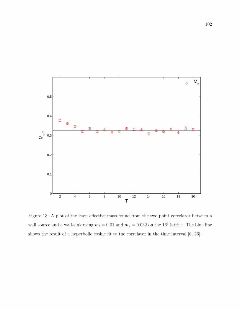
102
2 4 6 8 10 12 14 16 18 200
0.1
0.2
0.3
0.4
0.5
T
Mef
f
M
K
Figure 13: A plot of the kaon effective mass found from the two point correlator between a
wall source and a wall-sink using ml = 0.01 and ms = 0.032 on the 163 lattice. The blue line
shows the result of a hyperbolic cosine fit to the correlator in the time interval [6, 26].
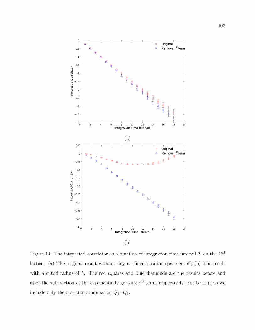
103
0 2 4 6 8 10 12 14 16 18 20−5
−4.5
−4
−3.5
−3
−2.5
−2
−1.5
−1
−0.5
0
Integration Time Interval
Inte
grat
ed C
orre
lato
r
OriginalRemove π0 term
(a)
0 2 4 6 8 10 12 14 16 18 20−0.45
−0.4
−0.35
−0.3
−0.25
−0.2
−0.15
−0.1
−0.05
0
0.05
Integration Time Interval
Inte
grat
ed C
orre
lato
r
OriginalRemove π0 term
(b)
Figure 14: The integrated correlator as a function of integration time interval T on the 163
lattice. (a) The original result without any artificial position-space cutoff; (b) The result
with a cutoff radius of 5. The red squares and blue diamonds are the results before and
after the subtraction of the exponentially growing π0 term, respectively. For both plots we
include only the operator combination Q1 ·Q1.

104
1 1.5 2 2.5 3 3.5 4 4.5 5 5.5 60
0.1
0.2
0.3
0.4
0.5
0.6
0.7
0.8
0.9
1
Cutoff Radius
Mas
s di
ffere
nce
Mass DiffereceQuadratic Fit
Figure 15: The mass difference ∆M11K defined in Eq. (5.6) for different values of the cutoff
radius R on the 163 lattice. The blue curve is the two parameter fit to a 1/R2 behavior as
defined in Eq. (5.7)
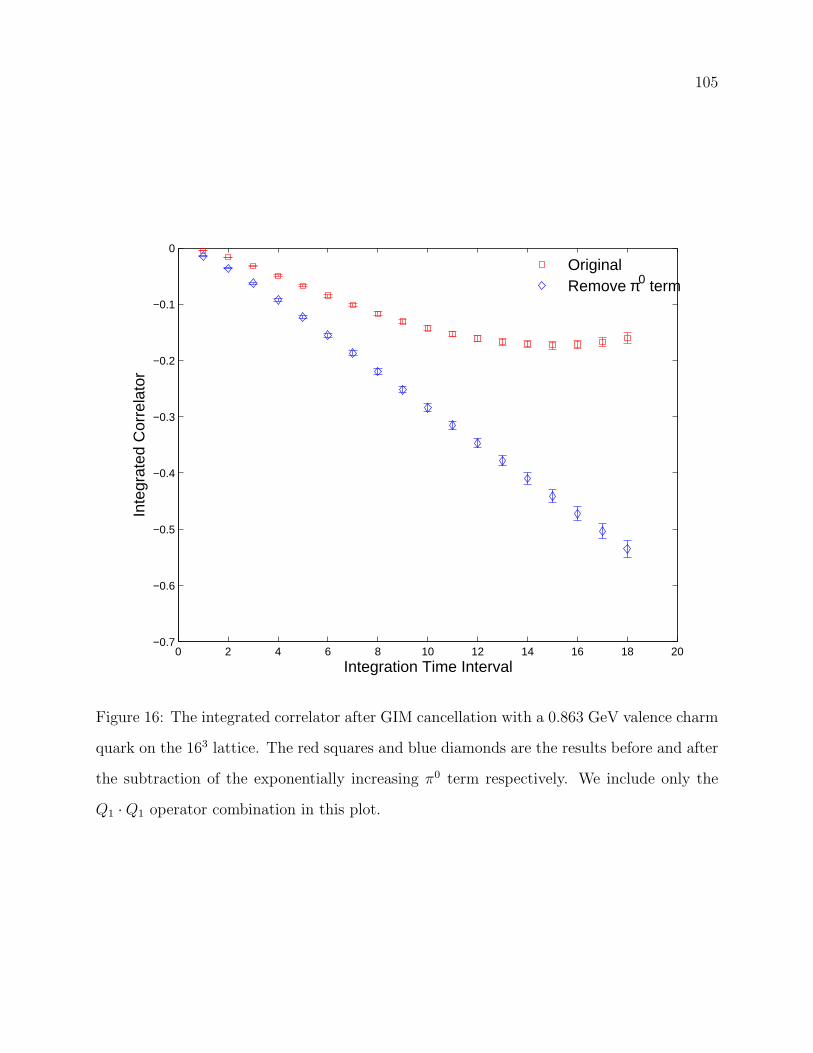
105
0 2 4 6 8 10 12 14 16 18 20−0.7
−0.6
−0.5
−0.4
−0.3
−0.2
−0.1
0
Integration Time Interval
Inte
grat
ed C
orre
lato
r
OriginalRemove π0 term
Figure 16: The integrated correlator after GIM cancellation with a 0.863 GeV valence charm
quark on the 163 lattice. The red squares and blue diamonds are the results before and after
the subtraction of the exponentially increasing π0 term respectively. We include only the
Q1 ·Q1 operator combination in this plot.

106
0.3 0.4 0.5 0.6 0.7 0.8 0.90
0.01
0.02
0.03
0.04
0.05
0.06
0.07
Valence Charm Quark Mass / Gev
Mas
s di
ffere
nce
Figure 17: The mass difference ∆M11K , defined in Eq. (5.6) after GIM cancellation as a
function of the valence charm quark mass. These results are obtained on the 163 lattice.
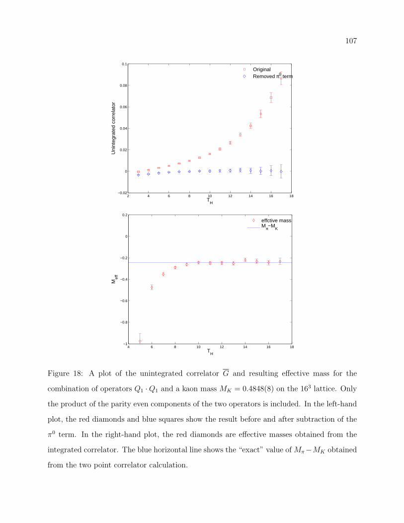
107
2 4 6 8 10 12 14 16 18−0.02
0
0.02
0.04
0.06
0.08
0.1
TH
Uni
nteg
rate
d co
rrel
ator
OriginalRemoved π0 term
4 6 8 10 12 14 16 18−1
−0.8
−0.6
−0.4
−0.2
0
0.2
TH
Mef
f
effctive massMπ−M
K
Figure 18: A plot of the unintegrated correlator G and resulting effective mass for the
combination of operators Q1 ·Q1 and a kaon mass MK = 0.4848(8) on the 163 lattice. Only
the product of the parity even components of the two operators is included. In the left-hand
plot, the red diamonds and blue squares show the result before and after subtraction of the
π0 term. In the right-hand plot, the red diamonds are effective masses obtained from the
integrated correlator. The blue horizontal line shows the “exact” value of Mπ−MK obtained
from the two point correlator calculation.
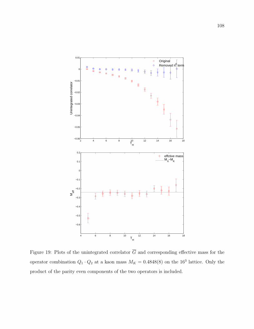
108
2 4 6 8 10 12 14 16 18−0.06
−0.05
−0.04
−0.03
−0.02
−0.01
0
0.01
TH
Uni
nteg
rate
d co
rrel
ator
OriginalRemoved π0 term
4 6 8 10 12 14 16 18
−0.6
−0.5
−0.4
−0.3
−0.2
−0.1
0
0.1
0.2
TH
Mef
f
effctive massMπ−M
K
Figure 19: Plots of the unintegrated correlator G and corresponding effective mass for the
operator combination Q1 · Q2 at a kaon mass MK = 0.4848(8) on the 163 lattice. Only the
product of the parity even components of the two operators is included.
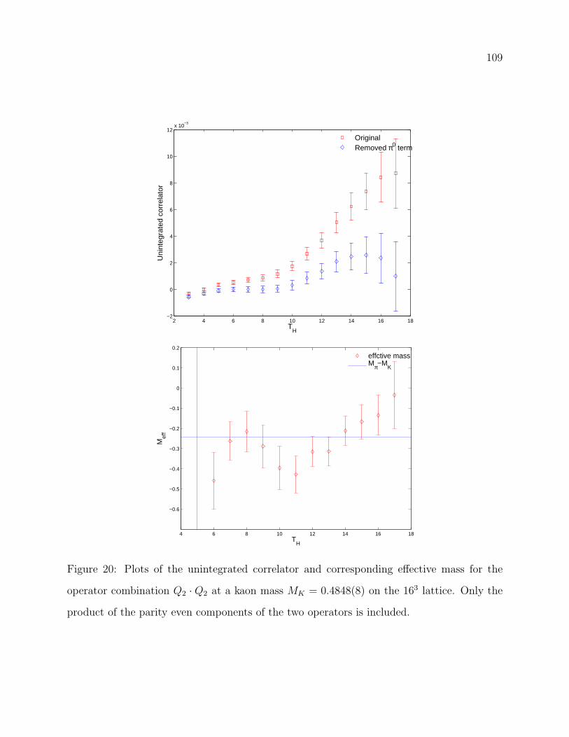
109
2 4 6 8 10 12 14 16 18−2
0
2
4
6
8
10
12x 10
−3
TH
Uni
nteg
rate
d co
rrel
ator
OriginalRemoved π0 term
4 6 8 10 12 14 16 18
−0.6
−0.5
−0.4
−0.3
−0.2
−0.1
0
0.1
0.2
TH
Mef
f
effctive massMπ−M
K
Figure 20: Plots of the unintegrated correlator and corresponding effective mass for the
operator combination Q2 · Q2 at a kaon mass MK = 0.4848(8) on the 163 lattice. Only the
product of the parity even components of the two operators is included.
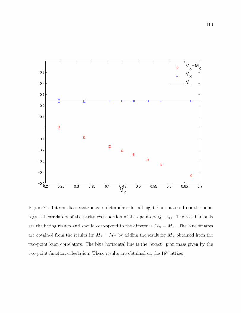
110
0.2 0.25 0.3 0.35 0.4 0.45 0.5 0.55 0.6 0.65 0.7−0.5
−0.4
−0.3
−0.2
−0.1
0
0.1
0.2
0.3
0.4
0.5
MK
M
X−M
K
MX
Mπ
Figure 21: Intermediate state masses determined for all eight kaon masses from the unin-
tegrated correlators of the parity even portion of the operators Q1 · Q1. The red diamonds
are the fitting results and should correspond to the difference MX −MK . The blue squares
are obtained from the results for MX −MK by adding the result for MK obtained from the
two-point kaon correlators. The blue horizontal line is the “exact” pion mass given by the
two point function calculation. These results are obtained on the 163 lattice.
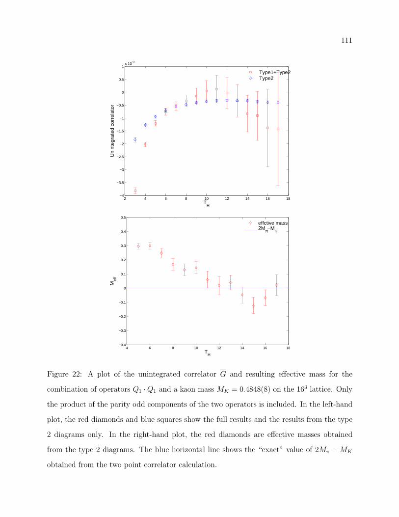
111
2 4 6 8 10 12 14 16 18−4
−3.5
−3
−2.5
−2
−1.5
−1
−0.5
0
0.5
1x 10
−3
TH
Uni
nteg
rate
d co
rrel
ator
Type1+Type2Type2
4 6 8 10 12 14 16 18−0.4
−0.3
−0.2
−0.1
0
0.1
0.2
0.3
0.4
0.5
TH
Mef
f
effctive mass2Mπ−M
K
Figure 22: A plot of the unintegrated correlator G and resulting effective mass for the
combination of operators Q1 ·Q1 and a kaon mass MK = 0.4848(8) on the 163 lattice. Only
the product of the parity odd components of the two operators is included. In the left-hand
plot, the red diamonds and blue squares show the full results and the results from the type
2 diagrams only. In the right-hand plot, the red diamonds are effective masses obtained
from the type 2 diagrams. The blue horizontal line shows the “exact” value of 2Mπ −MK
obtained from the two point correlator calculation.
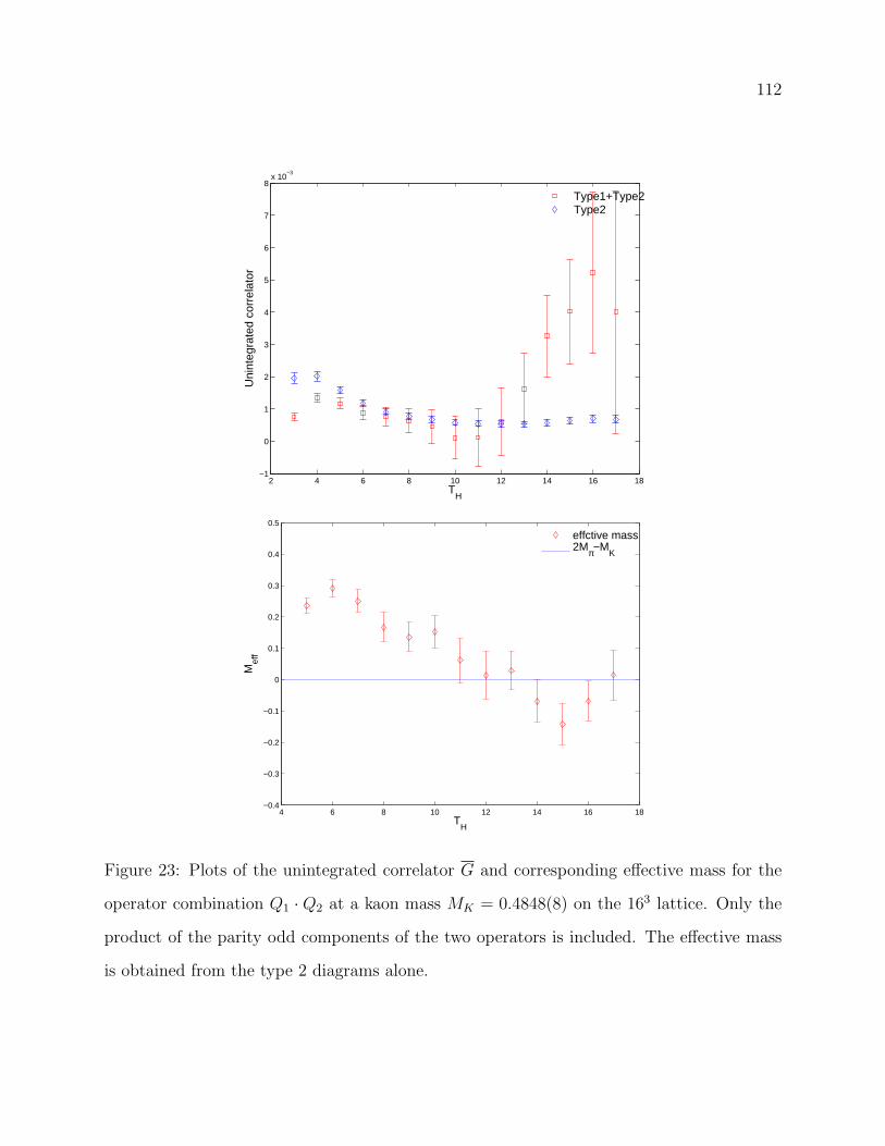
112
2 4 6 8 10 12 14 16 18−1
0
1
2
3
4
5
6
7
8x 10
−3
TH
Uni
nteg
rate
d co
rrel
ator
Type1+Type2Type2
4 6 8 10 12 14 16 18−0.4
−0.3
−0.2
−0.1
0
0.1
0.2
0.3
0.4
0.5
TH
Mef
f
effctive mass2Mπ−M
K
Figure 23: Plots of the unintegrated correlator G and corresponding effective mass for the
operator combination Q1 · Q2 at a kaon mass MK = 0.4848(8) on the 163 lattice. Only the
product of the parity odd components of the two operators is included. The effective mass
is obtained from the type 2 diagrams alone.
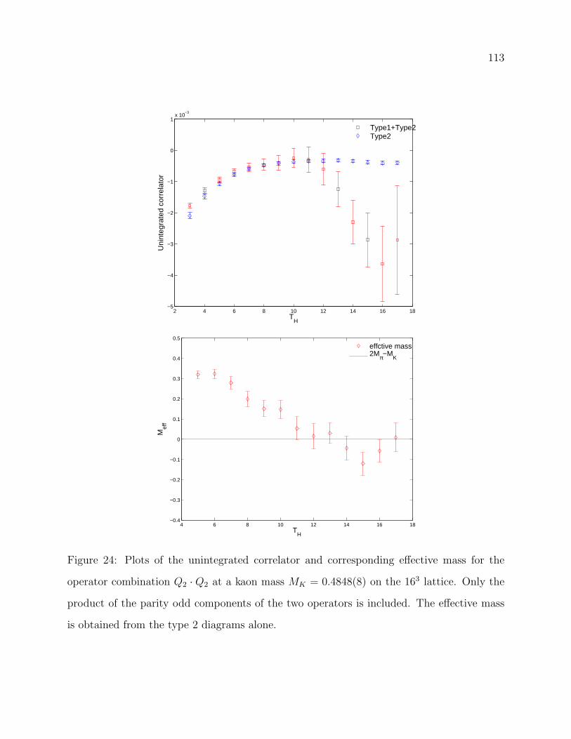
113
2 4 6 8 10 12 14 16 18−5
−4
−3
−2
−1
0
1x 10
−3
TH
Uni
nteg
rate
d co
rrel
ator
Type1+Type2Type2
4 6 8 10 12 14 16 18−0.4
−0.3
−0.2
−0.1
0
0.1
0.2
0.3
0.4
0.5
TH
Mef
f
effctive mass2Mπ−M
K
Figure 24: Plots of the unintegrated correlator and corresponding effective mass for the
operator combination Q2 · Q2 at a kaon mass MK = 0.4848(8) on the 163 lattice. Only the
product of the parity odd components of the two operators is included. The effective mass
is obtained from the type 2 diagrams alone.
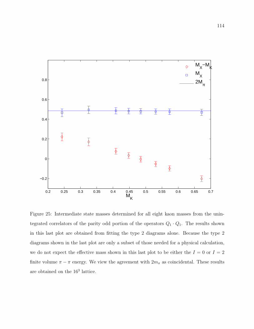
114
0.2 0.25 0.3 0.35 0.4 0.45 0.5 0.55 0.6 0.65 0.7
−0.2
0
0.2
0.4
0.6
0.8
MK
M
X−M
K
MX
2Mπ
Figure 25: Intermediate state masses determined for all eight kaon masses from the unin-
tegrated correlators of the parity odd portion of the operators Q1 · Q1. The results shown
in this last plot are obtained from fitting the type 2 diagrams alone. Because the type 2
diagrams shown in the last plot are only a subset of those needed for a physical calculation,
we do not expect the effective mass shown in this last plot to be either the I = 0 or I = 2
finite volume π− π energy. We view the agreement with 2mπ as coincidental. These results
are obtained on the 163 lattice.
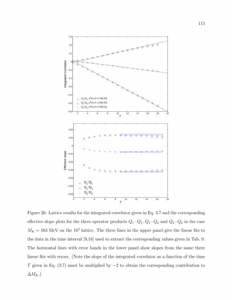
115
2 4 6 8 10 12 14 16 18 20−0.6
−0.5
−0.4
−0.3
−0.2
−0.1
0
0.1
0.2
0.3
T
Inte
grat
ed C
orre
lato
r
Q1⋅ Q
1, χ2/d.o.f= 0.74(0.65)
Q1⋅ Q
2, χ2/d.o.f= 1.03(0.63)
Q2⋅ Q
2, χ2/d.o.f= 0.70(0.51)
0 2 4 6 8 10 12 14 16 18
−0.06
−0.05
−0.04
−0.03
−0.02
−0.01
0
0.01
0.02
T
Effe
ctiv
e sl
ope
Q1⋅ Q
1
Q1⋅ Q
2
Q2⋅ Q
2
Figure 26: Lattice results for the integrated correlator given in Eq. 3.7 and the corresponding
effective slope plots for the three operator products Q1 ·Q1, Q1 ·Q2 and Q2 ·Q2 in the case
MK = 563 MeV on the 163 lattice. The three lines in the upper panel give the linear fits to
the data in the time interval [9,18] used to extract the corresponding values given in Tab. 9.
The horizontal lines with error bands in the lower panel show slopes from the same three
linear fits with errors. (Note the slope of the integrated correlator as a function of the time
T given in Eq. (3.7) must be multiplied by −2 to obtain the corresponding contribution to
∆MK .)
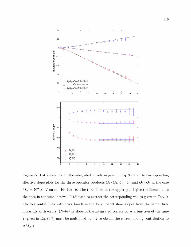
116
2 4 6 8 10 12 14 16 18 20−1
−0.8
−0.6
−0.4
−0.2
0
0.2
0.4
T
Inte
grat
ed C
orre
lato
r
Q1⋅ Q
1, χ2/d.o.f= 0.53(0.52)
Q1⋅ Q
2, χ2/d.o.f= 0.65(0.50)
Q2⋅ Q
2, χ2/d.o.f= 0.36(0.37)
0 2 4 6 8 10 12 14 16 18
−0.08
−0.06
−0.04
−0.02
0
0.02
T
Effe
ctiv
e sl
ope
Q1⋅ Q
1
Q1⋅ Q
2
Q2⋅ Q
2
Figure 27: Lattice results for the integrated correlator given in Eq. 3.7 and the corresponding
effective slope plots for the three operator products Q1 ·Q1, Q1 ·Q2 and Q2 ·Q2 in the case
MK = 707 MeV on the 163 lattice. The three lines in the upper panel give the linear fits to
the data in the time interval [9,18] used to extract the corresponding values given in Tab. 9.
The horizontal lines with error bands in the lower panel show slopes from the same three
linear fits with errors. (Note the slope of the integrated correlator as a function of the time
T given in Eq. (3.7) must be multiplied by −2 to obtain the corresponding contribution to
∆MK .)
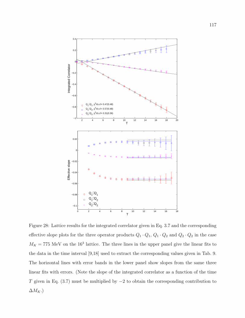
117
2 4 6 8 10 12 14 16 18 20−1
−0.8
−0.6
−0.4
−0.2
0
0.2
0.4
T
Inte
grat
ed C
orre
lato
r
Q1⋅ Q
1, χ2/d.o.f= 0.47(0.48)
Q1⋅ Q
2, χ2/d.o.f= 0.57(0.48)
Q2⋅ Q
2, χ2/d.o.f= 0.31(0.36)
0 2 4 6 8 10 12 14 16 18
−0.1
−0.08
−0.06
−0.04
−0.02
0
0.02
T
Effe
ctiv
e sl
ope
Q1⋅ Q
1
Q1⋅ Q
2
Q2⋅ Q
2
Figure 28: Lattice results for the integrated correlator given in Eq. 3.7 and the corresponding
effective slope plots for the three operator products Q1 ·Q1, Q1 ·Q2 and Q2 ·Q2 in the case
MK = 775 MeV on the 163 lattice. The three lines in the upper panel give the linear fits to
the data in the time interval [9,18] used to extract the corresponding values given in Tab. 9.
The horizontal lines with error bands in the lower panel show slopes from the same three
linear fits with errors. (Note the slope of the integrated correlator as a function of the time
T given in Eq. (3.7) must be multiplied by −2 to obtain the corresponding contribution to
∆MK .)
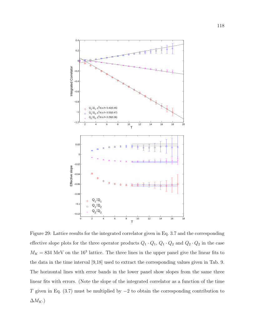
118
2 4 6 8 10 12 14 16 18 20−1.2
−1
−0.8
−0.6
−0.4
−0.2
0
0.2
0.4
T
Inte
grat
ed C
orre
lato
r
Q1⋅ Q
1, χ2/d.o.f= 0.42(0.45)
Q1⋅ Q
2, χ2/d.o.f= 0.53(0.47)
Q2⋅ Q
2, χ2/d.o.f= 0.29(0.36)
0 2 4 6 8 10 12 14 16 18
−0.12
−0.1
−0.08
−0.06
−0.04
−0.02
0
0.02
T
Effe
ctiv
e sl
ope
Q1⋅ Q
1
Q1⋅ Q
2
Q2⋅ Q
2
Figure 29: Lattice results for the integrated correlator given in Eq. 3.7 and the corresponding
effective slope plots for the three operator products Q1 ·Q1, Q1 ·Q2 and Q2 ·Q2 in the case
MK = 834 MeV on the 163 lattice. The three lines in the upper panel give the linear fits to
the data in the time interval [9,18] used to extract the corresponding values given in Tab. 9.
The horizontal lines with error bands in the lower panel show slopes from the same three
linear fits with errors. (Note the slope of the integrated correlator as a function of the time
T given in Eq. (3.7) must be multiplied by −2 to obtain the corresponding contribution to
∆MK .)
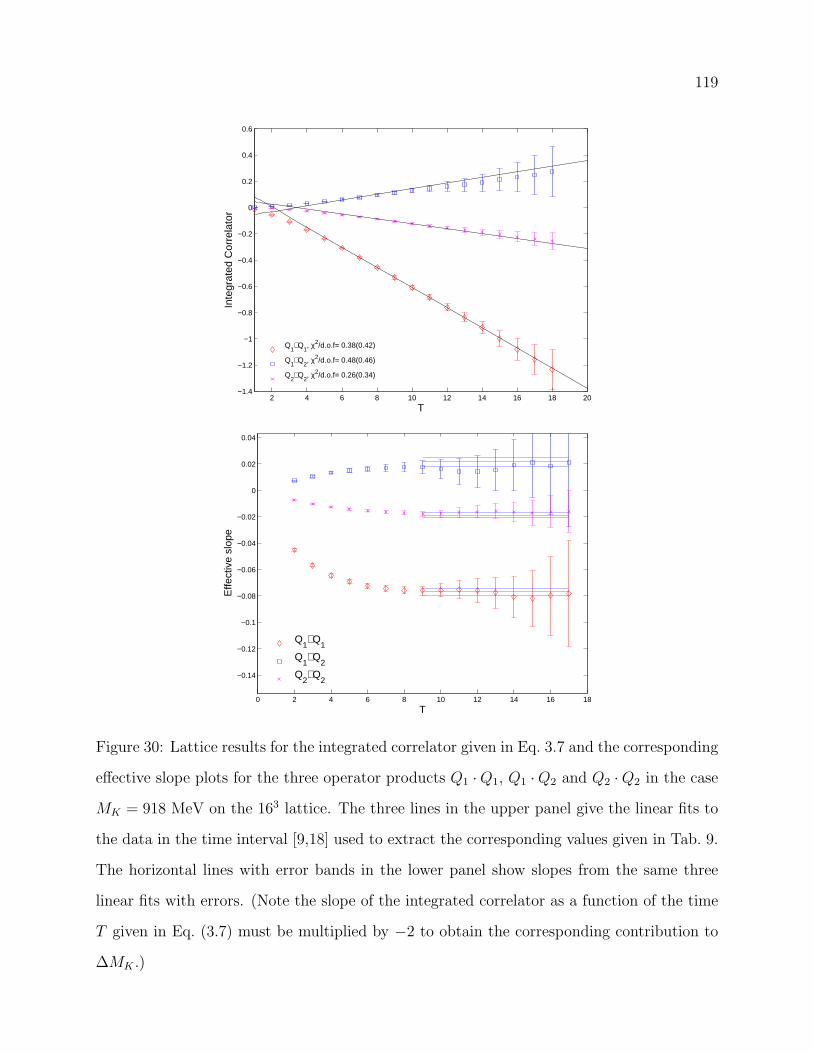
119
2 4 6 8 10 12 14 16 18 20−1.4
−1.2
−1
−0.8
−0.6
−0.4
−0.2
0
0.2
0.4
0.6
T
Inte
grat
ed C
orre
lato
r
Q1⋅ Q
1, χ2/d.o.f= 0.38(0.42)
Q1⋅ Q
2, χ2/d.o.f= 0.48(0.46)
Q2⋅ Q
2, χ2/d.o.f= 0.26(0.34)
0 2 4 6 8 10 12 14 16 18
−0.14
−0.12
−0.1
−0.08
−0.06
−0.04
−0.02
0
0.02
0.04
T
Effe
ctiv
e sl
ope
Q1⋅ Q
1
Q1⋅ Q
2
Q2⋅ Q
2
Figure 30: Lattice results for the integrated correlator given in Eq. 3.7 and the corresponding
effective slope plots for the three operator products Q1 ·Q1, Q1 ·Q2 and Q2 ·Q2 in the case
MK = 918 MeV on the 163 lattice. The three lines in the upper panel give the linear fits to
the data in the time interval [9,18] used to extract the corresponding values given in Tab. 9.
The horizontal lines with error bands in the lower panel show slopes from the same three
linear fits with errors. (Note the slope of the integrated correlator as a function of the time
T given in Eq. (3.7) must be multiplied by −2 to obtain the corresponding contribution to
∆MK .)

120
2 4 6 8 10 12 14 16 18 20−2
−1.5
−1
−0.5
0
0.5
1
T
Inte
grat
ed C
orre
lato
r
Q1⋅ Q
1, χ2/d.o.f= 0.36(0.41)
Q1⋅ Q
2, χ2/d.o.f= 0.43(0.43)
Q2⋅ Q
2, χ2/d.o.f= 0.22(0.31)
0 2 4 6 8 10 12 14 16 18
−0.15
−0.1
−0.05
0
T
Effe
ctiv
e sl
ope
Q1⋅ Q
1
Q1⋅ Q
2
Q2⋅ Q
2
Figure 31: Lattice results for the integrated correlator given in Eq. 3.7 and the corresponding
effective slope plots for the three operator products Q1 ·Q1, Q1 ·Q2 and Q2 ·Q2 in the case
MK = 993 MeV on the 163 lattice. The three lines in the upper panel give the linear fits to
the data in the time interval [9,18] used to extract the corresponding values given in Tab. 9.
The horizontal lines with error bands in the lower panel show slopes from the same three
linear fits with errors. (Note the slope of the integrated correlator as a function of the time
T given in Eq. (3.7) must be multiplied by −2 to obtain the corresponding contribution to
∆MK .)

121
2 4 6 8 10 12 14 16 18 20−5
−4
−3
−2
−1
0
1
2
3
T
Inte
grat
ed C
orre
lato
r
Q1⋅ Q
1, χ2/d.o.f= 0.38(0.44)
Q1⋅ Q
2, χ2/d.o.f= 0.30(0.36)
Q2⋅ Q
2, χ2/d.o.f= 0.11(0.23)
0 2 4 6 8 10 12 14 16 18
−0.25
−0.2
−0.15
−0.1
−0.05
0
0.05
T
Effe
ctiv
e sl
ope
Q1⋅ Q
1
Q1⋅ Q
2
Q2⋅ Q
2
Figure 32: Lattice results for the integrated correlator given in Eq. 3.7 and the corresponding
effective slope plots for the three operator products Q1 ·Q1, Q1 ·Q2 and Q2 ·Q2 in the case
MK = 1162 MeV on the 163 lattice. The three lines in the upper panel give the linear fits to
the data in the time interval [9,18] used to extract the corresponding values given in Tab. 9.
The horizontal lines with error bands in the lower panel show slopes from the same three
linear fits with errors. (Note the slope of the integrated correlator as a function of the time
T given in Eq. (3.7) must be multiplied by −2 to obtain the corresponding contribution to
∆MK .)

122
0.5 1 1.50
1
2
3
4
5
6
7
8
9
10
mcMS(2Gev)/ Gev
∆ M
K (
10−
15 G
ev)
Figure 33: The lattice results for ∆MK plotted as a function of mc for the single kaon mass
MK = 563 on the 163 lattice. Here the charm quark mass is defined in the MS scheme at
a scale µ = 2 GeV. The top solid curve is the result of a correlated fit to the ansatz given
in Eq. (5.16). The same result but with the long distance constant a omitted gives the
lowest, solid curve. The dotted and dashed lines give the perturbative result for the choices
of matching scale µc = 1 and 1.5 GeV respectively. Finally the dash-dot curve corresponds
to the choice µ = mc.
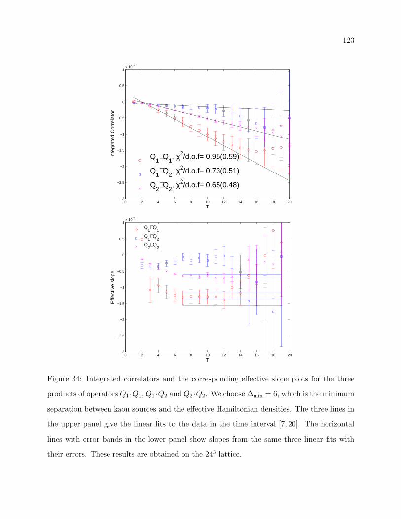
123
0 2 4 6 8 10 12 14 16 18 20−3
−2.5
−2
−1.5
−1
−0.5
0
0.5
1x 10
−3
T
Inte
grat
ed C
orre
lato
r
Q1⋅ Q
1, χ2/d.o.f= 0.95(0.59)
Q1⋅ Q
2, χ2/d.o.f= 0.73(0.51)
Q2⋅ Q
2, χ2/d.o.f= 0.65(0.48)
0 2 4 6 8 10 12 14 16 18 20−3
−2.5
−2
−1.5
−1
−0.5
0
0.5
1x 10
−4
T
Effe
ctiv
e sl
ope
Q
1⋅ Q
1
Q1⋅ Q
2
Q2⋅ Q
2
Figure 34: Integrated correlators and the corresponding effective slope plots for the three
products of operators Q1 ·Q1, Q1 ·Q2 and Q2 ·Q2. We choose ∆min = 6, which is the minimum
separation between kaon sources and the effective Hamiltonian densities. The three lines in
the upper panel give the linear fits to the data in the time interval [7, 20]. The horizontal
lines with error bands in the lower panel show slopes from the same three linear fits with
their errors. These results are obtained on the 243 lattice.

124
2 4 6 8 10 12 14 16 18 20−6
−5
−4
−3
−2
−1
0
1x 10
−3
T
Inte
grat
ed C
orre
lato
r
Q1⋅ Q
1, χ2/d.o.f= 0.53(0.49)
Q1⋅ Q
2, χ2/d.o.f= 1.05(0.70)
Q2⋅ Q
2, χ2/d.o.f= 1.08(0.73)
0 2 4 6 8 10 12 14 16 18 20−3
−2.5
−2
−1.5
−1
−0.5
0
0.5x 10
−4
T
Effe
ctiv
e sl
ope
Q
1⋅ Q
1
Q1⋅ Q
2
Q2⋅ Q
2
Figure 35: Integrated correlators and the corresponding effective slope plots from type 1
diagrams. We choose ∆min = 6, which is the minimum separation between kaon sources and
the effective Hamiltonian densities. The three lines in the upper panel give the linear fits to
the data in the time interval [9, 20]. The horizontal lines with error bands in the lower panel
show slopes from the same three linear fits with their errors. These results are obtained on
the 243 lattice.
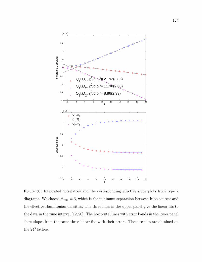
125
2 4 6 8 10 12 14 16 18 20−2
−1.5
−1
−0.5
0
0.5
1
1.5
2x 10
−3
T
Inte
grat
ed C
orre
lato
r
Q1⋅ Q
1, χ2/d.o.f= 21.92(3.85)
Q1⋅ Q
2, χ2/d.o.f= 11.38(2.68)
Q2⋅ Q
2, χ2/d.o.f= 8.86(2.33)
0 2 4 6 8 10 12 14 16 18 20−1.5
−1
−0.5
0
0.5
1
1.5x 10
−4
T
Effe
ctiv
e sl
ope
Q
1⋅ Q
1
Q1⋅ Q
2
Q2⋅ Q
2
Figure 36: Integrated correlators and the corresponding effective slope plots from type 2
diagrams. We choose ∆min = 6, which is the minimum separation between kaon sources and
the effective Hamiltonian densities. The three lines in the upper panel give the linear fits to
the data in the time interval [12, 20]. The horizontal lines with error bands in the lower panel
show slopes from the same three linear fits with their errors. These results are obtained on
the 243 lattice.
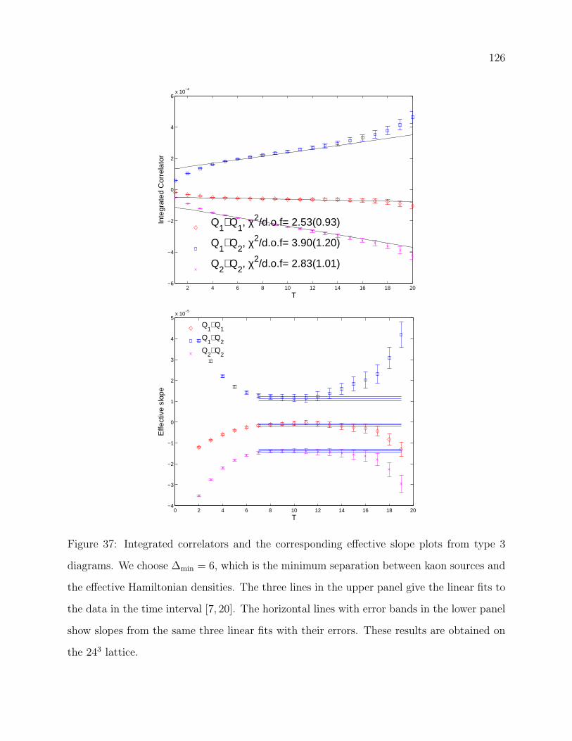
126
2 4 6 8 10 12 14 16 18 20−6
−4
−2
0
2
4
6x 10
−4
T
Inte
grat
ed C
orre
lato
r
Q1⋅ Q
1, χ2/d.o.f= 2.53(0.93)
Q1⋅ Q
2, χ2/d.o.f= 3.90(1.20)
Q2⋅ Q
2, χ2/d.o.f= 2.83(1.01)
0 2 4 6 8 10 12 14 16 18 20−4
−3
−2
−1
0
1
2
3
4
5x 10
−5
T
Effe
ctiv
e sl
ope
Q
1⋅ Q
1
Q1⋅ Q
2
Q2⋅ Q
2
Figure 37: Integrated correlators and the corresponding effective slope plots from type 3
diagrams. We choose ∆min = 6, which is the minimum separation between kaon sources and
the effective Hamiltonian densities. The three lines in the upper panel give the linear fits to
the data in the time interval [7, 20]. The horizontal lines with error bands in the lower panel
show slopes from the same three linear fits with their errors. These results are obtained on
the 243 lattice.
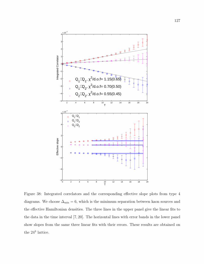
127
2 4 6 8 10 12 14 16 18 20−5
−4
−3
−2
−1
0
1
2
3
4x 10
−3
T
Inte
grat
ed C
orre
lato
r
Q1⋅ Q
1, χ2/d.o.f= 1.15(0.65)
Q1⋅ Q
2, χ2/d.o.f= 0.70(0.50)
Q2⋅ Q
2, χ2/d.o.f= 0.55(0.45)
0 2 4 6 8 10 12 14 16 18 20−6
−4
−2
0
2
4
6x 10
−4
T
Effe
ctiv
e sl
ope
Q
1⋅ Q
1
Q1⋅ Q
2
Q2⋅ Q
2
Figure 38: Integrated correlators and the corresponding effective slope plots from type 4
diagrams. We choose ∆min = 6, which is the minimum separation between kaon sources and
the effective Hamiltonian densities. The three lines in the upper panel give the linear fits to
the data in the time interval [7, 20]. The horizontal lines with error bands in the lower panel
show slopes from the same three linear fits with their errors. These results are obtained on
the 243 lattice.

128
2 4 6 8 10 12 14 16−4.5
−4
−3.5
−3
−2.5
−2
−1.5
−1
−0.5
0
0.5x 10
−3
T
Inte
grat
ed C
orre
lato
r
Q1⋅ Q
1, χ2/d.o.f= 0.55(0.63)
Q1⋅ Q
2, χ2/d.o.f= 0.84(0.82)
Q2⋅ Q
2, χ2/d.o.f= 1.18(0.97)
0 2 4 6 8 10 12 14 16−3
−2.5
−2
−1.5
−1
−0.5
0
0.5x 10
−4
T
Effe
ctiv
e sl
ope
Q
1⋅ Q
1
Q1⋅ Q
2
Q2⋅ Q
2
Figure 39: Integrated correlators and the corresponding effective slope plots from type 1
diagrams. We choose ∆min = 8, which is the minimum separation between kaon sources and
the effective Hamiltonian densities. The three lines in the upper panel give the linear fits to
the data in the time interval [9, 16]. The horizontal lines with error bands in the lower panel
show slopes from the same three linear fits with their errors. These results are obtained on
the 243 lattice.
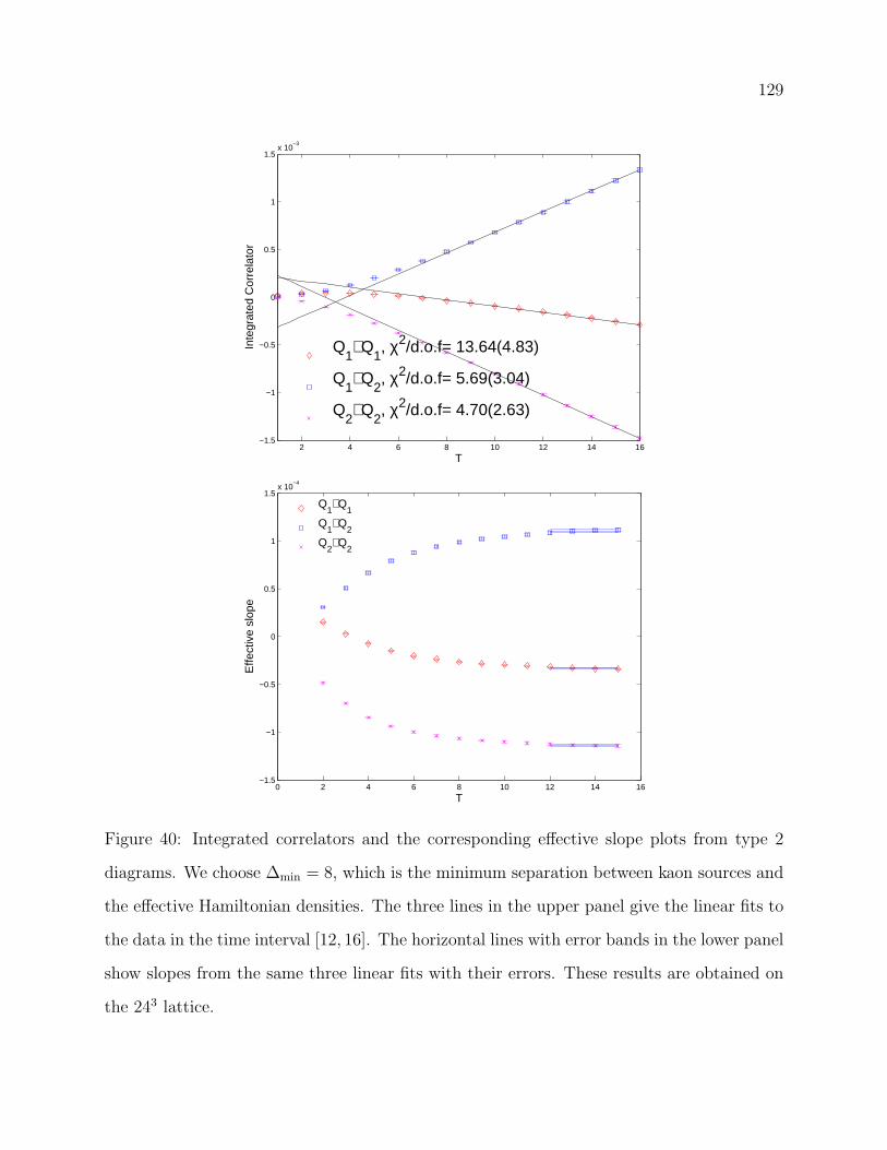
129
2 4 6 8 10 12 14 16−1.5
−1
−0.5
0
0.5
1
1.5x 10
−3
T
Inte
grat
ed C
orre
lato
r
Q1⋅ Q
1, χ2/d.o.f= 13.64(4.83)
Q1⋅ Q
2, χ2/d.o.f= 5.69(3.04)
Q2⋅ Q
2, χ2/d.o.f= 4.70(2.63)
0 2 4 6 8 10 12 14 16−1.5
−1
−0.5
0
0.5
1
1.5x 10
−4
T
Effe
ctiv
e sl
ope
Q
1⋅ Q
1
Q1⋅ Q
2
Q2⋅ Q
2
Figure 40: Integrated correlators and the corresponding effective slope plots from type 2
diagrams. We choose ∆min = 8, which is the minimum separation between kaon sources and
the effective Hamiltonian densities. The three lines in the upper panel give the linear fits to
the data in the time interval [12, 16]. The horizontal lines with error bands in the lower panel
show slopes from the same three linear fits with their errors. These results are obtained on
the 243 lattice.
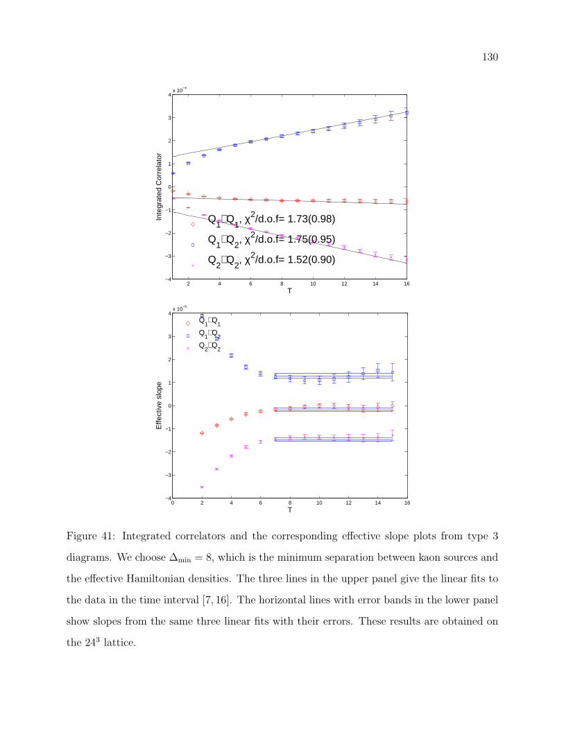
130
2 4 6 8 10 12 14 16−4
−3
−2
−1
0
1
2
3
4x 10
−4
T
Inte
grat
ed C
orre
lato
r
Q1⋅ Q
1, χ2/d.o.f= 1.73(0.98)
Q1⋅ Q
2, χ2/d.o.f= 1.75(0.95)
Q2⋅ Q
2, χ2/d.o.f= 1.52(0.90)
0 2 4 6 8 10 12 14 16−4
−3
−2
−1
0
1
2
3
4x 10
−5
T
Effe
ctiv
e sl
ope
Q
1⋅ Q
1
Q1⋅ Q
2
Q2⋅ Q
2
Figure 41: Integrated correlators and the corresponding effective slope plots from type 3
diagrams. We choose ∆min = 8, which is the minimum separation between kaon sources and
the effective Hamiltonian densities. The three lines in the upper panel give the linear fits to
the data in the time interval [7, 16]. The horizontal lines with error bands in the lower panel
show slopes from the same three linear fits with their errors. These results are obtained on
the 243 lattice.
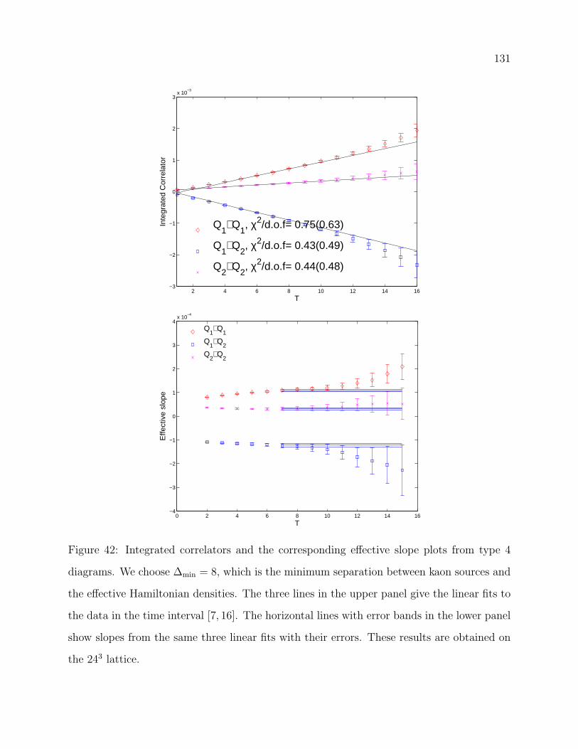
131
2 4 6 8 10 12 14 16−3
−2
−1
0
1
2
3x 10
−3
T
Inte
grat
ed C
orre
lato
r
Q1⋅ Q
1, χ2/d.o.f= 0.75(0.63)
Q1⋅ Q
2, χ2/d.o.f= 0.43(0.49)
Q2⋅ Q
2, χ2/d.o.f= 0.44(0.48)
0 2 4 6 8 10 12 14 16−4
−3
−2
−1
0
1
2
3
4x 10
−4
T
Effe
ctiv
e sl
ope
Q
1⋅ Q
1
Q1⋅ Q
2
Q2⋅ Q
2
Figure 42: Integrated correlators and the corresponding effective slope plots from type 4
diagrams. We choose ∆min = 8, which is the minimum separation between kaon sources and
the effective Hamiltonian densities. The three lines in the upper panel give the linear fits to
the data in the time interval [7, 16]. The horizontal lines with error bands in the lower panel
show slopes from the same three linear fits with their errors. These results are obtained on
the 243 lattice.
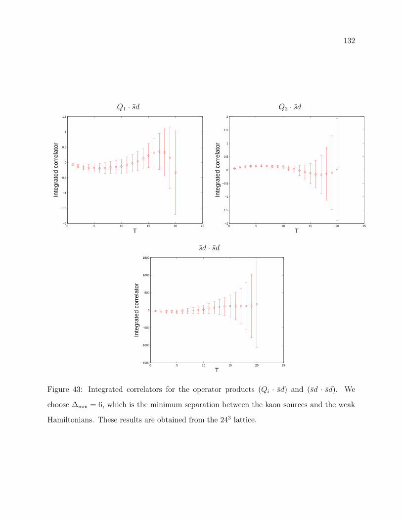
132
Q1 · sd Q2 · sd
0 5 10 15 20 25−2
−1.5
−1
−0.5
0
0.5
1
1.5
T
Inte
grat
ed c
orre
lato
r
0 5 10 15 20 25−2
−1.5
−1
−0.5
0
0.5
1
1.5
2
T
Inte
grat
ed c
orre
lato
r
sd · sd
0 5 10 15 20 25−1500
−1000
−500
0
500
1000
1500
T
Inte
grat
ed c
orre
lato
r
Figure 43: Integrated correlators for the operator products (Qi · sd) and (sd · sd). We
choose ∆min = 6, which is the minimum separation between the kaon sources and the weak
Hamiltonians. These results are obtained from the 243 lattice.
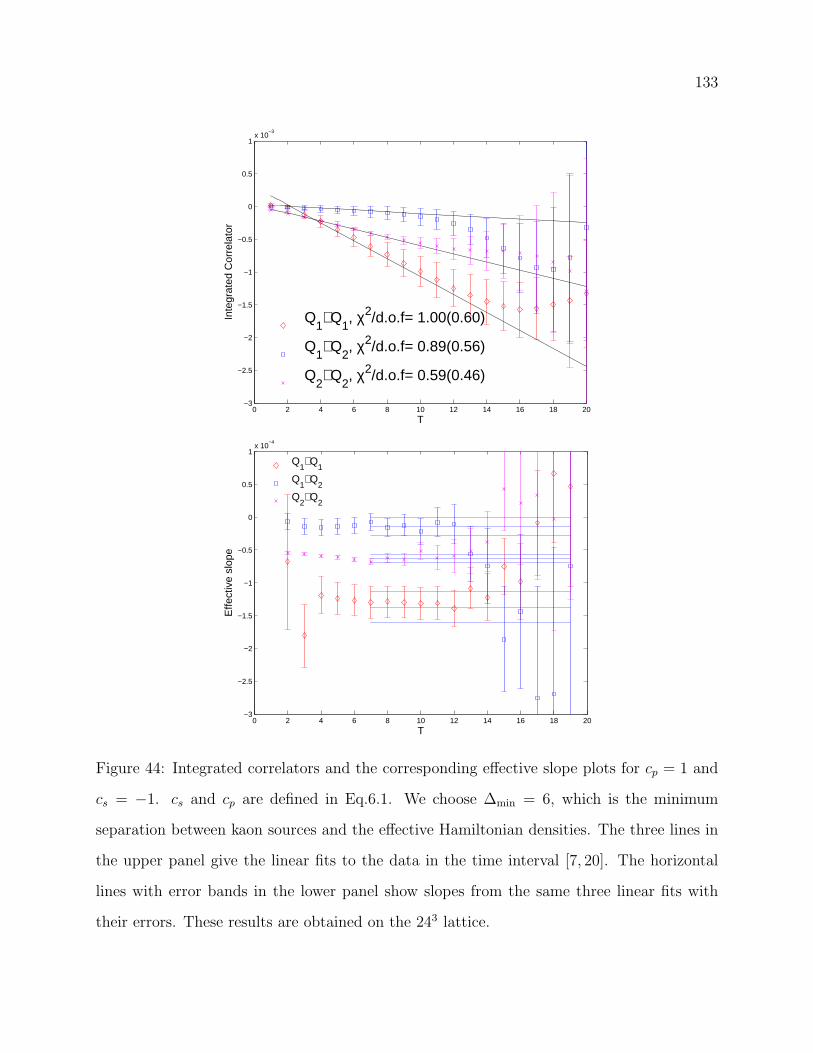
133
0 2 4 6 8 10 12 14 16 18 20−3
−2.5
−2
−1.5
−1
−0.5
0
0.5
1x 10
−3
T
Inte
grat
ed C
orre
lato
r
Q1⋅ Q
1, χ2/d.o.f= 1.00(0.60)
Q1⋅ Q
2, χ2/d.o.f= 0.89(0.56)
Q2⋅ Q
2, χ2/d.o.f= 0.59(0.46)
0 2 4 6 8 10 12 14 16 18 20−3
−2.5
−2
−1.5
−1
−0.5
0
0.5
1x 10
−4
T
Effe
ctiv
e sl
ope
Q
1⋅ Q
1
Q1⋅ Q
2
Q2⋅ Q
2
Figure 44: Integrated correlators and the corresponding effective slope plots for cp = 1 and
cs = −1. cs and cp are defined in Eq.6.1. We choose ∆min = 6, which is the minimum
separation between kaon sources and the effective Hamiltonian densities. The three lines in
the upper panel give the linear fits to the data in the time interval [7, 20]. The horizontal
lines with error bands in the lower panel show slopes from the same three linear fits with
their errors. These results are obtained on the 243 lattice.

134
0 2 4 6 8 10 12 14 16 18 20−3
−2.5
−2
−1.5
−1
−0.5
0
0.5
1x 10
−3
T
Inte
grat
ed C
orre
lato
r
Q1⋅ Q
1, χ2/d.o.f= 0.94(0.59)
Q1⋅ Q
2, χ2/d.o.f= 0.64(0.49)
Q2⋅ Q
2, χ2/d.o.f= 0.85(0.55)
0 2 4 6 8 10 12 14 16 18 20−3
−2.5
−2
−1.5
−1
−0.5
0
0.5
1x 10
−4
T
Effe
ctiv
e sl
ope
Q
1⋅ Q
1
Q1⋅ Q
2
Q2⋅ Q
2
Figure 45: Integrated correlators and the corresponding effective slope plots for cp = 1 and
cs = 1. cs and cp are defined in Eq.6.1. We choose ∆min = 6, which is the minimum
separation between kaon sources and the effective Hamiltonian densities. The three lines in
the upper panel give the linear fits to the data in the time interval [7, 20]. The horizontal
lines with error bands in the lower panel show slopes from the same three linear fits with
their errors. These results are obtained on the 243 lattice.
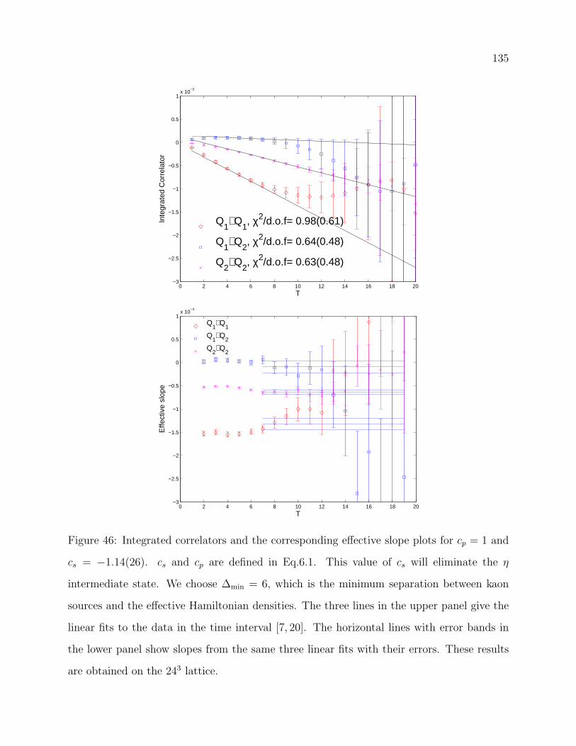
135
0 2 4 6 8 10 12 14 16 18 20−3
−2.5
−2
−1.5
−1
−0.5
0
0.5
1x 10
−3
T
Inte
grat
ed C
orre
lato
r
Q1⋅ Q
1, χ2/d.o.f= 0.98(0.61)
Q1⋅ Q
2, χ2/d.o.f= 0.64(0.48)
Q2⋅ Q
2, χ2/d.o.f= 0.63(0.48)
0 2 4 6 8 10 12 14 16 18 20−3
−2.5
−2
−1.5
−1
−0.5
0
0.5
1x 10
−4
T
Effe
ctiv
e sl
ope
Q
1⋅ Q
1
Q1⋅ Q
2
Q2⋅ Q
2
Figure 46: Integrated correlators and the corresponding effective slope plots for cp = 1 and
cs = −1.14(26). cs and cp are defined in Eq.6.1. This value of cs will eliminate the η
intermediate state. We choose ∆min = 6, which is the minimum separation between kaon
sources and the effective Hamiltonian densities. The three lines in the upper panel give the
linear fits to the data in the time interval [7, 20]. The horizontal lines with error bands in
the lower panel show slopes from the same three linear fits with their errors. These results
are obtained on the 243 lattice.
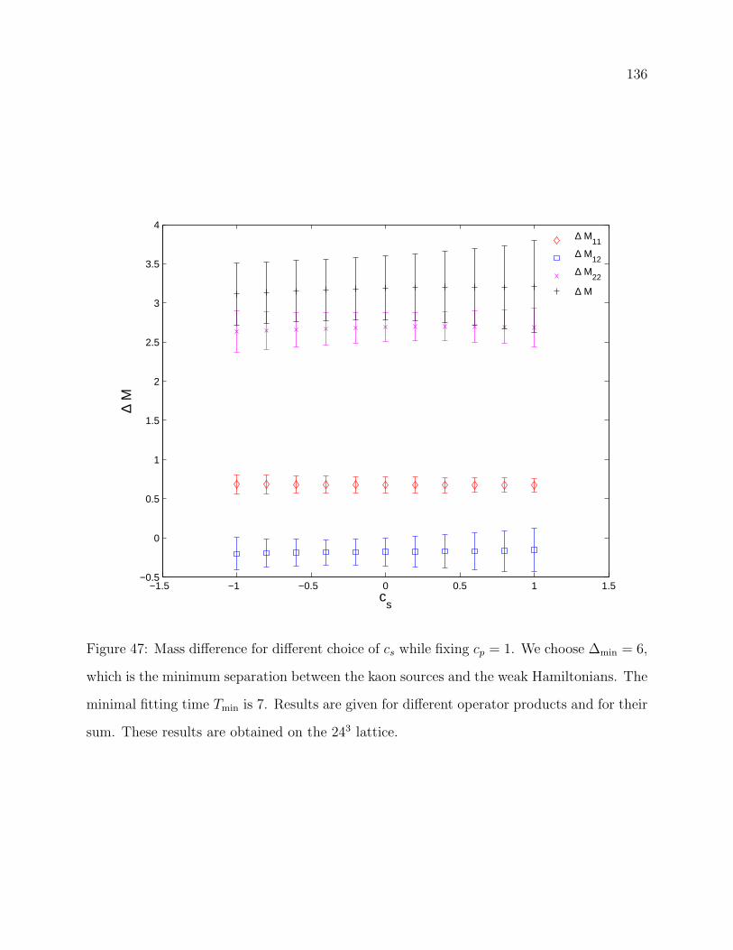
136
−1.5 −1 −0.5 0 0.5 1 1.5−0.5
0
0.5
1
1.5
2
2.5
3
3.5
4
cs
∆ M
∆ M
11
∆ M12
∆ M22
∆ M
Figure 47: Mass difference for different choice of cs while fixing cp = 1. We choose ∆min = 6,
which is the minimum separation between the kaon sources and the weak Hamiltonians. The
minimal fitting time Tmin is 7. Results are given for different operator products and for their
sum. These results are obtained on the 243 lattice.

137
2 4 6 8 10 12 14 16 18 20−0.02
−0.015
−0.01
−0.005
0
0.005
0.01
0.015
0.02
T
Inte
grat
ed C
orre
lato
r
Q1⋅ Q
1, χ2/d.o.f= 0.82(0.91)
Q1⋅ Q
2, χ2/d.o.f= 4.17(2.08)
Q2⋅ Q
2, χ2/d.o.f= 9.54(3.20)
cp = 0, cs = 1, ∆min = 6
1 2 3 4 5 6 7 8 9 10 11 12−3
−2.5
−2
−1.5
−1
−0.5
0
0.5
1
1.5
2x 10
−3
T
Inte
grat
ed C
orre
lato
r
Q1⋅ Q
1, χ2/d.o.f= 0.82(0.91)
Q1⋅ Q
2, χ2/d.o.f= 1.75(1.35)
Q2⋅ Q
2, χ2/d.o.f= 5.37(2.38)
cp = 0, cs = 1, ∆min = 10
Figure 48: Integrated correlator for cp = 0 and cs = 0. We give the results for both ∆min = 6
and ∆min = 10. ∆min is the minimum separation between the kaon sources and the weak
Hamiltonians. All the standard exponentially increasing terms have been removed. The
straight lines give the linear fits to the data in the time interval [7,12]. These results are
obtained on the 243 lattice.
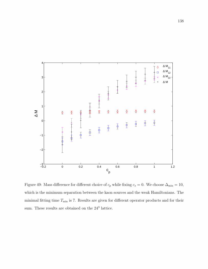
138
−0.2 0 0.2 0.4 0.6 0.8 1 1.2−3
−2
−1
0
1
2
3
4
cp
∆ M
∆ M
11
∆ M12
∆ M22
∆ M
Figure 49: Mass difference for different choice of cp while fixing cs = 0. We choose ∆min = 10,
which is the minimum separation between the kaon sources and the weak Hamiltonians. The
minimal fitting time Tmin is 7. Results are given for different operator products and for their
sum. These results are obtained on the 243 lattice.
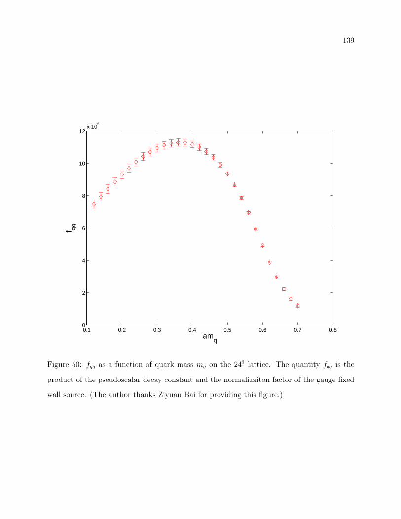
139
0.1 0.2 0.3 0.4 0.5 0.6 0.7 0.80
2
4
6
8
10
12x 10
5
amq
f qq
Figure 50: fqq as a function of quark mass mq on the 243 lattice. The quantity fqq is the
product of the pseudoscalar decay constant and the normalizaiton factor of the gauge fixed
wall source. (The author thanks Ziyuan Bai for providing this figure.)