Embed Size (px)
Citation preview
University of Kentucky University of Kentucky
UKnowledge UKnowledge
Theses and Dissertations--Mechanical Engineering Mechanical Engineering
2016
KINETICS OF MOLTEN METAL CAPILLARY FLOW IN NON-KINETICS OF MOLTEN METAL CAPILLARY FLOW IN NON-
REACTIVE AND REACTIVE SYSTEMS REACTIVE AND REACTIVE SYSTEMS
Hai Fu University of Kentucky, [email protected] Digital Object Identifier: http://dx.doi.org/10.13023/ETD.2016.163
Right click to open a feedback form in a new tab to let us know how this document benefits you. Right click to open a feedback form in a new tab to let us know how this document benefits you.
Recommended Citation Recommended Citation Fu, Hai, "KINETICS OF MOLTEN METAL CAPILLARY FLOW IN NON-REACTIVE AND REACTIVE SYSTEMS" (2016). Theses and Dissertations--Mechanical Engineering. 79. https://uknowledge.uky.edu/me_etds/79
This Doctoral Dissertation is brought to you for free and open access by the Mechanical Engineering at UKnowledge. It has been accepted for inclusion in Theses and Dissertations--Mechanical Engineering by an authorized administrator of UKnowledge. For more information, please contact [email protected].
STUDENT AGREEMENT: STUDENT AGREEMENT:
I represent that my thesis or dissertation and abstract are my original work. Proper attribution
has been given to all outside sources. I understand that I am solely responsible for obtaining
any needed copyright permissions. I have obtained needed written permission statement(s)
from the owner(s) of each third-party copyrighted matter to be included in my work, allowing
electronic distribution (if such use is not permitted by the fair use doctrine) which will be
submitted to UKnowledge as Additional File.
I hereby grant to The University of Kentucky and its agents the irrevocable, non-exclusive, and
royalty-free license to archive and make accessible my work in whole or in part in all forms of
media, now or hereafter known. I agree that the document mentioned above may be made
available immediately for worldwide access unless an embargo applies.
I retain all other ownership rights to the copyright of my work. I also retain the right to use in
future works (such as articles or books) all or part of my work. I understand that I am free to
register the copyright to my work.
REVIEW, APPROVAL AND ACCEPTANCE REVIEW, APPROVAL AND ACCEPTANCE
The document mentioned above has been reviewed and accepted by the student’s advisor, on
behalf of the advisory committee, and by the Director of Graduate Studies (DGS), on behalf of
the program; we verify that this is the final, approved version of the student’s thesis including all
changes required by the advisory committee. The undersigned agree to abide by the statements
above.
Hai Fu, Student
Dr. Dusan P. Sekulic, Major Professor
Dr. Haluk E. Karaca, Director of Graduate Studies
KINETICS OF MOLTEN METAL CAPILLARY FLOW IN NON-REACTIVE AND
REACTIVE SYSTEMS
DISSERTATION
A dissertation submitted in partial fulfillment of the
requirements for the degree of Doctor of Philosophy in the
College of Engineering
at the University of Kentucky
By
Hai Fu
Lexington, Kentucky
Director: Dr. Dusan P. Sekulic, Professor of University of Kentucky
Co-Director: Dr. Kozo Saito, Professor of University of Kentucky
Lexington, Kentucky
2016
Copyright © Hai Fu 2016
ABSTRACT OF DISSERTATION
KINETICS OF MOLTEN METAL CAPILLARY FLOW IN NON-REACTIVE AND
REACTIVE SYSTEMS
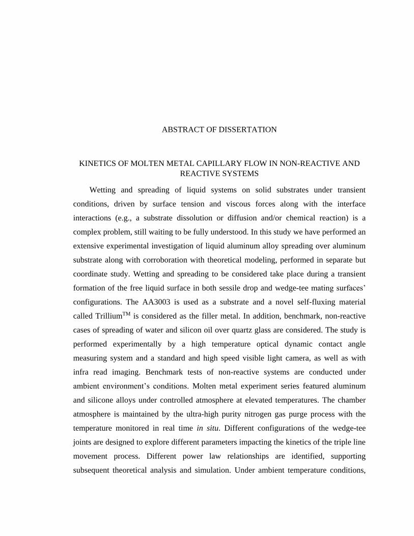
Wetting and spreading of liquid systems on solid substrates under transient
conditions, driven by surface tension and viscous forces along with the interface
interactions (e.g., a substrate dissolution or diffusion and/or chemical reaction) is a
complex problem, still waiting to be fully understood. In this study we have performed an
extensive experimental investigation of liquid aluminum alloy spreading over aluminum
substrate along with corroboration with theoretical modeling, performed in separate but
coordinate study. Wetting and spreading to be considered take place during a transient
formation of the free liquid surface in both sessile drop and wedge-tee mating surfaces’
configurations. The AA3003 is used as a substrate and a novel self-fluxing material
called TrilliumTM is considered as the filler metal. In addition, benchmark, non-reactive
cases of spreading of water and silicon oil over quartz glass are considered. The study is
performed experimentally by a high temperature optical dynamic contact angle
measuring system and a standard and high speed visible light camera, as well as with
infra read imaging. Benchmark tests of non-reactive systems are conducted under
ambient environment’s conditions. Molten metal experiment series featured aluminum
and silicone alloys under controlled atmosphere at elevated temperatures. The chamber
atmosphere is maintained by the ultra-high purity nitrogen gas purge process with the
temperature monitored in real time in situ. Different configurations of the wedge-tee
joints are designed to explore different parameters impacting the kinetics of the triple line
movement process. Different power law relationships are identified, supporting
subsequent theoretical analysis and simulation. Under ambient temperature conditions,
the non-reactive liquid wetting and spreading experiments (water and oil systems) were
studied to verify the equilibrium triple line location relationships. The kinetics
relationship between the dynamic contact angle and the triple line location is identified.
Additional simulation and theoretical analysis of the triple line movement is conducted
using the commercial computer software platform Comsol in a collaboration with a team
from Washington State University within the NSF sponsored Grant #1235759 and #
1234581. The experimental work conducted here has been complemented by a
verification of the Comsol phase-field modeling. Both segments of work (experimental
and numerical) are parts of the collaborative NSF sponsored project involving the
University of Kentucky and Washington State University. The phase field modeling used
in this work was developed at the Washington State University and data are corroborated
with experimental results obtained within the scope of this Thesis.
KEYWORDS: Kinetics, Wetting and Spreading, Wedge-tee, TrilliumTM, Model
Hai Fu
Apr. 15th, 2016
KINETICS OF MOLTEN METAL CAPILLARY FLOW IN NON-REACTIVE AND
REACTIVE SYSTEMS
By
Hai Fu
Dr. Dusan P. Sekulic
Director of Dissertation
Dr. Kozo Saito
Co-Director of Dissertation
Dr.Haluk E. Karaca
Director of Graduate Studies
Apr. 15th, 2016

DEDICATION
DEDICATED TO MY PARENTS FOR SUPPORTING ME OVER THE YEARS
UNCONDITIONALLY AND KENNETH TUBAUGH FOR STANDING BY MY SIDE
THROUGH IT ALL
iii
ACKNOWLEDGEMENTS
This dissertation and my PhD research work over the years were funded by
multiple NSF projects. I want to thank my advisor Professor Dusan P. Sekulic for his
generosity, resourceful insight and most of all, his kind support and encouragement. I
would never have been able to finish my dissertation without his guidance and help. My
deepest gratitude goes to Professor Dusan P. Sekulic for accepting me as his student
when time was the hardest for me. The excellent research atmosphere in the ISM Brazing,
Soldering and Heat Exchangers Research Laboratory will always be one of the best
memories in my life.
I would like to thank my committee members, Dr. Kozo Saito, Dr. Y-T Cheng, Dr.
Tianxiang Li and Dr. John Young, for their guidance and time during the defense process.
Special thanks goes to Dr. Michael Winter for being willing for participating in my final
defense committee at the last moment.
Many thanks to Dr. Mikhail Krivilev, Dr. Sinisa Mesarovic and Mohammad
Dehsara for the continuous cooperation research in the NSF project. And many thanks to
Dr. Fazleena Badurdeen, Dr. Robert Gregory, Dr. Margaret Schroder, Dr. Leslie Vincent,
Dr. Gregory Luhan and Adam Brown for making the NSF funded course work a
wonderful experience. Thanks to Dr. Doug Hawksworth and Daniel Busbaher for their
support in the research work. Thanks to Dr. Haluk E. Karaca and his students Sayed M.
Saghaian and Ali Turabi for allowing me to use his lab facilities to conduct several
experiments. Thanks to Mechanical Engineering Department staff members, Charles
Arvin, Heather-Michele Adkins, Peter Hayman and Steven Adkins, for their help and
support during my PhD study.
Finally, I would like to thank my parents for being my parents with love and
support no matter what. And I would like to thank Kenneth Tubaugh for being there for
me through thick and thin.
iv
TABLE OF CONTENTS
ACKNOWLEDGEMENTS ............................................................................................................ iii
LIST OF TABLES ......................................................................................................................... vii
LIST OF FIGURES ...................................................................................................................... viii
CHAPTER 1: INTRODUCTION ................................................................................................... 1
1.1 Background Fundamentals ..................................................................................................... 1
1.2 Scope of the research ............................................................................................................. 4
1.3 Organization of the dissertation ............................................................................................. 5
CHAPTER 2: LITERATURE REVIEW ........................................................................................ 7
2.1 Overview ................................................................................................................................ 7
2.2 Wetting and spreading ........................................................................................................... 8
2.2.1 The Concept of Contact Angle........................................................................................ 8
2.2.2 Dynamic contact angle .................................................................................................... 9
2.2.3 Triple line location (TLL) ............................................................................................. 11
2.2.4 Surface energy and Young’s equation .......................................................................... 11
2.2.5 Capillary number, capillary length and Bond number .................................................. 12
2.3 Experimental evidence of non-reactive wetting and spreading ........................................... 13
2.3.1 Sessile drop experiments ............................................................................................... 14
2.3.2 Capillary displacement experiments ............................................................................. 15
2.3.3 Wilhelmy plate balance experiments ............................................................................ 16
2.3.4 Tilting plate experiments .............................................................................................. 19
2.3.5 Capillary bridge experiments ........................................................................................ 20
2.4 Non-reactive wetting kinetics models .................................................................................. 20
2.4.1 Hoffman-Voinov-Tanner law ....................................................................................... 21
2.4.2 Jiang’s Correlation Model ............................................................................................. 22
2.4.3 Bracke’s Correlation Model .......................................................................................... 23
2.4.4 Seebergh’s Correlation Model ...................................................................................... 24
2.4.5 Blake’s Molecular Model ............................................................................................. 25
2.5 Near-reactive (molten metal) case: CAB Technology description ...................................... 26
2.5.1 Sessile drop experiment ................................................................................................ 31
2.5.2 Wetting balance experiment.......................................................................................... 35
2.5.3 Optical hot stage microscopy ........................................................................................ 38
v
2.6 Wetting kinetics theories and models at elevated temperatures ........................................... 40
2.6.1 Diffusion-controlled wetting of metal/ceramic systems model .................................... 43
2.6.2 Dissolutive wetting model ............................................................................................ 44
CHAPTER 3: BENCHMARK STUDY OF THE KINETICS ON A CAPILLARY FLOW OF
NON-REACTIVE LIQUID SYSTEMS ........................................................................................ 47
3.1 Overview .............................................................................................................................. 47
3.2 Experimental setup and procedure ....................................................................................... 48
3.2.1 Material preparation ...................................................................................................... 48
3.2.2 Experiment configuration ............................................................................................. 52
3.2.3 Experiment procedures ................................................................................................. 54
3.3 Experiment results and discussion ....................................................................................... 61
3.3.1 Validation of the equilibrium relationship between the contact angle and the triple line
location ................................................................................................................................... 61
3.3.2 Dynamic contact angle experimental correlation .......................................................... 67
3.3.3 Kinetics of two liquid systems ...................................................................................... 73
3.4 Summary .............................................................................................................................. 82
CHAPTER 4: EXPERIMENTAL EQUIPMENT AND PROCEDURES FOR THE HIGH
TEMPERATURE CAPILLARY FLOW STUDY ........................................................................ 84
4.1 Overview .............................................................................................................................. 84
4.2 Experiment Configuration ................................................................................................... 85
4.3 Sample preparation .............................................................................................................. 90
4.3.1 Wedge-tee type of sample preparation .......................................................................... 91
4.3.2 Sessile drop sample preparation (non-wetting case) ..................................................... 96
4.4 Experiment procedures ...................................................................................................... 100
4.4.1 Wedge-tee configuration and sessile drop experiment ............................................... 100
4.4.2 OCA furnace FLIR infrared camera temperature phenomenology ............................. 104
4.5 Summary ............................................................................................................................ 107
CHAPTER 5: WETTING OF MOLTEN CLAD METAL ON WETTED AND NON-WETTED
SURFACES ................................................................................................................................109
5.1 Overview ............................................................................................................................ 109
5.2 Experimental study of the molten clad metal at elevated temperatures ............................. 110
5.2.1 Molten clad metal wetting on the wetting surface – preliminary tests ........................ 110
5.2.2 Molten clad metal surface tension review ................................................................... 113
5.3 Analysis of the sessile drop triple line region .................................................................... 115
vi
5.4 Summary ............................................................................................................................ 121
CHAPTER 6: WEDGE-TEE CONFIGURATION KINETICS OF THE CAPILLARY FLOW OF
MOLTEN CLAD ......................................................................................................................... 123
6.1 Overview ............................................................................................................................ 123
6.2 Experimental study of the molten clad metal spreading kinetics in a wedge-tee
configuration at elevated temperatures .................................................................................... 124
6.2.1 Molten clad metal kinetics study methodology .......................................................... 124
6.2.2 Molten clad metal kinetics under deteriorated background atmosphere ..................... 133
6.2.3 Molten clad metal kinetics with different clad layer thicknesses ............................... 136
6.2.4 Molten clad metal kinetics on non-wetting surface .................................................... 141
6.3 Phase-field model analysis of the molten clad metal kinetics ............................................ 145
6.4 Summary ............................................................................................................................ 146
CHAPTER 7: CONCLUSION AND FUTURE WORK ............................................................ 148
7.1 Main conclusions from the current study ........................................................................... 148
7.2 Future work ........................................................................................................................ 151
APPENDICES ............................................................................................................................. 153
Appendix A .............................................................................................................................. 153
Appendix B .............................................................................................................................. 160
Appendix C .............................................................................................................................. 166
Appendix D .............................................................................................................................. 171
Appendix E .............................................................................................................................. 173
REFERENCES ............................................................................................................................ 181
VITA ............................................................................................................................................ 192
vii
LIST OF TABLES
Table 3.1 Properties of Liquids ......................................................................................... 49
Table 3.2 Thermo Scientific, #2950-001 microscope glass surface roughness
measurement data.............................................................................................................. 51
Table 3.3 Different initial thicknesses of water layer data ............................................... 59
Table 3.4 Different initial thicknesses of silicone oil layer data ....................................... 59
Table 4.1 Surface roughness of AA3003 .......................................................................... 95
Table 4.2 Surface roughness of alumina ......................................................................... 100
Table 5.1 Contact angle measurement results of wetting surface ................................... 113
Table 5.2 Chemical composition for different points in the triple line (refer to Fig. 5.6)
......................................................................................................................................... 118
viii
LIST OF FIGURES
Fig. 2.1 Contact angle concept schematics ......................................................................... 9
Fig. 2.2 Advancing contact angle (left) and receding contact angle (right) comparison .. 10
Fig. 2.3 Triple line location schematics ............................................................................ 11
Fig. 2.4 Force balance of the three-phase contact line ...................................................... 12
Fig. 2.5 Capillary displacement measurement of apparent contact angle (Kistler, 1993) 15
Fig. 2.6 Wilhelmy plate configuration .............................................................................. 17
Fig. 2.7 Plunge tank configuration (Kistler, 1993) ........................................................... 18
Fig. 2.8 Tilting plate method configuration ...................................................................... 19
Fig. 2.9 (a) Comparison between empirical correlations and Hoffman’s data for 𝐶𝑎 >
10 − 3 (Seebergh et al., 1992), (b) Comparison between Seeburgh’s model and all
the low capillary number data (Seebergh et al., 1992) .............................................. 25
Fig. 2.10 Transparent high temperature CAB laboratory furnace system ........................ 28
Fig. 2.11 CAB continuous production line (SECO/WARWICK GROUP,
http://www.secowarwick.com/en/products/cab-controlled-atmosphere-brazing-
furnaces/ (accessed on Sept.5th, 2015)) .................................................................... 29
Fig. 2.12 Schematic of composite-clad brazing sheet (TrilliumTM) brazing process ........ 31
Fig. 2.13 Schematic of the profiles as the solid cube melts to wet and spread during the
sessile drop experiment .............................................................................................. 32
Fig. 2.14 Methods of sessile drop experiments: (a) traditional method, (b) in situ
formation of the alloy, (c) dispensed drop, (d) transferred drop, (e) double substrate,
(f) tilted plate (Eustathopoulos et al., 1999) .............................................................. 33
Fig. 2.15 Sessile drop experiment setup schematic diagram for the boron nitride and
molten aluminum system (Fujii et al., 1993) ............................................................. 34
Fig. 2.16 Sessile drop experiment setup schematic diagram for aluminum wetting on
sapphire (Weirauch et al., 1990) ................................................................................ 34
Fig. 2.17 Schematic diagram of the wetting balance experiment (Rivollet et al., 1990) .. 36
Fig. 2.18 Schematic diagram of meniscus formed with the immersed vertical plate for (a)
wetting and (b) non-wetting liquid ............................................................................ 37
Fig. 2.19 Leitz hot stage 1750 (Thorsen et al., 1984) ....................................................... 38
Fig. 2.20 Linkam THMS 600 hot stage system (Zhao et al., 2009).................................. 39
Fig. 2.21 Linkam THMS 600 hot stage installed on an Oplympus BX51M optical
microscopy system ..................................................................................................... 39
Fig. 2.22 Schematic diagram of interaction mechanism for Al-Mg alloy droplet on SiC
substrate (Candan et al., 2011) .................................................................................. 42
Fig. 2.23 Schematic representation of Al-Mg alloy droplet final contact angle 𝜃𝐹 on
reactive substrate compared to unreactive substrate contact angle 𝜃0 (Dezellus et al.,
2010) .......................................................................................................................... 42
ix
Fig. 2.24 Schematic diagram of the sessile drop final contact angle with relationship to
the upper and lower liquid contact angles (Warren et al., 1998) ............................... 45
Fig. 3.1 Glass slides Wilhelmy plate configuration with the fixed horizontal plate and
moving vertical plate ................................................................................................. 49
Fig. 3.2 3D scanning image of topography of Thermo Scientific, #2950-001 microscope
glass, measured by Zygo New View TM 7300 3D Optical Surface Profiler, (from
blue to red color, the level increases) ........................................................................ 50
Fig. 3.3 3D scanning intensity map of topography of Thermo Scientific, #2950-001
microscope glass, measured by Zygo New View TM 7300 3D Optical Surface
Profiler ....................................................................................................................... 50
Fig. 3.4 Schematic diagram of the non-reactive liquid kinetics experiment configuration
................................................................................................................................... 53
Fig. 3.5 (a) Wedge-tee glass slides configuration (Wilhelmy plate configuration) and (b)
triple line location on both left side (Yl) and right side (Yr) ..................................... 53
Fig. 3.6 Water meniscus formation process profile .......................................................... 56
Fig. 3.7 Screenshot of Image-Pro© tracking object measurement method ....................... 57
Fig. 3.8 Experimental water meniscus growth lengths profiles in 9 time frames ............. 58
Fig. 3.9 Experimental water meniscus growth lengths profiles in 5 time frames ............. 58
Fig. 3.10 Silicone oil meniscus formation process profile................................................ 60
Fig. 3.11 Meniscus triple line location height and contact angle ...................................... 61
Fig. 3.12 Water layer thickness and vertical distance relationship with error bars
comparison ................................................................................................................. 62
Fig. 3.13 Theoretical prediction and experimental comparison of the contact angle and
triple line location relationship in water on glass system .......................................... 63
Fig. 3.14 Silicone oil layer thickness and vertical distance relationship with error bars
comparison ................................................................................................................. 64
Fig. 3.15 Theoretical prediction and experimental comparison of the contact angle and
triple line location relationship in silicone oil on glass system ................................. 65
Fig. 3.16 Water and silicone oil systems comparison of theoretical prediction with
experiment data for contact angle and triple line location correlation ...................... 66
Fig. 3.17 Experiment and empirical correlation comparison of dynamic contact angle and
capillary number relationship for silicone oil system in linear scale ......................... 69
Fig. 3.18 Schematic screenshot of the initial dynamic contact angle 𝜃𝐷1 and the last
dynamic contact angle 𝜃𝐷𝑛 in Wilhelmy plate configuration ................................... 69
Fig. 3.19 Silicone oil dynamic contact angle correlation models and experimental data
comparison in log-log scale ....................................................................................... 70
Fig. 3.20 Water dynamic contact angle correlation models and experimental data
comparison in log-log scale ....................................................................................... 71
Fig. 3.21 Modified empirical correlation and water on glass system experiment data
comparison ................................................................................................................. 72
x
Fig. 3.22 Averaged water and silicone oil systems triple line kinetics comparison with
error bars .................................................................................................................... 73
Fig. 3.23 Silicone oil and water scaled time kinetics ........................................................ 75
Fig. 3.24 Linear scale of silicone oil and water kinetics with triple line location and
dynamic contact angle ............................................................................................... 76
Fig. 3.25 (a) Silicone oil triple line location dynamics experimental data and Washburn
theoretical prediction and (b) water triple line location dynamics experimental data
and Washburn theoretical prediction ......................................................................... 78
Fig. 3.26 Triple line location kinetics for silicone oil (a) and water (b) in log-log scales 80
Fig. 3.27 Silicone oil and water triple line kinetics comparison with error bars in log scale
................................................................................................................................... 81
Fig. 4.1 High temperature contact angle measurement system’s schematic diagram ...... 86
Fig. 4.2 OCA system facility ............................................................................................ 87
Fig. 4.3 Operation screenshot of SCA20 software ........................................................... 89
Fig. 4.4 Temperature settings screenshot of SCA20 software .......................................... 89
Fig. 4.5 Wedge-tee sample 3-D configuration of 0.03 thickness TrilliumTM clad metal .. 91
Fig. 4.6 XY plane view of wedge-tee sample configuration of 0.03 thickness TrilliumTM
clad metal ................................................................................................................... 92
Fig. 4.7 Configuration of the vertical piece and clad substrate ........................................ 93
Fig. 4.8 (a) The surface topography of the AA3003 substrate measured by Hitachi S-
3200-N Scanning Electron Microscope; (b) 3D scanning image of topography of
AA3003 substrate measured by Zygo New View TM 7300 3D Optical Surface
Profiler; (c) Brazing sheet cross section structure (horizontal mating surface, Fig. 4.5)
................................................................................................................................... 95
Fig. 4.9 Aluminum alloy spreading test samples. (a) 0.03 mm thickness TrilliumTM clad
configuration, (b) 0.4 mm thickness Trillium configuration ..................................... 96
Fig. 4.10 The surface topography of the alumina substrate scanned by Hitachi S-3200-N
Scanning Electron Microscope .................................................................................. 97
Fig. 4.11 The surface topography of the alumina substrate measured by Hitachi S-3200-N
Scanning Electron Microscope for EDS analysis area .............................................. 98
Fig. 4.12 Alumina substrate area spectra from Fig. 4.11 .................................................. 98
Fig. 4.13 3D scanning image of topography of alumina substrate measured by Zygo New
View TM 7300 3D Optical Surface Profiler; (b) 3D scanning intensity map of
topography of alumina substrate measured by Zygo New View TM 7300 3D Optical
Surface Profiler .......................................................................................................... 99
Fig. 4.14 (a) Joint domain configuration and (b) vertical/horizontal length of the joint 101
Fig. 4.15 A selection of image sequences decomposed from a recorded movie indicating
the evolution of joint formation with time (0.03mm thickness TrilliumTM of
experiment 091212) ................................................................................................. 102
Fig. 4.16 Tracking objects method (experiment 091212) ............................................... 103
xi
Fig. 4.17 ImageJ low-bond axisymmetric drop shape analysis sample .......................... 104
Fig. 4.18 Dummy sample configuration ......................................................................... 105
Fig. 4.19 Infrared camera setup in the OCA system ....................................................... 106
Fig. 4.20 IR Image of the temperature distribution of the wedge-tee joint formation .... 106
Fig. 4.21 Symmetric temperature distribution of the wedge-tee joint region ................. 107
Fig. 5.1 Temperature profile of the sessile drop in the experiment of the wetting surface
................................................................................................................................. 111
Fig. 5.2 A snake-based approach to the measurement of the contact angle ................... 112
Fig. 5.3 TrilliumTM surface tension experimental result comparison ............................. 115
Fig. 5.4 Non-wetting sessile drop triple line region on alumina ..................................... 116
Fig. 5.5 Non-wetting sessile drop triple line region on alumina ..................................... 116
Fig. 5.6 SEM image of non-wetting sessile drop triple line region ................................ 117
Fig. 5.7 Chemical composition at different locations in the triple line region .............. 118
Fig. 5.8 Wetting of the molten clad metal sessile drop triple line on AA3003 .............. 120
Fig. 5.9 Zoomed-in image of wetting of the molten clad metal sessile drop triple line on
AA3003 .................................................................................................................... 121
Fig. 6.1 Wedge-tee configuration of TrilliumTM clad metal with various thicknesses on
wetting substrate of AA3003: (a) 0.03 mm thickness TrilliumTM clad; (b) 0.4 mm
thickness TrilliumTM foil-formed filler; (c) 0.8 mm thickness TrilliumTM foil-formed
filler .......................................................................................................................... 125
Fig. 6.2 Temperature profiles for joint formation process with recordings of every 10
seconds (experiment 102612) .................................................................................. 127
Fig. 6.3 Oxygen level in the joint formation process (experiment 102612) ................... 127
Fig. 6.4 Schematic diagram of triple line location at wedge-tee joint area with molten clad
metal ........................................................................................................................ 128
Fig. 6.5 A sequence of images decomposed from a recorded movie indicating the
evolution of the joint meniscus formation as a function of time (0.03mm thickness
TrilliumTM) (Test 091212) ....................................................................................... 129
Fig. 6.6 (a) Normalized spreading distance in both horizontal (X) and vertical (Y)
directions and (b) normalized spreading distance in y direction with standard error
bars, (an average of 7 times repeated experiment of the 0.03 mm thickness
TrilliumTM clad metal) ............................................................................................. 131
Fig. 6.7 Triple line location kinetics plot in two stages .................................................. 132
Fig. 6.8 Joint formation cross-section after re-solidification image ............................... 133
Fig. 6.9 Triple line kinetics of the joint formation with different oxygen concentration
levels ........................................................................................................................ 135
Fig. 6.10 Normalized triple line kinetics of the joint formation with different oxygen
concentration levels ................................................................................................. 135
Fig. 6.11 0.4 mm thickness TrilliumTM kinetics study sample configuration ................. 137
xii
Fig. 6.12 Linear scale representation of 0.4mm thickness TrilliumTM clad metal kinetics
with triple line location and dynamic contact angle (Fu et al., 2016) ..................... 137
Fig. 6.13 Log scale of (i) silicone oil, (ii) water, (iii) 0.03 mm thickness TrilliumTM and
(iv) 0.4 mm thickness TrilliumTM kinetics comparison with Washburn’s equation, Eq.
3.10 i.e., the power law correlations ........................................................................ 138
Fig. 6.14 Linear scale of 0.03 mm thickness TrilliumTM, 0.4 mm thickness TrilliumTM and
0.8 mm thickness TrilliumTM kinetics comparison .................................................. 140
Fig. 6.15 Log scale of 0.03 mm thickness TrilliumTM, 0.4 mm thickness TrilliumTM and
0.8 mm thickness TrilliumTM kinetics comparison .................................................. 141
Fig. 6.16 TrilliumTM filler metal on non-wetting alumina horizontal surface configuration
with thicker filler metal of 0.8mm ........................................................................... 142
Fig. 6.17 Molten clad metal spreading on vertical AA3003 plate with non-wetting
horizontal surface (Experiment 05052015) ............................................................. 142
Fig. 6.18 Kinetics of 0.03 mm thickness TrilliumTM, 0.4 mm thickness TrilliumTM, 0.8
mm thickness TrilliumTM, all on wetting horizontal surface, and 0.8 mm thickness
TrilliumTM on non-wetting horizontal but wetting vertical ..................................... 143
Fig. 6.19 Kinetics of 0.03 mm thickness TrilliumTM, 0.4 mm thickness TrilliumTM, 0.8
mm thickness TrilliumTM and 0.8 mm thickness TrilliumTM on non-wetting
horizontal substrate but wetting vertical substrate ................................................... 144
Fig. 6.20 The comparison between experimental data and phase field modeling .......... 146
1
CHAPTER 1: INTRODUCTION
1.1 Background Fundamentals
Surface tension driven flow has been studied both theoretically and experimentally for a
long time (de Gennes, 1985; Voinov, 1976; Dussan, 1979.; Kistler, 1993; Eustathopoulos
et al., 1999; Quéré, 2008; Bonn et al., 2009; Sui et al., 2014). The surface interactions
play important role in many technologies. These include but are not restricted to oil
recovery, pesticides deposition, water drainage, industrial cooling of reactors, etc. The
associated phenomena manifest themselves at multiple scales, in microfluidics, nano-
printing, coating technology, etc. Hence, they play an important role in almost every
aspect of our lives, and are of key importance for many applications (Bonn et al., 2009).
Although the surface driven flow has been studied for a long time, only a limited number
of high temperature studies were published before 1940s (Eustathopoulos et al. 1999). A
new wave of wetting studies started to come out in the 1980s in the studies of metal
joining, non-similar materials bonding, especially ceramic brazing and glazing (de
Gennes, 1985; Eustathopoulos et al., 1999). In high temperature metal bonding, governed
by the interfacial interactions, multiple parameters are relevant. These include
constitutive species of the system, temperature, pressure, surface topography, background
atmosphere, reaction processes, electric charges and gravity impact, among the others
less dominant. The associated very complex phenomena are crucial to understanding of
the structure, strength and durability of the bonded materials (Zhao et al., 2006; Busbaher
et al., 2010).
2
In the brazing process, the materials involved are heated to temperatures above the filler
metal melting temperature hence turning a solid metal into a liquid, forming the high
temperature flow over the mating surfaces. Spreading of the liquid requires capillary
action (Schwartz, 2003). The metallurgical bond is ultimately formed after solidification
of the filler metal. The temperatures involved in brazing are, according to a widely
adopted convention (Sekulic, 2013) above 450°C (liquidus temperature above 450°C but
below the solidus temperature of the bonding metals, Schwartz, 2003).
In automotive industry and many aerospace applications, aluminum is normally preferred
for its superior physical and economical properties over, say, copper. Motivated by these
applications, this work focusses on aluminum alloy both used as mating surfaces
substrates and filler metals. Associated materials processing require stringent processing
conditions, including the liquid phase, imposed by novel designs of the components of
engineering systems in those applications (Sekulic, 2011).
The kinetics of the molten metal flow has a direct impact on the solidified metal
properties, notably strength and durability. The liquid metal wetting assumes often
chemically inert atmosphere (as well as in a limit vacuum). Due to a high sensitivity in
reaction of the involved materials, in particular at the elevated temperatures, formation of
oxides is present. (Eustathopoulos et al. 1999). The oxide film formed during the process
has to be eliminated to allow the free flow of the molten metal around the joint areas. For
example, for high production rate joining of automobile heat exchanger assemblies, the
Controlled Atmosphere Brazing (CAB) became the state-of-the-art manufacturing
process (Sekulic, 2013). Furthermore, in various aerospace applications, vacuum brazing
is a standard process. The low moisture level and drastically reduced oxygen level are
3
benefits of the desired atmosphere filled with inert gas (or vacuum) to ensure the
controllable minimal oxidation layer formation on the surfaces of the metal. In controlled
atmosphere traditionally, the molten metal at elevated temperatures is covered with a flux
coating, so that the flux can react to disrupt the oxide film. Analogously, addition of a
getter (Mg) in vacuum brazing serves a similar supporting role. Under this circumstance,
the flux reaction at the elevated temperature in the controlled atmosphere can disrupt the
aluminum oxide layer and provide the free flow of the molten metal, driven into the joint
by the capillary force.
Recently, a novel aluminum alloy, TrilliumTM (US Patent US20100206529), was
introduced. Trillium features the potassium fluoroaluminate flux imbedded into the solid
filler (Hawksworth et al., 2012; Fu et al., 2013; Yu et al., 2013; Sekulic, 2013). This
“fluxless” brazing (actually an absence of the flux coating) achieves the same or better
results than the traditional brazing with a flux, and decreases the complexity and
expenses at the same time (Sekulic, 2013). In this dissertation, the kinetics of the joint
formation involving this material is the subject of this study.
It is well understood that the kinetics of the wetting process is controlled by factors like
temperature, atmosphere composition, surface properties, reaction rates, in addition to the
materials systems properties. Controlling different variables to study the kinetics process
helps better understand of the brazing process, hence getting ultimately a better quality of
brazing. The interest of the study is to analyze and understand the kinetics of the wetting
processes in brazing aluminum. Both, reactive (molten aluminum on aluminum) and non-
reactive systems (water and silicon oil on glass) were considered.
4
1.2 Scope of the research
Wetting and spreading of liquid systems on solid substrates under transient conditions,
driven by surface tension and retarded by viscosity, under both non-reactive and reactive
conditions at liquid/solid interface are being investigated. The study was performed
experimentally and is supported by theoretical modeling simultaneously developed by a
collaborating team. Wetting and spreading to be considered takes place during a transient
formation of the free liquid surface in a so called wedge-tee configuration, using AA3003
metal as a substrate. In addition, non-reactive benchmark cases of spreading of water and
silicon oil over quartz glass as a substrate were considered. Measurements were obtained
by using a high temperature optical dynamic contact angle measuring system equipped by
both low and high speed visible light and infra-red cameras. Benchmark tests of non-
reactive systems were be conducted under ambient environment’s conditions. In a high
temperature reactive (or more precisely, a weak-reactive) molten metal liquid experiment
series, aluminum and silicone alloys were used. The atmosphere was controlled by the
ultra-high purity nitrogen gas purge process with the temperature monitored in real time
in situ. Different configurations of the wedge-tee joints are designed to explore the
different parameters impacting the kinetics of the triple line movement process. Power
law relationships are identified in the experiments, supporting the subsequent theoretical
analysis and simulation. The set of non-reactive liquid wetting and spreading experiments
has been performed at the ambient temperatures. Water and silicon oil systems were
studied to verify the contact angles equilibrium triple line location relationships. The
kinetics between the dynamic contact angle and the triple line location relation was
5
identified. An empirical best fit model was determined for benchmarking the high
temperature reactive wetting and spreading tests.
Additional simulation and theoretical analysis of the triple line movement prediction
were performed.
The main objectives of the study were to explore, explain, model and ultimately
understand the dynamics of the wetting process in both reactive and non-reactive systems
and at both high and low temperatures. The main research hypothesis of the experimental
work is that a novel liquid metal (Al-Si eutectic + KxFyAlz) spreading kinetics, driven by
surface tension, can be modeled by a Washburn type correlation (power law), regardless
of the reactive nature of the solid-liquid substrate.
1.3 Organization of the dissertation
Following the introduction in Chapter 1, Chapter 2 reviews the literature involving the
fundamental knowledge and most recent research related to the non-reactive, and reactive
surface tension driven wetting and spreading on smooth surfaces. High temperature
wetting, especially in brazing will also be reviewed.
As a benchmark study, the capillary flow of the non-reactive liquid systems is studied
experimentally. Two material systems: water and silicone oil are considered in Chapter 3.
Chapter 4 introduces the high temperature brazing experimental facility, namely the
Optical Contact Angle analyzer (OCA), as well as specific procedures that were adopted
for different experiments for the near reactive surface driven capillary molten metal flow
on different wetting surfaces.
6
Chapter 5 explores the weak-reactive surface driven capillary flow of the molten metal on
the wetting surface. The specific wedge-tee joint configuration, topographically similar to
the non-reactive experiment configuration, is introduced in the experiments to study the
reaction impacted triple line kinetics. Different power law relationships have been
discovered in different stages of the process.
A similar configuration of wedge-tee joint with a non-wetting horizontal surface is
presented in Chapter 6 to further explore the reactive capillary flow kinetics of the molten
metal. The method of surface tension measurement of the molten metal on the non-
wetting surface is also introduced in this chapter.
Conclusion and further discussion of the results are presented in Chapter 7, with future
research objectives as well as existing problems presented in the last chapter.
In the Appendices section, Appendix A discusses the error analysis from the benchmark
experiments. Appendix B extends the molten clad metal wetting on the non-wetting
surface with the measurement of surface tension of the molten clad metal. Appendix C
gives the review of aluminum alloy surface tension in the known literature to compare
with the measured molten clad metal surface tension. Appendix D quantifies the
meniscus curvature of the wedge-tee joint area from molten clad metal. Appendix E
includes the phase field model discussion, physical parameters, phase field model
parameters and the steps to determine the parameters.
7
CHAPTER 2: LITERATURE REVIEW
2.1 Overview
Related research on the scope of this dissertation is reviewed in this chapter. A broader
view of the wetting phenomenon in general is discussed here.
The literature is grouped into two parts. The first part summarizes the research on the
non-reactive surface tension driven flow at low temperatures, including the brief
presentation of fundamental theories of the wetting and spreading. The approach to the
basic experimental methods for the study of wetting and spreading is addressed. Different
theoretical models for the non-reactive spreading are presented in this part. The second
part of the literature review provides the controlled atmosphere brazing optical contact
angle analyzer furnace description used for design of the high temperature experimental
methods for surface tension driven flow. The text offers a review of relevant studies on
surface tension driven flow at elevated temperatures for reactive flows. Finally, the
aluminum brazing process related joint formation featuring interaction between the filler
metal and substrate is covered in this part as well. The introduction of some fundamental
concepts in this review is not intended to be either complete or rigorous. Such reviews are
available (De Gennes, 1985) and would not be repeated here. Rather, only key concept
relevant for this study will be summarized.
8
2.2 Wetting and spreading
Wetting phenomenon is one of the basic physical phenomena in nature. As stated by de
Gennes (1985), the wetting of a solid is based on physical chemistry which involves the
concept of wettability, including the interpretation of surface forces as van der Waals
forces and fluid dynamics. Spreading of a liquid is the ultimate result of wetting of the
liquid (Myers, 1999). Wetting and spreading implies an involvement of chemistry,
physics and engineering insights (Bonn et al., 2009). The surface chemistry is the key
factor influencing the wetting and spreading phenomena (Bonn et al., 2009). Along with
surface chemistry, surface forces like van der Waals and electrostatic forces are also
controlling the wetting and spreading phenomena in general (Bonn et al., 2009).
Application of wetting and spreading are numerous and span from painting, lubrication,
dye and printing up to oil industry, power generation, biochemical deposition of
pesticides, skin care, etc. In recent years, wetting and spreading phenomena applications
in designing super hydrophobic surfaces has triggered an increasing interest, leading to
such applications as self-cleaning, nanofluidics, and electro-wetting (Yuan et al., 2013).
2.2.1 The Concept of Contact Angle
Contact angle is one of the major physical entities in any study of wetting and spreading
processes. It represents a quantitative measure of the wetting process. When a drop of
liquid contacts a solid surface, the liquid either spreads more or less unconstraint across
the surface to form a thin film, or spreads to a limited extent to form a drop (e.g., sessile
drop) on the surface (Myers, 1999). Contact angle as a wetting metric indicates the
degree of wetting. For example, it is well known that if the contact angle, say θ, is larger
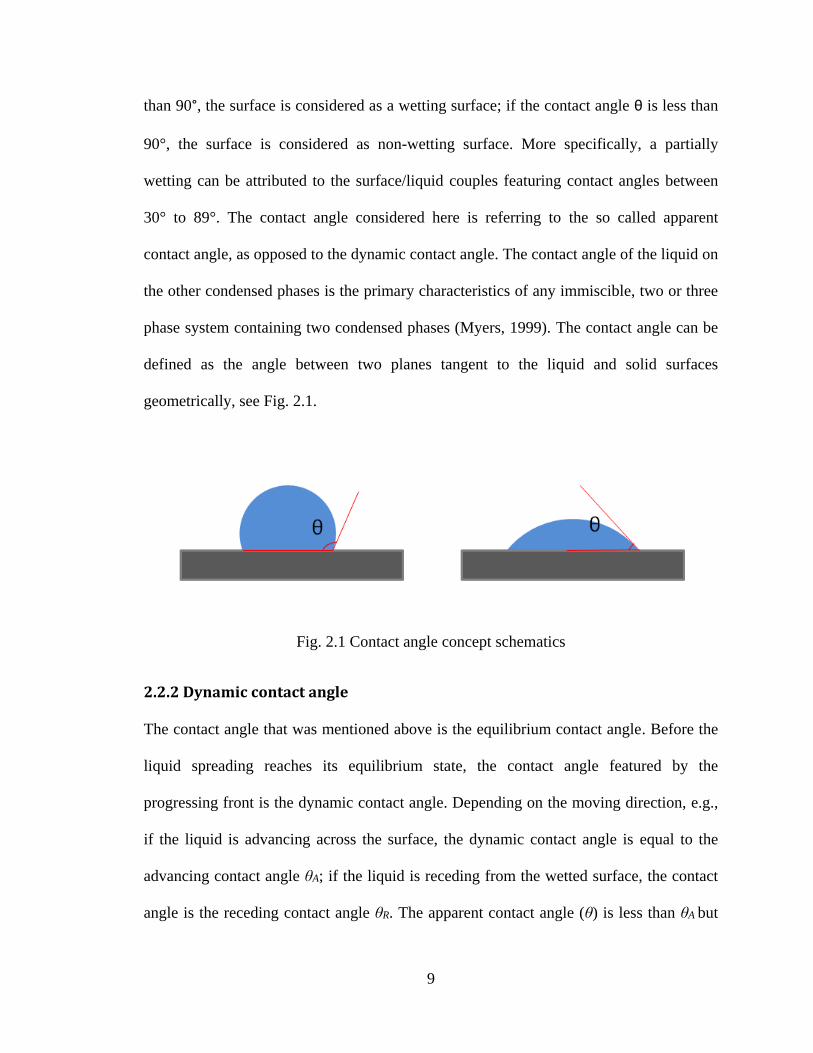
9
than 90°, the surface is considered as a wetting surface; if the contact angle θ is less than
90°, the surface is considered as non-wetting surface. More specifically, a partially
wetting can be attributed to the surface/liquid couples featuring contact angles between
30° to 89°. The contact angle considered here is referring to the so called apparent
contact angle, as opposed to the dynamic contact angle. The contact angle of the liquid on
the other condensed phases is the primary characteristics of any immiscible, two or three
phase system containing two condensed phases (Myers, 1999). The contact angle can be
defined as the angle between two planes tangent to the liquid and solid surfaces
geometrically, see Fig. 2.1.
Fig. 2.1 Contact angle concept schematics
2.2.2 Dynamic contact angle
The contact angle that was mentioned above is the equilibrium contact angle. Before the
liquid spreading reaches its equilibrium state, the contact angle featured by the
progressing front is the dynamic contact angle. Depending on the moving direction, e.g.,
if the liquid is advancing across the surface, the dynamic contact angle is equal to the
advancing contact angle θA; if the liquid is receding from the wetted surface, the contact
angle is the receding contact angle θR. The apparent contact angle (θ) is less than θA but
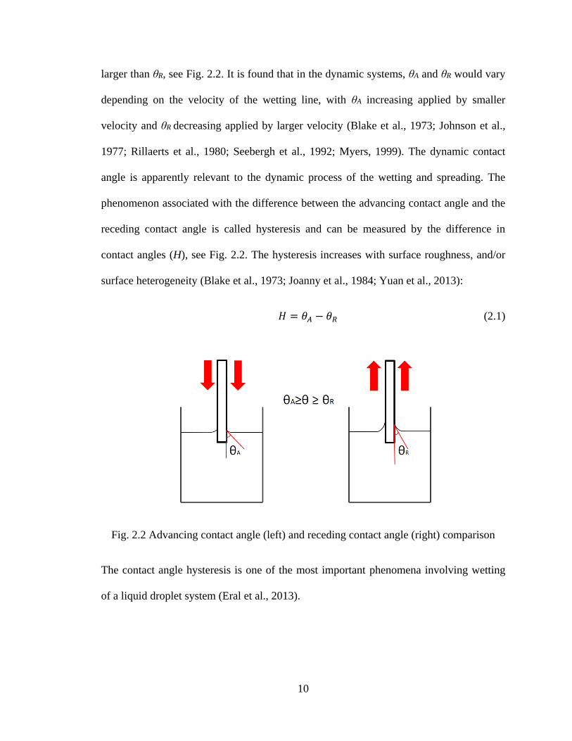
10
larger than θR, see Fig. 2.2. It is found that in the dynamic systems, θA and θR would vary
depending on the velocity of the wetting line, with θA increasing applied by smaller
velocity and θR decreasing applied by larger velocity (Blake et al., 1973; Johnson et al.,
1977; Rillaerts et al., 1980; Seebergh et al., 1992; Myers, 1999). The dynamic contact
angle is apparently relevant to the dynamic process of the wetting and spreading. The
phenomenon associated with the difference between the advancing contact angle and the
receding contact angle is called hysteresis and can be measured by the difference in
contact angles (H), see Fig. 2.2. The hysteresis increases with surface roughness, and/or
surface heterogeneity (Blake et al., 1973; Joanny et al., 1984; Yuan et al., 2013):
𝐻 = 𝜃𝐴 − 𝜃𝑅 (2.1)
Fig. 2.2 Advancing contact angle (left) and receding contact angle (right) comparison
The contact angle hysteresis is one of the most important phenomena involving wetting
of a liquid droplet system (Eral et al., 2013).
11
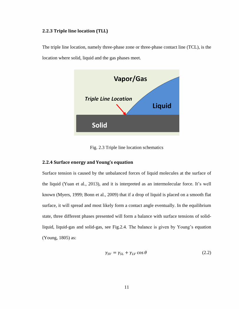
2.2.3 Triple line location (TLL)
The triple line location, namely three-phase zone or three-phase contact line (TCL), is the
location where solid, liquid and the gas phases meet.
Fig. 2.3 Triple line location schematics
2.2.4 Surface energy and Young’s equation
Surface tension is caused by the unbalanced forces of liquid molecules at the surface of
the liquid (Yuan et al., 2013), and it is interpreted as an intermolecular force. It’s well
known (Myers, 1999; Bonn et al., 2009) that if a drop of liquid is placed on a smooth flat
surface, it will spread and most likely form a contact angle eventually. In the equilibrium
state, three different phases presented will form a balance with surface tensions of solid-
liquid, liquid-gas and solid-gas, see Fig.2.4. The balance is given by Young’s equation
(Young, 1805) as:
𝛾𝑆𝑉 = 𝛾𝑆𝐿 + 𝛾𝐿𝑉 cos 𝜃 (2.2)
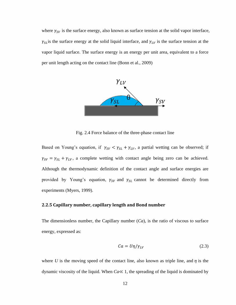
12
where 𝛾𝑆𝑉 is the surface energy, also known as surface tension at the solid vapor interface,
𝛾𝑆𝐿is the surface energy at the solid liquid interface, and 𝛾𝐿𝑉 is the surface tension at the
vapor liquid surface. The surface energy is an energy per unit area, equivalent to a force
per unit length acting on the contact line (Bonn et al., 2009)
Fig. 2.4 Force balance of the three-phase contact line
Based on Young’s equation, if 𝛾𝑆𝑉 < 𝛾𝑆𝐿 + 𝛾𝐿𝑉, a partial wetting can be observed; if
𝛾𝑆𝑉 = 𝛾𝑆𝐿 + 𝛾𝐿𝑉 , a complete wetting with contact angle being zero can be achieved.
Although the thermodynamic definition of the contact angle and surface energies are
provided by Young’s equation, 𝛾𝑆𝑉 and 𝛾𝑆𝐿 cannot be determined directly from
experiments (Myers, 1999).
2.2.5 Capillary number, capillary length and Bond number
The dimensionless number, the Capillary number (Ca), is the ratio of viscous to surface
energy, expressed as:
𝐶𝑎 = 𝑈𝜂/𝛾𝐿𝑉 (2.3)
where U is the moving speed of the contact line, also known as triple line, and 𝜂 is the
dynamic viscosity of the liquid. When Ca≪ 1, the spreading of the liquid is dominated by
13
the surface tension rather than the viscous effects. Bonn et al. (2009) shows that, in that
case, 𝐶𝑎 ≈ 10−5 − 10−3. Capillary length, however, is the ratio of surface tension to
gravitational force, expressed as:
𝑙𝑐 = √𝛾𝐿𝑉/𝜌𝑔 (2.4)
Note that when the drop radius is smaller than the capillary length, gravity can be
neglected (Bonn et al., 2009).
Another dimensionless number to measure the importance of surface tension and the
body force is known as Bond number or Eötvös number (𝐵𝑜 =∆𝜌𝑔𝐿2
𝛾𝐿𝑉, where ∆𝜌 is the
two phases of liquid or gas density difference, L is is the characteristic length) (Hager,
2012).
2.3 Experimental evidence of non-reactive wetting and spreading
The dynamics of the surface driven flow has been studied for over a century and much of
the study was focused mostly on ambient temperature and non-reactive liquid systems.
Back in the early 20th century, by using capillary tube of uniform internal circular cross-
section throughout, Washburn (1921) has studied the kinetics of capillary flow of
mercury, water and oil systems, and presented the Washburn type of flow with liquid
penetration distance obeying the square root relationship to time. Compared to the
spontaneous, natural wetting and spreading, for the forced wetting, the apparent dynamic
contact angle has been the focus of the research (Kistler, 1993). The distinction between
the two will be explained below, see Section 2.3.2. Common experimental methods for
the forced wetting case include sessile drop configuration and the capillary displacement
14
configuration (Washburn, 1921; Tanner, 1979; Šikalo et al., 2005; Han et al., 2014), and
Wilhelmy plate configuration or wetting-balance method (Johnson et al., 1977; Ström et
al., 1990). The contact angles can be directly measurement as the tangent angle at the
triple line contact point by a contact angle goniometer (Yuan et al., 2013). Alternately,
they may be determined by a measurement of the tangent angle at the triple line contact
point from the extracted images from a video camera (Han et al., 2014). The liquid
systems in the studies mostly involve, as mentioned earlier, water, mercury, oils and
organic chemical compounds. Based on the experimental data, the dynamic contact angle
𝜃𝐷can be correlated with the triple line movement kinetics, mostly represented by the
capillary number Ca (Kistler, 1993).
2.3.1 Sessile drop experiments
One of the most common experimental studies of the surface tension driven flow is the
sessile drop setup, see Fig.2.1. In this type of setup, the liquid drop is placed on a
horizontal surface, so that the drop can spread over the surface due to the surface tension
force. Different roughness of the surfaces can be used in these tests to study the surface
topography impact on the spreading. The dynamic contact angle, equilibrium contact
angle and the triple line movement can all be recorded. There are many studies regarding
this form of testing with different liquid systems (Schwartz et al., 1972; Tanner, 1979;
Hocking et al., 1982; Biance et al., 2004; Lee et al., 2011). The dominating force
presented on the spreading is an inertial force and the surface tension during the dynamic
phase of the process. The drops can be generated by a syringe, either with/without the
automatic dispenser (Yuan et al., 2013). A microscope with either CMOS camera, CCD
camera or high speed camera is used to record the images of the spreading process, so
15
that the contact angles and triple line movement can be measured through an image of a
drop’s profile, interpreted as the cross-section region of the sessile drop. Such tests are
mostly done at ambient temperature, under constant pressure.
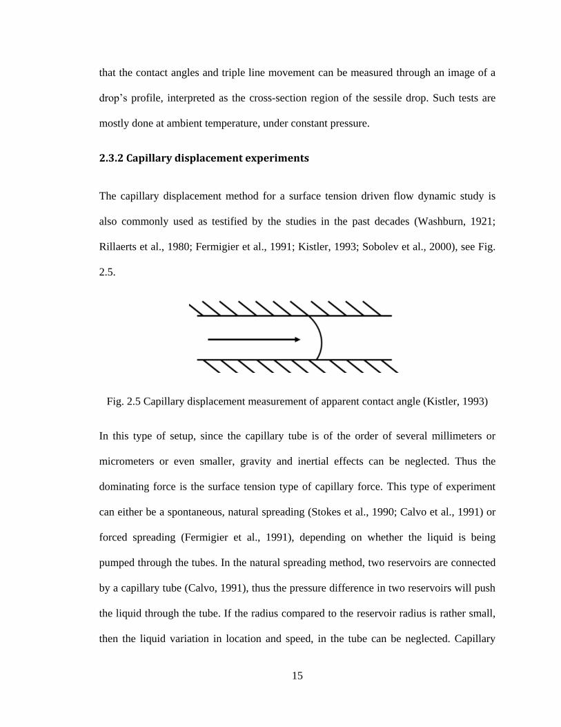
2.3.2 Capillary displacement experiments
The capillary displacement method for a surface tension driven flow dynamic study is
also commonly used as testified by the studies in the past decades (Washburn, 1921;
Rillaerts et al., 1980; Fermigier et al., 1991; Kistler, 1993; Sobolev et al., 2000), see Fig.
2.5.
Fig. 2.5 Capillary displacement measurement of apparent contact angle (Kistler, 1993)
In this type of setup, since the capillary tube is of the order of several millimeters or
micrometers or even smaller, gravity and inertial effects can be neglected. Thus the
dominating force is the surface tension type of capillary force. This type of experiment
can either be a spontaneous, natural spreading (Stokes et al., 1990; Calvo et al., 1991) or
forced spreading (Fermigier et al., 1991), depending on whether the liquid is being
pumped through the tubes. In the natural spreading method, two reservoirs are connected
by a capillary tube (Calvo, 1991), thus the pressure difference in two reservoirs will push
the liquid through the tube. If the radius compared to the reservoir radius is rather small,
then the liquid variation in location and speed, in the tube can be neglected. Capillary
16
displacement experiments are similar to the sessile drop experiments in a way that the
microscope with camera and liquid dispenser with syringe can also be used. If the
spreading is a forced spreading, then pumps can be used to pump liquid through the
capillary tubing. With the aid of microscope and camera, the images of each action in the
spreading process can be recorded, thus the contact angles and the triple line movement
can be measured.
According to Washburn (1921), for the vertical capillaries, the capillary spontaneous
natural rise, h, can be calculated as:
ℎ =2𝛾𝐿𝑉 cos 𝜃
∆𝜌𝑔𝑟 (2.5)
where r is the capillary radius, 𝑔 is the gravitational acceleration, ∆𝜌 is the density
difference between liquid and vapor, 𝜃 is the equilibrium contact angle, and 𝛾𝐿𝑉 is the
surface tension between liquid and vapor.
For the horizontal capillaries, a similar correlation can be found as:
𝑙2 =𝑟𝑡𝛾𝐿𝑉 cos 𝜃
2𝜂 (2.6)
where 𝑙 is the capillary distance, 𝑟 is capillary radius, 𝜂 is the liquid viscosity, 𝜃 is the
equilibrium contact angle, 𝛾𝐿𝑉 is the surface tension between liquid and vapor, and 𝑡 is
the time required for the capillary intrusion.
2.3.3 Wilhelmy plate balance experiments
In the forced spreading experiments, the Wilhelmy plate configuration (Wilhelmy, 1863)
is very common , see Fig. 2.2 and Fig.2.6.
17
Fig. 2.6 Wilhelmy plate configuration
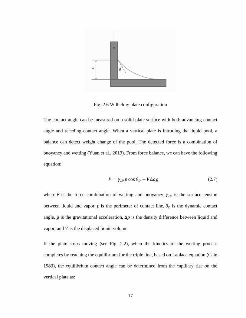
The contact angle can be measured on a solid plate surface with both advancing contact
angle and receding contact angle. When a vertical plate is intruding the liquid pool, a
balance can detect weight change of the pool. The detected force is a combination of
buoyancy and wetting (Yuan et al., 2013). From force balance, we can have the following
equation:
𝐹 = 𝛾𝐿𝑉𝑝 cos 𝜃𝐷 − 𝑉∆𝜌𝑔 (2.7)
where 𝐹 is the force combination of wetting and buoyancy, 𝛾𝐿𝑉 is the surface tension
between liquid and vapor, 𝑝 is the perimeter of contact line, 𝜃𝐷 is the dynamic contact
angle, 𝑔 is the gravitational acceleration, ∆𝜌 is the density difference between liquid and
vapor, and 𝑉 is the displaced liquid volume.
If the plate stops moving (see Fig. 2.2), when the kinetics of the wetting process
completes by reaching the equilibrium for the triple line, based on Laplace equation (Cain,
1983), the equilibrium contact angle can be determined from the capillary rise on the
vertical plate as:
18
𝑠𝑖𝑛 𝜃 = 1 −∆𝜌𝑔𝑦2
2𝛾𝐿𝑉 (2.8)
where 𝜃 is the equilibrium contact angle, 𝑔 is the gravitational acceleration, ∆𝜌 is the
density difference of the liquid and vapor, 𝑦 is the capillary rise height, 𝛾𝐿𝑉 is the surface
tension between liquid and vapor.
The Wilhelmy plate balance method is a fairly accurate method widely used to determine
the dynamic contact angle and the relationship between the dynamic contact angle and
the wetting speeds. It should be noted that a sufficient quantity of liquid should be used to
avoid the impact of the liquid level change approaching the equilibrium.
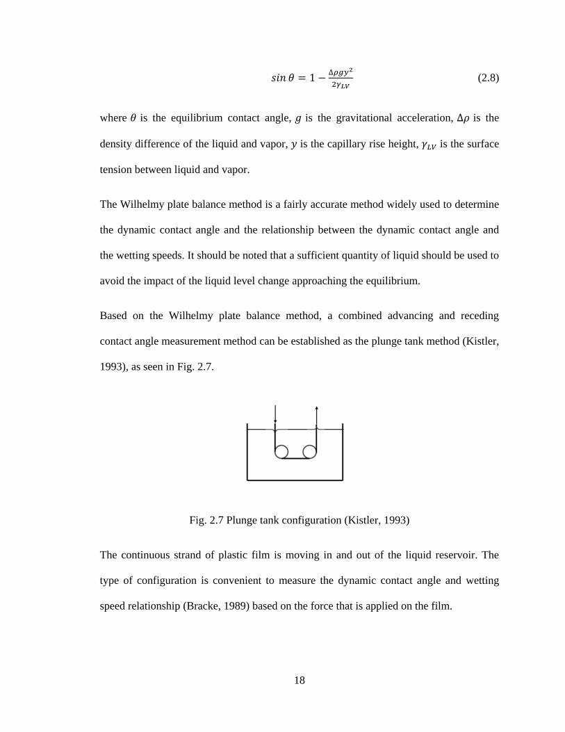
Based on the Wilhelmy plate balance method, a combined advancing and receding
contact angle measurement method can be established as the plunge tank method (Kistler,
1993), as seen in Fig. 2.7.
Fig. 2.7 Plunge tank configuration (Kistler, 1993)
The continuous strand of plastic film is moving in and out of the liquid reservoir. The
type of configuration is convenient to measure the dynamic contact angle and wetting
speed relationship (Bracke, 1989) based on the force that is applied on the film.
19
2.3.4 Tilting plate experiments
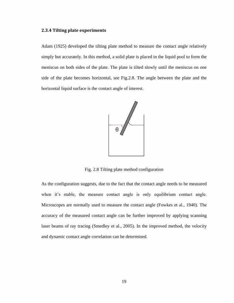
Adam (1925) developed the tilting plate method to measure the contact angle relatively
simply but accurately. In this method, a solid plate is placed in the liquid pool to form the
meniscus on both sides of the plate. The plate is tilted slowly until the meniscus on one
side of the plate becomes horizontal, see Fig.2.8. The angle between the plate and the
horizontal liquid surface is the contact angle of interest.
Fig. 2.8 Tilting plate method configuration
As the configuration suggests, due to the fact that the contact angle needs to be measured
when it’s stable, the measure contact angle is only equilibrium contact angle.
Microscopes are normally used to measure the contact angle (Fowkes et al., 1940). The
accuracy of the measured contact angle can be further improved by applying scanning
laser beams of ray tracing (Smedley et al., 2005). In the improved method, the velocity
and dynamic contact angle correlation can be determined.
20
2.3.5 Capillary bridge experiments
Vagharchakian et al. (2008) and Restagno et al. (2009) developed the capillary bridge
method to measure the contact angle. In this method, a transparent convex surface (such
as a watch glass) with a radius of curvature R of a few centimeters is used on a liquid
bath with test liquid. The meniscus forms at the contact line around the curvature of the
spherical surface. By measuring the changes of the wetted area and the distance between
the surface and the liquid, the dynamic contact angle can be determined based on
Young’s equation. The capillary bridge method offers the way to measure both advancing
and receding contact angle with precise results (Vagharchakian et al., 2008; Retsgno et al.,
2009). However, due to the high sensitivity of the method, liquid evaporation may
impose negative impact on the accuracy of the results.
2.4 Non-reactive wetting kinetics models
The kinetics of the liquid spreading has been studied over the past decades, as
emphasized in the opening sections of this chapter. It is suggested (Kistler, 1993) based
on dimensional analysis that the dynamic contact angle, 𝜃𝐷, should be related to the
contact angle, 𝜃, capillary number, Weber number We (𝑊𝑒 =𝜌𝑈2𝐿𝑐
𝛾, 𝐿𝑐 is characteristic
length), Bond number Bo (𝐵𝑜 =∆𝜌𝑔𝐿𝑐
2
𝛾 ), viscosity ratio, density ratio, species L, and
surface properties (such as roughness 𝜀, porosity 𝜉 and electric charges 𝜒).
𝜃𝐷 = 𝑓 (𝜃, 𝐶𝑎, 𝑊𝑒, 𝐵𝑜,𝜇2
𝜇1,
𝜌2
𝜌1,
𝐿𝑖
𝐿, 𝜀, 𝜉, 𝜒) (2.9)
21
Two different approaches to the wetting modeling the kinetics of spreading on a solid
surface deserve our attention. One is the hydrodynamic model (Seebergh et al., 1992).
Let us assume, based on the scaling implied by Eq. (2.9), that the surface tension and
viscosity are the dominant forces. The other approach is the molecular-kinetic model,
focusing on the behavior/interactions of liquid and the solid molecules (Eral et al., 2013).
In the hydrodynamic models, an important variable is the wetting velocity U, (Hoffman
et al., 1975). Also, wetting is characterized by the contact angle. The variation of the
contact angle with respect to time or wetting velocity reflects the kinetics of the wetting
process.
Most of the kinetics models are based on the correlation between contact angle, dynamic
contact angle and the wetting velocity. As shown in Eq. (2.3), wetting velocity can also
be represented by the capillary number relationship, as 𝐶𝑎 = 𝑈𝜂/𝛾𝐿𝑉 . Washburn (1921)
developed the correlations of triple line movement kinetics, see Eq. (2.5) and Eq. (2.6). In
the 70s, Hoffman et al. (1975), Voinov et al. (1976) and Tanner (1979) have presented
the Hoffman-Voinov-Tanner law, describing the empirical correlation between contact
angles and wetting velocity. Later experiments have verified this correlation in different
forms, such as Jiang’s model (Jiang et al., 1979), Bracke’s model (Bracke et al., 1989),
Seebergh’s model (Seebergh et al., 1992), etc.
2.4.1 Hoffman-Voinov-Tanner law
Hoffman (1975) first brought up the correlation between the experimental data by
plotting the contact angle and the capillary number for low capillary numbers, measured
via capillary displacement measurement. 5 different liquids were used in his experiment.
22
It should be noted that the kinetics process is dominated by the interfacial and viscous
forces. Voinov (1976) also demonstrated that for a small Reynolds number, there is a
dependence of the contact angle on wetting velocity. It wasn’t until Tanner (1979) who
derived the 𝜃𝐷~𝐶𝑎1/3 power law hydrodynamic theory correlation based on his
experiments. The correlation, Hoffman-Voinov-Tanner Law, has been formulated as
follows.
𝜃𝐷3 − 𝜃3 = 𝑐𝑇𝐶𝑎 (2.10)
Where cT is a constant based on the solid-vapor-liquid selection, 𝜃𝐷is the dynamic contact
angle, and 𝜃 is the equilibrium contact angle. In order to apply the law correctly, the
capillary number has to be much smaller than 1, and 𝜃𝐷 ≤ 135°. It also has be noted that
the liquids tested in this interpretation are the oil-based liquids, such as silicone oil. The
correlation between dynamic contact angle and the capillary number is independent of the
measurement configuration (Kisler, 1993).
2.4.2 Jiang’s Correlation Model
Based on Hoffman et al. (1975) experiment data, the fitting correlation between contact
angle and the capillary number was presented by Jiang et al. (1979), Eq. (2.11). The
correlation was also applied to other systems, Schwartz et al. (1970).
𝑐𝑜𝑠 𝜃 −𝑐𝑜𝑠 𝜃𝐷
𝑐𝑜𝑠 𝜃+1= 𝑡𝑎𝑛ℎ(4.96𝐶𝑎0.702) (2.11)
It should be noted the Jiang’s correlation model is a different form of Hoffman-Voinov-
Tanner Law, with the dominant forces being still surface tension and viscosity. The
23
correlation was verified with other sources of experiment data, as long as 𝐵𝑜 < 10−1
and 𝑊𝑒 < 10−3where
𝐵𝑜 =𝜌𝑔𝐿1
𝛾𝐿𝑉 (2.12)
𝑊𝑒 =𝜌𝑈2𝐿
𝛾𝐿𝑉 (2.13)
The Bond number, Bo, is the ratio of gravity to interfacial forces, and the Weber number,
We, is the ratio of inertial forces to interfacial forces at the liquid-gas interface; L is the
characteristic length, U is the wetting velocity. Based on the empirical results, it is
known that if inertia and gravity are negligible, Jiang’s correlation model would be valid
for different liquid-gas-solid systems.
2.4.3 Bracke’s Correlation Model
Based on his own experiment data, Bracke et al. (1989) obtained the equation as follows.
𝑐𝑜𝑠 𝜃 −𝑐𝑜𝑠 𝜃𝐷
𝑐𝑜𝑠 𝜃+1= 2𝐶𝑎0.5 (2.14)
The Wilhelmy plate configuration was used in Bracke’s experiment to obtain the date of
𝜃𝐷 and U. The correlation model was also verified with other experiments data source
from different measurement configurations with different organic liquid systems. Bracke
confirms Eq. (2.14) as well as Eq. (2.10) is comparable for small capillary numbers. It is
also presented that the correlation is applicable for clean and dry plates as the rate of
wetting is much faster for the prewetted plate. Similar to Jiang’s model, Bracke’s model
shows the correlation is valid for small Bo number when the gravity effect can be ignored.
24
The model can also be applied for small drop spreading on a solid, as verified with
experiments from other sources (Bracke, 1989).
2.4.4 Seebergh’s Correlation Model
The previous empirical correlation models are limited by the capillary number, namely
they are valid for 𝐶𝑎 < 0.01. The universal function can be expressed as:
𝐻 =𝑐𝑜𝑠 𝜃 −𝑐𝑜𝑠 𝜃𝐷
𝑐𝑜𝑠 𝜃+1= 𝐴𝐶𝑎𝐵 (2.15)
For low and high capillary numbers, Hoffman’s data deviate from the models presented
by Jiang et al. (1979). By studying the acid-based experiments, Seebergh et al. (1992)
obtained a more universal correlation model as:
𝑐𝑜𝑠 𝜃 −𝑐𝑜𝑠 𝜃𝐷
𝑐𝑜𝑠 𝜃+1= 2.24𝐶𝑎0.54; 10−3 ≤ 𝐶𝑎 < 0.01 (2.16)
𝑐𝑜𝑠 𝜃 −𝑐𝑜𝑠 𝜃𝐷
𝑐𝑜𝑠 𝜃+1= 4.47𝐶𝑎0.42; 𝐶𝑎 ≤ 10−3 (2.17)
It is noticed that for the larger capillary number regime, Seeburgh’s model is comparable
to Bracke’s model. However, as the capillary number reduces, different constants are
used to fit the experiment data.
25
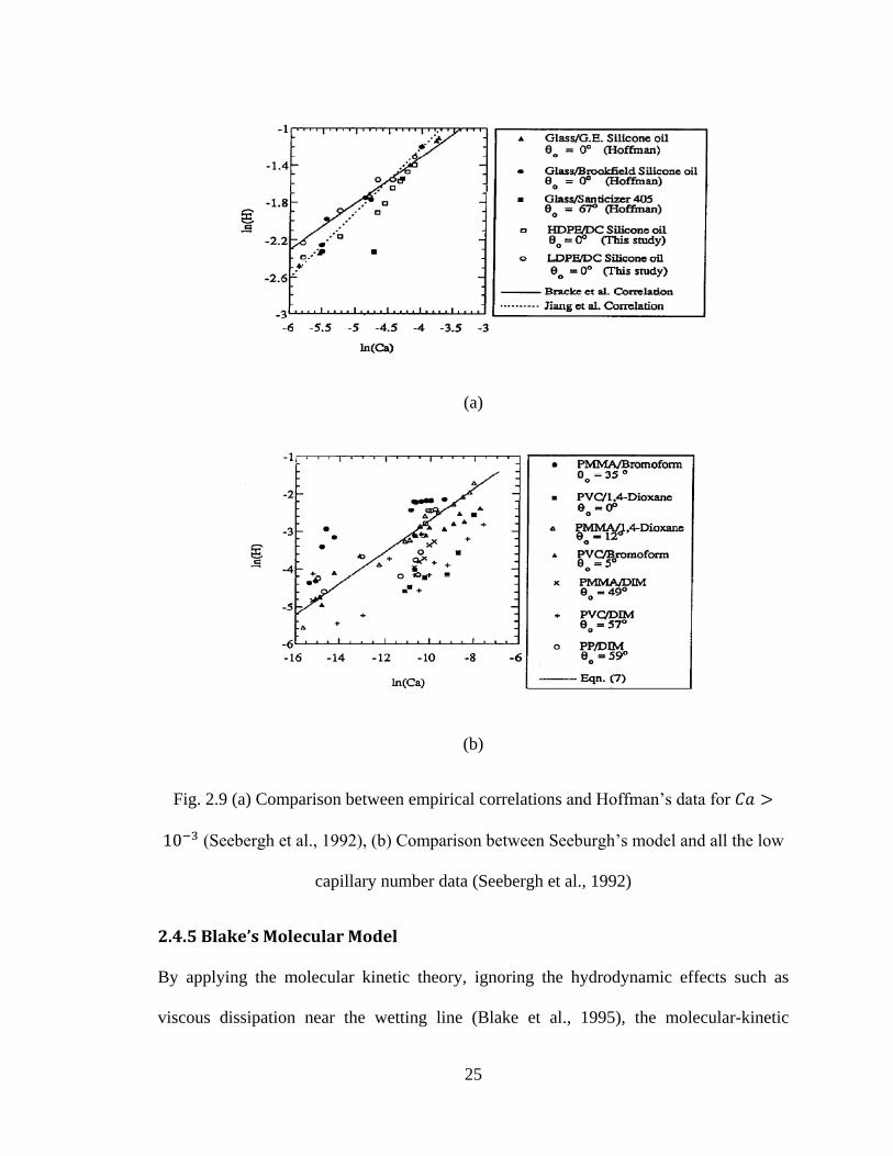
(a)
(b)
Fig. 2.9 (a) Comparison between empirical correlations and Hoffman’s data for 𝐶𝑎 >
10−3 (Seebergh et al., 1992), (b) Comparison between Seeburgh’s model and all the low
capillary number data (Seebergh et al., 1992)
2.4.5 Blake’s Molecular Model
By applying the molecular kinetic theory, ignoring the hydrodynamic effects such as
viscous dissipation near the wetting line (Blake et al., 1995), the molecular-kinetic
26
models take the solid-surface characteristics into account. In this type of model, the
contact line motion is determined by the statistical dynamics of the molecules at the triple
line location (Eral et al., 2013). Two important fitting parameter factors are introduced
here: 𝜅0, the equilibrium frequency of the random molecular displacements occurring at
the triple line location, and 𝜆, the average distance between the adsorption/desorption
sites on the solid surface, see Equ. (2.18 and 2.19). It is assumed that the dynamic
contact angle velocity is depending on the disturbance of the liquid adsorption
equilibrium and the changes in the local surface tension when the wetting line moves
across the solid surface (Eral et al., 2013). Therefore, the driving force for the triple line
motion is expressed as:
𝐹𝑤 = 𝛾𝐿𝑉(𝑐𝑜𝑠 𝜃 −𝑐𝑜𝑠 𝜃𝐷) (2.18)
The resulting from the driving force relationship between contact angle and the wetting
velocity is:
𝑈(𝜃) = 2𝜅0𝜆 sinh[ 𝛾𝐿𝑉(𝑐𝑜𝑠 𝜃 −𝑐𝑜𝑠 𝜃𝐷)𝜆2/2𝑘𝐵𝑇] (2.19)
where 𝑘𝐵 is the Boltzmann constant, and T is the absolute temperature. Eq. (2.19) can
also be expressed as:
𝑐𝑜𝑠 𝜃𝐷 = 𝑐𝑜𝑠 𝜃 −2𝑘𝐵𝑇
𝛾𝐿𝑉𝜆2 𝑠𝑖𝑛ℎ−1(𝑈
2𝜅0𝜆) (2.20)
2.5 Near-reactive (molten metal) case: CAB Technology description
Liquid metal wetting and spreading is essential for many technological processes, e.g.,
spreading of the solder/braze over/between the substrate materials. It is customary to
27
specify that the contact angle must be below 90° for metal bonding (Eustathopoulos et al.,
1999). The triple line movement, defined as a movement of the locus of points between
solid-liquid-gas phases, is the central phenomenon in the manifestation of the kinetics of
a wetting process in liquid metal systems. The mechanical strength and durability of a
solder/braze joint directly rely on the wetting and spreading kinetics process over the
mating surfaces that precede solidification. The wetting (the ability of a liquid to
maintain contact with a solid surface) and spreading (the ability of a liquid to spread on
another liquid or solid) processes in the liquid metal systems mostly involve reactive
interaction across the liquid/solid interface, and the kinetics of the process is not only a
function of viscosity, density, species composition, surface properties, such as roughness,
porosity and electric charges, but also of diffusion, dissolution, convection, deoxidation,
and interfacial reaction (Eustathopoulos et al., 1999; Meier et al., 1999; Saiz et al., 1998;
Contreras et al., 2003; Meier et al., 1998; Rado et al., 2000). The empirical models are
established in most cases by fitting experimental data on triple line movement distance as
a function of time r(t) (Mortensen et al., 1997; Bailey et al., 1951; Li et al., 1992), or
time dependent contact angle θ(t) (Dezellus et al., 2002). Common experimental
methods are known as sessile drop experiments, wetting balance technique
(Eustathopoulos et al., 1999) and hot stage microscopy experiments (Thorsen et al., 1984).
In the manufacturing process, in order to prevent the formation of the oxide layers on the
surface of liquid metals, inert gaseous environment is generally required in the process
setups. For aluminum brazing, the wetting in the inert gaseous (usually nitrogen)
environment is known as the controlled atmosphere brazing process (CAB process).
Figure 2.10 offers an illustration of the CAB facility used in this study.
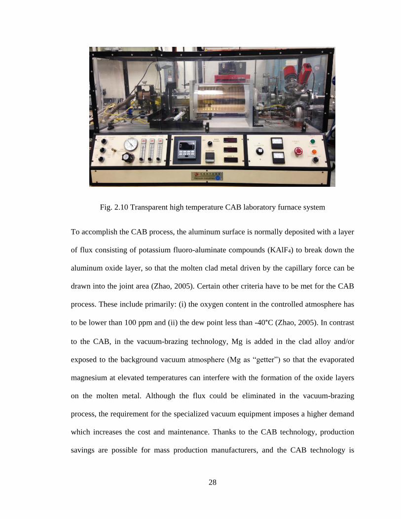
28
Fig. 2.10 Transparent high temperature CAB laboratory furnace system
To accomplish the CAB process, the aluminum surface is normally deposited with a layer
of flux consisting of potassium fluoro-aluminate compounds (KAlF4) to break down the
aluminum oxide layer, so that the molten clad metal driven by the capillary force can be
drawn into the joint area (Zhao, 2005). Certain other criteria have to be met for the CAB
process. These include primarily: (i) the oxygen content in the controlled atmosphere has
to be lower than 100 ppm and (ii) the dew point less than -40°C (Zhao, 2005). In contrast
to the CAB, in the vacuum-brazing technology, Mg is added in the clad alloy and/or
exposed to the background vacuum atmosphere (Mg as “getter”) so that the evaporated
magnesium at elevated temperatures can interfere with the formation of the oxide layers
on the molten metal. Although the flux could be eliminated in the vacuum-brazing
process, the requirement for the specialized vacuum equipment imposes a higher demand
which increases the cost and maintenance. Thanks to the CAB technology, production
savings are possible for mass production manufacturers, and the CAB technology is
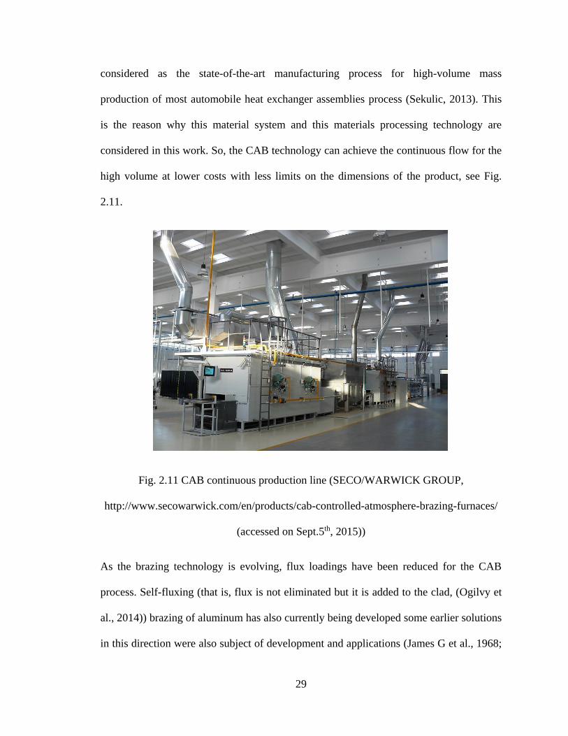
29
considered as the state-of-the-art manufacturing process for high-volume mass
production of most automobile heat exchanger assemblies process (Sekulic, 2013). This
is the reason why this material system and this materials processing technology are
considered in this work. So, the CAB technology can achieve the continuous flow for the
high volume at lower costs with less limits on the dimensions of the product, see Fig.
2.11.
Fig. 2.11 CAB continuous production line (SECO/WARWICK GROUP,
http://www.secowarwick.com/en/products/cab-controlled-atmosphere-brazing-furnaces/
(accessed on Sept.5th, 2015))
As the brazing technology is evolving, flux loadings have been reduced for the CAB
process. Self-fluxing (that is, flux is not eliminated but it is added to the clad, (Ogilvy et
al., 2014)) brazing of aluminum has also currently being developed some earlier solutions
in this direction were also subject of development and applications (James G et al., 1968;
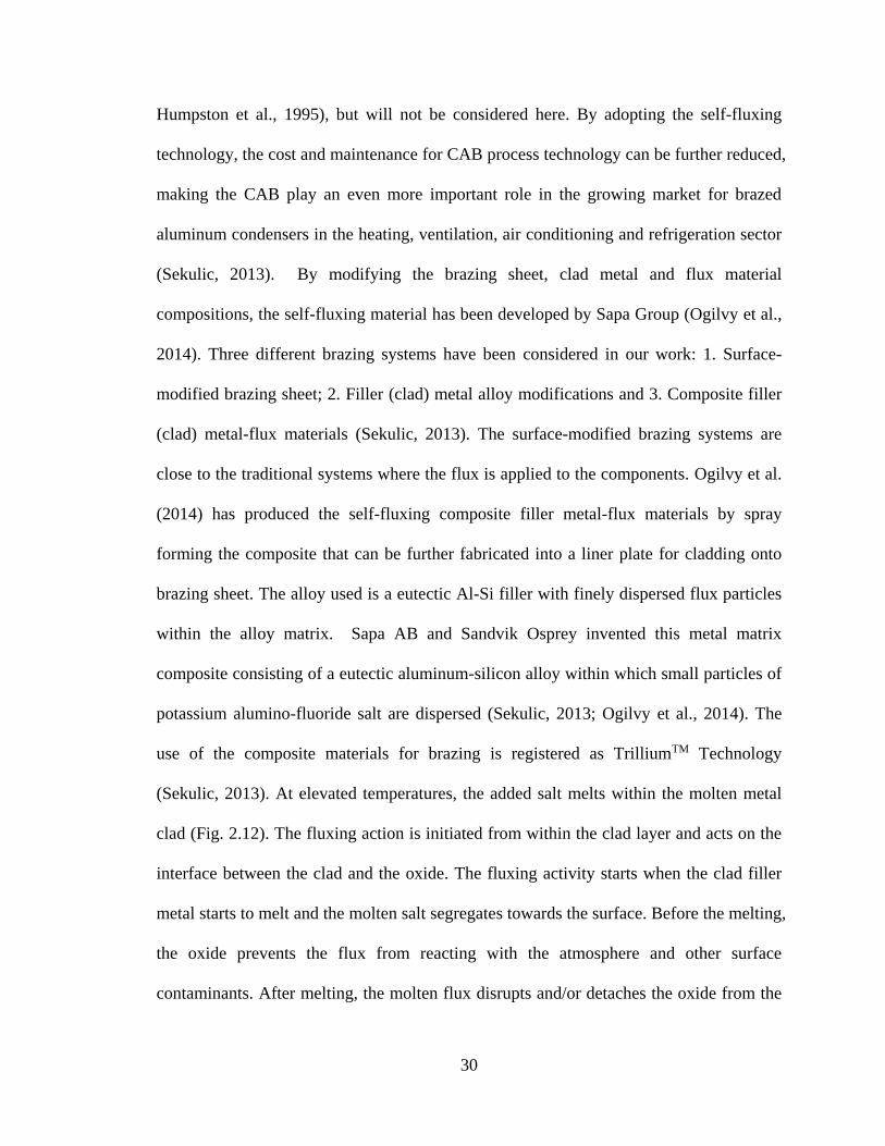
30
Humpston et al., 1995), but will not be considered here. By adopting the self-fluxing
technology, the cost and maintenance for CAB process technology can be further reduced,
making the CAB play an even more important role in the growing market for brazed
aluminum condensers in the heating, ventilation, air conditioning and refrigeration sector
(Sekulic, 2013). By modifying the brazing sheet, clad metal and flux material
compositions, the self-fluxing material has been developed by Sapa Group (Ogilvy et al.,
2014). Three different brazing systems have been considered in our work: 1. Surface-
modified brazing sheet; 2. Filler (clad) metal alloy modifications and 3. Composite filler
(clad) metal-flux materials (Sekulic, 2013). The surface-modified brazing systems are
close to the traditional systems where the flux is applied to the components. Ogilvy et al.
(2014) has produced the self-fluxing composite filler metal-flux materials by spray
forming the composite that can be further fabricated into a liner plate for cladding onto
brazing sheet. The alloy used is a eutectic Al-Si filler with finely dispersed flux particles
within the alloy matrix. Sapa AB and Sandvik Osprey invented this metal matrix
composite consisting of a eutectic aluminum-silicon alloy within which small particles of
potassium alumino-fluoride salt are dispersed (Sekulic, 2013; Ogilvy et al., 2014). The
use of the composite materials for brazing is registered as TrilliumTM Technology
(Sekulic, 2013). At elevated temperatures, the added salt melts within the molten metal
clad (Fig. 2.12). The fluxing action is initiated from within the clad layer and acts on the
interface between the clad and the oxide. The fluxing activity starts when the clad filler
metal starts to melt and the molten salt segregates towards the surface. Before the melting,
the oxide prevents the flux from reacting with the atmosphere and other surface
contaminants. After melting, the molten flux disrupts and/or detaches the oxide from the
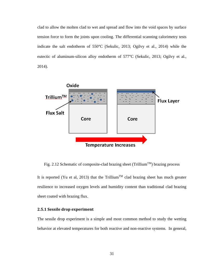
31
clad to allow the molten clad to wet and spread and flow into the void spaces by surface
tension force to form the joints upon cooling. The differential scanning calorimetry tests
indicate the salt endotherm of 550°C (Sekulic, 2013; Ogilvy et al., 2014) while the
eutectic of aluminum-silicon alloy endotherm of 577°C (Sekulic, 2013; Ogilvy et al.,
2014).
Fig. 2.12 Schematic of composite-clad brazing sheet (TrilliumTM) brazing process
It is reported (Yu et al, 2013) that the TrilliumTM clad brazing sheet has much greater
resilience to increased oxygen levels and humidity content than traditional clad brazing
sheet coated with brazing flux.
2.5.1 Sessile drop experiment
The sessile drop experiment is a simple and most common method to study the wetting
behavior at elevated temperatures for both reactive and non-reactive systems. In general,
32
the experiment is designed to permit a drop of liquid to spread over a horizontal solid
substrate until the equilibrium state is reached, see Fig. 2.13.
Fig. 2.13 Schematic of the profiles as the solid cube melts to wet and spread during the
sessile drop experiment
The rate of the liquid front (triple line location) advances over the substrate is the
characteristic of the kinetics of the liquid metal wetting to study. Liquid surface tension
𝛾𝐿𝑉 can also be evaluated from the sessile drop experiments (Keene et al., 1993; Anson et
al., 1999, Fu et al., 2013). To measure the accurate contact angle, smaller sizes of the
drops are recommended, while the surface tension measurement requires larger drops so
that the gravitational force would have impact on the shape of the drop. For the sessile
drop experiment, different forms of the experiment setups could apply, but the common
requirements include the horizontal stage, a furnace chamber to provide either vacuum or
controlled atmosphere condition, heating facility and the measurement facility
(Eustathopoulos, 1999). In order to prevent the oxide layer formation at the elevated
temperature, the test furnace chamber normally is gas tight, so that the chamber can be
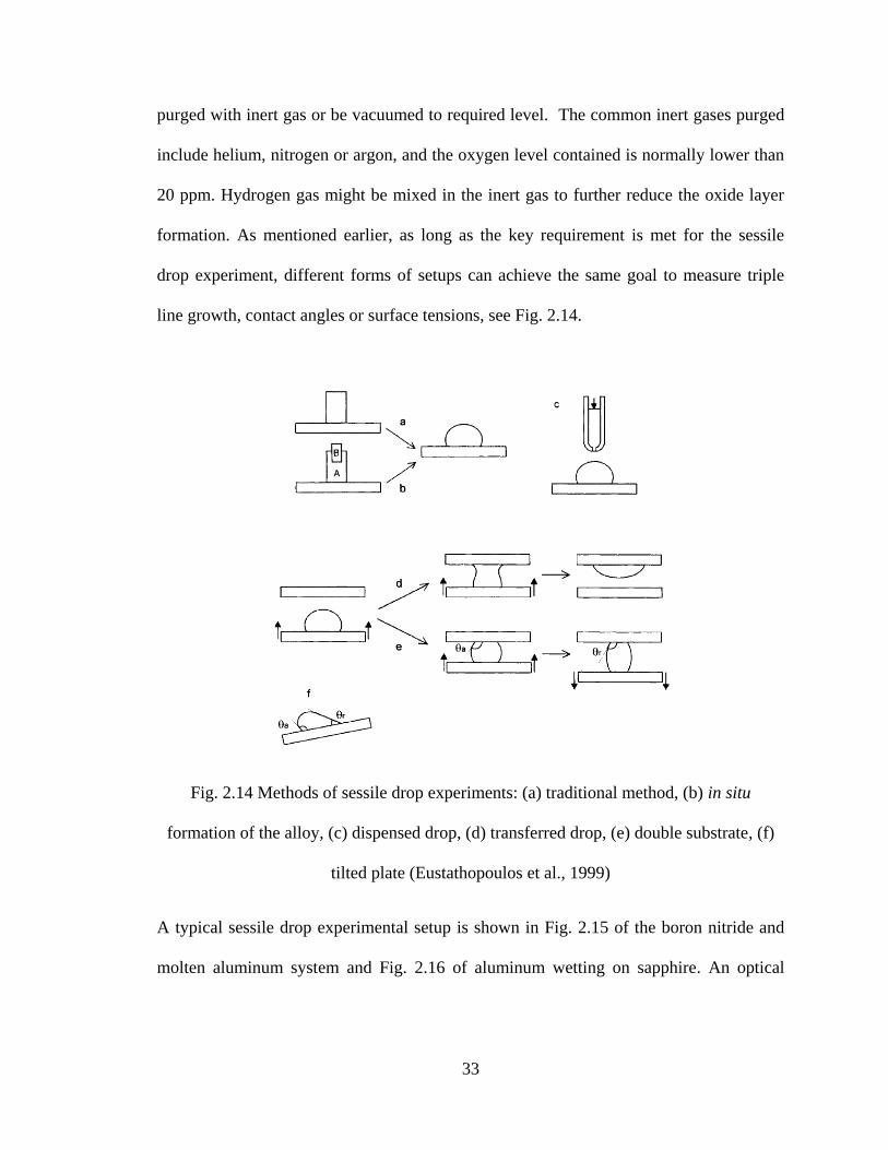
33
purged with inert gas or be vacuumed to required level. The common inert gases purged
include helium, nitrogen or argon, and the oxygen level contained is normally lower than
20 ppm. Hydrogen gas might be mixed in the inert gas to further reduce the oxide layer
formation. As mentioned earlier, as long as the key requirement is met for the sessile
drop experiment, different forms of setups can achieve the same goal to measure triple
line growth, contact angles or surface tensions, see Fig. 2.14.
Fig. 2.14 Methods of sessile drop experiments: (a) traditional method, (b) in situ
formation of the alloy, (c) dispensed drop, (d) transferred drop, (e) double substrate, (f)
tilted plate (Eustathopoulos et al., 1999)
A typical sessile drop experimental setup is shown in Fig. 2.15 of the boron nitride and
molten aluminum system and Fig. 2.16 of aluminum wetting on sapphire. An optical
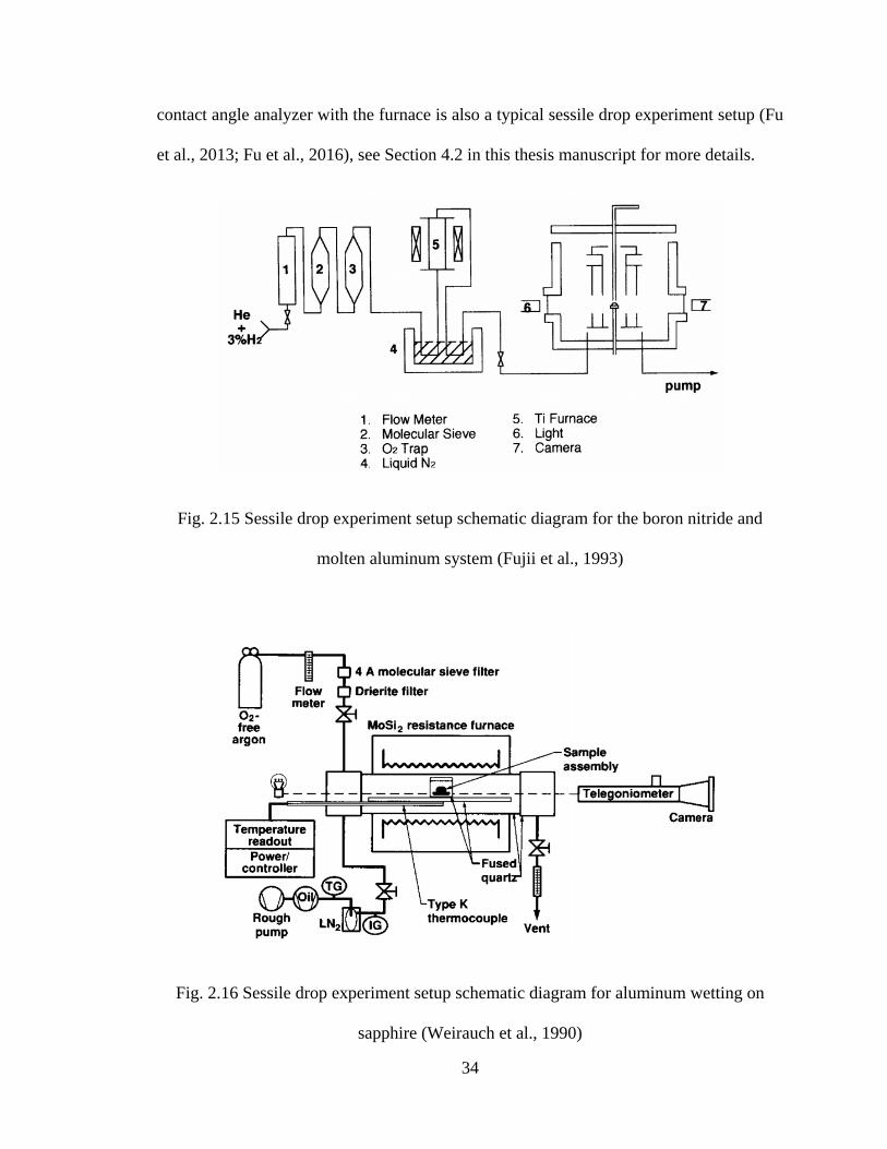
34
contact angle analyzer with the furnace is also a typical sessile drop experiment setup (Fu
et al., 2013; Fu et al., 2016), see Section 4.2 in this thesis manuscript for more details.
Fig. 2.15 Sessile drop experiment setup schematic diagram for the boron nitride and
molten aluminum system (Fujii et al., 1993)
Fig. 2.16 Sessile drop experiment setup schematic diagram for aluminum wetting on
sapphire (Weirauch et al., 1990)
35
The spherical drop volume 𝑣 can be calculated based on the following equation
(Eustathopoulos et al., 1999) :
𝑣 =𝜋𝑅3
3
(2−3𝑐𝑜𝑠𝜃+𝑐𝑜𝑠3𝜃)
𝑠𝑖𝑛3𝜃 (2.21)
where R is the radius of the drop, 𝜃 is the contact angle.
Since R has to be measure after the experiment is completed, alternatively, one can also
use the Bashforth and Adams tables (1883) to calculate the volume as:
𝑣 = 𝜋𝑅2 (2𝑏
𝛽−
2𝑏2𝑠𝑖𝑛𝜃
𝑥90𝛽+ 𝐻);
𝛽 =𝑏2𝜌𝑔
𝛾𝐿𝑉 (2.21)
where H is the drop height, 𝜌 is the liquid density, 𝑔 is the gravitational force, 𝛾𝐿𝑉 is the
surface tension and 𝑥90 is the constant from Bashforth and Adams tables.
The wetting kinetics can be presented from the sessile drop experiments by measuring the
triple line locations and time relationships (Fu et al., 2013; Fu et al., 2016). Further
discussion will be made in later chapters.
2.5.2 Wetting balance experiment
The wetting balance experiment is referring to the pulling or inserting an object into the
liquid surface to measure the surface tension (Eustathopoulos et al., 1999), corresponding
the Wilhelmy plate configuration in the non-reactive experiments. As was described by
Chappius et al. (1982), the wetting balance method consists of continuously monitoring
the force acting on a solid, cylinder or blade, moving into and out of a liquid bath during
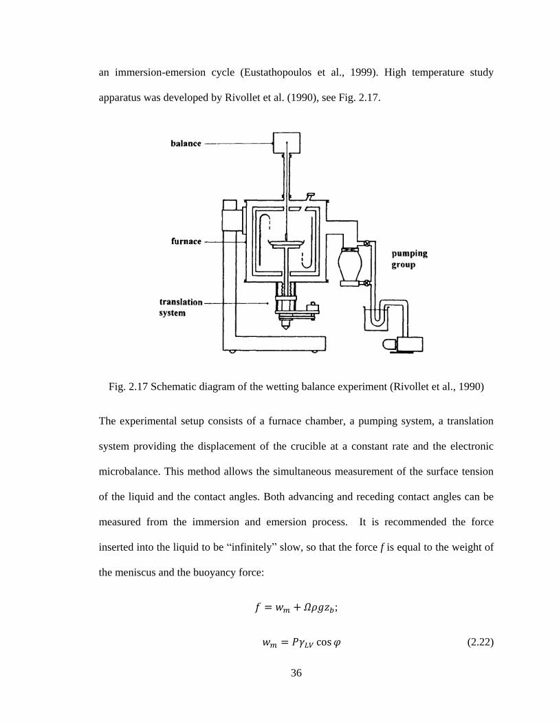
36
an immersion-emersion cycle (Eustathopoulos et al., 1999). High temperature study
apparatus was developed by Rivollet et al. (1990), see Fig. 2.17.
Fig. 2.17 Schematic diagram of the wetting balance experiment (Rivollet et al., 1990)
The experimental setup consists of a furnace chamber, a pumping system, a translation
system providing the displacement of the crucible at a constant rate and the electronic
microbalance. This method allows the simultaneous measurement of the surface tension
of the liquid and the contact angles. Both advancing and receding contact angles can be
measured from the immersion and emersion process. It is recommended the force
inserted into the liquid to be “infinitely” slow, so that the force f is equal to the weight of
the meniscus and the buoyancy force:
𝑓 = 𝑤𝑚 + 𝛺𝜌𝑔𝑧𝑏;
𝑤𝑚 = 𝑃𝛾𝐿𝑉 cos 𝜑 (2.22)
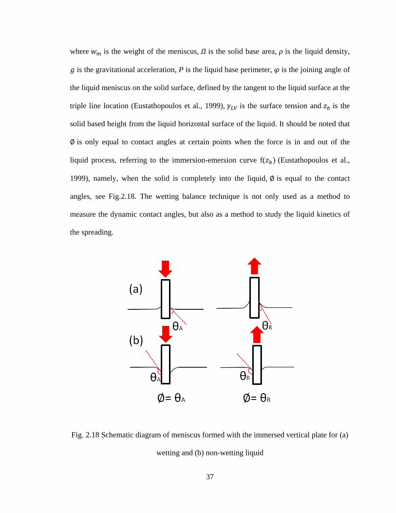
37
where 𝑤𝑚 is the weight of the meniscus, 𝛺 is the solid base area, 𝜌 is the liquid density,
𝑔 is the gravitational acceleration, P is the liquid base perimeter, 𝜑 is the joining angle of
the liquid meniscus on the solid surface, defined by the tangent to the liquid surface at the
triple line location (Eustathopoulos et al., 1999), 𝛾𝐿𝑉 is the surface tension and 𝑧𝑏 is the
solid based height from the liquid horizontal surface of the liquid. It should be noted that
∅ is only equal to contact angles at certain points when the force is in and out of the
liquid process, referring to the immersion-emersion curve f(𝑧𝑏) (Eustathopoulos et al.,
1999), namely, when the solid is completely into the liquid, ∅ is equal to the contact
angles, see Fig.2.18. The wetting balance technique is not only used as a method to
measure the dynamic contact angles, but also as a method to study the liquid kinetics of
the spreading.
Fig. 2.18 Schematic diagram of meniscus formed with the immersed vertical plate for (a)
wetting and (b) non-wetting liquid
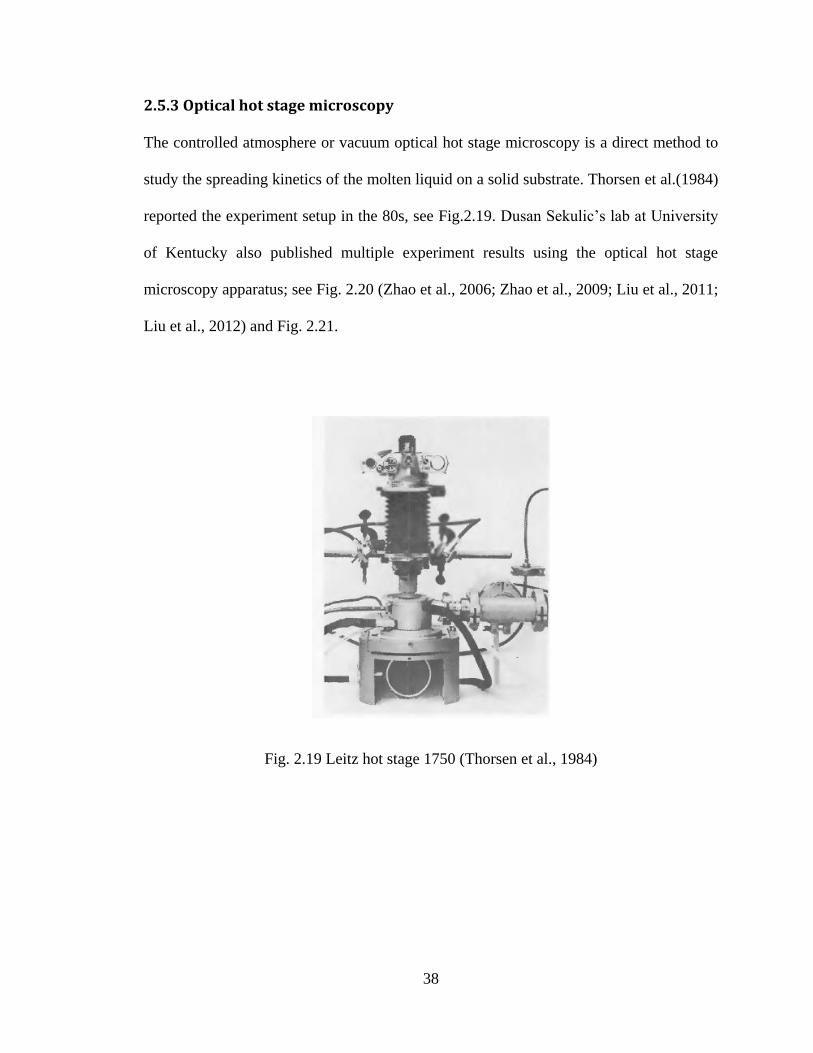
38
2.5.3 Optical hot stage microscopy
The controlled atmosphere or vacuum optical hot stage microscopy is a direct method to
study the spreading kinetics of the molten liquid on a solid substrate. Thorsen et al.(1984)
reported the experiment setup in the 80s, see Fig.2.19. Dusan Sekulic’s lab at University
of Kentucky also published multiple experiment results using the optical hot stage
microscopy apparatus; see Fig. 2.20 (Zhao et al., 2006; Zhao et al., 2009; Liu et al., 2011;
Liu et al., 2012) and Fig. 2.21.
Fig. 2.19 Leitz hot stage 1750 (Thorsen et al., 1984)
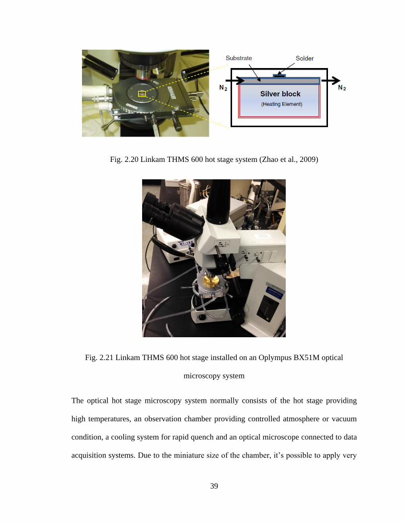
39
Fig. 2.20 Linkam THMS 600 hot stage system (Zhao et al., 2009)
Fig. 2.21 Linkam THMS 600 hot stage installed on an Oplympus BX51M optical
microscopy system
The optical hot stage microscopy system normally consists of the hot stage providing
high temperatures, an observation chamber providing controlled atmosphere or vacuum
condition, a cooling system for rapid quench and an optical microscope connected to data
acquisition systems. Due to the miniature size of the chamber, it’s possible to apply very
40
fast heating rate and cooling at fast recording speed. It has been reported the heating rate
can reach to 100°C/min and the cooling ramp of 80°C/min (Zhao et al., 2009). Inert gas
can be purged into the test chamber or vacuum condition. Due to its small volume,
multiple gas volume replacement can take place in a certain period of time. Since the real
time video can be captured by the video camera mounted on the microscope, wetting
kinetics can be investigated frame by frame with professional image analysis software.
Such experiment setup is used to study the molten metal fast spreading process in a short
period of time, and offers the direct understanding of kinetics features for different
molten metal systems. The surface roughness impact on wetting was also investigated
(Wen et al., 2012). The contact angles cannot be measured in this method (the field of
vision is from the top). It is also not recommended to study a non-wetting/spreading
molten metal on a solid substrate.
2.6 Wetting kinetics theories and models at elevated temperatures
The near non-reactive wetting of molten metals and oxides on molybdenum was studied
by Saiz et al. (2007) as an initial step to analyze more complex reactive systems. Without
interfacial reactions, the spreading is dominated by dissipation at the triple line location
caused by the much stronger atomic interactions compared to organic liquids at low
temperatures. As investigated by Voytovych et al. (2007), at high temperatures, the
reactive wetting is controlled by compound formation at the interface. Lee et al. (2003)
also pointed out that wetting is impacted by both the interfacial reactions and the
compound formation at the interface. The spreading can be categorized into three regimes:
(i) impact, (ii) inertial and (iii) capillary regime. In the impact regime, the drop hits the
substrate (if impacting the substrate at the onset of spreading) and the subsequent flow is
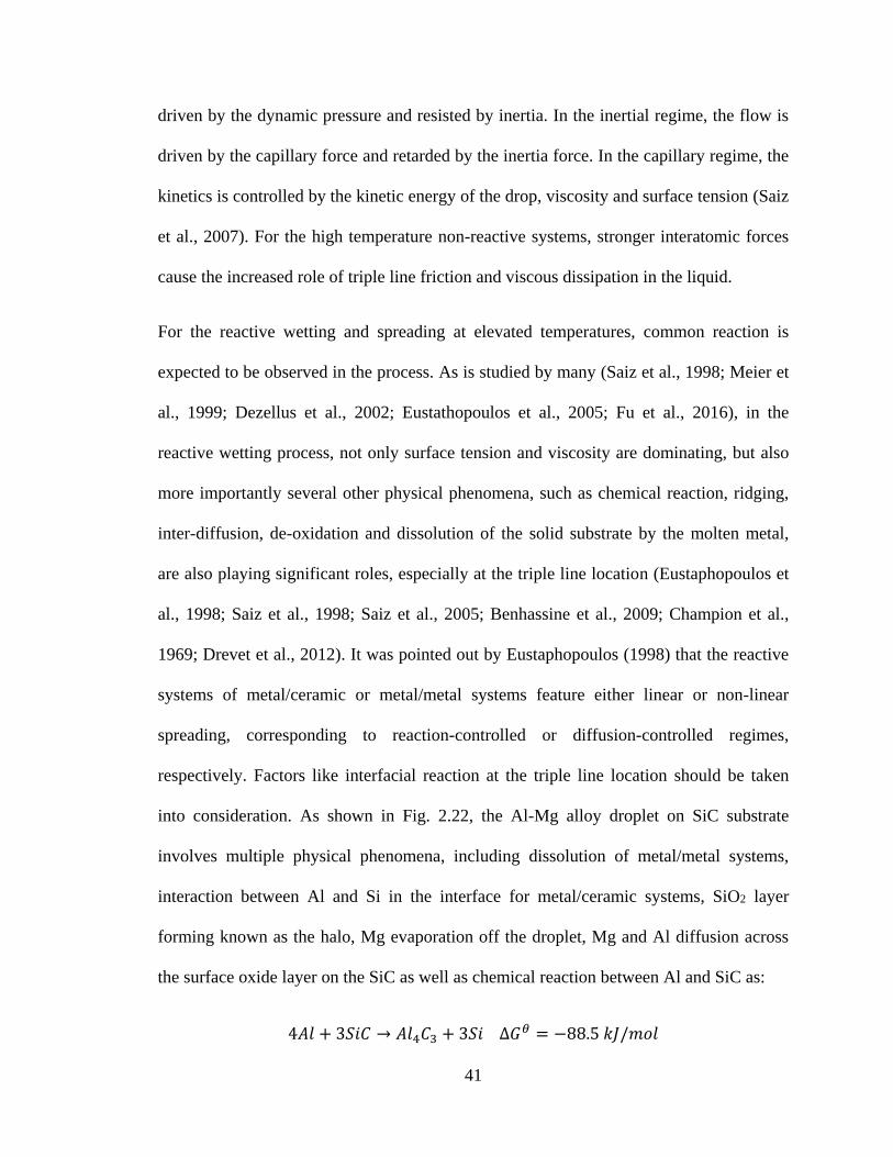
41
driven by the dynamic pressure and resisted by inertia. In the inertial regime, the flow is
driven by the capillary force and retarded by the inertia force. In the capillary regime, the
kinetics is controlled by the kinetic energy of the drop, viscosity and surface tension (Saiz
et al., 2007). For the high temperature non-reactive systems, stronger interatomic forces
cause the increased role of triple line friction and viscous dissipation in the liquid.
For the reactive wetting and spreading at elevated temperatures, common reaction is
expected to be observed in the process. As is studied by many (Saiz et al., 1998; Meier et
al., 1999; Dezellus et al., 2002; Eustathopoulos et al., 2005; Fu et al., 2016), in the
reactive wetting process, not only surface tension and viscosity are dominating, but also
more importantly several other physical phenomena, such as chemical reaction, ridging,
inter-diffusion, de-oxidation and dissolution of the solid substrate by the molten metal,
are also playing significant roles, especially at the triple line location (Eustaphopoulos et
al., 1998; Saiz et al., 1998; Saiz et al., 2005; Benhassine et al., 2009; Champion et al.,
1969; Drevet et al., 2012). It was pointed out by Eustaphopoulos (1998) that the reactive
systems of metal/ceramic or metal/metal systems feature either linear or non-linear
spreading, corresponding to reaction-controlled or diffusion-controlled regimes,
respectively. Factors like interfacial reaction at the triple line location should be taken
into consideration. As shown in Fig. 2.22, the Al-Mg alloy droplet on SiC substrate
involves multiple physical phenomena, including dissolution of metal/metal systems,
interaction between Al and Si in the interface for metal/ceramic systems, SiO2 layer
forming known as the halo, Mg evaporation off the droplet, Mg and Al diffusion across
the surface oxide layer on the SiC as well as chemical reaction between Al and SiC as:
4𝐴𝑙 + 3𝑆𝑖𝐶 → 𝐴𝑙4𝐶3 + 3𝑆𝑖 ∆𝐺𝜃 = −88.5 𝑘𝐽/𝑚𝑜𝑙
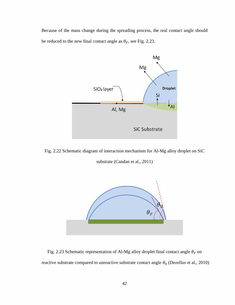
42
Because of the mass change during the spreading process, the real contact angle should
be reduced to the new final contact angle as 𝜃𝐹, see Fig. 2.23.
Fig. 2.22 Schematic diagram of interaction mechanism for Al-Mg alloy droplet on SiC
substrate (Candan et al., 2011)
Fig. 2.23 Schematic representation of Al-Mg alloy droplet final contact angle 𝜃𝐹 on
reactive substrate compared to unreactive substrate contact angle 𝜃0 (Dezellus et al., 2010)
43
As is pointed out by Dezellus et al. (2010), at elevated temperatures for the reactive
wetting, spreading kinetics is not limited by viscous dissipation but by the rate of
interfacial reaction at the triple line location. The interfacial reaction rate is controlled by
the slower of two successive phenomena that happen in the reaction process: diffusive
transport of reacting species to or from the triple line location and local reaction kinetics
at the triple line location (Dezellus et al., 2010). The new compound formed at the
interfacial layer due to reaction can either improve wetting or reduce wetting, depending
on wettability by molten metal of new compound compared to the wettability of the
initial solid substrate.
2.6.1 Diffusion-controlled wetting of metal/ceramic systems model
In a sessile drop experiment configuration on metal/ceramic systems, the metal drop
forms on a solid substrate, and when starts deforming rapidly controlled by viscous force,
the initial contact angle 𝜃𝐷 equals the same contact angle of the liquid on the original
unreacted substrate. Then as the droplet spreads with the reaction proceeding between
metal and the substrate, the final contact angle 𝜃𝐹 will form after a longer period of time.
During the spreading process, a reactive penetration of species normally occurs (Saiz et
al., 1998). As was pointed out by Saiz et al. (2005), the formed ridge at the triple line
location, formed due to local diffusion or solution precipitation, can hinder the spreading
of the triple line. It is known that the final contact angle is not related to capillary force
dominated spreading, but rather to the reaction product layer formed and droplet volume.
Namely, the reaction at the triple line location (Dezellus et al., 2002) a key process. Two
spreading regimes can be observed during the process, known as the first linear regime
and the second diffusion dominated non-linear regime. For the wetting of metal/ceramic
44
systems without dissolution, Mortensen et al. (1997) modeled the diffusion-controlled
wetting. According to the model, the isothermal spreading kinetics is proportional to the
dynamic contact angle:
𝑑𝑅
𝑑𝑡=
2𝐷𝐹(𝑡)
𝑒𝑛𝑣(𝐶0 − 𝐶𝑒)𝜃𝐷 (2.23)
where D is the diffusion coefficient in the liquid, 𝑛𝑣 is the number of moles of reactive
solute per unit volume of the reaction product, 𝑒 is the reaction product thickness at the
triple line location, 𝐹(𝑡) is a function of time which can be considered as a constant of
0.04 for most sessile drop experiments, 𝐶0 is the nominal drop reactive solute
concentration, 𝐶𝑒 is the concentration of reactive solute in equilibrium with the reactive
product, R is the perimeter of the droplet and 𝜃𝐷 is the dynamic contact angle (Mortensen
et al., 1997).
The isothermal spreading by metal/ceramic systems limited by solute diffusion at the
triple line location showed good agreement with experimental results for AgCuSn-Ti/Cu
systems (Dezellus et al., 2010). For Cu-Cr/Cu systems, certain modification to the contact
angle is needed for the validity of Eq. (2.23) (Dezellus et al., 2010).
2.6.2 Dissolutive wetting model
Similar to the metal/ceramic systems, wetting for the metal/metal systems is controlled
by compound formation at the interface (Voytovych et al., 2007). Four stages of wetting
in metal/metal systems can be observed (Yin et al., 2009). The first stage is the initial
regime where the liquid spreads with no obvious reaction dominated by the capillary
force; the second stage is a highly reactive regime where reaction and the morphological
and chemical changes can take place at the liquid and solid interface; the third stage is a
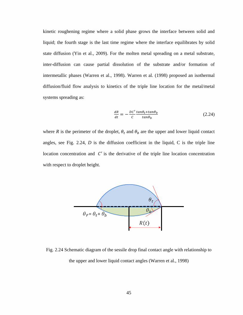
45
kinetic roughening regime where a solid phase grows the interface between solid and
liquid; the fourth stage is the last time regime where the interface equilibrates by solid
state diffusion (Yin et al., 2009). For the molten metal spreading on a metal substrate,
inter-diffusion can cause partial dissolution of the substrate and/or formation of
intermetallic phases (Warren et al., 1998). Warren et al. (1998) proposed an isothermal
diffusion/fluid flow analysis to kinetics of the triple line location for the metal/metal
systems spreading as:
𝑑𝑅
𝑑𝑡= −
𝐷𝐶′
𝐶
𝑡𝑎𝑛𝜃𝑡+𝑡𝑎𝑛𝜃𝑏
𝑡𝑎𝑛𝜃𝑏 (2.24)
where R is the perimeter of the droplet, 𝜃𝑡 and 𝜃𝑏 are the upper and lower liquid contact
angles, see Fig. 2.24, D is the diffusion coefficient in the liquid, C is the triple line
location concentration and 𝐶′ is the derivative of the triple line location concentration
with respect to droplet height.
Fig. 2.24 Schematic diagram of the sessile drop final contact angle with relationship to
the upper and lower liquid contact angles (Warren et al., 1998)
46
The dissolution spreading process can also be relevant in some metal/ceramic systems
such as AuNi/ZrB2 (Voytovych et al., 2007) and Ni/C systems (Eustaphopoulos, 1999).
A quasi-linear reactive stage empirical correlation is also modeled by Dezellus et al.
(2002). This correlation is valid for the triple line location kinetics that is controlled by
the process of atom transfer occurring at the substrate/liquid alloy interface. The
correlation is as follows:
𝑈
𝐹(𝜃𝐷)= 𝑘 (
3𝑣
𝜋) (𝑐𝑜𝑠𝜃 − 𝑐𝑜𝑠𝜃𝐷);
𝐹(𝜃𝐷) =𝑐𝑜𝑠𝜃(2−3𝑐𝑜𝑠𝜃𝐷+𝑐𝑜𝑠3𝜃𝐷)−𝑠𝑖𝑛4𝜃𝐷
𝑠𝑖𝑛𝜃𝐷(2−3𝑐𝑜𝑠𝜃𝐷+𝑐𝑜𝑠3𝜃𝐷)4/3 (2.25)
where 𝑈 is the triple line movement velocity, 𝑣 is the droplet volume, 𝑘 is the constant
proportional to the kinetics constant of the dissolution process and to the driving force of
the dissolution process, 𝜃𝐷 is the dynamic contact angle, 𝜃 is the contact angle. This type
of empirical model was well verified by Calderon et al. (2010) using experimental data
for Al-Si alloys on carbon substrates. The spreading kinetics increases with temperature
and Si content in the alloy, and it is sensitive to the carbon substrate structure (Calderon
et al., 2010). However, this model is not valid for the later stage of the spreading kinetics
which is limited by the diffusion of reactive species in the reactive layer.
This dissolution spreading model has a good agreement for the Sn/Bi system (Calderon et
al., 2010), however, more work and study are needed to have a systematic understanding
of this type of reactive wetting in the future.
47
CHAPTER 3: BENCHMARK STUDY OF THE KINETICS ON A
CAPILLARY FLOW OF NON-REACTIVE LIQUID SYSTEMS
In order to establish the reproducibility of the methods used for the experimental data
collection of Al-Si (Trillium) systems, a series experiments with non-reactive systems
(water and silicon oil on a glass) has been performed. This data were also used to verify
the validity of numerical phase field modeling conducted in the collaborative project.
3.1 Overview
In this chapter, the non-reactive wetting experimental procedure is developed for optical
evaluation of the contact angle in order to generate empirical data sets needed for
theoretical modeling as a benchmark reference involving the reactive wetting evaluation
at elevated temperatures. Two types of liquid systems, namely water and silicone oil, at
ambient temperature are investigated by developing the wedge-tee configuration
spreading. The wedge tee pre-cleaned glasses forming a Wilhelmy-type plate
configuration (a single substrate in contact with the pool of liquid). Both equilibrium
states of the triple line location and the triple line kinetics are studied for verification of
the empirical correlation form derived by various sources, corresponding to Washburn’s
Law (Washburn, 1921) type of power law. The surface tension driven spreading, retarded
by viscosity, at the ambient temperature is considered to be wetting without chemical
reactions. The experimental data and procedures are validated by comparing to the
theoretical triple line spreading height (upon reaching the equilibrium state), as well as
empirical spreading kinetics correlations. This chapter provides a benchmark foundation
48
upon which later chapters involving molten metal reactive spreading kinetics can be
based.
This chapter consists of two parts, (i) the static study of the triple line equilibrium spread,
and (ii) the kinetics study of triple line spreading. The static contact angle of both liquid
systems was proved to obey the theoretical prediction (Seebergh et al., 1992) of the
equilibrium triple line location. The Neumann (1972) theoretical prediction based on
Young’s equation confirms the agreement with data excellently. In the second part of this
chapter, the kinetics of the triple line prediction are verified by different empirical
correlations using the capillary number and dynamic contact angle. The dynamic contact
angle and capillary number of silicone oil system agree with the existing correlation
models, however, the water on glass system showed the deviations to a certain degree
from those known models. A new correlation model was established for the water on
glass system. The liquids wetting on the vertical slides also showed the Washburn flow
pattern in the initial capillary-viscous stage. Hence the wetting was initially driven by
surface tension and retarded by viscosity. The subsequent stage showed a clearly 5th
power law relationship, thus surface tension and viscosity showed a less dramatic impact
on the wetting process.
3.2 Experimental setup and procedure
3.2.1 Material preparation
In order to study the spreading process of non-reactive liquid, the Wilhelmy plate
configuration is adopted in this investigation. Two types of liquids are chosen for the
study of the kinetics of non-reactive liquid systems: deionized water (DI water) and
silicone oil. The properties of the liquids can be found in Table 3.1.
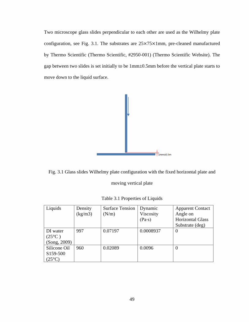
49
Two microscope glass slides perpendicular to each other are used as the Wilhelmy plate
configuration, see Fig. 3.1. The substrates are 25×75×1mm, pre-cleaned manufactured
by Thermo Scientific (Thermo Scientific, #2950-001) (Thermo Scientific Website). The
gap between two slides is set initially to be 1mm±0.5mm before the vertical plate starts to
move down to the liquid surface.
Fig. 3.1 Glass slides Wilhelmy plate configuration with the fixed horizontal plate and
moving vertical plate
Table 3.1 Properties of Liquids
Liquids Density
(kg/m3)
Surface Tension
(N/m)
Dynamic
Viscosity
(Pa∙s)
Apparent Contact
Angle on
Horizontal Glass
Substrate (deg)
DI water
(25°C )
(Song, 2009)
997 0.07197 0.0008937 0
Silicone Oil
S159-500
(25°C)
960 0.02089 0.0096 0
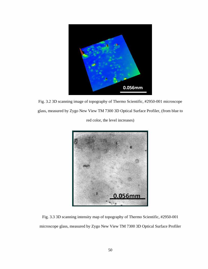
50
Fig. 3.2 3D scanning image of topography of Thermo Scientific, #2950-001 microscope
glass, measured by Zygo New View TM 7300 3D Optical Surface Profiler, (from blue to
red color, the level increases)
Fig. 3.3 3D scanning intensity map of topography of Thermo Scientific, #2950-001
microscope glass, measured by Zygo New View TM 7300 3D Optical Surface Profiler
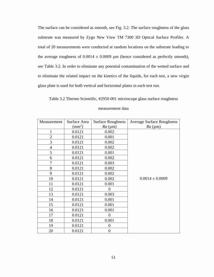
51
The surface can be considered as smooth, see Fig. 3.2. The surface roughness of the glass
substrate was measured by Zygo New View TM 7300 3D Optical Surface Profiler. A
total of 20 measurements were conducted at random locations on the substrate leading to
the average roughness of 0.0014 ± 0.0009 µm (hence considered as perfectly smooth),
see Table 3.2. In order to eliminate any potential contamination of the wetted surface and
to eliminate the related impact on the kinetics of the liquids, for each test, a new virgin
glass plate is used for both vertical and horizontal plates in each test run.
Table 3.2 Thermo Scientific, #2950-001 microscope glass surface roughness
measurement data
Measurement
Surface Area
(mm2)
Surface Roughness
Ra (µm)
Average Surface Roughness
Ra (µm)
1 0.0121 0.002
2 0.0121 0.001
3 0.0121 0.002
4 0.0121 0.002
5 0.0121 0.001
6 0.0121 0.002
7 0.0121 0.003
8 0.0121 0.002
9 0.0121 0.002
10 0.0121 0.002 0.0014 ± 0.0009
11 0.0121 0.001
12 0.0121 0
13 0.0121 0.003
14 0.0121 0.001
15 0.0121 0.001
16 0.0121 0.001
17 0.0121 0
18 0.0121 0.001
19 0.0121 0
20 0.0121 0
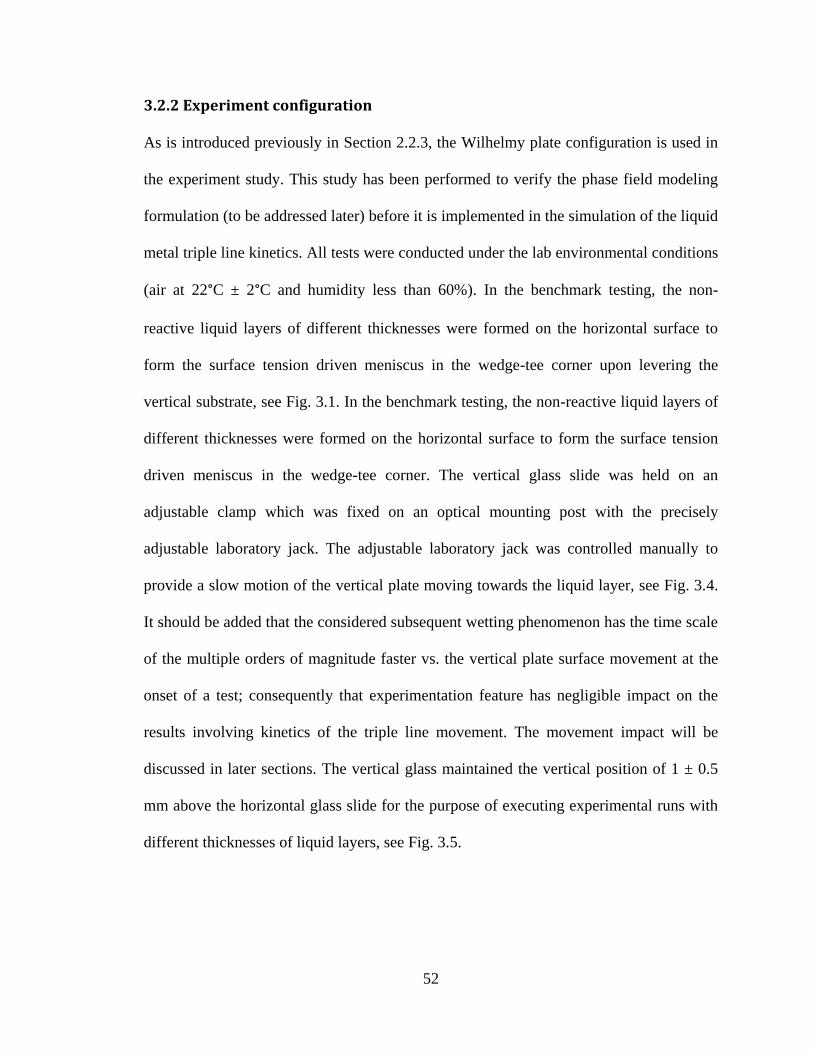
52
3.2.2 Experiment configuration
As is introduced previously in Section 2.2.3, the Wilhelmy plate configuration is used in
the experiment study. This study has been performed to verify the phase field modeling
formulation (to be addressed later) before it is implemented in the simulation of the liquid
metal triple line kinetics. All tests were conducted under the lab environmental conditions
(air at 22°C ± 2°C and humidity less than 60%). In the benchmark testing, the non-
reactive liquid layers of different thicknesses were formed on the horizontal surface to
form the surface tension driven meniscus in the wedge-tee corner upon levering the
vertical substrate, see Fig. 3.1. In the benchmark testing, the non-reactive liquid layers of
different thicknesses were formed on the horizontal surface to form the surface tension
driven meniscus in the wedge-tee corner. The vertical glass slide was held on an
adjustable clamp which was fixed on an optical mounting post with the precisely
adjustable laboratory jack. The adjustable laboratory jack was controlled manually to
provide a slow motion of the vertical plate moving towards the liquid layer, see Fig. 3.4.
It should be added that the considered subsequent wetting phenomenon has the time scale
of the multiple orders of magnitude faster vs. the vertical plate surface movement at the
onset of a test; consequently that experimentation feature has negligible impact on the
results involving kinetics of the triple line movement. The movement impact will be
discussed in later sections. The vertical glass maintained the vertical position of 1 ± 0.5
mm above the horizontal glass slide for the purpose of executing experimental runs with
different thicknesses of liquid layers, see Fig. 3.5.
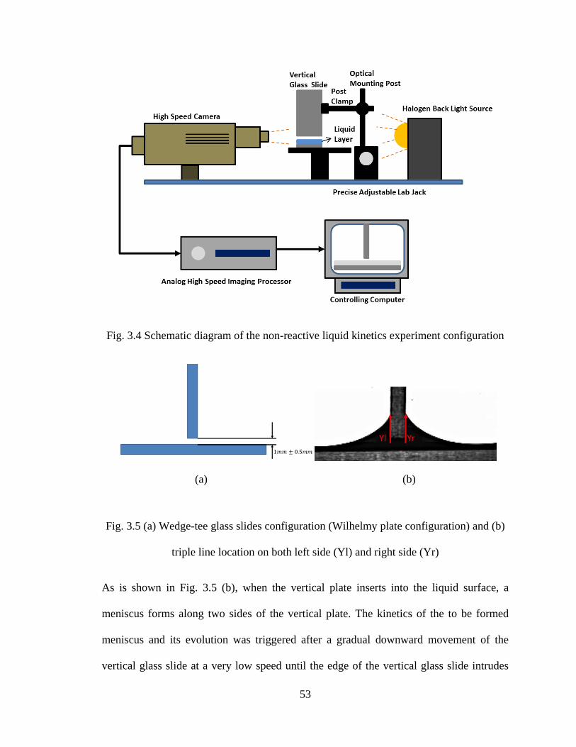
53
Fig. 3.4 Schematic diagram of the non-reactive liquid kinetics experiment configuration
(a) (b)
Fig. 3.5 (a) Wedge-tee glass slides configuration (Wilhelmy plate configuration) and (b)
triple line location on both left side (Yl) and right side (Yr)
As is shown in Fig. 3.5 (b), when the vertical plate inserts into the liquid surface, a
meniscus forms along two sides of the vertical plate. The kinetics of the to be formed
meniscus and its evolution was triggered after a gradual downward movement of the
vertical glass slide at a very low speed until the edge of the vertical glass slide intrudes
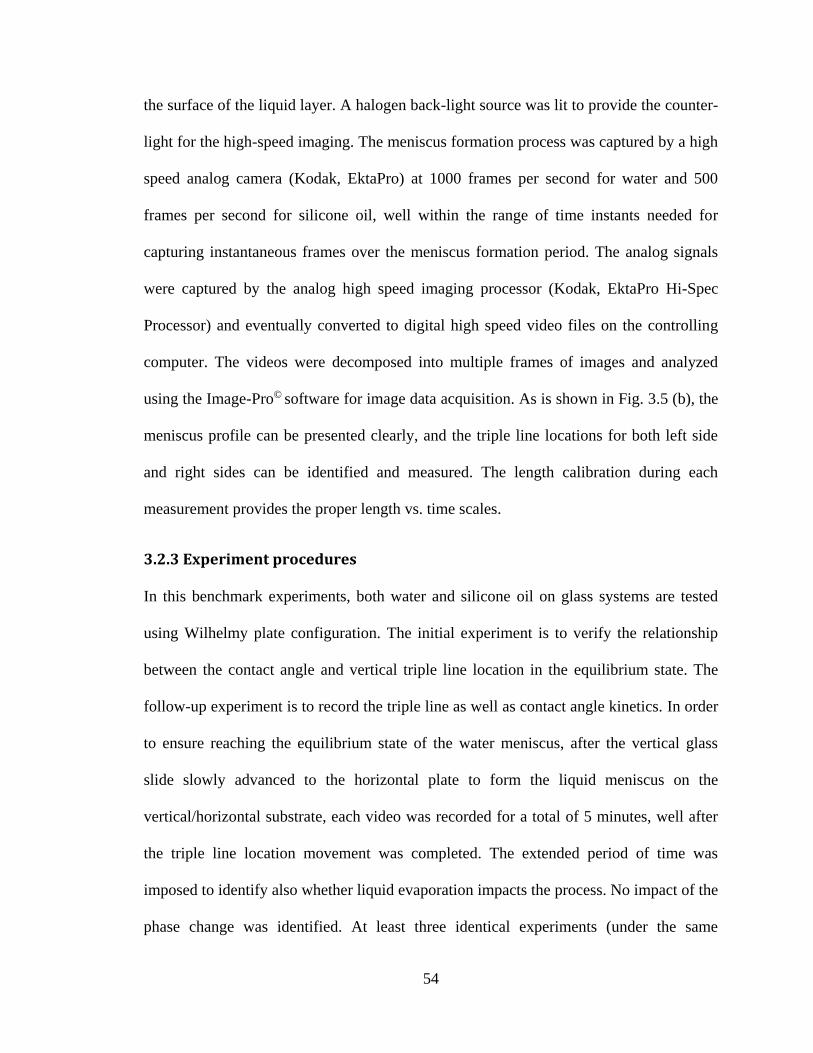
54
the surface of the liquid layer. A halogen back-light source was lit to provide the counter-
light for the high-speed imaging. The meniscus formation process was captured by a high
speed analog camera (Kodak, EktaPro) at 1000 frames per second for water and 500
frames per second for silicone oil, well within the range of time instants needed for
capturing instantaneous frames over the meniscus formation period. The analog signals
were captured by the analog high speed imaging processor (Kodak, EktaPro Hi-Spec
Processor) and eventually converted to digital high speed video files on the controlling
computer. The videos were decomposed into multiple frames of images and analyzed
using the Image-Pro© software for image data acquisition. As is shown in Fig. 3.5 (b), the
meniscus profile can be presented clearly, and the triple line locations for both left side
and right sides can be identified and measured. The length calibration during each
measurement provides the proper length vs. time scales.
3.2.3 Experiment procedures
In this benchmark experiments, both water and silicone oil on glass systems are tested
using Wilhelmy plate configuration. The initial experiment is to verify the relationship
between the contact angle and vertical triple line location in the equilibrium state. The
follow-up experiment is to record the triple line as well as contact angle kinetics. In order
to ensure reaching the equilibrium state of the water meniscus, after the vertical glass
slide slowly advanced to the horizontal plate to form the liquid meniscus on the
vertical/horizontal substrate, each video was recorded for a total of 5 minutes, well after
the triple line location movement was completed. The extended period of time was
imposed to identify also whether liquid evaporation impacts the process. No impact of the
phase change was identified. At least three identical experiments (under the same
55
conditions) were executed for both water and silicone oil systems. Each test was
performed with a new set of pre-cleaned glass substrates. It was found that the already
used glass features surface conditions that may impact the kinetics of the process
regardless of an implemented cleaning treatment in the previous preliminary tests. The
liquid meniscuses of both water and silicone oil were formed well within 2 seconds. As
the videos of the kinetics of both water and silicone oil were recorded by the high speed
camera, images of different frames from the video can be exported to Image-Pro© to
measure the instantaneous dynamic contact angle and the triple line location, see Fig.3.6.
In the case of the water system, the whole kinetics process lasts for the order of
magnitude of 103 ms, whereas the process lasts a bit longer (the same order of magnitude,
2x 10³ ms) in the case of the silicone oil system. For each experiment measurement, a
new calibration of the meareument is required in Image-Pro© before a new measurement.
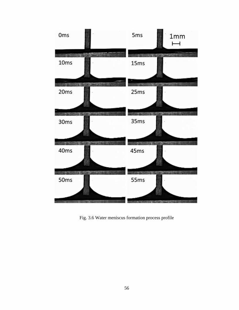
56
Fig. 3.6 Water meniscus formation process profile
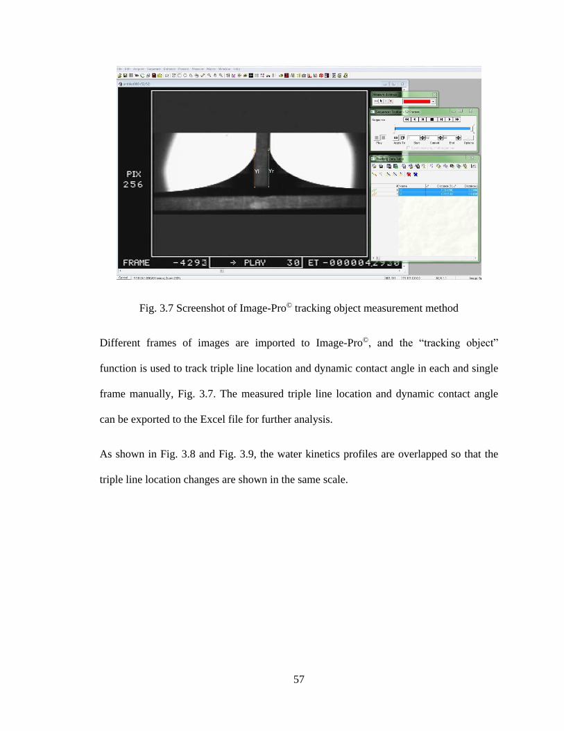
57
Fig. 3.7 Screenshot of Image-Pro© tracking object measurement method
Different frames of images are imported to Image-Pro©, and the “tracking object”
function is used to track triple line location and dynamic contact angle in each and single
frame manually, Fig. 3.7. The measured triple line location and dynamic contact angle
can be exported to the Excel file for further analysis.
As shown in Fig. 3.8 and Fig. 3.9, the water kinetics profiles are overlapped so that the
triple line location changes are shown in the same scale.
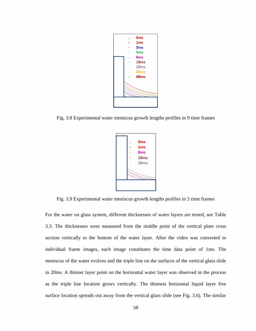
58
Fig. 3.8 Experimental water meniscus growth lengths profiles in 9 time frames
Fig. 3.9 Experimental water meniscus growth lengths profiles in 5 time frames
For the water on glass system, different thicknesses of water layers are tested, see Table
3.3. The thicknesses were measured from the middle point of the vertical plate cross
section vertically to the bottom of the water layer. After the video was converted to
individual frame images, each image constitutes the time data point of 1ms. The
meniscus of the water evolves and the triple line on the surfaces of the vertical glass slide
in 20ms. A thinner layer point on the horizontal water layer was observed in the process
as the triple line location grows vertically. The thinnest horizontal liquid layer free
surface location spreads out away from the vertical glass slide (see Fig. 3.6). The similar
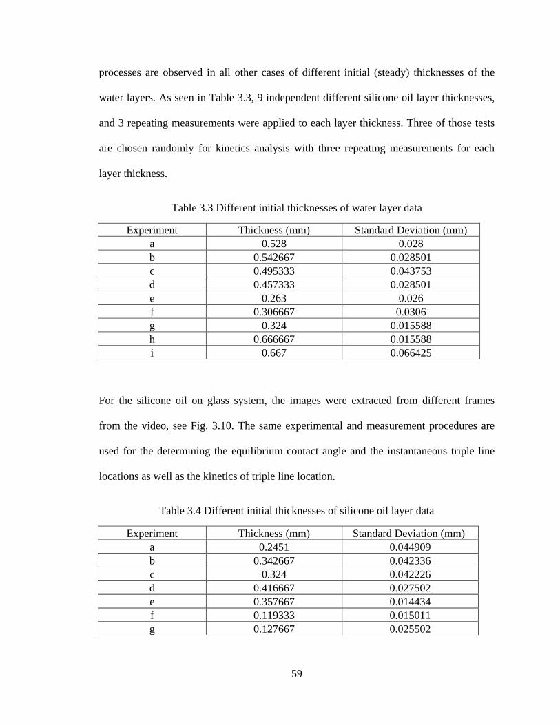
59
processes are observed in all other cases of different initial (steady) thicknesses of the
water layers. As seen in Table 3.3, 9 independent different silicone oil layer thicknesses,
and 3 repeating measurements were applied to each layer thickness. Three of those tests
are chosen randomly for kinetics analysis with three repeating measurements for each
layer thickness.
Table 3.3 Different initial thicknesses of water layer data
Experiment Thickness (mm) Standard Deviation (mm)
a 0.528 0.028
b 0.542667 0.028501
c 0.495333 0.043753
d 0.457333 0.028501
e 0.263 0.026
f 0.306667 0.0306
g 0.324 0.015588
h 0.666667 0.015588
i 0.667 0.066425
For the silicone oil on glass system, the images were extracted from different frames
from the video, see Fig. 3.10. The same experimental and measurement procedures are
used for the determining the equilibrium contact angle and the instantaneous triple line
locations as well as the kinetics of triple line location.
Table 3.4 Different initial thicknesses of silicone oil layer data
Experiment Thickness (mm) Standard Deviation (mm)
a 0.2451 0.044909
b 0.342667 0.042336
c 0.324 0.042226
d 0.416667 0.027502
e 0.357667 0.014434
f 0.119333 0.015011
g 0.127667 0.025502
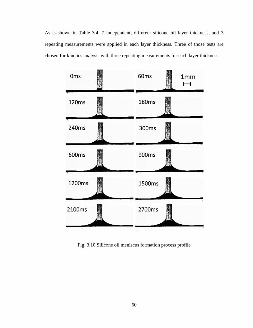
60
As is shown in Table 3.4, 7 independent, different silicone oil layer thickness, and 3
repeating measurements were applied in each layer thickness. Three of those tests are
chosen for kinetics analysis with three repeating measurements for each layer thickness.
Fig. 3.10 Silicone oil meniscus formation process profile
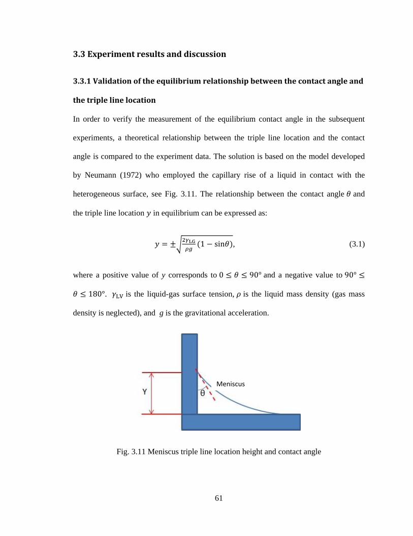
61
3.3 Experiment results and discussion
3.3.1 Validation of the equilibrium relationship between the contact angle and
the triple line location
In order to verify the measurement of the equilibrium contact angle in the subsequent
experiments, a theoretical relationship between the triple line location and the contact
angle is compared to the experiment data. The solution is based on the model developed
by Neumann (1972) who employed the capillary rise of a liquid in contact with the
heterogeneous surface, see Fig. 3.11. The relationship between the contact angle 𝜃 and
the triple line location 𝑦 in equilibrium can be expressed as:
𝑦 = ±√2𝛾LG
𝜌𝑔(1 − sin𝜃), (3.1)
where a positive value of y corresponds to 0 ≤ 𝜃 ≤ 90° and a negative value to 90° ≤
𝜃 ≤ 180°. 𝛾LV is the liquid-gas surface tension, 𝜌 is the liquid mass density (gas mass
density is neglected), and g is the gravitational acceleration.
Fig. 3.11 Meniscus triple line location height and contact angle
Meniscus
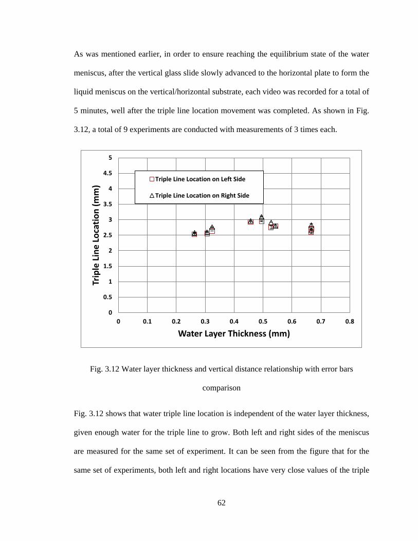
62
As was mentioned earlier, in order to ensure reaching the equilibrium state of the water
meniscus, after the vertical glass slide slowly advanced to the horizontal plate to form the
liquid meniscus on the vertical/horizontal substrate, each video was recorded for a total of
5 minutes, well after the triple line location movement was completed. As shown in Fig.
3.12, a total of 9 experiments are conducted with measurements of 3 times each.
Fig. 3.12 Water layer thickness and vertical distance relationship with error bars
comparison
Fig. 3.12 shows that water triple line location is independent of the water layer thickness,
given enough water for the triple line to grow. Both left and right sides of the meniscus
are measured for the same set of experiment. It can be seen from the figure that for the
same set of experiments, both left and right locations have very close values of the triple
0
0.5
1
1.5
2
2.5
3
3.5
4
4.5
5
0 0.1 0.2 0.3 0.4 0.5 0.6 0.7 0.8
Trip
le L
ine
Lo
cati
on
(m
m)
Water Layer Thickness (mm)
Triple Line Location on Left Side
Triple Line Location on Right Side
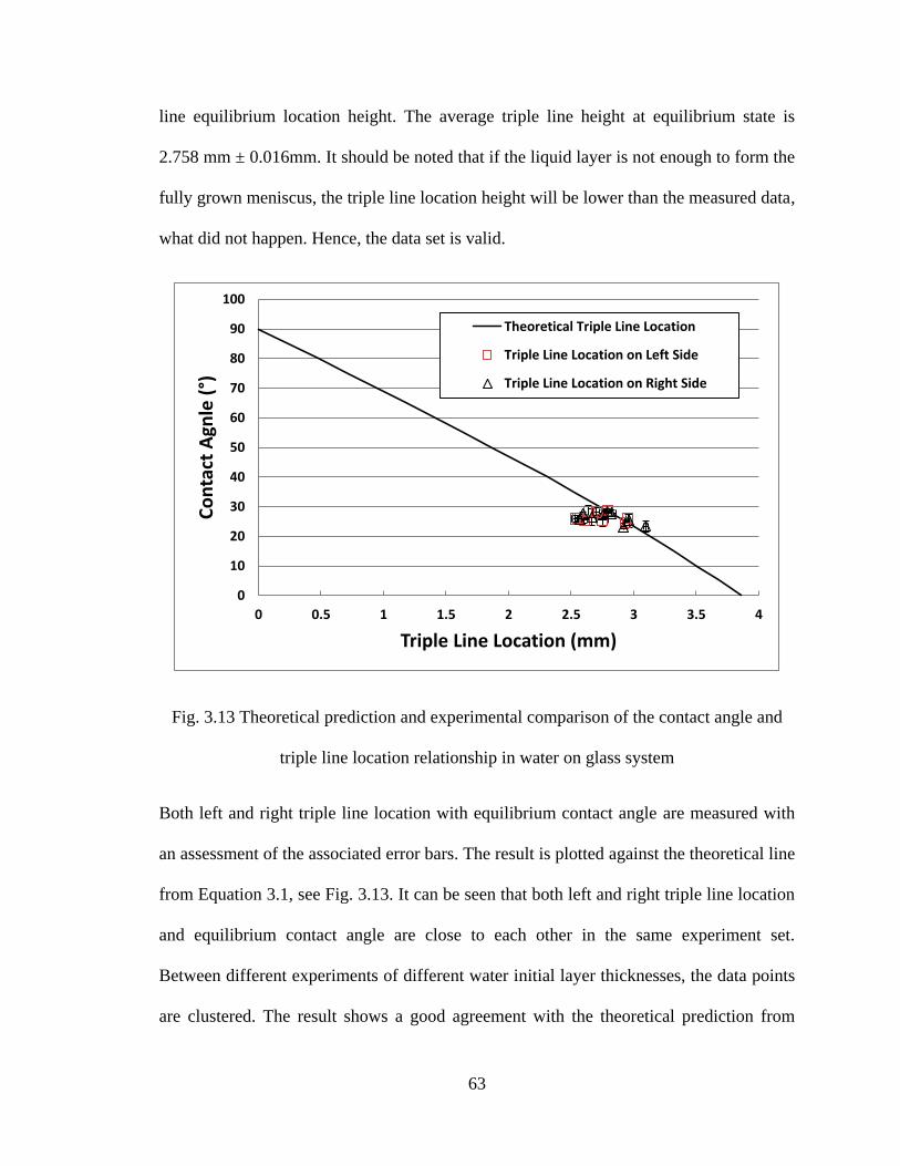
63
line equilibrium location height. The average triple line height at equilibrium state is
2.758 mm ± 0.016mm. It should be noted that if the liquid layer is not enough to form the
fully grown meniscus, the triple line location height will be lower than the measured data,
what did not happen. Hence, the data set is valid.
Fig. 3.13 Theoretical prediction and experimental comparison of the contact angle and
triple line location relationship in water on glass system
Both left and right triple line location with equilibrium contact angle are measured with
an assessment of the associated error bars. The result is plotted against the theoretical line
from Equation 3.1, see Fig. 3.13. It can be seen that both left and right triple line location
and equilibrium contact angle are close to each other in the same experiment set.
Between different experiments of different water initial layer thicknesses, the data points
are clustered. The result shows a good agreement with the theoretical prediction from
0
10
20
30
40
50
60
70
80
90
100
0 0.5 1 1.5 2 2.5 3 3.5 4
Co
nta
ct A
gnle
(°)
Triple Line Location (mm)
Theoretical Triple Line Location
Triple Line Location on Left Side
Triple Line Location on Right Side
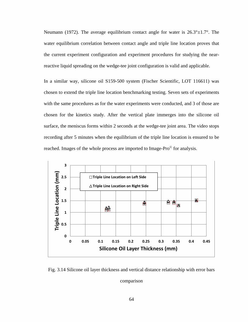
64
Neumann (1972). The average equilibrium contact angle for water is 26.3°±1.7°. The
water equilibrium correlation between contact angle and triple line location proves that
the current experiment configuration and experiment procedures for studying the near-
reactive liquid spreading on the wedge-tee joint configuration is valid and applicable.
In a similar way, silicone oil S159-500 system (Fischer Scientific, LOT 116611) was
chosen to extend the triple line location benchmarking testing. Seven sets of experiments
with the same procedures as for the water experiments were conducted, and 3 of those are
chosen for the kinetics study. After the vertical plate immerges into the silicone oil
surface, the meniscus forms within 2 seconds at the wedge-tee joint area. The video stops
recording after 5 minutes when the equilibrium of the triple line location is ensured to be
reached. Images of the whole process are imported to Image-Pro© for analysis.
Fig. 3.14 Silicone oil layer thickness and vertical distance relationship with error bars
comparison
0
0.5
1
1.5
2
2.5
3
0 0.05 0.1 0.15 0.2 0.25 0.3 0.35 0.4 0.45
Trip
le L
ine
Lo
cati
on
(m
m)
Silicone Oil Layer Thickness (mm)
Triple Line Location on Left Side
Triple Line Location on Right Side
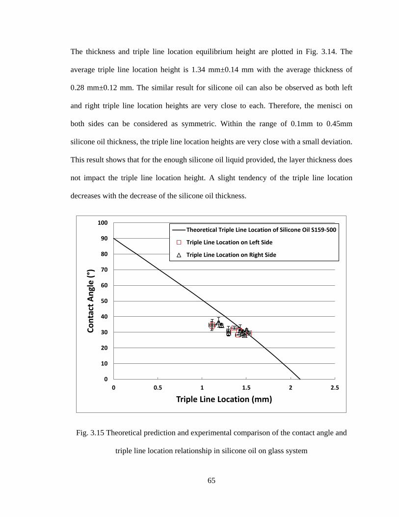
65
The thickness and triple line location equilibrium height are plotted in Fig. 3.14. The
average triple line location height is 1.34 mm±0.14 mm with the average thickness of
0.28 mm±0.12 mm. The similar result for silicone oil can also be observed as both left
and right triple line location heights are very close to each. Therefore, the menisci on
both sides can be considered as symmetric. Within the range of 0.1mm to 0.45mm
silicone oil thickness, the triple line location heights are very close with a small deviation.
This result shows that for the enough silicone oil liquid provided, the layer thickness does
not impact the triple line location height. A slight tendency of the triple line location
decreases with the decrease of the silicone oil thickness.
Fig. 3.15 Theoretical prediction and experimental comparison of the contact angle and
triple line location relationship in silicone oil on glass system
0
10
20
30
40
50
60
70
80
90
100
0 0.5 1 1.5 2 2.5
Co
nta
ct A
ngl
e (
°)
Triple Line Location (mm)
Theoretical Triple Line Location of Silicone Oil S159-500
Triple Line Location on Left Side
Triple Line Location on Right Side
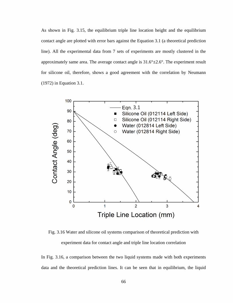
66
As shown in Fig. 3.15, the equilibrium triple line location height and the equilibrium
contact angle are plotted with error bars against the Equation 3.1 (a theoretical prediction
line). All the experimental data from 7 sets of experiments are mostly clustered in the
approximately same area. The average contact angle is 31.6°±2.6°. The experiment result
for silicone oil, therefore, shows a good agreement with the correlation by Neumann
(1972) in Equation 3.1.
Fig. 3.16 Water and silicone oil systems comparison of theoretical prediction with
experiment data for contact angle and triple line location correlation
In Fig. 3.16, a comparison between the two liquid systems made with both experiments
data and the theoretical prediction lines. It can be seen that in equilibrium, the liquid
67
systems fully agree with the traditional Young-Neumann theory and verify fully the
agreement with the experimental data. Note again that multiple experiments were
conducted in each system case on both left and right sides of the joint zone, and multiple
measurements were taken to minimize the errors potentially caused during the
measurement procedure. The generated data sets show the consistency regardless of
different liquid layer thicknesses with small standard deviations. Hence, the theoretical
and experimental results agreement is satisfactorily verified and the validity of the
measurements of the contact angle and the triple line location has been established.
3.3.2 Dynamic contact angle experimental correlation
As mentioned in Chapter 2, many sources have reported the relationships between
dynamic contact angle and the capillary number (𝐶𝑎 =𝜇𝑈
𝛾 , µ is the liquid viscosity, 𝛾 is
the liquid surface tension and U is the triple line movement speed). Jiang et al. (1979)
proposed an empirical, universal function for the model, applicable for silicone type of
liquid at the ambient temperature:
𝑐𝑜𝑠 𝜃 −𝑐𝑜𝑠 𝜃(𝑡)
𝑐𝑜𝑠 𝜃+1= 𝑡𝑎𝑛ℎ(4.96𝐶𝑎0.702) (3.2)
where 𝜃 is the static contact angle, 𝜃(𝑡) is the dynamic contact angle.
Similar empirical models were also reported by Brake et al. (1973) and Seeberg et al.
(1992). Seebergh et al. (1992) found that the models have a good agreement for high
capillary numbers (10−3 ≤ 𝐶𝑎 ≤ 3 ∙ 10−2), but not for low capillary numbers. In our
case, the water system capillary number is low enough to be considered as the capillary
number. The functions are expressed as follows (Seebergh et al., 1992):
68
𝑐𝑜𝑠 𝜃 −𝑐𝑜𝑠 𝜃(𝑡)
𝑐𝑜𝑠 𝜃+1= 2.24𝐶𝑎0.54 (3.3a)
for 𝐶𝑎 ≤ 10−3, 𝑐𝑜𝑠 𝜃 −𝑐𝑜𝑠 𝜃(𝑡)
𝑐𝑜𝑠 𝜃+1= 4.47𝐶𝑎0.42 (3.3b)
Due to the fact that both left and right side of the menisci are close to each other, see Fig.
3.16, presenting a symmetric trend, to clearly show the total set of experiment data, both
of left side and the right side of the two menisci were chosen to compare with the
empirical correlations. The linear scale comparison of the experiment data and Jiang’s
(1979) empirical correlation shows good agreement. As shown in Fig. 3.17, the
experiment data only presents dynamic contact angle from 20° to 60°, this is only
partially covered in the empirical correlation. This result can be explained by the
limitation of the current Wilhelmy plate configuration, see Fig. 3.18. The last dynamic
contact angle is always larger than the equilibrium contact angle of the specific liquid
system, whereas the initial contact angle is never larger than 90°.
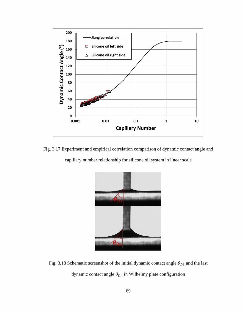
69
Fig. 3.17 Experiment and empirical correlation comparison of dynamic contact angle and
capillary number relationship for silicone oil system in linear scale
Fig. 3.18 Schematic screenshot of the initial dynamic contact angle 𝜃𝐷1 and the last
dynamic contact angle 𝜃𝐷𝑛 in Wilhelmy plate configuration
0
20
40
60
80
100
120
140
160
180
200
0.001 0.01 0.1 1 10
Dyn
amic
Co
nta
ct A
ngl
e (
°)
Capillary Number
Jiang correlation
Silicone oil left side
Silicone oil right side
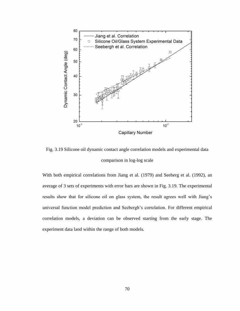
70
Fig. 3.19 Silicone oil dynamic contact angle correlation models and experimental data
comparison in log-log scale
With both empirical correlations from Jiang et al. (1979) and Seeberg et al. (1992), an
average of 3 sets of experiments with error bars are shown in Fig. 3.19. The experimental
results show that for silicone oil on glass system, the result agrees well with Jiang’s
universal function model prediction and Seebergh’s correlation. For different empirical
correlation models, a deviation can be observed starting from the early stage. The
experiment data land within the range of both models.
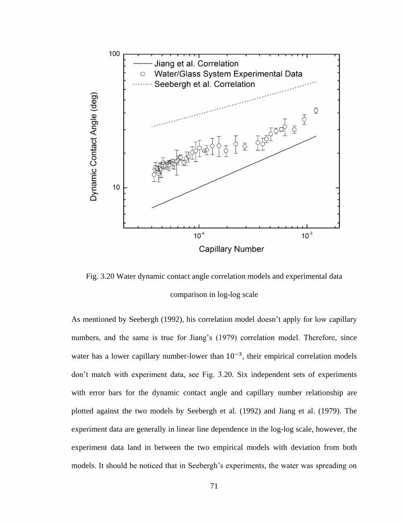
71
Fig. 3.20 Water dynamic contact angle correlation models and experimental data
comparison in log-log scale
As mentioned by Seebergh (1992), his correlation model doesn’t apply for low capillary
numbers, and the same is true for Jiang’s (1979) correlation model. Therefore, since
water has a lower capillary number-lower than 10−3, their empirical correlation models
don’t match with experiment data, see Fig. 3.20. Six independent sets of experiments
with error bars for the dynamic contact angle and capillary number relationship are
plotted against the two models by Seebergh et al. (1992) and Jiang et al. (1979). The
experiment data are generally in linear line dependence in the log-log scale, however, the
experiment data land in between the two empirical models with deviation from both
models. It should be noticed that in Seebergh’s experiments, the water was spreading on
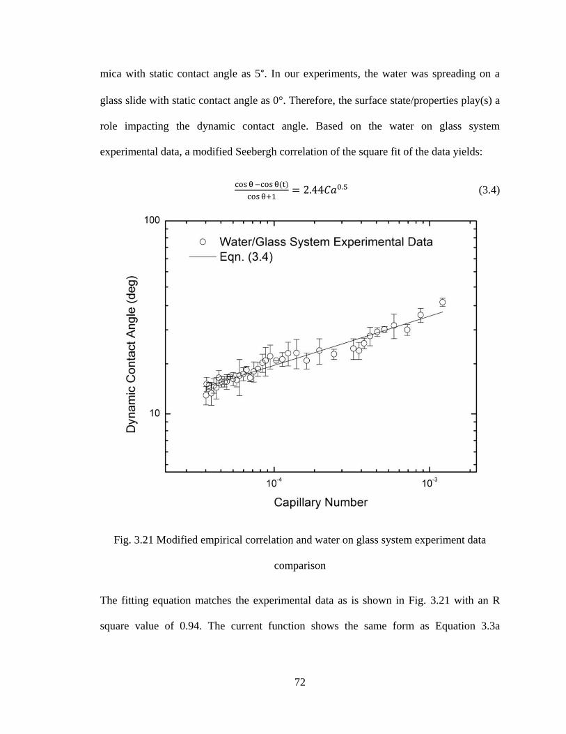
72
mica with static contact angle as 5°. In our experiments, the water was spreading on a
glass slide with static contact angle as 0°. Therefore, the surface state/properties play(s) a
role impacting the dynamic contact angle. Based on the water on glass system
experimental data, a modified Seebergh correlation of the square fit of the data yields:
cos θ −cos θ(t)
cos θ+1= 2.44𝐶𝑎0.5 (3.4)
Fig. 3.21 Modified empirical correlation and water on glass system experiment data
comparison
The fitting equation matches the experimental data as is shown in Fig. 3.21 with an R
square value of 0.94. The current function shows the same form as Equation 3.3a
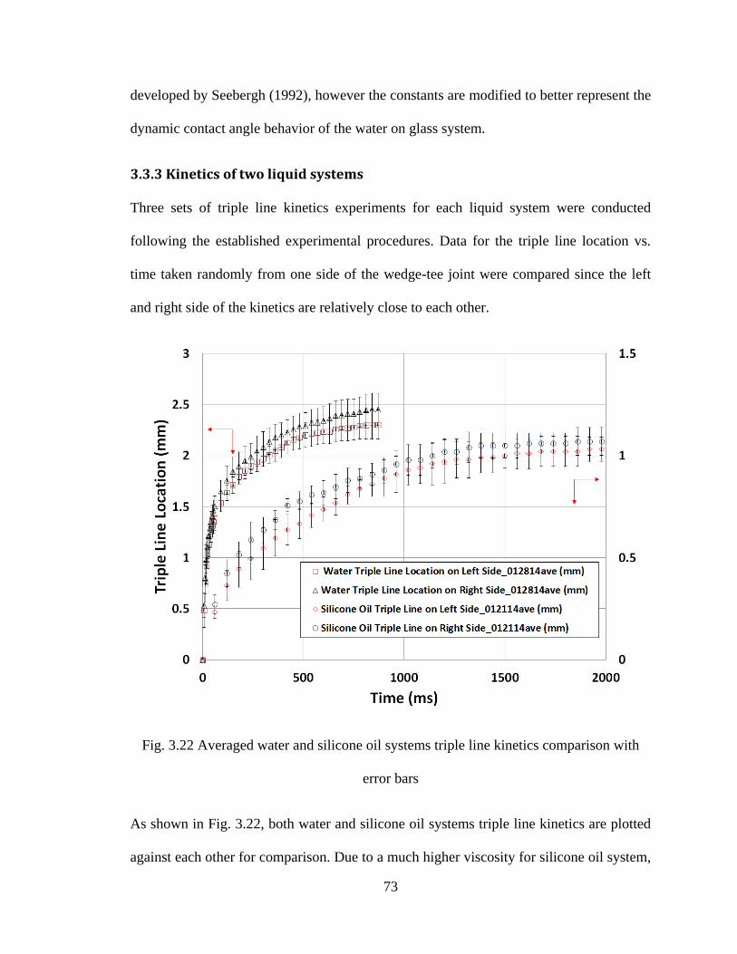
73
developed by Seebergh (1992), however the constants are modified to better represent the
dynamic contact angle behavior of the water on glass system.
3.3.3 Kinetics of two liquid systems
Three sets of triple line kinetics experiments for each liquid system were conducted
following the established experimental procedures. Data for the triple line location vs.
time taken randomly from one side of the wedge-tee joint were compared since the left
and right side of the kinetics are relatively close to each other.
Fig. 3.22 Averaged water and silicone oil systems triple line kinetics comparison with
error bars
As shown in Fig. 3.22, both water and silicone oil systems triple line kinetics are plotted
against each other for comparison. Due to a much higher viscosity for silicone oil system,
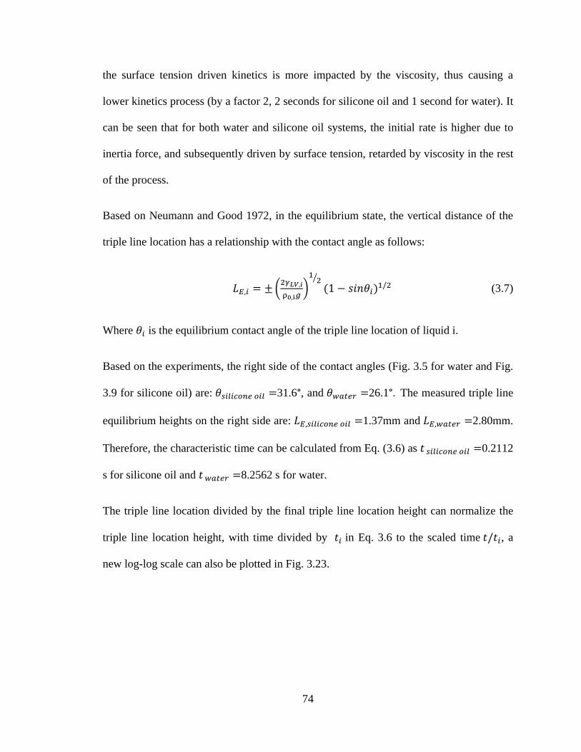
74
the surface tension driven kinetics is more impacted by the viscosity, thus causing a
lower kinetics process (by a factor 2, 2 seconds for silicone oil and 1 second for water). It
can be seen that for both water and silicone oil systems, the initial rate is higher due to
inertia force, and subsequently driven by surface tension, retarded by viscosity in the rest
of the process.
Based on Neumann and Good 1972, in the equilibrium state, the vertical distance of the
triple line location has a relationship with the contact angle as follows:
𝐿𝐸,𝑖 = ± (2𝛾𝐿𝑉,𝑖
ρ0,i𝑔)
12⁄
(1 − 𝑠𝑖𝑛𝜃𝑖)1/2 (3.7)
Where 𝜃𝑖 is the equilibrium contact angle of the triple line location of liquid i.
Based on the experiments, the right side of the contact angles (Fig. 3.5 for water and Fig.
3.9 for silicone oil) are: 𝜃𝑠𝑖𝑙𝑖𝑐𝑜𝑛𝑒 𝑜𝑖𝑙 =31.6°, and 𝜃𝑤𝑎𝑡𝑒𝑟 =26.1°. The measured triple line
equilibrium heights on the right side are: 𝐿𝐸,𝑠𝑖𝑙𝑖𝑐𝑜𝑛𝑒 𝑜𝑖𝑙 =1.37mm and 𝐿𝐸,𝑤𝑎𝑡𝑒𝑟 =2.80mm.
Therefore, the characteristic time can be calculated from Eq. (3.6) as 𝑡 𝑠𝑖𝑙𝑖𝑐𝑜𝑛𝑒 𝑜𝑖𝑙 =0.2112
s for silicone oil and 𝑡 𝑤𝑎𝑡𝑒𝑟 =8.2562 s for water.
The triple line location divided by the final triple line location height can normalize the
triple line location height, with time divided by 𝑡𝑖 in Eq. 3.6 to the scaled time 𝑡/𝑡𝑖, a
new log-log scale can also be plotted in Fig. 3.23.
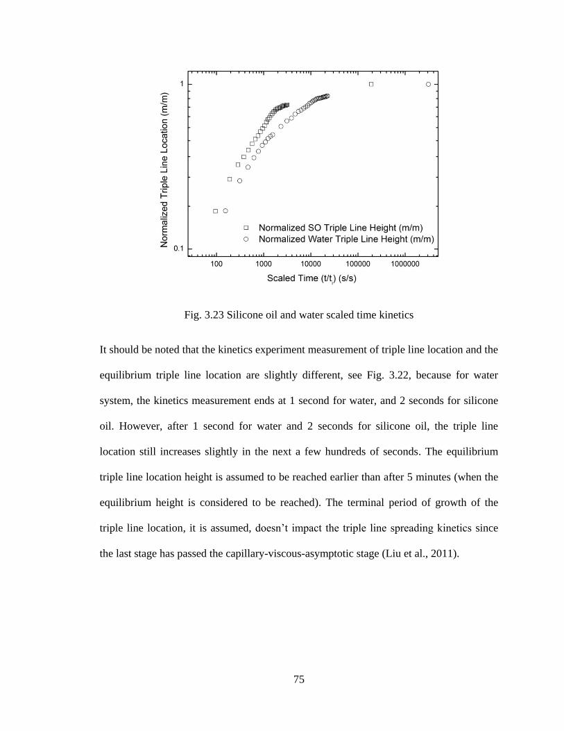
75
Fig. 3.23 Silicone oil and water scaled time kinetics
It should be noted that the kinetics experiment measurement of triple line location and the
equilibrium triple line location are slightly different, see Fig. 3.22, because for water
system, the kinetics measurement ends at 1 second for water, and 2 seconds for silicone
oil. However, after 1 second for water and 2 seconds for silicone oil, the triple line
location still increases slightly in the next a few hundreds of seconds. The equilibrium
triple line location height is assumed to be reached earlier than after 5 minutes (when the
equilibrium height is considered to be reached). The terminal period of growth of the
triple line location, it is assumed, doesn’t impact the triple line spreading kinetics since
the last stage has passed the capillary-viscous-asymptotic stage (Liu et al., 2011).
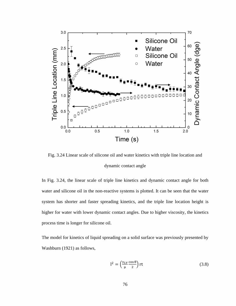
76
Fig. 3.24 Linear scale of silicone oil and water kinetics with triple line location and
dynamic contact angle
In Fig. 3.24, the linear scale of triple line kinetics and dynamic contact angle for both
water and silicone oil in the non-reactive systems is plotted. It can be seen that the water
system has shorter and faster spreading kinetics, and the triple line location height is
higher for water with lower dynamic contact angles. Due to higher viscosity, the kinetics
process time is longer for silicone oil.
The model for kinetics of liquid spreading on a solid surface was previously presented by
Washburn (1921) as follows,
l2 = (γLV
μ
cos θ
2) rt (3.8)
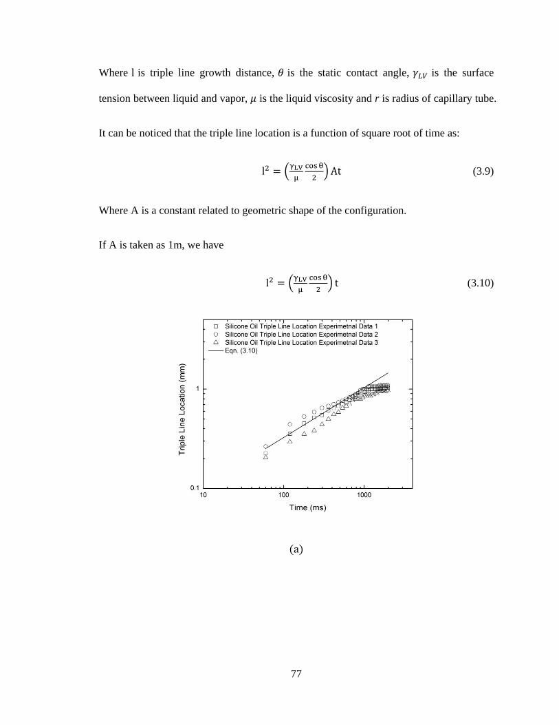
77
Where l is triple line growth distance, 𝜃 is the static contact angle, 𝛾𝐿𝑉 is the surface
tension between liquid and vapor, 𝜇 is the liquid viscosity and r is radius of capillary tube.
It can be noticed that the triple line location is a function of square root of time as:
l2 = (γLV
μ
cos θ
2) At (3.9)
Where A is a constant related to geometric shape of the configuration.
If A is taken as 1m, we have
l2 = (γLV
μ
cos θ
2) t (3.10)
(a)
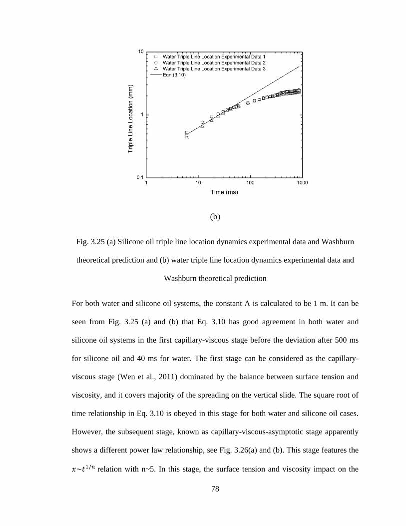
78
(b)
Fig. 3.25 (a) Silicone oil triple line location dynamics experimental data and Washburn
theoretical prediction and (b) water triple line location dynamics experimental data and
Washburn theoretical prediction
For both water and silicone oil systems, the constant A is calculated to be 1 m. It can be
seen from Fig. 3.25 (a) and (b) that Eq. 3.10 has good agreement in both water and
silicone oil systems in the first capillary-viscous stage before the deviation after 500 ms
for silicone oil and 40 ms for water. The first stage can be considered as the capillary-
viscous stage (Wen et al., 2011) dominated by the balance between surface tension and
viscosity, and it covers majority of the spreading on the vertical slide. The square root of
time relationship in Eq. 3.10 is obeyed in this stage for both water and silicone oil cases.
However, the subsequent stage, known as capillary-viscous-asymptotic stage apparently
shows a different power law relationship, see Fig. 3.26(a) and (b). This stage features the
𝑥~𝑡1/𝑛 relation with n~5. In this stage, the surface tension and viscosity impact on the
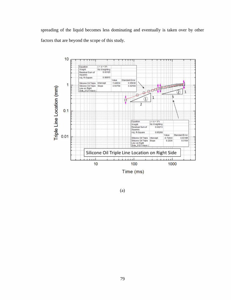
79
spreading of the liquid becomes less dominating and eventually is taken over by other
factors that are beyond the scope of this study.
(a)
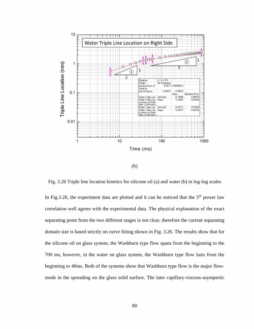
80
(b)
Fig. 3.26 Triple line location kinetics for silicone oil (a) and water (b) in log-log scales
In Fig.3.26, the experiment data are plotted and it can be noticed that the 5th power law
correlation well agrees with the experimental data. The physical explanation of the exact
separating point from the two different stages is not clear, therefore the current separating
domain size is based strictly on curve fitting shown in Fig. 3.26. The results show that for
the silicone oil on glass system, the Washburn type flow spans from the beginning to the
700 ms, however, in the water on glass system, the Washburn type flow lasts from the
beginning to 40ms. Both of the systems show that Washburn type flow is the major flow-
mode in the spreading on the glass solid surface. The later capillary-viscous-asymptotic
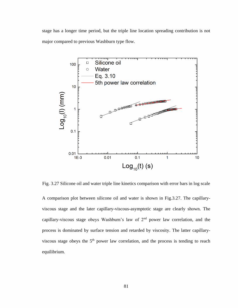
81
stage has a longer time period, but the triple line location spreading contribution is not
major compared to previous Washburn type flow.
Fig. 3.27 Silicone oil and water triple line kinetics comparison with error bars in log scale
A comparison plot between silicone oil and water is shown in Fig.3.27. The capillary-
viscous stage and the later capillary-viscous-asymptotic stage are clearly shown. The
capillary-viscous stage obeys Washburn’s law of 2nd power law correlation, and the
process is dominated by surface tension and retarded by viscosity. The latter capillary-
viscous stage obeys the 5th power law correlation, and the process is tending to reach
equilibrium.
82
3.4 Summary
In this chapter, the benchmark experiments of non-reactive liquid wetting systems at low
temperatures are presented in a process of designing the experimental methodology for
experiments on reactive wetting at elevated temperatures. The benchmark experiment
results also serve the purpose of a tool to verify the numerical simulation that is funded
by the same collaborative NSF project with the team at the Washington State University
(Grant CBET # 1234581 and 1235759).
Two common non-reactive liquid-substrates are used. The liquids spread over the glass
wedge-tee configuration to simulate the joint formation configuration to be used for the
reactive wetting at elevated temperatures. To establish the reliable database for the non-
reactive wetting kinetics, a wetting experiment is adopted to validate the experiment
configuration and procedures. In the wetting experiment, the contact angle and the
equilibrium triple line location relationship was verified and compared with theoretical
results. The experiment data show good agreement with the theoretical prediction for
both water and silicone oil systems. The experiment result also shows at a certain given
range of liquid layer thicknesses, the triple line location equilibrium height is independent
from the liquid thickness. In the kinetics segment of experiments, silicone oil dynamic
contact angle and capillary length can agree with the theoretical correlation. The water
dynamic contact angle and triple line location correlation feature a deviation when
compared to some existing correlations developed earlier and reported in literature. A
new modified correlation for water dynamic contact angle and capillary number
correlation was established for the water on glass system. The liquid systems wetting also
obey the classic Washburn flow model in the capillary-viscous stage, showing the initial
83
wetting is mainly impacted by surface tension and viscosity. The subsequent capillary-
viscous-asymptotic stage shows that for these two liquid systems, a 5th power law
correlation can easily be identified. The experiment data error analysis is performed (see
associated Appendix A) to explore the potential main causes of data dispersion. The
result shows the vertical plate movement of the Wilhelmy plate configuration is having
little impact on the triple line kinetics experiment data. The measurement error
contributes to a smaller degree to the overall error level compared to the experimental
conditions, namely the glass plate surface condition variations and environmental
conditions.
84
CHAPTER 4: EXPERIMENTAL EQUIPMENT AND
PROCEDURES FOR THE HIGH TEMPERATURE CAPILLARY
FLOW STUDY
4.1 Overview
Chapter 4 is mainly focused on the experiment preparation, equipment and procedures for
the reactive wetting at elevated temperatures. As mentioned in Chapter 2, sessile drop
experiment method is a major method to investigate the liquid spreading and wetting
phenomena due to its simplicity and yet thoroughly coverage of both contact angle and
triple line location behavior. The experiment preparation and procedures introduced in
this chapter offer general guidelines of the preparation method and procedures for
experiments presented in later chapters. Various experiments will involve different
sample designs, preparations and procedures, but the overall intention of all the
experiments is to generate data for a study of the molten metal spreading at high
temperatures with the same experiment equipment and its accessories.
The Optical Contact Angle Analyzer (OCA) is the main piece of equipment used in the
molten metal spreading research. It is assembled in the Brazing, soldering and heat
exchangers research laboratory at the Institute of Sustainable Manufacturing at
University of Kentucky. Other experiment facilities include scanning electron microscope
(SEM), optical surface profiler, and differential scanning calorimeter (DSC) at University
of Kentucky.
Typical sample design and preparation examples will be illustrated in this chapter along
with the corresponding general experiment procedures. Post-experiment samples
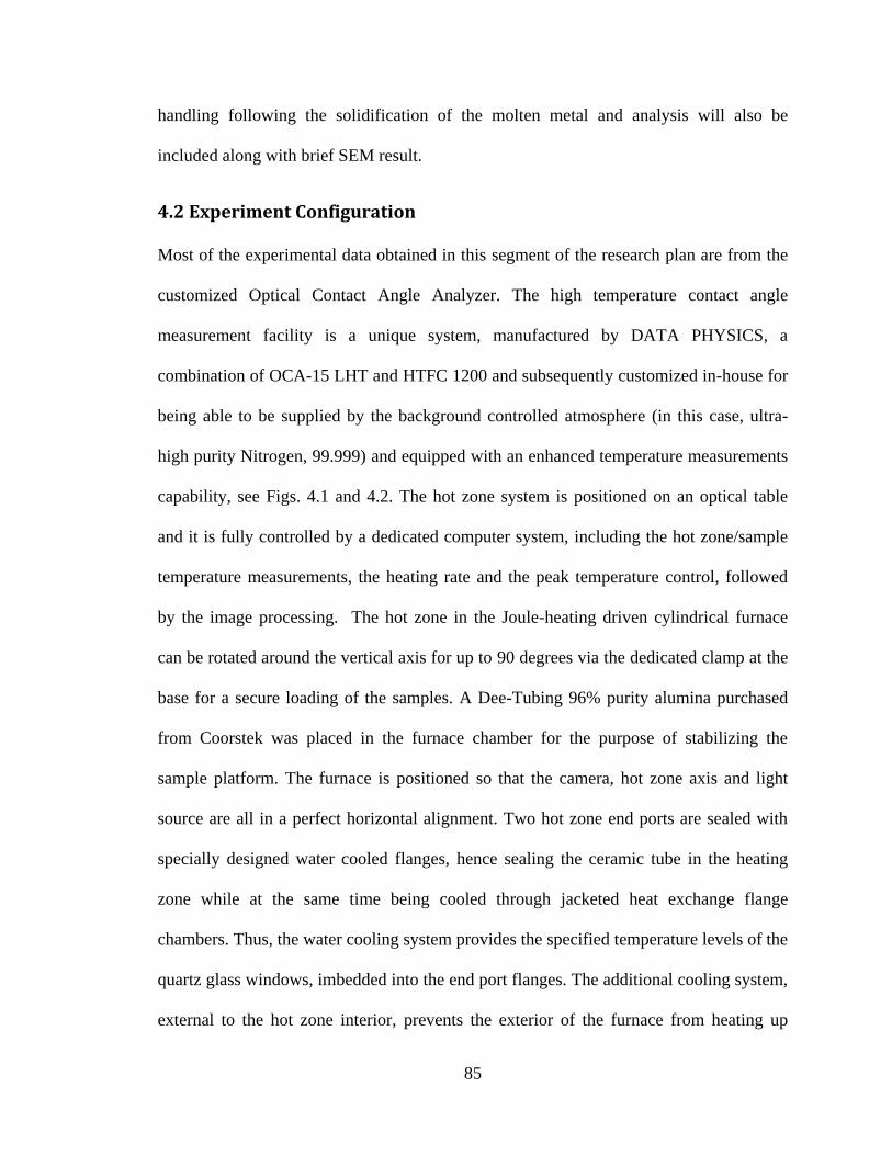
85
handling following the solidification of the molten metal and analysis will also be
included along with brief SEM result.
4.2 Experiment Configuration
Most of the experimental data obtained in this segment of the research plan are from the
customized Optical Contact Angle Analyzer. The high temperature contact angle
measurement facility is a unique system, manufactured by DATA PHYSICS, a
combination of OCA-15 LHT and HTFC 1200 and subsequently customized in-house for
being able to be supplied by the background controlled atmosphere (in this case, ultra-
high purity Nitrogen, 99.999) and equipped with an enhanced temperature measurements
capability, see Figs. 4.1 and 4.2. The hot zone system is positioned on an optical table
and it is fully controlled by a dedicated computer system, including the hot zone/sample
temperature measurements, the heating rate and the peak temperature control, followed
by the image processing. The hot zone in the Joule-heating driven cylindrical furnace
can be rotated around the vertical axis for up to 90 degrees via the dedicated clamp at the
base for a secure loading of the samples. A Dee-Tubing 96% purity alumina purchased
from Coorstek was placed in the furnace chamber for the purpose of stabilizing the
sample platform. The furnace is positioned so that the camera, hot zone axis and light
source are all in a perfect horizontal alignment. Two hot zone end ports are sealed with
specially designed water cooled flanges, hence sealing the ceramic tube in the heating
zone while at the same time being cooled through jacketed heat exchange flange
chambers. Thus, the water cooling system provides the specified temperature levels of the
quartz glass windows, imbedded into the end port flanges. The additional cooling system,
external to the hot zone interior, prevents the exterior of the furnace from heating up
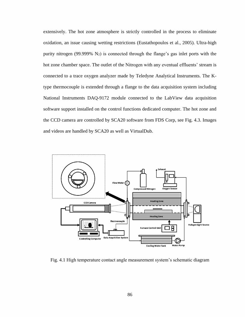
86
extensively. The hot zone atmosphere is strictly controlled in the process to eliminate
oxidation, an issue causing wetting restrictions (Eustathopoulos et al., 2005). Ultra-high
purity nitrogen (99.999% N2) is connected through the flange’s gas inlet ports with the
hot zone chamber space. The outlet of the Nitrogen with any eventual effluents’ stream is
connected to a trace oxygen analyzer made by Teledyne Analytical Instruments. The K-
type thermocouple is extended through a flange to the data acquisition system including
National Instruments DAQ-9172 module connected to the LabView data acquisition
software support installed on the control functions dedicated computer. The hot zone and
the CCD camera are controlled by SCA20 software from FDS Corp, see Fig. 4.3. Images
and videos are handled by SCA20 as well as VirtualDub.
Fig. 4.1 High temperature contact angle measurement system’s schematic diagram
87
Fig. 4.2 OCA system facility
1-CCD camera 2-Bubble level 3-Frame 4-Quartz glass window (Left) 5-Purging gas
inlet valve 6-External thermocouple 7 -Flange water cooling inlet (Left) 8-Flange water
cooling outlet (Left) 9-Thermally conductive ceramics tube 10-Furnace top cover water
cooling outlet 11-Furnace 12-Hot zone/Sample location (Inside) 13-Furnace rotation
knob 14-Furnace top cover water cooling inlet 15-Flange water cooling outlet (Right) 16
-Flange water cooling inlet (Right) 17-Exhaust gas outlet pipe 18-Quartz glass window
(Right) 19-Halogen light 20-External USB ports 21-Built-in thermocouple
As shown in Fig. 4.2, the high temperature furnace (designation 11, operational up to
1700 K) has the inner diameter of 35 mm and length of 300 mm so that it can easily
accommodate a single test sample at a time. The hot zone (12) is visually unobstructed in
the axial direction (4-18) except for the presence of the test specimen and its supporting
structure. A halogen light source (19) delivers a homogeneous visible light flux and is
located on one side (a far-end) of the hot zone to illuminate the ceramic inner tube space,
obstructed from the field of vision of the front camera only by a test sample contour. So,
88
the sample’s side shade view is visible from the opposite side of the hot zone as a black
contour image on a white background. Additional ports for the background atmosphere
gas supply and exhaust exits are included (5 and 17). Transparent side windows allow on
one side an access to the light source illuminating the hot zone, and on the other side to a
telescope (1) for digital camera recording of the shadow image. The two flanges are
sealing the ceramic tube of the heating zone and are also cooled by the water cooling
system (7.8 and 15, 16). This cooling system prevents the exterior of the oven, as well as
the lateral windows ports, from an excessive heating. The temperature ramping speed can
be controlled by SCA20 by setting different temperature ramps, see Fig. 4.4. The
maximum temperature ramp can be reached by the hot zone is 40°C/min. It should be
noted that SCA20 doesn’t have the limit of temperature information. Thus by setting the
temperature heating rate higher than 40°C/min could only result in 40°C/min of heating
rate in the physical heat zone by the heaters. The default heating rate by the system is also
40°C/min as tested by various experiments.
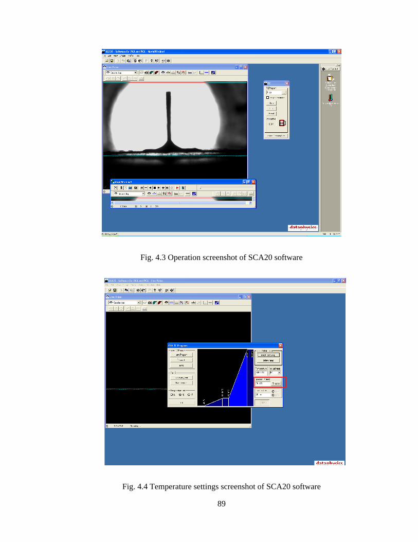
89
Fig. 4.3 Operation screenshot of SCA20 software
Fig. 4.4 Temperature settings screenshot of SCA20 software
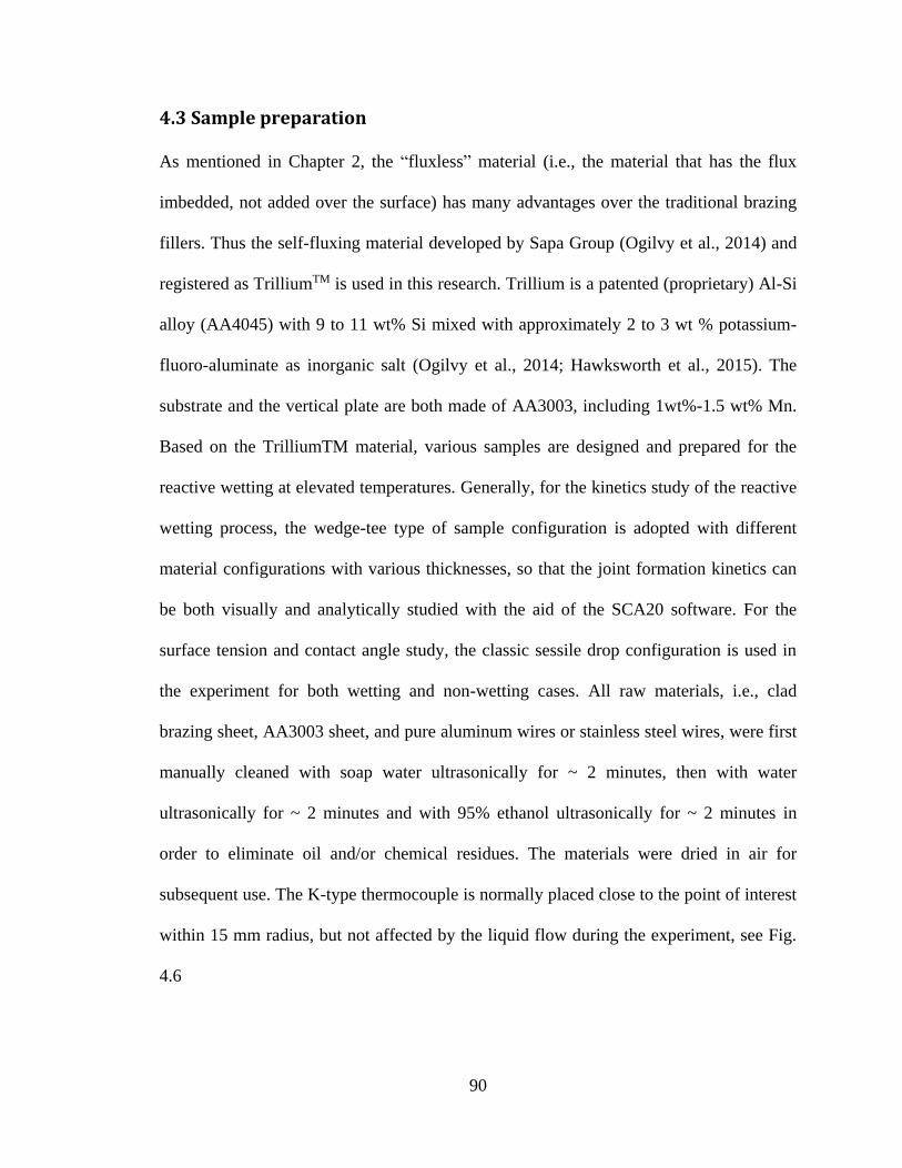
90
4.3 Sample preparation
As mentioned in Chapter 2, the “fluxless” material (i.e., the material that has the flux
imbedded, not added over the surface) has many advantages over the traditional brazing
fillers. Thus the self-fluxing material developed by Sapa Group (Ogilvy et al., 2014) and
registered as TrilliumTM is used in this research. Trillium is a patented (proprietary) Al-Si
alloy (AA4045) with 9 to 11 wt% Si mixed with approximately 2 to 3 wt % potassium-
fluoro-aluminate as inorganic salt (Ogilvy et al., 2014; Hawksworth et al., 2015). The
substrate and the vertical plate are both made of AA3003, including 1wt%-1.5 wt% Mn.
Based on the TrilliumTM material, various samples are designed and prepared for the
reactive wetting at elevated temperatures. Generally, for the kinetics study of the reactive
wetting process, the wedge-tee type of sample configuration is adopted with different
material configurations with various thicknesses, so that the joint formation kinetics can
be both visually and analytically studied with the aid of the SCA20 software. For the
surface tension and contact angle study, the classic sessile drop configuration is used in
the experiment for both wetting and non-wetting cases. All raw materials, i.e., clad
brazing sheet, AA3003 sheet, and pure aluminum wires or stainless steel wires, were first
manually cleaned with soap water ultrasonically for ~ 2 minutes, then with water
ultrasonically for ~ 2 minutes and with 95% ethanol ultrasonically for ~ 2 minutes in
order to eliminate oil and/or chemical residues. The materials were dried in air for
subsequent use. The K-type thermocouple is normally placed close to the point of interest
within 15 mm radius, but not affected by the liquid flow during the experiment, see Fig.
4.6
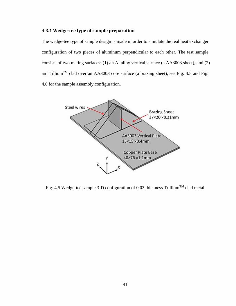
91
4.3.1 Wedge-tee type of sample preparation
The wedge-tee type of sample design is made in order to simulate the real heat exchanger
configuration of two pieces of aluminum perpendicular to each other. The test sample
consists of two mating surfaces: (1) an Al alloy vertical surface (a AA3003 sheet), and (2)
an TrilliumTM clad over an AA3003 core surface (a brazing sheet), see Fig. 4.5 and Fig.
4.6 for the sample assembly configuration.
Fig. 4.5 Wedge-tee sample 3-D configuration of 0.03 thickness TrilliumTM clad metal
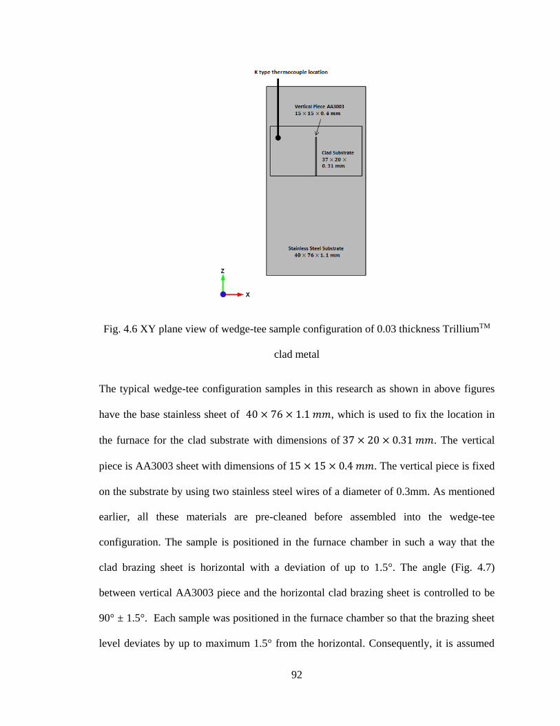
92
Fig. 4.6 XY plane view of wedge-tee sample configuration of 0.03 thickness TrilliumTM
clad metal
The typical wedge-tee configuration samples in this research as shown in above figures
have the base stainless sheet of 40 × 76 × 1.1 𝑚𝑚, which is used to fix the location in
the furnace for the clad substrate with dimensions of 37 × 20 × 0.31 𝑚𝑚. The vertical
piece is AA3003 sheet with dimensions of 15 × 15 × 0.4 𝑚𝑚. The vertical piece is fixed
on the substrate by using two stainless steel wires of a diameter of 0.3mm. As mentioned
earlier, all these materials are pre-cleaned before assembled into the wedge-tee
configuration. The sample is positioned in the furnace chamber in such a way that the
clad brazing sheet is horizontal with a deviation of up to 1.5°. The angle (Fig. 4.7)
between vertical AA3003 piece and the horizontal clad brazing sheet is controlled to be
90° ± 1.5°. Each sample was positioned in the furnace chamber so that the brazing sheet
level deviates by up to maximum 1.5° from the horizontal. Consequently, it is assumed
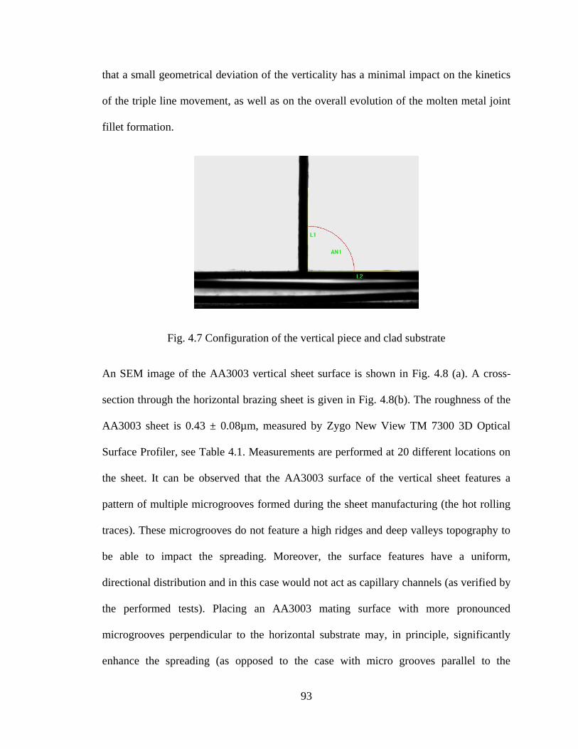
93
that a small geometrical deviation of the verticality has a minimal impact on the kinetics
of the triple line movement, as well as on the overall evolution of the molten metal joint
fillet formation.
Fig. 4.7 Configuration of the vertical piece and clad substrate
An SEM image of the AA3003 vertical sheet surface is shown in Fig. 4.8 (a). A cross-
section through the horizontal brazing sheet is given in Fig. 4.8(b). The roughness of the
AA3003 sheet is 0.43 ± 0.08µm, measured by Zygo New View TM 7300 3D Optical
Surface Profiler, see Table 4.1. Measurements are performed at 20 different locations on
the sheet. It can be observed that the AA3003 surface of the vertical sheet features a
pattern of multiple microgrooves formed during the sheet manufacturing (the hot rolling
traces). These microgrooves do not feature a high ridges and deep valleys topography to
be able to impact the spreading. Moreover, the surface features have a uniform,
directional distribution and in this case would not act as capillary channels (as verified by
the performed tests). Placing an AA3003 mating surface with more pronounced
microgrooves perpendicular to the horizontal substrate may, in principle, significantly
enhance the spreading (as opposed to the case with micro grooves parallel to the
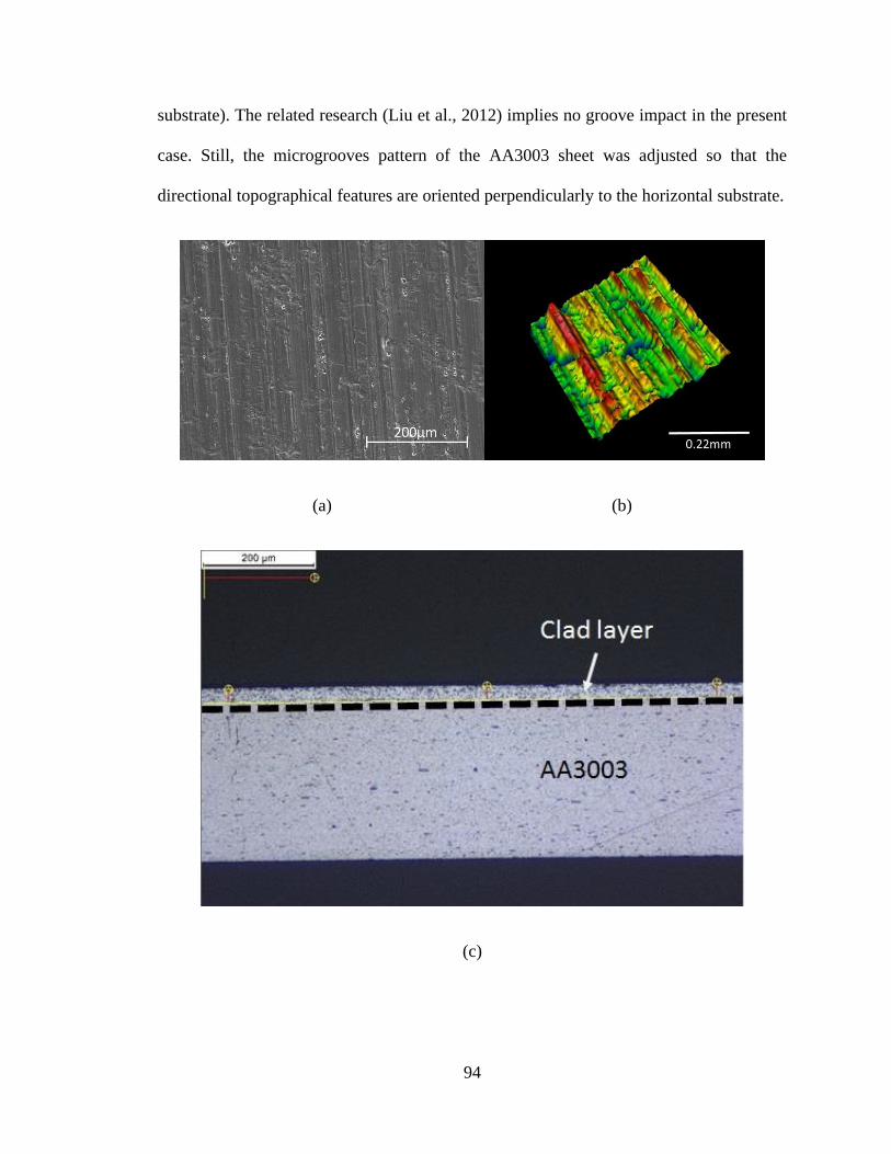
94
substrate). The related research (Liu et al., 2012) implies no groove impact in the present
case. Still, the microgrooves pattern of the AA3003 sheet was adjusted so that the
directional topographical features are oriented perpendicularly to the horizontal substrate.
(a) (b)
(c)
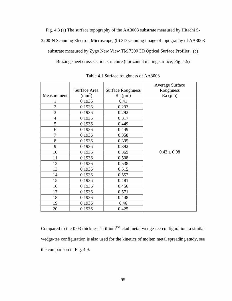
95
Fig. 4.8 (a) The surface topography of the AA3003 substrate measured by Hitachi S-
3200-N Scanning Electron Microscope; (b) 3D scanning image of topography of AA3003
substrate measured by Zygo New View TM 7300 3D Optical Surface Profiler; (c)
Brazing sheet cross section structure (horizontal mating surface, Fig. 4.5)
Table 4.1 Surface roughness of AA3003
Measurement
Surface Area
(mm2)
Surface Roughness
Ra (µm)
Average Surface
Roughness
Ra (µm)
1 0.1936 0.41
2 0.1936 0.293
3 0.1936 0.292
4 0.1936 0.317
5 0.1936 0.449
6 0.1936 0.449
7 0.1936 0.358
8 0.1936 0.395
9 0.1936 0.392
10 0.1936 0.369 0.43 ± 0.08
11 0.1936 0.508
12 0.1936 0.538
13 0.1936 0.515
14 0.1936 0.557
15 0.1936 0.481
16 0.1936 0.456
17 0.1936 0.571
18 0.1936 0.448
19 0.1936 0.46
20 0.1936 0.425
Compared to the 0.03 thickness TrilliumTM clad metal wedge-tee configuration, a similar
wedge-tee configuration is also used for the kinetics of molten metal spreading study, see
the comparison in Fig. 4.9.
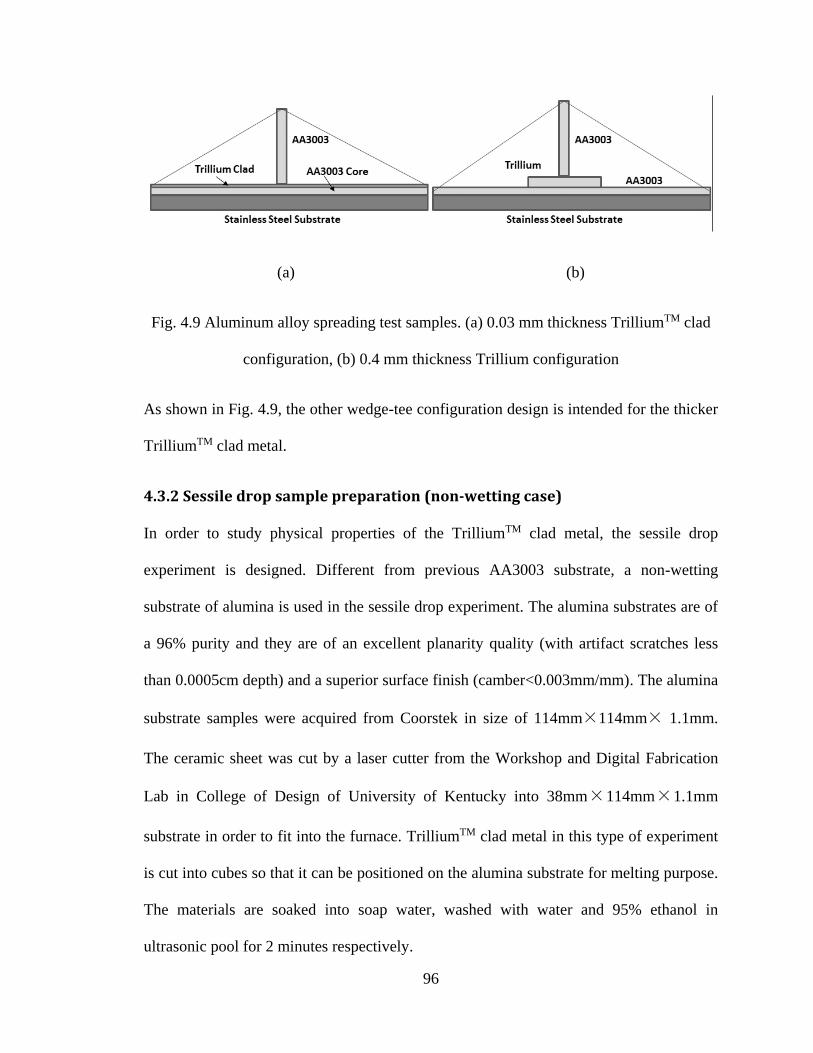
96
(a) (b)
Fig. 4.9 Aluminum alloy spreading test samples. (a) 0.03 mm thickness TrilliumTM clad
configuration, (b) 0.4 mm thickness Trillium configuration
As shown in Fig. 4.9, the other wedge-tee configuration design is intended for the thicker
TrilliumTM clad metal.
4.3.2 Sessile drop sample preparation (non-wetting case)
In order to study physical properties of the TrilliumTM clad metal, the sessile drop
experiment is designed. Different from previous AA3003 substrate, a non-wetting
substrate of alumina is used in the sessile drop experiment. The alumina substrates are of
a 96% purity and they are of an excellent planarity quality (with artifact scratches less
than 0.0005cm depth) and a superior surface finish (camber<0.003mm/mm). The alumina
substrate samples were acquired from Coorstek in size of 114mm×114mm× 1.1mm.
The ceramic sheet was cut by a laser cutter from the Workshop and Digital Fabrication
Lab in College of Design of University of Kentucky into 38mm×114mm×1.1mm
substrate in order to fit into the furnace. TrilliumTM clad metal in this type of experiment
is cut into cubes so that it can be positioned on the alumina substrate for melting purpose.
The materials are soaked into soap water, washed with water and 95% ethanol in
ultrasonic pool for 2 minutes respectively.
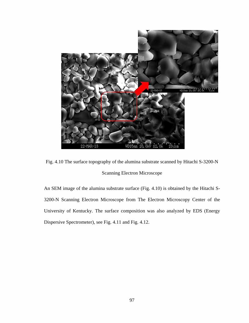
97
Fig. 4.10 The surface topography of the alumina substrate scanned by Hitachi S-3200-N
Scanning Electron Microscope
An SEM image of the alumina substrate surface (Fig. 4.10) is obtained by the Hitachi S-
3200-N Scanning Electron Microscope from The Electron Microscopy Center of the
University of Kentucky. The surface composition was also analyzed by EDS (Energy
Dispersive Spectrometer), see Fig. 4.11 and Fig. 4.12.
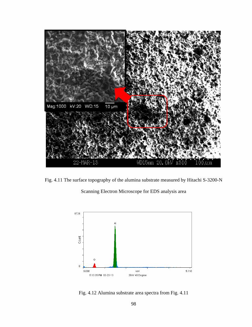
98
Fig. 4.11 The surface topography of the alumina substrate measured by Hitachi S-3200-N
Scanning Electron Microscope for EDS analysis area
Fig. 4.12 Alumina substrate area spectra from Fig. 4.11
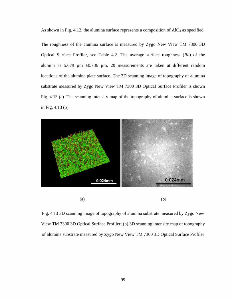
99
As shown in Fig. 4.12, the alumina surface represents a composition of AlO2 as specified.
The roughness of the alumina surface is measured by Zygo New View TM 7300 3D
Optical Surface Profiler, see Table 4.2. The average surface roughness (Ra) of the
alumina is 5.679 µm ±0.736 µm. 20 measurements are taken at different random
locations of the alumina plate surface. The 3D scanning image of topography of alumina
substrate measured by Zygo New View TM 7300 3D Optical Surface Profiler is shown
Fig. 4.13 (a). The scanning intensity map of the topography of alumina surface is shown
in Fig. 4.13 (b).
(a) (b)
Fig. 4.13 3D scanning image of topography of alumina substrate measured by Zygo New
View TM 7300 3D Optical Surface Profiler; (b) 3D scanning intensity map of topography
of alumina substrate measured by Zygo New View TM 7300 3D Optical Surface Profiler
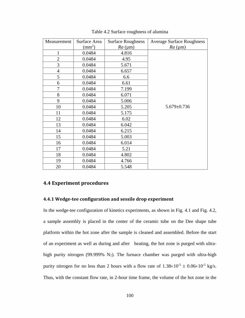
100
Table 4.2 Surface roughness of alumina
Measurement
Surface Area
(mm2)
Surface Roughness
Ra (µm)
Average Surface Roughness
Ra (µm)
1 0.0484 4.816
2 0.0484 4.95
3 0.0484 5.671
4 0.0484 6.657
5 0.0484 6.6
6 0.0484 6.61
7 0.0484 7.199
8 0.0484 6.071
9 0.0484 5.006
10 0.0484 5.205 5.679±0.736
11 0.0484 5.175
12 0.0484 6.02
13 0.0484 6.042
14 0.0484 6.215
15 0.0484 5.003
16 0.0484 6.014
17 0.0484 5.21
18 0.0484 4.802
19 0.0484 4.766
20 0.0484 5.548
4.4 Experiment procedures
4.4.1 Wedge-tee configuration and sessile drop experiment
In the wedge-tee configuration of kinetics experiments, as shown in Fig. 4.1 and Fig. 4.2,
a sample assembly is placed in the center of the ceramic tube on the Dee shape tube
platform within the hot zone after the sample is cleaned and assembled. Before the start
of an experiment as well as during and after heating, the hot zone is purged with ultra-
high purity nitrogen (99.999% N2). The furnace chamber was purged with ultra-high
purity nitrogen for no less than 2 hours with a flow rate of 1.3810-5 0.0610-5 kg/s.
Thus, with the constant flow rate, in 2-hour time frame, the volume of the hot zone in the
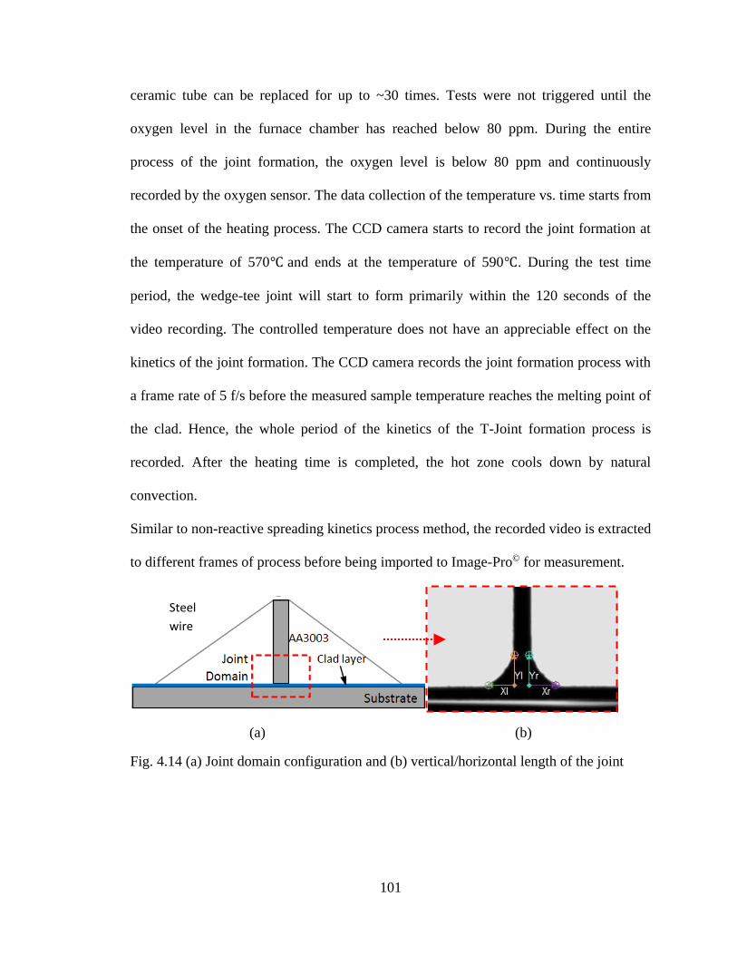
101
ceramic tube can be replaced for up to ~30 times. Tests were not triggered until the
oxygen level in the furnace chamber has reached below 80 ppm. During the entire
process of the joint formation, the oxygen level is below 80 ppm and continuously
recorded by the oxygen sensor. The data collection of the temperature vs. time starts from
the onset of the heating process. The CCD camera starts to record the joint formation at
the temperature of 570℃ and ends at the temperature of 590℃. During the test time
period, the wedge-tee joint will start to form primarily within the 120 seconds of the
video recording. The controlled temperature does not have an appreciable effect on the
kinetics of the joint formation. The CCD camera records the joint formation process with
a frame rate of 5 f/s before the measured sample temperature reaches the melting point of
the clad. Hence, the whole period of the kinetics of the T-Joint formation process is
recorded. After the heating time is completed, the hot zone cools down by natural
convection.
Similar to non-reactive spreading kinetics process method, the recorded video is extracted
to different frames of process before being imported to Image-Pro© for measurement.
(a) (b)
Fig. 4.14 (a) Joint domain configuration and (b) vertical/horizontal length of the joint
Steel
wire
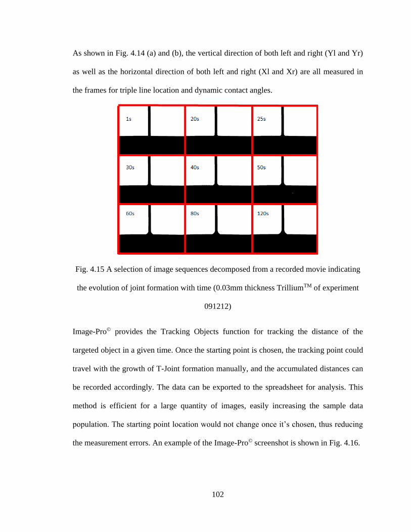
102
As shown in Fig. 4.14 (a) and (b), the vertical direction of both left and right (Yl and Yr)
as well as the horizontal direction of both left and right (Xl and Xr) are all measured in
the frames for triple line location and dynamic contact angles.
Fig. 4.15 A selection of image sequences decomposed from a recorded movie indicating
the evolution of joint formation with time (0.03mm thickness TrilliumTM of experiment
091212)
Image-Pro© provides the Tracking Objects function for tracking the distance of the
targeted object in a given time. Once the starting point is chosen, the tracking point could
travel with the growth of T-Joint formation manually, and the accumulated distances can
be recorded accordingly. The data can be exported to the spreadsheet for analysis. This
method is efficient for a large quantity of images, easily increasing the sample data
population. The starting point location would not change once it’s chosen, thus reducing
the measurement errors. An example of the Image-Pro© screenshot is shown in Fig. 4.16.
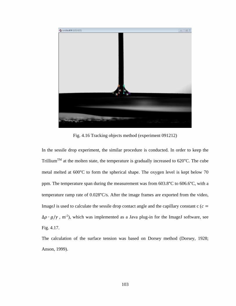
103
Fig. 4.16 Tracking objects method (experiment 091212)
In the sessile drop experiment, the similar procedure is conducted. In order to keep the
TrilliumTM at the molten state, the temperature is gradually increased to 620°C. The cube
metal melted at 600°C to form the spherical shape. The oxygen level is kept below 70
ppm. The temperature span during the measurement was from 603.8°C to 606.6°C, with a
temperature ramp rate of 0.028°C/s. After the image frames are exported from the video,
ImageJ is used to calculate the sessile drop contact angle and the capillary constant c (𝑐 =
∆𝜌 ∙ 𝑔/𝛾 , m-2), which was implemented as a Java plug-in for the ImageJ software, see
Fig. 4.17.
The calculation of the surface tension was based on Dorsey method (Dorsey, 1928;
Anson, 1999).
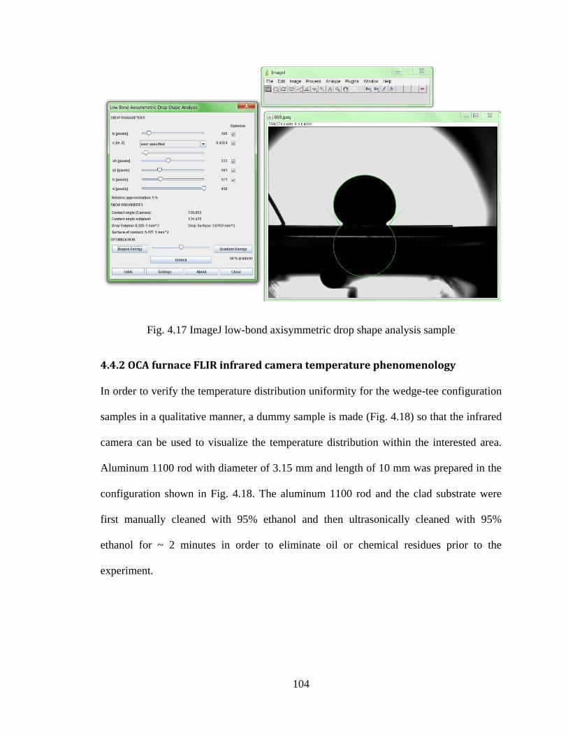
104
Fig. 4.17 ImageJ low-bond axisymmetric drop shape analysis sample
4.4.2 OCA furnace FLIR infrared camera temperature phenomenology
In order to verify the temperature distribution uniformity for the wedge-tee configuration
samples in a qualitative manner, a dummy sample is made (Fig. 4.18) so that the infrared
camera can be used to visualize the temperature distribution within the interested area.
Aluminum 1100 rod with diameter of 3.15 mm and length of 10 mm was prepared in the
configuration shown in Fig. 4.18. The aluminum 1100 rod and the clad substrate were
first manually cleaned with 95% ethanol and then ultrasonically cleaned with 95%
ethanol for ~ 2 minutes in order to eliminate oil or chemical residues prior to the
experiment.
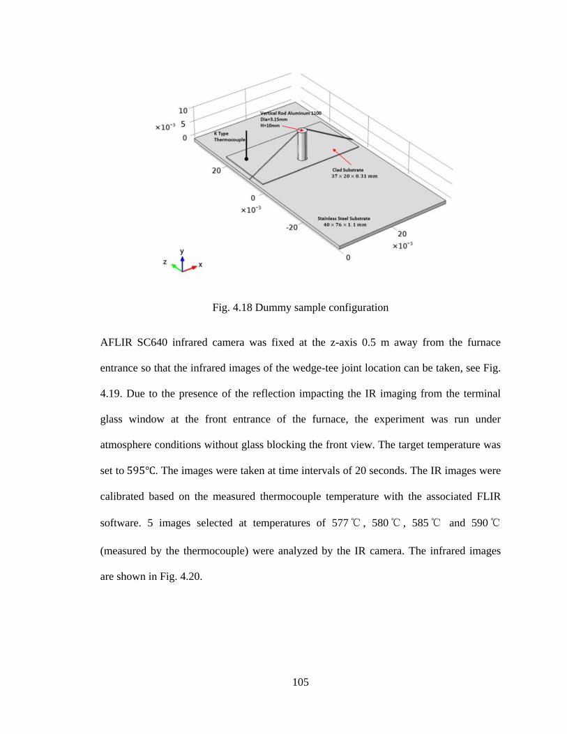
105
Fig. 4.18 Dummy sample configuration
AFLIR SC640 infrared camera was fixed at the z-axis 0.5 m away from the furnace
entrance so that the infrared images of the wedge-tee joint location can be taken, see Fig.
4.19. Due to the presence of the reflection impacting the IR imaging from the terminal
glass window at the front entrance of the furnace, the experiment was run under
atmosphere conditions without glass blocking the front view. The target temperature was
set to 595℃. The images were taken at time intervals of 20 seconds. The IR images were
calibrated based on the measured thermocouple temperature with the associated FLIR
software. 5 images selected at temperatures of 577℃ , 580℃ , 585℃ and 590℃
(measured by the thermocouple) were analyzed by the IR camera. The infrared images
are shown in Fig. 4.20.
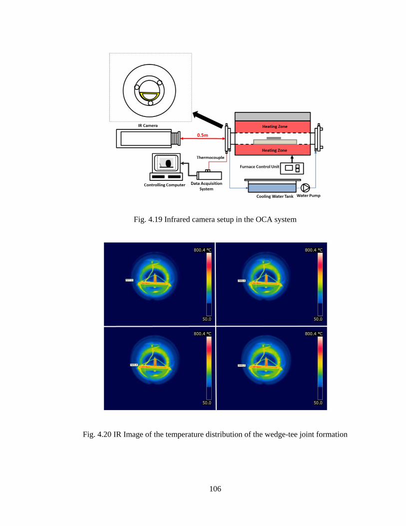
106
Fig. 4.19 Infrared camera setup in the OCA system
Fig. 4.20 IR Image of the temperature distribution of the wedge-tee joint formation
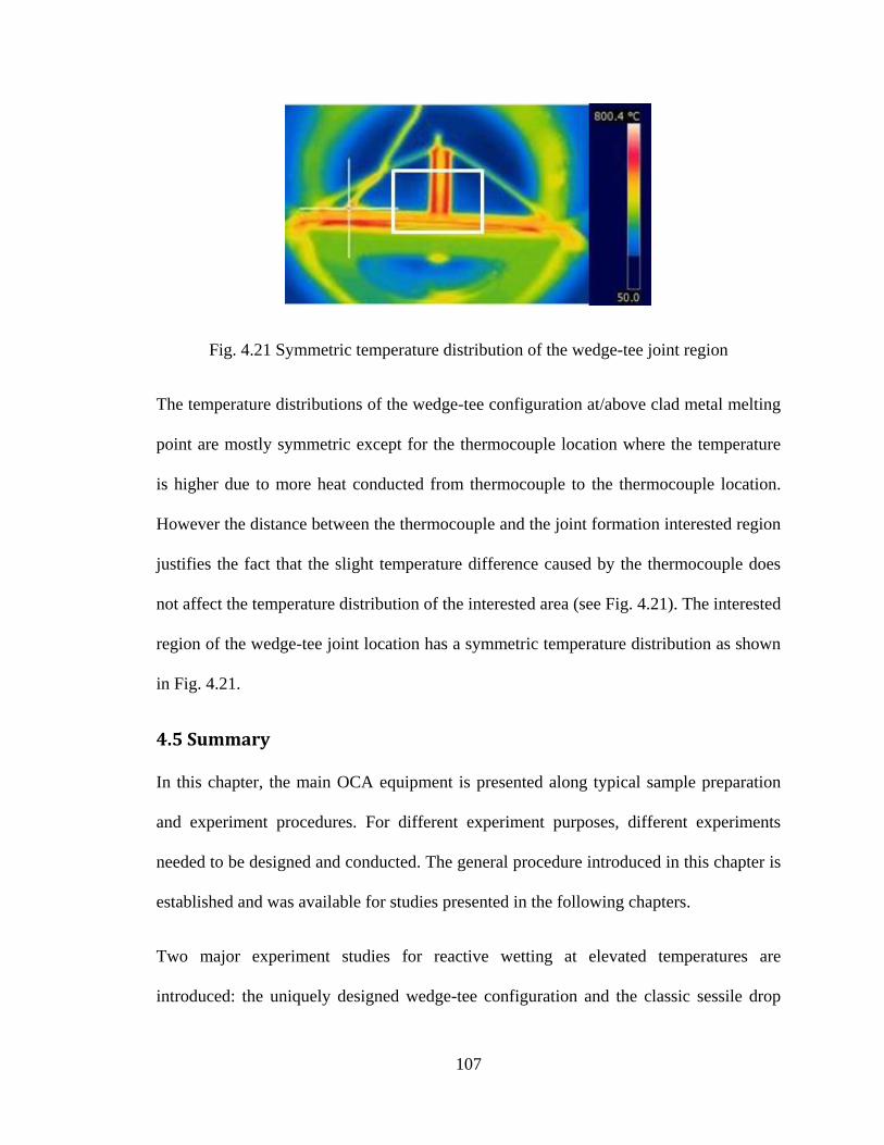
107
Fig. 4.21 Symmetric temperature distribution of the wedge-tee joint region
The temperature distributions of the wedge-tee configuration at/above clad metal melting
point are mostly symmetric except for the thermocouple location where the temperature
is higher due to more heat conducted from thermocouple to the thermocouple location.
However the distance between the thermocouple and the joint formation interested region
justifies the fact that the slight temperature difference caused by the thermocouple does
not affect the temperature distribution of the interested area (see Fig. 4.21). The interested
region of the wedge-tee joint location has a symmetric temperature distribution as shown
in Fig. 4.21.
4.5 Summary
In this chapter, the main OCA equipment is presented along typical sample preparation
and experiment procedures. For different experiment purposes, different experiments
needed to be designed and conducted. The general procedure introduced in this chapter is
established and was available for studies presented in the following chapters.
Two major experiment studies for reactive wetting at elevated temperatures are
introduced: the uniquely designed wedge-tee configuration and the classic sessile drop
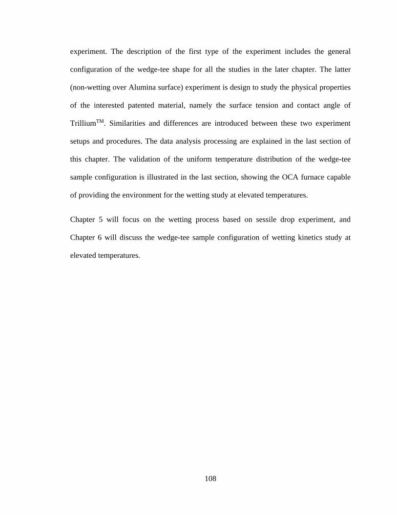
108
experiment. The description of the first type of the experiment includes the general
configuration of the wedge-tee shape for all the studies in the later chapter. The latter
(non-wetting over Alumina surface) experiment is design to study the physical properties
of the interested patented material, namely the surface tension and contact angle of
TrilliumTM. Similarities and differences are introduced between these two experiment
setups and procedures. The data analysis processing are explained in the last section of
this chapter. The validation of the uniform temperature distribution of the wedge-tee
sample configuration is illustrated in the last section, showing the OCA furnace capable
of providing the environment for the wetting study at elevated temperatures.
Chapter 5 will focus on the wetting process based on sessile drop experiment, and
Chapter 6 will discuss the wedge-tee sample configuration of wetting kinetics study at
elevated temperatures.
109
CHAPTER 5: WETTING OF MOLTEN CLAD METAL ON
WETTED AND NON-WETTED SURFACES
5.1 Overview
This chapter mainly focuses on the experimental study of the molten clad metal, namely
TrilliumTM wetting on either wetting surface or the non-wetting surface.
Phenomenological observation, data analysis and the reviewed literature validation will
be discussed here. As the general experiment facility, preparation and procedures have
been introduced in the previous chapter, only specific difference of the experiment
preparation and procedure will be commented on in this chapter.
The wetting of molten TrilliumTM on wetting surface and non-wetting surface was studied
with the Optical Contact Angle Analyzer (OCA), see Chapter 4 for details. The sessile
drop experiment configuration was adopted to study the physical properties of the molten
clad metal at elevated temperatures needed for modeling in latter stages of this project
work (see Appendix E). In the wetting surface case, the substrate used is the same
material (AA3003) that will be used in studies in the following chapter. Thus studying
the simple sessile drop spreading on the wetting surface gives the preliminary insight into
the physical characteristics of the molten clad metal at elevated temperatures. In the non-
wetting surface case, alumina substrate was used in the sessile drop experiment
configuration for the molten clad metal to form the spherical liquid metal shape to
facilitate measuring the unknown surface tension as well as its contact angle based on the
low-bond axisymmetric drop shape analysis (LBADSA) (Stalder et al., 2010). Note that
the molten metal considered represents a novel alloy (composite) and literature data for
surface tension were considered a priori non reliable for this case. The molten sample
110
cross section images were analyzed by SEM and EDS to confirm the eventual liquid
penetration and dissolution of the substrate (existing in the wetting case), and more
complicated de-oxidation, chemical reaction and inter-diffusion phenomena shown in the
non-wetting case. The measured value of surface tension for the new material (namely
TrilliumTM) was validated by comparing evaluated surface tension data to the known
experiment values from multiple different literature sources of similar metal alloy
systems.
5.2 Experimental study of the molten clad metal at elevated
temperatures
As mentioned earlier, the sessile drop configuration was adopted to study the
phenomenological analysis of the molten clad metal wetting process. The prepared
samples were placed on the Dee shape tubing, so that the heating chamber can be purged
with ultra-high purity nitrogen (99.999% N2) for more than 2 hours with a flow rate of
1.3810-5 0.0610-5 kg/s. Tests were not triggered until the oxygen level in the
furnace chamber has reached below 60 – 80 ppm. The CCD camera starts to record when
the clad metal TrilliumTM is melting at its melting temperature of 580 ± 5℃. The frame
rate of the recoding CCD camera was 25 frames/s. The recorded video was extracted into
Image-Pro© as well as ImageJ for measurement of surface tension and contact angle.
5.2.1 Molten clad metal wetting on the wetting surface – preliminary tests
To ensure the equilibrium state of the liquid clad metal under nearly isothermal state at
the peak temperature, the molten metal, formed from a solid alloy sample, initially cut
into a 0.1979 g cube, was positioned on the AA3003 substrate. The run lasted
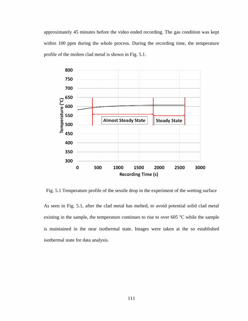
111
approximately 45 minutes before the video ended recording. The gas condition was kept
within 100 ppm during the whole process. During the recording time, the temperature
profile of the molten clad metal is shown in Fig. 5.1.
Fig. 5.1 Temperature profile of the sessile drop in the experiment of the wetting surface
As seen in Fig. 5.1, after the clad metal has melted, to avoid potential solid clad metal
existing in the sample, the temperature continues to rise to over 605 °C while the sample
is maintained in the near isothermal state. Images were taken at the so established
isothermal state for data analysis.
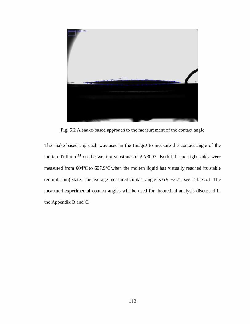
112
Fig. 5.2 A snake-based approach to the measurement of the contact angle
The snake-based approach was used in the ImageJ to measure the contact angle of the
molten TrilliumTM on the wetting substrate of AA3003. Both left and right sides were
measured from 604℃ to 607.9℃ when the molten liquid has virtually reached its stable
(equilibrium) state. The average measured contact angle is 6.9°±2.7°, see Table 5.1. The
measured experimental contact angles will be used for theoretical analysis discussed in
the Appendix B and C.
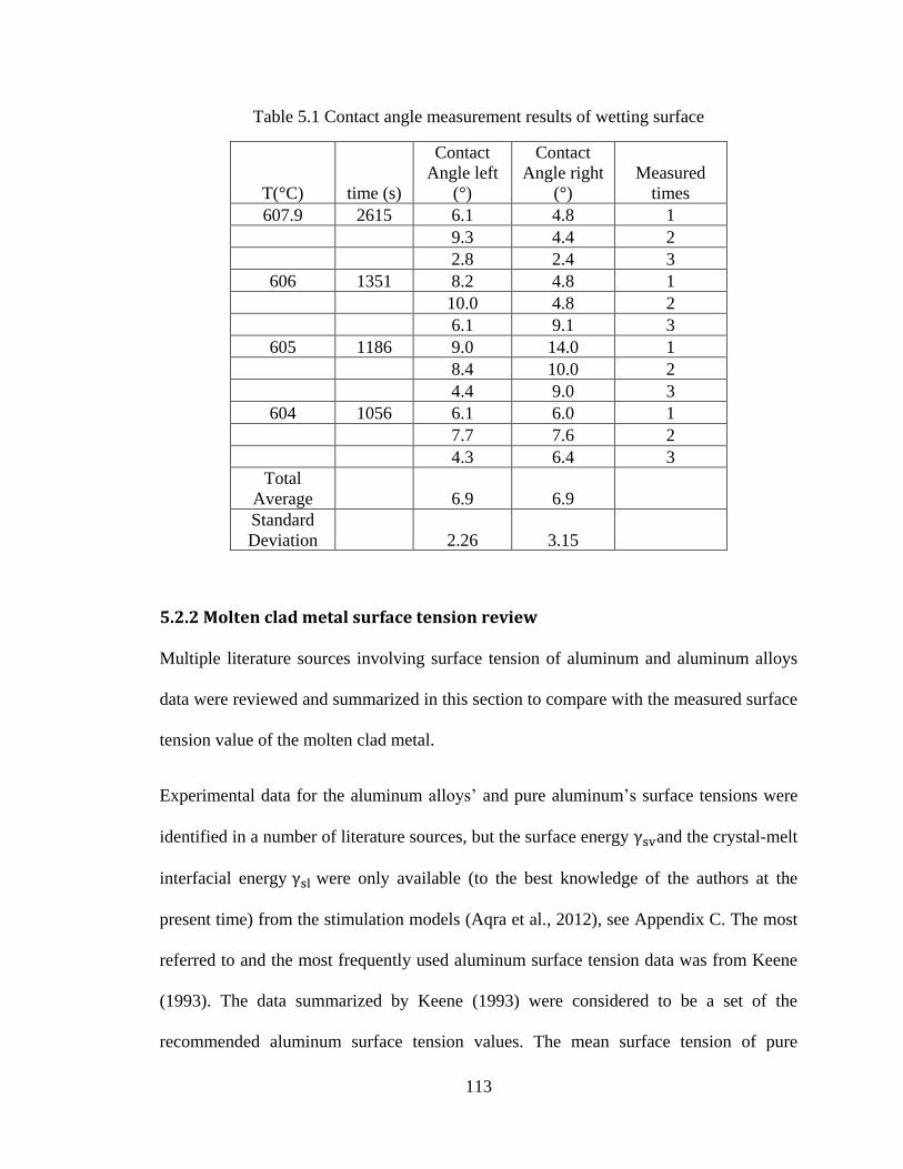
113
Table 5.1 Contact angle measurement results of wetting surface
T(°C) time (s)
Contact
Angle left
(°)
Contact
Angle right
(°)
Measured
times
607.9 2615 6.1 4.8 1
9.3 4.4 2
2.8 2.4 3
606 1351 8.2 4.8 1
10.0 4.8 2
6.1 9.1 3
605 1186 9.0 14.0 1
8.4 10.0 2
4.4 9.0 3
604 1056 6.1 6.0 1
7.7 7.6 2
4.3 6.4 3
Total
Average 6.9 6.9
Standard
Deviation 2.26 3.15
5.2.2 Molten clad metal surface tension review
Multiple literature sources involving surface tension of aluminum and aluminum alloys
data were reviewed and summarized in this section to compare with the measured surface
tension value of the molten clad metal.
Experimental data for the aluminum alloys’ and pure aluminum’s surface tensions were
identified in a number of literature sources, but the surface energy γsvand the crystal-melt
interfacial energy γsl were only available (to the best knowledge of the authors at the
present time) from the stimulation models (Aqra et al., 2012), see Appendix C. The most
referred to and the most frequently used aluminum surface tension data was from Keene
(1993). The data summarized by Keene (1993) were considered to be a set of the
recommended aluminum surface tension values. The mean surface tension of pure
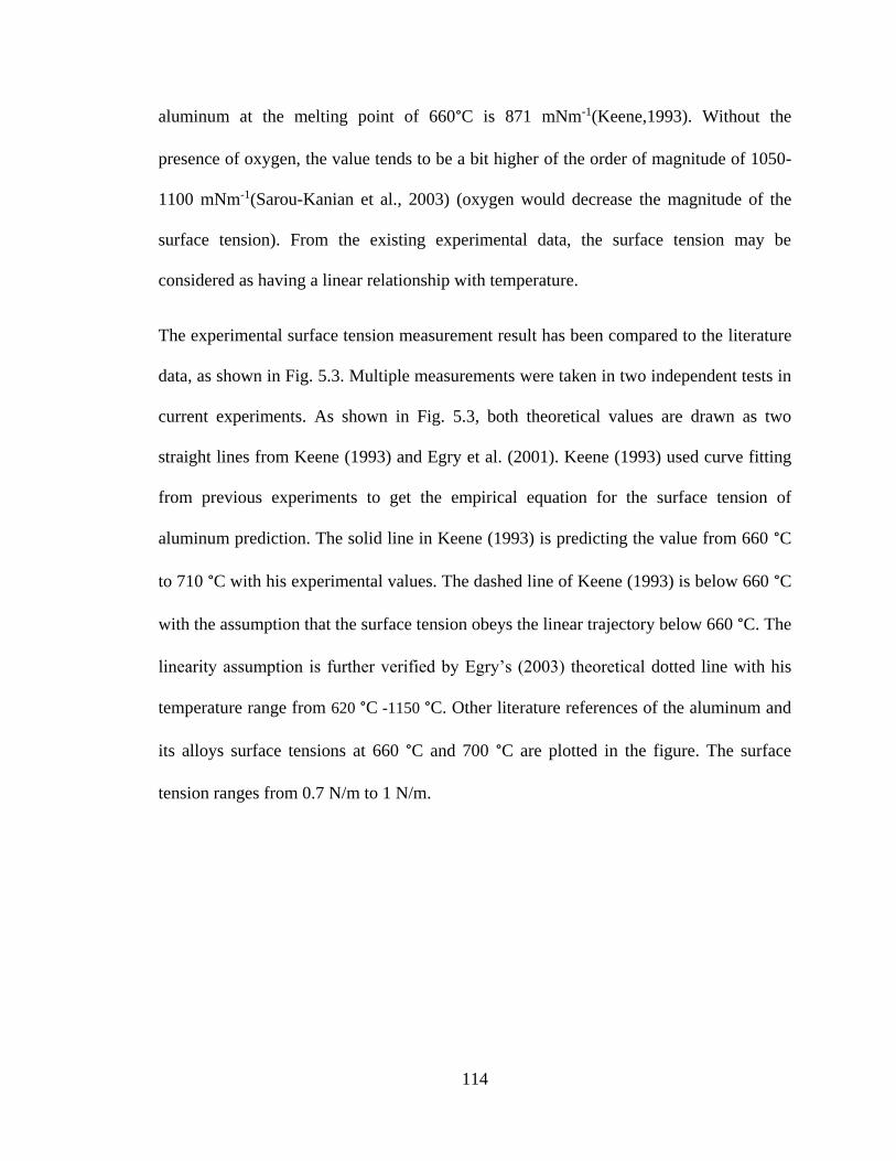
114
aluminum at the melting point of 660°C is 871 mNm-1(Keene,1993). Without the
presence of oxygen, the value tends to be a bit higher of the order of magnitude of 1050-
1100 mNm-1(Sarou-Kanian et al., 2003) (oxygen would decrease the magnitude of the
surface tension). From the existing experimental data, the surface tension may be
considered as having a linear relationship with temperature.
The experimental surface tension measurement result has been compared to the literature
data, as shown in Fig. 5.3. Multiple measurements were taken in two independent tests in
current experiments. As shown in Fig. 5.3, both theoretical values are drawn as two
straight lines from Keene (1993) and Egry et al. (2001). Keene (1993) used curve fitting
from previous experiments to get the empirical equation for the surface tension of
aluminum prediction. The solid line in Keene (1993) is predicting the value from 660 °C
to 710 °C with his experimental values. The dashed line of Keene (1993) is below 660 °C
with the assumption that the surface tension obeys the linear trajectory below 660 °C. The
linearity assumption is further verified by Egry’s (2003) theoretical dotted line with his
temperature range from 620 °C -1150 °C. Other literature references of the aluminum and
its alloys surface tensions at 660 °C and 700 °C are plotted in the figure. The surface
tension ranges from 0.7 N/m to 1 N/m.
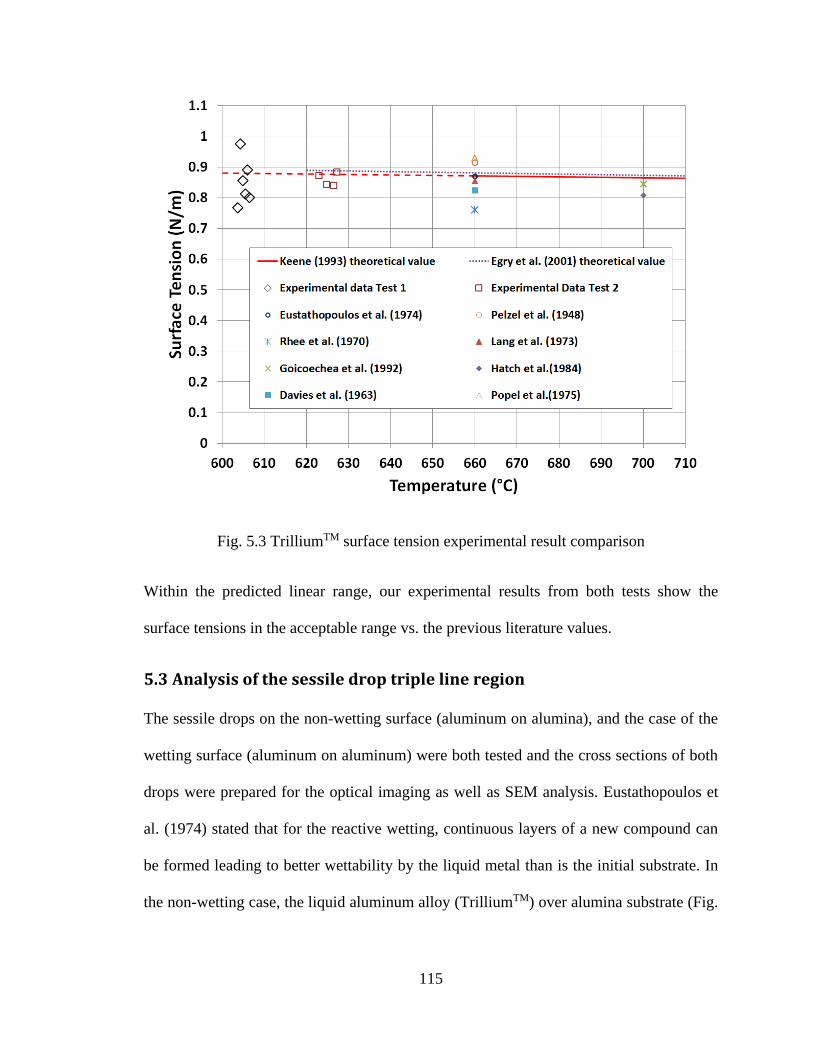
115
Fig. 5.3 TrilliumTM surface tension experimental result comparison
Within the predicted linear range, our experimental results from both tests show the
surface tensions in the acceptable range vs. the previous literature values.
5.3 Analysis of the sessile drop triple line region
The sessile drops on the non-wetting surface (aluminum on alumina), and the case of the
wetting surface (aluminum on aluminum) were both tested and the cross sections of both
drops were prepared for the optical imaging as well as SEM analysis. Eustathopoulos et
al. (1974) stated that for the reactive wetting, continuous layers of a new compound can
be formed leading to better wettability by the liquid metal than is the initial substrate. In
the non-wetting case, the liquid aluminum alloy (TrilliumTM) over alumina substrate (Fig.
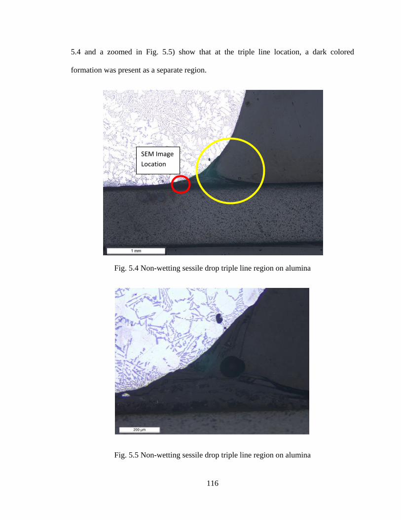
116
5.4 and a zoomed in Fig. 5.5) show that at the triple line location, a dark colored
formation was present as a separate region.
Fig. 5.4 Non-wetting sessile drop triple line region on alumina
Fig. 5.5 Non-wetting sessile drop triple line region on alumina
SEM Image
Location
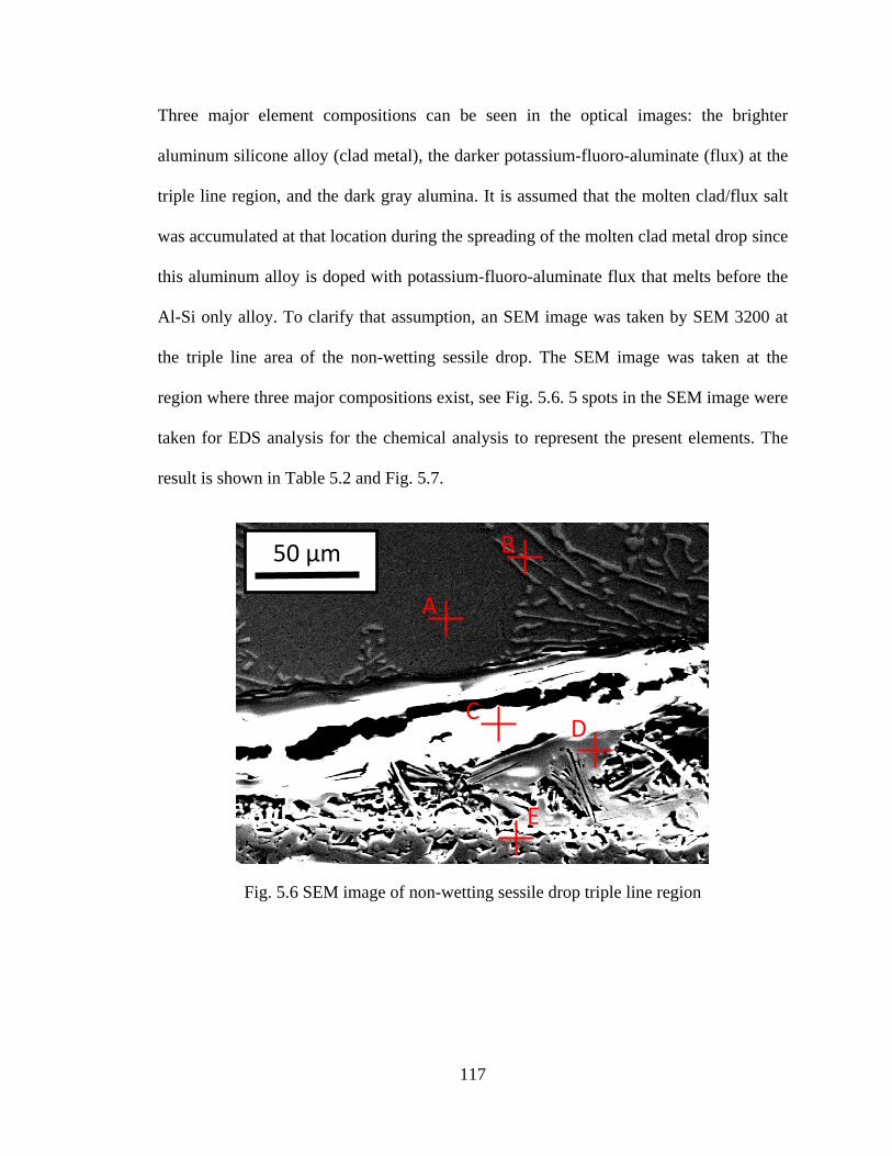
117
Three major element compositions can be seen in the optical images: the brighter
aluminum silicone alloy (clad metal), the darker potassium-fluoro-aluminate (flux) at the
triple line region, and the dark gray alumina. It is assumed that the molten clad/flux salt
was accumulated at that location during the spreading of the molten clad metal drop since
this aluminum alloy is doped with potassium-fluoro-aluminate flux that melts before the
Al-Si only alloy. To clarify that assumption, an SEM image was taken by SEM 3200 at
the triple line area of the non-wetting sessile drop. The SEM image was taken at the
region where three major compositions exist, see Fig. 5.6. 5 spots in the SEM image were
taken for EDS analysis for the chemical analysis to represent the present elements. The
result is shown in Table 5.2 and Fig. 5.7.
Fig. 5.6 SEM image of non-wetting sessile drop triple line region
50 µm
A
B
C D
E
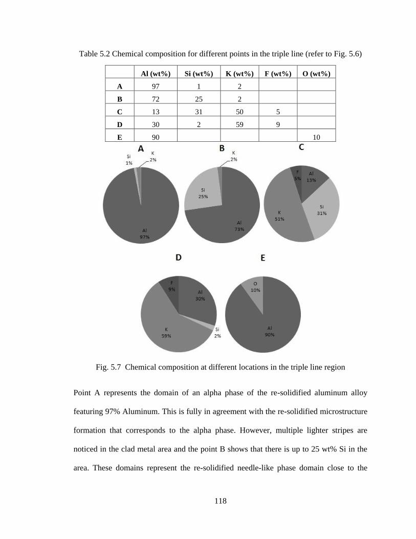
118
Table 5.2 Chemical composition for different points in the triple line (refer to Fig. 5.6)
Al (wt%) Si (wt%) K (wt%) F (wt%) O (wt%)
A 97 1 2
B 72 25 2
C 13 31 50 5
D 30 2 59 9
E 90
10
Fig. 5.7 Chemical composition at different locations in the triple line region
Point A represents the domain of an alpha phase of the re-solidified aluminum alloy
featuring 97% Aluminum. This is fully in agreement with the re-solidified microstructure
formation that corresponds to the alpha phase. However, multiple lighter stripes are
noticed in the clad metal area and the point B shows that there is up to 25 wt% Si in the
area. These domains represent the re-solidified needle-like phase domain close to the
119
eutectic or, more precisely above the eutectic composition. The white phase area, C,
features a rich potassium domain of 51% of K, with the lowest Al content (13%) and the
highest Si content (31%). Yet another domain, point D features the highest potassium
level of 59 wt%. The surface of alumina as represented by point E shows that the
composition for the alumina surface didn't change during the spreading or the re-
solidification process of the molten clad metal drop. The porous configuration of the
alumina surface shown in Fig. 5.6 has verified the roughness of the surface configuration.
As assumed, the result verifies that the first dark region is composed of aluminum-
silicone alloy with minor potassium. The middle region where the triple line region is
positioned (both C and D) features a large amount of potassium which corresponds to the
potassium-fluoro-aluminate flux. The bottom region is proven to be alumina shown as E
in the table, see Fig. 5.6.
Based on the EDS result, it can be stated that during the spreading of the sessile drop (due
to the lower melting point of the brazing flux of potassium fluoride, as well as silicon
contained in the clad metal), a layer of liquid flux is formed on the surface of the liquid
molten clad metal preventing oxidation. A large amount of the flux accumulates at the
triple line region. It is speculated that the molten clad metal spreads primarily across the
exposed alumina surface, and in the process squeezes the liquid accumulation of the flux
in the triple line area, forming complex multilayered phases observed in Fig. 5.6.
In the wetting case, the triple line region is relatively simple (based on the images taken
by the optical camera, see Fig. 5.8 and Fig. 5.9). The clear alpha phase aluminum and
eutectic phase can be observed at the intersection area between the TrilliumTM and the
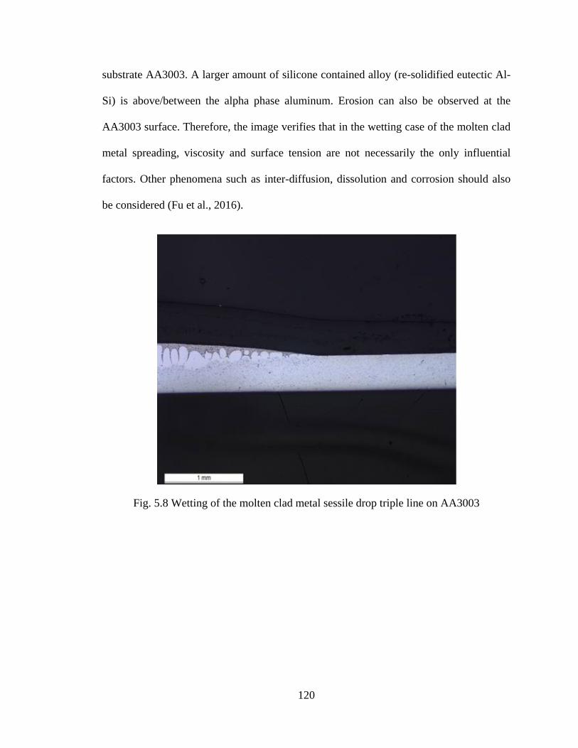
120
substrate AA3003. A larger amount of silicone contained alloy (re-solidified eutectic Al-
Si) is above/between the alpha phase aluminum. Erosion can also be observed at the
AA3003 surface. Therefore, the image verifies that in the wetting case of the molten clad
metal spreading, viscosity and surface tension are not necessarily the only influential
factors. Other phenomena such as inter-diffusion, dissolution and corrosion should also
be considered (Fu et al., 2016).
Fig. 5.8 Wetting of the molten clad metal sessile drop triple line on AA3003
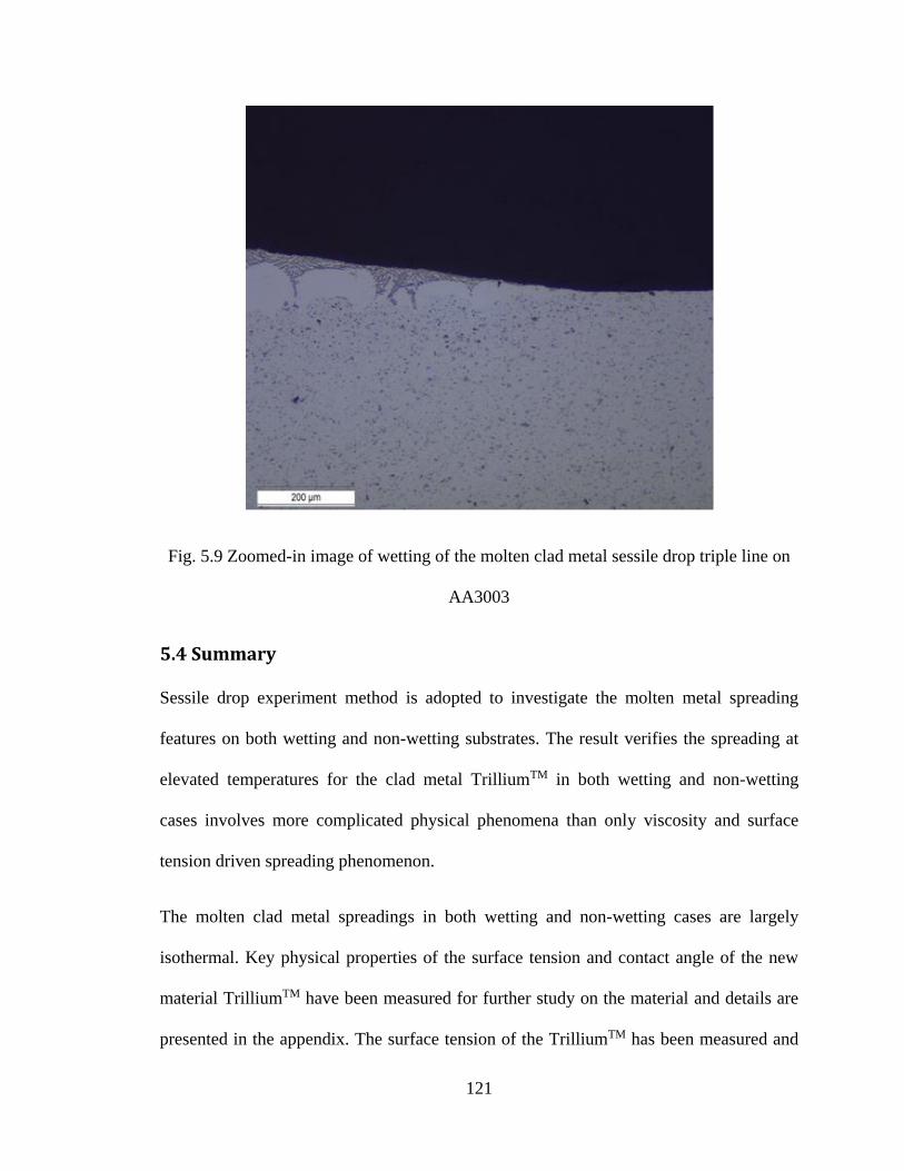
121
Fig. 5.9 Zoomed-in image of wetting of the molten clad metal sessile drop triple line on
AA3003
5.4 Summary
Sessile drop experiment method is adopted to investigate the molten metal spreading
features on both wetting and non-wetting substrates. The result verifies the spreading at
elevated temperatures for the clad metal TrilliumTM in both wetting and non-wetting
cases involves more complicated physical phenomena than only viscosity and surface
tension driven spreading phenomenon.
The molten clad metal spreadings in both wetting and non-wetting cases are largely
isothermal. Key physical properties of the surface tension and contact angle of the new
material TrilliumTM have been measured for further study on the material and details are
presented in the appendix. The surface tension of the TrilliumTM has been measured and
122
compared to multiple references (see Appendix). Based on the theoretical predictions
from both Keene (1993) and Egry et al. (2001), the measured surface tension falls in the
expected range of aluminum alloy surface tension. The measured surface tension of the
new flux-less aluminum alloy serves a critical role in the study.
The triple line region of the sessile drop on the non-wetting and wetting substrates are
further analyzed after its re-solidification. In the non-wetting case, the triple line regime
presents a more complicated phenomenon. The molten flux, the potassium-fluoro-
aluminate contained in the clad metal forms a layer on top of the molten clad metal
preventing metal beneath from oxidation. However, flux accumulated at the triple line
region forms a ridge. Other phenomena, such as inter-diffusion and erosion can also be
observed in the non-wetting spreading of the clad metal. In the wetting case, based on the
optical image of the molten metal on AA3003 after re-solidification, the alpha phase
aluminum can be seen at the intersection between TrilliumTM and AA3003 and the
silicone rich eutectic phase separates at the top of the drop. During the spreading process,
surface tension and viscosity are no longer the dominating forces in this region, hence
more complicated phenomena such as inter-diffusion and erosion and liquid penetration
can clearly be seen in those images.
.
123
CHAPTER 6: WEDGE-TEE CONFIGURATION KINETICS OF
THE CAPILLARY FLOW OF MOLTEN CLAD
6.1 Overview
This chapter discusses the experimental study of a specific configuration of mating
surfaces (a wedge-tee). The near reactive wetting kinetics at elevated temperatures is
considered. The specific configuration is similar to the Wilhelmy plate configuration in
the non-reactive wetting studies reported above. In the current configuration, both
vertical and horizontal plates are fixed to each other before brazing without any
movement. This simulates the joint area formed by the extended surfaces on substrates
like the fins in heat exchangers. The sample preparation is introduced in Chapter 4. While
Chapter 3 addresses the similar configuration for a non-reactive spreading, serving as the
benchmark reference.
Different clad metal forms were investigated in the wedge-tee configuration by changing
the clad metal layer thickness. The 2-D configurations of the observed clad metal liquid
joint zone formation at elevated temperatures during a time evolution of the molten metal
free surface spreading are captured via the Optical Contact Angle Analyzer (OCA)
system. It is found that the triple line kinetics features a sequence of multiple spreading
phases. These phases of the joint formation are identified and the influential parameters
are assessed (Fu et al., 2013). An empirical power law relationship based on the kinetics
of the triple line is established for different configurations of the wedge-tee joints.
Different clad metal layer thickness and the substrate surface wetting properties, lead to
different equilibrium height of the triple line location. It can be observed, due to a change
124
in the availability of the molten clad metal at the joint location, that liquid rise greatly
depends on an availability of liquid in the pool if the quantity of liquid becomes smaller
than some pre-defined quantity related to the total volume of liquid in the joint, formed
with an unrestricted flow up to the equilibrium location of the triple line.. The final result
of the wedge-tee joint formation kinetics has been compared to the benchmark tests
investigated in previous chapters. Numerical analysis also confirms the experimental
procedures as well as the experimental results. It can be concluded that in the wedge-tee
configuration spreading at elevated temperatures, surface tension and viscosity are not the
only controlling factors. Physical phenomena such as inter-diffusion, erosion and liquid
metal penetration along the grain boundaries are all taking place at the same time during
the process evolution.
6.2 Experimental study of the molten clad metal spreading kinetics in a
wedge-tee configuration at elevated temperatures
6.2.1 Molten clad metal kinetics study methodology
The wedge-tee sample preparation and experimental procedure have been introduced in
Chapter 4. Three clad metal layer thicknesses have been investigated in the wedge-tee
joint configuration. These include, 0.03mm, 0.4mm and 0.8mm thickness of clad metal
TrilliumTM, see Fig. 6.1. In these configurations, the vertical plate AA3003 has
dimensions of 10×10×0.4 mm (in a, b and c configurations), TrilliumTM clad metal sheet
(horizontal) has dimensions of 10×37×0.32 mm with 0.03 mm thickness TrilliumTM clad
on the top (configuration a), the AA3003 substrate is 10×37×0.4 mm and the Trillium
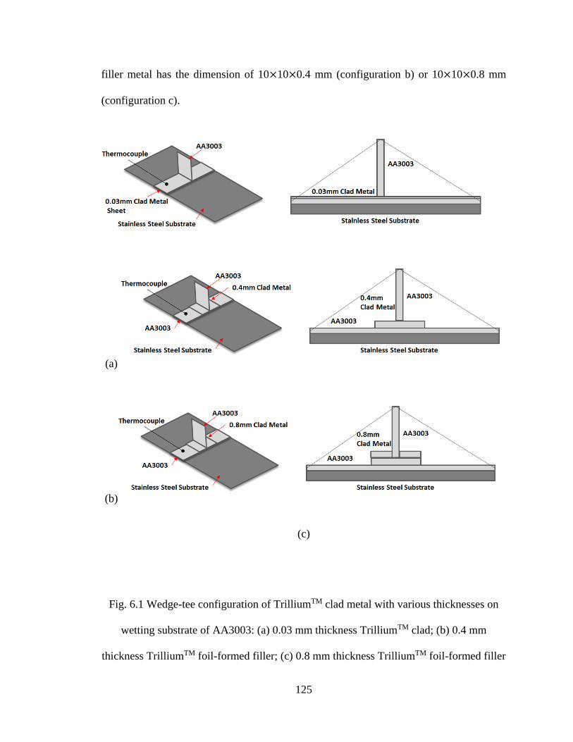
125
filler metal has the dimension of 10×10×0.4 mm (configuration b) or 10×10×0.8 mm
(configuration c).
(a)
(b)
(c)
Fig. 6.1 Wedge-tee configuration of TrilliumTM clad metal with various thicknesses on
wetting substrate of AA3003: (a) 0.03 mm thickness TrilliumTM clad; (b) 0.4 mm
thickness TrilliumTM foil-formed filler; (c) 0.8 mm thickness TrilliumTM foil-formed filler
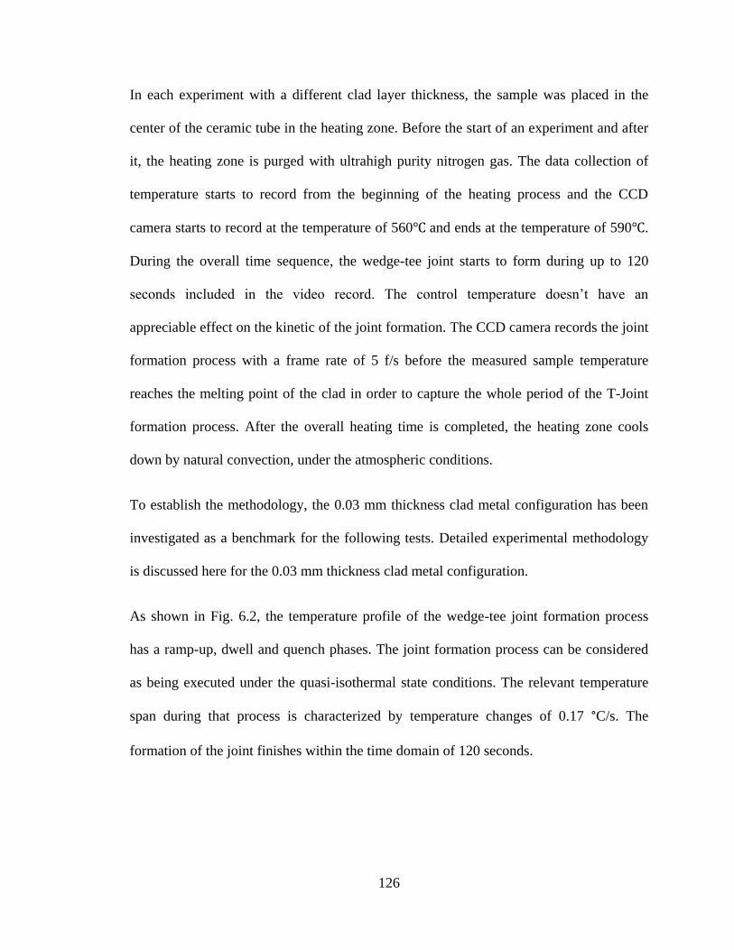
126
In each experiment with a different clad layer thickness, the sample was placed in the
center of the ceramic tube in the heating zone. Before the start of an experiment and after
it, the heating zone is purged with ultrahigh purity nitrogen gas. The data collection of
temperature starts to record from the beginning of the heating process and the CCD
camera starts to record at the temperature of 560℃ and ends at the temperature of 590℃.
During the overall time sequence, the wedge-tee joint starts to form during up to 120
seconds included in the video record. The control temperature doesn’t have an
appreciable effect on the kinetic of the joint formation. The CCD camera records the joint
formation process with a frame rate of 5 f/s before the measured sample temperature
reaches the melting point of the clad in order to capture the whole period of the T-Joint
formation process. After the overall heating time is completed, the heating zone cools
down by natural convection, under the atmospheric conditions.
To establish the methodology, the 0.03 mm thickness clad metal configuration has been
investigated as a benchmark for the following tests. Detailed experimental methodology
is discussed here for the 0.03 mm thickness clad metal configuration.
As shown in Fig. 6.2, the temperature profile of the wedge-tee joint formation process
has a ramp-up, dwell and quench phases. The joint formation process can be considered
as being executed under the quasi-isothermal state conditions. The relevant temperature
span during that process is characterized by temperature changes of 0.17 °C/s. The
formation of the joint finishes within the time domain of 120 seconds.
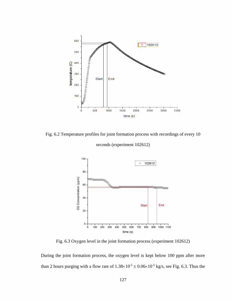
127
Fig. 6.2 Temperature profiles for joint formation process with recordings of every 10
seconds (experiment 102612)
Fig. 6.3 Oxygen level in the joint formation process (experiment 102612)
During the joint formation process, the oxygen level is kept below 100 ppm after more
than 2 hours purging with a flow rate of 1.3810-5 0.0610-5 kg/s, see Fig. 6.3. Thus the
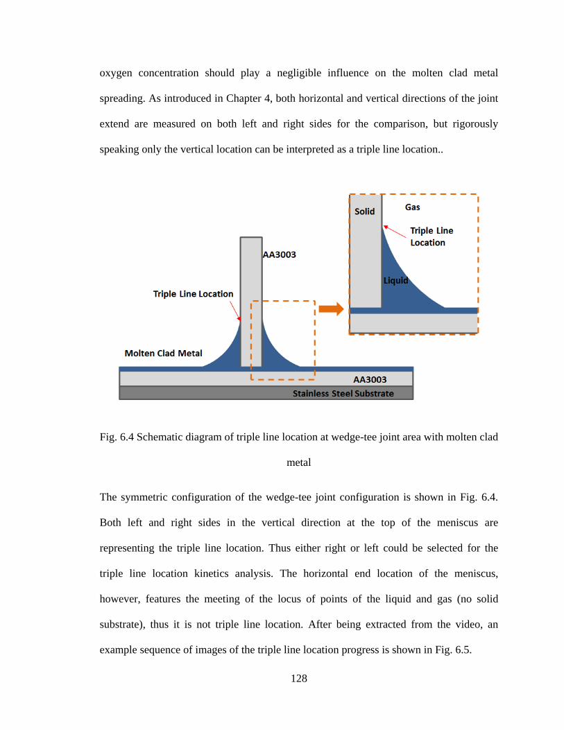
128
oxygen concentration should play a negligible influence on the molten clad metal
spreading. As introduced in Chapter 4, both horizontal and vertical directions of the joint
extend are measured on both left and right sides for the comparison, but rigorously
speaking only the vertical location can be interpreted as a triple line location..
Fig. 6.4 Schematic diagram of triple line location at wedge-tee joint area with molten clad
metal
The symmetric configuration of the wedge-tee joint configuration is shown in Fig. 6.4.
Both left and right sides in the vertical direction at the top of the meniscus are
representing the triple line location. Thus either right or left could be selected for the
triple line location kinetics analysis. The horizontal end location of the meniscus,
however, features the meeting of the locus of points of the liquid and gas (no solid
substrate), thus it is not triple line location. After being extracted from the video, an
example sequence of images of the triple line location progress is shown in Fig. 6.5.
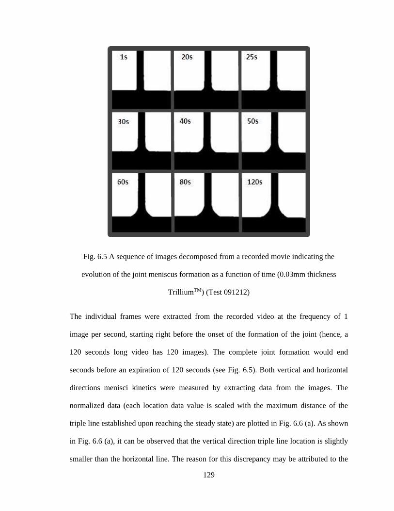
129
Fig. 6.5 A sequence of images decomposed from a recorded movie indicating the
evolution of the joint meniscus formation as a function of time (0.03mm thickness
TrilliumTM) (Test 091212)
The individual frames were extracted from the recorded video at the frequency of 1
image per second, starting right before the onset of the formation of the joint (hence, a
120 seconds long video has 120 images). The complete joint formation would end
seconds before an expiration of 120 seconds (see Fig. 6.5). Both vertical and horizontal
directions menisci kinetics were measured by extracting data from the images. The
normalized data (each location data value is scaled with the maximum distance of the
triple line established upon reaching the steady state) are plotted in Fig. 6.6 (a). As shown
in Fig. 6.6 (a), it can be observed that the vertical direction triple line location is slightly
smaller than the horizontal line. The reason for this discrepancy may be attributed to the
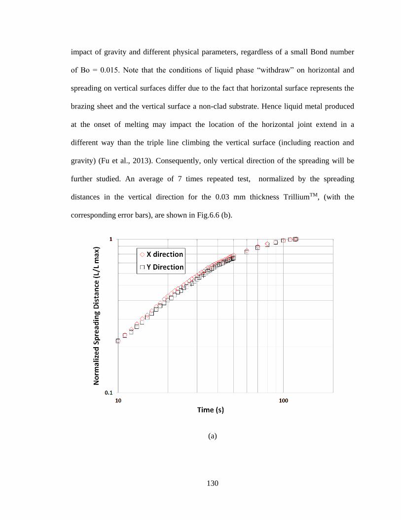
130
impact of gravity and different physical parameters, regardless of a small Bond number
of Bo = 0.015. Note that the conditions of liquid phase “withdraw” on horizontal and
spreading on vertical surfaces differ due to the fact that horizontal surface represents the
brazing sheet and the vertical surface a non-clad substrate. Hence liquid metal produced
at the onset of melting may impact the location of the horizontal joint extend in a
different way than the triple line climbing the vertical surface (including reaction and
gravity) (Fu et al., 2013). Consequently, only vertical direction of the spreading will be
further studied. An average of 7 times repeated test, normalized by the spreading
distances in the vertical direction for the 0.03 mm thickness TrilliumTM, (with the
corresponding error bars), are shown in Fig.6.6 (b).
(a)
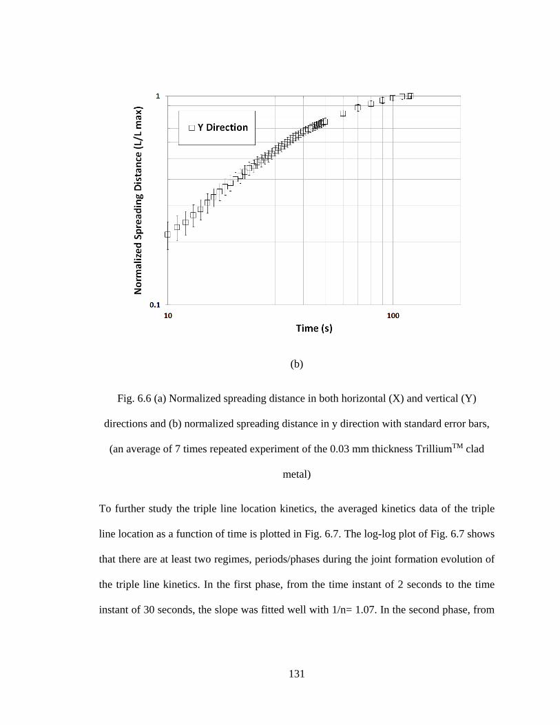
131
(b)
Fig. 6.6 (a) Normalized spreading distance in both horizontal (X) and vertical (Y)
directions and (b) normalized spreading distance in y direction with standard error bars,
(an average of 7 times repeated experiment of the 0.03 mm thickness TrilliumTM clad
metal)
To further study the triple line location kinetics, the averaged kinetics data of the triple
line location as a function of time is plotted in Fig. 6.7. The log-log plot of Fig. 6.7 shows
that there are at least two regimes, periods/phases during the joint formation evolution of
the triple line kinetics. In the first phase, from the time instant of 2 seconds to the time
instant of 30 seconds, the slope was fitted well with 1/n= 1.07. In the second phase, from
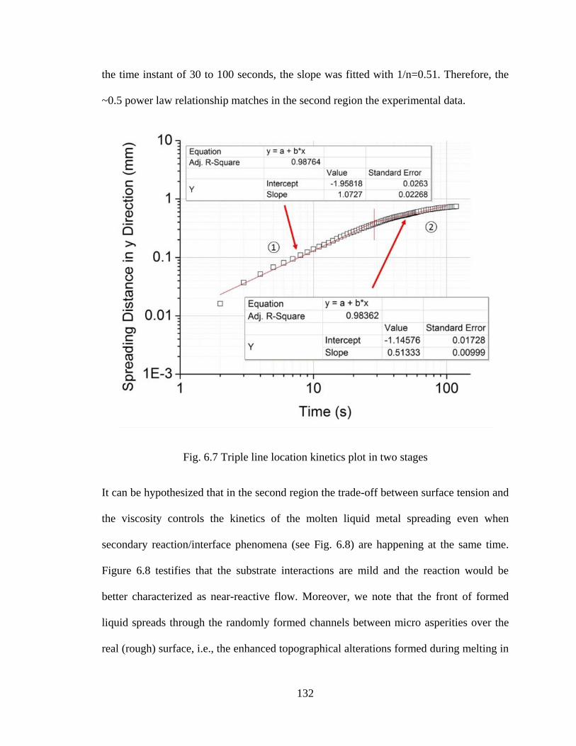
132
the time instant of 30 to 100 seconds, the slope was fitted with 1/n=0.51. Therefore, the
~0.5 power law relationship matches in the second region the experimental data.
Fig. 6.7 Triple line location kinetics plot in two stages
It can be hypothesized that in the second region the trade-off between surface tension and
the viscosity controls the kinetics of the molten liquid metal spreading even when
secondary reaction/interface phenomena (see Fig. 6.8) are happening at the same time.
Figure 6.8 testifies that the substrate interactions are mild and the reaction would be
better characterized as near-reactive flow. Moreover, we note that the front of formed
liquid spreads through the randomly formed channels between micro asperities over the
real (rough) surface, i.e., the enhanced topographical alterations formed during melting in
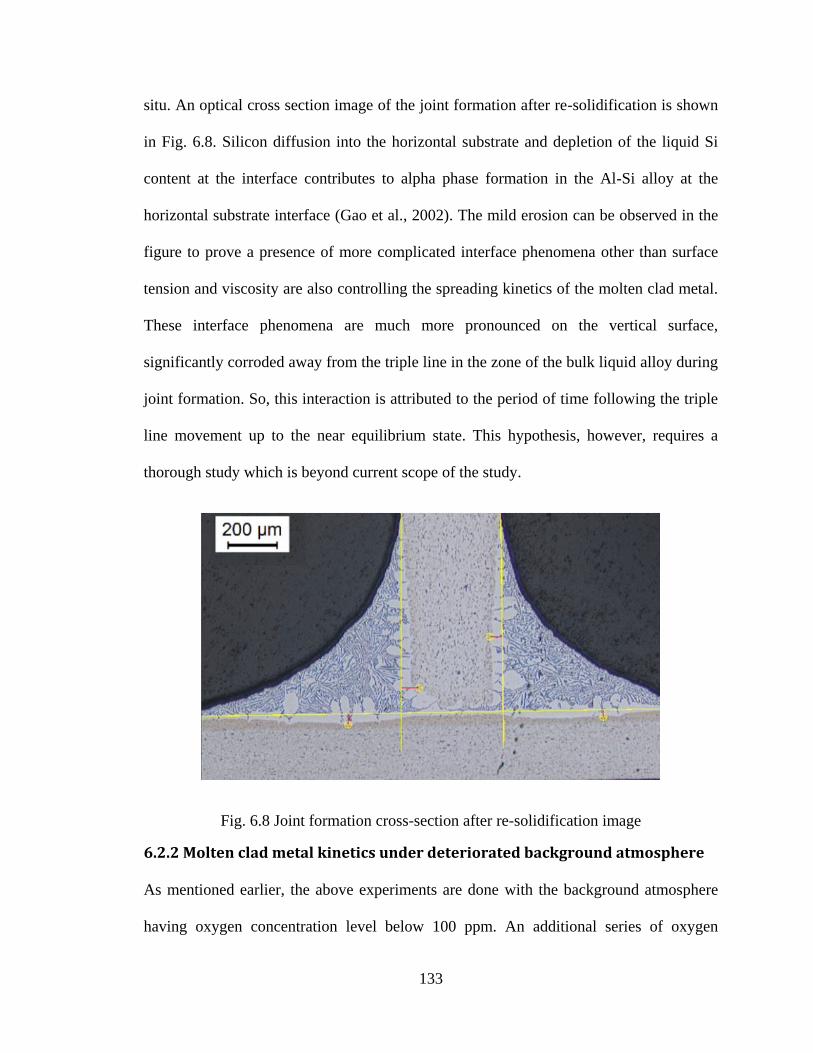
133
situ. An optical cross section image of the joint formation after re-solidification is shown
in Fig. 6.8. Silicon diffusion into the horizontal substrate and depletion of the liquid Si
content at the interface contributes to alpha phase formation in the Al-Si alloy at the
horizontal substrate interface (Gao et al., 2002). The mild erosion can be observed in the
figure to prove a presence of more complicated interface phenomena other than surface
tension and viscosity are also controlling the spreading kinetics of the molten clad metal.
These interface phenomena are much more pronounced on the vertical surface,
significantly corroded away from the triple line in the zone of the bulk liquid alloy during
joint formation. So, this interaction is attributed to the period of time following the triple
line movement up to the near equilibrium state. This hypothesis, however, requires a
thorough study which is beyond current scope of the study.
Fig. 6.8 Joint formation cross-section after re-solidification image
6.2.2 Molten clad metal kinetics under deteriorated background atmosphere
As mentioned earlier, the above experiments are done with the background atmosphere
having oxygen concentration level below 100 ppm. An additional series of oxygen
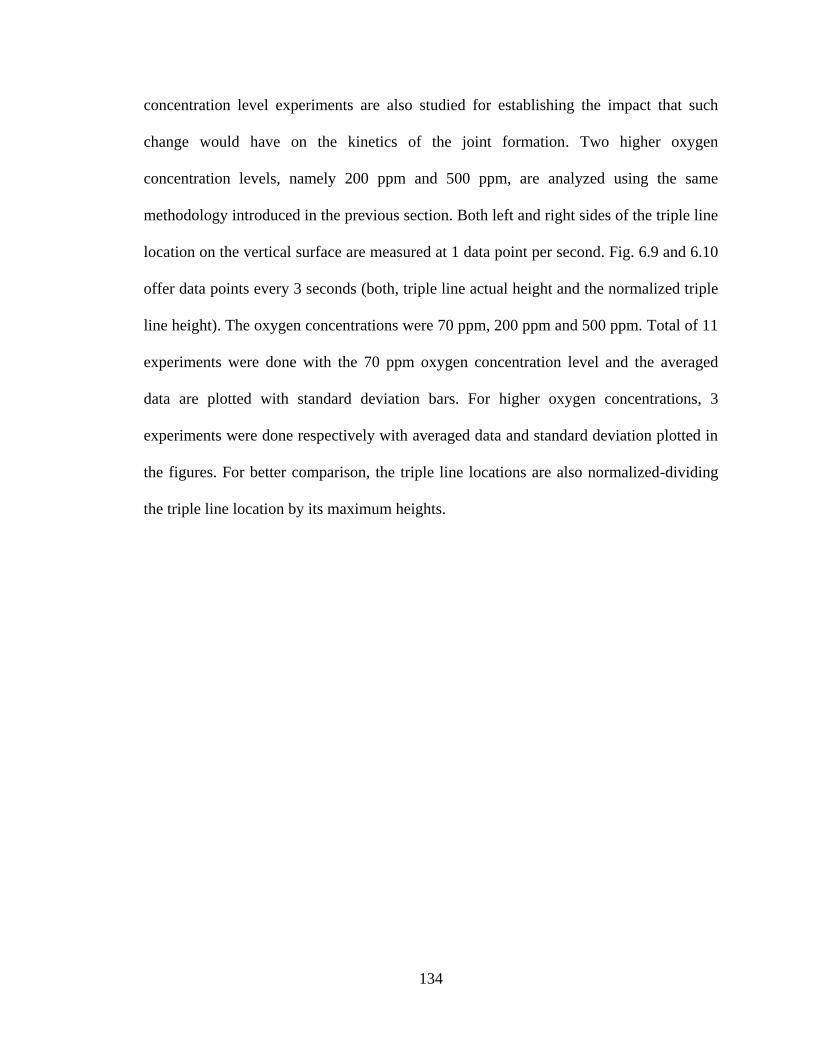
134
concentration level experiments are also studied for establishing the impact that such
change would have on the kinetics of the joint formation. Two higher oxygen
concentration levels, namely 200 ppm and 500 ppm, are analyzed using the same
methodology introduced in the previous section. Both left and right sides of the triple line
location on the vertical surface are measured at 1 data point per second. Fig. 6.9 and 6.10
offer data points every 3 seconds (both, triple line actual height and the normalized triple
line height). The oxygen concentrations were 70 ppm, 200 ppm and 500 ppm. Total of 11
experiments were done with the 70 ppm oxygen concentration level and the averaged
data are plotted with standard deviation bars. For higher oxygen concentrations, 3
experiments were done respectively with averaged data and standard deviation plotted in
the figures. For better comparison, the triple line locations are also normalized-dividing
the triple line location by its maximum heights.
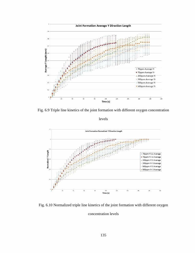
135
Fig. 6.9 Triple line kinetics of the joint formation with different oxygen concentration
levels
Fig. 6.10 Normalized triple line kinetics of the joint formation with different oxygen
concentration levels
136
Based on the results, it is noted that with higher oxygen content in the controlled brazing
atmosphere, the time consumed for the finishing joint formation is longer. However the
final height doesn’t have the dramatic difference compared to the 70 ppm oxygen level. It
can be seen that in these three oxygen level experiments, the initial kinetics behaviors are
close to each other. The deviation of the kinetics starts after initial 15 seconds with the
lowest triple line location in the 500 ppm oxygen level. To form the same joint area, 70
ppm oxygen level is clearly the optimal atmosphere condition for the triple line kinetics.
In terms of the final triple line location height, the difference between 200 ppm and 500
ppm is not dramatic with the standard deviation bars. No clear distinction between the
200 and 500 ppm’s can be identified. This may be an artifact of the relatively small
number of tests performed. The clear distinction between these two deteriorated cases vs.
70 ppm is, however, obvious.
6.2.3 Molten clad metal kinetics with different clad layer thicknesses
As mentioned earlier, the 0.03 mm thickness clad metal sample configuration is the
benchmark for further investigation on the clad metal thickness impact. Two more clad
metal thicknesses (0.4 mm and 0.8 mm) are also considered, see Fig. 6.1 (b) and (c). A
sample of 0.4 mm thickness TrilliumTM clad configuration is shown in Fig. 6.11.
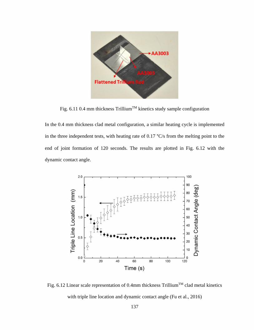
137
Fig. 6.11 0.4 mm thickness TrilliumTM kinetics study sample configuration
In the 0.4 mm thickness clad metal configuration, a similar heating cycle is implemented
in the three independent tests, with heating rate of 0.17 °C/s from the melting point to the
end of joint formation of 120 seconds. The results are plotted in Fig. 6.12 with the
dynamic contact angle.
Fig. 6.12 Linear scale representation of 0.4mm thickness TrilliumTM clad metal kinetics
with triple line location and dynamic contact angle (Fu et al., 2016)
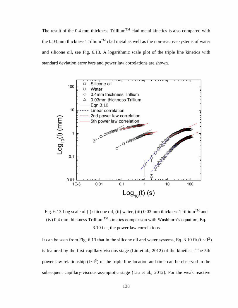
138
The result of the 0.4 mm thickness TrilliumTM clad metal kinetics is also compared with
the 0.03 mm thickness TrilliumTM clad metal as well as the non-reactive systems of water
and silicone oil, see Fig. 6.13. A logarithmic scale plot of the triple line kinetics with
standard deviation error bars and power law correlations are shown.
Fig. 6.13 Log scale of (i) silicone oil, (ii) water, (iii) 0.03 mm thickness TrilliumTM and
(iv) 0.4 mm thickness TrilliumTM kinetics comparison with Washburn’s equation, Eq.
3.10 i.e., the power law correlations
It can be seen from Fig. 6.13 that in the silicone oil and water systems, Eq. 3.10 fit (t ~ l2)
is featured by the first capillary-viscous stage (Liu et al., 2012) of the kinetics. The 5th
power law relationship (t~l5) of the triple line location and time can be observed in the
subsequent capillary-viscous-asymptotic stage (Liu et al., 2012). For the weak reactive
139
wetting case of TrilliumTM clad metal, a linear power law correlation ( t~l) can be
observed in experiments of both 0.03 mm thickness and 0.4 mm thickness liquid clad
metal. A 2nd power law correlation can be fitted in the second stage (Fu et al., 2013).
Equation 3.10 (with only viscosity and surface tension as dominating factors) would not
be adequate to explain the two-stage phenomenon. This is because additional physical
phenomena (such as chemical reaction, ridging, inter-diffusion and de-oxidation of the
liquid Trillium as well as dissolution of TrilliumTM on aluminum substrate) also play
significant roles in the process (Saiz et al., 1998; Saiz et al., 2005; Saiz et al., 2007;
Benhassine et al., 2009; Champion et al., 1969; Drevet et al., 2012), especially at the
triple line location.
To further study the triple line kinetics impact factors, 0.8 mm thickness clad metal
configuration (Fig. 6.1) is used as well, with a higher heating rate of 0.22 °C/s (from the
melting point to the end of joint formation of 120 seconds). Two independent tests are
done, and the averaged values of the triple line location with standard deviation error bars
are shown in the linear scale in Fig. 6.14 and the log scale in Fig. 6.15.
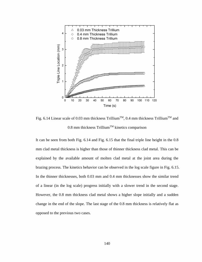
140
Fig. 6.14 Linear scale of 0.03 mm thickness TrilliumTM, 0.4 mm thickness TrilliumTM and
0.8 mm thickness TrilliumTM kinetics comparison
It can be seen from both Fig. 6.14 and Fig. 6.15 that the final triple line height in the 0.8
mm clad metal thickness is higher than those of thinner thickness clad metal. This can be
explained by the available amount of molten clad metal at the joint area during the
brazing process. The kinetics behavior can be observed in the log scale figure in Fig. 6.15.
In the thinner thicknesses, both 0.03 mm and 0.4 mm thicknesses show the similar trend
of a linear (in the log scale) progress initially with a slower trend in the second stage.
However, the 0.8 mm thickness clad metal shows a higher slope initially and a sudden
change in the end of the slope. The last stage of the 0.8 mm thickness is relatively flat as
opposed to the previous two cases.
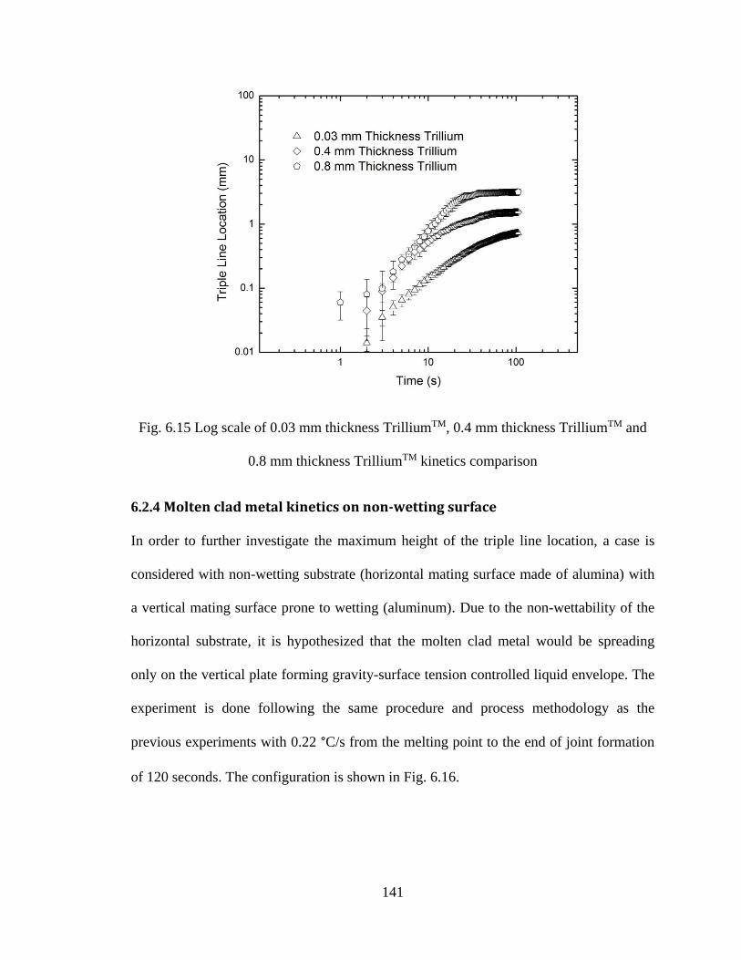
141
Fig. 6.15 Log scale of 0.03 mm thickness TrilliumTM, 0.4 mm thickness TrilliumTM and
0.8 mm thickness TrilliumTM kinetics comparison
6.2.4 Molten clad metal kinetics on non-wetting surface
In order to further investigate the maximum height of the triple line location, a case is
considered with non-wetting substrate (horizontal mating surface made of alumina) with
a vertical mating surface prone to wetting (aluminum). Due to the non-wettability of the
horizontal substrate, it is hypothesized that the molten clad metal would be spreading
only on the vertical plate forming gravity-surface tension controlled liquid envelope. The
experiment is done following the same procedure and process methodology as the
previous experiments with 0.22 °C/s from the melting point to the end of joint formation
of 120 seconds. The configuration is shown in Fig. 6.16.
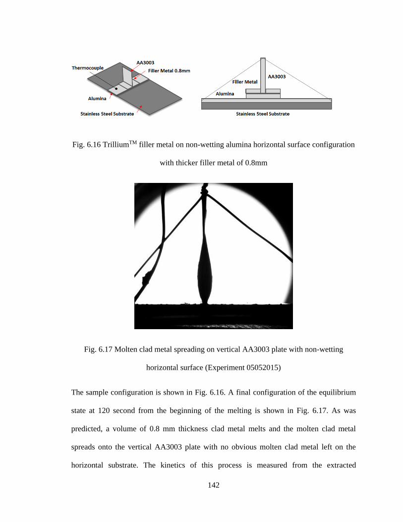
142
Fig. 6.16 TrilliumTM filler metal on non-wetting alumina horizontal surface configuration
with thicker filler metal of 0.8mm
Fig. 6.17 Molten clad metal spreading on vertical AA3003 plate with non-wetting
horizontal surface (Experiment 05052015)
The sample configuration is shown in Fig. 6.16. A final configuration of the equilibrium
state at 120 second from the beginning of the melting is shown in Fig. 6.17. As was
predicted, a volume of 0.8 mm thickness clad metal melts and the molten clad metal
spreads onto the vertical AA3003 plate with no obvious molten clad metal left on the
horizontal substrate. The kinetics of this process is measured from the extracted
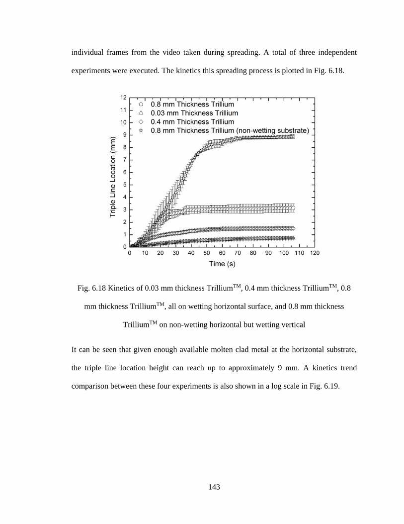
143
individual frames from the video taken during spreading. A total of three independent
experiments were executed. The kinetics this spreading process is plotted in Fig. 6.18.
Fig. 6.18 Kinetics of 0.03 mm thickness TrilliumTM, 0.4 mm thickness TrilliumTM, 0.8
mm thickness TrilliumTM, all on wetting horizontal surface, and 0.8 mm thickness
TrilliumTM on non-wetting horizontal but wetting vertical
It can be seen that given enough available molten clad metal at the horizontal substrate,
the triple line location height can reach up to approximately 9 mm. A kinetics trend
comparison between these four experiments is also shown in a log scale in Fig. 6.19.
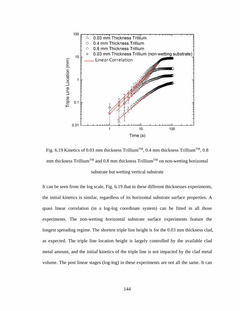
144
Fig. 6.19 Kinetics of 0.03 mm thickness TrilliumTM, 0.4 mm thickness TrilliumTM, 0.8
mm thickness TrilliumTM and 0.8 mm thickness TrilliumTM on non-wetting horizontal
substrate but wetting vertical substrate
It can be seen from the log scale, Fig. 6.19 that in these different thicknesses experiments,
the initial kinetics is similar, regardless of its horizontal substrate surface properties. A
quasi linear correlation (in a log-log coordinate system) can be fitted in all those
experiments. The non-wetting horizontal substrate surface experiments feature the
longest spreading regime. The shortest triple line height is for the 0.03 mm thickness clad,
as expected. The triple line location height is largely controlled by the available clad
metal amount, and the initial kinetics of the triple line is not impacted by the clad metal
volume. The post linear stages (log-log) in these experiments are not all the same. It can
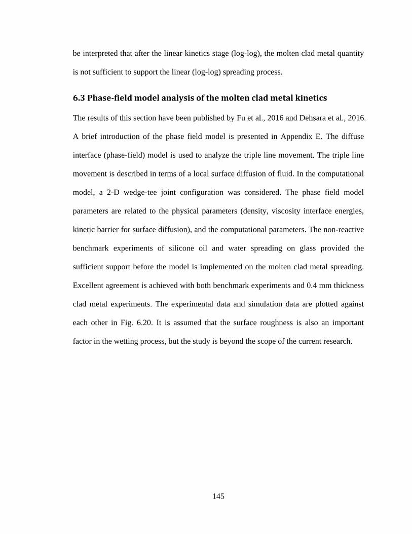
145
be interpreted that after the linear kinetics stage (log-log), the molten clad metal quantity
is not sufficient to support the linear (log-log) spreading process.
6.3 Phase-field model analysis of the molten clad metal kinetics
The results of this section have been published by Fu et al., 2016 and Dehsara et al., 2016.
A brief introduction of the phase field model is presented in Appendix E. The diffuse
interface (phase-field) model is used to analyze the triple line movement. The triple line
movement is described in terms of a local surface diffusion of fluid. In the computational
model, a 2-D wedge-tee joint configuration was considered. The phase field model
parameters are related to the physical parameters (density, viscosity interface energies,
kinetic barrier for surface diffusion), and the computational parameters. The non-reactive
benchmark experiments of silicone oil and water spreading on glass provided the
sufficient support before the model is implemented on the molten clad metal spreading.
Excellent agreement is achieved with both benchmark experiments and 0.4 mm thickness
clad metal experiments. The experimental data and simulation data are plotted against
each other in Fig. 6.20. It is assumed that the surface roughness is also an important
factor in the wetting process, but the study is beyond the scope of the current research.
146
Fig. 6.20 The comparison between experimental data and phase field modeling
6.4 Summary
In this chapter, the kinetics of molten clad metal at elevated temperatures spreading at the
wedge-tee joint area is studied comparatively both experimentally and numerically. A
thinner clad metal sample configuration is firstly established for the initial experiment
methodology. The result shows a slower triple line kinetics process compared to previous
non-reactive spreading process. Following the benchmark methodology, two additional
clad metal thicknesses are designed for experiments. The result shows the triple line
location height is impacted by the available amount of the molten clad metal at elevated
temperatures. Another non-wetting substrate is used as the ideal maximum amount
molten clad metal provided at the joint area. The result further confirms the triple line
location height is impacted by the molten clad metal volume. The comparative study also
shows the initial stages of these different configurations obey a similar quasi-linear
147
kinetics process regardless of its horizontal surface properties and its clad metal volumes.
With larger amount of the molten clad metal, the quasi-linear kinetics process in the log-
log scale lasts longer.
In the numerical analysis based on the result from Washington State University, a phase
field model of wetting based on modified Navier-Stokes equations, incompressibility
condition and the 4th order Cahn-Hilliard diffusion equation for the conserved phase field
is developed combining multiphase flow and contact line dynamics of a diffusive
boundary interface. The model provides a solid background for an accurate theoretical
description of the wetting phenomena for both non-reactive and reactive wetting at
elevated temperatures. The numerical model results are compared with the non-reactive
benchmark experiment results, and the results have an excellent agreement. Due to the
generality and thermodynamics nature of the model, this model can be extended to
complex problems with chemical reactions and diffusion of components, such as the
molten clad metal kinetics process. The numerical model successfully predicted the
evolution of the meniscus and triple line kinetics process for both non-reactive and
reactive systems.
148
CHAPTER 7: CONCLUSION AND FUTURE WORK
This chapter summarizes this dissertation. Contributions to the knowledge about kinetics
of spreading phenomena are addressed first. Suggestions regarding future study are
discussed next.
7.1 Main conclusions from the current study
The kinetics of non-reactive and reactive spreading for both ambient temperature systems
and the elevated temperature systems have been studied experimentally and compared to
numerically obtained data from a simultaneously performed collaborative study
constituting jointly a work within the NSF sponsored research under Grant # 1234581
and # 1235759. The kinetics of molten clad metal spreading is defined as the movement
of the triple line of the advancing front of the liquid metal driven by surface tension into
the joint area of two melting metal surfaces. This phenomenon is important for
Controlled Atmosphere Brazing (CAB) among multiple other technological applications.
Based on the experiment findings, the spreading kinetics at the wedge-tee joint area can
be well predicted via analytical empirical and semi-empirical correlations. The numerical
solutions for both non-reactive and reactive spreading has been obtained following a
development of the phase-field theory of the liquid front advances (that segment of work
is beyond the scope of the dissertation effort), except as data base for comparison.
The non-reactive spreading systems involved water on glass and silicone oil on glass. The
empirical data from these experiments were used to verify the analytical and the semi-
empirical solutions, as well as later numerical analysis.
The spreading kinetics at elevated temperatures features an Al-Si alloy system combined
with addition of KxFyAlz system on Al substrate.
149
The result of the non-reactive systems’ spreading has confirmed that the kinetics of
the triple line is controlled by surface tension and viscous force. An empirical constant
based on the Washburn’s law is established for both water and silicone oil systems. The
equilibrium height of the triple line location and contact angle relation from the
experiment data were both well predicted by the analytical solution derived from
Young’s and Laplace equation. Seebergh and Jiang’s empirical correlation well fitted in
the experimental data of spreading kinetics of capillary number and dynamic contact
angle in the silicone oil/glass systems. A modified Seebergh empirical correlation is also
developed to predict the capillary number and dynamic contact angle relationship from
the benchmark experiment in water/glass systems. The later capillary-viscous-asymptotic
stage is also discovered in both water/glass and silicone oil/glass systems. The later stage
obeys a 5th power law relationship consistently.
The sessile drop experiments for the molten clad metal spreading at elevated
temperatures have been designed to investigate the molten clad metal properties. The
system used is a new brazing clad metal material TrilliumTM, a patented Al-Si alloy with
embedded salt content so a self-fluxing process occurs during CAB brazing. The sessile
drop experiments were conducted with the Optical Contact angle Analyzer (OCA)
facility. The surface tension of the molten clad metal system has been experimentally
determined. The experimental data on kinetics of the molten metal triple line movement
were compared with kinetics trends from various literature sources. The re-solidification
images and SEM/EDS results indicating the structures at the interface zone within the
triple line region prove that the molten clad metal spreading at elevated temperatures
involves more complicated physical phenomena, such as inter-diffusion and dissolution.
150
Still, the interaction may be considered as mild if the dwell at the peak temperature is
brief.
Various clad metal thicknesses (before melting – hence offering various liquid pool
quantities during spreading) were considered in the experiments to determine the joint
formation size. The linear log-log kinetics correlation is identified in the experiment data,
and a 2nd power law correlation is observed in the later stage. A non-wetting alumina
horizontal substrate and vertical AA3003 plate system was studied as well to establish
kinetics of the triple line on the vertical Al3003 surface. The results re-emphases that clad
liquid metal initial volume impacts the final triple line location height. The initial log-log
kinetics relationship is established, but the larger the clad metal volume, the longer the
linear log-log trend lasts. The later stages of the kinetics are not all the same due to
complex controlling factors.
Supported by the experimental results from both non-reactive and reactive systems, a
phase field model was established in a simultaneous study, beyond the scope of the
Thesis work (that one is executed at the Washington State University). Based on
Lowengrub et al. (1998) analysis and the initial model from Jacqmin (2000), the
governing equations of the incompressible model were offered. These consist of the
modified Navier-Stokes equations, the incompressibility condition and the 4th order
Cahn-Hilliard diffusion equation. The numerical model is simulated by using Comsol
MultiPhysics 3.5a/4.3 software. The simulated meniscus well verifies the experimental
meniscus in both non-reactive and reactive systems. The numerical results have excellent
agreement with the triple line kinetics in water/glass, silicone/glass and 0.4 mm molten
clad metal on AA3003. Besides the surface tension and viscous force dominating the
151
non-reactive systems, it is assumed that diffusion controlled concentration changes do not
significantly affect the fluid viscosity in the reactive systems at elevated temperatures,
and that their effect on the TPL mobility can be phenomenologically included in the
model through the triple line mobility parameter without explicitly modeling the changes
in diffusion and concentration of molten clad metal.
7.2 Future work
Further study is necessary to better understand the physical/chemical nature of the
spreading process of liquid metal over metal substrate.
In the non-reactive ambient temperature benchmark study, two liquid systems are
investigated to support the surface tension and viscous force driven theory and the
numerical model verified the experimental results. More liquid species spreading would
be helpful to identify the later stages of the spreading kinetics phenomena. The initial
stage of the non-reactive spreading can be identified as the Washburn type spreading, but
the process ending point to the later stage is still ambiguous. An empirical relationship of
the transition between Washburn type spreading and the capillary-viscous-asymptotic
stage should be established either from experimental analysis or numerical analysis.
The clad metal sessile drop kinetics needs to be studied further in the current
experimental setup in both non-wetting and wetting substrates. It is noticed that in the
current experiments the spreading process is controlled by different physical phenomena
in these two types of substrates. Dissolution, inter-diffusion and are dominant in the case
of the wetting Al substrate.
152
The exact triple line location height at equilibrium state needs to be confirmed with liquid
molten clad metal on the wetting substrate not limited.
Surface topography has been an important factor impacting the spreading kinetics. In
current study, smooth surfaces are considered in both non-reactive and reactive spreading
kinetics study. Surface roughness should be identified as another variable in the future
study.
Temperature heating rate impact on the kinetics of the spreading at elevated temperatures
has been noticed in several experiments that are not reported here. Smaller heating rate
corresponds to the slower triple line growth with smaller value in the spreading kinetics
correlation slope. The correlation between the heating rate and the diffusion of the mobile
elements in the aluminum alloy should be further identified. To what extent the heating
rate is impacting the kinetics of spreading should be investigated.
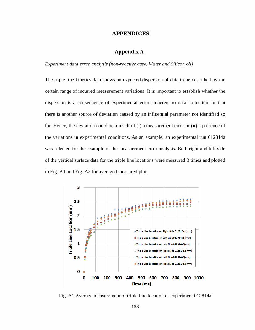
153
APPENDICES
Appendix A
Experiment data error analysis (non-reactive case, Water and Silicon oil)
The triple line kinetics data shows an expected dispersion of data to be described by the
certain range of incurred measurement variations. It is important to establish whether the
dispersion is a consequence of experimental errors inherent to data collection, or that
there is another source of deviation caused by an influential parameter not identified so
far. Hence, the deviation could be a result of (i) a measurement error or (ii) a presence of
the variations in experimental conditions. As an example, an experimental run 012814a
was selected for the example of the measurement error analysis. Both right and left side
of the vertical surface data for the triple line locations were measured 3 times and plotted
in Fig. A1 and Fig. A2 for averaged measured plot.
Fig. A1 Average measurement of triple line location of experiment 012814a
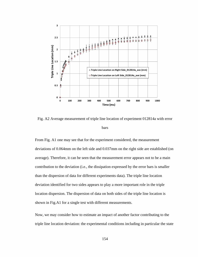
154
Fig. A2 Average measurement of triple line location of experiment 012814a with error
bars
From Fig. A1 one may see that for the experiment considered, the measurement
deviations of 0.064mm on the left side and 0.037mm on the right side are established (on
average). Therefore, it can be seen that the measurement error appears not to be a main
contribution to the deviation (i.e., the dissipation expressed by the error bars is smaller
than the dispersion of data for different experiments data). The triple line location
deviation identified for two sides appears to play a more important role in the triple
location dispersion. The dispersion of data on both sides of the triple line location is
shown in Fig.A1 for a single test with different measurements.
Now, we may consider how to estimate an impact of another factor contributing to the
triple line location deviation: the experimental conditions including in particular the state
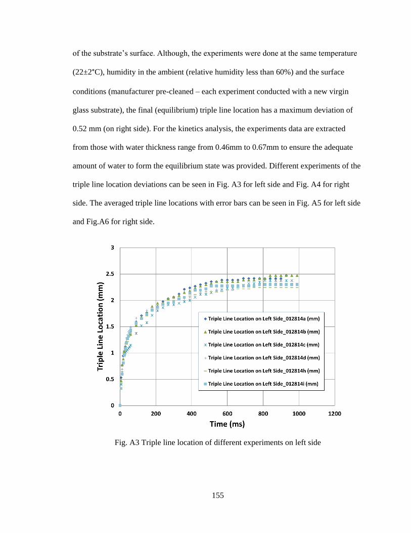
155
of the substrate’s surface. Although, the experiments were done at the same temperature
(22±2°C), humidity in the ambient (relative humidity less than 60%) and the surface
conditions (manufacturer pre-cleaned – each experiment conducted with a new virgin
glass substrate), the final (equilibrium) triple line location has a maximum deviation of
0.52 mm (on right side). For the kinetics analysis, the experiments data are extracted
from those with water thickness range from 0.46mm to 0.67mm to ensure the adequate
amount of water to form the equilibrium state was provided. Different experiments of the
triple line location deviations can be seen in Fig. A3 for left side and Fig. A4 for right
side. The averaged triple line locations with error bars can be seen in Fig. A5 for left side
and Fig.A6 for right side.
Fig. A3 Triple line location of different experiments on left side
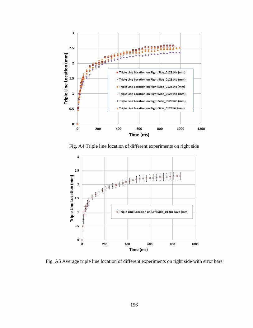
156
Fig. A4 Triple line location of different experiments on right side
Fig. A5 Average triple line location of different experiments on right side with error bars
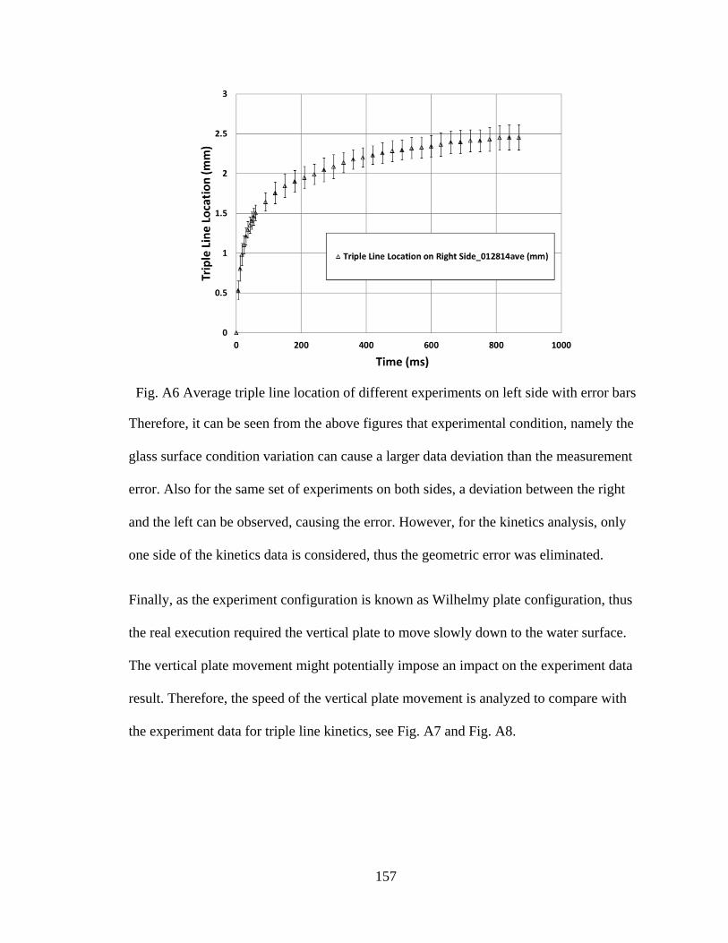
157
Fig. A6 Average triple line location of different experiments on left side with error bars
Therefore, it can be seen from the above figures that experimental condition, namely the
glass surface condition variation can cause a larger data deviation than the measurement
error. Also for the same set of experiments on both sides, a deviation between the right
and the left can be observed, causing the error. However, for the kinetics analysis, only
one side of the kinetics data is considered, thus the geometric error was eliminated.
Finally, as the experiment configuration is known as Wilhelmy plate configuration, thus
the real execution required the vertical plate to move slowly down to the water surface.
The vertical plate movement might potentially impose an impact on the experiment data
result. Therefore, the speed of the vertical plate movement is analyzed to compare with
the experiment data for triple line kinetics, see Fig. A7 and Fig. A8.
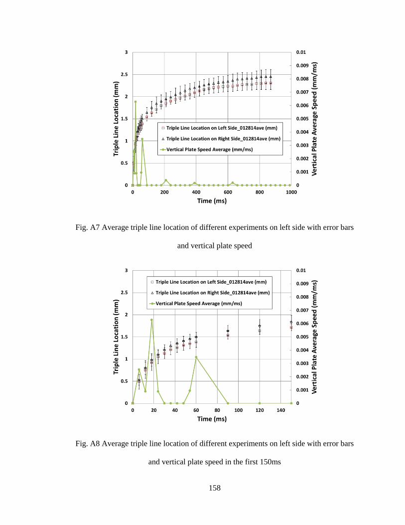
158
Fig. A7 Average triple line location of different experiments on left side with error bars
and vertical plate speed
Fig. A8 Average triple line location of different experiments on left side with error bars
and vertical plate speed in the first 150ms
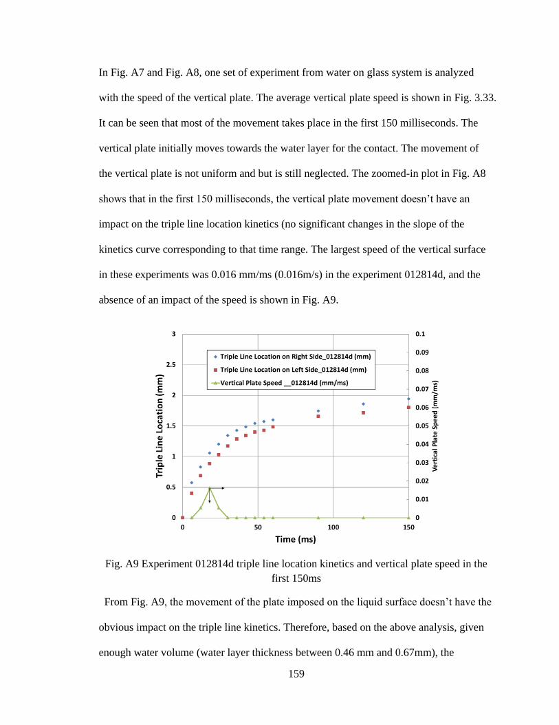
159
In Fig. A7 and Fig. A8, one set of experiment from water on glass system is analyzed
with the speed of the vertical plate. The average vertical plate speed is shown in Fig. 3.33.
It can be seen that most of the movement takes place in the first 150 milliseconds. The
vertical plate initially moves towards the water layer for the contact. The movement of
the vertical plate is not uniform and but is still neglected. The zoomed-in plot in Fig. A8
shows that in the first 150 milliseconds, the vertical plate movement doesn’t have an
impact on the triple line location kinetics (no significant changes in the slope of the
kinetics curve corresponding to that time range. The largest speed of the vertical surface
in these experiments was 0.016 mm/ms (0.016m/s) in the experiment 012814d, and the
absence of an impact of the speed is shown in Fig. A9.
Fig. A9 Experiment 012814d triple line location kinetics and vertical plate speed in the
first 150ms
From Fig. A9, the movement of the plate imposed on the liquid surface doesn’t have the
obvious impact on the triple line kinetics. Therefore, based on the above analysis, given
enough water volume (water layer thickness between 0.46 mm and 0.67mm), the
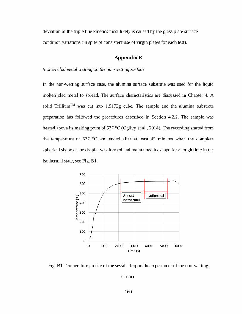
160
deviation of the triple line kinetics most likely is caused by the glass plate surface
condition variations (in spite of consistent use of virgin plates for each test).
Appendix B
Molten clad metal wetting on the non-wetting surface
In the non-wetting surface case, the alumina surface substrate was used for the liquid
molten clad metal to spread. The surface characteristics are discussed in Chapter 4. A
solid TrilliumTM was cut into 1.5173g cube. The sample and the alumina substrate
preparation has followed the procedures described in Section 4.2.2. The sample was
heated above its melting point of 577 °C (Ogilvy et al., 2014). The recording started from
the temperature of 577 °C and ended after at least 45 minutes when the complete
spherical shape of the droplet was formed and maintained its shape for enough time in the
isothermal state, see Fig. B1.
Fig. B1 Temperature profile of the sessile drop in the experiment of the non-wetting
surface
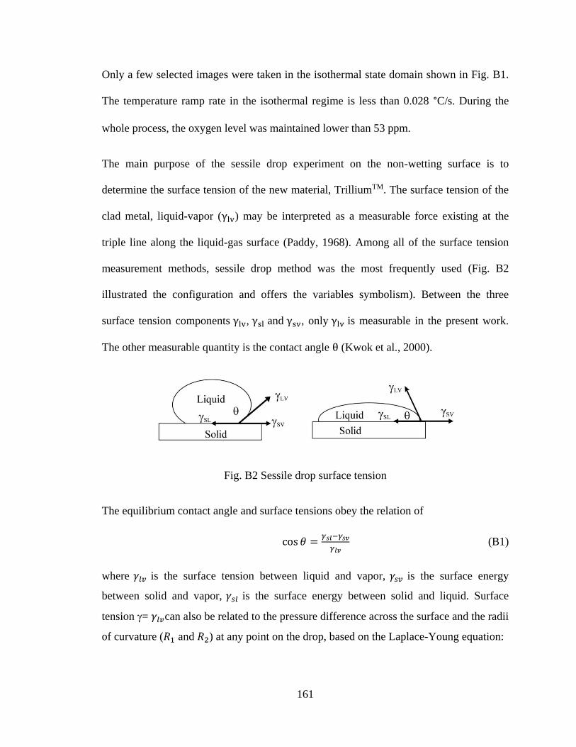
161
Only a few selected images were taken in the isothermal state domain shown in Fig. B1.
The temperature ramp rate in the isothermal regime is less than 0.028 °C/s. During the
whole process, the oxygen level was maintained lower than 53 ppm.
The main purpose of the sessile drop experiment on the non-wetting surface is to
determine the surface tension of the new material, TrilliumTM. The surface tension of the
clad metal, liquid-vapor (γlv) may be interpreted as a measurable force existing at the
triple line along the liquid-gas surface (Paddy, 1968). Among all of the surface tension
measurement methods, sessile drop method was the most frequently used (Fig. B2
illustrated the configuration and offers the variables symbolism). Between the three
surface tension components γlv, γsl and γsv, only γlv is measurable in the present work.
The other measurable quantity is the contact angle θ (Kwok et al., 2000).
Fig. B2 Sessile drop surface tension
The equilibrium contact angle and surface tensions obey the relation of
cos 𝜃 =𝛾𝑠𝑙−𝛾𝑠𝑣
𝛾𝑙𝑣 (B1)
where 𝛾𝑙𝑣 is the surface tension between liquid and vapor, 𝛾𝑠𝑣 is the surface energy
between solid and vapor, 𝛾𝑠𝑙 is the surface energy between solid and liquid. Surface
tension = 𝛾𝑙𝑣can also be related to the pressure difference across the surface and the radii
of curvature (𝑅1 and 𝑅2) at any point on the drop, based on the Laplace-Young equation:
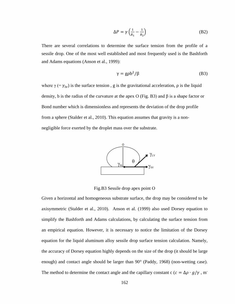
162
∆𝑃 = 𝛾 (1
𝑅1−
1
𝑅2) (B2)
There are several correlations to determine the surface tension from the profile of a
sessile drop. One of the most well established and most frequently used is the Bashforth
and Adams equations (Anson et al., 1999):
γ = gρb2/β (B3)
where γ (= 𝛾𝑙𝑣) is the surface tension , g is the gravitational acceleration, ρ is the liquid
density, b is the radius of the curvature at the apex O (Fig. B3) and β is a shape factor or
Bond number which is dimensionless and represents the deviation of the drop profile
from a sphere (Stalder et al., 2010). This equation assumes that gravity is a non-
negligible force exerted by the droplet mass over the substrate.
Fig.B3 Sessile drop apex point O
Given a horizontal and homogeneous substrate surface, the drop may be considered to be
axisymmetric (Stalder et al., 2010). Anson et al. (1999) also used Dorsey equation to
simplify the Bashforth and Adams calculations, by calculating the surface tension from
an empirical equation. However, it is necessary to notice the limitation of the Dorsey
equation for the liquid aluminum alloy sessile drop surface tension calculation. Namely,
the accuracy of Dorsey equation highly depends on the size of the drop (it should be large
enough) and contact angle should be larger than 90° (Paddy, 1968) (non-wetting case).
The method to determine the contact angle and the capillary constant c (𝑐 = ∆𝜌 ∙ 𝑔/𝛾 , m-
163
2) is based on the on the low-bond axisymmetric drop shape analysis (LBADSA) (Stalder
et al., 2010). The method is implemented as a Java plug-in for the ImageJ software as
mentioned in Chapter 4. It needs to be pointed out that LBADSA method can only be
applied to small quasi-spherical drops whose diameter is of the order of magnitude of
millimeters as used in our tests. The ImageJ measurements were conducted multiple
times by using the region energy optimization option in the plug-in for the calculation of
the capillary constant value with a comparison between the values obtained from other
references (Anson et al., 1999; Guicoechea et al., 1992). The measured contact angle of
the molten clad metal on the alumina non-wetting surface is 131 °± 0.5 °. The measured
capillary constant is 6.42 × 10⁴ m-2.
The surface tension of the molten clad metal was tested by applying Dorsey equation
(Anson et al., 1999). The empirical relation, Dorsey's equation (Dorsey 1928), was
applied to calculate the surface tension of the clad metal alloy (Iida et al., 1988) (see Fig.
B4):
γlv = gρX2 (0.0520
f− 0.1227 + 0.0481f) (B4)
where 𝛾𝑙𝑣 is the surface tension, 𝑔 is the gravitational acceleration, 𝜌 is the density of the
liquid alloy, 𝑋 and 𝑌 are the experimental geometric parameters shown in Fig. B4, and
the Dorsey factor f is given by
𝑓 =𝑌
𝑋− 0.4142
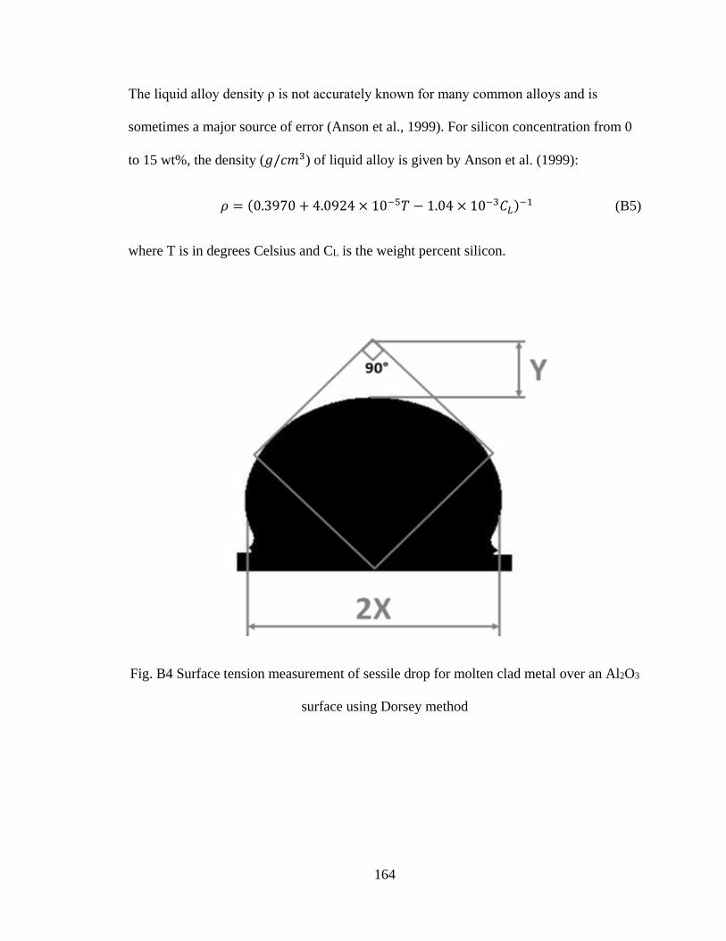
164
The liquid alloy density ρ is not accurately known for many common alloys and is
sometimes a major source of error (Anson et al., 1999). For silicon concentration from 0
to 15 wt%, the density (𝑔/𝑐𝑚3) of liquid alloy is given by Anson et al. (1999):
𝜌 = (0.3970 + 4.0924 × 10⁻⁵𝑇 − 1.04 × 10⁻³𝐶𝐿)−1 (B5)
where T is in degrees Celsius and CL is the weight percent silicon.
Fig. B4 Surface tension measurement of sessile drop for molten clad metal over an Al2O3
surface using Dorsey method
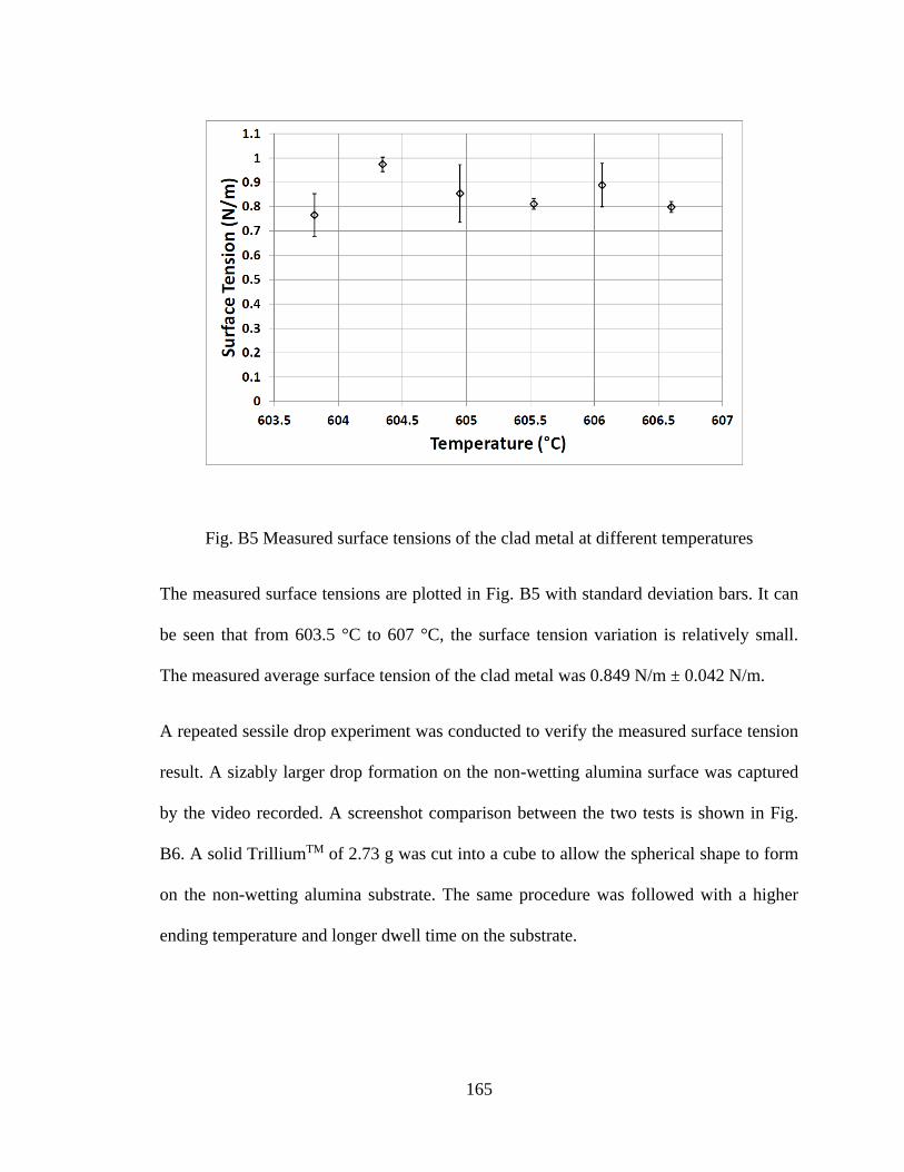
165
Fig. B5 Measured surface tensions of the clad metal at different temperatures
The measured surface tensions are plotted in Fig. B5 with standard deviation bars. It can
be seen that from 603.5 °C to 607 °C, the surface tension variation is relatively small.
The measured average surface tension of the clad metal was 0.849 N/m ± 0.042 N/m.
A repeated sessile drop experiment was conducted to verify the measured surface tension
result. A sizably larger drop formation on the non-wetting alumina surface was captured
by the video recorded. A screenshot comparison between the two tests is shown in Fig.
B6. A solid TrilliumTM of 2.73 g was cut into a cube to allow the spherical shape to form
on the non-wetting alumina substrate. The same procedure was followed with a higher
ending temperature and longer dwell time on the substrate.
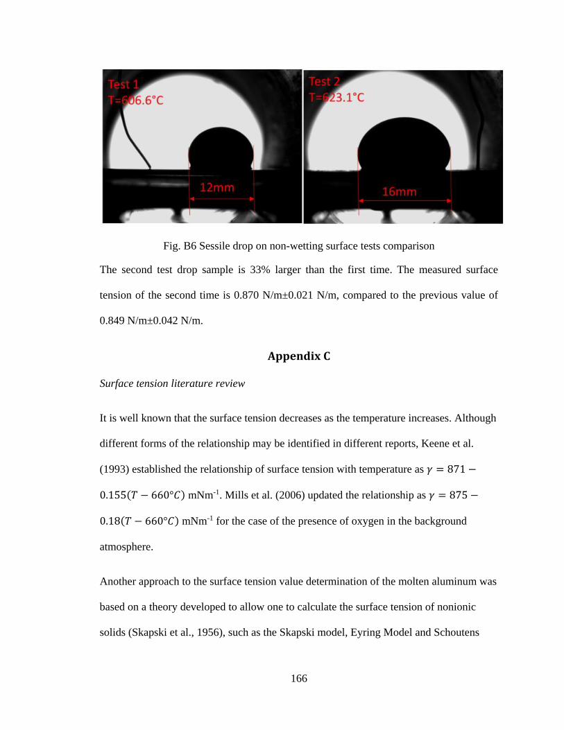
166
Fig. B6 Sessile drop on non-wetting surface tests comparison
The second test drop sample is 33% larger than the first time. The measured surface
tension of the second time is 0.870 N/m±0.021 N/m, compared to the previous value of
0.849 N/m±0.042 N/m.
Appendix C
Surface tension literature review
It is well known that the surface tension decreases as the temperature increases. Although
different forms of the relationship may be identified in different reports, Keene et al.
(1993) established the relationship of surface tension with temperature as 𝛾 = 871 −
0.155(𝑇 − 660°𝐶) mNm-1. Mills et al. (2006) updated the relationship as 𝛾 = 875 −
0.18(𝑇 − 660°𝐶) mNm-1 for the case of the presence of oxygen in the background
atmosphere.
Another approach to the surface tension value determination of the molten aluminum was
based on a theory developed to allow one to calculate the surface tension of nonionic
solids (Skapski et al., 1956), such as the Skapski model, Eyring Model and Schoutens
167
model, etc. The theoretical consideration is based on a classical statistical
thermodynamics formulation of Skapski et al. (1956), and Eyring and his coworkers
(Aqra et al., 2012). Based on these models, several modified version were developed. The
calculated values were of the order of 1000 mNm-1.The calculated values are higher than
the experimental values. The deviations in the experimental values lead to a decrease of
the surface tension due to the oxygen contamination. Since γsv and γsl were calculated
based on the definition of the contact angle (Kwok et al., 2000), and it is necessary to
point out that the methodology was actually applicable for a low temperature, non-metal
surface tension calculations. The situation for metals may be different, with the
continuous non-equilibrium state in molten metal in a presence of oxygen. Aqra et al.
(2012) compared their calculated results with the data reported from experiments (γlv) or
calculations (γsv), giving a surface tension relationship with temperature as γ = 985 −
0.275(T − 660°C) mJm-2 in the range of 660 to 927 °C. It should be noted that a
comprehensive calculation for aluminum alloys surface tension γlv, surface energy
γsvand crystal-melt interfacial energy γsl are still not available, although single surface
tension γlv calculation for alloys was often reported (Su et al., 2005). The surface
tensions of alumina and its alloys from various literature sources are listed in Table C1.
Table C1 (Continued) Surface tension 𝛾lv of aluminum and aluminum alloys
Metal
Type
𝜸𝐥𝐯
(mN/m) T (°C)
Gas
Condition Method Year Reference
Al 713±11 1650 N/A Sessile Drop 1997
Naidich et al., 1998
Al 846 800 N/A Sessile Drop 1999
Anson et al., 1999
Al 870 660 Vacuum Sessile Drop 1974
Eustathopoulos
et al., 1974
Al 520 700-820 N/A Capillary 1914 Flint et al.,
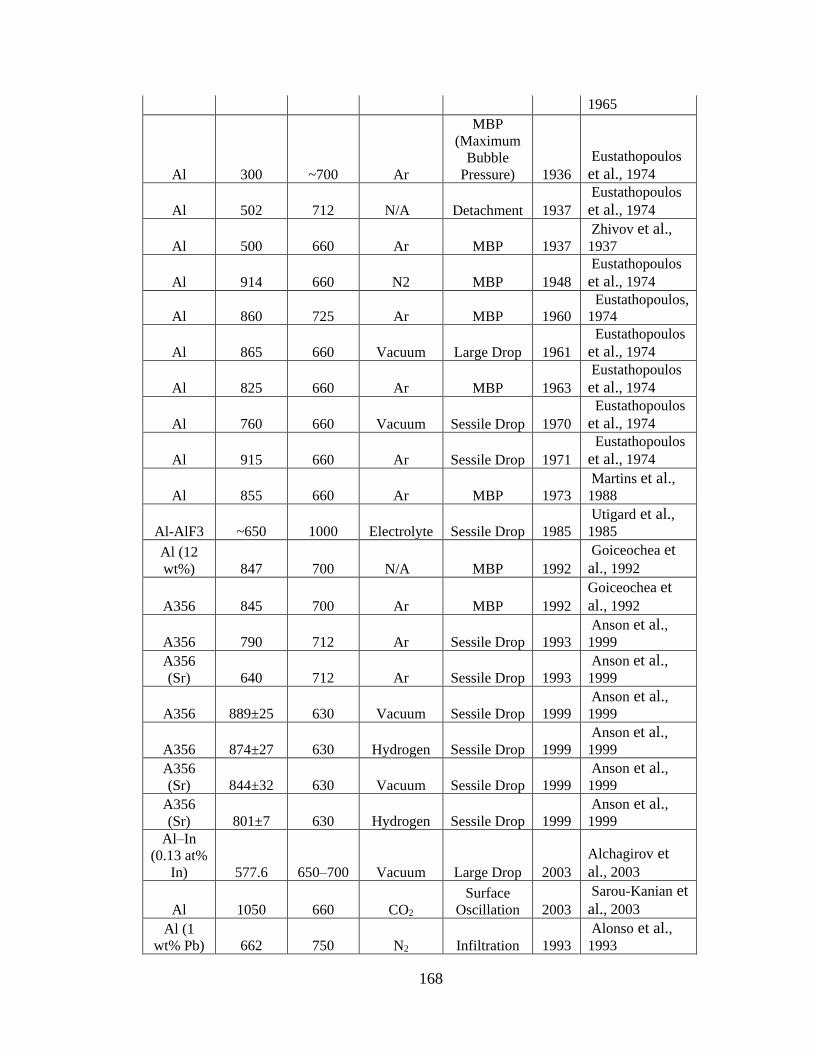
168
1965
Al 300 ~700 Ar
MBP
(Maximum
Bubble
Pressure) 1936
Eustathopoulos
et al., 1974
Al 502 712 N/A Detachment 1937
Eustathopoulos
et al., 1974
Al 500 660 Ar MBP 1937
Zhivov et al., 1937
Al 914 660 N2 MBP 1948
Eustathopoulos
et al., 1974
Al 860 725 Ar MBP 1960
Eustathopoulos,
1974
Al 865 660 Vacuum Large Drop 1961
Eustathopoulos
et al., 1974
Al 825 660 Ar MBP 1963
Eustathopoulos
et al., 1974
Al 760 660 Vacuum Sessile Drop 1970
Eustathopoulos
et al., 1974
Al 915 660 Ar Sessile Drop 1971
Eustathopoulos
et al., 1974
Al 855 660 Ar MBP 1973
Martins et al., 1988
Al-AlF3 ~650 1000 Electrolyte Sessile Drop 1985
Utigard et al., 1985
Al (12
wt%) 847 700 N/A MBP 1992
Goiceochea et
al., 1992
A356 845 700 Ar MBP 1992
Goiceochea et
al., 1992
A356 790 712 Ar Sessile Drop 1993
Anson et al., 1999
A356
(Sr) 640 712 Ar Sessile Drop 1993
Anson et al., 1999
A356 889±25 630 Vacuum Sessile Drop 1999
Anson et al., 1999
A356 874±27 630 Hydrogen Sessile Drop 1999
Anson et al., 1999
A356
(Sr) 844±32 630 Vacuum Sessile Drop 1999
Anson et al., 1999
A356
(Sr) 801±7 630 Hydrogen Sessile Drop 1999
Anson et al., 1999
Al–In
(0.13 at%
In) 577.6 650–700 Vacuum Large Drop 2003
Alchagirov et
al., 2003
Al 1050 660 CO2
Surface
Oscillation 2003
Sarou-Kanian et
al., 2003
Al (1
wt% Pb) 662 750 N2 Infiltration 1993
Alonso et al., 1993
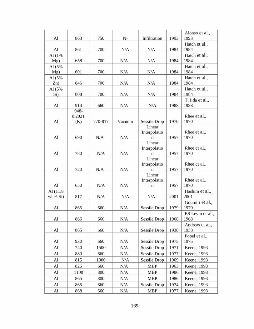
169
Al 863 750 N2 Infiltration 1993
Alonso et al., 1993
Al 861 700 N/A N/A 1984
Hatch et al., 1984
Al (1%
Mg) 658 700 N/A N/A 1984
Hatch et al., 1984
Al (5%
Mg) 601 700 N/A N/A 1984
Hatch et al., 1984
Al (5%
Zn) 846 700 N/A N/A 1984
Hatch et al., 1984
Al (5%
Si) 808 700 N/A N/A 1984
Hatch et al., 1984
Al 914 660 N/A N/A 1988
T. Iida et al., 1988
Al
948-
0.202T
(K) 770-817 Vacuum Sessile Drop 1970
Rhee et al., 1970
Al 690 N/A N/A
Linear
Interpolatio
n 1957
Rhee et al., 1970
Al 780 N/A N/A
Linear
Interpolatio
n 1957
Rhee et al., 1970
Al 720 N/A N/A
Linear
Interpolatio
n 1957
Rhee et al., 1970
Al 650 N/A N/A
Linear
Interpolatio
n 1957
Rhee et al., 1970
Al (11.8
wi % Si) 817 N/A N/A N/A 2001
Hashim et al., 2001
Al 865 660 N/A Sessile Drop 1979
Goumiri et al., 1979
Al 866 660 N/A Sessile Drop 1968
ES Levin et al., 1968
Al 865 660 N/A Sessile Drop 1938
Andreas et al., 1938
Al 930 660 N/A Sessile Drop 1975
Popel et al., 1975
Al 740 1500 N/A Sessile Drop 1971 Keene, 1993
Al 880 660 N/A Sessile Drop 1977 Keene, 1993
Al 815 1000 N/A Sessile Drop 1969 Keene, 1993
Al 825 660 N/A MBP 1963 Keene, 1993
Al 1100 800 N/A MBP 1986 Keene, 1993
Al 865 800 N/A MBP 1986 Keene, 1993
Al 865 660 N/A Sessile Drop 1974 Keene, 1993
Al 868 660 N/A MBP 1977 Keene, 1993
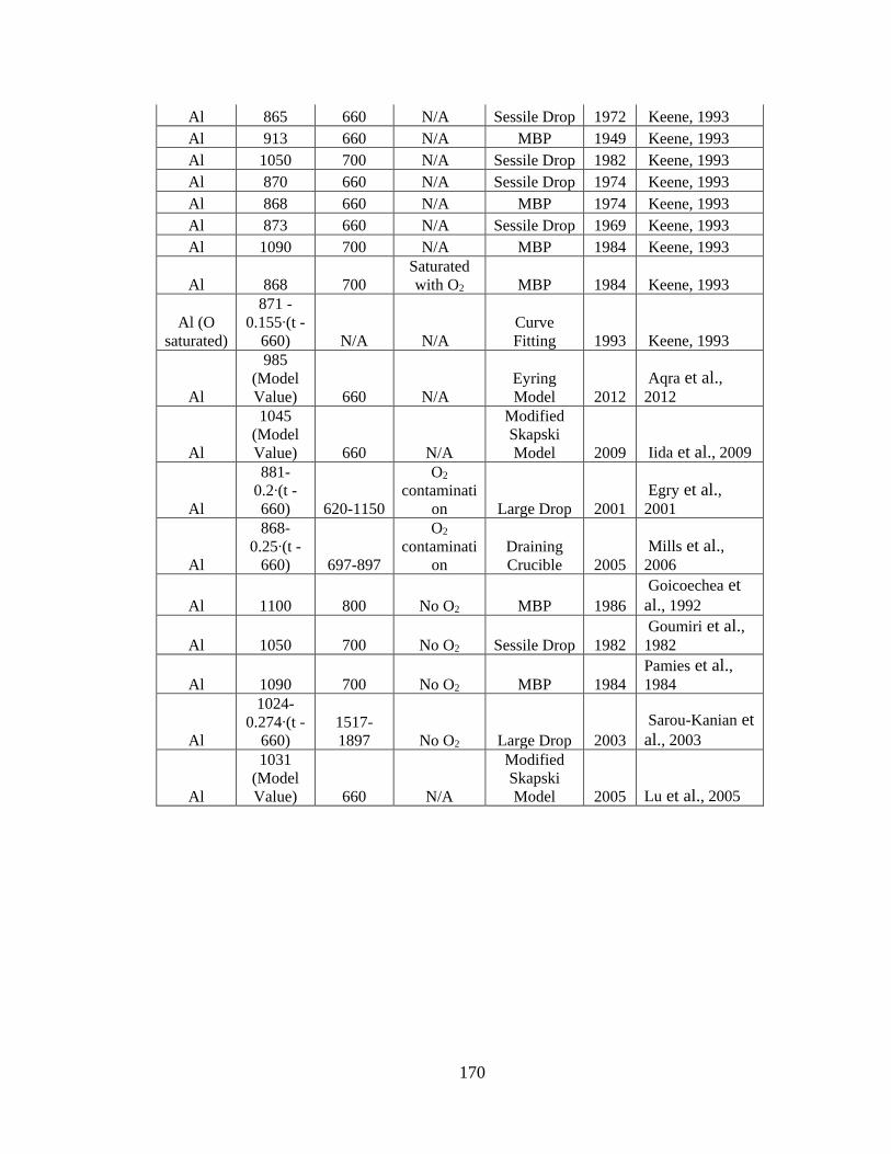
170
Al 865 660 N/A Sessile Drop 1972 Keene, 1993
Al 913 660 N/A MBP 1949 Keene, 1993
Al 1050 700 N/A Sessile Drop 1982 Keene, 1993
Al 870 660 N/A Sessile Drop 1974 Keene, 1993
Al 868 660 N/A MBP 1974 Keene, 1993
Al 873 660 N/A Sessile Drop 1969 Keene, 1993
Al 1090 700 N/A MBP 1984 Keene, 1993
Al 868 700
Saturated
with O2 MBP 1984 Keene, 1993
Al (O
saturated)
871 -
0.155∙(t -
660) N/A N/A
Curve
Fitting 1993 Keene, 1993
Al
985
(Model
Value) 660 N/A
Eyring
Model 2012
Aqra et al., 2012
Al
1045
(Model
Value) 660 N/A
Modified
Skapski
Model 2009 Iida et al., 2009
Al
881-
0.2∙(t -
660) 620-1150
O2
contaminati
on Large Drop 2001
Egry et al., 2001
Al
868-
0.25∙(t -
660) 697-897
O2
contaminati
on
Draining
Crucible 2005
Mills et al., 2006
Al 1100 800 No O2 MBP 1986
Goicoechea et
al., 1992
Al 1050 700 No O2 Sessile Drop 1982
Goumiri et al., 1982
Al 1090 700 No O2 MBP 1984
Pamies et al., 1984
Al
1024-
0.274∙(t -
660)
1517-
1897 No O2 Large Drop 2003
Sarou-Kanian et
al., 2003
Al
1031
(Model
Value) 660 N/A
Modified
Skapski
Model 2005 Lu et al., 2005
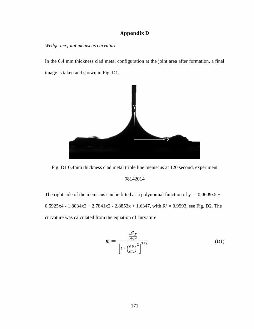
171
Appendix D
Wedge-tee joint meniscus curvature
In the 0.4 mm thickness clad metal configuration at the joint area after formation, a final
image is taken and shown in Fig. D1.
Fig. D1 0.4mm thickness clad metal triple line meniscus at 120 second, experiment
08142014
The right side of the meniscus can be fitted as a polynomial function of y = -0.0609x5 +
0.5925x4 - 1.8034x3 + 2.7841x2 - 2.8853x + 1.6347, with R² = 0.9993, see Fig. D2. The
curvature was calculated from the equation of curvature:
𝜅 =𝑑2𝑦
𝑑𝑥2
[1+(𝑑𝑦
𝑑𝑥)
2]
3/2 (D1)
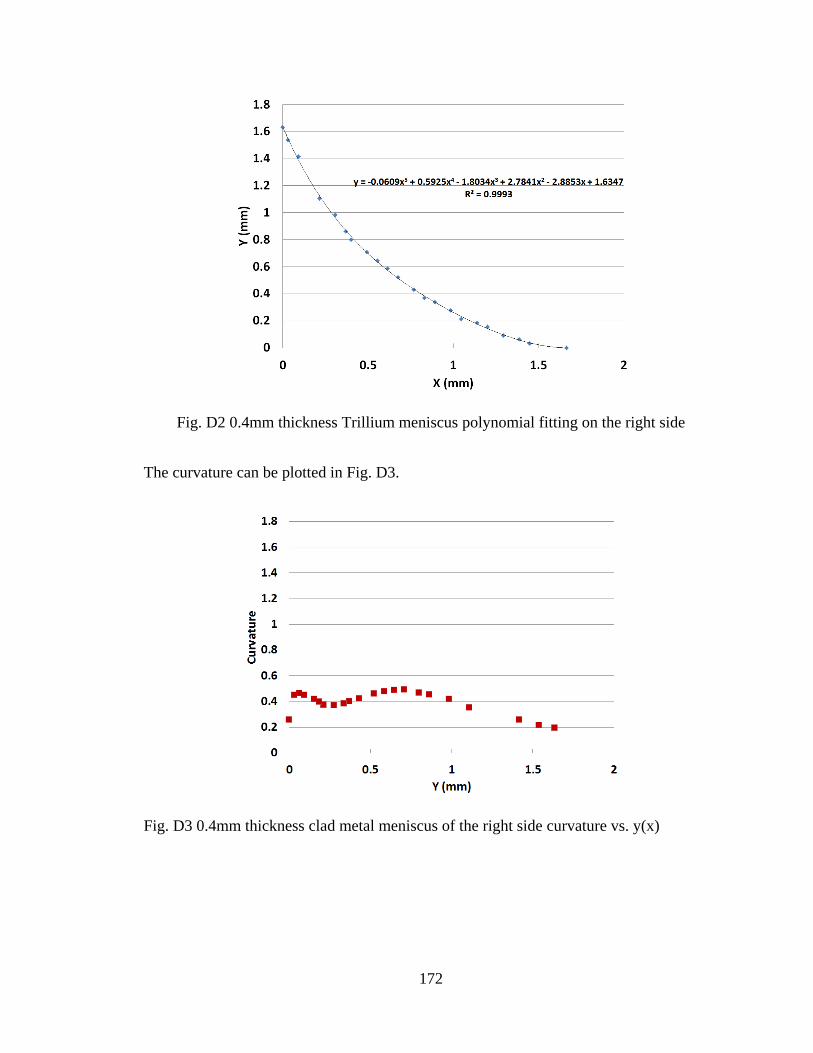
172
Fig. D2 0.4mm thickness Trillium meniscus polynomial fitting on the right side
The curvature can be plotted in Fig. D3.
Fig. D3 0.4mm thickness clad metal meniscus of the right side curvature vs. y(x)
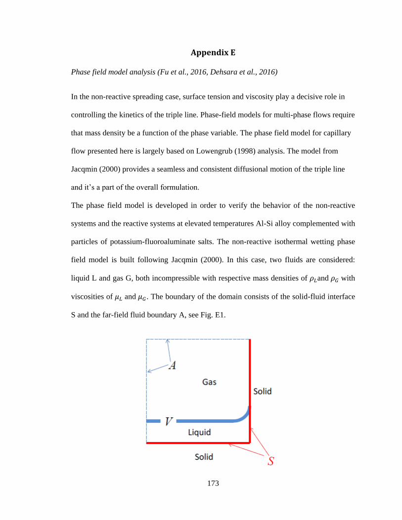
173
Appendix E
Phase field model analysis (Fu et al., 2016, Dehsara et al., 2016)
In the non-reactive spreading case, surface tension and viscosity play a decisive role in
controlling the kinetics of the triple line. Phase-field models for multi-phase flows require
that mass density be a function of the phase variable. The phase field model for capillary
flow presented here is largely based on Lowengrub (1998) analysis. The model from
Jacqmin (2000) provides a seamless and consistent diffusional motion of the triple line
and it’s a part of the overall formulation.
The phase field model is developed in order to verify the behavior of the non-reactive
systems and the reactive systems at elevated temperatures Al-Si alloy complemented with
particles of potassium-fluoroaluminate salts. The non-reactive isothermal wetting phase
field model is built following Jacqmin (2000). In this case, two fluids are considered:
liquid L and gas G, both incompressible with respective mass densities of 𝜌𝐿and 𝜌𝐺 with
viscosities of 𝜇𝐿 and 𝜇𝐺. The boundary of the domain consists of the solid-fluid interface
S and the far-field fluid boundary A, see Fig. E1.
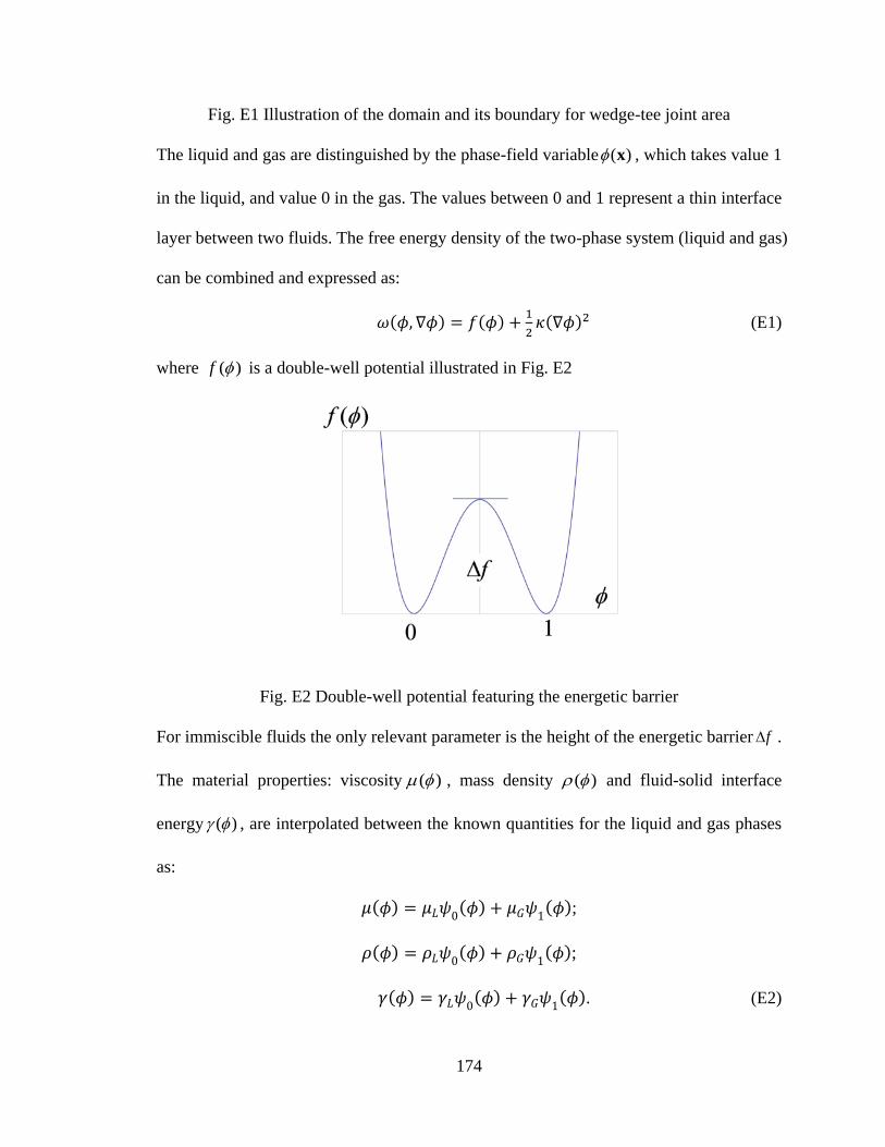
174
Fig. E1 Illustration of the domain and its boundary for wedge-tee joint area
The liquid and gas are distinguished by the phase-field variable ( ) x , which takes value 1
in the liquid, and value 0 in the gas. The values between 0 and 1 represent a thin interface
layer between two fluids. The free energy density of the two-phase system (liquid and gas)
can be combined and expressed as:
𝜔(𝜙, ∇𝜙) = 𝑓(𝜙) +1
2𝜅(∇𝜙)2 (E1)
where ( )f is a double-well potential illustrated in Fig. E2
Fig. E2 Double-well potential featuring the energetic barrier
For immiscible fluids the only relevant parameter is the height of the energetic barrier f .
The material properties: viscosity ( ) , mass density ( ) and fluid-solid interface
energy ( ) , are interpolated between the known quantities for the liquid and gas phases
as:
𝜇(𝜙) = 𝜇𝐿𝜓0(𝜙) + 𝜇𝐺𝜓
1(𝜙);
𝜌(𝜙) = 𝜌𝐿𝜓0(𝜙) + 𝜌𝐺𝜓
1(𝜙);
𝛾(𝜙) = 𝛾𝐿𝜓0(𝜙) + 𝛾𝐺𝜓
1(𝜙). (E2)
175
The interpolation functions must satisfy
𝜓0(𝜙) + 𝜓1(𝜙) = 1;𝜓0(𝜙 ≤ 0) = 0; 𝜓0(𝜙 ≥ 1) = 1 (E3)
The governing equations of the incompressible model consist of the modified Navier-
Stokes equations, the incompressibility condition and the 4th order Cahn-Hilliard
diffusion equation for the conserved phase field (Fu et al., 2016) as:
𝜌𝐷𝐯
𝐷𝑡= 𝜌𝐠 + ∇ ∙ [𝜇(𝐯∇ + ∇𝐯)] − ∇𝜋 + 𝑀∇𝜙; ∇ ∙ 𝐯 = 0;
𝐷𝜙
𝐷𝑡= 𝐵∇2𝑀; 𝑀 =
𝑑𝑓
𝑑𝜙− 𝜅∇2𝜙. (E4)
where ( )v x is velocity, ( ) x is incomplete pressure (including capillary and non-capillary
portions), B is the interface mobility, ( ) x is the phase field, D Dt is the material
derivative, g is the gravitational acceleration, and the dyadic 𝐯∇ is a rank-2 tensor with
components (𝐯∇)𝑖𝑗 = 𝜕𝑣𝑖 𝜕𝑥𝑗⁄ . The total pressure can be computed as:
𝑝 = 𝜋 − 𝑓 −1
6𝜅(∇𝜙)2 (E5)
The parameters and f are computed from the interface energy between the fluids
and the chosen width of the fluid-fluid interface (phase-field transition) h :
𝜅 =3
2ℎ, Δ𝑓 =
3
4 ℎ⁄ , (E6)
where ℎ is chosen to be much smaller than the smallest expected radius of curvature of
the fluid-fluid interface. In simulations, interface mobility B range should be first defined,
so that the results are insensitive to the order-of-magnitude changes in B. The capillary
stress tensor field is as follows:
𝛔 = (𝜔 − 𝑀𝜙)𝚰 − 𝜅∇𝜙∇𝜙, (E7)
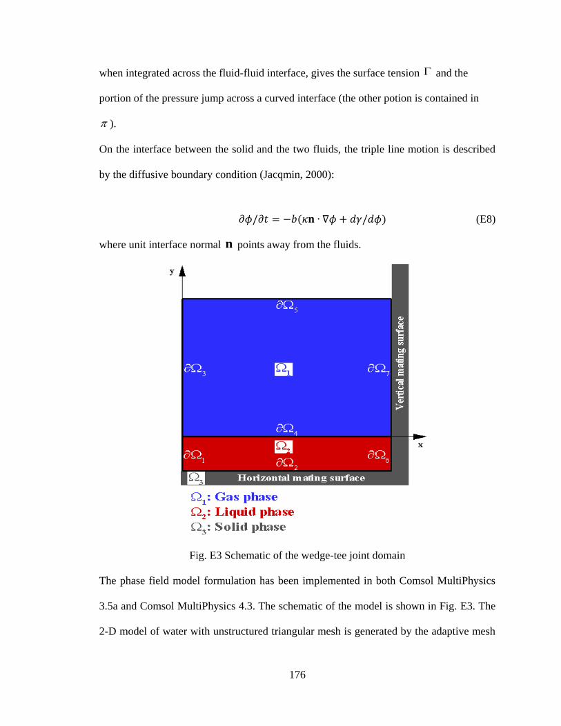
176
when integrated across the fluid-fluid interface, gives the surface tension and the
portion of the pressure jump across a curved interface (the other potion is contained in
).
On the interface between the solid and the two fluids, the triple line motion is described
by the diffusive boundary condition (Jacqmin, 2000):
𝜕𝜙/𝜕𝑡 = −𝑏(𝜅𝐧 ∙ ∇𝜙 + 𝑑𝛾/𝑑𝜙) (E8)
where unit interface normal n points away from the fluids.
Fig. E3 Schematic of the wedge-tee joint domain
The phase field model formulation has been implemented in both Comsol MultiPhysics
3.5a and Comsol MultiPhysics 4.3. The schematic of the model is shown in Fig. E3. The
2-D model of water with unstructured triangular mesh is generated by the adaptive mesh
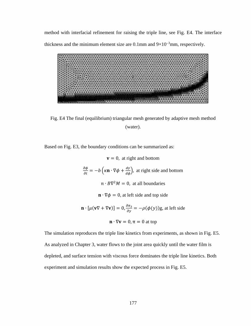
177
method with interfacial refinement for raising the triple line, see Fig. E4. The interface
thickness and the minimum element size are 0.1mm and 9×103mm, respectively.
Fig. E4 The final (equilibrium) triangular mesh generated by adaptive mesh method
(water).
Based on Fig. E3, the boundary conditions can be summarized as:
𝐯 = 0, at right and bottom
𝜕𝜙
𝜕𝑡= −𝑏 (𝜅𝐧 ∙ ∇𝜙 +
𝑑𝛾
𝑑𝜙), at right side and bottom
𝑛 ∙ 𝐵∇2𝑀 = 0, at all boundaries
𝐧 ∙ ∇𝜙 = 0, at left side and top side
𝐧 ∙ [𝜇(𝐯∇ + ∇𝐯)] = 0,𝜕𝜋3
𝜕𝑦= −𝜌(𝜙(𝑦))g, at left side
𝐧 ∙ ∇𝐯 = 0, π = 0 at top
The simulation reproduces the triple line kinetics from experiments, as shown in Fig. E5.
As analyzed in Chapter 3, water flows to the joint area quickly until the water film is
depleted, and surface tension with viscous force dominates the triple line kinetics. Both
experiment and simulation results show the expected process in Fig. E5.
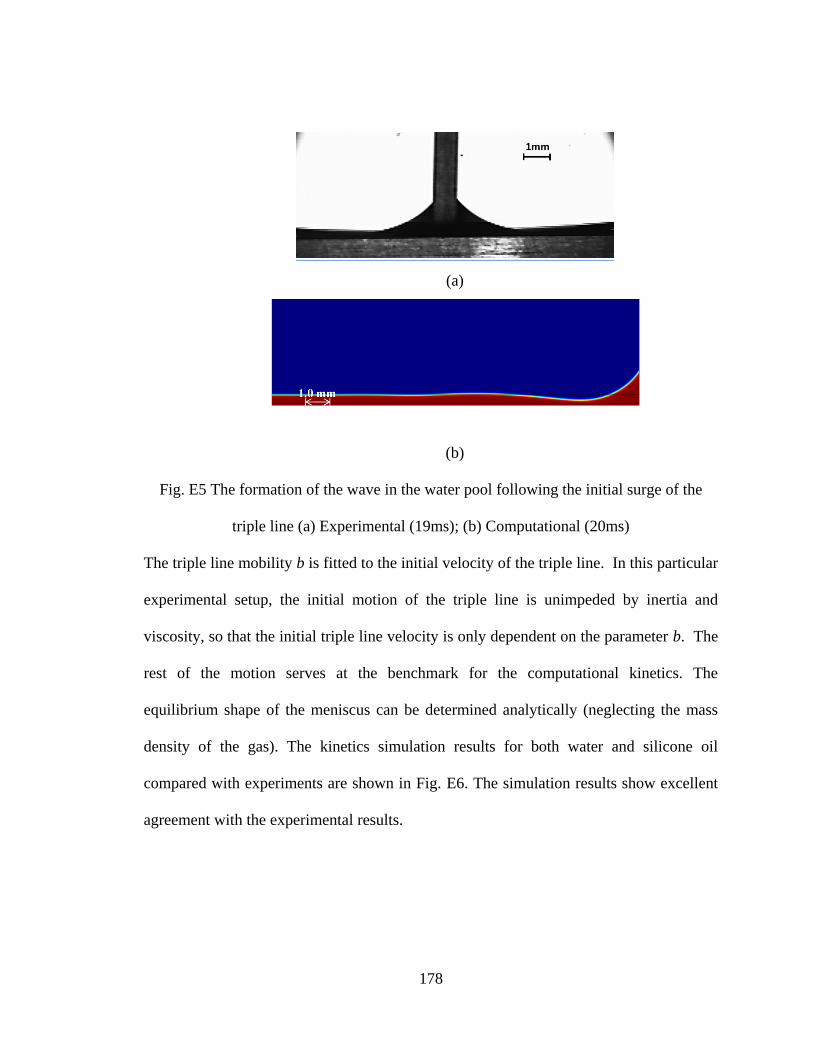
178
(a)
(b)
Fig. E5 The formation of the wave in the water pool following the initial surge of the
triple line (a) Experimental (19ms); (b) Computational (20ms)
The triple line mobility b is fitted to the initial velocity of the triple line. In this particular
experimental setup, the initial motion of the triple line is unimpeded by inertia and
viscosity, so that the initial triple line velocity is only dependent on the parameter b. The
rest of the motion serves at the benchmark for the computational kinetics. The
equilibrium shape of the meniscus can be determined analytically (neglecting the mass
density of the gas). The kinetics simulation results for both water and silicone oil
compared with experiments are shown in Fig. E6. The simulation results show excellent
agreement with the experimental results.
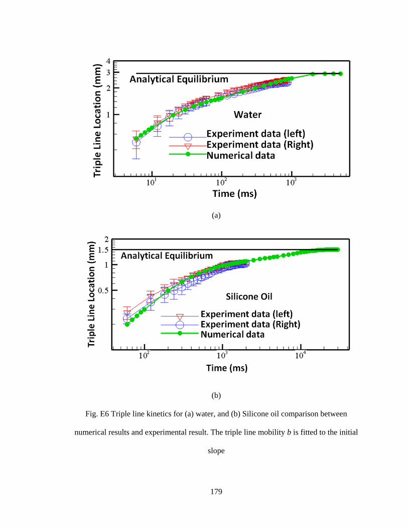
179
(a)
(b)
Fig. E6 Triple line kinetics for (a) water, and (b) Silicone oil comparison between
numerical results and experimental result. The triple line mobility b is fitted to the initial
slope
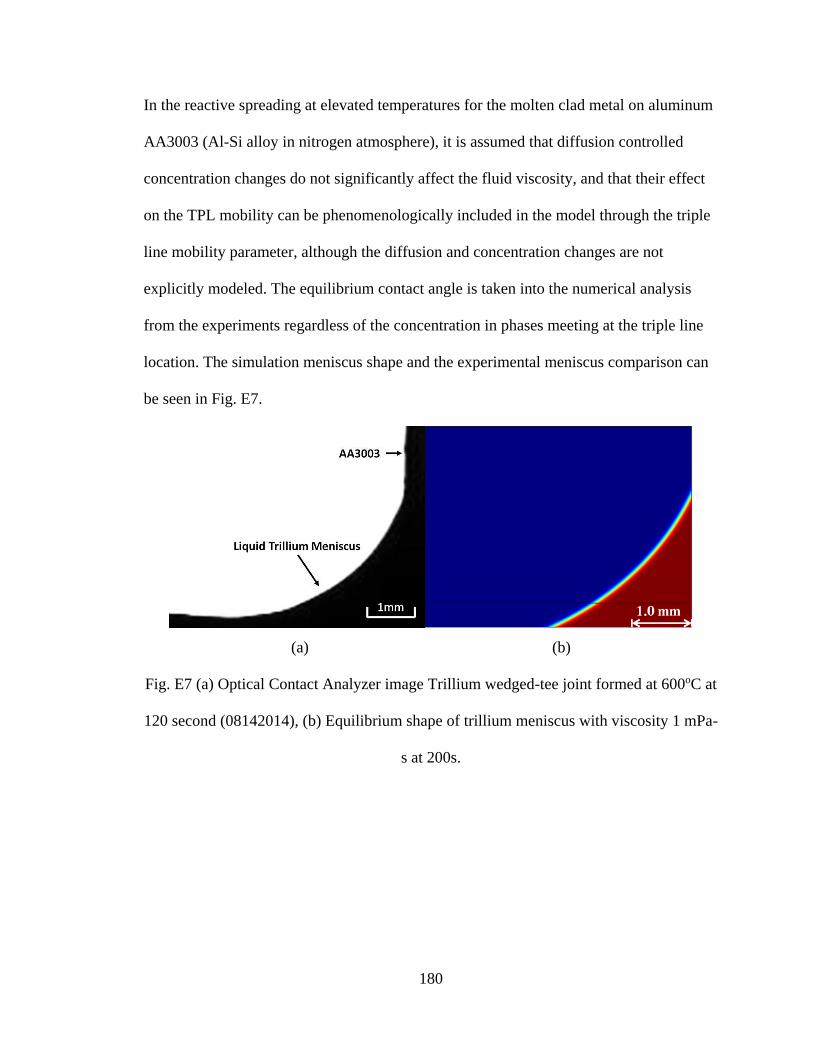
180
In the reactive spreading at elevated temperatures for the molten clad metal on aluminum
AA3003 (Al-Si alloy in nitrogen atmosphere), it is assumed that diffusion controlled
concentration changes do not significantly affect the fluid viscosity, and that their effect
on the TPL mobility can be phenomenologically included in the model through the triple
line mobility parameter, although the diffusion and concentration changes are not
explicitly modeled. The equilibrium contact angle is taken into the numerical analysis
from the experiments regardless of the concentration in phases meeting at the triple line
location. The simulation meniscus shape and the experimental meniscus comparison can
be seen in Fig. E7.
(a) (b)
Fig. E7 (a) Optical Contact Analyzer image Trillium wedged-tee joint formed at 600oC at
120 second (08142014), (b) Equilibrium shape of trillium meniscus with viscosity 1 mPa-
s at 200s.
181
REFERENCES
De Gennes, P.-G. (1985). "Wetting: statics and dynamics." Reviews of Modern
Physics 57(3): 827
Voinov, O. (1976). "Hydrodynamics of wetting." Fluid Dynamics 11(5): 714-721.
Dussan, E. (1979). "On the spreading of liquids on solid surfaces: static and dynamic
contact lines." Annual Review of Fluid Mechanics 11(1): 371-400.
Kistler, S. (1993). "Hydrodynamics of wetting." Wettability 6: 311-430.
Eustathopoulos, N., et al. (1999). Wettability at high temperatures, Elsevier.
Quéré, D. (2008). "Wetting and roughness." Annu. Rev. Mater. Res. 38: 71-99.
Bonn, D., et al. (2009). "Wetting and spreading." Reviews of Modern Physics 81(2):
739.
Sui, Y., et al. (2014). "Numerical simulations of flows with moving contact lines."
Annual Review of Fluid Mechanics 46: 97-119.
Sekulic, D. P. (2011). "Wetting and spreading of liquid metals through open
microgrooves and surface alterations." Heat Transfer Engineering 32(7-8): 648-657.
Zhao, H. and D. Sekulic (2006). "Diffusion-controlled melting and re-solidification
of metal micro layers on a reactive substrate." Heat and Mass Transfer 42(6): 464-
469.
Busbaher, D., et al. (2010). P1–26: High temperature brazing using nano-
particles doped filler metal for dispenser cathode applications. Vacuum Electronics
Conference (IVEC), 2010 IEEE International.
Schwartz, M. M. (2003). Brazing, ASM international.
Ogilvy, A. J. W., Hawkswoth, D. K., Abom, E., "Brazing piece, a method of making
a brazing piece, and a method of brazing and components made from said brazing
piece." U.S. Patent No. 8,871,356. 28 Oct. 2014.
Yu, C.-N., et al. (2013). An Analysis of an Impact of the Background Atmosphere
on the Aluminum Brazing Joint Formation. ASME 2013 International Mechanical
Engineering Congress and Exposition, American Society of Mechanical Engineers.
182
Hawksworth, D. K. (2012). Clad Melting and Joint Formation in Aluminum Brazing
Under Severe Alterations of the Background Atmosphere: A Superior New Brazing
Sheet Material Vs. a Traditional Brazing Sheet. 5th International Brazing and
Soldering Conference, Asm.
Sekulić, D. P. (2013). Advances in brazing: science, technology and applications,
Elsevier.
Fu, H., Dong, F., Sekulic, D. P., Mesarovic, S. D., & Krivilyov, M. (2013). Surface
Tension Driven Kinetics of the Triple Line of a Liquid Metal Free Surface.
In ASME 2013 International Mechanical Engineering Congress and Exposition , San
Diego, USA
Myers, D. (1999). "Wetting and spreading." Surfaces, Interfaces, and Colloids:
Principles and Applications, Second Edition: 415-447.
De Gennes, P.-G., et al. (2013). Capillarity and wetting phenomena: drops, bubbles,
pearls, waves, Springer Science & Business Media.
Yuan, Y. and T. R. Lee (2013). Contact angle and wetting properties. Surface
science techniques, Springer: 3-34.
Blake, T. and J. Haynes (1973). "Contact-angle hysteresis." Progress in surface and
membrane science 6: 125-138.
Rillaerts, E. and P. Joos (1980). "The dynamic contact angle." Chemical Engineering
Science 35(4): 883-887.
Johnson Jr, R. E., et al. (1977). "Dynamic contact angles and contact angle
hysteresis." Journal of Colloid and Interface Science 62(2): 205-212.
Seebergh, J. E. and J. C. Berg (1992). "Dynamic wetting in the low capillary number
regime." Chemical Engineering Science 47(17): 4455-4464.
Joanny, J. and P.-G. De Gennes (1984). "A model for contact angle hysteresis." The
Journal of Chemical Physics 81(1): 552-562.
Eral, H. and J. Oh (2013). "Contact angle hysteresis: a review of fundamentals and
applications." Colloid and polymer science 291(2): 247-260.
Young, T. (1805). "An essay on the cohesion of fluids." Philosophical Transactions
of the Royal Society of London: 65-87.
183
Washburn, E. W. (1921). "The Dynamics of Capillary Flow." Physical Review 17(3):
273-283.
Han, J. and C. Kim (2014). "Theoretical and experimental studies on the contact line
motion of second-order fluid." Rheologica Acta 53(1): 55-66.
Šikalo, Š., et al. (2005). "Dynamic contact angle of spreading droplets: Experiments
and simulations." Physics of Fluids (1994-present) 17(6): -.
Ström, G., et al. (1990). "Kinetics of steady-state wetting." Journal of Colloid and
Interface Science 134(1): 107-116.
Hocking, L. and A. Rivers (1982). "The spreading of a drop by capillary action."
Journal of Fluid Mechanics 121: 425-442.
Schwartz, A. M. and S. B. Tejada (1972). "Studies of dynamic contact angles on
solids." Journal of Colloid and Interface Science 38(2): 359-375.
Fermigier, M. and P. Jenffer (1991). "An experimental investigation of the dynamic
contact angle in liquid-liquid systems." Journal of Colloid and Interface Science
146(1): 226-241.
Sobolev, V., et al. (2000). "Surface tension and dynamic contact angle of water in
thin quartz capillaries." Journal of Colloid and Interface Science 222(1): 51-54.
Biance, A.-L., et al. (2004). "First steps in the spreading of a liquid droplet."
Physical Review E 69(1): 016301.
Lee, J. B. and S. H. Lee (2011). "Dynamic wetting and spreading characteristics of a
liquid droplet impinging on hydrophobic textured surfaces." Langmuir 27(11): 6565-
6573.
Calvo, A., et al. (1991). "Dynamic capillary pressure variations in diphasic flows
through glass capillaries." Journal of Colloid and Interface Science 141(2): 384-394.
Stokes, J., et al. (1990). "Harmonic generation as a probe of dissipation at a moving
contact line." Physical Review Letters 65(15): 1885.
Wilhelmy, L. (1863). "Ueber die Abhängigkeit der Capillaritäts‐Constanten des
Alkohols von Substanz und Gestalt des benetzten festen Körpers." Annalen der
Physik 195(6): 177-217.
Cain, J., et al. (1983). "Dynamic contact angles on smooth and rough surfaces."
Journal of Colloid and Interface Science 94(1): 123-130.
184
Bracke, M., et al. (1989). The kinetics of wetting: the dynamic contact angle. Trends
in Colloid and Interface Science III, Springer: 142-149.
Adam, N. K. and G. Jessop (1925). "CCL.—Angles of contact and polarity of solid
surfaces." Journal of the Chemical Society, Transactions 127: 1863-1868.
Fowkes, F. M. and W. D. Harkins (1940). "The state of monolayers adsorbed at the
interface solid—aqueous solution." Journal of the American Chemical Society
62(12): 3377-3386.
Smedley, G. T. and D. E. Coles (2005). "A refractive tilting-plate technique for
measurement of dynamic contact angles." Journal of Colloid and Interface Science
286(1): 310-318.
Vagharchakian, L., et al. (2008). "Capillary Bridge Formation and Breakage: A Test
to Characterize Antiadhesive Surfaces†." The Journal of Physical Chemistry B
113(12): 3769-3775.
Restagno, F., et al. (2009). "Contact angle and contact angle hysteresis
measurements using the capillary bridge technique." Langmuir 25(18): 11188-11196.
Hoffman, R. L. (1975). "A study of the advancing interface. I. Interface shape in
liquid—gas systems." Journal of Colloid and Interface Science 50(2): 228-241.
Voinov, O. (1976). "Hydrodynamics of wetting." Fluid Dynamics 11(5): 714-721.
Tanner, L. (1979). "The spreading of silicone oil drops on horizontal surfaces."
Journal of Physics D: Applied Physics 12(9): 1473.
Schwartz, A. M., & Tejada, S. B. (1970). NASA Contract Rep.
Jiang, T.-S., et al. (1979). "Correlation for dynamic contact angle." Journal of
Colloid and Interface Science 69(1): 74-77.
Blake, T., et al. (1995). "Models of wetting: Immiscible lattice Boltzmann automata
versus molecular kinetic theory." Langmuir 11(11): 4588-4592.
Meier, A., et al. (1999). "Ceramic-metal interfaces and the spreading of reactive
liquids." JOM 51(2): 44-47.
Saiz, E. and A. P. Tomsia (1998). "Kinetics of Metal‐Ceramic Composite Formation
by Reactive Penetration of Silicates with Molten Aluminum." Journal of the
American Ceramic Society 81(9): 2381-2393.
185
Contreras, A., et al. (2003). "Wettability and spreading kinetics of Al and Mg on
TiC." Scripta Materialia 48(12): 1625-1630.
Meier, A., et al. (1998). "Modelling of the spreading kinetics of reactive brazing
alloys on ceramic substrates: copper–titanium alloys on polycrystalline alumina."
Acta Materialia 46(12): 4453-4467.
Rado, C., et al. (2000). "The role of compound formation in reactive wetting: the
Cu/SiC system." Acta Materialia 48(18): 4483-4491.
Mortensen, A., et al. (1997). "Kinetics of diffusion-limited spreading of sessile drops
in reactive wetting." Scripta Materialia 36(6): 645-651.
Bailey, G. and H. Watkins (1951). "The flow of liquid metals on solid metal surfaces
and its relation to soldering, brazing, and hot-dip coating." Journal of the Institute of
Metals 80(2): 57-76.
Li, J. (1992). "Kinetics of wetting and spreading of Cu-Ti alloys on alumina and
glassy carbon substrates." Journal of Materials Science Letters 11(23): 1551-1554.
Dezellus, O., et al. (2002). "Chemical reaction-limited spreading: the triple line
velocity versus contact angle relation." Acta Materialia 50(19): 4741-4753.
Zhao, H. (2005). Transport Phenomena Involving Molten Clad During Aluminum
Brazing Process, University of Kentucky.
Thorsen, K. A., et al. (1984). "Optical hot stage microscopy for brazing
investigations." WELD J 63(11): 393.
Fujii, H., et al. (1993). "Interfacial reaction wetting in the boron nitride/molten
aluminum system." Acta Metallurgica et Materialia 41(10): 2963-2971.
Weirauch, D. and W. Krafick (1990). "The effect of carbon on wetting of aluminum
oxide by aluminum." Metallurgical Transactions A 21(6): 1745-1751.
Hager, Willi H. (2012). "Wilfrid Noel Bond and the Bond number", Journal of
Hydraulic Research 50 (1): 3–9.
Bashforth, F. and J. C. Adams (1883). An attempt to test the theories of capillary
action: by comparing the theoretical and measured forms of drops of fluid,
University Press.
Fu H., Dehsara M., Krivilyov M., Sekulic D.P., Mesarovic S.Dj., “Kinetics of the
Molten Al-Si Triple Line Movement during a Brazed Joint Formation”, Journal of
186
Material Science, 2016, 51(4), 1798-1812.
Chappuis, J., et al. (1982). "Multiphase Science and Technology." Eds. GF Hewitt,
JM Delhaye, and N. Zuber, Hemisphere Publishing Corporation 1: 387.
Rivollet, I., et al. (1990). "Simultaneous measurement of contact angles and work of
adhesion in metal-ceramic systems by the immersion-emersion technique." Journal
of Materials Science 25(7): 3179-3185.
Liu, W. and D. P. Sekulic (2011). "Capillary driven molten metal flow over
topographically complex substrates." Langmuir 27(11): 6720-6730.
Zhao, H., et al. (2009). "Wetting Kinetics of Eutectic Lead and Lead-Free Solders:
Spreading over the Cu Surface." Journal of Electronic Materials 38(2): 284-291.
Yu, C.-N., et al. (2013). An Analysis of an Impact of the Background Atmosphere
on the Aluminum Brazing Joint Formation. ASME 2013 International Mechanical
Engineering Congress and Exposition, American Society of Mechanical Engineers.
Zhao, H., et al. (2006). Surface tension driven molten metal flow over flat and/or
grooved reactive surfaces during brazing and soldering. International Brazing and
Soldering Conference, JJ Stephens, and KS Weil, Materials Park, OH: ASM
International.
Wen, L., et al. (2012). "Preferential spreading of molten metal over an
anisotropically microstructured surface." EPL (Europhysics Letters) 97(4): 46003.
Saiz, E. and Tomsia, A.P. (2005). "Kinetics of high-temperature spreading." Current
Opinion in Solid State and Materials Science 9(4): 167-173.
Saiz, E., et al. (2007). "Nonreactive spreading at high temperature: Molten metals
and oxides on molybdenum." Physical Review E 76(4): 041602.
Benhassine, M., et al. (2009). "Nonreactive spreading at high-temperature revisited
for metal systems via molecular dynamics." Langmuir 25(19): 11450-11458.
Champion, J., Keene, B., Sillwood, J. (1969). "Wetting of aluminium oxide by
molten aluminium and other metals." Journal of Materials Science 4(1): 39-49.
Drevet, B. and N. Eustathopoulos (2012). "Wetting of ceramics by molten silicon
and silicon alloys: a review." Journal of Materials Science 47(24): 8247-8260.
Candan, E., et al. (2011). "Wettability of Aluminum–Magnesium Alloys on Silicon
Carbide Substrates." Journal of the American Ceramic Society 94(3): 867-874.
187
Dezellus, O. and N. Eustathopoulos (2010). "Fundamental issues of reactive wetting
by liquid metals." Journal of Materials Science 45(16): 4256-4264.
Mortensen, A., et al. (1997). "Kinetics of diffusion-limited spreading of sessile drops
in reactive wetting." Scripta Materialia 36(6): 645-651.
Warren, J. A., et al. (1998). "Modeling reactive wetting." Acta Materialia 46(9):
3247-3264.
Voytovych, R., et al. (2007). "Reactive vs non-reactive wetting of ZrB 2 by
azeotropic Au–Ni." Acta Materialia 55(18): 6316-6321.
Yin, L., et al. (2009). "Reactive wetting in metal–metal systems." Journal of Physics:
Condensed Matter 21(46): 464130.
Dezellus, O., et al. (2002). "Chemical reaction-limited spreading: the triple line
velocity versus contact angle relation." Acta Materialia 50(19): 4741-4753.
Calderon, N. R., et al. (2010). "Wetting dynamics versus interfacial reactivity of
AlSi alloys on carbon." Journal of Materials Science 45(8): 2150-2156.
Lee, J.-I., et al. (2003). "Reactive wetting between molten Sn-Bi and Ni substrate."
Journal of Electronic Materials 32(3): 117-122.
Neumann, A. W., and R. J. Good. "Thermodynamics of contact angles. I.
Heterogeneous solid surfaces." Journal of Colloid and Interface Science 38, no. 2
(1972): 341-358.
Song, X., Bian, X., Zhang, J., Zhang,J. (2009). "Temperature-dependent viscosities
of eutectic Al–Si alloys modified with Sr and P." Journal of Alloys and Compounds
479(1): 670-673.
Neumann, A. W., and R. J. Good. "Thermodynamics of contact angles. I.
Heterogeneous solid surfaces." Journal of Colloid and Interface Science 38, no. 2
(1972): 341-358.
Eustathopoulos, N., et al. (2005). "Measurement of contact angle and work of
adhesion at high temperature." Journal of Materials Science 40(9-10): 2271-2280.
Hawksworth D.K., Sekulic D.P., Yu C.-N., Fu H., Westergard R.G.J., “A
Mechanistic Study of Aluminium Controlled Atmosphere Brazing Processes”, (May
188
10-13, 2015) Vehicle Thermal Management Systems Conference and Exhibition-
VTMS 12, Nottingham, England
http://www.coorstek.com/markets/electronic_equipment/ceramic-substrates.php,
Contact: [email protected]
http://www.uky.edu/design/index.php/info/category/digital_fabrication/
Stalder, A. F., et al. (2010). "Low-bond axisymmetric drop shape analysis for surface
tension and contact angle measurements of sessile drops." Colloids and Surfaces A:
Physicochemical and Engineering Aspects 364(1–3): 72-81.
Drop Shape Analysis. http://bigwww.epfl.ch/demo/dropanalysis/
Anson, J. P., et al. (1999). "The surface tension of molten aluminum and Al-Si-Mg
alloy under vacuum and hydrogen atmospheres." Metallurgical and Materials
Transactions B 30(6): 1027-1032.
Dorsey, N. E. (1928). A new equation for the determination of surface tension from
the form of a sessile drop or bubble. J. Wash. Acad. Sci,18(19), 505-509.
T. Iida, R.I.L. Guthrie, The Physical Properties of Liquid metals, Oxford Science
Publications, Oxford, 1988.
J.F. Paddy. "Surface Tension. Part II. The Measurement of Surface Tension." In
Surface and Colloid Science. Vol.1. Editted by E. Matijevic. Wiley, New York, 1968.
Kwok, D. Y. and A. W. Neumann (2000). "Contact angle interpretation in terms of
solid surface tension." Colloids and Surfaces A: Physicochemical and Engineering
Aspects 161(1): 31-48.
Goicoechea, J., et al. (1992). "Surface tension of binary and ternary aluminium
alloys of the systems Al-Si-Mg and Al-Zn-Mg." Journal of Materials Science 27(19):
5247-5252.
Aqra, F. and A. Ayyad (2012). "Surface tension (γLV), surface energy (γSV) and
crystal-melt interfacial energy (γSL) of metals." Current Applied Physics 12(1): 31-
35.
Keene, B. J. (1993). "Review of data for the surface tension of pure metals."
International Materials Reviews 38(4): 157-192.
189
Sarou-Kanian, V., et al. (2003). "Surface Tension and Density of Oxygen-Free
Liquid Aluminum at High Temperature." International Journal of Thermophysics
24(1): 277-286.
Mills, K. C. and Y. C. Su (2006). "Review of surface tension data for metallic
elements and alloys: Part 1 Pure metals." International Materials Reviews 51(6):
329-351.
Skapski, A. S. (1956). "A theory of surface tension of solids—I application to
metals." Acta Metallurgica 4(6): 576-582.
Su, Y., et al. (2005). "A model to calculate surface tension of commercial alloys."
Journal of Materials Science 40(9-10): 2185-2190.
Naidich, Y. V., et al. (1998). "The wettability of silicon carbide by Au–Si alloys."
Materials Science and Engineering: A 245(2): 293-299.
Eustathopoulos, N., et al. (1974). "The wetting of carbon by aluminium and
aluminium alloys." Journal of Materials Science 9(8): 1233-1242.
Flint, O. (1965). "Surface tension of liquid metals." Journal of Nuclear Materials
16(3): 233-248.
Zhivov, I. V. G. "Determination of surface tension of molten aluminum, magnesium,
sodium, and potassium." Tr. Vses. alyumino-magn, in-ta 14 (1937): 99.
Martins, G. P., D. L. Olson, and G. R. Edwards. "Modeling of infiltration kinetics
for liquid metal processing of composites." Metallurgical and Materials Transactions
B 19.1 (1988): 95-101.
Utigard, T. and J. M. Toguri (1985). "Interfacial tension of aluminum in cryolite
melts." Metallurgical Transactions B 16(2): 333-338.
Alchagirov, B. B., et al. (2003). "The Surface Tension of Melts of Aluminum–
Indium Binary System." High Temperature 41(4)
Alonso, A., et al. (1993). "Evaluation of the wettability of liquid aluminum with
ceramic particulates (SiC, TiC, AI2O3) by means of pressure infiltration."
Metallurgical Transactions A 24(6): 1423-1432.
Hatch, John E. Aluminum: properties and physical metallurgy. Vol. 1. Asm
International, 1984.
190
T. Iida, R.I.L. Guthrie, The Physical Properties of Liquid metals, Oxford Science
Publications, Oxford, 1988.
Rhee, S. K. "Wetting of ceramics by liquid aluminum." Journal of the American
Ceramic Society 53.7 (1970): 386-389.
Hashim, J., et al. (2001). "The wettability of SiC particles by molten aluminium
alloy." Journal of Materials Processing Technology 119(1–3): 324-328.
Goumiri, L., et al. "Tensions superficielles d'alliages liquides binaires présentant un
caractère dimmiscibilité: Al-Pb, Al-Bi, Al-Sn et Zn-Bi." Surface Science 83.2 (1979):
471-486.
ES Levin, GD Ayushina, High Temp., 1968, vol. 6, p. 416
Andreas, J. M., E. A. Hauser, and W. B. Tucker. "BOUNDARY TENSION BY
PENDANT DROPS1." The Journal of Physical Chemistry 42.8 (1938): 1001-1019.
s. I. POPEL, V. N. KOZHURKOV, and A. A. ZHUKOV: Izv. Akad.Nauk SSSR,
Met., 1975, (5), 69.
Iida, T. and R. Guthrie (2009). "Performance of a Modified Skapski Model for the
Surface Tension of Liquid Metallic Elements at Their Melting-Point Temperatures."
Metallurgical and Materials Transactions B 40(6): 967-978.
Egry, I., et al. "Surface tension measurements of high temperature metallic
melts." TRANSACTIONS-JWRI 30.SPI (2001): 195-200.
Goumiri, L. and J. C. Joud (1982). "Auger electron spectroscopy study of
aluminium-tin liquid system." Acta Metallurgica 30(7): 1397-1405.
Pamies, The measurement of surface tension of liquid aluminum by means of the
maximum bubble pressure method: the effect of surface oxidation, 1984
Lu, H. M. and Q. Jiang (2005). "Surface Tension and Its Temperature Coefficient for
Liquid Metals." The Journal of Physical Chemistry B 109(32): 15463-15468.
Liu, W., Lu L., Li, Y., Cai, Y., Sekulic, D.P. (2012). Preferential spreading of
molten metal over an anisotropicallymicrostructured surface. EPL (Europhysics
Letters) 97(4): 46003.
Lowengrub, J, Truskinowsky, L. 1998 Quasi-incompressible Cahn-Hilliard fluids
and topological transition. Proc. R. Soc. Lond. A 454, 2617-2654.
191
Jacqmin, D. 2000 Contact-line dynamics of a diffuse fluid interface. J. Fluid Mech.
402, 57-88.
Gao, F., Zhao, H., Sekulic, D.P., Qian, Y., Waller, L., (2002), “Solid state Si
diffusion and joint formation involving aluminum brazing sheet”, Materials Science
and Engineering, A337: 228-235
192
VITA
Hai Fu
Education
MSME, 2008
Refrigeration and Cryogenics Engineering, Shanghai Jiao Tong University, Shanghai,
China
BSME, 2005
Refrigeration and Cryogenics Engineering, Southeast University, Nanjing, Jiangsu,
China
Research Experience
Research Assistant/Teaching Assistant (University of Kentucky, 2012-Present)
Research Assistant/Teaching Assistant (University of Cincinnati, 2009-2011)
Certification
Advanced-Level English Interpretation Accreditation of Shanghai HR Credentials
for Special Expertise, The Organization Department of the CPC Shanghai
Committee, The Shanghai Municipal Personnel Bureau, The Shanghai Education
Commission and The Shanghai Adult Education Commission. License Number:
D19739. 2007
Journal Publications
1. Fu H., Dehsara M., Krivilyov M., Sekulic D.P., Mesarovic S.Dj., “Kinetics of the
Molten Al-Si Triple Line Movement during a Brazed Joint Formation”, Journal of
Material Science, 2016, 51(4), 1798-1812.
2. Dehsara, M, Fu, H, Mesarovic, S Dj, Sekulic, DP & Krivilyov, Phase-field
models for capillary flows. Submitted, April 2016 to Journal of Computational
Physics
3. D. P. Sekulic, H. Fu, A. Rabinkin, D. Busbaher, E. Leone, T. Preuss,
“Microstructure Refining of a Mo-Ni Brazing Filler Metal by a SiC Nanoparticles
Doping”, Welding Journal, submitted, 2016
4. Sekulic, Dusan P., Rahul Nehete, Cheng-Nien Yu, and Hai Fu. "An energy
sustainability metric." Energy 74 (2014): 37-44.
5. Hai Fu, Jingyi Wu, Ru-zuo Wang, “Experimental Analysis on Heat and Power
Supply Performance of Movable Miniature CCHP System”, Energy Technology,
2008, Vol. 29(2), p79-82.
193
Conference Proceedings
1. Winter, M., Bickel, R., Sekulic, D., Koch, H., Fu, H., Butler, B. “Spectral,
Directional Emittance at Elevated Temperature for Various Materials”, AIAA
Science and Technology Forum and Exposition (SciTech 2016), accepted, 4-8,
Jan, 2016.
2. Dehsara M., Mesarovic S.Dj., Fu H., Sekulic D.P., Krivilyov M., “Kinetics of the
Molten Metal Triple Line Movement: Phase Field Models and Experiments”,
International Conference on High Temperature Capillarity HTC-2015, May 17-21,
2015, Bad-Herrenalb, Germany.
3. D.P. Sekulic, H. Fu, A. Rabinkin, D. Busbaher, E. Leone, and T. Preuss,
“Positive Changes in the Mocrostructure Morphology of the Mo-Ni Eutectiv
Brazing Filler Metal Caused by Additions of SiC Nano-Particle Powder”,
International Brazing and Soldering Conference 2015, AWS, ASM, Pap. 0477-
000059, Apri 19-22, 2015, Long Beach, USA
4. D.P. Sekulic, H. Fu, A. Rabinkin, D. Busbaher, E. Leone, and T. Preuss,
“Mechanical Properties of Mo Joints Brazed Using Mo-Ni Brazing Filler Metal
Powder Doped by SiC Nano-Particles”, International Brazing and Soldering
Conference 2015, AWS, ASM, Pap. 0477-000058, pp. 1-6, Apri 19-22, 2015,
Long Beach, USA
5. Hawksworth D.K., Sekulic D.P., Yu C.-N., Fu H., Westergard R.G.J., “A
Mechanistic Study of Aluminium Controlled Atmosphere Brazing Processes”,
Vehicle Thermal Management Systems Conference and Exhibition-VTMS 12,
May 10-13, 2015, Nottingham, England.
6. Fazleena Badurdeen, Dusan Sekulic, Robert Gregory, Adam Brown, Hai Fu,
“Developing and Teaching a Multidisciplinary Course in Systems Thinking for
Sustainability: Lessons Learned through Two Iterations”, “Best Paper Award”:
121st ASEE Annual Conference & Exposition, June 15-18, 2014, Indianapolis, IN,
USA
7. Hai Fu, Fangxiao Dong, D P. Sekulic, S. Dj. Mesarovic, M. Krivilyov, "Surface
Tension Driven Kinetics of the Triple Line of a Liquid Metal Free
Surface", IMECE2013-62945, ASME 2013 International Mechanical
Engineering Congress & Exposition, November 13-21, 2013, San Diego,
California, USA.
8. Rahul Nehete, Cheng-Nien Yu, Hai Fu, Dusan P. Sekulic, “Energy Resource Use:
Sustainability Metric of a Manufacturing Process”, 26th International Conference
on Efficiency, July 16-19, 2013, Guilin, China.
9. Fazleena Badurdeen, Robert Gregory, Gregory Luhan, Margaret Schroder, Dusan
Sekulic, Leslie Vincent, Adam Brown, Hai Fu, “Experiences from Developing
and Teaching a Multi-disciplinary Course”, Kentucky Innovations Conference,
May 16-17, 2013, Lexington, Kentucky, USA.
10. Badurdeen, F., A. Brown, R. Gregory, H. Fu, M. Schroeder, D. Sekulic, L.
Vincent, and G. A. Luhan. "Reframing Interdisciplinary Approaches to Systems
Thinking for Sustainability." In Proceedings of the International Symposium on
Sustainable Systems & Technologies. 2013.
11. Hai Fu, D P. Sekulic, Triple Line Kinetics of Liquid Metal Free Surface Poster,

194
Forum on Sustainable Manufacturing, August 9th, 2013, Lexington, Kentucky,
USA.
12. Sang Young Son, Jae Yong Lee, Hai Fu, Sushant Anand, Francisco Romay,
Aaron Collins, “Personal and Wearable Ultrafine Particle Counter”, AAAR 30th
Annual Conference, October 3-7, 2011, Orlando, Florida, USA.