1

KINETIC THEORY OF SUPERTHERMAL ELECTRON TRANSPORT G. V. Khazanov1 and M. W. Liemohn2

1Geophysical Institute and Department of Physics, University of Alaska Fairbanks

Mailing address: Geophysical Institute, P. O. Box 757320, Fairbanks, AK 99775-7320 USA

2Space Physics Research Laboratory and Department of Atmospheric, Oceanic, and Space Sciences, University of Michigan, Ann Arbor

Mailing address: University of Michigan, 2455 Hayward St., Ann Arbor, MI 48109-2143 USA

Running Header: KHAZANOV AND LIEMOHN: SUPERTHERMAL ELECTRON THEORY

2

ABSTRACT Recent progress in kinetic modeling of su-perthermal electrons is reviewed. A brief de-scription of superthermal electrons is presented, followed by a description of the relevant theory and numerics necessary to properly simulate fast electron flow in the coupled ionosphere-magnetosphere system. Results are summarized for several recently-developed models based on these methods. First is the quantification and explanation of features of the superthermal electron distribution function con-sistent with observations. The effects of super-thermal electrons on the thermal plasma, in particular electrodynamic and collisional coup-ling, is presented and discussed. The concept of plasmaspheric transparency for inter-hemispheric superthermal electron flows is pre-sented based on simulation results. An analysis and comparison of the distribution function for several superthermal electron source terms are shown. The expected interactions between this population and plasma waves are discussed throughout the presentation, and a brief over-view of the new relativistic electron extensions of these models is also given.

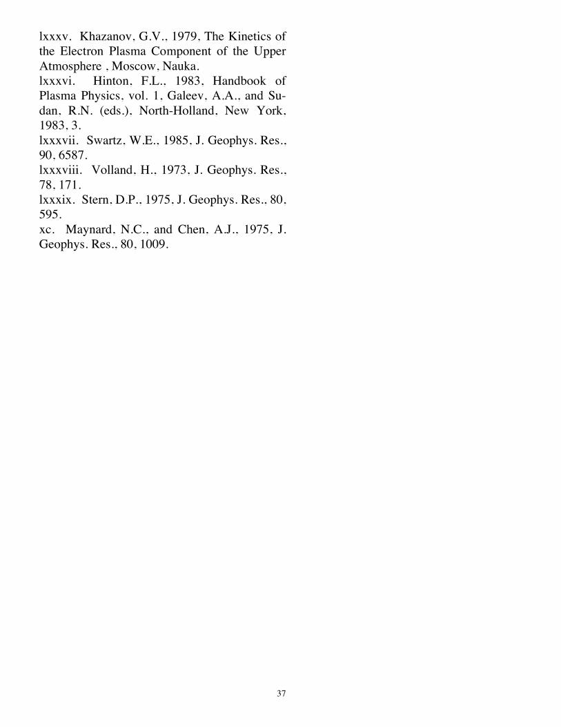
INTRODUCTION Two of the primary energy inputs into the ionosphere-magnetosphere system (see Figure 1 for a schematic view of near-Earth space) are energetic particles and extreme ultraviolet light, and one of the essential redistributors of energy from these sources is superthermal electrons. When an energetic particle or photon strikes an atmospheric neutral particle, an electron can be dislodged (processes known as impact ioniza-tion and photoionization, respectively). Due to the mass ratio of the dislodged electron to the ion, a large portion of the excess energy (that energy not used by ionization and possibly excitation) is carried away by the newly-freed electron. These electrons are known as super-thermal electrons, having energies (1-500 eV)

FIGURE 1 CALLOUT

3

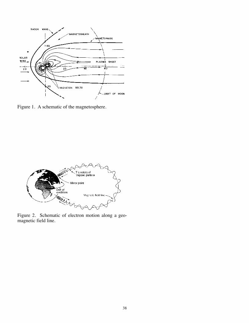
well above the thermal plasma temperature (≤1 eV), and a non-Maxwellian, anisotropic velo-city distribution. They are fast enough to escape from the ionosphere and move through the geomagnetic field to the conjugate ionosphere (see Figure 2 for a schematic of interhemispheric electron transport). As they travel, they not only are focused and defocused due to the inhomogeneous geomagnetic field, but also encounter many different phenomena and interact with them, including atmospheric neutral particles, thermal plasma particles, hot plasma particles, and plasma waves. Super-thermal electrons can gain or lose energy from any of these interactions, further changing the distribution function. Along the way, they lose energy through thermal plasma heating, ioni-zation and excitation of neutral particles, and generation of plasma waves. Furthermore, they also contribute to the formation of an ambipolar electric field along the magnetic field as they rapidly outpace the charge-neutralizing thermal ions. Superthermal electrons are ubiquitous throughout most of the ionosphere and magne-tosphere. Photoionization is dominant on the dayside, particularly in the low- to mid-latitude region, creating photoelectrons (PEs) in the ionosphere that can move into and fill the plasmasphere. Impact ionization dominates in the auroral and polar region, where primary particles (typically keV energy electrons) create secondary electrons in the superthermal energy range. Yet another non-collisional source is the acceleration of thermal plasma into this energy range. This happens in the equatorial plane of the magnetotail where turbulence and magneto-spheric convection energize the plasma popu-lation, creating plasma sheet electrons (PSEs). During times of active geomagnetic activity, PSEs are pushed into the inner magnetosphere to coexist with the PE population. They are also precipitated out of the magnetosphere down the flux tubes into the high-latitude iono-

FIGURE 2 CALLOUT

4

sphere, often undergoing field-aligned accel-eration that increases their speeds beyond the superthermal energy range (up to several keV) [e.g., 1]. These are the primary electrons re-sponsible for the impact ionization and secon-dary electron production (in the superthermal energy range) in this region. Modeling efforts to simulate the transport of superthermal electrons and their phase-space distribution function in the ionosphere have been conducted for several decades. They will be briefly mentioned here in order to put the present review into perspective. For a more detailed discussion of the history of superther-mal electron modeling, please see one of the several comprehensive reviews available in the literature [e.g., 2-4]. Many approaches have been used in these calculations, from local equilibrium approxima-tions [e.g., 5, 6] to particle-in-cell kinetic techniques [e.g., 7, 8] to direct solutions of the kinetic equation [e.g., 9-11]. It was known very early on that superthermal electrons could escape from their source regions and be trans-ported through the plasmasphere to the conju-gate ionosphere [12]. The first attempts at de-scribing this effect were qualitative in nature [13, 14], and more quantitative calculations of superthermal electron trapping in the plasma-sphere soon followed [15-19]. These calcula-tions presented the concept of plasmaspheric transparency, which is essentially a measure of the amount of flux that reaches the conjugate ionosphere. One of the problems with ionosphere-plas-masphere coupling is the vast timescale differ-ence between the two regions. A time-depend-ent model was developed that is equally valid in the ionosphere and plasmasphere [20], self-consistently coupling the two hemispheres. However, they simplified the equation by bounce-averaging the kinetic equation. A spa-tially self-consistent but time-independent cal-culation was also developed [2, 3].

5

A full realization of a time-dependent su-perthermal electron model that calculates the field-line profile of the distribution function was finally accomplished several years ago [21]. This model calculated non-steady-state superthermal electron transport in the plasmasphere (at altitudes greater than about 1000 km) based on the kinetic equation in the guiding center approximation. This model was expanded to include the ionospheric source re-gions [4, 22], including elastic and inelastic collisions with neutral particles, for a spatially self-consistent and time-dependent calculation along a flux tube. All of the above-mentioned studies dealt with a single flux tube of the geomagnetic field. One feature that is omitted from such an ap-proach is cross-field drifts. It was assumed that the flux tube was corotating with the Earth, so that cross field line drift effects could be ne-glected. A global scale model was developed [23] to examine the effects of convection of the superthermal electron distribution function. By averaging the distribution function along the field line (with appropriate mapping to con-serve the first adiabatic invariant), the high-en-ergy tail (E>50 eV) of the distribution was simulated throughout the inner magnetosphere. While other studies had investigated the flow of energetic electrons through near-Earth space [e.g., 24-26], this was the first to examine the time-dependent development of the PE distri-bution including cross-field convective drifts. This global model has also been used for the calculation of PSE entry into and motion through the inner magnetosphere. For instance, it was used to simulate PSE injection events and the creation of banded structures in the en-ergy spectrograms [27] that were seen in satel-lite measurements [28]. Further studies [29, 30] addressed the combination of the photoe-lectron and plasma sheet sources in the inner magnetosphere. The approach combined the global model [23] with the single tube model

6

[4] to create a fully three-dimensional calcula-tion of the superthermal electron distribution function for the entire energy range throughout the subauroral ionosphere and inner magneto-sphere. The present study reviews the theoretical and numerical concepts of the Khazanov and Liemohn superthermal electron kinetic trans-port models. It also presents a cogent summary of the research conducted thus far with the models, and gives a brief discussion of new di-rections being explored in electron transport modeling.

SUPERTHERMAL ELECTRON KINETIC THEORY

The theoretical basis of two non-steady-state models that have been recently developed to calculate the superthermal electron distribution function in the ionosphere-magnetosphere system [4, 23] will be described here. These two models complement each other and for the first time offer a unique possibility for simu-lating superthermal electron motion on a global scale. This discussion outlines the derivation of the equations solved in these models. Most space plasma modeling efforts begin their description of the particle motion with the Boltzmann kinetic equation,

!f

!t+

r v !f

!r x +

r a !f

!r v ="f

"t (1) which describes the evolution of the distribu-tion function, f, as a function of dependent vari-ables in the seven-dimensional phase space, f t,

r x ,

r v ( ). It includes changes in f due to time,

transport, internal and external acceleration mechanisms, sources, losses, and collisions. This equation, in this very general form, can be used to solve for the transport of anything, be it light through the atmosphere, particles through the magnetosphere, air over a wing, neutrons through graphite, water through the ground, or cars through city streets. However, it is not practical to use (1) for all of these flow proc-

7

esses. For some applications, it is not neces-sary to simulate all of the details of 7-dimen-sional phase space in order to get an accurate representation of the real flow patterns. That is, it is useful to limit the generality of (1) for the particular application to be addressed in order to gain computational speed without losing va-lidity of the result. Therefore, very few trans-port models actually solve (1). Most modeling efforts, in fact, make some reasonable assump-tions for the specific problem being investi-gated, and then solve this simplified transport equation. For superthermal electrons, the most obvious simplification is made by recognizing that the magnetic field dominates the motion of these particles. In a background magnetic field, charged particles gyrate about the magnetic lines of force, and the frequency of this gyra-tion, Ω=qB/m, is very fast for magnetospheric electrons (104 to 107 rad/sec). Therefore, the foremost reduction of (1) is to average over this gyrational motion. In this case, velocity space reduces to 2 variables, and instead of following the individual particles in configuration space, the equation solves for the motion of their gy-rational guiding center. Yet another simplifi-cation that is made possible by the magnetic dominance is that most spatial transport is along the magnetic field lines, and therefore cross-field drifts can be omitted in a first-order calculation. Under these assumptions, (1) can be rewritten as the field-aligned, guiding-center kinetic equation

!

E

"#

"t+ µ

"#

"s$1$ µ

2

2

1

B

"B

"s$

F

E

%

& '

(

) * "#

"µ

+ EFµ"#

"E= Q +

+#

+t (2) which calculates the time-dependent distribu-tion of the differential flux function, φ=2Ef/m2, as a function of time, distance along the field line, energy, and pitch angle. This is the equa-tion solved by our single flux tube model [4]

8

for superthermal electron transport in the Earth's ionosphere and plasmasphere. In (2), t is time; s is the distance along the field line; E is the particle energy; and µ is the cosine of the pitch angle (angle between the particle's helical motion and the magnetic field). The inhomo-geneity of the geomagnetic field, B, is included, as well as other forces, such as electric fields, in F. Q is the superthermal electron source term and δφ/δt includes the collision integrals, representing interactions with thermal electrons and ions, elastic and inelastic scattering with neutral particles, and wave-particle interactions, and is detailed in Appendix A. Terms of order me/mi and the second derivative with respect to energy will be omitted from the kinetic equa-tion calculations [3]. The model can be cou-pled with any neutral atmosphere model, ther-mal plasma model, and geomagnetic field model to calculate the electron flux along any magnetic field line for any set of background and initial conditions. From these results, the energy deposition to the thermal plasma and neutral atmosphere can be easily calculated, as well as the stability of the superthermal elec-tron distribution. A different approach to simplifying (1) is to recognize that the motion along the field line is quite fast compared to other timescales in the problem (for instance, collisional timescales). In this limit, it is possible to average the parti-cle fluxes along the field line over a magnetic mirror bounce period to eliminate the need for a field-aligned calculation. This bounce-averag-ing assumption is certainly true for the higher-energy superthermal electrons, those above a few tens of eV, and it was shown [29] that this assumption is also valid for the low-energy component of this population as long as it is not necessary to resolve the details of any transient field-aligned flow events. By including particle drifts across field lines, superthermal electron fluxes for the entire inner magnetosphere can

9

be determined by solving the bounce-averaged kinetic equation [23, 31]:

! f

!t+1

hµ0

!

!µ0

dµ0

dthµ

0f

"

# $

%

& '

+1

E

!

!E

dE

dtE f

"

# $

%

& '

+1

R2

!

!r R (

r V D R2 f( ) =

)f

)t CC

*fLC

0.5+ b (3)

where

r R ! includes the spatial directions per-

pendicular to the magnetic field, ! denotes averaging ξ over a bounce period along the field line, and h is a bounce-averaging factor. This is the equation solved by the second model of a superthermal electron transport [23], which calculates the distribution on a global scale. The right-hand side of (3) contains are collisional Coulomb interactions with the thermal plasma and atmospheric precipitation. The bounce-averaged drift and collision terms are detailed in Appendix B. The spatial extent of this model encircles the globe at radial dis-tances from L=1.75 out to L=6.5, providing a complementary solution of the kinetic equation to the first model throughout the subauroral magnetosphere. In fact, the two models were coupled [29, 30] to study the formation and evolution of the 3-dimensional total distribution function of superthermal electrons in near-Earth space. The combination of these models is possible because the formation of f within the loss cone (that is, those pitch angles that map to the ionosphere, where atmospheric losses generally absorb most of the superthermal electron energy) is much faster than the formation of f within the trapped zone (the larger pitch angles that do not map to the ionosphere). Therefore, (2) can be used for small pitch angles, calcu-lating the distribution along the field line and in both ionospheric endpoints, and (3) can be used for the larger pitch angles within the geomag-netic trap. At the interface, the results of (2)

10

are bounce-averaged and used as a boundary condition for (3), or vice versa, depending on the gradient of f at this pitch angle. It should be noted that both of these models are fully capable of including interactions with plasma waves [for a comprehensive review of magnetospheric plasma waves, see 32]. For example, one such interaction is with plasmas-pheric hiss. This radio-frequency wave is ex-cited in the plasmasphere, and is ubiquitous in the inner magnetosphere [33, 34]. Intense hiss is associated with density gradients [35-37], where the structures duct the waves into smaller wave normal angles, making them field-aligned (guided). The small wave normal angle permits these waves to resonate with lower energy electrons, down into the super-thermal energy range. Using quasilinear theory [38], diffusion timescales were calculated for plasmaspheric hiss interactions with superther-mal electrons [39]. They concluded that, for particular magnetospheric conditions, hiss could be a larger source of scattering than Coulomb collisions with the thermal plasma. These conditions are infrequent enough, how-ever, that plasma wave interactions will be omitted from the results to be presented below.

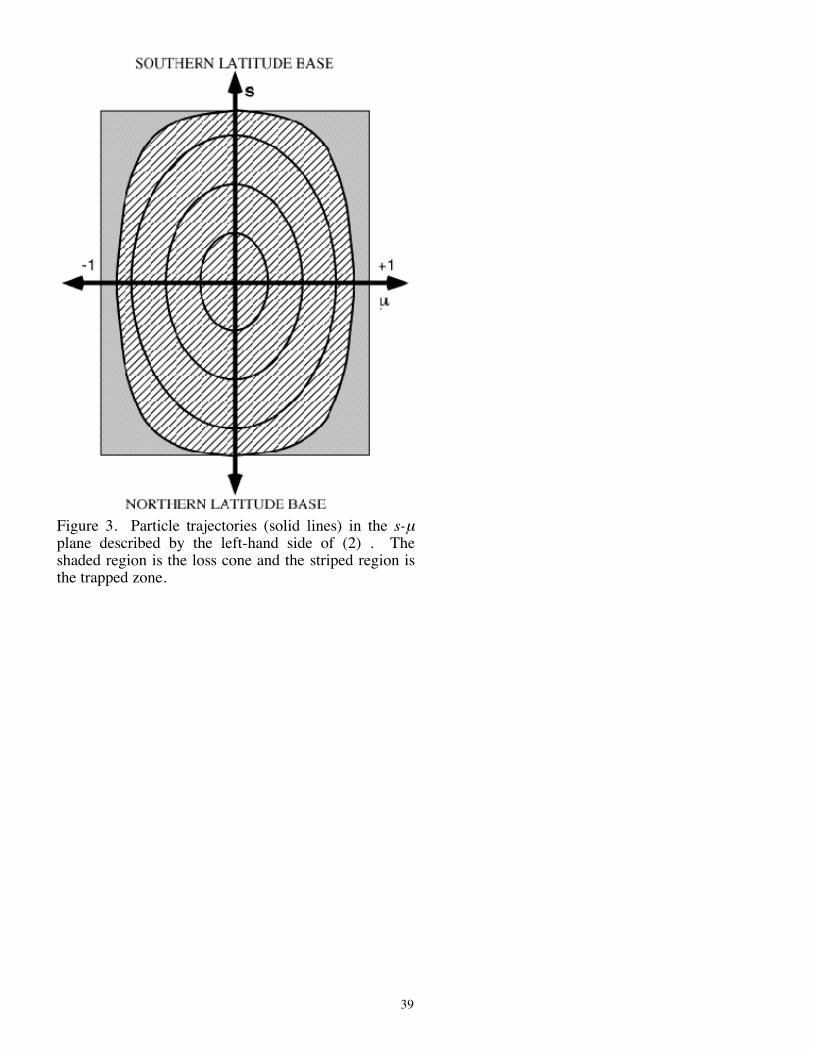
NUMERICAL IMPLEMENTATION As mentioned above, (2) is dominated by the motion along the field line (the ∂φ/∂s term). However, as the particle moves along the field line, its pitch angle is constantly changing be-cause of the nonuniform magnetic field (pitch angle decreases with B). This results in a regular oscillatory motion of the particles in s-µ space (see Figure 3) that can lead to serious numerical diffusion if the equation is solved on a Cartesian grid. Therefore, it is convenient to change variables to a set that will not contain this regular oscillatory motion. For the case without any field-aligned forces (F=0), the de-sired transformation is from s-E-µ to s-E-µ0. That is, the pitch angle variable is replaced by its equatorial value. In this case, (2) becomes

FIGURE 3 CALLOUT

11

!

E

" # $

"t+ µ

" # $

"s= # Q + # S (4)

where φ', Q' and ! S have been transformed to the new variables, and

µ0 s,µ( ) =µ

µ1!

B0

B s( )(1! µ

2) (5)

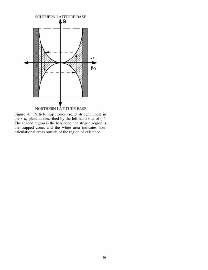
is an adiabatic invariant. In (5), B0 and µ0 de-note the magnetic field and the cosine of the pitch angle at the magnetic equator of the flux tube. The region over which φ(s, E, µ0) is de-fined in terms of s and µ0 is shown in Figure 4. The shaded region represents the loss cone, the striped region shows the trapped zone, and white indicates areas outside the region of ex-istence, where no calculation needs to occur. The loss cone is the set of pitch angles at a given altitude whose particles will not magneti-cally mirror before they reach ionospheric alti-tudes. It is defined by µob !µo !1 and the trapping region by 1!B0 B s( )( )

1 2

"µo "µob ,

where µob = 1!B0 B s1( )( )1 2

is the loss cone boundary and B s1( ) is the magnetic field at the chosen ionosphere-magnetosphere interface al-titude. The reflection point is determined as the location when µ(s,µ0)=0, that is, when B sref( )=B0 1!µ0

2( ) . Note that in these vari-ables, the set of derivatives on the left-hand side is reduced to time and space, and the only deviations from straight-line trajectories will be collisional processes, and thus numerical errors will be greatly reduced. Further details of this transformation are given elsewhere [40]. In the presence of a field-aligned force term, the desired variable transformation from s-E-µ to s-ε-µo to reduce numerical diffusion effects in the solution of (2) (that is, reduce (2) to (4) again). In this case, ε and µo are defined as ! s, E( ) = E " e#$ s( ) (6) and

FIGURE 4 CALLOUT

12

µos,E,µ( )=

µ

µ

! 1"BoE

B s( ) E"e #$ s( )"#$o( )[ ]1"µ 2( ) (7)

from the total energy of the particle and the first adiabatic invariant. In (6) and (7), ΔΦ(s) is the electrostatic potential difference along the field line, ΔΦ(s)=Φ(s)-Φ(sref), measured from an arbitrary reference point, sref. Also, ΔΦo is the potential difference between sref and so (the reference point for the constant term of the first adiabatic invariant). Further details of this transformation are also given elsewhere [41]. Using a developed set of boundary and initial conditions [4, 40], (4) can be solved for the new variable set with a generalized multi-stream approach taking into account energy degradation, pitch–angle focusing, pitch–angle diffusion, and field-aligned transport [40]. With the following finite-difference approximation for the derivatives,

!"

!t="n# "

n#1

$t (8a)

!"

!s=

"i# "

i #1

si# s

i#1

µ0

> 0

"i # "i +1

si# s

i+1

µ0 < 0

$

% & &

'

& &

(8b)

!"

!E=" j # " j +1

Ej# E

j+1

(8c)

where the subscripts n, i, and j are the time, space, and energy grid step indices, respectively, (4) is reduced to

A!2"

!µ0

2+ B

!2"

!µ0

+ C" = D (9)

Further difference replacements for the pitch angle derivatives of the form

13

!

!µ0=

"1

1" µ0

2

!

!# 0

! 2

!µ0

2=

1

1" µ0

2

! 2

!#0

2"

µ0

1" µ02( )

32

!

!#0

(10)

and

!"

!#0

=$1"k+1% $1+$2( )"k

$2$1+$

2( )+$1+$2( )"k%$2"k%1

$1$1+$

2( )

!2"

!#0

2=2$1"k+1%2 $1+$ 2( )"k +2$2"k%1

$1$2$1+$

2( ) (11)

where !1="0,k #"0,k#1 and ! 2 =" 0,k+1#"0,k , yields a tridiagonal matrix that is readily solved. At each energy step, the calculation is swept in both directions along the field line, solving (9) for each hemisphere of flow (µ0>0 and µ0<0), sharing information at the µ=0 boundary and iterating until the energy level has converged at all points in the s-µ0 plane. More details of this derivation can be found elsewhere [20, 21, 40]. To avoid large numer-ical diffusion and to obtain second-order accuracy in the time and space steps in (4), the two-step Lax-Wendroff method was used [42], which time (or space)-centers the integration by defining intermediate values of the dependent variables at the half time (space) steps tn+1/2 (s i+1/2 ). After each main step the intermediate values !i+1/2

n+1/2 are discarded and form no part of the solution [43] and thus were omitted in (8) for simplicity. In the second model, the numerical scheme used to solve (3) is a combination of advection schemes and diffusion techniques to obtain a second-order accurate result. However, it also must be transformed to take advantage of com-putational efficiencies. Namely, it must be converted to a conservative form of the kinetic equation where all of the advection coefficients are inside of the partial derivatives. In this case, the distribution function should be re-placed like this,

14

f =f*

R2 Ehµ0

(12)

and then (3) can be rewritten in conservative form,

! f *

!t+!

!r R "

r V D f

*( )+ !

!E

dE

dtf

*#

$ %

&

' (

+!

!µ0

dµ0

dtf *#

$ %

&

' ( =

)f *

)tCC

*f

LC

*

0.5+ b (13)

Note that the collisional terms also are con-verted to conservative form by this transforma-tion. The method of fractional steps [44] is used to separate (13) into a series of equations, setting each operator equal to the time deriva-tive operator. The azimuthal drift and energy loss terms are solved using a high-resolution method that combines the second-order Lax-Wendroff scheme with the first-order upwind scheme via a superbee flux limiter [45]. In this way, the limiter chooses the second-order scheme when the function is smooth, gradually converting to the first-order scheme near sharp gradients. Thus, it uses the numerical scheme most suited to the solution of the problem. A second-order accurate Crank-Nicolson scheme is used for the solution of the diffusion opera-tors [46]. Each of these equations is solved once, then again in reverse order to reduce systematic error and maintain second-order ac-curacy.

COMPARISONS OF SIMULATION RESULTS WITH OBSERVATIONS

These models have been used to address a number of issues regarding superthermal elec-tron transport and effects in the ionosphere-magnetosphere system. A summary of these results is presented to give the reader an indi-cation of the complexity of the superthermal electron distribution function, transport process, and energy deposition characteristics. This overview will begin with a comparison of model results against various direct and indirect

15

satellite measurements of superthermal elec-trons. To describe the basic features of the super-thermal electron distribution function, it is use-ful to present both simulation results and ob-servations. Since in situ measurements of su-perthermal electron distributions have primarily been conducted in the ionosphere (due to spacecraft charging effects contaminating su-perthermal electron observations in the mag-netosphere), we will limit our presentation to the three main spatial regions, according to the local transport characteristics: the collision-dominated region (below 200 km), the transi-tion region (up to ~1000 km), and the transport-dominated region (above 1000 km). The Atmospheric Explorer (AE) satellites offer a plentiful supply of superthermal electron energy spectra. The electron spectrometers on the AE satellites are ideal for comparison be-cause of the fine spectral resolution achieved in the low-energy range. Although the data is spin-averaged, this is not a big problem since the satellites flew through the low to middle ionosphere, where the distribution function is nearly isotropic. Figure 5 shows omnidirec-tional fluxes from the AE-E satellite and model results for similar conditions [47]. The data in this plot is for day 355 of 1975 at 182 and 365 km altitude [48]. This first altitude is in the re-gion where collisions with neutrals dominate the formation of the distribution function, and local production and loss mechanisms are the major processes in the calculation. The second altitude is in the transition region, where trans-port is starting to have a significant influence on the distribution. In Figure 5a, the spectra agree closely for most of the energy range, in-cluding definition in the 20-30 eV production peaks (peaks generated from the He-II 30.4 nm solar line ionizing the various constituents of the neutral atmosphere) and the N2 vibrational excitation bite-out in the distribution near 2 eV. The model predicts a slightly higher flux in the

FIGURE 5 CALLOUT

16

5-15 eV range, but this difference is less than a factor of two. Figure 5b also shows good agreement, with the model predicting more definition in the 20-30 eV range and lower fluxes above 30 eV by a factor of less than two. These differences could all be explained by un-certainties in the experimental data, differences in the neutral atmosphere or ionospheric plasma profiles, or uncertainties in the collisional cross sections used in the model. The larger fluxes at low energy and the increased definition of the production peaks in the model results indicate that the thermal plasma density from the International Reference Ionosphere (IRI) [49] used in the model is probably lower than the actual densities; a higher plasma density would act to smooth out these features of the distribution function. It is thought that this dif-ference is not due to detector resolution, be-cause ΔE/E was 2.5% and the production peaks clearly appear in the low altitude measure-ments. The comparison does show, however, that the model accurately calculates the main features of the photoelectron spectrum in the local equilibrium and transition regions of the ionosphere. It is interesting to note that the distribution of superthermal electrons is, in addition to being highly non-Maxwellian, quite spiky with many relative maxima. Such distributions can be un-stable to plasma wave excitation. In particular, a number of studies have examined the two main possibilities of wave growth in the iono-spheric photoelectron distribution: the decrease near 2-5 eV and the peaks near 20-30 eV, with much progress but no firm conclusion on the role of plasma instabilities. For example, sev-eral studies have claimed that the 2-5 eV region is unstable to wave growth [50-52] while sev-eral others claim that the distribution is stable in this energy range [53-55]. The stability of the 20-30 eV production peaks has also been extensively examined, again with some claim-ing it is an unstable energy range [56-58] and

17

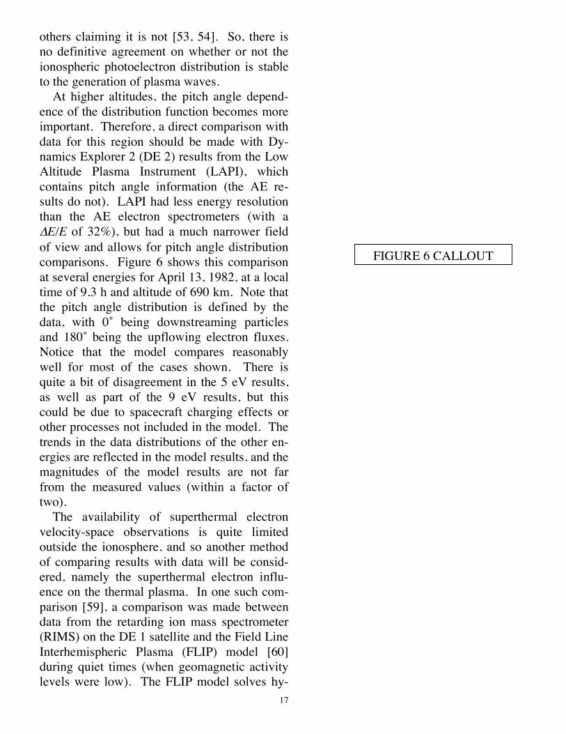
others claiming it is not [53, 54]. So, there is no definitive agreement on whether or not the ionospheric photoelectron distribution is stable to the generation of plasma waves. At higher altitudes, the pitch angle depend-ence of the distribution function becomes more important. Therefore, a direct comparison with data for this region should be made with Dy-namics Explorer 2 (DE 2) results from the Low Altitude Plasma Instrument (LAPI), which contains pitch angle information (the AE re-sults do not). LAPI had less energy resolution than the AE electron spectrometers (with a ΔE/E of 32%), but had a much narrower field of view and allows for pitch angle distribution comparisons. Figure 6 shows this comparison at several energies for April 13, 1982, at a local time of 9.3 h and altitude of 690 km. Note that the pitch angle distribution is defined by the data, with 0˚ being downstreaming particles and 180˚ being the upflowing electron fluxes. Notice that the model compares reasonably well for most of the cases shown. There is quite a bit of disagreement in the 5 eV results, as well as part of the 9 eV results, but this could be due to spacecraft charging effects or other processes not included in the model. The trends in the data distributions of the other en-ergies are reflected in the model results, and the magnitudes of the model results are not far from the measured values (within a factor of two). The availability of superthermal electron velocity-space observations is quite limited outside the ionosphere, and so another method of comparing results with data will be consid-ered, namely the superthermal electron influ-ence on the thermal plasma. In one such com-parison [59], a comparison was made between data from the retarding ion mass spectrometer (RIMS) on the DE 1 satellite and the Field Line Interhemispheric Plasma (FLIP) model [60] during quiet times (when geomagnetic activity levels were low). The FLIP model solves hy-

FIGURE 6 CALLOUT

18

drodynamic equations for the thermal plasma along a flux tube, combined with a superther-mal electron two-stream transport model (that is, only 2 pitch angle grid points, to resolve the upward and downward hemispherical fluxes) to calculate heating rates in the thermal plasma energy equations. This model includes a phe-nomenological factor (trapping factor) to repre-sent the amount of energy lost in the plasma-sphere by the photoelectrons. Without this trapping factor, the observed ion temperatures could not be reproduced, and it was concluded that good agreement is achieved between the calculated and measured ion temperatures when ~55% of the total photoelectron flux is trapped in the plasmasphere. A similar study was con-ducted with the field-line model [4], using the same thermal electron profile in the ionosphere and plasmasphere. They found that the portion of energy absorbed in the plasmasphere due to Coulomb losses with the thermal plasma is 0.53. This shows that our calculations are in agreement with phenomenological modeling and measurements of the thermal structure of the plasmasphere during quiet times. The accu-racy of the comparison also indicates that Coulomb interaction with the thermal plasma is the dominant process acting on the superther-mal electrons in the plasmasphere where the data was collected (midlatitudes on the day-side). SELF-CONSISTENT COUPLING WITH THE

THERMAL PLASMA The real power of the interhemispheric flux tube model is that it self-consistently calculates the time-dependence of the electron distribution in the ionosphere and plasmasphere. When coupled with a time-dependent thermal plasma model [e.g., 61], it also self-consistently calcu-lates the feedback between the thermal and su-perthermal plasma populations along a field line. Such a study was done for the case of plasmaspheric refilling [41], determining that photoelectrons can yield a large influence on

19

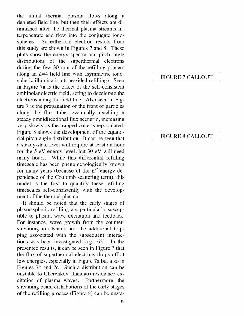
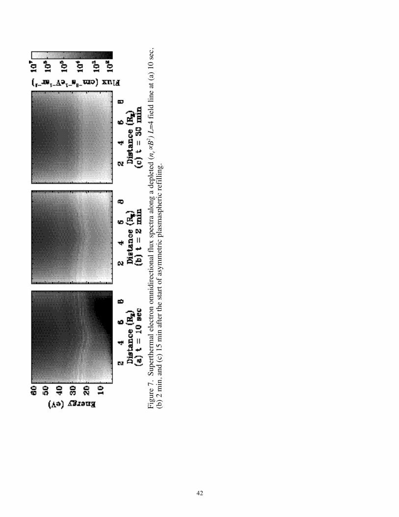
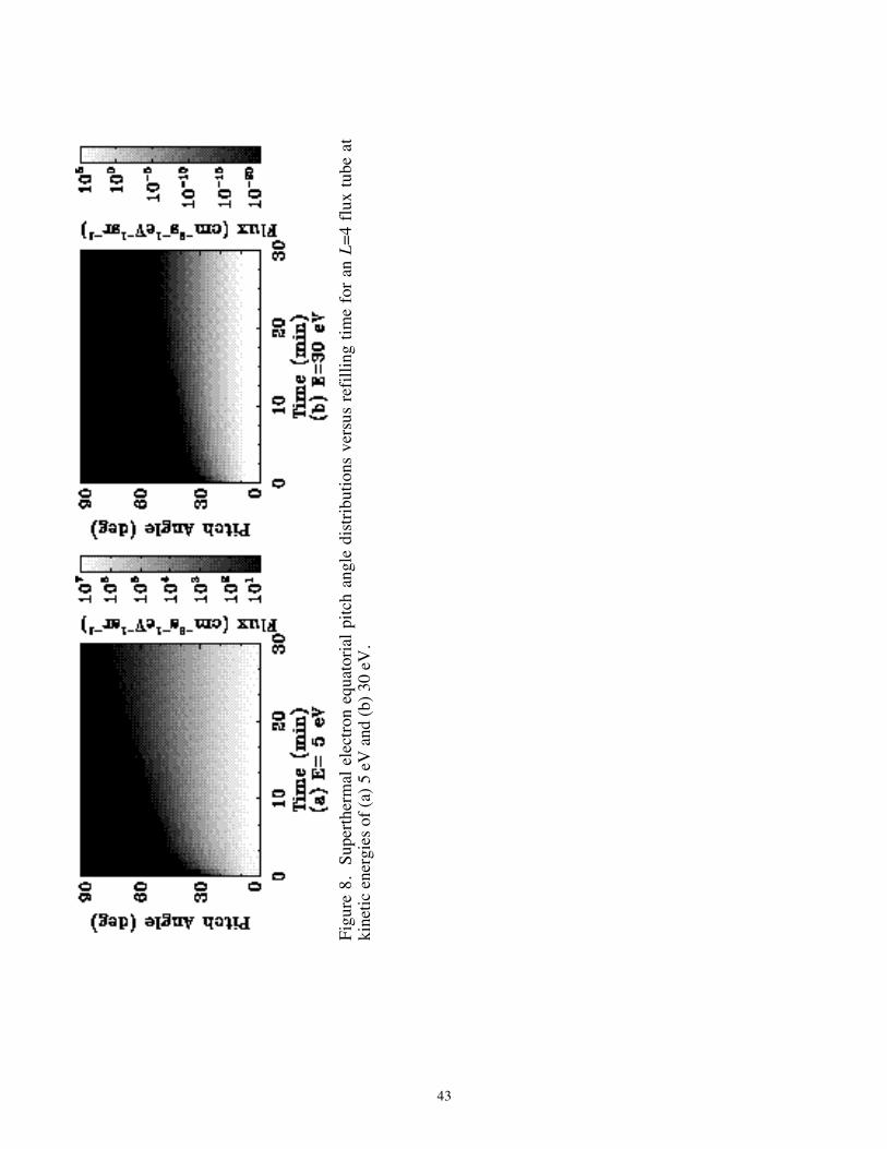
the initial thermal plasma flows along a depleted field line, but then their effects are di-minished after the thermal plasma streams in-terpenetrate and flow into the conjugate iono-spheres. Superthermal electron results from this study are shown in Figures 7 and 8. These plots show the energy spectra and pitch angle distributions of the superthermal electrons during the few 30 min of the refilling process along an L=4 field line with asymmetric iono-spheric illumination (one-sided refilling). Seen in Figure 7a is the effect of the self-consistent ambipolar electric field, acting to decelerate the electrons along the field line. Also seen in Fig-ure 7 is the propagation of the front of particles along the flux tube, eventually reaching a steady omnidirectional flux scenario, increasing very slowly as the trapped zone is repopulated. Figure 8 shows the development of the equato-rial pitch angle distribution. It can be seen that a steady-state level will require at least an hour for the 5 eV energy level, but 30 eV will need many hours. While this differential refilling timescale has been phenomenologically known for many years (because of the E-2 energy de-pendence of the Coulomb scattering term), this model is the first to quantify these refilling timescales self-consistently with the develop-ment of the thermal plasma. It should be noted that the early stages of plasmaspheric refilling are particularly suscep-tible to plasma wave excitation and feedback. For instance, wave growth from the counter-streaming ion beams and the additional trap-ping associated with the subsequent interac-tions was been investigated [e.g., 62]. In the presented results, it can be seen in Figure 7 that the flux of superthermal electrons drops off at low energies, especially in Figure 7a but also in Figures 7b and 7c. Such a distribution can be unstable to Cherenkov (Landau) resonance ex-citation of plasma waves. Furthermore, the streaming beam distributions of the early stages of the refilling process (Figure 8) can be unsta-

FIGURE 7 CALLOUT

FIGURE 8 CALLOUT

20

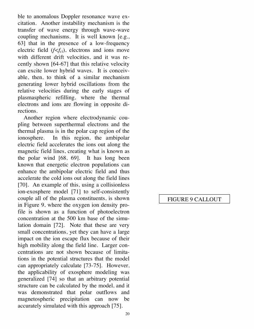
ble to anomalous Doppler resonance wave ex-citation. Another instability mechanism is the transfer of wave energy through wave-wave coupling mechanisms. It is well known [e.g., 63] that in the presence of a low-frequency electric field (f<fci), electrons and ions move with different drift velocities, and it was re-cently shown [64-67] that this relative velocity can excite lower hybrid waves. It is conceiv-able, then, to think of a similar mechanism generating lower hybrid oscillations from the relative velocities during the early stages of plasmaspheric refilling, where the thermal electrons and ions are flowing in opposite di-rections. Another region where electrodynamic cou-pling between superthermal electrons and the thermal plasma is in the polar cap region of the ionosphere. In this region, the ambipolar electric field accelerates the ions out along the magnetic field lines, creating what is known as the polar wind [68, 69]. It has long been known that energetic electron populations can enhance the ambipolar electric field and thus accelerate the cold ions out along the field lines [70]. An example of this, using a collisionless ion-exosphere model [71] to self-consistently couple all of the plasma constituents, is shown in Figure 9, where the oxygen ion density pro-file is shown as a function of photoelectron concentration at the 500 km base of the simu-lation domain [72]. Note that these are very small concentrations, yet they can have a large impact on the ion escape flux because of their high mobility along the field line. Larger con-centrations are not shown because of limita-tions in the potential structures that the model can appropriately calculate [73-75]. However, the applicability of exosphere modeling was generalized [74] so that an arbitrary potential structure can be calculated by the model, and it was demonstrated that polar outflows and magnetospheric precipitation can now be accurately simulated with this approach [75].

FIGURE 9 CALLOUT

21

PLASMASPHERIC TRANSPARENCY Another unique feature of this model is to set quantitative values to the concept of plasma-spheric transparency, T. This quantity is a measure of how easily the electrons fly through the plasmasphere to the conjugate ionosphere. Such a quantity is used by the numerous iono-sphere-only electron transport models (as de-scribed in the Introduction) to parameterize the plasmaspheric processes because these models assume a constant background magnetic field and are thus invalid in the magnetosphere. Using T, calculation in the conjugate iono-sphere can be conducted with a precipitating flux at the upper boundary from the interhemi-spheric transport of superthermal electrons. Historically, the value of T has been addressed qualitatively, but the flux tube model [4] can accurately define this parameter. Because of the energy dependence of the collisional times-cales for superthermal electrons, it is useful to describe transparency versus energy, T(E). There are several ways to define this quantity, so the first definition will be the ratio of parti-cle fluxes precipitating into one ionosphere di-vided by the particle fluxes flowing out of the conjugate ionosphere [16],

T E( )=

µ! s2,top ,E,µ( )dµ

0

1

"

µ! s1,top ,E,µ( )dµ0

1

" (14)

where s1,top is the location of the "top" of one ionosphere and s2,top is the altitude of the loca-tion of the "top" of the conjugate ionosphere. Note that this is not the probability of a single particle reaching the conjugate hemisphere, but rather is an attenuation factor such that the downward flux entering the conjugate iono-sphere is equal to the upward flux leaving the first ionosphere multiplied by T(E). Another definition for plasmaspheric transparency that could be used with ionospheric models is the ratio of the flux flowing down from the plasma-

22

sphere to the flux flowing up into the plasma-sphere,

T*E( )=

µ! s1,top,E,µ( )dµ"1

0

#

µ! s1,top,E,µ( )dµ0

1

# (15)

Notice that both integrals in (15) are at the same spatial location: the top of one of the ionospheres. T*(E) is an attenuation factor to obtain the flux entering an ionosphere given the flux leaving that same ionosphere. With this quantity, an ionospheric model can iterate to a solution in one ionosphere, without having to perform a calculation in the conjugate iono-sphere. Both of these quantities can be calculated with the interhemispheric model. Figure 10 shows two plasmaspheric transparencies for an L=2 field line. The results are for a "filled" flux tube, when the thermal plasma density along the field line can be assumed proportional to the magnetic field [59]. The solid line shows T(E) from (14) with both ionospheres illuminated (S. I. stands for "southern illumination"), while the dotted line shows T(E) with the southern hemisphere source term artificially omitted. There is a difference between these two results at low energies. The features of these curves are due to many things, including the features of the photoelectron production spectra of both ionospheres as well as the scattering processes included in the plasmasphere and both ionospheres. The transparency from (15) is also shown in Figure 10. The dashed line is T*(E) with south-ern hemisphere illumination, and the dash-dot-dot-dot line is T*(E) without this source in-cluded. There is quite a difference between these two lines. The only difference between T(E) and T*(E) with southern illumination is from differences in the photoelectron sources because of the dipole tilt. The difference be-

FIGURE 10 CALLOUT

23

tween these quantities without the southern source is drastic, particularly at high energies, because the numerator in (15) is produced only by backscattered electrons that started in the northern ionosphere. From these results, it can be concluded that the high-energy particles leaving the plasmasphere are primarily unhin-dered through the plasmasphere, with back-scattering occurring in the conjugate iono-sphere, while the low-energy electrons that leave the plasmasphere are mostly those back-scattered in the plasmasphere and not from the conjugate ionosphere. More details on plasma-spheric transparency are available elsewhere [4, 47].

GLOBAL TRANSPORT STUDIES The bounce-averaged superthermal electron transport model has also been used to answer unresolved questions of space physics. For in-stance, it was used to describe the cross-field drift effects on photoelectron distribution func-tion evolution [23], noting that convection not only built up extra flux in the afternoon sector but also carried photoelectrons, which only have a dayside source, around through the nightside in a narrow spatial band. It was also used to theoretically describe the banded structures in the energy spectrograms seen by the Combined Release and Radiation Effects Satellite (CRRES) in January 1991 [28], con-cluding that it was a natural consequence of the differential cross-field drift of electrons from the sub-keV to keV energy range [27]. Fur-thermore, it has been used in conjunction with the field line model to calculate the full 3-di-mensional distribution of superthermal elec-trons (from both photoelectrons and plasma sheet electrons) and its aeronomical effects [29, 30]. It is interesting to examine the combined distribution function in the superthermal energy range to understand how the bulk influences are generated. This will be done for the January 1991 results. Figure 11 shows energy spectra FIGURE 11 CALLOUT

24

for the two source populations at various spatial locations during the final Kp spike and PSE capture (late January 27, 1991). The spatial lo-cations are chosen to be in the nightside peak of the cloud (first row) and the nightside PE band (second band), and two analogous points on the dayside. Also, two equatorial pitch angles are shown: 90˚ and the loss cone boundary (LCB). Row 1 clearly shows the PSE dominance of the distribution throughout the pitch angle range, with fluxes several orders of magnitude larger than the PE fluxes at this location. In the nar-row PE band on the nightside, however, PEs dominate the low-energy range of the spectrum, even at 90˚. On the dayside, however, the in-tersection shifts to higher energies because of the proximity of the PE source, reaching 400 eV near the LCB at L=4. In every case, how-ever, the PSEs dominate the high-energy part of the spectrum, often with positive gradients in the distribution at the intersection and else-where. It can be seen that rotating the PSE re-sults by 12 hours will make the energy of the PSE-PE intersection decrease in the dayside plots, and will also make the PEs more compa-rable to the PSEs on the nightside. As time continues, the PSE fluxes will degrade (no more injections), allowing more of the PE dis-tribution to dominate the combined flux func-tion. The combined distribution function of su-perthermal electrons from these two sources is shown in Figure 12 throughout the CRRES ob-servations at the 4 spatial locations discussed in Figure 11 (again at 90˚ and the LCB). Here, the two populations have been summed into a single distribution. In the first column, PSEs form the nightside and PEs for the dayside dis-tributions, except for the high-energy bulge at 90˚ at L=6. After this, the distribution becomes mixed, except in the first row, which is always dominated by PSEs. The second row shows the PE distribution at low energies transitioning into the PSE distribution. The third column,

FIGURE 12 CALLOUT

25

however, shows no PE rise at low energies be-cause Kp remained sufficiently high to prevent them from reaching L=6 at midnight. The third and fourth rows also show the PEs at low ener-gies and the PSEs at high energies. There is a substantial number of spikes forming in the two L=4 rows at high energies. This is the banded structure forming inside of the Alfvén bound-ary after the capture of the PSEs, as the mag-netic drifts cause the electrons at these energies to have a drift period shorter than the corotation period, and they eventually lap the low-energy electrons. The spikes is not seen for most of the L=6 results because this is typically beyond the Alfvén boundary. Only after extended quiet times would this radial distance develop the banded structure seen closer in. Note that these spikes could be unstable to cyclotron or Landau resonance excitation of plasma waves. Addi-tionally, the large disparity between the trapped zone and the loss cone (the difference between the two curves in Figure 12) could also be unstable to wave growth. Another important result from this model output is the energy deposition to the thermal plasma. As the superthermal electrons convect through the inner magnetosphere, they interact with many things, including the background plasma. Because of the nature of the Coulomb force between charged particles, most of the energy transfer is from the superthermal elec-trons to the thermal electrons. Figure 13 shows heating rates from the combined source (PE and PSE) superthermal electrons into the ambi-ent thermal electrons. These values have been integrated along the field line and therefore are the heat fluxes into the topside ionosphere cor-responding to these equatorial plane locations. Two extreme cases are shown, one for quiet geomagnetic activity with a strong PE source and a weak PSE source, and another for active geomagnetic conditions with a weak PE source and a strong PSE source (note that weak and strong are relative terms, and that there is far

FIGURE 13 CALLOUT

26

more variability in the PSE source function than in the PE source). In the first case (top panel), it is clear that PEs dominate the super-thermal electron heating rates into the thermal electrons, and that the PSEs only contribute a minor amount of heat far out on the dawn side. In the second case (lower panel), the PSEs have encroached on most of the inner magnetosphere while the PE heating rates have diminished sig-nificantly on the dayside (however, they are still dominant there). A critical factor in cal-culating these heating rates is the distribution of thermal plasma, which for these cases was given by the chosen dynamic plasmasphere model [76]. When coupled with this thermal plasma model, the global model can predict the time-dependent heating rates into the thermal plasma throughout the inner-magnetospheric region, and can be used to identify the signifi-cance of energy deposition from superthermal electrons into the plasmasphere, topside iono-sphere, and thermosphere. This was the point of a particular study [30], where it was con-cluded that PEs dominate the dayside heating rates at all times, and that PSEs dominate the heating rates in the post-midnight sector during geomagnetic active times.

RELATIVISTIC BEAM MODELING An important advance in hot electron mod-eling is that both of the models discussed in this review have been extended to include the rela-tivistic energy range. In particular, these stud-ies have focused on simulating the evolution of a relativistic electron beam through the iono-sphere and magnetosphere. About 15 years ago, relativistic electron beam linear accelera-tors (LINACs) were reduced in size to the point where they could be feasibly flown onboard spacecraft, suborbital rockets, and balloons. While there has been some modeling efforts to describe the dynamics of these injected parti-cles [77-80], no study had examined the inter-hemispheric transport of these beams. How-ever, the flux tube model [4] was converted to

FIGURE 14 CALLOUT

27

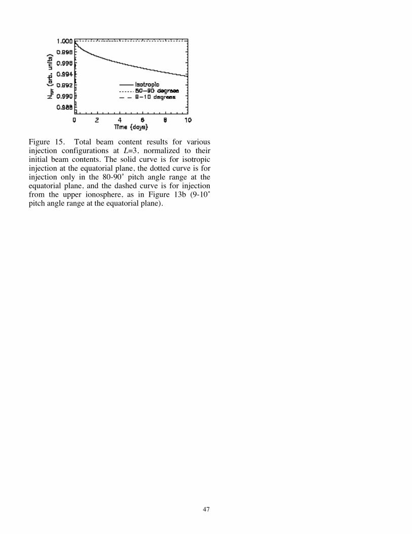
include relativistic effects and used to simulate the initial evolution of the beam [81], and the bounce-averaged model [23] was similarly converted and the global structure of the beam evolution was quantified [82]. While the entire phase-space distribution was calculated, of par-ticular interest is the lifetime of these particles in the inner magnetosphere. Figure 14 shows the normalized total particle count for various simulations conducted with the global model [82]. A notable finding of that study was that the injected beam transforms from a localized packet into a shell around the Earth. This shell initially forms within an hour of injection, but exhibits a banded energy spectrum structure for many hours, and does not become a uniform shell until perhaps a day after injection. All of these simulations, however, were for upper ionospheric injection (say, from the space shuttle). Figure 15 shows the normalized total particle count for several equatorial injec-tion simulations [83]. It is clear that the life-time can be strikingly different depending on the circumstances of the injection, and for some scenarios the beam can persist on timescales comparable to those of the natural radiation en-vironment [see, e.g., 84]. Therefore, while the studies thus far have focused on anthropogenic sources of relativistic electrons, these studies have particular relevance for radiation belt sci-ence. In fact, relativistic beam injections and the simulation of such experiments can be used as controlled tracer experiments to investigate the natural radiation environment.

DISCUSSION The time-dependent magnetospheric trans-port models for superthermal electrons de-scribed above offer the first opportunity to computationally quantify the evolution of this population's distribution function. This has al-lowed for the rigorous analysis of satellite measurements in order to place responsibility for certain features of the observations on spe-cific geophysical processes and phenomena.

FIGURE 15 CALLOUT

28

Take, for instance, plasmaspheric transparency. The attenuation factor has been known to exist for a long time, but only these models can accurately define the energy dependence of this quantity under realistic physical conditions. Furthermore, these are the only models that calculate the full 3-dimensional distribution function of hot electrons in near-Earth space. Much has been done over the years to under-stand the nature of superthermal electrons in the Earth's plasma environment. This review has attempted to present a summary of the his-tory of superthermal electron modeling in the terrestrial ionosphere and magnetosphere, and specifically to summarize the theory, numerical approach, and primary results from several re-cent studies of time-dependent superthermal electron transport modeling. It is the hope of the authors that this exposition will be a useful tool for the understanding of the state-of-the-art in this field.

APPENDIX A The collision term in (2) can be written as the sum of several distinction collision operators [85],

!"

!t=See+ Sei

0

i

# + Se$0

$# + Se$

*

$# + Se$

+

$# (A1)

The terms See , Sei0 , Se!

0 , Se!* , and Se!

+

represent the collision integrals of superthermal electrons with thermal electrons,

See =Ane

!

!E

"

E+Te

!

!E

"

E

# $ % &

' ( )

* + ,

- . / 0 1

+1

4E2

!

!µ12µ2( )!"

!µ

)

* + ,

- . 3 4 5

(A2)

with thermal ions,

Sei

0 = Ani

m

mi

!

!E

"

E+Ti

!

!E

"

E

# $ % &

' ( )

* + ,

- . / 0 1

+1

4E2

!

!µ12µ

2( )!"!µ

)

* + ,

- . 3 4 5

(A3)

elastic scattering with neutral particles,

29

Se!0 =2

m

m!

n!"

"E#!

(1) E2 $

E+Tn

"

"E

$

E

% & ' (

) * +

, - .

/ 0 1 2 3

4 5 6

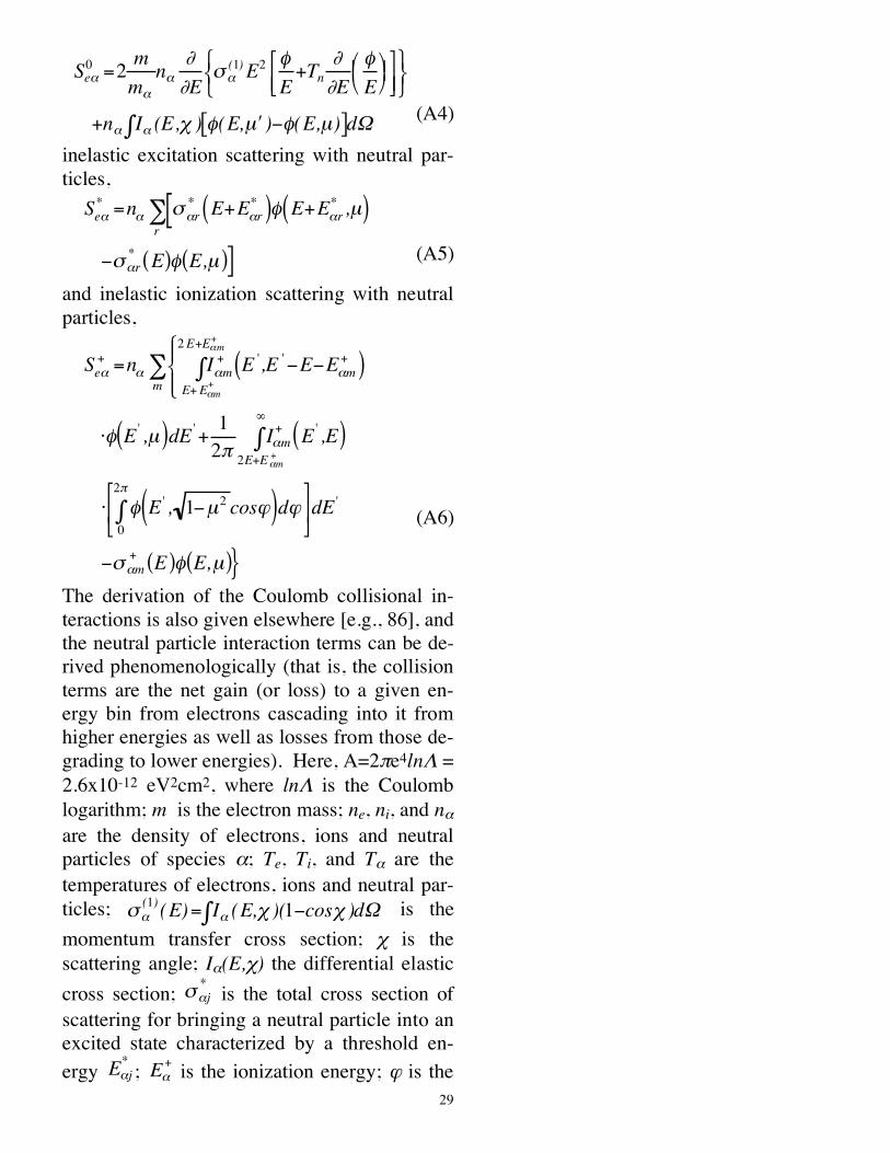
+n! I!7 (E,8 ) $(E, 9 µ ):$(E,µ)[ ]d; (A4)

inelastic excitation scattering with neutral par-ticles,

Se!* =n! "!r

*E+E!r

*( )# E+E!r

*,µ( )[

r

$

%"!r

*E( )# E,µ( )] (A5)

and inelastic ionization scattering with neutral particles,

Se!+ =n! I!m

+E

',E

'"E"E!m

+( )E+ E!m

+

2E+E!m+

#$ % &

' & m

(

)* E',µ( )dE

' +1

2+I!m

+E

',E( )

2E+E!m+

,

#

) * E', 1"µ2

cos-( )d-0

2+

#.

/ 0

1

2 3 dE

'

"4!m

+E( )* E,µ( )}

(A6)

The derivation of the Coulomb collisional in-teractions is also given elsewhere [e.g., 86], and the neutral particle interaction terms can be de-rived phenomenologically (that is, the collision terms are the net gain (or loss) to a given en-ergy bin from electrons cascading into it from higher energies as well as losses from those de-grading to lower energies). Here, A=2πe4lnΛ = 2.6x10-12 eV2cm2, where lnΛ is the Coulomb logarithm; m is the electron mass; ne, ni, and nα are the density of electrons, ions and neutral particles of species α; Te, Ti, and Tα are the temperatures of electrons, ions and neutral par-ticles; !"

(1)(E)= I"# (E,$ )(1%cos$ )d& is the

momentum transfer cross section; χ is the scattering angle; Iα(E,χ) the differential elastic cross section; !"j

* is the total cross section of scattering for bringing a neutral particle into an excited state characterized by a threshold en-ergy E!j

* ; E!+ is the ionization energy; ϕ is the

30

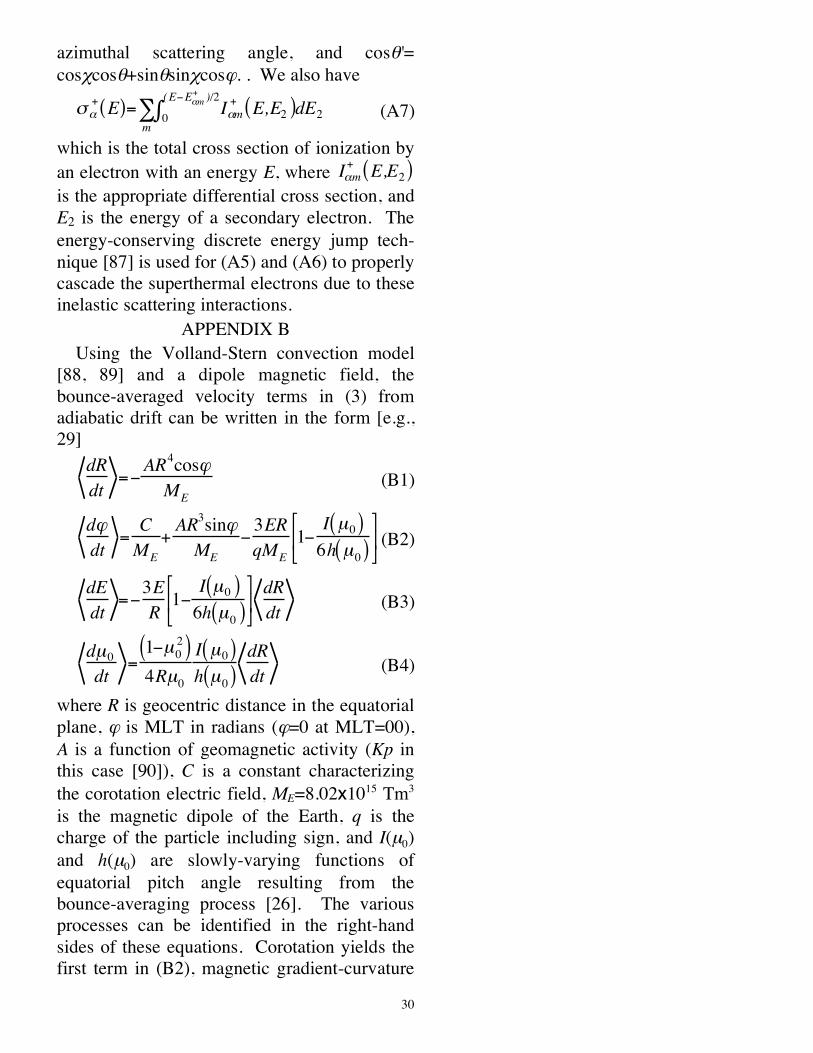
azimuthal scattering angle, and cosθ'= cosχcosθ+sinθsinχcosϕ. . We also have

!"+E( )= I"m

+

0

(E#E"m+)/2

$ E,E2( )dE2m

% (A7)

which is the total cross section of ionization by an electron with an energy E, where I!m

+E,E2( )

is the appropriate differential cross section, and E2 is the energy of a secondary electron. The energy-conserving discrete energy jump tech-nique [87] is used for (A5) and (A6) to properly cascade the superthermal electrons due to these inelastic scattering interactions.

APPENDIX B Using the Volland-Stern convection model [88, 89] and a dipole magnetic field, the bounce-averaged velocity terms in (3) from adiabatic drift can be written in the form [e.g., 29]

dR

dt=!

AR4cos"

ME

(B1)

d!

dt=C

ME

+AR

3sin!

ME

"3ER

qME

1"I µ0( )6h µ

0( )

#

$ %

&

' ( (B2)

dE

dt=!3E

R1!

I µ0( )6h µ

0( )

"

# $

%

& ' dR

dt (B3)

dµ0dt

=1!µ

0

2( )4Rµ

0

I µ0( )h µ

0( )dR

dt (B4)

where R is geocentric distance in the equatorial plane, ϕ is MLT in radians (ϕ=0 at MLT=00), A is a function of geomagnetic activity (Kp in this case [90]), C is a constant characterizing the corotation electric field, ME=8.02x1015 Tm3 is the magnetic dipole of the Earth, q is the charge of the particle including sign, and I(µ0) and h(µ0) are slowly-varying functions of equatorial pitch angle resulting from the bounce-averaging process [26]. The various processes can be identified in the right-hand sides of these equations. Corotation yields the first term in (B2), magnetic gradient-curvature

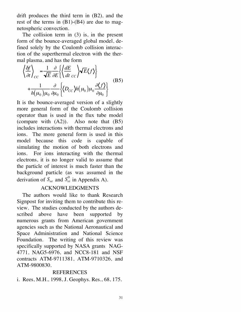
31

drift produces the third term in (B2), and the rest of the terms in (B1)-(B4) are due to mag-netospheric convection. The collision term in (3) is, in the present form of the bounce-averaged global model, de-fined solely by the Coulomb collision interac-tion of the superthermal electron with the ther-mal plasma, and has the form

!f

"t CC

=1

E

"

"E

dE

dt CC

E f# $ %

& ' (

+1

h µ0( )µ0

"

"µ0

DCC h µ0( )µ0

" f

"µ0

# $ %

& ' (

(B5)

It is the bounce-averaged version of a slightly more general form of the Coulomb collision operator than is used in the flux tube model (compare with (A2)). Also note that (B5) includes interactions with thermal electrons and ions. The more general form is used in this model because this code is capable of simulating the motion of both electrons and ions. For ions interacting with the thermal electrons, it is no longer valid to assume that the particle of interest is much faster than the background particle (as was assumed in the derivation of See and Sei

0 in Appendix A). ACKNOWLEDGMENTS

The authors would like to thank Research Signpost for inviting them to contribute this re-view. The studies conducted by the authors de-scribed above have been supported by numerous grants from American government agencies such as the National Aeronautical and Space Administration and National Science Foundation. The writing of this review was specifically supported by NASA grants NAG-4771, NAG5-6976, and NCC8-181 and NSF contracts ATM-9711381, ATM-9710326, and ATM-9800830.

REFERENCES i. Rees, M.H., 1998, J. Geophys. Res., 68, 175.

32

ii. Khazanov, G.V., Gombosi, T.I., Nagy, A.F., and Koen, M.A., 1992, J. Geophys. Res., 97, 16,887. iii. Khazanov, G.V., Neubert, T. and Gefan, G.D., 1994, IEEE Trans. Plasma Sci., 22, 187. iv. Khazanov, G.V., and Liemohn, M.W., 1995, J. Geophys. Res., 100, 9669. v. Hoegy, W.R., Fournier, J.-P., and Fontheim, E. G., 1965, J. Geophys. Res., 70, 5464. vi. Victor, G.A., Kirby-Docken, K., and Dal-garno, A., 1976, Planet. Space Sci., 24, 679. vii. Cicerone, R.J., and Bowhill, S.A., 1971, J. Geophys. Res., 76, 8299. viii. Papadopoulos, K., and Rowland, H.L., 1978, J. Geophys. Res., 83, 5768. ix. Banks, P.M., and Nagy, A.F., 1970, J. Geo-phys. Res., 75, 1902. x. Popov, G.V., and Khazanov, G.V., 1973, Studies in Geomagnetism, Aeonomy, and Solar Physics, vol. 27, Nauka, Moscow, 100. xi. Mantas, G.P., 1975, Planet. Space Sci., 23, 337. xii. Hanson, W.B., 1963, Space Res., 3, 282. xiii. Fontheim, E.G., Beutler, A.E., and Nagy, A.F., 1968, Ann. Geophys., 24, 489. xiv. Sanatani, S., and Hanson, W.B., 1970, J. Geophys. Res., 75, 769. xv. Gastman, I.J., 1973, Ph.D. thesis, Univ. of Mich., Ann Arbor. xvi. Takahashi, T., 1973, Rep. Ionos. and Space Res. Jap., 27, No. 1, 79. xvii. Lejeune, J., and Wörmser, F., 1976, J. Geophys. Res., 81, 2900. xviii. Khazanov, G.V., Koen, M.A. and Ba-raishhuk, S.I., 1977, Cosmic Res., 15, 68. xix. Krinberg, I.A., and Matafonov, G.K., 1978, Ann. Geophys., 34, 89. xx. Gefan, G.D., and Khazanov, G.V., 1990, Ann. Geophys. 8, 519. xxi. Khazanov, G.V., Liemohn, M.W., Gom-bosi, T.I., and Nagy, A.F., 1993, Geophys. Res. Lett., 20, 2821. xxii. Liemohn, M.W., and Khazanov, G.V., 1995, Cross-Scale Coupling in Space Plasmas,

33

Geophys. Monogr. Ser., vol. 93, Horwitz, J.L., Singh, N., and Burch, J.L. (eds.), AGU, Wash-ington, D. C., 185. xxiii. Khazanov, G.V., Moore, T.E., Liemohn, M.W., Jordanova, V.K., and Fok, M.-C., 1996, Geophys. Res. Lett., 23, 331. xxiv. Alfvén, H., and Fälthammar, C.-G., 1963, Cosmical Electrodynamics, Oxford Uni-versity Press, London. xxv. Roederer, J.G., 1970, Dynamics of Geo-magnetically Trapped Radiation, Springer-Verlag, New York. xxvi. Ejiri, M., 1978, J. Geophys. Res., 83, 4798. xxvii. Liemohn, M.W., Khazanov, G.V., and Kozyra, J.U., 1998, Geophys. Res. Lett., 25, 877. xxviii. Burke, W.J., Rubin, A.G., Hardy, D.A., and Holeman, E.G., 1995, J. Geophys. Res., 100, 7759. xxix. Khazanov, G.V., Liemohn, M.W., Kozyra, J.U., and Moore, T.E., 1998, J. Geo-phys. Res., 103, 23,485. xxx. Khazanov, G.V., Liemohn, M.W., and Kozyra, J.U., 2000, J. Atmos. Solar-Terr. Physics, in press. xxxi. Jordanova, V.K., Kistler, L.M., Kozyra, J.U., Khazanov, G.V., and Nagy, A.F., 1996, J. Geophys. Res., 101, 111. xxxii. Shawhan, S.D., 1979, Solar System Plasma Physics, vol. 3, Lanzerotti, L.J., Kennel, C.F., and Parker, E.H. (eds.), North-Holland, New York, 221. xxxiii. Thorne, R.M., Smith, E.J., Burton, R.K., and Holzer, R.E., 1973, J. Geophys. Res., 78, 1581. xxxiv. Smith, E.J., Frandsen, A.M., Tsurutani, B.T., Thorne, R.M., and Chan, K.-W., 1974, J. Geophys. Res., 73, 1. xxxv. Kozyra, J.U., et al., 1987, Adv. Space. Res., 7, 3. xxxvi. Hayakawa, M., Ohmi, N., Parrot, M., and Lefeuvre, F., 1986, J. Geophys. Res., 91, 135.

34

xxxvii. Hayakawa, M., Parrot, M., and Lefeu-vre, F., 1986, J. Geophys. Res., 91, 7989. xxxviii. Kennel, C.F., and Petschek, H.E., 1966, J. Geophys. Res., 71, 1. xxxix. Liemohn, M.W., Khazanov, G.V., and Kozyra, J.U., 1997, J. Geophys. Res., 102, 11,619. xl. Khazanov, G.V., Koen, M.A., and Bu-renkov, S.I., 1979, Cosmic Res., 17, 385. xli. Liemohn, M.W., Khazanov, G.V., Moore, T.E., and Guiter, S.M., 1997, J. Geophys. Res., 102, 7523. xlii. Lax, P.D., and Wendroff, B., 1960, Comm. Pure Appl. Math., 13, 217. xliii. Potter, D., 1973, Computational Physics, John Wiley & Sons, New York. xliv. Yanenko, N.N., 1971, The Method of Fractional Steps: The Solution of Problems of Mathematical Physics in Several Variables, Springer-Verlag, New York. xlv. Leveque, R.J., 1992, Numerical Methods for Conservation Laws, 2nd ed., Birkhäuser Verlag, Boston. xlvi. Anderson, D.A., Tannehill, J.C., and Pletcher, R.H., 1984, Computational Fluid Me-chanics and Heat Transfer, Hemisphere, Washington, D. C. xlvii. Khazanov, G.V., and Liemohn, M.W., 1998, Geospace Mass and Energy Flow, Geo-phys. Monogr. Ser., vol. 104, Horwitz, J.L., Gallagher, D.L., and Peterson, W.K. (eds.), AGU, Washington, D. C., 333. xlviii. Doering, J.P., Peterson, W.K., Bostrom, C.O., and Potemra, T.A., 1976, Geophys. Res. Lett., 3, 129. xlix. Bilitza, D., 1990, Adv. Space Res., 10(11), 3. l. Bloomberg, H.W., 1975, J. Geophys. Res., 80, 2851. li. MacMahon, W.J., and Heroux, L., 1983, J. Geophys. Res., 88, 9249. lii. Gefan, G.D., Trukhan, A.A., and Khazanov, G.V., 1985, Ann. Geophys., 3, 141.

35

liii. Ivanov, V.B., Trukhan, A.A., and Khazanov, G.V., 1980, Radiofizika, 23, 43. liv. Ivanov, V.B., Trukhan, A.A., and Khazanov, G.V., 1982, Ann. Geophys. 38, 33. lv. Basu, B., Chang, T., and Jasperse J.R., 1982, Geophys. Res. Lett., 9, 68, 1982. lvi. Butvin, G.G., Popov, G.V., and Khazanov, G.V., 1975, Cosmic Res., 13, 545. lvii. Kaladze, T.D., and Krinberg, I.A., 1978, Radiofizika, 21, 494. lviii. Kudryashev, G.S., Trukhan, A.A. and Khazanov, G.V., 1979, Cosmic Res., 17, 521. lix. Newberry, I.T., Comfort, R.H., Richards, P.G., and Chappell, C.R., 1989, J. Geophys. Res., 94, 15,265. lx. Richards, P.G., and Torr, D.G., 1986, J. Geophys. Res., 91, 9017. lxi. Guiter, S.M., Gombosi, T.I., and Ras-mussen, C.E., 1995, J. Geophys. Res., 100, 9519. lxii. Singh, N., 1996, J. Geophys. Res., 101, 17,217. lxiii. Akhiezer, A. I., (ed.), 1975, Plasma Elec-trdynamics, Pergamon Press, New York. lxiv. Khazanov, G.V., Moore, T.E., Krivorut-sky, E.N., Horwitz, J.L., and Liemohn, M.W., 1996, Geophys. Res. Lett., 23, 797. lxv. Khazanov, G.V., Krivorutsky, E.N., Moore, T.E., Liemohn, M.W., and Horwitz, J.L., 1997, J. Geophys. Res., 102, 175. lxvi. Khazanov, G.V., Liemohn, M.W., Krivorutsky, E.N., and Horwitz, J.L., 1997, Geophys. Res. Lett., 24, 2399. lxvii. Khazanov, G.V., Gamayunov, K.V., and Liemohn, M.W., 2000, J. Geophys. Res., 105, in press. lxviii. Banks, P.M., and Holzer, T.E., 1968, J. Geophys. Res., 73, 6846. lxix. Axford, W.I., 1968, J. Geophys. Res., 73, 6855. lxx. Lemaire, J., 1972, Space Res., 12, 1413. lxxi. Khazanov, G.V., M.W. Liemohn, and T.E. Moore, 1997, J. Geophys. Res., 102, 7509.

36

lxxii. Liemohn, M.W., and Khazanov, G.V., 1998, Geospace Mass and Energy Flow, Geo-phys. Monogr. Ser., vol. 104, Horwitz, J.L., Gallagher, D.L., and Peterson, W.K. (eds.), AGU, Washington, D. C., 343. lxxiii. Chiu, Y.T., and Schulz, M., 1978, J. Geophys. Res., 83, 629. lxxiv. Liemohn, M.W., and Khazanov, G.V., 1998, Phys. Plasmas, 5, 580. lxxv. Khazanov, G.V., Liemohn, M.W., Moore, T.E., and Krivorutsky, E.N., 1998, J. Geophys. Res., 103, 6871. lxxvi. Rassmussen, C.E., Guiter, S.M., and Thomas, S.G., 1993, Planet. Space Sci., 41, 35. lxxvii. Banks, P.M., Fraser-Smith, A.C., Gil-christ, B.E., Harker, K.J., Storey, L.R.O., and Williamson, P.R., 1987, Tech. Rep. AFGL-TR-88-0133, Air Force Geophys. Lab., Hanscom Air Force Base, Mass.. lxxviii. Banks, P.M., Gilchrist, B.E., Neubert, T., Meyers, N., Raitt, W.J., Williamson, P.R., Fraser-Smith, A.C., and Sasaki, S., 1990, Adv. Space Res., 10(7), 137. lxxix. Neubert, T., Gilchrist, B., Wilderman, S., Habash, L., and Wang, H. J., 1996, Geo-phys. Res. Lett., 23, 1009. lxxx. Habash-Krause, L., 1998, Ph.D. thesis, Univ. of Mich., Ann Arbor. lxxxi. Khazanov, G.V., Liemohn, M.W., Krivorutsky, E.N., Kozyra, J.U., and Gilchrist, B.E., 1999, Geophys. Res. Lett., 26, 581. lxxxii. Khazanov, G.V., Liemohn, M.W., Krivorutsky, E.N., Albert, J.M., Kozyra, J.U., and Gilchrist, B.E., 1999, J. Geophys. Res., 104, 28,587. lxxxiii. Khazanov, G.V., Liemohn, M.W., Krivorutsky, E.N., Albert, J.M., Kozyra, J.U., and Gilchrist, B.E., 2000, J. Geophys. Res., submitted. lxxxiv. Spjeldvik, W.N., and Rothwell, R.L., 1985, Handbook of Geophysics and the Space Environment, Jursa, A. S. (ed.), National Tech-nical Information Service, Springfield, VA, 5-1.

37

lxxxv. Khazanov, G.V., 1979, The Kinetics of the Electron Plasma Component of the Upper Atmosphere , Moscow, Nauka. lxxxvi. Hinton, F.L., 1983, Handbook of Plasma Physics, vol. 1, Galeev, A.A., and Su-dan, R.N. (eds.), North-Holland, New York, 1983, 3. lxxxvii. Swartz, W.E., 1985, J. Geophys. Res., 90, 6587. lxxxviii. Volland, H., 1973, J. Geophys. Res., 78, 171. lxxxix. Stern, D.P., 1975, J. Geophys. Res., 80, 595. xc. Maynard, N.C., and Chen, A.J., 1975, J. Geophys. Res., 80, 1009.

38

Figure 1. A schematic of the magnetosphere.

Figure 2. Schematic of electron motion along a geo-magnetic field line.

39

Figure 3. Particle trajectories (solid lines) in the s-µ plane described by the left-hand side of (2) . The shaded region is the loss cone and the striped region is the trapped zone.

40

Figure 4. Particle trajectories (solid straight lines) in the s-µ0 plane as described by the left-hand side of (4). The shaded region is the loss cone, the striped region is the trapped zone, and the white area indicates non-calculational areas outside of the region of existence.

41

Title: Graphics produced by IDLCreator: IDL Version 5.0.2 (MacOS PowerMac)Preview: This EPS picture was not saved with a preview (TIFF or PICT) included in itComment: This EPS picture will print to a postscript printer but not to other types of printers

Figure 5. Comparison of model results (solid lines) with AE-E data (dashed lines) at (a) 182 km and (b) 365 km altitude on day December 25, 1975 [47].

File Name : G96DE2.psTitle : Graphics produced by IDLCreator : IDL Version 4.0.1 (MacOS PowerMac)CreationDate : Wed Jul 30 10:35:21 1997Pages : 1

Figure 6. Comparison of model results with DE 2 LAPI pitch angle distributions. Data courtesy of R. E. Erlandson [private communication, 1994].

42

Fi

gure

7.

Supe

rther

mal

ele

ctro

n om

nidi

rect

iona

l flu

x sp

ectra

alo

ng a

dep

lete

d (n

e∝B2 ) L

=4 fi

eld

line

at (a

) 10

sec,

(b

) 2 m

in, a

nd (c

) 15

min

afte

r the

star

t of a

sym

met

ric p

lasm

asph

eric

refil

ling.

43

Fi

gure

8.

Supe

rther

mal

ele

ctro

n eq

uato

rial p

itch

angl

e di

strib

utio

ns v

ersu

s re

fillin

g tim

e fo

r an

L=4

flux

tube

at

kine

tic e

nerg

ies o

f (a)

5 e

V a

nd (b

) 30

eV.

44

File Name : G96oxyg.psTitle : Graphics produced by IDLCreator : IDL Version 4.0.1 (MacOS Macintosh)CreationDate : Mon Feb 3 10:45:53 1997Pages : 1

Figure 9. Oxygen ion density profiles for several photoelectron concentrations at the base of the simu-lation domain.

Title: Graphics produced by IDLCreator: IDL Version 4.0.1 (MacOS PowerMac)Preview: This EPS picture was not saved with a preview (TIFF or PICT) included in itComment: This EPS picture will print to a postscript printer but not to other types of printers

Figure 10. Plasmaspheric transparencies versus energy for a filled (ne∝B) L=4 field line from equations (14) and (15), with and without conjugate hemisphere illumination.

45

Title: Graphics produced by IDLCreator: IDL Version 5.0.2 (MacOS PowerMac)Preview: This EPS picture was not saved with a preview (TIFF or PICT) included in itComment: This EPS picture will print to a postscript printer but not to other types of printers

Figure 11. Energy spectra for photoelectrons (solid line) and plasma sheet electrons (dotted line) at various pitch angles and spatial locations on January 27, 1991 at UT=1800 (the final injection of PSEs into the inner magnetosphere.

Title: Graphics produced by IDLCreator: IDL Version 5.0.2 (MacOS PowerMac)Preview: This EPS picture was not saved with a preview (TIFF or PICT) included in itComment: This EPS picture will print to a postscript printer but not to other types of printers

Figure 12. Time development of the combined-source superthermal electron distribution function at several spatial locations and pitch angles during the injection event of January 1991.

46

Figure 13. Flux-tube integrated energy deposition rates to the thermal electrons in the topside ionosphere for (left plot) quiet geomagnetic activity and (right plot) intense geomagnetic activity. Note the color bar has a log scale.

Title: Graphics produced by IDLCreator: IDL Version 5.2 (MacOS PowerMac)Preview: This EPS picture was not saved with a preview (TIFF or PICT) included in itComment: This EPS picture will print to a postscript printer but not to other types of printers

Figure 14. Evolution of the normalized total number of particles of the beam (a) at L=2 for several simulations with various processes included and (b) at several L values with all processes included.

47

Figure 15. Total beam content results for various injection configurations at L=3, normalized to their initial beam contents. The solid curve is for isotropic injection at the equatorial plane, the dotted curve is for injection only in the 80-90˚ pitch angle range at the equatorial plane, and the dashed curve is for injection from the upper ionosphere, as in Figure 13b (9-10˚ pitch angle range at the equatorial plane).