Kinetic Monte Carlo (KMC)

1

Kinetic Monte Carlo (KMC)

•  Molecular Dynamics (MD): high-frequency motion dictate the time-step (e.g., vibrations). – Time step is short: pico-seconds.

•  Direct Monte Carlo (MC): stochastic (non-deterministic) dynamics. –  Relation between tsim and treal must be established, perhaps by MD simulations.

•  Kinetic MC (KMC): we take the dynamics of MC seriously. – We consider the state space to be discrete (for example assign an atom to a lattice site).

– “Multi-scale” or “course graining” – Using MD, we calculate rates from one state to another.

READING: Lesar Chapter 9

Atomic Scale Simulation

3

Kinetic Monte Carlo (KMC)

•  With KMC we take the dynamics of MC seriously. •  Some applications:

–  Magnetism (the original application) –  Particles diffusing on a surface. –  MBE, CVD, vacancy diffusion on surface, dislocation

motion, compositional pattering of irradiated alloys,… ASSUMPTIONS •  States are discretized: si, spending only a small amount of

time in between states. •  Hopping is rare so atoms come into local thermodynamic

equilibrium in between steps (hence we have Markov process). •  We know hopping rates from state to state. (Detailed

balance gives relations between forward and reverse probabilities.)


Example of KMC - Vacancy Mediated Diffusion (thanks to E. Ertekin)

Diffusion in solids is a complex, thermally activated process which can occur through a variety of mechanisms.

We will use KMC to consider vacancy mediated diffusion, in which a vacancy undergoes a “random walk” through a discrete atomic lattice.

The vacancy moves by swapping locations with neighboring atoms.

If we choose an atom at random to “trace”, and keep track of its position over the course of the KMC simulation, we can estimate things like diffusion coefficients.

From some remarkably general considerations (that I will not describe here), we can relate mean-field quantities such as diffusion coefficients to discrete systems

€

J = −D•∇C , ∂C∂t

= D∇2C, probability distributions governing random walks ⇒ 2dDt = R2

4 Atomic Scale Simulation

1. Identify all the relevant processes for your system.

Example of KMC - Vacancy Mediated Diffusion

•  p1, p2, p3, p4 have barrier EN

•  p1, p2, p3, p4 have barrier ED

8 “obvious” processes:

What are other possible processes?

- two vacancies come into contact with some binding energy

-  atoms swap locations with each other

-  atom adsorption from gas, desorption to a gas (vacancy destruction or creation)

-  etc, etc but we will ignore these

Atomic Scale Simulation 5

2. Determine (guess, estimate, calculate …) the activation barrier for each process. Use transition state theory to assign a rate to each process. We’ll denote by ri the rate of the ith process.


EN

ED

What are some ways to determine the transition barriers? Atomic Scale Simulation 6

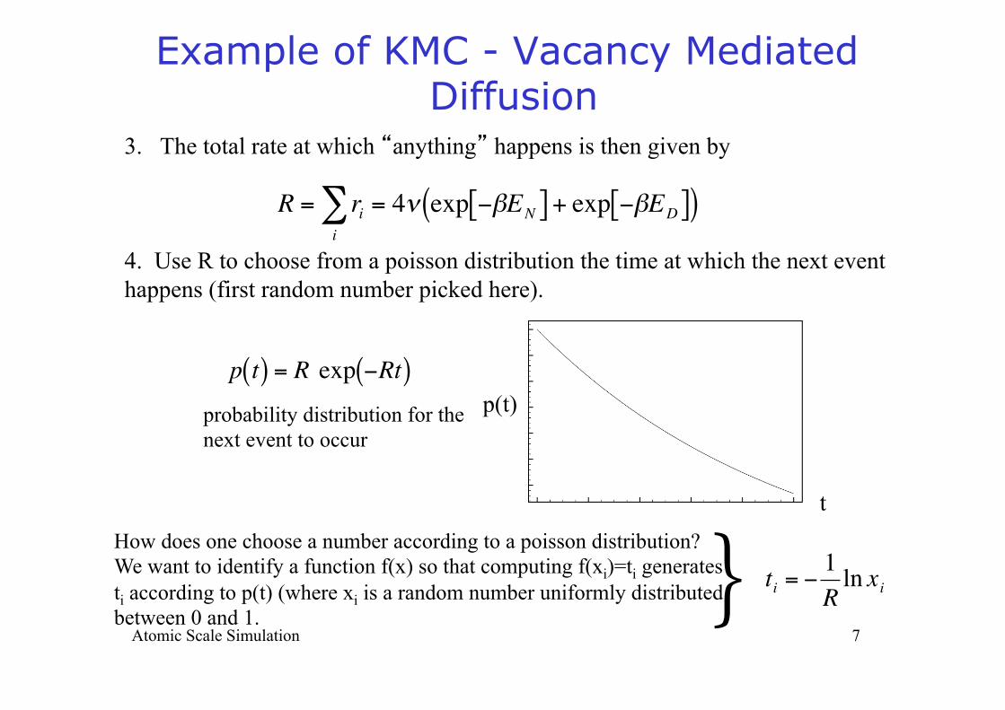
3. The total rate at which “anything” happens is then given by


€

R = rii∑ = 4ν exp −βEN[ ] + exp −βED[ ]( )

4. Use R to choose from a poisson distribution the time at which the next event happens (first random number picked here).

€

p t( ) = R exp −Rt( )probability distribution for the next event to occur

p(t)

t How does one choose a number according to a poisson distribution? We want to identify a function f(x) so that computing f(xi)=ti generates ti according to p(t) (where xi is a random number uniformly distributed between 0 and 1.

€

ti = −1Rln xi

€

}Atomic Scale Simulation 7


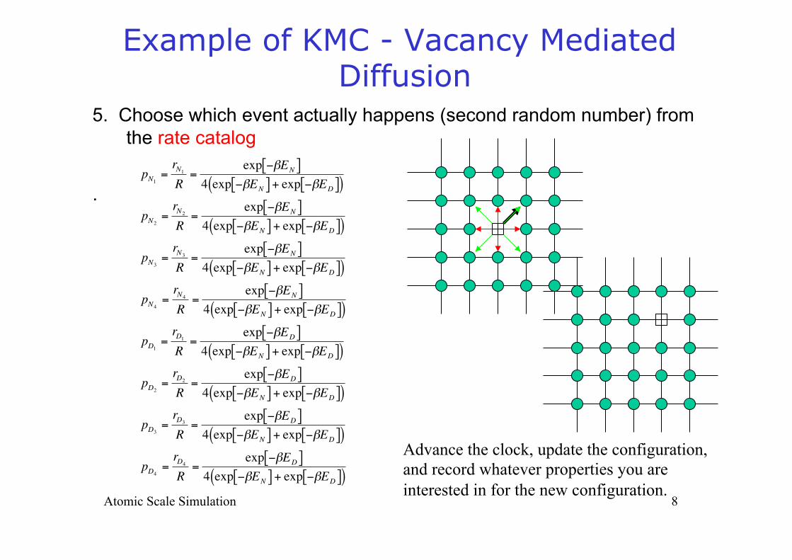
5. Choose which event actually happens (second random number) from the rate catalog

.

€

pN1 =rN1R

=exp −βEN[ ]

4 exp −βEN[ ] + exp −βED[ ]( )

pN2 =rN2R

=exp −βEN[ ]


pN3 =rN3R

=exp −βEN[ ]


pN4 =rN4R

=exp −βEN[ ]


pD1 =rD1R

=exp −βED[ ]


pD2 =rD2R

=exp −βED[ ]


pD3 =rD3R

=exp −βED[ ]


pD4 =rD4R

=exp −βED[ ]


Advance the clock, update the configuration, and record whatever properties you are interested in for the new configuration.



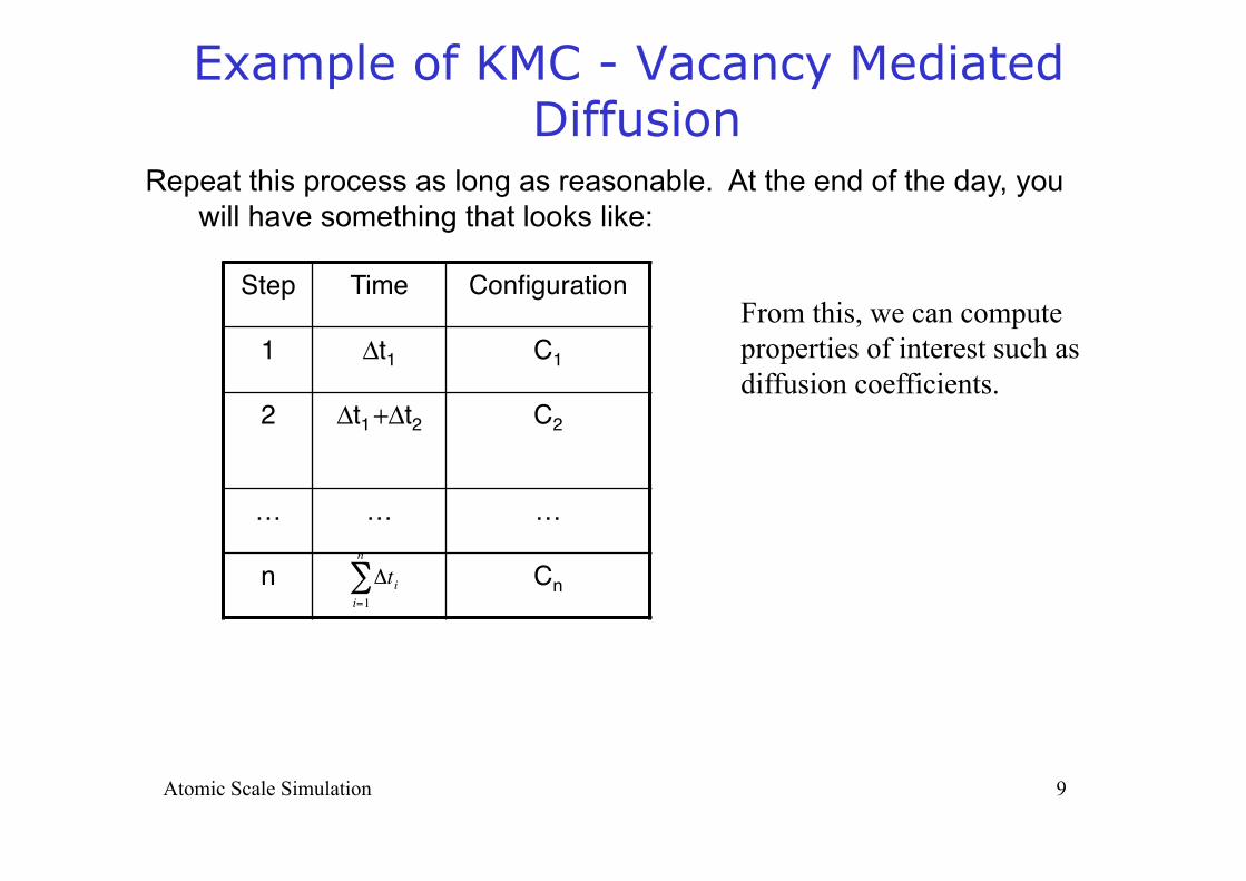
Repeat this process as long as reasonable. At the end of the day, you will have something that looks like:

Step Time Configuration

1 Δt1 C1

2 Δt1 +Δt2 C2

… … …

n Cn

€

Δtii=1

n

∑

From this, we can compute properties of interest such as diffusion coefficients.


Kinetic Monte Carlo vs. MD

MD: choose a potential, choose boundary conditions, and propagate the classical equations of motion forward in time. If potential is accurate, if electron-phonon coupling (non Born-Oppenheimer behavior) is negligible, then the dynamical evolution will be a very accurate representation of the real physical system.

Limitation is the time steps required by accurate integration (10-15 s to resolve atomic vibrations), generally limiting the total simulation time to microseconds.

KMC: attempts to overcome this by exploiting that the long-time dynamics of a system typically consist of jumps from one configuration to another.

In KMC, we do not follow trajectories, but treat the state transitions directly. Time scales are seconds or longer (in fact, achievable time varies with simulation temperature by orders of magnitude).

A key feature of KMC is that the configuration “sits” in some local minimum of configuration space for some time. It then transitions out of that state and into others with the transition rates related to the barriers. It does not matter how the system got into the current state in the first place - it is memoryless, and the process is Markovian.


What about the computational time in KMC?

Limited by searching through the rate catalog for the process that has been selected, so for the most elementary searches, KMC computational time will scale linearly with the number of processes. More sophisticated search algorithms can give log(M) scaling.

Why is KMC not exact?

- Inexact barriers. That is, inexactly computed.

- In fact, the TST rate is not exact (harmonic approximation to the minima & saddle point) but are pretty good (within 10-20%).

- Incomplete rate catalog. This is arguably the biggest problem in KMC. Our intuition cannot often capture surprising reaction pathways, and we neglect relevant physics.

Kinetic Monte Carlo vs. MD


Example: Adatom surface diffusion on Al(100)

•  Until 1990, diffusion of an adatom on an fcc(100) surface was thought to occur by a simple hopping from one site to another

•  Feibelman (1990) discovered using density functional calculations that the primary diffusion pathway is quite different

•  This new mechanism has now been observed for Pt(100) and Ir(100)

surfaces via field ion microscopy

After Voter, A.F. Radiation Effects in Solids, 2005:


13

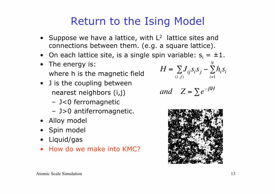
Return to the Ising Model •  Suppose we have a lattice, with L2 lattice sites and

connections between them. (e.g. a square lattice). •  On each lattice site, is a single spin variable: si = ±1. •  The energy is:

where h is the magnetic field •  J is the coupling between

nearest neighbors (i,j) –  J<0 ferromagnetic –  J>0 antiferromagnetic.

•  Alloy model •  Spin model •  Liquid/gas •  How do we make into KMC?

€

H = Jijsi(i , j )∑ sj − hisi

i=1

N∑

and Z = e–βH∑


14

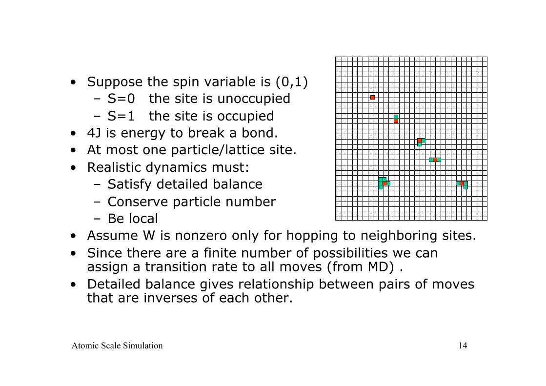
•  Suppose the spin variable is (0,1) –  S=0 the site is unoccupied –  S=1 the site is occupied

•  4J is energy to break a bond. •  At most one particle/lattice site. •  Realistic dynamics must:

–  Satisfy detailed balance –  Conserve particle number –  Be local

•  Assume W is nonzero only for hopping to neighboring sites. •  Since there are a finite number of possibilities we can

assign a transition rate to all moves (from MD) . •  Detailed balance gives relationship between pairs of moves

that are inverses of each other.


15

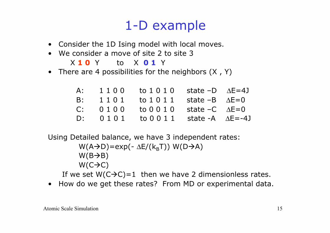
1-D example •  Consider the 1D Ising model with local moves. •  We consider a move of site 2 to site 3 X 1 0 Y to X 0 1 Y •  There are 4 possibilities for the neighbors (X , Y)

A: 1 1 0 0 to 1 0 1 0 state –D ΔE=4J B: 1 1 0 1 to 1 0 1 1 state –B ΔE=0 C: 0 1 0 0 to 0 0 1 0 state –C ΔE=0 D: 0 1 0 1 to 0 0 1 1 state -A ΔE=-4J

Using Detailed balance, we have 3 independent rates:

W(AàD)=exp(- ΔE/(kBT)) W(DàA) W(BàB) W(CàC)

If we set W(CàC)=1 then we have 2 dimensionless rates. •  How do we get these rates? From MD or experimental data.


16

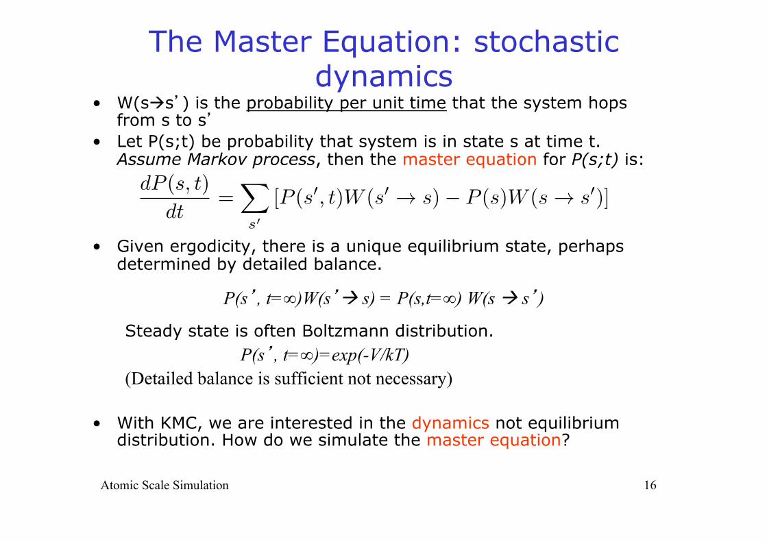
The Master Equation: stochastic dynamics

•  W(sàs’) is the probability per unit time that the system hops from s to s’

•  Let P(s;t) be probability that system is in state s at time t. Assume Markov process, then the master equation for P(s;t) is:

•  Given ergodicity, there is a unique equilibrium state, perhaps determined by detailed balance.

P(s’, t=∞)W(s’! s) = P(s,t=∞) W(s ! s’)

Steady state is often Boltzmann distribution. P(s’, t=∞)=exp(-V/kT) (Detailed balance is sufficient not necessary)

•  With KMC, we are interested in the dynamics not equilibrium distribution. How do we simulate the master equation?


dP (s, t)

dt=

X

s0

[P (s0, t)W (s0 ! s)� P (s)W (s ! s0)]

17

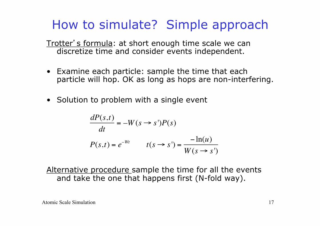
How to simulate? Simple approach Trotter’s formula: at short enough time scale we can

discretize time and consider events independent.

•  Examine each particle: sample the time that each particle will hop. OK as long as hops are non-interfering.

•  Solution to problem with a single event

Alternative procedure sample the time for all the events and take the one that happens first (N-fold way).

dP(s,t)dt

= –W (s→ s ')P(s)

P(s,t) = e–Wt t(s→ s ') = − ln(u)W (s→ s ')


18

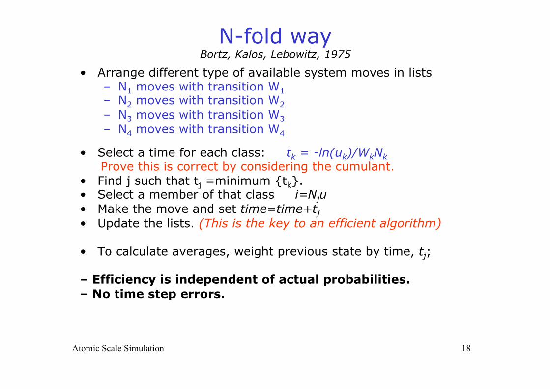
N-fold way Bortz, Kalos, Lebowitz, 1975

•  Arrange different type of available system moves in lists –  N1 moves with transition W1 –  N2 moves with transition W2 –  N3 moves with transition W3 –  N4 moves with transition W4

•  Select a time for each class: tk = -ln(uk)/WkNk Prove this is correct by considering the cumulant. •  Find j such that tj =minimum {tk}. •  Select a member of that class i=Nju •  Make the move and set time=time+tj •  Update the lists. (This is the key to an efficient algorithm)

•  To calculate averages, weight previous state by time, tj; – Efficiency is independent of actual probabilities. – No time step errors.


Documents

Kinetic Monte Carlo (KMC)