F U L L P A P E R

Kinetic energy density for orbital-free density functionalcalculations by axiomatic approach

Fahhad H. Alharbi1,2 | Sabre Kais1,2,3

1Qatar Environment and Energy Research

Institute (QEERI), Hamad Bin Khalifa

University, Doha, Qatar

2College of Science & Engineering (CSE),

Hamad Bin Khalifa University, Doha, Qatar

3Department of Chemistry, Physics, and

Birck Nanotechnology Center, Purdue

University, West Lafayette, Indiana

Correspondence

Fahhad H. Alharbi, College of Science &

Engineering (CSE), Hamad Bin Khalifa

University, Doha, Qatar.

Email: falharbi@hbku.edu.qa

AbstractAn axiomatic approach is herein used to determine the physically acceptable forms for general D-

dimensional kinetic energy density functionals (KEDF). The resulted expansion captures most of

the known forms of one-point KEDFs. By statistically training the KEDF forms on a model problem

of noninteracting kinetic energy in 1D (six terms only), the mean relative accuracy for 1000 ran-

domly generated potentials is found to be better than the standard KEDF by several orders of

magnitudes. The accuracy improves with the number of occupied states and was found to be bet-

ter than 1024 for a system with four occupied states. Furthermore, we show that free fitting of

the coefficients associated with known KEDFs approaches the exactly analytic values. The pre-

sented approach can open a new route to search for physically acceptable kinetic energy density

functionals and provide an essential step toward more accurate large-scale orbital free density

functional theory calculations.

K E YWORD S

kinetic energy density, kinetic energy density functionals, large-scale calculations, orbital-free den-

sity functional theory

1 | INTRODUCTION

Presently, density functional theory (DFT) dominates the field of atom-

istic and molecular quantum chemistry calculations.[1–3] This is mainly

due to its relatively low computational cost compared to many other

atomistic approaches. The mainstream DFT (i.e., Kohn–Sham DFT (KS-

DFT)[4]) is a slight alteration of the original work of Hohenberg and

Kohn (HK-DFT)[5] where it was proved that the ground state of any

many-electron system is completely characterized by its density and

the energy functional which permits the system to attain its minimum

at the density corresponding to the ground state. However, represent-

ing the contribution of the kinetic energy as a density functional

(KEDF) (T q xð Þ½ �5Ð t xð Þdx) where t xð Þ is the kinetic energy density

(KED) has proven to be challenging as the accuracy and applicability of

the presently proposed KEDF are generally not sufficient for reliable

calculations.[3,6–10] So, Kohn and Sham (KS-DFT) suggested an approxi-

mate approach where the “orbitals” are reintroduced such that the sum

of the orbitals densities equals to the exact density of the real system

and the kinetic energy is defined as the kinetic energy of the intro-

duced “fictitious” system. Computation-wise, this results in a conver-

sion of the problem from 3-dimensional (3D) to 3N-dimensional where

N orbitals are determined by solving the governing N23D equations

self-consistently and N is the number of electrons in the calculations.

Recently, the search for an orbital-free version of DFT (OF-DFT)

has rapidly gained attention.[11–15] To apply “orbital free” approaches, it

is essential to find highly accurate kinetic energy density functionals

(KEDF). The subject is not new and its origins date back to the early

years of quantum mechanics. Most of the early proposed KEDF are

based on particular exactly solvable models, for example, constant

potential with planewaves solution for Thomas–Fermi model (TF)[16,17]

or modified planewaves for von Weizsacker KEDF (vW).[18] This period

was followed by many extensions and further developments on “spe-

cific physical models.” For a comprehensive collection of suggested

functionals, we refer the reader to a review by Tran and Wesolow-

ski.[19] Alternatively, some of the recent developments adopted statisti-

cal techniques. For example, Burke and coworkers recently used

machine learning to approximate density functional[20,21] based on sta-

tistical expressions.

In this article, we revisit this from a different perspective. Instead

of starting from a specific physical model or using mathematical tools

to improve a KEDF, we begin by asking which forms of KEDF are

physically acceptable. To answer this query, an axiomatic approach is

Int J Quantum Chem. 2017;117:e25373.https://doi.org/10.1002/qua.25373

http://q-chem.org VC 2017Wiley Periodicals, Inc. | 1 of 9

Received: 21 December 2016 | Revised: 10 February 2017 | Accepted: 15 February 2017

DOI: 10.1002/qua.25373

used to determine the physically acceptable forms in a general D-

dimension space. In axiomatic approaches, a set of axioms are used in

conjunction to derive equations, expressions, or theorems.

As expected, the resulted expansion captures most of the known

forms of one-point KEDFs. By statistically training the forms for a

model problem of the noninteracting kinetic energy in 1D (six terms

only), we find that the mean relative accuracy for 1000 randomly gen-

erated potentials is orders of magnitudes better than that delivered by

standard KEDFs. The accuracy improves with the number of occupied

states, and it is better than 1024 at four occupied states. Furthermore,

it is shown that the free fitting of the coefficients associated with

known KEDFs approaches the exactly known values.

2 | KINETIC ENERGY DENSITY EXPANSIONFOR D-DIMENSIONAL SPACE

Herein, an axiomatic approach is used to derive an expansion of physi-

cally acceptable forms of KEDF that satisfy the following essential

physical requirements; dimensionality, finiteness, compatibility with the

virial theorem, and non-negativity of t xð Þ. Also, the functional deriva-

tive of the final expansion will be derived as it is needed for efficient

energy minimization.

2.1 | The expression of t xð Þ as a function of density

derivatives

Generally, t xð Þ can be defined as a scalar function of the density and

its derivatives, that is,

t xð Þ � f q;rq;r2q; � � � ;rðnÞq� �

: (1)

For the 1-dimensional case (1D), Shao and Baltin[22] proved that the

highest derivative order is 1 and all the derivatives for n>1 must be

ruled out based on the compatibility with the differential virial

theorem[23–25] and t xð Þ non-negativity. The same concept can be fur-

ther extended to D-dimensional cases.

Here, we outline Shao and Baltin[22] proof for 1D case and how it

is extended to D-dimension. In 1D, the differential virial theorem of fer-

mionic system with Coulombic interaction is

qðxÞv0ðxÞ514q00022 t0ðxÞ : (2)

At the beginning, we need to represent the above equation in terms of

the density and its derivatives only. t0ðxÞ, which is directly obtained

from Equation 1 (for 1D), is

t0ðxÞ5Xnm50

qðm11Þ ofoqðmÞ

(3)

As for v0ðxÞ, it is obtained by taking the derivative of Euler equation

when applying Equation 1 within DFT framework. So,

ddx

dE½q�dq

� �50 (4)

and hence

v0ðxÞ52ddx

dE½q�dq

� �5Xnm50

ð21Þm11 dm11

dxm11

ofoqðmÞ

� �(5)

Here, we used the fact that the chemical potential l is constant and

hence its derivative is zero. By inserting Equations 3 and 5 in Equation

2, it becomes

Xnm50

ð21Þm11qdm11

dxm11

ofoqðmÞ

� �12qðm11Þ of

oqðmÞ

� �514q000 (6)

Finally, the left-hand side of the above equation are rearranged[22] and

due to the fact that only q000 appears on the right-hand side, it is found

that for any n � 2,

o2f

o qðnÞ½ �250 : (7)

This implies that f must be linear with respect of qðnÞ. This clearly viola-

tes the non-negativity of KED and hence the dependence of f on qðnÞ

must be ruled out.

The extension of the above proof to higher dimensions is concep-

tually straightforward; but more tedious mathematically. First, the dif-

ferential virial theorem is extended to D-dimension,[25] and it becomes:

qðxÞ dvdxa

514

ddxa

r2q�

2za (8)

where

za5XDb51

oox0b

1oox00b

!o2g x1x0; x1x00ð Þ

ox0aox00b

jx05x0050 (9)

and g x1x0; x1x00ð Þ is the one-particle density matrix. za can be decom-

posed into two parts as follow:

za52dtdxa

1~za (10)

Then, we take the derivative of Euler equation in D-dimesion. The

resulted equation is

dvdxa

5Xnm50

ð21Þm11 ddxa

rm ofo rmq½ �� �� �

(11)

Finally, by inserting the above equations in the differential virial equa-

tion (Equation 8). It can be rewritten as

Xnm50

ð21Þm11qddxa

rm ofo rmq½ �� �� �

12d rmq½ �dxa

ofo rmq½ �

� �1~za5

14

ddxa

r2q� (12)

With further arrangement and because only ddxa

r2q�

term appears on

the right-hand side, it can be shown that

o2f

o rnq½ �250 : (13)

for n � 2. Again, this implies that f must be linear with respect of rnq

and this clearly violates the non-negativity of KED. Thus, it must be

ruled out.

Conversely, the Laplacian (beside the gradient) arises naturally

from the definition of kinetic energy operator.[8] However, there

exists some ambiguity concerning it.[8,12,26] As for t xð Þ, unphysical

2 of 9 | ALHARBI AND KAIS

pathological negativity arises if the dependence on r2q is of

odd-power and r2q is negative itself. This agrees with the conclu-

sion of Shao and Baltin eliminating dependence on r2q. Thus, the

scalar function compatible with the differential virial theorem

becomes

t xð Þ � f q;rqð Þ : (14)

In addition, it is known that the spatial extension of the density

plays an important role in t xð Þ. Previously, this was accounted for

by using either the total number of electrons N or the physical

coordinates, x (please see Ref. 16 and the references within). Using

N—as a number— ignores details associated with q xð Þ while the

explicit inclusion of x violates the invariance under co-ordinate

transformations. In this work, we incorporate the effect of the spa-

tial extension of the density by a single measure, rd, which is related

to the trace of the covariance matrix r5½rij�. It is defined conven-

tionally as:

r2d51D

XDi

r2ii ; (15)

where:

r2ij5

ÐqðxÞ xi2lið Þ xj2lj

� dxÐ

qðxÞdx (16)

and

li5

ÐqðxÞ xi dxÐqðxÞdx : (17)

By inserting Equations 16 and 17 in Equation 15, it becomes

r2d51D

Ð ÐqðxÞqðx0Þ x � x2x0ð Þdxdx0Ð

qðxÞdx �2 : (18)

Equation 18 may simply be reduced to the normalized standard devia-

tion in the 1-dimensional case. Thus, the spatial extension is derived

solely from qðxÞ. More interestingly, the consideration of the spatial

extension leads to an additional origin of nonlocality in KEDF as antici-

pated by many.[3,27–32] This shall be investigated further in a future

work.

However, it is important to highlight that rd could result in some

inconsistencies. The covariance matrix, r, (which is used to estimate

rd) accounts for many spatial aspects concurrently. As an example, it

accounts for the spatial dispersion of a single clustered density. On

the contrary, in the case of a pair of “nonoverlapping densities,” r is

dominated by the distance between the centers of the two densities

rather than their individual spatial extensions. Thus, there is still a

need to have a more consistent “measure” for the spatial extension

of the density. This shall not alter the form of KEDF; however, dTdq

must be modified according to the new conventionally defined

“measure.”

With all these considerations plus the scalar nature of t xð Þ, a possi-ble general expansion of KEDF is given by:

t xð Þ5Xsln

asln1rsdq

lD rq � rqð Þn=2; (19)

where asln are the expansion coefficients and shall be determined

through statistical training.

2.2 | The limits of the sum

Obviously, the general expansion (Equation 19) may have infinite terms

as s, l, and n can take any integer value. However, this is governed by

physics and hence there are limits and interconnections between the

three indices. By seeking the proper dimensionality of t xð Þ (L2D22 in

atomic unit, where L is the dimension of the length), it is found that:

l5 22s2nð Þ1 12nð ÞD ; (20)

This permits a description of l entirely in terms of s and n hence the

expansion is reduced to:

t xð Þ5Xsn

asn1rsdq

1D 22s2nð Þ1 12nð ÞD½ � rq � rqð Þn=2 : (21)

The limits of the sum are determined by other essential physical

considerations. Fundamentally, since qðxÞ is finite, n must be non-

negative. Concerning s, for uniform density—which is a proper quantum

mechanical case— rd ! 1; thus, s must be non-negative as well. The

upper limits of s and n are determined by considering finite systems

where q xð Þ vanishes exponentially. For such systems, qðxÞ5fðxÞexp2j

ffiffiffiffiffix2

p� �where j is positive and nonzero. By applying this restriction,

it can be shown that for such systems, Equation 19 is further reduced

to:

t xð Þ5Xsn

asnrsd

flD1 rf � rf1j2f222j f

rf � xx2

� �n=2" #

3exp

(2

lD1n

� �jffiffiffiffiffix2

p ):

(22)

By forcing t xð Þ to vanish at infinity,

lD1n>0 ; (23)

and by using Equation 20, we are lead to

s1n<D12 ; (24)

by using Equation 20. This defines the upper limits of each expansion

iterator. So, the general form Equation 19 is reduced to the following

expansion in D-dimensional space:

t xð Þ5XD11

s50

XD112s

n50

asn1rsdq

1D 22s2nð Þ1 12nð ÞD½ � rq � rqð Þn=2 : (25)

This expansion captures most of the known forms of one-point KEDFs.

For example, by setting, s5n50, the resulted form qðD12Þ=D, which is

simply TF KEDF in D-dimension. If s50 and n52, the resulted KEDF

is vW, that is, jrqj2=q.The axiomatic approach determines the possible KEDF forms that

satisfy the essential physical requirements of dimensionality and finite-

ness. But, the expansion coefficients, ans, must be determined by other

means. In this work, we will determine these ans statistically in an

ALHARBI AND KAIS | 3 of 9

analogous method to the machine learning approach. However, the

derived functional forms are in principal universal and their coefficients

must be accordingly universal. Later, we will show that this statistical

approach leads to the properly known coefficients in the cases of the

TF and vW limits.

2.3 | The functional derivative

As the application of DFT requires the minimization of the total energy

as a functional of the density and subjected to some constraints, we

must find the functional derivative of the kinetic energy functional:

T½q xð Þ�5Ð t xð Þdx : (26)

Using the general derived form of t xð Þ as in Equation 25, we found

that:

dTdq

5XD11

s50

XD112s

n50

asn1rsd

(q

lD rq � rqð Þn=222

lD

12nð Þ1q

rq � rqð Þ22n rq � rqð Þr2q2n2

n22ð Þ rq � r rq � rqð Þ½ �� �

1sÐqðx0Þ l

D rqðx0Þ � rqðx0Þð Þn=2dx0

1Ðqðx0Þdx0 2

12

Ðqðx0Þ x2x0ð Þ � x2x0ð Þdx0Ð Ð

qðx0Þqðx00 Þ x0 � x02x00ð Þdx0 dx00

� �):

(27)

3 | RESULTS AND DISCUSSION FOR 1DCASES

In this work, we consider only noninteracting fermions in one-

dimension where the occupied states are assumed to be doubly and

fully occupied closed-shell. In such case, Equations 25 and 27 are

reduced to:

t xð Þ5X2s50

X22s

n50

asn1rsdq 32s22nð Þ q

02� �n=2

(28)

and

dTdq

5X2s50

X22s

n50

asn1rsd

(32s22nð Þ 12nð Þq 22s22nð Þ q

02� �n=2

2n n21ð Þq 32s22nð Þ q02

� � n221

� �q00

1sÐq 32s22nð Þ q

02� �n=2

dx0

1Ðqðx0Þdx0 2

12

Ðqðx0Þ x2x0ð Þ2dx0Ð Ð

qðx0Þqðx00 Þ x0 x02x00ð Þ dx0 dx00

" #)(29)

FIGURE 1 The statistical method used to determine theexpansion coefficients that are then applied in t xð Þ to calculate thekinetic energy and to implement DFT minimization

TABLE 1 The expansion terms of KED in 1D

s n KED

0 0 q3

0 1 qjq0j0 2 q0ð Þ2

q

1 0 1rdq2

1 1 1rdjq0j

2 0 1r2d

q

FIGURE 2 The relative error in the noninteracting kinetic energyTs. The top three piles are for full fitting where three upper limitsof s are assumed; namely 0, 1, and 2. The middle set of three pilesare for the case where we use a005p2=24 and a0251=8 to enforcethe TF and vW (TFvW) limits, respectively. The last three piles arefor the standard TF, vW, and TFvW models

4 of 9 | ALHARBI AND KAIS

The resulted expansion terms of 1D KEDF are shown in Table 1.

However, we still need a mechanism to determine the expansion coef-

ficients. In principle, these coefficients must be universal and should be

determined entirely by physical consideration. For example, in the TF

limit, the known coefficient for q3 (TF model) is a005p2=24 while a025

1=8 is the vW coefficient. However, and aforementioned in this work,

these coefficients are determined statistically by using training sets of

known kinetic energies and densities for given potentials. Then, these

coefficients are used to calculate the kinetic energy for a new set of

“test” potentials using t xð Þ with densities both numerically obtained by

solving Schr€odinger equation and resulting from DFT minimization.

This process is represented schematically in Figure 1. It was found that

the expansion coefficients converged rapidly with the size of the train-

ing set for a given number of occupied states. To guarantee consis-

tency, training sets of 1000 potentials are used throughout this article.

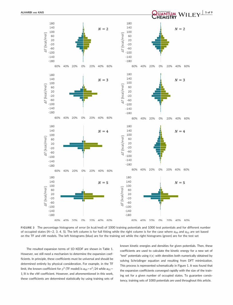
FIGURE 3 The percentage histograms of error (in kcal/mol) of 1000 training potentials and 1000 test potentials and for different numberof occupied states (N52; 3; 4; 5). The left column is for full fitting while the right column is for the case where a00 and a02 are set basedon the TF and vW models. The left histograms (blue) are for the training set while the right histograms (green) are for the test set

ALHARBI AND KAIS | 5 of 9

The considered class of potentials is the one used by Burke and

coworkers which consists of three different Gaussian dips (GD) con-

fined to a 1D box of length L51 and between two infinite walls.[20,33]

This class of potentials possesses the functional form:

vðxÞ52X3i51

ai exp2 x2bið Þ2

2c2i

" #; (30)

where ai, bi, and ci are generated randomly, and obey the following

constraints: 1<a<10; 0:4<b<0:6, and 0:03<c<0:1. An efficient spec-

tral method is used to solve for the states and hence the densities with

an accuracy greater than 10212 for the exact noninteracting kinetic

energy (Ts).[34,35]

3.1 | T½q� Calculated using the density numerically

obtained through solving the Schr€odinger equation

A thousand potentials are generated and solved; the exact Ts is then

calculated for various numbers of occupied states (N52; 3; 4; 5). The

Exact Ts are used to find the best least square fitting for the expansion

coefficients. Figure 2 gives the performance of the expansion in terms

of mean relative error (jTs2Ð L0 tðqðxÞÞdxj=Ts). The top three piles are for

full fitting where three upper limits of s are assumed; namely 0, 1, and

2. The middle set of three piles are for the case where we use a005p2=

24 and a0251=8 to enforce the TF and vW (TFvW) limits, respectively.

The last three piles are for the standard TF, vW, and TFvW models.

Clearly, the new expansion (Equation 25) results in better perform-

ance when compared to the standard models by at least two orders of

magnitude. The accuracy is improved further as the number of the

occupied states increases. Also, it is clear that the consideration of the

spatial extension of the density—using rd—improves the estimation

even further. Note that only four parameters (six under the case of full

fitting) are needed to very accurately estimate the noninteracting

kinetic energy for 1000 potentials with four different occupied states.

The second analysis was designed to test the validity of the expan-

sion. At the beginning, 1000 training potentials are used to find the

expansion coefficients. These are then used to estimate T directly for

another 1000 test potentials for N52; 3; 4; 5. The results are shown

in Figure 3 where the left histograms (blue) are for the training set

while the right histograms (green) are for the test set. The left column

is for full fitting while the right column is for the case where a00 and

a02 are set to p2=24 and 1/8 and only four parameters are statically

determined. Here, the error is given in kcal/mol. Distinctly, the statisti-

cally trained expansion coefficients were able to estimate Ts very accu-

rately. The errors mean absolute, standard deviation, and max absolute

are shown in Table 2 and are given in kcal/mol. However, they are still

much beyond the chemical accuracy limit (1 kcal/mol). Furthermore

and as aforementioned, the family of potentials used is the same as

was used by Burke and coworkers to find KEDF with machine learn-

ing.[20,33] In that work, they used a process containing around 100 000

empirical parameters. They achieved accuracies below 1 kcal/mol and

two order of magnitudes better than what is obtained in this work.

However to iterate, in this work we used only six parameters.

3.2 | T½q� Calculated using the density resulted from

DFT minimization

In the previous subsection, the exact density (as calculated using high

order spectral methods) are used to estimate the kinetic energy.

TABLE 2 The errors mean absolute (jDTj), standard deviation(jDTjstd), and max absolute (jDTjmax) in kcal/mol

NFullfitting

Fittingwith TFvW

jDTj jDTjstd jDTjmax jDTj jDTjstd jDTjmax

2 40.4 38.0 283.4 38.9 37.4 344.3

3 22.3 21.7 164.0 37.9 35.8 330.1

4 11.9 10.4 89.0 53.6 47.2 268.1

5 12.0 10.1 55.4 19.1 18.9 123.2

FIGURE 4 The calculated densities from energy minimization using both full fitting (blue lines) and the fitting with forced TFvW (red lines)beside the exact density (black lines) for two randomly generated potentials and for various number of occupied states (N52, 3, 4, as 5 asindicated in the top right side of each of the panels). The top set is for the first potential (shown in the top left panel) while the bottom setis for the second potential (shown in the bottom left panel)

6 of 9 | ALHARBI AND KAIS

However in DFT, it is essential to find the density that minimize the

energy while maintaining the number of involved particles. There are

many possible techniques.[36,37] In this work, we use a gradient-based

trust-region self-consistent method.[38–41] Figure 4 shows the calcu-

lated densities resulted from energy minimization using both full fitting

and the fitting with forced TFvW beside the exact density for two ran-

domly generated potentials and for various number of occupied states

(N52, 3, 4, as 5). It is clear that the suggested t xð Þ (as tested in 1D

cases) accurately produces the minimum densities. Also, the results of

full fitting are better that those of the fitting with imposed TFvW

parameters. However, the main outcome is its capacity to maintain the

shell structure, which is challenging for the standard approximation

based on TFvW models.

Energy minimization is then applied to find the densities and the

kinetic energies of the 1000 systems used in the previous subsection

for N52; 3; 4; 5. The results are shown in Figure 5 where the left

FIGURE 5 The percentage histograms of error in relative values (left column) and in kcal/mol (right column) of 1000 potentials and fordifferent number of occupied states (N52; 3; 4; 5). In each panel, the left side (blue) is for the full fitting while the right one (green) is forthe fitting with TFvW imposed

ALHARBI AND KAIS | 7 of 9

column shows the relative error while the right column shows the

absolute error in kcal/mol. In each panel, the left side (blue) is for the

full fitting while the right one (green) is for the fitting with TFvW

imposed. As can be seen, the error is less than 1% and in most cases, it

is less than 0.1%. However, this is large as absolute value. Also as

observed in the previous subsection, it is clear that full fitting results in

more accurate calculations as expected from the calculated densities

by DFT minimization. There could be many causes for the increased

accuracy beside the additional degrees of freedom allowed by full fit-

ting. However, we believe that this could be a numerical error due to

the shape optimization. This becomes more apparent for higher occu-

pied states.

3.3 | On the expansion coefficients

As stated earlier, the expansion coefficients are determined statistically

in this work. However, they must be universal. The only two known

parameters are a00 which equal to p2=24 (TF KEDF) and a02 which

equal to 1/8 (vW KEDF). vW KEDF must be equal to Ts for single occu-

pied states. Thus, a fitting for various potentials with single occupied

state must get reduced to vW KEDF. This was obtained for various

number of training potentials while the other expansion coefficients in

this case are fitted trivially to zero. However, they must not all vanish.

Rather, the collective contributions of all the other KEDF terms—in this

limit—must vanish.

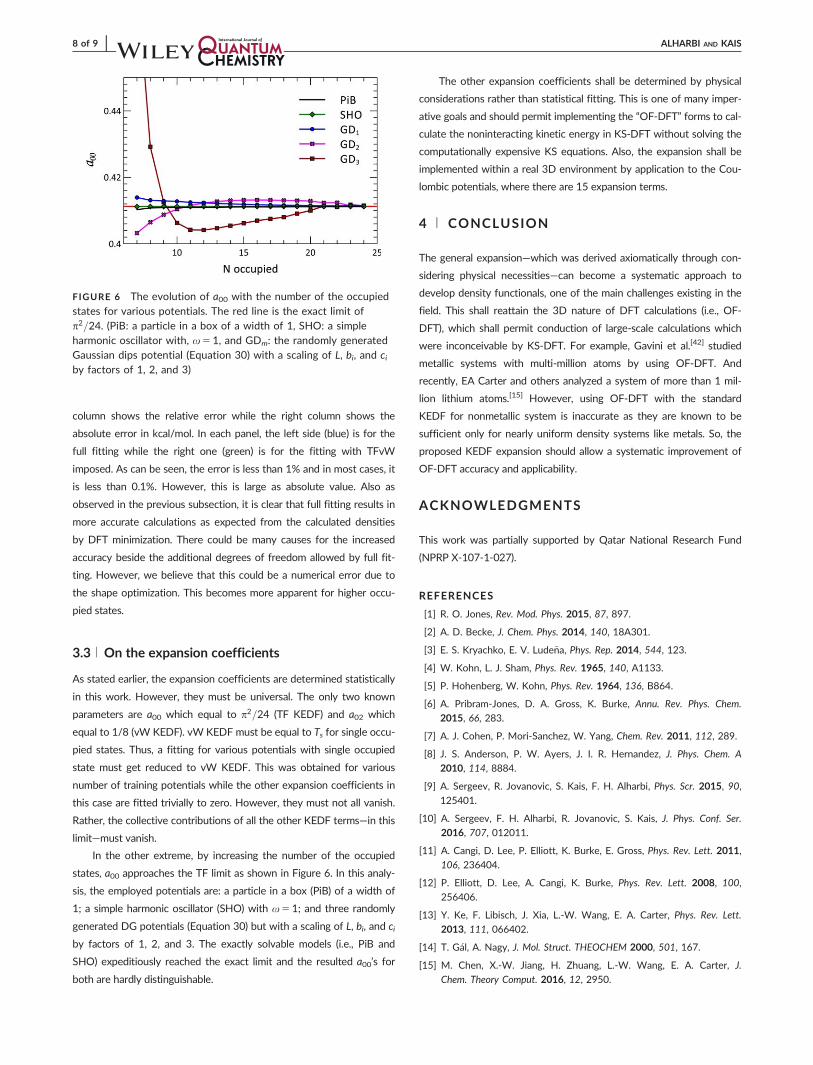
In the other extreme, by increasing the number of the occupied

states, a00 approaches the TF limit as shown in Figure 6. In this analy-

sis, the employed potentials are: a particle in a box (PiB) of a width of

1; a simple harmonic oscillator (SHO) with x51; and three randomly

generated DG potentials (Equation 30) but with a scaling of L, bi, and ci

by factors of 1, 2, and 3. The exactly solvable models (i.e., PiB and

SHO) expeditiously reached the exact limit and the resulted a00’s for

both are hardly distinguishable.

The other expansion coefficients shall be determined by physical

considerations rather than statistical fitting. This is one of many imper-

ative goals and should permit implementing the “OF-DFT” forms to cal-

culate the noninteracting kinetic energy in KS-DFT without solving the

computationally expensive KS equations. Also, the expansion shall be

implemented within a real 3D environment by application to the Cou-

lombic potentials, where there are 15 expansion terms.

4 | CONCLUSION

The general expansion—which was derived axiomatically through con-

sidering physical necessities—can become a systematic approach to

develop density functionals, one of the main challenges existing in the

field. This shall reattain the 3D nature of DFT calculations (i.e., OF-

DFT), which shall permit conduction of large-scale calculations which

were inconceivable by KS-DFT. For example, Gavini et al.[42] studied

metallic systems with multi-million atoms by using OF-DFT. And

recently, EA Carter and others analyzed a system of more than 1 mil-

lion lithium atoms.[15] However, using OF-DFT with the standard

KEDF for nonmetallic system is inaccurate as they are known to be

sufficient only for nearly uniform density systems like metals. So, the

proposed KEDF expansion should allow a systematic improvement of

OF-DFT accuracy and applicability.

ACKNOWLEDGMENTS

This work was partially supported by Qatar National Research Fund

(NPRP X-107-1-027).

REFERENCES

[1] R. O. Jones, Rev. Mod. Phys. 2015, 87, 897.

[2] A. D. Becke, J. Chem. Phys. 2014, 140, 18A301.

[3] E. S. Kryachko, E. V. Lude~na, Phys. Rep. 2014, 544, 123.

[4] W. Kohn, L. J. Sham, Phys. Rev. 1965, 140, A1133.

[5] P. Hohenberg, W. Kohn, Phys. Rev. 1964, 136, B864.

[6] A. Pribram-Jones, D. A. Gross, K. Burke, Annu. Rev. Phys. Chem.

2015, 66, 283.

[7] A. J. Cohen, P. Mori-Sanchez, W. Yang, Chem. Rev. 2011, 112, 289.

[8] J. S. Anderson, P. W. Ayers, J. I. R. Hernandez, J. Phys. Chem. A

2010, 114, 8884.

[9] A. Sergeev, R. Jovanovic, S. Kais, F. H. Alharbi, Phys. Scr. 2015, 90,

125401.

[10] A. Sergeev, F. H. Alharbi, R. Jovanovic, S. Kais, J. Phys. Conf. Ser.

2016, 707, 012011.

[11] A. Cangi, D. Lee, P. Elliott, K. Burke, E. Gross, Phys. Rev. Lett. 2011,

106, 236404.

[12] P. Elliott, D. Lee, A. Cangi, K. Burke, Phys. Rev. Lett. 2008, 100,

256406.

[13] Y. Ke, F. Libisch, J. Xia, L.-W. Wang, E. A. Carter, Phys. Rev. Lett.

2013, 111, 066402.

[14] T. G�al, A. Nagy, J. Mol. Struct. THEOCHEM 2000, 501, 167.

[15] M. Chen, X.-W. Jiang, H. Zhuang, L.-W. Wang, E. A. Carter, J.

Chem. Theory Comput. 2016, 12, 2950.

FIGURE 6 The evolution of a00 with the number of the occupied

states for various potentials. The red line is the exact limit ofp2=24. (PiB: a particle in a box of a width of 1, SHO: a simpleharmonic oscillator with, x51, and GDm: the randomly generatedGaussian dips potential (Equation 30) with a scaling of L, bi, and ciby factors of 1, 2, and 3)

8 of 9 | ALHARBI AND KAIS

[16] L. H. Thomas, Math. Proc. Camb. Philos. Soc. 1927, 23, 542.

[17] E. Fermi, Z. Phys. 1928, 48, 73.

[18] C. von Weizsäcker, Z. Phys. A Hadrons Nucl. 1935, 96, 431.

[19] F. Tran, T. A. Wesolowski, Recent Progress in Orbital-Free Density

Functional Theory, World Scientific, Singapore 2013, p. 429.

[20] J. C. Snyder, M. Rupp, K. Hansen, K.-R. M€uller, K. Burke, Phys. Rev.

Lett. 2012, 108, 253002.

[21] J. C. Snyder, M. Rupp, K. Hansen, L. Blooston, K.-R. M€uller, K.

Burke, J. Chem. Phys. 2013, 139, 224104.

[22] J. Shao, R. Baltin, J. Phys. A Math. Gen. 1990, 23, 5939.

[23] I. G. Ryabinkin, V. N. Staroverov, Int. J. Quantum Chem. 2013, 113,

1626.

[24] A. Holas, N. March, Phys. Rev. A 1995, 51, 2040.

[25] A. Holas, N. March, Phys. Chem. Liquids 2006, 44, 465.

[26] E. Sim, J. Larkin, K. Burke, C. W. Bock, J. Chem. Phys. 2003, 118,8140.

[27] C. Huang, E. A. Carter, Phys. Rev. B 2010, 81, 045206.

[28] E. Chac�on, J. Alvarellos, P. Tarazona, Phys. Rev. B 1985, 32, 7868.

[29] L.-W. Wang, M. P. Teter, Phys. Rev. B 1992, 45, 13196.

[30] Y. A. Wang, N. Govind, E. A. Carter, Phys. Rev. B 1998, 58, 13465.

[31] F. Perrot, J. Phys. Condens. Matter 1994, 6, 431.

[32] M. Plumer, D. Geldart, J. Phys. C Solid State Phys. 1983, 16, 677.

[33] L. Li, J. C. Snyder, I. M. Pelaschier, J. Huang, U.-N. Niranjan, P. Dun-

can, M. Rupp, K.-R. M€uller, K. Burke, Int. J. Quantum Chem. 2016,

116, 819.

[34] F. Alharbi, Phys. Lett. A 2010, 374, 2501.

[35] F. H. Alharbi, S. Kais, Phys. Rev. E 2013, 87, 043308.

[36] H. B. Schlegel, Wiley Interdiscip. Rev. Comput. Mol. Sci. 2011, 1, 790.

[37] L. Fan, T. Ziegler, J. Chem. Phys. 1991, 95, 7401.

[38] L. Thøgersen, J. Olsen, D. Yeager, P. Jørgensen, P. Sałek, T. Hel-

gaker, J. Chem. Phys. 2004, 121, 16.

[39] J. B. Francisco, J. M. Martínez, L. Martínez, J. Chem. Phys. 2004,

121, 10863.

[40] Y. Saad, J. R. Chelikowsky, S. M. Shontz, SIAM Rev. 2010, 52, 3.

[41] R. H. Byrd, J. C. Gilbert, J. Nocedal, Math. Program. 2000, 89, 149.

[42] V. Gavini, K. Bhattacharya, M. Ortiz, J. Mech. Phys. Solids 2007, 55,

697.

How to cite this article: Alharbi FH, Kais S. Kinetic energy den-

sity for orbital-free density functional calculations by axiomatic

approach. Int J Quantum Chem. 2017;117:e25373. https://doi.

org/10.1002/qua.25373

ALHARBI AND KAIS | 9 of 9