arX

iv:a

stro

-ph/

0703

542v

1 2

0 M

ar 2

007

Kinetic Effects on Turbulence Driven by

the Magnetorotational Instability in Black

Hole Accretion

Prateek Sharma

A Dissertation

Presented to the Faculty

of Princeton University

in Candidacy for the Degree

of Doctor of Philosophy

Recommended for Acceptance

by the department of

Astrophysical sciences

September 2006

c© Copyright by Prateek Sharma, 2008.

All Rights Reserved

Abstract

Many astrophysical objects (e.g., spiral galaxies, the solar system, Saturn’s rings,

and luminous disks around compact objects) occur in the form of a disk. One of

the important astrophysical problems is to understand how rotationally supported

disks lose angular momentum, and accrete towards the bottom of the gravitational

potential, converting gravitational energy into thermal (and radiation) energy.

The magnetorotational instability (MRI), an instability causing turbulent trans-

port in ionized accretion disks, is studied in the kinetic regime. Kinetic effects are

important because radiatively inefficient accretion flows (RIAFs), like the one around

the supermassive black hole in the center of our Galaxy, are collisionless. The ion

Larmor radius is tiny compared to the scale of MHD turbulence so that the drift

kinetic equation (DKE), obtained by averaging the Vlasov equation over the fast gy-

romotion, is appropriate for evolving the distribution function. The kinetic MHD

formalism, based on the moments of the DKE, is used for linear and nonlinear stud-

ies. A Landau fluid closure for parallel heat flux, which models kinetic effects like

collisionless damping, is used to close the moment hierarchy.

We show that the kinetic MHD and drift kinetic formalisms give the same set

of linear modes for a Keplerian disk. The BGK collision operator is used to study

the transition of the MRI from kinetic to the MHD regime. The ZEUS MHD code

iii

is modified to include the key kinetic MHD terms: anisotropic pressure tensor and

anisotropic thermal conduction. The modified code is used to simulate the collisionless

MRI in a local shearing box. As magnetic field is amplified by the MRI, pressure

anisotropy (p⊥ > p‖) is created because of the adiabatic invariance (µ ∝ p⊥/B).

Larmor radius scale instabilities—mirror, ion-cyclotron, and firehose—are excited

even at small pressure anisotropies (∆p/p ∼ 1/β). Pressure isotropization due to

pitch angle scattering by these instabilities is included as a subgrid model. A key

result of the kinetic MHD simulations is that the anisotropic stress can be as large as

the Maxwell stress.

It is shown, with the help of simple tests, that the centered differencing of anisotropic

thermal conduction can cause the heat to flow from lower to higher temperatures,

giving negative temperatures in regions with large temperature gradients. A new

method, based on limiting the transverse temperature gradient, allows heat to flow

only from higher to lower temperatures. Several tests and convergence studies are

presented to compare the different methods.

iv

Acknowledgements

I foremost thank my adviser Greg Hammett, whose guidance made this thesis possible.

His insight, quest for perfection, and passion for science has always inspired me. He

was always patient, and ensured that I understood every subtle point. Thanks to

Eliot Quataert, who is an inspiring mentor, and initiated me into the fascinating field

of astrophysics. He was so accessible that I never felt that he was not in Princeton.

I am thankful to Jim Stone for his constant encouragement, and help with numerical

methods, especially ZEUS.

Finally, thanks to my loving and supporting family, and wonderful friends. Special

thanks to my brother Rohit, sister Chubi, and cousins, who have always brought joy

in my life. My wife Asha has been a loving and caring companion; her suggestion to

keep it simple has significantly improved the thesis.

The thesis work was supported by U.S. DOE contract # DE-AC02-76CH03073,

and NASA grants NAG5-12043 and NNH06AD01I. Many thanks to the NASA web-

sites for amazing pictures, some of which I have used in this thesis.

v

To my parents and grandparents

vi

Contents

Abstract . . . . . . . . . . . . . . . . . . . . . . . . . . . . . . . . . . . . . iii

Acknowledgements . . . . . . . . . . . . . . . . . . . . . . . . . . . . . . . v

1 Introduction 5

1.1 Accretion as an energy source . . . . . . . . . . . . . . . . . . . . . . 8

1.1.1 The Eddington limit . . . . . . . . . . . . . . . . . . . . . . . 9

1.1.2 The emitted spectrum . . . . . . . . . . . . . . . . . . . . . . 10

1.2 Accretion disk phenomenology . . . . . . . . . . . . . . . . . . . . . . 11

1.2.1 Governing equations . . . . . . . . . . . . . . . . . . . . . . . 13

1.2.2 Fluctuations . . . . . . . . . . . . . . . . . . . . . . . . . . . . 15

1.2.3 α disk models . . . . . . . . . . . . . . . . . . . . . . . . . . . 17

1.3 MRI: the source of disk turbulence . . . . . . . . . . . . . . . . . . . 18

1.3.1 Insufficiency of hydrodynamics . . . . . . . . . . . . . . . . . . 18

1.3.2 MHD accretion disks: Linear analysis . . . . . . . . . . . . . . 20

1.3.3 MHD accretion disks: Nonlinear simulations . . . . . . . . . . 25

1.4 Radiatively inefficient accretion flows . . . . . . . . . . . . . . . . . . 29

1.4.1 RIAF models . . . . . . . . . . . . . . . . . . . . . . . . . . . 33

1.4.2 The Galactic center . . . . . . . . . . . . . . . . . . . . . . . . 36

1.5 Motivation . . . . . . . . . . . . . . . . . . . . . . . . . . . . . . . . . 38

1.6 Overview . . . . . . . . . . . . . . . . . . . . . . . . . . . . . . . . . . 40

vii

2 Description of collisionless plasmas 44

2.1 The Vlasov equation . . . . . . . . . . . . . . . . . . . . . . . . . . . 45

2.2 The drift kinetic equation . . . . . . . . . . . . . . . . . . . . . . . . 46

2.3 Kinetic MHD equations . . . . . . . . . . . . . . . . . . . . . . . . . 48

2.4 Landau fluid closure . . . . . . . . . . . . . . . . . . . . . . . . . . . 49

2.4.1 The moment hierarchy . . . . . . . . . . . . . . . . . . . . . . 50

2.4.2 The 3+1 Landau closure . . . . . . . . . . . . . . . . . . . . . 53

2.5 Collisional effects . . . . . . . . . . . . . . . . . . . . . . . . . . . . . 55

2.5.1 The high collisionality limit . . . . . . . . . . . . . . . . . . . 55

2.5.2 3+1 closure with collisions . . . . . . . . . . . . . . . . . . . . 56

2.6 Nonlinear implementation of closure . . . . . . . . . . . . . . . . . . . 57

2.6.1 The effects of small-scale anisotropy-driven instabilities . . . . 61

3 Transition from collisionless to collisional MRI 67

3.1 Introduction . . . . . . . . . . . . . . . . . . . . . . . . . . . . . . . . 68

3.2 Linearized kinetic MHD equations . . . . . . . . . . . . . . . . . . . . 70

3.3 Kinetic closure including collisions . . . . . . . . . . . . . . . . . . . . 73

3.4 Comparison with Landau fluid closure . . . . . . . . . . . . . . . . . 77

3.5 Collisionality dependence of the MRI growth rate . . . . . . . . . . . 80

3.6 Summary and Discussion . . . . . . . . . . . . . . . . . . . . . . . . . 85

4 Nonlinear Simulations of kinetic MRI 88

4.1 Introduction . . . . . . . . . . . . . . . . . . . . . . . . . . . . . . . . 89

4.2 Governing equations . . . . . . . . . . . . . . . . . . . . . . . . . . . 92

4.2.1 Linear modes . . . . . . . . . . . . . . . . . . . . . . . . . . . 98

4.2.2 Isotropization of the pressure tensor in collisionless plasmas . . 100

4.2.3 Pressure anisotropy limits . . . . . . . . . . . . . . . . . . . . 103

4.3 Kinetic MHD simulations in shearing box . . . . . . . . . . . . . . . . 105

viii

4.3.1 Shearing box . . . . . . . . . . . . . . . . . . . . . . . . . . . 105

4.3.2 Numerical methods . . . . . . . . . . . . . . . . . . . . . . . . 108

4.3.3 Shearing box and kinetic MHD . . . . . . . . . . . . . . . . . 109

4.3.4 Shearing box parameters and initial conditions . . . . . . . . . 110

4.4 Results . . . . . . . . . . . . . . . . . . . . . . . . . . . . . . . . . . . 111

4.4.1 Fiducial run . . . . . . . . . . . . . . . . . . . . . . . . . . . . 112

4.4.2 The double adiabatic limit . . . . . . . . . . . . . . . . . . . . 119

4.4.3 Varying conductivity . . . . . . . . . . . . . . . . . . . . . . . 121

4.4.4 Different pitch angle scattering models . . . . . . . . . . . . . 122

4.5 Additional simulations . . . . . . . . . . . . . . . . . . . . . . . . . . 125

4.5.1 High β simulations . . . . . . . . . . . . . . . . . . . . . . . . 125

4.5.2 Runs with β = 400 . . . . . . . . . . . . . . . . . . . . . . . . 131

4.6 Summary and Discussion . . . . . . . . . . . . . . . . . . . . . . . . . 134

5 Anisotropic conduction with large temperature gradients 144

5.1 Introduction . . . . . . . . . . . . . . . . . . . . . . . . . . . . . . . . 147

5.2 Anisotropic thermal conduction . . . . . . . . . . . . . . . . . . . . . 150

5.2.1 Centered asymmetric scheme . . . . . . . . . . . . . . . . . . . 153

5.2.2 Centered symmetric scheme . . . . . . . . . . . . . . . . . . . 154

5.3 Negative temperature with centered differencing . . . . . . . . . . . . 157

5.3.1 Asymmetric method . . . . . . . . . . . . . . . . . . . . . . . 157

5.3.2 Symmetric method . . . . . . . . . . . . . . . . . . . . . . . . 157

5.4 Slope limited fluxes . . . . . . . . . . . . . . . . . . . . . . . . . . . . 160

5.4.1 Limiting the asymmetric method . . . . . . . . . . . . . . . . 161

5.4.2 Limiting the symmetric method . . . . . . . . . . . . . . . . . 162

5.5 Limiting using the entropy-like source function . . . . . . . . . . . . . 164

5.6 Mathematical properties . . . . . . . . . . . . . . . . . . . . . . . . . 166

5.6.1 Behavior at temperature extrema . . . . . . . . . . . . . . . . 166

ix

5.6.2 The entropy-like condition, s∗ = −q · ∇T ≥ 0 . . . . . . . . . 167

5.7 Further tests . . . . . . . . . . . . . . . . . . . . . . . . . . . . . . . . 170

5.7.1 Circular diffusion of hot patch . . . . . . . . . . . . . . . . . . 171

5.7.2 Convergence studies: measuring χ⊥,num . . . . . . . . . . . . . 177

5.8 Conclusions . . . . . . . . . . . . . . . . . . . . . . . . . . . . . . . . 181

6 Conclusions 183

6.1 Summary . . . . . . . . . . . . . . . . . . . . . . . . . . . . . . . . . 184

6.2 Future directions . . . . . . . . . . . . . . . . . . . . . . . . . . . . . 187

A Accretion models 191

A.1 Efficiency of black hole accretion . . . . . . . . . . . . . . . . . . . . 191

A.2 Bondi accretion . . . . . . . . . . . . . . . . . . . . . . . . . . . . . . 193

B Linear closure for high and low collisionality 197

B.1 Closure for high collisionality: |ζ | ≫ 1 . . . . . . . . . . . . . . . . . 197

B.2 Closure for low collisionality: |ζ | ≪ 1 . . . . . . . . . . . . . . . . . . 199

C Kinetic MHD simulations: modifications to ZEUS 201

C.1 Grid and variables . . . . . . . . . . . . . . . . . . . . . . . . . . . . 201

C.1.1 Determination of δt: Stability and positivity . . . . . . . . . . 203

C.2 Implementation of the pressure anisotropy “hard wall” . . . . . . . . 204

C.2.1 Implementation of the advective part of ∇ · q⊥ . . . . . . . . . 206

C.3 Numerical tests . . . . . . . . . . . . . . . . . . . . . . . . . . . . . . 207

C.3.1 Tests for anisotropic conduction . . . . . . . . . . . . . . . . . 207

C.3.2 Collisionless damping of fast mode in 1-D . . . . . . . . . . . 207

C.3.3 Mirror instability in 1-D . . . . . . . . . . . . . . . . . . . . . 209

C.3.4 Shear generated pressure anisotropy: Firehose instability in 2-D 210

D Error analysis 213

x

E Entropy condition for an ideal gas 215

xi

List of Tables

1.1 Dim SMBHs in the Galactic center and nearby galaxies . . . . . . . 32

1.2 Plasma parameters for Sgr A∗ . . . . . . . . . . . . . . . . . . . . . . 37

4.1 Vertical field simulations with β = 400 . . . . . . . . . . . . . . . . . 138

4.2 Statistics for Model Zl4 . . . . . . . . . . . . . . . . . . . . . . . . . 139

4.3 Simulations with an explicit collision term . . . . . . . . . . . . . . . 140

4.4 Bφ = Bz, β = 106 simulations . . . . . . . . . . . . . . . . . . . . . . 141

4.5 Only Bz, β = 106 simulations . . . . . . . . . . . . . . . . . . . . . . 142

4.6 β = 400 simulations with different field orientations . . . . . . . . . . 143

5.1 Diffusion in circular field lines: 50 × 50 grid . . . . . . . . . . . . . . 171

5.2 Diffusion in circular field lines: 100 × 100 grid . . . . . . . . . . . . . 171

5.3 Diffusion in circular field lines: 200 × 200 grid . . . . . . . . . . . . . 173

5.4 Diffusion in circular field lines: 400 × 400 grid . . . . . . . . . . . . . 173

5.5 Asymptotic slopes for convergence of error χ⊥,num = |T−1(0, 0) −

T−1iso (0, 0)| . . . . . . . . . . . . . . . . . . . . . . . . . . . . . . . . . 179

5.6 Asymptotic slopes for convergence of χ⊥,num in the ring diffusion test 181

1

List of Figures

1.1 An artist’s impression of a binary accretion disk . . . . . . . . . . . . 6

1.2 Disk and jet associated with a supermassive black hole . . . . . . . . 6

1.3 Density-temperature diagram for hydrogen . . . . . . . . . . . . . . . 12

1.4 Spring model of the MRI . . . . . . . . . . . . . . . . . . . . . . . . . 23

1.5 Magnetic energy and stresses for an MHD simulation with net vertical

flux . . . . . . . . . . . . . . . . . . . . . . . . . . . . . . . . . . . . . 26

1.6 Inner regions of a black hole accretion disk from a GRMHD simulation 28

1.7 Infrared observations of stellar orbits around the Galactic center black

hole . . . . . . . . . . . . . . . . . . . . . . . . . . . . . . . . . . . . 30

1.8 X-ray image of the Galactic center . . . . . . . . . . . . . . . . . . . 31

2.1 Dependence of the growth rate of a linear mode on kL . . . . . . . . . 59

2.2 Scattering fraction and effective collisionality due to pitch angle scat-

tering . . . . . . . . . . . . . . . . . . . . . . . . . . . . . . . . . . . 64

3.1 Kinetic MRI growth rates with kR/kz for Bφ = 0 and Bφ = Bz . . . . 80

3.2 Kinetic MRI growth rates with kzVAz/Ω for Bφ = 0 and Bφ = Bz . . 81

3.3 MRI growth rate as a function of the collision frequency . . . . . . . 82

3.4 Linear modes of a Keplerian disk in collisionless and collisional regimes 84

4.1 Kinetic MRI growth rate as a function of pressure anisotropy . . . . . 100

4.2 Volume-averaged magnetic energy for the run Zl4 . . . . . . . . . . . 112

2

4.3 Volume averaged quantities for the run Zl4 . . . . . . . . . . . . . . . 113

4.4 Volume averaged pressure anisotropy and anisotropy thresholds for the

run Zl4 . . . . . . . . . . . . . . . . . . . . . . . . . . . . . . . . . . 114

4.5 Volume averaged pressure anisotropy and anisotropy thresholds for the

run Zl8 . . . . . . . . . . . . . . . . . . . . . . . . . . . . . . . . . . 117

4.6 Volume averaged quantities for Zl1, the CGL run with no limit on

pressure anisotropy . . . . . . . . . . . . . . . . . . . . . . . . . . . . 120

4.7 Average total stress for different runs . . . . . . . . . . . . . . . . . . 121

4.8 Average Maxwell and anisotropic stresses as a function of collision

frequency . . . . . . . . . . . . . . . . . . . . . . . . . . . . . . . . . 123

4.9 MRI growth rates in kinetic and MHD regimes for β = 106 with kL =

0.5/δz . . . . . . . . . . . . . . . . . . . . . . . . . . . . . . . . . . . 126

4.10 Magnetic energy for a linear eigenmode in MHD and KMHD . . . . . 127

4.11 Spectra of kinetic and magnetic energies for kinetic runs KY Zh and

Zh4 . . . . . . . . . . . . . . . . . . . . . . . . . . . . . . . . . . . . 129

4.12 Spectra of kinetic and magnetic energies for MHD runs MY Zh and

ZMh . . . . . . . . . . . . . . . . . . . . . . . . . . . . . . . . . . . . 130

4.13 Convergence studies for β = 106 MRI simulations with Bφ = Bz and

only Bz . . . . . . . . . . . . . . . . . . . . . . . . . . . . . . . . . . 132

4.14 Magnetic and kinetic energies, and total stress for β = 400 MRI simu-

lations with different field orientations . . . . . . . . . . . . . . . . . 133

5.1 Initial density for a typical global MHD simulations . . . . . . . . . . 145

5.2 Staggered grid with vectors at cell faces and scalars at centers . . . . 151

5.3 Harmonic averaging for nχ . . . . . . . . . . . . . . . . . . . . . . . . 153

5.4 Symmetric method’s inability to diffuse a chess-board pattern . . . . 156

5.5 Test problem that shows negative temperature with asymmetric method158

5.6 Test problem that shows negative temperature with symmetric method 159

3

5.7 Temperature at late times for the ring diffusion test problem using

different methods . . . . . . . . . . . . . . . . . . . . . . . . . . . . . 172

5.8 Minimum temperature in the box for the ring diffusion problem using

asymmetric, symmetric, and entropy-limited methods . . . . . . . . . 175

5.9 Numerical perpendicular diffusion for χ‖/χ⊥ =10, 100 using different

methods . . . . . . . . . . . . . . . . . . . . . . . . . . . . . . . . . . 178

5.10 Convergence of χ⊥,num/χ‖ for the ring diffusion problem . . . . . . . 180

A.1 Newtonian and Paczynski-Wiita potential for l = 4GM∗/c . . . . . . 192

A.2 Mach number with radius for Bondi spherical accretion . . . . . . . . 194

C.1 Location of different variables on a 3-D staggered grid . . . . . . . . . 202

C.2 Collisionless damping of a fast mode in 1-D . . . . . . . . . . . . . . 208

C.3 Kinetic MHD simulations of the mirror instability in 1-D . . . . . . . 210

C.4 Firehose instability in 2-D, with pressure anisotropy created by the

shear in the box . . . . . . . . . . . . . . . . . . . . . . . . . . . . . . 211

C.5 Plots of Bx, Vx, By, and δVy for a firehose unstable plasma in a 2-D

shearing box . . . . . . . . . . . . . . . . . . . . . . . . . . . . . . . . 212

4

Chapter 1

Introduction

Disks are ubiquitous in astrophysics. Many astrophysical objects, e.g., Saturn’s rings,

the solar system, and galaxies, are disk shaped. A disk is formed when the matter

has sufficient angular momentum for the centrifugal force to balance the attractive

gravitational force; this differs from other systems like stars and planets where grav-

itational attraction is balanced by pressure. Key astrophysical processes, like star

and planet formation, and many sources in high energy astrophysics, are based on an

accretion disk. Accretion refers to the accumulation of matter onto a central compact

object or the center of mass of an extended system. Examples of accreting systems

are: binaries where matter flows from a star to a compact object like a black hole, a

neutron star, or a white dwarf (see Figure 1.1); Active Galactic Nuclei (AGN) pow-

ered by accretion onto a supermassive black hole in the center of galaxies (see Figure

1.2); and protostellar and protoplanetary disks, the predecessors of stars and planets.

To accrete, matter has to lose angular momentum. Gravitational binding energy

released because of the infall of matter is a powerful source of luminosity. Quasars,

one of the most luminous sources in the universe, are powered by accretion [120]. The

central problem in accretion physics is, how does matter lose rotational support and

5

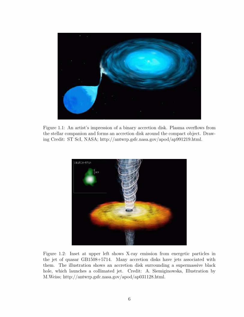
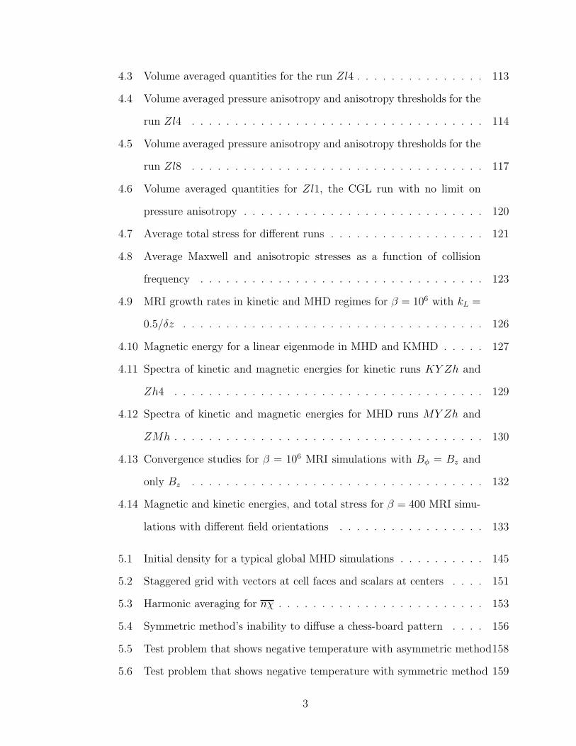
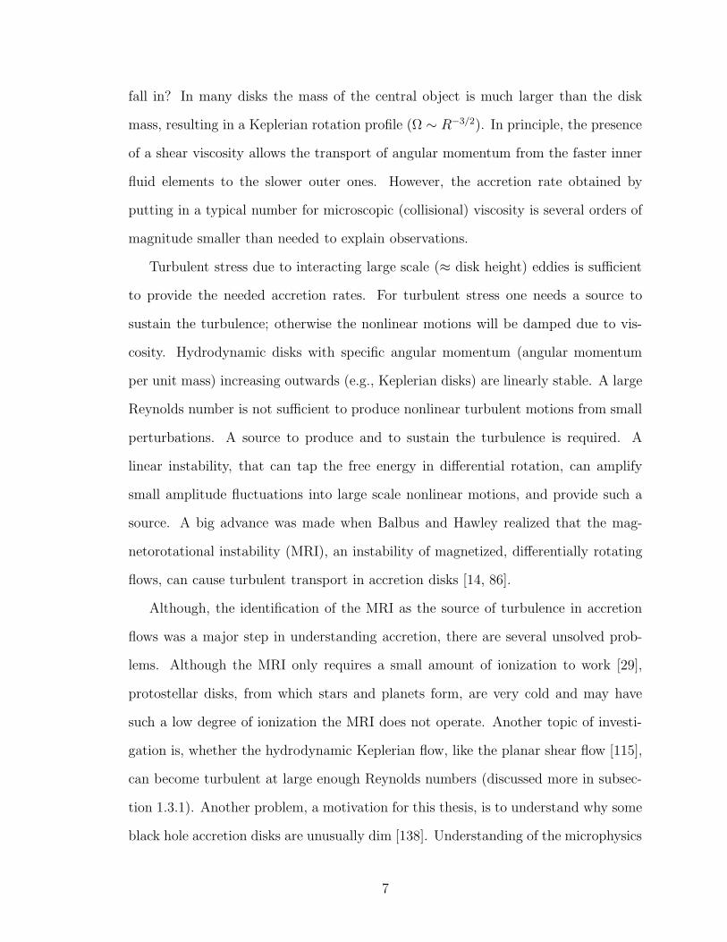
Figure 1.1: An artist’s impression of a binary accretion disk. Plasma overflows fromthe stellar companion and forms an accretion disk around the compact object. Draw-ing Credit: ST ScI, NASA; http://antwrp.gsfc.nasa.gov/apod/ap991219.html.

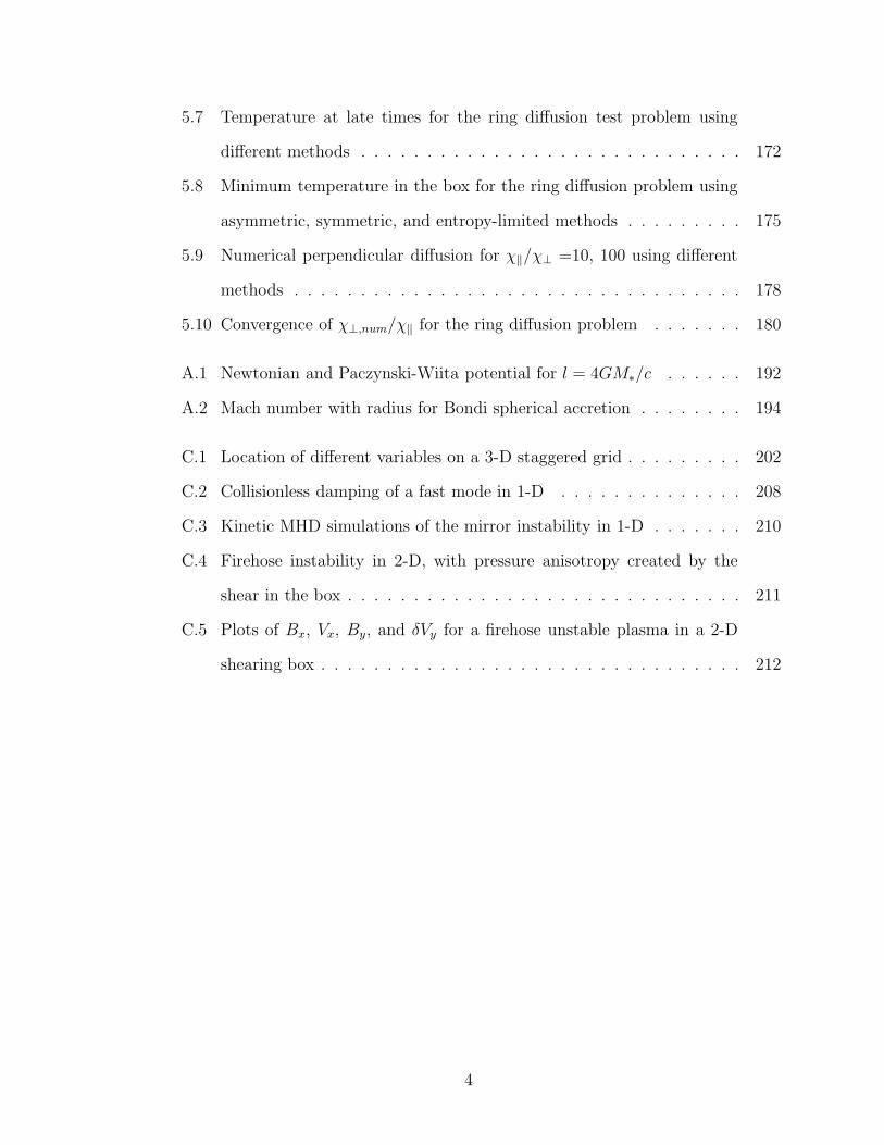
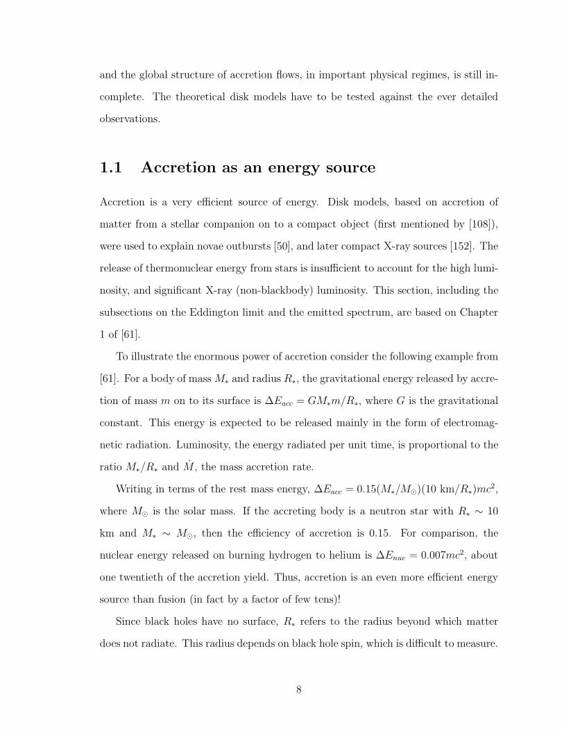
Figure 1.2: Inset at upper left shows X-ray emission from energetic particles inthe jet of quasar GB1508+5714. Many accretion disks have jets associated withthem. The illustration shows an accretion disk surrounding a supermassive blackhole, which launches a collimated jet. Credit: A. Siemiginowska, Illustration byM.Weiss; http://antwrp.gsfc.nasa.gov/apod/ap031128.html.

6

fall in? In many disks the mass of the central object is much larger than the disk

mass, resulting in a Keplerian rotation profile (Ω ∼ R−3/2). In principle, the presence

of a shear viscosity allows the transport of angular momentum from the faster inner

fluid elements to the slower outer ones. However, the accretion rate obtained by

putting in a typical number for microscopic (collisional) viscosity is several orders of

magnitude smaller than needed to explain observations.

Turbulent stress due to interacting large scale (≈ disk height) eddies is sufficient

to provide the needed accretion rates. For turbulent stress one needs a source to

sustain the turbulence; otherwise the nonlinear motions will be damped due to vis-

cosity. Hydrodynamic disks with specific angular momentum (angular momentum

per unit mass) increasing outwards (e.g., Keplerian disks) are linearly stable. A large

Reynolds number is not sufficient to produce nonlinear turbulent motions from small

perturbations. A source to produce and to sustain the turbulence is required. A

linear instability, that can tap the free energy in differential rotation, can amplify

small amplitude fluctuations into large scale nonlinear motions, and provide such a

source. A big advance was made when Balbus and Hawley realized that the mag-

netorotational instability (MRI), an instability of magnetized, differentially rotating

flows, can cause turbulent transport in accretion disks [14, 86].

Although, the identification of the MRI as the source of turbulence in accretion

flows was a major step in understanding accretion, there are several unsolved prob-

lems. Although the MRI only requires a small amount of ionization to work [29],

protostellar disks, from which stars and planets form, are very cold and may have

such a low degree of ionization the MRI does not operate. Another topic of investi-

gation is, whether the hydrodynamic Keplerian flow, like the planar shear flow [115],

can become turbulent at large enough Reynolds numbers (discussed more in subsec-

tion 1.3.1). Another problem, a motivation for this thesis, is to understand why some

black hole accretion disks are unusually dim [138]. Understanding of the microphysics

7

and the global structure of accretion flows, in important physical regimes, is still in-

complete. The theoretical disk models have to be tested against the ever detailed

observations.

1.1 Accretion as an energy source

Accretion is a very efficient source of energy. Disk models, based on accretion of

matter from a stellar companion on to a compact object (first mentioned by [108]),

were used to explain novae outbursts [50], and later compact X-ray sources [152]. The

release of thermonuclear energy from stars is insufficient to account for the high lumi-

nosity, and significant X-ray (non-blackbody) luminosity. This section, including the

subsections on the Eddington limit and the emitted spectrum, are based on Chapter

1 of [61].

To illustrate the enormous power of accretion consider the following example from

[61]. For a body of mass M∗ and radius R∗, the gravitational energy released by accre-

tion of mass m on to its surface is ∆Eacc = GM∗m/R∗, where G is the gravitational

constant. This energy is expected to be released mainly in the form of electromag-

netic radiation. Luminosity, the energy radiated per unit time, is proportional to the

ratio M∗/R∗ and M , the mass accretion rate.

Writing in terms of the rest mass energy, ∆Eacc = 0.15(M∗/M⊙)(10 km/R∗)mc2,

where M⊙ is the solar mass. If the accreting body is a neutron star with R∗ ∼ 10

km and M∗ ∼ M⊙, then the efficiency of accretion is 0.15. For comparison, the

nuclear energy released on burning hydrogen to helium is ∆Enuc = 0.007mc2, about

one twentieth of the accretion yield. Thus, accretion is an even more efficient energy

source than fusion (in fact by a factor of few tens)!

Since black holes have no surface, R∗ refers to the radius beyond which matter

does not radiate. This radius depends on black hole spin, which is difficult to measure.

8

Our ignorance of R∗ can be parameterized by an efficiency η, with ∆Eacc = ηmc2.

Relativistic calculations give an efficiency of 6% for a non-rotating Schwarzchild black

hole, and 42.3% for a maximally rotating Kerr black hole [133] (see Appendix A.1 for

a discussion of the efficiency of black hole accretion).

For a white dwarf with M∗ ∼M⊙, R∗ ∼ 109 cm, nuclear burning is more efficient

than accretion by factors 40−50. Although the efficiency for nuclear burning for white

dwarfs is much higher, in many cases the reaction tends to ‘run away’ to produce an

event of great brightness but short duration, a nova outburst, in which available

nuclear fuel is rapidly exhausted. For almost all of its lifetime no nuclear burning

occurs, and the white dwarf may derive its entire luminosity from accretion. Whether

accretion or nuclear fusion dominates depends on M , the accretion rate.

1.1.1 The Eddington limit

At high luminosity, the accretion flow is affected by the outward momentum trans-

ferred from radiation to the accreting matter by scattering and absorption. We derive

an upper limit on luminosity of an accretion disk by considering spherical, steady state

accretion. Assume the accreting matter to be fully ionized hydrogen plasma. If S

is radiant energy flux (erg cm−2 sec−1), and σT = 6.7 × 10−25cm2 is the electron

Thomson scattering cross section, the outward radial force is σTS/c. The effective

cross section can exceed σT if photons are absorbed by spectral lines. Because of the

charge neutrality of plasma, radiative force on electrons couples to protons. If L is

the luminosity of the accreting source, S = L/4πr2, net inward force on proton is

(GM∗mp −LσT /4πc)/r2. The limiting luminosity for which the radial force vanishes,

the Eddington limit, is LEdd = 4πGM∗mpc/σT∼= 1.38 × 1038(M∗/M⊙) erg s−1. At

greater luminosities, the radiation pressure will halt accretion. The Eddington limit

is a crude estimate of the upper limit on the steady state disk luminosity.

If all the kinetic energy of accretion is given up at the stellar surface, R∗, then

9

the luminosity is Lacc = GM∗M/R∗. For accretion powered objects, the Eddington

limit implies an upper limit on the accretion rate, M . MEdd = 4πR∗mpc/σT =

9.5 × 1011R∗ g s−1. The Eddington limit applies only for uniform, steady accretion;

e.g., photon bubble instability [6, 64, 30], a compressive instability of radiative disks

that opens up optically thin “holes” through which radiation can escape, can allow

for super-Eddington luminosity [193, 23].

1.1.2 The emitted spectrum

Order of magnitude estimates of spectral range of the emission from compact accreting

objects can be made. The continuum spectrum can be characterized by a temperature

Trad = hν/k of emitted radiation, where ν is the frequency of a typical photon. For

an accretion disk with luminosity Lacc, one can define a blackbody temperature as

Tb = (Lacc/4πR2∗σ)1/4, where σ is the Stefan-Boltzmann constant. Thermal temper-

ature, Tth, is defined as the temperature material would reach if its gravitational po-

tential energy is converted entirely into the thermal energy. For each proton-electron

pair accreted, the potential energy released is GM∗(mp +me)/R∗∼= GM∗mp/R∗, and

the thermal energy is 2 × (3/2)kT ; therefore Tth = GM∗mp/3kR∗. The virial tem-

perature, Tvir = Tth/2, is also used frequently. If the accretion flow is optically thick,

photons reach thermal equilibrium with the accreted material before leaking out to

the observer and Trad = Tb. Whereas, if accretion energy is converted directly into

radiation which escapes without further interaction (i.e., the intervening material is

optically thin), Trad = Tth. In general, the observed radiation temperature is expected

to lie between the two limits, Tb . Trad . Tth.

Applying these limits to a solar mass neutron star radiating at the Eddington limit

gives, 1 keV . hν . 50 MeV; similar results would hold for stellar mass black holes.

Thus we can expect the most luminous accreting neutron star and black hole binary

disks to appear as medium to hard X-ray emitters, and possibly as γ-ray sources.

10

Similarly for white dwarf accretion disks with M∗ = M⊙, R∗ = 109 cm, we obtain

6 eV . hν . 100 keV. Consequently, accreting white dwarfs should be optical, UV,

and possibly X-ray sources. Observations are mostly consistent with these estimates.

Nonthermal emission mechanisms also operate in disks. Examples are: syn-

chrotron emission by relativistic electrons spiraling around magnetic field lines and

inverse Compton up-scattering of photons by relativistic electrons. Line emission

because of electronic transition between energy levels provides a useful diagnostic of

density, temperature, and velocities in the emitting region.

Accretion disks, being efficient sources of energy, can be very luminous. Their

spectra are also very rich, extending all the way from radio to X-ray and γ-ray fre-

quencies. In order to interpret the radiative signatures, one needs to understand

transport and radiation processes in accretion disks.

1.2 Accretion disk phenomenology

Much of the phenomenology of accretion disks was developed in mid-1970’s when two

influential papers, by Shakura and Sunyaev [174], and Lynden-Bell and Pringle [121],

appeared. It was shown that in the presence of a shear viscosity, an infinitesimal mass

can carry away all the angular momentum of the inner fluid elements, facilitating mass

accretion [121, 153]. The structure (thick or thin) and radiation spectrum (luminous

or radiatively inefficient) of a disk depends mainly on the rate of matter inflow, M

[174]. Of course the overall luminosity and accretion time scale depends on M∗,the

mass of the central object.

A binary system consisting of a star and a compact object (black hole, neutron

star, or white dwarf) is likely to be very common in the Galaxy. The outflow of matter

from the star’s surface—the stellar wind—is significant (∼ 10−5M⊙ /yr) for massive

O-stars and Wolf-Rayet stars (M & 20M⊙). In binary systems, an additional strong

11

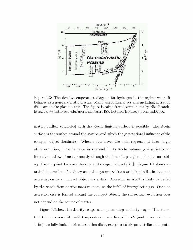
Figure 1.3: The density-temperature diagram for hydrogen in the regime where itbehaves as a non-relativistic plasma. Many astrophysical systems including accretiondisks are in the plasma state. The figure is taken from lecture notes by Niel Brandt,http://www.astro.psu.edu/users/niel/astro485/lectures/lecture08-overhead07.jpg

matter outflow connected with the Roche limiting surface is possible. The Roche

surface is the surface around the star beyond which the gravitational influence of the

compact object dominates. When a star leaves the main sequence at later stages

of its evolution, it can increase in size and fill its Roche volume, giving rise to an

intensive outflow of matter mostly through the inner Lagrangian point (an unstable

equilibrium point between the star and compact object) [61]. Figure 1.1 shows an

artist’s impression of a binary accretion system, with a star filling its Roche lobe and

accreting on to a compact object via a disk. Accretion in AGN is likely to be fed

by the winds from nearby massive stars, or the infall of intergalactic gas. Once an

accretion disk is formed around the compact object, the subsequent evolution does

not depend on the source of matter.

Figure 1.3 shows the density-temperature phase diagram for hydrogen. This shows

that the accretion disks with temperatures exceeding a few eV (and reasonable den-

sities) are fully ionized. Most accretion disks, except possibly protostellar and proto-

12

planetary disks, are sufficiently ionized for the plasma description to be valid [29, 16].

Even relatively cold gas disks may have enough ionization by cosmic rays [63], X-rays

[93], and radioactivity [168] to be sufficiently conducting for the MHD-like phenomena

to occur.

Magnetohydrodynamics (MHD) is a good approximation for a magnetized plasma

when the mean free path is much smaller than the scales of interest, e.g., in efficiently

radiating, dense, thin disks. This is not always the case; the radiatively inefficient

accretion flows (RIAFs), a motivation for this thesis, are believed to be collisionless

with the mean free path comparable to (or even larger than) the disk size (see Table

1.2 for plasma parameters in the Galactic center disk). Ideal MHD, where resistive

effects are negligible and the field is frozen into the plasma, is a good approximation

for large scale dynamics of almost all astrophysical plasmas; as the dynamical scales

are orders of magnitude larger than the resistive scale or the gyroradius scale. Even

with a large separation between the dynamical and resistive/viscous scales, dissipation

cannot be ignored—energy cascades from large scales to smaller scales, terminating

at the dissipative scales, where it is dissipated in shocks and reconnection. In the

inertial range of isotropic, homogeneous turbulence, energy dissipation rate balances

the rate at which energy is injected, independent of resistivity and viscosity [62, 27].

In rest of the section we closely follow the review article by Balbus and Hawley to

use the conservation of mass, energy, and angular momentum to derive the transport

properties of disks. The widely used α model for turbulent stress is introduced [174].

1.2.1 Governing equations

Following [16], the conservation of total energy in magnetohydrodynamics (MHD),

gives

∂

∂t

(

1

2ρV 2 +

3

2p+ ρΦ +

B2

8π

)

+ ∇· [ ] = −∇ · Frad, (1.1)

13

where ρ, V, p, B, and Φ are density, fluid velocity, pressure, magnetic field, and

gravitational potential, respectively. The term on the right represents radiative losses.

The conservative flux term ∇·[ ] consists of a dynamic contribution

v

(

1

2ρV 2 +

5

2p+ ρΦ

)

+B

4π× (V ×B), (1.2)

and a viscous contribution,

−ηV

(

∇V 2

2+

V

3∇ · V

)

+ηB

4π(∇× B) ×B, (1.3)

where, ηV is the microscopic kinematic shear viscosity, and ηB the microscopic re-

sistivity. Here we use a uniform, isotropic viscosity for simplicity. The Braginskii

viscosity is highly anisotropic as will be discussed later in the thesis. The dynamic

flux in Eq. (1.2) consists of an advective flux of kinetic and thermal energy (the first

term), and the Poynting flux of electromagnetic energy (the second term). The equa-

tion for angular momentum conservation in cylindrical, (R, φ, z), coordinate system

is given by

∂

∂t(ρRVφ) + ∇·R

[

ρVφV − Bφ

4πBp +

(

p+B2

8π

)

φ

]

− ∇·[

RηV

3(∇ · V)φ+ ηVR

2∇Vφ

R

]

= 0, (1.4)

where φ is the unit vector in the azimuthal direction, the subscript p refers to the

poloidal magnetic field components (the R and z components). In an accretion disk,

there is a net flux of energy and angular momentum in the radial direction, so the

divergence terms in Eqs. (1.1) and (1.4) are dominated by the radial derivatives of

radial fluxes.

14

1.2.2 Fluctuations

A fiducial disk system consists of a point mass potential situated at the center of

the disk, with the gas going around in a Keplerian rotation, Ω2 = GM∗/R3. The

fluctuation velocity is given by VR, δVφ = Vφ − RΩ, and Vz. When the azimuthal

velocity RΩ much exceeds the isothermal sound speed cs =√

p/ρ, the disk is thin;

the vertical structure is determined by hydrostatic balance, with the disk height scale

H = cs/Ω ≪ R. In this section we consider only thin disks because they are simpler,

for the vertical dynamics and pressure forces do not play a significant role. For thick

disks, where thermal forces are equally important and vertical motion is coupled to

the motion in plane, there is no universally accepted standard model [141, 160, 31].

The radial flux of angular momentum from Eq. (1.4) isR [ρVR(RΩ + δVφ) − BRBφ/4π].

Taking an azimuthal average, integrating over height, and averaging over a narrow

range ∆R in R, one obtains, ΣR[RΩ〈VR〉ρ + 〈VRδVφ − VARVAφ〉ρ], where the surface

density Σ =∫

ρdz, and for any X, 〈X〉ρ = 1/(2πΣ∆R)∫

XρdφdRdz. The notation

VAR, etc. denotes the Alfven velocity, VA = B/√

4πρ. The first term in the radial

angular momentum flux is the direct inflow of angular momentum due to radially

inward accretion of matter; the second term represents an outward component of flux

due to turbulent transport because of statistical correlations in the velocity and mag-

netic stress tensors [191]. The Rφ component of the stress, responsible for angular

momentum transport (see Eq. 1.4), is WRφ ≡ 〈VRδVφ − VARVAφ〉ρ.

In steady state, the angular momentum flux must be divergence free, and thus vary

as 1/R, i.e., ΣR2(RΩ〈VR〉ρ +WRφ) is independent of R. The condition of vanishing

stress at the inner edge (R∗) gives, Σ(ΩR〈Vr〉ρ + WRφ) = Σ∗Ω∗R∗〈Vr∗〉ρ(R∗/R)2.

Expressing in terms of the constant accretion rate, M = −2πRΣ〈VR〉ρ, leads to

−MRΩ/2π + ΣRWRφ = −MR2∗Ω∗/2πR. This gives an expression for the variation

15

of stress with radius as,

WRφ =MΩ

2πΣ

[

1 −(

R∗

R

)1/2]

. (1.5)

Keeping only the second order terms in the energy flux in Eq. (1.2), one gets

ρVR(Φ+R2Ω2/2+RΩδVφ)−(RΩ/4π)BRBφ. Upon averaging, height integrating, and

using the Keplerian potential Φ = −R2Ω2, energy flux becomes FE = MRΩ2/4π +

ΣRΩWRφ. Substituting for Ω and using Eq. (1.5) for the stress tensor, this reduces

to

FE =3GM∗M

4πR2

[

1 − 2

3

(

R∗

R

)1/2]

. (1.6)

The energy deposited by this flux is the source of disk’s luminosity. Minus the di-

vergence of the flux gives the disk surface emissivity (energy per unit area per unit

time), Q. Dividing by a factor of two for each side of the disk gives

Q =3GM∗M

8πR3

[

1 −(

R∗

R

)1/2]

. (1.7)

The Q− M relation depends on local energy conservation and is, as expected, inde-

pendent of the form of the stress tensor (see [174, 153]). Eliminating M between Eqs.

(1.5) and (1.7) yields

Q =3

4ΣΩWRφ =

3

4ΣΩ〈VRδVφ − VARVAφ〉ρ, (1.8)

a kind of fluctuation-dissipation relation for accretion disks [13]. From Eqs. (1.5)

and (1.8), it is clear that the correlation of velocity (and magnetic field) fluctuation

components is responsible for much of the disk transport and luminosity.

Above discussion is valid only for a cold, thin disk where pressure can be ignored.

For a radiatively inefficient, hot, thick disk the pressure term (5/2)pVR should be

16

included in the radial energy flux; ∇·FE ≈ 0 in absence of radiation, and the gravita-

tional energy released from accretion is converted into thermal and kinetic energies.

Total luminosity emitted fromR∗ toR is, L(R∗ < R) = 2π[R∗FE(R∗)−RFE(R)] =

(GM∗M/2R∗)[1−3R/R∗+(R∗/R)3/2]. In the limit R → ∞, L = GM∗M/2R∗, which

shows that half the binding energy of the innermost orbit is converted to radiation.

The other half is retained as kinetic energy. The fate of the residual energy depends

on the nature of central accretor. If a stellar surface is present, remaining energy will

be radiated in a boundary layer; if the central object is a black hole, the energy may

be swallowed and lost.

1.2.3 α disk models

Although the relationship between disk’s surface emissivity Q and the mass accretion

rate M is independent of stress tensor, most other relations involve a dependence on

WRφ. Recognizing the central importance of WRφ and its computational inaccessi-

bility, Shakura and Sunyaev [174] suggested a natural scaling for the stress tensor,

WRφ = αc2s, where α . 1 is a parameter. The idea behind the α prescription is that

the turbulent velocities, whose correlation determines WRφ, are limited by the sound

speed cs, as supersonic velocities will be quickly dissipated in shocks. The α formal-

ism bypasses the thorny issue of disk turbulence, and can be thought as a closure for

the stress tensor. The α formalism can be thought of as equivalent to a “turbulent

viscosity”

νt = αcsH (1.9)

that is similar to microscopic viscosity in Navier Stokes equation. The role of random

particle velocity is played by cs, and the scale height H is the effective mean free path

(eddy size). This is a closure based on plausibility arguments and is not rigorous

like the Chapman-Enskog procedure [47]. The α formalism is the basis of much of

17

observationally driven disk phenomenology. The radial dependence of various phys-

ical quantities, like temperature, density, height, etc., can be obtained in terms of

parameters M and α [61].

1.3 MRI: the source of disk turbulence

A breakthrough occurred when Balbus and Hawley proposed the magnetorotational

instability (MRI), an instability of differentially rotating flows, as the source for tur-

bulence and transport in accretion disks [14]. Before this, a robust mechanism to

sustain turbulent angular momentum transport in accretion disks was unknown. Al-

though the instability was described in its global form for magnetized Couette flow

by Velikhov [197] and Chandrasekhar [44], its importance for accretion disks was not

recognized. In his classic book [45], Chandrasekhar points out the essential feature

of the MRI, “in the limit of zero magnetic field, a sufficient condition for stability

is that the angular speed, |Ω|, is a monotonic increasing function of r. At the same

time, any adverse gradient of angular velocity can be stabilized by a magnetic field

of sufficient strength.”

Both local [86] and global [5, 81, 188] numerical simulations have confirmed that

the MRI can amplify small perturbations to nonlinear turbulent motions. Correla-

tions between the radial and azimuthal fields results in a sustained turbulent stress

corresponding to α ≡WRφ/p ∼ 0.001 − 0.5, enough to account for typical disk lumi-

nosities. Next, we discuss the inadequacy of the hydrodynamic models, followed by

the linear and nonlinear characteristics of the MRI.

1.3.1 Insufficiency of hydrodynamics

In the Boussinesq approximation (∇ · V = 0 in the equation of motion), if we ignore

pressure, then a fluid element disturbed slightly from its Keplerian orbit will execute

18

retrograde epicycles at a frequency κ (κ2 ≡ 1R3

d(R4Ω2)dR

), as seen by an observer in

an unperturbed Keplerian orbit. The criterion for local linear stability is simply

κ > 0, i.e., specific angular momentum increases outwards, the Rayleigh criterion.1

Therefore, a Keplerian disk with specific angular momentum R2Ω ∼ R1/2, increasing

outwards is linearly stable, unable to produce (and sustain) nonlinear turbulent stress.

A rotating shear flow is different from a planar shear flow because of the coriolis

force. Coriolis force is responsible for stable epicyclic oscillations in Keplerian flows,

whereas planar shear flows are marginally stable in the linear regime. Nonlinear

local shearing box simulations show that while planar shear flows can be nonlin-

early unstable and become turbulent even at relatively small Reynolds numbers [21],

103 − 104 (orders of magnitude smaller than the true Reynolds number for disks),

Keplerian disks are nonlinearly stable and give no turbulence over the same range of

Reynolds numbers [17, 85]. This is because stable epicycles prevent nonlinear insta-

bilities to develop in Keplerian flows. Whether turbulence and transport can occur

in hydrodynamic Keplerian flows, is still not universally agreed. There are exper-

imental claims that the Keplerian disks are nonlinearly unstable [164], but recent

experiments, with more carefully controlled boundary conditions (especially Eckman

flows), which directly measure the Reynolds stress, show otherwise [39]. Also, there is

some recent work on transient amplification in the linear regime, that can give rise to

nonlinear amplitudes (and maybe turbulence) in hydrodynamic differentially rotating

flows [42, 2, 195].

Convective turbulence was also proposed as a source of enhanced shear viscosity

[118]. Convection is believed to arise from heating due to energy dissipated in the

disk midplane. The hope was that somehow convective blobs can cause nonlinear cor-

relations to produce non-vanishing stress. However, the linear analysis of convective

instability in Keplerian flows gives a wrong sign of stress [166], with inward trans-

1The Rayleigh criterion applies only for axisymmetric disturbances.

19

port of angular momentum. Three dimensional simulations of convectively unstable

disk show very small angular momentum transport (α ∼ −10−4), and in the oppo-

site direction [183]. None of the local hydrodynamic mechanisms to date are able to

give sufficient angular momentum transport.2 This launches us to the study of the

dramatic effect of magnetic fields on accretion disk stability.

1.3.2 MHD accretion disks: Linear analysis

The ideal MHD equations are

∂ρ

∂t+ ∇ · (ρV) = 0, (1.10)

ρ∂V

∂t+ ρ (V · ∇)V =

(∇× B) × B

4π−∇p+ Fg, (1.11)

∂B

∂t= ∇× (V × B) , (1.12)

∂e

∂t+ ∇ · (eV) = −p∇ · V, (1.13)

where, Fg is the gravitational force, and e = p/(γ− 1) relates internal energy density

and pressure (γ = 5/3 in a 3-D non-relativistic plasma). Making B = 0 in the MHD

equations gives the hydrodynamic equations.

WKB analysis in a Keplerian disk

The linear response of a Keplerian hydrodynamic flow is stable epicyclic motion,

however, addition of weak magnetic fields renders it unstable. Before considering

Keplerian flows, it is useful to study waves in a homogeneous, non-rotating equilib-

rium. Linear waves in MHD and hydrodynamics are quite different. MHD is richer

in waves with fast, Alfven, and slow modes, compared to hydrodynamics with only

an isotropically propagating sound wave [111]. As the name suggests, the fast mode

2Global modes like Papaloizou-Pringle instability [146, 72], and spiral shocks can in principlecause turbulence and transport, however, their role as a universal transport mechanism for Kepleriandisks is not clear [16].

20

has the fastest phase speed and propagates isotropically. The Alfven mode is inter-

mediate with propagation along the field lines, and the slow mode with the smallest

phase speed also propagates along the field lines. In addition to these, there is a non-

propagating entropy mode with anticorrelated density and temperature fluctuations.

Consider a differentially rotating disk threaded by a magnetic field with a vertical

component Bz and an azimuthal component Bφ. Consider WKB perturbations of the

form exp i(k · r− ωt), kR≫ 1. Notation is the standard one: k is the wave vector, r

the position vector, ω the angular frequency, and t the time. Linear perturbations are

denoted by δ. Only a vertical wave number is considered, k = kz. The local linear

equations are

−ωδρρ

+ kδVz = 0, (1.14)

−iωδVR − 2ΩδVφ − ikBz

4πρδBR = 0, (1.15)

−iωδVφ +κ2

2ΩδVR − i

kBz

4πρδBφ = 0, (1.16)

−ωδVz + k

(

δp

ρ+BφδBφ

4πρ

)

= 0, (1.17)

−ωδBR = kBzδVR, (1.18)

−iωδBφ = δBRdΩ

d lnR+ ikBzδVφ −BφikδVz, (1.19)

δBz = 0, (1.20)

δp

p=

5

3

δρ

ρ. (1.21)

The resulting dispersion relation is (Eq. (99) in [16])

[ω2 − (k · VA)2][ω4 − k2ω2(a2 + V 2A) + (k ·VA)2k2a2]

−[

κ2ω4 − ω2

(

k2κ2(a2 + V 2Aφ) + (k · VA)2 dΩ2

d lnR

)]

− k2a2(k · VA)2 dΩ2

d lnR= 0, (1.22)

21

where a2 = (5/3)P/ρ, VA = B/√

4πρ. Only the first term in the dispersion relation,

Eq. (1.22), is non-zero in the non-rotating limit; the roots of the dispersion relation

correspond to the fast, Alfven, and slow modes.

The effect of Keplerian rotation on the three MHD modes is shown in Fig. (15) of

Balbus and Hawley’s review article [16], with ω2 plotted as a function of Ω2 (also see

Figure 3.4). It shows that ω2 becomes negative for the slow mode when dΩ2/d lnR >

(k · VA)2, i.e., slow modes becomes unstable. This destabilized MHD slow mode in

differentially rotating flows is the MRI. For a fixed wave number there is an upper

limit on the field strength for the MRI to exist, i.e., it is a weak field instability.

Spring model of the MRI

A simple physical description of the MRI, based on the spring model of Balbus and

Hawley, is presented; the discussion closely follows [16]. It is useful to study the

instability in the Boussinesq limit, where fast waves are eliminated. The simplest

model to think is of axisymmetric perturbations on uniform vertical magnetic field

in a Keplerian disk. If a fluid element is displaced from its circular orbit by ξ, with

a spatial dependence eikz, induction equation leads to δB = ikBξ. Magnetic tension

force is then ikBδB/4πρ = −(k · VA)2ξ. In an incompressible, pressure free limit,

the equations of motion become

ξR − 2Ωξφ = −(

dΩ2

d lnR+ (k · VA)2

)

ξR, (1.23)

ξφ + 2ΩξR = −(k ·VA)2ξφ. (1.24)

As before, 2Ω and dΩ2/d lnR terms represent coriolis and tidal forces, respectively.

These equations also describe two orbiting point masses connected with a spring of

spring constant (k · VA)2.

Consider two point masses, initially at the same orbital location, displaced slightly

22

M∗

mi

mi

mo

mo

T

T

T

φ

RR

z

H

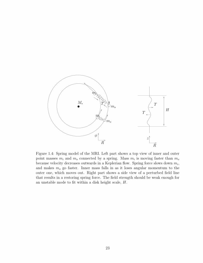
Figure 1.4: Spring model of the MRI. Left part shows a top view of inner and outerpoint masses mi and mo connected by a spring. Mass mi is moving faster than mo

because velocity decreases outwards in a Keplerian flow. Spring force slows down mi,and makes mo go faster. Inner mass falls in as it loses angular momentum to theouter one, which moves out. Right part shows a side view of a perturbed field linethat results in a restoring spring force. The field strength should be weak enough foran unstable mode to fit within a disk height scale, H .

23

in the radial direction, as shown in Figure 1.4. The inner mass mi at radius Ri is

connected via a spring to outer mass mo at Ro. In a Keplerian disk, the inner mass

rotates faster than the outer one. In the absence of a spring both execute stable

epicycles. However, the spring stretches and builds up a tension T . T pulls backward

on mi and forward on mo. Thus, mi slows down and loses angular momentum to mo

which gains speed. This means that the slower mi (compared to the local Keplerian

velocity) cannot remain in orbit at Ri and must drop to a yet lower orbit. Similarly,

mo acquire too much angular momentum to stay at Ro and must move outwards.

The separation widens, the spring stretches yet more, T goes up, and the process

runs away. This is the essence of weak field instability in differentially rotating flows.

The presence of other field components does not affect this picture, as by selecting

k = kzz we have ensured that only vertical field couples dynamically. It is very crucial

that the spring be weak; if spring is very stiff, there are many stable vibrations in

an orbital time and no net transport of angular momentum. The right side of Eq.

(1.23) reproduces the stability criterion for the slow mode, (k · VA)2 > −dΩ2/d lnR.

One can always choose a small enough k to make a Keplerian disk unstable. Thus,

the necessary and sufficient condition for the stability of a magnetized differentially

rotating disk is dΩ2/d lnR > 0.

Just how large a wavelength is permitted? In order for the WKB approximation

to be valid, at least a half wavelength needs to fit in the box height H . The stability

criterion for a Keplerian disk becomes V 2A > H2

π2

dΩ2

d ln R∼ (6/π2)c2s, i.e., the Alfven speed

must significantly exceed the sound speed, if all the modes in a disk thickness are to

be stable. The MRI is called a weak field instability because it requires pressure

to exceed magnetic energy (β = 8πp/B2 & 1). It is interesting to note that there

is no lower limit on the strength of the magnetic field for the instability to exist if

dissipation scales are arbitrarily small [106].

The dispersion relation from Eqs. (1.23) and (1.24), on assuming ξ ∼ exp(−iωt),

24

is

ω4 − ω2[κ2 + 2(k · VA)2] + (k ·VA)2

(

(k · VA)2 +dΩ2

d lnR

)

= 0, (1.25)

which is precisely the a→ ∞ Boussinesq limit of Eq. (1.22). Eq. (1.25) is a quadratic

in ω2 which can be solved easily. The fastest growth rate for a Keplerian disk is

γmax = (3/4)Ω, and occurs at (k ·VA)max = (√

15/4)Ω. This is a very fast instability

that would cause amplification by ∼ 104 in energy, per orbit. The instability is

very robust, independent of the magnetic field orientation. In presence of a toroidal

field the MRI is non-axisymmetric for the perturbations to couple to the field [15].

Nonlinear correlations resulting from this instability can provide a sizeable stress to

explain fast angular momentum transport in disks, as we see in the next subsection.

1.3.3 MHD accretion disks: Nonlinear simulations

Tremendous progress has been made in the understanding of growth and saturation of

the MRI. Numerical studies started with unstratified local shearing box simulations

[82, 86] using the ZEUS MHD code [185, 186]. In the shearing box limit, equations

are written in a frame rotating with the mean flow. There is shear in a Keplerian box

with dΩ/d lnR = −3/2. Boundary conditions are periodic in y- (azimuthal) and z−

(vertical) directions, and shearing periodic in x- (radial direction).3

Shearing box simulations start with a random white noise imposed on an initial

equilibrium. In simulations with a net vertical flux, magnetic energy increases expo-

nentially until the channel solution (the nonlinear form of the fastest growing mode

with kzVAz/Ω ∼ 1) becomes unstable to secondary Kelvin-Helmholtz type instabili-

ties [75]. Magnetic energy increases by several orders of magnitude before secondary

instabilities break the channel solutions into turbulence. Magnetic energy saturates at

3Shearing periodic means that periodic boundary conditions are applied after a time dependentremap in y- direction at the x- boundaries [86, 16]. There is a jump of −(3/2)ΩLx in Vy between theinner and outer radial faces to take differential rotation into account. There are similarities betweenthis and the boundary conditions used in fusion energy research to handle sheared magnetic fieldsin flux-tube simulations of turbulence [49, 77, 22].

25

0 5 10 15 20

10−10

10−5

100

orbits

<B2/8πp0>

<−BxB

y/4πp

0>

<ρVxδV

y/p

0>

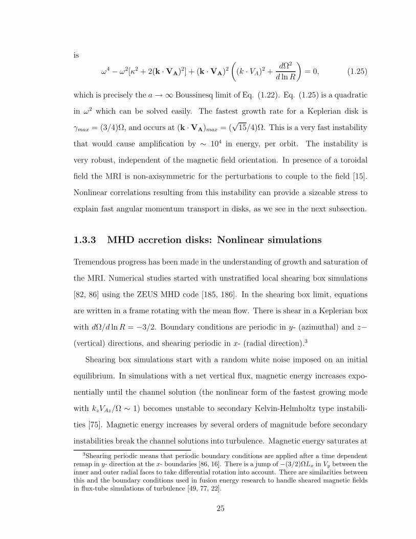
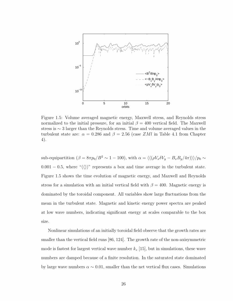
Figure 1.5: Volume averaged magnetic energy, Maxwell stress, and Reynolds stressnormalized to the initial pressure, for an initial β = 400 vertical field. The Maxwellstress is ∼ 3 larger than the Reynolds stress. Time and volume averaged values in theturbulent state are: α = 0.286 and β = 2.56 (case ZMl in Table 4.1 from Chapter4).

sub-equipartition (β = 8πp0/B2 ∼ 1 − 100), with α = 〈〈(ρVxδVy −BxBy/4π)〉〉/p0 ∼

0.001 − 0.5, where “〈〈〉〉” represents a box and time average in the turbulent state.

Figure 1.5 shows the time evolution of magnetic energy, and Maxwell and Reynolds

stress for a simulation with an initial vertical field with β = 400. Magnetic energy is

dominated by the toroidal component. All variables show large fluctuations from the

mean in the turbulent state. Magnetic and kinetic energy power spectra are peaked

at low wave numbers, indicating significant energy at scales comparable to the box

size.

Nonlinear simulations of an initially toroidal field observe that the growth rates are

smaller than the vertical field runs [86, 124]. The growth rate of the non-axisymmetric

mode is fastest for largest vertical wave number kz [15], but in simulations, these wave

numbers are damped because of a finite resolution. In the saturated state dominated

by large wave numbers α ∼ 0.01, smaller than the net vertical flux cases. Simulations

26

with no net flux, 〈B〉 = 0, also result in sustained MHD turbulence and transport

at large scales. However, both magnetic energy and turbulent stress are smaller by

a factor of 10 − 100 compared with the net vertical field case [87]. Toroidal fields

and the Maxwell stress dominate the other components, irrespective of the initial

field configuration. Total stress is roughly proportional to the magnetic energy for all

cases.

Stratified shearing boxes with vertical gravity were simulated to closely model a

real accretion disk in the local limit [38, 184]. Vertical stratification allow the pos-

sibility of vertical motions driven by magnetic buoyancy. Stratified simulations are

not very different from the unstratified ones because the Mach number (the ratio of

fluid velocity and sound speed, V/cs) is much less than unity for MRI turbulence.

This ensures that the MRI timescale (1/Ω = H/cs) is much faster than the time scale

for buoyant motions at large scales (H/V ). Results are similar for the adiabatic and

isothermal equations of state [184]. While the R − φ dynamics is dominated by the

MRI, vertical stratification can result in significant mixing in the z− direction. Strat-

ified simulations show the eventual emergence of a magnetically dominated corona

stable to the MRI because of buoyantly rising magnetic fields [132]. It is reassuring

that irrespective of initial fields geometry, equation of state, boundary conditions,

vertical stratification, numerical methods, etc., MHD turbulence and efficient trans-

port of angular momentum always ensues. But the question of the exact saturation

level and its dependence on physical and numerical parameters, such as net verti-

cal flux, box size, or dissipation mechanisms, remain a topic of continued research

[87, 167, 198, 28, 150].

Local shearing boxes have been used extensively to understand MRI turbulence in

presence of other physical effects, e.g., resistivity [59], ambipolar diffusion [88], Hall

effect [169], radiation and the photon bubble instability [194, 193], and the thermal

instability [151].

27

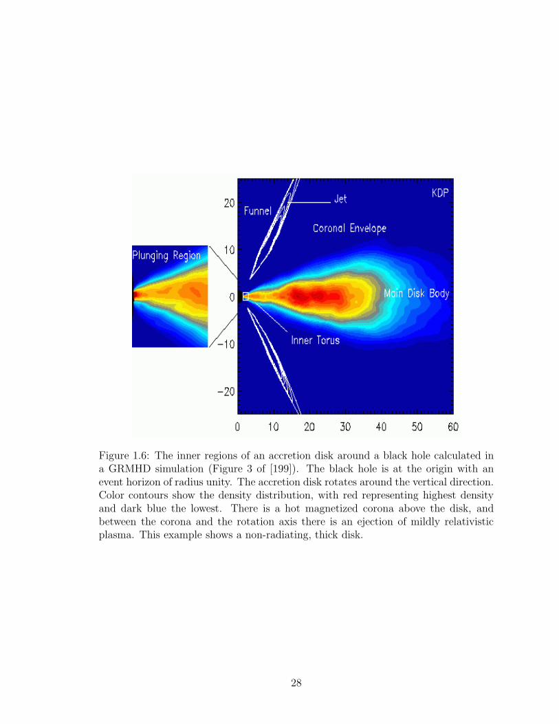
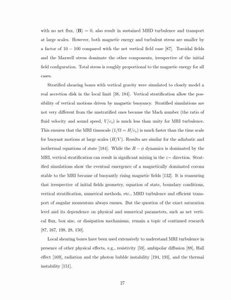
Figure 1.6: The inner regions of an accretion disk around a black hole calculated ina GRMHD simulation (Figure 3 of [199]). The black hole is at the origin with anevent horizon of radius unity. The accretion disk rotates around the vertical direction.Color contours show the density distribution, with red representing highest densityand dark blue the lowest. There is a hot magnetized corona above the disk, andbetween the corona and the rotation axis there is an ejection of mildly relativisticplasma. This example shows a non-radiating, thick disk.

28

The effect of MRI turbulence was first observed in global 2-D MHD simulations

of Shibata and Uchida with a net vertical flux [178], but the reason for the disrup-

tion of the flow was not understood. Starting from the 2-D simulations [178, 187],

tremendous progress in computer hardware and algorithms has made it possible to

simulate realistic disks around rotating Kerr black holes with general relativistic MHD

(GRMHD) in 3-D [199, 105]. Figure 1.6 shows the structure of a disk from a GRMHD

simulation [199]. In addition to the efficient angular momentum transport in disks

due to the MRI, global simulations allows one to study angular momentum extrac-

tion by global mechanisms such as magnetic braking and winds [33], and extraction of

black hole spin energy in form of jets [34, 128, 102, 105]. Global simulations have also

been used to understand the structure of thick disks in radiatively inefficient accretion

flows (RIAFs, see Fig. 1.6), the subject of the next section [189, 188, 83, 155].

1.4 Radiatively inefficient accretion flows

This section borrows heavily from an unpublished document on the motivation for

studying radiatively inefficient accretion flow (RIAF) regimes, by E. Quataert. There

is growing observational evidence for the presence of supermassive black holes (SMBHs)

in galactic nuclei. High resolution imaging of the stellar orbits around a dark object

in the Galactic center, using adaptive optics, provides a compelling evidence for a

4.1 ± 0.6 × 106M⊙M⊙ SMBH [171, 71] (see Figure 1.7). Very large baseline interfer-

ometry (VLBI) observations of water masers in NGC 4258 show gas in a Keplerian

orbit about a SMBH [134]. More generally, stellar motions and radiation from hot

gas in the central regions of nearby galaxies have shown that SMBHs are present in

nearly every galaxy with a bulge component [122, 70, 58]. 4

One of the puzzles about many SMBHs is their extreme low luminosity, despite

their gas rich environments. In contrast, the Active Galactic nuclei (e.g., quasars),

4The bulge component of a galaxy is the central roughly spherical region with old stars.

29

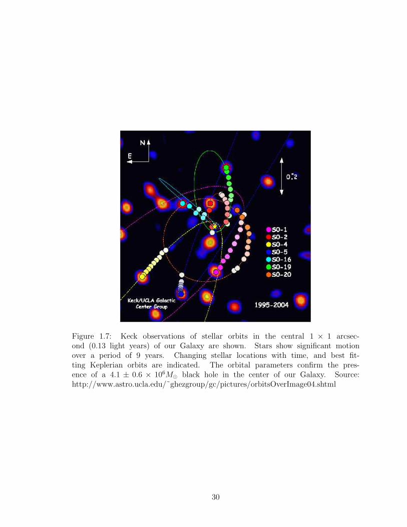
Figure 1.7: Keck observations of stellar orbits in the central 1 × 1 arcsec-ond (0.13 light years) of our Galaxy are shown. Stars show significant motionover a period of 9 years. Changing stellar locations with time, and best fit-ting Keplerian orbits are indicated. The orbital parameters confirm the pres-ence of a 4.1 ± 0.6 × 106M⊙ black hole in the center of our Galaxy. Source:http://www.astro.ucla.edu/˜ghezgroup/gc/pictures/orbitsOverImage04.shtml

30

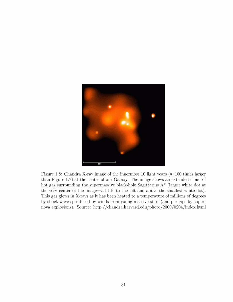
Figure 1.8: Chandra X-ray image of the innermost 10 light years (≈ 100 times largerthan Figure 1.7) at the center of our Galaxy. The image shows an extended cloud ofhot gas surrounding the supermassive black-hole Sagittarius A* (larger white dot atthe very center of the image—a little to the left and above the smallest white dot).This gas glows in X-rays as it has been heated to a temperature of millions of degreesby shock waves produced by winds from young massive stars (and perhaps by super-nova explosions). Source: http://chandra.harvard.edu/photo/2000/0204/index.html

31

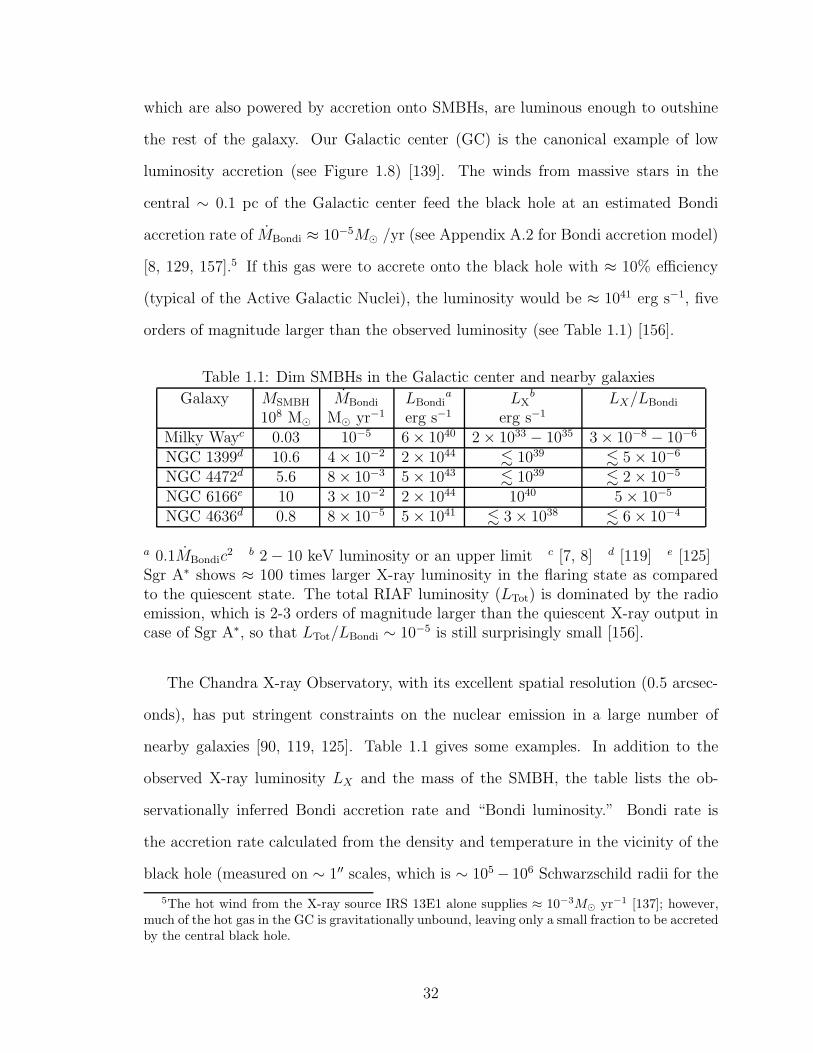
which are also powered by accretion onto SMBHs, are luminous enough to outshine

the rest of the galaxy. Our Galactic center (GC) is the canonical example of low

luminosity accretion (see Figure 1.8) [139]. The winds from massive stars in the

central ∼ 0.1 pc of the Galactic center feed the black hole at an estimated Bondi

accretion rate of MBondi ≈ 10−5M⊙ /yr (see Appendix A.2 for Bondi accretion model)

[8, 129, 157].5 If this gas were to accrete onto the black hole with ≈ 10% efficiency

(typical of the Active Galactic Nuclei), the luminosity would be ≈ 1041 erg s−1, five

orders of magnitude larger than the observed luminosity (see Table 1.1) [156].

Table 1.1: Dim SMBHs in the Galactic center and nearby galaxies

Galaxy MSMBH MBondi LBondia LX

b LX/LBondi

108 M⊙ M⊙ yr−1 erg s−1 erg s−1

Milky Wayc 0.03 10−5 6 × 1040 2 × 1033 − 1035 3 × 10−8 − 10−6

NGC 1399d 10.6 4 × 10−2 2 × 1044 . 1039 . 5 × 10−6

NGC 4472d 5.6 8 × 10−3 5 × 1043 . 1039 . 2 × 10−5

NGC 6166e 10 3 × 10−2 2 × 1044 1040 5 × 10−5

NGC 4636d 0.8 8 × 10−5 5 × 1041 . 3 × 1038 . 6 × 10−4

a 0.1MBondic2 b 2 − 10 keV luminosity or an upper limit c [7, 8] d [119] e [125]

Sgr A∗ shows ≈ 100 times larger X-ray luminosity in the flaring state as comparedto the quiescent state. The total RIAF luminosity (LTot) is dominated by the radioemission, which is 2-3 orders of magnitude larger than the quiescent X-ray output incase of Sgr A∗, so that LTot/LBondi ∼ 10−5 is still surprisingly small [156].

The Chandra X-ray Observatory, with its excellent spatial resolution (0.5 arcsec-

onds), has put stringent constraints on the nuclear emission in a large number of

nearby galaxies [90, 119, 125]. Table 1.1 gives some examples. In addition to the

observed X-ray luminosity LX and the mass of the SMBH, the table lists the ob-

servationally inferred Bondi accretion rate and “Bondi luminosity.” Bondi rate is

the accretion rate calculated from the density and temperature in the vicinity of the

black hole (measured on ∼ 1′′ scales, which is ∼ 105 − 106 Schwarzschild radii for the

5The hot wind from the X-ray source IRS 13E1 alone supplies ≈ 10−3M⊙ yr−1 [137]; however,much of the hot gas in the GC is gravitationally unbound, leaving only a small fraction to be accretedby the central black hole.

32

systems in Table 1.1), and assuming spherical hydrodynamic accretion (see Appendix

A.2). Bondi luminosity is the luminosity if the ambient gas accretes onto the SMBH

at the Bondi rate and emits with ≈ 10% efficiency. For all cases in Table 1.1, LX

is much less than the Bondi luminosity (which is orders of magnitude smaller than

the Eddington limit for these systems). Thus, the observed luminosities are orders of

magnitude smaller than simple theoretical predictions. Moreover, these discrepancies

are not unique to X-ray observations, but are present in high resolution observations

from the radio to the gamma-rays [89].

1.4.1 RIAF models

With compelling evidence for low luminosity SMBHs in the Galactic center and nearby

galaxies, one needs to account for their extreme dimness. The explanation for their

low luminosity must lie in how the surrounding gas accretes onto the central black

hole. The standard accretion disk model is that of a geometrically thin, optically

thick disk [174], applied extensively to luminous accreting sources in X-ray binaries

and AGN [103, 56]. Low luminosity disks are fundamentally different; radiatively

inefficient disks retain most of the accretion energy as thermal motion and puff up

to become thick. Also, RIAFs show no significant black body component in their

spectra in infrared-UV [114, 89, 161]; this emission is seen in luminous sources such

as Seyferts and quasars [103]. Most low luminosity disk models have appealed to

modes other than thin disks. Accretion disks where very little of the gravitational

potential energy of the accreting gas is radiated away is referred to as radiatively

inefficient accretion flows (RIAFs).

The plasma in RIAFs is hot and dilute because the gravitational energy released

from accretion is stored as thermal energy. Because of the low densities and high

temperatures, Coulomb collisions are inefficient at exchanging energy between the

electrons and protons (see Table 1.2). If protons and electrons are heated to their

33

respective virial temperatures without exchanging energy, then protons will be hotter

than electrons by their mass ratio mp/me ≈ 2000. But the temperatures depend

on how energy released from accretion is dissipated into electrons and ions, which

remains poorly understood. Most RIAF models assume that protons (∼ 1012 K) are

much hotter than the electrons (∼ 1010 − 1012 K) [156]. The electron temperature is

not well constrained but crucial as it determines the radiation that we see. The hot

RIAFs are thus very different from the thin accretion disks, which are much cooler

(∼ 105−106 K) and denser. In addition, because of the different physical conditions in

the accretion flow, thin disk and RIAF models predict very different multiwavelength

spectra (e.g., RIAFs are optically thin and do not produce blackbody emission).

Two ways to make a disk radiatively inefficient are: 1) energy released from ac-

cretion at Bondi rate is channeled preferentially into poorly radiating ions, which

are eventually swallowed (with their energy) by the hole; and 2) instead of accreting

all the available gas supply, processes like winds and outflows, and convection can

constrict the net accretion (M ≪ MBondi) onto the black hole.

The original RIAF models by Ichimaru (1977) and Rees et. al. (1982; the “ion

torus” model) [92, 163] were based on the first approach. These models were revived

in the 1990s, and extensively applied to observed systems, under the name advection-

dominated accretion flows (ADAFs), by Narayan, Abramowicz, and others [141, 142,

1]. In ADAF models, the gas accretes at about the Bondi rate, but the radiative

efficiency is ≪ 10%, providing a possible explanation for the very low luminosity

of most galactic nuclei [163, 57]. The radiative efficiency is very low because it is

assumed that the electrons, which produce the radiation we see, are much colder

than the ions which are advected (with their thermal energy) on to the hole. Thus,

instead of energy release in the form of radiation like in the cool, thin disks, energy

is lost forever to the black hole in ADAF models.

The past few years have seen new steps in the theoretical understanding of RIAFs.

34

In particular, hydrodynamic and MHD numerical simulations of RIAFs have been

performed [189, 94, 188, 84, 83, 95, 149, 154, 155]. The hydrodynamic simulations

based on α model for stress (e.g., [189, 94, 154]) found that convection can stall

accretion, with density varying like ρ ∼ r−1/2 with radius, as compared to a steeper ∼

r−3/2 dependence in ADAFs and Bondi accretion (see [141] and Appendix A.2). These

simulations motivated analytical self-similar models known as convectively dominated

accretion flows (CDAFs). The reason for a less steep dependence of density on radius

is that the mass accretion rate in CDAFs decreases as we move in towards the black

hole, M/MADAF ∼ (r/racc). The low luminosity in CDAFs is not because of low

efficiency of accretion (η ∼ 0.1), but because of the reduction of mass accretion due to

convection. In global MHD simulations strong magnetic fields (β . 10) are generated

by MHD turbulence driven by the MRI, and convection is unimportant [188, 84,

83, 95, 149, 155]. Numerical simulations by different groups (using different codes

and boundary conditions) lead to the same conclusion—magnetically driven outflows

prevent most of the mass supplied at outer regions to accrete. Outflows are natural

outcome of hot RIAFs and have been incorporated in theoretical models to account for

low accretion rates [141, 31, 32]; this adiabatic inflow-outflow solution (ADIOS) model

also predicts a smaller accretion rate in the inner regions, (M/MADAF ∼ (r/racc)p,

with 0 ≤ p ≤ 1), and a gentle dependence of density on radius (ρ ∼ r−3/2+p) compared

to an ADAF.

The ADIOS/CDAF models look very different from ADAF models; very little

of the mass supplied at large radii actually accretes into the black holes. The ac-

cretion rate can be smaller than the Bondi estimate (e.g., Table 1.1) by a factor of

∼ Racc/RS ∼ 105, where RS and Racc are the inner (∼ 2GM∗/c2, the Schwarzschild

radius) and the outer (∼ racc = 2GM∗/a2, the Bondi accretion radius) radii of the

accretion flow. This very low accretion rate may explain the low luminosity of most

galactic nuclei.

35

1.4.2 The Galactic center

Following Baganoff et al. [8], we apply the models discussed in the previous subsection

to Sgr A∗, the RIAF in the Galactic center (GC). The high resolution Chandra X-ray

observations have enabled the detection of X-rays in the vicinity of Sgr A∗, unpolluted

by the emission from other X-ray sources in the region [8]. The X-rays arise because

of thermal bremsstrahlung at larger radii, and synchrotron and Compton processes

near the SMBH (these processes need very hot electrons). By assuming a thermal

bremsstrahlung model for X-ray observations at 10′′, the ambient temperature is

estimated to be T (∞) ≈ 1.3 keV and the plasma number density to be n(∞) ≈ 26

cm−3. Quataert [157] has argued that the 10′′ observation probes the gas being

driven out of the central star cluster, while the 1.′′5 observation probes the gas which

is gravitationally captured by the black hole; we use 1.′′5 observations (n ≈ 130 cm−3

and T ≈ 2 keV) to estimate the accretion rate and to make Table 1.2.

We will use the ambient conditions and different RIAF models to estimate physical

conditions in accretion flow of Sgr A∗. The Bondi capture radius is given by racc =

2GM/a2 ≈ 0.072 pc (1.′′8), where a is the sound speed (see Appendix A.2). The

Bondi accretion rate is given by (see Eq. A.9)

MBondi ≈ 3 × 10−6( n

130 cm−3

)

(

kT

2 keV

)−3/2

M⊙ yr−1. (1.26)

This is an order of magnitude smaller than what is estimated from the amount of

gas available from stellar winds (see Table 1.1). The ADAF model gives MADAF ∼

αMBondi, where α is the Shakura-Sunyaev viscosity parameter [142]. The mass ac-

cretion rate as a function of radius for ADIOS/CDAF models is MADIOS/CDAF ∼

αMBondi(RS/racc)p. Using p = 1 corresponding to a CDAF (or a CDAF-like ADIOS),

36

the accretion rate is

MCDAF/ADAF ≈ 1.2 × 10−12( α

0.1

)( n

130 cm−3

)

(

kT

2 keV

)−3/2

M⊙ yr−1, (1.27)

much smaller than the Bondi estimate. Consistent with the CDAF/ADIOS models,

the detection of linear polarization of radio emission from Sgr A∗ (see [4, 36]) implies

a small Faraday rotation (indicating a small density and magnetic field) and places a

stringent upper limit on M . 10−8M⊙ yr−1 [3, 159].

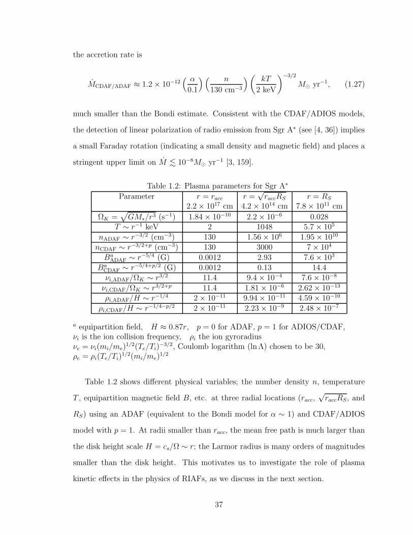
Table 1.2: Plasma parameters for Sgr A∗

Parameter r = racc r =√raccRS r = RS

2.2 × 1017 cm 4.2 × 1014 cm 7.8 × 1011 cm

ΩK =√

GM∗/r3 (s−1) 1.84 × 10−10 2.2 × 10−6 0.028T ∼ r−1 keV 2 1048 5.7 × 105

nADAF ∼ r−3/2 (cm−3) 130 1.56 × 106 1.95 × 1010

nCDAF ∼ r−3/2+p (cm−3) 130 3000 7 × 104

BaADAF ∼ r−5/4 (G) 0.0012 2.93 7.6 × 103

BaCDAF ∼ r−5/4+p/2 (G) 0.0012 0.13 14.4

νi,ADAF/ΩK ∼ r3/2 11.4 9.4 × 10−4 7.6 × 10−8

νi,CDAF/ΩK ∼ r3/2+p 11.4 1.81 × 10−6 2.62 × 10−13

ρi,ADAF/H ∼ r−1/4 2 × 10−11 9.94 × 10−11 4.59 × 10−10

ρi,CDAF/H ∼ r−1/4−p/2 2 × 10−11 2.23 × 10−9 2.48 × 10−7

a equipartition field, H ≈ 0.87r, p = 0 for ADAF, p = 1 for ADIOS/CDAF,νi is the ion collision frequency, ρi the ion gyroradiusνe = νi(mi/me)

1/2(Te/Ti)−3/2, Coulomb logarithm (lnΛ) chosen to be 30,

ρe = ρi(Te/Ti)1/2(mi/me)

1/2

Table 1.2 shows different physical variables; the number density n, temperature

T , equipartition magnetic field B, etc. at three radial locations (racc,√raccRS, and

RS) using an ADAF (equivalent to the Bondi model for α ∼ 1) and CDAF/ADIOS

model with p = 1. At radii smaller than racc, the mean free path is much larger than

the disk height scale H = cs/Ω ∼ r; the Larmor radius is many orders of magnitudes

smaller than the disk height. This motivates us to investigate the role of plasma

kinetic effects in the physics of RIAFs, as we discuss in the next section.

37

1.5 Motivation

As discussed in the previous section, there is ample evidence that RIAFs are colli-

sionless, with the Coulomb collision time much longer than accretion time (see Table

1.2). However, most studies of the MRI have used ideal MHD equations, which are

formally valid only for collisional, short mean free path plasmas. A collisionless anal-

ysis should use the Vlasov equation [104] which describes the time evolution of the

distribution function of a collisionless plasma in a 6-D phase space. In cases when

the scales of interest are much larger than the ion Larmor radius (e.g., in RIAFs ion

Larmor radius is ∼ 108 times smaller than the disk height scale, the scale of largest

eddies in MRI turbulence), one can average over the fast gyromotion to obtain the

drift kinetic equation (DKE) describing the distribution function in a 5-D phase space

[110, 180]. Collisionless plasmas are different from the collisional MHD plasmas, in

that the pressure is anisotropic with respect to the magnetic field, and rapid thermal

conduction can occur along the field lines.

Quataert and coworkers [158], used the DKE to study the collisionless MRI in the

linear regime. They found that with an equal vertical and azimuthal fields, the fastest

growing mode is twice as fast as in MHD and occurs at a much larger length scale.

The aim of the thesis is to follow up their work with numerical simulations of the

MRI in the kinetic regime. A method based on the DKE that evolves the distribution

function in a 5-D phase space is more expensive than the 3-D MHD simulations. A

less expensive approach (and equivalent to the DKE in the linear regime) is to use

the kinetic MHD (KMHD) equations with Landau fluid closure for parallel heat flux

[180]. We started by showing the equivalence of linear modes in the drift kinetic

and KMHD formalisms (the stable fast, Alfven, slow, and entropy modes, and the

unstable MRI) in a Keplerian disk [176]. This was followed up by nonlinear KMHD

simulations in a local shearing box [177].

Transition of the MRI from collisionless to collisional regime was studied linearly,

38

using a BGK collision operator [176]. Transition from kinetic to the Braginskii regime

occurs as the mean free path becomes short compared to the parallel wavelength,

λmfp ≪ λ‖ ≡ 2π/k‖; for the fastest growing mode this corresponds to ν . Ω√β,

where ν is the collision frequency. As collision frequency is increased further (ν & Ωβ),

anisotropic stress becomes negligible compared to the Maxwell stress, and transition

to MHD occurs. Differences between the kinetic and MHD regimes is striking at large

β’s. A crucial difference from MHD is the presence of damped modes, indicating

a possibility of wave-particle interactions in form of Landau and Barnes damping

[113, 18, 182]. Balbus and Islam [12, 96] have studied MRI in the weakly collisional

Braginskii regime and found agreement with our results.

The ZEUS MHD code [185, 186] is modified to include anisotropic pressure, and

parallel thermal conduction based on Landau fluid closure [180]. Nonlinear KMHD

simulations are done in a local shearing box limit [86]. The adiabatic invariant,

µ = p⊥/B, is conserved in collisionless plasmas, as a result, pressure anisotropy

(p⊥ > p‖) is created as magnetic field is amplified by the MRI. Pressure anisotropy

cannot become large (p⊥/p‖ − 1 . few/β⊥), as mirror and ion-cyclotron instabilities

will isotropize the pressure by pitch angle scattering. Subgrid models of pitch angle

scattering by these instabilities at the Larmor radius scale have been included. Pres-

sure anisotropy gives rise to a stress in addition to the usual Maxwell and Reynolds

stress in MHD [177]. Pressure anisotropy driven instabilities are expected to arise in

any collisionless plasma, when the field strength changes in a β & 1 plasma, e.g., the

solar wind [123, 98], magnetosphere [192, 66], and galaxy clusters [170].

The next step is to include collisionless effects in global MHD simulations [188].

Anisotropic thermal conduction is expected to change the convective stability cri-

terion from an outward increasing entropy to an outward increasing temperature

[10, 11, 148]. Self-similar solutions using saturated (isotropic) conduction have shown

significant differences from standard non-conducting ADAF models [130, 190]. While

39

implementing anisotropic thermal conduction in global MHD simulations we discov-

ered that the centered differencing of anisotropic thermal conduction can give rise to

heat flowing from lower to higher temperatures, causing the temperature to become

negative in regions with large temperature gradients, e.g., disk corona interface. We

have developed a new numerical method that uses slope limiters to ensure that the

temperature extrema are not amplified by anisotropic conduction [175]. Global nu-

merical simulations with anisotropic thermal conduction can tell us about the global

structure of RIAFs. These, combined with the insights on local energy dissipation in

disks from the local KMHD simulations, can shed light on their low luminosity.

1.6 Overview

The main body of the thesis (chapters 3, 4, and 5) is based on three papers, the

first on the transition of the MRI from collisionless to the collisional regime [176], the

second on the shearing box simulations of the collisionless MRI [177], and the third on

numerical implementation of anisotropic conduction in presence of large temperature

gradients [175].

Chapter 2 introduces the kinetic MHD formalism. We begin with the Vlasov

description of a collisionless plasma, and derive the drift kinetic equation (DKE) in

the limit of length scales much larger than the Larmor radius, and frequencies much

smaller than the gyrofrequency. Moments of the DKE with an anisotropic pressure

tensor are called the kinetic MHD (KMHD) equations. The KMHD equations are

closed by the ‘3+1’ Landau fluid closure for heat flux along the field lines. Landau

closure is equivalent to a Pade approximation to the drift kinetic linear response

function. We discuss different ways to implement the nonlocal closure in a numerical

simulation. We show that the moment equations with a BGK collision operator

recover the Braginskii equations in the high collisionality regime.

40

Chapter 3, which is based on [176], describes the transition of the MRI from

collisionless to the collisional regime. Linear modes of a magnetized, collisionless

plasma in a Keplerian rotation are derived using both the DKE and the KMHD

equations with Landau closure for the heat flux. The two methods agree very well

for the real and imaginary parts for the frequency response; this motivates kinetic

MHD simulations of the collisionless MRI. The presence of damped modes in the

collisionless regime can cause waves to be damped by Landau/Barnes damping at

large scales, instead of being damped only at small scales as in MHD with small

resistivity and viscosity. A BGK collision operator is used to study the transition of

the MRI from collisionless to the collisional (MHD) regime; the transition from kinetic

to the Braginskii regime occurs when the mean free path becomes small compared to

the wavelength, for the fastest growing mode this corresponds to ν & Ω√β.

Chapter 4 presents results from the nonlinear shearing box simulations of the colli-

sionless MRI. Pressure anisotropy (p⊥ > p‖) is created because of adiabatic invariance

(µ = p⊥/B), as magnetic field is amplified by the MRI. The effect of p⊥ > p‖ is to

make the field lines stiffer. If the pressure anisotropy is allowed to become arbitrarily

large, the stiff field lines (because of p⊥ > p‖) can result in the stabilization of all

the MRI modes into small amplitude anisotropic Alfven waves. However, at large

pressure anisotropies (p⊥/p‖ − 1 > (a few)/β), mirror and ion-cyclotron instabilities

are expected to arise. Although the mirror instability is present in the kinetic MHD

approximation, the resolution (and hence the growth rate) is not enough to keep

the pressure anisotropy within the marginal anisotropy. The ion-cyclotron instabil-

ity is ordered out of the drift kinetic ordering. Therefore, subgrid models for pitch

angle scattering due to these instabilities are included. Pitch angle scattering due

to microinstabilities imposes an MHD-like dynamics on collisionless plasmas, this is

the reason MHD provides a good approximation for many collisionless plasmas in

astrophysics, e.g., the solar wind, the magnetosphere, and the interstellar medium.

41

Modifications to the ZEUS MHD code, to include the kinetic MHD terms, are de-

scribed. The key result of the collisionless MRI simulations is that anisotropic stress,

a qualitatively new mechanism to transport angular momentum, is as important as

the dominant Maxwell stress in MHD. This can also affect the energetics; in partic-

ular the rate at which anisotropic pressure (collisionless damping is included in it)

heats ions and electrons can be comparable. If electron heating is comparable to ion

heating, it will be difficult to maintain Te ≪ Ti as required by some RIAF models.

Chapter 5 is the result of our attempts to carry out global non-radiative disk sim-

ulations. The aim was to include the effect of anisotropic conduction on global MHD

disk simulations [188]. The initial condition consists of a constant angular momentum

torus surrounded by a hot, low density corona. We were running into numerical diffi-

culties with this initial set up; the temperature was becoming negative at some grid

points near the disk corona interface. This motivated us to investigate the effect of

anisotropic conduction in regions of high temperature gradient. Chapter 5 describes

simple tests where centered differencing of anisotropic thermal conduction results in

heat flowing from lower to higher temperatures, resulting in negative temperature at

large temperature gradients. We introduce a new numerical method based on limit-

ing the transverse temperature gradient; this ensures that heat flows from higher to

lower temperatures and the temperature extrema are not amplified. Many tests and

convergence studies are described.

Chapter 6 concludes the thesis with an outline of possible future work. Future

work include global disk simulations with anisotropic thermal conduction, local simu-

lations with more sophisticated models for non-local anisotropic thermal conduction,

and more accurate drift kinetic simulations evolving the distribution function in a

5-D phase space.

Appendix A describes the efficiency of black hole accretion based on a simple

pseudo-Newtonian potential which captures key general relativistic effects [145]. Also

42

presented is the derivation of spherically symmetric, steady accretion.

Appendix B shows the derivation of closures for p‖ and p⊥, using the DKE with

a BGK collision operator, in both high and low collisionality limit. These have been

used in Chapter 2 to show the equivalence of the drift kinetic formalism and the

kinetic MHD approximation with Landau closure for heat flux.

Appendix C describes the modifications to the ZEUS MHD code to include the

kinetic MHD terms, anisotropic pressure and anisotropic thermal conduction based on

Landau fluid closure. This also includes some tests of the collisionless aspects of the

code, e.g., damping of a linear fast mode, mirror instability in an initially anisotropic

plasma (p⊥ > p⊥), shear generated pressure anisotropy and firehose instability driven

by the anisotropy (p‖ > p⊥).

Appendix D describes the error analysis of a time series where the sampling time

is smaller than the correlation time. For such a data, all entries are not independent

and the standard deviation is no a correct measure of uncertainty. This method based

on [144] is used to put error bars on the time and volume averaged quantities derived

from the shearing box simulations (in Chapter 4).

43

Chapter 2

Description of collisionless plasmas

Macroscopically collisionless plasmas, with collision mean free path comparable to the

system size, are ubiquitous in astrophysics, e.g., the solar wind, earth’s magnetotail,

radiatively inefficient accretion flows (RIAFs), and X-ray clusters. Fluid theories,

such as hydrodynamics and MHD, are applicable only when the mean free path is

much smaller than the system size, but are routinely used even when the plasma is

collisionless. While fluid theories are sometimes useful even outside of their rigorous

regime of validity, collisionless plasmas can be quite different from MHD plasmas. For

example, whereas, viscous and resistive dissipation at small scales are the only ways

to dissipate kinetic and magnetic energies into thermal motion in MHD, collisionless

damping at large scales is an important source of heating in collisionless plasmas.

Although kinetic instabilities may enforce an MHD-like behavior, collisionless effects

can be crucial, especially to understand energetics and particle acceleration.

In this chapter we discuss several descriptions of collisionless plasmas valid in dif-

ferent approximations. We start with the Vlasov equation, the most detailed descrip-

tion of a collisionless plasma, which describes the time evolution of the distribution

function in a 6-D phase space. The drift kinetic equation (DKE) is obtained from

the Vlasov equation, in the limit when length scales are much larger than the Larmor

44

radius and time scales much longer than the gyroperiod. Moments of the DKE result

in kinetic MHD (KMHD) equations, where pressure is anisotropic with respect to the

magnetic field direction. Landau fluid closure for heat flux along the field lines, which

recovers the correct kinetic response in the linear regime, is described.

2.1 The Vlasov equation

A complete statistical description of the species ‘s’ in a collisionless plasma involves

a distribution function Fs in a 6Ns dimensional phase space, where Ns is the total

number of particles of species ‘s’. The distribution function, Fs, satisfies the Liouville

equation for an N-body system [74],

DFs

Dt≡ ∂Fs

∂t+

Ns∑

i=1

vi ·∂Fs

∂xi

+Ns∑

i=1

ai ·∂Fs

∂vi

= 0, (2.1)

corresponding to the conservation of probability, where x, v, and a are position,

velocity, and acceleration respectively, and D/Dt is the Lagrangian derivative in the

6Ns dimensional phase space [104]. Reduced distributions are obtained by integrating

Fs over all but one, two, three, etc., particles.

Evolution for the single particle distribution function fs(x,v, t) is obtained by

integrating Eq. 2.1 over all but one particle’s phase space,

∂fs

∂t+ v · ∇fs +

[

qsms

(E + v × B) +Fg

ms

]

· ∇vfs = 0, (2.2)

where all terms of order the plasma parameter, g ≡ 1/nsλ3D ≪ 1 [135], are neglected.

The plasma parameter is the inverse of the number of particles in a Debye sphere.

The Debye length is the length scale over which plasma establishes quasineutrality,

λD =√

kTs/4πnsq2s , where ns, Ts are number density and temperature [104]. For an

ideal plasma, with effective shielding, nsλ3D ≫ 1 or g ≪ 1. The force of gravity is

45

denoted by Fg, and the electromagnetic fields are governed by the Maxwell equations

∇ · E = 4π∑

s

qs

∫

fsdv, (2.3)

∇ · B = 0, (2.4)

∂B

∂t= −c∇× E, (2.5)

∇×B = 4π∑

s

qsc

∫

fsvdv +1

c

∂E

∂t. (2.6)

The higher order terms (in g) that we neglect in the derivation of Eq. 2.2–negligible

compared to the collective force due to plasma–arise because of scattering due to mi-

croscopic fields of nearby particles. Eq. 2.2 is the Vlasov equation (also known as the

collisionless Boltzmann equation) that describes the distribution function fs(x,v, t),

the probability of finding a particle of species ‘s’ in an interval dxdv at (x,v) in

phase space at time t. The Vlasov-Maxwell equations are more complicated than the

fluid equations as they involve seven independent variables t,x,v rather than four in

MHD, t,x. A collision operator, that takes into account the microscopic fields due to

individual charges, can be added on the right side of Eq. 2.2 to obtain the Boltzmann

equation. Going from 6Ns to 6 variables in phase space simplifies the description

considerably for an ideal plasma with g ≪ 1. Further simplifications can be made as

we show in the following sections.

2.2 The drift kinetic equation

The Vlasov equation can be simplified further if the Larmor radius (ρs) is much

smaller than the spatial scales (ρs/L≪ 1), and the gyroperiod (2π/Ωs) much smaller

than the time scales (Ωs ≫ ω). An asymptotic expansion in ρs/L = (ms/qs)(cv/BL) ≪

1 can reduce the number of variables by two; the gyration phase is irrelevant, and the

perpendicular velocity is governed by the adiabatic invariant, µ = v2⊥/2B [48].

46

To the lowest order, all particles drift with an E × B velocity perpendicular to

the field lines, and a parallel motion along the field lines. The parallel electric field

is small, E‖ ∼ O(1/qs) ∼ O(ǫ), as charges streaming along the magnetic field lines

will short it out. Lowest order term in the expansion of fs, f0s, is independent of

the gyrophase. We avoid the messy details of the derivation [109, 110, 165, 107], and

simply state the kinetic equation for the zeroth-order distribution function given by

(we follow Kulsrud’s derivation [109, 110])

∂f0s

∂t+ (VE + v‖b) · ∇f0s +

(

−b · DVE

Dt− µb · ∇B +

1

ms

(qsE‖ + Fg‖)

)

∂f0s

∂v‖= 0,

(2.7)

where b = B/B is the unit vector in magnetic field direction, VE = c(E × B)/B2 is

the drift velocity independent of species, and D/Dt ≡ ∂/∂t + (VE + v‖b) · ∇ is the

comoving derivative in phase space. The Maxwell equations to the lowest order gives

the charge neutrality condition,

∑

s

∫

qsf0sdv = 0, (2.8)

∑

s

∫

qsf0svdv = 0. (2.9)

Some remarks on the drift kinetic equation (DKE) are in order. Eq. 2.7 can

be interpreted as the conservation of probability in a 5-D phase space (x, µ, v‖) with

characteristics, dx/dt = VE +v‖b, and dv‖/dt = −b · DVE

Dt−µb ·∇B+ 1

ms(qsE‖+Fg‖).

Only the E×B drift shows up in the perpendicular drift, other drifts–curvature, ∇B,

etc., ∝ 1/qs–are higher order in ǫ in the drift-kinetic ordering. The force along the

field lines consists of the fluid inertial force (−b · DVE

Dt), the magnetic mirror force

(−µb · ∇B), the parallel electric force (qsE‖), and the parallel gravitational force

(Fg‖). Although E‖ ≪ E⊥ and can be dropped in the Ohm’s law, it needs to be kept

in the parallel particle dynamics where it ensures quasineutrality. The condition that

47

determines E‖ will be given in Eq. 2.27. The DKE evolves the distribution function

in a 5-D phase space (x, µ, v‖), with µ a parameter. A term with ∂/∂µ does not

appear in Eq. 2.7 as dµ/dt = 0 along the characteristics.

2.3 Kinetic MHD equations

In the drift-kinetic approximation, particles free stream along the field lines, but

move with the field lines in the perpendicular direction. This fluid-like behavior in

the perpendicular plane restores the possibility of a fluid description of a ρs/L ≪ 1

plasma.

Moments of the Vlasov equation combined with the Maxwell equations in the

non-relativistic limit (ignoring the displacement current, ∂E/∂t, in Eq. 2.6) yields

the kinetic MHD equations [109, 110],

∂ρ

∂t+ ∇ · (ρV) = 0, (2.10)

ρ∂V

∂t+ ρ (V · ∇)V =

(∇× B) ×B

4π−∇ · P, (2.11)

∂B

∂t= ∇× (V × B) , (2.12)

P = p⊥I +(

p‖ − p⊥)

bb, (2.13)

p⊥ =∑

s

ms

∫

f0sv2⊥

2dv, (2.14)

p‖ =∑

s

ms

∫

f0s(v‖ −V · b)2dv, (2.15)

where V = VE + V‖b is the fluid velocity. Kinetic MHD, like MHD, is a single fluid

description of plasma obtained by combining the moments of all species. Kinetic

MHD appears similar to MHD, except the pressure is an anisotropic tensor unlike

an isotropic pressure in MHD; the pressure tensor is determined by moments of the

solution of the DKE, unlike the equation of state in MHD. The asymptotic ordering

48

in 1/qs leads to the ideal Ohm’s law [104]. In principle, equations for p‖ and p⊥ can be

derived from the moments of the DKE. However, because of the inherent complexity

of a phase space description, fluid approximations for closure are usually employed.

The simplest and the oldest approximation is the double adiabatic (CGL) approx-

imation, where heat flux is assumed to vanish [48],

d

dt

(

p⊥ρB

)

= 0, (2.16)

d

dt

(

p‖B2

ρ3

)

= 0. (2.17)

The assumption that the heat flux vanishes is valid only if the phase speed, ω/k‖,

is much larger than electron and ion thermal speeds, a cold plasma criterion almost

never satisfied for slow and fast magnetoacoustic waves at high β.1 Furthermore,

the CGL equations are non-dissipative, incapable of modeling collisionless damping.

The CGL closure is also known to give an incorrect marginal stability criterion for

the mirror instability, an instability that regulates pressure anisotropy in collisionless

plasmas [110, 180].

2.4 Landau fluid closure

In this section we describe a fluid closure that maintains the simplicity of the CGL

model, while including kinetic effects like Landau damping [180]. We also include

a simple BGK collision operator, which conserves number, momentum, and energy.

Fluid closures that incorporated kinetic effects like collisionless damping were first

derived in the electrostatic limit for nonlinear studies of drift-wave instabilities [79,

78, 54]. Snyder et al. [180] extended the closure to electromagnetic bi-Maxwellian

(anisotropic) plasmas; similar closures were obtained by [46]. Fluid closures that

1This cold plasma criterion is also not satisfied for Alfven waves, though the heat flux is zero forlinear Alfven waves in a uniform plasma.

49

capture kinetic effects are somewhat analogous to the flux limited diffusion methods

used in radiation transport [117, 131].

2.4.1 The moment hierarchy

Multiplying Eq. 2.7 by B, and using Eq. 2.12 leads to the kinetic equation in a

conservative form,

∂

∂tfsB+∇·[fsB(v‖b+VE)]+

∂

∂v‖

[

fsB

(

−b · DVE

Dt− µb · ∇B +

qsms

E‖

)]

= BC(fs),

(2.18)

where subscript ‘0’ has been suppressed. The term on the right is a BGK collision

operator [25]

C(fj) = −∑

k

νjk(fj − FMjk), (2.19)

where νj,k is the collision rate of species j with k. The collisions cause fj to relax to

a shifted Maxwellian with effective temperature of the species j and fluid velocity of

the species k,

FMjk =nj

(2πTj/mj)3/2exp

[

−−mj(v‖ − V‖k)2

2Tj− mjµB

Tj

]

, (2.20)

where Tj = (T‖j + 2T⊥j)/3.2

2A variant of this model is required to handle the large differences between energy and momentumrelaxation rates that can occur in some cases, but this simpler model is sufficient for the case athand, where V‖,e = V‖,i to lowest order.

50

We define the velocity moments as:

ns =

∫

fsdv, nsV‖s =

∫

fsv‖dv,

p‖s = m

∫

fs(v‖ − V‖)2dv, p⊥s = m

∫

fsµBdv,

q‖s = m

∫

fs(v‖ − V‖)3dv, q⊥s = m

∫

fsµB(v‖ − V‖)dv,

r‖,‖s = m

∫

fs(v‖ − V‖)4dv, r‖,⊥s = m

∫

fsµB(v‖ − V‖)2dv,

r⊥,⊥s = m

∫

fsµ2B2dv.

Specializing to the case of an electron-proton plasma, and using the charge neutrality

condition (Eqs. 2.8 and 2.9), n = ne = ni and V‖ = V‖e = V‖i. In this limit when

electrons and protons drift at equal velocity, the only role of collisions is to isotropize

51

the distribution function. Taking appropriate moments of Eq. 2.18,

∂n

∂t+ ∇·(nV) = 0, (2.21)

∂V‖∂t

+ V · ∇V‖ + b·(

∂VE

∂t+ V · ∇VE

)

+∇ · (bp‖s)nms

− p⊥s∇ · bnms

− qsE‖

ms

= 0, (2.22)

∂p‖s∂t

+ ∇ · (p‖sV) + ∇ · q‖s + 2p‖sb · ∇V · b − 2q⊥s∇ · b

= −2

3νs(p‖s − p⊥s), (2.23)

∂p⊥s

∂t+ ∇ · (p⊥sV) + ∇ · q⊥s + p⊥s∇ · V − p⊥sb · ∇V · b

+ q⊥s∇ · b = −1

3νs(p⊥s − p‖s), (2.24)

∂q‖s∂t

+ ∇·(Vq‖s) + ∇ · (br‖,‖s) + 3q‖sb · ∇V · b

− 3p‖snms

b · ∇p‖s + 3

(

p⊥sp‖snms

−p2‖s

nms− r‖,⊥s

)

∇ · b = −νsq‖s, (2.25)

∂q⊥s

∂t+ ∇·(Vq⊥s) + ∇ · (br‖,⊥s) + q⊥s∇·(V‖b) − p⊥s

nms

b · ∇p‖s

+

(

p2⊥s

nms

− p⊥sp‖snms

− r⊥,⊥s + r‖,⊥s

)

∇ · b = −νsq⊥s, (2.26)

where ρ = n(mi +me), V = VE +V‖b, νi = νii +νie and νe = νee +νei, and q‖s = bq‖s

and q⊥s = bq⊥s are thermal fluxes of p‖s and p⊥s along the field lines; perpendicular

heat flux vanishes as ρs/L ≪ 1. The perpendicular equation of motion is given by

the perpendicular component of Eq. 2.11, whose parallel component is equivalent to

Eq. 2.22. The condition V‖i = V‖e, and Eq. 2.22 gives [110],

E‖ =

∑

s(qs/ms)b · ∇ ·Ps∑

s(nsq2s/ms)

. (2.27)

Eqs. 2.21-2.24, like Eqs. 2.10-2.13, are not complete, and need a closure equation for

q‖s and q⊥s. In the next subsection we introduce Landau fluid closure for heat fluxes.

52

Conservation properties

The moment equations (Eqs. 2.10, 2.11, 2.23 and 2.24) conserve momentum and total

energy irrespective of the closure for higher moments. Combining Eqs. 2.10 and 2.11

gives the momentum conservation equation,

∂

∂t(ρV) = −∇·

[

ρVV +

(

B2

8πI− BB

4π

)

+ P

]

, (2.28)

where p‖ = p‖i + p‖e and p⊥ = p⊥i + p⊥e.

Total energy (the sum of kinetic, magnetic, and thermal energies), defined as

Γ = ρV 2/2 +B2/8π + p⊥ + p‖/2, is also conserved as

∂Γ

∂t= −∇·

[(

1

2ρV 2 + p⊥ +

1

2p‖

)

V

]

−∇·[

B × (V × B)

4π

]

−∇ · (V · P) −∇ · q,

(2.29)

where q = (q⊥ + q‖/2)b, and q‖ = q‖i + q‖e and q‖ = q‖i + q‖e.

2.4.2 The 3+1 Landau closure

A simple model which evolves p‖ and p⊥, and truncates the moment hierarchy with

Eqs. 2.23 and 2.24, using closure approximations for q‖ and q⊥ is called a “3+1

model,” as it evolves 3 parallel moments (n, u‖, p‖) and 1 perpendicular moment (p⊥)

[180].

The 3 + 1 closure is derived by writing q‖ and q⊥ in terms of the lower moments

and δB, and solving for coefficients by matching with the linear kinetic response.

This gives [180]

q‖s = −n√

8

πvt‖s

ik‖T‖s|k‖|

, (2.30)

q⊥s = −n√

2

πvt‖s

ik‖T⊥s

|k‖|+ n

√

2

πvt‖sT⊥s

(

1 − T⊥s

T‖s

)

ik‖δB

|k‖|B, (2.31)

53

where vt‖s =√

T‖s/ms, and k‖ is the parallel wavenumber of small perturbation. The

second term in the closure for q⊥s vanishes in the electrostatic limit or if pressure is

isotropic, and is needed to conserve µ linearly [180].

Substituting the closures, Eqs. 2.30 and 2.31, into Eqs. 2.21-2.24 yields the density

response

δns =in

k‖T‖sqsE‖R3(ζs) + n

δB

B

[

1 − T⊥s

T‖sR3(ζs)

]

, (2.32)

and the perpendicular pressure response

p⊥s = − ip⊥s

k‖T‖sqsE‖R3(ζs) + 2p⊥s

δB

B

[

1 − T⊥s

T‖s

(

R3(ζs2

+R1(ζs

2

)]

, (2.33)

where ζs = ω/√

2|k‖|vt‖s, and R3(ζs) is the three-pole Pade approximation of the

electrostatic response function

R3(ζs) =2 − i

√πζs

2 − 3i√πζs − 4ζ2

s + 2i√πζ3

s

, (2.34)

and R1(ζs) is a one-pole model of R(ζs), R1(ζs) = 1/(1 − i√πζs). The electrostatic

response function, R(ζs) = 1 + ζsZ(ζs), where Z(ζ) = (1/√π)∫

dt exp(−t2)/(t − ζ),

arises frequently in linearized moments of the Vlasov equation (or the DKE). The

3 + 1 model recovers the fully kinetic response function in both asymptotic limits,

ζs ≪ 1 and ζs ≫ 1, and provides a good approximation in the intermediate regime.

Figs. (1)-(4) in [180] show that Landau closure is a good approximation for the linear

response function from the DKE. While the linear response function in CGL (and

MHD) approximation shows no imaginary part in frequency, Landau closure gives

collisionless damping rates consistent with the DKE.

The complete 3 + 1 system of equations is given by Eqs. 2.10-2.13, and Eqs. 2.23

and 2.24, closed by the inverse Fourier transform of Eqs. 2.30 and 2.31. In Section

2.6 we discuss ways of computing the heat fluxes in coordinate space from the Fourier

54

space expressions.

2.5 Collisional effects

Collisions serve two roles, first they isotropize the pressure tensor, and second they

reduce the heat fluxes. With the BGK collision operator, a pitch angle scattering

term that isotropizes pressure appears in equations for p‖ and p⊥ (terms on the right

side of Eqs. 2.23 and 2.24). Certain collisional effects, such as perpendicular diffusion,

resistive effects, etc., are not included because of the drift kinetic ordering (Ωs ≫ ω,

ν); also not included is the collisional heat transfer from one species to another.

To extend Landau closure to the collisional regime, it is useful to write Eqs. 2.23

and 2.24 in a form similar to Braginskii’s equations [37]. This is done by defining an

average pressure, ps = (p‖s + 2p⊥s)/3, a differential pressure, δps = p‖s − p⊥s, and a

heat flux, qs = q‖s/2 + q⊥s. The pressure tensor, Ps, can be divided into an isotropic

part, psI, and an anisotropic stress, Πs = −δpsI/3 + δpsbb, with δps = (p‖s − p⊥s).

Combining Eqs. 2.23 and 2.24, then gives [180]

dps

dt+

5

3ps∇ ·V = −2

3∇ · (bqs) −

2

3Πs : ∇V, (2.35)

dδps

dt+

5

3δps∇ ·V + Πs : ∇V + 3psb · ∇V · b − ps∇ · V − 3q⊥∇ · V

+ ∇ · [b(q‖s − q⊥s)] = −νsδps. (2.36)

2.5.1 The high collisionality limit

In the high collisionality limit, ν ≫ ω, the above equations yield approximation

to the Braginskii transport equations in the ν ≪ Ωs regime, as required by the

initial ordering. An expansion in 1/νs of Eqs. 2.25, 2.26, and 2.36 implies that

55

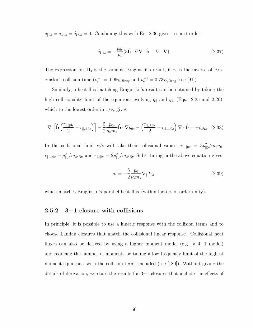
q‖0s = q⊥0s = δp0s = 0. Combining this with Eq. 2.36 gives, to next order,

δp1s = −p0s

νs(3b · ∇V · b−∇ · V). (2.37)

The expression for Πs is the same as Braginskii’s result, if νs is the inverse of Bra-

ginskii’s collision time (ν−1i = 0.96τi,Brag and ν−1

e = 0.73τe,Brag; see [91]).

Similarly, a heat flux matching Braginskii’s result can be obtained by taking the

high collisionality limit of the equations evolving q‖ and q⊥ (Eqs. 2.25 and 2.26),

which to the lowest order in 1/νs gives

∇·[

b(r‖,‖0s

2+ r‖,⊥0s

)]

− 5

2

p0s

n0msb · ∇p0s −

(r‖,⊥0s

2+ r⊥,⊥0s

)

∇ · b = −νsqs. (2.38)

In the collisional limit r0’s will take their collisional values, r‖,‖0s = 3p2‖0/msn0,

r‖,⊥0s = p2‖0/msn0, and r‖,‖0s = 2p2

‖0/msn0. Substituting in the above equation gives

qs = −5

2

p0

νsms∇‖T0s, (2.39)

which matches Braginskii’s parallel heat flux (within factors of order unity).

2.5.2 3+1 closure with collisions

In principle, it is possible to use a kinetic response with the collision terms and to

choose Landau closures that match the collisional linear response. Collisional heat

fluxes can also be derived by using a higher moment model (e.g., a 4+1 model)

and reducing the number of moments by taking a low frequency limit of the highest

moment equations, with the collision terms included (see [180]). Without giving the

details of derivation, we state the results for 3+1 closures that include the effects of

56

collisions,

q‖s = −8nv2t‖s

ik‖T‖s

(√

8π|k‖|vt‖s + (3π − 8)νs), (2.40)

q⊥s = −nv2

t‖sik‖T⊥s(√

π2|k‖|vt‖s + νs

)

+

(

1 − T⊥s

T‖s

)

nv2t‖sT⊥ik‖δB

B(√

π2|k‖|vt‖s + νs

) . (2.41)

These closures allow a smooth transition from collisionless regime where collisionless

damping is important, to the collisional regime with only viscous (collisional) damp-

ing. These closures give results similar to those derived from the DKE with a collision

operator (in the linear regime), as shown for the case of MRI in Chapter 3. Thus,

Landau models can be used to study collisionless and marginally collisional (ω ∼ ν)

regimes. However, accurate modeling of all the collisional effects, particularly those

involving momentum exchange between species, requires a Braginskii formalism in

highly collisional regime (ν ≫ ω) or extension of the BGK model to use a velocity

dependent collision frequency.

2.6 Nonlinear implementation of closure

Landau fluid closure for heat fluxes (Eqs. 2.30 and 2.31) involve terms containing

ik‖/|k‖|. Numerical implementation of these in k-space is straightforward for elec-

trostatic problems, as magnetic perturbations vanish and a simple Fourier transform

along the magnetic field direction is needed. However, in more general problems,

heat fluxes need to be calculated along the total (equilibrium+perturbation) mag-

netic field, and so k‖ involves Fourier transforms along the perturbed field lines.

Linear approximation of parallel heat flux, q‖ ∝ b0 · ∇δT‖ + δb · ∇T‖, has a contri-

bution due to perturbed field lines. In an incompressible, ideally conducting plasma,

temperature is constant along a field line (q‖ = 0), but temperature gradient along

57

the unperturbed field lines gives a nonzero result. Thus, the calculation of heat fluxes

along the perturbed field lines is non-trivial.

For fully nonlinear, electromagnetic calculations one can use a Lagrangian coor-

dinate system moving with the field lines, and coordinates aligned with the magnetic

field. Then the standard fast Fourier transform (FFT) algorithm along the coor-

dinate can be used to evaluate closures. While Lagrangian methods are useful for

fusion plasma simulations where magnetic field fluctuations are small, in most as-

trophysical cases fields are turbulent with B . δB, making a grid aligned with field

lines extremely difficult to implement. Alternatively, in an Eulerian grid, one needs

to map T‖ from the simulation grid to a field line following coordinate system, carry

out the FFT, and then remap the result back to the simulation grid. FFTs can be

avoided by working with the real space form of closures. This involves convolutions

in one direction [O(N4) operations for N grid points in each direction], rather than

the FFT algorithm [O(N3 lnN) operations]. For example, the real-space form of the

collisionless 3+1 closure for q‖s(z), Eq. 2.40, is the convolution

q‖s = −n(

2

π

)3/2

vt‖s

∫ ∞

0

dz′T‖s(z + z′) − T‖s(z − z′)

z′g(

z′

λmfp

), (2.42)

where g(z′/λmfp) = 1 for z′ small compared to the mean free path, but g falls off

rapidly for z′ large compared to the mean free path (see Eq. 51 of [180]). In a very

low collisionality plasma, exact evaluation of the heat flux requires integrating a very

long distance along a magnetic field line, but in practice the integral can be cut off

at a few correlation lengths. Truncating the integral at z′ = L essentially means

that Landau damping is applied to modes with k‖ > 1/L, while Landau damping is

ignored for large scale k‖ < 1/L modes. Choice of an appropriate L could be made

by convergence studies.

58

0 1 2 3 4 50

0.5

1

1.5

2

2.5

3

3.5

4

4.5

5

kL/|k

ll|

γ L/γ

kin

k⊥ /|kll|=4, β⊥ =10,

4π(pll−p⊥ )/B2=−1.25

0 0.5 1 1.5 20

0.2

0.4

0.6

0.8

1

1.2

1.4

1.6

kL/k

||

γ/Ω k

zV

Az/Ω=0.3, β

z=104, Bφ=B

z

Figure 2.1: The dependence of the kinetic MHD growth rate, for a mirror mode andan MRI mode, on the assumed kL Landau damping parameter in the heat fluxes. Theoptimal 3-pole approximation to the plasma Z function is recovered if kL/k‖ = 1. Theplot on the left shows that the growth rate of a mirror instability is fairly sensitiveto the assumed kL. On the other hand, the plot on the right shows that the growthrate of an MRI mode is not very sensitive to the assumed value of kL (for theseparameters). Note that kL = 0 corresponds to an isothermal limit and kL → ∞corresponds to a CGL limit where parallel heat fluxes are ignored. The existenceof anomalous pitch-angle scattering by velocity-space microinstabilities may furtherreduce the sensitivity of the nonlinear MRI results to the assumed kL parameter.

A crude closure for heat fluxes

A crude closure for parallel heat fluxes is obtained by using a local approximation

where |k‖| in the denominator of Eqs. 2.40 and 2.41 is replaced by a parameter kL,

i.e.,

q‖s = −8nv2t‖s

ik‖T‖s

(√

8πkLvt‖s + (3π − 8)νs), (2.43)

q⊥s = −nv2

t‖sik‖T⊥s(√

π2kLvt‖s + νs

) +

(

1 − T⊥s

T‖s

)

nv2t‖sT⊥ik‖δB

B(√

π2kLvt‖s + νs

) . (2.44)

These are readily calculable local expressions for parallel heat fluxes that recovers the

correct growth/damping rate for a mode with wavenumber kL. Modes with |k‖| > kL

(|k‖| < kL) have a faster (slower) heat conduction rate than collisionless Landau

59

damping, but the final impact on the growth or damping rate of a mode depends on

the type of mode (see Figure 2.1 for examples of mirror and MRI modes). Note that

heat fluxes in Eqs. 2.43 and 2.44 with a constant kL are diffusive, like Braginskii’s

heat fluxes. The shearing box simulations of the MRI in the collisionless regime use

these local expressions [177]; the nonlinear results are not very sensitive to the choice

of kL, but do show some dependence (as shown in Chapter 4). However, there may

be velocity-space microinstabilities that enhance the effective pitch-angle scattering

rate, which may make the nonlinear results less sensitive to assumptions about kL

than one might at first think.

To improve on this in future work, there are several possible approaches that

could be taken, such as a direct evaluation of the non-local heat flux expressions like

Eq. 2.42, along field lines to some maximum length L. Another would be to use

better Pade approximations to the k-space operator corresponding to the Landau-

damping operator. For example, in Eqs. 2.30 and 2.31 the heat flux is proportional

to ik‖/|k‖|, which at present we approximate as ik‖/kL and then Fourier transform

to real space to get the local operator (1/kL)∇‖. A next order Pade approximation

to ik‖/|k‖ would be of the form α0ik‖/(1 + β2k2‖). Fourier transforming this gives the

operator (1 − β2∇2‖)

−1α0∇‖ [51]. If a fast iterative Krylov or Multigrid solver could

be developed to invert the (1−β2∇2‖) operator (which would be non-trivial because it

is an anisotropic operator corresponding to diffusion only along field lines), then this

could be a faster way to approximate the non-local heat flux operator that would be

relatively good over a range of k‖ instead of only near k‖ = kL. This procedure could

be made more accurate by using higher order Pade approximations.

Another way to improve the calculation of the heat flux while retaining a local

approximation could be by keeping more fluid moments before introducing a closure

approximation, and modifying the closure approximations to correspond to hyper-

collisions that selectively damp fine scales in velocity space. This would reduce the

60

number of fluid moments needed. Keeping higher order fluid moments before closing

is related to a kinetic calculation that uses higher order Hermite polynomial basis

functions in velocity space [77, 179]. While this is possible in principle, the rate of

convergence as more terms are added and its computational cost relative to other

options have not been evaluated.

Finally, another way to improve the calculation would be to do a direct 5-D

calculation of the drift-kinetic equation. This would be computationally challenging,

but would be feasible for a range of problems. It would be similar to 5-D gyrokinetic

simulations recently developed in fusion energy research that have made significant

contributions to understanding drift-wave turbulence in fusion devices [53, 97, 40].

2.6.1 The effects of small-scale anisotropy-driven instabilities

The MRI acts as a dynamo that amplifies the magnetic field. Conservation of the

magnetic moment µ = v2⊥/(2B) means that as the magnetic field fluctuates, the per-

pendicular pressure p⊥ will change, creating pressure anisotropies. As we will discuss

in more detail in Chapter 4, if these pressure anisotropies exceed a certain threshold,

they can drive velocity space instabilities (the mirror, cyclotron, and firehose insta-

bilities) that have very fast growth rates at small scales. These instabilities can drive

gyro-radius scale fluctuations that break adiabatic invariance and cause scattering to

reduce the pressure anisotropy back to threshold.

To estimate the magnitude of this enhanced scattering rate, consider Eq. 2.36 in

an incompressible limit, ∇ · V = 0 (as might be expected at high β for low Mach

number MRI-driven flows):

dδps/dt+ (3ps + δps)b · ∇V · b + ∇ · [b(q‖,s − q⊥,s)] = −νδps.

Expanding the magnetic field evolution equation in the incompressible limit, ∂B/∂t =

61

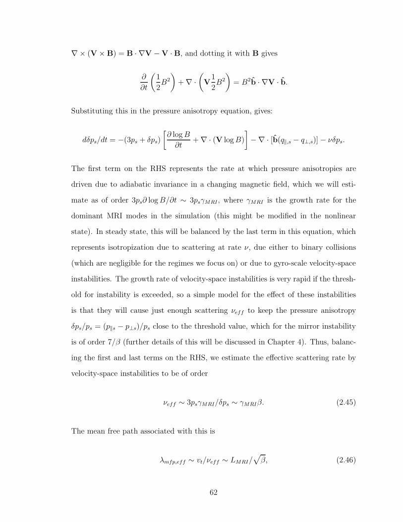
∇× (V × B) = B · ∇V − V · B, and dotting it with B gives

∂

∂t

(

1

2B2

)

+ ∇ ·(

V1

2B2

)

= B2b · ∇V · b.

Substituting this in the pressure anisotropy equation, gives:

dδps/dt = −(3ps + δps)

[

∂ logB

∂t+ ∇ · (V logB)

]

−∇ · [b(q‖,s − q⊥,s)] − νδps.

The first term on the RHS represents the rate at which pressure anisotropies are

driven due to adiabatic invariance in a changing magnetic field, which we will esti-

mate as of order 3ps∂ logB/∂t ∼ 3psγMRI , where γMRI is the growth rate for the

dominant MRI modes in the simulation (this might be modified in the nonlinear

state). In steady state, this will be balanced by the last term in this equation, which

represents isotropization due to scattering at rate ν, due either to binary collisions

(which are negligible for the regimes we focus on) or due to gyro-scale velocity-space

instabilities. The growth rate of velocity-space instabilities is very rapid if the thresh-

old for instability is exceeded, so a simple model for the effect of these instabilities

is that they will cause just enough scattering νeff to keep the pressure anisotropy

δps/ps = (p‖s − p⊥s)/ps close to the threshold value, which for the mirror instability

is of order 7/β (further details of this will be discussed in Chapter 4). Thus, balanc-

ing the first and last terms on the RHS, we estimate the effective scattering rate by

velocity-space instabilities to be of order

νeff ∼ 3psγMRI/δps ∼ γMRIβ. (2.45)

The mean free path associated with this is

λmfp,eff ∼ vt/νeff ∼ LMRI/√

β, (2.46)

62

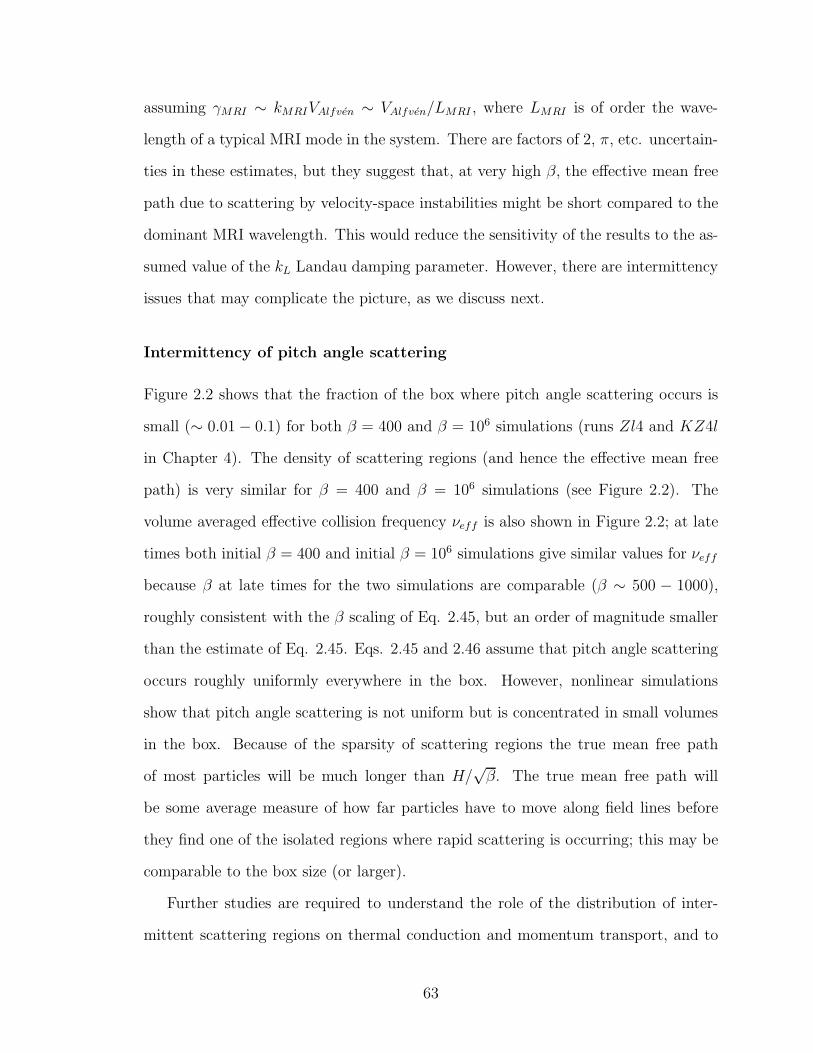
assuming γMRI ∼ kMRIVAlfven ∼ VAlfven/LMRI , where LMRI is of order the wave-

length of a typical MRI mode in the system. There are factors of 2, π, etc. uncertain-

ties in these estimates, but they suggest that, at very high β, the effective mean free

path due to scattering by velocity-space instabilities might be short compared to the

dominant MRI wavelength. This would reduce the sensitivity of the results to the as-

sumed value of the kL Landau damping parameter. However, there are intermittency

issues that may complicate the picture, as we discuss next.

Intermittency of pitch angle scattering

Figure 2.2 shows that the fraction of the box where pitch angle scattering occurs is

small (∼ 0.01 − 0.1) for both β = 400 and β = 106 simulations (runs Zl4 and KZ4l

in Chapter 4). The density of scattering regions (and hence the effective mean free

path) is very similar for β = 400 and β = 106 simulations (see Figure 2.2). The

volume averaged effective collision frequency νeff is also shown in Figure 2.2; at late

times both initial β = 400 and initial β = 106 simulations give similar values for νeff

because β at late times for the two simulations are comparable (β ∼ 500 − 1000),

roughly consistent with the β scaling of Eq. 2.45, but an order of magnitude smaller

than the estimate of Eq. 2.45. Eqs. 2.45 and 2.46 assume that pitch angle scattering

occurs roughly uniformly everywhere in the box. However, nonlinear simulations

show that pitch angle scattering is not uniform but is concentrated in small volumes

in the box. Because of the sparsity of scattering regions the true mean free path

of most particles will be much longer than H/√β. The true mean free path will

be some average measure of how far particles have to move along field lines before

they find one of the isolated regions where rapid scattering is occurring; this may be

comparable to the box size (or larger).

Further studies are required to understand the role of the distribution of inter-

mittent scattering regions on thermal conduction and momentum transport, and to

63

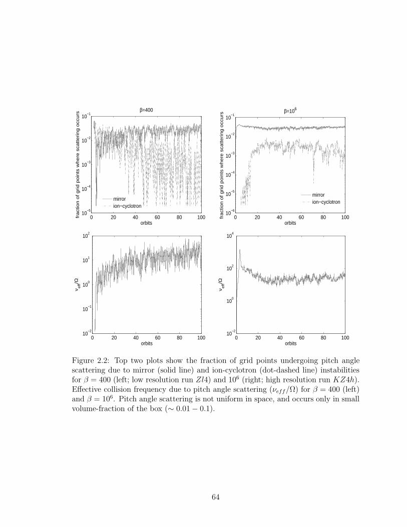
0 20 40 60 80 10010

−5

10−4

10−3

10−2

10−1

orbits

fra

ctio

n o

f g

rid

po

ints

wh

ere

sca

tte

rin

g o

ccu

rs

β=400

mirrorion−cyclotron

0 20 40 60 80 10010

−6

10−5

10−4

10−3

10−2

10−1

orbitsfr

act

ion

of

grid

po

ints

wh

ere

sca

tte

rin

g o

ccu

rs

β=106

mirrorion−cyclotron

0 20 40 60 80 10010

−2

10−1

100

101

102

orbits

ν eff/Ω

0 20 40 60 80 10010

−2

100

102

104

orbits

ν eff/Ω

Figure 2.2: Top two plots show the fraction of grid points undergoing pitch anglescattering due to mirror (solid line) and ion-cyclotron (dot-dashed line) instabilitiesfor β = 400 (left; low resolution run Zl4) and 106 (right; high resolution run KZ4h).Effective collision frequency due to pitch angle scattering (νeff/Ω) for β = 400 (left)and β = 106. Pitch angle scattering is not uniform in space, and occurs only in smallvolume-fraction of the box (∼ 0.01 − 0.1).

64

what extent does pitch angle scattering lead to MHD-like dynamics.

As we will find in Chapter 4, the limits on anisotropy provided by these velocity-

space instabilities cause the nonlinear kinetic MHD simulations of the MRI to be

qualitatively closer to regular MHD simulations of the MRI. However, even with these

limits on anisotropy, the anisotropic pressure component of the angular momentum

transport is found to be competitive with the usual Maxwell and Reynolds stress

transport mechanisms. The enhanced scattering by these velocity-space instabilities

may alter the relative electron/ion heating in MRI turbulence, a topic we leave for

future research.

The enhanced scattering by velocity-space instabilities can also cause an increase

in the effective Reynolds number (and thus a reduction of the effective magnetic

Prandtl number, the ratio of viscosity and resistivity) of high β MHD turbulence in

general. The possible implications of this are beyond the focus of this thesis, but they

have been discussed in a recent paper [170], on which I was a co-author.

To summarize, in this chapter we began with the most detailed Vlasov descrip-

tion of collisionless plasmas, and motivated the drift kinetic equation (DKE) in the

kρs ≫ 1, ω ≪ Ωs regime. Further simplification was introduced in the form of fluid

closures for parallel heat fluxes that reproduce correct kinetic behavior, and capture

collisionless damping. Fourier space representation of the heat fluxes, and the nonlo-

cal integral expression in coordinate space (and the ways to numerically compute it)

were indicated. A generalization to include the collisional effects, which reduces to

Braginskii’s result in ν ≫ ω regime, was given. A crude, local approximation for the

heat fluxes was presented, in which the parameter kL represents a typical wavenumber

of the mode. Only the local approximation has been used in the local shearing box

simulations of the collisionless MRI, leaving sophisticated treatments for the future.

Pitch-angle scattering by velocity space instabilities might provide a reduction of the

effective mean-free-path, which may contribute to reducing the sensitivity of the re-

65

sults to the assumed kL, but the scattering is found to be very intermittent spatially,

so the reduction in the mean free path might be less than one might expect at first.

66

Chapter 3

Transition from collisionless to

collisional MRI

This chapter is based on our paper on the transition of the MRI from the collisionless

to the collisional regime [176]. Calculations by Quataert and coworkers [158] found

that the growth rates of the magnetorotational instability (MRI) in a collisionless

plasma can differ significantly from those calculated using MHD, particularly at long

wavelengths. This can be important in hot accretion flows around compact objects

(see Section 1.4 for a review). In this chapter we study the transition from the colli-

sionless kinetic regime to the collisional MHD regime, mapping out the dependence

of the MRI growth rate on collisionality. The Landau fluid closure for parallel heat

flux, which recovers kinetic effects like Landau/Barnes damping, is used and the effect

of collisions is included via a BGK operator. The kinetic MHD equation of motion

has three forces: the isotropic pressure force, the magnetic force, and the anisotropic

pressure force. For β & 1 the transition from collisionless to Braginskii regime oc-

curs as the anisotropic pressure becomes small compared to the isotropic pressure

(ν & Ω√β); and the transition from Braginskii to MHD occurs when anisotropic

pressure force becomes negligible compared to the magnetic force (ν & Ωβ). In the

67

weak magnetic field regime where the Alfven and MRI frequencies ω are small com-

pared to the sound wave frequency k‖c0, the dynamics are still effectively collisionless

even if ω ≪ ν, so long as the collision frequency ν . k‖c0 (i.e., so long as the mean free

path is long compared to a wavelength); for an accretion flow this requires ν . Ω√β.

The low collisionality regime not only modifies the MRI growth rate, but also in-

troduces collisionless Landau or Barnes damping of long wavelength modes, which

may be important for heating of electrons and protons. The fastest growth rate in

the collisionless regime is ≈ twice faster than in MHD; moreover, the fastest growing

mode occurs at large length scales compared to the fastest growing MHD mode.

3.1 Introduction

Balbus and Hawley [14] showed that the magnetorotational instability (MRI), a local

instability of differentially rotating magnetized plasmas, is the most efficient source

of angular momentum transport in many astrophysical accretion flows (see Section

1.3 for a review). The MRI may also be important for dynamo generation of galactic

and stellar magnetic fields. Most studies of the MRI have employed standard MHD

equations which are appropriate for collisional, short mean free path plasmas, but it is

not obvious that this instability is relevant for collisionless, low luminosity accretion

flows (see Section 1.4; Table 1.2 shows the collsion frequency is small compared to the

rotation frequency). Quataert and coworkers ([158]; hereafter QDH) studied the MRI

in the collisionless regime using the kinetic results of Snyder, Hammett & Dorland

[180]. They showed that the MRI persists as a robust instability in a collisionless

plasma, but that at high β ≫ 1 (ratio of plasma pressure to magnetic pressure),

the physics of the instability is quite different and the kinetic growth rates can differ

significantly from the MHD growth rates.

One motivation for studying the MRI in the collisionless regime is to understand

68

radiatively inefficient accretion flows onto compact objects. An example of non-

radiative accretion is the radio and x-ray source Sagittarius A∗, which is powered by

gas accreting onto a supermassive black hole at the center of our galaxy (see Subsec-

tion 1.4.2 for a review). In radiatively inefficient accretion flow models, the accreting

gas is a hot, low density, plasma, with the proton temperature large compared to the

electron temperature (Tp ≈ 1012 K ≫ Te ≈ 1010 − 1012 K). In order to maintain such

a two-temperature configuration, the accretion flow must be collisionless in the sense

that the timescale for electrons and protons to exchange energy by Coulomb collisions

is longer than the inflow time of the gas (for models of Sagittarius A*, the collision

time close to the black hole is ≈ 7 orders of magnitude longer than the inflow time,

see Table 1.2).

In this chapter we extend the kinetic results of QDH to include collisions; we

study the behavior of the MRI in the transition from the collisionless regime to the

collisional MHD regime. Instead of using a more accurate (but very complicated)

Landau or Balescu-Lenard collision operator, we use the simpler Bhatnagar-Gross-

Krook (BGK) collision operator [25] that conserves number, momentum and energy.

There are several reasons for studying the MRI with a varying collision frequency:

(1) to gain additional understanding of the qualitatively different physics in the MHD

and kinetic regimes, (2) the key difference between the kinetic and MHD regimes

is that the pressure is anisotropic (with respect to the local magnetic field) in a

collisionless plasma (see Section 2.3). Even if particle collisions are negligible, high

frequency waves with frequencies ∼ the proton cyclotron frequency can isotropize the

proton distribution function (see Subsection 4.2.2). Our treatment of “collisions” can

qualitatively describe this process as well; and (3) the transition from the collisional to

the kinetic MRI could be dynamically interesting if accretion disks undergo transitions

from thin disks to hot radiatively inefficient flows (as has been proposed to explain,

e.g., state changes in X-ray binaries; [55]). There can be associated changes in the rate

69

of angular momentum transport (α), as disk transitions from collisional to collisionless

state, and vice versa.

We begin with the linearized drift kinetic equation with a BGK collision operator

and derive the exact closures for δp‖ and δp⊥; these are used to close the linearized ki-

netic MHD equations. We use Landau fluid closure for parallel heat fluxes, and show

that they are equivalent to the kinetic closures in both low and high collisionality

regimes; Landau fluids are considered because they are easier to implement compu-

tationally and we use them for local, nonlinear MHD disk simulations described in

Chapter 4. The kinetic MHD linear analysis shows the presence of damped modes at

all scales (see Figure 3.4), a feature absent in MHD.

3.2 Linearized kinetic MHD equations

The analysis is restricted to fluctuations that have wavelengths much larger than

proton Larmor radius and frequencies well below the proton cyclotron frequency. In

this limit, a plasma can be described by the following kinetic MHD equations (see

Section 2.3):

∂ρ

∂t+ ∇ · (ρV) = 0, (3.1)

ρ∂V

∂t+ ρ (V · ∇)V =

(∇× B) ×B

4π−∇ · P + Fg, (3.2)

∂B

∂t= ∇× (V × B) , (3.3)

P = p⊥I +(

p‖ − p⊥)

bb, (3.4)

where ρ is the mass density, V is the fluid velocity, B is the magnetic field, Fg is the

gravitational force, b = B/|B| is a unit vector in the direction of the magnetic field,

and I is the unit tensor. In equation (3.3) an ideal Ohm’s law is used, neglecting effects

such as resistivity. P is the pressure tensor that has different perpendicular (p⊥)

70

and parallel (p‖) components with respect to the background magnetic field (unlike

in MHD, where there is only a scalar pressure). The pressures are determined by

solving the drift kinetic equation given below. P should in general be a sum over all

species but in the limit where ion dynamics dominate and electrons just provide a

neutralizing background, the pressure can be interpreted as the ion pressure. This is

the case for hot accretion flows where Tp ≫ Te.

We assume that the background (unperturbed) plasma is described by a non-

relativistic Maxwellian distribution function with equal parallel and perpendicular

pressures (temperatures). Although the equilibrium pressure is assumed to be isotropic,

the perturbed pressure is not. We take the plasma to be differentially rotating,

but otherwise uniform (we neglect temperature and density gradients). Equilib-

rium state for equation (3.2) in presence of a subthermal magnetic field with ver-

tical (Bz = B0 sin θ) and azimuthal (Bφ = B0 cos θ) components gives a Keplerian

rotation (Ω ∝ R−3/2) profile.

In a differentially rotating plasma, a finite BR is sheared to produce a time-

dependent Bφ, which complicates the kinetic analysis (unlike in MHD, where a time-

dependent Bφ does not couple to axisymmetric disturbances; [14]); we therefore set

BR = 0. For linearization we consider fluctuations of the form exp[−iωt + ik · x],

with k = kRR + kzz, i.e., axisymmetric modes; we also restrict our analysis to local

perturbations for which |k|R≫ 1. Writing ρ = ρ0 + δρ, B = B0 + δB, p⊥ = p0 + δp⊥,

and p‖ = p0 + δp‖, V = φΩR + δV (with Keplerian rotation Ω(R)), and working in

cylindrical coordinates, the linearized versions of equations (3.1)-(3.3) become (see

71

QDH)

ωδρ = ρ0k · δV, (3.5)

−iωρ0δVR − ρ02ΩδVφ = −ikR

4π(BzδBz +BφδBφ) +

ikzBzδBR

4π− ikRδp⊥,(3.6)

−iωρ0δVφ + ρ0δVRκ2

2Ω=ikzBzδBφ

4π− ikz sin θ cos θ[δp‖ − δp⊥], (3.7)

−iωρ0δVz = −ikzBφδBφ

4π− ikz[sin

2 θδp‖ + cos2 θδp⊥], (3.8)

ωδBR = −kzBzδVR, (3.9)

ωδBφ = −kzBzδVφ − ikzBz

ω

dΩ

d lnRδVR +Bφk · δV, (3.10)

ωδBz = kRBzδVR, (3.11)

where κ2 = 4Ω2 + dΩ2/d lnR is the epicyclic frequency. To complete this system

of equations and derive the dispersion relation for linear perturbations, we need ex-

pressions for δp⊥ and δp‖ in terms of lower moments. These can be obtained by

taking moments of the linearized and Fourier transformed drift-kinetic equation that

includes a linearized BGK collision operator (see Section 2.2).

The drift-kinetic equation for the distribution function f , including the effects of

gravity is (see Section 2.2 for details)

∂f

∂t+(

v‖b + VE

)

· ∇f +

(

−b · DVE

Dt− µb · ∇B +

e

m(E‖ + Fg‖/e)

)

∂f

∂v‖= C (f) ,

(3.12)

where VE = c (E ×B) /B2, µ = (v⊥ −VE)2/2B is the magnetic moment (conserved

in our approximations in the absence of collisions), Fg‖ = GM∗mpR · b/R2, and

D/Dt = ∂/∂t +(

v‖b + VE

)

· ∇. The fluid velocity V = VE + bV‖, where the

E × B drift VE is determined by the perpendicular component of equation (3.2).

The parallel component of the gravitational force, Fg‖, is included as it is of the

same order as the parallel electric force. Notice the addition of a collision operator

on the right hand side to allow for generalization to collisional regimes. In the next

72

section we derive the linearly-exact kinetic expressions for δp‖ and δp⊥ using the BGK

collision operator in equation (3.12). We then compare these with Landau closure

approximations from Snyder et al. [180].

3.3 Kinetic closure including collisions

In this section we use a simple BGK collision operator [25] to calculate δp‖ and δp⊥

from equation (3.12). Since we consider only ion-ion collisions (see Subsection 2.4.1 for

multiple species), the BGK operator is CK (f) = −ν (f − FM) where ν is the ion-ion

collision frequency and FM is a shifted Maxwellian with the same density, momentum,

and energy as f (so that collisions conserve number, momentum, and energy). The

integro-algebraic BGK operator greatly simplifies the calculations while adequately

modeling many of the key properties of the full integro-differential collision operator.

In some situations, the effects of weak collisions can be enhanced in a more complete

collision operator due to sharp velocity gradients in the distribution function; we

ignore such effects in the present analysis.

In this section, we calculate the linearization of the drift-kinetic equation around

an accretion disk equilibrium, including equilibrium flows and gravity. A number of

complicated intermediate terms end up canceling, and the final forms of the closures

used (from equations (3.26-3.27) onwards) are identical to what one would get from

perturbing around a slab equilibrium with no flows. We carried out the more detailed

calculation to verify that there were no missing terms in the final closures.

The equilibrium distribution function f0 is given by

f0 =n0

(2πT0/m)3/2exp

(

− m

2T0

|v − V0|2)

, (3.13)

where V0 = VE0 + V‖0b0 is the Keplerian rotation velocity in the φ direction. Since

73

|v −V0|2 = (v‖ − V‖0)2 + 2µB0, f0 can be expressed in terms of

(

µ, v‖)

as

f0 =n0

(2πT0/m)3/2exp

(

− m

2T0

(

(v‖ − V‖0)2 + 2µB0

)

)

. (3.14)

We shall linearize the drift-kinetic equation and the BGK collision operator. The

distribution function is given as f = f0 + δf where δf is the perturbation in the

distribution function. The shifted Maxwellian that appears in the BGK collision

operator is given by

FM =NM

(2πTM/m)3/2exp

− m

2TM

(

(

v‖ − V‖M)2

+ 2µB)

. (3.15)

FM has three free parameters (NM , V‖M , TM) which are to be chosen so as to conserve

number, parallel momentum, and energy. When taking moments of the BGK opera-

tor, it is important to note that∫

d3v =∫

2π (B0 + δB) dµdv‖. From equation (3.15)

and conservation of number, momentum, and energy it follows that

NM = n0 + δn ≈ n0

(

1 +δB

B0

)

+ 2πB0

∫

dµdv‖δf, (3.16)

NMV‖M = NM(V‖0 + δV ) ≈ n0V‖0

(

1 +δB

B0

)

+ 2πB0

∫

dµdv‖δfv‖, (3.17)

NMTM = p0 + δp = p0 + (δp‖ + 2δp⊥)/3, (3.18)

δp‖ ≈ p0δB/B0 + 2πB0

∫

dµdv‖δfm(v‖ − V‖0)2, (3.19)

δp⊥ ≈ 2p0δB/B0 + 2πB0

∫

dµdv‖δfµmB0, (3.20)

where the approximate expressions retain only linear terms in perturbed quantities.

Linearizing the expression for the relaxed Maxwellian in equation (3.15) about f0,

74

the drift-kinetic BGK collision operator is given by

CK (δf) = −νδf + νf0 ×(

δn

n0− 3δT

2T0

)

+m

T0

(

(

v‖ − V‖0)

δu+(

v‖ − V‖0)2 δT

2T0

)

− mµB0

T0

(

δB

B0

− δT

T0

)

.(3.21)

The drift-kinetic equation including the BGK operator can be linearized to obtain

the following equation for δf

δf = Vφ0(v‖ − V‖0)f0 sin θ(δBφ sin θ − δBz cos θ)m

T0B0+

m(

v‖ − V‖0)

f0

T0

(

−iω + ik‖(

v‖ − V‖0)

+ ν) ×

(

−ik‖µδB +

(

eE‖ + Fg‖

)

m

)

+νf0

(

−iω + ik‖(

v‖ − V‖0)

+ ν) ×

(

δn

n0

− 3

2

δT

T0

+m(v‖ − V‖0)δu

T0

+m(v‖ − V‖0)

2

2T0

δT

T0

+mµB0

T0

δT

T0

− mµδB

T0

)

,(3.22)

where Fg‖ = GM∗mpδBR/B0R2 is the component of gravitational force in the di-

rection of magnetic field. Choosing a compact notation where −iω sin θ(δBφ sin θ −

δBz cos θ)mVφ0/eB0 +Fg‖/e + E‖ → E‖, the moments of the perturbed distribution

function δf in drift coordinates (v‖, µ),∫ (

1, 2µB0, (v‖ − V‖0)2)

δf2πB0dµdv‖ give

δn

n0

=δB

B0

(1 −R) +eE‖

ik‖T0

R− ζ2

(

δn

n0

− 3

2

δT

T0

)

Z +

(

δT

T0

− δB

B0

)

Z

+√

2δV

c0R +

(

δT

T0+ 2i sin θ

k‖Vφ0

ν

(δBφ sin θ − δBz cos θ)

B0

)

ζR

, (3.23)

δp⊥p0

= 2δB

B0(1 −R) +

eE‖

ik‖T0R− ζ2

(

δn

n0− 3

2

δT

T0

)

Z + 2

(

δT

T0− δB

B0

)

Z

+√

2δV

c0R +

(

δT

T0+ 2i sin θ

k‖Vφ0

ν

(δBφ sin θ − δBz cos θ)

B0

)

ζR

, (3.24)

δp‖p0

= −2δB

B0

ζ2R +eE‖

ik‖T0

(

1 + 2ζ2R)

− ζ2

2

(

δn

n0

− 3

2

δT

T0

)

ζR

+ 2

(

δT

T0

− δB

B0

)

ζR+√

2δV

c0

(

1 + 2ζ2R)

+

(

δT

T0+ 2i sin θ

k‖Vφ0

ν

(δBφ sin θ − δBz cos θ)

B0

)

ζ(

1 + 2ζ2R)

. (3.25)

75

The parallel electric field, E‖, can be eliminated by taking appropriate combinations

of these three equations, giving

δρ

ρ0− δp⊥

p0= −δB

B0(1 − R) + ζ2Z

(

δT

T0− δB

B0

)

, (3.26)

and

(

1 + 2ζ2R) δρ

ρ0

− Rδp‖p0

=δB

B0

(

1 + 2ζ2R− R)

− ζ2 (Z − 2ζR)

(

δρ

ρ0

− δT

2T0

− δB

B0

)

,

(3.27)

where δT =(

2δT⊥ + δT‖)

/3, δB = b0 ·δB, ζ = (ω + iν) /√

2|k‖|c0, ζ2 = iν/√

2|k‖|c0,

k‖ = b0 · k, T‖,⊥ = mp‖,⊥/ρ, and c0 =√

T0/m is the isothermal sound speed of the

ions. In equations (3.26) and (3.27), R = 1 + ζZ is the plasma response function,

where

Z (ζ) =1√π

∫

dxexp[−x2]

x− ζ(3.28)

is the plasma dispersion function [91]. Equations (3.26) and (3.27) can be substituted

into the linearized fluid equations 3.5-3.11 to derive the dispersion relation for the

plasma. The full closures are, however, very complicated, so it is useful to consider

several simplifying limits that isolate much of the relevant physics. In addition,

the solution of linearized kinetic MHD equations fully kinetic closures will give an

implicit equation for the growth rate (involving the Z function) that has to be solved

numerically.

The closure equations can be simplified in two limits, |ζ | ≪ 1, the collisionless

limit, and |ζ | ≫ 1, the high collisionality limit. The derivation of the asymptotic

solution for the closure equations in these two limits is given in Appendix B. In the

high collisionality limit,

δp⊥p0

=5

3

δρ

ρ0+ζ1ζ2

(

4

3+

5

9ζ21

)

δρ

ρ0− 2

ζ1ζ2

δB

B0, (3.29)

76

and

δp‖p0

=5

3

δρ

ρ0+ζ1ζ2

(

−2

3+

5

9ζ21

)

δρ

ρ0+ζ1ζ2

δB

B0, (3.30)

where ζ1 = ω/√

2|k‖|c0. Notice that in the limit that the collision frequency is very

high, ζ2 → ∞, one recovers the MHD result that the perturbations are adiabatic and

isotropic: δp‖/p0 = δp⊥/p0 = 5δρ/3ρ0.

For low collisionality, |ζ | ≪ 1, to second order in ζ ,

δp⊥p0

=δρ

ρ0

− i√πζ1

δB

B0

− πζ1ζ23

δρ

ρ0

+ ζ1ζ2

(

2 − π

3

) δB

B0

, (3.31)

and

δp‖p0

=δρ

ρ0− i

√πζ1

(

δρ

ρ0− δB

B0

)

+δρ

ρ0

(

4ζ1ζ2 − πζ21 − 7πζ1ζ2

6

)

+

δB

B0

(√πζ1ζ2 −

πζ1ζ26

− 2ζ2 − 4ζ2ζ

)

. (3.32)

To first order, there is no effect of collisions on the growth rate of the MRI; the

results above are then exactly same as equations (20) and (21) in QDH (who neglected

collisions entirely). Collisional effects modify the closure only at order ζ2, though one

has to go to this order to find the first order dependence of ω on ν in the dispersion

relation.

3.4 Comparison with Landau fluid closure

The results from last section provide expressions for δp⊥ and δp‖ in both low and high

collisionality regimes, |ζ | ≪ 1 and |ζ | ≫ 1, but it would be convenient to have a single

set of equations that can provide a robust transition between these two regimes. The

Landau fluid closure [180], which we discuss in Section 2.4, can do this.

The second order moments of the drift kinetic equation (Eq. 3.12) yield evolution

77

equations for δp⊥ and δp‖ (see, e.g., Eqs. 2.23 and 2.24). The linearized versions of

these equations, including a BGK collision operator, are given by 1

−iωδp‖ + p0ik · δv + ik‖q‖ + 2p0ik‖δv‖ − 3p0Ω cos θδBR

B0= −2

3ν(

δp‖ − δp⊥)

, (3.33)

and

−iωδp⊥ +2p0ik · δv+ ik‖q⊥−p0ik‖δv‖ +3

2p0Ω cos θ

δBR

B0

= −1

3ν(

δp⊥ − δp‖)

. (3.34)

As is usual with moment hierarchies, the above equations for δp‖,⊥ depend on third

moments of the distribution function, q‖ and q⊥, the parallel and perpendicular heat

fluxes.2 Snyder et al. [180] introduced closure approximations for q‖ and q⊥ that de-

termine δp⊥ and δp‖ without solving the full kinetic equation of the previous section

(see Section 2.4 for a review). These Landau-fluid approximations “close” equa-

tions (3.1)-(3.4) and allow one to solve for the linear response of the plasma.

The linearized heat fluxes of parallel and perpendicular pressures are given by

q⊥ = −p0c20

ik‖ (δp⊥/p0 − δρ/ρ0)(

√

π/2|k‖|c0 + ν) (3.35)

and

q‖ = −8p0c20

ik‖(

δp‖/p0 − δρ/ρ0

)

(√8π|k‖|c0 + (3π − 8) ν

) . (3.36)

As discussed in earlier work [180, 78, 77, 179], Landau-fluid closure approximations

provide n-pole Pade approximations to the exact plasma dispersion function Z(ζ) that

appears in the kinetic plasma response (see Section 2.4). These Pade approximations

1A comparison of our equations (3.33) and (3.34) with equations (30) and (31) in Snyder et al.(linearized version of Eqs. 2.23 and 2.24) shows that our equations have an extra term proportionalto the Keplerian rotation frequency; this is because [180] did not include gravitational effects andKeplerian rotation in their linearized equations.

2It is important to note that q‖ and q⊥ are the fluxes of p‖ and p⊥ along the field lines; thermalconduction perpendicular to field lines vanishes as the Larmor radius is tiny.

78

are thus able to provide robust results that capture kinetic effects such as Landau

damping, and that can also smoothly transition between the high and low ζ regimes.3

We have found, not surprisingly, that the fluid approximations remain robust when

collisions are included. That is, in all of the numerical tests we have carried out, we

have found good agreement between the results from equations (3.33)-(3.36) and the

asymptotic kinetic results from the previous section for the low and high collision-

ality regimes. All plots in this chapter are calculated with the Landau-fluid closure

equations (3.33)-(3.36).

The Landau-Fluid closure approximations provide a useful way to extend existing

non-linear MHD codes to study key kinetic effects (see Chapter 4). The closure ap-

proximations are independent of the frequency (or the Z function), so are straightfor-

ward to implement in a nonlinear initial value code (though, as discussed in Chapter 2

they do require FFT’s or non-local heat flux integrals to evaluate some terms[180, 78];

however, in nonlinear simulations discussed in Chapter 4 we use a simple local form

for heat flux). But one should remember that they are approximations and so do not

accurately model all kinetic effects in all regimes, particularly near marginal stabil-

ity ([126, 179, 52]), though it is generally found that they work fairly well in strong

turbulence regimes ([77, 147, 179, 52]).

As an aside, we note that the double adiabatic (CGL) closure [48], which is a

simpler closure approximation that sets q‖ = q⊥ = 0 in equations (3.33) and (3.34),

generally does a poor job of reproducing the full kinetic calculations. This is because

the perturbations of interest have ω ≪ |k‖|c0 and are thus far from adiabatic (see

also QDH); moreover, the CGL approximation excludes kinetic effects like Landau

damping.

3The approximations are fairly good near or above the real ζ axis, though they will have only afinite number of damped roots, corresponding to the finite number of poles in the lower half of thecomplex plane, while the full transcendental Z(ζ) function has an infinite number of damped roots.

79

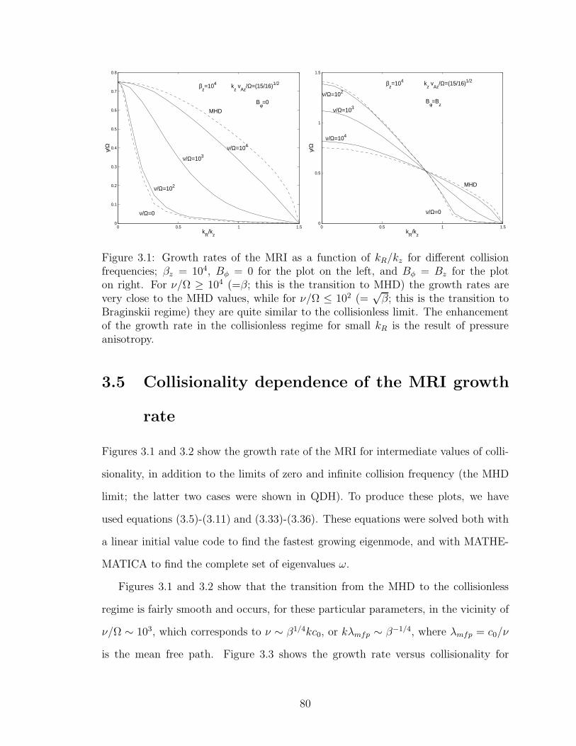
0 0.5 1 1.50

0.1

0.2

0.3

0.4

0.5

0.6

0.7

0.8

kR

/kz

γ/Ω

MHD

ν/Ω=104

ν/Ω=103

ν/Ω=102

ν/Ω=0

βz=104 k

z v

Az/Ω=(15/16)1/2

Bφ=0

0 0.5 1 1.50

0.5

1

1.5

kR

/kz

γ/Ω

MHD

ν/Ω=104

ν/Ω=103

ν/Ω=102

ν/Ω=0

βz=104 k

z v

Az/Ω=(15/16)1/2

Bφ=Bz

Figure 3.1: Growth rates of the MRI as a function of kR/kz for different collisionfrequencies; βz = 104, Bφ = 0 for the plot on the left, and Bφ = Bz for the ploton right. For ν/Ω ≥ 104 (=β; this is the transition to MHD) the growth rates arevery close to the MHD values, while for ν/Ω ≤ 102 (=

√β; this is the transition to

Braginskii regime) they are quite similar to the collisionless limit. The enhancementof the growth rate in the collisionless regime for small kR is the result of pressureanisotropy.

3.5 Collisionality dependence of the MRI growth

rate

Figures 3.1 and 3.2 show the growth rate of the MRI for intermediate values of colli-

sionality, in addition to the limits of zero and infinite collision frequency (the MHD

limit; the latter two cases were shown in QDH). To produce these plots, we have

used equations (3.5)-(3.11) and (3.33)-(3.36). These equations were solved both with

a linear initial value code to find the fastest growing eigenmode, and with MATHE-

MATICA to find the complete set of eigenvalues ω.

Figures 3.1 and 3.2 show that the transition from the MHD to the collisionless

regime is fairly smooth and occurs, for these particular parameters, in the vicinity of

ν/Ω ∼ 103, which corresponds to ν ∼ β1/4kc0, or kλmfp ∼ β−1/4, where λmfp = c0/ν

is the mean free path. Figure 3.3 shows the growth rate versus collisionality for

80

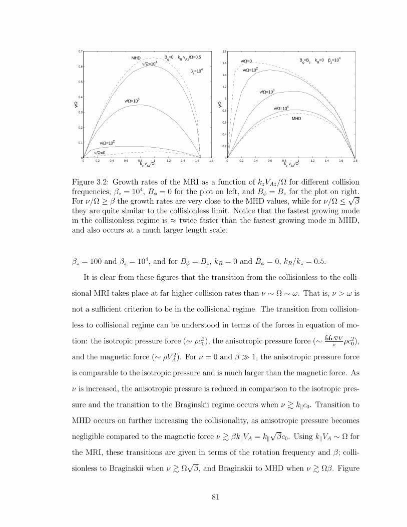
0 0.2 0.4 0.6 0.8 1 1.2 1.4 1.6 1.80

0.1

0.2

0.3

0.4

0.5

0.6

0.7

γ/Ω

kz v

Az/Ω

Bφ=0 kR

vAz

/Ω=0.5

βz=104

MHD ν/Ω=104

ν/Ω=103

ν/Ω=102

ν/Ω=0

0 0.2 0.4 0.6 0.8 1 1.2 1.4 1.6 1.80

0.2

0.4

0.6

0.8

1

1.2

1.4

1.6

1.8

γ/Ω

kz v

Az/Ω

Bφ=Bz k

R=0 β

z=104 ν/Ω=0

ν/Ω=102

ν/Ω=103

ν/Ω=104

MHD

Figure 3.2: Growth rates of the MRI as a function of kzVAz/Ω for different collisionfrequencies; βz = 104, Bφ = 0 for the plot on left, and Bφ = Bz for the plot on right.For ν/Ω ≥ β the growth rates are very close to the MHD values, while for ν/Ω ≤

√β

they are quite similar to the collisionless limit. Notice that the fastest growing modein the collisionless regime is ≈ twice faster than the fastest growing mode in MHD,and also occurs at a much larger length scale.

βz = 100 and βz = 104, and for Bφ = Bz, kR = 0 and Bφ = 0, kR/kz = 0.5.

It is clear from these figures that the transition from the collisionless to the colli-

sional MRI takes place at far higher collision rates than ν ∼ Ω ∼ ω. That is, ν > ω is

not a sufficient criterion to be in the collisional regime. The transition from collision-

less to collisional regime can be understood in terms of the forces in equation of mo-

tion: the isotropic pressure force (∼ ρc20), the anisotropic pressure force (∼ bb:∇Vν

ρc20),

and the magnetic force (∼ ρV 2A). For ν = 0 and β ≫ 1, the anisotropic pressure force

is comparable to the isotropic pressure and is much larger than the magnetic force. As

ν is increased, the anisotropic pressure is reduced in comparison to the isotropic pres-

sure and the transition to the Braginskii regime occurs when ν & k‖c0. Transition to

MHD occurs on further increasing the collisionality, as anisotropic pressure becomes

negligible compared to the magnetic force ν & βk‖VA = k‖√βc0. Using k‖VA ∼ Ω for

the MRI, these transitions are given in terms of the rotation frequency and β; colli-

sionless to Braginskii when ν & Ω√β, and Braginskii to MHD when ν & Ωβ. Figure

81

0 2 4 6 8 100

0.5

1

1.5

ν/Ωβ3/4

γ/Ω

β=104, kR

/kz=0, Bφ=B

z

β=100, kR

/kz=0, Bφ=B

z

β=100, kR

/kz=0.5, Bφ=B

z

β=104, kR

/kz=0.5, Bφ=0

Figure 3.3: Variation of the MRI growth rate with collisionality for kR = 0, Bφ = Bz

(top curves) and kR/kz = 0.5, Bφ = 0 (bottom curves). Collisions isotropize thedistribution function and can increase the growth rate in some regimes and decreaseit in others. Solid lines correspond to β = 104 and dotted lines to β = 102.

3.3 clearly shows that the transition from collisionless to MHD regime occurs roughly

when ν & Ωβ3/4, the geometric mean of the two transition collision frequencies.

At high β(≫ 1), the Alfven and MRI frequencies are small compared to the

sound wave frequency, and there exists a regime ω ≪ ν . k‖c0 where the collisionless

results still hold, despite the collision time being shorter than the growth rate of the

mode. Physically, this is because in order to wipe out the pressure anisotropy, that is

crucial to the MRI in a collisionless plasma (see QDH), the collision frequency must

be greater than the sound wave frequency, rather than the (much slower) growth

rate of the mode. This can also be seen by comparing Figures 3.1 and 3.2 with the

corresponding figures in QDH: the effect of increasing collisions (decreasing pressure

anisotropy) is similar to that of decreasing βz (decreasing pressure force relative to

magnetic forces). From the point of view of Snyder et al.’s fluid approach, the weak

dependence of growth rate on collisionality, even if ν is as large as ω, is because the

terms proportional to ω and ν in Eqs. (3.33) and (3.34) are both much smaller than

82

the dominant terms involving convection, heat conduction, and magnetic forces. So

the relative magnitudes of ω and ν are not that important, and it is not until ν is large

enough to be relevant in Eqs. 3.33-3.36, that collisional effects become noticeable.

Figure 3.4 shows the complete spectrum of eigenmode frequencies as kz is var-

ied, including the propagating and damped modes, in addition to the unstable MRI

branch. We show all the waves present in collisionless Landau fluid and MHD cal-

culations for a general choice of wavenumbers and a moderate βz(= 10). The MRI

is operational at lower kz, while at high kz the eigenfrequencies eventually approach

the uniform plasma limit.

Focusing first on the MHD solutions at high kz, we see the standard set of 3 MHD

waves: in order of descending frequency these are the fast magnetosonic wave, the

shear Alfven wave, and the slow wave. Eqs. 3.5-3.11 with an MHD adiabatic pressure

equation ωδp = p0k · δv is a set of 8 equations with 8 eigenvalues for ω. The standard

3 MHD waves provide 6 of the eigenvalues (±ω for oppositely propagating waves).

The remaining roots are zero frequency modes (not shown in the plot). One is an

entropy mode, corresponding to δρ/ρ0 = −δT/T0 so that δp = 0. The other solution

corresponds to an unphysical fluctuation that violates ∇ ·B = 0, which is eliminated

by imposing the proper initial condition ∇ ·B = 0. At lower kz in the MHD plots in

Figure 3.4, the slow mode is destabilized to become the MRI, as discussed in [16].

Turning next to the collisionless limit in Figure 3.4, there are two roots plotted in

addition to the three “MHD-like” modes; this is because the single pressure equation

of MHD is replaced by separate equations for the parallel and perpendicular pressure,

so that there are now two entropy-like modes, both of which have non-zero frequen-

cies but which are also strongly damped by collisionless heat conduction (which is

neglected in MHD).4

4We should point out that while our equations using the 3+1 Landau-fluid closure approximationshave 8 eigenfrequencies, the equations using the more accurate 4+2 Landau-fluid closure approx-imations have 10 eigenfrequencies, with 2 additional strongly damped roots. If the exact kineticresponse were used, one would find an infinite number of strongly damped eigenmodes because the

83

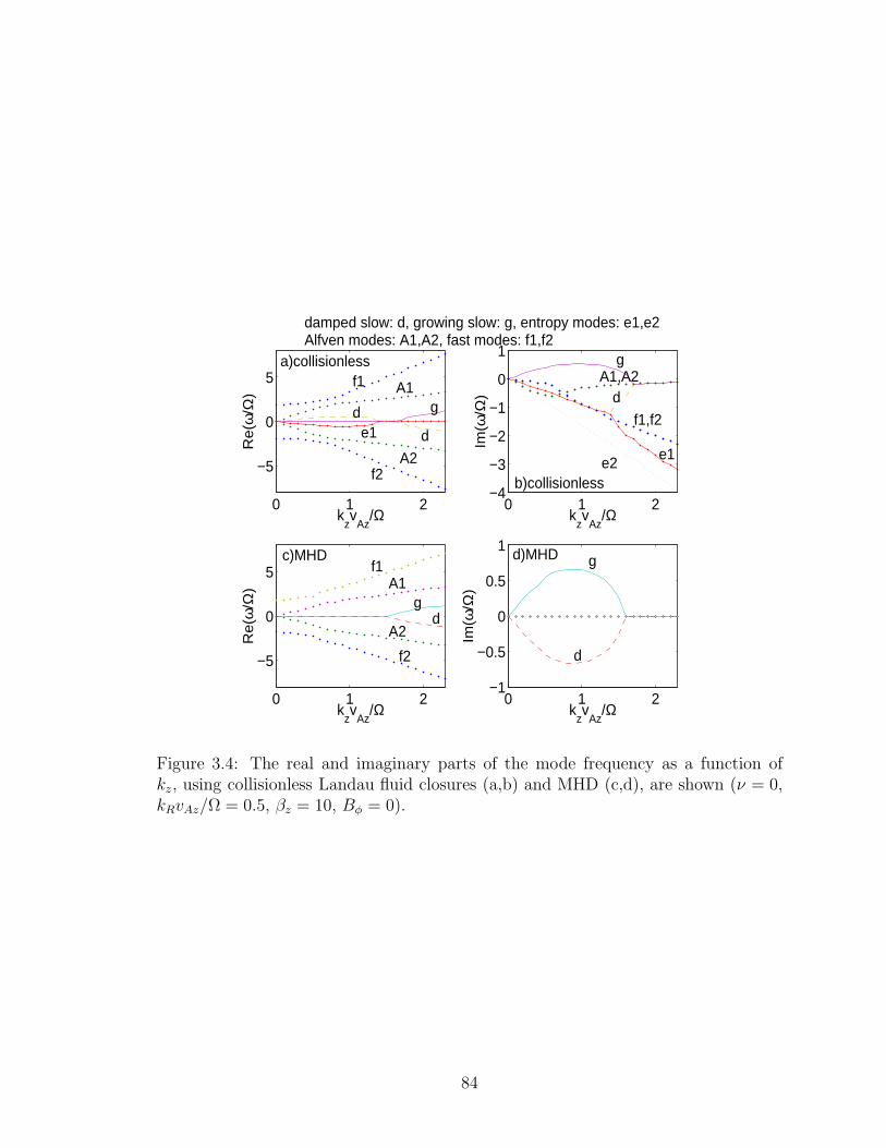
0 1 2

−5

0

5

kzv

Az/Ω

Re

(ω/Ω

)

0 1 2−4

−3

−2

−1

0

1

kzv

Az/Ω

Im(ω

/Ω)

0 1 2

−5

0

5

kzv

Az/Ω

Re

(ω/Ω

)

0 1 2−1

−0.5

0

0.5

1

kzv

Az/Ω

Im(ω

/Ω)

damped slow: d, growing slow: g, entropy modes: e1,e2Alfven modes: A1,A2, fast modes: f1,f2

f1 A1

d g

e1 d

A2 f2

g A1,A2

d

f1,f2

e2 e1

a)collisionless

b)collisionless

c)MHD d)MHD f1

A1 g

d A2

f2

g

d

Figure 3.4: The real and imaginary parts of the mode frequency as a function ofkz, using collisionless Landau fluid closures (a,b) and MHD (c,d), are shown (ν = 0,kRvAz/Ω = 0.5, βz = 10, Bφ = 0).

84

The fast, Alfven, and slow waves in the collisionless calculation can again be

identified in order of decreasing (real) frequency at high kz. At lower kz, one of

the slow modes becomes destabilized to become the MRI, as in MHD. Unlike in

MHD, however, the fast magnetosonic waves are strongly Landau damped since the

resonance condition ω ∼ k‖c0 is easily satisfied. In addition, it is interesting to note

that both the shear Alfven and slow waves have some collisionless damping at the

highest kz used in this plot, though the damping will approach zero for very high

kz. In a uniform plasma the shear Alfven wave is undamped unless its wavelength

is comparable to the proton Larmor radius or its frequency is comparable to the

proton cyclotron frequency (neither of which is true for the modes considered here).

By contrast, the slow mode is strongly damped unless k⊥ ≪ k‖ (because δv‖ ∝

(k⊥/k‖) ≪ c0 in this regime; e.g., [18, 60]). The damping of small kz shear Alfven

waves in Figure 3.4 is because our background plasma is rotating so the uniform-

plasma modes are mixed together. Thus the well-known dissipation of the slow mode

by transit-time damping also leads to damping of what we identify as the shear Alfven

wave (based on its high kz properties).

3.6 Summary and Discussion

In this chapter we have extended the linear, axisymmetric, kinetic magnetorotational

instability (MRI) calculation of QDH to include the effect of collisions. As the collision

frequency is increased, the MRI transitions from collisionless to Braginskii regime (ν &

Ω√β), and eventually to the MHD regime (ν & Ωβ). Interestingly, the collisionless

MRI results hold not only if ν ≪ ω, but even when ω ≪ ν ≪ k‖c0. This intermediate

regime can exist in β & 1 plasmas because the MRI growth rate is slow compared

to the sound wave frequency, ω ∼ k‖VA = k‖c0√

2/β ≪ k‖c0. The fastest growing

Z(ζ) function is transcendental. These strongly damped modes are related to “ballistic modes” andtransients in the standard analysis of Landau damping.

85

collisionless MRI mode is ≈ twice faster than the fastest growing MHD mode, and

occurs at a much larger length scale; thus, MRI in the collisionless regime can result

in fast MHD dynamo at large scales (not much smaller than the disk height scale).

If we consider the application of our results to accretion flows, the collisionless limit

will be applicable so long as ν/Ω .√β. This condition is amply satisfied for proton-

proton and proton-electron collisions in all hot radiatively inefficient accretion flow

models (see Table 1.2), suggesting that the collisionless limit is always appropriate.

However, high frequency waves such as ion-cyclotron waves can isotropize the proton

distribution function and thus provide an effective “collision” term crudely analogous

to the one considered here (see Subsection 4.2.2). In the drift kinetic limit, when

the Larmor radius is small compared to the dynamical length scales, the adiabatic

invariant µ = p⊥/B is conserved. Nonlinear simulations described in Chapter 4 show

that the MRI results in fast growth of magnetic fields resulting in an anisotropic

plasma (p⊥ > p⊥). Fairly large pressure anisotropies (∆p/p ∼ (a few)/β) are created

at the dynamical timescales and small scale instabilities—mirror and ion-cyclotron—

are excited. Pressure isotropization due to these instabilities imposes an MHD like

dynamics on a formally collisionless plasma. However, selective heating of resonant

electrons and ions may result in different electron and ion temperatures, and spectral

signatures different from MHD.

One might anticipate that the linear differences between the collisionless and col-

lisional MRI highlighted here and in QDH will imply differences in the nonlinear

turbulent state in hot accretion flows (see, e.g., [83, 95] for global MHD simula-

tions of such flows). Not only are there differences in the linear growth rates of the

instability that drives turbulence, but the spectrum of damped modes is also very

different. In particular, in the kinetic regime there exist modes at all scales in |k|

that are subject to Landau/Barnes collisionless damping, while in the MHD regime

the only sink for turbulent energy is due to viscosity/resistivity at very small scales

86

(very high |k|). Indeed, as we have shown, even long wavelength Alfven waves can

be damped by collisionless effects because of the mixture of uniform-plasma modes

in the differentially rotating accretion flow (Figure 3.4). Whether these differences

are important or not may depend on how efficiently nonlinearities couple energy into

the damped modes. These could modify the nonlinear saturated turbulent spectrum

(e.g., the efficiency of angular momentum transport) or the fraction of electron vs.

ion heating (the heating may also be anisotropic), which in turn determines the basic

observational signatures of hot accretion flows (the accretion rate and the radiative

efficiency). One approach for investigating nonlinear collisionless effects would be to

extend existing MHD codes to include anisotropic pressure, the fluid closure approxi-

mations for kinetic effects [180], and the BGK collision operator considered here. By

varying the collision frequency, one can then scan from the collisionless kinetic to the

collisional MHD regime, and assess any differences in the nonlinear turbulent state.

The nonlinear simulations of the collisionless MRI, based on Landau fluid closure for

heat fluxes, are described in the next chapter.

87

Chapter 4

Nonlinear Simulations of kinetic

MRI

In this chapter we describe local shearing box simulations of turbulence driven by

the magnetorotational instability (MRI) in a collisionless plasma. Collisionless effects

may be important in radiatively inefficient accretion flows, such as near the black

hole in the Galactic center (see Section 1.4). The ZEUS MHD code is modified to

evolve an anisotropic pressure tensor. A Landau-fluid closure approximation is used

to calculate heat conduction along magnetic field lines. The anisotropic pressure

tensor provides a qualitatively new mechanism for transporting angular momentum

in accretion flows (in addition to the Maxwell and Reynolds stresses). We estimate

limits on the pressure anisotropy due to pitch angle scattering by kinetic instabilities.

Such instabilities provide an effective “collision” rate in a collisionless plasma and

lead to more MHD-like dynamics. We find that the MRI leads to efficient growth of

the magnetic field in a collisionless plasma, with saturation amplitudes comparable

to those in MHD. In the saturated state, the anisotropic stress is comparable to

the Maxwell stress, implying that the rate of angular momentum transport may be

moderately enhanced in a collisionless plasma. More importantly, heating due to

88

anisotropic stress is comparable to the numerical energy loss in updating magnetic

fields; this can have important consequences for electron and ion heating.

4.1 Introduction

Following the seminal work of Balbus and Hawley [14], numerical simulations have

demonstrated that magnetohydrodynamic (MHD) turbulence initiated by the mag-

netorotational instability (MRI) is an efficient mechanism for transporting angular

momentum in accretion disks (see Section 1.3 for a review). For a broad class of as-

trophysical accretion flows, however, the MHD assumption is not directly applicable.

In particular, in radiatively inefficient accretion flow (RIAF) models for accretion onto

compact objects, the accretion proceeds via a hot, low density, collisionless plasma

with the proton temperature larger than the electron temperature [140, 156] (see Sec-

tion 1.4 for a review). In order to maintain such a two-temperature flow the plasma

must be collisionless, with the Coulomb mean-free path many orders of magnitude

larger than the system size (see Table 1.2 for plasma parameters in Sgr A∗). Moti-

vated by the application to RIAFs, this chapter studies the nonlinear evolution of the

collisionless MRI in the local shearing box limit.

Quataert, Dorland, & Hammett (2001; hereafter QDH) and Sharma, Hammett,

& Quataert (2003; hereafter SHQ) showed that the linear dynamics of the MRI in a

collisionless plasma can be quite different from that in MHD (see Chapter 3). The

maximum growth rate is a factor of ≈ 2 larger and, perhaps more importantly, the

fastest growing modes can shift to much longer wavelengths, giving direct amplifica-

tion of long wavelength modes. Dynamical instability exists even when the magnetic

tension forces are negligible because of the anisotropic pressure response in a collision-

less plasma. In related work using Braginskii’s anisotropic viscosity, the collisionless

MRI is studied as the “magnetoviscous” instability [12, 96].

89

We are interested in simulating the dynamics of a collisionless plasma on length-

scales (∼ disk height) and time-scales (∼ orbital period) that are very large compared

to the microscopic plasma scales (such as the Larmor radius and the cyclotron pe-

riod). Since the ratio of the size of the accretion flow to the proton Larmor radius is

∼ 108 for typical RIAF models (see Table 1.2), direct particle methods such as PIC

(particle in a cell), which need to resolve both of these scales, are computationally

challenging and require simulating a reduced range of scales. Instead, we use a fluid-

based method to describe the large-scale dynamics of a collisionless plasma (“kinetic

MHD,” described in Section 2.3). The key differences with respect to MHD are that

the pressure is a tensor rather than a scalar, anisotropic with respect to the direction

of the local magnetic field, and that there are heat fluxes along magnetic field lines

(related to Landau damping and wave-particle interactions). The drawback of our

fluid-based method is, of course, that there is no exact expression for the heat fluxes

if only a few fluid moments are retained in a weakly collisional plasma (the “closure

problem”). We use results from Snyder, Hammett, & Dorland (1997; hereafter SHD)

who have derived approximations for the heat fluxes in terms of nonlocal parallel

temperature and magnetic field gradients. These heat flux expressions can be shown

to be equivalent to multi-pole Pade approximations to the Z-function involved in

Landau damping (see Section 2.4). This approach can be shown to converge as more

fluid moments of the distribution function are kept [77], just as an Eulerian kinetic

algorithm converges as more grid points in velocity space are kept. These fluid-based

methods have been applied with reasonable success to modeling collisionless turbu-

lence in fusion plasmas, generally coming within a factor of 2 of more complicated

kinetic calculations in strong turbulence regimes [52, 147, 77, 173], though there can

be larger differences in weak turbulence regimes [77, 52]. The simulations we report

here use an even simpler local approximation to the heat flux closures than those

derived in [180] (see “the crude closure” in Section 2.4). While not exact, these clo-

90

sure approximations allow one to begin to investigate kinetic effects with relatively

fast modifications of fluid codes; whereas, solving the full drift kinetic equation (see

Section 2.2) is considerably slower and requires code development and testing from

scratch.

In a collisionless plasma the magnetic moment, µ = v2⊥/2B, is an adiabatic invari-

ant. Averaged over velocity space, this leads to conservation of 〈µ〉 = p⊥/(ρB). As

a result, pressure anisotropy with p⊥ > p‖ is created as the MRI amplifies the mag-

netic field in the accretion flow. This pressure anisotropy creates an anisotropic stress

(like a viscosity!) which can be as important for angular momentum transport as the

magnetic stress. It is interesting to note that for cold disks, the mean free path is neg-

ligible compared to the disk height resulting in a viscosity insufficient to account for

efficient transport; but hot, thick accretion flows are collisionless with large viscosity,

and viscous stress is quite efficient in transporting angular momentum. However, it

is important to emphasize that an anisotropic viscosity in a collisionless, magnetized

plasma is very different from an isotropic viscosity (since viscosity perpendicular to

the field lines is vanishingly small). Although, the Reynolds number (Re ≡ V L/ηV )

based on parallel viscosity is small, O(1), the plasma is turbulent; this would not be

true if the Reynolds number based on an isotropic viscosity is so small.

The pressure anisotropy cannot, however, grow without bound because high fre-

quency waves and kinetic microinstabilities feed on the free energy in the pressure

anisotropy, effectively providing an enhanced rate of collisions that limit the pressure

tensor anisotropy (leading to more MHD-like dynamics in a collisionless plasma). We

capture this physics by using a subgrid model to restrict the allowed amplitude of

the pressure anisotropy. This subgrid model (described in §2.3) is based on existing

linear and nonlinear studies of instabilities driven by pressure anisotropy [80, 69].

The remainder of this paper is organized as follows. We begin with Kulsrud’s

formulation of kinetic MHD (KMHD) and our closure model for the heat fluxes in

91

a collisionless plasma. We also include a linear analysis of the MRI in the presence

of a background pressure anisotropy and describe limits on the pressure anisotropy

set by kinetic instabilities. Next, we describe our modifications to the ZEUS code to

model kinetic effects. We present our primary results on the nonlinear evolution of

the MRI in a collisionless plasma. At the end we discuss these results, their astro-

physical implications, and future work required to understand the global dynamics of

collisionless accretion disks.

4.2 Governing equations

In the limit that all fluctuations of interest are at scales larger than the proton Larmor

radius and have frequencies much smaller than the proton cyclotron frequency, a

collisionless plasma can be described by the following magnetofluid equations [110,

180] (see Section 2.3 for details):

∂ρ

∂t+ ∇ · (ρV) = 0, (4.1)

ρ∂V

∂t+ ρ (V · ∇)V =

(∇× B) × B

4π−∇ ·P + Fg, (4.2)

∂B

∂t= ∇× (V × B) , (4.3)

P = p⊥I +(

p‖ − p⊥)

bb = p⊥I + Π, (4.4)

where ρ is the mass density, V is the fluid velocity, B is the magnetic field, Fg is

the gravitational force, b = B/|B| is a unit vector in the direction of the magnetic

field, and I is the unit tensor. In equation (4.3) an ideal Ohm’s law is used, neglecting

resistivity. In equation (4.4), P is the pressure tensor with different perpendicular (p⊥)

and parallel (p‖) components with respect to the background magnetic field, and

Π = bb(p‖− p⊥) is the anisotropic stress tensor. (Note that Π is not traceless in the

convention used here.) P should in general be a sum over all species but in the limit

92

where ion dynamics dominate and electrons just provide a neutralizing background,

the pressure can be interpreted as the ion pressure. This is the case for hot accretion

flows in which Tp ≫ Te.

The exact pressures p‖ and p⊥ can be rigorously determined by taking moments

of the drift kinetic equation (see Section 2.2),

∂fs

∂t+ (v‖b + VE) · ∇fs +

[

−b · DVE

Dt− µb · ∇B +

es

ms

(

E‖ +Fg‖

es

)]

∂fs

∂v‖= C(fs),

(4.5)

which is the asymptotic expansion of the Vlasov equation for the distribution function

fs(x, µ, v‖, t) for species ‘s’ with mass ms and charge es in the limit ρs/L≪ 1, ω/Ωs ≪

1, where ρs and Ωs are the gyroradius and gyrofrequency, respectively. In equation

(4.5), VE = c(E × B)/B2 is the perpendicular drift velocity, µ = (v⊥ − VE)2/2B

is the magnetic moment (a conserved quantity in the absence of collisions), Fg‖ is

the component of the gravitational force parallel to the direction of the magnetic

field, and D/Dt = ∂/∂t+ (v‖b + VE) · ∇ is the particle Lagrangian derivative in the

phase space. The fluid velocity V = VE + bV‖, so the E × B drift is determined

by the perpendicular component of equation (4.2). Other drifts such as grad B,

curvature, and gravity ×B drifts are higher order in the drift kinetic ordering and

do not appear in this equation. In equation (4.5), C(fs) is the collision operator to

allow for generalization to collisional regimes. Collisions can also be used to mimic

rapid pitch angle scattering due to high frequency waves that break µ invariance.

The parallel electric field is determined by E‖ =∑

s(es/ms)b · ∇ ·Ps/∑

s(nse2s/ms),

which insures quasineutrality (see Subsection 2.4.1).

Separate equations of state for the parallel and perpendicular pressures can be

obtained from the moments of the drift kinetic equation [48]. Neglecting the collision

93

term these are:

ρBD

Dt

(

p⊥ρB

)

= −∇ · q⊥ − q⊥∇ · b, (4.6)

ρ3

B2

D

Dt

(

p‖B2

ρ3

)

= −∇ · q‖ + 2q⊥∇ · b, (4.7)

where D/Dt = ∂/∂t + V · ∇ is the fluid Lagrangian derivative and q‖,⊥ = q‖,⊥b are

the heat fluxes (flux of p‖ and p⊥) parallel to the magnetic field. The equation for

the magnetic moment density ρ〈µ〉 = p⊥/B can be written in a conservative form:

∂

∂t

(p⊥B

)

+ ∇ ·(p⊥B

V)

= −∇ ·(q⊥B

b)

, (4.8)

If the heat fluxes are neglected (called the CGL or double adiabatic limit), as the

magnetic field strength (B) increases, p⊥ increases (p⊥ ∝ ρB), and p‖ decreases

(p‖ ∝ ρ3/B2). Integrating equation (4.8) over a finite periodic (even a shearing

periodic) box shows that 〈p⊥/B〉 is conserved, where 〈〉 denotes a volume average.

This implies that even when q‖,⊥ 6= 0, p⊥ increases in a volume averaged sense as the

magnetic energy in the box increases. This means that that for a collisionless plasma,

pressure anisotropy p⊥ > (<) p‖ is created as a natural consequence of processes that

amplify (reduce) B. This pressure anisotropy is crucial for understanding magnetic

field amplification in collisionless dynamos.

To solve the set of equations (4.1-4.4), (4.6-4.7) in a simple fluid based formalism,

we require expressions for q‖ and q⊥ in terms of lower order moments. No simple,

exact expressions for q‖ and q⊥ exist for nonlinear collisionless plasmas. Although

simple, the double adiabatic or CGL approximation (where q‖ = q⊥ = 0) does not

capture key kinetic effects such as Landau damping. In the moderately collisional

limit (ρi < mean free path < system size), where the distribution function is not very

different from a local Maxwellian, one can use the Braginskii equations to describe

94

anisotropic transport ([37]; see [10, 12] for astrophysical applications). However, in

the hot RIAF regime, the mean free path is often much larger than the system size and

the Braginskii equations are not formally applicable, though they are still useful as a

qualitative indication of the importance of kinetic effects. The collisional limit of the

kinetic MHD equations can be shown to recover the dominant anisotropic heat flux

and viscosity tensor of Braginskii (see Subsection 2.5.1). The local approximation to

kinetic MHD that we use here leads to equations that are similar in form to Braginskii

MHD, but with separate dynamical equations for parallel and perpendicular pressures.

We also add models for enhanced pitch angle scattering by microinstabilities, which

occur at very small scales and high frequencies beyond the range of validity of standard

kinetic MHD. 1

Hammett and collaborators have developed approximate fluid closures (called Lan-

dau fluid closure) for collisionless plasmas [79, 78, 180] that capture kinetic effects

such Landau damping. SHD [180] give the resulting expressions for parallel heat

fluxes (q‖, q⊥) to be used in equations (4.6) and (4.7). Landau closures are based

on Pade approximations to the full kinetic plasma dispersion function that reproduce

the correct asymptotic behavior in both the adiabatic (ω/k‖c‖ ≫ 1) and isother-

mal (ω/k‖c‖ ≪ 1) regimes (and provide a good approximation in between), where

ω is the angular frequency, k‖ is the wavenumber parallel to the magnetic field, and

c‖ =√

p‖/ρ is the parallel thermal velocity of the particles. In Fourier space, the

linearized heat fluxes can be written as equations (39) & (40) in SHD,

q‖ = −√

8

πρ0c‖0

ik‖(

p‖/ρ)

|k‖|, (4.9)

q⊥ = −√

2

πρ0c‖0

ik‖ (p⊥/ρ)

|k‖|+

√

2

πc‖0p⊥0

B0

(

1 − p⊥0

p‖0

)

ik‖B

|k‖|, (4.10)

1This would also be needed when using Braginskii equations, because they are not necessar-ily well posed in situations where the anisotropic stress tensor can drive arbitrarily small scaleinstabilities[170].

95

where ‘0′ subscripts indicate equilibrium quantities. Real space expressions are some-

what more cumbersome and are given by convolution integrals (see Section 2.4)

q‖ = −(

2

π

)3/2

n0c‖0

∫ ∞

0

δz′T‖(z + z′) − T‖(z − z′)

z′, (4.11)

q⊥ = −(

2

π3

)1/2

n0c‖0

∫ ∞

0

δz′T⊥(z + z′) − T⊥(z − z′)

z′

+

(

2

π3

)1/2

c‖0

(

1 − p⊥0

p‖0

)

p⊥0

B0×∫ ∞

0

δz′B(z + z′) − B(z − z′)

z′, (4.12)

where n0 is the number density, T‖ = p‖/n, and T⊥ = p⊥/n are the parallel and

perpendicular temperatures, and z′ is the spatial variable along the magnetic field line.

In the previous chapter (based on [176]) we have shown that these fluid closures for the

heat fluxes accurately reproduce the kinetic linear Landau damping rate for all MHD

modes (slow, Alfven, fast and entropy modes). The growth rate of the MRI using the

Landau closure model is also very similar to that obtained from full kinetic theory.

As noted in the introduction, in addition to reproducing linear modes/instabilities,

Landau fluid closures have also been used to model turbulence in fusion plasmas with

reasonable success.

These closure approximations were originally developed for turbulence problems

in fusion energy devices with a strong guide magnetic field, where the parallel dynam-

ics is essentially linear and FFTs could be easily used to quickly evaluate the Fourier

expressions above. In astrophysical problems with larger amplitude fluctuations and

tangled magnetic fields, evaluation of the heat fluxes become somewhat more compli-

cated. One could evaluate the convolution expressions, equations (4.11) and (4.12)

(with some modest complexity involved in writing a subroutine to integrate along

magnetic field lines), leading to a code with a computational time Tcpu ∝ N3xN‖,

where N3x is the number of spatial grid points and N‖ is the number of points kept

in the integrals along field lines. (In some cases, it may be feasible to map the fluid

96

quantities to and from a field-line following coordinate system so that FFTs can re-

duce this to Tcpu ∝ N3x logN‖.) While this is more expensive than simple MHD where

Tcpu ∝ N3x , it could still represent a savings over a direct solution of the drift kinetic

equation, which would require Tcpu ∝ N3xNv‖Nv⊥ , where Nv‖Nv⊥ is the number of grid

points for velocity space.2

As a first step for studying kinetic effects, in this paper we pick out a characteristic

wavenumber kL that represents the scale of collisionless damping and use a local

approximation for the heat fluxes in Fourier space (see the “crude closure for thermal

conduction” in Section 2.4), with a straightforward assumption about the nonlinear

generalization:

q‖ = −√

8

πρc‖

∇‖

(

p‖/ρ)

kL, (4.13)

q⊥ = −√

2

πρc‖

∇‖ (p⊥/ρ)

kL+

√

2

πc‖p⊥

(

1 − p⊥p‖

) ∇‖B

kLB. (4.14)

Note that this formulation of the heat flux is analogous to a Braginskii heat conduction

along magnetic field lines. For linear modes with |k‖| ∼ kL, these approximations will

of course agree with kinetic theory as well as the Pade approximations shown in SHD.

One can think of kL as approximately controlling the heat conduction rate, though

this does not necessarily affect the resulting Landau damping rate of a mode in a

monotonic way, since this sometimes exhibits impedance matching behavior,i.e., some

modes are weakly damped in both the small and large (isothermal) heat conduction

limits. We vary kL to investigate the sensitivity of our results to this parameter.

2On the other hand, an effective hyperdiffusion operator in velocity space may reduce the velocityresolution requirements, and recent direct kinetic simulations of turbulence in fusion devices havefound that often one does not need very high velocity resolution. This may make a direct solutionof the drift kinetic equation tractable for some astrophysical kinetic MHD problems. Furthermore,a direct solution of the drift kinetic equation involves only local operations, and thus is somewhateasier to parallelize than the convolution integrals.

97

4.2.1 Linear modes

Since pressure anisotropy arises as a consequence of magnetic field amplification in a

collisionless plasma, it is of interest to repeat the linear analysis of the collisionless

MRI done in Chapter 3, but with a background pressure anisotropy (p‖0 6= p⊥0). We

consider the simple case of a vertical magnetic field. This analysis provides a useful

guide to understanding some of our numerical results.

We linearize equations (4.1)-(4.4) for a differentially rotating disk (V0 = RΩ(R)φ)

with an anisotropic pressure about a uniform subthermal vertical magnetic field (B0 =

Bzz). We assume that the background (unperturbed) plasma is described by a bi-

Maxwellian distribution (p‖0 6= p⊥0). We also assume that the perturbations are

axisymmetric, of the form exp[−iωt+ik · x] with k = kRR+kzz. Writing ρ = ρ0+δρ,

B = B0 + δB, p⊥ = p⊥0 + δp⊥, p‖ = p‖0 + δp‖, working in cylindrical coordinates

and making a |k|R ≫ 1 assumption, the linearized versions of equations (4.1)-(4.3)

become:

ωδρ = ρ0k · δv, (4.15)

−iωρ0δvR − ρ02Ωδvφ = −ikR

4πBzδBz

+ ikz

(

Bz

4π− (p‖0 − p⊥0)

Bz

)

δBR − ikRδp⊥, (4.16)

−iωρ0δvφ + ρ0δvRκ2

2Ω= ikz

(

Bz

4π− (p‖0 − p⊥0)

Bz

)

δBφ, (4.17)

−iωρ0δvz = −ikR

(

p‖0 − p⊥0

) δBR

Bz

− ikzδp‖, (4.18)

ωδBR = −kzBzδvR, (4.19)

ωδBφ = −kzBzδvφ − ikzBz

ω

dΩ

d lnRδvR, (4.20)

ωδBz = kRBzδvR, (4.21)

where κ2 = 4Ω2 + dΩ2/d lnR is the epicyclic frequency. Equations (4.15)-(4.21)

describe the linear modes of a collisionless disk with an initial pressure anisotropy

98

about a vertical magnetic field. This corresponds to the θ = π/2 case of Chapter

3, but with an anisotropic initial pressure. Equations (4.16) & (4.17) show that an

initial anisotropic pressure modifies the Alfven wave characteristics, so we expect a

background pressure anisotropy to have an important effect on the MRI. One way of

interpreting equations (4.16) & (4.17) is that p⊥ > p‖ (p‖ > p⊥) makes the magnetic

fields more (less) stiff; as a result, this will shift the fastest growing MRI mode to

larger (smaller) scales.

The linearized equations for the parallel and perpendicular pressure response are

given by Eqs. 3.33 and 3.34 from Chapter 3. We present them here for the sake of

completeness.

−iωδp‖ + p‖0ik · δv + ikzq‖ + 2p‖0ikzδvz = 0, (4.22)

−iωδp⊥ + 2p⊥0ik · δv + ikzq⊥ − p⊥0ikzδvz = 0, (4.23)

where the heat fluxes can be expressed in terms of lower moments using

q⊥ = −√

2

πc‖0

ikz

|kz|(δp⊥ − c2‖0δρ) +

√

2

πc‖0p⊥0

(

1 − p⊥0

p‖0

)

ikz

|kz|δB

Bz

, (4.24)

q‖ = −√

8

πc‖0

ikz

|kz|(δp‖ − c2‖0δρ), (4.25)

where c‖0 =√

p‖0/ρ0 and δB = |δB|.

Figure 4.1 shows the MRI growth rate as a function of pressure anisotropy for

two values of kR for β = 100. This figure shows that the fastest growing MHD mode

(kR = 0) is stabilized for (p⊥0 − p‖0)/p‖0 ∼ 4/β; modes with kR 6= 0 modes require

larger anisotropy for stabilization. For β ≫ 1, these results highlight that only a very

small pressure anisotropy is required to stabilize the fastest growing MRI modes.

Growth at large pressure anisotropies in Figure 4.1 for kR 6= 0 mode is because of

the mirror instability that is discussed below. The physical interpretation of the

99

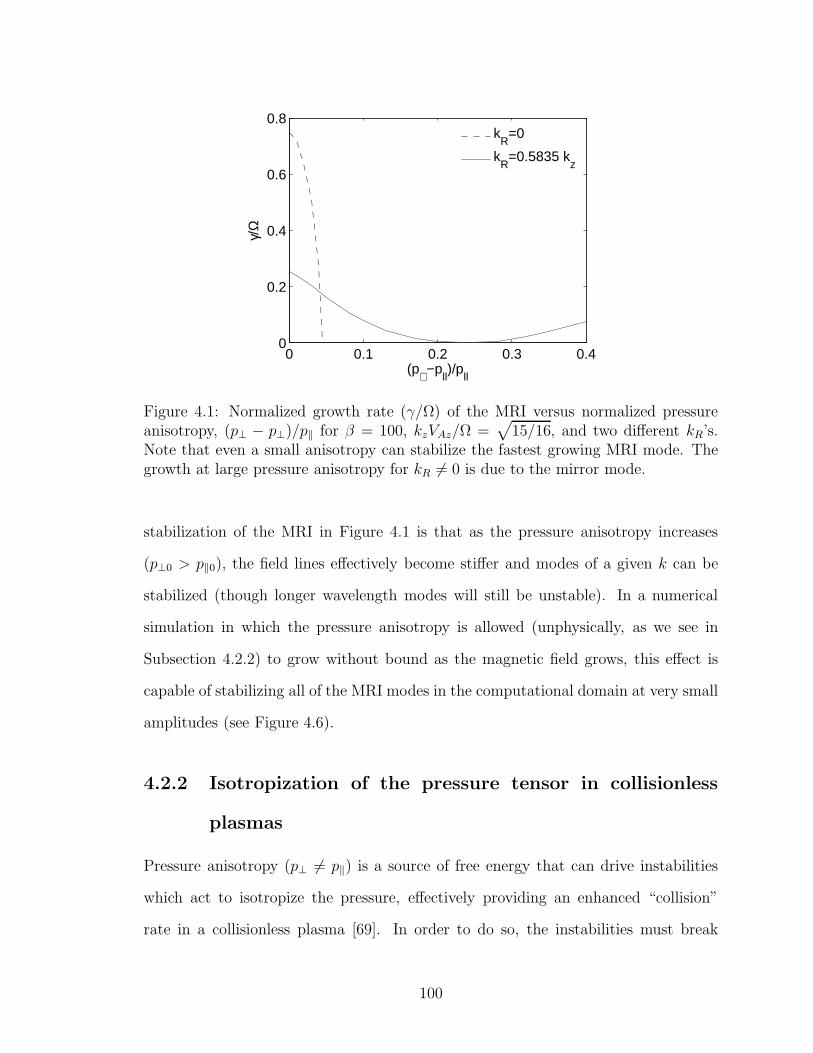
0 0.1 0.2 0.3 0.40

0.2

0.4

0.6

0.8

(p⊥ −pll)/p

ll

γ/Ω

kR

=0

kR

=0.5835 kz

Figure 4.1: Normalized growth rate (γ/Ω) of the MRI versus normalized pressureanisotropy, (p⊥ − p⊥)/p‖ for β = 100, kzVAz/Ω =

√

15/16, and two different kR’s.Note that even a small anisotropy can stabilize the fastest growing MRI mode. Thegrowth at large pressure anisotropy for kR 6= 0 is due to the mirror mode.

stabilization of the MRI in Figure 4.1 is that as the pressure anisotropy increases

(p⊥0 > p‖0), the field lines effectively become stiffer and modes of a given k can be

stabilized (though longer wavelength modes will still be unstable). In a numerical

simulation in which the pressure anisotropy is allowed (unphysically, as we see in

Subsection 4.2.2) to grow without bound as the magnetic field grows, this effect is

capable of stabilizing all of the MRI modes in the computational domain at very small

amplitudes (see Figure 4.6).

4.2.2 Isotropization of the pressure tensor in collisionless

plasmas

Pressure anisotropy (p⊥ 6= p‖) is a source of free energy that can drive instabilities

which act to isotropize the pressure, effectively providing an enhanced “collision”

rate in a collisionless plasma [69]. In order to do so, the instabilities must break

100

magnetic moment conservation, and thus must have frequencies comparable to the

cyclotron frequency and/or parallel wavelengths comparable to the Larmor radius.

Because of the large disparity in timescales between µ-breaking microinstabilities

and the MRI (ωmicro/Ω ∼ 108), one can envision the microinstabilities as providing

a “hard wall” limit on the pressure anisotropy; once the pressure anisotropy exceeds

the threshold value where microinstabilities are driven and cause rapid pitch angle

scattering, the pressure anisotropy nearly instantaneously reduces the anisotropy to

its threshold value (from the point of view of the global disk dynamics). In this

section we review the relevant instabilities that limit the pressure anisotropy in high

β collisionless plasmas—these are the firehose, mirror, and ion cyclotron instabilities.

We then discuss how we have implemented these estimated upper bounds on the

pressure anisotropy in our numerical simulations.

Maximum anisotropy for p‖ > p⊥

Plasmas with p‖ > p⊥ can be unstable to the firehose instability, whose dispersion

relation for parallel propagation is given by equation (2.12) of [100]:

ω2 − ωΩik2‖ρ

2i + Ω2

i k2‖ρ

2i

(

1 − p⊥p‖

− 2

β‖

)

= 0, (4.26)

where β‖ = 8πp‖/B2, ρi is the ion Larmor radius, Ωi is the ion cyclotron frequency,

and k‖ is the wavenumber parallel to the local magnetic field direction. Solving for ω

gives

ω = k2‖ρ

2i

Ωi

2± ik‖c‖0

(

1 − p⊥p‖

− 2

β‖−k2‖ρ

2i

4

)1/2

(4.27)

For long wavelengths, the firehose instability requires p‖ > p⊥ +B2/4π, and is essen-

tially an Alfven wave destabilized by the pressure anisotropy. The maximum growth

rate occurs when k2‖ρ

2i = 2(1 − p⊥/p‖ − 2/β‖) and is given by Ωi(1 − p⊥/p‖ − 2/β‖).

We use an upper limit on p‖ > p⊥ corresponding to 1 − p⊥/p‖ − 2/β‖ < 1/2, which

101

is an approximate condition for the growth of modes that will violate µ conservation

and produce rapid pitch angle scattering (when ω ∼ Ωi and k‖ρi ∼ 1).

Maximum anisotropy for p⊥ > p‖

For p⊥ > p‖ there are two instabilities that act to isotropize the pressure, the mirror

instability and the ion cyclotron instability [69]. A plasma is unstable to the mirror

instability when p⊥/p‖ − 1 > 1/β⊥, although as discussed below only for somewhat

larger anisotropies is magnetic moment conservation violated. Formally, a plasma

with any nonzero pressure anisotropy can be unstable to the ion cyclotron instability

[182]. However, there is an effective threshold given by the requirement that the

unstable modes grow on a timescale comparable to the disk rotation period.

The growth rate of the mirror instability is given by (Eq. (36) of [80])

γ =

(

2

π

)1/2(T⊥T‖

)3/2

k‖c⊥0

[

T⊥T‖

− 1 − 1

β⊥

(

1 +k2‖

k2⊥

)

exp(λ)

I0(λ) − I1(λ)

]

, (4.28)

where c⊥0 =√

p⊥/ρ, λ = (k‖c⊥0/Ωi)2, and I0 and I1 are modified Bessel functions of

order 0 and 1. Minimizing the growth rate with respect to k‖ and k⊥ gives equations

(43′) & (44′) of [80], which give the wavenumber for the fastest growing mirror mode,

k‖k⊥

=

√

(D − 1)

4, (4.29)

k⊥ρi =

√

(D − 1)

6, (4.30)

where D = β⊥(p⊥/p‖ − 1), β⊥ = 8πp⊥/B2. To estimate the pressure anisotropy at

which µ conservation is broken and thus pitch angle scattering is efficient, we calculate

D for which k‖ρi ∼ k⊥ρi ∼ 1. This implies D ≈ 7, or that µ conservation fails (and

102

pitch angle scattering occurs) if the pressure anisotropy satisfies

p⊥p‖

− 1 >7

β⊥. (4.31)

The ion cyclotron instability can be also be excited when p⊥ > p‖. Gary and col-

laborators have analyzed the ion cyclotron instability in detail through linear analysis

and numerical simulations [69, 67]. They calculate the pressure anisotropy required

for a given growth rate γ relative to the ion cyclotron frequency Ωi

p⊥p‖

− 1 >S ′

βp‖

(4.32)

where S ′ = 0.35 and p = 0.42 are fitting parameters quoted in equation (2) of [67]

for γ/Ωi = 10−4. Moreover, for γ ≪ Ωi the threshold anisotropy depends only very

weakly on the growth rate γ. As a result, equation (4.32) provides a reasonable

estimate of the pressure anisotropy required for pitch angle scattering by the ion

cyclotron instability to be important on a timescale comparable to the disk rotation

period.

4.2.3 Pressure anisotropy limits

Motivated by the above considerations, we require that the pressure anisotropy satisfy

the following inequalities in our simulations (at each grid point and at all times):

p⊥p‖

− 1 +2

β‖>

1

2, (4.33)

p⊥p‖

− 1 <2ξ

β⊥, (4.34)

p⊥p‖

− 1 < S

(

2

β‖

)1/2

, (4.35)

103

where S and ξ are constants described below. It is important to note that the fluid-

based kinetic theory utilized in this paper can correctly reproduce the existence and

growth rates of the firehose and mirror instabilities (though not the ion cyclotron

instability).3 However, it can only do so for long wavelength perturbations that con-

serve µ. The relevant modes for pitch angle scattering occur at the Larmor radius

scale, which is very small in typical accretion flows and is unresolved in our simula-

tions. For this reason we must impose limits on the pressure anisotropy and cannot

simultaneously simulate the MRI and the relevant instabilities that limit the pressure

anisotropy. The algorithm to impose the pressure anisotropy limits is explained in

Appendix C.2.

In Eq. 4.34, the parameter ξ determines the threshold anisotropy above which the

mirror instability leads to pitch angle scattering. A value of ξ = 3.5 was estimated

in Section 4.2.2. We take this as our fiducial value, but for comparison also describe

calculations with ξ = 0.5, which corresponds to the marginal state for the mirror

instability. We compare both models because the saturation of the mirror instability

is not well understood, particularly under the conditions appropriate to a turbulent

accretion disk. Eq. 4.35 is based on the pitch angle scattering model used by [26]

for simulations of magnetic reconnection in collisionless plasmas; following them we

choose S = 0.3. Eq. 4.35 with S = 0.3 gives results which are nearly identical (for

the typical range of β studied here) to the pressure anisotropy threshold for the ion

cyclotron instability discussed in Section 4.2.2 (Eq. 4.32).

In our simulations we find that for typical calculations, if ξ = 0.5 then Eq. 4.34

(the “mirror instability”) dominates the isotropization of the pressure tensor, while

if ξ = 3.5 then Eq. 4.35 (the “ion cyclotron instability”) dominates. We also find

that our results are insensitive to the form of the p‖ > p⊥ threshold (Eq. 4.33); e.g.,

3The double adiabatic limit (q⊥ = q‖ = 0) predicts an incorrect threshold and incorrect growthrates for the mirror instability [180]. Thus it is important to use the heat flux models described in§2 to capture the physics of the mirror instability.

104

simulations with 1−p⊥/p‖ < 2/β‖ (the marginal state of the firehose mode) instead of

equation (4.33) give nearly identical results. Fully kinetic simulations of the mirror,

firehose, and ion cyclotron instabilities will be useful for calibrating the pitch angle

scattering models used here.

4.3 Kinetic MHD simulations in shearing box

In this section we discuss the shearing box equations that we solve numerically, and

the modifications made to ZEUS to include kinetic effects.

4.3.1 Shearing box

The shearing box is based on a local expansion of the tidal forces in a reference frame

rotating with the disk (see HGB for details). A fiducial radius R0 in the disk is picked

out and the analysis is restricted to a local Cartesian patch such that Lx, Ly, Lz ≪ R0

(where x = r − R0, y = φ and z = z). In this paper only the radial component of

gravity is considered, and vertical gravity and buoyancy effects are ignored. We also

assume a Keplerian rotation profile. With these approximations, the equations of

Landau MHD (kinetic MHD combined with Landau closure for parallel heat fluxes)

105

in the shearing box are:

∂ρ

∂t+ ∇ · (ρV) = 0, (4.36)

∂V

∂t+ V · ∇V = −1

ρ∇(

p⊥ +B2

8π

)

+B · ∇B

4πρ− 1

ρ∇ ·Π

− 2Ω ×V + 3Ω2xx, (4.37)

∂B

∂t= ∇× (V ×B), (4.38)

∂p‖∂t

+ ∇ · (p‖V) + ∇ · q‖ + 2p‖b · ∇V · b− 2q⊥∇ · b = −2

3νeff (p‖ − p⊥),(4.39)

∂p⊥∂t

+ ∇ · (p⊥V) + ∇ · q⊥ + p⊥∇ · V − p⊥b · ∇V · b + q⊥∇ · b

= −1

3νeff(p⊥ − p‖), (4.40)

q‖ = −ρκ‖∇‖

(

p‖ρ

)

, (4.41)

q⊥ = −ρκ⊥∇‖

(

p⊥ρ

)

+ κmB · ∇B, (4.42)

where q‖ = q‖b and q⊥ = q⊥b are the heat fluxes parallel to the magnetic field, νeff

is the effective pitch-angle scattering rate (includes microinstabilities, see Subsection

4.2.2 and Appendix C.2), κ‖ and κ⊥ are the coefficients of heat conduction, and κm is

the coefficient in q⊥ due to parallel gradients in the strength of magnetic field [180].

The κm component of q⊥ that arises because of parallel magnetic field gradients is

important for correctly recovering the saturated state for the mirror instability in the

fluid limit, where (in steady state) q‖,⊥ ≈ 0 implies that T‖ is constant along the field

line, and T⊥ and magnetic pressure are anticorrelated.

106

Given our closure models, the coefficients for the heat fluxes are given by

κ‖ =8p‖ρ

1√

8πp‖ρkL + (3π − 8)νeff

, (4.43)

κ⊥ =p‖ρ

1√

π2

p‖ρkL + νeff

, (4.44)

κm =

(

1 − p⊥p‖

)

p⊥B2

κ⊥, (4.45)

where kL is the parameter that corresponds to a typical wavenumber characterizing

Landau damping (see “crude model of Landau damping” in Section 2.4). We consider

several values of kL to study the effect of Landau damping on different scales. In

particular, we consider kL = 0.5/δz, 0.25/δz, and 0.125/δz which correspond to

correctly capturing Landau damping on scales of 12δz, 24δz, 48δz, respectively, where

δz = Lz/Nz, Lz = 1 for all our runs, and Nz is the number of grid points in the z-

direction (taken be 27 and 54 for low and high resolution calculations, respectively).

Thus, kL = 0.25/δz corresponds to correctly capturing Landau damping for modes

with wavelengths comparable to the size of the box in the low resolution runs.

The term νeff in Eqs. 4.43 and 4.44 is an effective collision frequency which is

equal to the real collision frequency ν, as long as µ conservation is satisfied. However,

when the pressure anisotropy is large enough to drive microinstabilities that break µ

invariance , and enhance pitch angle scattering, then there is an increase in the effec-

tive collision frequency that decreases the associated conductivities. The expressions

for νeff are given in Eqs. C.12, C.15, and C.18 in Appendix C.2.

Shearing periodic boundary conditions appropriate to the shearing box are de-

scribed in [86]. Excluding Vy, all variables at the inner x- boundary are mapped to

sheared ghost zones at the outer boundary; a similar procedure applies for the inner

ghost zones. Vy has a jump of (3/2)ΩLx across the box while applying the x- shearing

boundary conditions, to account for the background shear in Vy.

107

4.3.2 Numerical methods

We have used the shearing box version of the ZEUS MHD code [185, 186], and

modified it to include kinetic effects. The ZEUS code is a time explicit, operator

split, finite difference algorithm on a staggered mesh, i.e., scalars and the diagonal

components of second rank tensors are zone centered, while vectors are located at

zone faces, and pseudovectors and offdiagonal components of second rank tensors are

located at the edges. The location of different variables on the grid is described in

detail in Appendix C.1. Appendix C.1.1 describes how we choose the time step δt

to satisfy the Courant condition (which is modified by pressure anisotropy and heat

conduction). We also require that the choice of δt maintain positivity of p‖ and p⊥.

Implementation of the shearing box boundary conditions is described in [86]. One

can either apply boundary conditions on the components of B or the EMFs (whose

derivatives give B). We apply shearing periodic boundary conditions on the EMFs

to preserve the net vertical flux in the box, although applying boundary conditions

directly on B gives similar results.

Eqs. 4.39 and 4.40 are split into transport and source steps, analogous to the

energy equation in the original ZEUS MHD. The transport step is advanced conser-

vatively, and the source step uses centered differences in space. It should be noted

that in Eq. 4.40 the ∇·q⊥ term is not purely diffusive, and it is necessary to carefully

treat the magnetic gradient part of q⊥ in the transport step for robustness of the code

(Appendix C.2.1).

We have tested the newly added subroutines for evolving anisotropic pressure and

parallel heat conduction. We tested the anisotropic conduction routine by initializing

a “hot” patch in circular magnetic field lines and assessing the extent to which heat

remains confined along the field. This is the same test described in [148], and we

find good agreement with their results. The method we use for the simulations in

this chapter is the “asymmetric method,” described in Chapter 5 which contains

108

different tests we carried out. Additional tests include linear (damped and undamped)

waves and instabilities in non-rotating anisotropic plasmas, the Alfven wave, and the

firehose and mirror instabilities (see Appendix C). For mirror simulations we observe

the formation of stationary anticorrelated density and magnetic structures as seen

in the hybrid simulations of [127]. For firehose we see the instability with magnetic

perturbations developing at small scales but during saturation the perturbations are

at larger scales (as seen in [162]); a 2-D test for firehose instability, where pressure

anisotropy is caused by the shearing of plasma, is presented in Appendix C.

Finally, the numerical growth rates of the kinetic MRI were compared to the

analytic results for different pressure anisotropies, (kx, kz), collision frequencies, and

angles between the magnetic field and z; we find good agreement with the results

of [158] and [176] (described in Chapter 3). When kL = k‖, the growth rate of the

fastest growing mode is within ∼ 3% of the theoretical prediction. The simulations

with Bφ = Bz show ≈ twice faster growth as compared to Bz = 0, as predicted by

linear theory.

4.3.3 Shearing box and kinetic MHD

Certain analytic constraints on the properties and energetics of shearing box sim-

ulations have been described in [86]. These constraints serve as a useful check on

the numerical simulations. Here we mention the modifications to these constraints in

KMHD. Conservation of total energy in the shearing box gives

∂

∂tΓ =

3

2ΩLx

∫

x

dA

[

ρVxδVy −(

1 − 4π(p‖ − p⊥)

B2

)

BxBy

4π

]

, (4.46)

where δVy = Vy + (3/2)Ωx, and Γ is the total energy given by,

Γ =

∫

d3x

[

ρ

(

V 2

2+ φ

)

+p‖2

+ p⊥ +B2

8π

]

(4.47)

109

where φ = −(3/2)Ω2x2 is the tidal effective potential about R0. Eq. (4.46) states

that the change in the total energy of the shearing box is due to work done on the

box by the boundaries. Notice that there is an anisotropic pressure contribution to

the work done on the box. Eq. (29) in [16] for conservation of angular momentum

in cylindrical geometry (same as Eq. 1.4) is also modified because of the anisotropic

pressure and is given by

∂

∂t(ρRVφ) + ∇ ·

[

ρVφVR− Bφ

4π

(

1 − 4π(p‖ − p⊥)

B2

)

BpR +

(

p⊥ +B2

p

8π

)

φR

]

= 0,

(4.48)

where Bp = BRR + Bzz is the poloidal field. We can calculate the level of angular

momentum transport (and corresponding heating) in our simulations by measuring

the stress tensor given by

Wxy = ρVxδVy −BxBy

4π+

(p‖ − p⊥)

B2BxBy (4.49)

Note that the stress tensor has an additional contribution due to pressure anisotropy.

One can define a dimensionless stress via Shakura and Sunyaev’s α parameter by

α ≡ Wxy

P0= αR + αM + αA (4.50)

where αR, αM , αA are the Reynolds, Maxwell and anisotropic stress parameters,

respectively. As in [86], we normalize the stress using the initial pressure to define an

α parameter.

4.3.4 Shearing box parameters and initial conditions

The parameters for our baseline case have been chosen to match the fiducial run Z4

of [86]. The simulation box has a radial size Lx = 1, azimuthal size Ly = 2π, and

vertical size Lz = 1. The sound speed Vs =√

p/ρ = LzΩ, so that the vertical size is

110

about a disk scale height (though it is an unstratified box). The pressure is assumed

to be isotropic initially, with p0 = ρ0V2s = 10−6 and ρ0 = 1. All of our simulations

start with a vertical field with β = 8πp0/B20 = 400. The fastest growing MRI mode

for this choice of parameters is well resolved. We consider two different numerical

resolutions: 27× 59× 27 and 54× 118× 54. Perturbations are introduced as initially

uncorrelated velocity fluctuations. These fluctuations are randomly and uniformly

distributed throughout the box. They have a mean amplitude of |δV | = 10−3Vs.

4.4 Results

The important parameters for our simulations are listed in Table 4.1. Each simulation

is labeled by Z (for the initial Bz field), and l and h represent low (27 × 59 × 27)

and high (54 × 118 × 54) resolution runs, respectively. We also include low and

high resolution MHD runs for comparison with kinetic calculations (labeled by ZM).

Our models for heat conduction and pressure isotropization have several parameters:

kL, the typical wavenumber for Landau damping used in the heat flux (Eqs. 4.13

and 4.14), and ξ, the parameter that forces the pressure anisotropy to be limited

by p⊥/p‖ − 1 < 2ξ/β⊥ (representing pitch angle scattering due to small scale mirror

modes; Eq. 4.34). All calculations except Zl8, Zl1, and Zh1 also use the ion cy-

clotron scattering “hard wall” from Eq. 4.35. In addition to these model parameters,

Table 4.1 also lists the results of the simulations, including the volume and time aver-

aged magnetic and kinetic energies, and Maxwell, Reynolds, and anisotropic stresses.

As Table 4.1 indicates, the results of our simulations depend quantitatively—though

generally not qualitatively—on the microphysics associated with heat conduction and

pressure isotropization. Throughout this section we use single brackets 〈f〉 to denote

a volume average of quantity f ; we use double brackets 〈〈f〉〉 to denote a volume and

time average in the saturated turbulent state, from orbit 5 onwards.

111

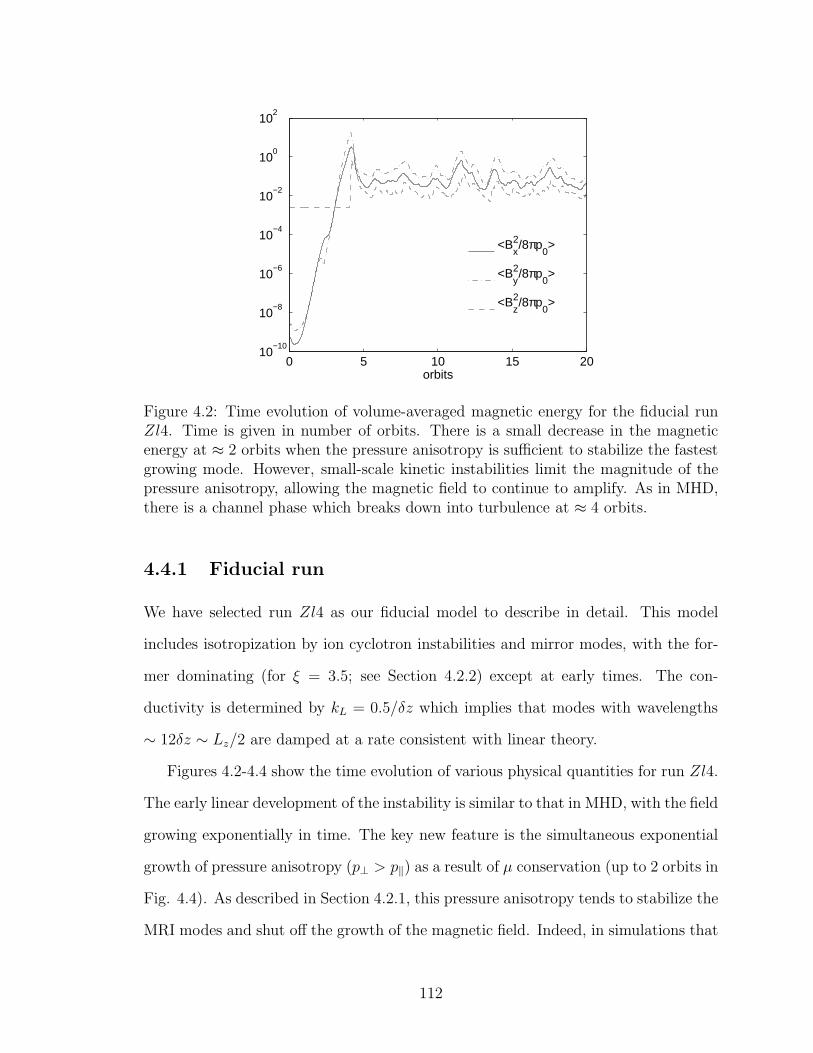
0 5 10 15 2010

−10

10−8

10−6

10−4

10−2

100

102

orbits

<Bx2/8πp

0>

<By2/8πp

0>

<Bz2/8πp

0>

Figure 4.2: Time evolution of volume-averaged magnetic energy for the fiducial runZl4. Time is given in number of orbits. There is a small decrease in the magneticenergy at ≈ 2 orbits when the pressure anisotropy is sufficient to stabilize the fastestgrowing mode. However, small-scale kinetic instabilities limit the magnitude of thepressure anisotropy, allowing the magnetic field to continue to amplify. As in MHD,there is a channel phase which breaks down into turbulence at ≈ 4 orbits.

4.4.1 Fiducial run

We have selected run Zl4 as our fiducial model to describe in detail. This model

includes isotropization by ion cyclotron instabilities and mirror modes, with the for-

mer dominating (for ξ = 3.5; see Section 4.2.2) except at early times. The con-

ductivity is determined by kL = 0.5/δz which implies that modes with wavelengths

∼ 12δz ∼ Lz/2 are damped at a rate consistent with linear theory.

Figures 4.2-4.4 show the time evolution of various physical quantities for run Zl4.

The early linear development of the instability is similar to that in MHD, with the field

growing exponentially in time. The key new feature is the simultaneous exponential

growth of pressure anisotropy (p⊥ > p‖) as a result of µ conservation (up to 2 orbits in

Fig. 4.4). As described in Section 4.2.1, this pressure anisotropy tends to stabilize the

MRI modes and shut off the growth of the magnetic field. Indeed, in simulations that

112

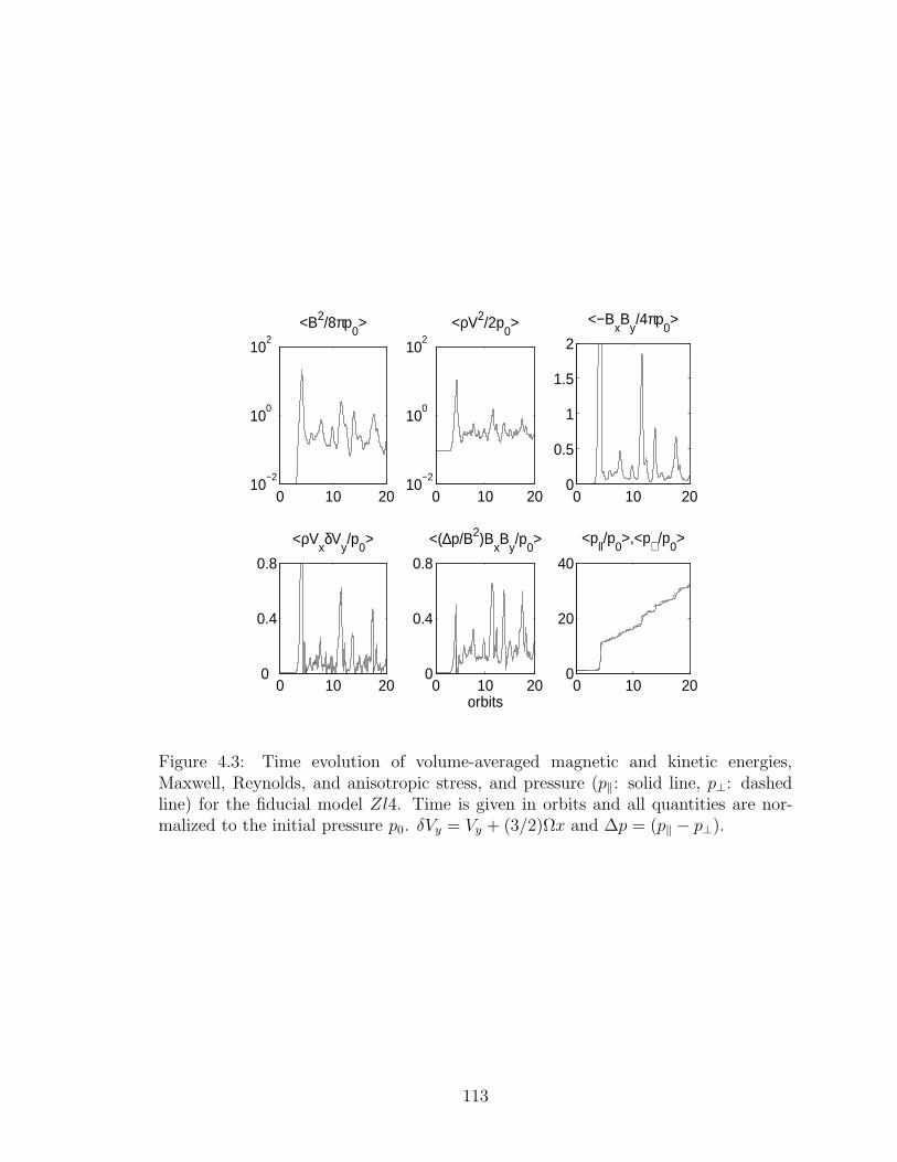
0 10 2010

−2

100

102

<ρV2/2p0>

0 10 200

0.5

1

1.5

2

<−BxB

y/4πp

0>

0 10 200

0.4

0.8

<ρVxδV

y/p

0>

0 10 200

0.4

0.8

<(∆p/B2)BxB

y/p

0>

orbits0 10 20

0

20

40

<pll/p

0>,<p⊥ /p

0>

0 10 2010

−2

100

102

<B2/8πp0>

Figure 4.3: Time evolution of volume-averaged magnetic and kinetic energies,Maxwell, Reynolds, and anisotropic stress, and pressure (p‖: solid line, p⊥: dashedline) for the fiducial model Zl4. Time is given in orbits and all quantities are nor-malized to the initial pressure p0. δVy = Vy + (3/2)Ωx and ∆p = (p‖ − p⊥).

113

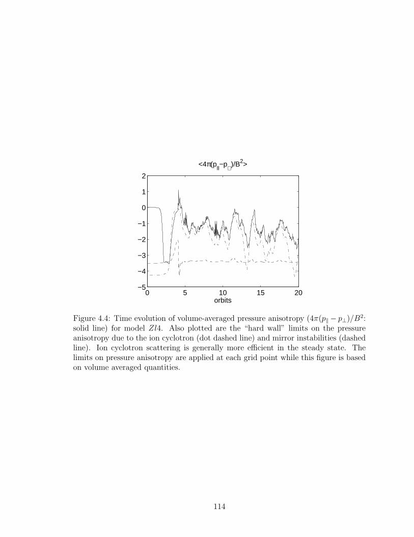
0 5 10 15 20−5

−4

−3

−2

−1

0

1

2

orbits

<4π(pll−p⊥ )/B2>

Figure 4.4: Time evolution of volume-averaged pressure anisotropy (4π(p‖ − p⊥)/B2:solid line) for model Zl4. Also plotted are the “hard wall” limits on the pressureanisotropy due to the ion cyclotron (dot dashed line) and mirror instabilities (dashedline). Ion cyclotron scattering is generally more efficient in the steady state. Thelimits on pressure anisotropy are applied at each grid point while this figure is basedon volume averaged quantities.

114

do not include any isotropization of the pressure tensor, we find that all MRI modes

in the box are stabilized by the pressure anisotropy and the simulation saturates with

the box filled with small amplitude anisotropic Alfven waves (see Figure 4.6). This

highlights the fact that, unlike in MHD, the MRI is not an exact nonlinear solution in

kinetic theory. However, the pressure anisotropy required to stabilize all MRI modes

exceeds the pressure anisotropy at which pitch angle scattering due to mirror and ion

cyclotron instabilities become important. This takes place at about orbit 2 in run

Zl4 (see the small ‘dip’ in the growth of magnetic energies in Figure 4.2), at which

point the pressure anisotropy is significantly reduced and the magnetic field is able

to grow to nonlinear amplitudes.

The nonlinear saturation at orbit ∼ 5 appears qualitatively similar to that in

MHD, and may occur via analogues of the parasitic instabilities described by [75].

The channel solution is, however, much more extreme in KMHD than MHD (the

maximum B2 in Figure 4.2 is approximately an order of magnitude larger than in

analogous MHD runs). After saturation, the magnetic and kinetic energies in the

saturated state are comparable in KMHD and MHD (see Table 4.1). This is essentially

because the pitch angle scattering induced by the kinetic microinstabilities acts to

isotropize the pressure, enforcing a degree of MHD-like dynamics on the collisionless

plasma.

Figure 4.3 and Table 4.1 show the various contributions to the total stress. As

in MHD, the Reynolds stress is significantly smaller than the Maxwell stress. In

kinetic theory, however, there is an additional component to the stress due to the

anisotropic pressure (Eq. 4.48). In the saturated state, we find that the Maxwell stress

is similar in KMHD and MHD, but that the anisotropic stress itself is comparable

to the Maxwell stress. Expressed in terms of an α normalized to the initial pressure,

our fiducial run Zl4 has αM = 0.23, αR = 0.097, and αA = 0.2, indicating that stress

due to pressure anisotropy is dynamically important.

115

Nearly all physical quantities in Figures 4.2-4.4 reach an approximate statistical

steady state. The exceptions are p‖ and p⊥, which increase steadily in time because

the momentum flux on the boundaries does work on the system (Eq. 4.46), which is

eventually converted to heat in the plasma by artificial viscosity; there is no cooling

for internal energy to reach a steady state (the same is true in HGB’s MHD simula-

tions). Because of the steadily increasing internal energy and approximately fixed B2

(although with large fluctuations), the plasma β shows a small secular increase from

orbits 5-20 (a factor of ≈ 3 increase, though with very large fluctuations due to the

large fluctuations in magnetic energy).

Figure 4.4 shows the pressure anisotropy thresholds due to the ion cyclotron and

mirror instabilities, in addition to the volume averaged pressure anisotropy in run Zl4.

From Eq. 4.35, the ion cyclotron threshold (4π∆p/B2) is expected to scale as√

β‖,

which is fairly consistent with the trend in Figure 4.4. The actual pressure anisotropy

in the simulation shows a small increase in time as well, although less than that of the

ion cyclotron threshold. These secular changes in β and ∆p are a consequence of the

increasing internal energy in the shearing box, and are probably not realistic. In a

global disk, we expect that—except perhaps near the inner and outer boundaries—β

will not undergo significant secular changes in time. In a small region of a real disk

in statistical equilibrium, the heating would be balanced by radiation (for thin disks)

or by cooler plasma entering at large R and hotter plasma leaving at small R (in low

luminosity, thick disks).

It is interesting to note that in Figure 4.4, the pressure anisotropy (4π∆p/B2)

is closely tied to the ion cyclotron threshold at times when B2 is rising (which

corresponds to the channel solution reemerging). Increasing B leads to a pressure

anisotropy with p⊥ > p‖ by µ conservation. At the same time, the ion cyclotron

threshold (∼√β) decreases, eventually the pressure limiting threshold is encoun-

tered. When B is decreasing, however, we do not find the same tight relationship

116

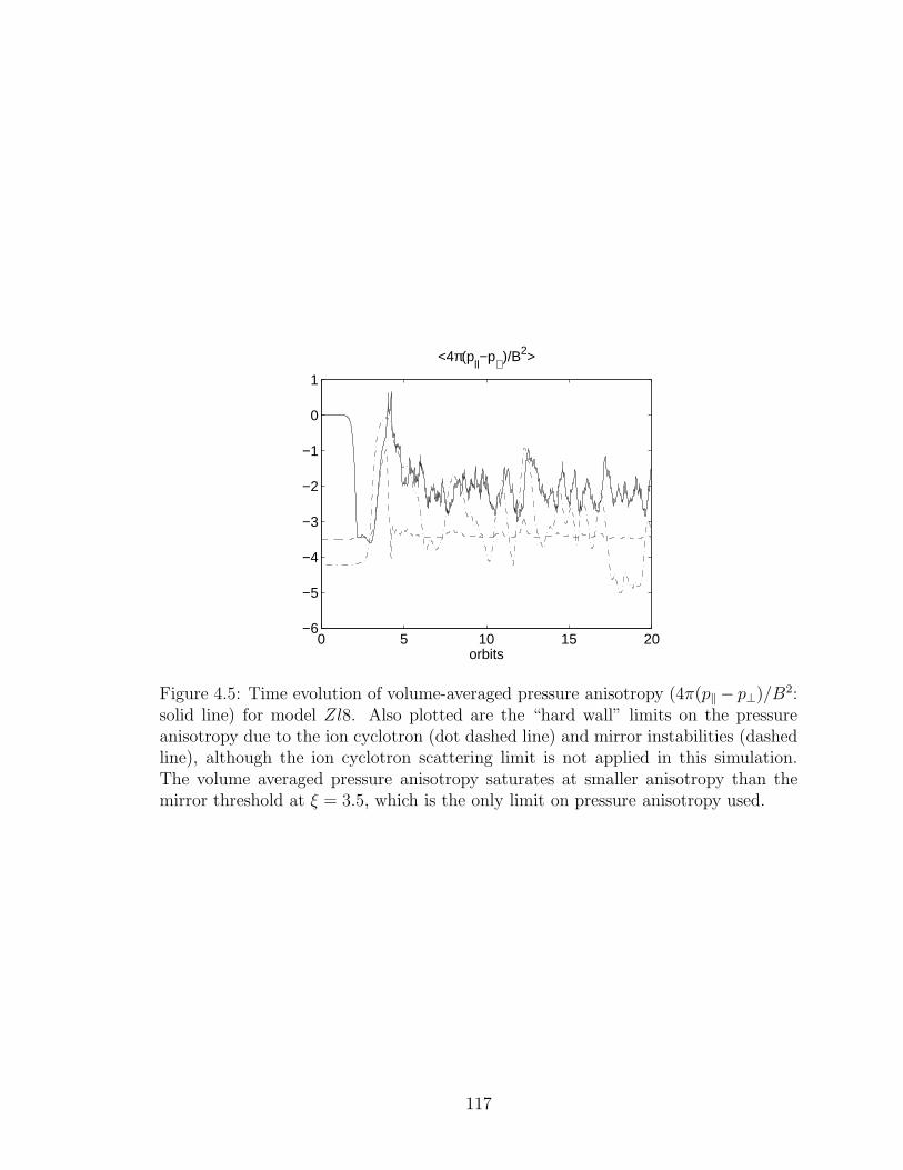
0 5 10 15 20−6

−5

−4

−3

−2

−1

0

1

<4π(pll−p⊥ )/B2>

orbits

Figure 4.5: Time evolution of volume-averaged pressure anisotropy (4π(p‖ − p⊥)/B2:solid line) for model Zl8. Also plotted are the “hard wall” limits on the pressureanisotropy due to the ion cyclotron (dot dashed line) and mirror instabilities (dashedline), although the ion cyclotron scattering limit is not applied in this simulation.The volume averaged pressure anisotropy saturates at smaller anisotropy than themirror threshold at ξ = 3.5, which is the only limit on pressure anisotropy used.

117

between the pressure anisotropy and the imposed threshold. Figure 4.4 clearly indi-

cates that in our fiducial simulation pitch angle scattering is dominated by the ion

cyclotron threshold. For comparison, Figure 4.5 shows the pressure anisotropy and

thresholds for run Zl8 which is identical to the fiducial run, except that the ion cy-

clotron threshold is not used and the only scattering is due to the mirror threshold.

In this case, the saturated pressure anisotropy is somewhat larger than in the fiducial

run, but the pressure anisotropy is not tied to the mirror threshold.

Table 4.2 gives the mean, standard deviation, and standard error in the mean, for

various quantities in the saturated portion of the fiducial simulation. The standard

errors are estimated by taking into account the finite correlation time for the physical

quantities in the simulation, as described in Appendix D. In many cases, the devia-

tions are significantly larger than the mean. As in MHD, we find that the magnetic

energy is dominated by the y- component, which is about a factor of 3 larger than

the x- component; the vertical component is smaller yet. The radial and azimuthal

kinetic energy fluctuations are comparable, while the vertical component is smaller.

We also find that, as in MHD, the perturbed kinetic and magnetic energies are not

in exact equipartition: the magnetic energy is consistently larger. Table 4.2 also

shows the mean and deviations for 〈p⊥/B〉 and 〈p‖B2/ρ2〉. Because of pitch angle

scattering µ = 〈p⊥/B〉 is no longer conserved. 〈p‖B2/ρ2〉 varies because of both, heat

conduction and pitch angle scattering.

The pressure anisotropy in our fiducial run saturates at 4π(p⊥ − p‖)/B2 ≈ 1.5.

By contrast, the threshold for the mirror instability is 4π(p⊥ − p‖)/B2 = 0.5. This

implies that the model is unstable to generating mirror modes. However, the mirror

modes that can be excited at this level of anisotropy do not violate µ conservation

and thus do not contribute to pitch angle scattering (see Section 4.2.2). They can in

principle isotropize the plasma in a volume averaged sense by spatially redistributing

plasma into magnetic wells [101]. This saturation mechanism is simulated using our

118

kinetic MHD code for a uniform, anisotropic plasma (see Appendix C.3.3). It does

not appear to be fully efficient in the saturated state of our turbulent disk simulations,

even at the highest resolution; strong MRI turbulence dominates over everything else

for these parameters.

In the next few sections we compare the fiducial simulation described above with

variations in the pitch angle scattering model and the parallel conductivity. A com-

parison of the total stress in all of our simulations is shown in Figure 4.7.

4.4.2 The double adiabatic limit

Simulations Zl1 and Zh1 are simulations in the double adiabatic limit (no heat

conduction), with no limit on the pressure anisotropy imposed. In this limit both

µ = 〈p⊥/B〉 and 〈p‖B2/ρ2〉 are conserved. Figure 4.6 shows volume averages of

various quantities as a function of time for the run Zl1. These calculations are

very different from the rest of our results and show saturation at very low ampli-

tudes (δB2/B2 ≈ 0.04). In the saturated state, the box is filled with shear modified

anisotropic Alfven waves and all physical quantities are oscillating in time. The total

stress is also oscillatory with a vanishing mean, resulting in negligible transport. In

these calculations, the pressure anisotropy grows to such a large value that it shuts

off the growth of all of the resolved MRI modes in the box. Table 4.1 shows that

〈〈4π(p‖−p⊥)/B2〉〉 saturates at −11.96 and −10.2 for the low and high resolution runs,

respectively (although the normalized pressure anisotropy 〈〈(p‖−p⊥)/p‖〉〉 ≈ −0.07 is

quite small). This is much larger than the anisotropy thresholds for pitch angle scat-

tering described in Subsection 4.2.2. As a result, we do not expect these cases to be

representative of the actual physics of collisionless disks. These cases are of interest,

however, in supporting the predictions of the linear theory with anisotropic initial

conditions considered in Section 4.2.1, and in providing a simple test for the simula-

tions. They also highlight the central role of pressure isotropization in collisionless

119

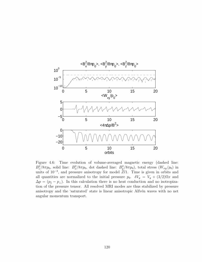
0 5 10 15 2010

−10

10−5

100

<Bx2/8πp

0>, <B

y2/8πp

0>, <B

z2/8πp

0>

0 5 10 15 20−5

0

5

<Wxy

/p0>

0 5 10 15 20

−20

−10

0<4π∆p/B2>

orbits

Figure 4.6: Time evolution of volume-averaged magnetic energy (dashed line:B2

z/8πp0, solid line: B2x/8πp0, dot dashed line: B2

y/8πp0), total stress (Wxy/p0) inunits of 10−3, and pressure anisotropy for model Zl1. Time is given in orbits andall quantities are normalized to the initial pressure p0. δVy = Vy + (3/2)Ωx and∆p = (p‖ − p⊥). In this calculation there is no heat conduction and no isotropiza-tion of the pressure tensor. All resolved MRI modes are thus stabilized by pressureanisotropy and the ‘saturated’ state is linear anisotropic Alfven waves with no netangular momentum transport.

120

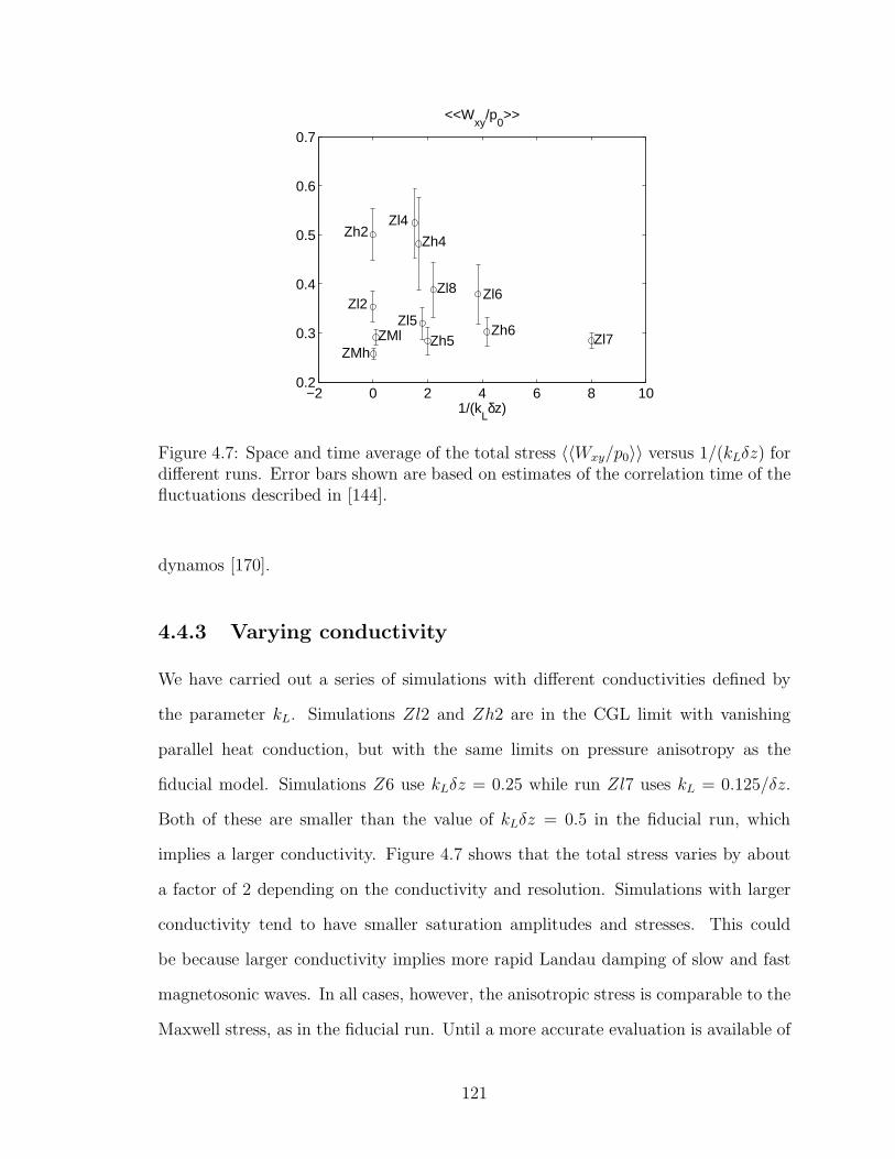
−2 0 2 4 6 8 100.2

0.3

0.4

0.5

0.6

0.7

<<Wxy

/p0>>

1/(kLδz)

Zh2

Zl2

ZMlZMh

Zl4

Zh4

Zl8

Zl5

Zh5

Zl6

Zh6Zl7

Figure 4.7: Space and time average of the total stress 〈〈Wxy/p0〉〉 versus 1/(kLδz) fordifferent runs. Error bars shown are based on estimates of the correlation time of thefluctuations described in [144].

dynamos [170].

4.4.3 Varying conductivity

We have carried out a series of simulations with different conductivities defined by

the parameter kL. Simulations Zl2 and Zh2 are in the CGL limit with vanishing

parallel heat conduction, but with the same limits on pressure anisotropy as the

fiducial model. Simulations Z6 use kLδz = 0.25 while run Zl7 uses kL = 0.125/δz.

Both of these are smaller than the value of kLδz = 0.5 in the fiducial run, which

implies a larger conductivity. Figure 4.7 shows that the total stress varies by about

a factor of 2 depending on the conductivity and resolution. Simulations with larger

conductivity tend to have smaller saturation amplitudes and stresses. This could

be because larger conductivity implies more rapid Landau damping of slow and fast

magnetosonic waves. In all cases, however, the anisotropic stress is comparable to the

Maxwell stress, as in the fiducial run. Until a more accurate evaluation is available of

121

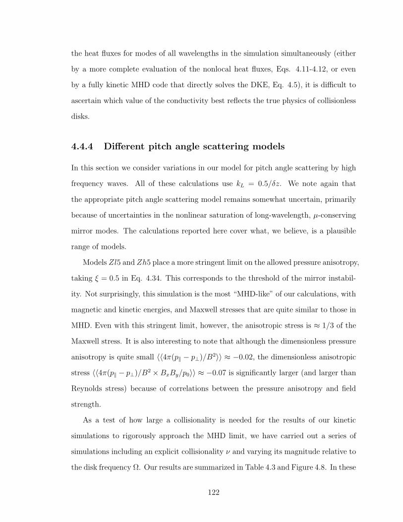
the heat fluxes for modes of all wavelengths in the simulation simultaneously (either

by a more complete evaluation of the nonlocal heat fluxes, Eqs. 4.11-4.12, or even

by a fully kinetic MHD code that directly solves the DKE, Eq. 4.5), it is difficult to

ascertain which value of the conductivity best reflects the true physics of collisionless

disks.

4.4.4 Different pitch angle scattering models

In this section we consider variations in our model for pitch angle scattering by high

frequency waves. All of these calculations use kL = 0.5/δz. We note again that

the appropriate pitch angle scattering model remains somewhat uncertain, primarily

because of uncertainties in the nonlinear saturation of long-wavelength, µ-conserving

mirror modes. The calculations reported here cover what, we believe, is a plausible

range of models.

Models Zl5 and Zh5 place a more stringent limit on the allowed pressure anisotropy,

taking ξ = 0.5 in Eq. 4.34. This corresponds to the threshold of the mirror instabil-

ity. Not surprisingly, this simulation is the most “MHD-like” of our calculations, with

magnetic and kinetic energies, and Maxwell stresses that are quite similar to those in

MHD. Even with this stringent limit, however, the anisotropic stress is ≈ 1/3 of the

Maxwell stress. It is also interesting to note that although the dimensionless pressure

anisotropy is quite small 〈〈4π(p‖ − p⊥)/B2〉〉 ≈ −0.02, the dimensionless anisotropic

stress 〈〈4π(p‖ − p⊥)/B2 ×BxBy/p0〉〉 ≈ −0.07 is significantly larger (and larger than

Reynolds stress) because of correlations between the pressure anisotropy and field

strength.

As a test of how large a collisionality is needed for the results of our kinetic

simulations to rigorously approach the MHD limit, we have carried out a series of

simulations including an explicit collisionality ν and varying its magnitude relative to

the disk frequency Ω. Our results are summarized in Table 4.3 and Figure 4.8. In these

122

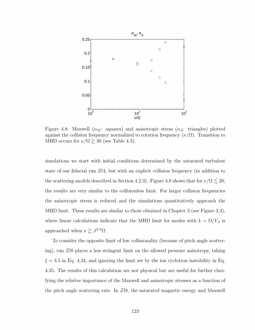
100

101

102

0

0.05

0.1

0.15

0.2

0.25

ν/Ω

αM

, αA

Figure 4.8: Maxwell (αM : squares) and anisotropic stress (αA: triangles) plottedagainst the collision frequency normalized to rotation frequency (ν/Ω). Transition toMHD occurs for ν/Ω & 30 (see Table 4.3).

simulations we start with initial conditions determined by the saturated turbulent

state of our fiducial run Zl4, but with an explicit collision frequency (in addition to

the scattering models described in Section 4.2.3). Figure 4.8 shows that for ν/Ω . 20,

the results are very similar to the collisionless limit. For larger collision frequencies

the anisotropic stress is reduced and the simulations quantitatively approach the

MHD limit. These results are similar to those obtained in Chapter 3 (see Figure 3.3),

where linear calculations indicate that the MHD limit for modes with k ∼ Ω/VA is

approached when ν & β3/4Ω.

To consider the opposite limit of low collisionality (because of pitch angle scatter-

ing), run Zl8 places a less stringent limit on the allowed pressure anisotropy, taking

ξ = 3.5 in Eq. 4.34, and ignoring the limit set by the ion cyclotron instability in Eq.

4.35. The results of this calculation are not physical but are useful for further clari-

fying the relative importance of the Maxwell and anisotropic stresses as a function of

the pitch angle scattering rate. In Zl8, the saturated magnetic energy and Maxwell

123

stress are lower than in all of our other calculations (excluding the double adiabatic

models described in Section 4.4.2). Interestingly, however, the total stress is compa-

rable to that in the other calculations (Figure 4.7) because the anisotropic stress is

≈ 2.4 times larger than the Maxwell stress (Table 4.1). As discussed briefly in Sec-

tion 4.4.1, the pressure anisotropy in this simulation is not simply set by the applied

mirror pitch angle scattering threshold (its quite smaller than the mirror “hard wall;”

see Figure 4.5). It is possible that resolved mirror modes contribute to decreasing the

volume averaged pressure anisotropy (but see below).

Finally, in models Z3 we include parallel heat conduction but do not limit the

pressure anisotropy. In these calculations, we expect to be able to resolve the long-

wavelength µ-conserving mirror modes that reduce the pressure anisotropy by forming

magnetic wells [101].4 In our test problems with uniform anisotropic plasmas, this

is precisely what we find (see Appendix C.3.3). In the shearing box calculations,

however, even at the highest resolutions, we find that the pressure anisotropy becomes

so large that Eqs. 4.34) and 4.35 are violated, so that pitch angle scattering due

to high frequency microinstabilities would become important. The resolved mirror

modes are thus not able to isotropize the pressure sufficiently fast at all places in

the box.5 However, it is hard to draw any firm conclusions from these simulations

because they stop at around 4 orbits (for both resolutions Zl3 and Zh3) during the

initial nonlinear transient stage. At this time the pressure becomes highly anisotropic

and becomes very small at some grid points, and the time step limit causes δt→ 0.

Pitch angle scattering centers are not uniformly distributed in space and show

intermittency. Subsection 2.6.1 gives simple estimates for effective collision frequency

and mean free path assuming a uniform distribution of scattering centers. Also dis-

4At the resolution of Zl3, the fastest growing mirror mode in the computational domain has alinear growth comparable to that of the MRI.

5In higher resolution simulations, one can resolve smaller-scale and faster growing mirror modes,and thus the effects of isotropization by resolved mirror modes could become increasingly important.We see no such indications, however, for the range of resolutions we have been able to simulate.

124

cussed are simulation results which show that only a very small fraction of the box un-

dergoes pitch angle scattering (see Figure 2.2). Figure 2.2 also shows that pitch angle

scattering due to mirror instability dominates ion-cyclotron instability for β & 100.

Intermittency of pitch angle scattering can be crucial for thermal conduction and

viscous transport in collisionless high-β plasmas.

4.5 Additional simulations

Our paper, [177], describes simulations with an initial β = 400 and an initial vertical

field (Bφ = 0). The linear theory predicts that the fastest growing mode for Bφ = Bz

in the kinetic regime is ≈ twice faster than MHD, and at a much larger scale. The scale

separation between the fastest growing kinetic MHD and MHD modes for Bφ = Bz is

greatest for large β (see [158]). In this section we describe simulations not described

in [177]—initial conditions with Bφ = Bz and only Bφ, and the high β regime. One

of the motivations is to see whether a faster growth rate for Bφ = Bz in the kinetic

regime results in a nonlinear saturation different from MHD. The fastest growing

MRI mode in MHD occurs at a scale H/√β, much smaller than the disk height scale

H = cs/Ω for large initial β. Thus, we vary the box size and resolution to study the

effect of these parameters on nonlinear saturation.

4.5.1 High β simulations

Figure 4.9 shows the growth rate of the MRI in the kinetic and MHD regimes for

β = 106—the fastest growing kinetic MRI is at a much larger length scale. Because

of a large separation of scales between the fastest growing modes in the kinetic and

MHD regimes, it is difficult to resolve both the scales in a numerical simulation. The

figure also marks, by arrows, the minimum and maximum wavenumber corresponding

to the chosen box size for the low resolution runs (KY Zl and MY Zl); for these

125

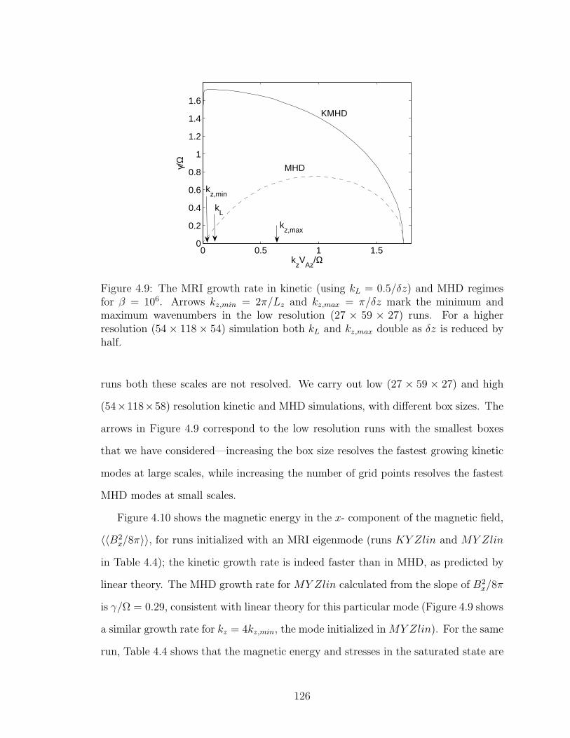
0 0.5 1 1.50

0.2

0.4

0.6

0.8

1

1.2

1.4

1.6

kzV

Az/Ω

γ/Ω

KMHD

MHD

kz,max

kz,min

kL

Figure 4.9: The MRI growth rate in kinetic (using kL = 0.5/δz) and MHD regimesfor β = 106. Arrows kz,min = 2π/Lz and kz,max = π/δz mark the minimum andmaximum wavenumbers in the low resolution (27 × 59 × 27) runs. For a higherresolution (54 × 118 × 54) simulation both kL and kz,max double as δz is reduced byhalf.

runs both these scales are not resolved. We carry out low (27 × 59 × 27) and high

(54×118×58) resolution kinetic and MHD simulations, with different box sizes. The

arrows in Figure 4.9 correspond to the low resolution runs with the smallest boxes

that we have considered—increasing the box size resolves the fastest growing kinetic

modes at large scales, while increasing the number of grid points resolves the fastest

MHD modes at small scales.

Figure 4.10 shows the magnetic energy in the x- component of the magnetic field,

〈〈B2x/8π〉〉, for runs initialized with an MRI eigenmode (runs KY Zlin and MY Zlin

in Table 4.4); the kinetic growth rate is indeed faster than in MHD, as predicted by

linear theory. The MHD growth rate for MY Zlin calculated from the slope of B2x/8π

is γ/Ω = 0.29, consistent with linear theory for this particular mode (Figure 4.9 shows

a similar growth rate for kz = 4kz,min, the mode initialized in MY Zlin). For the same

run, Table 4.4 shows that the magnetic energy and stresses in the saturated state are

126

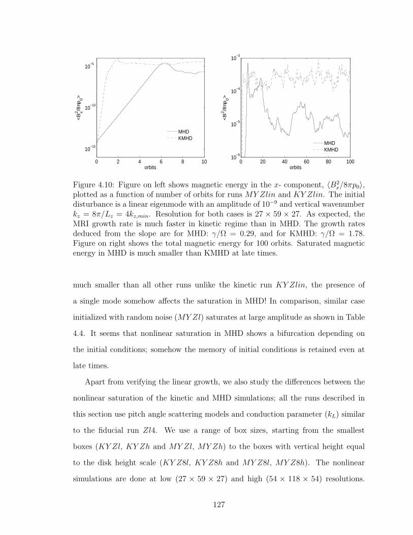
0 2 4 6 8 10

10−15

10−10

10−5

orbits

<B

x2/8

πp0>

MHDKMHD

0 20 40 60 80 10010

−6

10−5

10−4

10−3

orbits

<B

2/8

πp0>

MHDKMHD

Figure 4.10: Figure on left shows magnetic energy in the x- component, 〈B2x/8πp0〉,

plotted as a function of number of orbits for runs MY Zlin and KY Zlin. The initialdisturbance is a linear eigenmode with an amplitude of 10−9 and vertical wavenumberkz = 8π/Lz = 4kz,min. Resolution for both cases is 27 × 59 × 27. As expected, theMRI growth rate is much faster in kinetic regime than in MHD. The growth ratesdeduced from the slope are for MHD: γ/Ω = 0.29, and for KMHD: γ/Ω = 1.78.Figure on right shows the total magnetic energy for 100 orbits. Saturated magneticenergy in MHD is much smaller than KMHD at late times.

much smaller than all other runs unlike the kinetic run KY Zlin, the presence of

a single mode somehow affects the saturation in MHD! In comparison, similar case

initialized with random noise (MY Zl) saturates at large amplitude as shown in Table

4.4. It seems that nonlinear saturation in MHD shows a bifurcation depending on

the initial conditions; somehow the memory of initial conditions is retained even at

late times.

Apart from verifying the linear growth, we also study the differences between the

nonlinear saturation of the kinetic and MHD simulations; all the runs described in

this section use pitch angle scattering models and conduction parameter (kL) similar

to the fiducial run Zl4. We use a range of box sizes, starting from the smallest

boxes (KY Zl, KY Zh and MY Zl, MY Zh) to the boxes with vertical height equal

to the disk height scale (KY Z8l, KY Z8h and MY Z8l, MY Z8h). The nonlinear

simulations are done at low (27 × 59 × 27) and high (54 × 118 × 54) resolutions.

127

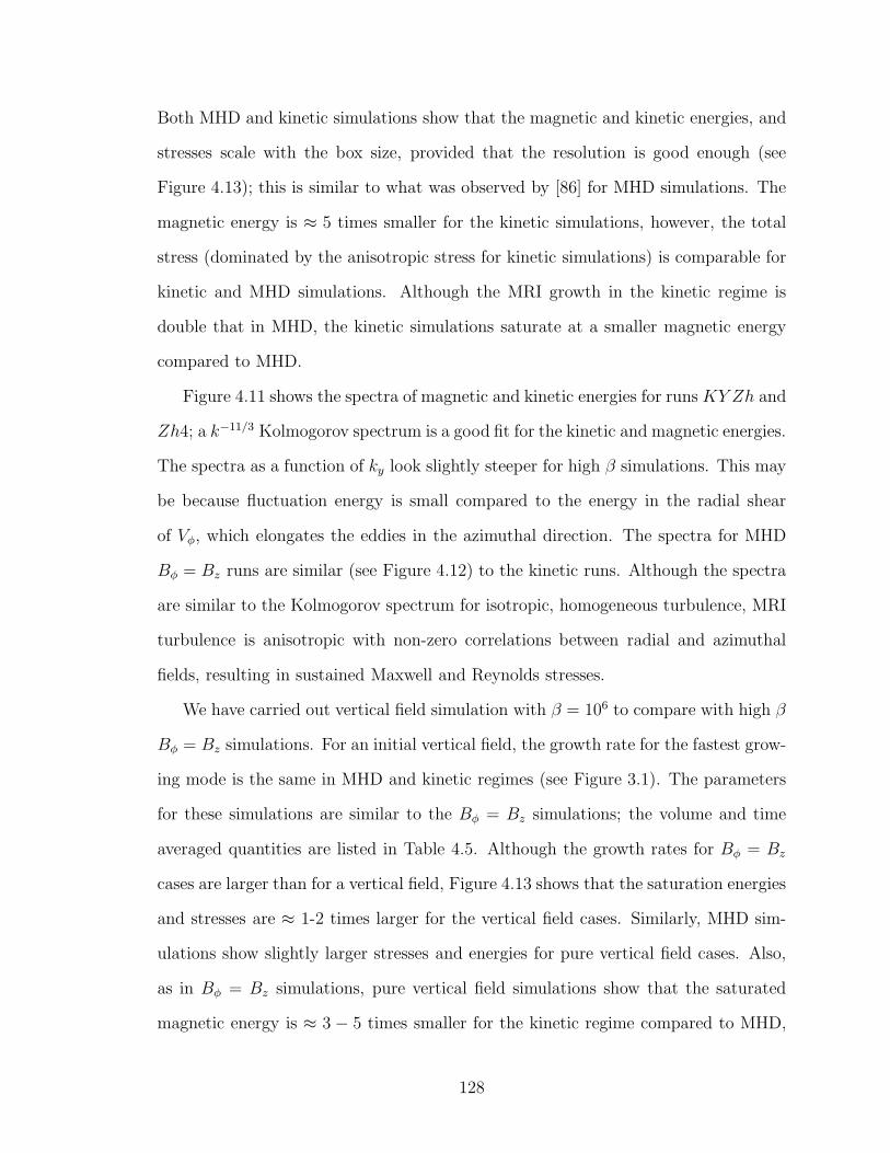
Both MHD and kinetic simulations show that the magnetic and kinetic energies, and

stresses scale with the box size, provided that the resolution is good enough (see

Figure 4.13); this is similar to what was observed by [86] for MHD simulations. The

magnetic energy is ≈ 5 times smaller for the kinetic simulations, however, the total

stress (dominated by the anisotropic stress for kinetic simulations) is comparable for

kinetic and MHD simulations. Although the MRI growth in the kinetic regime is

double that in MHD, the kinetic simulations saturate at a smaller magnetic energy

compared to MHD.

Figure 4.11 shows the spectra of magnetic and kinetic energies for runs KY Zh and

Zh4; a k−11/3 Kolmogorov spectrum is a good fit for the kinetic and magnetic energies.

The spectra as a function of ky look slightly steeper for high β simulations. This may

be because fluctuation energy is small compared to the energy in the radial shear

of Vφ, which elongates the eddies in the azimuthal direction. The spectra for MHD

Bφ = Bz runs are similar (see Figure 4.12) to the kinetic runs. Although the spectra

are similar to the Kolmogorov spectrum for isotropic, homogeneous turbulence, MRI

turbulence is anisotropic with non-zero correlations between radial and azimuthal

fields, resulting in sustained Maxwell and Reynolds stresses.

We have carried out vertical field simulation with β = 106 to compare with high β

Bφ = Bz simulations. For an initial vertical field, the growth rate for the fastest grow-

ing mode is the same in MHD and kinetic regimes (see Figure 3.1). The parameters

for these simulations are similar to the Bφ = Bz simulations; the volume and time

averaged quantities are listed in Table 4.5. Although the growth rates for Bφ = Bz

cases are larger than for a vertical field, Figure 4.13 shows that the saturation energies

and stresses are ≈ 1-2 times larger for the vertical field cases. Similarly, MHD sim-

ulations show slightly larger stresses and energies for pure vertical field cases. Also,

as in Bφ = Bz simulations, pure vertical field simulations show that the saturated

magnetic energy is ≈ 3 − 5 times smaller for the kinetic regime compared to MHD,

128

100

101

102

103

104

10−7

10−6

10−5

10−4

10−3

kVs/Ω

|B(k

)|2/8

πp0

k−11/3

100

101

102

103

104

10−7

10−6

10−5

10−4

10−3

10−2

kVs/Ω

ρ 0|v

(k)|

2/2

p0

k−11/3

100

101

102

103

10−5

10−4

10−3

10−2

10−1

100

kVs/Ω

|B(k

)|2/8

πp0

k−11/3

100

101

102

103

10−5

10−4

10−3

10−2

10−1

100

kVs/Ω

ρ 0|v

(k)|

2/2

p0

k−11/3

Figure 4.11: Turbulent magnetic (|B(k)|2/8πp0) and kinetic energy (ρ0|V (k)|2/2p0)spectra for kinetic MHD: the β = 106 run KY Zh (top), and the β = 400 initialvertical field case (bottom, run Zh4 in [177]; see Table 4.1). Spectra with respectto kx (solid line), ky (dashed line) and kz (dotted line) are shown. Also shown isthe k−11/3 Kolmogorov spectrum. The magnetic and kinetic energies for KY Zh aremuch smaller than for Zh4. For top figures, spectra with respect to ky are steeper,because for β = 106 cases shear in velocity Vy dominates the fluctuations, causing theeddies to be elongated in the y- direction, with a steeper spectrum. The spectra areaveraged in the other two directions in k- space; e.g., for a spectrum with respect tokx, |B|2(kx) =

∫

dkydkzB(kx, ky, kz)B∗(kx, ky, kz).

129

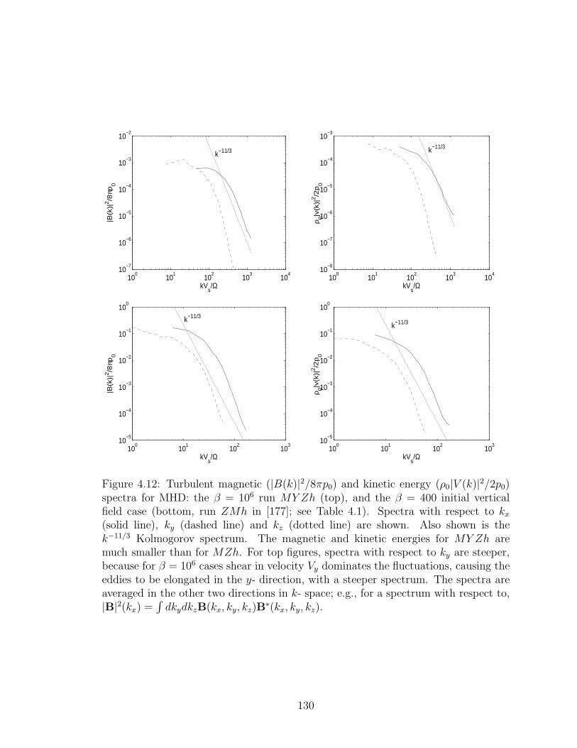
100

101

102

103

104

10−7

10−6

10−5

10−4

10−3

10−2

kVs/Ω

|B(k

)|2/8

πp0

k−11/3

100

101

102

103

104

10−8

10−7

10−6

10−5

10−4

10−3

kVs/Ω

ρ 0|v

(k)|

2/2

p0

k−11/3

100

101

102

103

10−5

10−4

10−3

10−2

10−1

100

kVs/Ω

|B(k

)|2/8

πp0

k−11/3

100

101

102

103

10−5

10−4

10−3

10−2

10−1

100

kVs/Ω

ρ 0|v

(k)|

2/2

p0k−11/3

Figure 4.12: Turbulent magnetic (|B(k)|2/8πp0) and kinetic energy (ρ0|V (k)|2/2p0)spectra for MHD: the β = 106 run MY Zh (top), and the β = 400 initial verticalfield case (bottom, run ZMh in [177]; see Table 4.1). Spectra with respect to kx

(solid line), ky (dashed line) and kz (dotted line) are shown. Also shown is thek−11/3 Kolmogorov spectrum. The magnetic and kinetic energies for MY Zh aremuch smaller than for MZh. For top figures, spectra with respect to ky are steeper,because for β = 106 cases shear in velocity Vy dominates the fluctuations, causing theeddies to be elongated in the y- direction, with a steeper spectrum. The spectra areaveraged in the other two directions in k- space; e.g., for a spectrum with respect to,|B|2(kx) =

∫

dkydkzB(kx, ky, kz)B∗(kx, ky, kz).

130

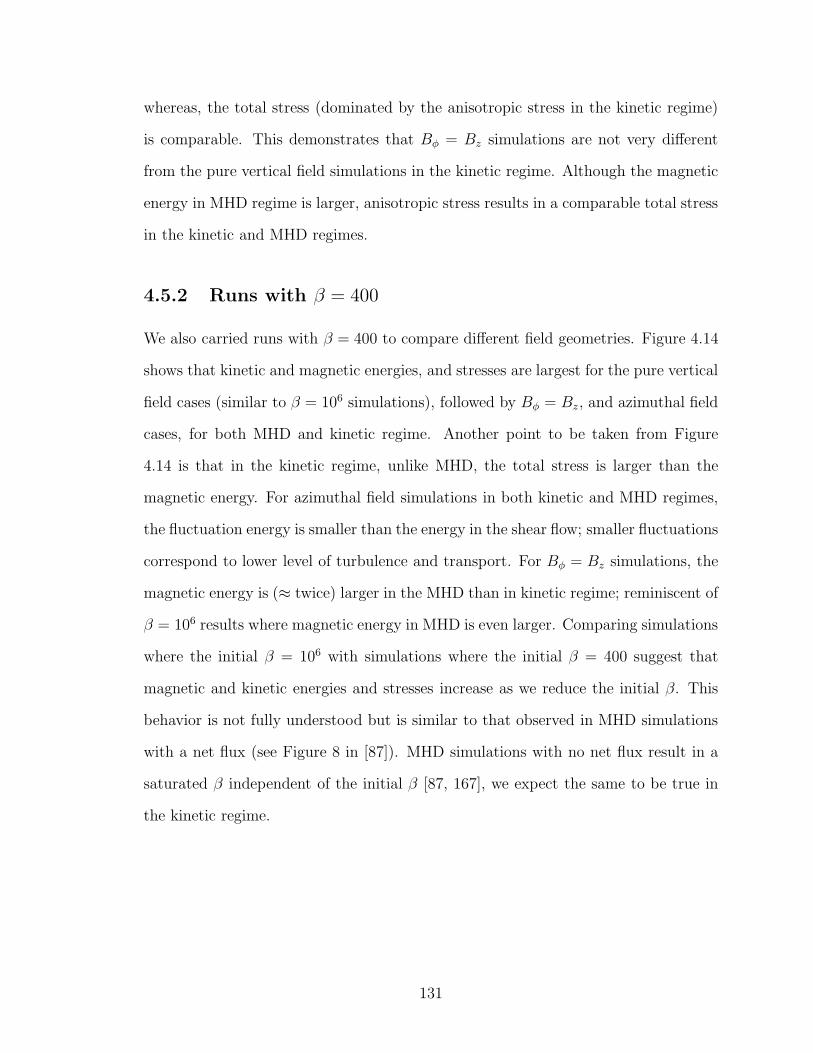
whereas, the total stress (dominated by the anisotropic stress in the kinetic regime)

is comparable. This demonstrates that Bφ = Bz simulations are not very different

from the pure vertical field simulations in the kinetic regime. Although the magnetic

energy in MHD regime is larger, anisotropic stress results in a comparable total stress

in the kinetic and MHD regimes.

4.5.2 Runs with β = 400

We also carried runs with β = 400 to compare different field geometries. Figure 4.14

shows that kinetic and magnetic energies, and stresses are largest for the pure vertical

field cases (similar to β = 106 simulations), followed by Bφ = Bz, and azimuthal field

cases, for both MHD and kinetic regime. Another point to be taken from Figure

4.14 is that in the kinetic regime, unlike MHD, the total stress is larger than the

magnetic energy. For azimuthal field simulations in both kinetic and MHD regimes,

the fluctuation energy is smaller than the energy in the shear flow; smaller fluctuations

correspond to lower level of turbulence and transport. For Bφ = Bz simulations, the

magnetic energy is (≈ twice) larger in the MHD than in kinetic regime; reminiscent of

β = 106 results where magnetic energy in MHD is even larger. Comparing simulations

where the initial β = 106 with simulations where the initial β = 400 suggest that

magnetic and kinetic energies and stresses increase as we reduce the initial β. This

behavior is not fully understood but is similar to that observed in MHD simulations

with a net flux (see Figure 8 in [87]). MHD simulations with no net flux result in a

saturated β independent of the initial β [87, 167], we expect the same to be true in

the kinetic regime.

131

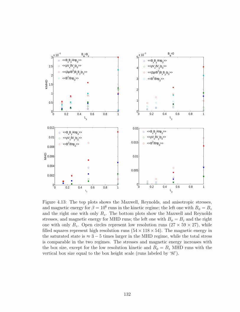
0 0.2 0.4 0.6 0.8 10

0.5

1

1.5

2

2.5

3x 10

−3

Lz

KM

HD

Bφ=Bz

<<B

xB

y/4πp

0>>

<<ρVxδV

y/p

0>>

<<(∆p/B2)BxB

y/p

0>>

<<B2/8πp0>>

0 0.2 0.4 0.6 0.8 10

1

2

3

4

5x 10

−3

Lz

Bφ=0

<<BxB

y/4πp

0>>

<<ρVxδV

y/p

0>>

<<(∆p/B2)BxB

y/p

0>>

<<B2/8πp0>>

0 0.2 0.4 0.6 0.8 10

0.002

0.004

0.006

0.008

0.01

0.012

Lz

MH

D

<<BxB

y/4πp

0>>

<<ρVxδV

y/p

0>>

<<B2/8πp0>>

0 0.2 0.4 0.6 0.8 10

0.005

0.01

0.015

0.02

Lz

<<BxB

y/4πp

0>>

<<ρVxδV

y/p

0>>

<<B2/8πp0>>

Figure 4.13: The top plots shows the Maxwell, Reynolds, and anisotropic stresses,and magnetic energy for β = 106 runs in the kinetic regime; the left one with Bφ = Bz

and the right one with only Bz. The bottom plots show the Maxwell and Reynoldsstresses, and magnetic energy for MHD runs; the left one with Bφ = Bz and the rightone with only Bz. Open circles represent low resolution runs (27 × 59 × 27), whilefilled squares represent high resolution runs (54× 118× 54). The magnetic energy inthe saturated state is ≈ 3− 5 times larger in the MHD regime, while the total stressis comparable in the two regimes. The stresses and magnetic energy increases withthe box size, except for the low resolution kinetic and Bφ = Bz MHD runs with thevertical box size equal to the box height scale (runs labeled by ‘8l’).

132

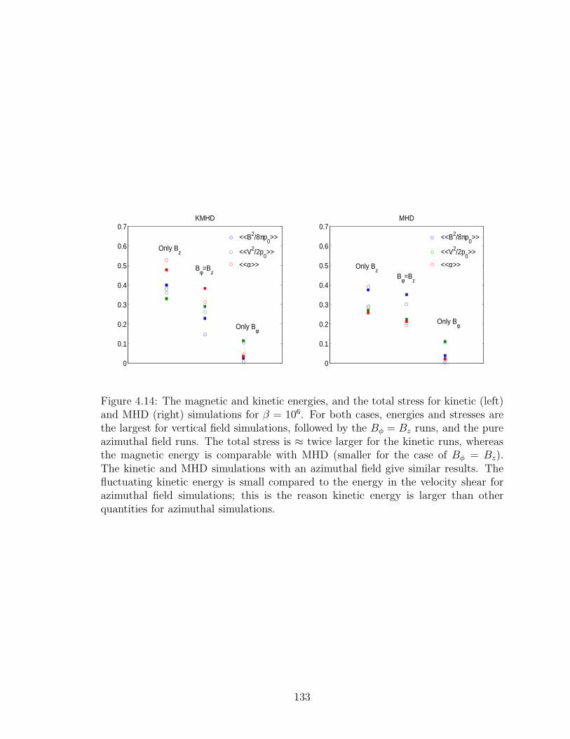
0

0.1

0.2

0.3

0.4

0.5

0.6

0.7KMHD

<<B2/8πp0>>

<<V2/2p0>>

<<α>>

Only Bz

Bφ=Bz

Only Bφ

0

0.1

0.2

0.3

0.4

0.5

0.6

0.7MHD

<<B2/8πp0>>

<<V2/2p0>>

<<α>>Only Bz

Bφ=Bz

Only Bφ

Figure 4.14: The magnetic and kinetic energies, and the total stress for kinetic (left)and MHD (right) simulations for β = 106. For both cases, energies and stresses arethe largest for vertical field simulations, followed by the Bφ = Bz runs, and the pureazimuthal field runs. The total stress is ≈ twice larger for the kinetic runs, whereasthe magnetic energy is comparable with MHD (smaller for the case of Bφ = Bz).The kinetic and MHD simulations with an azimuthal field give similar results. Thefluctuating kinetic energy is small compared to the energy in the velocity shear forazimuthal field simulations; this is the reason kinetic energy is larger than otherquantities for azimuthal simulations.

133

4.6 Summary and Discussion

In this chapter we have described our local shearing box simulations of the mag-

netorotational instability in a collisionless plasma [177]. We are motivated by the

application to hot radiatively inefficient flows which are believed to be present in

many low-luminosity accreting systems (see Section 1.4). Our method for simulating

the dynamics of a collisionless plasma is fluid-based, and relies on evolving a pressure

tensor with closure models for the heat flux along magnetic field lines. These heat

flux models can be thought of as approximating the collisionless (Landau) damping

of linear modes in the simulation.

By adiabatic invariance, a slow increase (decrease) in the magnetic field strength

tends to give rise to a pressure anisotropy with p⊥ > p‖ (p‖ > p⊥), where the sign of

anisotropy is defined by the local magnetic field. Such a pressure anisotropy can, how-

ever, give rise to small scale kinetic instabilities (firehose, mirror, and ion cyclotron)

which act to isotropize the pressure tensor, effectively providing an enhanced rate of

pitch angle scattering (“collisions”). We have included the effects of this isotropization

via a subgrid model which restricts the allowed magnitude of the pressure anisotropy

(see Section 4.2.3).

We find that the nonlinear evolution of the MRI in a collisionless plasma is quali-

tatively similar to that in MHD, with comparable saturation magnetic field strengths

and magnetic stresses. The primary new effect in kinetic theory is the existence of

angular momentum transport due to the anisotropic pressure stress (Eq. 4.48). For

the allowed pressure anisotropies estimated in Section 4.2.3, the anisotropic stress is

dynamically important and is as large as the Maxwell stress (Table 4.1). The high

β Bφ = Bz simulations, although showing the expected faster growth rate than in

MHD, show a smaller magnetic energy (factor of ∼ 5) in the kinetic regime, but the

total stress is comparable to MHD. Although the MRI in kinetic and MHD regimes

is different linearly (with the fastest growing mode in the kinetic regime twice faster

134

than in MHD), they are qualitatively similar in the nonlinear regime.

The precise rate of transport in the present simulations is difficult to quantify

accurately and depends—at the factor of ∼ 2 level—on some of the uncertain micro-

physics in our kinetic analysis (e.g., the rate of heat conduction along magnetic field

lines and the exact threshold for pitch angle scattering by small-scale instabilities; see

Figure 4.7). For better results, it would be interesting to extend these calculations

with a more accurate evaluation of the actual nonlocal heat fluxes, Eqs. 4.11-4.12, or

even to directly solve the drift kinetic equation, Eq. 4.5, for the particle distribution

function. Further kinetic studies in the local shearing box, including studies of the

small-scale instabilities that limit pressure anisotropy, would be helpful in developing

appropriate fluid closures for global simulations.

It is interesting to note that two-temperature RIAFs can only be maintained below

a critical luminosity ∼ α2LEDD [163]. Thus enhanced transport in kinetic theory due

to the anisotropic pressure stress would extend upward in luminosity the range of

systems to which RIAFs could be applicable. This is important for understanding,

e.g., state transitions in X-ray binaries [55].

In addition to angular momentum transport by anisotropic pressure stresses, Lan-

dau damping of long-wavelength modes can be important in heating collisionless ac-

cretion flows. Because the version of ZEUS MHD code we use is non-conservative,

we cannot carry out a rigorous calculation of heating by different mechanisms such

as Landau damping and reconnection. Following the total energy-conserving scheme

of [194], however, we estimate that the energy dissipated by collisionless damping

(present in the form of work done by anisotropic stress) is comparable to or larger

than that due to numerical magnetic energy loss (which is the major source of heating

in MHD simulations), which represents both energy lost due to reconnection and the

energy cascading beyond the scales at the resolution limit. One caveat to studying

energetics in a local shearing box is that in local simulations, the pressure increases

135

in time due to heating, while B2 ∼ constant. Thus β increases in time and the tur-

bulence becomes more and more incompressible. This will artificially decrease the

importance of compressible channels of heating. Clearly it is of significant interest

to better understand heating and energy dissipation in RIAFs, particularly for the

electrons. The one fluid simulations provide some indications of electron heating in

RIAFs; electrons will also be anisotropic because of magnetic energy fluctuations.

The pressure anisotropy in electrons is also limited due to microinstabilities, e.g., the

electron whistler instability considered by [68]. The heating rate of electrons due to

anisotropic stress (d ln p/dt) is comparable to that of ions because pressure anisotropy

is comparable for electrons and ions. For RIAFs, it may mean that electrons cannot

be kept too cool compared to the ion; but systematic 2-fluid simulations that account

for all sources of heating are needed to draw firm conclusions.

In all of our calculations, we have assumed that the dominant source of pitch

angle scattering is high frequency microinstabilities generated during the growth and

nonlinear evolution of the MRI. We cannot, however, rule out that there are other

sources of high frequency waves that pitch angle scatter and effectively decrease the

mean free path of particles relative to that calculated here (e.g., shocks and recon-

nection). As shown in Table 4.3 and Figure 4.8, this would decrease the magnitude of

the anisotropic stress; we find that for ν & 30 Ω, the results of our kinetic simulations

quantitatively approach the MHD limit. In this context it is important to note that

the incompressible part of the MHD cascade launched by the MRI is expected to be

highly anisotropic with k⊥ ≫ k‖ [73]. As a result, there is very little power in high

frequency waves that could break µ conservation. It is also interesting to note that

satellites have observed that the pressure anisotropy in the solar wind near 1 AU is

approximately marginally stable to the firehose instability [98], consistent with our

assumption that microinstabilities dominate the isotropization of the plasma. There

is evidence for pressure anisotropy in other collisionless plasmas, e.g., the solar wind

136

[123, 98] and magnetosphere [192, 66].

In this chapter we have focused on kinetic modifications to angular momentum

transport via anisotropic pressure stresses and parallel heat conduction. In addition,

kinetic effects substantially modify the stability of thermally stratified low collisional-

ity plasmas such as those expected in RIAFs. Balbus [10] showed that in the presence

of anisotropic heat conduction, thermally stratified plasmas are unstable when the

temperature decreases outwards, rather than when the entropy decreases outwards

(the usual Schwarzschild criterion). This has been called the magnetothermal instabil-

ity (MTI). Parrish and Stone [148] show that in non-rotating atmospheres the MTI

leads to magnetic field amplification and efficient heat transport. In future global

simulations of RIAFs, it will be interesting to explore the combined dynamics of the

MTI, the MRI, and angular momentum transport via anisotropic pressure stresses.

Apart from affecting the local dynamics and energetics, collisionless effects can affect

the global structure of hot, collisionless disks.

137

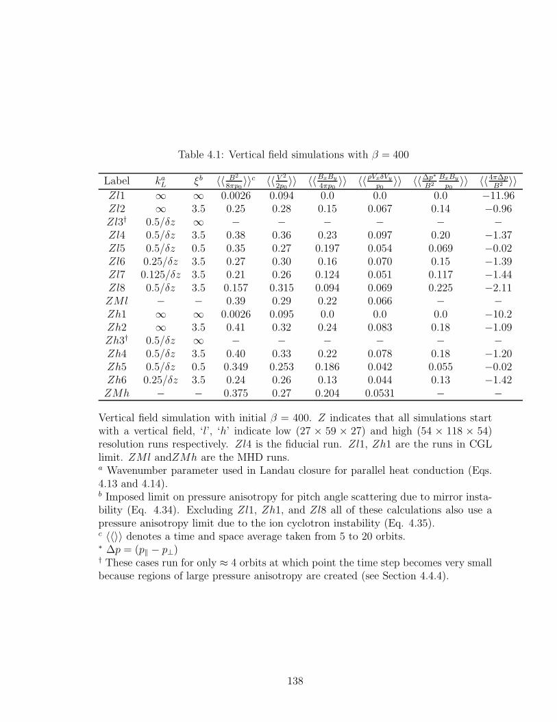
Table 4.1: Vertical field simulations with β = 400

Label kaL ξb 〈〈 B2

8πp0〉〉c 〈〈 V 2

2p0〉〉 〈〈BxBy

4πp0〉〉 〈〈ρVxδVy

p0〉〉 〈〈∆p∗

B2

BxBy

p0〉〉 〈〈4π∆p

B2 〉〉Zl1 ∞ ∞ 0.0026 0.094 0.0 0.0 0.0 −11.96Zl2 ∞ 3.5 0.25 0.28 0.15 0.067 0.14 −0.96Zl3† 0.5/δz ∞ − − − − − −Zl4 0.5/δz 3.5 0.38 0.36 0.23 0.097 0.20 −1.37Zl5 0.5/δz 0.5 0.35 0.27 0.197 0.054 0.069 −0.02Zl6 0.25/δz 3.5 0.27 0.30 0.16 0.070 0.15 −1.39Zl7 0.125/δz 3.5 0.21 0.26 0.124 0.051 0.117 −1.44Zl8 0.5/δz 3.5 0.157 0.315 0.094 0.069 0.225 −2.11ZMl − − 0.39 0.29 0.22 0.066 − −Zh1 ∞ ∞ 0.0026 0.095 0.0 0.0 0.0 −10.2Zh2 ∞ 3.5 0.41 0.32 0.24 0.083 0.18 −1.09Zh3† 0.5/δz ∞ − − − − − −Zh4 0.5/δz 3.5 0.40 0.33 0.22 0.078 0.18 −1.20Zh5 0.5/δz 0.5 0.349 0.253 0.186 0.042 0.055 −0.02Zh6 0.25/δz 3.5 0.24 0.26 0.13 0.044 0.13 −1.42ZMh − − 0.375 0.27 0.204 0.0531 − −

Vertical field simulation with initial β = 400. Z indicates that all simulations startwith a vertical field, ‘l’, ‘h’ indicate low (27 × 59 × 27) and high (54 × 118 × 54)resolution runs respectively. Zl4 is the fiducial run. Zl1, Zh1 are the runs in CGLlimit. ZMl andZMh are the MHD runs.a Wavenumber parameter used in Landau closure for parallel heat conduction (Eqs.4.13 and 4.14).b Imposed limit on pressure anisotropy for pitch angle scattering due to mirror insta-bility (Eq. 4.34). Excluding Zl1, Zh1, and Zl8 all of these calculations also use apressure anisotropy limit due to the ion cyclotron instability (Eq. 4.35).c 〈〈〉〉 denotes a time and space average taken from 5 to 20 orbits.∗ ∆p = (p‖ − p⊥)† These cases run for only ≈ 4 orbits at which point the time step becomes very smallbecause regions of large pressure anisotropy are created (see Section 4.4.4).

138

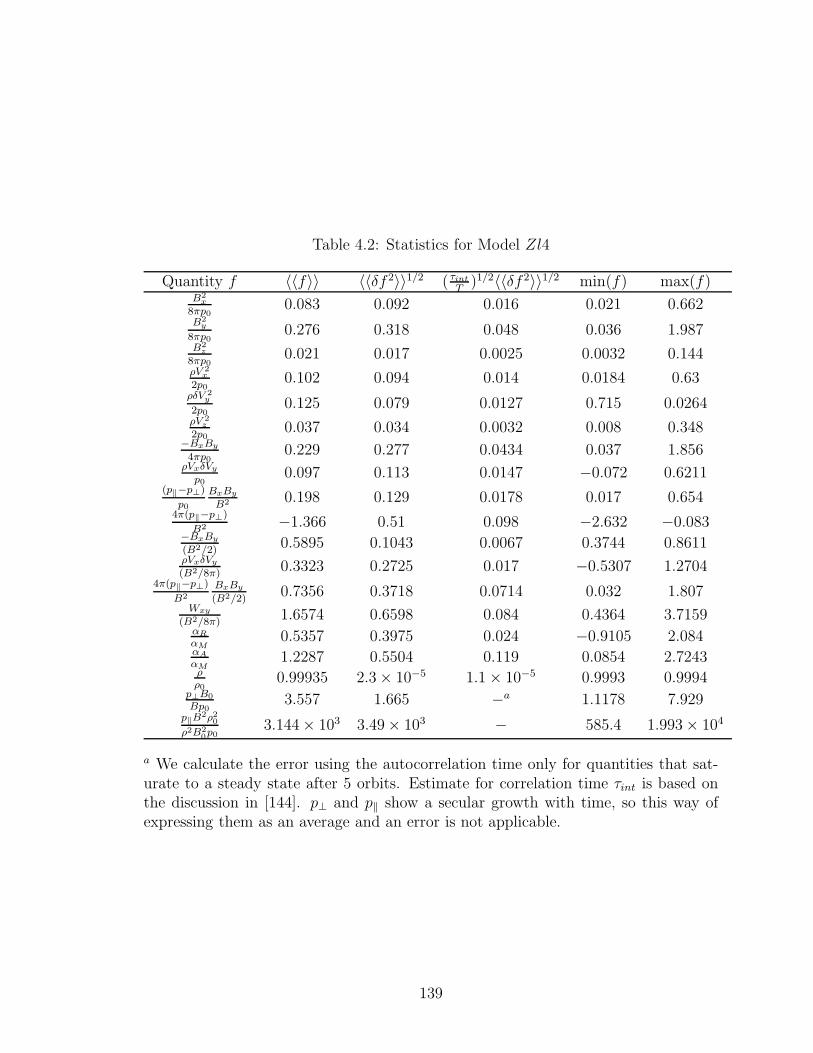
Table 4.2: Statistics for Model Zl4

Quantity f 〈〈f〉〉 〈〈δf 2〉〉1/2 ( τint

T)1/2〈〈δf 2〉〉1/2 min(f) max(f)

B2x

8πp00.083 0.092 0.016 0.021 0.662

B2y

8πp00.276 0.318 0.048 0.036 1.987

B2z

8πp00.021 0.017 0.0025 0.0032 0.144

ρV 2x

2p00.102 0.094 0.014 0.0184 0.63

ρδV 2y

2p00.125 0.079 0.0127 0.715 0.0264

ρV 2z

2p00.037 0.034 0.0032 0.008 0.348

−BxBy

4πp00.229 0.277 0.0434 0.037 1.856

ρVxδVy

p00.097 0.113 0.0147 −0.072 0.6211

(p‖−p⊥)

p0

BxBy

B2 0.198 0.129 0.0178 0.017 0.6544π(p‖−p⊥)

B2 −1.366 0.51 0.098 −2.632 −0.083−BxBy

(B2/2)0.5895 0.1043 0.0067 0.3744 0.8611

ρVxδVy

(B2/8π)0.3323 0.2725 0.017 −0.5307 1.2704

4π(p‖−p⊥)

B2

BxBy

(B2/2)0.7356 0.3718 0.0714 0.032 1.807

Wxy

(B2/8π)1.6574 0.6598 0.084 0.4364 3.7159

αR

αM0.5357 0.3975 0.024 −0.9105 2.084

αA

αM1.2287 0.5504 0.119 0.0854 2.7243

ρρ0

0.99935 2.3 × 10−5 1.1 × 10−5 0.9993 0.9994p⊥B0

Bp03.557 1.665 −a 1.1178 7.929

p‖B2ρ20

ρ2B20p0

3.144 × 103 3.49 × 103 − 585.4 1.993 × 104

a We calculate the error using the autocorrelation time only for quantities that sat-urate to a steady state after 5 orbits. Estimate for correlation time τint is based onthe discussion in [144]. p⊥ and p‖ show a secular growth with time, so this way ofexpressing them as an average and an error is not applicable.

139

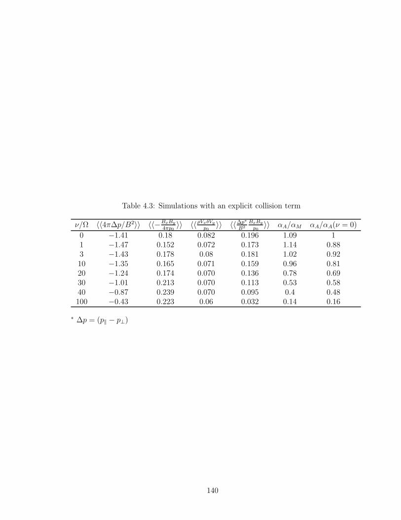
Table 4.3: Simulations with an explicit collision term

ν/Ω 〈〈4π∆p/B2〉〉 〈〈−BxBy

4πp0〉〉 〈〈ρVxδVy

p0〉〉 〈〈∆p∗

B2

BxBy

p0〉〉 αA/αM αA/αA(ν = 0)

0 −1.41 0.18 0.082 0.196 1.09 11 −1.47 0.152 0.072 0.173 1.14 0.883 −1.43 0.178 0.08 0.181 1.02 0.9210 −1.35 0.165 0.071 0.159 0.96 0.8120 −1.24 0.174 0.070 0.136 0.78 0.6930 −1.01 0.213 0.070 0.113 0.53 0.5840 −0.87 0.239 0.070 0.095 0.4 0.48100 −0.43 0.223 0.06 0.032 0.14 0.16

∗ ∆p = (p‖ − p⊥)

140

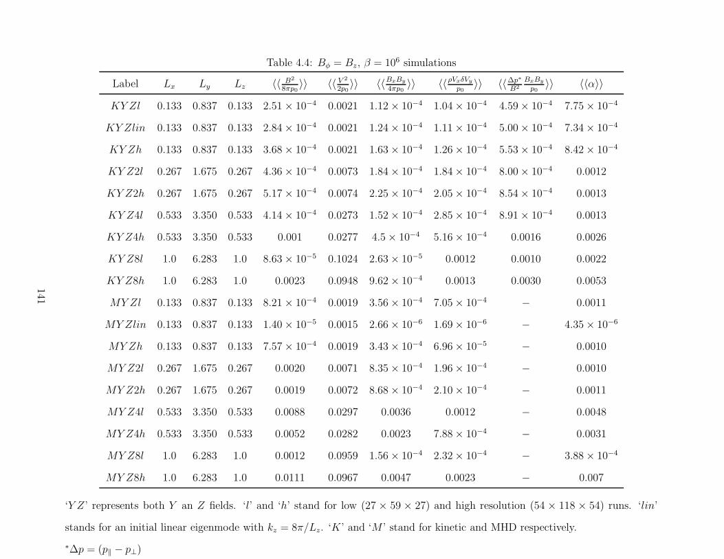
Table 4.4: Bφ = Bz, β = 106 simulations

Label Lx Ly Lz 〈〈 B2

8πp0〉〉 〈〈 V 2

2p0〉〉 〈〈BxBy

4πp0〉〉 〈〈ρVxδVy

p0〉〉 〈〈∆p∗

B2

BxBy

p0〉〉 〈〈α〉〉

KY Zl 0.133 0.837 0.133 2.51 × 10−4 0.0021 1.12 × 10−4 1.04 × 10−4 4.59 × 10−4 7.75 × 10−4

KY Zlin 0.133 0.837 0.133 2.84 × 10−4 0.0021 1.24 × 10−4 1.11 × 10−4 5.00 × 10−4 7.34 × 10−4

KY Zh 0.133 0.837 0.133 3.68 × 10−4 0.0021 1.63 × 10−4 1.26 × 10−4 5.53 × 10−4 8.42 × 10−4

KY Z2l 0.267 1.675 0.267 4.36 × 10−4 0.0073 1.84 × 10−4 1.84 × 10−4 8.00 × 10−4 0.0012

KY Z2h 0.267 1.675 0.267 5.17 × 10−4 0.0074 2.25 × 10−4 2.05 × 10−4 8.54 × 10−4 0.0013

KY Z4l 0.533 3.350 0.533 4.14 × 10−4 0.0273 1.52 × 10−4 2.85 × 10−4 8.91 × 10−4 0.0013

KY Z4h 0.533 3.350 0.533 0.001 0.0277 4.5 × 10−4 5.16 × 10−4 0.0016 0.0026

KY Z8l 1.0 6.283 1.0 8.63 × 10−5 0.1024 2.63 × 10−5 0.0012 0.0010 0.0022

KY Z8h 1.0 6.283 1.0 0.0023 0.0948 9.62 × 10−4 0.0013 0.0030 0.0053

MY Zl 0.133 0.837 0.133 8.21 × 10−4 0.0019 3.56 × 10−4 7.05 × 10−4 − 0.0011

MY Zlin 0.133 0.837 0.133 1.40 × 10−5 0.0015 2.66 × 10−6 1.69 × 10−6 − 4.35 × 10−6

MY Zh 0.133 0.837 0.133 7.57 × 10−4 0.0019 3.43 × 10−4 6.96 × 10−5 − 0.0010

MY Z2l 0.267 1.675 0.267 0.0020 0.0071 8.35 × 10−4 1.96 × 10−4 − 0.0010

MY Z2h 0.267 1.675 0.267 0.0019 0.0072 8.68 × 10−4 2.10 × 10−4 − 0.0011

MY Z4l 0.533 3.350 0.533 0.0088 0.0297 0.0036 0.0012 − 0.0048

MY Z4h 0.533 3.350 0.533 0.0052 0.0282 0.0023 7.88 × 10−4 − 0.0031

MY Z8l 1.0 6.283 1.0 0.0012 0.0959 1.56 × 10−4 2.32 × 10−4 − 3.88 × 10−4

MY Z8h 1.0 6.283 1.0 0.0111 0.0967 0.0047 0.0023 − 0.007

‘Y Z’ represents both Y an Z fields. ‘l’ and ‘h’ stand for low (27 × 59 × 27) and high resolution (54 × 118 × 54) runs. ‘lin’

stands for an initial linear eigenmode with kz = 8π/Lz. ‘K’ and ‘M ’ stand for kinetic and MHD respectively.

∗∆p = (p‖ − p⊥)

141

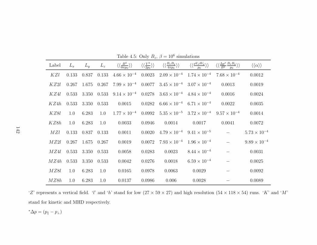
Table 4.5: Only Bz, β = 106 simulations

Label Lx Ly Lz 〈〈 B2

8πp0〉〉 〈〈 V 2

2p0〉〉 〈〈BxBy

4πp0〉〉 〈〈ρVxδVy

p0〉〉 〈〈∆p∗

B2

BxBy

p0〉〉 〈〈α〉〉

KZl 0.133 0.837 0.133 4.66 × 10−4 0.0023 2.09 × 10−4 1.74 × 10−4 7.68 × 10−4 0.0012

KZ2l 0.267 1.675 0.267 7.99 × 10−4 0.0077 3.45 × 10−4 3.07 × 10−4 0.0013 0.0019

KZ4l 0.533 3.350 0.533 9.14 × 10−4 0.0278 3.63 × 10−4 4.84 × 10−4 0.0016 0.0024

KZ4h 0.533 3.350 0.533 0.0015 0.0282 6.66 × 10−4 6.71 × 10−4 0.0022 0.0035

KZ8l 1.0 6.283 1.0 1.77 × 10−4 0.0992 5.35 × 10−5 3.72 × 10−4 9.57 × 10−4 0.0014

KZ8h 1.0 6.283 1.0 0.0033 0.0946 0.0014 0.0017 0.0041 0.0072

MZl 0.133 0.837 0.133 0.0011 0.0020 4.79 × 10−4 9.41 × 10−5 − 5.73 × 10−4

MZ2l 0.267 1.675 0.267 0.0019 0.0072 7.93 × 10−4 1.96 × 10−4 − 9.89 × 10−4

MZ4l 0.533 3.350 0.533 0.0058 0.0283 0.0023 8.44 × 10−4 − 0.0031

MZ4h 0.533 3.350 0.533 0.0042 0.0276 0.0018 6.59 × 10−4 − 0.0025

MZ8l 1.0 6.283 1.0 0.0165 0.0978 0.0063 0.0029 − 0.0092

MZ8h 1.0 6.283 1.0 0.0137 0.0986 0.006 0.0028 − 0.0089

‘Z’ represents a vertical field. ‘l’ and ‘h’ stand for low (27 × 59 × 27) and high resolution (54 × 118 × 54) runs. ‘K’ and ‘M ’

stand for kinetic and MHD respectively.

∗∆p = (p‖ − p⊥)

142

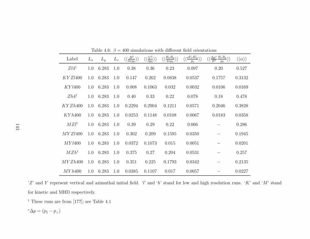
Table 4.6: β = 400 simulations with different field orientations

Label Lx Ly Lz 〈〈 B2

8πp0〉〉 〈〈 V 2

2p0〉〉 〈〈BxBy

4πp0〉〉 〈〈ρVxδVy

p0〉〉 〈〈∆p∗

B2

BxBy

p0〉〉 〈〈α〉〉

Zl4† 1.0 6.283 1.0 0.38 0.36 0.23 0.097 0.20 0.527

KY Zl400 1.0 6.283 1.0 0.147 0.262 0.0838 0.0537 0.1757 0.3132

KY l400 1.0 6.283 1.0 0.008 0.1063 0.032 0.0032 0.0106 0.0169

Zh4† 1.0 6.283 1.0 0.40 0.33 0.22 0.078 0.18 0.478

KY Zh400 1.0 6.283 1.0 0.2294 0.2904 0.1211 0.0571 0.2046 0.3828

KY h400 1.0 6.283 1.0 0.0253 0.1148 0.0108 0.0067 0.0183 0.0358

MZl† 1.0 6.283 1.0 0.39 0.29 0.22 0.066 − 0.286

MY Zl400 1.0 6.283 1.0 0.302 0.209 0.1595 0.0350 − 0.1945

MY l400 1.0 6.283 1.0 0.0372 0.1073 0.015 0.0051 − 0.0201

MZh† 1.0 6.283 1.0 0.375 0.27 0.204 0.0531 − 0.257

MY Zh400 1.0 6.283 1.0 0.351 0.225 0.1793 0.0342 − 0.2135

MY h400 1.0 6.283 1.0 0.0385 0.1107 0.017 0.0057 − 0.0227

’Z’ and Y represent vertical and azimuthal initial field. ‘l’ and ‘h’ stand for low and high resolution runs. ‘K’ and ‘M ’ stand

for kinetic and MHD respectively.

† These runs are from [177]; see Table 4.1

∗∆p = (p‖ − p⊥)

143

Chapter 5

Anisotropic conduction with large

temperature gradients

A natural step, after local studies of the MRI in the collisionless regime, is to in-

vestigate the effects of collisionless plasma processes on the global structure of colli-

sionless disks in radiatively inefficient accretion flows (RIAFs). Instead of including

both anisotropic pressure and anisotropic conduction, as in the local studies described

in Chapters 3 and 4, we began by looking at just the effects of anisotropic thermal

conduction. Anisotropic conduction is important for global disk structure because an

anisotropically conducting plasma is convectively stable if the temperature increases

outwards (dT/dr ≥ 0; see [16, 10]). Whereas, convective stability in collisional fluids

require the entropy (s = p/ργ) to increase outwards. Local, 2-D, vertically stratified

MHD simulations of Parrish and Stone [148] have confirmed that the convective insta-

bility in plasma with anisotropic thermal conduction, christened the magnetothermal

instability (MTI), is driven by temperature gradients. If convection is important,

as in hydrodynamic disks [189, 160], anisotropic conduction can modify the global

structure (and hence the luminosity) of RIAFs.

Our aim was to include anisotropic thermal conduction in global, 2-D MHD sim-

144

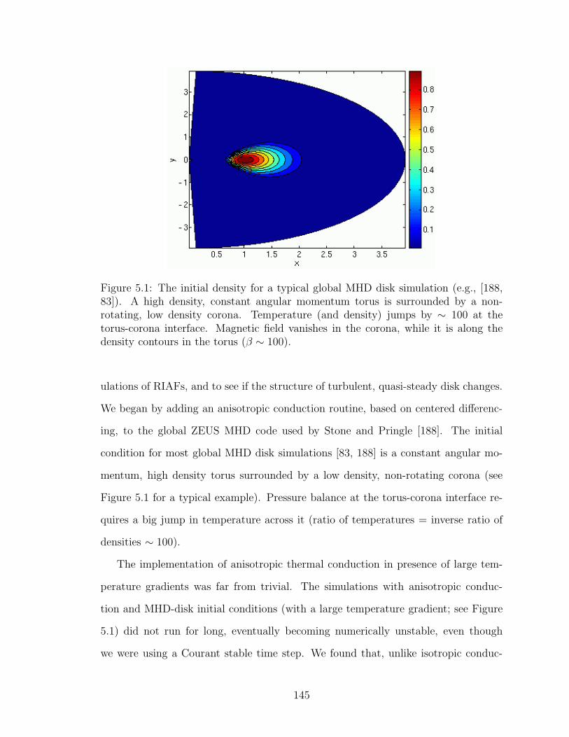
Figure 5.1: The initial density for a typical global MHD disk simulation (e.g., [188,83]). A high density, constant angular momentum torus is surrounded by a non-rotating, low density corona. Temperature (and density) jumps by ∼ 100 at thetorus-corona interface. Magnetic field vanishes in the corona, while it is along thedensity contours in the torus (β ∼ 100).

ulations of RIAFs, and to see if the structure of turbulent, quasi-steady disk changes.

We began by adding an anisotropic conduction routine, based on centered differenc-

ing, to the global ZEUS MHD code used by Stone and Pringle [188]. The initial

condition for most global MHD disk simulations [83, 188] is a constant angular mo-

mentum, high density torus surrounded by a low density, non-rotating corona (see

Figure 5.1 for a typical example). Pressure balance at the torus-corona interface re-

quires a big jump in temperature across it (ratio of temperatures = inverse ratio of

densities ∼ 100).

The implementation of anisotropic thermal conduction in presence of large tem-

perature gradients was far from trivial. The simulations with anisotropic conduc-

tion and MHD-disk initial conditions (with a large temperature gradient; see Figure

5.1) did not run for long, eventually becoming numerically unstable, even though

we were using a Courant stable time step. We found that, unlike isotropic conduc-

145

tion, the centered differencing of anisotropic conduction allowed for heat to flow from

higher to lower temperatures. The heat flow in the “wrong” direction can lead to

negative temperatures in regions with large temperature gradients. An implementa-

tion of anisotropic thermal conduction that does not give rise to negative tempera-

tures required considerable time and effort. Thus, global MHD disk simulations with

anisotropic thermal conduction have been left for the future.

Anisotropic diffusion, in which the rate of diffusion of some quantity is faster

in some directions than others, occurs in many different physical systems and ap-

plications. Examples include diffusion in geological formations, thermal properties

of structural materials and crystals, image processing [41, 136], biological systems,

and plasma physics. Diffusion Tensor Magnetic Resonance Imaging makes use of

anisotropic diffusion to distinguish different types of tissue as a medical diagnos-

tic [19]. In plasma physics, the collision operator gives rise to anisotropic diffusion in

velocity space, as does the quasilinear operator describing the interaction of particles

with waves [182]. In magnetized plasmas, thermal conduction can be much more

rapid along a field line than across it; this will be the main application in mind for

this chapter.

In this chapter we show that anisotropic thermal conduction based on centered

differences is not always consistent with the second law of thermodynamics. Test

problems that result in negative temperature with centered “asymmetric” and “sym-

metric” differencing are presented. This happens because heat can flow from lower to

higher temperature in regions with large temperature gradient. Temperature gradi-

ents in anisotropic heat fluxes need to be limited to ensure that temperature extrema

are not accentuated. We tried several different approaches, and eventually developed

slope-limited methods that successfully avoid the negative temperature problem, by

using limiters analogous to those used in numerical solution of hyperbolic equations

[116]. Perpendicular numerical diffusion (χ⊥,num) scales as ∼ χ‖∆x2 in case of the

146

least diffusive slope limited schemes. The limited methods are more diffusive than

the “symmetric” method, but comparable to the “asymmetric” method. Also, like

the “asymmetric” method, the limited methods lack the desirable property of “sym-

metric” method that the perpendicular numerical diffusion (χ⊥,num) is independent

of the parallel conduction χ‖. The main advantage of slope limited methods is that

they do not give rise to negative temperatures in presence of large temperature gra-

dients. Thus, limited methods will be useful to simulate hot, dilute astrophysical

plasmas where conduction is anisotropic and temperature gradients are enormous,

e.g., disk-corona boundary, energetic reconnection events, and collisionless shocks.

5.1 Introduction

When the plasma collision frequency, ν (∝ nT−3/2, n is the number density and T

is the temperature), is small compared to the cyclotron frequency Ωc = qB/mc, key

transport quantities like stress and thermal conduction become anisotropic with re-

spect to the magnetic field direction (the ratio of parallel to perpendicular transport

coefficients is ∼ (Ωc/ν)2); heat and momentum transport parallel to the field is much

larger than in the cross-field direction [37]. In a plasma with comparable electron and

proton temperatures, heat transport is dominated by electrons, which are faster than

ions by the ratio√

mi/me, and momentum transport is dominated by the protons.

Anisotropic plasmas are abundant in nature (e.g., solar corona, solar wind, mag-

netosphere, and radiatively inefficient accretion flows) as well as high temperature

laboratory devices like tokamaks. In order to simulate dilute, anisotropic plasmas,

accurate and robust numerical methods are needed.

Numerical methods based on finite differences [76] and higher order finite ele-

ments [181] have been useful in simulating highly anisotropic conduction (χ‖/χ⊥ ∼

109, where χ‖ and χ⊥ are parallel and perpendicular conduction coefficients) in lab-

147

oratory plasmas. “Symmetric” differencing introduced in [76] is particularly simple

and has some desirable properties—perpendicular numerical diffusion independent of

χ‖, and self adjointness of the numerical heat flux operator. The scheme based on

asymmetric centered differences, with components of the heat flux vector located at

the cell faces, have been used to study convection in anisotropically conducting plas-

mas [148] and for local simulations of collisionless accretion disks [177]. Anisotropic

thermal conduction plays a crucial role in the convective stability of dilute plasmas;

Parrish and Stone [148] have confirmed the prediction that convection in stratified

anisotropic plasmas is governed, not by the entropy gradient (the classic Schwarzchild

criterion, ds/dr > 0 for convective stability of fluids), but by the temperature gradi-

ent (dT/dr > 0 for convective stability of plasmas with anisotropic conduction; see

[10, 11]).

An important fact that has not been discussed before (to our knowledge) is that

the methods based on centered differences can give rise to heat fluxes inconsistent

with the second law of thermodynamics, i.e., heat can flow from lower to higher

temperatures! Temperature extrema can be accentuated unphysically, and negative

temperatures can arise if centered differencing is used. We show, using simple numer-

ical test problems, that both symmetric and asymmetric centered methods can give

rise to negative temperatures at some grid points. Negative temperature results in

numerical instability because the sound speed becomes imaginary.

We show that the symmetric and asymmetric methods can be modified so that

the temperature extrema are not accentuated. The components of anisotropic heat

flux, e.g., qx, consist of two contributions: the normal term, qxx = −nχb2x∂T/∂x,

and the transverse term, qxy = −nχbxby∂T/∂y. The normal term for the asymmet-

ric method, like isotropic conduction, is from higher to lower temperatures, but the

transverse term can be of any sign. The transverse term needs to be “limited” to en-

sure that temperature extrema are not accentuated. We use slope limiters, analogous

148

to those used in second order methods for hyperbolic problems [196, 116], to limit the

transverse heat fluxes. However, for the symmetric method where primary heat fluxes

are located at cell corners, qxx,i+1/2,j need not be the same sign as ∂T/∂x|i+1/2,j . Thus,

both the normal and transverse terms have to be limited for the symmetric method.

Methods based on the entropy-like function (s∗ ≡ −q · ∇T ≥ 0; see Appendix E

to see how this is different from the entropy function), which limit the transverse

component of the heat flux, are also discussed.

Limiting introduces numerical diffusion in the perpendicular direction, and the

desirable property of the symmetric method that perpendicular pollution is indepen-

dent of χ‖ no longer holds. The ratio of perpendicular numerical diffusion and the

physical parallel conductivity with a Monotonized Central (MC; see [116] for discus-

sion of slope limiters) limiter is χ⊥,num/χ‖ ∼ 10−3 for a modest number of grid points

(∼ 100 in each direction). This clearly is not adequate for simulating laboratory

plasmas which require χ‖/χ⊥ ∼ 109, as perpendicular numerical diffusion will swamp

the true perpendicular diffusion. For laboratory plasmas, the temperature profile is

relatively smooth and the negative temperature problem does not arise, so symmetric

differencing [76] or higher order finite elements [181] will be adequate.

However, astrophysical plasmas can have sharp gradients in temperature (e.g., the

transition region of the sun separating the hot corona and the much cooler chromo-

sphere, the disk-corona interface in accretion flows), and centered differencing can

give rise to negative temperatures. Thus, symmetric and asymmetric centered meth-

ods cannot be used (the sound speed becomes imaginary with negative temperature

and can give rise to spurious instabilities). The slope limited methods will intro-

duce somewhat larger perpendicular numerical diffusion (χ⊥,num/χ‖ ∼ 10−3) but will

always ensure the correct direction of heat fluxes, and hence the positivity of the

temperature. Even a modest anisotropy in conduction (χ‖/χ⊥ ∼ 103) should be

useful to study the qualitatively new effects of anisotropic conduction on dilute as-

149

trophysical plasmas, but the positivity condition on temperature is a must for robust

numerical simulations (ruling out the use of centered differencing for plasmas with

large temperature gradients). Figure 3 in [148] shows that the linear growth rate

of the magnetothermal instability (the convective instability of stratified anisotropic

plasmas discussed in [16, 10]) is not much different for χ⊥/χ‖ → 0 and χ⊥/χ‖ . 0.1,

and a numerical method that gives rise to slightly larger (compared to the symmet-

ric method, but still χ⊥,num/χ‖ < 0.1) pollution of perpendicular conduction looks

acceptable. We have tested our slope-limited methods on the magnetothermal insta-

bility and get results similar to [148], both linearly and nonlinearly.

The chapter is organized as follows. We begin with the equation for anisotropic

conduction and its numerical implementation using asymmetric and symmetric cen-

tered differencing. We present simple 2-D test problems for which asymmetric and

symmetric centered differencing give rise to negative temperatures. The slope limited

methods for anisotropic heat conduction are introduced, followed by the limiting of

the symmetric method based on the entropy-like condition. We discuss some math-

ematical properties of the slope limited methods. We present further test problems

comparing different methods and study their convergence properties. In the end we

conclude and discuss the applications of the methods that we have developed.

5.2 Anisotropic thermal conduction

Anisotropic thermal conduction can be important in a magnetized plasmas if the

mean free path (much larger than the gyroradius) is comparable to the dynamical

length scales. In such cases, a divergence of anisotropic heat flux has to be added to

the energy equation. Such a term can modify the characteristic structure of the MHD

equations and can be evolved separately by using operator splitting, as done in [148].

In operator splitting, MHD evolution operator and anisotropic thermal conduction

150

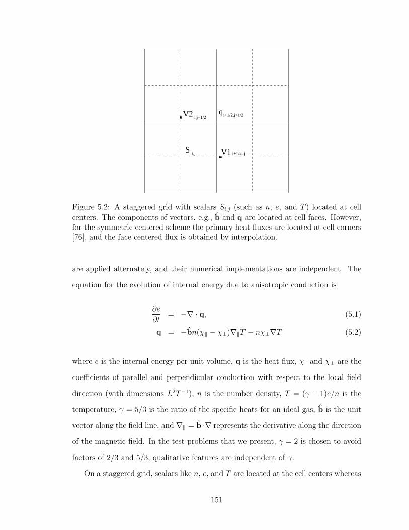
S V1i,j i+1/2, j

V2 i,j+1/2q i+1/2,j+1/2

Figure 5.2: A staggered grid with scalars Si,j (such as n, e, and T ) located at cell

centers. The components of vectors, e.g., b and q are located at cell faces. However,for the symmetric centered scheme the primary heat fluxes are located at cell corners[76], and the face centered flux is obtained by interpolation.

are applied alternately, and their numerical implementations are independent. The

equation for the evolution of internal energy due to anisotropic conduction is

∂e

∂t= −∇ · q, (5.1)

q = −bn(χ‖ − χ⊥)∇‖T − nχ⊥∇T (5.2)

where e is the internal energy per unit volume, q is the heat flux, χ‖ and χ⊥ are the

coefficients of parallel and perpendicular conduction with respect to the local field

direction (with dimensions L2T−1), n is the number density, T = (γ − 1)e/n is the

temperature, γ = 5/3 is the ratio of the specific heats for an ideal gas, b is the unit

vector along the field line, and ∇‖ = b·∇ represents the derivative along the direction

of the magnetic field. In the test problems that we present, γ = 2 is chosen to avoid

factors of 2/3 and 5/3; qualitative features are independent of γ.

On a staggered grid, scalars like n, e, and T are located at the cell centers whereas

151

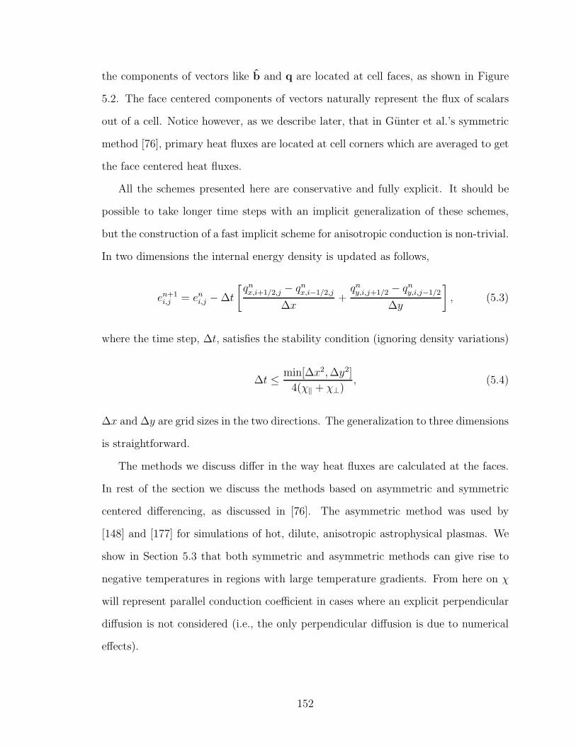
the components of vectors like b and q are located at cell faces, as shown in Figure

5.2. The face centered components of vectors naturally represent the flux of scalars

out of a cell. Notice however, as we describe later, that in Gunter et al.’s symmetric

method [76], primary heat fluxes are located at cell corners which are averaged to get

the face centered heat fluxes.

All the schemes presented here are conservative and fully explicit. It should be

possible to take longer time steps with an implicit generalization of these schemes,

but the construction of a fast implicit scheme for anisotropic conduction is non-trivial.

In two dimensions the internal energy density is updated as follows,

en+1i,j = en

i,j − ∆t

[

qnx,i+1/2,j − qn

x,i−1/2,j

∆x+qny,i,j+1/2 − qn

y,i,j−1/2

∆y

]

, (5.3)

where the time step, ∆t, satisfies the stability condition (ignoring density variations)

∆t ≤ min[∆x2,∆y2]

4(χ‖ + χ⊥), (5.4)

∆x and ∆y are grid sizes in the two directions. The generalization to three dimensions

is straightforward.

The methods we discuss differ in the way heat fluxes are calculated at the faces.

In rest of the section we discuss the methods based on asymmetric and symmetric

centered differencing, as discussed in [76]. The asymmetric method was used by

[148] and [177] for simulations of hot, dilute, anisotropic astrophysical plasmas. We

show in Section 5.3 that both symmetric and asymmetric methods can give rise to

negative temperatures in regions with large temperature gradients. From here on χ

will represent parallel conduction coefficient in cases where an explicit perpendicular

diffusion is not considered (i.e., the only perpendicular diffusion is due to numerical

effects).

152

(nχ)−1/2 (nχ)1/2

T0 T1T−1

Figure 5.3: This figure provides a motivation for using a harmonic average for nχ.Consider a 1-D case with the temperatures and nχ’s as shown in the figure. GivenT−1 and T1 and the nχ’s at the faces, we want to calculate an average nχ betweencells −1 and 1. Assumption of a constant heat flux gives, q−1/2 = q1/2 = q, i.e.,−(nχ)−1/2(T0 − T−1)/∆x = −(nχ)1/2(T1 − T0)/∆x = −nχ(T1 − T−1)/2∆x. Thisimmediately gives a harmonic mean, which is weighted towards the smaller of thetwo arguments, for the interpolation nχ.

5.2.1 Centered asymmetric scheme

The heat flux in the x- direction (in 2-D), using the asymmetric method is given by

qx,i+1/2,j = −nχbx[

bx∂T

∂x+ by

∂T

∂y

]

, (5.5)

where overline represents the variables interpolated to the face at (i + 1/2, j). The

variables without an overline are naturally located at the face. The interpolated

quantities at the face are given by simple arithmetic averaging,

by = (by,i,j−1/2 + by,i+1,j−1/2 + by,i,j+1/2 + by,i+1,j+1/2)/4, (5.6)

∂T/∂y = (Ti,j+1 + Ti+1,j+1 − Ti,j−1 − Ti+1,j−1)/4∆y. (5.7)

153

We use a harmonic mean to interpolate the product of number density and con-

ductivity,

2

nχ=

1

(nχ)i,j

+1

(nχ)i+1,j

; (5.8)

this is second order accurate for smooth regions, but nχ becomes proportional to the

minimum of the two nχ’s on either side of the face when the two differ significantly.

Figure 5.3 gives the motivation for the use of a harmonic average. Harmonic averaging

is also necessary for the method to be stable with the present time step given in Eq.

5.4. Instead, if we use a simple mean, the stable time step condition becomes severe by

a factor ∼ max[ni+1,j , ni,j]/2min[ni+1,j , ni,j], which can result in unacceptably small

time steps for initial conditions with large density contrast. Physically, this is because

the heat capacity is very small in a low density region, so a small amount of heat flow

into that region causes very fast changes in the temperature.

Analogous expressions can be written for the heat fluxes in other directions. This

method is used in astrophysical MHD simulations of [148] and [177], who include

anisotropic conduction in a cartesian geometry.

5.2.2 Centered symmetric scheme

The notion of symmetric differencing was introduced in [76], where primary heat

fluxes are located at the cell corners, with

qx,i+1/2,j+1/2 = −nχbx[

bx∂T

∂x+ by

∂T

∂y

]

, (5.9)

154

where overline represents the interpolation of variables at the corner given by a simple

arithmetic average

bx = (bx,i+1/2,j + bx,i+1/2,j+1)/2, (5.10)

by = (by,i,j+1/2 + by,i+1,j+1/2)/2, (5.11)

∂T/∂x = (Ti+1,j + Ti+1,j+1 − Ti,j − Ti,j+1)/2∆x, (5.12)

∂T/∂y = (Ti,j+1 + Ti+1,j+1 − Ti,j − Ti+1,j)/2∆y. (5.13)

As before (and for the same reasons), a harmonic average is used for the number

density

4

nχ=

1

(nχ)i,j+

1

(nχ)i+1,j+

1

(nχ)i,j+1+

1

(nχ)i+1,j+1. (5.14)

This is different from [76] who use an arithmetic average for n and χ. Analogous

expression can be written for qy,i+1/2,j+1/2.

The heat fluxes located at the cell faces, qx,i+1/2,j and qy,i,j+1/2, to be used in

Eq. (5.3) are given by an arithmetic average,

qx,i+1/2,j = (qx,i+1/2,j+1/2 + qx,i+1/2,j−1/2)/2, (5.15)

qy,i,j+1/2 = (qy,i+1/2,j+1/2 + qy,i−1/2,j+1/2)/2. (5.16)

As demonstrated in [76], the symmetric heat flux satisfies the self adjointness property

(equivalent to s∗ ≡ −q · ∇T ≥ 0 at cell corners) and has the desirable property that

the perpendicular numerical diffusion (χ⊥,num) is independent of χ‖/χ⊥. But, as we

show later, both symmetric and asymmetric schemes do not satisfy the very important

local property that heat must flow from higher to lower temperatures; the violation of

this at temperature minima can result in negative temperature in regions with large

temperature gradients.

As mentioned earlier, the heat flux in the x- direction, qx, consists of two terms,

155

+

+− −

+

+

−

− +

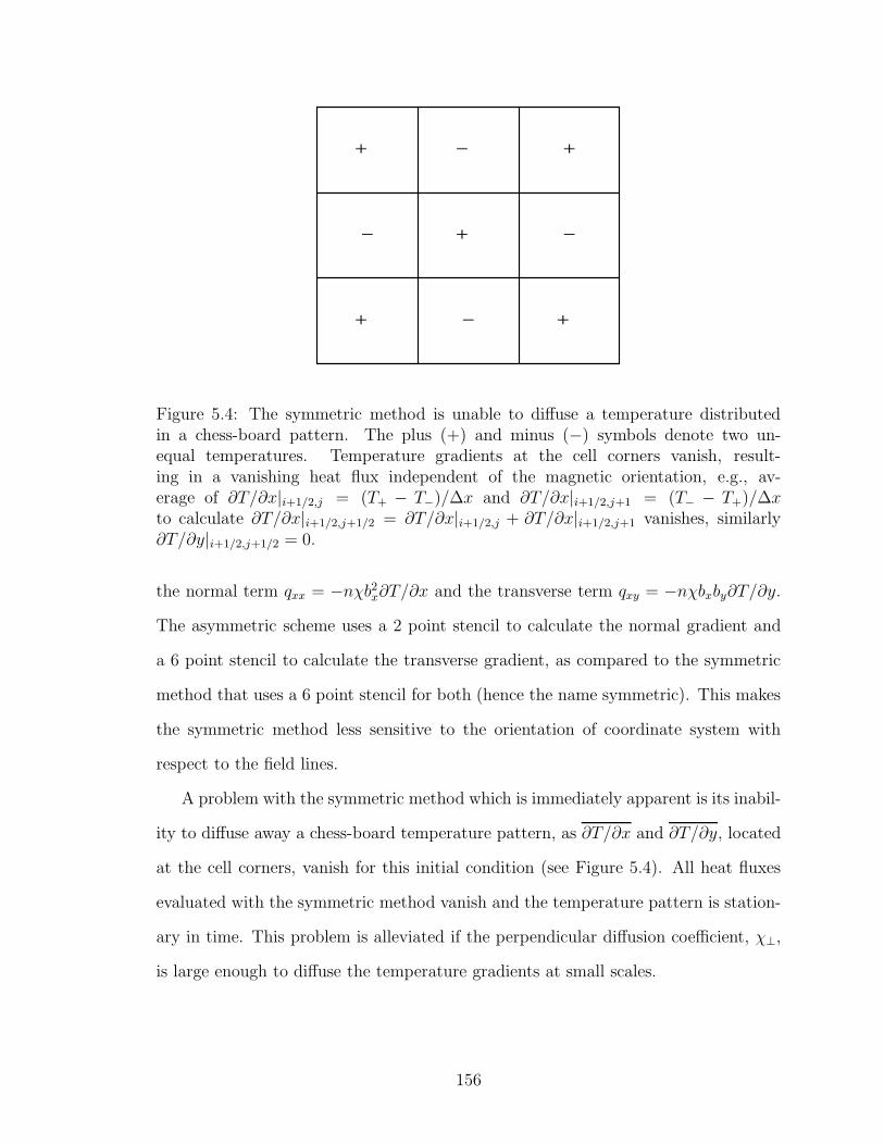
Figure 5.4: The symmetric method is unable to diffuse a temperature distributedin a chess-board pattern. The plus (+) and minus (−) symbols denote two un-equal temperatures. Temperature gradients at the cell corners vanish, result-ing in a vanishing heat flux independent of the magnetic orientation, e.g., av-erage of ∂T/∂x|i+1/2,j = (T+ − T−)/∆x and ∂T/∂x|i+1/2,j+1 = (T− − T+)/∆xto calculate ∂T/∂x|i+1/2,j+1/2 = ∂T/∂x|i+1/2,j + ∂T/∂x|i+1/2,j+1 vanishes, similarly∂T/∂y|i+1/2,j+1/2 = 0.

the normal term qxx = −nχb2x∂T/∂x and the transverse term qxy = −nχbxby∂T/∂y.

The asymmetric scheme uses a 2 point stencil to calculate the normal gradient and

a 6 point stencil to calculate the transverse gradient, as compared to the symmetric

method that uses a 6 point stencil for both (hence the name symmetric). This makes

the symmetric method less sensitive to the orientation of coordinate system with

respect to the field lines.

A problem with the symmetric method which is immediately apparent is its inabil-

ity to diffuse away a chess-board temperature pattern, as ∂T/∂x and ∂T/∂y, located

at the cell corners, vanish for this initial condition (see Figure 5.4). All heat fluxes

evaluated with the symmetric method vanish and the temperature pattern is station-

ary in time. This problem is alleviated if the perpendicular diffusion coefficient, χ⊥,

is large enough to diffuse the temperature gradients at small scales.

156

5.3 Negative temperature with centered differenc-

ing

In this section we present two simple test problems that demonstrate that negative

temperatures can arise because of centered differencing, for both asymmetric and

symmetric methods.

5.3.1 Asymmetric method

Consider a 2 × 2 grid with a hot zone (T = 10) in the first quadrant and cold

temperature (T = 0.1) in the rest, as shown in Figure 5.5. Magnetic field is uniform

over the box with bx = −by = 1/√

2. Number density is a constant equal to unity.

Reflecting boundary conditions are used. Using the asymmetric scheme for heat fluxes

out of the grid point (i, j) (the third quadrant) gives, qx,i−1/2,j = qy,i,j−1/2 = 0, and

qx,i+1/2,j = qy,i,j+1/2 = (9.9/8)nχ/∆x (where ∆x = ∆y is assumed). Thus, heat

flows out of the grid point (i, j), already a temperature minimum. This gives rise

to temperature becoming negative. Figure 5.5 shows the temperature in the third

quadrant with time for different methods. The asymmetric method gives negative

temperature (Ti,j < 0) for first few time steps, which eventually becomes positive. All

other methods (except the one based on entropy limiting) give positive temperatures

at all times for this problem. Methods based on limiting temperature gradients will

be discussed later. This test demonstrates that the asymmetric method may not be

suitable for cases with large temperature gradients because negative temperatures

result in numerical instabilities.

5.3.2 Symmetric method

The symmetric method does not give negative temperature with the test problem

of the previous section. In fact, the symmetric method gives the correct result for

157

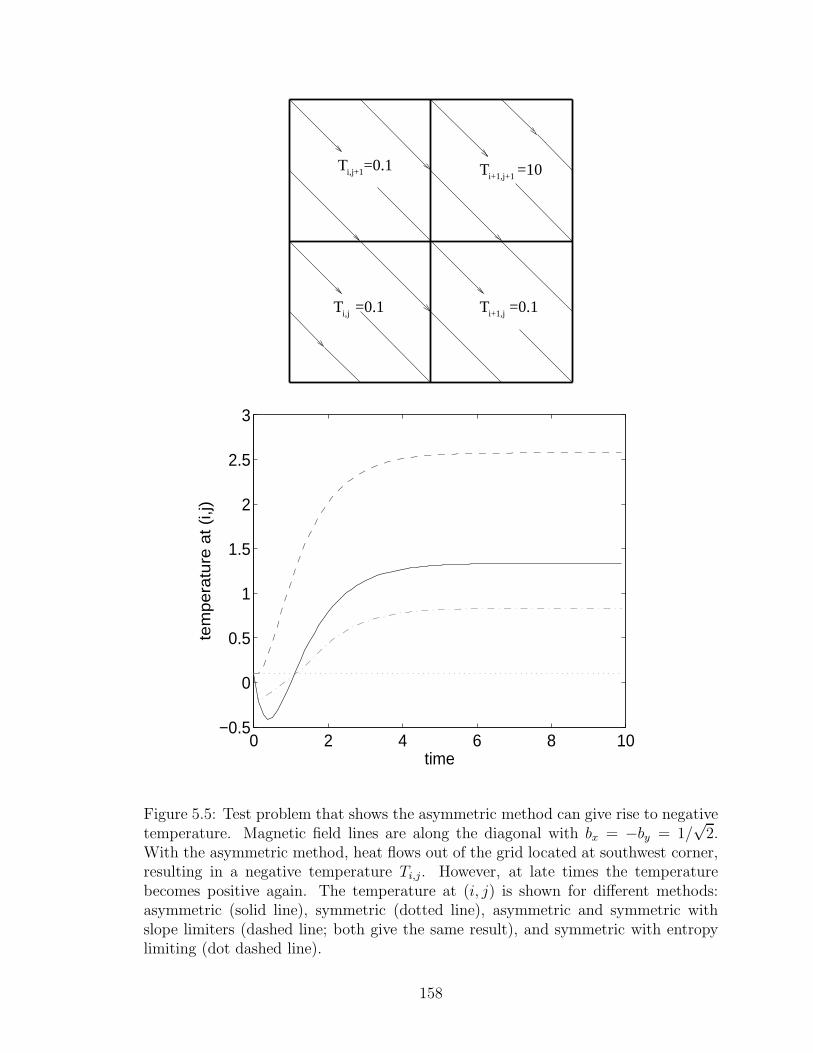
i,j+1

i,j i+1,jT =0.1

i+1,j+1T =10

T =0.1

T =0.1

0 2 4 6 8 10−0.5

0

0.5

1

1.5

2

2.5

3

time

tem

pe

ratu

re a

t (i,j)

Figure 5.5: Test problem that shows the asymmetric method can give rise to negativetemperature. Magnetic field lines are along the diagonal with bx = −by = 1/

√2.

With the asymmetric method, heat flows out of the grid located at southwest corner,resulting in a negative temperature Ti,j. However, at late times the temperaturebecomes positive again. The temperature at (i, j) is shown for different methods:asymmetric (solid line), symmetric (dotted line), asymmetric and symmetric withslope limiters (dashed line; both give the same result), and symmetric with entropylimiting (dot dashed line).

158

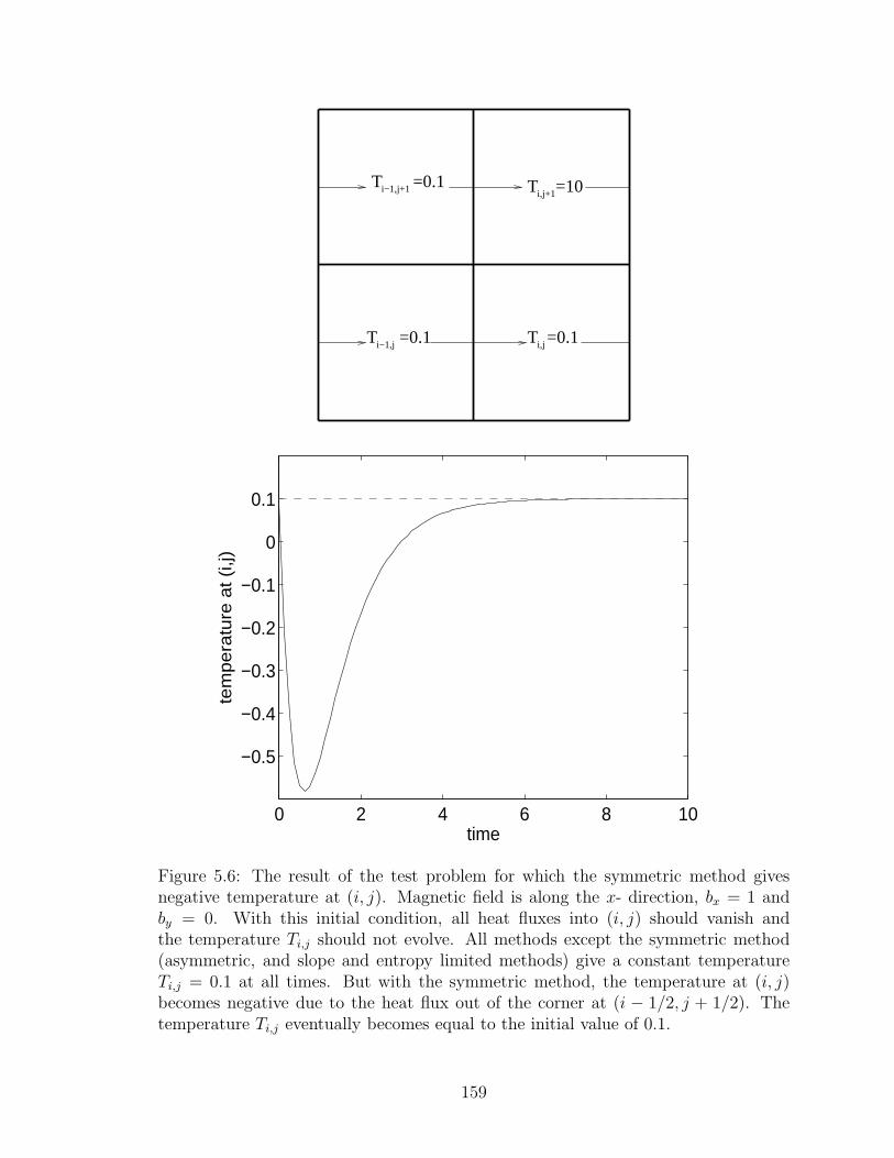
i,jT =0.1i−1,j

i−1,j+1

T =0.1

i,j+1T =10T =0.1

0 2 4 6 8 10

−0.5

−0.4

−0.3

−0.2

−0.1

0

0.1

time

tem

pe

ratu

re a

t (i,j)

Figure 5.6: The result of the test problem for which the symmetric method givesnegative temperature at (i, j). Magnetic field is along the x- direction, bx = 1 andby = 0. With this initial condition, all heat fluxes into (i, j) should vanish andthe temperature Ti,j should not evolve. All methods except the symmetric method(asymmetric, and slope and entropy limited methods) give a constant temperatureTi,j = 0.1 at all times. But with the symmetric method, the temperature at (i, j)becomes negative due to the heat flux out of the corner at (i − 1/2, j + 1/2). Thetemperature Ti,j eventually becomes equal to the initial value of 0.1.

159

temperature with no numerical diffusion in the perpendicular direction (zero heat flux

out of the grid point (i, j), see Figure 5.5). Other methods resulted in a temperature

increase at (i, j) because of perpendicular numerical diffusion. Here we consider a

case where the symmetric method gives negative temperature.

As before, consider a 2 × 2 grid with a hot zone (T = 10) in the first quadrant

and cold temperature (T = 0.1) in the rest; the only difference from the previous

test problem is that the magnetic field lines are along the x- axis, bx = 1 and by = 0

(see Figure 5.6). Reflective boundary conditions are used, as before. Since there

is no temperature gradient along the field lines for the grid point (i, j), we do not

expect the temperature there to change. While all other methods give a stationary

temperature in time, the symmetric method results in a heat flux out of the grid

(i, j) through the corner at (i− 1/2, j + 1/2). With the initial condition as shown in

Figure 5.6, the only non-vanishing symmetric heat flux out of (i, j) is, qx,i−1/2,j+1/2 =

−(9.9/2)nχ∆x. The only non-vanishing face-centered heat flux entering the box

through a face is qx,i−1/2,j = −(9.9/4)nχ∆x < 0; i.e., heat flows out of (i, j) which is

already a temperature minimum. This results in the temperature becoming negative

at (i, j), although at late times it becomes equal to the initial temperature at (i, j).

This simple test shows that the symmetric method can give negative temperatures

(and associated numerical problems) in presence of large temperature gradients.

5.4 Slope limited fluxes

The heat flux qx is composed of two terms, the normal qxx = −nχb2x∂T/∂x term, and

the transverse qxy = −nχbxby∂T/∂y term. For the asymmetric method, the discrete

form of the term qxx = −nχb2x∂T/∂x is of the same sign as the x- component of

isotropic heat flux (−nχ∂T/∂x), and hence it guarantees that heat flows from higher

to lower temperatures. However, qxy = −nχbxby∂T/∂y can have an arbitrary sign,

160

and can give rise to heat flowing in the “wrong” direction. We use slope limiters,

analogous to those used for linear reconstruction of variables in numerical simulation

of hyperbolic systems [196, 116], to “limit” the transverse terms. Both asymmet-

ric and symmetric methods can be modified with slope limiters. The slope limited

heat fluxes ensure that temperature extrema are not accentuated. Thus, unlike the

symmetric and asymmetric methods, slope limited methods can never give negative

temperatures.

5.4.1 Limiting the asymmetric method

Since the normal heat flux term, qxx, is naturally located at the face, no interpolation

for ∂T/∂x is required for its evaluation. However, an interpolation at the x- face

is required to evaluate ∂T/∂y used in qxy (the term with overlines in Eq. 5.5).

The arithmetic average used in Eq. 5.7 for ∂T/∂y to calculate qxy was found to

result in heat flowing from lower to higher temperatures (see Figure 5.5). To remedy

this problem we have used slope limiters to interpolate temperature gradients in the

transverse heat fluxes.

Slope limiters are widely used in numerical simulations of hyperbolic equations

(e.g., computational gas dynamics; see [196, 116]). Given the initial values for vari-

ables at grid centers, slope limiters (e.g., minmod, van Leer, and Monotonized Central

(MC)) are used to calculate the slopes of conservative piecewise linear reconstructions

in each grid cell. Limiters use the variable values in the nearest grid cells to come up

with slopes which ensure that no new extrema are created for conserved variables, a

property of hyperbolic equations. We use slope limiters to interpolate temperature

gradients in transverse heat flux terms. Analogous to hyperbolic problems where lim-

iters prevent new unphysical extrema, limiters prevent amplification of temperature

extrema; this may result in negative temperatures.

The slope limited asymmetric heat flux in the x- direction is still given by Eq. 5.5,

161

with the same ∂T/∂x as in the asymmetric method, but a slope limited interpolation

for the transverse temperature gradient, ∂T/∂y is needed,

∂T

∂y

∣

∣

∣

∣

i+1/2,j

= L

L

[

∂T

∂y

∣

∣

∣

∣

i,j−1/2

,∂T

∂y

∣

∣

∣

∣

i,j+1/2

]

, L

[

∂T

∂y

∣

∣

∣

∣

i+1,j−1/2

,∂T

∂y

∣

∣

∣

∣

i+1,j+1/2

]

,

(5.17)

where L is a slope limiter like minmod, van Leer, or Monotonized Central (MC)

limiter [116]; e.g., the van Leer limiter is

L(a, b) =2ab

a+ bif ab > 0,

= 0 otherwise. (5.18)

Slope limiters weights the interpolation towards the argument smallest in magnitude,

and returns a zero if the two arguments are of opposite signs. An analogous expression

for the transverse temperature gradient at the y- face, ∂T/∂x, is used to evaluate

the heat flux qy. Averaging similar to the asymmetric method is used for all other

interpolations (Eqs. 5.6 and 5.8).

5.4.2 Limiting the symmetric method

In the symmetric method, primary heat fluxes in both directions are located at the

cell corners (see Eq. 5.9). Temperature gradients in both directions have to be inter-

polated at the corners. Thus, to ensure that temperature extrema are not amplified

with the symmetric method, both ∂T/∂x and ∂T/∂y need to be limited.

The face-centered qxx,i+1/2,j is calculated by averaging qxx from the adjacent cor-

162

ners, which are given by the following slope-limited expressions:

qNxx,i+1/2,j+1/2 = −nχb2xL2

[

∂T

∂x

∣

∣

∣

∣

i+1/2,j

,∂T

∂x

∣

∣

∣

∣

i+1/2,j+1

]

, (5.19)

qSxx,i+1/2,j−1/2 = −nχb2xL2

[

∂T

∂x

∣

∣

∣

∣

i+1/2,j

,∂T

∂x

∣

∣

∣

∣

i+1/2,j−1

]

, (5.20)

where S and N superscripts indicate the south-biased corner heat flux or the north-

biased heat flux. The face centered heat flux used in Eq. 5.3 is qxx,i+1/2,j = (qNxx,i+1/2,j+1/2+

qSxx,i+1/2,j−1/2)/2; the interpolated quantities (indicated with an overline) are the same

as in Eq. 5.9. The limiter L2, which is somewhat different from standard slope lim-

iters, is defined as

L2(a, b) = (a+ b)/2, if min(αa, a/α) < (a + b)/2 < max(αa, a/α),

= min(αa, a/α), if (a + b)/2 ≤ min(αa, a/α),

= max(αa, a/α), if (a + b)/2 ≥ max(αa, a/α), (5.21)

where 0 < α < 1 is a parameter; this reduces to a simple averaging if the temperature

is smooth while restricting the interpolated temperature (∂T/∂x) to not differ too

much from ∂T/∂x|i+1/2,j (and be of the same sign). We choose α = 3/4; results are

not very sensitive to the exact value of α. The L2 limiter is not symmetric with

respect to its arguments (and thus the definition of qSxx,i+1/2,j+1/2 is slightly different

than the definition of qNxx,i+1/2,j+1/2). It ensures that qxx,i+1/2,j±1/2 is of the same sign

as −∂T/∂x|i+1/2,j ; i.e., the interpolated normal heat flux flows from higher to lower

temperatures. If we use a standard slope limiter (e.g., minmod, van Leer, or MC) in

Eqs. 5.19 and 5.20, for the chessboard pattern shown in Figure 5.4, all heat fluxes

vanish as with the symmetric method. However, the L2 limiter gives,

qxx,i+1/2,j+1/2 = qxx,i+1/2,j−1/2 = −nχbx2α∂T

∂x

∣

∣

∣

∣

i+1/2,j

,

163

a heat flux from higher to lower temperatures which can diffuse the chessboard pat-

tern.

The transverse temperature gradient is limited in a way similar to the asymmetric

method. The temperature gradient ∂T/∂y to be used in Eq. 5.9 is given by

∂T

∂y

∣

∣

∣

∣

i+1/2,j+1/2

= L

[

∂T

∂y

∣

∣

∣

∣

i+1,j+1/2

,∂T

∂y

∣

∣

∣

∣

i,j+1/2

]

, (5.22)

with qxy,i+1/2,j = L(qxy,i+1/2,j+1/2, qxy,i+1/2,j−1/2), where L is a standard slope limiter.

5.5 Limiting using the entropy-like source func-

tion

If the entropy-like source function, which we define as s∗ = −q · ∇T (see Appendix

E to see how this is different from the entropy function), is positive at all spatial

locations, heat is guaranteed to flow from higher to lower temperatures. For the

symmetric method, s∗ evaluated at the cell corners is positive definite, but need not

be positive definite if evaluated at the cell faces, and thus allows the heat to flow across

faces from lower to higher temperatures. This can cause temperature to decrease at

a minimum; temperature can also become negative if temperature gradients are large

(see Figure 5.6). Thus, s∗ ≥ 0 satisfied at all corners on the grid is not sufficient for

the heat to flow from higher to lower temperatures. We use the following entropy-like

condition, applied at all face-pairs, to limit the transverse heat flux terms (qxy and

qyx)

s∗ = −qx,i+1/2,j∂T

∂x

∣

∣

∣

∣

i+1/2,j

− qy,i,j+1/2∂T

∂y

∣

∣

∣

∣

i,j+1/2

≥ 0. (5.23)

The limiter L2 is used to calculate the normal gradients qxx and qyy at the faces, as

in the slope limited symmetric method. The use of L2 ensures that −qxx,i+1/2,j∂T/∂x|i+1/2,j ≥

0, and only the transverse terms qxy and qyx need to be reduced to satisfy Eq. 5.23.

164

That is, if on evaluating s∗ the entropy-like condition (Eq. 5.23) is violated, the

transverse terms are reduced to make s∗ vanish. The attractive feature of the entropy

limited symmetric method is that it reduces to the symmetric method (least diffusive

of all the methods; see Figure 5.9) when Eq. 5.23 is satisfied, and the limiting of

transverse terms may help with the amplification of temperatures at extrema.

The problem with entropy limiting is that the temperature extrema can still be am-

plified (see Figures 5.5 and 5.8). For example, when ∂T/∂x|i+1/2,j = ∂T/∂y|i,j+1/2 =

0, Eq. 5.23 is satisfied for arbitrary heat fluxes qx,i+1/2,j and qy,i,j+1/2. In such a case,

transverse heat fluxes qxy and qyx can cause heat to flow across the zero temperature

gradient and result in a new temperature extremum, which may even be a nega-

tive. However, this unphysical behavior can only occur for one time step, after which

∇T 6= 0 and Eq. 5.23 becomes a useful limit again. The result is that the overshoots

are not as pronounced as in the asymmetric and symmetric methods, as shown in

Figures 5.7 and 5.8. With entropy limiting, unlike the symmetric and asymmetric

methods, the spurious temperature oscillations (reminiscent of unphysical oscillations

near discontinuities in hyperbolic systems) are damped (see Figure 5.8). Although

temperature minimum can be accentuated by the entropy limited method, early on

one can choose sufficiently small time steps to ensure that temperature does not be-

come negative; this is equivalent to saying that entropy limited method will not give

negative temperatures at late times (see Figure 5.8 and Tables 5.1-5.4). This trick will

not work for the centered symmetric and asymmetric methods where temperatures

can be negative even at late times (see Figure 5.8).

To guarantee that temperature extrema are not amplified, in addition to entropy

limiting at all points, one should also use slope limiting of transverse temperature

gradients at extrema. This results in a method that does not amplify the extrema,

but is more diffusive compared to just entropy limiting (see Figure 5.9). Because of

simplicity of slope limited methods and their desirable mathematical properties (dis-

165

cussed in the next section), they are preferred over the cumbersome entropy limited

methods.

5.6 Mathematical properties

In this section we prove that the slope limited fluxes do not amplify the temperature

extrema. Also discussed are global and local properties related to the entropy-like

condition, s∗ = −q · ∇T ≥ 0.

5.6.1 Behavior at temperature extrema

Slope limiting of both asymmetric and symmetric methods guarantees that the tem-

perature extrema are not amplified further, i.e., the maximum temperature does not

increase and the minimum does not decrease. This ensures that the temperature is

always positive and numerical problems because of imaginary sound speed do not

arise. The normal heat flux in the asymmetric method (= −nχb2x∂T/∂x) and the L2

limited normal heat flux term in the symmetric method (Eqs. 5.19 and 5.20) allows

the heat to flow only from higher to lower temperatures. Thus, the terms responsible

for unphysical behavior at temperature extrema are the transverse heat fluxes qxy and

qyx. Slope limiters ensure that the transverse heat terms vanish at extrema and heat

flows down the temperature gradient at those grid points.

The operator L(L(a, b), L(c, d)), where L is a slope limiter like minmod, van Leer,

or MC, is symmetric with respect to all its arguments, and hence can be written

as L(a, b, c, d). For the slope limiters considered here (minmod, van Leer, and MC),

L(a, b, c, d) vanishes unless all four arguments a, b, c, d have the same sign.

At a local temperature extremum (say at (i, j)), the x- (and y-) face-centered

slopes ∂T/∂y|i,j+1/2 and ∂T/∂y|i,j−1/2 (and ∂T/∂x|i+1/2,j and ∂T/∂x|i−1/2,j) are of

opposite signs or at least one of them is zero. This ensures that the slope lim-

166

ited transverse temperature gradients (∂T/∂y and ∂T/∂x) vanish (from Eqs. 5.17

and 5.22). The heat fluxes become qx,i±1/2,j = −nχbx2∂T/∂x|i±1/2,j and qy,i,j±1/2 =

−nχby2∂T/∂y|i,j±1/2 at the temperature extrema, which are always down the tem-

perature gradient. This ensures that temperature never becomes negative, unlike the

methods based on centered differencing.

5.6.2 The entropy-like condition, s∗ = −q · ∇T ≥ 0

If the number density, n, remains constant in time, then multiplying Eq. 5.1 with T

and integrating over all space gives

1

(γ − 1)

∂

∂t

∫

nT 2dV = −∫

T∇ · qdV =

∫

q · ∇TdV = −∫

nχ|∇‖T |2dV ≤ 0,

(5.24)

assuming that the surface contributions vanish. This analytic constraint implies that

temperature fluctuations cannot increase in time (on an average).

Gunter et al. [76] have shown that the symmetric method is self-adjoint and

satisfies the entropy-like condition, Eq. 5.24. The local entropy-like source function

s∗ = −q · ∇T evaluated at the corner (i+ 1/2, j + 1/2) for the symmetric method is

s∗i+1/2,j+1/2 = −qx,i+1/2,j+1/2∂T

∂x

∣

∣

∣

∣

i+1/2,j+1/2

− qy,i+1/2,j+1/2∂T

∂y

∣

∣

∣

∣

i+1/2,j+1/2

. (5.25)

Using the form for symmetric heat fluxes (Eq. 5.9), the entropy-like function becomes,

s∗ = nχbx2∂T

∂x

2

+ nχby2∂T

∂y

2

+ 2nχbx by∂T

∂x

∂T

∂y,

= nχ

[

bx∂T

∂x+ by

∂T

∂y

]2

≥ 0. (5.26)

Thus, q · ∇T ≤ 0, and integration over the whole space implies Eq. 5.24. Although

the entropy-like condition is satisfied by the symmetric method at the corners (both

167

locally and globally), this condition is not sufficient to guarantee local positivity of

temperature at cell centers, as we demonstrate in Subsection 5.3.2. Also notice that

the modification of the symmetric method to satisfy entropy-like condition at face

pairs (see Section 5.5) does not cure the problem of negative temperature. Thus,

a method which satisfy the entropy-like condition (s∗ = −q · ∇T ≥ 0) does not

necessarily satisfy the condition that temperature extrema should not be amplified.

With an appropriate interpolation, the asymmetric method and the slope limited

asymmetric methods can be shown to satisfy the global entropy-like condition, S∗ =

−∫

q · ∇TdV/V ≥ 0. Consider

S∗ =−1

NxNy

∑

i,j

[

qx,i+1/2,j∂T

∂x

∣

∣

∣

∣

i+1/2,j

+ qy,i,j+1/2∂T

∂y

∣

∣

∣

∣

i,j+1/2

]

, (5.27)

where Nx and Ny are the number of grid points in each direction. Substituting the

form of asymmetric heat fluxes,

S∗ =1

NxNy

∑

i,j

(

nχb2x

∣

∣

∣

∣

∂T

∂x

∣

∣

∣

∣

2)

i+1/2,j

+

(

nχb2y

∣

∣

∣

∣

∂T

∂y

∣

∣

∣

∣

2)

i,j+1/2

+

(

nχbxby∂T

∂y

)

i+1/2,j

∂T

∂x

∣

∣

∣

∣

i+1/2,j

+

(

nχbxby∂T

∂x

)

i,j+1/2

∂T

∂y

∣

∣

∣

∣

i,j+1/2

]

,(5.28)

where overlines represent appropriate interpolations. We define

Gx,i+1/2,j =√

(nχ)i+1/2,jbx,i+1/2,j∂T

∂x

∣

∣

∣

∣

i+1/2,j

, (5.29)

Gy,i,j+1/2 =√

(nχ)i,j+1/2by,i,j+1/2∂T

∂y

∣

∣

∣

∣

i,j+1/2

, (5.30)

Gy,i+1/2,j =√nχby

∂T

∂y

∣

∣

∣

∣

i+1/2,j

, (5.31)

Gx,i,j+1/2 =√nχbx

∂T

∂x

∣

∣

∣

∣

i,j+1/2

. (5.32)

168

In terms of G’s, Eq. 5.28 can be written as

S∗ =1

NxNy

∑

i,j

[

G2x,i+1/2,j +G2

y,i,j+1/2 +Gx,i+1/2,jGy,i+1/2,j +Gy,i,j+1/2Gy,i,j+1/2

]

.

(5.33)

A lower bound on S∗ is obtained by assuming the cross terms to be negative, i.e.,

S∗ ≥ 1

NxNy

∑

i,j

[

G2x,i+1/2,j +G2

y,i,j+1/2 −∣

∣Gx,i+1/2,jGy,i+1/2,j

∣

∣−∣

∣Gy,i,j+1/2Gy,i,j+1/2

∣

∣

]

.

(5.34)

Now define Gy,i+1/2,j and Gx,i,j+1/2 as follows (the following interpolation is necessary

for the proof to hold):

Gy,i+1/2,j = L(Gy,i,j+1/2, Gy,i,j−1/2, Gy,i+1,j+1/2, Gy,i+1,j−1/2), (5.35)

Gx,i,j+1/2 = L(Gx,i+1/2,j , Gx,i−1/2,j, Gx,i+1/1,j+1, Gy,i−1/2,j+1), (5.36)

where L is an arithmetic average (as in centered asymmetric method) or a slope limiter

(e.g., minmod, van Leer, or MC) which satisfy the property that |L(a, b, c, d)| ≤

(|a| + |b| + |c| + |d|)/4, to put a lower bound on S∗. Thus,

S∗ ≥ 1

NxNy

∑

i,j

G2x,i+1/2,j +G2

y,i,j+1/2 −1

4

[∣

∣Gx,i+1/2,jGy,i,j+1/2

∣

∣

+∣

∣Gx,i+1/2,jGy,i,j−1/2

∣

∣ +∣

∣Gx,i+1/2,jGy,i+1,j+1/2

∣

∣+∣

∣Gx,i+1/2,jGy,i+1,j−1/2

∣

∣

+∣

∣Gy,i,j+1/2Gx,i+1/2,j

∣

∣ +∣

∣Gy,i,j+1/2Gx,i−1/2,j

∣

∣+∣

∣Gy,i,j+1/2Gx,i+1/2,j+1

∣

∣

+∣

∣Gy,i,j+1/2Gx,i−1/2,j+1

∣

∣

]

. (5.37)

169

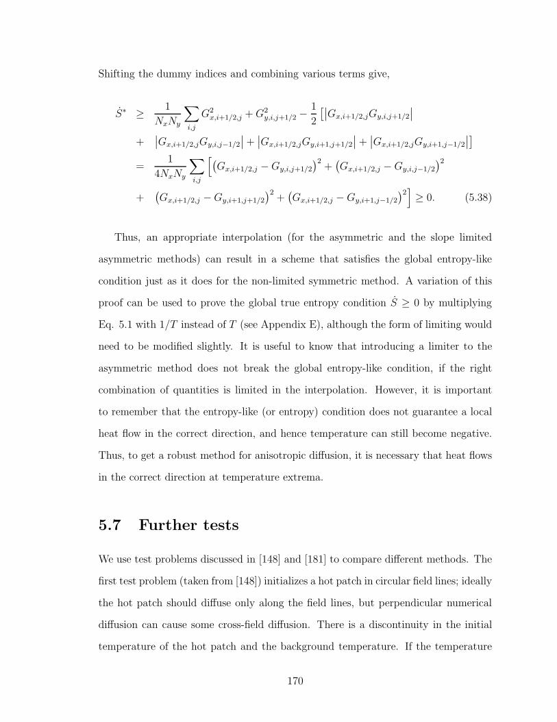
Shifting the dummy indices and combining various terms give,

S∗ ≥ 1

NxNy

∑

i,j

G2x,i+1/2,j +G2

y,i,j+1/2 −1

2

[∣

∣Gx,i+1/2,jGy,i,j+1/2

∣

∣

+∣

∣Gx,i+1/2,jGy,i,j−1/2

∣

∣+∣

∣Gx,i+1/2,jGy,i+1,j+1/2

∣

∣ +∣

∣Gx,i+1/2,jGy,i+1,j−1/2

∣

∣

]

=1

4NxNy

∑

i,j

[

(

Gx,i+1/2,j −Gy,i,j+1/2

)2+(

Gx,i+1/2,j −Gy,i,j−1/2

)2

+(

Gx,i+1/2,j −Gy,i+1,j+1/2

)2+(

Gx,i+1/2,j −Gy,i+1,j−1/2

)2]

≥ 0. (5.38)

Thus, an appropriate interpolation (for the asymmetric and the slope limited

asymmetric methods) can result in a scheme that satisfies the global entropy-like

condition just as it does for the non-limited symmetric method. A variation of this

proof can be used to prove the global true entropy condition S ≥ 0 by multiplying

Eq. 5.1 with 1/T instead of T (see Appendix E), although the form of limiting would

need to be modified slightly. It is useful to know that introducing a limiter to the

asymmetric method does not break the global entropy-like condition, if the right

combination of quantities is limited in the interpolation. However, it is important

to remember that the entropy-like (or entropy) condition does not guarantee a local

heat flow in the correct direction, and hence temperature can still become negative.

Thus, to get a robust method for anisotropic diffusion, it is necessary that heat flows

in the correct direction at temperature extrema.

5.7 Further tests

We use test problems discussed in [148] and [181] to compare different methods. The

first test problem (taken from [148]) initializes a hot patch in circular field lines; ideally

the hot patch should diffuse only along the field lines, but perpendicular numerical

diffusion can cause some cross-field diffusion. There is a discontinuity in the initial

temperature of the hot patch and the background temperature. If the temperature

170

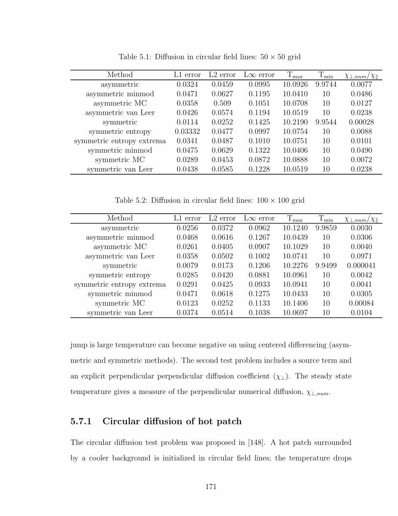
Table 5.1: Diffusion in circular field lines: 50 × 50 grid

Method L1 error L2 error L∞ error Tmax Tmin χ⊥,num/χ‖

asymmetric 0.0324 0.0459 0.0995 10.0926 9.9744 0.0077asymmetric minmod 0.0471 0.0627 0.1195 10.0410 10 0.0486

asymmetric MC 0.0358 0.509 0.1051 10.0708 10 0.0127asymmetric van Leer 0.0426 0.0574 0.1194 10.0519 10 0.0238

symmetric 0.0114 0.0252 0.1425 10.2190 9.9544 0.00028symmetric entropy 0.03332 0.0477 0.0997 10.0754 10 0.0088

symmetric entropy extrema 0.0341 0.0487 0.1010 10.0751 10 0.0101symmetric minmod 0.0475 0.0629 0.1322 10.0406 10 0.0490

symmetric MC 0.0289 0.0453 0.0872 10.0888 10 0.0072symmetric van Leer 0.0438 0.0585 0.1228 10.0519 10 0.0238

Table 5.2: Diffusion in circular field lines: 100 × 100 grid

Method L1 error L2 error L∞ error Tmax Tmin χ⊥,num/χ‖

asymmetric 0.0256 0.0372 0.0962 10.1240 9.9859 0.0030asymmetric minmod 0.0468 0.0616 0.1267 10.0439 10 0.0306

asymmetric MC 0.0261 0.0405 0.0907 10.1029 10 0.0040asymmetric van Leer 0.0358 0.0502 0.1002 10.0741 10 0.0971

symmetric 0.0079 0.0173 0.1206 10.2276 9.9499 0.000041symmetric entropy 0.0285 0.0420 0.0881 10.0961 10 0.0042

symmetric entropy extrema 0.0291 0.0425 0.0933 10.0941 10 0.0041symmetric minmod 0.0471 0.0618 0.1275 10.0433 10 0.0305

symmetric MC 0.0123 0.0252 0.1133 10.1406 10 0.00084symmetric van Leer 0.0374 0.0514 0.1038 10.0697 10 0.0104

jump is large temperature can become negative on using centered differencing (asym-

metric and symmetric methods). The second test problem includes a source term and

an explicit perpendicular perpendicular diffusion coefficient (χ⊥). The steady state

temperature gives a measure of the perpendicular numerical diffusion, χ⊥,num.

5.7.1 Circular diffusion of hot patch

The circular diffusion test problem was proposed in [148]. A hot patch surrounded

by a cooler background is initialized in circular field lines; the temperature drops

171

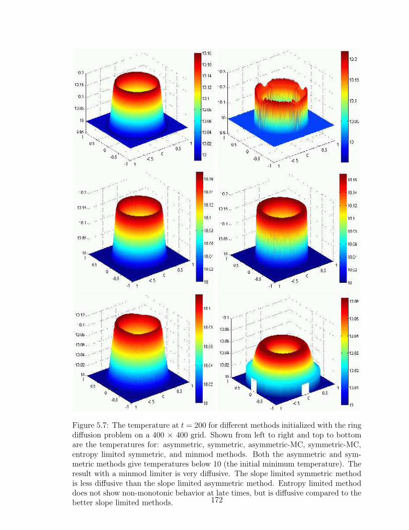
Figure 5.7: The temperature at t = 200 for different methods initialized with the ringdiffusion problem on a 400 × 400 grid. Shown from left to right and top to bottomare the temperatures for: asymmetric, symmetric, asymmetric-MC, symmetric-MC,entropy limited symmetric, and minmod methods. Both the asymmetric and sym-metric methods give temperatures below 10 (the initial minimum temperature). Theresult with a minmod limiter is very diffusive. The slope limited symmetric methodis less diffusive than the slope limited asymmetric method. Entropy limited methoddoes not show non-monotonic behavior at late times, but is diffusive compared to thebetter slope limited methods. 172

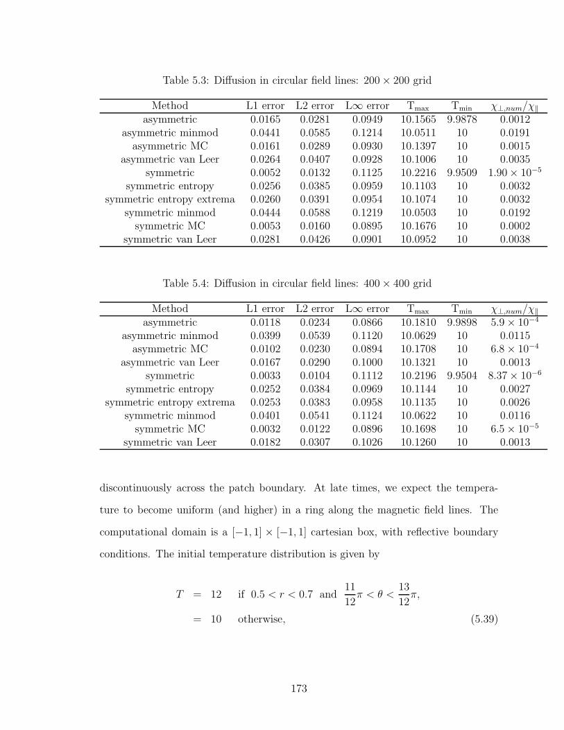
Table 5.3: Diffusion in circular field lines: 200 × 200 grid

Method L1 error L2 error L∞ error Tmax Tmin χ⊥,num/χ‖

asymmetric 0.0165 0.0281 0.0949 10.1565 9.9878 0.0012asymmetric minmod 0.0441 0.0585 0.1214 10.0511 10 0.0191

asymmetric MC 0.0161 0.0289 0.0930 10.1397 10 0.0015asymmetric van Leer 0.0264 0.0407 0.0928 10.1006 10 0.0035

symmetric 0.0052 0.0132 0.1125 10.2216 9.9509 1.90 × 10−5

symmetric entropy 0.0256 0.0385 0.0959 10.1103 10 0.0032symmetric entropy extrema 0.0260 0.0391 0.0954 10.1074 10 0.0032

symmetric minmod 0.0444 0.0588 0.1219 10.0503 10 0.0192symmetric MC 0.0053 0.0160 0.0895 10.1676 10 0.0002

symmetric van Leer 0.0281 0.0426 0.0901 10.0952 10 0.0038

Table 5.4: Diffusion in circular field lines: 400 × 400 grid

Method L1 error L2 error L∞ error Tmax Tmin χ⊥,num/χ‖

asymmetric 0.0118 0.0234 0.0866 10.1810 9.9898 5.9 × 10−4

asymmetric minmod 0.0399 0.0539 0.1120 10.0629 10 0.0115asymmetric MC 0.0102 0.0230 0.0894 10.1708 10 6.8 × 10−4

asymmetric van Leer 0.0167 0.0290 0.1000 10.1321 10 0.0013symmetric 0.0033 0.0104 0.1112 10.2196 9.9504 8.37 × 10−6

symmetric entropy 0.0252 0.0384 0.0969 10.1144 10 0.0027symmetric entropy extrema 0.0253 0.0383 0.0958 10.1135 10 0.0026

symmetric minmod 0.0401 0.0541 0.1124 10.0622 10 0.0116symmetric MC 0.0032 0.0122 0.0896 10.1698 10 6.5 × 10−5

symmetric van Leer 0.0182 0.0307 0.1026 10.1260 10 0.0013

discontinuously across the patch boundary. At late times, we expect the tempera-

ture to become uniform (and higher) in a ring along the magnetic field lines. The

computational domain is a [−1, 1] × [−1, 1] cartesian box, with reflective boundary

conditions. The initial temperature distribution is given by

T = 12 if 0.5 < r < 0.7 and11

12π < θ <

13

12π,

= 10 otherwise, (5.39)

173

where r =√

x2 + y2 and tan θ = y/x. A set of circular field lines centered at the

origin is initialized. The parallel conduction coefficient χ is chosen to be 0.01; there

is no explicit perpendicular diffusion. We evolve the anisotropic conduction equation

(5.3) till time = 200, using different methods that we have discussed. By this time we

expect the temperature to be almost uniform along the circular ring 0.5 < r < 0.7. In

steady state (at late times), energy conservation implies that the the ring temperature

should be 10.1667, while the temperature outside the ring should be maintained at

10.

Figure 5.7 shows the temperature distribution for different methods at time=200.

All methods result in a higher temperature in the annulus r ∈ [0.5, 0.7]. The slope

limited schemes show larger perpendicular diffusion (Tables 5.1-5.4 and Figure 5.10)

compared to the symmetric and asymmetric schemes. The perpendicular numerical

diffusion (χ⊥,num) scales with the parallel diffusion coefficient χ for all methods. How-

ever, for Sovinec’s test problem (discussed in the next subsection) where temperature

is always smooth, and an explicit χ⊥ is present, perpendicular numerical diffusion for

the symmetric method does not scale with χ‖.

The minmod limiter is much more diffusive than van Leer and MC limiters. Both

symmetric and asymmetric methods give a minimum temperature below the initial

minimum of 10, even at late times (see Tables 5.1-5.4). At late times the symmetric

method gives a temperature profile full of non-monotonic oscillations (Figure 5.7).

Although, the slope limited fluxes are more diffusive than the symmetric and asym-

metric methods, they never show undershoots below 10. Although the entropy limited

symmetric method gives temperature undershoots at early times, the minimum tem-

perature is still 10 at late times (see Tables 5.1-5.4 and Figure 5.8). Entropy limiting

combined with a slope limiter at the extrema behaves similar to the slope limiter

based schemes.

Strictly speaking, a hot ring surrounded by a cold background is not a steady

174

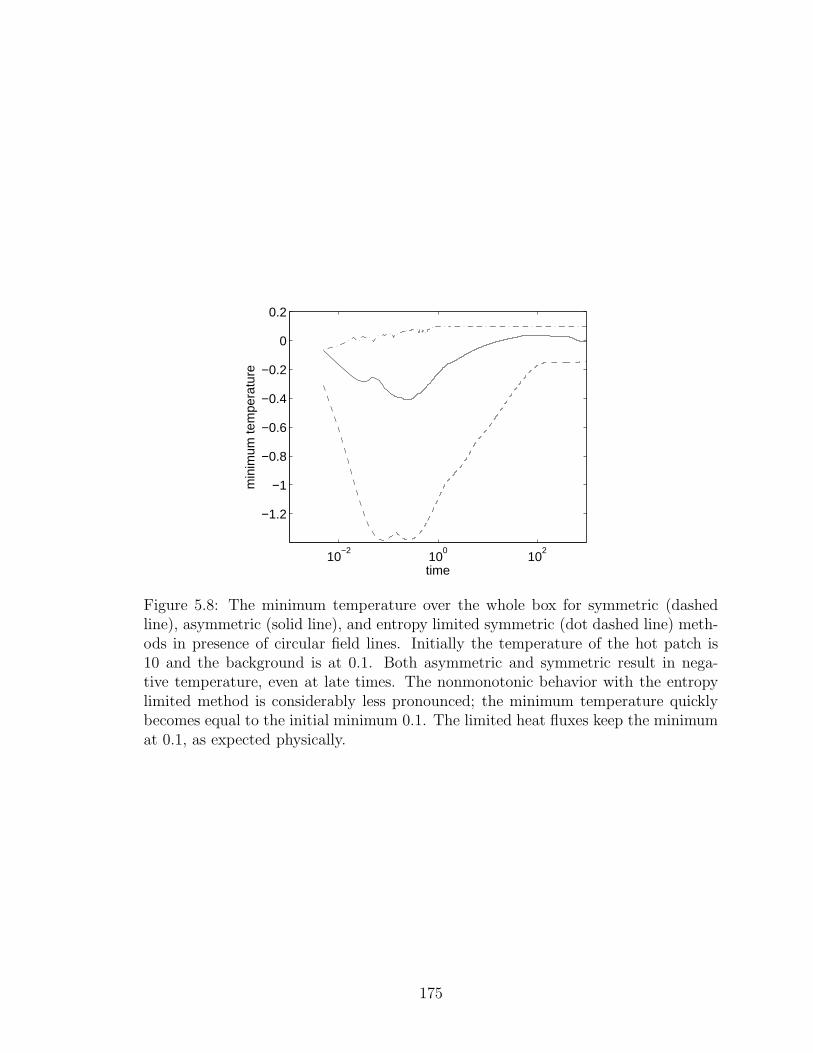
10−2

100

102

−1.2

−1

−0.8

−0.6

−0.4

−0.2

0

0.2

time

min

imum

tem

pera

ture

Figure 5.8: The minimum temperature over the whole box for symmetric (dashedline), asymmetric (solid line), and entropy limited symmetric (dot dashed line) meth-ods in presence of circular field lines. Initially the temperature of the hot patch is10 and the background is at 0.1. Both asymmetric and symmetric result in nega-tive temperature, even at late times. The nonmonotonic behavior with the entropylimited method is considerably less pronounced; the minimum temperature quicklybecomes equal to the initial minimum 0.1. The limited heat fluxes keep the minimumat 0.1, as expected physically.

175

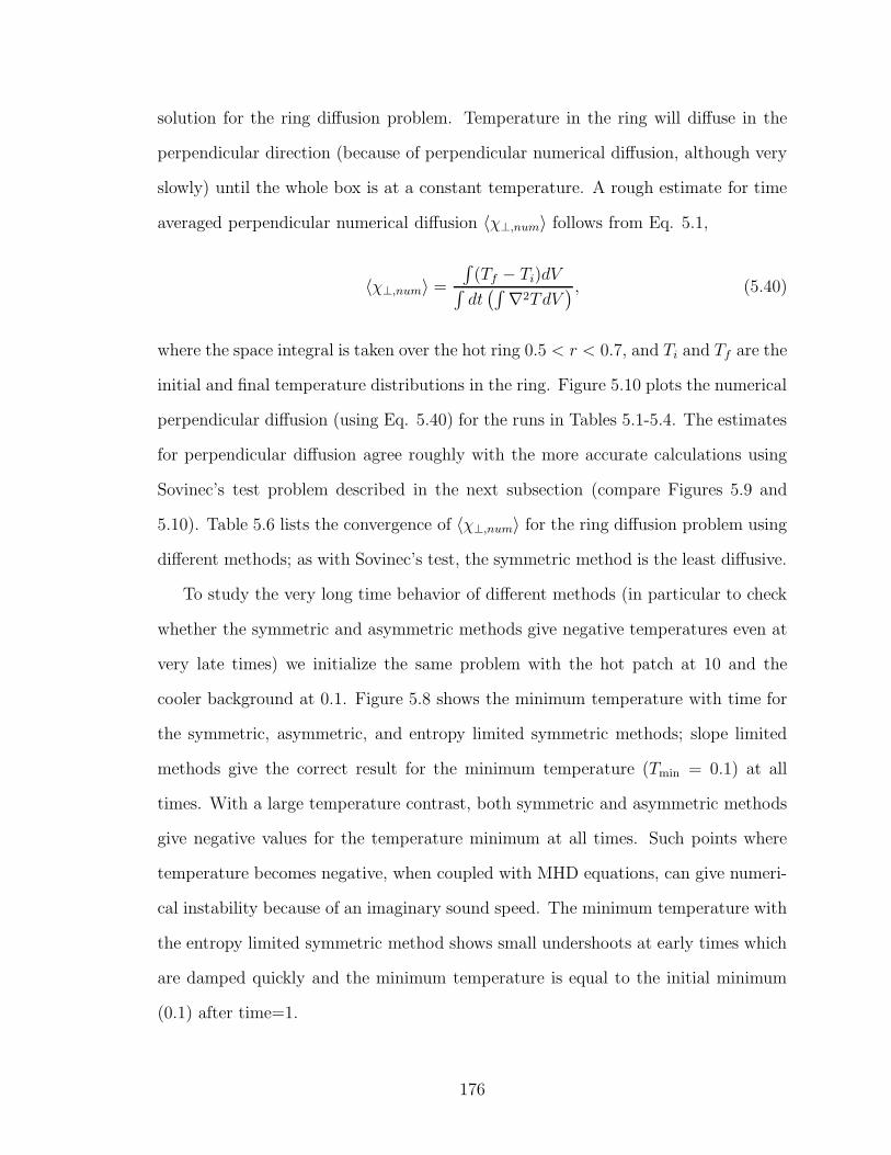
solution for the ring diffusion problem. Temperature in the ring will diffuse in the

perpendicular direction (because of perpendicular numerical diffusion, although very

slowly) until the whole box is at a constant temperature. A rough estimate for time

averaged perpendicular numerical diffusion 〈χ⊥,num〉 follows from Eq. 5.1,

〈χ⊥,num〉 =

∫

(Tf − Ti)dV∫

dt(∫

∇2TdV) , (5.40)

where the space integral is taken over the hot ring 0.5 < r < 0.7, and Ti and Tf are the

initial and final temperature distributions in the ring. Figure 5.10 plots the numerical

perpendicular diffusion (using Eq. 5.40) for the runs in Tables 5.1-5.4. The estimates

for perpendicular diffusion agree roughly with the more accurate calculations using

Sovinec’s test problem described in the next subsection (compare Figures 5.9 and

5.10). Table 5.6 lists the convergence of 〈χ⊥,num〉 for the ring diffusion problem using

different methods; as with Sovinec’s test, the symmetric method is the least diffusive.

To study the very long time behavior of different methods (in particular to check

whether the symmetric and asymmetric methods give negative temperatures even at

very late times) we initialize the same problem with the hot patch at 10 and the

cooler background at 0.1. Figure 5.8 shows the minimum temperature with time for

the symmetric, asymmetric, and entropy limited symmetric methods; slope limited

methods give the correct result for the minimum temperature (Tmin = 0.1) at all

times. With a large temperature contrast, both symmetric and asymmetric methods

give negative values for the temperature minimum at all times. Such points where

temperature becomes negative, when coupled with MHD equations, can give numeri-

cal instability because of an imaginary sound speed. The minimum temperature with

the entropy limited symmetric method shows small undershoots at early times which

are damped quickly and the minimum temperature is equal to the initial minimum

(0.1) after time=1.

176

5.7.2 Convergence studies: measuring χ⊥,num

We have use the steady state test problem described in [181] to measure the perpen-

dicular numerical diffusion coefficient, χ⊥. The computational domain is a unit square

[−0.5, 0.5] × [−0.5, 0.5], with vanishing temperature at the boundaries. The source

term Q = 2π2 cos(πx) cos(πy) that drives the lowest eigenmode of the temperature

distribution is added to the anisotropic diffusion equation, Eq. 5.1; the anisotropic

diffusion equation with a source term possesses a steady state solution. The equation

that we evolve is

∂e

∂t= −∇ · q +Q; (5.41)

a forward in time centered in space (FTCS) differencing is used to add the source

term.

The magnetic field is derived from the flux function of the form ψ ∼ cos(πx) cos(πy);

this results in circular field lines centered at the origin. The temperature eigenmode

driven by the source function Q is constant along the field lines. The steady state

solution for the temperature is T (x, y) = χ−1⊥ cos(πx) cos(πy), independent of χ‖. The

perpendicular diffusion coefficient, χ⊥, is chosen to be unity, and T−1(0, 0) provides

a measure of total perpendicular diffusion, the sum of χ⊥ (the explicit perpendicular

diffusion) and χ⊥,num (the perpendicular numerical diffusion).

Figure 5.9 shows the perpendicular numerical diffusivity χ⊥,num = |T−1(0, 0) −

T−1iso (0, 0)| for χ‖/χ⊥ = 10, 100 using different methods (where T−1

iso (0, 0) is the tem-

perature at the origin when χ‖ = χ⊥ is used for the same resolution). Gunter et al.

[76] and Sovinec et al. [181] use χ⊥,num = |T−1(0, 0) − 1| to measure perpendicular

numerical diffusion; this is not precise and exaggerates the error for the symmetric

method.

The perpendicular perpendicular diffusion (χ⊥,num) for all methods except the

symmetric method increases linearly with χ‖/χ⊥. This property has been emphasized

177

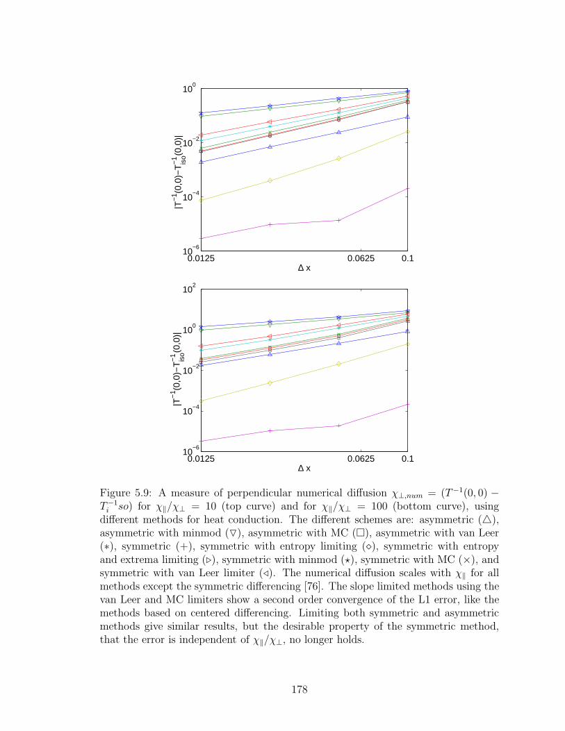
0.10.0125 0.062510

−6

10−4

10−2

100

∆ x

|T−

1 (0,0

)−T

iso

−1(0

,0)|

0.10.0125 0.062510

−6

10−4

10−2

100

102

∆ x

|T−

1 (0,0

)−T

iso

−1(0

,0)|

Figure 5.9: A measure of perpendicular numerical diffusion χ⊥,num = (T−1(0, 0) −T−1

i so) for χ‖/χ⊥ = 10 (top curve) and for χ‖/χ⊥ = 100 (bottom curve), usingdifferent methods for heat conduction. The different schemes are: asymmetric (),asymmetric with minmod (), asymmetric with MC (), asymmetric with van Leer(∗), symmetric (+), symmetric with entropy limiting (⋄), symmetric with entropyand extrema limiting (⊲), symmetric with minmod (⋆), symmetric with MC (×), andsymmetric with van Leer limiter (⊳). The numerical diffusion scales with χ‖ for allmethods except the symmetric differencing [76]. The slope limited methods using thevan Leer and MC limiters show a second order convergence of the L1 error, like themethods based on centered differencing. Limiting both symmetric and asymmetricmethods give similar results, but the desirable property of the symmetric method,that the error is independent of χ‖/χ⊥, no longer holds.

178

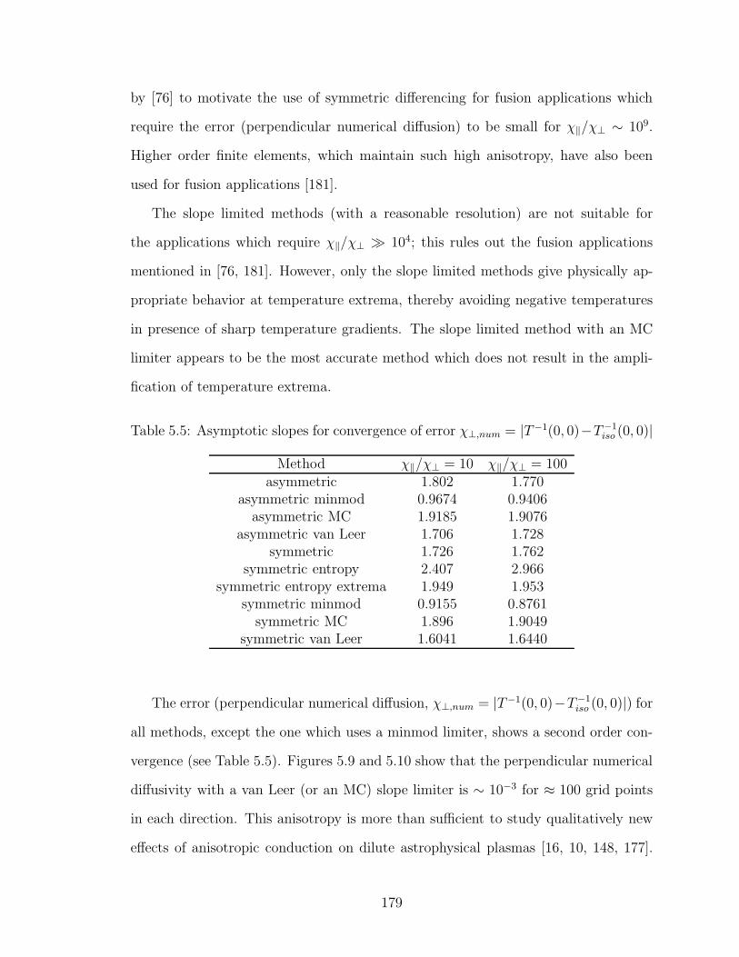
by [76] to motivate the use of symmetric differencing for fusion applications which

require the error (perpendicular numerical diffusion) to be small for χ‖/χ⊥ ∼ 109.

Higher order finite elements, which maintain such high anisotropy, have also been

used for fusion applications [181].

The slope limited methods (with a reasonable resolution) are not suitable for

the applications which require χ‖/χ⊥ ≫ 104; this rules out the fusion applications

mentioned in [76, 181]. However, only the slope limited methods give physically ap-

propriate behavior at temperature extrema, thereby avoiding negative temperatures

in presence of sharp temperature gradients. The slope limited method with an MC

limiter appears to be the most accurate method which does not result in the ampli-

fication of temperature extrema.

Table 5.5: Asymptotic slopes for convergence of error χ⊥,num = |T−1(0, 0)−T−1iso (0, 0)|

Method χ‖/χ⊥ = 10 χ‖/χ⊥ = 100asymmetric 1.802 1.770

asymmetric minmod 0.9674 0.9406asymmetric MC 1.9185 1.9076

asymmetric van Leer 1.706 1.728symmetric 1.726 1.762

symmetric entropy 2.407 2.966symmetric entropy extrema 1.949 1.953

symmetric minmod 0.9155 0.8761symmetric MC 1.896 1.9049

symmetric van Leer 1.6041 1.6440

The error (perpendicular numerical diffusion, χ⊥,num = |T−1(0, 0)−T−1iso (0, 0)|) for

all methods, except the one which uses a minmod limiter, shows a second order con-

vergence (see Table 5.5). Figures 5.9 and 5.10 show that the perpendicular numerical

diffusivity with a van Leer (or an MC) slope limiter is ∼ 10−3 for ≈ 100 grid points

in each direction. This anisotropy is more than sufficient to study qualitatively new

effects of anisotropic conduction on dilute astrophysical plasmas [16, 10, 148, 177].

179

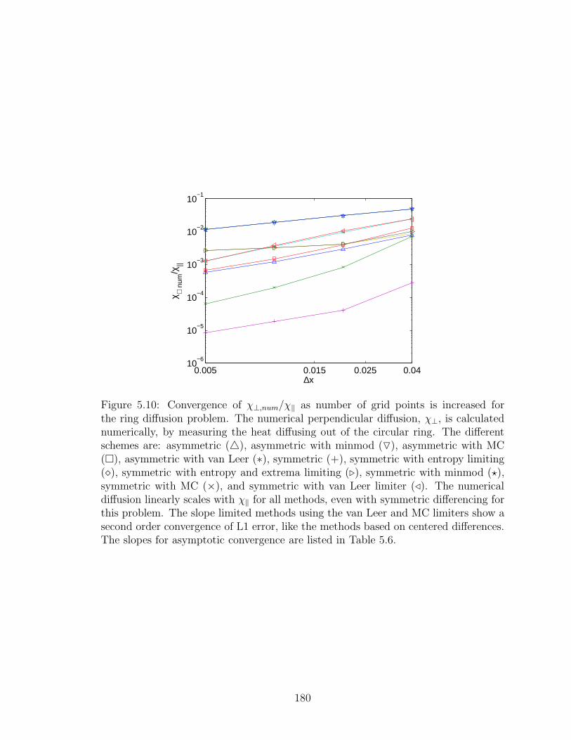
0.005 0.015 0.025 0.0410

−6

10−5

10−4

10−3

10−2

10−1

∆x

χ ⊥ nu

m/χ

||

Figure 5.10: Convergence of χ⊥,num/χ‖ as number of grid points is increased forthe ring diffusion problem. The numerical perpendicular diffusion, χ⊥, is calculatednumerically, by measuring the heat diffusing out of the circular ring. The differentschemes are: asymmetric (), asymmetric with minmod (), asymmetric with MC(), asymmetric with van Leer (∗), symmetric (+), symmetric with entropy limiting(⋄), symmetric with entropy and extrema limiting (⊲), symmetric with minmod (⋆),symmetric with MC (×), and symmetric with van Leer limiter (⊳). The numericaldiffusion linearly scales with χ‖ for all methods, even with symmetric differencing forthis problem. The slope limited methods using the van Leer and MC limiters show asecond order convergence of L1 error, like the methods based on centered differences.The slopes for asymptotic convergence are listed in Table 5.6.

180

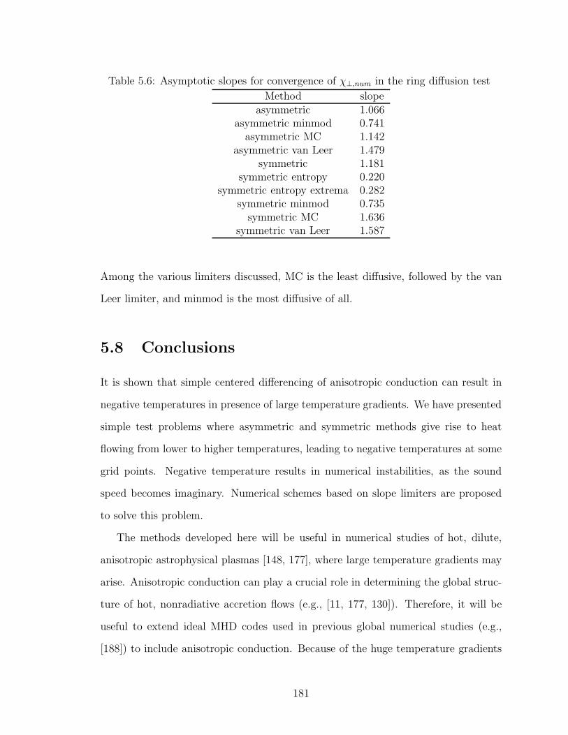
Table 5.6: Asymptotic slopes for convergence of χ⊥,num in the ring diffusion test

Method slopeasymmetric 1.066

asymmetric minmod 0.741asymmetric MC 1.142

asymmetric van Leer 1.479symmetric 1.181

symmetric entropy 0.220symmetric entropy extrema 0.282

symmetric minmod 0.735symmetric MC 1.636

symmetric van Leer 1.587

Among the various limiters discussed, MC is the least diffusive, followed by the van

Leer limiter, and minmod is the most diffusive of all.

5.8 Conclusions

It is shown that simple centered differencing of anisotropic conduction can result in

negative temperatures in presence of large temperature gradients. We have presented

simple test problems where asymmetric and symmetric methods give rise to heat

flowing from lower to higher temperatures, leading to negative temperatures at some

grid points. Negative temperature results in numerical instabilities, as the sound

speed becomes imaginary. Numerical schemes based on slope limiters are proposed

to solve this problem.

The methods developed here will be useful in numerical studies of hot, dilute,

anisotropic astrophysical plasmas [148, 177], where large temperature gradients may

arise. Anisotropic conduction can play a crucial role in determining the global struc-

ture of hot, nonradiative accretion flows (e.g., [11, 177, 130]). Therefore, it will be

useful to extend ideal MHD codes used in previous global numerical studies (e.g.,

[188]) to include anisotropic conduction. Because of the huge temperature gradients

181

that may occur in global disk simulations with a hot, dilute corona and a cold, dense

disk, slope limited methods, which guarantee the positivity of temperature, must be

used.

Although the slope and entropy limited methods in the present form are not suit-

able for fusion applications that require accurate resolution of perpendicular diffusion

for huge anisotropy (χ‖/χ⊥ ∼ 109), they are appropriate for astrophysical applications

with large temperature gradients. A relatively small anisotropy of thermal conduction

is sufficient to study the effects of anisotropic conduction. The primary advantage of

the limited methods is their robustness in presence of large temperature gradients.

Apart from the simulations of dilute astrophysical plasmas with large temperature

gradients (e.g., solar corona, magnetosphere, and magnetized collisionless shocks),

our methods may find a use in diverse fields where anisotropic diffusion is important,

e.g., image processing, biological transport, and geological systems.

Chapters 3 and 4 explored local (linear and nonlinear) properties of the MRI in the

collisionless regime, but global calculations are required to study the relative roles of

conduction, convection, and outflows, which determine the radial profile of different

quantities, e.g., density, temperature, and radiation. Anisotropic conduction (and

pressure) is crucial to understand the structure of hot, thick, collisionless RIAFs (see

Section 1.4), and the slope limited methods are the only option for robust nonlinear

simulations because large temperature gradients (e.g., the disk corona interface) arise

naturally in global disk simulations.

182

Chapter 6

Conclusions

The main goal of the thesis was to study plasma kinetic processes operating in radia-

tively inefficient accretion flows (RIAFs) around compact objects, such as the super-

massive black hole in the Galactic center and other nearby galactic centers (see 1.4 for

details). Global MHD simulations of hot, thick accretion disks show that very little

of the gas initially accreted from the outer regions actually makes it to the last stable

orbit; most of the matter is lost as magnetized outflows [188, 84, 83, 95, 149, 155].

Although the reduction of the net mass accretion rate is part of the reason for the

low luminosity, it is required by most models that the electrons radiate much less

efficiently than the standard 10% efficiency for such low observed luminosities ([156],

see 1.4). Some models, e.g., ADAFs, ascribe the low luminosity to low electron tem-

perature compared to ions. To understand whether electrons can be maintained much

cooler than ions, one needs to understand the conversion of gravitational energy into

internal energy of electrons and ions.

We began by looking into the MRI in the collisionless regime and studied the tran-

sition from collisionless to collisional regimes as the collision frequency is increased

(see Chapter 3). We show the equivalence of the drift kinetic equation and its mo-

ments closed with a Landau fluid closure for parallel heat flux, in both collisional

183

and collisionless regimes. Unlike MHD, where energy is dissipated (resistively and

viscously) only at small scales, the collisionless plasmas have damped modes at all

scales which can heat electrons and ions differently (see Figure 3.4). The linear stud-

ies were followed by 3-D local unstratified shearing box simulations of magnetized

collisionless plasmas, using the kinetic MHD (KMHD) formalism closed with a local

form of Landau fluid closure for parallel heat flux (see Chapter 4). Although, both

linear studies and nonlinear simulations were carried out in a one fluid plasma with

Ti ≫ Te, we can roughly estimate the heating rate for both electrons and ions. It is

important to investigate what collisionless effects can do to the structure of RIAFs;

especially to consider anisotropic thermal conduction, since it has important implica-

tions for the convective stability of plasmas [10, 11]. While implementing anisotropic

conduction we discovered that the centered finite differencing of anisotropic conduc-

tion can give negative temperature in regions with large temperature gradients. To

tackle this problem we developed a method where the transverse temperature gradi-

ent is obtained, not by simple averaging, but by using slope limiters. The method

based on slope limiters guarantees the positivity of temperature (see Chapter 5).

6.1 Summary

To assess the importance of plasma kinetic effects in RIAFs we began with the study of

collisionless MRI in the linear regime. The effect of collisions was introduced through

a BGK collision operator. We use 3+1 Landau fluid closure for parallel thermal fluxes,

which is equivalent to a Pade approximation for the fully kinetic plasma response.

The Landau closure gives a good approximation to linear collisionless effects like

Landau/Barnes damping.

We verify the equivalence of a fully kinetic analysis and the one based on Landau

closure by considering the modes of a magnetized Keplerian disk, in both high and

184

low collisionality regimes. Heating in a collisionless disk can occur at all scales due

to Landau/Barnes damping of the fast and slow modes; whereas, in MHD resistive

and viscous heating at small scales is the only source of heating. Since collisionless

damping is a resonant phenomenon, it can heat electrons or ions preferentially (Tp ≫

Te is required by some RIAF models; see 1.4). The fastest growing MRI is twice

as fast in the collisionless regime as compared to MHD. More importantly, it occurs

at much larger length scales compared to MHD. Fast growth at large scales can in

principle result in a different nonlinear saturation (for magnetic energy and stress)

compared to MHD (though our nonlinear simulations to date find that in practice

the final nonlinear spectra are similar). The MRI transitions from the collisionless

to the Braginskii regime (when the mean free path becomes short compared to the

wavelength, ν & Ω√β), and then to the MHD regime (when the parallel viscous

damping becomes negligible, ν & Ωβ), as the collision frequency is increased.

Balbus and Islam (see [12, 96]) have studied collisionless effects on the MRI by

adding Braginskii anisotropic stress to the MHD equations, and verified our results;

they emphasize the importance of anisotropic stress and call it the “magnetoviscous”

instability because the instability occurs at long wavelengths even for an arbitrarily

small field strength.

The linear studies were followed by local shearing box simulations of magnetized

collisionless disks. The ZEUS MHD code was modified to include the kinetic MHD

terms: anisotropic pressure in the equation of motion, and equations evolving p‖

and p⊥ closed by a local Landau fluid closure for heat flux along the field lines.

Adiabatic invariant (µ = p⊥/B) is conserved for collisionless plasmas at length scales

much larger than the Larmor radius and time scales much larger than the gyroperiod.

Pressure anisotropy (p⊥ > p‖) is created naturally as magnetic field is amplified by the

MRI. Small scale instabilities—mirrror, ion-cyclotron, and firehose—are excited even

at at small pressure anisotropies (∆p/p & few/β). Although, mirror and firehose

185

instabilites are correctly captured in Landau MHD, we have to include a subgrid

model for pressure isotropization due to these and ion-cyclotron instabilities because

at large pressure anisotropies the fastest growing instabilities occur at the gyroradius

scale and violate adiabatic invariance.

The result of pressure anisotropy is that there is a qualitatively new mechanism

to transport angular momentum, the anisotropic stress. Apart from appearing in the

equation of motion, anisotropic stress also appears in the internal energy equation,

resulting in heating. The anisotropic stress is as important as the Maxwell stress,

and depends only weakly on kL (the parameter in the local Landau heat fluxes) and

the pitch angle scattering model.

Pitch angle scattering due to microinstabilities limit the pressure anisotropy and

results in MHD-like behavior—the reason MHD often provides a good approximation

for large scale dynamics of astrophysical systems. What MHD does not tell us is how

the energy released from accretion is dissipated—whether it goes into electrons or

ions? A fully kinetic simulation with huge resolution can address the issue of plasma

heating; but insights can be gained from fluid treatments like kinetic MHD (e.g.,

anisotropic stress can heat both electrons and ions).

The kinetic MHD simulations also show that the kinetic and magnetic energies are

peaked at large scales (as in MHD). The simulations with Bφ = Bz initially, confirm

that the linear growth rate in the kinetic regime is twice faster than in MHD; but

the nonlinear saturation is not very different in the two regimes. In fact, somewhat

counter-intuitively, the saturated magnetic energy for Bφ = Bz simulations is smaller

compared to simulations with only a vertical field with the same β. Anisotropic stress

can be larger than the Maxwell stress for β > a few 100. To sum up, the nonlinear

saturation of the MRI is quite similar for MHD and kinetic regimes.

Along with the local studies, it is crucial to understand the global structure of hot

collisionless accretion flows. Global MHD simulations have shown that very little of

186

the mass initially accreted from the outer regions actually accreted on to the black

hole; most of it is lost in outflows. Anisotropic thermal conduction can be crucial

for the structure of hot collisionless accretion flows; collisionless plasmas with long

mean free path can transport heat very efficiently along the field lines. When we

used finite differencing to implement anisotropic conduction in a global simulation,

we discovered that the temperature became negative at the torus-corona interface.

This led us to investigate numerical algorithms for anisotropic thermal conduction

in presence of large temperature gradients. We devised simple test problems that

demonstrated that existing algorithms (both symmetric and asymmetric differencing)

can result in heat flux out of a cold region, causing temperature to become negative

in regions with high temperature gradient. This problem was solved by using slope

limiters to obtain the transverse temperature gradient, instead of using a simple

arithmetic average. The limiter-based methods are slightly more diffusive across

field lines than the asymmetric method, but still show second order convergence.

Although the symmetric method has very small numerical diffusion, it gives rise

to high frequency non-monotonic temperature fluctuations with large temperature

gradients.

6.2 Future directions

There are several directions for future work, for both local and global studies. Till

now we have only done single fluid simulations, assuming the electrons to be cold.

We can extended these simulations to include electrons to study comparative heating

of electrons and ions. The original ZEUS code did not conserve energy (up to 90%

of energy released from accretion was lost numerically), but energy conservation can

be restored to a large extent by adding the energy lost while updating velocities

and magnetic fields into heating of the plasma [194], or by switching to codes using

187

conservative algorithms (such as the recently developed ATHENA code [65]). In the

absence of explicit resistivity and viscosity, the sources in the internal energy equation

are: energy lost in updating magnetic fields (mimics magnetic dissipation), energy

lost when updating velocity (represents viscous losses), the −p∇ · V heating, and the

work done by anisotropic stress.

The energy-conserving one fluid simulations show that the work done by anisotropic

stress is comparable to (or even larger than) the energy lost in magnetic field or

velocity update; this means that the physical anisotropic heating is not negligible

compared to resistive or viscous heating. This has important implications for local

two-fluid simulations. The electron pressure will also be anisotropic (T⊥,e > T‖,e)

because of adiabatic invariance, and the anisotropy will be limited by pitch angle

scattering due to electron whistler instability with ∆p/p ∼ (a few)/β (see [99, 68]).

This means that the heating rate due to anisotropic stress, (1/e)de/dt, is comparable

for electrons and ions, and is comparable to resistive or viscous heating. Thus, local

two-fluid simulations which conserve energy can shed some light on electron/ion heat-

ing and whether Tp/Te ≫ 1 is possible. This approach where both electrons and ions

are heated because of the energy released from accretion is different from an approach

where one looks for collisionless heat transport from hot ions to cold electrons (e.g.,

[24]).

Another area of progress is to implement more accurate non-local closures for

thermal conduction in nonlinear simulations (see Chapter 2); till now we have used a

crude, local approximation with a parameter kL that exaggerates damping for scales

smaller than 2π/kL and reduces damping for larger scales. A local approximation may

be fine if pitch-angle scattering due to microinstabilities reduces the effective mean free

path to be comparable to the fastest growing MRI mode, which reduces the sensitivity

to the parameter kL. However, pitch angle scattering due to microinstabilities is not

uniform. This intermittency may lead to a larger effective mean free path than simple

188

estimates at first suggest. It is important to understand the role of intermittent

scattering structures in imposing MHD-like dynamics in collisionless plasmas.

It’s important to realize that astrophysical plasmas are very different from fusion

plasmas; magnetic fields are strong in fusion devices, with only small perturbation

from the equilibrium condition, but in astrophysical plasmas with subthermal fields,

strong shear flows can mix the fields and magnetic fields can be chaotic. Chaotic

fields reduce thermal conduction as the effective mean free path is reduced to the

field correlation length [43], this may mean that results do not sensitively depend on

thermal conduction.

Another approach, which is computationally more challenging but feasible for

some problems, is to evolve the drift kinetic equation (DKE, Eq. 2.7) to evolve the

distribution function in a 5-D phase space and to use its moments for p‖ and p⊥ to

close the kinetic MHD moment hierarchy. Many hydrodynamic codes are based on

Riemann solvers; given a discontinuity at grid boundaries, Riemann solvers divide the

discontinuity into wave families of the system and give the evolution of the variables

due to flux through the boundaries [116]. The number of modes of the drift kinetic

equation is huge, and it is impossible to solve the Riemann problem exactly. One

approach to solve hyperbolic equations that does not require the solution of Riemann

problems is based on central methods (alternatively, they can be related to a simple,

approximate Riemann solver; see [143, 112]); central methods have also been applied

to MHD simulations [9]. The DKE simulations do not require the closure approx-

imation, but like in KMHD with Landau closures, subgrid models for pitch angle

scattering to microinstabilities will be required. It is also possible to carry out full

Vlasov or particle-in-cell (PIC) simulations where a subgrid model for microinstabil-

ities is not required, but for such simulations to be applicable to RIAFs they will

need to resolve both the large MRI scale and the Larmor radius scale (8 orders of

magnitudes smaller than the disk height scale).

189

Recent global MHD simulations were responsible for understanding that only a

small fraction of gas accreted in outer region actually make it to the black hole, most

of it is lost in outflows. A small accretion rate is one reason for small radiative lu-

minosities of RIAFs. An important direction for future research is to include kinetic

MHD effects like anisotropic conduction in global simulations. Since plasma in RIAFs

is hot and collisionless, anisotropic thermal conduction is rapid. This can be impor-

tant in determining the structure of RIAFs. The structure of the self-similar solution

for a RIAF changes dramatically if a saturated form of thermal conduction (due to

free streaming of particles) is included [130]. Another reason that anisotropic con-

duction can be important is because the convective stability criterion for anisotropic

plasmas is that temperature decreases outwards, dT/dr < 0, instead of the usual

Schwarzschild condition of entropy increasing outwards, ds/dr < 0 [16, 10]. The

effect of thermal conduction is subtle because the MRI may generate chaotic fields

and suppress thermal conduction and impose more MHD-like behavior, instead of

giving a state which is stable to the magnetothermal instability. Thus, it will impor-

tant to know whether anisotropic thermal conduction will be a small effect due to its

suppression because of MHD turbulence, or it will alter the structure of RIAFs.

190

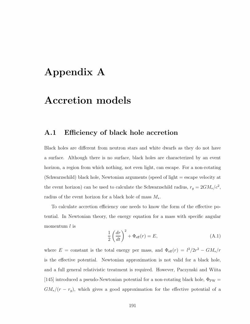
Appendix A

Accretion models

A.1 Efficiency of black hole accretion

Black holes are different from neutron stars and white dwarfs as they do not have

a surface. Although there is no surface, black holes are characterized by an event

horizon, a region from which nothing, not even light, can escape. For a non-rotating

(Schwarzschild) black hole, Newtonian arguments (speed of light = escape velocity at

the event horizon) can be used to calculate the Schwarzschild radius, rg = 2GM∗/c2,

radius of the event horizon for a black hole of mass M∗.

To calculate accretion efficiency one needs to know the form of the effective po-

tential. In Newtonian theory, the energy equation for a mass with specific angular

momentum l is

1

2

(

dr

dt

)2

+ Φeff(r) = E, (A.1)

where E = constant is the total energy per mass, and Φeff(r) = l2/2r2 − GM∗/r

is the effective potential. Newtonian approximation is not valid for a black hole,

and a full general relativistic treatment is required. However, Paczynski and Wiita

[145] introduced a pseudo-Newtonian potential for a non-rotating black hole, ΦPW =

GM∗/(r − rg), which gives a good approximation for the effective potential of a

191

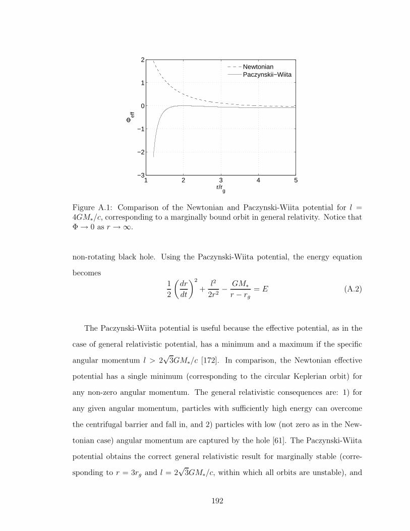
1 2 3 4 5−3

−2

−1

0

1

2

r/rg

Φef

f

NewtonianPaczynskii−Wiita

Figure A.1: Comparison of the Newtonian and Paczynski-Wiita potential for l =4GM∗/c, corresponding to a marginally bound orbit in general relativity. Notice thatΦ → 0 as r → ∞.

non-rotating black hole. Using the Paczynski-Wiita potential, the energy equation

becomes

1

2

(

dr

dt

)2

+l2

2r2− GM∗

r − rg

= E (A.2)

The Paczynski-Wiita potential is useful because the effective potential, as in the

case of general relativistic potential, has a minimum and a maximum if the specific

angular momentum l > 2√

3GM∗/c [172]. In comparison, the Newtonian effective

potential has a single minimum (corresponding to the circular Keplerian orbit) for

any non-zero angular momentum. The general relativistic consequences are: 1) for

any given angular momentum, particles with sufficiently high energy can overcome

the centrifugal barrier and fall in, and 2) particles with low (not zero as in the New-

tonian case) angular momentum are captured by the hole [61]. The Paczynski-Wiita

potential obtains the correct general relativistic result for marginally stable (corre-

sponding to r = 3rg and l = 2√

3GM∗/c, within which all orbits are unstable), and

192

the marginally bound orbit (with r = 2rg and l = 4GM∗/c, particles with E > 0 can

fall directly on to the hole for specific angular momentum smaller than this). Figure

A.1 shows the Newtonian, and the Paczynski-Wiita potential for a marginally bound

orbit, with l = 4GM∗/c.

The presence of a last stable orbit has important consequences for accretion effi-

ciency; beyond this, matter plunges in the black hole with no time to radiate. Thus,

for a Schwarzschild black hole, matter radiates half the released gravitational energy

(and retains the other half as the kinetic energy) till the last stable orbit (3rg). This

gives a radiative efficiency of η = (GM∗/6rg)/c2 = 1/12. The relativistic relativistic

result of 6% is not too far off. For a rotating Kerr hole the last stable orbit moves

further in, resulting in a larger efficiency; a maximally rotating black hole has an

efficiency of 42.3% (see [133] for detailed introduction to spinning black holes).

A.2 Bondi accretion

Bondi accretion [35], a model for steady, spherical accretion of matter with vanishing

angular momentum (e.g., a star accreting from a stationary gas cloud), is commonly

used to estimate the accretion rate M from the measurement of ambient density and

temperature. The following presentation is based on [61].

We will solve the spherically symmetric, hydrodynamic equations in steady state

using spherical polar coordinates (r, θ, φ) with origin at the center of the star. The

fluid variables are independent of θ and φ, and the gas has only a radial velocity

component Vr = V . The equation of continuity

1

r2

d

dr

(

r2ρV)

= 0, (A.3)

gives a constant inward flux of matter M = −4πr2ρV = constant; for accretion

193

Figure A.2: Mach number (the ratio of fluid velocity and sound speed) as a functionof radius for spherical accretion with different inner and outer boundary conditions.Solution V I corresponds to accretion and V to a spherical wind. Taken from AlanHood’s lecture notes, http://www-solar.mcs.st-and.ac.uk/˜alan/sun course/.

V < 0, as matter falls in. The Euler equation becomes

VdV

dr+

1

ρ

dp

dr+GM∗

r2= 0. (A.4)

A polytropic equation of state is used, p = Kργ , with 1 < γ < 5/3.

Using dP/dr = a2dρ/dr, where a =√

γp/ρ is the sound speed, the continuity and

Euler equations can be combined to give

1

2

(

1 − a2

V 2

)

d

drV 2 = −GM∗

r2

[

1 −(

2a2r

GM∗

)]

. (A.5)

This form is useful to draw inferences about steady, spherically symmetric accretion.

At large distances (r ≫ GM∗/2a2), the right side of Eq. A.5 is positive, and dV 2/dr <

0 at large distances where gas is expected to be at rest. This implies that the gas is

subsonic (V 2 < a2) for r ≫ GM∗/2a2; this is reasonable because far from the star, the

194

gas has a non-zero temperature. One need to specify the inner boundary condition in

addition to the outer (ambient) boundary conditions to uniquely specify the solution;

we choose V 2 > a2 for small r for accretion (see Figure A.2).

At a radius ra = GM∗/2a2, either V 2 = a2 or d/dr(V 2) = 0; latter is true for

accretion solution with a supersonic flow for r < ra. The sonic point condition,

ra = GM∗/2a2 leads to the relation between the accretion rate M and the ambient

conditions. The integral form of Eq. A.4 is the Bernoulli integral:

V 2

2+

a2

γ − 1− GM

r= Be, a constant. (A.6)

The boundary condition at r → ∞, and the sonic point condition a2(ra) = GM∗/2ra

combine to give a(ra) = a(∞)√

2/(5 − 3γ), which leads to the constant accretion

rate in terms of sonic point variables, M = 4πr2aρ(ra)a(ra). Since a ∝ ργ−1,

ρ(ra) = ρ(∞)

[

a(ra)

a(∞)

]2/(γ−1)

; (A.7)

this combined with M in terms of sonic point variables gives the required expression

for M in terms of conditions at infinity:

M = πG2M2∗

ρ(∞)

a3(∞)

[

2

5 − 3γ

](5−3γ)/2(γ−1)

. (A.8)

The dependence of M on γ is weak. For γ = 1.4, Eq. A.8 gives

M ∼= 1.4 × 1011

(

M

M⊙

)(

ρ(∞)

10−24 g cm−3

)(

a(∞)

10 km s−1

)−3

g s−1. (A.9)

For r ≪ ra, matter falls freely, v2 ∼= 2GM∗/r; the continuity equation gives

ρ ∼= ρ(ra)(ra/r)3/2 for r < ra. One can define an effective accretion radius, beyond

which the thermal energy of the gas is larger than the gravitational binding energy.

195

The ratio of the thermal and gravitational binding energy is (ma2(r)/2)/(GM∗m/r) ∼

r/racc, for r & racc, since a(r) ∼ a(∞) for r > racc ≡ 2GM∗/a2(∞) [61]. Hence,

for r ≫ racc the gravitational pull of the star has negligible effect on the gas. In

terms of the Bondi radius, an approximation for the mass accretion rate is given by

M ∼ πr2acca(∞)ρ(∞).

196

Appendix B

Linear closure for high and low

collisionality

B.1 Closure for high collisionality: |ζ| ≫ 1

For |ζ | ≫ 1, Z (ζ) ≈ −1/ζ − 1/2ζ3 − 3/4ζ5, R ≈ −1/2ζ2 − 3/4ζ4, 1 + 2ζ2R ≈

−3/2ζ2 − 15/4ζ4, Z − 2ζR ≈ 1/ζ3 + 3/ζ5. Equation (3.26) then becomes

δn

n0

− δp⊥p0

= −δBB0

(

1 +1

2ζ2

)

− ζ2ζ

(

1 +1

2ζ2

)(

δT

T0

− δB

B0

)

. (B.1)

Assuming |ζ1/ζ2| ≪ 1 (a high collisionality limit ω ≪ ν) and using the binomial

expansion we get

δn

n0− δp⊥

p0= −

1 − ζ1ζ2

+1

ζ22

(

1

2+ ζ2

1

)

− ζ1ζ32

(

1

2+ ζ2

1

)(

ζ1ζ2

δB

B0+δT

T0

)

. (B.2)

To the lowest nonvanishing order one gets

δn

n0

ζ1ζ2

− δp⊥p0

(

1

3+

2

3

ζ1ζ2

)

+δp‖p0

(

1

3− ζ1

3ζ2

)

= −ζ1ζ2

δB

B0. (B.3)

197

Expanding equation (3.27) gives

−δnn0

(

3

2ζ2+

15

4ζ4

)

+δp‖p0

(

1

2ζ2+

3

4ζ4

)

= −δBB0

(

1

ζ2+

3

ζ4

)

+

(

δB

B0

− δn

n0

+δT

2T0

)

ζ2

(

1

ζ3+

3

ζ5

)

. (B.4)

Again using the binomial expansion for |ζ1/ζ2| ≪ 1 we get

δn

n0

(

−3

2

ζ1ζ2

+9

2

(

ζ1ζ2

)2

+3

4ζ22

)

+δp‖p0

(

1

3− 1

2

ζ1ζ2

+1

2

(

ζ1ζ2

)2

+1

4ζ22

)

+δp⊥p0

(

−1

3+ζ1ζ2

− 2

(

ζ1ζ2

)2

− 1

ζ22

)

=δB

B0

(

−ζ1ζ2

+ 3

(

ζ1ζ2

)2)

. (B.5)

The lowest order solution is

−3ζ12ζ2

δn

n0+

(

1

3− ζ1

2ζ2

)

δp‖p0

+

(

−1

3+ζ1ζ2

)

δp⊥p0

= −ζ1ζ2

δB

B0. (B.6)

We shall expand the parallel and perpendicular pressure perturbations as δp⊥ =

δ0p⊥ + ζ1/ζ2δ1p⊥ + (ζ1/ζ2)

2δ2p⊥ + ... and δp‖ = δ0p‖ + ζ1/ζ2δ1p‖ + (ζ1/ζ2)

2δ2p‖ + ...

From equations (B.2) and (B.5) one gets δ0p‖/p0 = δ0p⊥/p0 = 5δn/3n0 for the lowest

order, and (δp⊥ − δ1p‖)/p0 = 3δB/B0 − 2δn/n0. To the next order we can expand

the solution as

δp‖p0

=5δn

3n0

+ζ1ζ2

δ1p‖p0

+

(

ζ1ζ2

)2 δ2p‖p0

, (B.7)

δp⊥p0

=5δn

3n0+ζ1ζ2

(

δ1p‖p0

+ 3δB

B0− 2

δn

n0

)

+

(

ζ1ζ2

)2δ2p⊥p0

. (B.8)

To the next order in ζ1/ζ2 in equation (B.2) one gets

− 1

2ζ21

δn

n0

+1

2

δ1p‖p0

+1

3

(

δ2p‖p0

− δ2p⊥p0

)

= 0. (B.9)

198

To the next order in equation (B.5) we get

(

2 +1

3ζ21

)

δn

n0− δ1p‖

p0+

1

3

(

δ2p‖p0

− δ2p⊥p0

)

=3δB

B0. (B.10)

Equations (3.29) and (3.30) follow from equations (B.9) and (B.10).

B.2 Closure for low collisionality: |ζ| ≪ 1

This regime is useful for low collisionality ν ≪ k‖c0 and high β, where the MRI is low

frequency as compared to the sound wave frequency. Using the asymptotic expansion

for |ζ | ≪ 1, Z (ζ) ≈ i√π (1 − ζ2) − 2ζ and R (ζ) ≈ 1 + i

√π − 2ζ2, we simplify

equation (3.26) to get

δn

n0− δp⊥

p0=δB

B0ζ(

i√π − 2ζ

)

+

(

δT

T0− δB

B0

)

ζ2(

i√π − 2ζ

)

. (B.11)

The lowest order term in ζ gives δp⊥/p0 = δn/n0. Let δp⊥/p0 ≈ δn/n0 + ζδ1p⊥/p0.

To the next order one gets

ζδ1p⊥p0

= −i√πζδB

B0+ i

√πζ2

δB

B0= −i

√πζ1

δB

B0. (B.12)

Therefore to second order in ζ , δp⊥/p0 ≈ δn/n0−i√πζ1δB/B0+ζ2δ2p⊥/po. On using

the asymptotic formula for Z and R in equation (3.27), one gets

δn

n0−(

1 + i√πζ) δp‖p0

= −i√πζδB

B0− ζ2

(

i√π − 4ζ

)

(

δn

n0− δT‖

2T0− δB

B0

)

. (B.13)

To the lowest order one gets δp‖/p0 = δn/n0, so let δp‖/p0 ≈ δn/n0 + ζδ1p‖/p0. To

the next order,

ζδ1p‖p0

= −i√πζ1

δn

n0+ i

√πζ1

δB

B0. (B.14)

199

Therefore through second order δp‖/p0 ≈ δn/n0+i√πζ1 (δB/B0 − δn/n0)+ζ

2δ2p‖/p0.

The comparison of the terms of the order ζ2 in equation (3.26) give

ζ2δ2p⊥p0

= 2ζ1ζδB

B0− π

3ζ1ζ2

(

δB

B0+δn

n0

)

, (B.15)

and the terms of the order ζ2 in equation (3.27) give

ζ2δ2p‖p0

=

(

4ζ1ζ2 − πζ21 − 7π

6ζ1ζ2

)

δn

n0

+(√

πζ1ζ −π

6ζ1ζ2 − 2ζ2 − 4ζ2ζ

) δB

B0

. (B.16)

From equations (B.15) and (B.16) the asymptotic expansion in equations (3.31)

and (3.32) follow.

200

Appendix C

Kinetic MHD simulations:

modifications to ZEUS

C.1 Grid and variables

Figure C.1 shows the location of variables on the grid. Scalars and diagonal compo-

nents of second rank tensors (ρ, p‖, and p⊥) are zone centered. Vectors, representing

fluxes out of the box, are located at the cell faces (V, B, and q‖,⊥). The inductive

electric field (E) is located at cell edges such that the contribution of each edge in

calculating∮

E · dl over the whole box cancels, and ∇ ·B = 0 is satisfied to machine

precision. The off diagonal part of the pressure tensor in Cartesian coordinates is

related to Π = bb(p‖ − p⊥). This is a symmetric tensor whose components Pxy,

Pxz, and Pyz are located such that the finite difference formulae for the evolution of

velocities due to off diagonal components of stress are given by

V xi,j,kn+1 = V xi,j,k

n − δt

δy(Pxyn

i,j+1,k − Pxyni,j,k) −

δt

δz(Pxzn

i,j,k+1 − Pxzni,j,k),(C.1)

V yi,j,kn+1 = V yi,j,k

n − δt

δx(Pxyn

i+1,j,k − Pxyni,j,k) −

δt

δz(Pyzn

i,j,k+1 − Pyzni,j,k),(C.2)

V zi,j,kn+1 = V zi,j,k

n − δt

δx(Pxzn

i+1,j,k − Pxzni,j,k) −

δt

δy(Pyzn

i,j+1,k − Pyzni,j,k).(C.3)

201

-(Vx, Bx, q‖x, q⊥x)i,j,k

Pxyi,j,k

Eyi,j,k

Pxzi,j,k+1

Ezi,j,k

(Vz, Bz, q‖z, q⊥z)i,j,k+1

-(Vy, By, q‖y, q⊥y)i,j,k

Exi,j,k

(d, p‖, p⊥)i,j,k

Pyzi,j,k+1

x

y

z

Figure C.1: Location of different variables on a 3-D staggered grid. Vectors V, B,and q‖,⊥ are located at the face centers. Density (ρ) and diagonal components of thepressure tensor (p⊥, p‖) are located at the zone centers. EMF’s (Ex, Ey, Ez), and offdiagonal components of the pressure tensor (Pxy, Pxz, Pyz) are located on appropriateedges.

202

C.1.1 Determination of δt: Stability and positivity

A time explicit algorithm must limit the time step in order to satisfy the Courant-

Friedrichs-Levy (CFL) stability condition. Physically, δt must be smaller than the

time it takes any signal (via fluid or wave motion) to cross one grid zone. There is

also a limit imposed on δt for numerical stability of the diffusive steps. Additionally,

since there are quantities which must be positive definite (ρ, p‖, p⊥), we also require

δt to satisfy positivity. We adopt the following procedure to choose δt:

δtadv =minδx, δy, δz

(|V | + |VA| + |Vs| + |ΩLx|), (C.4)

δt‖ =minδx2, δy2, δz2

2κ‖, (C.5)

δt⊥ =minδx2, δy2, δz2

2κ⊥, (C.6)

where VA = B/√

4π is the Alfven speed, and Vs = max√

3p‖/ρ,√

2p⊥/ρ is the

maximum sound speed, taking the anisotropy into account. δtadv, δt‖, and and δt⊥

correspond to limits on the time step for stability to advection, and parallel and

perpendicular heat conduction, respectively.

The source steps for p‖ and p⊥ are given by

pn+1‖ − pn

‖

δt=(

−∇ · q‖ − 2p‖b · ∇V · b + 2q⊥∇ · b)n

= A1, (C.7)

pn+1⊥ − pn

⊥

δt=(

−∇ · q⊥T − p⊥∇ · V + p⊥b · ∇V · b − q⊥∇ · b)n

= A2,(C.8)

where q⊥T = −κ⊥∇‖T⊥ denotes the temperature gradient part of q⊥. For positivity

of pn+1‖ and pn+1

⊥ we require that the following conditions are satisfied: whenever

A1 and A2 are negative, δtpos = min−pn‖/A1,−pn

⊥/A2; if A1 > 0, A2 < 0, then

δtpos = −pn⊥/A2; if A1 < 0, A2 > 0, then δtpos = −pn

‖/A1. Thus, our final constraint

203

on the timestep δt is given by

δt = C0 × min

1/[maxδt−2adv + δt−2

‖ + δt−2⊥ ]1/2,minδtpos

(C.9)

where the max and min are taken over all zones in the box and C0 is a safety factor

(Courant Number) which we take to be 0.5.

C.2 Implementation of the pressure anisotropy “hard

wall”

If the pressure anisotropy is larger than the constraints given in §2 by equations

(4.33)-(4.35), then microinstabilities will turn on that will enhance the pitch-angle

scattering rate and quickly reduce the pressure anisotropy to near marginal stability.

Because this is a numerically stiff problem, we use an implicit approach, following

the treatment of [26]. Whenever equation (4.33) is violated, we use the following

prescription for pitch angle scattering:

pn+1‖ = pn

‖ −2

3νpδt

(

pn+1‖

2− pn+1

⊥ − B2

4π

)

, (C.10)

pn+1⊥ = pn

⊥ +1

3νpδt

(

pn+1‖

2− pn+1

⊥ − B2

4π

)

, (C.11)

where νp is a very large (≫ 1/δt) rate at which marginal stability is approached.

This implicit implementation (which can be solved by inverting a 2× 2 matrix) with

large νp ensures that each time step the pressure anisotropy will drop to be very

near marginal stability for the firehose instability to break µ invariance. Given this

pitch angle scattering, the collisionality parameter νeff in the thermal conductivity

(Eqs. 4.43-4.45) is obtained by comparing equations (C.10) and (C.11) with equations

204

(4.39) and (4.40):

νeff = max

νp

(

pn+1

‖

2− pn+1

⊥ − B2

4π

)

(

pn+1‖ − pn+1

⊥

) , ν

. (C.12)

The effective pitch angle scattering rate νeff is independent of νp (and much smaller

than νp) in the limit of large νp, and is by definition just large enough to balance other

terms in equations (4.39-4.40) that are trying to increase the pressure anisotropy

beyond marginal stability.

The prescriptions for pitch angle scattering due to mirror modes and ion cyclotron

waves are similar. For mirror modes we use

pn+1‖ = pn

‖ −2

3νpδt

(

pn+1‖ − pn+1

⊥ + 2ξpn+1‖

βn+1⊥

)

, (C.13)

pn+1⊥ = pn

⊥ +1

3νpδt

(

pn+1‖ − pn+1

⊥ + 2ξpn+1‖

βn+1⊥

)

(C.14)

to limit the pressure anisotropy (ξ = 3.5 for our fiducial run Zl4) and νeff is given

by

νeff = max

νp

(

pn+1‖ − pn+1

⊥ + 2ξpn+1

‖

βn+1

⊥

)

(

pn+1‖ − pn+1

⊥

) , ν

. (C.15)

For ion cyclotron pitch angle scattering we use

pn+1‖ = pn

‖ −2

3νpδt

pn+1‖ − pn+1

⊥ + Spn+1‖

√

βn+1‖

, (C.16)

pn+1⊥ = pn

⊥ +1

3νpδt

pn+1‖ − pn+1

⊥ + Spn+1‖

√

βn+1‖

, (C.17)

205

and νeff is given by

νeff = max

νp

(

pn+1‖ − pn+1

⊥ + Spn+1

‖q

βn+1

‖

)

(

pn+1‖ − pn+1

⊥

) , ν

. (C.18)

C.2.1 Implementation of the advective part of ∇ · q⊥

The flux of p⊥, q⊥ = q⊥b, is given by

q⊥ = −κ⊥∇‖

(

p⊥ρ

)

+

(p‖ − p⊥)

ρ(√

π2

p‖ρkL + νeff

)

B · ∇BB2

p⊥ = −κ⊥∇‖

(

p⊥ρ

)

+ Vmagp⊥

(C.19)

where the quantity in square brackets can be thought of as an advection speed due

to parallel magnetic gradients. Because of this term, q⊥ is not a purely diffusive

operator, but also has an advective part characterized by the velocity Vmag. If one

treats the advective part via a simple central difference method, it does not preserve

monotonicity. Instead, to treat the advective part of q⊥ properly, we include the

advective part in the transport step. After including the advective heat flux in the

transport step, it takes the form

∂p⊥∂t

+ ∇ ·[

(V + Vmagb)p⊥

]

= 0. (C.20)

Thus, for updating p⊥ in the transport step we calculate fluxes on the cell faces using

V + Vmagb instead of just V. The transport step is then directionally split in the

three directions. The procedure for monotonicity preserving schemes for calculating

fluxes is described in [185].

206

C.3 Numerical tests

The kinetic modifications to the ZEUS MHD code have been tested for the ability to

capture the collisionless effects.

C.3.1 Tests for anisotropic conduction

The kinetic MHD code used for the shearing box simulations of the collisionless MRI

uses the asymmetric method for anisotropic thermal conduction [177]. Although, the

asymmetric method can result in negative temperature, its fine to use it for local

simulations as there are no sharp temperature gradients (see Chapter 5). Anisotropic

conduction tests have been discussed extensively in Chapter 5.

C.3.2 Collisionless damping of fast mode in 1-D

We initialize a fast wave eigenmode traveling along the field lines to verify that the

Landau closure reproduces the correct damping rate. We choose the following param-

eters: ρ0 = 1.0, p‖0 = p⊥0 = 10−6, kVA0 = 10−3, and β = 10. A periodic box with the

size of two wavelengths is used. Since we initialize a parallel propagating fast mode,

there is no magnetic perturbation, and the initial eigenmode is given by

δρ = A cos(kz), (C.21)

δp‖ = A10−6 (3p cos(kz) + 1.36 sin(kz)) , (C.22)

δp⊥ = A10−6 cos(kz), (C.23)

δVz = A (0.0015 cos(kz) + 0.00046 sin(kz)) , (C.24)

where A=0.01 is the amplitude. Figure C.2 shows the results from the ZEUS code

modified to include kinetic effects. Simulation recovers the correct phase speed and

damping rate. Velocity perturbations are damped and the energy goes to internal

207

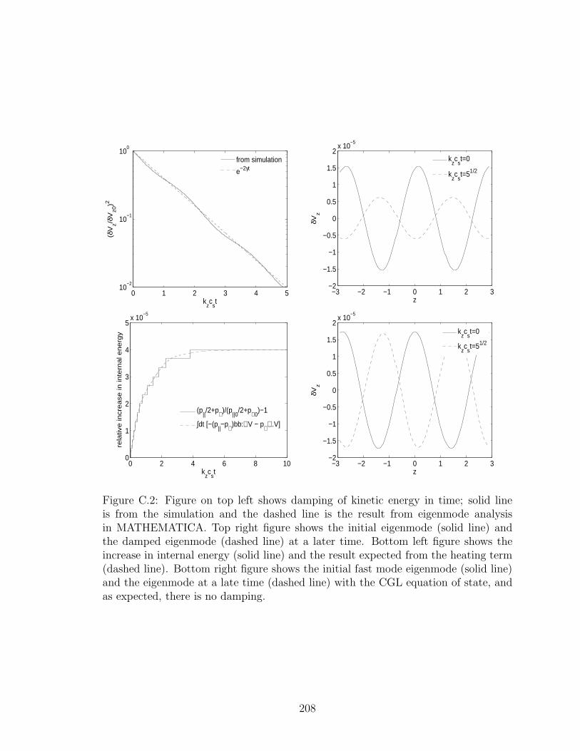
0 1 2 3 4 510

−2

10−1

100

kzc

st

(δV

z/δV

z0)2

from simulation

e−2γt

−3 −2 −1 0 1 2 3−2

−1.5

−1

−0.5

0

0.5

1

1.5

2x 10

−5

z

δVz

kzc

st=0

kzc

st=51/2

0 2 4 6 8 100

1

2

3

4

5x 10

−5

kzc

st

rela

tive

incr

ea

se in

inte

rna

l en

erg

y

(p||/2+p⊥ )/(p

||0/2+p⊥ 0

)−1

∫dt [−(p||−p⊥ )bb:∇ V − p⊥ ∇ .V]

−3 −2 −1 0 1 2 3−2

−1.5

−1

−0.5

0

0.5

1

1.5

2x 10

−5

z

δVz

kzc

st=0

kzc

st=51/2

Figure C.2: Figure on top left shows damping of kinetic energy in time; solid lineis from the simulation and the dashed line is the result from eigenmode analysisin MATHEMATICA. Top right figure shows the initial eigenmode (solid line) andthe damped eigenmode (dashed line) at a later time. Bottom left figure shows theincrease in internal energy (solid line) and the result expected from the heating term(dashed line). Bottom right figure shows the initial fast mode eigenmode (solid line)and the eigenmode at a late time (dashed line) with the CGL equation of state, andas expected, there is no damping.

208

energy. Figure also shows that a fast mode eigenmode in the CGL limit shows no

damping.

Since the magnetic perturbation vanishes for this case, there is no −µ∇‖B Barnes

damping. This leaves only the parallel eE‖ Landau damping. With eE‖ = ikδp‖(me/mi)/n,

assuming cold electrons, Landau damping is hidden in pressure terms in the equation

of motion and the internal energy equation.

C.3.3 Mirror instability in 1-D

The mirror instability criterion in the CGL limit is p⊥/6p‖−1−1/β⊥ > 0 as compared

to the criterion in the kinetic regime, p⊥/p‖−1−1/β⊥ > 0 [110, 180]. We test Landau

closure by initializing an anisotropic pressure (p⊥/p‖ = 2.5, β‖ = 1) which is unstable

according to the kinetic criterion but stable by the CGL criterion. Landau closure

with parameter kL = 12π/L (gives correct kinetic behavior for 6 wavelengths in the

box, for larger wavenumber growth rate is faster than the kinetic result, see Figure

2.1). Figure C.3 shows the results of nonlinear simulations initialized with a small

amplitude random white noise. Pressure anisotropy is reduced to marginality with

time. Particles are trapped in low magnetic field regions due to the mirror force,

and density and magnetic field strengths are anticorrelated. Growth rate increases

linearly with the resolution, as γ ∝ k‖.

For small pressure anisotropy, adiabatic invariance is obeyed and plasma rear-

ranges itself in the form form of mirrors and becomes marginally stable. These 1-D

results are consistent with previous fluid [20] and kinetic [127] studies. Similar 1-D

tests for the firehose instability results have shown results consistent with the previ-

ous kinetic simulations [162]. Here too, the growth rate is proportional to the grid

resolution (as γ ∝ k‖). Fastest growing firehose mode is the one with a parallel

wavenumber. The transverse magnetic field disturbances grow until the plasma be-

comes marginally stable to the firehose instability. A 2-D test for firehose instability

209

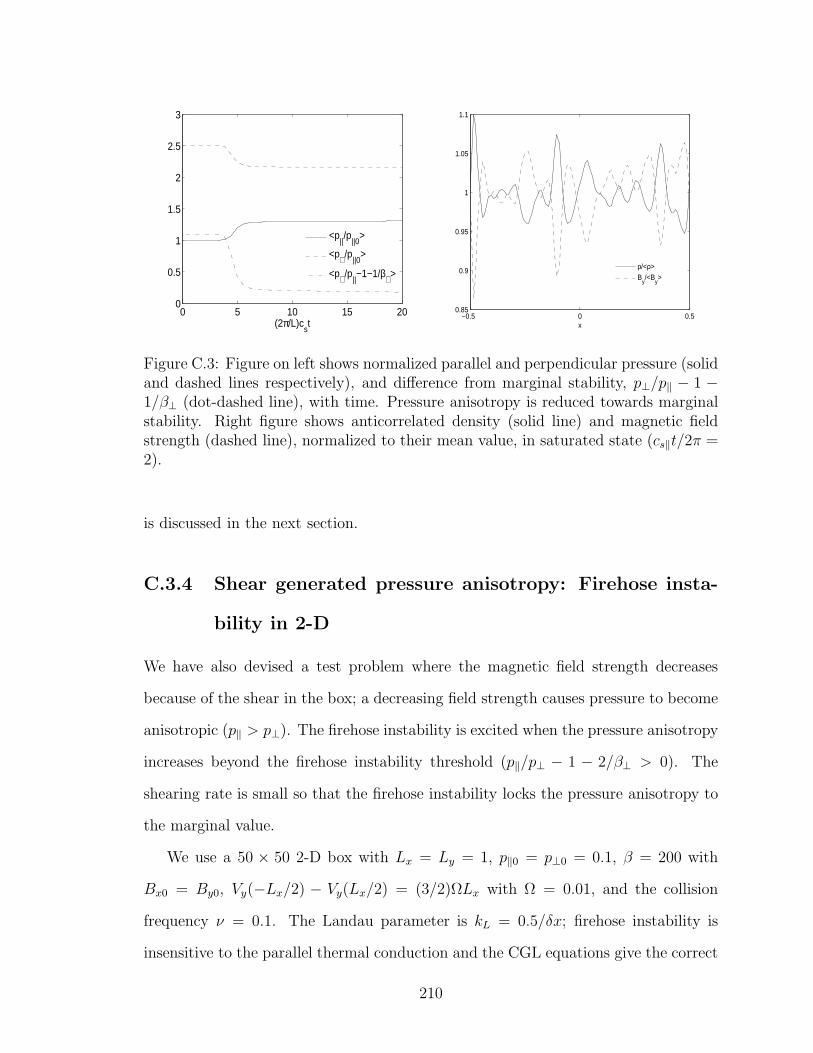
0 5 10 15 200

0.5

1

1.5

2

2.5

3

(2π/L)cst

<p||/p

||0>

<p⊥ /p||0

>

<p⊥ /p||−1−1/β⊥ >

−0.5 0 0.50.85

0.9

0.95

1

1.05

1.1

x

ρ/<ρ>B

y/<B

y>

Figure C.3: Figure on left shows normalized parallel and perpendicular pressure (solidand dashed lines respectively), and difference from marginal stability, p⊥/p‖ − 1 −1/β⊥ (dot-dashed line), with time. Pressure anisotropy is reduced towards marginalstability. Right figure shows anticorrelated density (solid line) and magnetic fieldstrength (dashed line), normalized to their mean value, in saturated state (cs‖t/2π =2).

is discussed in the next section.

C.3.4 Shear generated pressure anisotropy: Firehose insta-

bility in 2-D

We have also devised a test problem where the magnetic field strength decreases

because of the shear in the box; a decreasing field strength causes pressure to become

anisotropic (p‖ > p⊥). The firehose instability is excited when the pressure anisotropy

increases beyond the firehose instability threshold (p‖/p⊥ − 1 − 2/β⊥ > 0). The

shearing rate is small so that the firehose instability locks the pressure anisotropy to

the marginal value.

We use a 50 × 50 2-D box with Lx = Ly = 1, p‖0 = p⊥0 = 0.1, β = 200 with

Bx0 = By0, Vy(−Lx/2) − Vy(Lx/2) = (3/2)ΩLx with Ω = 0.01, and the collision

frequency ν = 0.1. The Landau parameter is kL = 0.5/δx; firehose instability is

insensitive to the parallel thermal conduction and the CGL equations give the correct

210

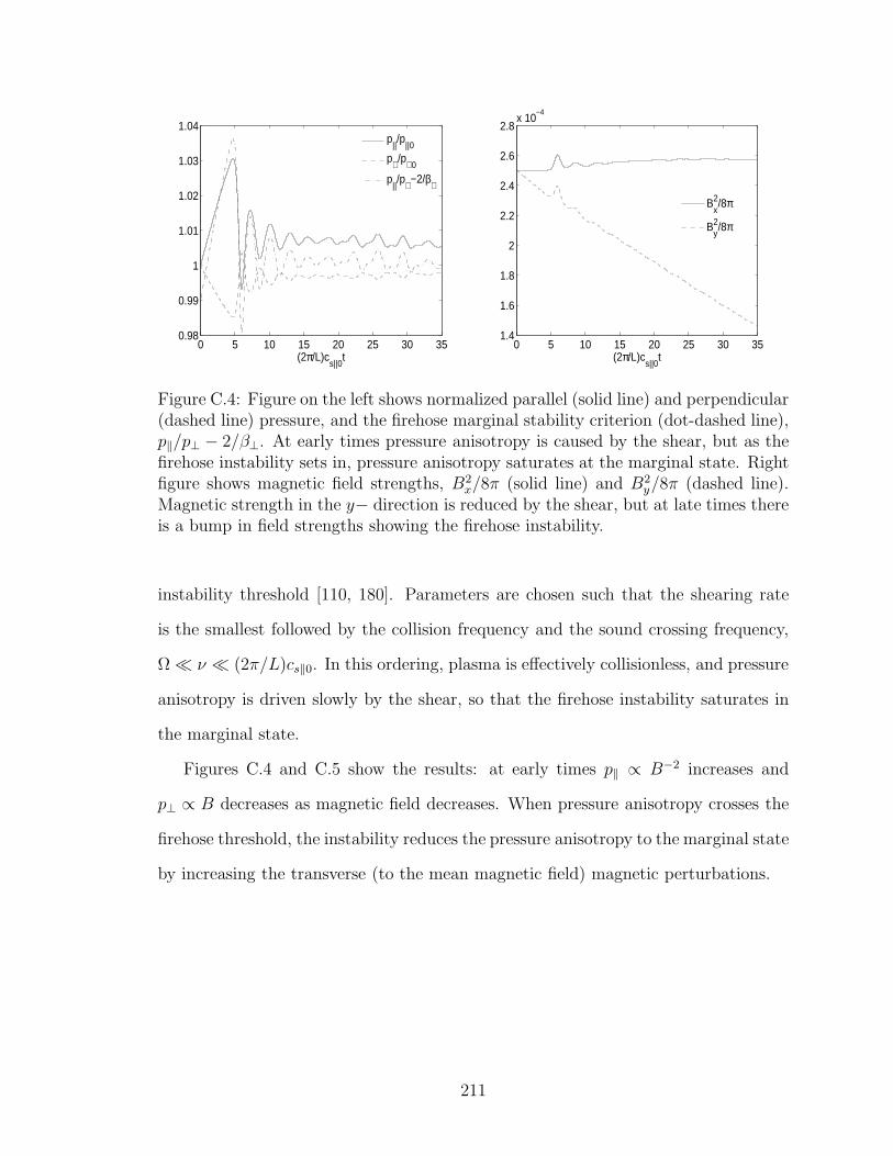
0 5 10 15 20 25 30 350.98

0.99

1

1.01

1.02

1.03

1.04

(2π/L)cs||0

t

p||/p

||0

p⊥ /p⊥ 0

p||/p⊥ −2/β⊥

0 5 10 15 20 25 30 351.4

1.6

1.8

2

2.2

2.4

2.6

2.8x 10

−4

(2π/L)cs||0

t

Bx2/8π

By2/8π

Figure C.4: Figure on the left shows normalized parallel (solid line) and perpendicular(dashed line) pressure, and the firehose marginal stability criterion (dot-dashed line),p‖/p⊥ − 2/β⊥. At early times pressure anisotropy is caused by the shear, but as thefirehose instability sets in, pressure anisotropy saturates at the marginal state. Rightfigure shows magnetic field strengths, B2

x/8π (solid line) and B2y/8π (dashed line).

Magnetic strength in the y− direction is reduced by the shear, but at late times thereis a bump in field strengths showing the firehose instability.

instability threshold [110, 180]. Parameters are chosen such that the shearing rate

is the smallest followed by the collision frequency and the sound crossing frequency,

Ω ≪ ν ≪ (2π/L)cs‖0. In this ordering, plasma is effectively collisionless, and pressure

anisotropy is driven slowly by the shear, so that the firehose instability saturates in

the marginal state.

Figures C.4 and C.5 show the results: at early times p‖ ∝ B−2 increases and

p⊥ ∝ B decreases as magnetic field decreases. When pressure anisotropy crosses the

firehose threshold, the instability reduces the pressure anisotropy to the marginal state

by increasing the transverse (to the mean magnetic field) magnetic perturbations.

211

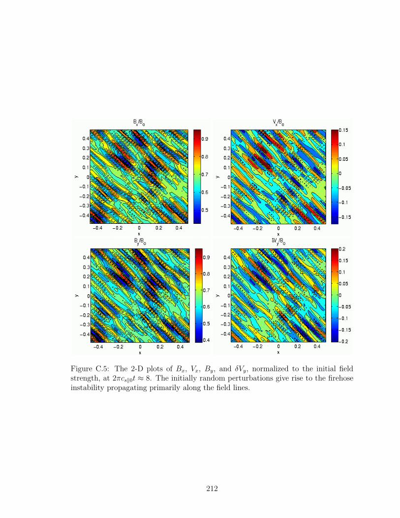
Figure C.5: The 2-D plots of Bx, Vx, By, and δVy, normalized to the initial fieldstrength, at 2πcs‖0t ≈ 8. The initially random perturbations give rise to the firehoseinstability propagating primarily along the field lines.

212

Appendix D

Error analysis

The standard errors in the time averages reported in Table 4.2 and in Figure 4.7 are

estimated by taking into account the finite correlation time for the physical quantities

in the simulation, using techniques recommended by [144]. Given a finite time series,

we want to calculate the ensemble average and the uncertainty around the ensem-

ble average. The standard deviation of the time series does not represent the error

(uncertainty) because the data in the time series are correlated.

For a time series with non-zero correlation time, the standard error for the time

average 〈x〉 =∫

dt x(t)/T of a signal x(t) is given by σ〈x〉 =√

Var(x)/Neff , where

Var(x) =∫

dt (x(t) − 〈x〉)2/T is the variance of x, Neff = T/(2τint) is the effec-

tive number of independent measurements, T = 15 orbits is the averaging time for

the simulations described in Chapter 4, and τint is an estimate of the integrated

autocorrelation time. There are significant subtleties in determining the integrated

autocorrelation time from data. To deal with this, we use a windowing technique as

recommended by [144], using τint =∫ T

0dτ C(τ)W (τ/τw), where C(τ) is the 2-time

correlation function from the data, W (τ/τw) is a smooth window function that cuts

off the integral at τ ∼ τw, and τw ∼√Tτint (this gives results insensitive to the choice

of window width for τint ≪ T ). If windowing is not used, i.e., W = 1, then the

213

integral for τint vanishes; therefore, an appropriate windowing function is necessary.

The two-time autocorrelation function is defined as

C(τ) =1

T

∫ T−τ

0

dtx(t)x(t+ τ), (D.1)

where x = x − 〈x〉. An example of the windowing function is the Hanning window

given by [144]

H(ξ) =1

2[1 + cos(πξ)] , |ξ| < 1 (D.2)

= 0, |ξ| ≥ 1 (D.3)

Winters et. al. [200] found from comparing 3 realizations of shearing box MRI

simulations that the magnetic stress had a variation of approximately ±6.5% after

averaging over 85 orbits. The simulations we show here were averaged over 15 orbits,

so extrapolating from [200] one might expect the uncertainties to be larger by a

factor of ≈√

85/15 ≈ 2.4. This is consistent with the typical error bars we report in

Table 4.2 and Figure 4.7.

214

Appendix E

Entropy condition for an ideal gas

The entropy for an ideal gas is given by S = nV k ln(T 1/(γ−1)/n) + const., where n

is the number density, V the volume, T the temperature, and γ the ratio of specific

heats (= 5/3 for a 3-D mono-atomic gas). The change in entropy that results from

adding an amount of heat dQ to a uniform gas is

dS =nV k

γ − 1

dT

T=dQ

T.

We measure temperature in energy units, so k = 1 from now on. The rate of change

of entropy of a system where number density and temperature can vary in space

(density is assumed to be constant in time) is given by

S ≡ ∂S

∂t= −

∫

dV∇ · qT

= −∫

dVq · ∇TT 2

=

∫

dV nχ|∇‖T |2T 2

≥ 0, (E.1)

where we use an anisotropic heat flux, q = −nχbb∇T , and the integral is evaluated

over the whole space with the boundary contributions assumed to vanish. The local

entropy function is defined as s = −q · ∇T/T 2 can be integrated to calculate the rate

of change of total entropy of the system.

In Chapter 5 we use a related function (the entropy-like function s∗) defined as

215

s∗ ≡ −q · ∇T to limit the symmetric methods using face-pairs, and to prove some

properties of different anisotropic diffusion schemes. The condition −q · ∇T ≥ 0

means that heat always flows from higher to lower temperatures.

216

Bibliography

[1] M. A. Abramowicz, X. Chen, S. Kato, J. P. Lasota, and O. Regev. Thermal

equilibria of accretion disks. Astrophys. J., 438(1):L37, 1995.

[2] N. Afshordi, B. Mukhopadhyay, and R. Narayan. Bypass to Turbulence in

Hydrodynamic Accretion: Lagrangian Analysis of Energy Growth. Astrophys.

J., 629:373, 2005.

[3] E. Agol. Sagittarius A∗ Polarization: No Advection-dominated Accretion Flow,

Low Accretion Rate, and Nonthermal Synchrotron Emission. Astrophys. J.,

538:121, 2000.

[4] D. K. Aitken, J. Greaves, A. Chrysostomou, T. Jenness, W. Holland, J. H.

Hough, D. Pierce-Price, and J. Richer. Detection of Polarized Millimeter and

Submillimeter Emission from Sagittarius A∗. Astrophys. J., 534:173, 2000.

[5] P. J. Armitage. Turbulence and Angular Momentum Transport in Global Ac-

cretion Disk Simulation. Astrophys. J., 501:L189, 1998.

[6] J. Arons. Photon bubbles — Overstability in a magnetized atmosphere. Astro-

phys. J., 388:561, 1992.

[7] F. K. Baganoff, M. W. Bautz, W. N. Brandt, G. Chartas, E. D. Feigelson, G. P.

Garmire, Y. Maeda, M. Morris, G. R. Ricker, L. K. Townsley, and F. Walter.

217

Rapid X-ray flaring from the direction of the supermassive black hole at the

Galactic Centre. Nature, 413(6851):45, 2001.

[8] F. K. Baganoff, Y. Maeda, M. Morris, M. W. Bautz, W. N. Brandt, W. Cui,

J. P. Doty, F. D. Feigelson, G. P. Garmire, S. H. Pravdo, G. R. Ricker, and

L. K. Townsley. Chandra X-ray Spectroscopic Imaging of Sagittarius A∗ and

the Central Parsec of the Galaxy. Astrophys. J., 591(2):891, 2003.

[9] J. Balbas and E. Tadmor. Non-oscillatory central schemes for one- and two-

dimensional MHD equations. II: High-order semi-discrete schemes. SIAM Jour-

nal of Scientific Computation, submitted, 2006.

[10] S. A. Balbus. Stability, Instability, and “Backward” Transport in Stratified

Fluids. Astrophys. J., 534:420, 2000.

[11] S. A. Balbus. Convective and Rotational Stability of a Dilute Plasma. Astro-

phys. J., 562:909, 2001.

[12] S. A. Balbus. Viscous Shear Instability in Weakly Magnetized, Dilute Plasmas.

Astrophys. J., 616:857, 2004.

[13] S. A. Balbus, C. F. Gammie, and J. F. Hawley. Fluctuations, dissipation and

turbulence in accretion discs. Mon. Not. R. Astron. Soc., 271:197, 1994.

[14] S. A. Balbus and J. F. Hawley. A powerful local shear instability in weakly

magnetized disks. I — Linear analysis. Astrophys. J., 376:214, 1991.

[15] S. A. Balbus and J. F. Hawley. A Powerful Local Shear Instability in Weakly

Magnetized Disks. IV. Nonaxisymmetric Perturbations. Astrophys. J., 400:610,

1992.

[16] S. A. Balbus and J. F. Hawley. Instability, turbulence, and enhanced transport

in accretion disks. Rev. Mod. Phys., 70:1, 1998.

218

[17] S. A. Balbus, J. F. Hawley, and J. M. Stone. Nonlinear Stability, Hydrodynam-

ical Turbulence, and Transport in Disks. Astrophys. J., 467:76, 1996.

[18] A. Barnes. Collisionless damping of hydromagnetic waves. Phys. Fluids,

9(8):1483, 1966.

[19] P. J. Basser and D. K. Jones. Diffusion-tensor MRI: theory, experimental design,

and data analysis – a technical review. NMR Biomed., 15:456, 2002.

[20] K. Baumgartel. Fluid approach to mirror mode structures. Planetary Space

Sc., 49:1239, 2001.

[21] B. J. Bayley, S. A. Orszag, and T. Herbert. Instability mechanisms in shear-flow

transition. Ann. Rev. Fluid Mech., 20:359, 1988.

[22] M. A. Beer, S. C. Cowley, and G. W. Hammett. Field-aligned Coordinates for

Nonlinear Simulations of Tokamak Turbulence. Phys. Plasmas, 2:2687, 1995.

[23] M. C. Begelman. Photon Bubbles and the Vertical Structure of Accretion Disks.

Astrophys. J., 643:1065, 2006.

[24] M. C. Begelman and T. Chiueh. Thermal coupling of ions and electrons by

collective effects in two-temperature accretion flows. Astrophys. J., 332:872,

1988.

[25] P. L. Bhatnagar, E. P. Gross, and M. Krook. A model fo collision processes

in gases, 1, small amplitude processes in charged and neutral one-component

systems. Phys. Rev., 94(3):511, 1954.

[26] J. Birn and M. Hesse. Geospace environment modeling (GEM) magnetic re-

connection challenge: Resistive tearing, anisotropic pressure and hall effects. J.

Geophys. Res., 106(A3):3737, 2001.

219

[27] J. A. Biskamp. Magnetohydrodynamic Turbulence. Cambridge Univ. Press,

Cambridge, 2003.

[28] E. G. Blackman, R. F. Penna, and P. Varniere. Empirical relation between an-

gular momentum transport and thermal-to-magnetic pressure ratio in shearing

box simulations. astro-ph/0607119, submitted to Mon. Not. R. Astron. Soc.,

2006.

[29] O. M. Blaes and S. A. Balbus. Local shear instabilities in weakly ionized, weakly

magnetized disks. Astrophys. J., 421(1):163, 1994.

[30] O. M. Blaes and A. Socrates. Local Dynamical Instabilities in Magnetized,

Radiation Pressure-supported Accretion Disks. Astrophys. J., 553(2):287, 2001.

[31] R. D. Blandford and M. C. Begelman. On the fate of gas accreting at a low

rate on to a black hole. Mon. Not. R. Astron. Soc., 303(1):L1, 1999.

[32] R. D. Blandford and M. C. Begelman. Two-dimensional adiabatic flows on to

a black hole — I. fluid accretion. Mon. Not. R. Astron. Soc., 349(1):68, 2003.

[33] R. D. Blandford and D. G. Payne. Hydromagnetic flows from accretion discs

and the production of radio jets. Mon. Not. R. Astron. Soc., 199:883, 1982.

[34] R. D. Blandford and R. L. Znajek. Electromagnetic extraction of energy from

Kerr black holes. Mon. Not. R. Astron. Soc., 179:433, 1977.

[35] H. Bondi. On spherically symmetrical accretion. Mon. Not. R. Astron. Soc.,

112:195, 1952.

[36] G. C. Bower, M. C. H. Wright, H. Falcke, and D. C. Backer. Interferometric

Detection of Linear Polarization from Sagittarius A∗ at 230 GHz. Astrophys.

J., 588:331, 2003.

220

[37] S. I. Braginskii. Reviews of Plasma Physics, volume 1, page 205. Consultants

Bureau, 1965.

[38] A. Brandenburg, A. Nordlund, R. F. Stein, and U. Torkelsson. Dynamo-

generated Turbulence and Large-Scale Magnetic Fields in a Keplerian Shear

Flow. Astrophys. J., 446:741, 1995.

[39] M. Burin and H. Ji. manuscript in preparation. private communication, 2006.

[40] J. Candy and R. E. Waltz. Anomalous Transport in the DIII-D Tokamak

Matched by Supercomputer Simulation. Phys. Rev. Lett., 91:045001, 2003.

[41] V. Caselles, J.M. Morel, G. Sapiro, and A. Tannenbaum. Introduction to the

special issue on partial differential equations and geometry-driven diffusion in

image processing and analysis. IEEE Trans. on Image Processing, 7:269, 1998.

[42] G. D. Chagelishvili, J. P. Zahn, A. G. Tevzadze, and J. G. Lominadze. On

hydrodynamic shear turbulence in Keplerian disks: Via transient growth to

bypass transition. Astron. Astrophys., 402:401, 2003.

[43] B. Chandran and S. C. Cowley. Thermal Conduction in a Tangled Magnetic

Field. Phys. Rev. Lett., 80(14):3077, 1998.

[44] S. Chandrasekhar. The stability of non-dissipative Couette flow in hydromag-

netics. Proc. Nat. Acad. Sci., 46:253, 1960.

[45] S. Chandrasekhar. Hydrodynamic and Hydromagnetic Stability. Oxford Univ.

Press, London, 1961.

[46] Z. Chang and J. D. Callen. Unified fluid/kinetic description of plasma microin-

stabilities. part I: Basic equations in a sheared slab geometry. Phys. Fluids B,

4(5):1167, 1992.

221

[47] S. Chapman and T. G. Cowling. The Mathematical Theory of Non-Uniform

Gases. Cambridge Univ. Press, Cambridge, 1970.

[48] C. F. Chew, M. L. Goldberger, and F. E. Low. The Boltzmann equation and the

one-fluid hydromagnetic equations in the absence of particle collisions. Proc.

R. Soc. London A, 236:112, 1956.

[49] S. C. Cowley, R. M. Kulsrud, and R. Sudan. Considerations of ion-temperature-

gradient-driven turbulence. Phys. Fluids B, 3:2767, 1991.

[50] J. A. Crawford and R. P. Craft. An Intrepretation of AE Aquarii. Astrophys.

J., 123:44, 1956.

[51] A. M. Dimits. private communication, 1994. A.M. Dimits was the first to

suggest using Pade approximations for the Landau damping operator, in private

communications to G.W. Hammett in the mid 1990’s.

[52] A. M. Dimits, G. Bateman, M. A. Beer, B. I. Cohen, W. Dorland, G. W. Ham-

mett, C. Kim, J. E. Kinsey, M. Kotschenreuther, A. H. Kritz, L. L. Lao, J. Man-

drekas, W. M. Nevins, S. E. Parker, A. J. Redd, D. E. Shumaker, R. Sydora,

and J. Weiland. Comparisons and physics basis of tokamak transport models

and turbulence simulations. Phys. Plasmas, 7(3):969, 2000.

[53] W. Dorland, F. Jenko, M. Kotschenreuther, and B.N. Rogers. Electron tem-

perature gradient turbulence. Phys. Rev. Lett., 85:5579, 2000.

[54] W. D. Dorland. Gyrofluid Models of Plasma Turbulence. PhD thesis, Princeton

Univ., 1993.

[55] A. A. Esin, J. E. McClintock, and R. Narayan. Advection-dominated Accretion

and the Spectral States of Back Hole X-Ray Binaries: Application to Nova

MUSCAE 1991. Astrophys. J., 489:865, 1997.

222

[56] A. C. Fabian, K. Iwasawa, C. S. Reynolds, and A. J. Young. Broad Iron Lines

in Active Galactic Nuclei. Pub. Astron. Soc. Pacific, 112(775):1145, 2000.

[57] A. C. Fabian and M. J. Rees. The accretion luminosity of a massive black hole

in an elliptical galaxy. Mon. Not. R. Astron. Soc., 277(2):L55, 1995.

[58] L. Ferrarese and D. Merritt. A Fundamental Relation between Supermassive

Black Holes and Their Host Galaxies. Astrophys. J., 539(1):L9, 2000.

[59] T. P. Fleming, J. M. Stone, and J. F. Hawley. The Effect of Resistivity on

the Nonlinear Stage of the Magnetorotational Instability in Accretion Disks.

Astrophys. J., 530:464, 2000.

[60] E. A. Foote and R. M. Kulsrud. Electromagnetic waves in high β plasmas.

Astrophys. J., 233:302, 1979.

[61] J. Frank, A. King, and D. Raine. Accretion Power in Astrophysics. Cambridge

Univ. Press, Cambridge, 2002.

[62] U. Frisch. Turbulence: The legacy of A. N. Kolmogorov. Cambridge Univ.

Press, Cambridge, 1995.

[63] C. F. Gammie. Layered Accretion in T Tauri Disks. Astrophys. J., 457:355,

1996.

[64] C. F. Gammie. Photon bubbles in accretion discs. Astrophys. J., 297:929, 1998.

[65] T. A. Gardiner and J. M. Stone. An unsplit Godunov method for ideal MHD

via constrained transport. J. Comp. Phys., 205(2):509, 2005.

[66] S. P. Gary, B. J. Anderson, R. E. Denton, S. A. Fuselier, M. E. McKean,

and D. Winske. Ion anisotropies in the magnetosheath. Geophys. Res. Lett.,

20(17):1767, 1993.

223

[67] S. P. Gary and M. A. Lee. The ion cyclotron anisotropy instability and the

inverse correlation between proton anisotropy and proton beta. J. Geophys.

Res., 99(A6):11297, 1994.

[68] S. P. Gary and J. Wang. Whistler instability: electron anisotropy upper bound.

J. Geophys. Res., 101(A5):10749, 1996.

[69] S. P. Gary, J. Wang, D. Winske, and S. A. Fuselier. Proton temperature

anisotropy upper bound. J. Geophys. Res., 102(A12):27159, 1997.

[70] K. Gebhardt and et al. A Relationship between Nuclear Back Hole Mass and

Galaxy Velocity Dispersion. Astrophys. J., 539(1):L13, 2000.

[71] A. M. Ghez, G. Duchene, K. Matthews, S. D. Hornstein, A. Tanner, J. Larkin,

M. Morris, E. E. Becklin, S. Salim, T. Kremenek, D. Thompson, B. T. Soifer,

G. Neugebauer, and I. McLean. The First Measurement of Spectral Lines in

a Short-Period Star Bound to the Galaxy’s Central Black Hole: A Paradox of

Youth. Astrophys. J., 586(2):L127, 2003.

[72] P. Goldreich, J. Goodman, and R. Narayan. The stability of accretion tori. I

— Long-wavelength modes of slender tori. Mon. Not. R. Astron. Soc., 221:339,

1986.

[73] P. Goldreich and S. Sridhar. Toward a theory of interstellar turbulence. 2:

Strong Alfvenic turbulence. Astrophys. J., 438(2):763, 1995.

[74] H. Goldstein, C. P. Poole, and J. L. Safko. Classical Mechanics. Addison

Wesley, 2002.

[75] J. Goodman and G. Xu. Parasitic instabilities in magnetized, differentially

rotating disks. Astrophys. J., 432(1):213, 1994.

224

[76] S. Gunter, Q. Yu, J. Krger, and K. Lackner. Modelling of heat transport in

magnetised plasmas using non-aligned coordinates. J. Comp. Phys., 209(1):354,

2005.

[77] G. W. Hammett, M. A. Beer, W. Dorland, S. C. Cowley, and S. A. Smith.

Developments in the gyrofluid approach to tokamak turbulence simulations.

Plasma Phys. Controlled Fusion, 35(8):973, 1993.

[78] G. W. Hammett, W. Dorland, and F. W. Perkins. Fluid models of phase

mixing, Landau damping, and nonlinear gyrokinetic dynamics. Phys. Fluids B,

4(7):2052, 1992.

[79] G. W. Hammett and F. W. Perkins. Fluid Moment Models for Landau Damping

with Application to the Ion-Temperature-Gradient Instability. Phys. Rev. Lett.,

64(25):3019, 1990.

[80] A. Hasegawa. Drift mirror instability in the magnetosphere. Phys. Fluids,

12(12):2642, 1969.

[81] J. F. Hawley. Global Magnetohydrodynamical Smulations of Accretion Tori.

Astrophys. J., 528:462, 2000.

[82] J. F. Hawley and S. A. Balbus. A Powerful Local Shear Instability in Weakly

Magnetized Disks. II. Nonlinear Evolution. Astrophys. J., 376:223, 1991.

[83] J. F. Hawley and S. A. Balbus. The Dynamical Structure of Nonradiative Black

Hole Accretion Flows. Astrophys. J., 573(2):738, 2002.

[84] J. F. Hawley, S. A. Balbus, and J. M. Stone. A Magnetohydrodynamic Nonra-

diative Accretion Flow in Three Dimensions. Astrophys. J., 554(1):L49, 2001.

[85] J. F. Hawley, S. A. Balbus, and W. F. Winters. Local Hydrodynamic Stability

of Accretion Disks. Astrophys. J., 518:394, 1999.

225

[86] J. F. Hawley, C. F. Gammie, and S. A. Balbus. Local Three-dimensional Magne-

tohydrodynamic Simulations of Accretion Disks. Astrophys. J., 440:372, 1995.

[87] J. F. Hawley, C. F. Gammie, and S. A. Balbus. Local Three-dimensional Sim-

ulations of an Accretion Disk Hydromagnetic Dynamo. Astrophys. J., 464:690,

1995.

[88] J. F. Hawley and J. M. Stone. Nonlinear Evolution of the Magnetorotational

Instability in Ion-Neutral Disks. Astrophys. J., 501:758, 1998.

[89] L. C. Ho. The Sectral Energy Distributions of Low-Luminosity Active Galactic

Nuclei. Astrophys. J., 516(2):672, 1999.

[90] L. C. Ho, E. D. Feigelson, L. K. Townsley, R. M. Sambruna, G. P. Garmire,

W. N. Brandt, A. V. Filippenko, R. E. Griffiths, A. F. Ptak, and W. L. W.

Sargent. Detection of Nuclear X-ray Sources in Nearby Galaxies with Chandra.

Astrophys. J., 549(1):L51, 2001.

[91] J. D. Huba. NRL Plasma Formulary. The Office of Naval Research, 2000.

[92] S. Ichimaru. Bimodal behavior of accretion disks — theory and application to

Cygnus X-1 transitions. Astrophys. J., 214:840, 1977.

[93] J. Igea and A. E. Glassgold. X-Ray Ionization of the Disks of Young Stellar

Objects. Astrophys. J., 518:848, 1999.

[94] I. V. Igumenshchev and M. A. Abramowicz. Rotating accretion flows around

black holes: convection and variability. Mon. Not. R. Astron. Soc., 303(2):309,

1999.

[95] I. V. Igumenshchev, R. Narayan, and M. A. Abramowicz. Three-dimensional

Magnetohydrodynamic Simulations of Radiatively Iefficient Accretion Flows.

Astrophys. J., 592(2):1042, 2003.

226

[96] T. Islam and S. A. Balbus. Dynamics of the Mgnetoviscous Istability. Astrophys.

J., 633:328, 2005.

[97] F. Jenko, W. Dorland, M. Kotschenreuther, and B.N. Rogers. Electron tem-

perature gradient driven turbulence. Phys. Plasmas, 7:1904, 2000.

[98] J. C. Kasper, A. J. Lazarus, and S. P. Gary. Wind/SWE observations of firehose

constraint on solar wind proton temperature anisotropy. Geophys. Res. Lett.,

29(17):20–1, 2002.

[99] C. F. Kennel and H. E. Petchek. Limit on stably trapped particle fluxes. J.

Geophys. Res., 71:1, 1966.

[100] C. F. Kennel and R. Z. Sagdeev. Collisionless shock waves in high β plasmas,

1. J. Geophys. Res., 72(13):3303, 1967.

[101] M. G. Kivelson and D. J. Southwood. Mirror instability II: The mechanism of

nonlinear saturation. J. Geophys. Res., 101(A8):17365, 1996.

[102] S. S. Komissarov. Observations of the Blandford-Znajek process and the mag-

netohydrodynamic Penrose process in computer simulations of black hole mag-

netospheres. Mon. Not. R. Astron. Soc., 359(3):801, 2005.

[103] A. Koratkar and O. Blaes. The Ultraviolet and Optical Continuum Emission

in Active Galactic Nuclei: The Status of Accretion Disks. Pub. Astron. Soc.

Pacific, 111(755):1, 1999.

[104] N. A. Krall and A. W. Trivelpiece. Principles of Plasma Physics. San Francisco

Press, San Francisco, 1986.

[105] J. H. Krolik and J. F. Hawley. Magnetically Driven Jets in the Kerr Metric.

Astrophys. J., 641:103, 2006.

227

[106] J. H. Krolik and E. G. Zweibel. The weak-field limit of the magnetorotational

instability. Astrophys. J., 644:651, 2006.

[107] M. D. Kruskal and C. R. Oberman. On the stability of plasma in static equi-

librium. Phys. Fluids, 1(4):275, 1958.

[108] G. P. Kuiper. On the Interpretation of β Lyrae and Other Close Binaries.

Astrophys. J., 93:133, 1941.

[109] R. M. Kulsrud. General stability theory in plasma physics. In M. N. Rosenbluth,

editor, Proceedings of the international school of Physics, Enrico Fermi, Course

XXV, Advanced Plasma Theory. North Holland, 1962.

[110] R. M. Kulsrud. Handbook of Plasma Physics, volume 1, page 115. North

Holland, 1983.

[111] R. M. Kulsrud. Plasma Physics for Astrophysics. Princeton Univ. Press, Prince-

ton, 2005.

[112] A. Kurganov and E. Tadmor. New high-resolution central schemes for nonlinear

conservation laws and convection-diffusion equations. Astrophys. J., 93:133,

1941.

[113] L. D. Landau. On the vibrations of the electronic plasma. J. Phys. USSR,

10:26, 1946.

[114] J. P. Lasota, M. A. Abramowicz, X. Chen, J. Krolik, R. Narayan, and I. Yi.

Is the Accretion Flow in NGC 4258 Advection Dominated? Astrophys. J.,

462:142, 1996.

[115] G. Lesur and P. Y. Longaretti. On the relevance of subcritical hydrodynamic

turbulence to accretion disk transport. Astron. Astrophys., 444(1):25, 2005.

228

[116] R. J. Leveque. Finite Volume Methods for Hyperbolic Problems. Cambridge

Univ. Press, Cambridge, 2002.

[117] C. D. Levermore and G. C. Pomraning. A flux-limited diffusion theory. Astro-

phys. J., 248(1):321, 1981.

[118] D. N. C. Lin and J. Papaloizou. On the structure and evolution of the primordial

solar nebula. Mon. Not. R. Astron. Soc., 191:37, 1980.

[119] M. Loewenstein, R. F. Mushotzky, L. Angelini, K. A. Arnaud, and E. Quataert.

Chandra Limits on X-Ray Emission Associated with the Supermassive Black

Holes in Three Giant Elliptical Galaxies. Astrophys. J., 555:21L, 2001.

[120] D. Lynden-Bell. Galactic Nuclei as Collapsed Old Quasars. Nature, 223:690,

August 1969.

[121] D. Lynden-Bell and J. E. Pringle. The evolution of viscous discs and the origin

of the nebular variables. Mon. Not. R. Astron. Soc., 168:603, 1974.

[122] J. Magorrian, S. Tremaine, D. Richstone, R. Bender, G. Bower, A. Dressler,

S. M. Faber, K. Gebhardt, R. Green, C. Grillmair, J. Kormendy, and T. Lauer.

The Demography of Massive Dark Objects in Galaxy Centers. Astron. J.,

115(6):2285, 1998.

[123] E. Marsch, R. Schwenn, H. Rosenbauer, K. H. Muehlhaeuser, W. Pilipp, and

F. M. Neubauer. Solar wind protons — Three-dimensional velocity distributions

and derived plasma parameters measured between 0.3 and 1 AU. J. Geophys.

Res., 87:52, 1982.

[124] R. Matsumoto and T. Tajima. Magnetic viscosity by localized shear flow insta-

bility in magnetized accretion disks. Astrophys. J., 445:767, 1995.

229

[125] T. Di Matteo, R. M. Johnstone, S. W. Allen, and A. C. Fabian. Accretion

onto Nearby Supermassive Black Holes: Chandra Constraints on the Dominant

Cluster Galaxy NGC 6166. Astrophys. J., 550(1):L19, 2001.

[126] N. Mattor. Can Landau-fluid models describe nonlinear Landau damping. Phys.

Fluids B, 4(12):3952, 1992.

[127] M. E. McKean, S. P. Gary, and D. Winske. Kinetic physics of the mirror

instability. J. Geophys. Res., 98(A12):21313, 1993.

[128] J. C. McKinney and C. F. Gammie. A Measurement of the Electromagnetic

Luminosity of a Kerr Black Hole. Astrophys. J., 611(2):977, 2004.

[129] F. Melia. An accreting black hole model for Sagittarius A. Astrophys. J.,

387:L25, 1992.

[130] K. Menou. Hot Accretion With Saturated Conduction. astro-ph/0507189, 2005.

[131] D. Mihalas and B. W. Mihalas. Foundations of Radiation Hydrodynamics. Ox-

ford Univ. Press, 1985.

[132] K. A. Miller and J. M. Stone. The Formation and Structure of a Strongly

Magnetized Corona above a Weakly Magnetized Accretion Disk. Astrophys. J.,

534(1):398, 2000.

[133] C. W. Misner, K. S. Thorne, and J. A. Wheeler. Gravitation. Freeman, 1973.

[134] M. Miyoshi, J. Moran, J. Herrnstein, L. Greenhill, N. Nakai, P. Diamond, and

M. Inoue. Evidence for a Black-Hole from High Rotation Velocities in a Sub-

Parsec Region of NGC4258. Nature, 373(6510):127, 1995.

[135] D. C. Montgomery and D. A. Tidman. Plasma Kinetic Theory. Mc-Graw Hill,

1964.

230

[136] P. Mrazek and M. Navara. Consistent positive directional splitting of anisotropic

diffusion. In Proc. of Computer Vision Winter Workshop, page 37, Bled, Slove-

nia, 2001. http://www.mia.uni-saarland.de/mrazek/Publications/Mrazek-

cvww01.pdf.

[137] F. Najarro, A. Krabbe, R. Genzel, D. Lutz, R. P. Kudritzki, and D. J. Hillier.

Quantitative spectroscopy of the HeI cluster in the Galactic center. Astron.

Astrophys., 325:700, 1997.

[138] R. Narayan. Unsolved Problems in Astrophysics, page 301. Princeton Univ.

Press, Princeton, 1997.

[139] R. Narayan. Black holes: Sparks of interest. Nature, 425(6961):908, 2003.

[140] R. Narayan, R. Mahadevan, and E. Quataert. Theory of Black Hole Accretion

Disks, page 148. Cambridge Univ. Press, 1998.

[141] R. Narayan and I. Yi. Advection-dominated accretion: A self-similar solution.

Astrophys. J., 428(1):L13, 1994.

[142] R. Narayan and I. Yi. Advection-dominated accretion: Self-similarity and bipo-

lar outflow. Astrophys. J., 444(1):231, 1995.

[143] H. Nessyahu and E. Tadmor. Non-oscillatory central differencing for hyperbolic

conservation laws. J. Comp. Phys., 87:408, 1990.

[144] W. Nevins. A Statistical Analysis of ITG Turbulence. manuscript in prepara-

tion, 2005.

[145] B. Paczynski and P. J. Wiita. Thick accretion disks and supercritical luminosi-

ties. Astron. Astrophys., 88:23, 1980.

231

[146] J. C. B. Papaloizou and J. E. Pringle. The dynamical stability of differentially

rotating discs with constant specific angular momentum. Mon. Not. R. Astron.

Soc., 208:721, 1984.

[147] S. E. Parker, W. Dorland, R. A. Santoro, M. A. Beer, Q. P. Liu, W. W. Lee,

and G. W. Hammett. Comparisons of gyrofluid and gyrokinetic simulations.

Phys. Plasmas, 1(5):1461, 1994.

[148] I. J. Parrish and J. M. Stone. Nonlinear Evolution of the Magnetothermal

Instability in Two Dimensions. Astrophys. J., 633:334, 2005.

[149] U. Pen, C. D. Matzner, and S. Wong. The Fate of Nonradiative Magnetized Ac-

cretion Flows: Magnetically Frustrated Convection. Astrophys. J., 596(2):L207,

2003.

[150] M. E. Pessah, C. Chan, and D. Psaltis. The signature of the magnetorotational

instability in the Reynolds and Maxwell stress tensors in accretion discs. astro-

ph/0603178, submitted to Mon. Not. R. Astron. Soc., 2006.

[151] R. A. Piontek and E. C. Ostriker. Saturated-State Turbulence and Structure

from Thermal and Magnetorotational Instability in the ISM: Three-dimensional

Numerical Simulations. Astrophys. J., 629:849, 2005.

[152] K. H. Prendergast and G. R. Burbidge. On the Nature of Some Galactic X-Ray

Sources. Astrophys. J., 151:L83, 1968.

[153] J. E. Pringle. Accretion disks in astrophysics. Ann. Rev. Astron. Astrophys.,

19:137, 1981.

[154] D. Proga and M. C. Begelman. Accretion of Low Angular Momentum Material

onto Black Holes: Two-dimensional Hydrodynamical Inviscid Case. Astrophys.

J., 582(1):69, 2003.

232

[155] D. Proga and M. C. Begelman. Accretion of Low Angular Momentum Material

onto Black Holes: Two-dimensional Magnetohydrodynamic Case. Astrophys.

J., 592(2):767, 2003.

[156] E. Quataert. Radiatively Inefficient Accretion Flow Models of Sgr A∗. As-

tronom. Nachr., 324:435, 2003.

[157] E. Quataert. A Dynamical Model for Hot Gas in the Galactic Center. Astrophys.

J., 613(1):322, 2004.

[158] E. Quataert, W. Dorland, and G. W. Hammett. The Magnetorotational Insta-

bility in a Collisionless Plasma. Astrophys. J., 577(1):524, 2002.

[159] E. Quataert and A. Gruzinov. Constraining the Accretion Rate onto Sagittarius

A∗ Using Linear Polarization. Astrophys. J., 545:842, 2000.

[160] E. Quataert and A. Gruzinov. Convection-dominated Accretion Flows. Astro-

phys. J., 539(2):809, 2000.

[161] E. Quataert and R. Narayan. Spectral Models of Advection-dominated Accre-

tion Flows with Winds. Astrophys. J., 520(1):298, 1999.

[162] K. B. Quest and V. D. Shapiro. Evolution of the fire-hose instability: Linear

theory and wave-wave coupling. J. Geophys. Res., 101(A11):24457, 1996.

[163] M. J. Rees, E. S. Phinney, M. C. Begelman, and R. D. Blandford. Ion-supported

tori and the origin of radio jets. Nature, 295:17, 1982.

[164] D. Richard and J. P. Zahn. Turbulence in differentially rotating flows. What can

be learned from the Couette-Taylor experiment. Astron. Astrophys., 347:734,

1999.

[165] M. N. Rosenbluth and N. Rostoker. Theoretical structure of plasma equations.

Phys. Fluids, 2(1):23, 1959.

233

[166] D. Ryu and J. Goodman. Convective instability in differentially rotating disks.

Astrophys. J., 388:438, 1992.

[167] T. Sano, S. Inutsuka, N. J. Turner, and J. M. Stone. Angular Momentum

Transport by Magnetohydrodynamic Turbulence in Accretion Disks: Gas Pres-

sure Dependence of the Saturation Level of the Magnetorotational Instability.

Astrophys. J., 605(1):321, 2004.

[168] T. Sano, S. M. Miyama, T. Umebayashi, and T. Nakano. Magnetorotational

Instability in Protoplanetary Disks. II. Ionization State and Unstable Regions.

Astrophys. J., 543:486, 2000.

[169] T. Sano and J. M. Stone. The Effect of the Hall Term on the Nonlinear Evo-

lution of the Magnetorotational Instability. I. Local Axisymmetric Simulations.

Astrophys. J., 570(1):314, 2002.

[170] A. A. Schekochihin, S. C. Cowley, R. M. Kulsrud, G. W. Hammett, and

P. Sharma. Plasma Instabilities and Magnetic Field Growth in Clusters of

Galaxies. Astrophys. J., 629(1):139, 2005.

[171] R. Schodel, T. Ott, R. Genzel, R. Hofmann, M. Lehnert, A. Eckart,

N. Mouawad, T. Alexander, M. J. Reid, R. Lenzen, M. Hartung, F. Lacombe,

D. Rouan, E. Gendron, G. Rousset, A.-M. Lagrange, W. Brandner, N. Ageorges,

C. Lidman, A. F. M. Moorwood, J. Spyromilio, N. Hubin, and K. M. Menten.

A star in a 15.2-year orbit around the supermassive black hole at the centre of

the milky way. Nature, 419(6908):694, 2002.

[172] B. F. Schutz. A First Course in General Relativity. Cambridge Univ. Press,

Cambridge, 1985.

[173] B. D. Scott. Free-energy conservation in local gyrofluid models. Phys. Plasmas,

12(10):102307, 2005.

234

[174] N. I. Shakura and R. A. Sunyaev. Black holes in binary systems. Observational

appearance. Astron. Astrophys., 24:337, 1973.

[175] P. Sharma and G. W. Hammett. Anisotropic conduction with large temperature

gradients. to be submitted to J. Comp. Phys., 2006.

[176] P. Sharma, G. W. Hammett, and E. Quataert. Transition from Collisionless to

Collisional Magnetorotational Instability. Astrophys. J., 596:1121, 2003.

[177] P. Sharma, G. W. Hammett, E. Quataert, and J. M. Stone. Shearing Box

Simulations of the MRI in a Collisionless Plasma. Astrophys. J., 637:952, 2006.

[178] K. Shibata and Y. Uchida. A magnetodynamic mechanism for the formation of

astrophysical jets. ii - dynamical processes in the accretion of magnetized mass

in rotation. Pub. Astron. Soc. Japan, 38:631, 1986.

[179] S. A. Smith. Dissipative Closures for Statistical Moments, Fluid Moments, &

Subgrid Scales in Plasma Turbulence. PhD thesis, Princeton Univ., 1997.

[180] P. B. Snyder, G. W. Hammett, and W. Dorland. Landau fluid models of colli-

sionless magnetohydrodynamics. Phys. Plasmas, 4(11):3974, 1997.

[181] C. R. Sovinec, A. H. Glasser, T. A. Gianakon, D. C. Barnes, R. A. Nebel, S. E.

Kruger, D. D. Schnack, S. J. Plimpton, A. Tarditi, and M. S. Chu. Nonlinear

magnetohydrodynamics simulation using high-order finite elements. J. Comp.

Phys., 195(1):355, 2004.

[182] T. H. Stix. Waves in Plasmas. AIP Press, New York, 1992.

[183] J. M. Stone and S. A. Balbus. Angular Momentum Transport in Accretion

Disks via Convection. Astrophys. J., 464:364, 1996.

235

[184] J. M. Stone, J. F. Hawley, C. F. Gammie, and S. A. Balbus. Three-dimensional

magnetohydrodynamical simulations of vertically stratified accretion disks. As-

trophys. J., 463:656, 1996.

[185] J. M. Stone and M. L. Norman. ZEUS-2D: A radiation magnetohydrodynamics

code for astrophysical flows in two space dimensions. I. The hydrodynamic

algorithms and tests. Astrophys. J. Suppl., 80(2):753, 1992.

[186] J. M. Stone and M. L. Norman. ZEUS-2D: A radiation magnetohydrodynamics

code for astrophysical flows in two space dimensions. II. The magnetohydrody-

namic algorithms and tests. Astrophys. J. Suppl., 80(2):791, 1992.

[187] J. M. Stone and M. L. Norman. Numerical simulations of magnetic accretion

disks. Astrophys. J., 433:946, 1994.

[188] J. M. Stone and J. E. Pringle. Magnetohydrodynamical non-radiative accretion

flows in two dimensions. Mon. Not. R. Astron. Soc., 528:462, 2001.

[189] J. M. Stone, J. E. Pringle, and M. C. Begelman. Hydrodynamical non-radiative

accretion flows in two dimensions. Mon. Not. R. Astron. Soc., 310:1002, 1999.

[190] T. Tanaka and K. Menou. Hot Accretion Hot Accretion With Conduction:

Spontaneous Thermal Outflows With Saturated Conduction. astro-ph/0604509,

2006.

[191] H. Tennekes and J. L. Lumley. A First Course in Turbulence. The MIT Press,

Cambridge, 1972.

[192] B. T. Tsurutani, E. J. Smith, R. R. Anderson, K. W. Ogilvie, J. D. Scudder,

D. N. Baker, and S. J. Bame. Lion roars and nonoscillatory drift mirror waves

in the magnetosheath. J. Geophys. Res,, 87:6060, 1982.

236

[193] N. J. Turner, O. M. Blaes, A. Socrates, M. C. Begelman, and S. W. Davis. The

Effects of Photon Bubble Instability in Radiation-dominated Accretion Disks.

Astrophys. J., 624:267, 2005.

[194] N. J. Turner, J. M. Stone, J. H. Krolik, and T. Sano. Local Three-dimensional

Simulations of Magnetorotational Instability in Radiation-dominated Accretion

Disks. Astrophys. J., 593:992, 2003.

[195] O. M. Umurhan and O. Regev. Hydrodynamic stability of rotationally sup-

ported flows: Linear and nonlinear 2D shearing box results. Astron. Astrophys.,

427:855, 2004.

[196] B. van Leer. Towards the Ultimate Conservative Difference Scheme V, A Second

Order Sequel to Gudonov’s Method. J. Comp. Phys., 32:101, 1979.

[197] E. P. Velikhov. Stability of an ideally conducting liquid flowing between cylin-

ders rotating in a magnetic field. Soviet Phys.-JETP, 36:1398, 1959.

[198] J. P. De Villiers. Accretion Disks in Large-scale Magnetic Fields. astro-

ph/0605744, 2006.

[199] J. P. De Villiers, J. F. Hawley, and J. H. Krolik. Magnetically Driven Accretion

Flows in the Kerr Metric. I. Models and Overall Structure. Astrophys. J.,

599(2):1238, 2003.

[200] W. F. Winters, S. A. Balbus, and J. F. Hawley. Chaos in turbulence driven by

the magnetorotational instability. Mon. Not. R. Astron. Soc., 340(2):519, 1992.

237