Embed Size (px)
Citation preview

rrlabcsuni-klde
Karsten Berns
Robotics Research Lab
Department of Computer Science
University of Kaiserslautern Germany
Kinematics and Dynamics of Mobile Robots
rrlabcsuni-klde
KaiserslauternGermany
Kaiserslautern
Frankfurt
Berlin
Hamburg
Bremen
Hanover
Cologne
Stuttgart
Munich
Braunschweig
Federal Republic of Germany
bull Deutschland
bull 16 constituent states
bull area of 357386 square
kilometres
bull (137988 sq mi)
bull 83 million inhabitants
bull Capital Berlin
(52deg31primeN 13deg23primeE)
rrlabcsuni-klde
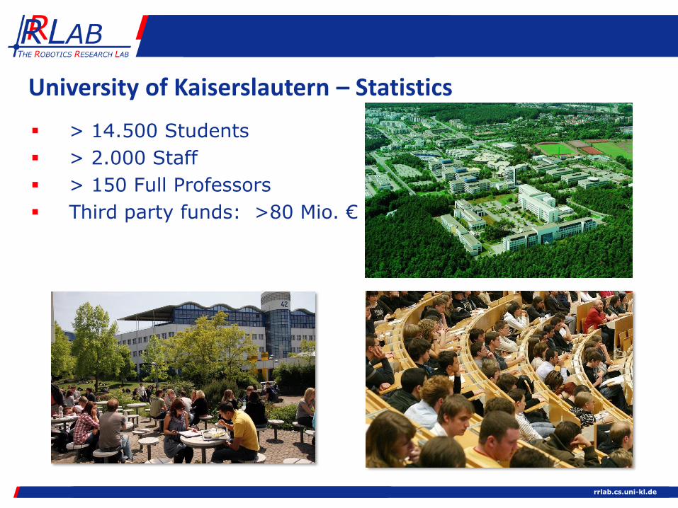
University of Kaiserslautern ndash Statistics
gt 14500 Students
gt 2000 Staff
gt 150 Full Professors
Third party funds gt80 Mio euro
rrlabcsuni-klde
Science Alliance Kaiserslautern
rrlabcsuni-klde
Scientific Researchers ~ 140
Technical Staff ~ 15
Professors 12
Senior Engineers 5
ZNT Statistics
Center for Commercial Vehicles Technology
rrlabcsuni-klde
Research at Robotics Research Lab (RRLab)
Methodology and Algorithms
Autonomous Mobile Robots
Hu
ma
no
id
Ro
bo
ts
Off-r
oa
d R
obo
ts
Serv
ic
e R
obo
ts
rrlabcsuni-klde
Off-road Projekte
BauwesenLandwirtschaftTest-Fahrzeuge Rescue Roboter
rrlabcsuni-klde
Autonomous Navigation of a Tractor - Windrow Guidance 18kmh
rrlabcsuni-klde
rrlabcsuni-klde
Contents
Modeling of Robots and Space
Vehicle Kinematics
Analytical Solution
Geometric Solution
Bicycle Model
Maneuverability of AMRs
Rigid Vehicle Dynamics
AMR ndash Modeling 9
rrlabcsuni-klde
Modeling of AMRs
and its Operational Environment
rrlabcsuni-kldeAMR ndash Modeling 11
Modeling of AMRs and the Operational Environment
Reduction of the robot complexityAMR movements as trajectories in a 3D Euclidian space
Objects are represented by boarder lines or geometric objects eg
polygon lines grids
boxes
AMR position can be
represented by a single
point in space
center of mass
kinematic center
Orientation (heading) represented as a vector due to the world frame
rrlabcsuni-kldeAMR ndash Modeling 12
Configuration Space
Configuration space (C-space) spanned over the degrees of freedom that should be considered
Eg a mobile robot in a 2D space contains all possible positions and orientations (119909 119910 120593) and maps each point to reachable or not reachable
2D robot C-space
rrlabcsuni-kldeAMR ndash Modeling 13
Configuration Space
Trajectory planning must take into account the AMR shape
=gt widened obstacles by the
reflected shape of the AMR
=gt if point representation
can reach a configuration the
same holds for the real robot
2D robot c-space
rrlabcsuni-kldeAMR ndash Modeling 14
Configuration Space
Extension of C-Space considering the derivatives of each degree of freedom
=gt Extension space (X-space)
Eg X-Space for considering velocity
Widen obstacles so that collision avoidance remainspossible (brakingdeceleration) 2D robot X-space
rrlabcsuni-klde
Coordinate Systems
AMR ndash Modeling 15
Modeling of a movement of an AMR by transformation of
the robot coordinate systems in a 3D Euclidian space
rrlabcsuni-kldeAMR ndash Modeling 16
Description of AMR Pose as Six-Tuple
In general the pose of an arbitrary object in the Cartesian space can be described as a six-tuple 119909 119910 119911 120593 120595 120579
The position vector 119874119906 in an object frame 119874 can be presented
in base frame coordinates 119861119906 by
119861119906 =119909119910119911
+ 119874119861119877 120593120595 120579 119874 119906
with 119909 119910 119911 119879 being the translation vector between the origin of the two frames and 119877 (3x3 matrix) the respective (combined) rotation matrix
rrlabcsuni-kldeAMR ndash Modeling 17
Homogeneous Transformation Matrix
Another possibility to express the same as above are homogeneous transformation matrices Those 4 times 4 matrices(for 3D space) are composed as shown below
119877 119906Ԧ119901119879 119904
119877 3 times 3 rotation (orientation) matrix
119906 Translation (position) - 119906 = 119906119909 119906119910 119906119911119879
Ԧ119901 Perspective transformation in general Ԧ119901 = 000 119879
119904 Scaling factor in general 119904 = 1
rrlabcsuni-kldeAMR ndash Modeling 18
3D Rotation Matrices
119877 is usually a combination of several rotations around the elementary axis
119877119909 120593 describes a rotation around the x-axis of an arbitrary coordinate system via the angle 120593 In an analog matter the other two required matrices are defined
119877119909 120593 =1 0 00 cos120593 minus sin1205930 sin120593 cos120593
119877119910 120595 =cos120595 0 sin1205950 1 0
minus sin120595 0 cos120595
119877119911 θ =cos θ minus sin θ 0sin θ cos θ 00 0 1 119909 119906
120593 119910
119907
119911119908
rrlabcsuni-kldeAMR ndash Modeling 19
Expression of Linked Rotations
Two possible ways of expressing linked rotations
Euler angles (rotation around variable axes)
119877 = 119877119911 120593 sdot 119877119909 120595 sdot 119877119911prime θ
Tait-Bryan angles ldquoRoll Pitch Yawrdquo (rotation around fixed axes)
119877 = 119877119911 θ sdot 119877119910 120595 sdot 119877119909 120593
rrlabcsuni-kldeAMR ndash Modeling 20
Roll Pitch Yaw
Euler rotations along ldquonewrdquo axes
Roll-Pitch-Yaw rotations along fixed axes
Terrestrial robotics the roll pitch yaw system is used (change of AMR pose according to world coordinate system)
Yaw θ
Pitchψ
Roll 120593
119911
119910119909
20
Roll
Pitch Yaw
119909
119911119910
rrlabcsuni-kldeAMR ndash Modeling 21
Combined Rotational Matrix (Roll Pitch Yaw)
Arbitrary orientation in 3D space can be described using three rotations
119877119904 as resulting matrix
(abbreviations 119904120593 for sin120593 and 119888120593 for cos120593)
119877119904 =
119888θ 119888120595 119888θ 119904120595 119904120593 minus 119904θ 119888120593 119888θ 119904120595 119888120593 + 119904θ 119904120593119904θ 119888120595 119904θ 119904120595 119904120593 + 119888θ 119888120593 119904θ 119904120595 119888120593 minus 119888θ 119904120593minus119904120595 119888120595 119904120593 119888120595 119888120593
rrlabcsuni-kldeAMR ndash Modeling 22
Linear Velocity
Transformation velocities between two frames is similar to pose transformation
Transformation of a linear velocity vector 119861 Ԧ119907119902 of an arbitrary
point Ԧ119902 presented in frame 119861 to frame 119860119860 Ԧ119907119902 = 119861
119860119877119861 Ԧ119907119902
If the origin of frame 119861 has also a linear velocity relative to frame 119860 then
119860 Ԧ119907119902 =119860 Ԧ119907119874119861 + 119861
119860119877119861 Ԧ119907119902
If in addition point Ԧ119902 is rotating around an arbitrary axis with
the rotational velocity 119860Ω119861 then the linear velocity can be
calculated with
119860 Ԧ119907119876 = 119860 Ԧ119907119874119861 + 119861119860119877119861 Ԧ119907119876 +
119860ω119861 times 119861119860119877119861 Ԧ119902
rrlabcsuni-kldeAMR ndash Modeling 23
Rotational Velocity
A rotational vector 119861120596 related to frame 119861 can be transferred
to frame 119860 with
119860120596 = 119861119860119877119861120596
rrlabcsuni-kldeAMR ndash Modeling 24
Linear and Rotational Velocity
Rotational and linear velocity of a sequence of segments connected by rotational or prismatic joints can stepwise be calculated
Rotational velocity 119894+1120596119894+1 and the linear velocity 119894+1 Ԧ119907119894+1relative to frame 119894 + 1 can be determined as
119894+1120596119894+1 = 119894119894+1119877 sdot 119894120596119894 + ሶθ119894+1
119894+1 Ԧ119890119911119894+1
119894+1 Ԧ119907119894+1 = 119894119894+1119877 119894 Ԧ119907119894 +
119894120596119894 times119894 Ԧ119901119894+1
with 119894 Ԧ119901119894+1 vector in direction of the segment 119894 120596119894 the rotational
velocity and 120595119894 the rotation of segment 119894 around the elementary 119911-axis
rrlabcsuni-kldeAMR ndash Modeling 25
Linear and Rotational Velocity
119894119894+1119877 is the inverse of the orientation matrix 119894+1
119894119877 from frame 119894 to
119894 + 1
119894+1119894119877 is an orthonormal matrix
its inverse 119894+1119894119877minus1 = 119894
119894+1119877 is the transposed matrix 119894+1119894119877119879
(example in 2D space)
119894119894+1119877 θ = 119894+1
119894119877minus1 θ = 119894+1119894119877119879 θ =
119888θ 119904θ 119909119908minus119904θ 119888θ 1199101199080 0 1
rrlabcsuni-klde
World (Global) and Robot (Local) Coordinate System
AMR ndash Modeling 26
YW
XW
θ
YR
XR
P
rrlabcsuni-kldeAMR ndash Modeling 27
World and Robot Coordinate System
119875 describes the location of the kinematic center relative to the world coordinate system
120579 is the mathematically positive angle between 119883119882 and 119883119877 119874 119883119882 119884119882 ෝ= origin of the world coordinate system
119874 119883119877 119884119877 ෝ= 119875 ෝ= origin of the robotrsquos coordinate system
119883119877-axis is longitudinal axis of the robot through its kinematic center
119884119877-axis is lateral axis of the robot through its kinematics center
120585119882 = 119909 119910 120579 119879 coordinates of the kineamtic center in world
coordinates
rrlabcsuni-kldeAMR ndash Modeling 28
World and Robot Coordinate System
Orientation via rotation around 119911-axis
119877 θ =cos θ sin θ 0minussin θ cos θ 0
0 0 1
Speed transformation from world- to robot coordinate system
ሶԦ120585119877 = 119877 θሶԦ120585119882
Coordinate transformation
YW
XW
θ
YR
XR
rrlabcsuni-kldeAMR ndash Modeling 29
World and Robot Coordinate System
Rotation around 119911-axis withθ = 90 deg
119877120587
2=
0 1 0minus1 0 00 0 1
Speed calculation in robot coordinates
ሶԦ120585119877 = 119877120587
2ሶ
120585119882 =0 1 0minus1 0 00 0 1
sdotሶ119909ሶ119910ሶθ
=ሶ119910
minus ሶ119909ሶθ
rrlabcsuni-klde
Vehicle Kinematics -
Analytical Solution
rrlabcsuni-kldeAMR ndash Kinematics 31
Control of the Test Vehicle GATOR
rrlabcsuni-kldeAMR ndash Kinematics 32
Forward kinematics for wheel driven robot
What is the robotrsquos trajectory if wheel geometry and speed are known
YW
XW
θ
V(t)
120596(t)
rrlabcsuni-kldeAMR ndash kinematics 33
Example Differential Drive
119903 radius of the wheel
119889 distance wheel center to kinematic center
ሶ120595119903 ሶ120595119897 Angular velocity of leftright wheel
ሶԦ120585119882 speed calculation in world coordinates
ሶԦ120585119882 = ሶ119909 ሶ119910 ሶ120579119879
= 119891 119889 119903 120579 ሶ120595119897 ሶ120595119903
= 119877 120579 minus1 ሶԦ120585119877
passive wheel
active wheel
d
rrlabcsuni-kldeAMR ndash Kinematics 34
Example Differential Drive
Calculation of the contribution of the left and right wheel to the speed along the longitudinal axis (119883119877)
Calculation of the contribution of the left and right wheel to the angular velocity of kinematic center
Summation of both results in the velocity and angular velocity along the 119883119877-axis where
ሶ119909119877119903 =119903 ሶ1205951199032
ሶ119909119877119897 =119903 ሶ120595119897
2
120596119903 =119903 ሶ1205951199032119889
120596119897 =minus119903 ሶ120595119897
2119889
ሶԦ120585119882 = 119877 120579 minus1 ሶԦ120585119903ሶԦ120585119903 =
119903 ሶ1205951199032
+119903 ሶ120595119897
2 0
119903 ሶ1205951199032119889
minus119903 ሶ120595119897
2119889
119879
rrlabcsuni-kldeAMR ndash Kinematics 35
Example Differential Drive
Since 119877 120579 is orthonormal
119877 120579 minus1 =cos 120579 minus sin 120579 0sin 120579 cos 120579 00 0 1
Given 120579 =120587
2 119903 = 1 119889 = 1 ሶ120595119903 = 4 ሶ120595119897 = 2 and wheel speed
notated in rounds per second 2120587
119904
ሶԦ120585119882 =ሶ119909ሶ119910ሶ120579
=0 minus1 01 0 00 0 1
sdot301
=031
rrlabcsuni-kldeAMR ndash Kinematics 36
Calculation of Wheel kinematics
Stepwise calculation of the linear and the rotational velocity for wheeled vehicles in 2D environment
Kinematic center moved with ሶ119909 ሶ119910 ሶ120579119879
Determine rotational velocity of each wheel
Collect all equations and solve the equation system
Consider
Equation system must no be solvable
No dynamic aspects will be considered
Calculation of the speed of the kinematic center based on thewheel speed can also be determined out of the equationsystem (inverse problem)
rrlabcsuni-klde
Basic Wheel Types
AMR ndash Kinematics 37
Standardwheel
Steerablestandard
wheel
Castorwheel
Swedish orMecanum
wheel
Ball orspherical
wheel
rrlabcsuni-kldeAMR ndash Kinematics 38
Wheel Properties
Standard and steerable wheel
Linear velocity along wheel plane ሶ119909 = 119903 ሶ120595
No sliding orthogonal to wheel plane ሶ119910 = 0
Castor wheel
Linear velocity along wheel plane ሶ119909 = 119903 ሶ120595
Linear perpendicular velocity ሶ119910 = minus119889119888 ሶ120573
SwedishMecanum wheel
Linear velocity along wheel plane ሶ119909 = 119903 ሶ120595 cos 120574
120574 angle of passive rollers (45 deg or 90 deg)
Linear perpendicular velocity ሶ119910 = 119903 ሶ120595 sin 120574 + 119903119901119903 ሶ120595119901119903
rrlabcsuni-kldeAMR ndash Kinematics 39
Kinematic Parameters
rrlabcsuni-kldeAMR ndash Kinematics 40
Kinematic Parameters
120572 Angle between 119909-axis and wheel mount point
120573 Angle between the straight line through the kinematic center and the fixing point of the wheel and the 119910-axis of the wheel frame
119889 Distance from the kinematic center to the wheel fixingpoint
119889119888 Distance from the wheel fixing point to the wheel supporting point (Castor wheel only)
120574 Angle between the 119909-axis of the wheel and rolling direction of the rollers (Mecanum wheel only)
rrlabcsuni-kldeAMR ndash Kinematics 41
Kinematic Parameters Standard Wheel
ሶ120595 119903
rrlabcsuni-kldeAMR ndash Kinematics 42
Kinematic Parameters Steerable Wheel
ሶ120595 119903
rrlabcsuni-kldeAMR ndash Kinematics 43
Kinematic Parameters Castor Wheel
ሶ120595 119903
rrlabcsuni-kldeAMR ndash Kinematics 44
Kinematic Parameters Mecanum Wheel
ሶ120595 119903
rrlabcsuni-kldeAMR ndash Kinematics 45
Kinematic Parameters Ball Wheel
ሶ120595 119903
rrlabcsuni-kldeAMR ndash Kinematics 46
Calculation of Wheel Velocity
Given velocity vector Ԧ119907 = ሶ119909 ሶ119910 ሶ120579119879
of the kinematic center
Calculation of linear velocity of standard wheel due to the speed of the kinematic center
Stepwise apply the following equations
Initial parameters 11205961 = 00 ሶ120579119879
and 1 Ԧ1199071 = ሶ119909 ሶ119910 0 119879
No additional rotational speed all 119894120596119894 = 00 ሶ120579119879
119894+1120596119894+1 = 119894119894+1119877 sdot 119894120596119894 + ሶ120579119894+1
119894+1 Ԧ119890119911119894+1
119894+1 Ԧ119907119894+1 = 119894119894+1119877 119894 Ԧ119907119894 +
119894120596119894 times119894 Ԧ119901119894+1
rrlabcsuni-kldeAMR ndash Kinematics 47
Calculation of Wheel Velocity
After the rotation around the 119911-axis with angle 120572 2 Ԧ1199072 is
calculated as
2 Ԧ1199072 =119888120572 ሶ119909 + 119904120572 ሶ119910minus119904120572 ሶ119909 + 119888120572 ሶ119910
0
Due to the translation 119889 3 Ԧ1199073 is
3 Ԧ1199073 =
119888120572 ሶ119909 + 119904120572 ሶ119910
minus119904120572 ሶ119909 + 119888120572 ሶ119910 + 119889 ሶ1205790
rrlabcsuni-kldeAMR ndash Kinematics 48
Calculation of Wheel Velocity
The last rotation around the 119911-axis with angle 120573 minus 90degtransfers the 119909-axis of the last frame to the rolling direction of the wheel
For the calculation of 4 Ԧ1199074 in the next equation
sin 120573 minus 90deg = minus cos120573 and cos 120573 minus 90deg = sin 120573 is used
4 Ԧ1199074 =119904 120572 + 120573 ሶ119909 minus 119888 120572 + 120573 ሶ119910 minus 119888120573 119889 ሶ120579
119888 120572 + 120573 ሶ119909 + 119904 120572 + 120573 ሶ119910 + 119904120573 119889 ሶ1205790
rrlabcsuni-kldeAMR ndash 4 Modeling 49
Calculation of Wheel Velocity
Last step is to equalize the linear velocity vector of the standard wheel to the velocity of the kinematic center represented in the wheel frame
119904 120572 + 120573 minus119888 120572 + 120573 minus119888120573 119889
119888 120572 + 120573 119904 120572 + 120573 119904120573 1198890 0 0
ሶ119909119910 ሶሶ120579
=119903 ሶ12059500
1st equation 119903 ሶ120595 = 119888 120572 + 120573 ሶ119909 + 119904 120572 + 120573 ሶ119910 + 119904120573 119889 ሶ120579 is called the
rolling constraint of the wheel because it describes the speed in the rolling direction of the wheel
2nd equation 119888 120572 + 120573 ሶ119909 + 119904 120572 + 120573 ሶ119910 + 119904120573 119889 ሶ120579 = 0 is called the
sliding constraint which describes the speed perpendicular to wheel plane
Sliding constraints are collected in Matrix 119878 ndash add row (119888(120572 +
rrlabcsuni-kldeAMR ndash Kinematics 50
Wheel Type-specific Velocity Vector
In case of the steerable standard wheel the fixed angle 120573 is replaced by a function 120573 119905
Equation could also be applied to the spherical wheel (based on the forces which affect the wheel and change 120573 119905 only a linear velocity in the rolling direction exists)
In case of castor wheels the y-component of the velocity
vector is depending on the angular velocity ሶ120573 and the length of the rod
119904 120572 + 120573(119905) minus119888 120572 + 120573(119905) minus119888120573(119905)119889
119888 120572 + 120573(119905) 119904 120572 + 120573(119905) 119904120573(119905)1198890 0 0
ሶ119909ሶ119910ሶ120579
=119903 ሶ120595
minus119889119888 ሶ120573(119905)0
Sliding constraints are collected in Matrix 119878 ndash add row 119888 120572 + 120573(119905) 119904 120572 + 120573(119905) 119904120573(119905)119889 (is used in section
maneuverability)
rrlabcsuni-kldeAMR ndash 4 Modeling 51
Wheel Type-specific Velocity Vector
Swedish or Mecanum wheel is able to move in an omnidirectional way
119904 120572 + 120573 + 120574 minus119888 120572 + 120573 + 120574 minus119888 120573 + 120574 119889
119888 120572 + 120573 + 120574 119904 120572 + 120573 + 120574 119904 120573 + 120574 1198890 0 0
ሶ119909ሶ119910ሶ120579
=119903 ሶ120595 cos 120574
119903 ሶ120595 sin 120574 + 119903119901119903 ሶ1205951199011199030
rrlabcsuni-kldeAMR ndash Kinematics 52
Vehicle Motion Calculation
Transformation of wheel velocities to velocity of kinematic center
Determine parameters 120572 120573 120574d indicating the wheel pose
Insert 120572 120573 120574 into appropriate wheel equation (as shown before) for each wheel
Solve system of equations
rrlabcsuni-kldeAMR ndash Kinematics 53
Differential Drive Kinematics
Two fixed standard wheels mounted on one axis
Kinematic center located in the middle of the axis
Distance between the kinematic center and each wheel 119889
Kinematic center is origin of coordinate frame
One solution for modeling the wheel configuration is to place the wheels on the 119910-axis
Kinematic parameters
120572119897 = 90 deg
120573119897 = 0 deg
120572119903 = minus90 deg
120573119903 = 180 deg
rrlabcsuni-kldeAMR ndash Kinematics 54
Differential Drive Kinematics
Apply equations for standard wheels (for the left and the right wheel)
119904 120572119897 + 120573119897 ሶ119909 minus 119888 120572119897 + 120573119897 ሶ119910 minus 119888120573119897 119889 ሶ120579 = 119903119897 ሶ120595119897
119888 120572119897 + 120573119897 ሶ119909 + 119904 120572119897 + 120573119897 ሶ119910 + 119904120573119897 119889 ሶ120579 = 0
119904 120572119903 + 120573119903 ሶ119909 minus 119888 120572119903 + 120573119903 ሶ119910 minus 119888120573119903 119889 ሶ120579 = 119903119903 ሶ120595119903119888 120572119903 + 120572119903 ሶ119909 + 119904 120572119903 + 120573119903 ሶ119910 + 119904120573119903 119889 ሶ120579 = 0
If the above mentioned parameters are inserted the following equations will result
ሶ119909 minus 119889 ሶ120579 = 119903119897 ሶ120595119897
ሶ119910 = 0
ሶ119909 + 119889 ሶ120579 = 119903119903 ሶ120595119903119910 = 0
rrlabcsuni-kldeAMR ndash Kinematics 55
Differential Drive Kinematics
Solving the system of equations yields
ሶ119909ሶ119910ሶ120579
=
1
2119903119897 ሶ120595119897 + 119903119903 ሶ120595119903
01
2119889minus119903119897 ሶ120595119897 + 119903119903 ሶ120595119903
rrlabcsuni-kldeAMR ndash Kinematics 56
Differential Drive Kinematics of MARVIN
rrlabcsuni-klde
CROMSCI ndash Equipped with 3 Steerable Standard Wheels
AMR ndash Kinematics 57
Climbing robot CROMSCI Wheel settings of CROMSCI
rrlabcsuni-klde
Omnidirectional Drive Kinematics
AMR ndash Kinematics 58
Typical orientations of the 3 steerable wheels of an omnidirectional vehicle
rrlabcsuni-kldeAMR ndash Kinematicsg 59
Omnidirectional Drive Kinematics
Three steerable standard wheels
Kinematic center located in the middle of the robot
Distance between the kinematic center and each wheel 119889
Origin of coordinates frame is kinematic center
Kinematic parameters
1205721 = 0 deg
1205722 = 120 deg
1205723 = minus120 deg
rrlabcsuni-kldeAMR ndash Kinematics 60
Omnidirectional Drive Kinematics
Applying equation for steerable standard wheel for each wheel leads to the following system of equations
119904 1205721 + 1205731 ሶ119909 minus 119888 1205721 + 1205731 ሶ119910 minus 119889 sdot 119888 1205731 ሶ120579 = 1199031 ሶ1205951
119904 1205722 + 1205732 ሶ119909 minus 119888 1205722 + 1205732 ሶ119910 minus 119889 sdot 119888 1205732 ሶ120579 = 1199032 ሶ1205952
119904 1205723 + 1205733 ሶ119909 minus 119888 1205723 + 1205733 ሶ119910 minus 119889 sdot 119888 1205733 ሶ120579 = 1199033 ሶ1205953
119888 1205721 + 1205731 ሶ119909 + 119904 1205721 + 1205731 ሶ119910 + 119889 sdot 119904 1205731 ሶ120579 = 0
119888 1205722 + 1205732 ሶ119909 + 119904 1205722 + 1205732 ሶ119910 + 119889 sdot 119904 1205732 ሶ120579 = 0
119888 1205723 + 1205733 ሶ119909 + 119904 1205723 + 1205733 ሶ119910 + 119889 sdot 119904 1205733 ሶ120579 = 0
rrlabcsuni-kldeAMR ndash Kinematics 61
Omnidirectional Drive Kinematics
Based on these equation the steering angles 120573119894 119894 = 123 can be determined
119888 120572119894 + 120573119894 sdot ሶ119909 + 119904 120572119894 + 120573119894 sdot ሶ119910 + 119889 sdot 119904 120573119894 sdot ሶ120579 = 0
119888 120572119894 sdot 119888 120573119894 sdot ሶ119909 minus 119904 120572119894 sdot 119904 120573119894 sdot ሶ119909 + 119904 120572119894 sdot 119888 120573119894 sdot ሶ119910 + 119888 120572119894 sdot 119904 120573119894 sdot ሶ119910 + 119889 sdot 119904 120573119894 sdot ሶ120579 = 0
119888 120573119894 sdot 119888 120572119894 sdot ሶ119909 + 119904 120572119894 sdot ሶ119910 minus 119904 120573119894 sdot 119904 120572119894 sdot ሶ119909 minus 119888 120572119894 sdot ሶ119910 minus 119889 sdot ሶ120579 = 0
119888 120572119894 sdot ሶ119909 + 119904 120572119894 sdot ሶ119910
119904 120572119894 sdot ሶ119909 minus 119888 120572119894 sdot ሶ119910 minus 119889 sdot ሶ120579=119904 120573119894119888 120573119894
atan2 119888 120572119894 sdot ሶ119909 + 119904 120572119894 sdot ሶ119910 119904 120572119894 sdot ሶ119909 minus 119888 120572119894 sdot ሶ119910 minus 119889 sdot ሶ120579 = 120573119894
Also the angular velocity of the wheel ሶ120595119894 can now be calculated
ሶ120595119894 =1
119903119894119904 120572119894 + 120573119894 ሶ119909 minus 119888 120572119894 + 120573119894 ሶ119910 minus 119889 sdot 119888 120573119894 ሶ120579
rrlabcsuni-klde
The Climbing Robot CROMSCI
AMR ndash Kinematics 62
rrlabcsuni-klde
Mecanum Vehicle
AMR ndash Kinematics 63
Schematic configurationof a Mecanum wheel(Viewed from above)
The mobile robot PRIAMOS of the University of Karlsruhe driven by Mecanum wheels
rrlabcsuni-kldeAMR ndash Kinematics 64
Mecanum Kinematics
To set up the kinematic equation first the parameters 120572 120573 120574for each wheel must be determined
The parameters for four wheels are
1205721 = 45 deg 1205731 = 45 deg 1205741 = minus45 deg
1205722 = 135 deg 1205732 = minus45 deg 1205742 = 45 deg
1205723 = minus135 deg 1205733 = 225 deg 1205743 = minus45 deg
1205724 = minus45 deg 1205734 = 135 deg 1205744 = 45 deg
rrlabcsuni-kldeAMR ndash Kinematics 65
Mecanum Kinematics
Assume all driven wheels have the same radius 119903 the same distance 119889 from the kinematic center and the above mentioned parameters 120572 120573 120574
Using equation for Mecanum wheels leads to equations
119904 45 deg ሶ119909 minus 119888 45 deg ሶ119910 minus 119889 ሶ120579 = 119903 sdot 119888 minus45 deg ሶ1205951
119904 135 deg ሶ119909 minus 119888 135 deg ሶ119910 minus 119889 ሶ120579 = 119903 sdot 119888 45 deg ሶ1205952
119904 45 deg ሶ119909 minus 119888 45 deg ሶ119910 minus 119889 ሶ120579 = 119903 sdot 119888 minus45 deg ሶ1205953
119904 135 deg ሶ119909 minus 119888 135 deg ሶ119910 minus 119889 ሶ120579 = 119903 sdot 119888 45 deg ሶ1205954
rrlabcsuni-kldeAMR ndash Kinematics 66
Mecanum Kinematics
The velocities ሶ119909 ሶ119910 ሶ120579 of the kinematic center can be calculated
ሶ119909 =119903
4ሶ1205951 + ሶ1205952 + ሶ1205953 + ሶ1205954
ሶ119910 =119903
4minus ሶ1205951 + ሶ1205952 minus ሶ1205953 + ሶ1205954
ሶ120579 =119903
119889 2ሶ1205951 minus ሶ1205952 minus ሶ1205953 + ሶ1205954
rrlabcsuni-kldeAMR ndash Kinematics 67
Mecanum Kinematics
The velocity vector of the kinematic center can be determined as
ሶ119909ሶ119910ሶ120579
=119903119908ℎ1198901198901198974
sdot1 1 1 1minus1 1 minus1 1119886 minus119886 minus119886 119886
sdot
ሶ1205951
ሶ1205952
ሶ1205953
ሶ1205954
with a =2 2
119889
Assuming the absence of slip the following must hold
ሶ1205954 = ሶ1205951 + ሶ1205952 minus ሶ1205953
rrlabcsuni-klde
Maneuverability of AMRs
rrlabcsuni-kldeAMR ndash Maneuverability 69
Choice of Wheel Configuration
Choice of wheels and their configuration depends on hellip
Ability to maneuver
Controllability
Stability
An optimum can only be achieved concerning a specific application
rrlabcsuni-kldeAMR ndash Maneuverability 70
Stability
Minimal number of wheels for static stability is 2 if center of gravity is located under the wheel axis (e g robot Cye)
Under standard conditions itrsquos 3
If more than 3 wheels are present adjustment to rough terrain becomes necessary
Typical setups
2 driven wheels on a single axis with 1 or 2 passive castor wheels
Single driven and steered wheel with two passive fixed wheels
rrlabcsuni-kldeAMR ndash Maneuverability 71
Maneuverability
Robotrsquos degree of freedom (DOF)
Outstanding ability to maneuver when the only driven wheel can be rotated in an active way
Example Ackermann steering
Poor ability to maneuver
5 m radius required for single rotation of a car
Lateral movement only possible troughforwardbackward movement
rrlabcsuni-kldeAMR ndash Maneuverability 72
Controllability
Costs for locomotion of the robot on a given trajectory
Contradiction to the robotrsquos ability to maneuver
Examples
Ackermann steering easy to control
Mecanum wheels very costly if high precision is required
Costs for controllability depend on hellip
Wheel type
Drive geometry
Sensors to determine driving situation
Motortransmission
rrlabcsuni-kldeAMR ndash Maneuverability 73
Degree of Mobility
The degree of mobility 119891119898 isin 123 points out how the sliding constraints (defined in Matrix 119878 see slide 42) affect the
possibilities for robot movement 119877 120579 ሶ120585119897 The mobility can be calculated by using the rank of the
matrix of sliding constraints of all standard wheels (steerable and fixed wheels) = number of independent constraints
119891119898 = 3 minus rank 119878
rrlabcsuni-kldeAMR ndash Maneuverability 74
Degree of Mobility
Example Differential Drive
Given only two fixed wheels geometrically we can set
1198891 = 1198892 1205731 = 1205732 = 0 1205721 + 120587 = 1205722
Matrix 119878 has two sliding constraints of the form (119888(120572 +
rrlabcsuni-kldeAMR ndash Maneuverability 75
Degree of Steerability
The degree of steerability 119891119904 isin 012 quantifies the degree of controllable freedom and is determined via the number of independently controllable steering parameters
Define 119878prime Part of 119878 defining sliding constraints of steerable wheels
119891119904 = rank 119878prime
More possibilities in steering will result in lower mobility
119891119904 = 0 No steered wheel (differential drive)
119891119904 = 1 At least one steered wheel (Ackermann steering)
119891119904 = 2 At least two steered wheels no fixed wheel
rrlabcsuni-kldeAMR ndash Maneuverability 76
Degree of Maneuverability
The degree of maneuverability 119891119872 isin 23 points out the number of DOF the robot can manipulate
119891119872 = 119891119898 + 119891119904
rrlabcsuni-klde
Vehicle Kinematics
Geometrical Solution
rrlabcsuni-kldeAMR ndash Kinematics 78
Tricycle Drive
Given 120575 119907
Unknown 119907prime 119907119897 119907119903 Solution
119903 = 119897 sdot cot 120575
119907prime =119907
cos 120575
119907119897 = 119907 sdot119903 + 119889
119903
119907119903 = 119907 sdot119903 minus 119889
119903 Tricycle drive kinematics
120575
rrlabcsuni-kldeAMR ndash 4 Kinematics 79
Ackermann Steering
Given 119907119863 120575 119897 119889
Unknown 119907119903119903 119907119897119903 119907119903119891 119907119897119891
Solution
120602 =119897
tan 120575
119907119897119903 =120602 minus 1198892 sdot 119907119863
120602
119907119903119903 =120602 + 1198892 sdot 119907119863
120602
119907119897119891 =120602 minus 1198892 2 + 1198972 sdot tan 120575
119897sdot 119907119863
119907119903119891 =1206022 + 1198972 sdot tan 120575
119897sdot 119907119863
Kinematics ofAckermann steering
120575
120602
rrlabcsuni-klde
Omnidrive Kinematics
AMR ndash Kinematics 80
Given 120602 120593 119907 119889
Unknown 1205931 1205932 1199071 1199072 Solution
120549119909 = 120602 sdot cos120593120549119910 = 120602 sdot sin1205931205931 = arctan120549119910 minus 1198891205491199091206021 = 120602 sdot cos120593 cos12059311199071 = 119907 sdot 1206021120602
1205932 = arctan120549119910 + 119889
1205491199091206022 = 120602 sdot cos120593 cos1205932
1199072 = 119907 sdot 1206022120602
120549119910 = 120602 ∙ 119904119894119899 120593
1205931
1205932
1206021
1206022
120593 120549119909 = 120602 ∙ cos120593
120602
119889
rrlabcsuni-klde
Bicycle Model
AMR ndash Kinematics 81
119907
rrlabcsuni-kldeAMR ndash Kinematics 82
Bicycle Model
Circular road of radius 120602
Low speed motion
Slip angles at both wheels are zero
Small total lateral force from both tires
119865119910 =1198981199072
120602
Point 119875 is instantaneous rolling center
Velocity at 119862 is perpendicular to line 119875119862
Heading angle 120579
Slip angle 120575119907 Course angle 120574 = 120579 + 120575119907
rrlabcsuni-kldeAMR ndash 4 Modeling 83
Bicycle Model
Given 120575119891 120575119903 119907 120579
Unknown ሶ119883 ሶ119884 ሶ120579
Solution
120575119907 = tanminus1119897119891 tan 120575119903+119897119903 tan 120575119891
119897119891+119897119903
ሶ120579 =119907
120602
120602 =119897119891+119897119903
tan 120575119891 minustan 120575119903 cos 120575119907
ሶ119883 = 119907 cos 120579 + 120575119907ሶ119884 = 119907 sin 120579 + 120575119907
ሶ120579 =119907 cos 120575119907
119897119891+119897119903tan 120575119891 minus tan 120575119903
119907
rrlabcsuni-klde
Ackermann Steering -gt Bicycle Model
AMR ndash Kinematics 84
119862 = 119874 120575119903 = 0 120575119891 = 120575
119897119903 = 0 119897119891 = 119897
120575119907 = 0
ሶ120579 =119907
120602
120602 =119897
tan 120575119891
ሶ119883 = 119907 cos 120579ሶ119884 = 119907 sin 120579ሶ120579 =
119907
119897119891tan 120575119891
119907

rrlabcsuni-klde
KaiserslauternGermany
Kaiserslautern
Frankfurt
Berlin
Hamburg
Bremen
Hanover
Cologne
Stuttgart
Munich
Braunschweig
Federal Republic of Germany
bull Deutschland
bull 16 constituent states
bull area of 357386 square
kilometres
bull (137988 sq mi)
bull 83 million inhabitants
bull Capital Berlin
(52deg31primeN 13deg23primeE)
rrlabcsuni-klde
University of Kaiserslautern ndash Statistics
gt 14500 Students
gt 2000 Staff
gt 150 Full Professors
Third party funds gt80 Mio euro
rrlabcsuni-klde
Science Alliance Kaiserslautern
rrlabcsuni-klde
Scientific Researchers ~ 140
Technical Staff ~ 15
Professors 12
Senior Engineers 5
ZNT Statistics
Center for Commercial Vehicles Technology
rrlabcsuni-klde
Research at Robotics Research Lab (RRLab)
Methodology and Algorithms
Autonomous Mobile Robots
Hu
ma
no
id
Ro
bo
ts
Off-r
oa
d R
obo
ts
Serv
ic
e R
obo
ts
rrlabcsuni-klde
Off-road Projekte
BauwesenLandwirtschaftTest-Fahrzeuge Rescue Roboter
rrlabcsuni-klde
Autonomous Navigation of a Tractor - Windrow Guidance 18kmh
rrlabcsuni-klde
rrlabcsuni-klde
Contents
Modeling of Robots and Space
Vehicle Kinematics
Analytical Solution
Geometric Solution
Bicycle Model
Maneuverability of AMRs
Rigid Vehicle Dynamics
AMR ndash Modeling 9
rrlabcsuni-klde
Modeling of AMRs
and its Operational Environment
rrlabcsuni-kldeAMR ndash Modeling 11
Modeling of AMRs and the Operational Environment
Reduction of the robot complexityAMR movements as trajectories in a 3D Euclidian space
Objects are represented by boarder lines or geometric objects eg
polygon lines grids
boxes
AMR position can be
represented by a single
point in space
center of mass
kinematic center
Orientation (heading) represented as a vector due to the world frame
rrlabcsuni-kldeAMR ndash Modeling 12
Configuration Space
Configuration space (C-space) spanned over the degrees of freedom that should be considered
Eg a mobile robot in a 2D space contains all possible positions and orientations (119909 119910 120593) and maps each point to reachable or not reachable
2D robot C-space
rrlabcsuni-kldeAMR ndash Modeling 13
Configuration Space
Trajectory planning must take into account the AMR shape
=gt widened obstacles by the
reflected shape of the AMR
=gt if point representation
can reach a configuration the
same holds for the real robot
2D robot c-space
rrlabcsuni-kldeAMR ndash Modeling 14
Configuration Space
Extension of C-Space considering the derivatives of each degree of freedom
=gt Extension space (X-space)
Eg X-Space for considering velocity
Widen obstacles so that collision avoidance remainspossible (brakingdeceleration) 2D robot X-space
rrlabcsuni-klde
Coordinate Systems
AMR ndash Modeling 15
Modeling of a movement of an AMR by transformation of
the robot coordinate systems in a 3D Euclidian space
rrlabcsuni-kldeAMR ndash Modeling 16
Description of AMR Pose as Six-Tuple
In general the pose of an arbitrary object in the Cartesian space can be described as a six-tuple 119909 119910 119911 120593 120595 120579
The position vector 119874119906 in an object frame 119874 can be presented
in base frame coordinates 119861119906 by
119861119906 =119909119910119911
+ 119874119861119877 120593120595 120579 119874 119906
with 119909 119910 119911 119879 being the translation vector between the origin of the two frames and 119877 (3x3 matrix) the respective (combined) rotation matrix
rrlabcsuni-kldeAMR ndash Modeling 17
Homogeneous Transformation Matrix
Another possibility to express the same as above are homogeneous transformation matrices Those 4 times 4 matrices(for 3D space) are composed as shown below
119877 119906Ԧ119901119879 119904
119877 3 times 3 rotation (orientation) matrix
119906 Translation (position) - 119906 = 119906119909 119906119910 119906119911119879
Ԧ119901 Perspective transformation in general Ԧ119901 = 000 119879
119904 Scaling factor in general 119904 = 1
rrlabcsuni-kldeAMR ndash Modeling 18
3D Rotation Matrices
119877 is usually a combination of several rotations around the elementary axis
119877119909 120593 describes a rotation around the x-axis of an arbitrary coordinate system via the angle 120593 In an analog matter the other two required matrices are defined
119877119909 120593 =1 0 00 cos120593 minus sin1205930 sin120593 cos120593
119877119910 120595 =cos120595 0 sin1205950 1 0
minus sin120595 0 cos120595
119877119911 θ =cos θ minus sin θ 0sin θ cos θ 00 0 1 119909 119906
120593 119910
119907
119911119908
rrlabcsuni-kldeAMR ndash Modeling 19
Expression of Linked Rotations
Two possible ways of expressing linked rotations
Euler angles (rotation around variable axes)
119877 = 119877119911 120593 sdot 119877119909 120595 sdot 119877119911prime θ
Tait-Bryan angles ldquoRoll Pitch Yawrdquo (rotation around fixed axes)
119877 = 119877119911 θ sdot 119877119910 120595 sdot 119877119909 120593
rrlabcsuni-kldeAMR ndash Modeling 20
Roll Pitch Yaw
Euler rotations along ldquonewrdquo axes
Roll-Pitch-Yaw rotations along fixed axes
Terrestrial robotics the roll pitch yaw system is used (change of AMR pose according to world coordinate system)
Yaw θ
Pitchψ
Roll 120593
119911
119910119909
20
Roll
Pitch Yaw
119909
119911119910
rrlabcsuni-kldeAMR ndash Modeling 21
Combined Rotational Matrix (Roll Pitch Yaw)
Arbitrary orientation in 3D space can be described using three rotations
119877119904 as resulting matrix
(abbreviations 119904120593 for sin120593 and 119888120593 for cos120593)
119877119904 =
119888θ 119888120595 119888θ 119904120595 119904120593 minus 119904θ 119888120593 119888θ 119904120595 119888120593 + 119904θ 119904120593119904θ 119888120595 119904θ 119904120595 119904120593 + 119888θ 119888120593 119904θ 119904120595 119888120593 minus 119888θ 119904120593minus119904120595 119888120595 119904120593 119888120595 119888120593
rrlabcsuni-kldeAMR ndash Modeling 22
Linear Velocity
Transformation velocities between two frames is similar to pose transformation
Transformation of a linear velocity vector 119861 Ԧ119907119902 of an arbitrary
point Ԧ119902 presented in frame 119861 to frame 119860119860 Ԧ119907119902 = 119861
119860119877119861 Ԧ119907119902
If the origin of frame 119861 has also a linear velocity relative to frame 119860 then
119860 Ԧ119907119902 =119860 Ԧ119907119874119861 + 119861
119860119877119861 Ԧ119907119902
If in addition point Ԧ119902 is rotating around an arbitrary axis with
the rotational velocity 119860Ω119861 then the linear velocity can be
calculated with
119860 Ԧ119907119876 = 119860 Ԧ119907119874119861 + 119861119860119877119861 Ԧ119907119876 +
119860ω119861 times 119861119860119877119861 Ԧ119902
rrlabcsuni-kldeAMR ndash Modeling 23
Rotational Velocity
A rotational vector 119861120596 related to frame 119861 can be transferred
to frame 119860 with
119860120596 = 119861119860119877119861120596
rrlabcsuni-kldeAMR ndash Modeling 24
Linear and Rotational Velocity
Rotational and linear velocity of a sequence of segments connected by rotational or prismatic joints can stepwise be calculated
Rotational velocity 119894+1120596119894+1 and the linear velocity 119894+1 Ԧ119907119894+1relative to frame 119894 + 1 can be determined as
119894+1120596119894+1 = 119894119894+1119877 sdot 119894120596119894 + ሶθ119894+1
119894+1 Ԧ119890119911119894+1
119894+1 Ԧ119907119894+1 = 119894119894+1119877 119894 Ԧ119907119894 +
119894120596119894 times119894 Ԧ119901119894+1
with 119894 Ԧ119901119894+1 vector in direction of the segment 119894 120596119894 the rotational
velocity and 120595119894 the rotation of segment 119894 around the elementary 119911-axis
rrlabcsuni-kldeAMR ndash Modeling 25
Linear and Rotational Velocity
119894119894+1119877 is the inverse of the orientation matrix 119894+1
119894119877 from frame 119894 to
119894 + 1
119894+1119894119877 is an orthonormal matrix
its inverse 119894+1119894119877minus1 = 119894
119894+1119877 is the transposed matrix 119894+1119894119877119879
(example in 2D space)
119894119894+1119877 θ = 119894+1
119894119877minus1 θ = 119894+1119894119877119879 θ =
119888θ 119904θ 119909119908minus119904θ 119888θ 1199101199080 0 1
rrlabcsuni-klde
World (Global) and Robot (Local) Coordinate System
AMR ndash Modeling 26
YW
XW
θ
YR
XR
P
rrlabcsuni-kldeAMR ndash Modeling 27
World and Robot Coordinate System
119875 describes the location of the kinematic center relative to the world coordinate system
120579 is the mathematically positive angle between 119883119882 and 119883119877 119874 119883119882 119884119882 ෝ= origin of the world coordinate system
119874 119883119877 119884119877 ෝ= 119875 ෝ= origin of the robotrsquos coordinate system
119883119877-axis is longitudinal axis of the robot through its kinematic center
119884119877-axis is lateral axis of the robot through its kinematics center
120585119882 = 119909 119910 120579 119879 coordinates of the kineamtic center in world
coordinates
rrlabcsuni-kldeAMR ndash Modeling 28
World and Robot Coordinate System
Orientation via rotation around 119911-axis
119877 θ =cos θ sin θ 0minussin θ cos θ 0
0 0 1
Speed transformation from world- to robot coordinate system
ሶԦ120585119877 = 119877 θሶԦ120585119882
Coordinate transformation
YW
XW
θ
YR
XR
rrlabcsuni-kldeAMR ndash Modeling 29
World and Robot Coordinate System
Rotation around 119911-axis withθ = 90 deg
119877120587
2=
0 1 0minus1 0 00 0 1
Speed calculation in robot coordinates
ሶԦ120585119877 = 119877120587
2ሶ
120585119882 =0 1 0minus1 0 00 0 1
sdotሶ119909ሶ119910ሶθ
=ሶ119910
minus ሶ119909ሶθ
rrlabcsuni-klde
Vehicle Kinematics -
Analytical Solution
rrlabcsuni-kldeAMR ndash Kinematics 31
Control of the Test Vehicle GATOR
rrlabcsuni-kldeAMR ndash Kinematics 32
Forward kinematics for wheel driven robot
What is the robotrsquos trajectory if wheel geometry and speed are known
YW
XW
θ
V(t)
120596(t)
rrlabcsuni-kldeAMR ndash kinematics 33
Example Differential Drive
119903 radius of the wheel
119889 distance wheel center to kinematic center
ሶ120595119903 ሶ120595119897 Angular velocity of leftright wheel
ሶԦ120585119882 speed calculation in world coordinates
ሶԦ120585119882 = ሶ119909 ሶ119910 ሶ120579119879
= 119891 119889 119903 120579 ሶ120595119897 ሶ120595119903
= 119877 120579 minus1 ሶԦ120585119877
passive wheel
active wheel
d
rrlabcsuni-kldeAMR ndash Kinematics 34
Example Differential Drive
Calculation of the contribution of the left and right wheel to the speed along the longitudinal axis (119883119877)
Calculation of the contribution of the left and right wheel to the angular velocity of kinematic center
Summation of both results in the velocity and angular velocity along the 119883119877-axis where
ሶ119909119877119903 =119903 ሶ1205951199032
ሶ119909119877119897 =119903 ሶ120595119897
2
120596119903 =119903 ሶ1205951199032119889
120596119897 =minus119903 ሶ120595119897
2119889
ሶԦ120585119882 = 119877 120579 minus1 ሶԦ120585119903ሶԦ120585119903 =
119903 ሶ1205951199032
+119903 ሶ120595119897
2 0
119903 ሶ1205951199032119889
minus119903 ሶ120595119897
2119889
119879
rrlabcsuni-kldeAMR ndash Kinematics 35
Example Differential Drive
Since 119877 120579 is orthonormal
119877 120579 minus1 =cos 120579 minus sin 120579 0sin 120579 cos 120579 00 0 1
Given 120579 =120587
2 119903 = 1 119889 = 1 ሶ120595119903 = 4 ሶ120595119897 = 2 and wheel speed
notated in rounds per second 2120587
119904
ሶԦ120585119882 =ሶ119909ሶ119910ሶ120579
=0 minus1 01 0 00 0 1
sdot301
=031
rrlabcsuni-kldeAMR ndash Kinematics 36
Calculation of Wheel kinematics
Stepwise calculation of the linear and the rotational velocity for wheeled vehicles in 2D environment
Kinematic center moved with ሶ119909 ሶ119910 ሶ120579119879
Determine rotational velocity of each wheel
Collect all equations and solve the equation system
Consider
Equation system must no be solvable
No dynamic aspects will be considered
Calculation of the speed of the kinematic center based on thewheel speed can also be determined out of the equationsystem (inverse problem)
rrlabcsuni-klde
Basic Wheel Types
AMR ndash Kinematics 37
Standardwheel
Steerablestandard
wheel
Castorwheel
Swedish orMecanum
wheel
Ball orspherical
wheel
rrlabcsuni-kldeAMR ndash Kinematics 38
Wheel Properties
Standard and steerable wheel
Linear velocity along wheel plane ሶ119909 = 119903 ሶ120595
No sliding orthogonal to wheel plane ሶ119910 = 0
Castor wheel
Linear velocity along wheel plane ሶ119909 = 119903 ሶ120595
Linear perpendicular velocity ሶ119910 = minus119889119888 ሶ120573
SwedishMecanum wheel
Linear velocity along wheel plane ሶ119909 = 119903 ሶ120595 cos 120574
120574 angle of passive rollers (45 deg or 90 deg)
Linear perpendicular velocity ሶ119910 = 119903 ሶ120595 sin 120574 + 119903119901119903 ሶ120595119901119903
rrlabcsuni-kldeAMR ndash Kinematics 39
Kinematic Parameters
rrlabcsuni-kldeAMR ndash Kinematics 40
Kinematic Parameters
120572 Angle between 119909-axis and wheel mount point
120573 Angle between the straight line through the kinematic center and the fixing point of the wheel and the 119910-axis of the wheel frame
119889 Distance from the kinematic center to the wheel fixingpoint
119889119888 Distance from the wheel fixing point to the wheel supporting point (Castor wheel only)
120574 Angle between the 119909-axis of the wheel and rolling direction of the rollers (Mecanum wheel only)
rrlabcsuni-kldeAMR ndash Kinematics 41
Kinematic Parameters Standard Wheel
ሶ120595 119903
rrlabcsuni-kldeAMR ndash Kinematics 42
Kinematic Parameters Steerable Wheel
ሶ120595 119903
rrlabcsuni-kldeAMR ndash Kinematics 43
Kinematic Parameters Castor Wheel
ሶ120595 119903
rrlabcsuni-kldeAMR ndash Kinematics 44
Kinematic Parameters Mecanum Wheel
ሶ120595 119903
rrlabcsuni-kldeAMR ndash Kinematics 45
Kinematic Parameters Ball Wheel
ሶ120595 119903
rrlabcsuni-kldeAMR ndash Kinematics 46
Calculation of Wheel Velocity
Given velocity vector Ԧ119907 = ሶ119909 ሶ119910 ሶ120579119879
of the kinematic center
Calculation of linear velocity of standard wheel due to the speed of the kinematic center
Stepwise apply the following equations
Initial parameters 11205961 = 00 ሶ120579119879
and 1 Ԧ1199071 = ሶ119909 ሶ119910 0 119879
No additional rotational speed all 119894120596119894 = 00 ሶ120579119879
119894+1120596119894+1 = 119894119894+1119877 sdot 119894120596119894 + ሶ120579119894+1
119894+1 Ԧ119890119911119894+1
119894+1 Ԧ119907119894+1 = 119894119894+1119877 119894 Ԧ119907119894 +
119894120596119894 times119894 Ԧ119901119894+1
rrlabcsuni-kldeAMR ndash Kinematics 47
Calculation of Wheel Velocity
After the rotation around the 119911-axis with angle 120572 2 Ԧ1199072 is
calculated as
2 Ԧ1199072 =119888120572 ሶ119909 + 119904120572 ሶ119910minus119904120572 ሶ119909 + 119888120572 ሶ119910
0
Due to the translation 119889 3 Ԧ1199073 is
3 Ԧ1199073 =
119888120572 ሶ119909 + 119904120572 ሶ119910
minus119904120572 ሶ119909 + 119888120572 ሶ119910 + 119889 ሶ1205790
rrlabcsuni-kldeAMR ndash Kinematics 48
Calculation of Wheel Velocity
The last rotation around the 119911-axis with angle 120573 minus 90degtransfers the 119909-axis of the last frame to the rolling direction of the wheel
For the calculation of 4 Ԧ1199074 in the next equation
sin 120573 minus 90deg = minus cos120573 and cos 120573 minus 90deg = sin 120573 is used
4 Ԧ1199074 =119904 120572 + 120573 ሶ119909 minus 119888 120572 + 120573 ሶ119910 minus 119888120573 119889 ሶ120579
119888 120572 + 120573 ሶ119909 + 119904 120572 + 120573 ሶ119910 + 119904120573 119889 ሶ1205790
rrlabcsuni-kldeAMR ndash 4 Modeling 49
Calculation of Wheel Velocity
Last step is to equalize the linear velocity vector of the standard wheel to the velocity of the kinematic center represented in the wheel frame
119904 120572 + 120573 minus119888 120572 + 120573 minus119888120573 119889
119888 120572 + 120573 119904 120572 + 120573 119904120573 1198890 0 0
ሶ119909119910 ሶሶ120579
=119903 ሶ12059500
1st equation 119903 ሶ120595 = 119888 120572 + 120573 ሶ119909 + 119904 120572 + 120573 ሶ119910 + 119904120573 119889 ሶ120579 is called the
rolling constraint of the wheel because it describes the speed in the rolling direction of the wheel
2nd equation 119888 120572 + 120573 ሶ119909 + 119904 120572 + 120573 ሶ119910 + 119904120573 119889 ሶ120579 = 0 is called the
sliding constraint which describes the speed perpendicular to wheel plane
Sliding constraints are collected in Matrix 119878 ndash add row (119888(120572 +
rrlabcsuni-kldeAMR ndash Kinematics 50
Wheel Type-specific Velocity Vector
In case of the steerable standard wheel the fixed angle 120573 is replaced by a function 120573 119905
Equation could also be applied to the spherical wheel (based on the forces which affect the wheel and change 120573 119905 only a linear velocity in the rolling direction exists)
In case of castor wheels the y-component of the velocity
vector is depending on the angular velocity ሶ120573 and the length of the rod
119904 120572 + 120573(119905) minus119888 120572 + 120573(119905) minus119888120573(119905)119889
119888 120572 + 120573(119905) 119904 120572 + 120573(119905) 119904120573(119905)1198890 0 0
ሶ119909ሶ119910ሶ120579
=119903 ሶ120595
minus119889119888 ሶ120573(119905)0
Sliding constraints are collected in Matrix 119878 ndash add row 119888 120572 + 120573(119905) 119904 120572 + 120573(119905) 119904120573(119905)119889 (is used in section
maneuverability)
rrlabcsuni-kldeAMR ndash 4 Modeling 51
Wheel Type-specific Velocity Vector
Swedish or Mecanum wheel is able to move in an omnidirectional way
119904 120572 + 120573 + 120574 minus119888 120572 + 120573 + 120574 minus119888 120573 + 120574 119889
119888 120572 + 120573 + 120574 119904 120572 + 120573 + 120574 119904 120573 + 120574 1198890 0 0
ሶ119909ሶ119910ሶ120579
=119903 ሶ120595 cos 120574
119903 ሶ120595 sin 120574 + 119903119901119903 ሶ1205951199011199030
rrlabcsuni-kldeAMR ndash Kinematics 52
Vehicle Motion Calculation
Transformation of wheel velocities to velocity of kinematic center
Determine parameters 120572 120573 120574d indicating the wheel pose
Insert 120572 120573 120574 into appropriate wheel equation (as shown before) for each wheel
Solve system of equations
rrlabcsuni-kldeAMR ndash Kinematics 53
Differential Drive Kinematics
Two fixed standard wheels mounted on one axis
Kinematic center located in the middle of the axis
Distance between the kinematic center and each wheel 119889
Kinematic center is origin of coordinate frame
One solution for modeling the wheel configuration is to place the wheels on the 119910-axis
Kinematic parameters
120572119897 = 90 deg
120573119897 = 0 deg
120572119903 = minus90 deg
120573119903 = 180 deg
rrlabcsuni-kldeAMR ndash Kinematics 54
Differential Drive Kinematics
Apply equations for standard wheels (for the left and the right wheel)
119904 120572119897 + 120573119897 ሶ119909 minus 119888 120572119897 + 120573119897 ሶ119910 minus 119888120573119897 119889 ሶ120579 = 119903119897 ሶ120595119897
119888 120572119897 + 120573119897 ሶ119909 + 119904 120572119897 + 120573119897 ሶ119910 + 119904120573119897 119889 ሶ120579 = 0
119904 120572119903 + 120573119903 ሶ119909 minus 119888 120572119903 + 120573119903 ሶ119910 minus 119888120573119903 119889 ሶ120579 = 119903119903 ሶ120595119903119888 120572119903 + 120572119903 ሶ119909 + 119904 120572119903 + 120573119903 ሶ119910 + 119904120573119903 119889 ሶ120579 = 0
If the above mentioned parameters are inserted the following equations will result
ሶ119909 minus 119889 ሶ120579 = 119903119897 ሶ120595119897
ሶ119910 = 0
ሶ119909 + 119889 ሶ120579 = 119903119903 ሶ120595119903119910 = 0
rrlabcsuni-kldeAMR ndash Kinematics 55
Differential Drive Kinematics
Solving the system of equations yields
ሶ119909ሶ119910ሶ120579
=
1
2119903119897 ሶ120595119897 + 119903119903 ሶ120595119903
01
2119889minus119903119897 ሶ120595119897 + 119903119903 ሶ120595119903
rrlabcsuni-kldeAMR ndash Kinematics 56
Differential Drive Kinematics of MARVIN
rrlabcsuni-klde
CROMSCI ndash Equipped with 3 Steerable Standard Wheels
AMR ndash Kinematics 57
Climbing robot CROMSCI Wheel settings of CROMSCI
rrlabcsuni-klde
Omnidirectional Drive Kinematics
AMR ndash Kinematics 58
Typical orientations of the 3 steerable wheels of an omnidirectional vehicle
rrlabcsuni-kldeAMR ndash Kinematicsg 59
Omnidirectional Drive Kinematics
Three steerable standard wheels
Kinematic center located in the middle of the robot
Distance between the kinematic center and each wheel 119889
Origin of coordinates frame is kinematic center
Kinematic parameters
1205721 = 0 deg
1205722 = 120 deg
1205723 = minus120 deg
rrlabcsuni-kldeAMR ndash Kinematics 60
Omnidirectional Drive Kinematics
Applying equation for steerable standard wheel for each wheel leads to the following system of equations
119904 1205721 + 1205731 ሶ119909 minus 119888 1205721 + 1205731 ሶ119910 minus 119889 sdot 119888 1205731 ሶ120579 = 1199031 ሶ1205951
119904 1205722 + 1205732 ሶ119909 minus 119888 1205722 + 1205732 ሶ119910 minus 119889 sdot 119888 1205732 ሶ120579 = 1199032 ሶ1205952
119904 1205723 + 1205733 ሶ119909 minus 119888 1205723 + 1205733 ሶ119910 minus 119889 sdot 119888 1205733 ሶ120579 = 1199033 ሶ1205953
119888 1205721 + 1205731 ሶ119909 + 119904 1205721 + 1205731 ሶ119910 + 119889 sdot 119904 1205731 ሶ120579 = 0
119888 1205722 + 1205732 ሶ119909 + 119904 1205722 + 1205732 ሶ119910 + 119889 sdot 119904 1205732 ሶ120579 = 0
119888 1205723 + 1205733 ሶ119909 + 119904 1205723 + 1205733 ሶ119910 + 119889 sdot 119904 1205733 ሶ120579 = 0
rrlabcsuni-kldeAMR ndash Kinematics 61
Omnidirectional Drive Kinematics
Based on these equation the steering angles 120573119894 119894 = 123 can be determined
119888 120572119894 + 120573119894 sdot ሶ119909 + 119904 120572119894 + 120573119894 sdot ሶ119910 + 119889 sdot 119904 120573119894 sdot ሶ120579 = 0
119888 120572119894 sdot 119888 120573119894 sdot ሶ119909 minus 119904 120572119894 sdot 119904 120573119894 sdot ሶ119909 + 119904 120572119894 sdot 119888 120573119894 sdot ሶ119910 + 119888 120572119894 sdot 119904 120573119894 sdot ሶ119910 + 119889 sdot 119904 120573119894 sdot ሶ120579 = 0
119888 120573119894 sdot 119888 120572119894 sdot ሶ119909 + 119904 120572119894 sdot ሶ119910 minus 119904 120573119894 sdot 119904 120572119894 sdot ሶ119909 minus 119888 120572119894 sdot ሶ119910 minus 119889 sdot ሶ120579 = 0
119888 120572119894 sdot ሶ119909 + 119904 120572119894 sdot ሶ119910
119904 120572119894 sdot ሶ119909 minus 119888 120572119894 sdot ሶ119910 minus 119889 sdot ሶ120579=119904 120573119894119888 120573119894
atan2 119888 120572119894 sdot ሶ119909 + 119904 120572119894 sdot ሶ119910 119904 120572119894 sdot ሶ119909 minus 119888 120572119894 sdot ሶ119910 minus 119889 sdot ሶ120579 = 120573119894
Also the angular velocity of the wheel ሶ120595119894 can now be calculated
ሶ120595119894 =1
119903119894119904 120572119894 + 120573119894 ሶ119909 minus 119888 120572119894 + 120573119894 ሶ119910 minus 119889 sdot 119888 120573119894 ሶ120579
rrlabcsuni-klde
The Climbing Robot CROMSCI
AMR ndash Kinematics 62
rrlabcsuni-klde
Mecanum Vehicle
AMR ndash Kinematics 63
Schematic configurationof a Mecanum wheel(Viewed from above)
The mobile robot PRIAMOS of the University of Karlsruhe driven by Mecanum wheels
rrlabcsuni-kldeAMR ndash Kinematics 64
Mecanum Kinematics
To set up the kinematic equation first the parameters 120572 120573 120574for each wheel must be determined
The parameters for four wheels are
1205721 = 45 deg 1205731 = 45 deg 1205741 = minus45 deg
1205722 = 135 deg 1205732 = minus45 deg 1205742 = 45 deg
1205723 = minus135 deg 1205733 = 225 deg 1205743 = minus45 deg
1205724 = minus45 deg 1205734 = 135 deg 1205744 = 45 deg
rrlabcsuni-kldeAMR ndash Kinematics 65
Mecanum Kinematics
Assume all driven wheels have the same radius 119903 the same distance 119889 from the kinematic center and the above mentioned parameters 120572 120573 120574
Using equation for Mecanum wheels leads to equations
119904 45 deg ሶ119909 minus 119888 45 deg ሶ119910 minus 119889 ሶ120579 = 119903 sdot 119888 minus45 deg ሶ1205951
119904 135 deg ሶ119909 minus 119888 135 deg ሶ119910 minus 119889 ሶ120579 = 119903 sdot 119888 45 deg ሶ1205952
119904 45 deg ሶ119909 minus 119888 45 deg ሶ119910 minus 119889 ሶ120579 = 119903 sdot 119888 minus45 deg ሶ1205953
119904 135 deg ሶ119909 minus 119888 135 deg ሶ119910 minus 119889 ሶ120579 = 119903 sdot 119888 45 deg ሶ1205954
rrlabcsuni-kldeAMR ndash Kinematics 66
Mecanum Kinematics
The velocities ሶ119909 ሶ119910 ሶ120579 of the kinematic center can be calculated
ሶ119909 =119903
4ሶ1205951 + ሶ1205952 + ሶ1205953 + ሶ1205954
ሶ119910 =119903
4minus ሶ1205951 + ሶ1205952 minus ሶ1205953 + ሶ1205954
ሶ120579 =119903
119889 2ሶ1205951 minus ሶ1205952 minus ሶ1205953 + ሶ1205954
rrlabcsuni-kldeAMR ndash Kinematics 67
Mecanum Kinematics
The velocity vector of the kinematic center can be determined as
ሶ119909ሶ119910ሶ120579
=119903119908ℎ1198901198901198974
sdot1 1 1 1minus1 1 minus1 1119886 minus119886 minus119886 119886
sdot
ሶ1205951
ሶ1205952
ሶ1205953
ሶ1205954
with a =2 2
119889
Assuming the absence of slip the following must hold
ሶ1205954 = ሶ1205951 + ሶ1205952 minus ሶ1205953
rrlabcsuni-klde
Maneuverability of AMRs
rrlabcsuni-kldeAMR ndash Maneuverability 69
Choice of Wheel Configuration
Choice of wheels and their configuration depends on hellip
Ability to maneuver
Controllability
Stability
An optimum can only be achieved concerning a specific application
rrlabcsuni-kldeAMR ndash Maneuverability 70
Stability
Minimal number of wheels for static stability is 2 if center of gravity is located under the wheel axis (e g robot Cye)
Under standard conditions itrsquos 3
If more than 3 wheels are present adjustment to rough terrain becomes necessary
Typical setups
2 driven wheels on a single axis with 1 or 2 passive castor wheels
Single driven and steered wheel with two passive fixed wheels
rrlabcsuni-kldeAMR ndash Maneuverability 71
Maneuverability
Robotrsquos degree of freedom (DOF)
Outstanding ability to maneuver when the only driven wheel can be rotated in an active way
Example Ackermann steering
Poor ability to maneuver
5 m radius required for single rotation of a car
Lateral movement only possible troughforwardbackward movement
rrlabcsuni-kldeAMR ndash Maneuverability 72
Controllability
Costs for locomotion of the robot on a given trajectory
Contradiction to the robotrsquos ability to maneuver
Examples
Ackermann steering easy to control
Mecanum wheels very costly if high precision is required
Costs for controllability depend on hellip
Wheel type
Drive geometry
Sensors to determine driving situation
Motortransmission
rrlabcsuni-kldeAMR ndash Maneuverability 73
Degree of Mobility
The degree of mobility 119891119898 isin 123 points out how the sliding constraints (defined in Matrix 119878 see slide 42) affect the
possibilities for robot movement 119877 120579 ሶ120585119897 The mobility can be calculated by using the rank of the
matrix of sliding constraints of all standard wheels (steerable and fixed wheels) = number of independent constraints
119891119898 = 3 minus rank 119878
rrlabcsuni-kldeAMR ndash Maneuverability 74
Degree of Mobility
Example Differential Drive
Given only two fixed wheels geometrically we can set
1198891 = 1198892 1205731 = 1205732 = 0 1205721 + 120587 = 1205722
Matrix 119878 has two sliding constraints of the form (119888(120572 +
rrlabcsuni-kldeAMR ndash Maneuverability 75
Degree of Steerability
The degree of steerability 119891119904 isin 012 quantifies the degree of controllable freedom and is determined via the number of independently controllable steering parameters
Define 119878prime Part of 119878 defining sliding constraints of steerable wheels
119891119904 = rank 119878prime
More possibilities in steering will result in lower mobility
119891119904 = 0 No steered wheel (differential drive)
119891119904 = 1 At least one steered wheel (Ackermann steering)
119891119904 = 2 At least two steered wheels no fixed wheel
rrlabcsuni-kldeAMR ndash Maneuverability 76
Degree of Maneuverability
The degree of maneuverability 119891119872 isin 23 points out the number of DOF the robot can manipulate
119891119872 = 119891119898 + 119891119904
rrlabcsuni-klde
Vehicle Kinematics
Geometrical Solution
rrlabcsuni-kldeAMR ndash Kinematics 78
Tricycle Drive
Given 120575 119907
Unknown 119907prime 119907119897 119907119903 Solution
119903 = 119897 sdot cot 120575
119907prime =119907
cos 120575
119907119897 = 119907 sdot119903 + 119889
119903
119907119903 = 119907 sdot119903 minus 119889
119903 Tricycle drive kinematics
120575
rrlabcsuni-kldeAMR ndash 4 Kinematics 79
Ackermann Steering
Given 119907119863 120575 119897 119889
Unknown 119907119903119903 119907119897119903 119907119903119891 119907119897119891
Solution
120602 =119897
tan 120575
119907119897119903 =120602 minus 1198892 sdot 119907119863
120602
119907119903119903 =120602 + 1198892 sdot 119907119863
120602
119907119897119891 =120602 minus 1198892 2 + 1198972 sdot tan 120575
119897sdot 119907119863
119907119903119891 =1206022 + 1198972 sdot tan 120575
119897sdot 119907119863
Kinematics ofAckermann steering
120575
120602
rrlabcsuni-klde
Omnidrive Kinematics
AMR ndash Kinematics 80
Given 120602 120593 119907 119889
Unknown 1205931 1205932 1199071 1199072 Solution
120549119909 = 120602 sdot cos120593120549119910 = 120602 sdot sin1205931205931 = arctan120549119910 minus 1198891205491199091206021 = 120602 sdot cos120593 cos12059311199071 = 119907 sdot 1206021120602
1205932 = arctan120549119910 + 119889
1205491199091206022 = 120602 sdot cos120593 cos1205932
1199072 = 119907 sdot 1206022120602
120549119910 = 120602 ∙ 119904119894119899 120593
1205931
1205932
1206021
1206022
120593 120549119909 = 120602 ∙ cos120593
120602
119889
rrlabcsuni-klde
Bicycle Model
AMR ndash Kinematics 81
119907
rrlabcsuni-kldeAMR ndash Kinematics 82
Bicycle Model
Circular road of radius 120602
Low speed motion
Slip angles at both wheels are zero
Small total lateral force from both tires
119865119910 =1198981199072
120602
Point 119875 is instantaneous rolling center
Velocity at 119862 is perpendicular to line 119875119862
Heading angle 120579
Slip angle 120575119907 Course angle 120574 = 120579 + 120575119907
rrlabcsuni-kldeAMR ndash 4 Modeling 83
Bicycle Model
Given 120575119891 120575119903 119907 120579
Unknown ሶ119883 ሶ119884 ሶ120579
Solution
120575119907 = tanminus1119897119891 tan 120575119903+119897119903 tan 120575119891
119897119891+119897119903
ሶ120579 =119907
120602
120602 =119897119891+119897119903
tan 120575119891 minustan 120575119903 cos 120575119907
ሶ119883 = 119907 cos 120579 + 120575119907ሶ119884 = 119907 sin 120579 + 120575119907
ሶ120579 =119907 cos 120575119907
119897119891+119897119903tan 120575119891 minus tan 120575119903
119907
rrlabcsuni-klde
Ackermann Steering -gt Bicycle Model
AMR ndash Kinematics 84
119862 = 119874 120575119903 = 0 120575119891 = 120575
119897119903 = 0 119897119891 = 119897
120575119907 = 0
ሶ120579 =119907
120602
120602 =119897
tan 120575119891
ሶ119883 = 119907 cos 120579ሶ119884 = 119907 sin 120579ሶ120579 =
119907
119897119891tan 120575119891
119907
rrlabcsuni-klde
University of Kaiserslautern ndash Statistics
gt 14500 Students
gt 2000 Staff
gt 150 Full Professors
Third party funds gt80 Mio euro
rrlabcsuni-klde
Science Alliance Kaiserslautern
rrlabcsuni-klde
Scientific Researchers ~ 140
Technical Staff ~ 15
Professors 12
Senior Engineers 5
ZNT Statistics
Center for Commercial Vehicles Technology
rrlabcsuni-klde
Research at Robotics Research Lab (RRLab)
Methodology and Algorithms
Autonomous Mobile Robots
Hu
ma
no
id
Ro
bo
ts
Off-r
oa
d R
obo
ts
Serv
ic
e R
obo
ts
rrlabcsuni-klde
Off-road Projekte
BauwesenLandwirtschaftTest-Fahrzeuge Rescue Roboter
rrlabcsuni-klde
Autonomous Navigation of a Tractor - Windrow Guidance 18kmh
rrlabcsuni-klde
rrlabcsuni-klde
Contents
Modeling of Robots and Space
Vehicle Kinematics
Analytical Solution
Geometric Solution
Bicycle Model
Maneuverability of AMRs
Rigid Vehicle Dynamics
AMR ndash Modeling 9
rrlabcsuni-klde
Modeling of AMRs
and its Operational Environment
rrlabcsuni-kldeAMR ndash Modeling 11
Modeling of AMRs and the Operational Environment
Reduction of the robot complexityAMR movements as trajectories in a 3D Euclidian space
Objects are represented by boarder lines or geometric objects eg
polygon lines grids
boxes
AMR position can be
represented by a single
point in space
center of mass
kinematic center
Orientation (heading) represented as a vector due to the world frame
rrlabcsuni-kldeAMR ndash Modeling 12
Configuration Space
Configuration space (C-space) spanned over the degrees of freedom that should be considered
Eg a mobile robot in a 2D space contains all possible positions and orientations (119909 119910 120593) and maps each point to reachable or not reachable
2D robot C-space
rrlabcsuni-kldeAMR ndash Modeling 13
Configuration Space
Trajectory planning must take into account the AMR shape
=gt widened obstacles by the
reflected shape of the AMR
=gt if point representation
can reach a configuration the
same holds for the real robot
2D robot c-space
rrlabcsuni-kldeAMR ndash Modeling 14
Configuration Space
Extension of C-Space considering the derivatives of each degree of freedom
=gt Extension space (X-space)
Eg X-Space for considering velocity
Widen obstacles so that collision avoidance remainspossible (brakingdeceleration) 2D robot X-space
rrlabcsuni-klde
Coordinate Systems
AMR ndash Modeling 15
Modeling of a movement of an AMR by transformation of
the robot coordinate systems in a 3D Euclidian space
rrlabcsuni-kldeAMR ndash Modeling 16
Description of AMR Pose as Six-Tuple
In general the pose of an arbitrary object in the Cartesian space can be described as a six-tuple 119909 119910 119911 120593 120595 120579
The position vector 119874119906 in an object frame 119874 can be presented
in base frame coordinates 119861119906 by
119861119906 =119909119910119911
+ 119874119861119877 120593120595 120579 119874 119906
with 119909 119910 119911 119879 being the translation vector between the origin of the two frames and 119877 (3x3 matrix) the respective (combined) rotation matrix
rrlabcsuni-kldeAMR ndash Modeling 17
Homogeneous Transformation Matrix
Another possibility to express the same as above are homogeneous transformation matrices Those 4 times 4 matrices(for 3D space) are composed as shown below
119877 119906Ԧ119901119879 119904
119877 3 times 3 rotation (orientation) matrix
119906 Translation (position) - 119906 = 119906119909 119906119910 119906119911119879
Ԧ119901 Perspective transformation in general Ԧ119901 = 000 119879
119904 Scaling factor in general 119904 = 1
rrlabcsuni-kldeAMR ndash Modeling 18
3D Rotation Matrices
119877 is usually a combination of several rotations around the elementary axis
119877119909 120593 describes a rotation around the x-axis of an arbitrary coordinate system via the angle 120593 In an analog matter the other two required matrices are defined
119877119909 120593 =1 0 00 cos120593 minus sin1205930 sin120593 cos120593
119877119910 120595 =cos120595 0 sin1205950 1 0
minus sin120595 0 cos120595
119877119911 θ =cos θ minus sin θ 0sin θ cos θ 00 0 1 119909 119906
120593 119910
119907
119911119908
rrlabcsuni-kldeAMR ndash Modeling 19
Expression of Linked Rotations
Two possible ways of expressing linked rotations
Euler angles (rotation around variable axes)
119877 = 119877119911 120593 sdot 119877119909 120595 sdot 119877119911prime θ
Tait-Bryan angles ldquoRoll Pitch Yawrdquo (rotation around fixed axes)
119877 = 119877119911 θ sdot 119877119910 120595 sdot 119877119909 120593
rrlabcsuni-kldeAMR ndash Modeling 20
Roll Pitch Yaw
Euler rotations along ldquonewrdquo axes
Roll-Pitch-Yaw rotations along fixed axes
Terrestrial robotics the roll pitch yaw system is used (change of AMR pose according to world coordinate system)
Yaw θ
Pitchψ
Roll 120593
119911
119910119909
20
Roll
Pitch Yaw
119909
119911119910
rrlabcsuni-kldeAMR ndash Modeling 21
Combined Rotational Matrix (Roll Pitch Yaw)
Arbitrary orientation in 3D space can be described using three rotations
119877119904 as resulting matrix
(abbreviations 119904120593 for sin120593 and 119888120593 for cos120593)
119877119904 =
119888θ 119888120595 119888θ 119904120595 119904120593 minus 119904θ 119888120593 119888θ 119904120595 119888120593 + 119904θ 119904120593119904θ 119888120595 119904θ 119904120595 119904120593 + 119888θ 119888120593 119904θ 119904120595 119888120593 minus 119888θ 119904120593minus119904120595 119888120595 119904120593 119888120595 119888120593
rrlabcsuni-kldeAMR ndash Modeling 22
Linear Velocity
Transformation velocities between two frames is similar to pose transformation
Transformation of a linear velocity vector 119861 Ԧ119907119902 of an arbitrary
point Ԧ119902 presented in frame 119861 to frame 119860119860 Ԧ119907119902 = 119861
119860119877119861 Ԧ119907119902
If the origin of frame 119861 has also a linear velocity relative to frame 119860 then
119860 Ԧ119907119902 =119860 Ԧ119907119874119861 + 119861
119860119877119861 Ԧ119907119902
If in addition point Ԧ119902 is rotating around an arbitrary axis with
the rotational velocity 119860Ω119861 then the linear velocity can be
calculated with
119860 Ԧ119907119876 = 119860 Ԧ119907119874119861 + 119861119860119877119861 Ԧ119907119876 +
119860ω119861 times 119861119860119877119861 Ԧ119902
rrlabcsuni-kldeAMR ndash Modeling 23
Rotational Velocity
A rotational vector 119861120596 related to frame 119861 can be transferred
to frame 119860 with
119860120596 = 119861119860119877119861120596
rrlabcsuni-kldeAMR ndash Modeling 24
Linear and Rotational Velocity
Rotational and linear velocity of a sequence of segments connected by rotational or prismatic joints can stepwise be calculated
Rotational velocity 119894+1120596119894+1 and the linear velocity 119894+1 Ԧ119907119894+1relative to frame 119894 + 1 can be determined as
119894+1120596119894+1 = 119894119894+1119877 sdot 119894120596119894 + ሶθ119894+1
119894+1 Ԧ119890119911119894+1
119894+1 Ԧ119907119894+1 = 119894119894+1119877 119894 Ԧ119907119894 +
119894120596119894 times119894 Ԧ119901119894+1
with 119894 Ԧ119901119894+1 vector in direction of the segment 119894 120596119894 the rotational
velocity and 120595119894 the rotation of segment 119894 around the elementary 119911-axis
rrlabcsuni-kldeAMR ndash Modeling 25
Linear and Rotational Velocity
119894119894+1119877 is the inverse of the orientation matrix 119894+1
119894119877 from frame 119894 to
119894 + 1
119894+1119894119877 is an orthonormal matrix
its inverse 119894+1119894119877minus1 = 119894
119894+1119877 is the transposed matrix 119894+1119894119877119879
(example in 2D space)
119894119894+1119877 θ = 119894+1
119894119877minus1 θ = 119894+1119894119877119879 θ =
119888θ 119904θ 119909119908minus119904θ 119888θ 1199101199080 0 1
rrlabcsuni-klde
World (Global) and Robot (Local) Coordinate System
AMR ndash Modeling 26
YW
XW
θ
YR
XR
P
rrlabcsuni-kldeAMR ndash Modeling 27
World and Robot Coordinate System
119875 describes the location of the kinematic center relative to the world coordinate system
120579 is the mathematically positive angle between 119883119882 and 119883119877 119874 119883119882 119884119882 ෝ= origin of the world coordinate system
119874 119883119877 119884119877 ෝ= 119875 ෝ= origin of the robotrsquos coordinate system
119883119877-axis is longitudinal axis of the robot through its kinematic center
119884119877-axis is lateral axis of the robot through its kinematics center
120585119882 = 119909 119910 120579 119879 coordinates of the kineamtic center in world
coordinates
rrlabcsuni-kldeAMR ndash Modeling 28
World and Robot Coordinate System
Orientation via rotation around 119911-axis
119877 θ =cos θ sin θ 0minussin θ cos θ 0
0 0 1
Speed transformation from world- to robot coordinate system
ሶԦ120585119877 = 119877 θሶԦ120585119882
Coordinate transformation
YW
XW
θ
YR
XR
rrlabcsuni-kldeAMR ndash Modeling 29
World and Robot Coordinate System
Rotation around 119911-axis withθ = 90 deg
119877120587
2=
0 1 0minus1 0 00 0 1
Speed calculation in robot coordinates
ሶԦ120585119877 = 119877120587
2ሶ
120585119882 =0 1 0minus1 0 00 0 1
sdotሶ119909ሶ119910ሶθ
=ሶ119910
minus ሶ119909ሶθ
rrlabcsuni-klde
Vehicle Kinematics -
Analytical Solution
rrlabcsuni-kldeAMR ndash Kinematics 31
Control of the Test Vehicle GATOR
rrlabcsuni-kldeAMR ndash Kinematics 32
Forward kinematics for wheel driven robot
What is the robotrsquos trajectory if wheel geometry and speed are known
YW
XW
θ
V(t)
120596(t)
rrlabcsuni-kldeAMR ndash kinematics 33
Example Differential Drive
119903 radius of the wheel
119889 distance wheel center to kinematic center
ሶ120595119903 ሶ120595119897 Angular velocity of leftright wheel
ሶԦ120585119882 speed calculation in world coordinates
ሶԦ120585119882 = ሶ119909 ሶ119910 ሶ120579119879
= 119891 119889 119903 120579 ሶ120595119897 ሶ120595119903
= 119877 120579 minus1 ሶԦ120585119877
passive wheel
active wheel
d
rrlabcsuni-kldeAMR ndash Kinematics 34
Example Differential Drive
Calculation of the contribution of the left and right wheel to the speed along the longitudinal axis (119883119877)
Calculation of the contribution of the left and right wheel to the angular velocity of kinematic center
Summation of both results in the velocity and angular velocity along the 119883119877-axis where
ሶ119909119877119903 =119903 ሶ1205951199032
ሶ119909119877119897 =119903 ሶ120595119897
2
120596119903 =119903 ሶ1205951199032119889
120596119897 =minus119903 ሶ120595119897
2119889
ሶԦ120585119882 = 119877 120579 minus1 ሶԦ120585119903ሶԦ120585119903 =
119903 ሶ1205951199032
+119903 ሶ120595119897
2 0
119903 ሶ1205951199032119889
minus119903 ሶ120595119897
2119889
119879
rrlabcsuni-kldeAMR ndash Kinematics 35
Example Differential Drive
Since 119877 120579 is orthonormal
119877 120579 minus1 =cos 120579 minus sin 120579 0sin 120579 cos 120579 00 0 1
Given 120579 =120587
2 119903 = 1 119889 = 1 ሶ120595119903 = 4 ሶ120595119897 = 2 and wheel speed
notated in rounds per second 2120587
119904
ሶԦ120585119882 =ሶ119909ሶ119910ሶ120579
=0 minus1 01 0 00 0 1
sdot301
=031
rrlabcsuni-kldeAMR ndash Kinematics 36
Calculation of Wheel kinematics
Stepwise calculation of the linear and the rotational velocity for wheeled vehicles in 2D environment
Kinematic center moved with ሶ119909 ሶ119910 ሶ120579119879
Determine rotational velocity of each wheel
Collect all equations and solve the equation system
Consider
Equation system must no be solvable
No dynamic aspects will be considered
Calculation of the speed of the kinematic center based on thewheel speed can also be determined out of the equationsystem (inverse problem)
rrlabcsuni-klde
Basic Wheel Types
AMR ndash Kinematics 37
Standardwheel
Steerablestandard
wheel
Castorwheel
Swedish orMecanum
wheel
Ball orspherical
wheel
rrlabcsuni-kldeAMR ndash Kinematics 38
Wheel Properties
Standard and steerable wheel
Linear velocity along wheel plane ሶ119909 = 119903 ሶ120595
No sliding orthogonal to wheel plane ሶ119910 = 0
Castor wheel
Linear velocity along wheel plane ሶ119909 = 119903 ሶ120595
Linear perpendicular velocity ሶ119910 = minus119889119888 ሶ120573
SwedishMecanum wheel
Linear velocity along wheel plane ሶ119909 = 119903 ሶ120595 cos 120574
120574 angle of passive rollers (45 deg or 90 deg)
Linear perpendicular velocity ሶ119910 = 119903 ሶ120595 sin 120574 + 119903119901119903 ሶ120595119901119903
rrlabcsuni-kldeAMR ndash Kinematics 39
Kinematic Parameters
rrlabcsuni-kldeAMR ndash Kinematics 40
Kinematic Parameters
120572 Angle between 119909-axis and wheel mount point
120573 Angle between the straight line through the kinematic center and the fixing point of the wheel and the 119910-axis of the wheel frame
119889 Distance from the kinematic center to the wheel fixingpoint
119889119888 Distance from the wheel fixing point to the wheel supporting point (Castor wheel only)
120574 Angle between the 119909-axis of the wheel and rolling direction of the rollers (Mecanum wheel only)
rrlabcsuni-kldeAMR ndash Kinematics 41
Kinematic Parameters Standard Wheel
ሶ120595 119903
rrlabcsuni-kldeAMR ndash Kinematics 42
Kinematic Parameters Steerable Wheel
ሶ120595 119903
rrlabcsuni-kldeAMR ndash Kinematics 43
Kinematic Parameters Castor Wheel
ሶ120595 119903
rrlabcsuni-kldeAMR ndash Kinematics 44
Kinematic Parameters Mecanum Wheel
ሶ120595 119903
rrlabcsuni-kldeAMR ndash Kinematics 45
Kinematic Parameters Ball Wheel
ሶ120595 119903
rrlabcsuni-kldeAMR ndash Kinematics 46
Calculation of Wheel Velocity
Given velocity vector Ԧ119907 = ሶ119909 ሶ119910 ሶ120579119879
of the kinematic center
Calculation of linear velocity of standard wheel due to the speed of the kinematic center
Stepwise apply the following equations
Initial parameters 11205961 = 00 ሶ120579119879
and 1 Ԧ1199071 = ሶ119909 ሶ119910 0 119879
No additional rotational speed all 119894120596119894 = 00 ሶ120579119879
119894+1120596119894+1 = 119894119894+1119877 sdot 119894120596119894 + ሶ120579119894+1
119894+1 Ԧ119890119911119894+1
119894+1 Ԧ119907119894+1 = 119894119894+1119877 119894 Ԧ119907119894 +
119894120596119894 times119894 Ԧ119901119894+1
rrlabcsuni-kldeAMR ndash Kinematics 47
Calculation of Wheel Velocity
After the rotation around the 119911-axis with angle 120572 2 Ԧ1199072 is
calculated as
2 Ԧ1199072 =119888120572 ሶ119909 + 119904120572 ሶ119910minus119904120572 ሶ119909 + 119888120572 ሶ119910
0
Due to the translation 119889 3 Ԧ1199073 is
3 Ԧ1199073 =
119888120572 ሶ119909 + 119904120572 ሶ119910
minus119904120572 ሶ119909 + 119888120572 ሶ119910 + 119889 ሶ1205790
rrlabcsuni-kldeAMR ndash Kinematics 48
Calculation of Wheel Velocity
The last rotation around the 119911-axis with angle 120573 minus 90degtransfers the 119909-axis of the last frame to the rolling direction of the wheel
For the calculation of 4 Ԧ1199074 in the next equation
sin 120573 minus 90deg = minus cos120573 and cos 120573 minus 90deg = sin 120573 is used
4 Ԧ1199074 =119904 120572 + 120573 ሶ119909 minus 119888 120572 + 120573 ሶ119910 minus 119888120573 119889 ሶ120579
119888 120572 + 120573 ሶ119909 + 119904 120572 + 120573 ሶ119910 + 119904120573 119889 ሶ1205790
rrlabcsuni-kldeAMR ndash 4 Modeling 49
Calculation of Wheel Velocity
Last step is to equalize the linear velocity vector of the standard wheel to the velocity of the kinematic center represented in the wheel frame
119904 120572 + 120573 minus119888 120572 + 120573 minus119888120573 119889
119888 120572 + 120573 119904 120572 + 120573 119904120573 1198890 0 0
ሶ119909119910 ሶሶ120579
=119903 ሶ12059500
1st equation 119903 ሶ120595 = 119888 120572 + 120573 ሶ119909 + 119904 120572 + 120573 ሶ119910 + 119904120573 119889 ሶ120579 is called the
rolling constraint of the wheel because it describes the speed in the rolling direction of the wheel
2nd equation 119888 120572 + 120573 ሶ119909 + 119904 120572 + 120573 ሶ119910 + 119904120573 119889 ሶ120579 = 0 is called the
sliding constraint which describes the speed perpendicular to wheel plane
Sliding constraints are collected in Matrix 119878 ndash add row (119888(120572 +
rrlabcsuni-kldeAMR ndash Kinematics 50
Wheel Type-specific Velocity Vector
In case of the steerable standard wheel the fixed angle 120573 is replaced by a function 120573 119905
Equation could also be applied to the spherical wheel (based on the forces which affect the wheel and change 120573 119905 only a linear velocity in the rolling direction exists)
In case of castor wheels the y-component of the velocity
vector is depending on the angular velocity ሶ120573 and the length of the rod
119904 120572 + 120573(119905) minus119888 120572 + 120573(119905) minus119888120573(119905)119889
119888 120572 + 120573(119905) 119904 120572 + 120573(119905) 119904120573(119905)1198890 0 0
ሶ119909ሶ119910ሶ120579
=119903 ሶ120595
minus119889119888 ሶ120573(119905)0
Sliding constraints are collected in Matrix 119878 ndash add row 119888 120572 + 120573(119905) 119904 120572 + 120573(119905) 119904120573(119905)119889 (is used in section
maneuverability)
rrlabcsuni-kldeAMR ndash 4 Modeling 51
Wheel Type-specific Velocity Vector
Swedish or Mecanum wheel is able to move in an omnidirectional way
119904 120572 + 120573 + 120574 minus119888 120572 + 120573 + 120574 minus119888 120573 + 120574 119889
119888 120572 + 120573 + 120574 119904 120572 + 120573 + 120574 119904 120573 + 120574 1198890 0 0
ሶ119909ሶ119910ሶ120579
=119903 ሶ120595 cos 120574
119903 ሶ120595 sin 120574 + 119903119901119903 ሶ1205951199011199030
rrlabcsuni-kldeAMR ndash Kinematics 52
Vehicle Motion Calculation
Transformation of wheel velocities to velocity of kinematic center
Determine parameters 120572 120573 120574d indicating the wheel pose
Insert 120572 120573 120574 into appropriate wheel equation (as shown before) for each wheel
Solve system of equations
rrlabcsuni-kldeAMR ndash Kinematics 53
Differential Drive Kinematics
Two fixed standard wheels mounted on one axis
Kinematic center located in the middle of the axis
Distance between the kinematic center and each wheel 119889
Kinematic center is origin of coordinate frame
One solution for modeling the wheel configuration is to place the wheels on the 119910-axis
Kinematic parameters
120572119897 = 90 deg
120573119897 = 0 deg
120572119903 = minus90 deg
120573119903 = 180 deg
rrlabcsuni-kldeAMR ndash Kinematics 54
Differential Drive Kinematics
Apply equations for standard wheels (for the left and the right wheel)
119904 120572119897 + 120573119897 ሶ119909 minus 119888 120572119897 + 120573119897 ሶ119910 minus 119888120573119897 119889 ሶ120579 = 119903119897 ሶ120595119897
119888 120572119897 + 120573119897 ሶ119909 + 119904 120572119897 + 120573119897 ሶ119910 + 119904120573119897 119889 ሶ120579 = 0
119904 120572119903 + 120573119903 ሶ119909 minus 119888 120572119903 + 120573119903 ሶ119910 minus 119888120573119903 119889 ሶ120579 = 119903119903 ሶ120595119903119888 120572119903 + 120572119903 ሶ119909 + 119904 120572119903 + 120573119903 ሶ119910 + 119904120573119903 119889 ሶ120579 = 0
If the above mentioned parameters are inserted the following equations will result
ሶ119909 minus 119889 ሶ120579 = 119903119897 ሶ120595119897
ሶ119910 = 0
ሶ119909 + 119889 ሶ120579 = 119903119903 ሶ120595119903119910 = 0
rrlabcsuni-kldeAMR ndash Kinematics 55
Differential Drive Kinematics
Solving the system of equations yields
ሶ119909ሶ119910ሶ120579
=
1
2119903119897 ሶ120595119897 + 119903119903 ሶ120595119903
01
2119889minus119903119897 ሶ120595119897 + 119903119903 ሶ120595119903
rrlabcsuni-kldeAMR ndash Kinematics 56
Differential Drive Kinematics of MARVIN
rrlabcsuni-klde
CROMSCI ndash Equipped with 3 Steerable Standard Wheels
AMR ndash Kinematics 57
Climbing robot CROMSCI Wheel settings of CROMSCI
rrlabcsuni-klde
Omnidirectional Drive Kinematics
AMR ndash Kinematics 58
Typical orientations of the 3 steerable wheels of an omnidirectional vehicle
rrlabcsuni-kldeAMR ndash Kinematicsg 59
Omnidirectional Drive Kinematics
Three steerable standard wheels
Kinematic center located in the middle of the robot
Distance between the kinematic center and each wheel 119889
Origin of coordinates frame is kinematic center
Kinematic parameters
1205721 = 0 deg
1205722 = 120 deg
1205723 = minus120 deg
rrlabcsuni-kldeAMR ndash Kinematics 60
Omnidirectional Drive Kinematics
Applying equation for steerable standard wheel for each wheel leads to the following system of equations
119904 1205721 + 1205731 ሶ119909 minus 119888 1205721 + 1205731 ሶ119910 minus 119889 sdot 119888 1205731 ሶ120579 = 1199031 ሶ1205951
119904 1205722 + 1205732 ሶ119909 minus 119888 1205722 + 1205732 ሶ119910 minus 119889 sdot 119888 1205732 ሶ120579 = 1199032 ሶ1205952
119904 1205723 + 1205733 ሶ119909 minus 119888 1205723 + 1205733 ሶ119910 minus 119889 sdot 119888 1205733 ሶ120579 = 1199033 ሶ1205953
119888 1205721 + 1205731 ሶ119909 + 119904 1205721 + 1205731 ሶ119910 + 119889 sdot 119904 1205731 ሶ120579 = 0
119888 1205722 + 1205732 ሶ119909 + 119904 1205722 + 1205732 ሶ119910 + 119889 sdot 119904 1205732 ሶ120579 = 0
119888 1205723 + 1205733 ሶ119909 + 119904 1205723 + 1205733 ሶ119910 + 119889 sdot 119904 1205733 ሶ120579 = 0
rrlabcsuni-kldeAMR ndash Kinematics 61
Omnidirectional Drive Kinematics
Based on these equation the steering angles 120573119894 119894 = 123 can be determined
119888 120572119894 + 120573119894 sdot ሶ119909 + 119904 120572119894 + 120573119894 sdot ሶ119910 + 119889 sdot 119904 120573119894 sdot ሶ120579 = 0
119888 120572119894 sdot 119888 120573119894 sdot ሶ119909 minus 119904 120572119894 sdot 119904 120573119894 sdot ሶ119909 + 119904 120572119894 sdot 119888 120573119894 sdot ሶ119910 + 119888 120572119894 sdot 119904 120573119894 sdot ሶ119910 + 119889 sdot 119904 120573119894 sdot ሶ120579 = 0
119888 120573119894 sdot 119888 120572119894 sdot ሶ119909 + 119904 120572119894 sdot ሶ119910 minus 119904 120573119894 sdot 119904 120572119894 sdot ሶ119909 minus 119888 120572119894 sdot ሶ119910 minus 119889 sdot ሶ120579 = 0
119888 120572119894 sdot ሶ119909 + 119904 120572119894 sdot ሶ119910
119904 120572119894 sdot ሶ119909 minus 119888 120572119894 sdot ሶ119910 minus 119889 sdot ሶ120579=119904 120573119894119888 120573119894
atan2 119888 120572119894 sdot ሶ119909 + 119904 120572119894 sdot ሶ119910 119904 120572119894 sdot ሶ119909 minus 119888 120572119894 sdot ሶ119910 minus 119889 sdot ሶ120579 = 120573119894
Also the angular velocity of the wheel ሶ120595119894 can now be calculated
ሶ120595119894 =1
119903119894119904 120572119894 + 120573119894 ሶ119909 minus 119888 120572119894 + 120573119894 ሶ119910 minus 119889 sdot 119888 120573119894 ሶ120579
rrlabcsuni-klde
The Climbing Robot CROMSCI
AMR ndash Kinematics 62
rrlabcsuni-klde
Mecanum Vehicle
AMR ndash Kinematics 63
Schematic configurationof a Mecanum wheel(Viewed from above)
The mobile robot PRIAMOS of the University of Karlsruhe driven by Mecanum wheels
rrlabcsuni-kldeAMR ndash Kinematics 64
Mecanum Kinematics
To set up the kinematic equation first the parameters 120572 120573 120574for each wheel must be determined
The parameters for four wheels are
1205721 = 45 deg 1205731 = 45 deg 1205741 = minus45 deg
1205722 = 135 deg 1205732 = minus45 deg 1205742 = 45 deg
1205723 = minus135 deg 1205733 = 225 deg 1205743 = minus45 deg
1205724 = minus45 deg 1205734 = 135 deg 1205744 = 45 deg
rrlabcsuni-kldeAMR ndash Kinematics 65
Mecanum Kinematics
Assume all driven wheels have the same radius 119903 the same distance 119889 from the kinematic center and the above mentioned parameters 120572 120573 120574
Using equation for Mecanum wheels leads to equations
119904 45 deg ሶ119909 minus 119888 45 deg ሶ119910 minus 119889 ሶ120579 = 119903 sdot 119888 minus45 deg ሶ1205951
119904 135 deg ሶ119909 minus 119888 135 deg ሶ119910 minus 119889 ሶ120579 = 119903 sdot 119888 45 deg ሶ1205952
119904 45 deg ሶ119909 minus 119888 45 deg ሶ119910 minus 119889 ሶ120579 = 119903 sdot 119888 minus45 deg ሶ1205953
119904 135 deg ሶ119909 minus 119888 135 deg ሶ119910 minus 119889 ሶ120579 = 119903 sdot 119888 45 deg ሶ1205954
rrlabcsuni-kldeAMR ndash Kinematics 66
Mecanum Kinematics
The velocities ሶ119909 ሶ119910 ሶ120579 of the kinematic center can be calculated
ሶ119909 =119903
4ሶ1205951 + ሶ1205952 + ሶ1205953 + ሶ1205954
ሶ119910 =119903
4minus ሶ1205951 + ሶ1205952 minus ሶ1205953 + ሶ1205954
ሶ120579 =119903
119889 2ሶ1205951 minus ሶ1205952 minus ሶ1205953 + ሶ1205954
rrlabcsuni-kldeAMR ndash Kinematics 67
Mecanum Kinematics
The velocity vector of the kinematic center can be determined as
ሶ119909ሶ119910ሶ120579
=119903119908ℎ1198901198901198974
sdot1 1 1 1minus1 1 minus1 1119886 minus119886 minus119886 119886
sdot
ሶ1205951
ሶ1205952
ሶ1205953
ሶ1205954
with a =2 2
119889
Assuming the absence of slip the following must hold
ሶ1205954 = ሶ1205951 + ሶ1205952 minus ሶ1205953
rrlabcsuni-klde
Maneuverability of AMRs
rrlabcsuni-kldeAMR ndash Maneuverability 69
Choice of Wheel Configuration
Choice of wheels and their configuration depends on hellip
Ability to maneuver
Controllability
Stability
An optimum can only be achieved concerning a specific application
rrlabcsuni-kldeAMR ndash Maneuverability 70
Stability
Minimal number of wheels for static stability is 2 if center of gravity is located under the wheel axis (e g robot Cye)
Under standard conditions itrsquos 3
If more than 3 wheels are present adjustment to rough terrain becomes necessary
Typical setups
2 driven wheels on a single axis with 1 or 2 passive castor wheels
Single driven and steered wheel with two passive fixed wheels
rrlabcsuni-kldeAMR ndash Maneuverability 71
Maneuverability
Robotrsquos degree of freedom (DOF)
Outstanding ability to maneuver when the only driven wheel can be rotated in an active way
Example Ackermann steering
Poor ability to maneuver
5 m radius required for single rotation of a car
Lateral movement only possible troughforwardbackward movement
rrlabcsuni-kldeAMR ndash Maneuverability 72
Controllability
Costs for locomotion of the robot on a given trajectory
Contradiction to the robotrsquos ability to maneuver
Examples
Ackermann steering easy to control
Mecanum wheels very costly if high precision is required
Costs for controllability depend on hellip
Wheel type
Drive geometry
Sensors to determine driving situation
Motortransmission
rrlabcsuni-kldeAMR ndash Maneuverability 73
Degree of Mobility
The degree of mobility 119891119898 isin 123 points out how the sliding constraints (defined in Matrix 119878 see slide 42) affect the
possibilities for robot movement 119877 120579 ሶ120585119897 The mobility can be calculated by using the rank of the
matrix of sliding constraints of all standard wheels (steerable and fixed wheels) = number of independent constraints
119891119898 = 3 minus rank 119878
rrlabcsuni-kldeAMR ndash Maneuverability 74
Degree of Mobility
Example Differential Drive
Given only two fixed wheels geometrically we can set
1198891 = 1198892 1205731 = 1205732 = 0 1205721 + 120587 = 1205722
Matrix 119878 has two sliding constraints of the form (119888(120572 +
rrlabcsuni-kldeAMR ndash Maneuverability 75
Degree of Steerability
The degree of steerability 119891119904 isin 012 quantifies the degree of controllable freedom and is determined via the number of independently controllable steering parameters
Define 119878prime Part of 119878 defining sliding constraints of steerable wheels
119891119904 = rank 119878prime
More possibilities in steering will result in lower mobility
119891119904 = 0 No steered wheel (differential drive)
119891119904 = 1 At least one steered wheel (Ackermann steering)
119891119904 = 2 At least two steered wheels no fixed wheel
rrlabcsuni-kldeAMR ndash Maneuverability 76
Degree of Maneuverability
The degree of maneuverability 119891119872 isin 23 points out the number of DOF the robot can manipulate
119891119872 = 119891119898 + 119891119904
rrlabcsuni-klde
Vehicle Kinematics
Geometrical Solution
rrlabcsuni-kldeAMR ndash Kinematics 78
Tricycle Drive
Given 120575 119907
Unknown 119907prime 119907119897 119907119903 Solution
119903 = 119897 sdot cot 120575
119907prime =119907
cos 120575
119907119897 = 119907 sdot119903 + 119889
119903
119907119903 = 119907 sdot119903 minus 119889
119903 Tricycle drive kinematics
120575
rrlabcsuni-kldeAMR ndash 4 Kinematics 79
Ackermann Steering
Given 119907119863 120575 119897 119889
Unknown 119907119903119903 119907119897119903 119907119903119891 119907119897119891
Solution
120602 =119897
tan 120575
119907119897119903 =120602 minus 1198892 sdot 119907119863
120602
119907119903119903 =120602 + 1198892 sdot 119907119863
120602
119907119897119891 =120602 minus 1198892 2 + 1198972 sdot tan 120575
119897sdot 119907119863
119907119903119891 =1206022 + 1198972 sdot tan 120575
119897sdot 119907119863
Kinematics ofAckermann steering
120575
120602
rrlabcsuni-klde
Omnidrive Kinematics
AMR ndash Kinematics 80
Given 120602 120593 119907 119889
Unknown 1205931 1205932 1199071 1199072 Solution
120549119909 = 120602 sdot cos120593120549119910 = 120602 sdot sin1205931205931 = arctan120549119910 minus 1198891205491199091206021 = 120602 sdot cos120593 cos12059311199071 = 119907 sdot 1206021120602
1205932 = arctan120549119910 + 119889
1205491199091206022 = 120602 sdot cos120593 cos1205932
1199072 = 119907 sdot 1206022120602
120549119910 = 120602 ∙ 119904119894119899 120593
1205931
1205932
1206021
1206022
120593 120549119909 = 120602 ∙ cos120593
120602
119889
rrlabcsuni-klde
Bicycle Model
AMR ndash Kinematics 81
119907
rrlabcsuni-kldeAMR ndash Kinematics 82
Bicycle Model
Circular road of radius 120602
Low speed motion
Slip angles at both wheels are zero
Small total lateral force from both tires
119865119910 =1198981199072
120602
Point 119875 is instantaneous rolling center
Velocity at 119862 is perpendicular to line 119875119862
Heading angle 120579
Slip angle 120575119907 Course angle 120574 = 120579 + 120575119907
rrlabcsuni-kldeAMR ndash 4 Modeling 83
Bicycle Model
Given 120575119891 120575119903 119907 120579
Unknown ሶ119883 ሶ119884 ሶ120579
Solution
120575119907 = tanminus1119897119891 tan 120575119903+119897119903 tan 120575119891
119897119891+119897119903
ሶ120579 =119907
120602
120602 =119897119891+119897119903
tan 120575119891 minustan 120575119903 cos 120575119907
ሶ119883 = 119907 cos 120579 + 120575119907ሶ119884 = 119907 sin 120579 + 120575119907
ሶ120579 =119907 cos 120575119907
119897119891+119897119903tan 120575119891 minus tan 120575119903
119907
rrlabcsuni-klde
Ackermann Steering -gt Bicycle Model
AMR ndash Kinematics 84
119862 = 119874 120575119903 = 0 120575119891 = 120575
119897119903 = 0 119897119891 = 119897
120575119907 = 0
ሶ120579 =119907
120602
120602 =119897
tan 120575119891
ሶ119883 = 119907 cos 120579ሶ119884 = 119907 sin 120579ሶ120579 =
119907
119897119891tan 120575119891
119907

rrlabcsuni-klde
Modeling of AMRs
and its Operational Environment
rrlabcsuni-kldeAMR ndash Modeling 11
Modeling of AMRs and the Operational Environment
Reduction of the robot complexityAMR movements as trajectories in a 3D Euclidian space
Objects are represented by boarder lines or geometric objects eg
polygon lines grids
boxes
AMR position can be
represented by a single
point in space
center of mass
kinematic center
Orientation (heading) represented as a vector due to the world frame
rrlabcsuni-kldeAMR ndash Modeling 12
Configuration Space
Configuration space (C-space) spanned over the degrees of freedom that should be considered
Eg a mobile robot in a 2D space contains all possible positions and orientations (119909 119910 120593) and maps each point to reachable or not reachable
2D robot C-space
rrlabcsuni-kldeAMR ndash Modeling 13
Configuration Space
Trajectory planning must take into account the AMR shape
=gt widened obstacles by the
reflected shape of the AMR
=gt if point representation
can reach a configuration the
same holds for the real robot
2D robot c-space
rrlabcsuni-kldeAMR ndash Modeling 14
Configuration Space
Extension of C-Space considering the derivatives of each degree of freedom
=gt Extension space (X-space)
Eg X-Space for considering velocity
Widen obstacles so that collision avoidance remainspossible (brakingdeceleration) 2D robot X-space
rrlabcsuni-klde
Coordinate Systems
AMR ndash Modeling 15
Modeling of a movement of an AMR by transformation of
the robot coordinate systems in a 3D Euclidian space
rrlabcsuni-kldeAMR ndash Modeling 16
Description of AMR Pose as Six-Tuple
In general the pose of an arbitrary object in the Cartesian space can be described as a six-tuple 119909 119910 119911 120593 120595 120579
The position vector 119874119906 in an object frame 119874 can be presented
in base frame coordinates 119861119906 by
119861119906 =119909119910119911
+ 119874119861119877 120593120595 120579 119874 119906
with 119909 119910 119911 119879 being the translation vector between the origin of the two frames and 119877 (3x3 matrix) the respective (combined) rotation matrix
rrlabcsuni-kldeAMR ndash Modeling 17
Homogeneous Transformation Matrix
Another possibility to express the same as above are homogeneous transformation matrices Those 4 times 4 matrices(for 3D space) are composed as shown below
119877 119906Ԧ119901119879 119904
119877 3 times 3 rotation (orientation) matrix
119906 Translation (position) - 119906 = 119906119909 119906119910 119906119911119879
Ԧ119901 Perspective transformation in general Ԧ119901 = 000 119879
119904 Scaling factor in general 119904 = 1
rrlabcsuni-kldeAMR ndash Modeling 18
3D Rotation Matrices
119877 is usually a combination of several rotations around the elementary axis
119877119909 120593 describes a rotation around the x-axis of an arbitrary coordinate system via the angle 120593 In an analog matter the other two required matrices are defined
119877119909 120593 =1 0 00 cos120593 minus sin1205930 sin120593 cos120593
119877119910 120595 =cos120595 0 sin1205950 1 0
minus sin120595 0 cos120595
119877119911 θ =cos θ minus sin θ 0sin θ cos θ 00 0 1 119909 119906
120593 119910
119907
119911119908
rrlabcsuni-kldeAMR ndash Modeling 19
Expression of Linked Rotations
Two possible ways of expressing linked rotations
Euler angles (rotation around variable axes)
119877 = 119877119911 120593 sdot 119877119909 120595 sdot 119877119911prime θ
Tait-Bryan angles ldquoRoll Pitch Yawrdquo (rotation around fixed axes)
119877 = 119877119911 θ sdot 119877119910 120595 sdot 119877119909 120593
rrlabcsuni-kldeAMR ndash Modeling 20
Roll Pitch Yaw
Euler rotations along ldquonewrdquo axes
Roll-Pitch-Yaw rotations along fixed axes
Terrestrial robotics the roll pitch yaw system is used (change of AMR pose according to world coordinate system)
Yaw θ
Pitchψ
Roll 120593
119911
119910119909
20
Roll
Pitch Yaw
119909
119911119910
rrlabcsuni-kldeAMR ndash Modeling 21
Combined Rotational Matrix (Roll Pitch Yaw)
Arbitrary orientation in 3D space can be described using three rotations
119877119904 as resulting matrix
(abbreviations 119904120593 for sin120593 and 119888120593 for cos120593)
119877119904 =
119888θ 119888120595 119888θ 119904120595 119904120593 minus 119904θ 119888120593 119888θ 119904120595 119888120593 + 119904θ 119904120593119904θ 119888120595 119904θ 119904120595 119904120593 + 119888θ 119888120593 119904θ 119904120595 119888120593 minus 119888θ 119904120593minus119904120595 119888120595 119904120593 119888120595 119888120593
rrlabcsuni-kldeAMR ndash Modeling 22
Linear Velocity
Transformation velocities between two frames is similar to pose transformation
Transformation of a linear velocity vector 119861 Ԧ119907119902 of an arbitrary
point Ԧ119902 presented in frame 119861 to frame 119860119860 Ԧ119907119902 = 119861
119860119877119861 Ԧ119907119902
If the origin of frame 119861 has also a linear velocity relative to frame 119860 then
119860 Ԧ119907119902 =119860 Ԧ119907119874119861 + 119861
119860119877119861 Ԧ119907119902
If in addition point Ԧ119902 is rotating around an arbitrary axis with
the rotational velocity 119860Ω119861 then the linear velocity can be
calculated with
119860 Ԧ119907119876 = 119860 Ԧ119907119874119861 + 119861119860119877119861 Ԧ119907119876 +
119860ω119861 times 119861119860119877119861 Ԧ119902
rrlabcsuni-kldeAMR ndash Modeling 23
Rotational Velocity
A rotational vector 119861120596 related to frame 119861 can be transferred
to frame 119860 with
119860120596 = 119861119860119877119861120596
rrlabcsuni-kldeAMR ndash Modeling 24
Linear and Rotational Velocity
Rotational and linear velocity of a sequence of segments connected by rotational or prismatic joints can stepwise be calculated
Rotational velocity 119894+1120596119894+1 and the linear velocity 119894+1 Ԧ119907119894+1relative to frame 119894 + 1 can be determined as
119894+1120596119894+1 = 119894119894+1119877 sdot 119894120596119894 + ሶθ119894+1
119894+1 Ԧ119890119911119894+1
119894+1 Ԧ119907119894+1 = 119894119894+1119877 119894 Ԧ119907119894 +
119894120596119894 times119894 Ԧ119901119894+1
with 119894 Ԧ119901119894+1 vector in direction of the segment 119894 120596119894 the rotational
velocity and 120595119894 the rotation of segment 119894 around the elementary 119911-axis
rrlabcsuni-kldeAMR ndash Modeling 25
Linear and Rotational Velocity
119894119894+1119877 is the inverse of the orientation matrix 119894+1
119894119877 from frame 119894 to
119894 + 1
119894+1119894119877 is an orthonormal matrix
its inverse 119894+1119894119877minus1 = 119894
119894+1119877 is the transposed matrix 119894+1119894119877119879
(example in 2D space)
119894119894+1119877 θ = 119894+1
119894119877minus1 θ = 119894+1119894119877119879 θ =
119888θ 119904θ 119909119908minus119904θ 119888θ 1199101199080 0 1
rrlabcsuni-klde
World (Global) and Robot (Local) Coordinate System
AMR ndash Modeling 26
YW
XW
θ
YR
XR
P
rrlabcsuni-kldeAMR ndash Modeling 27
World and Robot Coordinate System
119875 describes the location of the kinematic center relative to the world coordinate system
120579 is the mathematically positive angle between 119883119882 and 119883119877 119874 119883119882 119884119882 ෝ= origin of the world coordinate system
119874 119883119877 119884119877 ෝ= 119875 ෝ= origin of the robotrsquos coordinate system
119883119877-axis is longitudinal axis of the robot through its kinematic center
119884119877-axis is lateral axis of the robot through its kinematics center
120585119882 = 119909 119910 120579 119879 coordinates of the kineamtic center in world
coordinates
rrlabcsuni-kldeAMR ndash Modeling 28
World and Robot Coordinate System
Orientation via rotation around 119911-axis
119877 θ =cos θ sin θ 0minussin θ cos θ 0
0 0 1
Speed transformation from world- to robot coordinate system
ሶԦ120585119877 = 119877 θሶԦ120585119882
Coordinate transformation
YW
XW
θ
YR
XR
rrlabcsuni-kldeAMR ndash Modeling 29
World and Robot Coordinate System
Rotation around 119911-axis withθ = 90 deg
119877120587
2=
0 1 0minus1 0 00 0 1
Speed calculation in robot coordinates
ሶԦ120585119877 = 119877120587
2ሶ
120585119882 =0 1 0minus1 0 00 0 1
sdotሶ119909ሶ119910ሶθ
=ሶ119910
minus ሶ119909ሶθ
rrlabcsuni-klde
Vehicle Kinematics -
Analytical Solution
rrlabcsuni-kldeAMR ndash Kinematics 31
Control of the Test Vehicle GATOR
rrlabcsuni-kldeAMR ndash Kinematics 32
Forward kinematics for wheel driven robot
What is the robotrsquos trajectory if wheel geometry and speed are known
YW
XW
θ
V(t)
120596(t)
rrlabcsuni-kldeAMR ndash kinematics 33
Example Differential Drive
119903 radius of the wheel
119889 distance wheel center to kinematic center
ሶ120595119903 ሶ120595119897 Angular velocity of leftright wheel
ሶԦ120585119882 speed calculation in world coordinates
ሶԦ120585119882 = ሶ119909 ሶ119910 ሶ120579119879
= 119891 119889 119903 120579 ሶ120595119897 ሶ120595119903
= 119877 120579 minus1 ሶԦ120585119877
passive wheel
active wheel
d
rrlabcsuni-kldeAMR ndash Kinematics 34
Example Differential Drive
Calculation of the contribution of the left and right wheel to the speed along the longitudinal axis (119883119877)
Calculation of the contribution of the left and right wheel to the angular velocity of kinematic center
Summation of both results in the velocity and angular velocity along the 119883119877-axis where
ሶ119909119877119903 =119903 ሶ1205951199032
ሶ119909119877119897 =119903 ሶ120595119897
2
120596119903 =119903 ሶ1205951199032119889
120596119897 =minus119903 ሶ120595119897
2119889
ሶԦ120585119882 = 119877 120579 minus1 ሶԦ120585119903ሶԦ120585119903 =
119903 ሶ1205951199032
+119903 ሶ120595119897
2 0
119903 ሶ1205951199032119889
minus119903 ሶ120595119897
2119889
119879
rrlabcsuni-kldeAMR ndash Kinematics 35
Example Differential Drive
Since 119877 120579 is orthonormal
119877 120579 minus1 =cos 120579 minus sin 120579 0sin 120579 cos 120579 00 0 1
Given 120579 =120587
2 119903 = 1 119889 = 1 ሶ120595119903 = 4 ሶ120595119897 = 2 and wheel speed
notated in rounds per second 2120587
119904
ሶԦ120585119882 =ሶ119909ሶ119910ሶ120579
=0 minus1 01 0 00 0 1
sdot301
=031
rrlabcsuni-kldeAMR ndash Kinematics 36
Calculation of Wheel kinematics
Stepwise calculation of the linear and the rotational velocity for wheeled vehicles in 2D environment
Kinematic center moved with ሶ119909 ሶ119910 ሶ120579119879
Determine rotational velocity of each wheel
Collect all equations and solve the equation system
Consider
Equation system must no be solvable
No dynamic aspects will be considered
Calculation of the speed of the kinematic center based on thewheel speed can also be determined out of the equationsystem (inverse problem)
rrlabcsuni-klde
Basic Wheel Types
AMR ndash Kinematics 37
Standardwheel
Steerablestandard
wheel
Castorwheel
Swedish orMecanum
wheel
Ball orspherical
wheel
rrlabcsuni-kldeAMR ndash Kinematics 38
Wheel Properties
Standard and steerable wheel
Linear velocity along wheel plane ሶ119909 = 119903 ሶ120595
No sliding orthogonal to wheel plane ሶ119910 = 0
Castor wheel
Linear velocity along wheel plane ሶ119909 = 119903 ሶ120595
Linear perpendicular velocity ሶ119910 = minus119889119888 ሶ120573
SwedishMecanum wheel
Linear velocity along wheel plane ሶ119909 = 119903 ሶ120595 cos 120574
120574 angle of passive rollers (45 deg or 90 deg)
Linear perpendicular velocity ሶ119910 = 119903 ሶ120595 sin 120574 + 119903119901119903 ሶ120595119901119903
rrlabcsuni-kldeAMR ndash Kinematics 39
Kinematic Parameters
rrlabcsuni-kldeAMR ndash Kinematics 40
Kinematic Parameters
120572 Angle between 119909-axis and wheel mount point
120573 Angle between the straight line through the kinematic center and the fixing point of the wheel and the 119910-axis of the wheel frame
119889 Distance from the kinematic center to the wheel fixingpoint
119889119888 Distance from the wheel fixing point to the wheel supporting point (Castor wheel only)
120574 Angle between the 119909-axis of the wheel and rolling direction of the rollers (Mecanum wheel only)
rrlabcsuni-kldeAMR ndash Kinematics 41
Kinematic Parameters Standard Wheel
ሶ120595 119903
rrlabcsuni-kldeAMR ndash Kinematics 42
Kinematic Parameters Steerable Wheel
ሶ120595 119903
rrlabcsuni-kldeAMR ndash Kinematics 43
Kinematic Parameters Castor Wheel
ሶ120595 119903
rrlabcsuni-kldeAMR ndash Kinematics 44
Kinematic Parameters Mecanum Wheel
ሶ120595 119903
rrlabcsuni-kldeAMR ndash Kinematics 45
Kinematic Parameters Ball Wheel
ሶ120595 119903
rrlabcsuni-kldeAMR ndash Kinematics 46
Calculation of Wheel Velocity
Given velocity vector Ԧ119907 = ሶ119909 ሶ119910 ሶ120579119879
of the kinematic center
Calculation of linear velocity of standard wheel due to the speed of the kinematic center
Stepwise apply the following equations
Initial parameters 11205961 = 00 ሶ120579119879
and 1 Ԧ1199071 = ሶ119909 ሶ119910 0 119879
No additional rotational speed all 119894120596119894 = 00 ሶ120579119879
119894+1120596119894+1 = 119894119894+1119877 sdot 119894120596119894 + ሶ120579119894+1
119894+1 Ԧ119890119911119894+1
119894+1 Ԧ119907119894+1 = 119894119894+1119877 119894 Ԧ119907119894 +
119894120596119894 times119894 Ԧ119901119894+1
rrlabcsuni-kldeAMR ndash Kinematics 47
Calculation of Wheel Velocity
After the rotation around the 119911-axis with angle 120572 2 Ԧ1199072 is
calculated as
2 Ԧ1199072 =119888120572 ሶ119909 + 119904120572 ሶ119910minus119904120572 ሶ119909 + 119888120572 ሶ119910
0
Due to the translation 119889 3 Ԧ1199073 is
3 Ԧ1199073 =
119888120572 ሶ119909 + 119904120572 ሶ119910
minus119904120572 ሶ119909 + 119888120572 ሶ119910 + 119889 ሶ1205790
rrlabcsuni-kldeAMR ndash Kinematics 48
Calculation of Wheel Velocity
The last rotation around the 119911-axis with angle 120573 minus 90degtransfers the 119909-axis of the last frame to the rolling direction of the wheel
For the calculation of 4 Ԧ1199074 in the next equation
sin 120573 minus 90deg = minus cos120573 and cos 120573 minus 90deg = sin 120573 is used
4 Ԧ1199074 =119904 120572 + 120573 ሶ119909 minus 119888 120572 + 120573 ሶ119910 minus 119888120573 119889 ሶ120579
119888 120572 + 120573 ሶ119909 + 119904 120572 + 120573 ሶ119910 + 119904120573 119889 ሶ1205790
rrlabcsuni-kldeAMR ndash 4 Modeling 49
Calculation of Wheel Velocity
Last step is to equalize the linear velocity vector of the standard wheel to the velocity of the kinematic center represented in the wheel frame
119904 120572 + 120573 minus119888 120572 + 120573 minus119888120573 119889
119888 120572 + 120573 119904 120572 + 120573 119904120573 1198890 0 0
ሶ119909119910 ሶሶ120579
=119903 ሶ12059500
1st equation 119903 ሶ120595 = 119888 120572 + 120573 ሶ119909 + 119904 120572 + 120573 ሶ119910 + 119904120573 119889 ሶ120579 is called the
rolling constraint of the wheel because it describes the speed in the rolling direction of the wheel
2nd equation 119888 120572 + 120573 ሶ119909 + 119904 120572 + 120573 ሶ119910 + 119904120573 119889 ሶ120579 = 0 is called the
sliding constraint which describes the speed perpendicular to wheel plane
Sliding constraints are collected in Matrix 119878 ndash add row (119888(120572 +
rrlabcsuni-kldeAMR ndash Kinematics 50
Wheel Type-specific Velocity Vector
In case of the steerable standard wheel the fixed angle 120573 is replaced by a function 120573 119905
Equation could also be applied to the spherical wheel (based on the forces which affect the wheel and change 120573 119905 only a linear velocity in the rolling direction exists)
In case of castor wheels the y-component of the velocity
vector is depending on the angular velocity ሶ120573 and the length of the rod
119904 120572 + 120573(119905) minus119888 120572 + 120573(119905) minus119888120573(119905)119889
119888 120572 + 120573(119905) 119904 120572 + 120573(119905) 119904120573(119905)1198890 0 0
ሶ119909ሶ119910ሶ120579
=119903 ሶ120595
minus119889119888 ሶ120573(119905)0
Sliding constraints are collected in Matrix 119878 ndash add row 119888 120572 + 120573(119905) 119904 120572 + 120573(119905) 119904120573(119905)119889 (is used in section
maneuverability)
rrlabcsuni-kldeAMR ndash 4 Modeling 51
Wheel Type-specific Velocity Vector
Swedish or Mecanum wheel is able to move in an omnidirectional way
119904 120572 + 120573 + 120574 minus119888 120572 + 120573 + 120574 minus119888 120573 + 120574 119889
119888 120572 + 120573 + 120574 119904 120572 + 120573 + 120574 119904 120573 + 120574 1198890 0 0
ሶ119909ሶ119910ሶ120579
=119903 ሶ120595 cos 120574
119903 ሶ120595 sin 120574 + 119903119901119903 ሶ1205951199011199030
rrlabcsuni-kldeAMR ndash Kinematics 52
Vehicle Motion Calculation
Transformation of wheel velocities to velocity of kinematic center
Determine parameters 120572 120573 120574d indicating the wheel pose
Insert 120572 120573 120574 into appropriate wheel equation (as shown before) for each wheel
Solve system of equations
rrlabcsuni-kldeAMR ndash Kinematics 53
Differential Drive Kinematics
Two fixed standard wheels mounted on one axis
Kinematic center located in the middle of the axis
Distance between the kinematic center and each wheel 119889
Kinematic center is origin of coordinate frame
One solution for modeling the wheel configuration is to place the wheels on the 119910-axis
Kinematic parameters
120572119897 = 90 deg
120573119897 = 0 deg
120572119903 = minus90 deg
120573119903 = 180 deg
rrlabcsuni-kldeAMR ndash Kinematics 54
Differential Drive Kinematics
Apply equations for standard wheels (for the left and the right wheel)
119904 120572119897 + 120573119897 ሶ119909 minus 119888 120572119897 + 120573119897 ሶ119910 minus 119888120573119897 119889 ሶ120579 = 119903119897 ሶ120595119897
119888 120572119897 + 120573119897 ሶ119909 + 119904 120572119897 + 120573119897 ሶ119910 + 119904120573119897 119889 ሶ120579 = 0
119904 120572119903 + 120573119903 ሶ119909 minus 119888 120572119903 + 120573119903 ሶ119910 minus 119888120573119903 119889 ሶ120579 = 119903119903 ሶ120595119903119888 120572119903 + 120572119903 ሶ119909 + 119904 120572119903 + 120573119903 ሶ119910 + 119904120573119903 119889 ሶ120579 = 0
If the above mentioned parameters are inserted the following equations will result
ሶ119909 minus 119889 ሶ120579 = 119903119897 ሶ120595119897
ሶ119910 = 0
ሶ119909 + 119889 ሶ120579 = 119903119903 ሶ120595119903119910 = 0
rrlabcsuni-kldeAMR ndash Kinematics 55
Differential Drive Kinematics
Solving the system of equations yields
ሶ119909ሶ119910ሶ120579
=
1
2119903119897 ሶ120595119897 + 119903119903 ሶ120595119903
01
2119889minus119903119897 ሶ120595119897 + 119903119903 ሶ120595119903
rrlabcsuni-kldeAMR ndash Kinematics 56
Differential Drive Kinematics of MARVIN
rrlabcsuni-klde
CROMSCI ndash Equipped with 3 Steerable Standard Wheels
AMR ndash Kinematics 57
Climbing robot CROMSCI Wheel settings of CROMSCI
rrlabcsuni-klde
Omnidirectional Drive Kinematics
AMR ndash Kinematics 58
Typical orientations of the 3 steerable wheels of an omnidirectional vehicle
rrlabcsuni-kldeAMR ndash Kinematicsg 59
Omnidirectional Drive Kinematics
Three steerable standard wheels
Kinematic center located in the middle of the robot
Distance between the kinematic center and each wheel 119889
Origin of coordinates frame is kinematic center
Kinematic parameters
1205721 = 0 deg
1205722 = 120 deg
1205723 = minus120 deg
rrlabcsuni-kldeAMR ndash Kinematics 60
Omnidirectional Drive Kinematics
Applying equation for steerable standard wheel for each wheel leads to the following system of equations
119904 1205721 + 1205731 ሶ119909 minus 119888 1205721 + 1205731 ሶ119910 minus 119889 sdot 119888 1205731 ሶ120579 = 1199031 ሶ1205951
119904 1205722 + 1205732 ሶ119909 minus 119888 1205722 + 1205732 ሶ119910 minus 119889 sdot 119888 1205732 ሶ120579 = 1199032 ሶ1205952
119904 1205723 + 1205733 ሶ119909 minus 119888 1205723 + 1205733 ሶ119910 minus 119889 sdot 119888 1205733 ሶ120579 = 1199033 ሶ1205953
119888 1205721 + 1205731 ሶ119909 + 119904 1205721 + 1205731 ሶ119910 + 119889 sdot 119904 1205731 ሶ120579 = 0
119888 1205722 + 1205732 ሶ119909 + 119904 1205722 + 1205732 ሶ119910 + 119889 sdot 119904 1205732 ሶ120579 = 0
119888 1205723 + 1205733 ሶ119909 + 119904 1205723 + 1205733 ሶ119910 + 119889 sdot 119904 1205733 ሶ120579 = 0
rrlabcsuni-kldeAMR ndash Kinematics 61
Omnidirectional Drive Kinematics
Based on these equation the steering angles 120573119894 119894 = 123 can be determined
119888 120572119894 + 120573119894 sdot ሶ119909 + 119904 120572119894 + 120573119894 sdot ሶ119910 + 119889 sdot 119904 120573119894 sdot ሶ120579 = 0
119888 120572119894 sdot 119888 120573119894 sdot ሶ119909 minus 119904 120572119894 sdot 119904 120573119894 sdot ሶ119909 + 119904 120572119894 sdot 119888 120573119894 sdot ሶ119910 + 119888 120572119894 sdot 119904 120573119894 sdot ሶ119910 + 119889 sdot 119904 120573119894 sdot ሶ120579 = 0
119888 120573119894 sdot 119888 120572119894 sdot ሶ119909 + 119904 120572119894 sdot ሶ119910 minus 119904 120573119894 sdot 119904 120572119894 sdot ሶ119909 minus 119888 120572119894 sdot ሶ119910 minus 119889 sdot ሶ120579 = 0
119888 120572119894 sdot ሶ119909 + 119904 120572119894 sdot ሶ119910
119904 120572119894 sdot ሶ119909 minus 119888 120572119894 sdot ሶ119910 minus 119889 sdot ሶ120579=119904 120573119894119888 120573119894
atan2 119888 120572119894 sdot ሶ119909 + 119904 120572119894 sdot ሶ119910 119904 120572119894 sdot ሶ119909 minus 119888 120572119894 sdot ሶ119910 minus 119889 sdot ሶ120579 = 120573119894
Also the angular velocity of the wheel ሶ120595119894 can now be calculated
ሶ120595119894 =1
119903119894119904 120572119894 + 120573119894 ሶ119909 minus 119888 120572119894 + 120573119894 ሶ119910 minus 119889 sdot 119888 120573119894 ሶ120579
rrlabcsuni-klde
The Climbing Robot CROMSCI
AMR ndash Kinematics 62
rrlabcsuni-klde
Mecanum Vehicle
AMR ndash Kinematics 63
Schematic configurationof a Mecanum wheel(Viewed from above)
The mobile robot PRIAMOS of the University of Karlsruhe driven by Mecanum wheels
rrlabcsuni-kldeAMR ndash Kinematics 64
Mecanum Kinematics
To set up the kinematic equation first the parameters 120572 120573 120574for each wheel must be determined
The parameters for four wheels are
1205721 = 45 deg 1205731 = 45 deg 1205741 = minus45 deg
1205722 = 135 deg 1205732 = minus45 deg 1205742 = 45 deg
1205723 = minus135 deg 1205733 = 225 deg 1205743 = minus45 deg
1205724 = minus45 deg 1205734 = 135 deg 1205744 = 45 deg
rrlabcsuni-kldeAMR ndash Kinematics 65
Mecanum Kinematics
Assume all driven wheels have the same radius 119903 the same distance 119889 from the kinematic center and the above mentioned parameters 120572 120573 120574
Using equation for Mecanum wheels leads to equations
119904 45 deg ሶ119909 minus 119888 45 deg ሶ119910 minus 119889 ሶ120579 = 119903 sdot 119888 minus45 deg ሶ1205951
119904 135 deg ሶ119909 minus 119888 135 deg ሶ119910 minus 119889 ሶ120579 = 119903 sdot 119888 45 deg ሶ1205952
119904 45 deg ሶ119909 minus 119888 45 deg ሶ119910 minus 119889 ሶ120579 = 119903 sdot 119888 minus45 deg ሶ1205953
119904 135 deg ሶ119909 minus 119888 135 deg ሶ119910 minus 119889 ሶ120579 = 119903 sdot 119888 45 deg ሶ1205954
rrlabcsuni-kldeAMR ndash Kinematics 66
Mecanum Kinematics
The velocities ሶ119909 ሶ119910 ሶ120579 of the kinematic center can be calculated
ሶ119909 =119903
4ሶ1205951 + ሶ1205952 + ሶ1205953 + ሶ1205954
ሶ119910 =119903
4minus ሶ1205951 + ሶ1205952 minus ሶ1205953 + ሶ1205954
ሶ120579 =119903
119889 2ሶ1205951 minus ሶ1205952 minus ሶ1205953 + ሶ1205954
rrlabcsuni-kldeAMR ndash Kinematics 67
Mecanum Kinematics
The velocity vector of the kinematic center can be determined as
ሶ119909ሶ119910ሶ120579
=119903119908ℎ1198901198901198974
sdot1 1 1 1minus1 1 minus1 1119886 minus119886 minus119886 119886
sdot
ሶ1205951
ሶ1205952
ሶ1205953
ሶ1205954
with a =2 2
119889
Assuming the absence of slip the following must hold
ሶ1205954 = ሶ1205951 + ሶ1205952 minus ሶ1205953
rrlabcsuni-klde
Maneuverability of AMRs
rrlabcsuni-kldeAMR ndash Maneuverability 69
Choice of Wheel Configuration
Choice of wheels and their configuration depends on hellip
Ability to maneuver
Controllability
Stability
An optimum can only be achieved concerning a specific application
rrlabcsuni-kldeAMR ndash Maneuverability 70
Stability
Minimal number of wheels for static stability is 2 if center of gravity is located under the wheel axis (e g robot Cye)
Under standard conditions itrsquos 3
If more than 3 wheels are present adjustment to rough terrain becomes necessary
Typical setups
2 driven wheels on a single axis with 1 or 2 passive castor wheels
Single driven and steered wheel with two passive fixed wheels
rrlabcsuni-kldeAMR ndash Maneuverability 71
Maneuverability
Robotrsquos degree of freedom (DOF)
Outstanding ability to maneuver when the only driven wheel can be rotated in an active way
Example Ackermann steering
Poor ability to maneuver
5 m radius required for single rotation of a car
Lateral movement only possible troughforwardbackward movement
rrlabcsuni-kldeAMR ndash Maneuverability 72
Controllability
Costs for locomotion of the robot on a given trajectory
Contradiction to the robotrsquos ability to maneuver
Examples
Ackermann steering easy to control
Mecanum wheels very costly if high precision is required
Costs for controllability depend on hellip
Wheel type
Drive geometry
Sensors to determine driving situation
Motortransmission
rrlabcsuni-kldeAMR ndash Maneuverability 73
Degree of Mobility
The degree of mobility 119891119898 isin 123 points out how the sliding constraints (defined in Matrix 119878 see slide 42) affect the
possibilities for robot movement 119877 120579 ሶ120585119897 The mobility can be calculated by using the rank of the
matrix of sliding constraints of all standard wheels (steerable and fixed wheels) = number of independent constraints
119891119898 = 3 minus rank 119878
rrlabcsuni-kldeAMR ndash Maneuverability 74
Degree of Mobility
Example Differential Drive
Given only two fixed wheels geometrically we can set
1198891 = 1198892 1205731 = 1205732 = 0 1205721 + 120587 = 1205722
Matrix 119878 has two sliding constraints of the form (119888(120572 +
rrlabcsuni-kldeAMR ndash Maneuverability 75
Degree of Steerability
The degree of steerability 119891119904 isin 012 quantifies the degree of controllable freedom and is determined via the number of independently controllable steering parameters
Define 119878prime Part of 119878 defining sliding constraints of steerable wheels
119891119904 = rank 119878prime
More possibilities in steering will result in lower mobility
119891119904 = 0 No steered wheel (differential drive)
119891119904 = 1 At least one steered wheel (Ackermann steering)
119891119904 = 2 At least two steered wheels no fixed wheel
rrlabcsuni-kldeAMR ndash Maneuverability 76
Degree of Maneuverability
The degree of maneuverability 119891119872 isin 23 points out the number of DOF the robot can manipulate
119891119872 = 119891119898 + 119891119904
rrlabcsuni-klde
Vehicle Kinematics
Geometrical Solution
rrlabcsuni-kldeAMR ndash Kinematics 78
Tricycle Drive
Given 120575 119907
Unknown 119907prime 119907119897 119907119903 Solution
119903 = 119897 sdot cot 120575
119907prime =119907
cos 120575
119907119897 = 119907 sdot119903 + 119889
119903
119907119903 = 119907 sdot119903 minus 119889
119903 Tricycle drive kinematics
120575
rrlabcsuni-kldeAMR ndash 4 Kinematics 79
Ackermann Steering
Given 119907119863 120575 119897 119889
Unknown 119907119903119903 119907119897119903 119907119903119891 119907119897119891
Solution
120602 =119897
tan 120575
119907119897119903 =120602 minus 1198892 sdot 119907119863
120602
119907119903119903 =120602 + 1198892 sdot 119907119863
120602
119907119897119891 =120602 minus 1198892 2 + 1198972 sdot tan 120575
119897sdot 119907119863
119907119903119891 =1206022 + 1198972 sdot tan 120575
119897sdot 119907119863
Kinematics ofAckermann steering
120575
120602
rrlabcsuni-klde
Omnidrive Kinematics
AMR ndash Kinematics 80
Given 120602 120593 119907 119889
Unknown 1205931 1205932 1199071 1199072 Solution
120549119909 = 120602 sdot cos120593120549119910 = 120602 sdot sin1205931205931 = arctan120549119910 minus 1198891205491199091206021 = 120602 sdot cos120593 cos12059311199071 = 119907 sdot 1206021120602
1205932 = arctan120549119910 + 119889
1205491199091206022 = 120602 sdot cos120593 cos1205932
1199072 = 119907 sdot 1206022120602
120549119910 = 120602 ∙ 119904119894119899 120593
1205931
1205932
1206021
1206022
120593 120549119909 = 120602 ∙ cos120593
120602
119889
rrlabcsuni-klde
Bicycle Model
AMR ndash Kinematics 81
119907
rrlabcsuni-kldeAMR ndash Kinematics 82
Bicycle Model
Circular road of radius 120602
Low speed motion
Slip angles at both wheels are zero
Small total lateral force from both tires
119865119910 =1198981199072
120602
Point 119875 is instantaneous rolling center
Velocity at 119862 is perpendicular to line 119875119862
Heading angle 120579
Slip angle 120575119907 Course angle 120574 = 120579 + 120575119907
rrlabcsuni-kldeAMR ndash 4 Modeling 83
Bicycle Model
Given 120575119891 120575119903 119907 120579
Unknown ሶ119883 ሶ119884 ሶ120579
Solution
120575119907 = tanminus1119897119891 tan 120575119903+119897119903 tan 120575119891
119897119891+119897119903
ሶ120579 =119907
120602
120602 =119897119891+119897119903
tan 120575119891 minustan 120575119903 cos 120575119907
ሶ119883 = 119907 cos 120579 + 120575119907ሶ119884 = 119907 sin 120579 + 120575119907
ሶ120579 =119907 cos 120575119907
119897119891+119897119903tan 120575119891 minus tan 120575119903
119907
rrlabcsuni-klde
Ackermann Steering -gt Bicycle Model
AMR ndash Kinematics 84
119862 = 119874 120575119903 = 0 120575119891 = 120575
119897119903 = 0 119897119891 = 119897
120575119907 = 0
ሶ120579 =119907
120602
120602 =119897
tan 120575119891
ሶ119883 = 119907 cos 120579ሶ119884 = 119907 sin 120579ሶ120579 =
119907
119897119891tan 120575119891
119907
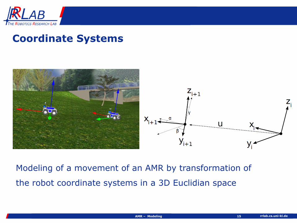
rrlabcsuni-klde
Coordinate Systems
AMR ndash Modeling 15
Modeling of a movement of an AMR by transformation of
the robot coordinate systems in a 3D Euclidian space
rrlabcsuni-kldeAMR ndash Modeling 16
Description of AMR Pose as Six-Tuple
In general the pose of an arbitrary object in the Cartesian space can be described as a six-tuple 119909 119910 119911 120593 120595 120579
The position vector 119874119906 in an object frame 119874 can be presented
in base frame coordinates 119861119906 by
119861119906 =119909119910119911
+ 119874119861119877 120593120595 120579 119874 119906
with 119909 119910 119911 119879 being the translation vector between the origin of the two frames and 119877 (3x3 matrix) the respective (combined) rotation matrix
rrlabcsuni-kldeAMR ndash Modeling 17
Homogeneous Transformation Matrix
Another possibility to express the same as above are homogeneous transformation matrices Those 4 times 4 matrices(for 3D space) are composed as shown below
119877 119906Ԧ119901119879 119904
119877 3 times 3 rotation (orientation) matrix
119906 Translation (position) - 119906 = 119906119909 119906119910 119906119911119879
Ԧ119901 Perspective transformation in general Ԧ119901 = 000 119879
119904 Scaling factor in general 119904 = 1
rrlabcsuni-kldeAMR ndash Modeling 18
3D Rotation Matrices
119877 is usually a combination of several rotations around the elementary axis
119877119909 120593 describes a rotation around the x-axis of an arbitrary coordinate system via the angle 120593 In an analog matter the other two required matrices are defined
119877119909 120593 =1 0 00 cos120593 minus sin1205930 sin120593 cos120593
119877119910 120595 =cos120595 0 sin1205950 1 0
minus sin120595 0 cos120595
119877119911 θ =cos θ minus sin θ 0sin θ cos θ 00 0 1 119909 119906
120593 119910
119907
119911119908
rrlabcsuni-kldeAMR ndash Modeling 19
Expression of Linked Rotations
Two possible ways of expressing linked rotations
Euler angles (rotation around variable axes)
119877 = 119877119911 120593 sdot 119877119909 120595 sdot 119877119911prime θ
Tait-Bryan angles ldquoRoll Pitch Yawrdquo (rotation around fixed axes)
119877 = 119877119911 θ sdot 119877119910 120595 sdot 119877119909 120593
rrlabcsuni-kldeAMR ndash Modeling 20
Roll Pitch Yaw
Euler rotations along ldquonewrdquo axes
Roll-Pitch-Yaw rotations along fixed axes
Terrestrial robotics the roll pitch yaw system is used (change of AMR pose according to world coordinate system)
Yaw θ
Pitchψ
Roll 120593
119911
119910119909
20
Roll
Pitch Yaw
119909
119911119910
rrlabcsuni-kldeAMR ndash Modeling 21
Combined Rotational Matrix (Roll Pitch Yaw)
Arbitrary orientation in 3D space can be described using three rotations
119877119904 as resulting matrix
(abbreviations 119904120593 for sin120593 and 119888120593 for cos120593)
119877119904 =
119888θ 119888120595 119888θ 119904120595 119904120593 minus 119904θ 119888120593 119888θ 119904120595 119888120593 + 119904θ 119904120593119904θ 119888120595 119904θ 119904120595 119904120593 + 119888θ 119888120593 119904θ 119904120595 119888120593 minus 119888θ 119904120593minus119904120595 119888120595 119904120593 119888120595 119888120593
rrlabcsuni-kldeAMR ndash Modeling 22
Linear Velocity
Transformation velocities between two frames is similar to pose transformation
Transformation of a linear velocity vector 119861 Ԧ119907119902 of an arbitrary
point Ԧ119902 presented in frame 119861 to frame 119860119860 Ԧ119907119902 = 119861
119860119877119861 Ԧ119907119902
If the origin of frame 119861 has also a linear velocity relative to frame 119860 then
119860 Ԧ119907119902 =119860 Ԧ119907119874119861 + 119861
119860119877119861 Ԧ119907119902
If in addition point Ԧ119902 is rotating around an arbitrary axis with
the rotational velocity 119860Ω119861 then the linear velocity can be
calculated with
119860 Ԧ119907119876 = 119860 Ԧ119907119874119861 + 119861119860119877119861 Ԧ119907119876 +
119860ω119861 times 119861119860119877119861 Ԧ119902
rrlabcsuni-kldeAMR ndash Modeling 23
Rotational Velocity
A rotational vector 119861120596 related to frame 119861 can be transferred
to frame 119860 with
119860120596 = 119861119860119877119861120596
rrlabcsuni-kldeAMR ndash Modeling 24
Linear and Rotational Velocity
Rotational and linear velocity of a sequence of segments connected by rotational or prismatic joints can stepwise be calculated
Rotational velocity 119894+1120596119894+1 and the linear velocity 119894+1 Ԧ119907119894+1relative to frame 119894 + 1 can be determined as
119894+1120596119894+1 = 119894119894+1119877 sdot 119894120596119894 + ሶθ119894+1
119894+1 Ԧ119890119911119894+1
119894+1 Ԧ119907119894+1 = 119894119894+1119877 119894 Ԧ119907119894 +
119894120596119894 times119894 Ԧ119901119894+1
with 119894 Ԧ119901119894+1 vector in direction of the segment 119894 120596119894 the rotational
velocity and 120595119894 the rotation of segment 119894 around the elementary 119911-axis
rrlabcsuni-kldeAMR ndash Modeling 25
Linear and Rotational Velocity
119894119894+1119877 is the inverse of the orientation matrix 119894+1
119894119877 from frame 119894 to
119894 + 1
119894+1119894119877 is an orthonormal matrix
its inverse 119894+1119894119877minus1 = 119894
119894+1119877 is the transposed matrix 119894+1119894119877119879
(example in 2D space)
119894119894+1119877 θ = 119894+1
119894119877minus1 θ = 119894+1119894119877119879 θ =
119888θ 119904θ 119909119908minus119904θ 119888θ 1199101199080 0 1
rrlabcsuni-klde
World (Global) and Robot (Local) Coordinate System
AMR ndash Modeling 26
YW
XW
θ
YR
XR
P
rrlabcsuni-kldeAMR ndash Modeling 27
World and Robot Coordinate System
119875 describes the location of the kinematic center relative to the world coordinate system
120579 is the mathematically positive angle between 119883119882 and 119883119877 119874 119883119882 119884119882 ෝ= origin of the world coordinate system
119874 119883119877 119884119877 ෝ= 119875 ෝ= origin of the robotrsquos coordinate system
119883119877-axis is longitudinal axis of the robot through its kinematic center
119884119877-axis is lateral axis of the robot through its kinematics center
120585119882 = 119909 119910 120579 119879 coordinates of the kineamtic center in world
coordinates
rrlabcsuni-kldeAMR ndash Modeling 28
World and Robot Coordinate System
Orientation via rotation around 119911-axis
119877 θ =cos θ sin θ 0minussin θ cos θ 0
0 0 1
Speed transformation from world- to robot coordinate system
ሶԦ120585119877 = 119877 θሶԦ120585119882
Coordinate transformation
YW
XW
θ
YR
XR
rrlabcsuni-kldeAMR ndash Modeling 29
World and Robot Coordinate System
Rotation around 119911-axis withθ = 90 deg
119877120587
2=
0 1 0minus1 0 00 0 1
Speed calculation in robot coordinates
ሶԦ120585119877 = 119877120587
2ሶ
120585119882 =0 1 0minus1 0 00 0 1
sdotሶ119909ሶ119910ሶθ
=ሶ119910
minus ሶ119909ሶθ
rrlabcsuni-klde
Vehicle Kinematics -
Analytical Solution
rrlabcsuni-kldeAMR ndash Kinematics 31
Control of the Test Vehicle GATOR
rrlabcsuni-kldeAMR ndash Kinematics 32
Forward kinematics for wheel driven robot
What is the robotrsquos trajectory if wheel geometry and speed are known
YW
XW
θ
V(t)
120596(t)
rrlabcsuni-kldeAMR ndash kinematics 33
Example Differential Drive
119903 radius of the wheel
119889 distance wheel center to kinematic center
ሶ120595119903 ሶ120595119897 Angular velocity of leftright wheel
ሶԦ120585119882 speed calculation in world coordinates
ሶԦ120585119882 = ሶ119909 ሶ119910 ሶ120579119879
= 119891 119889 119903 120579 ሶ120595119897 ሶ120595119903
= 119877 120579 minus1 ሶԦ120585119877
passive wheel
active wheel
d
rrlabcsuni-kldeAMR ndash Kinematics 34
Example Differential Drive
Calculation of the contribution of the left and right wheel to the speed along the longitudinal axis (119883119877)
Calculation of the contribution of the left and right wheel to the angular velocity of kinematic center
Summation of both results in the velocity and angular velocity along the 119883119877-axis where
ሶ119909119877119903 =119903 ሶ1205951199032
ሶ119909119877119897 =119903 ሶ120595119897
2
120596119903 =119903 ሶ1205951199032119889
120596119897 =minus119903 ሶ120595119897
2119889
ሶԦ120585119882 = 119877 120579 minus1 ሶԦ120585119903ሶԦ120585119903 =
119903 ሶ1205951199032
+119903 ሶ120595119897
2 0
119903 ሶ1205951199032119889
minus119903 ሶ120595119897
2119889
119879
rrlabcsuni-kldeAMR ndash Kinematics 35
Example Differential Drive
Since 119877 120579 is orthonormal
119877 120579 minus1 =cos 120579 minus sin 120579 0sin 120579 cos 120579 00 0 1
Given 120579 =120587
2 119903 = 1 119889 = 1 ሶ120595119903 = 4 ሶ120595119897 = 2 and wheel speed
notated in rounds per second 2120587
119904
ሶԦ120585119882 =ሶ119909ሶ119910ሶ120579
=0 minus1 01 0 00 0 1
sdot301
=031
rrlabcsuni-kldeAMR ndash Kinematics 36
Calculation of Wheel kinematics
Stepwise calculation of the linear and the rotational velocity for wheeled vehicles in 2D environment
Kinematic center moved with ሶ119909 ሶ119910 ሶ120579119879
Determine rotational velocity of each wheel
Collect all equations and solve the equation system
Consider
Equation system must no be solvable
No dynamic aspects will be considered
Calculation of the speed of the kinematic center based on thewheel speed can also be determined out of the equationsystem (inverse problem)
rrlabcsuni-klde
Basic Wheel Types
AMR ndash Kinematics 37
Standardwheel
Steerablestandard
wheel
Castorwheel
Swedish orMecanum
wheel
Ball orspherical
wheel
rrlabcsuni-kldeAMR ndash Kinematics 38
Wheel Properties
Standard and steerable wheel
Linear velocity along wheel plane ሶ119909 = 119903 ሶ120595
No sliding orthogonal to wheel plane ሶ119910 = 0
Castor wheel
Linear velocity along wheel plane ሶ119909 = 119903 ሶ120595
Linear perpendicular velocity ሶ119910 = minus119889119888 ሶ120573
SwedishMecanum wheel
Linear velocity along wheel plane ሶ119909 = 119903 ሶ120595 cos 120574
120574 angle of passive rollers (45 deg or 90 deg)
Linear perpendicular velocity ሶ119910 = 119903 ሶ120595 sin 120574 + 119903119901119903 ሶ120595119901119903
rrlabcsuni-kldeAMR ndash Kinematics 39
Kinematic Parameters
rrlabcsuni-kldeAMR ndash Kinematics 40
Kinematic Parameters
120572 Angle between 119909-axis and wheel mount point
120573 Angle between the straight line through the kinematic center and the fixing point of the wheel and the 119910-axis of the wheel frame
119889 Distance from the kinematic center to the wheel fixingpoint
119889119888 Distance from the wheel fixing point to the wheel supporting point (Castor wheel only)
120574 Angle between the 119909-axis of the wheel and rolling direction of the rollers (Mecanum wheel only)
rrlabcsuni-kldeAMR ndash Kinematics 41
Kinematic Parameters Standard Wheel
ሶ120595 119903
rrlabcsuni-kldeAMR ndash Kinematics 42
Kinematic Parameters Steerable Wheel
ሶ120595 119903
rrlabcsuni-kldeAMR ndash Kinematics 43
Kinematic Parameters Castor Wheel
ሶ120595 119903
rrlabcsuni-kldeAMR ndash Kinematics 44
Kinematic Parameters Mecanum Wheel
ሶ120595 119903
rrlabcsuni-kldeAMR ndash Kinematics 45
Kinematic Parameters Ball Wheel
ሶ120595 119903
rrlabcsuni-kldeAMR ndash Kinematics 46
Calculation of Wheel Velocity
Given velocity vector Ԧ119907 = ሶ119909 ሶ119910 ሶ120579119879
of the kinematic center
Calculation of linear velocity of standard wheel due to the speed of the kinematic center
Stepwise apply the following equations
Initial parameters 11205961 = 00 ሶ120579119879
and 1 Ԧ1199071 = ሶ119909 ሶ119910 0 119879
No additional rotational speed all 119894120596119894 = 00 ሶ120579119879
119894+1120596119894+1 = 119894119894+1119877 sdot 119894120596119894 + ሶ120579119894+1
119894+1 Ԧ119890119911119894+1
119894+1 Ԧ119907119894+1 = 119894119894+1119877 119894 Ԧ119907119894 +
119894120596119894 times119894 Ԧ119901119894+1
rrlabcsuni-kldeAMR ndash Kinematics 47
Calculation of Wheel Velocity
After the rotation around the 119911-axis with angle 120572 2 Ԧ1199072 is
calculated as
2 Ԧ1199072 =119888120572 ሶ119909 + 119904120572 ሶ119910minus119904120572 ሶ119909 + 119888120572 ሶ119910
0
Due to the translation 119889 3 Ԧ1199073 is
3 Ԧ1199073 =
119888120572 ሶ119909 + 119904120572 ሶ119910
minus119904120572 ሶ119909 + 119888120572 ሶ119910 + 119889 ሶ1205790
rrlabcsuni-kldeAMR ndash Kinematics 48
Calculation of Wheel Velocity
The last rotation around the 119911-axis with angle 120573 minus 90degtransfers the 119909-axis of the last frame to the rolling direction of the wheel
For the calculation of 4 Ԧ1199074 in the next equation
sin 120573 minus 90deg = minus cos120573 and cos 120573 minus 90deg = sin 120573 is used
4 Ԧ1199074 =119904 120572 + 120573 ሶ119909 minus 119888 120572 + 120573 ሶ119910 minus 119888120573 119889 ሶ120579
119888 120572 + 120573 ሶ119909 + 119904 120572 + 120573 ሶ119910 + 119904120573 119889 ሶ1205790
rrlabcsuni-kldeAMR ndash 4 Modeling 49
Calculation of Wheel Velocity
Last step is to equalize the linear velocity vector of the standard wheel to the velocity of the kinematic center represented in the wheel frame
119904 120572 + 120573 minus119888 120572 + 120573 minus119888120573 119889
119888 120572 + 120573 119904 120572 + 120573 119904120573 1198890 0 0
ሶ119909119910 ሶሶ120579
=119903 ሶ12059500
1st equation 119903 ሶ120595 = 119888 120572 + 120573 ሶ119909 + 119904 120572 + 120573 ሶ119910 + 119904120573 119889 ሶ120579 is called the
rolling constraint of the wheel because it describes the speed in the rolling direction of the wheel
2nd equation 119888 120572 + 120573 ሶ119909 + 119904 120572 + 120573 ሶ119910 + 119904120573 119889 ሶ120579 = 0 is called the
sliding constraint which describes the speed perpendicular to wheel plane
Sliding constraints are collected in Matrix 119878 ndash add row (119888(120572 +
rrlabcsuni-kldeAMR ndash Kinematics 50
Wheel Type-specific Velocity Vector
In case of the steerable standard wheel the fixed angle 120573 is replaced by a function 120573 119905
Equation could also be applied to the spherical wheel (based on the forces which affect the wheel and change 120573 119905 only a linear velocity in the rolling direction exists)
In case of castor wheels the y-component of the velocity
vector is depending on the angular velocity ሶ120573 and the length of the rod
119904 120572 + 120573(119905) minus119888 120572 + 120573(119905) minus119888120573(119905)119889
119888 120572 + 120573(119905) 119904 120572 + 120573(119905) 119904120573(119905)1198890 0 0
ሶ119909ሶ119910ሶ120579
=119903 ሶ120595
minus119889119888 ሶ120573(119905)0
Sliding constraints are collected in Matrix 119878 ndash add row 119888 120572 + 120573(119905) 119904 120572 + 120573(119905) 119904120573(119905)119889 (is used in section
maneuverability)
rrlabcsuni-kldeAMR ndash 4 Modeling 51
Wheel Type-specific Velocity Vector
Swedish or Mecanum wheel is able to move in an omnidirectional way
119904 120572 + 120573 + 120574 minus119888 120572 + 120573 + 120574 minus119888 120573 + 120574 119889
119888 120572 + 120573 + 120574 119904 120572 + 120573 + 120574 119904 120573 + 120574 1198890 0 0
ሶ119909ሶ119910ሶ120579
=119903 ሶ120595 cos 120574
119903 ሶ120595 sin 120574 + 119903119901119903 ሶ1205951199011199030
rrlabcsuni-kldeAMR ndash Kinematics 52
Vehicle Motion Calculation
Transformation of wheel velocities to velocity of kinematic center
Determine parameters 120572 120573 120574d indicating the wheel pose
Insert 120572 120573 120574 into appropriate wheel equation (as shown before) for each wheel
Solve system of equations
rrlabcsuni-kldeAMR ndash Kinematics 53
Differential Drive Kinematics
Two fixed standard wheels mounted on one axis
Kinematic center located in the middle of the axis
Distance between the kinematic center and each wheel 119889
Kinematic center is origin of coordinate frame
One solution for modeling the wheel configuration is to place the wheels on the 119910-axis
Kinematic parameters
120572119897 = 90 deg
120573119897 = 0 deg
120572119903 = minus90 deg
120573119903 = 180 deg
rrlabcsuni-kldeAMR ndash Kinematics 54
Differential Drive Kinematics
Apply equations for standard wheels (for the left and the right wheel)
119904 120572119897 + 120573119897 ሶ119909 minus 119888 120572119897 + 120573119897 ሶ119910 minus 119888120573119897 119889 ሶ120579 = 119903119897 ሶ120595119897
119888 120572119897 + 120573119897 ሶ119909 + 119904 120572119897 + 120573119897 ሶ119910 + 119904120573119897 119889 ሶ120579 = 0
119904 120572119903 + 120573119903 ሶ119909 minus 119888 120572119903 + 120573119903 ሶ119910 minus 119888120573119903 119889 ሶ120579 = 119903119903 ሶ120595119903119888 120572119903 + 120572119903 ሶ119909 + 119904 120572119903 + 120573119903 ሶ119910 + 119904120573119903 119889 ሶ120579 = 0
If the above mentioned parameters are inserted the following equations will result
ሶ119909 minus 119889 ሶ120579 = 119903119897 ሶ120595119897
ሶ119910 = 0
ሶ119909 + 119889 ሶ120579 = 119903119903 ሶ120595119903119910 = 0
rrlabcsuni-kldeAMR ndash Kinematics 55
Differential Drive Kinematics
Solving the system of equations yields
ሶ119909ሶ119910ሶ120579
=
1
2119903119897 ሶ120595119897 + 119903119903 ሶ120595119903
01
2119889minus119903119897 ሶ120595119897 + 119903119903 ሶ120595119903
rrlabcsuni-kldeAMR ndash Kinematics 56
Differential Drive Kinematics of MARVIN
rrlabcsuni-klde
CROMSCI ndash Equipped with 3 Steerable Standard Wheels
AMR ndash Kinematics 57
Climbing robot CROMSCI Wheel settings of CROMSCI
rrlabcsuni-klde
Omnidirectional Drive Kinematics
AMR ndash Kinematics 58
Typical orientations of the 3 steerable wheels of an omnidirectional vehicle
rrlabcsuni-kldeAMR ndash Kinematicsg 59
Omnidirectional Drive Kinematics
Three steerable standard wheels
Kinematic center located in the middle of the robot
Distance between the kinematic center and each wheel 119889
Origin of coordinates frame is kinematic center
Kinematic parameters
1205721 = 0 deg
1205722 = 120 deg
1205723 = minus120 deg
rrlabcsuni-kldeAMR ndash Kinematics 60
Omnidirectional Drive Kinematics
Applying equation for steerable standard wheel for each wheel leads to the following system of equations
119904 1205721 + 1205731 ሶ119909 minus 119888 1205721 + 1205731 ሶ119910 minus 119889 sdot 119888 1205731 ሶ120579 = 1199031 ሶ1205951
119904 1205722 + 1205732 ሶ119909 minus 119888 1205722 + 1205732 ሶ119910 minus 119889 sdot 119888 1205732 ሶ120579 = 1199032 ሶ1205952
119904 1205723 + 1205733 ሶ119909 minus 119888 1205723 + 1205733 ሶ119910 minus 119889 sdot 119888 1205733 ሶ120579 = 1199033 ሶ1205953
119888 1205721 + 1205731 ሶ119909 + 119904 1205721 + 1205731 ሶ119910 + 119889 sdot 119904 1205731 ሶ120579 = 0
119888 1205722 + 1205732 ሶ119909 + 119904 1205722 + 1205732 ሶ119910 + 119889 sdot 119904 1205732 ሶ120579 = 0
119888 1205723 + 1205733 ሶ119909 + 119904 1205723 + 1205733 ሶ119910 + 119889 sdot 119904 1205733 ሶ120579 = 0
rrlabcsuni-kldeAMR ndash Kinematics 61
Omnidirectional Drive Kinematics
Based on these equation the steering angles 120573119894 119894 = 123 can be determined
119888 120572119894 + 120573119894 sdot ሶ119909 + 119904 120572119894 + 120573119894 sdot ሶ119910 + 119889 sdot 119904 120573119894 sdot ሶ120579 = 0
119888 120572119894 sdot 119888 120573119894 sdot ሶ119909 minus 119904 120572119894 sdot 119904 120573119894 sdot ሶ119909 + 119904 120572119894 sdot 119888 120573119894 sdot ሶ119910 + 119888 120572119894 sdot 119904 120573119894 sdot ሶ119910 + 119889 sdot 119904 120573119894 sdot ሶ120579 = 0
119888 120573119894 sdot 119888 120572119894 sdot ሶ119909 + 119904 120572119894 sdot ሶ119910 minus 119904 120573119894 sdot 119904 120572119894 sdot ሶ119909 minus 119888 120572119894 sdot ሶ119910 minus 119889 sdot ሶ120579 = 0
119888 120572119894 sdot ሶ119909 + 119904 120572119894 sdot ሶ119910
119904 120572119894 sdot ሶ119909 minus 119888 120572119894 sdot ሶ119910 minus 119889 sdot ሶ120579=119904 120573119894119888 120573119894
atan2 119888 120572119894 sdot ሶ119909 + 119904 120572119894 sdot ሶ119910 119904 120572119894 sdot ሶ119909 minus 119888 120572119894 sdot ሶ119910 minus 119889 sdot ሶ120579 = 120573119894
Also the angular velocity of the wheel ሶ120595119894 can now be calculated
ሶ120595119894 =1
119903119894119904 120572119894 + 120573119894 ሶ119909 minus 119888 120572119894 + 120573119894 ሶ119910 minus 119889 sdot 119888 120573119894 ሶ120579
rrlabcsuni-klde
The Climbing Robot CROMSCI
AMR ndash Kinematics 62
rrlabcsuni-klde
Mecanum Vehicle
AMR ndash Kinematics 63
Schematic configurationof a Mecanum wheel(Viewed from above)
The mobile robot PRIAMOS of the University of Karlsruhe driven by Mecanum wheels
rrlabcsuni-kldeAMR ndash Kinematics 64
Mecanum Kinematics
To set up the kinematic equation first the parameters 120572 120573 120574for each wheel must be determined
The parameters for four wheels are
1205721 = 45 deg 1205731 = 45 deg 1205741 = minus45 deg
1205722 = 135 deg 1205732 = minus45 deg 1205742 = 45 deg
1205723 = minus135 deg 1205733 = 225 deg 1205743 = minus45 deg
1205724 = minus45 deg 1205734 = 135 deg 1205744 = 45 deg
rrlabcsuni-kldeAMR ndash Kinematics 65
Mecanum Kinematics
Assume all driven wheels have the same radius 119903 the same distance 119889 from the kinematic center and the above mentioned parameters 120572 120573 120574
Using equation for Mecanum wheels leads to equations
119904 45 deg ሶ119909 minus 119888 45 deg ሶ119910 minus 119889 ሶ120579 = 119903 sdot 119888 minus45 deg ሶ1205951
119904 135 deg ሶ119909 minus 119888 135 deg ሶ119910 minus 119889 ሶ120579 = 119903 sdot 119888 45 deg ሶ1205952
119904 45 deg ሶ119909 minus 119888 45 deg ሶ119910 minus 119889 ሶ120579 = 119903 sdot 119888 minus45 deg ሶ1205953
119904 135 deg ሶ119909 minus 119888 135 deg ሶ119910 minus 119889 ሶ120579 = 119903 sdot 119888 45 deg ሶ1205954
rrlabcsuni-kldeAMR ndash Kinematics 66
Mecanum Kinematics
The velocities ሶ119909 ሶ119910 ሶ120579 of the kinematic center can be calculated
ሶ119909 =119903
4ሶ1205951 + ሶ1205952 + ሶ1205953 + ሶ1205954
ሶ119910 =119903
4minus ሶ1205951 + ሶ1205952 minus ሶ1205953 + ሶ1205954
ሶ120579 =119903
119889 2ሶ1205951 minus ሶ1205952 minus ሶ1205953 + ሶ1205954
rrlabcsuni-kldeAMR ndash Kinematics 67
Mecanum Kinematics
The velocity vector of the kinematic center can be determined as
ሶ119909ሶ119910ሶ120579
=119903119908ℎ1198901198901198974
sdot1 1 1 1minus1 1 minus1 1119886 minus119886 minus119886 119886
sdot
ሶ1205951
ሶ1205952
ሶ1205953
ሶ1205954
with a =2 2
119889
Assuming the absence of slip the following must hold
ሶ1205954 = ሶ1205951 + ሶ1205952 minus ሶ1205953
rrlabcsuni-klde
Maneuverability of AMRs
rrlabcsuni-kldeAMR ndash Maneuverability 69
Choice of Wheel Configuration
Choice of wheels and their configuration depends on hellip
Ability to maneuver
Controllability
Stability
An optimum can only be achieved concerning a specific application
rrlabcsuni-kldeAMR ndash Maneuverability 70
Stability
Minimal number of wheels for static stability is 2 if center of gravity is located under the wheel axis (e g robot Cye)
Under standard conditions itrsquos 3
If more than 3 wheels are present adjustment to rough terrain becomes necessary
Typical setups
2 driven wheels on a single axis with 1 or 2 passive castor wheels
Single driven and steered wheel with two passive fixed wheels
rrlabcsuni-kldeAMR ndash Maneuverability 71
Maneuverability
Robotrsquos degree of freedom (DOF)
Outstanding ability to maneuver when the only driven wheel can be rotated in an active way
Example Ackermann steering
Poor ability to maneuver
5 m radius required for single rotation of a car
Lateral movement only possible troughforwardbackward movement
rrlabcsuni-kldeAMR ndash Maneuverability 72
Controllability
Costs for locomotion of the robot on a given trajectory
Contradiction to the robotrsquos ability to maneuver
Examples
Ackermann steering easy to control
Mecanum wheels very costly if high precision is required
Costs for controllability depend on hellip
Wheel type
Drive geometry
Sensors to determine driving situation
Motortransmission
rrlabcsuni-kldeAMR ndash Maneuverability 73
Degree of Mobility
The degree of mobility 119891119898 isin 123 points out how the sliding constraints (defined in Matrix 119878 see slide 42) affect the
possibilities for robot movement 119877 120579 ሶ120585119897 The mobility can be calculated by using the rank of the
matrix of sliding constraints of all standard wheels (steerable and fixed wheels) = number of independent constraints
119891119898 = 3 minus rank 119878
rrlabcsuni-kldeAMR ndash Maneuverability 74
Degree of Mobility
Example Differential Drive
Given only two fixed wheels geometrically we can set
1198891 = 1198892 1205731 = 1205732 = 0 1205721 + 120587 = 1205722
Matrix 119878 has two sliding constraints of the form (119888(120572 +
rrlabcsuni-kldeAMR ndash Maneuverability 75
Degree of Steerability
The degree of steerability 119891119904 isin 012 quantifies the degree of controllable freedom and is determined via the number of independently controllable steering parameters
Define 119878prime Part of 119878 defining sliding constraints of steerable wheels
119891119904 = rank 119878prime
More possibilities in steering will result in lower mobility
119891119904 = 0 No steered wheel (differential drive)
119891119904 = 1 At least one steered wheel (Ackermann steering)
119891119904 = 2 At least two steered wheels no fixed wheel
rrlabcsuni-kldeAMR ndash Maneuverability 76
Degree of Maneuverability
The degree of maneuverability 119891119872 isin 23 points out the number of DOF the robot can manipulate
119891119872 = 119891119898 + 119891119904
rrlabcsuni-klde
Vehicle Kinematics
Geometrical Solution
rrlabcsuni-kldeAMR ndash Kinematics 78
Tricycle Drive
Given 120575 119907
Unknown 119907prime 119907119897 119907119903 Solution
119903 = 119897 sdot cot 120575
119907prime =119907
cos 120575
119907119897 = 119907 sdot119903 + 119889
119903
119907119903 = 119907 sdot119903 minus 119889
119903 Tricycle drive kinematics
120575
rrlabcsuni-kldeAMR ndash 4 Kinematics 79
Ackermann Steering
Given 119907119863 120575 119897 119889
Unknown 119907119903119903 119907119897119903 119907119903119891 119907119897119891
Solution
120602 =119897
tan 120575
119907119897119903 =120602 minus 1198892 sdot 119907119863
120602
119907119903119903 =120602 + 1198892 sdot 119907119863
120602
119907119897119891 =120602 minus 1198892 2 + 1198972 sdot tan 120575
119897sdot 119907119863
119907119903119891 =1206022 + 1198972 sdot tan 120575
119897sdot 119907119863
Kinematics ofAckermann steering
120575
120602
rrlabcsuni-klde
Omnidrive Kinematics
AMR ndash Kinematics 80
Given 120602 120593 119907 119889
Unknown 1205931 1205932 1199071 1199072 Solution
120549119909 = 120602 sdot cos120593120549119910 = 120602 sdot sin1205931205931 = arctan120549119910 minus 1198891205491199091206021 = 120602 sdot cos120593 cos12059311199071 = 119907 sdot 1206021120602
1205932 = arctan120549119910 + 119889
1205491199091206022 = 120602 sdot cos120593 cos1205932
1199072 = 119907 sdot 1206022120602
120549119910 = 120602 ∙ 119904119894119899 120593
1205931
1205932
1206021
1206022
120593 120549119909 = 120602 ∙ cos120593
120602
119889
rrlabcsuni-klde
Bicycle Model
AMR ndash Kinematics 81
119907
rrlabcsuni-kldeAMR ndash Kinematics 82
Bicycle Model
Circular road of radius 120602
Low speed motion
Slip angles at both wheels are zero
Small total lateral force from both tires
119865119910 =1198981199072
120602
Point 119875 is instantaneous rolling center
Velocity at 119862 is perpendicular to line 119875119862
Heading angle 120579
Slip angle 120575119907 Course angle 120574 = 120579 + 120575119907
rrlabcsuni-kldeAMR ndash 4 Modeling 83
Bicycle Model
Given 120575119891 120575119903 119907 120579
Unknown ሶ119883 ሶ119884 ሶ120579
Solution
120575119907 = tanminus1119897119891 tan 120575119903+119897119903 tan 120575119891
119897119891+119897119903
ሶ120579 =119907
120602
120602 =119897119891+119897119903
tan 120575119891 minustan 120575119903 cos 120575119907
ሶ119883 = 119907 cos 120579 + 120575119907ሶ119884 = 119907 sin 120579 + 120575119907
ሶ120579 =119907 cos 120575119907
119897119891+119897119903tan 120575119891 minus tan 120575119903
119907
rrlabcsuni-klde
Ackermann Steering -gt Bicycle Model
AMR ndash Kinematics 84
119862 = 119874 120575119903 = 0 120575119891 = 120575
119897119903 = 0 119897119891 = 119897
120575119907 = 0
ሶ120579 =119907
120602
120602 =119897
tan 120575119891
ሶ119883 = 119907 cos 120579ሶ119884 = 119907 sin 120579ሶ120579 =
119907
119897119891tan 120575119891
119907

rrlabcsuni-klde
World (Global) and Robot (Local) Coordinate System
AMR ndash Modeling 26
YW
XW
θ
YR
XR
P
rrlabcsuni-kldeAMR ndash Modeling 27
World and Robot Coordinate System
119875 describes the location of the kinematic center relative to the world coordinate system
120579 is the mathematically positive angle between 119883119882 and 119883119877 119874 119883119882 119884119882 ෝ= origin of the world coordinate system
119874 119883119877 119884119877 ෝ= 119875 ෝ= origin of the robotrsquos coordinate system
119883119877-axis is longitudinal axis of the robot through its kinematic center
119884119877-axis is lateral axis of the robot through its kinematics center
120585119882 = 119909 119910 120579 119879 coordinates of the kineamtic center in world
coordinates
rrlabcsuni-kldeAMR ndash Modeling 28
World and Robot Coordinate System
Orientation via rotation around 119911-axis
119877 θ =cos θ sin θ 0minussin θ cos θ 0
0 0 1
Speed transformation from world- to robot coordinate system
ሶԦ120585119877 = 119877 θሶԦ120585119882
Coordinate transformation
YW
XW
θ
YR
XR
rrlabcsuni-kldeAMR ndash Modeling 29
World and Robot Coordinate System
Rotation around 119911-axis withθ = 90 deg
119877120587
2=
0 1 0minus1 0 00 0 1
Speed calculation in robot coordinates
ሶԦ120585119877 = 119877120587
2ሶ
120585119882 =0 1 0minus1 0 00 0 1
sdotሶ119909ሶ119910ሶθ
=ሶ119910
minus ሶ119909ሶθ
rrlabcsuni-klde
Vehicle Kinematics -
Analytical Solution
rrlabcsuni-kldeAMR ndash Kinematics 31
Control of the Test Vehicle GATOR
rrlabcsuni-kldeAMR ndash Kinematics 32
Forward kinematics for wheel driven robot
What is the robotrsquos trajectory if wheel geometry and speed are known
YW
XW
θ
V(t)
120596(t)
rrlabcsuni-kldeAMR ndash kinematics 33
Example Differential Drive
119903 radius of the wheel
119889 distance wheel center to kinematic center
ሶ120595119903 ሶ120595119897 Angular velocity of leftright wheel
ሶԦ120585119882 speed calculation in world coordinates
ሶԦ120585119882 = ሶ119909 ሶ119910 ሶ120579119879
= 119891 119889 119903 120579 ሶ120595119897 ሶ120595119903
= 119877 120579 minus1 ሶԦ120585119877
passive wheel
active wheel
d
rrlabcsuni-kldeAMR ndash Kinematics 34
Example Differential Drive
Calculation of the contribution of the left and right wheel to the speed along the longitudinal axis (119883119877)
Calculation of the contribution of the left and right wheel to the angular velocity of kinematic center
Summation of both results in the velocity and angular velocity along the 119883119877-axis where
ሶ119909119877119903 =119903 ሶ1205951199032
ሶ119909119877119897 =119903 ሶ120595119897
2
120596119903 =119903 ሶ1205951199032119889
120596119897 =minus119903 ሶ120595119897
2119889
ሶԦ120585119882 = 119877 120579 minus1 ሶԦ120585119903ሶԦ120585119903 =
119903 ሶ1205951199032
+119903 ሶ120595119897
2 0
119903 ሶ1205951199032119889
minus119903 ሶ120595119897
2119889
119879
rrlabcsuni-kldeAMR ndash Kinematics 35
Example Differential Drive
Since 119877 120579 is orthonormal
119877 120579 minus1 =cos 120579 minus sin 120579 0sin 120579 cos 120579 00 0 1
Given 120579 =120587
2 119903 = 1 119889 = 1 ሶ120595119903 = 4 ሶ120595119897 = 2 and wheel speed
notated in rounds per second 2120587
119904
ሶԦ120585119882 =ሶ119909ሶ119910ሶ120579
=0 minus1 01 0 00 0 1
sdot301
=031
rrlabcsuni-kldeAMR ndash Kinematics 36
Calculation of Wheel kinematics
Stepwise calculation of the linear and the rotational velocity for wheeled vehicles in 2D environment
Kinematic center moved with ሶ119909 ሶ119910 ሶ120579119879
Determine rotational velocity of each wheel
Collect all equations and solve the equation system
Consider
Equation system must no be solvable
No dynamic aspects will be considered
Calculation of the speed of the kinematic center based on thewheel speed can also be determined out of the equationsystem (inverse problem)
rrlabcsuni-klde
Basic Wheel Types
AMR ndash Kinematics 37
Standardwheel
Steerablestandard
wheel
Castorwheel
Swedish orMecanum
wheel
Ball orspherical
wheel
rrlabcsuni-kldeAMR ndash Kinematics 38
Wheel Properties
Standard and steerable wheel
Linear velocity along wheel plane ሶ119909 = 119903 ሶ120595
No sliding orthogonal to wheel plane ሶ119910 = 0
Castor wheel
Linear velocity along wheel plane ሶ119909 = 119903 ሶ120595
Linear perpendicular velocity ሶ119910 = minus119889119888 ሶ120573
SwedishMecanum wheel
Linear velocity along wheel plane ሶ119909 = 119903 ሶ120595 cos 120574
120574 angle of passive rollers (45 deg or 90 deg)
Linear perpendicular velocity ሶ119910 = 119903 ሶ120595 sin 120574 + 119903119901119903 ሶ120595119901119903
rrlabcsuni-kldeAMR ndash Kinematics 39
Kinematic Parameters
rrlabcsuni-kldeAMR ndash Kinematics 40
Kinematic Parameters
120572 Angle between 119909-axis and wheel mount point
120573 Angle between the straight line through the kinematic center and the fixing point of the wheel and the 119910-axis of the wheel frame
119889 Distance from the kinematic center to the wheel fixingpoint
119889119888 Distance from the wheel fixing point to the wheel supporting point (Castor wheel only)
120574 Angle between the 119909-axis of the wheel and rolling direction of the rollers (Mecanum wheel only)
rrlabcsuni-kldeAMR ndash Kinematics 41
Kinematic Parameters Standard Wheel
ሶ120595 119903
rrlabcsuni-kldeAMR ndash Kinematics 42
Kinematic Parameters Steerable Wheel
ሶ120595 119903
rrlabcsuni-kldeAMR ndash Kinematics 43
Kinematic Parameters Castor Wheel
ሶ120595 119903
rrlabcsuni-kldeAMR ndash Kinematics 44
Kinematic Parameters Mecanum Wheel
ሶ120595 119903
rrlabcsuni-kldeAMR ndash Kinematics 45
Kinematic Parameters Ball Wheel
ሶ120595 119903
rrlabcsuni-kldeAMR ndash Kinematics 46
Calculation of Wheel Velocity
Given velocity vector Ԧ119907 = ሶ119909 ሶ119910 ሶ120579119879
of the kinematic center
Calculation of linear velocity of standard wheel due to the speed of the kinematic center
Stepwise apply the following equations
Initial parameters 11205961 = 00 ሶ120579119879
and 1 Ԧ1199071 = ሶ119909 ሶ119910 0 119879
No additional rotational speed all 119894120596119894 = 00 ሶ120579119879
119894+1120596119894+1 = 119894119894+1119877 sdot 119894120596119894 + ሶ120579119894+1
119894+1 Ԧ119890119911119894+1
119894+1 Ԧ119907119894+1 = 119894119894+1119877 119894 Ԧ119907119894 +
119894120596119894 times119894 Ԧ119901119894+1
rrlabcsuni-kldeAMR ndash Kinematics 47
Calculation of Wheel Velocity
After the rotation around the 119911-axis with angle 120572 2 Ԧ1199072 is
calculated as
2 Ԧ1199072 =119888120572 ሶ119909 + 119904120572 ሶ119910minus119904120572 ሶ119909 + 119888120572 ሶ119910
0
Due to the translation 119889 3 Ԧ1199073 is
3 Ԧ1199073 =
119888120572 ሶ119909 + 119904120572 ሶ119910
minus119904120572 ሶ119909 + 119888120572 ሶ119910 + 119889 ሶ1205790
rrlabcsuni-kldeAMR ndash Kinematics 48
Calculation of Wheel Velocity
The last rotation around the 119911-axis with angle 120573 minus 90degtransfers the 119909-axis of the last frame to the rolling direction of the wheel
For the calculation of 4 Ԧ1199074 in the next equation
sin 120573 minus 90deg = minus cos120573 and cos 120573 minus 90deg = sin 120573 is used
4 Ԧ1199074 =119904 120572 + 120573 ሶ119909 minus 119888 120572 + 120573 ሶ119910 minus 119888120573 119889 ሶ120579
119888 120572 + 120573 ሶ119909 + 119904 120572 + 120573 ሶ119910 + 119904120573 119889 ሶ1205790
rrlabcsuni-kldeAMR ndash 4 Modeling 49
Calculation of Wheel Velocity
Last step is to equalize the linear velocity vector of the standard wheel to the velocity of the kinematic center represented in the wheel frame
119904 120572 + 120573 minus119888 120572 + 120573 minus119888120573 119889
119888 120572 + 120573 119904 120572 + 120573 119904120573 1198890 0 0
ሶ119909119910 ሶሶ120579
=119903 ሶ12059500
1st equation 119903 ሶ120595 = 119888 120572 + 120573 ሶ119909 + 119904 120572 + 120573 ሶ119910 + 119904120573 119889 ሶ120579 is called the
rolling constraint of the wheel because it describes the speed in the rolling direction of the wheel
2nd equation 119888 120572 + 120573 ሶ119909 + 119904 120572 + 120573 ሶ119910 + 119904120573 119889 ሶ120579 = 0 is called the
sliding constraint which describes the speed perpendicular to wheel plane
Sliding constraints are collected in Matrix 119878 ndash add row (119888(120572 +
rrlabcsuni-kldeAMR ndash Kinematics 50
Wheel Type-specific Velocity Vector
In case of the steerable standard wheel the fixed angle 120573 is replaced by a function 120573 119905
Equation could also be applied to the spherical wheel (based on the forces which affect the wheel and change 120573 119905 only a linear velocity in the rolling direction exists)
In case of castor wheels the y-component of the velocity
vector is depending on the angular velocity ሶ120573 and the length of the rod
119904 120572 + 120573(119905) minus119888 120572 + 120573(119905) minus119888120573(119905)119889
119888 120572 + 120573(119905) 119904 120572 + 120573(119905) 119904120573(119905)1198890 0 0
ሶ119909ሶ119910ሶ120579
=119903 ሶ120595
minus119889119888 ሶ120573(119905)0
Sliding constraints are collected in Matrix 119878 ndash add row 119888 120572 + 120573(119905) 119904 120572 + 120573(119905) 119904120573(119905)119889 (is used in section
maneuverability)
rrlabcsuni-kldeAMR ndash 4 Modeling 51
Wheel Type-specific Velocity Vector
Swedish or Mecanum wheel is able to move in an omnidirectional way
119904 120572 + 120573 + 120574 minus119888 120572 + 120573 + 120574 minus119888 120573 + 120574 119889
119888 120572 + 120573 + 120574 119904 120572 + 120573 + 120574 119904 120573 + 120574 1198890 0 0
ሶ119909ሶ119910ሶ120579
=119903 ሶ120595 cos 120574
119903 ሶ120595 sin 120574 + 119903119901119903 ሶ1205951199011199030
rrlabcsuni-kldeAMR ndash Kinematics 52
Vehicle Motion Calculation
Transformation of wheel velocities to velocity of kinematic center
Determine parameters 120572 120573 120574d indicating the wheel pose
Insert 120572 120573 120574 into appropriate wheel equation (as shown before) for each wheel
Solve system of equations
rrlabcsuni-kldeAMR ndash Kinematics 53
Differential Drive Kinematics
Two fixed standard wheels mounted on one axis
Kinematic center located in the middle of the axis
Distance between the kinematic center and each wheel 119889
Kinematic center is origin of coordinate frame
One solution for modeling the wheel configuration is to place the wheels on the 119910-axis
Kinematic parameters
120572119897 = 90 deg
120573119897 = 0 deg
120572119903 = minus90 deg
120573119903 = 180 deg
rrlabcsuni-kldeAMR ndash Kinematics 54
Differential Drive Kinematics
Apply equations for standard wheels (for the left and the right wheel)
119904 120572119897 + 120573119897 ሶ119909 minus 119888 120572119897 + 120573119897 ሶ119910 minus 119888120573119897 119889 ሶ120579 = 119903119897 ሶ120595119897
119888 120572119897 + 120573119897 ሶ119909 + 119904 120572119897 + 120573119897 ሶ119910 + 119904120573119897 119889 ሶ120579 = 0
119904 120572119903 + 120573119903 ሶ119909 minus 119888 120572119903 + 120573119903 ሶ119910 minus 119888120573119903 119889 ሶ120579 = 119903119903 ሶ120595119903119888 120572119903 + 120572119903 ሶ119909 + 119904 120572119903 + 120573119903 ሶ119910 + 119904120573119903 119889 ሶ120579 = 0
If the above mentioned parameters are inserted the following equations will result
ሶ119909 minus 119889 ሶ120579 = 119903119897 ሶ120595119897
ሶ119910 = 0
ሶ119909 + 119889 ሶ120579 = 119903119903 ሶ120595119903119910 = 0
rrlabcsuni-kldeAMR ndash Kinematics 55
Differential Drive Kinematics
Solving the system of equations yields
ሶ119909ሶ119910ሶ120579
=
1
2119903119897 ሶ120595119897 + 119903119903 ሶ120595119903
01
2119889minus119903119897 ሶ120595119897 + 119903119903 ሶ120595119903
rrlabcsuni-kldeAMR ndash Kinematics 56
Differential Drive Kinematics of MARVIN
rrlabcsuni-klde
CROMSCI ndash Equipped with 3 Steerable Standard Wheels
AMR ndash Kinematics 57
Climbing robot CROMSCI Wheel settings of CROMSCI
rrlabcsuni-klde
Omnidirectional Drive Kinematics
AMR ndash Kinematics 58
Typical orientations of the 3 steerable wheels of an omnidirectional vehicle
rrlabcsuni-kldeAMR ndash Kinematicsg 59
Omnidirectional Drive Kinematics
Three steerable standard wheels
Kinematic center located in the middle of the robot
Distance between the kinematic center and each wheel 119889
Origin of coordinates frame is kinematic center
Kinematic parameters
1205721 = 0 deg
1205722 = 120 deg
1205723 = minus120 deg
rrlabcsuni-kldeAMR ndash Kinematics 60
Omnidirectional Drive Kinematics
Applying equation for steerable standard wheel for each wheel leads to the following system of equations
119904 1205721 + 1205731 ሶ119909 minus 119888 1205721 + 1205731 ሶ119910 minus 119889 sdot 119888 1205731 ሶ120579 = 1199031 ሶ1205951
119904 1205722 + 1205732 ሶ119909 minus 119888 1205722 + 1205732 ሶ119910 minus 119889 sdot 119888 1205732 ሶ120579 = 1199032 ሶ1205952
119904 1205723 + 1205733 ሶ119909 minus 119888 1205723 + 1205733 ሶ119910 minus 119889 sdot 119888 1205733 ሶ120579 = 1199033 ሶ1205953
119888 1205721 + 1205731 ሶ119909 + 119904 1205721 + 1205731 ሶ119910 + 119889 sdot 119904 1205731 ሶ120579 = 0
119888 1205722 + 1205732 ሶ119909 + 119904 1205722 + 1205732 ሶ119910 + 119889 sdot 119904 1205732 ሶ120579 = 0
119888 1205723 + 1205733 ሶ119909 + 119904 1205723 + 1205733 ሶ119910 + 119889 sdot 119904 1205733 ሶ120579 = 0
rrlabcsuni-kldeAMR ndash Kinematics 61
Omnidirectional Drive Kinematics
Based on these equation the steering angles 120573119894 119894 = 123 can be determined
119888 120572119894 + 120573119894 sdot ሶ119909 + 119904 120572119894 + 120573119894 sdot ሶ119910 + 119889 sdot 119904 120573119894 sdot ሶ120579 = 0
119888 120572119894 sdot 119888 120573119894 sdot ሶ119909 minus 119904 120572119894 sdot 119904 120573119894 sdot ሶ119909 + 119904 120572119894 sdot 119888 120573119894 sdot ሶ119910 + 119888 120572119894 sdot 119904 120573119894 sdot ሶ119910 + 119889 sdot 119904 120573119894 sdot ሶ120579 = 0
119888 120573119894 sdot 119888 120572119894 sdot ሶ119909 + 119904 120572119894 sdot ሶ119910 minus 119904 120573119894 sdot 119904 120572119894 sdot ሶ119909 minus 119888 120572119894 sdot ሶ119910 minus 119889 sdot ሶ120579 = 0
119888 120572119894 sdot ሶ119909 + 119904 120572119894 sdot ሶ119910
119904 120572119894 sdot ሶ119909 minus 119888 120572119894 sdot ሶ119910 minus 119889 sdot ሶ120579=119904 120573119894119888 120573119894
atan2 119888 120572119894 sdot ሶ119909 + 119904 120572119894 sdot ሶ119910 119904 120572119894 sdot ሶ119909 minus 119888 120572119894 sdot ሶ119910 minus 119889 sdot ሶ120579 = 120573119894
Also the angular velocity of the wheel ሶ120595119894 can now be calculated
ሶ120595119894 =1
119903119894119904 120572119894 + 120573119894 ሶ119909 minus 119888 120572119894 + 120573119894 ሶ119910 minus 119889 sdot 119888 120573119894 ሶ120579
rrlabcsuni-klde
The Climbing Robot CROMSCI
AMR ndash Kinematics 62
rrlabcsuni-klde
Mecanum Vehicle
AMR ndash Kinematics 63
Schematic configurationof a Mecanum wheel(Viewed from above)
The mobile robot PRIAMOS of the University of Karlsruhe driven by Mecanum wheels
rrlabcsuni-kldeAMR ndash Kinematics 64
Mecanum Kinematics
To set up the kinematic equation first the parameters 120572 120573 120574for each wheel must be determined
The parameters for four wheels are
1205721 = 45 deg 1205731 = 45 deg 1205741 = minus45 deg
1205722 = 135 deg 1205732 = minus45 deg 1205742 = 45 deg
1205723 = minus135 deg 1205733 = 225 deg 1205743 = minus45 deg
1205724 = minus45 deg 1205734 = 135 deg 1205744 = 45 deg
rrlabcsuni-kldeAMR ndash Kinematics 65
Mecanum Kinematics
Assume all driven wheels have the same radius 119903 the same distance 119889 from the kinematic center and the above mentioned parameters 120572 120573 120574
Using equation for Mecanum wheels leads to equations
119904 45 deg ሶ119909 minus 119888 45 deg ሶ119910 minus 119889 ሶ120579 = 119903 sdot 119888 minus45 deg ሶ1205951
119904 135 deg ሶ119909 minus 119888 135 deg ሶ119910 minus 119889 ሶ120579 = 119903 sdot 119888 45 deg ሶ1205952
119904 45 deg ሶ119909 minus 119888 45 deg ሶ119910 minus 119889 ሶ120579 = 119903 sdot 119888 minus45 deg ሶ1205953
119904 135 deg ሶ119909 minus 119888 135 deg ሶ119910 minus 119889 ሶ120579 = 119903 sdot 119888 45 deg ሶ1205954
rrlabcsuni-kldeAMR ndash Kinematics 66
Mecanum Kinematics
The velocities ሶ119909 ሶ119910 ሶ120579 of the kinematic center can be calculated
ሶ119909 =119903
4ሶ1205951 + ሶ1205952 + ሶ1205953 + ሶ1205954
ሶ119910 =119903
4minus ሶ1205951 + ሶ1205952 minus ሶ1205953 + ሶ1205954
ሶ120579 =119903
119889 2ሶ1205951 minus ሶ1205952 minus ሶ1205953 + ሶ1205954
rrlabcsuni-kldeAMR ndash Kinematics 67
Mecanum Kinematics
The velocity vector of the kinematic center can be determined as
ሶ119909ሶ119910ሶ120579
=119903119908ℎ1198901198901198974
sdot1 1 1 1minus1 1 minus1 1119886 minus119886 minus119886 119886
sdot
ሶ1205951
ሶ1205952
ሶ1205953
ሶ1205954
with a =2 2
119889
Assuming the absence of slip the following must hold
ሶ1205954 = ሶ1205951 + ሶ1205952 minus ሶ1205953
rrlabcsuni-klde
Maneuverability of AMRs
rrlabcsuni-kldeAMR ndash Maneuverability 69
Choice of Wheel Configuration
Choice of wheels and their configuration depends on hellip
Ability to maneuver
Controllability
Stability
An optimum can only be achieved concerning a specific application
rrlabcsuni-kldeAMR ndash Maneuverability 70
Stability
Minimal number of wheels for static stability is 2 if center of gravity is located under the wheel axis (e g robot Cye)
Under standard conditions itrsquos 3
If more than 3 wheels are present adjustment to rough terrain becomes necessary
Typical setups
2 driven wheels on a single axis with 1 or 2 passive castor wheels
Single driven and steered wheel with two passive fixed wheels
rrlabcsuni-kldeAMR ndash Maneuverability 71
Maneuverability
Robotrsquos degree of freedom (DOF)
Outstanding ability to maneuver when the only driven wheel can be rotated in an active way
Example Ackermann steering
Poor ability to maneuver
5 m radius required for single rotation of a car
Lateral movement only possible troughforwardbackward movement
rrlabcsuni-kldeAMR ndash Maneuverability 72
Controllability
Costs for locomotion of the robot on a given trajectory
Contradiction to the robotrsquos ability to maneuver
Examples
Ackermann steering easy to control
Mecanum wheels very costly if high precision is required
Costs for controllability depend on hellip
Wheel type
Drive geometry
Sensors to determine driving situation
Motortransmission
rrlabcsuni-kldeAMR ndash Maneuverability 73
Degree of Mobility
The degree of mobility 119891119898 isin 123 points out how the sliding constraints (defined in Matrix 119878 see slide 42) affect the
possibilities for robot movement 119877 120579 ሶ120585119897 The mobility can be calculated by using the rank of the
matrix of sliding constraints of all standard wheels (steerable and fixed wheels) = number of independent constraints
119891119898 = 3 minus rank 119878
rrlabcsuni-kldeAMR ndash Maneuverability 74
Degree of Mobility
Example Differential Drive
Given only two fixed wheels geometrically we can set
1198891 = 1198892 1205731 = 1205732 = 0 1205721 + 120587 = 1205722
Matrix 119878 has two sliding constraints of the form (119888(120572 +
rrlabcsuni-kldeAMR ndash Maneuverability 75
Degree of Steerability
The degree of steerability 119891119904 isin 012 quantifies the degree of controllable freedom and is determined via the number of independently controllable steering parameters
Define 119878prime Part of 119878 defining sliding constraints of steerable wheels
119891119904 = rank 119878prime
More possibilities in steering will result in lower mobility
119891119904 = 0 No steered wheel (differential drive)
119891119904 = 1 At least one steered wheel (Ackermann steering)
119891119904 = 2 At least two steered wheels no fixed wheel
rrlabcsuni-kldeAMR ndash Maneuverability 76
Degree of Maneuverability
The degree of maneuverability 119891119872 isin 23 points out the number of DOF the robot can manipulate
119891119872 = 119891119898 + 119891119904
rrlabcsuni-klde
Vehicle Kinematics
Geometrical Solution
rrlabcsuni-kldeAMR ndash Kinematics 78
Tricycle Drive
Given 120575 119907
Unknown 119907prime 119907119897 119907119903 Solution
119903 = 119897 sdot cot 120575
119907prime =119907
cos 120575
119907119897 = 119907 sdot119903 + 119889
119903
119907119903 = 119907 sdot119903 minus 119889
119903 Tricycle drive kinematics
120575
rrlabcsuni-kldeAMR ndash 4 Kinematics 79
Ackermann Steering
Given 119907119863 120575 119897 119889
Unknown 119907119903119903 119907119897119903 119907119903119891 119907119897119891
Solution
120602 =119897
tan 120575
119907119897119903 =120602 minus 1198892 sdot 119907119863
120602
119907119903119903 =120602 + 1198892 sdot 119907119863
120602
119907119897119891 =120602 minus 1198892 2 + 1198972 sdot tan 120575
119897sdot 119907119863
119907119903119891 =1206022 + 1198972 sdot tan 120575
119897sdot 119907119863
Kinematics ofAckermann steering
120575
120602
rrlabcsuni-klde
Omnidrive Kinematics
AMR ndash Kinematics 80
Given 120602 120593 119907 119889
Unknown 1205931 1205932 1199071 1199072 Solution
120549119909 = 120602 sdot cos120593120549119910 = 120602 sdot sin1205931205931 = arctan120549119910 minus 1198891205491199091206021 = 120602 sdot cos120593 cos12059311199071 = 119907 sdot 1206021120602
1205932 = arctan120549119910 + 119889
1205491199091206022 = 120602 sdot cos120593 cos1205932
1199072 = 119907 sdot 1206022120602
120549119910 = 120602 ∙ 119904119894119899 120593
1205931
1205932
1206021
1206022
120593 120549119909 = 120602 ∙ cos120593
120602
119889
rrlabcsuni-klde
Bicycle Model
AMR ndash Kinematics 81
119907
rrlabcsuni-kldeAMR ndash Kinematics 82
Bicycle Model
Circular road of radius 120602
Low speed motion
Slip angles at both wheels are zero
Small total lateral force from both tires
119865119910 =1198981199072
120602
Point 119875 is instantaneous rolling center
Velocity at 119862 is perpendicular to line 119875119862
Heading angle 120579
Slip angle 120575119907 Course angle 120574 = 120579 + 120575119907
rrlabcsuni-kldeAMR ndash 4 Modeling 83
Bicycle Model
Given 120575119891 120575119903 119907 120579
Unknown ሶ119883 ሶ119884 ሶ120579
Solution
120575119907 = tanminus1119897119891 tan 120575119903+119897119903 tan 120575119891
119897119891+119897119903
ሶ120579 =119907
120602
120602 =119897119891+119897119903
tan 120575119891 minustan 120575119903 cos 120575119907
ሶ119883 = 119907 cos 120579 + 120575119907ሶ119884 = 119907 sin 120579 + 120575119907
ሶ120579 =119907 cos 120575119907
119897119891+119897119903tan 120575119891 minus tan 120575119903
119907
rrlabcsuni-klde
Ackermann Steering -gt Bicycle Model
AMR ndash Kinematics 84
119862 = 119874 120575119903 = 0 120575119891 = 120575
119897119903 = 0 119897119891 = 119897
120575119907 = 0
ሶ120579 =119907
120602
120602 =119897
tan 120575119891
ሶ119883 = 119907 cos 120579ሶ119884 = 119907 sin 120579ሶ120579 =
119907
119897119891tan 120575119891
119907
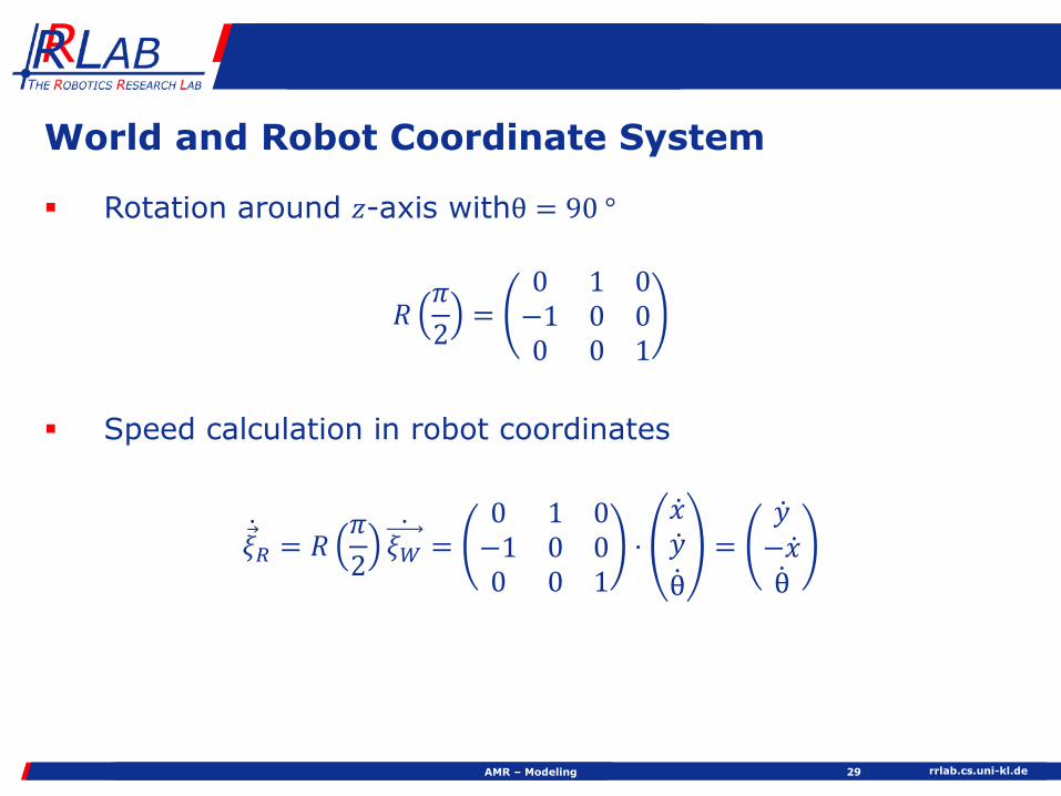

rrlabcsuni-klde
Vehicle Kinematics -
Analytical Solution
rrlabcsuni-kldeAMR ndash Kinematics 31
Control of the Test Vehicle GATOR
rrlabcsuni-kldeAMR ndash Kinematics 32
Forward kinematics for wheel driven robot
What is the robotrsquos trajectory if wheel geometry and speed are known
YW
XW
θ
V(t)
120596(t)
rrlabcsuni-kldeAMR ndash kinematics 33
Example Differential Drive
119903 radius of the wheel
119889 distance wheel center to kinematic center
ሶ120595119903 ሶ120595119897 Angular velocity of leftright wheel
ሶԦ120585119882 speed calculation in world coordinates
ሶԦ120585119882 = ሶ119909 ሶ119910 ሶ120579119879
= 119891 119889 119903 120579 ሶ120595119897 ሶ120595119903
= 119877 120579 minus1 ሶԦ120585119877
passive wheel
active wheel
d
rrlabcsuni-kldeAMR ndash Kinematics 34
Example Differential Drive
Calculation of the contribution of the left and right wheel to the speed along the longitudinal axis (119883119877)
Calculation of the contribution of the left and right wheel to the angular velocity of kinematic center
Summation of both results in the velocity and angular velocity along the 119883119877-axis where
ሶ119909119877119903 =119903 ሶ1205951199032
ሶ119909119877119897 =119903 ሶ120595119897
2
120596119903 =119903 ሶ1205951199032119889
120596119897 =minus119903 ሶ120595119897
2119889
ሶԦ120585119882 = 119877 120579 minus1 ሶԦ120585119903ሶԦ120585119903 =
119903 ሶ1205951199032
+119903 ሶ120595119897
2 0
119903 ሶ1205951199032119889
minus119903 ሶ120595119897
2119889
119879
rrlabcsuni-kldeAMR ndash Kinematics 35
Example Differential Drive
Since 119877 120579 is orthonormal
119877 120579 minus1 =cos 120579 minus sin 120579 0sin 120579 cos 120579 00 0 1
Given 120579 =120587
2 119903 = 1 119889 = 1 ሶ120595119903 = 4 ሶ120595119897 = 2 and wheel speed
notated in rounds per second 2120587
119904
ሶԦ120585119882 =ሶ119909ሶ119910ሶ120579
=0 minus1 01 0 00 0 1
sdot301
=031
rrlabcsuni-kldeAMR ndash Kinematics 36
Calculation of Wheel kinematics
Stepwise calculation of the linear and the rotational velocity for wheeled vehicles in 2D environment
Kinematic center moved with ሶ119909 ሶ119910 ሶ120579119879
Determine rotational velocity of each wheel
Collect all equations and solve the equation system
Consider
Equation system must no be solvable
No dynamic aspects will be considered
Calculation of the speed of the kinematic center based on thewheel speed can also be determined out of the equationsystem (inverse problem)
rrlabcsuni-klde
Basic Wheel Types
AMR ndash Kinematics 37
Standardwheel
Steerablestandard
wheel
Castorwheel
Swedish orMecanum
wheel
Ball orspherical
wheel
rrlabcsuni-kldeAMR ndash Kinematics 38
Wheel Properties
Standard and steerable wheel
Linear velocity along wheel plane ሶ119909 = 119903 ሶ120595
No sliding orthogonal to wheel plane ሶ119910 = 0
Castor wheel
Linear velocity along wheel plane ሶ119909 = 119903 ሶ120595
Linear perpendicular velocity ሶ119910 = minus119889119888 ሶ120573
SwedishMecanum wheel
Linear velocity along wheel plane ሶ119909 = 119903 ሶ120595 cos 120574
120574 angle of passive rollers (45 deg or 90 deg)
Linear perpendicular velocity ሶ119910 = 119903 ሶ120595 sin 120574 + 119903119901119903 ሶ120595119901119903
rrlabcsuni-kldeAMR ndash Kinematics 39
Kinematic Parameters
rrlabcsuni-kldeAMR ndash Kinematics 40
Kinematic Parameters
120572 Angle between 119909-axis and wheel mount point
120573 Angle between the straight line through the kinematic center and the fixing point of the wheel and the 119910-axis of the wheel frame
119889 Distance from the kinematic center to the wheel fixingpoint
119889119888 Distance from the wheel fixing point to the wheel supporting point (Castor wheel only)
120574 Angle between the 119909-axis of the wheel and rolling direction of the rollers (Mecanum wheel only)
rrlabcsuni-kldeAMR ndash Kinematics 41
Kinematic Parameters Standard Wheel
ሶ120595 119903
rrlabcsuni-kldeAMR ndash Kinematics 42
Kinematic Parameters Steerable Wheel
ሶ120595 119903
rrlabcsuni-kldeAMR ndash Kinematics 43
Kinematic Parameters Castor Wheel
ሶ120595 119903
rrlabcsuni-kldeAMR ndash Kinematics 44
Kinematic Parameters Mecanum Wheel
ሶ120595 119903
rrlabcsuni-kldeAMR ndash Kinematics 45
Kinematic Parameters Ball Wheel
ሶ120595 119903
rrlabcsuni-kldeAMR ndash Kinematics 46
Calculation of Wheel Velocity
Given velocity vector Ԧ119907 = ሶ119909 ሶ119910 ሶ120579119879
of the kinematic center
Calculation of linear velocity of standard wheel due to the speed of the kinematic center
Stepwise apply the following equations
Initial parameters 11205961 = 00 ሶ120579119879
and 1 Ԧ1199071 = ሶ119909 ሶ119910 0 119879
No additional rotational speed all 119894120596119894 = 00 ሶ120579119879
119894+1120596119894+1 = 119894119894+1119877 sdot 119894120596119894 + ሶ120579119894+1
119894+1 Ԧ119890119911119894+1
119894+1 Ԧ119907119894+1 = 119894119894+1119877 119894 Ԧ119907119894 +
119894120596119894 times119894 Ԧ119901119894+1
rrlabcsuni-kldeAMR ndash Kinematics 47
Calculation of Wheel Velocity
After the rotation around the 119911-axis with angle 120572 2 Ԧ1199072 is
calculated as
2 Ԧ1199072 =119888120572 ሶ119909 + 119904120572 ሶ119910minus119904120572 ሶ119909 + 119888120572 ሶ119910
0
Due to the translation 119889 3 Ԧ1199073 is
3 Ԧ1199073 =
119888120572 ሶ119909 + 119904120572 ሶ119910
minus119904120572 ሶ119909 + 119888120572 ሶ119910 + 119889 ሶ1205790
rrlabcsuni-kldeAMR ndash Kinematics 48
Calculation of Wheel Velocity
The last rotation around the 119911-axis with angle 120573 minus 90degtransfers the 119909-axis of the last frame to the rolling direction of the wheel
For the calculation of 4 Ԧ1199074 in the next equation
sin 120573 minus 90deg = minus cos120573 and cos 120573 minus 90deg = sin 120573 is used
4 Ԧ1199074 =119904 120572 + 120573 ሶ119909 minus 119888 120572 + 120573 ሶ119910 minus 119888120573 119889 ሶ120579
119888 120572 + 120573 ሶ119909 + 119904 120572 + 120573 ሶ119910 + 119904120573 119889 ሶ1205790
rrlabcsuni-kldeAMR ndash 4 Modeling 49
Calculation of Wheel Velocity
Last step is to equalize the linear velocity vector of the standard wheel to the velocity of the kinematic center represented in the wheel frame
119904 120572 + 120573 minus119888 120572 + 120573 minus119888120573 119889
119888 120572 + 120573 119904 120572 + 120573 119904120573 1198890 0 0
ሶ119909119910 ሶሶ120579
=119903 ሶ12059500
1st equation 119903 ሶ120595 = 119888 120572 + 120573 ሶ119909 + 119904 120572 + 120573 ሶ119910 + 119904120573 119889 ሶ120579 is called the
rolling constraint of the wheel because it describes the speed in the rolling direction of the wheel
2nd equation 119888 120572 + 120573 ሶ119909 + 119904 120572 + 120573 ሶ119910 + 119904120573 119889 ሶ120579 = 0 is called the
sliding constraint which describes the speed perpendicular to wheel plane
Sliding constraints are collected in Matrix 119878 ndash add row (119888(120572 +
rrlabcsuni-kldeAMR ndash Kinematics 50
Wheel Type-specific Velocity Vector
In case of the steerable standard wheel the fixed angle 120573 is replaced by a function 120573 119905
Equation could also be applied to the spherical wheel (based on the forces which affect the wheel and change 120573 119905 only a linear velocity in the rolling direction exists)
In case of castor wheels the y-component of the velocity
vector is depending on the angular velocity ሶ120573 and the length of the rod
119904 120572 + 120573(119905) minus119888 120572 + 120573(119905) minus119888120573(119905)119889
119888 120572 + 120573(119905) 119904 120572 + 120573(119905) 119904120573(119905)1198890 0 0
ሶ119909ሶ119910ሶ120579
=119903 ሶ120595
minus119889119888 ሶ120573(119905)0
Sliding constraints are collected in Matrix 119878 ndash add row 119888 120572 + 120573(119905) 119904 120572 + 120573(119905) 119904120573(119905)119889 (is used in section
maneuverability)
rrlabcsuni-kldeAMR ndash 4 Modeling 51
Wheel Type-specific Velocity Vector
Swedish or Mecanum wheel is able to move in an omnidirectional way
119904 120572 + 120573 + 120574 minus119888 120572 + 120573 + 120574 minus119888 120573 + 120574 119889
119888 120572 + 120573 + 120574 119904 120572 + 120573 + 120574 119904 120573 + 120574 1198890 0 0
ሶ119909ሶ119910ሶ120579
=119903 ሶ120595 cos 120574
119903 ሶ120595 sin 120574 + 119903119901119903 ሶ1205951199011199030
rrlabcsuni-kldeAMR ndash Kinematics 52
Vehicle Motion Calculation
Transformation of wheel velocities to velocity of kinematic center
Determine parameters 120572 120573 120574d indicating the wheel pose
Insert 120572 120573 120574 into appropriate wheel equation (as shown before) for each wheel
Solve system of equations
rrlabcsuni-kldeAMR ndash Kinematics 53
Differential Drive Kinematics
Two fixed standard wheels mounted on one axis
Kinematic center located in the middle of the axis
Distance between the kinematic center and each wheel 119889
Kinematic center is origin of coordinate frame
One solution for modeling the wheel configuration is to place the wheels on the 119910-axis
Kinematic parameters
120572119897 = 90 deg
120573119897 = 0 deg
120572119903 = minus90 deg
120573119903 = 180 deg
rrlabcsuni-kldeAMR ndash Kinematics 54
Differential Drive Kinematics
Apply equations for standard wheels (for the left and the right wheel)
119904 120572119897 + 120573119897 ሶ119909 minus 119888 120572119897 + 120573119897 ሶ119910 minus 119888120573119897 119889 ሶ120579 = 119903119897 ሶ120595119897
119888 120572119897 + 120573119897 ሶ119909 + 119904 120572119897 + 120573119897 ሶ119910 + 119904120573119897 119889 ሶ120579 = 0
119904 120572119903 + 120573119903 ሶ119909 minus 119888 120572119903 + 120573119903 ሶ119910 minus 119888120573119903 119889 ሶ120579 = 119903119903 ሶ120595119903119888 120572119903 + 120572119903 ሶ119909 + 119904 120572119903 + 120573119903 ሶ119910 + 119904120573119903 119889 ሶ120579 = 0
If the above mentioned parameters are inserted the following equations will result
ሶ119909 minus 119889 ሶ120579 = 119903119897 ሶ120595119897
ሶ119910 = 0
ሶ119909 + 119889 ሶ120579 = 119903119903 ሶ120595119903119910 = 0
rrlabcsuni-kldeAMR ndash Kinematics 55
Differential Drive Kinematics
Solving the system of equations yields
ሶ119909ሶ119910ሶ120579
=
1
2119903119897 ሶ120595119897 + 119903119903 ሶ120595119903
01
2119889minus119903119897 ሶ120595119897 + 119903119903 ሶ120595119903
rrlabcsuni-kldeAMR ndash Kinematics 56
Differential Drive Kinematics of MARVIN
rrlabcsuni-klde
CROMSCI ndash Equipped with 3 Steerable Standard Wheels
AMR ndash Kinematics 57
Climbing robot CROMSCI Wheel settings of CROMSCI
rrlabcsuni-klde
Omnidirectional Drive Kinematics
AMR ndash Kinematics 58
Typical orientations of the 3 steerable wheels of an omnidirectional vehicle
rrlabcsuni-kldeAMR ndash Kinematicsg 59
Omnidirectional Drive Kinematics
Three steerable standard wheels
Kinematic center located in the middle of the robot
Distance between the kinematic center and each wheel 119889
Origin of coordinates frame is kinematic center
Kinematic parameters
1205721 = 0 deg
1205722 = 120 deg
1205723 = minus120 deg
rrlabcsuni-kldeAMR ndash Kinematics 60
Omnidirectional Drive Kinematics
Applying equation for steerable standard wheel for each wheel leads to the following system of equations
119904 1205721 + 1205731 ሶ119909 minus 119888 1205721 + 1205731 ሶ119910 minus 119889 sdot 119888 1205731 ሶ120579 = 1199031 ሶ1205951
119904 1205722 + 1205732 ሶ119909 minus 119888 1205722 + 1205732 ሶ119910 minus 119889 sdot 119888 1205732 ሶ120579 = 1199032 ሶ1205952
119904 1205723 + 1205733 ሶ119909 minus 119888 1205723 + 1205733 ሶ119910 minus 119889 sdot 119888 1205733 ሶ120579 = 1199033 ሶ1205953
119888 1205721 + 1205731 ሶ119909 + 119904 1205721 + 1205731 ሶ119910 + 119889 sdot 119904 1205731 ሶ120579 = 0
119888 1205722 + 1205732 ሶ119909 + 119904 1205722 + 1205732 ሶ119910 + 119889 sdot 119904 1205732 ሶ120579 = 0
119888 1205723 + 1205733 ሶ119909 + 119904 1205723 + 1205733 ሶ119910 + 119889 sdot 119904 1205733 ሶ120579 = 0
rrlabcsuni-kldeAMR ndash Kinematics 61
Omnidirectional Drive Kinematics
Based on these equation the steering angles 120573119894 119894 = 123 can be determined
119888 120572119894 + 120573119894 sdot ሶ119909 + 119904 120572119894 + 120573119894 sdot ሶ119910 + 119889 sdot 119904 120573119894 sdot ሶ120579 = 0
119888 120572119894 sdot 119888 120573119894 sdot ሶ119909 minus 119904 120572119894 sdot 119904 120573119894 sdot ሶ119909 + 119904 120572119894 sdot 119888 120573119894 sdot ሶ119910 + 119888 120572119894 sdot 119904 120573119894 sdot ሶ119910 + 119889 sdot 119904 120573119894 sdot ሶ120579 = 0
119888 120573119894 sdot 119888 120572119894 sdot ሶ119909 + 119904 120572119894 sdot ሶ119910 minus 119904 120573119894 sdot 119904 120572119894 sdot ሶ119909 minus 119888 120572119894 sdot ሶ119910 minus 119889 sdot ሶ120579 = 0
119888 120572119894 sdot ሶ119909 + 119904 120572119894 sdot ሶ119910
119904 120572119894 sdot ሶ119909 minus 119888 120572119894 sdot ሶ119910 minus 119889 sdot ሶ120579=119904 120573119894119888 120573119894
atan2 119888 120572119894 sdot ሶ119909 + 119904 120572119894 sdot ሶ119910 119904 120572119894 sdot ሶ119909 minus 119888 120572119894 sdot ሶ119910 minus 119889 sdot ሶ120579 = 120573119894
Also the angular velocity of the wheel ሶ120595119894 can now be calculated
ሶ120595119894 =1
119903119894119904 120572119894 + 120573119894 ሶ119909 minus 119888 120572119894 + 120573119894 ሶ119910 minus 119889 sdot 119888 120573119894 ሶ120579
rrlabcsuni-klde
The Climbing Robot CROMSCI
AMR ndash Kinematics 62
rrlabcsuni-klde
Mecanum Vehicle
AMR ndash Kinematics 63
Schematic configurationof a Mecanum wheel(Viewed from above)
The mobile robot PRIAMOS of the University of Karlsruhe driven by Mecanum wheels
rrlabcsuni-kldeAMR ndash Kinematics 64
Mecanum Kinematics
To set up the kinematic equation first the parameters 120572 120573 120574for each wheel must be determined
The parameters for four wheels are
1205721 = 45 deg 1205731 = 45 deg 1205741 = minus45 deg
1205722 = 135 deg 1205732 = minus45 deg 1205742 = 45 deg
1205723 = minus135 deg 1205733 = 225 deg 1205743 = minus45 deg
1205724 = minus45 deg 1205734 = 135 deg 1205744 = 45 deg
rrlabcsuni-kldeAMR ndash Kinematics 65
Mecanum Kinematics
Assume all driven wheels have the same radius 119903 the same distance 119889 from the kinematic center and the above mentioned parameters 120572 120573 120574
Using equation for Mecanum wheels leads to equations
119904 45 deg ሶ119909 minus 119888 45 deg ሶ119910 minus 119889 ሶ120579 = 119903 sdot 119888 minus45 deg ሶ1205951
119904 135 deg ሶ119909 minus 119888 135 deg ሶ119910 minus 119889 ሶ120579 = 119903 sdot 119888 45 deg ሶ1205952
119904 45 deg ሶ119909 minus 119888 45 deg ሶ119910 minus 119889 ሶ120579 = 119903 sdot 119888 minus45 deg ሶ1205953
119904 135 deg ሶ119909 minus 119888 135 deg ሶ119910 minus 119889 ሶ120579 = 119903 sdot 119888 45 deg ሶ1205954
rrlabcsuni-kldeAMR ndash Kinematics 66
Mecanum Kinematics
The velocities ሶ119909 ሶ119910 ሶ120579 of the kinematic center can be calculated
ሶ119909 =119903
4ሶ1205951 + ሶ1205952 + ሶ1205953 + ሶ1205954
ሶ119910 =119903
4minus ሶ1205951 + ሶ1205952 minus ሶ1205953 + ሶ1205954
ሶ120579 =119903
119889 2ሶ1205951 minus ሶ1205952 minus ሶ1205953 + ሶ1205954
rrlabcsuni-kldeAMR ndash Kinematics 67
Mecanum Kinematics
The velocity vector of the kinematic center can be determined as
ሶ119909ሶ119910ሶ120579
=119903119908ℎ1198901198901198974
sdot1 1 1 1minus1 1 minus1 1119886 minus119886 minus119886 119886
sdot
ሶ1205951
ሶ1205952
ሶ1205953
ሶ1205954
with a =2 2
119889
Assuming the absence of slip the following must hold
ሶ1205954 = ሶ1205951 + ሶ1205952 minus ሶ1205953
rrlabcsuni-klde
Maneuverability of AMRs
rrlabcsuni-kldeAMR ndash Maneuverability 69
Choice of Wheel Configuration
Choice of wheels and their configuration depends on hellip
Ability to maneuver
Controllability
Stability
An optimum can only be achieved concerning a specific application
rrlabcsuni-kldeAMR ndash Maneuverability 70
Stability
Minimal number of wheels for static stability is 2 if center of gravity is located under the wheel axis (e g robot Cye)
Under standard conditions itrsquos 3
If more than 3 wheels are present adjustment to rough terrain becomes necessary
Typical setups
2 driven wheels on a single axis with 1 or 2 passive castor wheels
Single driven and steered wheel with two passive fixed wheels
rrlabcsuni-kldeAMR ndash Maneuverability 71
Maneuverability
Robotrsquos degree of freedom (DOF)
Outstanding ability to maneuver when the only driven wheel can be rotated in an active way
Example Ackermann steering
Poor ability to maneuver
5 m radius required for single rotation of a car
Lateral movement only possible troughforwardbackward movement
rrlabcsuni-kldeAMR ndash Maneuverability 72
Controllability
Costs for locomotion of the robot on a given trajectory
Contradiction to the robotrsquos ability to maneuver
Examples
Ackermann steering easy to control
Mecanum wheels very costly if high precision is required
Costs for controllability depend on hellip
Wheel type
Drive geometry
Sensors to determine driving situation
Motortransmission
rrlabcsuni-kldeAMR ndash Maneuverability 73
Degree of Mobility
The degree of mobility 119891119898 isin 123 points out how the sliding constraints (defined in Matrix 119878 see slide 42) affect the
possibilities for robot movement 119877 120579 ሶ120585119897 The mobility can be calculated by using the rank of the
matrix of sliding constraints of all standard wheels (steerable and fixed wheels) = number of independent constraints
119891119898 = 3 minus rank 119878
rrlabcsuni-kldeAMR ndash Maneuverability 74
Degree of Mobility
Example Differential Drive
Given only two fixed wheels geometrically we can set
1198891 = 1198892 1205731 = 1205732 = 0 1205721 + 120587 = 1205722
Matrix 119878 has two sliding constraints of the form (119888(120572 +
rrlabcsuni-kldeAMR ndash Maneuverability 75
Degree of Steerability
The degree of steerability 119891119904 isin 012 quantifies the degree of controllable freedom and is determined via the number of independently controllable steering parameters
Define 119878prime Part of 119878 defining sliding constraints of steerable wheels
119891119904 = rank 119878prime
More possibilities in steering will result in lower mobility
119891119904 = 0 No steered wheel (differential drive)
119891119904 = 1 At least one steered wheel (Ackermann steering)
119891119904 = 2 At least two steered wheels no fixed wheel
rrlabcsuni-kldeAMR ndash Maneuverability 76
Degree of Maneuverability
The degree of maneuverability 119891119872 isin 23 points out the number of DOF the robot can manipulate
119891119872 = 119891119898 + 119891119904
rrlabcsuni-klde
Vehicle Kinematics
Geometrical Solution
rrlabcsuni-kldeAMR ndash Kinematics 78
Tricycle Drive
Given 120575 119907
Unknown 119907prime 119907119897 119907119903 Solution
119903 = 119897 sdot cot 120575
119907prime =119907
cos 120575
119907119897 = 119907 sdot119903 + 119889
119903
119907119903 = 119907 sdot119903 minus 119889
119903 Tricycle drive kinematics
120575
rrlabcsuni-kldeAMR ndash 4 Kinematics 79
Ackermann Steering
Given 119907119863 120575 119897 119889
Unknown 119907119903119903 119907119897119903 119907119903119891 119907119897119891
Solution
120602 =119897
tan 120575
119907119897119903 =120602 minus 1198892 sdot 119907119863
120602
119907119903119903 =120602 + 1198892 sdot 119907119863
120602
119907119897119891 =120602 minus 1198892 2 + 1198972 sdot tan 120575
119897sdot 119907119863
119907119903119891 =1206022 + 1198972 sdot tan 120575
119897sdot 119907119863
Kinematics ofAckermann steering
120575
120602
rrlabcsuni-klde
Omnidrive Kinematics
AMR ndash Kinematics 80
Given 120602 120593 119907 119889
Unknown 1205931 1205932 1199071 1199072 Solution
120549119909 = 120602 sdot cos120593120549119910 = 120602 sdot sin1205931205931 = arctan120549119910 minus 1198891205491199091206021 = 120602 sdot cos120593 cos12059311199071 = 119907 sdot 1206021120602
1205932 = arctan120549119910 + 119889
1205491199091206022 = 120602 sdot cos120593 cos1205932
1199072 = 119907 sdot 1206022120602
120549119910 = 120602 ∙ 119904119894119899 120593
1205931
1205932
1206021
1206022
120593 120549119909 = 120602 ∙ cos120593
120602
119889
rrlabcsuni-klde
Bicycle Model
AMR ndash Kinematics 81
119907
rrlabcsuni-kldeAMR ndash Kinematics 82
Bicycle Model
Circular road of radius 120602
Low speed motion
Slip angles at both wheels are zero
Small total lateral force from both tires
119865119910 =1198981199072
120602
Point 119875 is instantaneous rolling center
Velocity at 119862 is perpendicular to line 119875119862
Heading angle 120579
Slip angle 120575119907 Course angle 120574 = 120579 + 120575119907
rrlabcsuni-kldeAMR ndash 4 Modeling 83
Bicycle Model
Given 120575119891 120575119903 119907 120579
Unknown ሶ119883 ሶ119884 ሶ120579
Solution
120575119907 = tanminus1119897119891 tan 120575119903+119897119903 tan 120575119891
119897119891+119897119903
ሶ120579 =119907
120602
120602 =119897119891+119897119903
tan 120575119891 minustan 120575119903 cos 120575119907
ሶ119883 = 119907 cos 120579 + 120575119907ሶ119884 = 119907 sin 120579 + 120575119907
ሶ120579 =119907 cos 120575119907
119897119891+119897119903tan 120575119891 minus tan 120575119903
119907
rrlabcsuni-klde
Ackermann Steering -gt Bicycle Model
AMR ndash Kinematics 84
119862 = 119874 120575119903 = 0 120575119891 = 120575
119897119903 = 0 119897119891 = 119897
120575119907 = 0
ሶ120579 =119907
120602
120602 =119897
tan 120575119891
ሶ119883 = 119907 cos 120579ሶ119884 = 119907 sin 120579ሶ120579 =
119907
119897119891tan 120575119891
119907
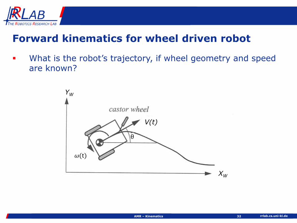
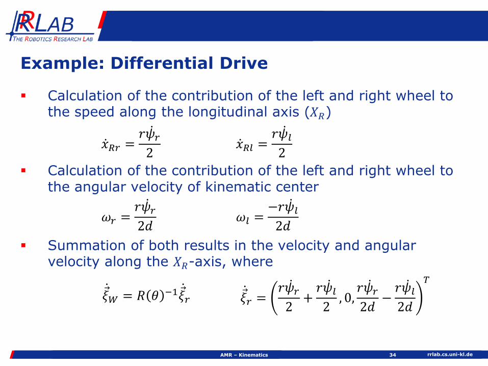

rrlabcsuni-klde
Basic Wheel Types
AMR ndash Kinematics 37
Standardwheel
Steerablestandard
wheel
Castorwheel
Swedish orMecanum
wheel
Ball orspherical
wheel
rrlabcsuni-kldeAMR ndash Kinematics 38
Wheel Properties
Standard and steerable wheel
Linear velocity along wheel plane ሶ119909 = 119903 ሶ120595
No sliding orthogonal to wheel plane ሶ119910 = 0
Castor wheel
Linear velocity along wheel plane ሶ119909 = 119903 ሶ120595
Linear perpendicular velocity ሶ119910 = minus119889119888 ሶ120573
SwedishMecanum wheel
Linear velocity along wheel plane ሶ119909 = 119903 ሶ120595 cos 120574
120574 angle of passive rollers (45 deg or 90 deg)
Linear perpendicular velocity ሶ119910 = 119903 ሶ120595 sin 120574 + 119903119901119903 ሶ120595119901119903
rrlabcsuni-kldeAMR ndash Kinematics 39
Kinematic Parameters
rrlabcsuni-kldeAMR ndash Kinematics 40
Kinematic Parameters
120572 Angle between 119909-axis and wheel mount point
120573 Angle between the straight line through the kinematic center and the fixing point of the wheel and the 119910-axis of the wheel frame
119889 Distance from the kinematic center to the wheel fixingpoint
119889119888 Distance from the wheel fixing point to the wheel supporting point (Castor wheel only)
120574 Angle between the 119909-axis of the wheel and rolling direction of the rollers (Mecanum wheel only)
rrlabcsuni-kldeAMR ndash Kinematics 41
Kinematic Parameters Standard Wheel
ሶ120595 119903
rrlabcsuni-kldeAMR ndash Kinematics 42
Kinematic Parameters Steerable Wheel
ሶ120595 119903
rrlabcsuni-kldeAMR ndash Kinematics 43
Kinematic Parameters Castor Wheel
ሶ120595 119903
rrlabcsuni-kldeAMR ndash Kinematics 44
Kinematic Parameters Mecanum Wheel
ሶ120595 119903
rrlabcsuni-kldeAMR ndash Kinematics 45
Kinematic Parameters Ball Wheel
ሶ120595 119903
rrlabcsuni-kldeAMR ndash Kinematics 46
Calculation of Wheel Velocity
Given velocity vector Ԧ119907 = ሶ119909 ሶ119910 ሶ120579119879
of the kinematic center
Calculation of linear velocity of standard wheel due to the speed of the kinematic center
Stepwise apply the following equations
Initial parameters 11205961 = 00 ሶ120579119879
and 1 Ԧ1199071 = ሶ119909 ሶ119910 0 119879
No additional rotational speed all 119894120596119894 = 00 ሶ120579119879
119894+1120596119894+1 = 119894119894+1119877 sdot 119894120596119894 + ሶ120579119894+1
119894+1 Ԧ119890119911119894+1
119894+1 Ԧ119907119894+1 = 119894119894+1119877 119894 Ԧ119907119894 +
119894120596119894 times119894 Ԧ119901119894+1
rrlabcsuni-kldeAMR ndash Kinematics 47
Calculation of Wheel Velocity
After the rotation around the 119911-axis with angle 120572 2 Ԧ1199072 is
calculated as
2 Ԧ1199072 =119888120572 ሶ119909 + 119904120572 ሶ119910minus119904120572 ሶ119909 + 119888120572 ሶ119910
0
Due to the translation 119889 3 Ԧ1199073 is
3 Ԧ1199073 =
119888120572 ሶ119909 + 119904120572 ሶ119910
minus119904120572 ሶ119909 + 119888120572 ሶ119910 + 119889 ሶ1205790
rrlabcsuni-kldeAMR ndash Kinematics 48
Calculation of Wheel Velocity
The last rotation around the 119911-axis with angle 120573 minus 90degtransfers the 119909-axis of the last frame to the rolling direction of the wheel
For the calculation of 4 Ԧ1199074 in the next equation
sin 120573 minus 90deg = minus cos120573 and cos 120573 minus 90deg = sin 120573 is used
4 Ԧ1199074 =119904 120572 + 120573 ሶ119909 minus 119888 120572 + 120573 ሶ119910 minus 119888120573 119889 ሶ120579
119888 120572 + 120573 ሶ119909 + 119904 120572 + 120573 ሶ119910 + 119904120573 119889 ሶ1205790
rrlabcsuni-kldeAMR ndash 4 Modeling 49
Calculation of Wheel Velocity
Last step is to equalize the linear velocity vector of the standard wheel to the velocity of the kinematic center represented in the wheel frame
119904 120572 + 120573 minus119888 120572 + 120573 minus119888120573 119889
119888 120572 + 120573 119904 120572 + 120573 119904120573 1198890 0 0
ሶ119909119910 ሶሶ120579
=119903 ሶ12059500
1st equation 119903 ሶ120595 = 119888 120572 + 120573 ሶ119909 + 119904 120572 + 120573 ሶ119910 + 119904120573 119889 ሶ120579 is called the
rolling constraint of the wheel because it describes the speed in the rolling direction of the wheel
2nd equation 119888 120572 + 120573 ሶ119909 + 119904 120572 + 120573 ሶ119910 + 119904120573 119889 ሶ120579 = 0 is called the
sliding constraint which describes the speed perpendicular to wheel plane
Sliding constraints are collected in Matrix 119878 ndash add row (119888(120572 +
rrlabcsuni-kldeAMR ndash Kinematics 50
Wheel Type-specific Velocity Vector
In case of the steerable standard wheel the fixed angle 120573 is replaced by a function 120573 119905
Equation could also be applied to the spherical wheel (based on the forces which affect the wheel and change 120573 119905 only a linear velocity in the rolling direction exists)
In case of castor wheels the y-component of the velocity
vector is depending on the angular velocity ሶ120573 and the length of the rod
119904 120572 + 120573(119905) minus119888 120572 + 120573(119905) minus119888120573(119905)119889
119888 120572 + 120573(119905) 119904 120572 + 120573(119905) 119904120573(119905)1198890 0 0
ሶ119909ሶ119910ሶ120579
=119903 ሶ120595
minus119889119888 ሶ120573(119905)0
Sliding constraints are collected in Matrix 119878 ndash add row 119888 120572 + 120573(119905) 119904 120572 + 120573(119905) 119904120573(119905)119889 (is used in section
maneuverability)
rrlabcsuni-kldeAMR ndash 4 Modeling 51
Wheel Type-specific Velocity Vector
Swedish or Mecanum wheel is able to move in an omnidirectional way
119904 120572 + 120573 + 120574 minus119888 120572 + 120573 + 120574 minus119888 120573 + 120574 119889
119888 120572 + 120573 + 120574 119904 120572 + 120573 + 120574 119904 120573 + 120574 1198890 0 0
ሶ119909ሶ119910ሶ120579
=119903 ሶ120595 cos 120574
119903 ሶ120595 sin 120574 + 119903119901119903 ሶ1205951199011199030
rrlabcsuni-kldeAMR ndash Kinematics 52
Vehicle Motion Calculation
Transformation of wheel velocities to velocity of kinematic center
Determine parameters 120572 120573 120574d indicating the wheel pose
Insert 120572 120573 120574 into appropriate wheel equation (as shown before) for each wheel
Solve system of equations
rrlabcsuni-kldeAMR ndash Kinematics 53
Differential Drive Kinematics
Two fixed standard wheels mounted on one axis
Kinematic center located in the middle of the axis
Distance between the kinematic center and each wheel 119889
Kinematic center is origin of coordinate frame
One solution for modeling the wheel configuration is to place the wheels on the 119910-axis
Kinematic parameters
120572119897 = 90 deg
120573119897 = 0 deg
120572119903 = minus90 deg
120573119903 = 180 deg
rrlabcsuni-kldeAMR ndash Kinematics 54
Differential Drive Kinematics
Apply equations for standard wheels (for the left and the right wheel)
119904 120572119897 + 120573119897 ሶ119909 minus 119888 120572119897 + 120573119897 ሶ119910 minus 119888120573119897 119889 ሶ120579 = 119903119897 ሶ120595119897
119888 120572119897 + 120573119897 ሶ119909 + 119904 120572119897 + 120573119897 ሶ119910 + 119904120573119897 119889 ሶ120579 = 0
119904 120572119903 + 120573119903 ሶ119909 minus 119888 120572119903 + 120573119903 ሶ119910 minus 119888120573119903 119889 ሶ120579 = 119903119903 ሶ120595119903119888 120572119903 + 120572119903 ሶ119909 + 119904 120572119903 + 120573119903 ሶ119910 + 119904120573119903 119889 ሶ120579 = 0
If the above mentioned parameters are inserted the following equations will result
ሶ119909 minus 119889 ሶ120579 = 119903119897 ሶ120595119897
ሶ119910 = 0
ሶ119909 + 119889 ሶ120579 = 119903119903 ሶ120595119903119910 = 0
rrlabcsuni-kldeAMR ndash Kinematics 55
Differential Drive Kinematics
Solving the system of equations yields
ሶ119909ሶ119910ሶ120579
=
1
2119903119897 ሶ120595119897 + 119903119903 ሶ120595119903
01
2119889minus119903119897 ሶ120595119897 + 119903119903 ሶ120595119903
rrlabcsuni-kldeAMR ndash Kinematics 56
Differential Drive Kinematics of MARVIN
rrlabcsuni-klde
CROMSCI ndash Equipped with 3 Steerable Standard Wheels
AMR ndash Kinematics 57
Climbing robot CROMSCI Wheel settings of CROMSCI
rrlabcsuni-klde
Omnidirectional Drive Kinematics
AMR ndash Kinematics 58
Typical orientations of the 3 steerable wheels of an omnidirectional vehicle
rrlabcsuni-kldeAMR ndash Kinematicsg 59
Omnidirectional Drive Kinematics
Three steerable standard wheels
Kinematic center located in the middle of the robot
Distance between the kinematic center and each wheel 119889
Origin of coordinates frame is kinematic center
Kinematic parameters
1205721 = 0 deg
1205722 = 120 deg
1205723 = minus120 deg
rrlabcsuni-kldeAMR ndash Kinematics 60
Omnidirectional Drive Kinematics
Applying equation for steerable standard wheel for each wheel leads to the following system of equations
119904 1205721 + 1205731 ሶ119909 minus 119888 1205721 + 1205731 ሶ119910 minus 119889 sdot 119888 1205731 ሶ120579 = 1199031 ሶ1205951
119904 1205722 + 1205732 ሶ119909 minus 119888 1205722 + 1205732 ሶ119910 minus 119889 sdot 119888 1205732 ሶ120579 = 1199032 ሶ1205952
119904 1205723 + 1205733 ሶ119909 minus 119888 1205723 + 1205733 ሶ119910 minus 119889 sdot 119888 1205733 ሶ120579 = 1199033 ሶ1205953
119888 1205721 + 1205731 ሶ119909 + 119904 1205721 + 1205731 ሶ119910 + 119889 sdot 119904 1205731 ሶ120579 = 0
119888 1205722 + 1205732 ሶ119909 + 119904 1205722 + 1205732 ሶ119910 + 119889 sdot 119904 1205732 ሶ120579 = 0
119888 1205723 + 1205733 ሶ119909 + 119904 1205723 + 1205733 ሶ119910 + 119889 sdot 119904 1205733 ሶ120579 = 0
rrlabcsuni-kldeAMR ndash Kinematics 61
Omnidirectional Drive Kinematics
Based on these equation the steering angles 120573119894 119894 = 123 can be determined
119888 120572119894 + 120573119894 sdot ሶ119909 + 119904 120572119894 + 120573119894 sdot ሶ119910 + 119889 sdot 119904 120573119894 sdot ሶ120579 = 0
119888 120572119894 sdot 119888 120573119894 sdot ሶ119909 minus 119904 120572119894 sdot 119904 120573119894 sdot ሶ119909 + 119904 120572119894 sdot 119888 120573119894 sdot ሶ119910 + 119888 120572119894 sdot 119904 120573119894 sdot ሶ119910 + 119889 sdot 119904 120573119894 sdot ሶ120579 = 0
119888 120573119894 sdot 119888 120572119894 sdot ሶ119909 + 119904 120572119894 sdot ሶ119910 minus 119904 120573119894 sdot 119904 120572119894 sdot ሶ119909 minus 119888 120572119894 sdot ሶ119910 minus 119889 sdot ሶ120579 = 0
119888 120572119894 sdot ሶ119909 + 119904 120572119894 sdot ሶ119910
119904 120572119894 sdot ሶ119909 minus 119888 120572119894 sdot ሶ119910 minus 119889 sdot ሶ120579=119904 120573119894119888 120573119894
atan2 119888 120572119894 sdot ሶ119909 + 119904 120572119894 sdot ሶ119910 119904 120572119894 sdot ሶ119909 minus 119888 120572119894 sdot ሶ119910 minus 119889 sdot ሶ120579 = 120573119894
Also the angular velocity of the wheel ሶ120595119894 can now be calculated
ሶ120595119894 =1
119903119894119904 120572119894 + 120573119894 ሶ119909 minus 119888 120572119894 + 120573119894 ሶ119910 minus 119889 sdot 119888 120573119894 ሶ120579
rrlabcsuni-klde
The Climbing Robot CROMSCI
AMR ndash Kinematics 62
rrlabcsuni-klde
Mecanum Vehicle
AMR ndash Kinematics 63
Schematic configurationof a Mecanum wheel(Viewed from above)
The mobile robot PRIAMOS of the University of Karlsruhe driven by Mecanum wheels
rrlabcsuni-kldeAMR ndash Kinematics 64
Mecanum Kinematics
To set up the kinematic equation first the parameters 120572 120573 120574for each wheel must be determined
The parameters for four wheels are
1205721 = 45 deg 1205731 = 45 deg 1205741 = minus45 deg
1205722 = 135 deg 1205732 = minus45 deg 1205742 = 45 deg
1205723 = minus135 deg 1205733 = 225 deg 1205743 = minus45 deg
1205724 = minus45 deg 1205734 = 135 deg 1205744 = 45 deg
rrlabcsuni-kldeAMR ndash Kinematics 65
Mecanum Kinematics
Assume all driven wheels have the same radius 119903 the same distance 119889 from the kinematic center and the above mentioned parameters 120572 120573 120574
Using equation for Mecanum wheels leads to equations
119904 45 deg ሶ119909 minus 119888 45 deg ሶ119910 minus 119889 ሶ120579 = 119903 sdot 119888 minus45 deg ሶ1205951
119904 135 deg ሶ119909 minus 119888 135 deg ሶ119910 minus 119889 ሶ120579 = 119903 sdot 119888 45 deg ሶ1205952
119904 45 deg ሶ119909 minus 119888 45 deg ሶ119910 minus 119889 ሶ120579 = 119903 sdot 119888 minus45 deg ሶ1205953
119904 135 deg ሶ119909 minus 119888 135 deg ሶ119910 minus 119889 ሶ120579 = 119903 sdot 119888 45 deg ሶ1205954
rrlabcsuni-kldeAMR ndash Kinematics 66
Mecanum Kinematics
The velocities ሶ119909 ሶ119910 ሶ120579 of the kinematic center can be calculated
ሶ119909 =119903
4ሶ1205951 + ሶ1205952 + ሶ1205953 + ሶ1205954
ሶ119910 =119903
4minus ሶ1205951 + ሶ1205952 minus ሶ1205953 + ሶ1205954
ሶ120579 =119903
119889 2ሶ1205951 minus ሶ1205952 minus ሶ1205953 + ሶ1205954
rrlabcsuni-kldeAMR ndash Kinematics 67
Mecanum Kinematics
The velocity vector of the kinematic center can be determined as
ሶ119909ሶ119910ሶ120579
=119903119908ℎ1198901198901198974
sdot1 1 1 1minus1 1 minus1 1119886 minus119886 minus119886 119886
sdot
ሶ1205951
ሶ1205952
ሶ1205953
ሶ1205954
with a =2 2
119889
Assuming the absence of slip the following must hold
ሶ1205954 = ሶ1205951 + ሶ1205952 minus ሶ1205953
rrlabcsuni-klde
Maneuverability of AMRs
rrlabcsuni-kldeAMR ndash Maneuverability 69
Choice of Wheel Configuration
Choice of wheels and their configuration depends on hellip
Ability to maneuver
Controllability
Stability
An optimum can only be achieved concerning a specific application
rrlabcsuni-kldeAMR ndash Maneuverability 70
Stability
Minimal number of wheels for static stability is 2 if center of gravity is located under the wheel axis (e g robot Cye)
Under standard conditions itrsquos 3
If more than 3 wheels are present adjustment to rough terrain becomes necessary
Typical setups
2 driven wheels on a single axis with 1 or 2 passive castor wheels
Single driven and steered wheel with two passive fixed wheels
rrlabcsuni-kldeAMR ndash Maneuverability 71
Maneuverability
Robotrsquos degree of freedom (DOF)
Outstanding ability to maneuver when the only driven wheel can be rotated in an active way
Example Ackermann steering
Poor ability to maneuver
5 m radius required for single rotation of a car
Lateral movement only possible troughforwardbackward movement
rrlabcsuni-kldeAMR ndash Maneuverability 72
Controllability
Costs for locomotion of the robot on a given trajectory
Contradiction to the robotrsquos ability to maneuver
Examples
Ackermann steering easy to control
Mecanum wheels very costly if high precision is required
Costs for controllability depend on hellip
Wheel type
Drive geometry
Sensors to determine driving situation
Motortransmission
rrlabcsuni-kldeAMR ndash Maneuverability 73
Degree of Mobility
The degree of mobility 119891119898 isin 123 points out how the sliding constraints (defined in Matrix 119878 see slide 42) affect the
possibilities for robot movement 119877 120579 ሶ120585119897 The mobility can be calculated by using the rank of the
matrix of sliding constraints of all standard wheels (steerable and fixed wheels) = number of independent constraints
119891119898 = 3 minus rank 119878
rrlabcsuni-kldeAMR ndash Maneuverability 74
Degree of Mobility
Example Differential Drive
Given only two fixed wheels geometrically we can set
1198891 = 1198892 1205731 = 1205732 = 0 1205721 + 120587 = 1205722
Matrix 119878 has two sliding constraints of the form (119888(120572 +
rrlabcsuni-kldeAMR ndash Maneuverability 75
Degree of Steerability
The degree of steerability 119891119904 isin 012 quantifies the degree of controllable freedom and is determined via the number of independently controllable steering parameters
Define 119878prime Part of 119878 defining sliding constraints of steerable wheels
119891119904 = rank 119878prime
More possibilities in steering will result in lower mobility
119891119904 = 0 No steered wheel (differential drive)
119891119904 = 1 At least one steered wheel (Ackermann steering)
119891119904 = 2 At least two steered wheels no fixed wheel
rrlabcsuni-kldeAMR ndash Maneuverability 76
Degree of Maneuverability
The degree of maneuverability 119891119872 isin 23 points out the number of DOF the robot can manipulate
119891119872 = 119891119898 + 119891119904
rrlabcsuni-klde
Vehicle Kinematics
Geometrical Solution
rrlabcsuni-kldeAMR ndash Kinematics 78
Tricycle Drive
Given 120575 119907
Unknown 119907prime 119907119897 119907119903 Solution
119903 = 119897 sdot cot 120575
119907prime =119907
cos 120575
119907119897 = 119907 sdot119903 + 119889
119903
119907119903 = 119907 sdot119903 minus 119889
119903 Tricycle drive kinematics
120575
rrlabcsuni-kldeAMR ndash 4 Kinematics 79
Ackermann Steering
Given 119907119863 120575 119897 119889
Unknown 119907119903119903 119907119897119903 119907119903119891 119907119897119891
Solution
120602 =119897
tan 120575
119907119897119903 =120602 minus 1198892 sdot 119907119863
120602
119907119903119903 =120602 + 1198892 sdot 119907119863
120602
119907119897119891 =120602 minus 1198892 2 + 1198972 sdot tan 120575
119897sdot 119907119863
119907119903119891 =1206022 + 1198972 sdot tan 120575
119897sdot 119907119863
Kinematics ofAckermann steering
120575
120602
rrlabcsuni-klde
Omnidrive Kinematics
AMR ndash Kinematics 80
Given 120602 120593 119907 119889
Unknown 1205931 1205932 1199071 1199072 Solution
120549119909 = 120602 sdot cos120593120549119910 = 120602 sdot sin1205931205931 = arctan120549119910 minus 1198891205491199091206021 = 120602 sdot cos120593 cos12059311199071 = 119907 sdot 1206021120602
1205932 = arctan120549119910 + 119889
1205491199091206022 = 120602 sdot cos120593 cos1205932
1199072 = 119907 sdot 1206022120602
120549119910 = 120602 ∙ 119904119894119899 120593
1205931
1205932
1206021
1206022
120593 120549119909 = 120602 ∙ cos120593
120602
119889
rrlabcsuni-klde
Bicycle Model
AMR ndash Kinematics 81
119907
rrlabcsuni-kldeAMR ndash Kinematics 82
Bicycle Model
Circular road of radius 120602
Low speed motion
Slip angles at both wheels are zero
Small total lateral force from both tires
119865119910 =1198981199072
120602
Point 119875 is instantaneous rolling center
Velocity at 119862 is perpendicular to line 119875119862
Heading angle 120579
Slip angle 120575119907 Course angle 120574 = 120579 + 120575119907
rrlabcsuni-kldeAMR ndash 4 Modeling 83
Bicycle Model
Given 120575119891 120575119903 119907 120579
Unknown ሶ119883 ሶ119884 ሶ120579
Solution
120575119907 = tanminus1119897119891 tan 120575119903+119897119903 tan 120575119891
119897119891+119897119903
ሶ120579 =119907
120602
120602 =119897119891+119897119903
tan 120575119891 minustan 120575119903 cos 120575119907
ሶ119883 = 119907 cos 120579 + 120575119907ሶ119884 = 119907 sin 120579 + 120575119907
ሶ120579 =119907 cos 120575119907
119897119891+119897119903tan 120575119891 minus tan 120575119903
119907
rrlabcsuni-klde
Ackermann Steering -gt Bicycle Model
AMR ndash Kinematics 84
119862 = 119874 120575119903 = 0 120575119891 = 120575
119897119903 = 0 119897119891 = 119897
120575119907 = 0
ሶ120579 =119907
120602
120602 =119897
tan 120575119891
ሶ119883 = 119907 cos 120579ሶ119884 = 119907 sin 120579ሶ120579 =
119907
119897119891tan 120575119891
119907
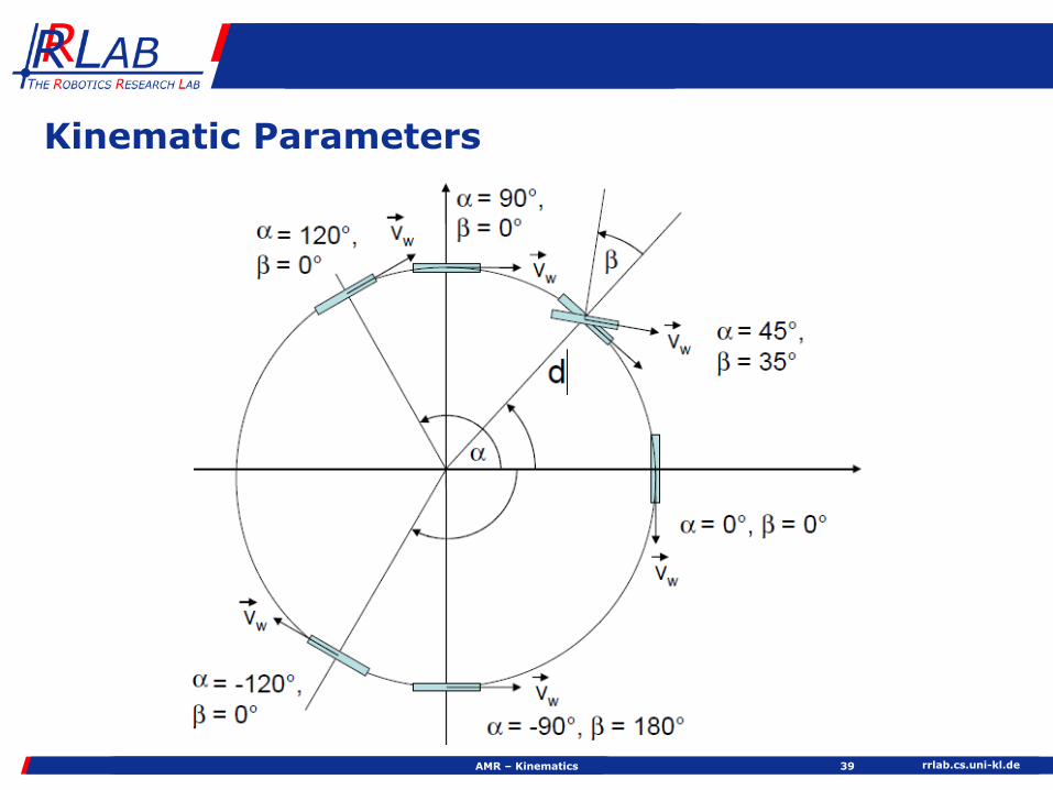
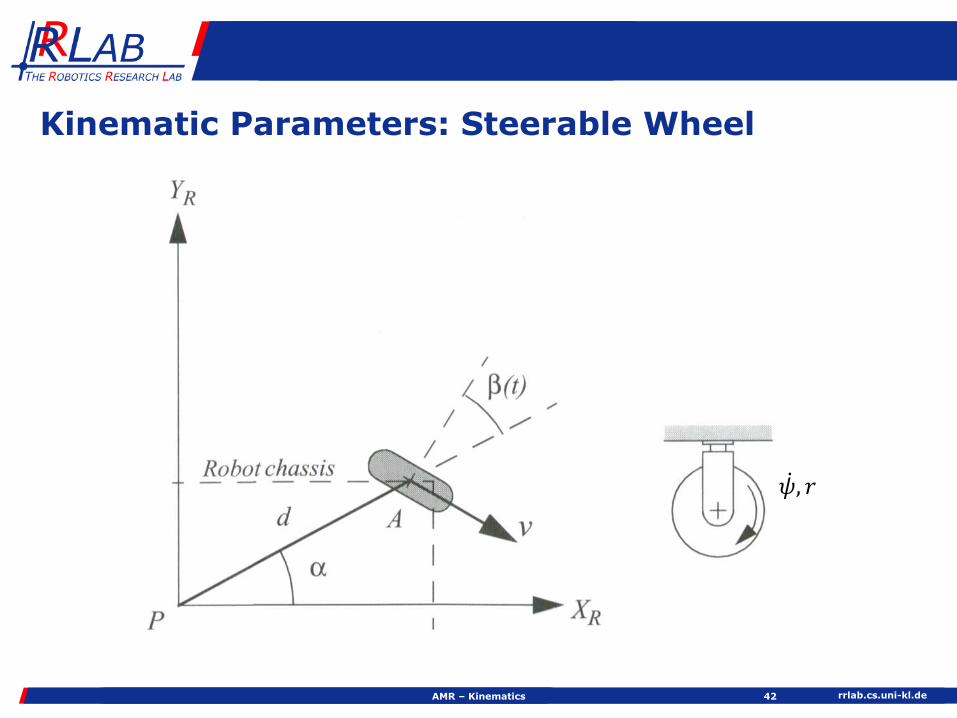
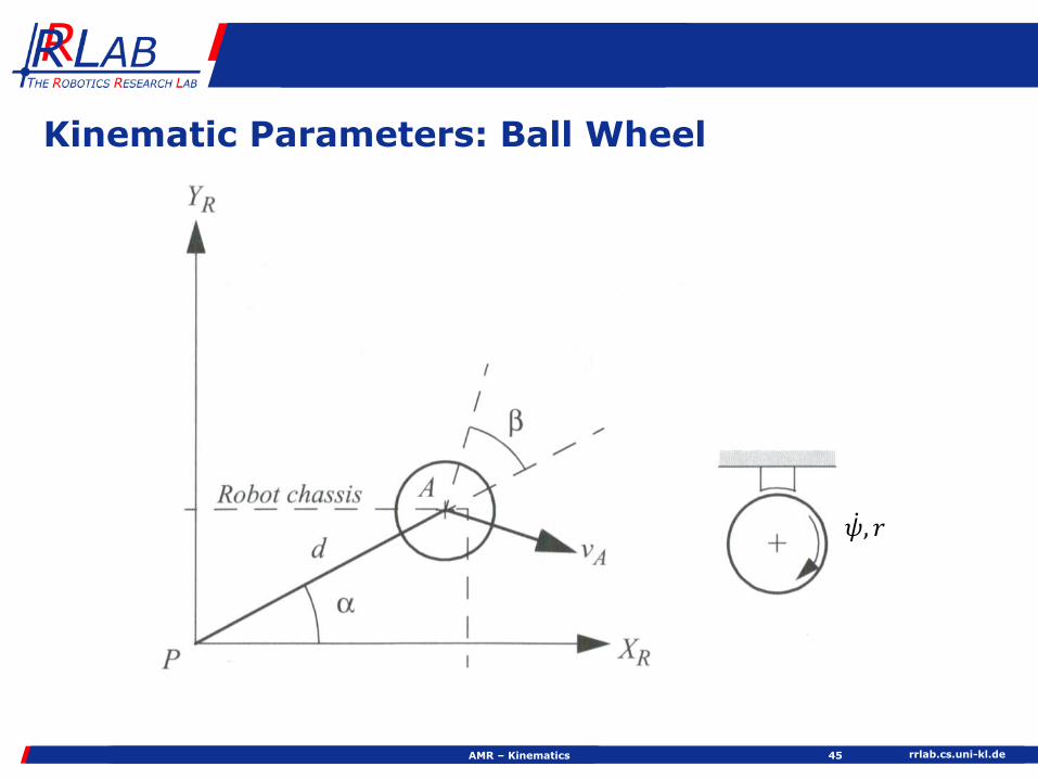
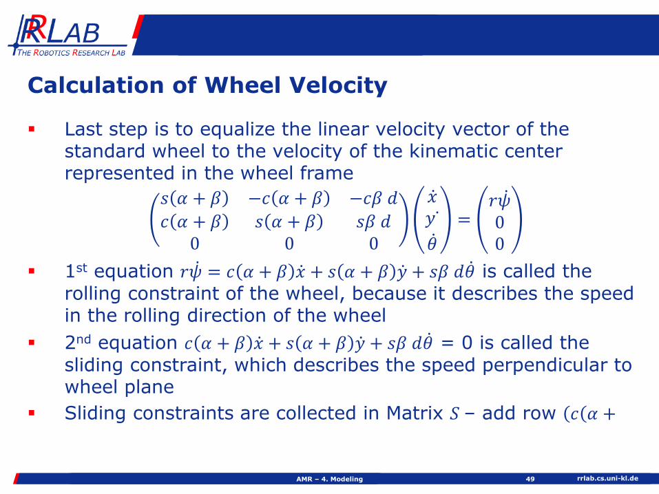
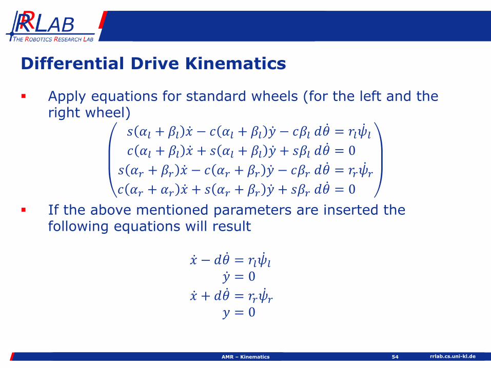
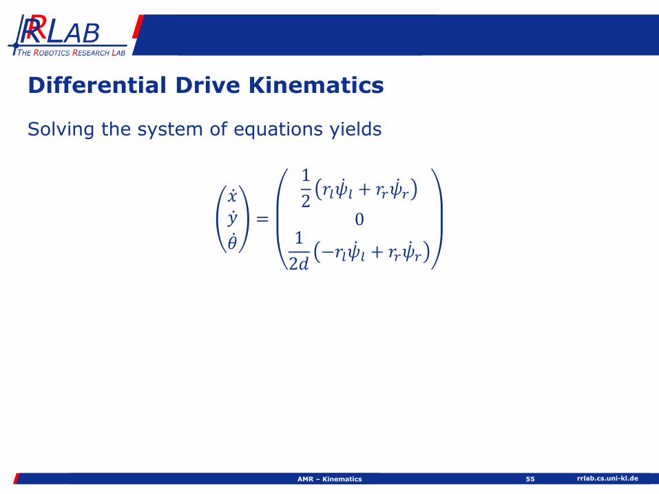

rrlabcsuni-klde
CROMSCI ndash Equipped with 3 Steerable Standard Wheels
AMR ndash Kinematics 57
Climbing robot CROMSCI Wheel settings of CROMSCI
rrlabcsuni-klde
Omnidirectional Drive Kinematics
AMR ndash Kinematics 58
Typical orientations of the 3 steerable wheels of an omnidirectional vehicle
rrlabcsuni-kldeAMR ndash Kinematicsg 59
Omnidirectional Drive Kinematics
Three steerable standard wheels
Kinematic center located in the middle of the robot
Distance between the kinematic center and each wheel 119889
Origin of coordinates frame is kinematic center
Kinematic parameters
1205721 = 0 deg
1205722 = 120 deg
1205723 = minus120 deg
rrlabcsuni-kldeAMR ndash Kinematics 60
Omnidirectional Drive Kinematics
Applying equation for steerable standard wheel for each wheel leads to the following system of equations
119904 1205721 + 1205731 ሶ119909 minus 119888 1205721 + 1205731 ሶ119910 minus 119889 sdot 119888 1205731 ሶ120579 = 1199031 ሶ1205951
119904 1205722 + 1205732 ሶ119909 minus 119888 1205722 + 1205732 ሶ119910 minus 119889 sdot 119888 1205732 ሶ120579 = 1199032 ሶ1205952
119904 1205723 + 1205733 ሶ119909 minus 119888 1205723 + 1205733 ሶ119910 minus 119889 sdot 119888 1205733 ሶ120579 = 1199033 ሶ1205953
119888 1205721 + 1205731 ሶ119909 + 119904 1205721 + 1205731 ሶ119910 + 119889 sdot 119904 1205731 ሶ120579 = 0
119888 1205722 + 1205732 ሶ119909 + 119904 1205722 + 1205732 ሶ119910 + 119889 sdot 119904 1205732 ሶ120579 = 0
119888 1205723 + 1205733 ሶ119909 + 119904 1205723 + 1205733 ሶ119910 + 119889 sdot 119904 1205733 ሶ120579 = 0
rrlabcsuni-kldeAMR ndash Kinematics 61
Omnidirectional Drive Kinematics
Based on these equation the steering angles 120573119894 119894 = 123 can be determined
119888 120572119894 + 120573119894 sdot ሶ119909 + 119904 120572119894 + 120573119894 sdot ሶ119910 + 119889 sdot 119904 120573119894 sdot ሶ120579 = 0
119888 120572119894 sdot 119888 120573119894 sdot ሶ119909 minus 119904 120572119894 sdot 119904 120573119894 sdot ሶ119909 + 119904 120572119894 sdot 119888 120573119894 sdot ሶ119910 + 119888 120572119894 sdot 119904 120573119894 sdot ሶ119910 + 119889 sdot 119904 120573119894 sdot ሶ120579 = 0
119888 120573119894 sdot 119888 120572119894 sdot ሶ119909 + 119904 120572119894 sdot ሶ119910 minus 119904 120573119894 sdot 119904 120572119894 sdot ሶ119909 minus 119888 120572119894 sdot ሶ119910 minus 119889 sdot ሶ120579 = 0
119888 120572119894 sdot ሶ119909 + 119904 120572119894 sdot ሶ119910
119904 120572119894 sdot ሶ119909 minus 119888 120572119894 sdot ሶ119910 minus 119889 sdot ሶ120579=119904 120573119894119888 120573119894
atan2 119888 120572119894 sdot ሶ119909 + 119904 120572119894 sdot ሶ119910 119904 120572119894 sdot ሶ119909 minus 119888 120572119894 sdot ሶ119910 minus 119889 sdot ሶ120579 = 120573119894
Also the angular velocity of the wheel ሶ120595119894 can now be calculated
ሶ120595119894 =1
119903119894119904 120572119894 + 120573119894 ሶ119909 minus 119888 120572119894 + 120573119894 ሶ119910 minus 119889 sdot 119888 120573119894 ሶ120579
rrlabcsuni-klde
The Climbing Robot CROMSCI
AMR ndash Kinematics 62
rrlabcsuni-klde
Mecanum Vehicle
AMR ndash Kinematics 63
Schematic configurationof a Mecanum wheel(Viewed from above)
The mobile robot PRIAMOS of the University of Karlsruhe driven by Mecanum wheels
rrlabcsuni-kldeAMR ndash Kinematics 64
Mecanum Kinematics
To set up the kinematic equation first the parameters 120572 120573 120574for each wheel must be determined
The parameters for four wheels are
1205721 = 45 deg 1205731 = 45 deg 1205741 = minus45 deg
1205722 = 135 deg 1205732 = minus45 deg 1205742 = 45 deg
1205723 = minus135 deg 1205733 = 225 deg 1205743 = minus45 deg
1205724 = minus45 deg 1205734 = 135 deg 1205744 = 45 deg
rrlabcsuni-kldeAMR ndash Kinematics 65
Mecanum Kinematics
Assume all driven wheels have the same radius 119903 the same distance 119889 from the kinematic center and the above mentioned parameters 120572 120573 120574
Using equation for Mecanum wheels leads to equations
119904 45 deg ሶ119909 minus 119888 45 deg ሶ119910 minus 119889 ሶ120579 = 119903 sdot 119888 minus45 deg ሶ1205951
119904 135 deg ሶ119909 minus 119888 135 deg ሶ119910 minus 119889 ሶ120579 = 119903 sdot 119888 45 deg ሶ1205952
119904 45 deg ሶ119909 minus 119888 45 deg ሶ119910 minus 119889 ሶ120579 = 119903 sdot 119888 minus45 deg ሶ1205953
119904 135 deg ሶ119909 minus 119888 135 deg ሶ119910 minus 119889 ሶ120579 = 119903 sdot 119888 45 deg ሶ1205954
rrlabcsuni-kldeAMR ndash Kinematics 66
Mecanum Kinematics
The velocities ሶ119909 ሶ119910 ሶ120579 of the kinematic center can be calculated
ሶ119909 =119903
4ሶ1205951 + ሶ1205952 + ሶ1205953 + ሶ1205954
ሶ119910 =119903
4minus ሶ1205951 + ሶ1205952 minus ሶ1205953 + ሶ1205954
ሶ120579 =119903
119889 2ሶ1205951 minus ሶ1205952 minus ሶ1205953 + ሶ1205954
rrlabcsuni-kldeAMR ndash Kinematics 67
Mecanum Kinematics
The velocity vector of the kinematic center can be determined as
ሶ119909ሶ119910ሶ120579
=119903119908ℎ1198901198901198974
sdot1 1 1 1minus1 1 minus1 1119886 minus119886 minus119886 119886
sdot
ሶ1205951
ሶ1205952
ሶ1205953
ሶ1205954
with a =2 2
119889
Assuming the absence of slip the following must hold
ሶ1205954 = ሶ1205951 + ሶ1205952 minus ሶ1205953
rrlabcsuni-klde
Maneuverability of AMRs
rrlabcsuni-kldeAMR ndash Maneuverability 69
Choice of Wheel Configuration
Choice of wheels and their configuration depends on hellip
Ability to maneuver
Controllability
Stability
An optimum can only be achieved concerning a specific application
rrlabcsuni-kldeAMR ndash Maneuverability 70
Stability
Minimal number of wheels for static stability is 2 if center of gravity is located under the wheel axis (e g robot Cye)
Under standard conditions itrsquos 3
If more than 3 wheels are present adjustment to rough terrain becomes necessary
Typical setups
2 driven wheels on a single axis with 1 or 2 passive castor wheels
Single driven and steered wheel with two passive fixed wheels
rrlabcsuni-kldeAMR ndash Maneuverability 71
Maneuverability
Robotrsquos degree of freedom (DOF)
Outstanding ability to maneuver when the only driven wheel can be rotated in an active way
Example Ackermann steering
Poor ability to maneuver
5 m radius required for single rotation of a car
Lateral movement only possible troughforwardbackward movement
rrlabcsuni-kldeAMR ndash Maneuverability 72
Controllability
Costs for locomotion of the robot on a given trajectory
Contradiction to the robotrsquos ability to maneuver
Examples
Ackermann steering easy to control
Mecanum wheels very costly if high precision is required
Costs for controllability depend on hellip
Wheel type
Drive geometry
Sensors to determine driving situation
Motortransmission
rrlabcsuni-kldeAMR ndash Maneuverability 73
Degree of Mobility
The degree of mobility 119891119898 isin 123 points out how the sliding constraints (defined in Matrix 119878 see slide 42) affect the
possibilities for robot movement 119877 120579 ሶ120585119897 The mobility can be calculated by using the rank of the
matrix of sliding constraints of all standard wheels (steerable and fixed wheels) = number of independent constraints
119891119898 = 3 minus rank 119878
rrlabcsuni-kldeAMR ndash Maneuverability 74
Degree of Mobility
Example Differential Drive
Given only two fixed wheels geometrically we can set
1198891 = 1198892 1205731 = 1205732 = 0 1205721 + 120587 = 1205722
Matrix 119878 has two sliding constraints of the form (119888(120572 +
rrlabcsuni-kldeAMR ndash Maneuverability 75
Degree of Steerability
The degree of steerability 119891119904 isin 012 quantifies the degree of controllable freedom and is determined via the number of independently controllable steering parameters
Define 119878prime Part of 119878 defining sliding constraints of steerable wheels
119891119904 = rank 119878prime
More possibilities in steering will result in lower mobility
119891119904 = 0 No steered wheel (differential drive)
119891119904 = 1 At least one steered wheel (Ackermann steering)
119891119904 = 2 At least two steered wheels no fixed wheel
rrlabcsuni-kldeAMR ndash Maneuverability 76
Degree of Maneuverability
The degree of maneuverability 119891119872 isin 23 points out the number of DOF the robot can manipulate
119891119872 = 119891119898 + 119891119904
rrlabcsuni-klde
Vehicle Kinematics
Geometrical Solution
rrlabcsuni-kldeAMR ndash Kinematics 78
Tricycle Drive
Given 120575 119907
Unknown 119907prime 119907119897 119907119903 Solution
119903 = 119897 sdot cot 120575
119907prime =119907
cos 120575
119907119897 = 119907 sdot119903 + 119889
119903
119907119903 = 119907 sdot119903 minus 119889
119903 Tricycle drive kinematics
120575
rrlabcsuni-kldeAMR ndash 4 Kinematics 79
Ackermann Steering
Given 119907119863 120575 119897 119889
Unknown 119907119903119903 119907119897119903 119907119903119891 119907119897119891
Solution
120602 =119897
tan 120575
119907119897119903 =120602 minus 1198892 sdot 119907119863
120602
119907119903119903 =120602 + 1198892 sdot 119907119863
120602
119907119897119891 =120602 minus 1198892 2 + 1198972 sdot tan 120575
119897sdot 119907119863
119907119903119891 =1206022 + 1198972 sdot tan 120575
119897sdot 119907119863
Kinematics ofAckermann steering
120575
120602
rrlabcsuni-klde
Omnidrive Kinematics
AMR ndash Kinematics 80
Given 120602 120593 119907 119889
Unknown 1205931 1205932 1199071 1199072 Solution
120549119909 = 120602 sdot cos120593120549119910 = 120602 sdot sin1205931205931 = arctan120549119910 minus 1198891205491199091206021 = 120602 sdot cos120593 cos12059311199071 = 119907 sdot 1206021120602
1205932 = arctan120549119910 + 119889
1205491199091206022 = 120602 sdot cos120593 cos1205932
1199072 = 119907 sdot 1206022120602
120549119910 = 120602 ∙ 119904119894119899 120593
1205931
1205932
1206021
1206022
120593 120549119909 = 120602 ∙ cos120593
120602
119889
rrlabcsuni-klde
Bicycle Model
AMR ndash Kinematics 81
119907
rrlabcsuni-kldeAMR ndash Kinematics 82
Bicycle Model
Circular road of radius 120602
Low speed motion
Slip angles at both wheels are zero
Small total lateral force from both tires
119865119910 =1198981199072
120602
Point 119875 is instantaneous rolling center
Velocity at 119862 is perpendicular to line 119875119862
Heading angle 120579
Slip angle 120575119907 Course angle 120574 = 120579 + 120575119907
rrlabcsuni-kldeAMR ndash 4 Modeling 83
Bicycle Model
Given 120575119891 120575119903 119907 120579
Unknown ሶ119883 ሶ119884 ሶ120579
Solution
120575119907 = tanminus1119897119891 tan 120575119903+119897119903 tan 120575119891
119897119891+119897119903
ሶ120579 =119907
120602
120602 =119897119891+119897119903
tan 120575119891 minustan 120575119903 cos 120575119907
ሶ119883 = 119907 cos 120579 + 120575119907ሶ119884 = 119907 sin 120579 + 120575119907
ሶ120579 =119907 cos 120575119907
119897119891+119897119903tan 120575119891 minus tan 120575119903
119907
rrlabcsuni-klde
Ackermann Steering -gt Bicycle Model
AMR ndash Kinematics 84
119862 = 119874 120575119903 = 0 120575119891 = 120575
119897119903 = 0 119897119891 = 119897
120575119907 = 0
ሶ120579 =119907
120602
120602 =119897
tan 120575119891
ሶ119883 = 119907 cos 120579ሶ119884 = 119907 sin 120579ሶ120579 =
119907
119897119891tan 120575119891
119907
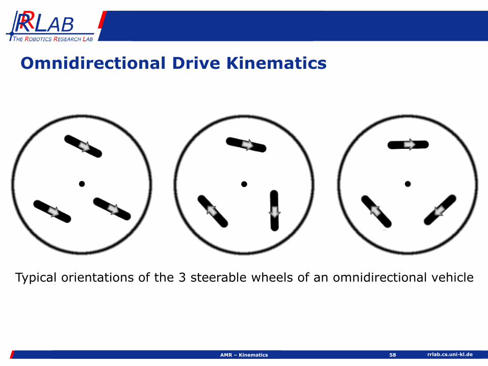
rrlabcsuni-klde
Omnidirectional Drive Kinematics
AMR ndash Kinematics 58
Typical orientations of the 3 steerable wheels of an omnidirectional vehicle
rrlabcsuni-kldeAMR ndash Kinematicsg 59
Omnidirectional Drive Kinematics
Three steerable standard wheels
Kinematic center located in the middle of the robot
Distance between the kinematic center and each wheel 119889
Origin of coordinates frame is kinematic center
Kinematic parameters
1205721 = 0 deg
1205722 = 120 deg
1205723 = minus120 deg
rrlabcsuni-kldeAMR ndash Kinematics 60
Omnidirectional Drive Kinematics
Applying equation for steerable standard wheel for each wheel leads to the following system of equations
119904 1205721 + 1205731 ሶ119909 minus 119888 1205721 + 1205731 ሶ119910 minus 119889 sdot 119888 1205731 ሶ120579 = 1199031 ሶ1205951
119904 1205722 + 1205732 ሶ119909 minus 119888 1205722 + 1205732 ሶ119910 minus 119889 sdot 119888 1205732 ሶ120579 = 1199032 ሶ1205952
119904 1205723 + 1205733 ሶ119909 minus 119888 1205723 + 1205733 ሶ119910 minus 119889 sdot 119888 1205733 ሶ120579 = 1199033 ሶ1205953
119888 1205721 + 1205731 ሶ119909 + 119904 1205721 + 1205731 ሶ119910 + 119889 sdot 119904 1205731 ሶ120579 = 0
119888 1205722 + 1205732 ሶ119909 + 119904 1205722 + 1205732 ሶ119910 + 119889 sdot 119904 1205732 ሶ120579 = 0
119888 1205723 + 1205733 ሶ119909 + 119904 1205723 + 1205733 ሶ119910 + 119889 sdot 119904 1205733 ሶ120579 = 0
rrlabcsuni-kldeAMR ndash Kinematics 61
Omnidirectional Drive Kinematics
Based on these equation the steering angles 120573119894 119894 = 123 can be determined
119888 120572119894 + 120573119894 sdot ሶ119909 + 119904 120572119894 + 120573119894 sdot ሶ119910 + 119889 sdot 119904 120573119894 sdot ሶ120579 = 0
119888 120572119894 sdot 119888 120573119894 sdot ሶ119909 minus 119904 120572119894 sdot 119904 120573119894 sdot ሶ119909 + 119904 120572119894 sdot 119888 120573119894 sdot ሶ119910 + 119888 120572119894 sdot 119904 120573119894 sdot ሶ119910 + 119889 sdot 119904 120573119894 sdot ሶ120579 = 0
119888 120573119894 sdot 119888 120572119894 sdot ሶ119909 + 119904 120572119894 sdot ሶ119910 minus 119904 120573119894 sdot 119904 120572119894 sdot ሶ119909 minus 119888 120572119894 sdot ሶ119910 minus 119889 sdot ሶ120579 = 0
119888 120572119894 sdot ሶ119909 + 119904 120572119894 sdot ሶ119910
119904 120572119894 sdot ሶ119909 minus 119888 120572119894 sdot ሶ119910 minus 119889 sdot ሶ120579=119904 120573119894119888 120573119894
atan2 119888 120572119894 sdot ሶ119909 + 119904 120572119894 sdot ሶ119910 119904 120572119894 sdot ሶ119909 minus 119888 120572119894 sdot ሶ119910 minus 119889 sdot ሶ120579 = 120573119894
Also the angular velocity of the wheel ሶ120595119894 can now be calculated
ሶ120595119894 =1
119903119894119904 120572119894 + 120573119894 ሶ119909 minus 119888 120572119894 + 120573119894 ሶ119910 minus 119889 sdot 119888 120573119894 ሶ120579
rrlabcsuni-klde
The Climbing Robot CROMSCI
AMR ndash Kinematics 62
rrlabcsuni-klde
Mecanum Vehicle
AMR ndash Kinematics 63
Schematic configurationof a Mecanum wheel(Viewed from above)
The mobile robot PRIAMOS of the University of Karlsruhe driven by Mecanum wheels
rrlabcsuni-kldeAMR ndash Kinematics 64
Mecanum Kinematics
To set up the kinematic equation first the parameters 120572 120573 120574for each wheel must be determined
The parameters for four wheels are
1205721 = 45 deg 1205731 = 45 deg 1205741 = minus45 deg
1205722 = 135 deg 1205732 = minus45 deg 1205742 = 45 deg
1205723 = minus135 deg 1205733 = 225 deg 1205743 = minus45 deg
1205724 = minus45 deg 1205734 = 135 deg 1205744 = 45 deg
rrlabcsuni-kldeAMR ndash Kinematics 65
Mecanum Kinematics
Assume all driven wheels have the same radius 119903 the same distance 119889 from the kinematic center and the above mentioned parameters 120572 120573 120574
Using equation for Mecanum wheels leads to equations
119904 45 deg ሶ119909 minus 119888 45 deg ሶ119910 minus 119889 ሶ120579 = 119903 sdot 119888 minus45 deg ሶ1205951
119904 135 deg ሶ119909 minus 119888 135 deg ሶ119910 minus 119889 ሶ120579 = 119903 sdot 119888 45 deg ሶ1205952
119904 45 deg ሶ119909 minus 119888 45 deg ሶ119910 minus 119889 ሶ120579 = 119903 sdot 119888 minus45 deg ሶ1205953
119904 135 deg ሶ119909 minus 119888 135 deg ሶ119910 minus 119889 ሶ120579 = 119903 sdot 119888 45 deg ሶ1205954
rrlabcsuni-kldeAMR ndash Kinematics 66
Mecanum Kinematics
The velocities ሶ119909 ሶ119910 ሶ120579 of the kinematic center can be calculated
ሶ119909 =119903
4ሶ1205951 + ሶ1205952 + ሶ1205953 + ሶ1205954
ሶ119910 =119903
4minus ሶ1205951 + ሶ1205952 minus ሶ1205953 + ሶ1205954
ሶ120579 =119903
119889 2ሶ1205951 minus ሶ1205952 minus ሶ1205953 + ሶ1205954
rrlabcsuni-kldeAMR ndash Kinematics 67
Mecanum Kinematics
The velocity vector of the kinematic center can be determined as
ሶ119909ሶ119910ሶ120579
=119903119908ℎ1198901198901198974
sdot1 1 1 1minus1 1 minus1 1119886 minus119886 minus119886 119886
sdot
ሶ1205951
ሶ1205952
ሶ1205953
ሶ1205954
with a =2 2
119889
Assuming the absence of slip the following must hold
ሶ1205954 = ሶ1205951 + ሶ1205952 minus ሶ1205953
rrlabcsuni-klde
Maneuverability of AMRs
rrlabcsuni-kldeAMR ndash Maneuverability 69
Choice of Wheel Configuration
Choice of wheels and their configuration depends on hellip
Ability to maneuver
Controllability
Stability
An optimum can only be achieved concerning a specific application
rrlabcsuni-kldeAMR ndash Maneuverability 70
Stability
Minimal number of wheels for static stability is 2 if center of gravity is located under the wheel axis (e g robot Cye)
Under standard conditions itrsquos 3
If more than 3 wheels are present adjustment to rough terrain becomes necessary
Typical setups
2 driven wheels on a single axis with 1 or 2 passive castor wheels
Single driven and steered wheel with two passive fixed wheels
rrlabcsuni-kldeAMR ndash Maneuverability 71
Maneuverability
Robotrsquos degree of freedom (DOF)
Outstanding ability to maneuver when the only driven wheel can be rotated in an active way
Example Ackermann steering
Poor ability to maneuver
5 m radius required for single rotation of a car
Lateral movement only possible troughforwardbackward movement
rrlabcsuni-kldeAMR ndash Maneuverability 72
Controllability
Costs for locomotion of the robot on a given trajectory
Contradiction to the robotrsquos ability to maneuver
Examples
Ackermann steering easy to control
Mecanum wheels very costly if high precision is required
Costs for controllability depend on hellip
Wheel type
Drive geometry
Sensors to determine driving situation
Motortransmission
rrlabcsuni-kldeAMR ndash Maneuverability 73
Degree of Mobility
The degree of mobility 119891119898 isin 123 points out how the sliding constraints (defined in Matrix 119878 see slide 42) affect the
possibilities for robot movement 119877 120579 ሶ120585119897 The mobility can be calculated by using the rank of the
matrix of sliding constraints of all standard wheels (steerable and fixed wheels) = number of independent constraints
119891119898 = 3 minus rank 119878
rrlabcsuni-kldeAMR ndash Maneuverability 74
Degree of Mobility
Example Differential Drive
Given only two fixed wheels geometrically we can set
1198891 = 1198892 1205731 = 1205732 = 0 1205721 + 120587 = 1205722
Matrix 119878 has two sliding constraints of the form (119888(120572 +
rrlabcsuni-kldeAMR ndash Maneuverability 75
Degree of Steerability
The degree of steerability 119891119904 isin 012 quantifies the degree of controllable freedom and is determined via the number of independently controllable steering parameters
Define 119878prime Part of 119878 defining sliding constraints of steerable wheels
119891119904 = rank 119878prime
More possibilities in steering will result in lower mobility
119891119904 = 0 No steered wheel (differential drive)
119891119904 = 1 At least one steered wheel (Ackermann steering)
119891119904 = 2 At least two steered wheels no fixed wheel
rrlabcsuni-kldeAMR ndash Maneuverability 76
Degree of Maneuverability
The degree of maneuverability 119891119872 isin 23 points out the number of DOF the robot can manipulate
119891119872 = 119891119898 + 119891119904
rrlabcsuni-klde
Vehicle Kinematics
Geometrical Solution
rrlabcsuni-kldeAMR ndash Kinematics 78
Tricycle Drive
Given 120575 119907
Unknown 119907prime 119907119897 119907119903 Solution
119903 = 119897 sdot cot 120575
119907prime =119907
cos 120575
119907119897 = 119907 sdot119903 + 119889
119903
119907119903 = 119907 sdot119903 minus 119889
119903 Tricycle drive kinematics
120575
rrlabcsuni-kldeAMR ndash 4 Kinematics 79
Ackermann Steering
Given 119907119863 120575 119897 119889
Unknown 119907119903119903 119907119897119903 119907119903119891 119907119897119891
Solution
120602 =119897
tan 120575
119907119897119903 =120602 minus 1198892 sdot 119907119863
120602
119907119903119903 =120602 + 1198892 sdot 119907119863
120602
119907119897119891 =120602 minus 1198892 2 + 1198972 sdot tan 120575
119897sdot 119907119863
119907119903119891 =1206022 + 1198972 sdot tan 120575
119897sdot 119907119863
Kinematics ofAckermann steering
120575
120602
rrlabcsuni-klde
Omnidrive Kinematics
AMR ndash Kinematics 80
Given 120602 120593 119907 119889
Unknown 1205931 1205932 1199071 1199072 Solution
120549119909 = 120602 sdot cos120593120549119910 = 120602 sdot sin1205931205931 = arctan120549119910 minus 1198891205491199091206021 = 120602 sdot cos120593 cos12059311199071 = 119907 sdot 1206021120602
1205932 = arctan120549119910 + 119889
1205491199091206022 = 120602 sdot cos120593 cos1205932
1199072 = 119907 sdot 1206022120602
120549119910 = 120602 ∙ 119904119894119899 120593
1205931
1205932
1206021
1206022
120593 120549119909 = 120602 ∙ cos120593
120602
119889
rrlabcsuni-klde
Bicycle Model
AMR ndash Kinematics 81
119907
rrlabcsuni-kldeAMR ndash Kinematics 82
Bicycle Model
Circular road of radius 120602
Low speed motion
Slip angles at both wheels are zero
Small total lateral force from both tires
119865119910 =1198981199072
120602
Point 119875 is instantaneous rolling center
Velocity at 119862 is perpendicular to line 119875119862
Heading angle 120579
Slip angle 120575119907 Course angle 120574 = 120579 + 120575119907
rrlabcsuni-kldeAMR ndash 4 Modeling 83
Bicycle Model
Given 120575119891 120575119903 119907 120579
Unknown ሶ119883 ሶ119884 ሶ120579
Solution
120575119907 = tanminus1119897119891 tan 120575119903+119897119903 tan 120575119891
119897119891+119897119903
ሶ120579 =119907
120602
120602 =119897119891+119897119903
tan 120575119891 minustan 120575119903 cos 120575119907
ሶ119883 = 119907 cos 120579 + 120575119907ሶ119884 = 119907 sin 120579 + 120575119907
ሶ120579 =119907 cos 120575119907
119897119891+119897119903tan 120575119891 minus tan 120575119903
119907
rrlabcsuni-klde
Ackermann Steering -gt Bicycle Model
AMR ndash Kinematics 84
119862 = 119874 120575119903 = 0 120575119891 = 120575
119897119903 = 0 119897119891 = 119897
120575119907 = 0
ሶ120579 =119907
120602
120602 =119897
tan 120575119891
ሶ119883 = 119907 cos 120579ሶ119884 = 119907 sin 120579ሶ120579 =
119907
119897119891tan 120575119891
119907
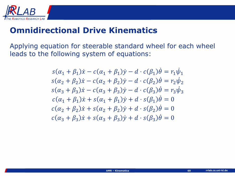

rrlabcsuni-klde
Mecanum Vehicle
AMR ndash Kinematics 63
Schematic configurationof a Mecanum wheel(Viewed from above)
The mobile robot PRIAMOS of the University of Karlsruhe driven by Mecanum wheels
rrlabcsuni-kldeAMR ndash Kinematics 64
Mecanum Kinematics
To set up the kinematic equation first the parameters 120572 120573 120574for each wheel must be determined
The parameters for four wheels are
1205721 = 45 deg 1205731 = 45 deg 1205741 = minus45 deg
1205722 = 135 deg 1205732 = minus45 deg 1205742 = 45 deg
1205723 = minus135 deg 1205733 = 225 deg 1205743 = minus45 deg
1205724 = minus45 deg 1205734 = 135 deg 1205744 = 45 deg
rrlabcsuni-kldeAMR ndash Kinematics 65
Mecanum Kinematics
Assume all driven wheels have the same radius 119903 the same distance 119889 from the kinematic center and the above mentioned parameters 120572 120573 120574
Using equation for Mecanum wheels leads to equations
119904 45 deg ሶ119909 minus 119888 45 deg ሶ119910 minus 119889 ሶ120579 = 119903 sdot 119888 minus45 deg ሶ1205951
119904 135 deg ሶ119909 minus 119888 135 deg ሶ119910 minus 119889 ሶ120579 = 119903 sdot 119888 45 deg ሶ1205952
119904 45 deg ሶ119909 minus 119888 45 deg ሶ119910 minus 119889 ሶ120579 = 119903 sdot 119888 minus45 deg ሶ1205953
119904 135 deg ሶ119909 minus 119888 135 deg ሶ119910 minus 119889 ሶ120579 = 119903 sdot 119888 45 deg ሶ1205954
rrlabcsuni-kldeAMR ndash Kinematics 66
Mecanum Kinematics
The velocities ሶ119909 ሶ119910 ሶ120579 of the kinematic center can be calculated
ሶ119909 =119903
4ሶ1205951 + ሶ1205952 + ሶ1205953 + ሶ1205954
ሶ119910 =119903
4minus ሶ1205951 + ሶ1205952 minus ሶ1205953 + ሶ1205954
ሶ120579 =119903
119889 2ሶ1205951 minus ሶ1205952 minus ሶ1205953 + ሶ1205954
rrlabcsuni-kldeAMR ndash Kinematics 67
Mecanum Kinematics
The velocity vector of the kinematic center can be determined as
ሶ119909ሶ119910ሶ120579
=119903119908ℎ1198901198901198974
sdot1 1 1 1minus1 1 minus1 1119886 minus119886 minus119886 119886
sdot
ሶ1205951
ሶ1205952
ሶ1205953
ሶ1205954
with a =2 2
119889
Assuming the absence of slip the following must hold
ሶ1205954 = ሶ1205951 + ሶ1205952 minus ሶ1205953
rrlabcsuni-klde
Maneuverability of AMRs
rrlabcsuni-kldeAMR ndash Maneuverability 69
Choice of Wheel Configuration
Choice of wheels and their configuration depends on hellip
Ability to maneuver
Controllability
Stability
An optimum can only be achieved concerning a specific application
rrlabcsuni-kldeAMR ndash Maneuverability 70
Stability
Minimal number of wheels for static stability is 2 if center of gravity is located under the wheel axis (e g robot Cye)
Under standard conditions itrsquos 3
If more than 3 wheels are present adjustment to rough terrain becomes necessary
Typical setups
2 driven wheels on a single axis with 1 or 2 passive castor wheels
Single driven and steered wheel with two passive fixed wheels
rrlabcsuni-kldeAMR ndash Maneuverability 71
Maneuverability
Robotrsquos degree of freedom (DOF)
Outstanding ability to maneuver when the only driven wheel can be rotated in an active way
Example Ackermann steering
Poor ability to maneuver
5 m radius required for single rotation of a car
Lateral movement only possible troughforwardbackward movement
rrlabcsuni-kldeAMR ndash Maneuverability 72
Controllability
Costs for locomotion of the robot on a given trajectory
Contradiction to the robotrsquos ability to maneuver
Examples
Ackermann steering easy to control
Mecanum wheels very costly if high precision is required
Costs for controllability depend on hellip
Wheel type
Drive geometry
Sensors to determine driving situation
Motortransmission
rrlabcsuni-kldeAMR ndash Maneuverability 73
Degree of Mobility
The degree of mobility 119891119898 isin 123 points out how the sliding constraints (defined in Matrix 119878 see slide 42) affect the
possibilities for robot movement 119877 120579 ሶ120585119897 The mobility can be calculated by using the rank of the
matrix of sliding constraints of all standard wheels (steerable and fixed wheels) = number of independent constraints
119891119898 = 3 minus rank 119878
rrlabcsuni-kldeAMR ndash Maneuverability 74
Degree of Mobility
Example Differential Drive
Given only two fixed wheels geometrically we can set
1198891 = 1198892 1205731 = 1205732 = 0 1205721 + 120587 = 1205722
Matrix 119878 has two sliding constraints of the form (119888(120572 +
rrlabcsuni-kldeAMR ndash Maneuverability 75
Degree of Steerability
The degree of steerability 119891119904 isin 012 quantifies the degree of controllable freedom and is determined via the number of independently controllable steering parameters
Define 119878prime Part of 119878 defining sliding constraints of steerable wheels
119891119904 = rank 119878prime
More possibilities in steering will result in lower mobility
119891119904 = 0 No steered wheel (differential drive)
119891119904 = 1 At least one steered wheel (Ackermann steering)
119891119904 = 2 At least two steered wheels no fixed wheel
rrlabcsuni-kldeAMR ndash Maneuverability 76
Degree of Maneuverability
The degree of maneuverability 119891119872 isin 23 points out the number of DOF the robot can manipulate
119891119872 = 119891119898 + 119891119904
rrlabcsuni-klde
Vehicle Kinematics
Geometrical Solution
rrlabcsuni-kldeAMR ndash Kinematics 78
Tricycle Drive
Given 120575 119907
Unknown 119907prime 119907119897 119907119903 Solution
119903 = 119897 sdot cot 120575
119907prime =119907
cos 120575
119907119897 = 119907 sdot119903 + 119889
119903
119907119903 = 119907 sdot119903 minus 119889
119903 Tricycle drive kinematics
120575
rrlabcsuni-kldeAMR ndash 4 Kinematics 79
Ackermann Steering
Given 119907119863 120575 119897 119889
Unknown 119907119903119903 119907119897119903 119907119903119891 119907119897119891
Solution
120602 =119897
tan 120575
119907119897119903 =120602 minus 1198892 sdot 119907119863
120602
119907119903119903 =120602 + 1198892 sdot 119907119863
120602
119907119897119891 =120602 minus 1198892 2 + 1198972 sdot tan 120575
119897sdot 119907119863
119907119903119891 =1206022 + 1198972 sdot tan 120575
119897sdot 119907119863
Kinematics ofAckermann steering
120575
120602
rrlabcsuni-klde
Omnidrive Kinematics
AMR ndash Kinematics 80
Given 120602 120593 119907 119889
Unknown 1205931 1205932 1199071 1199072 Solution
120549119909 = 120602 sdot cos120593120549119910 = 120602 sdot sin1205931205931 = arctan120549119910 minus 1198891205491199091206021 = 120602 sdot cos120593 cos12059311199071 = 119907 sdot 1206021120602
1205932 = arctan120549119910 + 119889
1205491199091206022 = 120602 sdot cos120593 cos1205932
1199072 = 119907 sdot 1206022120602
120549119910 = 120602 ∙ 119904119894119899 120593
1205931
1205932
1206021
1206022
120593 120549119909 = 120602 ∙ cos120593
120602
119889
rrlabcsuni-klde
Bicycle Model
AMR ndash Kinematics 81
119907
rrlabcsuni-kldeAMR ndash Kinematics 82
Bicycle Model
Circular road of radius 120602
Low speed motion
Slip angles at both wheels are zero
Small total lateral force from both tires
119865119910 =1198981199072
120602
Point 119875 is instantaneous rolling center
Velocity at 119862 is perpendicular to line 119875119862
Heading angle 120579
Slip angle 120575119907 Course angle 120574 = 120579 + 120575119907
rrlabcsuni-kldeAMR ndash 4 Modeling 83
Bicycle Model
Given 120575119891 120575119903 119907 120579
Unknown ሶ119883 ሶ119884 ሶ120579
Solution
120575119907 = tanminus1119897119891 tan 120575119903+119897119903 tan 120575119891
119897119891+119897119903
ሶ120579 =119907
120602
120602 =119897119891+119897119903
tan 120575119891 minustan 120575119903 cos 120575119907
ሶ119883 = 119907 cos 120579 + 120575119907ሶ119884 = 119907 sin 120579 + 120575119907
ሶ120579 =119907 cos 120575119907
119897119891+119897119903tan 120575119891 minus tan 120575119903
119907
rrlabcsuni-klde
Ackermann Steering -gt Bicycle Model
AMR ndash Kinematics 84
119862 = 119874 120575119903 = 0 120575119891 = 120575
119897119903 = 0 119897119891 = 119897
120575119907 = 0
ሶ120579 =119907
120602
120602 =119897
tan 120575119891
ሶ119883 = 119907 cos 120579ሶ119884 = 119907 sin 120579ሶ120579 =
119907
119897119891tan 120575119891
119907
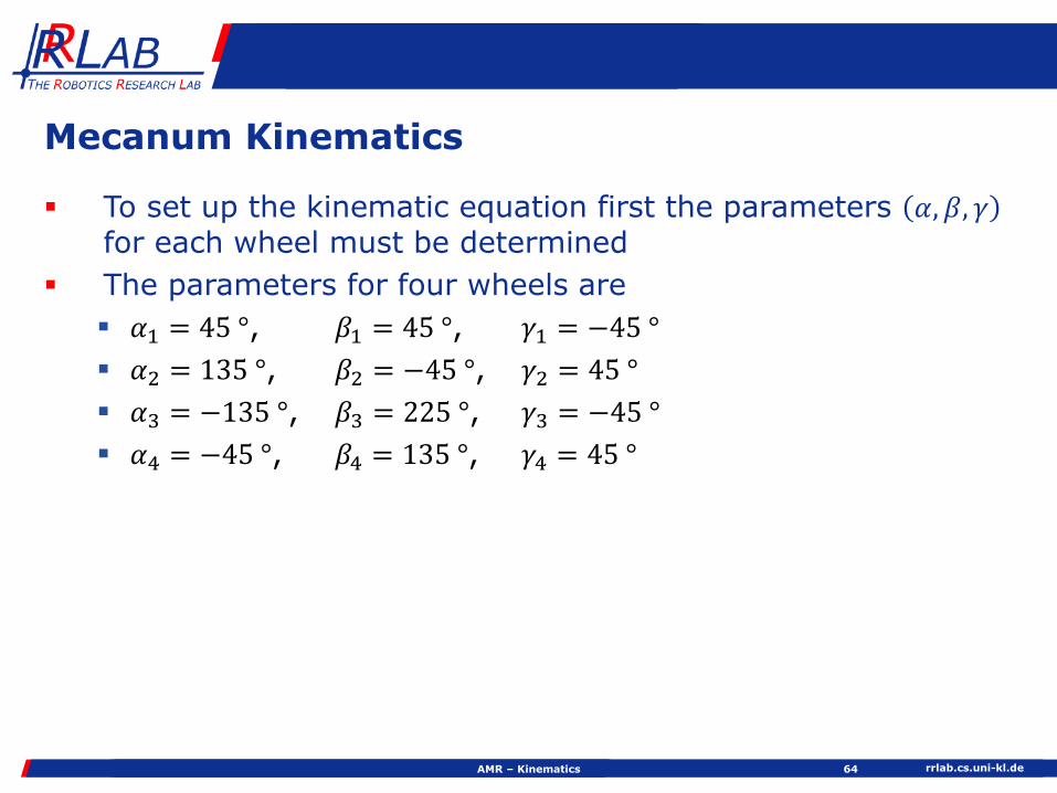

rrlabcsuni-klde
Maneuverability of AMRs
rrlabcsuni-kldeAMR ndash Maneuverability 69
Choice of Wheel Configuration
Choice of wheels and their configuration depends on hellip
Ability to maneuver
Controllability
Stability
An optimum can only be achieved concerning a specific application
rrlabcsuni-kldeAMR ndash Maneuverability 70
Stability
Minimal number of wheels for static stability is 2 if center of gravity is located under the wheel axis (e g robot Cye)
Under standard conditions itrsquos 3
If more than 3 wheels are present adjustment to rough terrain becomes necessary
Typical setups
2 driven wheels on a single axis with 1 or 2 passive castor wheels
Single driven and steered wheel with two passive fixed wheels
rrlabcsuni-kldeAMR ndash Maneuverability 71
Maneuverability
Robotrsquos degree of freedom (DOF)
Outstanding ability to maneuver when the only driven wheel can be rotated in an active way
Example Ackermann steering
Poor ability to maneuver
5 m radius required for single rotation of a car
Lateral movement only possible troughforwardbackward movement
rrlabcsuni-kldeAMR ndash Maneuverability 72
Controllability
Costs for locomotion of the robot on a given trajectory
Contradiction to the robotrsquos ability to maneuver
Examples
Ackermann steering easy to control
Mecanum wheels very costly if high precision is required
Costs for controllability depend on hellip
Wheel type
Drive geometry
Sensors to determine driving situation
Motortransmission
rrlabcsuni-kldeAMR ndash Maneuverability 73
Degree of Mobility
The degree of mobility 119891119898 isin 123 points out how the sliding constraints (defined in Matrix 119878 see slide 42) affect the
possibilities for robot movement 119877 120579 ሶ120585119897 The mobility can be calculated by using the rank of the
matrix of sliding constraints of all standard wheels (steerable and fixed wheels) = number of independent constraints
119891119898 = 3 minus rank 119878
rrlabcsuni-kldeAMR ndash Maneuverability 74
Degree of Mobility
Example Differential Drive
Given only two fixed wheels geometrically we can set
1198891 = 1198892 1205731 = 1205732 = 0 1205721 + 120587 = 1205722
Matrix 119878 has two sliding constraints of the form (119888(120572 +
rrlabcsuni-kldeAMR ndash Maneuverability 75
Degree of Steerability
The degree of steerability 119891119904 isin 012 quantifies the degree of controllable freedom and is determined via the number of independently controllable steering parameters
Define 119878prime Part of 119878 defining sliding constraints of steerable wheels
119891119904 = rank 119878prime
More possibilities in steering will result in lower mobility
119891119904 = 0 No steered wheel (differential drive)
119891119904 = 1 At least one steered wheel (Ackermann steering)
119891119904 = 2 At least two steered wheels no fixed wheel
rrlabcsuni-kldeAMR ndash Maneuverability 76
Degree of Maneuverability
The degree of maneuverability 119891119872 isin 23 points out the number of DOF the robot can manipulate
119891119872 = 119891119898 + 119891119904
rrlabcsuni-klde
Vehicle Kinematics
Geometrical Solution
rrlabcsuni-kldeAMR ndash Kinematics 78
Tricycle Drive
Given 120575 119907
Unknown 119907prime 119907119897 119907119903 Solution
119903 = 119897 sdot cot 120575
119907prime =119907
cos 120575
119907119897 = 119907 sdot119903 + 119889
119903
119907119903 = 119907 sdot119903 minus 119889
119903 Tricycle drive kinematics
120575
rrlabcsuni-kldeAMR ndash 4 Kinematics 79
Ackermann Steering
Given 119907119863 120575 119897 119889
Unknown 119907119903119903 119907119897119903 119907119903119891 119907119897119891
Solution
120602 =119897
tan 120575
119907119897119903 =120602 minus 1198892 sdot 119907119863
120602
119907119903119903 =120602 + 1198892 sdot 119907119863
120602
119907119897119891 =120602 minus 1198892 2 + 1198972 sdot tan 120575
119897sdot 119907119863
119907119903119891 =1206022 + 1198972 sdot tan 120575
119897sdot 119907119863
Kinematics ofAckermann steering
120575
120602
rrlabcsuni-klde
Omnidrive Kinematics
AMR ndash Kinematics 80
Given 120602 120593 119907 119889
Unknown 1205931 1205932 1199071 1199072 Solution
120549119909 = 120602 sdot cos120593120549119910 = 120602 sdot sin1205931205931 = arctan120549119910 minus 1198891205491199091206021 = 120602 sdot cos120593 cos12059311199071 = 119907 sdot 1206021120602
1205932 = arctan120549119910 + 119889
1205491199091206022 = 120602 sdot cos120593 cos1205932
1199072 = 119907 sdot 1206022120602
120549119910 = 120602 ∙ 119904119894119899 120593
1205931
1205932
1206021
1206022
120593 120549119909 = 120602 ∙ cos120593
120602
119889
rrlabcsuni-klde
Bicycle Model
AMR ndash Kinematics 81
119907
rrlabcsuni-kldeAMR ndash Kinematics 82
Bicycle Model
Circular road of radius 120602
Low speed motion
Slip angles at both wheels are zero
Small total lateral force from both tires
119865119910 =1198981199072
120602
Point 119875 is instantaneous rolling center
Velocity at 119862 is perpendicular to line 119875119862
Heading angle 120579
Slip angle 120575119907 Course angle 120574 = 120579 + 120575119907
rrlabcsuni-kldeAMR ndash 4 Modeling 83
Bicycle Model
Given 120575119891 120575119903 119907 120579
Unknown ሶ119883 ሶ119884 ሶ120579
Solution
120575119907 = tanminus1119897119891 tan 120575119903+119897119903 tan 120575119891
119897119891+119897119903
ሶ120579 =119907
120602
120602 =119897119891+119897119903
tan 120575119891 minustan 120575119903 cos 120575119907
ሶ119883 = 119907 cos 120579 + 120575119907ሶ119884 = 119907 sin 120579 + 120575119907
ሶ120579 =119907 cos 120575119907
119897119891+119897119903tan 120575119891 minus tan 120575119903
119907
rrlabcsuni-klde
Ackermann Steering -gt Bicycle Model
AMR ndash Kinematics 84
119862 = 119874 120575119903 = 0 120575119891 = 120575
119897119903 = 0 119897119891 = 119897
120575119907 = 0
ሶ120579 =119907
120602
120602 =119897
tan 120575119891
ሶ119883 = 119907 cos 120579ሶ119884 = 119907 sin 120579ሶ120579 =
119907
119897119891tan 120575119891
119907

rrlabcsuni-klde
Vehicle Kinematics
Geometrical Solution
rrlabcsuni-kldeAMR ndash Kinematics 78
Tricycle Drive
Given 120575 119907
Unknown 119907prime 119907119897 119907119903 Solution
119903 = 119897 sdot cot 120575
119907prime =119907
cos 120575
119907119897 = 119907 sdot119903 + 119889
119903
119907119903 = 119907 sdot119903 minus 119889
119903 Tricycle drive kinematics
120575
rrlabcsuni-kldeAMR ndash 4 Kinematics 79
Ackermann Steering
Given 119907119863 120575 119897 119889
Unknown 119907119903119903 119907119897119903 119907119903119891 119907119897119891
Solution
120602 =119897
tan 120575
119907119897119903 =120602 minus 1198892 sdot 119907119863
120602
119907119903119903 =120602 + 1198892 sdot 119907119863
120602
119907119897119891 =120602 minus 1198892 2 + 1198972 sdot tan 120575
119897sdot 119907119863
119907119903119891 =1206022 + 1198972 sdot tan 120575
119897sdot 119907119863
Kinematics ofAckermann steering
120575
120602
rrlabcsuni-klde
Omnidrive Kinematics
AMR ndash Kinematics 80
Given 120602 120593 119907 119889
Unknown 1205931 1205932 1199071 1199072 Solution
120549119909 = 120602 sdot cos120593120549119910 = 120602 sdot sin1205931205931 = arctan120549119910 minus 1198891205491199091206021 = 120602 sdot cos120593 cos12059311199071 = 119907 sdot 1206021120602
1205932 = arctan120549119910 + 119889
1205491199091206022 = 120602 sdot cos120593 cos1205932
1199072 = 119907 sdot 1206022120602
120549119910 = 120602 ∙ 119904119894119899 120593
1205931
1205932
1206021
1206022
120593 120549119909 = 120602 ∙ cos120593
120602
119889
rrlabcsuni-klde
Bicycle Model
AMR ndash Kinematics 81
119907
rrlabcsuni-kldeAMR ndash Kinematics 82
Bicycle Model
Circular road of radius 120602
Low speed motion
Slip angles at both wheels are zero
Small total lateral force from both tires
119865119910 =1198981199072
120602
Point 119875 is instantaneous rolling center
Velocity at 119862 is perpendicular to line 119875119862
Heading angle 120579
Slip angle 120575119907 Course angle 120574 = 120579 + 120575119907
rrlabcsuni-kldeAMR ndash 4 Modeling 83
Bicycle Model
Given 120575119891 120575119903 119907 120579
Unknown ሶ119883 ሶ119884 ሶ120579
Solution
120575119907 = tanminus1119897119891 tan 120575119903+119897119903 tan 120575119891
119897119891+119897119903
ሶ120579 =119907
120602
120602 =119897119891+119897119903
tan 120575119891 minustan 120575119903 cos 120575119907
ሶ119883 = 119907 cos 120579 + 120575119907ሶ119884 = 119907 sin 120579 + 120575119907
ሶ120579 =119907 cos 120575119907
119897119891+119897119903tan 120575119891 minus tan 120575119903
119907
rrlabcsuni-klde
Ackermann Steering -gt Bicycle Model
AMR ndash Kinematics 84
119862 = 119874 120575119903 = 0 120575119891 = 120575
119897119903 = 0 119897119891 = 119897
120575119907 = 0
ሶ120579 =119907
120602
120602 =119897
tan 120575119891
ሶ119883 = 119907 cos 120579ሶ119884 = 119907 sin 120579ሶ120579 =
119907
119897119891tan 120575119891
119907

rrlabcsuni-klde
Bicycle Model
AMR ndash Kinematics 81
119907
rrlabcsuni-kldeAMR ndash Kinematics 82
Bicycle Model
Circular road of radius 120602
Low speed motion
Slip angles at both wheels are zero
Small total lateral force from both tires
119865119910 =1198981199072
120602
Point 119875 is instantaneous rolling center
Velocity at 119862 is perpendicular to line 119875119862
Heading angle 120579
Slip angle 120575119907 Course angle 120574 = 120579 + 120575119907
rrlabcsuni-kldeAMR ndash 4 Modeling 83
Bicycle Model
Given 120575119891 120575119903 119907 120579
Unknown ሶ119883 ሶ119884 ሶ120579
Solution
120575119907 = tanminus1119897119891 tan 120575119903+119897119903 tan 120575119891
119897119891+119897119903
ሶ120579 =119907
120602
120602 =119897119891+119897119903
tan 120575119891 minustan 120575119903 cos 120575119907
ሶ119883 = 119907 cos 120579 + 120575119907ሶ119884 = 119907 sin 120579 + 120575119907
ሶ120579 =119907 cos 120575119907
119897119891+119897119903tan 120575119891 minus tan 120575119903
119907
rrlabcsuni-klde
Ackermann Steering -gt Bicycle Model
AMR ndash Kinematics 84
119862 = 119874 120575119903 = 0 120575119891 = 120575
119897119903 = 0 119897119891 = 119897
120575119907 = 0
ሶ120579 =119907
120602
120602 =119897
tan 120575119891
ሶ119883 = 119907 cos 120579ሶ119884 = 119907 sin 120579ሶ120579 =
119907
119897119891tan 120575119891
119907
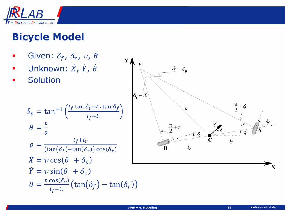