Embed Size (px)
Citation preview
arX
iv:1
710.
0730
6v2
[he
p-th
] 5
Mar
201
8
Towards formalization of the soliton counting technique for the
Khovanov–Rozansky invariants in the deformed R-matrix approach
A.Anokhina∗
ITEP/TH-29/17
Abstract
We consider recently developed Cohomological Field Theory (CohFT) soliton counting diagram tech-nique for Khovanov (Kh) and Khovanov–Rozansky (KhR) invariants [1, 2]. Although the expectationto obtain a new way for computing the invariants has not yet come true, we demonstrate that solitoncounting technique can be totally formalized at an intermediate stage, at least in particular cases. Wepresent the corresponding algorithm, based on the approach involving deformed R-matrix and minimalpositive division, developed previously in [3]. We start from a detailed review of the minimal positivedivision approach, comparing it with other methods, including the rigorous mathematical treatment [4].Pieces of data obtained within our approach are presented in the Appendices.
Contents
1 Introduction 21.1 Different appoaches to KhR invariants . . . . . . . . . . . . . . . . . . . . . . . . . . . . . . . 41.2 Conjectures and expectation s . . . . . . . . . . . . . . . . . . . . . . . . . . . . . . . . . . . . 4
2 A sketch of the general construction 42.1 The necessary notions of knot and representation theory . . . . . . . . . . . . . . . . . . . . . 42.2 Explicit expression for knot invariants . . . . . . . . . . . . . . . . . . . . . . . . . . . . . . . 82.3 Resolution hypercube . . . . . . . . . . . . . . . . . . . . . . . . . . . . . . . . . . . . . . . . 82.4 Vector spaces at the hypercube vertices . . . . . . . . . . . . . . . . . . . . . . . . . . . . . . 112.5 Spaces at the vertices as graded spaces . . . . . . . . . . . . . . . . . . . . . . . . . . . . . . . 122.6 From the resolution hypercube to the complex . . . . . . . . . . . . . . . . . . . . . . . . . . 132.7 Graded basis in the homologies . . . . . . . . . . . . . . . . . . . . . . . . . . . . . . . . . . . 142.8 The geometric meaning of the positive integer decomposition . . . . . . . . . . . . . . . . . . 14
3 Minimal positive division instead of computing the homology 153.1 General definitions . . . . . . . . . . . . . . . . . . . . . . . . . . . . . . . . . . . . . . . . . . 15
3.1.1 Complex, homologies and decomposition of the generating functions. . . . . . . . . . 153.1.2 Integer and polynomial division. . . . . . . . . . . . . . . . . . . . . . . . . . . . . . . 163.1.3 Division as homology computation . . . . . . . . . . . . . . . . . . . . . . . . . . . . . 17
3.2 “Ambigiuos” and “unambigiuos” minimal remainders . . . . . . . . . . . . . . . . . . . . . . . 173.3 Properties of maps as “selection rules” for the “minimal remainder” . . . . . . . . . . . . . . 18
3.3.1 Ranks of the differentials . . . . . . . . . . . . . . . . . . . . . . . . . . . . . . . . . . 183.3.2 Particular values of matrix elements . . . . . . . . . . . . . . . . . . . . . . . . . . . . 19
3.4 “Multilevel” division as a way to fix ambiguities . . . . . . . . . . . . . . . . . . . . . . . . . 20
4 Lie algebra structure in the complex and its breaking 204.1 The idea . . . . . . . . . . . . . . . . . . . . . . . . . . . . . . . . . . . . . . . . . . . . . . . . 214.2 Spaces in the resolution hypercube as representation spaces . . . . . . . . . . . . . . . . . . . 214.3 Are the homology spaces representation spaces? . . . . . . . . . . . . . . . . . . . . . . . . . . 22
4.3.1 A toy example . . . . . . . . . . . . . . . . . . . . . . . . . . . . . . . . . . . . . . . . 234.3.2 Relation to the real case . . . . . . . . . . . . . . . . . . . . . . . . . . . . . . . . . . . 23
∗ITEP, Moscow, Russia; [email protected]
1
5 Differential expansion and evolution method 245.0.1 The sketch of the methods . . . . . . . . . . . . . . . . . . . . . . . . . . . . . . . . . . 245.0.2 The interplay with the positive division method . . . . . . . . . . . . . . . . . . . . . . 245.0.3 The interplay with the group theory viewpoint . . . . . . . . . . . . . . . . . . . . . . 25
6 Minimal positive division approach and CohFT calculus 256.1 Preliminary comments . . . . . . . . . . . . . . . . . . . . . . . . . . . . . . . . . . . . . . . . 25
6.1.1 CohFT diagram technique . . . . . . . . . . . . . . . . . . . . . . . . . . . . . . . . . . 256.1.2 Selection rule for CohFT matrix elements . . . . . . . . . . . . . . . . . . . . . . . . . 256.1.3 Types of CohFT matrix elements and multilevel division . . . . . . . . . . . . . . . . . 266.1.4 Our program . . . . . . . . . . . . . . . . . . . . . . . . . . . . . . . . . . . . . . . . . 26
6.2 Division algorithm for a generic two strand knot . . . . . . . . . . . . . . . . . . . . . . . . . 266.2.1 The CohFT calculus in the two-strand case . . . . . . . . . . . . . . . . . . . . . . . . 266.2.2 Khovanov (N = 2) case . . . . . . . . . . . . . . . . . . . . . . . . . . . . . . . . . . . 276.2.3 KhR for generic N . . . . . . . . . . . . . . . . . . . . . . . . . . . . . . . . . . . . . 286.2.4 Primary polynomials as “deformed” HOMFLY polynomials . . . . . . . . . . . . . . . 286.2.5 Comparing the N = 2 and N > 2 cases . . . . . . . . . . . . . . . . . . . . . . . . . . 296.2.6 The primary polynomial as the generating function for the soliton diagrams . . . . . . 306.2.7 Example: torus knot T 2,5. . . . . . . . . . . . . . . . . . . . . . . . . . . . . . . . . . . 32
6.3 The first-level division for particular three-strand knots . . . . . . . . . . . . . . . . . . . . . 326.3.1 A draft of the three-strand reduction procedure . . . . . . . . . . . . . . . . . . . . . . 326.3.2 Explicit formulas for the three-strand (deformed) R-matrices . . . . . . . . . . . . . . 34
6.4 The generating function for the three-strand soliton diagrams . . . . . . . . . . . . . . . . . . 356.4.1 Guide to the experimental data . . . . . . . . . . . . . . . . . . . . . . . . . . . . . . . 35
7 Further directions 35
A Basic properties of the special point operators 38A.1 General constraints on the special point operators . . . . . . . . . . . . . . . . . . . . . . . . 38
A.1.1 Continuous space transformations and transformations of the knot diagram. . . . . . . 38A.1.2 Topological invariance constraints on the crossing and turning point operators. . . . . 39
A.2 Constraints on the R-matrices . . . . . . . . . . . . . . . . . . . . . . . . . . . . . . . . . . . 39A.3 Relations between the R and Q-matrices . . . . . . . . . . . . . . . . . . . . . . . . . . . . . . 39A.4 Properties of the particular solution . . . . . . . . . . . . . . . . . . . . . . . . . . . . . . . . 40A.5 Inverting of all crossings and mirror symmetry of the knot invariants . . . . . . . . . . . . . . 41
B The “graded” basis respected by the differentials 41
C Morphisms of the representation spaces. A more involved example 42
D List of braids providing the unique level I reminders 43
E Examples of the unique minimal remainders related to the CohFT diagrams in the caseof three strands 44E.1 The doubly twisted diagram of the unknot . . . . . . . . . . . . . . . . . . . . . . . . . . . . . 44E.2 The trefoil knot in different three strand presentations . . . . . . . . . . . . . . . . . . . . . . 45E.3 The “thick” knot 819 (torus T [3, 4]) . . . . . . . . . . . . . . . . . . . . . . . . . . . . . . . . . 50
1 Introduction
Cohomological knot invariants are rather young by knot theory standards. Khovanov invariants (denoted Khbelow) [5] were proposed less two decades ago and their Khovanov–Rozanski (KhR) version [4] was introducedless than a decade ago. Both approaches associate a function (precisely, a polynomial) to a knot (or a link),
2

Table 1: Constructively defined knot invariants
Knot diagram+representation of a Lie algebra
→Algebraic manip-ulations
→
Knot invariant: Alexander,Jones, HOMFLY, Kauffman,Vassiliev, coloured versions,. . .
Table 2: Homological knot invariants
The knotdiagram
Knot in-varinat
⇓ ⇑
Resolutionhypercube
⇒Sequence of linearspaces
⇒ Complex →Computingthe homology
& ?↑ &
Representationstructure onvertices
→Spaces asrepresentationspaces
?→
“Representation-friendly”nilpotentlinear maps
?→
Decomposingthe homology
↑ ?↓
Representation ofLie algebra
⇒ Standard construction→ Proposed conjecture?→ Particular cases analysed
“Differentialexpansion”for the knotinvariant
so that this function is invariant under arbitrary continuous space transformations. They belong to the wideand well-studied class of polynomial knot invariants [6, 7, 8], although drastically differing from the otherones in their properties. Differences between various knot invariants are illustrated in Tables 1 and 2.
The first and key special point of Khovanov, KhR and other invariants of the same kind [9] is a separatestructure associated with a knot, called knot homology. The knot polynomial is a generating function forthe basis vectors in homologies of a certain complex (and, even worse, in the KhR case the complex of othercomplexes). This sort of definition, which is multi-level and at many points implicit, causes severe obstaclesboth for general analysis and for explicit computations. Searches for an alternative approach are naturallyquite popular (see, e.g., the references in Table 3).
A closely related quantity is the superpolynomial of the knot [10], which remains among the most obscureissues of the knot theory. The superpolynomials are often studied together with the KhR invariants, theconnection being two-fold. On the one hand, the superpolynomial is by its only strict (yet not very practical)definition an analytic continuation of the KhR polynomial (similarly to the HOMFLY invariant, which is ananalytic continuation of the discrete set of polynomials generalising Jones polynomial1. On the other hand,alternative approaches developed for superpolynomials, although being neither general nor mathematicallystrict in the most cases, proved themselves highly useful both for computations and investigation of generalproperties of the theory. Hence, the interference of these two subjects may shed light on both super- andKhR polynomials.
A new inspiration in the subject comes from the recently proposed cohomological field theory [14],(“CohFT” henceforth) associated with Khovanonov and KhR invarinats in the same way as Chern-Simonstheory is associated with Jones and HOMFLY invarinats [15, 16, 17].
In the context of the recent progress of various approaches to the KhR invariants we wish to recall our
1However, the naively performed analytical continuation, working well in the HOMFLY case, runs into certain problems inthe KhR case [11, 12, 3, 13], see sec. 6.2.5, 7).
3
own research [3] and compare it with rigorous mathematical treatment, as well as with alternative methods,including the newly proposed CohFT approach.
Various issues concerned here, are summarized and supplied with bibliographic references in Table 3.The rightmost column of the table reflects the structure of the present text.
1.1 Different appoaches to KhR invariants
1.2 Conjectures and expectation s
All the viewpoints on the KhR invariants (or superpolynomials) differing from the original one generallyaim, speaking most strictly and naively, to obtain the desired invariants just by performing some algebraicmanipulations, i.e., to pass by the construction of the complex and the computation of the homologies. Inother words, one tries to invent a treatment more in the spirit of the standard knot invariant computations [6].
Because the KhR formalism applies to a complex of complexes, the expectation for its simplification lieson two levels,
1. The weak expectation : to find an explicit representation for the spaces and maps in the KhR complex.
In sec. 2 we suggest a way to do this relying on the R-matrix formalism (sec. 4 contains some furtherdetails). The same method was in fact implicitly used in [3].
2. The strong expectation : to skip computing the homologies.
This is the main idea of the minimal positive division technique, developed in [3] which we present insec. 3 in its abstract form. In 6 we attempt to combine it with the CohFT formalism from [2].
2 A sketch of the general construction
2.1 The necessary notions of knot and representation theory
Here we briefly review the necessary notions of the knot theory. Details can be found in any knot theorytextbook, e.g., in [6].
Oriented knot in R3. A knot K is by definition an embedding of the oriented circle (e.g., a counterclock-wise direction is selected) in the three-dimensional flat space
K : S1 → R3, (2.1)
considered up to continuous transformations of the space R3.
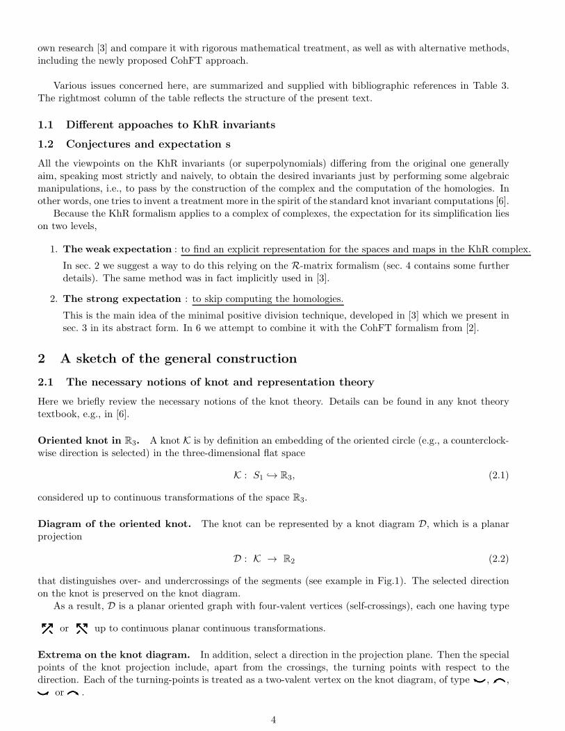
Diagram of the oriented knot. The knot can be represented by a knot diagram D, which is a planarprojection
D : K → R2 (2.2)
that distinguishes over- and undercrossings of the segments (see example in Fig.1). The selected directionon the knot is preserved on the knot diagram.
As a result, D is a planar oriented graph with four-valent vertices (self-crossings), each one having type
or up to continuous planar continuous transformations.
Extrema on the knot diagram. In addition, select a direction in the projection plane. Then the specialpoints of the knot projection include, apart from the crossings, the turning points with respect to thedirection. Each of the turning-points is treated as a two-valent vertex on the knot diagram, of type ■ , ✠ ,
✒or ❘ .
4

Table 3: Summary of the discussed approaches, with bibliographic and internal references
Khovanov polynomial N = 2
Introduced in [5]
Computational techniquedeveloped in
[18]
Table of results, together withcomputer code
[7] Presented for all prime knots(up to 11 crossings) and links(up to 11 crossings); in princi-ple, computed for any knots
Reviewed, e.g., in [19, 20], [21, 9]
Khovanov-Rozansky polynomial N ∈ Z+
The definition introduced in [4]
Applied to explicitcomputations in
[11] “Thin” knots up to 9 crossings
[22] Knots and links up to 6 cross-ings, mostly for particularvales of N
The appoach reviewed, e.g., in [21, 9]
Attemts of modification
Tensor-like formalism [23] Simplest examples, 2-strandtorus knots, twist knots
R-matrix bases formalism [3] 2 and 3-strand torus knots,3- and 4-strand knots andlinks up to 6 crossings, two-component links from two an-tiparallel strands
ssec. 2, 4
Positive division technique [3] ssec. 2.8, 3, 6
CoHFT approach [14, 1, 2] sec. 6
Superpolynomial 0 < N0 ≤ N ∈C
Introduced in [10]
Elvolution method [24], [25], [26] sec. 5
Differential expansion [12], [25], [27],[28], [29]
sec. 5
Finite N problem [11], [12], [3], [13] ssec. 6.2.5, 7
coloured generalizations [30], [24], [25],[27], [28], [31],[9],[32]
sec. 7
5
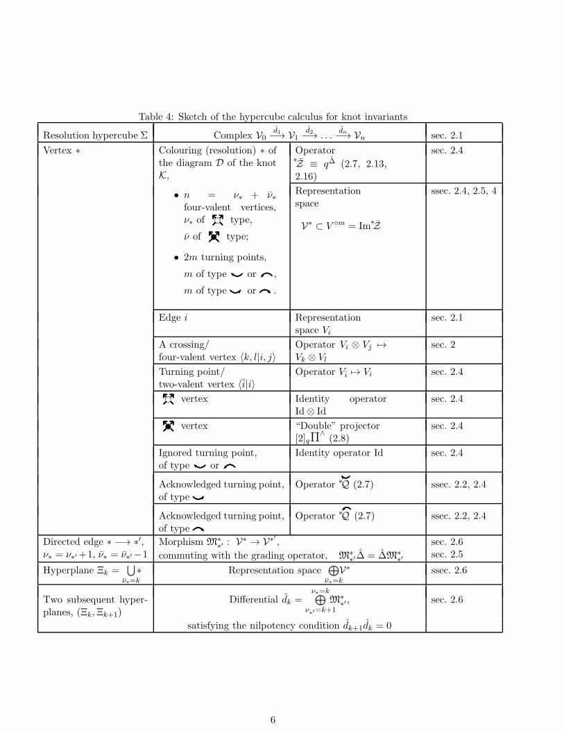
Table 4: Sketch of the hypercube calculus for knot invariants
Resolution hypercube Σ Complex V0d1−→ V1
d2−→ . . .dn−→ Vn sec. 2.1
Vertex ∗ Colouring (resolution) ∗ ofthe diagram D of the knotK,
Operator∗Z ≡ q∆ (2.7, 2.13,2.16)
sec. 2.4
• n = ν∗ + ν∗four-valent vertices,ν∗ of ❡ type,
ν of ✉ type;
• 2m turning points,
m of type ■ or ✠ ,
m of type✒
or ❘ .
Representationspace
V∗ ⊂ V ◦m = Im∗Z
ssec. 2.4, 2.5, 4
Edge i Representationspace Vi
sec. 2.1
A crossing/four-valent vertex 〈k, l|i, j〉
Operator Vi ⊗ Vj 7→Vk ⊗ Vl
sec. 2
Turning point/two-valent vertex 〈i|i〉
Operator Vi 7→ Vi sec. 2.4
❡ vertex Identity operatorId⊗ Id
sec. 2.4
✉ vertex “Double” projector[2]qΠ
∧(2.8)
sec. 2.4
Ignored turning point,of type ■ or ✠
Identity operator Id sec. 2.4
Acknowledged turning point,of type
✒
Operator ∗Q■ (2.7) ssec. 2.2, 2.4
Acknowledged turning point,of type ❘
Operator ∗Q✠
(2.7) ssec. 2.2, 2.4
Directed edge ∗ −→ ∗′,ν∗ = ν∗′ +1, ν∗ = ν∗′ −1
Morphism M∗∗′ : V∗ → V∗′ ,
commuting with the grading operator, M∗∗′∆ = ∆M∗
∗′
sec. 2.6sec. 2.5
Hyperplane Ξk =⋃
ν∗=k
∗ Representation space⊕
ν∗=k
V∗ ssec. 2.6
Two subsequent hyper-planes, (Ξk,Ξk+1)
Differential dk =ν∗=k⊕
ν∗′=k+1
M∗∗′ , sec. 2.6
satisfying the nilpotency condition dk+1dk = 0
6

r r
r
rr r
✠ ❘
❘
■✒ ✒Figure 1: Diagram of the figure-eight knot and the types of the crossings and turning points.
r
rr
r
r
r r ri i′ j′ j m m′
k′ p′l l′
i k′u u′
m′′ v′ v p
p′
m′′ m′
✠
✠❘
✒✠
✒ ■ ✒
++
— —
✠
❘ ✠
✒
✠
✒ ■ ✒Figure 2: Diagram that represents the same knot 41 as Fig.1 and contains only two kinds of crossings.
Representation space on the knot. The knot is associated with a representation space V of a Liealgebra g,
K → Y ∈ rep g (2.3)
i.e., one can imagine the linear space V suspended over each point of the knot. Then one can associate eachedge on the knot diagram with the space V .
Tensor representation for knot invariants. As a result, a two-valent vertex (a turning point) of theknot diagram can be related to a linear operator Q : V → V , and a four-valent vertex (a crossing) can berelated to a linear operator R : V ⊗ V → V ⊗ V .
The knot diagram as a diagram of the tensor contraction. The entire diagram D represents thenthe tensor contraction of these operators. To calculate this contraction explicitly, one should
1. Associate to each edge of D an integer valued label (the number of the basis vector in the space V ).
2. Multiply the components of R and Q corresponding to all the vertices.
3. Take the sum over all values of the labels (the summation sign is usually omitted in the formulas).
For some specially chosen operators R and Q, the tensor contraction related to the knot diagram turnsout to be a topological invariant. Discussing the corresponding constraints (briefly summarised in App. A)on the operators and their general solutions is beyond the scope of our survey. We just write down and usebelow all the needed explicit expressions.
7
2.2 Explicit expression for knot invariants
Here we present the key points of the R-matrix approach to knot invariants (proposed in [33, 34]; see, e.g.textbook [6], or either of the papers [35, 36, 37] for a detailed review).
Tensor contraction from knot diagram. The knot diagram must be drawn so that
• both arrows in each crossing have the projections on the preferred direction of the same sign.
In particular, the crossings never coincide with the turning points. One can bring any knot diagram tothe required form with the help of continuous planar transformations [6], e.g. the knot represented by thediagram in Fig. 1 is represented by the diagram in fig. 2 as well.
Then, the desired knot invariant is given by the expression2
H =∏
rj i
∗Q■ij
∏
rj i
∗Q✠ij
∏
ri j
∗Q■ij
∏
ri j
∗Q✠ij
∏
il
jk
+Rijkl
∏
jk
il
−Rijkl. (2.4)
E.g., knot diagram in Fig. 2 corresponds to the contraction
H(fig.2) =−Rj′i′
k′l
−Rl′p′
mj
+Rv′m′′
iu
+Ru′k′
pv∗Q■i
i′∗Q■j
j′∗Q■m
m′∗Q✠ll′
∗Q■u′
u∗Q✠v′
v∗Q✠pp′
∗Q✠m′
m′′ . (2.5)
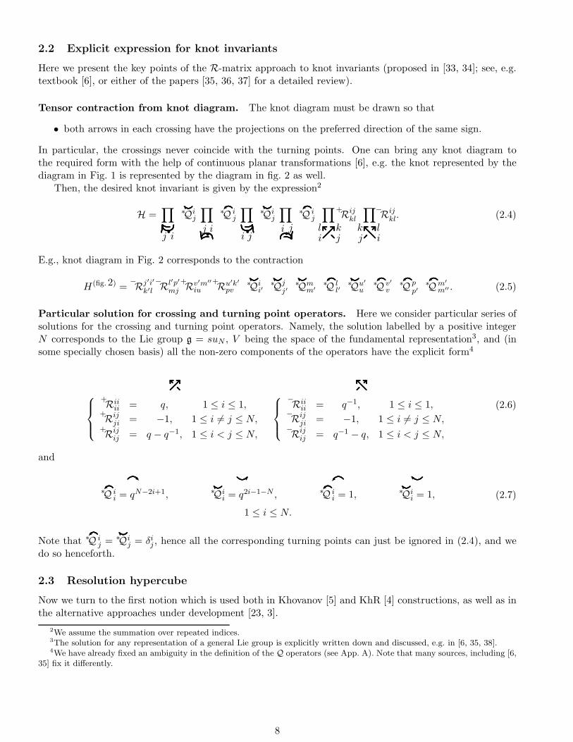
Particular solution for crossing and turning point operators. Here we consider particular series ofsolutions for the crossing and turning point operators. Namely, the solution labelled by a positive integerN corresponds to the Lie group g = suN , V being the space of the fundamental representation3, and (insome specially chosen basis) all the non-zero components of the operators have the explicit form4
+Riiii = q, 1 ≤ i ≤ 1,
+Rijji = −1, 1 ≤ i 6= j ≤ N,
+Rijij = q − q−1, 1 ≤ i < j ≤ N,
−Riiii = q−1, 1 ≤ i ≤ 1,
−Rijji = −1, 1 ≤ i 6= j ≤ N,
−Rijij = q−1 − q, 1 ≤ i < j ≤ N,
(2.6)
and
❘ ✒ ✠ ■∗Q✠ii = qN−2i+1, ∗Q■i
i = q2i−1−N , ∗Q✠ii = 1, ∗Q■i
i = 1,
1 ≤ i ≤ N.
(2.7)
Note that ∗Q✠ij =
∗Q■ij = δij , hence all the corresponding turning points can just be ignored in (2.4), and we
do so henceforth.
2.3 Resolution hypercube
Now we turn to the first notion which is used both in Khovanov [5] and KhR [4] constructions, as well as inthe alternative approaches under development [23, 3].
2We assume the summation over repeated indices.3The solution for any representation of a general Lie group is explicitly written down and discussed, e.g. in [6, 35, 38].4We have already fixed an ambiguity in the definition of the Q operators (see App. A). Note that many sources, including [6,
35] fix it differently.
8

V0 =
❝ ❝
❝ ❝1
V◦◦◦◦
1·1·1·1= 1
d0
❄
M◦◦◦◦◦◦◦•
✟✟✟✟✟✟✟✙
���✠
❅❅❅❘
❍❍❍❍❍❍❍❥
❝ ❝
❝ s
❝ ❝
s ❝
❝ s
❝ ❝
s ❝
❝ ❝
V1 =⊕
V◦◦◦•
1·1·1·q−1
= q−1
V◦◦•◦
1·1·q−1 ·1= q−1
V◦•◦◦
1·q ·1·1= q
V•◦◦◦
q ·1·1·1= q
T
d1
❄
✏✏✏✏✏✏✏✏✏✏✏✮
❍❍❍❍❍❍❥
PPPPPPPPPPPq
❝ ❝
s s
❝ s
❝ s
s ❝
❝ s
❝ s
s ❝
s ❝
s ❝
s s
❝ ❝
V2 =⊕
V◦◦••
1·1·q−1 ·q−1
= q−2
V◦•◦•
1·q ·1·q−1
= 1
V•◦◦•
q ·1·1·q−1
= 1
V◦••◦
1·q ·q−1 ·1= 1
V•◦•◦
q ·1·q−1 ·1= 1
V••◦◦
q ·q ·1·1= q2
T 2
d2
❄
PPPPPPPPPPPPq ❄
✏✏✏✏✏✏✏✏✏✏✏✏✮
❝ s
s s
s ❝
s s
s s
❝ s
s s
s ❝
V3 =⊕
V◦•••
1·q ·q−1 ·q−1
= q−1
V•◦••
q ·1·q−1 ·q−1
= q−1
V••◦•
q ·q ·1·q−1
= q
V•••◦
q ·q ·q−1 ·1= q
T 3
d3
❄
PPPPPPPPPq
❅❅❅❘
���✠
✟✟✟✟✟✟✟✟✙
s s
s s
V4 =V••••
q ·q ·q−1 ·q−1
= 1T 4
Figure 3: The resolution hypercube for the figure-eight knot (Fig. 2).
9

Decomposition for crossing operators. The operators (2.6) can be identically rewritten as linear
combinations of the identity operator and a projector (an operator Π∧such that Π∧Π∧
=Π∧), namely,
+R = q
◦R −
•R = qId⊗ Id − [2]qΠ
∧,
−R = q−1◦R −
•R = q−1Id⊗ Id − [2]qΠ
∧.
(2.8)
Formulas (2.8) do not follow from the general group theoretical and topological constraints. They are thespecial properties of the simplest solution to the constraints, which satisfies characteristic equations (A.9)(see App. A.4).
Hypercube representation for the knot invariant. If one substitutes the decomposition (2.8) of thecrossing operators in (2.4) and expands the product, the terms of the expansion are enumerated by variouscolourings ∗ ∈ {◦, •}n of the knot diagram, i.e., by the partitions of the ◦ and • signs (associated with twosummands in (2.8)) over the n crossings.
One can treat the types of crossings as the coordinates, ◦ = 0, • = 1. The expansion term associatedto the colouring ∗ thus corresponds to the point of n-dimensional space with coordinates ∗(◦ = 0, • = 1),so that all the 2n points form an n-dimensional hypercube. In turn, an edge (assumed to be directed) ofthe hypercube connects a pair of colourings related by a flip ◦ → •. A vertex ∗ ∈ perm{◦ . . . ◦
︸ ︷︷ ︸
ν∗
, • . . . •︸ ︷︷ ︸
ν∗
} is
then connected by ν∗ incoming and ν∗ = n − ν∗ outgoing arrows to the total of n vertices from the sets{∗′} = perm{◦ . . . ◦
︸ ︷︷ ︸
ν∗+1
, • . . . •︸ ︷︷ ︸
ν∗−1
} and {∗′′} = perm{◦ . . . ◦︸ ︷︷ ︸
ν∗−1
, • . . . •︸ ︷︷ ︸
ν∗+1
}, respectively.
As a result,
• Expression (2.4) for the knot invariant is expanded as a sum over the vertices of the directed graph,called a resolution hypercube5.
For example, Fig. 3 illustrates the hypercube for the diagram in Fig. 2.
The generating function for the colourings is defined as a formal series in the new variable T asfollows
Z(q, T ) ≡ Z(R(q) → R(q, T )
)=
∑
∗∈{◦,•}n
T ν∗∗Z, ν∗ = # {• ∈ ∗} , (2.9)
where∗Z stands for the expansion term related to the colouring ∗.
Expansion (2.9) is formally obtained from expression (2.4) for the knot invariant by substituting thecrossing operators with
+R(q, T ) ≡ q
◦R(q) + T
•R(q)
−R(q, T ) ≡ q−1◦R(q) + T
•R(q) ,
(2.10)
or, equivalently, their matrix elements with
Riiii 7→ q, 1 ≤ i ≤ 1,
Rijji 7→ T, 1 ≤ i 6= j ≤ N,
Rijij 7→ q + q−1T, 1 ≤ i < j ≤ N,
Rjiji 7→ q(1 + T ), 1 ≤ i < j ≤ N,
Riiii 7→ q−1, 1 ≤ i ≤ 1,
Rijji 7→ T, 1 ≤ i 6= j ≤ N,
Rijij 7→ q−1 + qT, 1 ≤ i < j ≤ N,
Rjiji 7→ q−1(1 + T ), 1 ≤ i < j ≤ N.
(2.11)
5In the graphical representation for the tensor contractions, the expansion terms are associated with the various resolutionsof the knot diagram.
10

2.4 Vector spaces at the hypercube vertices
The next step introduces representation theory data into the construction (see, e.g., [38] for the necessarybackground). The following presentation is equivalent to the standard presentation of the Khovanov con-struction [5] for the particular case of the su2 algebra (details can be found in [6]). It is very plausible thatthe KhR construction [4] in the more general case of suN is also reproduced, although in somewhat differentnotions6.
The operators related to a colouring. The∗Z contribution to (2.4), related to the colouring ∗ (with
ν∗ resolutions ◦, ν∗ resolutions •, n = ν∗ + ν− of them in total), identically equals to the contraction of two
operators (we omit the operators ∗Q✠ij =
∗Q■ij = δij). The first of these operators is given by
Q◦m∣∣I
J=∏
ri j
∗Q■ij
∏
ri j
∗Q✠ij (2.12)
where m is the number of the “left-to-right” turning points on the knot diagram7 (those are the only turningpoints one takes into account). The second operator is
∗ZIJ ≡ qν+−ν−
∏
❢il
kj
◦Rijkl
∏
✈il
kj
•Rijkl , ∗ ∈
{◦, •}n
, (2.13)
where we introduce the number ν+ (resp. ν−) of (resp. ) crossings resolved into◦R
ν+ = #
{
→ ❡ ∈D∗}
, ν− = #
{
→ ✉ ∈D∗}
. (2.14)
The power of q factor appears as a price for expressing both+R and
−R through the same pair
◦R and
•R.
The multi-indices I (resp. J) are defined as the sets of the labels attached to the edges coming in (resp.going out of) the turning points, i.e.,
I ={ ⋃
ri j
⋃
ri j
i}
, J ={ ⋃
ri j
⋃
ri j
j}
. (2.15)
Hence, both operators Q◦m and∗Z are defined on the tensor power V ◦m of the original space V , m being
the number of the “left-to-right” turning points in the knot diagram. In the following we also consider thecomposition of these two operators
∗Z ≡ QZ. (2.16)
Contraction (2.4) can then be equivalently presented as a trace
H = Tr V ◦mQZ = Tr V ◦mQ◦mZ = Tr V ◦mZ. (2.17)
6Two resolutions of a crossing in [4] are identified with two terms in the decomposition (2.8) for the suN R-matrix in thefundamental representation [38]. Then the spaces in the vertices of the resolution hypercube (and hence the spaces in theresulting complex), are described in [4] as the complexes of certain commutative polynomial rings. At the same time, thesecomplexes describe suN representation spaces in terms of the BGG resolvents [39]. The author is indebted to I. Danilenko forpointing out this observation and providing the reference.
7Then the knot diagram has 2m turning points in total. Indeed, the numbers of turning points of various kinds on a
closed curve satisfy
{
# {✠ }+# {❘ } = # {■
}+# {✒
}# {✠ }+# {
■} = # {❘ }+# {
✒}
, and the sum (resp. difference) of these equations yields
#✠ = #✒
(resp. #✠ = #✒
).
11

2.5 Spaces at the vertices as graded spaces
The Khovanov [5] and the KhR [4] constructions both essentially use one more notion related to represen-tation theory of quantum groups [38]. Namely, a special graded basis is considered in each vertex of thehypercube. Below we give the R-matrix description of these spaces implicitly used for explicit computationsin [3].
Spaces at the vertices as image spaces. One can show that8
∗Z(∗Z (V)
)=
∗Z (V) ⊂ V D, (2.18)
i.e., one can restrict the operator∗Z , originally defined on the space V ◦m, to its image where it acts as an
isomorphism:
∗Z : V∗ ≡ Im
∗Z∣∣V ◦m → V∗ (2.19)
Henceforth, we
• relate a colouring ∗ to the space V∗ defined by (2.19), with∗Z defined in (2.13, 2.16) and put this space
in the corresponding hypercube vertex.
Basis of eigenvectors as a graded basis. The operator∗Z has a basis of eigenvectors in the subspace
V∗, the eigenvalues being q powers,9
{X ∗α :
∗ZX ∗α = q∆αX ∗
α
}dimV∗
I=1. (2.20)
Hence, one can consider the linear space
v∗ ≡ span{q∆α
}. (2.21)
The contraction
P∗(q) ≡ Tr V∗∗Z (2.22)
is then the generating function for the basis of monomials in q. The two-variable generating function,
P(q, T ) ≡ H(R → R
)=∑
∗
T ν∗P∗(q). (2.23)
then coincides with the primary polynomial introduced in [3].
• Relations (2.22, 2.23) associate each term in the primary polynomial with a vector of the linear spaceplaced at one of the resolution hypercube vertices.
8 The operators∗R (∗ ∈
{
◦, •}
) defined in (2.8), satisfy∗R2 ∼
∗R, so that, if y ∈ Im
∗R, then y =
∗R2x =
∗Rx ∈
∗R(V ) and
hence the same is true for∗Z, which by definition (2.13) is a tensor product of the operators
∗R. The same is also true for the
operator∗Z = Q
∗Z, because Q
∗Z =
∗ZQ for any
∗Z (due to the “built in” representation theory properties of these operators [38])
so thatx = Q
∗Z(
Q∗Zy
)
= Q2∗Z2y ⇒ x = Q2∗Zz = Q
∗Z (Qy) ,
and∗Z (V) ≡ Q
∗Z (V) ⊂
∗Z−1V ⊂ V ⇒ V ⊂
∗ZV
The relations above imply that the operator∗Z is invertible. Hence,
∗Z (V) = V, as claimed.
9Similarly to the previous property, these facts follow from the definitions (2.13), (2.16) and the commutation relationQ∗Z =
∗ZQ.
12
2.6 From the resolution hypercube to the complex
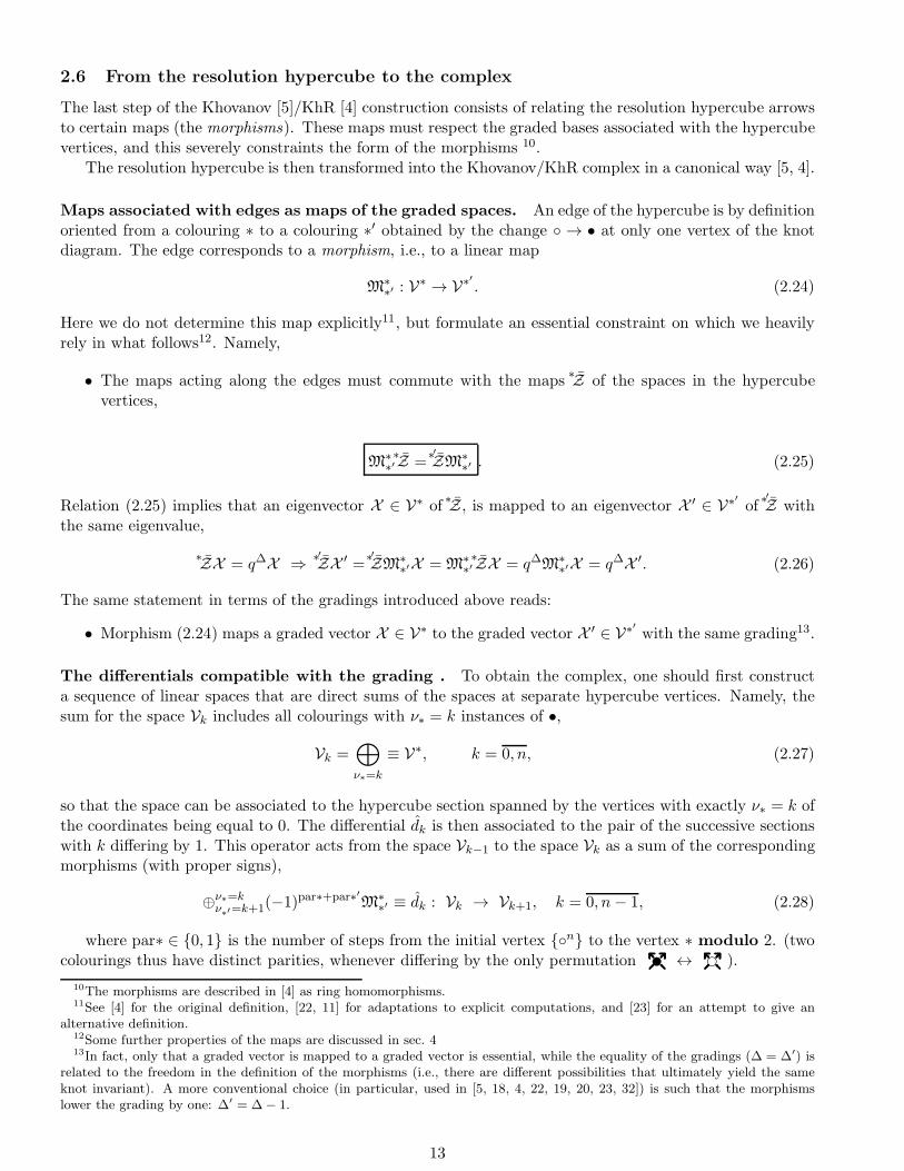
The last step of the Khovanov [5]/KhR [4] construction consists of relating the resolution hypercube arrowsto certain maps (the morphisms). These maps must respect the graded bases associated with the hypercubevertices, and this severely constraints the form of the morphisms 10.
The resolution hypercube is then transformed into the Khovanov/KhR complex in a canonical way [5, 4].
Maps associated with edges as maps of the graded spaces. An edge of the hypercube is by definitionoriented from a colouring ∗ to a colouring ∗′ obtained by the change ◦ → • at only one vertex of the knotdiagram. The edge corresponds to a morphism, i.e., to a linear map
M∗∗′ : V
∗ → V∗′ . (2.24)
Here we do not determine this map explicitly11, but formulate an essential constraint on which we heavilyrely in what follows12. Namely,
• The maps acting along the edges must commute with the maps∗Z of the spaces in the hypercube
vertices,
M∗∗′∗Z =
∗′ZM∗∗′ . (2.25)
Relation (2.25) implies that an eigenvector X ∈ V∗ of∗Z, is mapped to an eigenvector X ′ ∈ V∗′ of
∗′Z withthe same eigenvalue,
∗ZX = q∆X ⇒
∗′ZX ′ =
∗′ZM∗
∗′X = M∗∗′∗ZX = q∆M∗
∗′X = q∆X ′. (2.26)
The same statement in terms of the gradings introduced above reads:
• Morphism (2.24) maps a graded vector X ∈ V∗ to the graded vector X ′ ∈ V∗′ with the same grading13.
The differentials compatible with the grading . To obtain the complex, one should first constructa sequence of linear spaces that are direct sums of the spaces at separate hypercube vertices. Namely, thesum for the space Vk includes all colourings with ν∗ = k instances of •,
Vk =⊕
ν∗=k
≡ V∗, k = 0, n, (2.27)
so that the space can be associated to the hypercube section spanned by the vertices with exactly ν∗ = k ofthe coordinates being equal to 0. The differential dk is then associated to the pair of the successive sectionswith k differing by 1. This operator acts from the space Vk−1 to the space Vk as a sum of the correspondingmorphisms (with proper signs),
⊕ν∗=kν∗′=k+1(−1)par∗+par∗′M∗
∗′ ≡ dk : Vk → Vk+1, k = 0, n− 1, (2.28)
where par∗ ∈ {0, 1} is the number of steps from the initial vertex {◦n} to the vertex ∗ modulo 2. (twocolourings thus have distinct parities, whenever differing by the only permutation ✉ ↔ ❡ ).
10The morphisms are described in [4] as ring homomorphisms.11See [4] for the original definition, [22, 11] for adaptations to explicit computations, and [23] for an attempt to give an
alternative definition.12Some further properties of the maps are discussed in sec. 413In fact, only that a graded vector is mapped to a graded vector is essential, while the equality of the gradings (∆ = ∆′) is
related to the freedom in the definition of the morphisms (i.e., there are different possibilities that ultimately yield the sameknot invariant). A more conventional choice (in particular, used in [5, 18, 4, 22, 19, 20, 23, 32]) is such that the morphismslower the grading by one: ∆′ = ∆− 1.
13

The differentials defined by (2.28) are by construction nilpotent,
dkdk−1 = 0, k = 1, n, (2.29)
and commute with the colouring operators∗Z (because all the morphisms do),
Zk+1dk = dk+1Zk with Zk ≡⊕
ν∗=k
V∗. (2.30)
In other words,
• Starting from the resolution hypercube, the linear spaces at the vertices and the morphisms along thedirected edges, one constructs a sequence of spaces associated with entire hyperplanes and sequenceof nilpotent grading-preserving14 linear maps, the differentials. The resulting sequence provides thecomplex [40] associated with the knot diagram.
2.7 Graded basis in the homologies
In Eq. (2.20) we introduced graded bases in the hypercube vertices. There is, however, a freedom in thedefinition of such a basis: one can make a linear transformation mixing the vectors of the same grading.Below we describe a special basis, which is the union of the graded bases in the image, co-image and thehomology subspaces of the differentials in the complex. A more detailed derivation is given in B.
Nilpotency condition (3.2) implies that
x ∈ Im dk ⊂ Vkdef⇔ x = dky ⇒ x ∈ ker dk+1 ⊂ Vk+1
def⇔ dk+1x = 0 (2.31)
The converse is generally wrong. The homology space is by definition [40] the factor space
Hkdef== ker dk+1/dk ⊂ Vk+1, i.e., x ∈ Hk ⇔ dkx = 0 & dky 6= x, ∀y ∈ Vk, (2.32)
i.e., each vector x in the homology Hk is a kernel vector defined up to an arbitrary vector from the imagesubspace, x ∼ x + dky, ∀y ∈ Vk. Hence, one can identify the homology with any subspace Hk ∈ ker dk ofthe kernel such that dimHk = dimker dk − dim Im dk−1.
Just using the definitions we have the decomposition
Vk = Im dk ⊕ coIm dk+1 ⊕Hk, (2.33)
where x ∈ coIm ddef⇔ dx 6= 0.
A non-trivial consequence of the property (2.30) of the differentials is that
• Each of the three spaces in the decomposition (2.33) contains a graded basis.
Precisely, a basis in the space Vk can be composed of three groups of vectors (see App. B),
{
yk,i : dk+1yk,i 6= 0}dim Im dk+1
i=1∪
{
zk,i = dkyk−1,i
}dim Im dk
i=1∪{
hk,i
}dimVk−dim Im dk−dim Im dk+1
i=1,
∆yk,i = ∆k,iyk,i ∆zk,i = ∆k−1,izk,i ∆hi,k = ∆′i,khi,k.
(2.34)
2.8 The geometric meaning of the positive integer decomposition
Here we address the final issue of this section, namely the derivation of the positive integer decompositionfor the primary polynomial from [3].
14See the above footnote in the definition of the morphisms.
14

Calculating the trace (2.17) in the basis (2.34) yields the following decomposition of the generatingfunction
P(q, T ) =
n∑
k=0
T kTr Vkq∆ ≡
n∑
k=0
T kdim qV =
n∑
k=0
T k(
Tr coIm dk+1q∆ +Tr Im dk
q∆ +TrHkq∆)
(2.34)==
=
n∑
k=0
T k
dim Im dk+1∑
i=1
q∆k,i +
dim Im dk∑
i=1
q∆k−1,i +
dimHk∑
i=1
q∆′k,i
=
=
n−1∑
k=0
(
T k + T k+1) dim Im dk+1∑
i=1
q∆k,i +
n∑
k=0
T kdimHk∑
i=1
q∆′k,i = (1 + T )J (q, T ) + P(q, T ). (2.35)
Note that the coefficient of each power q∆, both in J (q, T ) and P(q, T ), as well as in P(q, T ), is nothingbut the multiplicity of the basis vector from the corresponding subspace (⊕n
k=1Im dk, ⊕nk=0Hk or ⊕n
k=0Vk,respectively) with the grading ∆. This leads to the essential property of the obtained decomposition,
• All three quantities in decomposition (2.35), the dividend P(q, T ), the quotient J (q, T ) and theremainder P(q, T ) are sums of the q and T powers with positive integer coefficients.
3 Minimal positive division instead of computing the homology
In this section, we wish to discuss the positive integer division approach as a shortcut in general homologycomputations, without reference to the knot theory applications.
Through the section, the spaces V , the maps d and all the related quantities are not associated anyhowwith the particular complexes arising from the knot theory. Here we do not consider graded linear spaces,since a graded complex (see sec. 2.5) is always a direct sum of ordinary complexes. Also we do not considerany additional structures on the linear spaces, such as the structure of Lie algebra representation (this isthe case of the next section, sec. 4).
3.1 General definitions
3.1.1 Complex, homologies and decomposition of the generating functions.
Despite the fact that the most relevant definitions and theorems have already been given above, in sec. 2,we present them below in a compressed form for convenience.
Generally, a complex [40] is defined as a sequence of linear spaces and linear maps,
0d0−→ V0
d1−→ V1d2−→ V2
d3−→ . . .dn−→ Vn
dn+1−→ 0, (3.1)
such that any pair of the subsequent maps satisfies the nilpotency condition:
d2d1 = d3d2 = . . . = dndn−1 = 0. (3.2)
Condition (3.2) in particular implies that Im dk ⊂ ker dk+1 (k = 0, n).The homology in term k is the factor space
Hk ≡ ker dk+1/Im dk, (3.3)
which can be understood as a subspace of kernel vectors, in which any two vectors differing by an imagevector are treated as the same homology element,
x ∈ Hk ⇒ dk+1x = 0, (3.4)
x ∼ y ∈ Hk ⇐ x− y = dkz
((3.2)⇒ dk+1x = dk+1y = 0
)
.
15

The generating functions
F ≡n∑
k=0
T kdimVk, J (T ) ≡n∑
k=0
T kdim Im dk, P ≡n∑
k=0
T kdimHk (3.5)
in formal variable T for the dimensions of the linear spaces, the image subspaces and the homologies satisfythe relation (a particular case of (2.35), when q = 1 so that dim q → dim )
F(T ) = P(T ) + J (T )(1 + T ). (3.6)
The function P(T ) is referred to as the Poincare polynomial of the complex; in particular, χ ≡ P(T = −1)is the Euler character of the complex. In the following, we call (3.6) a positive integer decomposition for thegenerating function, because
• All the coefficients of the T powers in F(T ), P(T ) and J (T ) are by definition positive integer numbers(the dimensions of the corresponding subspaces).
We study the following question:
• To what extent can one recover the remainder P(T ) from the dividend F(T ) avoiding the straight-forward computing the homology?
The realization of the Strong expectation formulated in sec. 1.2 is associated with the progress along thisway.
Treated as an isolated algebraic problem, the above question can possess no satisfactory answer, notbeing even formulated rigorously. Below we attempt to formulate the problem more precisely, employingvarious additional considerations.
3.1.2 Integer and polynomial division.
The polynomial division is a straightforward extension of the integer division15. Both problems are formu-lated in the table below (the given quantities are underlined, the quantities to be determined are markedby the question sign).
Integer division Polynomial division (variable T )
m,k, q, p ∈ Z F(T ), G(T ), J (T ), P(T ) ∈ Pol(T )
m = k · q + p F(T ) = G(T ) · J (T ) + P(T )dividend divisor quotient remainder dividend divisor quotient remainder
? ? ? ?
ambiguity constraint ambiguity
k → q + u, p → p− ku, u ∈ Z 0 ≤ p < q J → J + f(T ), P → P − f(T )Q, f(T ) ∈ Pol(Z|T )
(3.7)
In both cases the equality in the third row does not define the unknown quantity uniquely. Namely, theequality still holds if both the quotient and the remainder are subjected to the transformation in the lastrow. In the integer case, the ambiguity is conventionally fixed by the constraint given in the same line. Thepolynomial case is essentially distinct at this point. Namely, none of the formal ways to select the uniqueremainder (now defined up to a polynomial instead of just an integer) a priory produces a quantity adequatefor our purposes.
15It is in fact the multivariable division, which is applied to the KhR calculus, but we do not discuss this generalization here.
16

3.1.3 Division as homology computation
Now we give an elementary illustration of the main idea we use, namely of the correspondence between thehomology calculus and the polynomial division, with a freedom in definition of the remainder (see the lastline in Tab. 3.7 and the comment in the end of sec. 3.1.2). Below we take a simple particular case of divisionproblem, and construct two different complexes with the homologies producing two different remainders.
In the context of knot polynomials (see sec. 6), we in fact deal with the very special case of the rightcolumn of Tab. 3.7, when all the polynomials have only positive integer coefficients, and the divisor is thebinomial (1 + T ). The general problem we consider is to present a given polynomial F(T ) in the form
F(T ) = (1 + T )J (T ) + P(T ) (3.8)
F(T ) =n∑
k=0
akTk, J (T ) =
m∑
k=0
bkTk, P(T ) =
l∑
k=0
ckTk, {ak, bk, ck} ⊂ Z+.
Large freedom in the definition of the remainder yet remains even in this particular case, as we will see inthe examples below.
In the particular case described below the division problem is straightforwardly related to the problemof computing the homologies. Namely, extracting the ∼ (1+T ) part is equivalent to matching the monomialterms in the pairs (x, Tx), each monomial entering only one pair. Some monomials remain unpaired andrepresent the homologies. E.g., F(T ) = 3+4T+T 2 admits two matchings, each with one unpaired monomial,
3 + 4T + 2T 2 =
3 + 3T+ T + T 2
• ✲ • + T 2
• ✲ •
• ✲ • d1d0 • ✲ •
•
(1 + T ) · (3 + T ) + T 2
1 +2 + 2T• + 2T + 2T 2
• ✲ •
• ✲ • d1d0 • ✲ •
• ✲ •
1 + (2 + 2T ) · (1 + T )
(3.9)
In either diagram in (3.9), a bullet is placed in the column (k + 1) for each T k term in F ; the arrowslabel the matching pairs. The positions of the arrows matching column k with column (k + 1) can thenbe represented by the matrix dk−1 such that dijk−1 = 1 if bullet i in column k matches bullet j in column
(k + 1), and dijk−1 = 0 otherwise. Then, the two particular diagrams in (3.9) give rise to the matrices
d1 =
(0 0 0 10 0 0 0
)
, d0 =
1 0 00 1 00 0 10 0 0
, and d1 =
(0 0 1 00 0 0 1
)
, d0 =
0 1 00 0 10 0 00 0 0
. (3.10)
In both cases d1d0 = 0, since each bullet enters no more than one pair. Hence, if a column is associated with alinear space (and bullet with a basis vector), the arrows define the differentials with the matrices (3.10). Onethus obtains the complex, with the homology spanned by the basis vectors corresponding to the unpairedbullet (related to the remainder in the division problem).
3.2 “Ambigiuos” and “unambigiuos” minimal remainders
As already discussed in sec. 3.1.2, decomposition (3.8) is not unique. The first and the most naive constraintwe impose on the remainder is
• The remainder P(T ) contains the minimal possible number of different T powers.
17

Although this requirement defines the unique remainder only in particular cases, it turns out to be veryuseful in application to knot polynomials (see [3] and sec. 6). Moreover, all further more involved constraintswill be developments of this elementary one.
Below we consider in details the simplest examples, when F(T ) contains up to three subsequent Tpowers16. The ambiguity in the remainder depends on the coefficients in the dividend. Explicit relationsare provided in Tabs.17 (3.11–3.12) (3.11), (3.12). As one can see from Tab. (3.12), already the case of thethree-term dividend appears to be rather non-trivial.
F(T ) = aT k
Type Unambigious
J (T ) 0
P(T ) a0Tk
F(T ) = a0 + a1T, χ ≡ a0 − a1
Type Unambigious
Case χ > 0 χ = 0 χ < 0
χ+ a1(1 + T ) a0(1 + T ) (−χ)T + a0(1 + T )
J (T ) a1 a0 = a1 a0
P(T ) χ 0 (−χ)T
(3.11)
F(T ) = a0 + a1T + a2T2, χ ≡ a0 − a1 + a2
Type Unambigious Ambigious
Case χ ≤ 0 χ > 0
a0 ≤ a1 < a2 a2 ≤ a1 < a0 a1 < a0, a1 < a2 a0 ≤ a1, a2 ≤ a1
J (T ) a0 + a2T a0 + (a1 − a0)T (a1 − a2) + a2T (a0 − p) + (p − a0 + a1)T(a1 − a2) + a2T ;a0 + (a1 − a0)T
P(T ) (−χ)T χT 2 χ p+ (χ− p)T 2 χ;
0 < a0 − a1 ≤ p ≤ a0 < χ χT 2
E.g. 1 + 3T + T 2 1 + T + 2T 2 2 + T + T 2 3 + 2T + 4T 2 = 3 + 4T + 2T 2 =
= T+ = T 2+ = 1+(1 + 4T 2
)+ 2(1 + T ) T 2 + (1 + T )(1 + 2T )
(1 + T )2 (1 + T )2 (1 + T )2 =(2 + 3T 2
)+ (1 + T )2 = 1 + 2(1 + T )2
(3.12)
3.3 Properties of maps as “selection rules” for the “minimal remainder”
In this section we recall the homology computation problem (formulated in Sec. 3.1.1) underlying the minimalpositive division problem we consider (formulated in Sec. 3.1.2). Below we explore, in the simplest cases,how the particular known properties of the differentials may help to determine the “minimal remainder”,when it is ambiguous.
3.3.1 Ranks of the differentials
The maps d in complex (3.1) can not be isomorphisms for generic dimensions of the spaces V . E.g., in thecase of a two-term complex,
0d0−→ V0
d1−→ V1d2−→ 0, (3.13)
the rank of the only non-zero map d1 must satisfy
rank d1 ≡ dim Im d1 ⊆ V1 ≤ min(dimV0,dimV1). (3.14)
16If the T powers are not subsequent, i.e., ak = 0 for some k, then problem (3.8) should be solved separately for the polynomials
F ′(T ) =k−1∑
k′=0
ak′ and F ′′(T ) =n∑
k+1
ak′ (such that F(T ) = F ′(T ) + F ′′(T )); this is a consequence of the positive coefficients
requirement.17In the latter two cases we omit the inessential T power factor in F by setting the smallest T power to zero.
18

Starting from the next case of a three-term complex,
0d0−→ V0
d1−→ V1d2−→ V2
d3−→ 0, (3.15)
the nilpotency condition also becomes non-trivial, producing additional constraints. In particular, d2d1 = 0implies that
Im d1 ⊂ ker d2 ⇒ rank d1 ≡ dim Im d1 ≤ dimker d2 = dimV1 − dim Im d2 ≡ dimV1 − rank d2, (3.16)
i.e.,
rank d1 + rank d2 ≤ dimV1, (3.17)
and also
rank d1 ≤ min (dimV0,dim V1) , rank d2 ≤ min (dimV1,dimV2) , (3.18)
similarly to the previous case.The ranks of the differentials for various choices of minimal remainders in the division problem (3.11–
3.12) are given in Tables (3.19), (3.20) (we omit the trivial one-term case).
dimV0 = v0, dimV1 = v1, χ = v0 − v1Case χ > 0 χ = 0 χ < 0
max rank d1 v0 v0 = v1 v1
mindimH0 ⊂ V0 0 0 −χ
mindimH1 ⊂ V1 χ 0 0
(3.19)
dimV0 = v0, dimV1 = v1, dimV2 = v2, χ = v0 − v1 + v2
Case χ ≤ 0 χ > 0
v0≤v1<v2 v2≤v1<v0 v1<v0, v1<v2 v0≤v1, v2≤v1
rank d1 v0 v0 v1 − v2 v0 − p v1 − v2 v0
rank d2 v2 v1 − v0 v2 p− v0 + v1 v2 v1 − v0
dimH0 0 0 χ 0<v0 − v1≤p ≤ v0 χ 0
dimH1 −χ 0 0 0 0 0
dimH2 0 χ 0 0<v2 − v1≤χ− p 0 χ
(3.20)
3.3.2 Particular values of matrix elements
More detailed data include the values of the particular matrix elements. To determine explicitly just severalof them it is sufficient to determine the ranks of the differentials, and hence the “minimal remainder”. Forexample,
rank(k k
)=
{0, k = 01, k 6= 0
; rank
(1 −1 k−1 1 p
)
=
{0, k + p = 01, k + p 6= 0
(3.21)
However, the general case is different, e.g.,
∀k rank(1 k
)= 1; ∀k rank
(1 −1 k−1 1 1− k
)
= 2; ∀k rank
(1 −1 k−1 1 −k
)
= 1;
∀k, p rank
(1 0 k0 1 p
)
= 2.
(3.22)
19

3.4 “Multilevel” division as a way to fix ambiguities
A further “improvement” consists in artificially splitting the initial division problem into two (or more)levels. Namely, suppose the original polynomial is given in the form of the decomposition (the summationindex Y running over a given set of values)
F(T ) =∑
Y
FY (T )CY (T ). (3.23)
Then, the division can be first performed for each FY (T ) separately, and then for the linear combinationsof the resulting remainders, namely
I. FY (T ) = PY (T ) + (1 + T )JY (T ). (3.24)
II. PI(T ) ≡
∑
CY (T )PY (T ) = PII(T ) + (1 + T )J
II(T ). (3.25)
The simplest example below illustrates how such “multilevel” division may fix an ambiguous remainder.Let G(T ) = 1 + T and
Y 1 2
CY 1 T 2
FY 1 + T 1
, (3.26)
so that F(T ) admits two positive integer decompositions, both with the monomial remainder,
F(T ) = F1C1 + F2C2 = 1 + T + T 2 = 1 + (1 + T ) · T = T 2 + 1 · (1 + T ). (3.27)
From the viewpoint of the multilevel division, one decomposition is preferred, namely,
I. F1 = 0 + 1 · (1 + T ) ⇒ P1 = 0,
F2 = 1 + 0 · (1 + T ) ⇒ P2 = 1.
II. P = P1C1 + P2C2 = 0 · 1 + 1 · T 2 = T 2 + 0 · (1 + T ) ⇒ PII= T 2 . (3.28)
The suggested algorithm is motivated by the known properties of the knot polynomials, see [3] and sec. 5.
4 Lie algebra structure in the complex and its breaking
In this section, we return to the particular complex that arises in the context of knot invariants, associatedwith the resolution hypercube (see sec. 2.3), and discuss in some further details the spaces at the verticesand the morphsims along the edges.
Namely, we slightly touch the topic of representation theory structures associated with the resolutionhypercube, with the constructed complex, and with the obtained knot invariants. Although at the momentwe are able neither to present a closed construction, nor to extract any practical output, we see at least tworeasons for addressing this subject.
First, the description of the spaces and differentials in the original KhR formalism [4, 22] refers to the
representation theory (see ssec. 2.4–2.6, especially footnote6.). In particular, it looks highly plausible thatthe representation theory properties of the morphisms determine their particular form to much extend.
Second, the known properties of the resulting knot invariants, which are the KhR invariants, as well asthat of the closely related superpolynomials [10, 12], might have a natural representation theory interpreta-tion. Moreover, it seem that this structure becomes more transparent, from the viewpoint of the differentialexpansion technique [28], and the evolution method [25] (see sec. 5).
In this section, we use a number of representation theory notions and statements without any comments,referring the reader to [38], whenever necessary. The most necessary notions are contained in the following
20

Quick reference. Standard basis in the Lie algebra and in the representation space. Bydefinition, the Lie algebra g is a linear space (usually over complex numbers) with the additional operation(the commutator). I.e., any pair of elements A1 and A2 of the algebra correspond an element [A1, A2] of thealgebra. Here we consider only simple finite dimensional Lie algebras.
In this case all elements of an algebra g can be obtained from the 2r generators, by taking successivelythe commutators and linear combinations of the elements. The generators include lowering operators Eαand the raising operators Fα, with α = 1, r.
A representation of the algebra is a linear map of the algebra to the space of linear operators consistentwith the definition of the commutator. These linear operators act in the representation space V of thealgebra. Throughout the text we consider the algebra together with its representation and do not make adifference between the algebra elements and the corresponding linear operators.
We consider only the finite-dimensional representations of simple Lie algebras. All these representationsare highest weight representations. This means that the representation space contains the special basiscomposed of the highest vector X∅ ≡ X, which is annihilated by all the raising operators (FαX = 0, α = 1, r)and the maximum linearly independent subset of descendant vectors X{α} = Eα1
. . . Eαkx, obtained from
the successive action of the lowering operators on x. The vectors X{α} are the common eigenvectors of theCartan operators Hα = [Eα, Fα], i.e., HαX{β} = Λα{β}X{β} for all possible α and {β}.
For further details see, e.g., [38].
4.1 The idea
As we discussed in sec. 2, both the HOMFLY and the KhR invariants can be considered as the generatingfunctions for the graded bases in the spaces in the Khovanov complex and in its homologies, respectively.The HOMFLY invariant is explicitly expressed through the R-matrices, associated with certain Lie algebrarepresentations, and can be expanded over the characters of these representations. This is not true forthe KhR invariant. Yet, in particular cases these invariants can be expressed via some remnants of therepresentation theory structure that governs the HOMFLY polynomial [12], [25], [27], [28], [29], [23], [3], [?].This phenomenon finds a natural explanation, if the spaces Vk in the KhR complex are representation spacesof the Lie algebra, while the homologies are not. At the same time the latter ones can be invariant spacesof some subalgebra. In turn, this happens if the morphisms in the complex commute with this subalgebra,but not with the entire algebra.
4.2 Spaces in the resolution hypercube as representation spaces
In sec. 2 we describe the space V∗ ⊂ V ◦m at the hypercube vertex ∗ as a subspace of the tensor power ofthe representation space V initially associated with the knot (the power m is half the number of the turning
points on the knot diagram, see ssec. 2.4–2.5 including the footnote7). Precisely, these spaces are defined asinvariant spaces of the grading operator
∗Z, which allows one to introduce the graded basis∗Z of eigenvectors
in each of these spaces (see tab. 4 for the basic formulas and for the general plan of the construction). Eachspace Vk in the complex is in turn defined as a direct sum of several V∗; hence, the Vk is an invariant spaceof
∗Z and has a graded basis as well. In this section, we consider an even stronger claim that
• The spaces in the complex constructed for a given knot are representation spaces of the Lie algebra g
associated with the knot.
Note that V∗ is generally a reducible representation.The above claim follows from the definition (2.12–2.16) of the operator
∗Z, which is a contraction of theoperators Q and R, and from the representation theory properties of these operators [38] (see also App. A).
The derivation is similar to the reasoning in footnote8.Since Q and R, and hence
∗Z commute with all the elements of the algebra, i.e.,
A∗Z =
∗ZA, ∀A ∈ g, ∗ ∈
{◦, •}n
, (4.1)
21
then
∀x ∈ V∗(
⇔ x =∗Zy)
⇒ Ax =∗Z(Ay) ∈ V∗. (4.2)
Hence, by definition, V∗ is the representation space of g, and the same is true for the sums of V∗ that yieldVk.
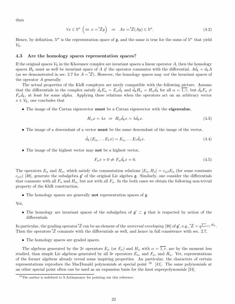
4.3 Are the homology spaces representation spaces?
If the original spaces Vk in the Khovanov complex are invariant spaces a linear operator A, then the homologyspaces Hk must as well be invariant space of A if the operator commutes with the differential, Adk = dkA(as we demonstrated in sec. 2.7 for A =
∗Z). However, the homology spaces may not the invariant spaces of
the operator A generally.The actual properties of the KhR complexes are nicely compatible with the following picture. Assume
that the differentials in the complex satisfy dkEα = Eαdk and dkHα = Hαdk for all α = 1, r, but dkFα 6=Fαdk, at least for some alpha. Applying these relations when the operators act on an arbitrary vectorx ∈ Vk, one concludes that
• The image of the Cartan eigenvector must be a Catran eigenvector with the eigenvalue,
Hαx = λx ⇒ Hαdkx = λdkx. (4.3)
• The image of a descendant of a vector must be the same descendant of the image of the vector,
dk (Eαi. . . E1x) = Eαi
. . . E1dkx. (4.4)
• The image of the highest vector may not be a highest vector,
Fαx = 0 6⇒ Fαdkx = 0. (4.5)
The operators Eα and Hα, which satisfy the commutation relations [Eα,Hβ] = cαβEα (for some constantscαβ) [38], generate the subalgebra g′ of the original Lie algebra g. Similarly, one consider the differentialsthat commute with all Fα and Hα, but not with all Fα. In the both cases we obtain the following non-trivialproperty of the KhR construction,
• The homology spaces are generally not representation spaces of g.
Yet,
• The homology are invariant spaces of the subalgebra of g′ ⊂ g that is respected by action of thedifferentials.
In particular, the grading operator∗Z can be an element of the universal enveloping [38] of g′, e.g.,
∗Z = q
∑rα=1Hα .
Then the operators∗Z commute with the differentials as well, and hence in full consistence with sec. 2.7,
• The homology spaces are graded spaces.
The algebras generated by the 2r operators Eα (or Fα) and Hα with α = 1, r, are by the moment lessstudied, than simple Lie algebras generated by all 3r operators Eα, and Fα, and Hα. Yet, representationsof the former algebras already reveal some inspiring properties. An particular, the characters of certainrepresentations reproduce the MacDonald polynomials at special point 18 [41]. The same polynomials atan other special point often can be used as an expansion basis for the knot superpolynomials [24].
18The author is indebted to S.Arthamonov for pointing out this reference.
22
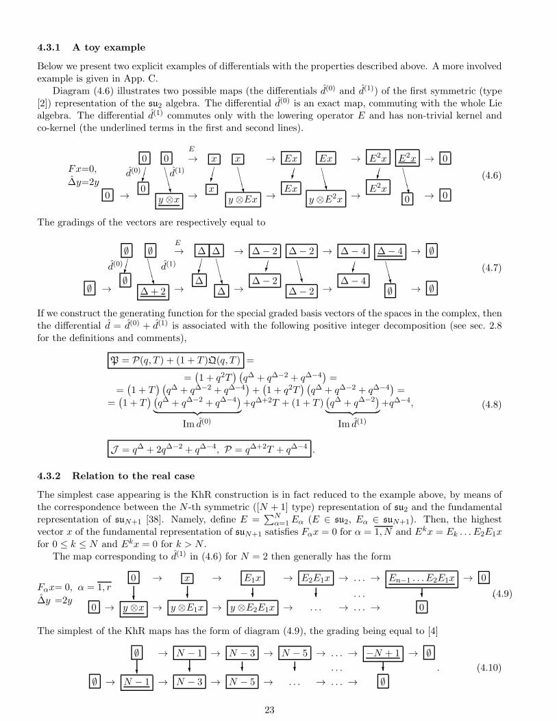
4.3.1 A toy example
Below we present two explicit examples of differentials with the properties described above. A more involvedexample is given in App. C.
Diagram (4.6) illustrates two possible maps (the differentials d(0) and d(1)) of the first symmetric (type[2]) representation of the su2 algebra. The differential d(0) is an exact map, commuting with the whole Liealgebra. The differential d(1) commutes only with the lowering operator E and has non-trivial kernel andco-kernel (the underlined terms in the first and second lines).
Fx=0,
∆y=2y
E
0 0 → x x → Ex Ex → E2x E2x → 0
d(0) ✄✄✎
❈❈❈❲
d(1) ✄✄✎
❈❈❈❲
✄✄✎ ❈❈❈❲
✄✄✎ ❈❈❈❲0 x Ex E2x
0 → → → → → 0y ⊗x y ⊗Ex y ⊗E2x 0
(4.6)
The gradings of the vectors are respectively equal to
E
∅ ∅ → ∆ ∆ → ∆− 2 ∆− 2 → ∆− 4 ∆− 4 → ∅
d(0) ✄✄✎❈❈❈❲
d(1) ✄✄✎
❈❈❈❲
✄✄✎ ❈❈❈❲
✄✄✎ ❈❈❈❲∅ ∆ ∆− 2 ∆− 4
∅ → → → → → ∅∆+ 2 ∆ ∆− 2 ∅
(4.7)
If we construct the generating function for the special graded basis vectors of the spaces in the complex, thenthe differential d = d(0) + d(1) is associated with the following positive integer decomposition (see sec. 2.8for the definitions and comments),
P = P(q, T ) + (1 + T )Q(q, T ) =
=(1 + q2T
) (q∆ + q∆−2 + q∆−4
)=
=(1 + T
) (q∆ + q∆−2 + q∆−4
)+(1 + q2T
) (q∆ + q∆−2 + q∆−4
)=
=(1 + T
) (q∆ + q∆−2 + q∆−4
)
︸ ︷︷ ︸
Im d(0)
+q∆+2T + (1 + T )(q∆ + q∆−2
)
︸ ︷︷ ︸
Im d(1)
+q∆−4,
J = q∆ + 2q∆−2 + q∆−4, P = q∆+2T + q∆−4 .
(4.8)
4.3.2 Relation to the real case
The simplest case appearing is the KhR construction is in fact reduced to the example above, by means ofthe correspondence between the N -th symmetric ([N + 1] type) representation of su2 and the fundamentalrepresentation of suN+1 [38]. Namely, define E =
∑Nα=1 Eα (E ∈ su2, Eα ∈ suN+1). Then, the highest
vector x of the fundamental representation of suN+1 satisfies Fαx = 0 for α = 1, N and Ekx = Ek . . . E2E1xfor 0 ≤ k ≤ N and Ekx = 0 for k > N .
The map corresponding to d(1) in (4.6) for N = 2 then generally has the form
Fαx= 0, α = 1, r
∆y =2y
0 → x → E1x → E2E1x → . . . → En−1 . . . E2E1x → 0
❄ ❄ ❄ ❄ . . . ❄
0 → y ⊗x → y ⊗E1x → y ⊗E2E1x → . . . → . . . → 0
.(4.9)
The simplest of the KhR maps has the form of diagram (4.9), the grading being equal to [4]
∅ → N − 1 → N − 3 → N − 5 → . . . → −N + 1 → ∅
❄ ❄ ❄ ❄ . . . ❄
∅ → N − 1 → N − 3 → N − 5 → . . . → . . . → ∅
. (4.10)
23

5 Differential expansion and evolution method
5.0.1 The sketch of the methods
Now we briefly outline two more (highly interrelated) approaches to the KhR (and super-) polynomials.These two approaches are the evolution method [24, 25, 26] and the differential expansion19 [12, 25, 27,28, 29]. Some grounds for these approaches are given by recently obtained recurrent relations for the KRpolynomials. In some cases these relations are derived from the Khovanov/KhR construction (essentially,from the exact skein triangle) [42, 43], while in other cases they remain an empiric observation. Hence,at the moment neither the differential expansion, nor the evolution method are based on any rigorouslyformulated construction. Yet both methods are highly effective as computational tools.
All three approaches—positive division, differential expansion and evolution method—share more incommon with each other than with the original KhR construction. We include this issue in this sectionto emphasize the possible (as yet mostly empiric) relation of these approaches to Lie group representationtheory. We complete the discussion by comparing the two approaches with the positive division approach(an interplay was already observed in [3]).
In both the evolution and the differential expansion methods one studies an entire family of knots insteadof its single representative. The family can be either relatively general one, such as all knots that are theclosures of three-strand braids, or a more restricted one, e.g., the knots obtained from a given one byperforming subsequently a certain transformation. One then writes the desired knot invariant in the form
InvK(q, T ) =∑
Y
InvKY (q, T )CY (q, T ), (5.1)
where Y is a summation index (e.g., an integer, or a partition) running over a finite (and “small”) set.The quantities CY are treated as the common “expansion basis” for the knot family, while the “expansioncoefficients” InvY are either (relatively) simple functions of parameter(s) inside the family, or at least have amuch simpler form than the resulting sum. Moreover, the “expansion basis” usually consists of the productsof some simple functions of an integer k (or, more generally, of a set of integers),
CY (q, T ) =
∏
k∈φ⊂Z
fY (k|q, T )
∏
l∈ψ⊂Z
gY (l|q, T )(5.2)
By construction, expansion (5.1) for T = −1 must reproduce one of the known similar expansions for theHOMFLY polynomial (e.g., the character expansion [36, 33]). The factors in the “expansion basis” in thislimit often become certain representation theory quantities (e.g., the quantum dimensions of the irreduciblerepresentation spaces, see sec. 4.2), and the expansion factors typically take form of the quantum numbers
[n]q ≡qn−q−n
q−q−1 in the variable q. If this is the case, a typical “deformation” of the expansion for general Tconsists in the substitution
fYk (q, T = −1) = [nk]q ≡qnk − q−nk
q − q−1−→ fYk (q, T ) = [nk]q ≡
qnk + q−nkT
q + q−1T,(5.3)
for some integer nk. In many cases, the denominators cancel out, so that the answer takes form of a polyno-mial expanded over the ring generated by {(qnk + Tq−nk)} (the generators are referred to as “differentials”in [28, 12, 25]).
5.0.2 The interplay with the positive division method
The observations on the structure of the KhR polynomials, which we summarised above, in fact motivatedus to formulate the multi-level division algorithm (sec. 3.4). Namely, were the KhR invariants obtained
19See also discussion in [3], where, in particular, the relations between the variables used in different cited papers are explicitlywritten down.
24
merely by the first-level division, one could just identify CY and PY in (3.25) with cY (q, T ) and InvY in(5.1), respectively. In the actual, more complicated case, initial structure (3.23) is broken down by thesecond-level division. Yet, one can observe some traces of this structure in the resulting invariant, whichstill can be written in the form (5.3).
5.0.3 The interplay with the group theory viewpoint
The quantities (5.3) usually look like “T -deformations” of some quantum dimensions. This observationmight signal that they (similarly to their undeformed counterparts at T = −1) are somehow related to theLie algebra g, which acts on the spaces in the complex (see sec. 2, 4). The highest expectation would bethat the CY (q, T ) are invariants of the subalgebra g′ ⊂ g that commutes with the action of the differentials(see also discussion and examples in sec. 4). In this case the KhR invariants could be explicitly computedas traces over the homology spaces of some linear operators, or at least somehow expressed in terms of suchquantities.
6 Minimal positive division approach and CohFT calculus
In this section we turn to another point of view on the KhR calculus which appeared recently. This newapproach is the soliton counting technique developed in [1, 2], which is part of the general framework ofCohFT introduced in [14]. We do not go into the field theory background, concentrating on the details ofpractical computations instead. We mostly aim to compare this approach to the KhR invariants with theapproach discussed in ssec. 2–4.
6.1 Preliminary comments
6.1.1 CohFT diagram technique
Generally, the CohFT diagram is a knot diagram (see the definition in sec. 2.1), with a spin state (+ or−) assigned to each edge, and with (several kinds of) solitons distributed over the crossings and turningpoints of the knot diagram. Various possible diagrams can then be organized into a graph, similar tothe resolution hypercube with various colourings in the vertices (sec. 2). However, one cannot distributethe solitons (playing the roles of two colourings ❡ and ✉ ) at different crossings arbitrarily (see theparticular examples below). Hence, the resulting graph is not simply a hypercube, and we will not describeit explicitly.
In the original CohFT construction [14, 1, 2], the diagrams span certain vector spaces. These spacesare used as building blocks to construct a complex, the differentials being defined by their matrix elementslabelled by pairs of diagrams. The general idea is thus similar to that of the Khovanov [5, 18] and KhR [4, 22]constructions.
6.1.2 Selection rule for CohFT matrix elements
To each CohFT diagram one can associate an integer, which is preserved by the differentials. Also in thebasis associated with CohFT diagrams
• All the differentials in the constructed complex have matrix elements equal either to 0, or to 1, orto −1.
In other words, the CohFT diagrams enumerate the basis vectors, and play the role of grading consideredin sec. 2.7. We recall (see sec. 2.8) that these bases give rise to the positive integer decomposition for thegenerating function (on a deeper level this relation follows from the structure of the differentials). Thegenerating function for the basis vectors of the homology spaces (which gives the desired knot invariant)is then the remainder of division of the original (polynomial) generating function by a certain polynomial.Hence, a similar decomposition can be written down in terms of the CohFT diagrams.
25
6.1.3 Types of CohFT matrix elements and multilevel division
General considerations together with intuition from case studies result in further specification of the selectionrules. In particular, the differentials the distribution of signs over the strands at the bottom of the braidappear to be especially simple.
• The morphisms responsible for the transitions between the soliton diagrams with the same initial spinstate commute with the whole Lie algebra (associated with the gauge group),
and hence
• The matrix element of the differential between any pair of soliton diagrams with the same q gradingand the T gradings differing by 1 equals either 1 or -1.
In the language of the minimal positive division this implies (see sec. 2.8) that, roughly speaking, thecorresponding terms in the dividend polynomial do not enter the remainder, whenever possible. Theprevious statement admits a rigorous formulation in the unambiguous division case (see sec.2.8), namely,
• Only the first-level (see sec. 3.4) minimal remainders for certain initial spin states (but generally notall of them), if uniquely defined, enter the resulting remainder, which yields the knot invariant.
6.1.4 Our program
In this section, we present a straightforward way to calculate the explicit form of the generating functionfor all the CohFT diagrams. The technique relies on the R and Q-matrix formalism (described in sec. 2.2),in principle being valid for any knot diagram, with any associated Lie algebra and its representations (seesec. 2.1). Here we study the case of fundamental representation of the suN algebra, when the answer isexpected to reproduce the KhR polynomial. We restrict the set of our knot diagrams to braid closures. Morespecifically, we consider general two-strand braids and particular cases of three-strand braids. Furthermore
we require all crossings to be of type . An type crossing gives rise to an extra set of solitons [1],which is beyond the scope of the current paper.
We then apply the minimal positive division technique described in sec. 3 to the resulting generatingfunction.
To determine the ambiguous remainder, we involve the idea of the multilevel division from sec. 3.4.Namely, we write a decomposition of type (3.24), with Y running over the various distributions of thesolitons over the turning points, the expansion term with index Y generating all possible distributions ofthe solitons over the crossings in the relevant case.
6.2 Division algorithm for a generic two strand knot
6.2.1 The CohFT calculus in the two-strand case
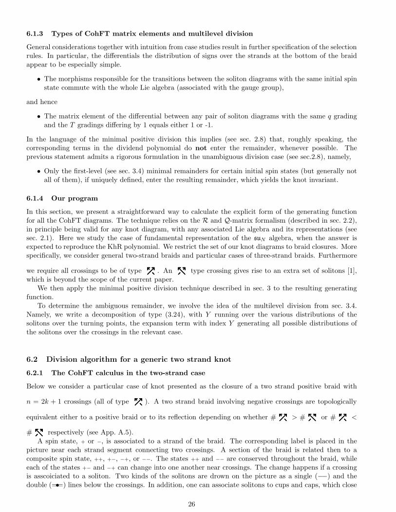
Below we consider a particular case of knot presented as the closure of a two strand positive braid with
n = 2k + 1 crossings (all of type ). A two strand braid involving negative crossings are topologically
equivalent either to a positive braid or to its reflection depending on whether # > # or # <
# respectively (see App. A.5).A spin state, + or −, is associated to a strand of the braid. The corresponding label is placed in the
picture near each strand segment connecting two crossings. A section of the braid is related then to acomposite spin state, ++, +−, −+, or −−. The states ++ and −− are conserved throughout the braid, whileeach of the states +− and −+ can change into one another near crossings. The change happens if a crossingis asscoiciated to a soliton. Two kinds of the solitons are drown on the picture as a single (−−) and thedouble (=•=) lines below the crossings. In addition, one can associate solitons to cups and caps, which close
26

the braid diagram at the top and the bottom ends. The arrangement of the solitons encodes the initial spinstate of the system. All four possible arrangements are illustrated in (6.1), where soliton carrying cups andcaps with like ∪− and ∩−, respectively. The obtained picture is called in [1] a soliton diagram.
We represent a soliton diagram as a word, where each of n letters indicates what happens at the corre-sponding crossing. Namely, × stands for the lack of soliton, while | and ↑↑• stand for the solitons of thetwo kinds (following [2], with put the arrows showing the transport of the spin state). We word put theword in the square brackets and write the initial spin states in front of them. The spin states in all otherbraid sections can be successively obtained as one knows if there is a soliton at each crossing. The final spinstate of the system must coincide with the initial one.
The examples of the soliton diagrams together with the corresponding words are given in table (6.1).
++
++
++
[|]
s
+
−
+
+
−
+
−
−
s
−
+
+
+
+
−
+
−
−
−
−
+
−−
−−
−−
[|]
+−
[× × ↑↑•
]−+
[× ↑ ↑↑• ↑
]
(6.1)
Below we enumerate the soliton diagrams with help of the corresponding words, treating the latter onesas products of non-commutative variables (the letters) and construct explicitly the generating function forall the allowed words.
Then we search for an algorithm of presenting the generating function as (3.6)-type decomposition withthe desired knot invariant as a remainder. For that we apply the “multi-level” division trick from sec. 3.4with Y ∈
{++,−−,+−,−+
}.
We find that
• The first-level remainders are unambiguous (see sec. 3.2) for any number or crossings.
• The second-level division can be performed algorithmically, by operating with the introduced non-commutative variables according to certain “reduction rules”.
The corresponding “reduction rules” are explicitly formulated below, in ssec. 6.2.2, 6.2.3.
6.2.2 Khovanov (N = 2) case
1. Calculate
P2,n(q, T ) = Rn=ξ= +Tr
{
Rn±
(ξ±
ξ∓
)}
(6.2)
with
R= =(q), R± =
(q TT q + Tq−1
)
. (6.3)
2. Expand
P(ξ|q, T ) =∑
Y
PY (q, T )ξY , Y ∈ {++,−−,+−,−+}. (6.4)
27

3. Perform the first-level reduction
PY (q, T ) =∑
k
qkϑ=ϑmax
Y,k∑
ϑ=ϑminY,k
CYϑ,uT
ϑ → PY
I(q, T ) ≡
∑
k
qkT ϑminY,k . (6.5)
4. Perform the second-level reduction
1. qξ+ + q−1Tξ± → 0.2. T 2k+1ξ± + T 2k+2ξ∓ → 0.
(6.6)
Do not reduce T 2kξ± + T 2k+1ξ∓ → 0 !
5. Substitute ξ+ = q2, ξ− = q−2, ξ± = ξ∓ = 1 .
6. The KhR polynomial equals
Kh[2,n](q, T ) = q−2nPII(q, T ) . (6.7)
For each particular odd n the result reproduces the Khovanov polynomial for the two-strand knot withn crossings (torus knot T [2, n]) [7]. The particular case n = 5 is explicitly worked out below. Even ncorrespond to links, which we do not consider here.
6.2.3 KhR for generic N
1. Take the expansion (6.4), reduced as in item 2 of sec. 6.2.2,
PI(q, T ) =
∑
Y
PY
I(q, T )ξY =
∑
Y
ξY∑
k
qkT ϑminY,k . (6.8)
2. Substitute whenever possible
1. qnξ= + qn−2Tξ< → qN+n−1[N ].2. q2T 2k+1ξ< + q−2T 2k+2ξ> → T 2k+1
(qN + Tq−N
)[N − 1].
(6.9)
3. The KhR polynomial of the torus knot T [2, n] equals
KhR[2,n]N (q, T ) = q−nN P
II(N |q, T ) . (6.10)
The result coincides with formula (4.55) from [3] (earlier proposed in [24] for the superpolynomials).
KhR[2,n]N (q, T ) = q−(n−1)(N−1)
[N ] + [N − 1](1 + q−2T
)2j≤n∑
j=0
qn−2j−4T 2j
. (6.11)
6.2.4 Primary polynomials as “deformed” HOMFLY polynomials
Expression (6.2) is the result of deformation (2.23) of the R-matrix representation for the HOMFLY invari-ant (2.4), applied to the particular case of a two-strand braid closure [36, 3]. Namely,
P[2,n] = Qin+1
i1Qjn+1
j1
∏
k=1n
Rikjkjk+1ik+1
=N∑
i=1
(QiiQ
iiR
iiii
)n+
N∑
i<j=1
(
QiiQ
jj(R
N± )ijij +Qj
jQii(R
N± )jiji
)
, (6.12)
28

where
R= = Riiii =
ii
q ii , 1 ≤ i ≤ N, R± =
(
Rijij R
jiij
Rijji R
jiji
)
∼=(
ij ji
0 T ijT q + Tq−1 ji
)
, 1 ≤ i < j ≤ N. (6.13)
Note thatR± is obtained from the block of the “deformed”R-matrices (2.11) by cancelling the q(1+T ) entry.Since the blocks (6.13) of the R-matrix are independent of i and j, Q enters (6.12) only in combinations
ξ= =N∑
i=1
(Qii
)2, ξ± =
N∑
i<j=1
QiiQ
jj , ξ∓ =
N∑
j<i=1
QjjQ
ii. (6.14)
If one considers Qii as (generically non-commutative) operators, this yields (6.2). All the ξ’s must then be
treated as formal operators, independent of each other, as well as of q and T , until all the reduction stepsare performed.
The factors in (6.7, 6.10) are the particular cases of the framing factors (skipped in (2.4), but nowrestored; see App. A.3, where we should set w = n, and N = 2 to get (6.10)).
The substitutions in item 2 of sec. 6.2.3 are motivated by the identities for the corresponding terms inthe HOMFLY polynomial, respectively,
qξ= + q−1Tξ< HOMFLY✛ ✲ q [2N ][2] − q−1 [N ][N−1]
[2] = q[N ]2 − [N ][N − 1] = qN [N ]
‖
[N ]2 − [N ][N−1][2]
, (6.15)
and
q2ξ> + q−2Tξ< HOMFLY✛ ✲(q2 − q−2
) [N ][N − 1]
[2]=(q − q−1
)[N ][N − 1] =
(qN − q−N
)[N − 1]. (6.16)
6.2.5 Comparing the N = 2 and N > 2 cases
The reduction rules: N = 2 as a particular case of generic N . The level II reduction rules lookdifferently for N = 2 (sec. 6.2.2, item 4) and for generic N (sec. 6.2.3, item 2). Here we comment on theirrelationship.
The first of the N = 2 rules, written in schematic form
qnξ= + qn−2Tξ± → qn−1[2], (6.17)
with ξ= ≡ ξ+ + ξ−, just takes the form of the general rule, with N = 2 substituted.The case of the second rule is different. Namely, the N = 2 rule (item 4 from sec. 6.2.2) is manifestly
asymmetric between the odd and even T powers (see the comment in the boldface), while the general N rule(item 3 from sec.6.2.3) appear to be symmetric. In fact, there are several versions of the reduction rule forN ≥ 3, all yielding the same remainder. In particular, one can take a straightforward generalization of theN = 2 rule, which is illustrated in Tab. 6.18, 6.19.II for the N = 2 and N = 3 cases. One should comparethis with the rule in Tab. 6.19.I, which we adhere to, and one more possibility in Tab. 6.19.III.
N = 2 min(i, j)
max(i, j) 0
1 q · q−1 ×
q−1T 3 + q−1T 4 →/ 0 ;qT 2 + qT 3 → 0, q−1T 4 + q−3T 5 → 0.
❅❅❘qT2 q−1T 3
✟✟✟✟✯q−3T 4 q−5T 5 i < j
q3T 2 ❅❅❘qT3 q−1T 4
✟✟✟✟✯q−3T 5 i > j
(6.18)
29

N = 3 min(i, j)
max(i, j) 1 0
2 q2 · 1 q2 · q−2
1 1 · q−2×
qT 2 q−1T 3 i < jq3T 2 qT 3 i > j
Iq[2]T 2
(q + q−1T
)[3] → qT 2[2]
(q[2](q3 + q−3T
)
qT 2 ×
(
q2 �✒1
�✠q−2
)
q−1T 3 ×
(
��✒q2
�✠1
q−2
)
q3T 2 ×
(
q2 ❅❘1
❅■q−2
)
qT 3 ×
(
❅❘q2 ❅■1
q−2
)
(6.19)
IIq2T 2(q + q−1T )[3] → qT 2(q2 + q−2T )[2]
qT 2(1 + T )[3] → 0
❅❅❘qT2 ×
(q2 1
q−2
)
q−1T 3 ×
❅■q
2 1
q−2
q3T 2 ×
(
q2 1
❅■q−2
)
❅❅❘qT3 ×
(q2 1
q−2
)
III
qT 2 ×
(
❅❘q2 �✒1
❅■q−2
)
q−1T 3 ×
��✒q2 1
q−2
q3T 2 ×
(
q2 1
�✠q−2
)
qT 3 ×
(
❅❘q2
�✠1
❅■q−2
)
In particular, one can see from the tables (6.19) that the odd-even asymmetry in fact is present in allversions of the reduction rules. However, the resulting remainder does not include a ∼ (1 + T ) contributionin case N ≥ 3. The difference is due to the additional q-power factors (arranged below in the trianglematrices), which account for various initial states giving rise to the same set of the soliton diagrams. Hence,
• The KhR polynomial of a two-stand knot is a minimal remainder for N ≥ 3, unlike the Khovanovpolynomial (N = 2) of the same knot.
To summarize,
• The N = 2 reduction rules are a particular case of the generic N reduction rules,
in the considered case of the two-strand knots. However, this is not so for a general knot becausenaive substitution of N = 2 in the (large N) KhR polynomial does not always yield the correct Khovanovpolynomial (compare the explicit examples in [22] with that in [7], and see e.g., in [3] for discussion).
Now we return to the N = 2 (Khvanov) case, which provides enough illustrations to the following discussion.
6.2.6 The primary polynomial as the generating function for the soliton diagrams
Diagram rules (A.33) from [1] can be written in the matrix notations as
P → P : R= → R= =(
|), R± → R± =
(
0 ×× ↑ + ↑↑•
)
, (6.20)
(one must substitute q → qT , [0] → 1, [f0] → 1, [f0+1] → T in (A.33) and extract the common factor q−1
2 toobtain our formulas). The primary polynomial (6.2) subjected to further “deformation” (6.20) thus becomesthe generating function for the soliton diagrams from [1]. If we put N = 2 and i, j ∈ {+,−} in (6.12) (amore detailed version of (6.2)), then the upper and the lower pair or indices of each R corresponds tothe composite spin state below and above the corresponding crossing, respectively. The braids with thecomposite spin state ++ and −− in the first (and hence in any other) section are enumerated by the diagonalterms entering with the coefficient ξ=, and all such diagrams yield the same “amplitude” Rn
=. In turn, thebraids with composite spin states +− or −+ in each section are enumerated by the off-diagonal terms. Thesestates can exchange in each crossing in the way encoded in the 2 matrix R± in (6.20), so that all possiblesoliton diagrams are enumerated by the expansion of the trace in (6.2), where the diagram with the initialspin state +− or −+ enters with the coefficient ξ± or ξ∓, respectively.
30

Combinatorial expressions for the numbers of the soliton diagrams. The number of the solitondiagrams with initial spin state ± or ∓ can as well be explicitly computed from combinatorial considerations,respectively,
♯{+−
[(××c ↑
w ↑↑•b)]}
=(w + b+ c)!
w! b! c!, w + b+ 2c = n, (6.21)
and
♯{−+
[×(××c ↑
w ↑↑•b)×]}
=(w + b+ c)!
w! b! c!, w + b+ 2c = n− 2, (6.22)
where the notations in the l.h.s. imply that we count distinct configurations obtained by the variouspermutations of w letters | , b letters ↑↑• , and c letters ×× in the parentheses. Denied that numbers (6.21)
and (6.22) are polynomial coefficients in the expansion of (x+ y + z)w+b+c, the proper generating functions
f±n (x, y, z) =
∑
w+b+2c=n
(w + b+ c)!
w! b! c!xwybz2c = Φn1,1, (6.23)
f∓n (x, y, z) = f±
n−2(x, y, z) = Φn2,2,
are expressed for generic n either as elements of powers of the matrix
Φ =
(0 cc w + b
)
, (6.24)
or as rational functions of its eigenvalues
λ1,2 =1
2
(
w + b±√
(b+ w)2 + 4c2)
. (6.25)
These functions becomes the polynomials only if one substitutes the particular integer for n.For the initial spin states −− and ++ one gets trivially
♯{++
[(|n)]}
= ♯{−−
[(|n)]}
= 1 (6.26)
with the generating function f=n (x) = 2xn.
(6.27)
Primary polynomial (6.2, 6.3) is then obtained from the entire generating function
fn(x, y, z) = ξ=fn=(x, y, z) + ξ±f
n±(x, y, z) + ξmpf
n∓(x, y, z) (6.28)
as the result of the substitution
P2,n(ξ, q, T ) = fn(q, q−1T, T ). (6.29)
Employing the selection rules for the matrix elements in the division procedure. Deformationrule (6.20) sets a one-to-one correspondence between the monomials in primary polynomial (6.2) and thesoliton diagrams. Then,
• The pairs of terms to delete in the reduction rules of sec. 6.2.2 correspond to the pairs of solitondiagrams of [1] between which the transition is allowed20.
20In fact, the allowed transitions in [1] are related to a slightly different reduction rules, yet producing the same answer (seethe explicit example below)
31

+ − +
+ − −
+ − −
− + +
[↑ ×
|
]
Figure 4: A piece of athree strand braid B =(. . . , 1, 2, 1, . . .), with apossible distribution ofthe spin states (+ and−) on the stands, andof the solitons in thecrossings. On the rightis our notation for theobtained diagram.
Covariance under cyclic permutations. The suggested reduction rules arenot invariant, but rather covariant under the equivalence transformations of theknot diagram, namely under the cyclic shift of the crossings (this is the onlytransformation relevant for two-strand braids [6]).
The table below illustrates the behaviour of the various soliton diagrams underthe cyclic shift for two-strand braid with n = 3 crossings (the closure is the trefoilknot, 31 in [7]). Each diagram in the leftmost column is mapped to itself. Thediagrams arranged in triangles are mapped into each other along the arrows. Thecancellation of the diagrams arranged in the vertical pairs obeys the local rule(↑ ↑↑• )+ (××) ∼ 0 (see [1]) for detailed discussion of this rule in particular cases).
++
[|||]
−−
[|||]
+−
[↑ ↑ ↑
]
+−
[↑↑• ↑↑• ↑↑•
]
+−
[↑ ↑ ↑↑•
]
−+
[× ↑×
]
��✠ ❅
❅■
+−
[↑ ↑↑• ↑
]
+−
[↑××
]✲
+−
[↑↑• ↑ ↑
]
+−
[×× ↑
]
+−
[↑↑• ↑↑• ↑
]
−+
[× ↑↑• ×
]
��✠ ❅
❅■
+−
[↑↑• ↑ ↑↑•
]
+−
[↑↑• ××
]✲
+−
[↑ ↑↑• ↑↑•
]
+−
[×× ↑↑•
]
(6.30)
6.2.7 Example: torus knot T 2,5.
The simplest example, when all the above features are non-trivial, is presented inTab. 5. Nothing essentially new happens for a two-stand knot with an arbitrarynumber of crossings.
The contributions to the first-level remainder are boxed. The contributionsto the second-level remainder are double boxed. The terms marked by the same Roman numerals (upper-case) “cancel each other” under the second level reduction. The lowercase labels mark the pairs of terms“cancelling” in the [1] version of the reduction instead. The resulting remainders in the two cases containdifferent sets of the soliton diagrams but are equal as polynomials in q and T , both yielding the correctvalue of the Khovanov polynomial for T [2, 5] knot (51 in [7]).
6.3 The first-level division for particular three-strand knots
Now we turn to the first attempt to treat a more general case using our approach which is the hybridbetween the CohFT calculus and positive division technique.
Below we restrict our considerations to the case of Khovanov polynomials (N = 2), which already appearto be rather involved.
6.3.1 A draft of the three-strand reduction procedure
The list below almost literally follows the two-stand algorithm, yet differing at each step, with the moststeps not being completely worked out at the moment.
1. For a three-strand braid B =(Bi)n
i=1, Bi = 1, 2 (fig. 4),
PB(q, T ) =∑
Y
TrQY(q)n∏
i=1
RYBi(q, T ), Y ∈
{(000), (001), (011), (111)
}. (6.31)
with
Q(000) =(ξ000
), Q(001) = diag
(ξ001 ξ010 ξ100
), Q(011) = diag
(ξ011 ξ101 ξ110
), Q(111) =
(ξ111
), (6.32)
RY−Bi
(q, T ) = RYBi(q−1, T ), and RY
Bi(q, T ) for Bi > 0 given by (6.36).
32

Table 5: Torus knot [2, 5]. Soliton diagrams associated with all the terms of the primary polynomial, in thefirst-level remainders (boxed), and in the Khovanov polynomial (double boxed).
++
[5 |
]
q5
1
−−
[5 |
]
q5
1
I, i
+−
[(5 ↑
)]
[( ↑ 4 ↑↑•
)]
[(2 ↑ 3 ↑↑•
)]
[(3 ↑ 2 ↑↑•
)]
[( ↑ 4 ↑↑•
)]
[(5 ↑↑•
)]
1 5 = 5!1!4! 10 = 5!
2!3! 10 5 1
q5 q3T qT 2 q−1T 3 q−3T 4 q−5T 5
‖ ‖ ‖ ‖ ‖ ‖
q5 q4(q−1T
)q3(q−1T
)2= q2
(q−1T
)5q(q−1T
)4 (q−1T
)5
I, i II ii III iii[(3 ↑ ××
)]
[(2 ↑ ↑↑• ××
)]
[( ↑ 2 ↑↑• ××
)]
[(3 ↑↑• ××
)]
4 12 = 3!1!2!
(3+1)!3!1! 12 4
q3T 2 qT 3 q−1T 4 q−3T 5
‖ ‖ ‖ ‖
q3 · T 2 q2(q−1T
)· T 2 q
(q−1T
)2· T 2
(q−1T
)3· T 2
[( ↑ 2××
)]
[( ↑↑• 2××
)]
3 = (2+1)!2!1! 3
⋆ qT 4 ⋆ q−1T 5
‖ ‖q · T 2 · T 2
(q−1T
)· T 2 · T 2
−+[× (3 ↑ )×
] [× (2 ↑ ↑↑• )×
] [× (↑ 2 ↑↑• )×
] [× (3 ↑↑• )×
]
1 3 = 3!1!2! 3 1
q3T 2 qT 3 q−1T 4 q−3T 5
‖ ‖ ‖ ‖
T · q3 · T T · q2(q−1T
)· T T · q
(q−1T
)2· T T ·
(q−1T
)3· T
ii II iii III[× (↑ )×××
] [× (↑↑• ××)×
]
2 2qT 4 q−1T 5
‖ ‖T · q · T 2 · T T ·
(q−1T
)· T 2 · T
33

2. Expand
P(ξ|q, T ) =∑
Y
PY(q, T ) ξY , Y ∈{(000), (001), (011), (111)
}. (6.33)
3. I. Reduce
PY (q, T ) = (1 + T )J Y (q, T ) + PYmin(q, T ) → PY
min(q, T ), (6.34)
to the residue containing the minimal possible number of q and T powers, if it is unique.
4. II. Reduce further∑
QY PYmin(q, T ) → ? (6.35)
5. Substitute ξ000 = q3, ξ001 = ξ010 = ξ100 = q, ξ011 = ξ101 = ξ110 = q−1, ξ111 = q−3.
6. The result must be proportional the the Khovanov polynomial of the knot K = B that is the closureof the braid B (the proportionality factor is q−2w with w =
∑Ni=1 Bi, see sec. 6.2.4).
6.3.2 Explicit formulas for the three-strand (deformed) R-matrices
From now on we switch to the notations + → 0 and − → 1, more natural for the R-matrix formalism(especially when aiming for the general N case). Just as in the two-strand case, we omit all the q(1 + T )entries in the R-matrices (as the sources of ∼ (1 + T ) contributions never enter the minimal remainders).All the needed matrices are explicitly given in the table below.
I II IIITo compute HOMFLY polynomial Primary polynomial Generating function
Y k RYk RY
k RYk
(000),(111)
1,2
(
iii
q iii) , i = 0, 1(q) (
|)
(001) 1
(
001 010 100
q 001q − q−1 −1 010−1 100
)
qq + q−1T T
T
|
↑ + ↑↑• ××
2
(
001 010 100
q − q−1 −1 001−1 010
q 100
)
q + q−1T TT
q
| + ↑↑• ××
|
(011) 1
011 101 110
q − q−1 −1 101−1 101
q 110
q + q−1T TT
q
| + ↑↑• ××
|
2
(
011 101 110
q 011q − q−1 −1 101−1 110
)
qq + q−1T T
T
|
| + ↑↑• ××
(6.36)
34
6.4 The generating function for the three-strand soliton diagrams
Similarly to the two-strand case, expression (6.31) for the three-strand primary polynomial turns into agenerating function for the soliton diagrams associated with the braid B, if one substitutes R from col. IIIinstead of R from from col. II of (6.36), each monomial in the primary polynomial being then related to acertain soliton diagram.
We consider only the positive braids, i.e., all the crossings being the type, and respectively allBi > 0. The form of a three strand braid is much more constrained by such assumption, than the form of atwo strand braid (see sec. 6.2).
6.4.1 Guide to the experimental data
The three-strand positive braids with no more than 8 crossings, together with the knots or links being theirclosures, are enumerated in App. D. Examples of the unique remainders, with each term related to a set ofsoliton diagrams, are given in App. E:
1. for the doubly twisted unknot diagram, presented as three-strand braid with 2 crossings (App. E.1),
2. for all possible diagrams of the trefoil knot having form of three-strand braids with 4 crossings andproviding the unique first level remainders (App. E.2)
3. for torus knot T [3, 4] (819 in [7]), presented as a three-strand braid with 8 crossings 21.
7 Further directions
We complete our presentation by enumerating the most natural directions for the following research.
1. Systematic study of the m ≥ 3 strand case. Of course, the attempt presented in sec. 6.3 is justthe first and a very naive one.
2. Relation to the standard Khovanov-Rozansky construction. It is mysterious that the KhRconstruction, apparently following just one of several possible options at many points of the procedure(in particular, see the footnotes in the beginning of sec. 2.4 and in the beginning of 2.6), is discussedin the mathematical literature only in its original literal formulation [4, 22] ??? N = 3 ???. Anyalternative (even not essentially different mathematically), if found, can be useful for various applica-tions. A detailed comparison of the R-matrix construction, schematically described in sec. 2 and insec. 4, with the rigorously formulated KhR construction, both on the general level and with explicitexamples, provides some advances in this direction.
3. Relation to the differential expansion. This issue touched in sec. 5 definitely deserves a systematictreatment.
4. The problem of finite N . The problem is in particular discussed in [3] and mentioned in sec. 6.2.5.The definition of the KhR polynomial [4] initially refers to the same notions, as the R-matrix definitionof the HOMFLY polynomial, until the differentials are introduced. In particular, both invariants areassociated with the suN series of the Lie algebras (we tried to present this point mostly explicit insec. 2). However, the HOMFLY invariants admit the most naive analytical continuation to arbitrarycomplex value of N , while the KhR polynomials admits one only for N ≤ N0 (with N0 depending onthe knot). The “phase transition” at N = N0, which definitely happens at the level of homologies, isstill not well studied and attracts a lot of attention.
21This case deserves special interest, as the simplest case of the “thick” knot, i.e., when the Khovanov polynomial is not
recovered by setting N = 2 in the KhR polynomial [3].
35

5. Higher representations and other groups. Finally, the R-matrix based approach possesses ahighly inspiring property, already mentioned in sec. 2. Namely, in principle it can be extended toarbitrary Lie groups and representations, on the ground of the already exiting R-matrix approachesto other knot invariants [6]. The coloured (related to higher representations of the suN Lie algebra)analogs of the KhR invariants are widely studied in various (often semi-empiric) ways [24, 25, 27, 28,31, 9] (the list of references can be expanded). Yet the subject is even further from being exhausted,than the case of ordinary KhR invariants. In particular, even exact definition of the coloured KhRinvariants (superpolynomials) faces essential difficulties, in particular, discussed in [30, 32] (the secondpaper concerns a possible extension of the cabling approach [44] to the superpolynomials).
6. Can one use the CohFT calculus as a tool in the KhR calculus? This is the most intriguingpoint of the story. In fact, this work was originally motivated by this question. Authors of [1, 2] followthe CohFT logic and associate the knot polynomials with the partition function for BPS states. Theyconsider the resolutions of the knot diagram (representing the basis vectors in the complex) as thesoliton states in the CohFT, and they relate the action of the differentials to the instantons responsiblefor the soliton scattering. They also discuss the wall-crossing phenomenon in this context. Yet, alltheir considerations remain rather a matter of art, than a regular technique. It is still unclear, whetherthe such technique can at all be developed in the CohFT framework.
Acknowledgements
The author is deeply indebted to A. Yu. Morozov for scientific direction of this work, and to D. Galakhovand I. Danilenko for long inspiring discussions and patient explanations. The author truly appreciates thegreat work of Ye. Zenkevich, who careffully read the draft and helped to prepare it for publishing, andalso the work of G. Aminov, who helped to correct the appendices. The author thanks S. Arthamonov,And. Morozov and A. Popolitov for the valuable comments, and M. Bishler, D. Vasiliev, Ya. Kononov,S. Mironov, N. Nemkov, A. Sleptsov together with all other participants of the Mathematical physics groupseminar for interest to this work.
The author is also grateful to the secretary of the mathematical physics group E. S. Syslova, who makesthe work of the author and his colleagues possible for many years.
This work was funded by the Russian Science Foundation (grant N 16-12-10344).
References
[1] Galakhov D., Moore G. –– arXiv : hep-th/1607.04222.
[2] Galakhov D. –– arXiv : hep-th/1702.07086.
[3] Anokhina A., Morozov A. // JHEP. –– 2014. –– Vol. 07, no. 063. –– arXiv : hep-th/1403.8087.
[4] Khovanov M., Rozansky L. Matrix factorizations and link homology // Fund. Math. –– 2008. –– Vol.199. –– P. 1–91. –– arXiv : math.QA/0401268.
[5] Khovanov M. A categorification of the Jones polynomial // Duke Math. J. –– 2000. –– Vol. 101. ––P. 359–426.
[6] Kauffman L. H. The interface of knots and physics. –– Singapore : World Scientific, 2001. –– P. 788.
[7] Bar-Natan D., Scott M., et al. The Knot Atlas. –– URL: http://katlas.org (online; accessed:22.10.17).
[8] Morozov And., Sleptsov A., et al. The knotebook. –– URL: www.knotebook.org (online; accessed:22.10.17).
36
[9] Gukov Sergei, Khovanov Mikhail, Walcher Johannes. Physics and Mathematics of Link Homology. ––Providence : AMS, 2016. –– P. 177.
[10] Gukov S., Schwarz A., Vafa C. Khovanov-Rozansky homology and topological strings // Lett. Math.Phys. –– 2005. –– Vol. 74. –– P. 53–74. –– arXiv : hep-th/0412243.
[11] Rasmussen Jacob. –– 2006. –– arXiv : math.GT/0607544.
[12] Dunfield N. M., Gukov S., Rasmussen J. The superpolynomial for knot homologies // ExperimentalMath. –– 2006. –– Vol. 15. –– P. 129–159. –– arXiv : math/0505662.
[13] Gorsky Eugene, Lewark Lukas // Experimental Mathematics. –– 2015. –– Vol. 24. –– P. 162–174. ––arXiv : math.GT/1404.0623.
[14] Gaiotto D., Witten E. –– arXiv : hep-th/1106.4789.
[15] Schwarz A. S. New topological invariants arising in the theory of quantized fields // InternationalTopological Conference. –– Vol. 2. –– Baku : Institute of Mathematics and Mechanics of the AzerbaijanAcademy of Sciences of USSR, 1987.
[16] Witten E. Quantum field theory and the Jones polynomial // Comm. Math. Phys. –– 1989. –– Vol.121. –– P. 351–399.
[17] Witten E. Gauge theories and integrable lattice models // Nucl. Phys. –– 1989. –– Vol. B322. –– P. 629–697.
[18] Bar-Natan D. On Khovanov’s categorification of the Jones polynomial // Algebr. Geom. Topol. ––2002. –– Vol. 2. –– P. 337–370. –– arXiv : math.QA/0201043.
[19] Dolotin V., Morozov A. Introduction to Khovanov homologies. I. Unreduced Jones superpolynomial //JHEP. –– 2013. –– Vol. 1301, no. 065. –– arXiv : hep-th/1208.4994.
[20] Dolotin V., Morozov A. Introduction to Khovanov homologies. II. Reduced Jones superpolynomials //J. Phys.: Conf. Ser. –– 2013. –– Vol. 411, no. 012013. –– arXiv : hep-th/1209.5109.
[21] Nawata Satoshi, Oblomkov Alexei. Proceedings of.
[22] Carqueville N., Murfet D. Computing Khovanov-Rozansky homology and defect fusion // Algebr.Geom. Topol. –– 2014. –– Vol. 14. –– P. 489–537. –– arXiv : hep-th/1108.1081.
[23] Dolotin V., Morozov A. Introduction to Khovanov homologies. III. A new and simple tensor-algebraconstruction of khovanov-rozansky invariants // Nucl. Phys. –– 2014. –– Vol. B878. –– P. 12–81. –– arXiv :hep-th/1308.5759.
[24] Superpolynomials for torus knots from evolution induced by cut-and-join operators / P. Dunin-Barkowski, A. Mironov, A. Morozov et al. // JHEP. –– 2013. –– Vol. 03, no. 021. –– arXiv : hep-th/1106.4305.
[25] Mironov A., Morozov A., Morozov An. Evolution method and “differential hierarchy” of colored knotpolynomials // AIP Conf. Proc. –– 2013. –– Vol. 1562. –– arXiv : hep-th/1306.3197.
[26] Evolution method and HOMFLY polynomials for virtual knots / L. Bishler, A. Morozov, And. Morozov,Ant. Morozov // Int. J. of Mod. Phys. –– 2015. –– Vol. A30, no. 1550074. –– arXiv : hep-th/1411.2569.
[27] Gorsky E., Gukov S., Stosic M. Quadruply-graded colored homology of knots. –– 2014. –– arXiv :math.QA/1304.3481.
[28] S.Arthamonov, A.Mironov, A.Morozov // Theor.Math.Phys. –– 2014. –– Vol. 179. –– P. 509–542. ––arXiv : hep-th/1306.5682.
37

[29] Kononov Ya., Morozov A. // JETP Letters. –– 2015. –– Vol. 101. –– P. 831–834. –– arXiv : hep-th/1504.07146.
[30] Khovanov Mikhail // Knot theory and its Ramifications. –– 2005. –– Vol. 14, no. 1. –– P. 111–130. ––arXiv : math.QA/0302060.
[31] Nawata S., Ramadevi P., Zodinmawia // JHEP. –– 2014. –– Vol. 1401, no. 126. –– arXiv : hep-th/1310.2240.
[32] Danilenko I. –– arXiv : hep-th/1405.0884.
[33] Turaev V. G. The Yang-Baxter equation and invariants of links // Invent. Math. –– 1988. –– Vol. 92. ––P. 527–533.
[34] Reshetikhin N. Yu., Turaev V. G. Ribbon graphs and their invariants derived from quantum groups //Commun. Math. Phys. –– 1990. –– Vol. 127. –– P. 1–26.
[35] Morozov A., Smirnov A. Chern-simons theory in the temporal gauge and knot invariants throughthe universal quantum R-matrix // Nucl. Phys. –– 2010. –– Vol. B835. –– P. 284–313. –– arXiv : hep-th/1001.2003.
[36] Mironov A., Morozov A., Morozov And. Character expansion for HOMFLY polynomials. II. fundamen-tal representation. up to five strands in braid // JHEP. –– 2012. –– Vol. 03. –– arXiv : hep-th/1112.2654.
[37] Anokhina A. On R-matrix approaches to knot invariants. –– 2014. –– arXiv : hep-th/1412.8444v2.
[38] Klimyk A., Schmudgen K. Quantum groups and their representations. –– Berlin : Springer, 2012. ––P. 552.
[39] Groups Loop. Andrew Pressley and Graeme Segal. –– Oxford : Clarendon Press, Oxford MathematicalMonographs, 1988. –– P. 316.
[40] S.I. Gelfand, Yu.I. Manin. Homological Algebra. –– Berlin : Springer, 1994. –– P. 222.
[41] G.Fourier, P.Littelmann // Advances in Mathematics. –– 2007. –– Vol. 211, no. 2. –– P. 566–593. ––arXiv : hep-th/1702.07086.
[42] Elias Ben, Hogancamp Matthew. –– 2016. –– arXiv : math.GT/1603.00407.
[43] Hogancamp Matthew. –– 2017. –– arXiv : math.GT/1704.01562.
[44] A.Anokhina, An.Morozov // Theor.Math.Phys. –– 2014. –– Vol. 178. –– P. 1–58. –– arXiv : hep-th/1307.2216.
[45] Sergei Gukov Marko Stosic // Geometry & Topology Monographs. –– 2012. –– Vol. 18. –– P. 309–367. ––arXiv : hep-th/1112.0030.
A Basic properties of the special point operators
A.1 General constraints on the special point operators
A.1.1 Continuous space transformations and transformations of the knot diagram.
The knot K as a curve in the space is considered up to arbitrary continuous space transformations. However,the corresponding transformations of the knot diagram D(K) (see sec. 2) include, apart from arbitrarycontinuous plane transformations, certain singular transformations generated by the Reidemester moves [6].The latter ones are the elementary transformations of the special points on the knot diagram. Two ofthe moves, RII and RIII (fig. A.1), involve only the crossings, and one more move, RI (A.3), involves theturning points as well. In addition, one should consider the transformations generated by the elementarytransformations in fig. A.2, which involve only the turning points on the knot diagram [6].
38

A.1.2 Topological invariance constraints on the crossing and turning point operators.
By definition, contraction (2.4) ignores the continuous, turning point-preserving planar transformations.Hence, the obtained quantity is a topological invariant provided that the operators R and Q satisfy a finiteset of constraints explicitly presented below.
A.2 Constraints on the R-matrices
Transformations in fig. A.1 are the planar projections of the continuous space transformations. Yet theyaffect non-trivially on the knot diagram and can identified with the generators of the vertices changingsubgroup of the entire equivalence transformations group. The corresponding space constraints on thevertex (R) operators are presented below each figure.
i j
a b
k l
=
i j
k l
j
a
i
c
bm
lk
p =
ji
ca
m
l
b
k
p−Rjiab
+Ralkb = δikδ
jl
∗Riajc
∗Rpbcm
∗Rblak =
∗Rpbia
∗Rbljc
∗Rakcm, ∗ ∈ {+,−} .
(A.1)
A.3 Relations between the R and Q-matrices
Extremum point operators. The described approach to the knot invariants also requires for selectinga direction in the plane [34, 6, 35]. As a result, one must treat the turning points as two-valent vertices onthe knot diagram of the four kinds, r ,
r, r , and
r.
The equivalence transformations of the knot diagram that change the number of the turning points mustbe considered separately. These transformations form a finite subgroup, and their generators give rise tothe relations between different Q, as well as between R and Q matrices (both presented below).
r
r ijk∼=
ikr
ri j k∼=
i k
∗Q✠ij
∗Q■jk = δik
∗Q✠ij
∗Q■jk = δik
(A.2)
r
rp
l
i
k
j∼=
r
rp
l
j
k
i∼= i
k
∗Q■jp
∗Q✠pl Rij
kl = ∗Q✠jp
∗Q■plR
ijkl = κδik
(A.3)
The factor κ here depends on the particular solutions of (A.1) for the R operators. In particular, κ = q−N
for solution (2.6).
Framing factor. Multiplied on κw = q−wN , where w ≡ # − # is the algebraic number of
crossings on the knot diagram, contraction (2.4) becomes topologically invariant. One can set κ = 1 byusing homogeneity property of constraints (A.1) to rescale the R → κR. Yet the resulting R explicitlydepends on the chosen Lie algebra suN via N , and this is why we do not make such rescaling here.
39
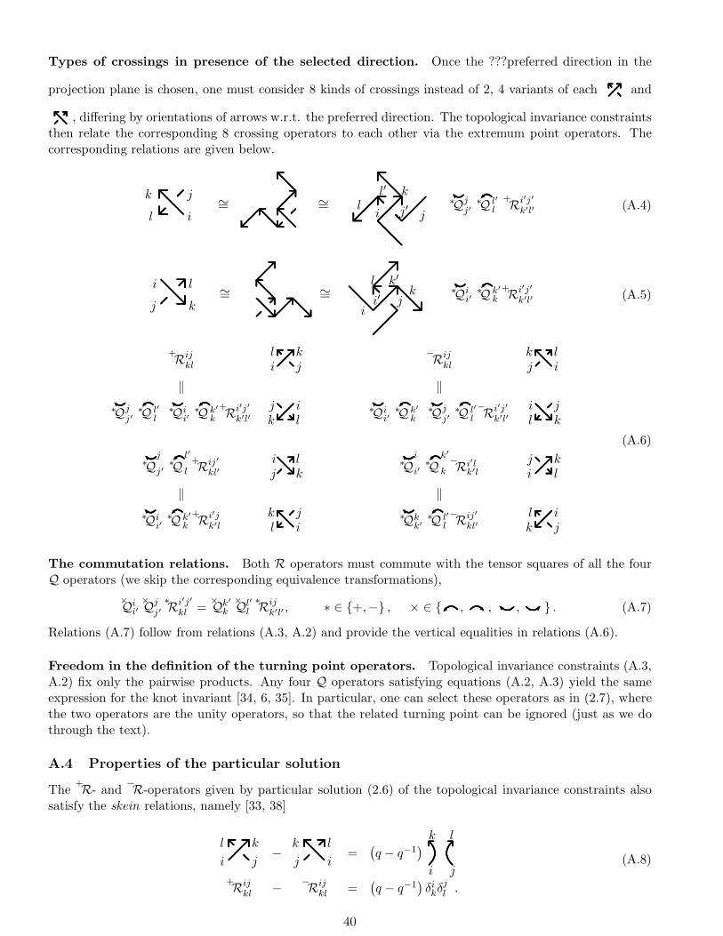
Types of crossings in presence of the selected direction. Once the ???preferred direction in the
projection plane is chosen, one must consider 8 kinds of crossings instead of 2, 4 variants of each and
, differing by orientations of arrows w.r.t. the preferred direction. The topological invariance constraintsthen relate the corresponding 8 crossing operators to each other via the extremum point operators. Thecorresponding relations are given below.
l
k
i
j ∼= ∼=l′
j′il
j
k∗Q■j
j′∗Q✠l′
l
+Ri′j′
k′l′ (A.4)
j
i
k
l ∼= ∼= i′k′
i
l
jk ∗Q■i
i′∗Q✠k′
k
+Ri′j′
k′l′ (A.5)
+Rijkl i
ljk −
Rijkl j
kil
‖ ‖
∗Q■jj′
∗Q✠l′
l∗Q■i
i′∗Q✠k′
k
+Ri′j′
k′l′ kj
li ∗Q■i
i′∗Q✠k′
k∗Q■j
j′∗Q✠l′
l
−Ri′j′
k′l′ li
kj
∗Q■j
j′∗Q✠l′
l
+Rij′
kl′ ji
kl ∗Q■
i
i′∗Q✠k′
k
−Ri′lk′l i
jlk
‖ ‖
∗Q■ii′
∗Q✠k′
k
+Ri′jk′l l
kij ∗Q■k
k′∗Q✠l′
l
−Rij′
kl′ kl
ji
(A.6)
The commutation relations. Both R operators must commute with the tensor squares of all the fourQ operators (we skip the corresponding equivalence transformations),
×Qii′×Qjj′
∗Ri′j′
kl =×Qk′
k
×Ql′
l
∗Rijk′l′ , ∗ ∈ {+,−} , × ∈ {✠ , ❘ , ■ ,
✒} . (A.7)
Relations (A.7) follow from relations (A.3, A.2) and provide the vertical equalities in relations (A.6).
Freedom in the definition of the turning point operators. Topological invariance constraints (A.3,A.2) fix only the pairwise products. Any four Q operators satisfying equations (A.2, A.3) yield the sameexpression for the knot invariant [34, 6, 35]. In particular, one can select these operators as in (2.7), wherethe two operators are the unity operators, so that the related turning point can be ignored (just as we dothrough the text).
A.4 Properties of the particular solution
The+R- and
−R-operators given by particular solution (2.6) of the topological invariance constraints also
satisfy the skein relations, namely [33, 38]
i
l
j
k−
j
k
i
l=
(q − q−1
)
i j
k l
+Rijkl −
−Rijkl =
(q − q−1
)δikδ
jl .
(A.8)
40
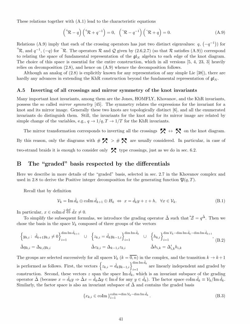
These relations together with (A.1) lead to the characteristic equations
(+R− q
)(+R+ q−1
)
= 0,(−R− q−1
)(−R+ q
)
= 0. (A.9)
Relations (A.9) imply that each of the crossing operators has just two distinct eigenvalues: q,(−q−1
)) for
+R, and q−1, (−q) for
−R. The operators R and Q given by (2.6,2.7) (so that R satisfies (A.9)) correspond
to relating the space of fundamental representation of the glN algebra to each edge of the knot diagram.The choice of this space is essential for the entire construction, which in all versions [5, 4, 23, 3] heavilyrelies on decomposition (2.8), and hence on (A.9) whence the decomposition follows.
Although an analog of (2.8) is explicitly known for any representation of any simple Lie [38]), there arehardly any advances in extending the KhR construction beyond the fundamental representation of glN .
A.5 Inverting of all crossings and mirror symmetry of the knot invariants
Many important knot invariants, among them are the Jones, HOMFLY, Khovanov, and the KhR invariants,possess the so called mirror symmetry [45]. The symmetry relates the expressions for the invariant for aknot and its mirror image. Generally these two knots are topologically distinct [6], and all the enumeratedinvariants do distinguish them. Still, the invariants for the knot and for its mirror image are related bysimple change of the variables, e.g., q → 1/q, T → 1/T for the KhR invariants.
The mirror transformation corresponds to inverting all the crossings ↔ on the knot diagram.
By this reason, only the diagrams with # > # are usually considered. In particular, in case of
two-strand braids it is enough to consider only type crossings, just as we do in sec. 6.2.
B The “graded” basis respected by the differentials
Here we describe in more details of the “graded” basis, selected in sec. 2.7 in the Khovanov complex andused in 2.8 to derive the Positive integer decomposition for the generating function P(q, T ).
Recall that by definition
Vk = Im dk ⊕ coIm dk+1 ⊕Hk ⇔ x = dky + z + h, ∀x ∈ Vk. (B.1)
In particular, x ∈ coIm ddef⇔ dx 6= 0.
To simplify the subsequent formulas, we introduce the grading operator ∆ such that∗Z = q∆. Then we
chose the basis in the space Vk composed of three groups of the vectors
{
yk,i : dk+1yk,i 6= 0}dim Im dk+1
i=1∪
{
zk,i = dkyk−1,i
}dim Im dk
i=1∪{
hk,i
}dimVk−dim Im dk−dim Im dk+1
i=1,
∆yk,i = ∆k,iyk,i ∆zk,i = ∆k−1,izk,i ∆hi,k = ∆′i,khi,k
(B.2)
The groups are selected successively for all spaces Vk (k = 0, n) in the complex, and the transition k → k+1
is performed as follows. First, the vectors{
zk,i = dkyk−1,i
}dim Im dk
i=1are linearly independent and graded by
construction. Second, these vectors z span the space Im dk, which is an invariant subspace of the gradingoperator ∆ (because x = dky ⇒ ∆x = dk∆y ∈ Im d for any y ∈ dk). The factor space coIm dk ≡ Vk/Im dk.Similarly, the factor space is also an invariant subspace of ∆ and contains the graded basis
{xk,i ∈ coIm }coIm=dimVk−dim Im dki=1 . (B.3)
41
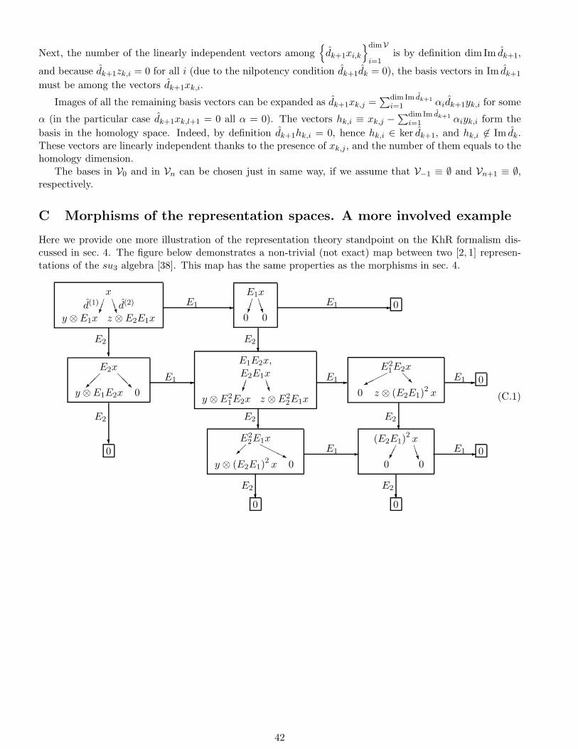
Next, the number of the linearly independent vectors among{
dk+1xi,k
}dimV
i=1is by definition dim Im dk+1,
and because dk+1zk,i = 0 for all i (due to the nilpotency condition dk+1dk = 0), the basis vectors in Im dk+1
must be among the vectors dk+1xk,i.
Images of all the remaining basis vectors can be expanded as dk+1xk,j =∑dim Im dk+1
i=1 αidk+1yk,i for some
α (in the particular case dk+1xk,l+1 = 0 all α = 0). The vectors hk,i ≡ xk,j −∑dim Im dk+1
i=1 αiyk,i form the
basis in the homology space. Indeed, by definition dk+1hk,i = 0, hence hk,i ∈ ker dk+1, and hk,i 6∈ Im dk.These vectors are linearly independent thanks to the presence of xk,j, and the number of them equals to thehomology dimension.
The bases in V0 and in Vn can be chosen just in same way, if we assume that V−1 ≡ ∅ and Vn+1 ≡ ∅,respectively.
C Morphisms of the representation spaces. A more involved example
Here we provide one more illustration of the representation theory standpoint on the KhR formalism dis-cussed in sec. 4. The figure below demonstrates a non-trivial (not exact) map between two [2, 1] represen-tations of the su3 algebra [38]. This map has the same properties as the morphisms in sec. 4.
x
d(1) ✂✂✌ ❇❇◆ d(2)
y ⊗ E1x z ⊗ E2E1x
E1 ✲E1x✂✂✌ ❇❇◆
0 0
E1 ✲ 0
E2
❄
E2❄
E2x��✠ ❅❅❘
y ⊗ E1E2x 0
E1 ✲
E1E2x,E2E1x✂✂✌ ❇❇◆
y ⊗ E21E2x z ⊗ E2
2E1x
E1✲E2
1E2x✟✟✟✙ ❅❘
0 z ⊗ (E2E1)2 x
E1✲ 0
E2
❄
E2❄
E2❄
0
E22E1x
�✠ ❍❍❍❥y ⊗ (E2E1)
2 x 0
E1 ✲(E2E1)
2 x✁✁☛ ❇❇◆
0 0
E1✲ 0
E2❄
E2❄
0 0
(C.1)
42

D List of braids providing the unique level I reminders
The first-level minimal positive integer divition of the primary polynomial, the type
Uniquely determined Ambigious
01 ∪ 01, the pair of unlinked Unknots
[1], [2].
01, the Unknot,Torus [2, 1]
[21], [12].
01 ∪ 211, the Hopf link unlinked with the Unknot
[22], [11].
211, the Hopf link,Torus [2, 2]
[221], [122], [121], [112], [211], [212].
01 ∪ 31, the Trefoil knot as Tourus [2, 3] unlinked with the Unknot
[222], [111].
31, the Trefoil knot, as Torus [3, 2]
[1211], [2221], [2122], [1222], [1112], [1212], [2121], [2212], [2111], [1121].
421, L4a1(1), the Solomon link,Torus [2, 4]
[22122], [21222], [21211], [22121], [12111], [12112], [11212], [12122], [11121], [22212],[21221], [12212], [11211], [21212], [12121], [21121].
[22221], [21111], [12222], [11112].
51, the Fivefoil knot,Torus [2, 5]
[121122], [121211], [222212], [212111], [212122], [121111], [111212], [222122], [122121],[212222], [211212], [212211], [212112], [112122], [121112], [122112], [212221], [121221],[221222], [122212], [112121], [211221], [121222], [221121], [111211], [221212], [222121],[211121], [112212], [111121], [221211], [112111].
[222221], [122222], [111112], [211111].
633, L6n1(0, 1),Torus [3, 3]
[211211], [221221], [121121], [121212], [212121], [122122], [212212], [112112].
727, L7n1(0)
[1221212], [1221221], [1211121], [2122121], [1121112], [2211221], [2121221], [1212112],[1112112], [2121121], [2122122], [1222122], [1221222], [2121212], [1121212], [2112111],[2212221], [2121211], [2112121], [2111211], [2122212], [1122112], [2112112], [1212122],[1221122], [2112211], [1212121], [1212212], [2212121], [2221221], [1211212], [2212212],[1121121], [1211211].
[2211211], [1121122], [2212211], [1221121], [1122122], [1211221], [2112212], [2122112].
819,Torus [3, 4], the first “thick” knot
[12212212], [21211211], [11121122], [21221221], [22122121], [22212211], [21121211],[21121121], [11221222], [12112112], [21212121], [11212122], [12122122], [12212122],[22112111], [22121211], [11212112], [11211212], [22121221], [12121212].
[12112211], [21221122], [22211221], [12211212], [11221112], [11211121], [12112121],[21121112], [12121121], [22112221], [22122212], [11222122], [21122111], [21122212],[12121122], [12111221], [22112121], [12111211], [21211221], [21112111], [12211121],[11121112], [21222122], [21212212], [12122112], [21122122], [21112112], [21112211],[12221222], [11221121], [21212211], [21221212], [11211221], [22212221], [11211122],[11122112], [22122112], [12221122], [21122121], [12212121], [12212221], [21121212],[12112212], [22111211], [11221212], [22112212], [12211211], [21221121], [21222112],[12221221], [21212112], [12211222], [22122211], [12121221].
43
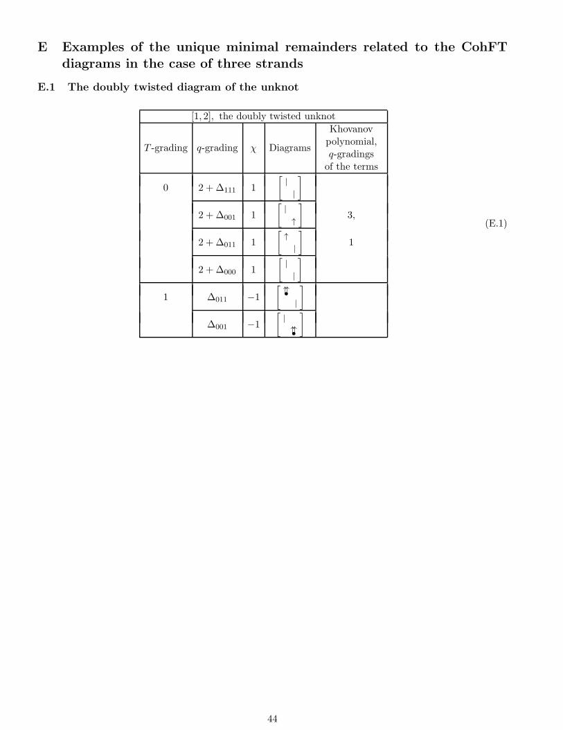
E Examples of the unique minimal remainders related to the CohFT
diagrams in the case of three strands
E.1 The doubly twisted diagram of the unknot
[1, 2], the doubly twisted unknot
T -grading q-grading χ Diagrams
Khovanovpolynomial,q-gradingsof the terms
0 2 + ∆111 1
[|
|
]
2 + ∆001 1
[|
↑
]
3,
2 + ∆011 1
[↑
|
]
1
2 + ∆000 1
[|
|
]
1 ∆011 −1
[↑↑•
|
]
∆001 −1
[|
↑↑•
]
(E.1)
44

E.2 The trefoil knot in different three strand presentations
1. [1112], the Trefoil knot
T -grading q-grading |χ| Diagrams
Khovanovpolynomial,q-gradingsof the terms
0 4 + ∆111 1
[| | |
|
]
4 + ∆000 1
[| | |
|
]
−1,
4 + ∆001 1
[| | |
↑
]
−3
4 + ∆011 1
[↑ ↑ ↑
|
]
1 2 + ∆011 1
[↑↑• ↑ ↑
|
]
,
[↑ ↑↑• ↑
|
]
,
[↑ ↑ ↑↑•
|
]
2 + ∆001 1
[| | |
↑↑•
]
2 2 + ∆100 1
[× ↑×
|
]
2 + ∆101 1
[× ↑×
↑
]
−5
∆011 1
[↑↑• ↑↑• ↑
|
]
,
[↑↑• ↑ ↑↑•
|
]
,
[↑ ↑↑• ↑↑•
|
]
3 2 + ∆011 1
[↑↑• ↑↑• ↑↑•
|
]
∆101 2
[× ↑↑• ×
↑
]
,
[× ↑×
↑↑•
]
−9
∆100 1
[× ↑↑• ×
|
]
4 2 + ∆101 1
[× ↑↑• ×
↑↑•
]
2. [1121], the Trefoil knot
T -grading q-grading |χ| Diagrams
Khovanovpolynomial,q-gradingsof the terms
0 4 + ∆111 1
[| | |
|
]
4 + ∆000 1
[| | |
|
]
−1,
4 + ∆011 1
[↑ ↑ ↑
|
]
−3
4 + ∆001 1
[| | |
↑
]
1 2 + ∆001 1
[| | |
↑↑•
]
2 + ∆011 1
[↑↑• ↑ ↑
|
]
,
[↑ ↑↑• ↑
|
]
,
[↑ ↑ ↑↑•
|
]
2 2 + ∆101 1
[× ↑ ×
|
]
−5
2 + ∆010 1
[↑× ×
|
]
3 ∆101 1
[× ↑↑• ×
|
]
−9
∆010 1
[↑↑• × ×
|
]
45
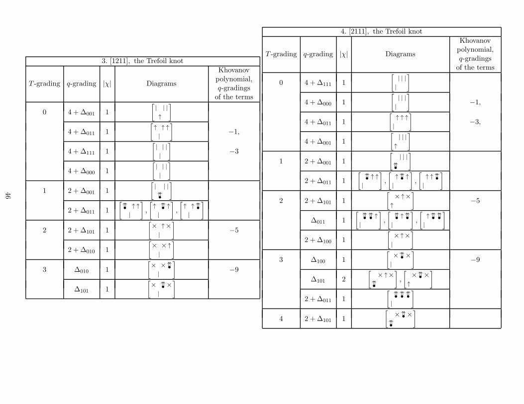
3. [1211], the Trefoil knot
T -grading q-grading |χ| Diagrams
Khovanovpolynomial,q-gradingsof the terms
0 4 + ∆001 1
[| | |
↑
]
4 + ∆011 1
[↑ ↑ ↑
|
]
−1,
4 + ∆111 1
[| | |
|
]
−3
4 + ∆000 1
[| | |
|
]
1 2 + ∆001 1
[| | |
↑↑•
]
2 + ∆011 1
[↑↑• ↑ ↑
|
]
,
[↑ ↑↑• ↑
|
]
,
[↑ ↑ ↑↑•|
]
2 2 + ∆101 1
[× ↑×
|
]
−5
2 + ∆010 1
[× × ↑
|
]
3 ∆010 1
[× × ↑↑•
|
]
−9
∆101 1
[× ↑↑• ×
|
]
4. [2111], the Trefoil knot
T -grading q-grading |χ| Diagrams
Khovanovpolynomial,q-gradingsof the terms
0 4 +∆111 1
[| | |
|
]
4 +∆000 1
[| | |
|
]
−1,
4 +∆011 1
[↑ ↑ ↑
|
]
−3,
4 +∆001 1
[| | |
↑
]
1 2 +∆001 1
[| | |
↑↑•
]
2 +∆011 1
[↑↑• ↑ ↑
|
]
,
[↑ ↑↑• ↑
|
]
,
[↑ ↑ ↑↑•
|
]
2 2 +∆101 1
[× ↑×
↑
]
−5
∆011 1
[↑↑• ↑↑• ↑
|
]
,
[↑↑• ↑ ↑↑•
|
]
,
[↑ ↑↑• ↑↑•
|
]
2 +∆100 1
[× ↑×|
]
3 ∆100 1
[× ↑↑• ×|
]
−9
∆101 2
[× ↑×
↑↑•
]
,
[× ↑↑• ×
↑
]
2 +∆011 1
[↑↑• ↑↑• ↑↑•
|
]
4 2 +∆101 1
[× ↑↑• ×
↑↑•
]
46

5. [1222], the Trefoil knot
T -grading q-grading |χ| Diagrams
Khovanovpolynomial,q-gradingsof the terms
0 4 + ∆001 1
[|
↑ ↑ ↑
]
4 + ∆011 1
[↑
| | |
]
−1,
4 + ∆111 1
[|
| | |
]
−3
4 + ∆000 1
[|
| | |
]
1 2 + ∆001 1
[|
↑↑• ↑ ↑
]
,
[|
↑ ↑↑• ↑
]
,
[|
↑ ↑ ↑↑•
]
2 + ∆011 1
[↑↑•
| | |
]
2 2 + ∆110 1
[|
× ↑×
]
∆001 1
[|
↑↑• ↑↑• ↑
]
,
[|
↑↑• ↑ ↑↑•
]
,
[|
↑ ↑↑• ↑↑•
]
−5
2 + ∆010 1
[↑
× ↑×
]
3 ∆110 1
[|
× ↑↑• ×
]
∆010 2
[↑↑•
× ↑×
]
,
[↑
× ↑↑• ×
]
−9
2 + ∆001 1
[|
↑↑• ↑↑• ↑↑•
]
4 2 + ∆010 1
[↑↑•
× ↑↑• ×
]
6. [2122], the Trefoil knot
T -grading q-grading |χ| Diagrams
Khovanovpolynomial,q-gradingsof the terms
0 4 + ∆111 1
[|
| | |
]
4 + ∆000 1
[|
| | |
]
−1,
4 + ∆011 1
[↑
| | |
]
−3
4 + ∆001 1
[|
↑ ↑ ↑
]
1 2 + ∆001 1
[|
↑↑• ↑ ↑
]
,
[|
↑ ↑↑• ↑
]
,
[|
↑ ↑ ↑↑•
]
2 + ∆011 1
[↑↑•
| | |
]
2 2 + ∆101 1
[|
× × ↑
]
−5
2 + ∆010 1
[|
× ↑×
]
3 ∆101 1
[|
× × ↑↑•
]
−9
∆010 1
[|
× ↑↑• ×
]
47
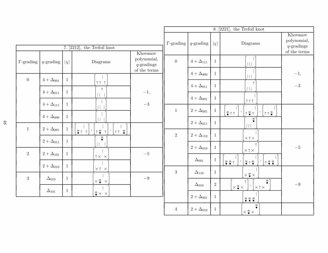
7. [2212], the Trefoil knot
T -grading q-grading |χ| Diagrams
Khovanovpolynomial,q-gradingsof the terms
0 4 + ∆001 1
[|
↑ ↑ ↑
]
4 + ∆011 1
[↑
| | |
]
−1,
4 + ∆111 1
[|
| | |
]
−3
4 + ∆000 1
[|
| | |
]
1 2 + ∆001 1
[|
↑↑• ↑ ↑
]
,
[|
↑ ↑↑• ↑
]
,
[|
↑ ↑ ↑↑•
]
2 + ∆011 1
[↑↑•
| | |
]
2 2 + ∆101 1
[|
↑× ×
]
−5
2 + ∆010 1
[|
× ↑ ×
]
3 ∆010 1
[|
× ↑↑• ×
]
−9
∆101 1
[|
↑↑• × ×
]
8. [2221], the Trefoil knot
T -grading q-grading |χ| Diagrams
Khovanovpolynomial,q-gradingsof the terms
0 4 +∆111 1
[|
| | |
]
4 +∆000 1
[|
| | |
]
−1,
4 +∆011 1
[↑
| | |
]
−3
4 +∆001 1
[|
↑ ↑ ↑
]
1 2 +∆001 1
[|
↑↑• ↑ ↑
]
,
[|
↑ ↑↑• ↑
]
,
[|
↑ ↑ ↑↑•
]
2 +∆011 1
[↑↑•
| | |
]
2 2 +∆110 1
[|
× ↑×
]
2 +∆010 1
[↑
× ↑×
]
−5
∆001 1
[|
↑↑• ↑↑• ↑
]
,
[|
↑↑• ↑ ↑↑•
]
,
[|
↑ ↑↑• ↑↑•
]
3 ∆110 1
[|
× ↑↑• ×
]
∆010 2
[↑
× ↑↑• ×
]
,
[↑↑•
× ↑×
]
−9
2 +∆001 1
[|
↑↑• ↑↑• ↑↑•
]
4 2 +∆010 1
[↑↑•
× ↑↑• ×
]
48

9. [1212]., the Trefoil knot
T -grading q-grading |χ| Diagrams
Khovanovpolynomial,q-gradingsof the terms
0 4 + ∆111 1
[| |
| |
]
4 + ∆000 1
[| |
| |
]
−1,
4 + ∆011 1
[↑ ↑
| |
]
−3
4 + ∆001 1
[| |
↑ ↑
]
1 2 + ∆001 1
[| |
↑↑• ↑
]
,
[| |
↑ ↑↑•
]
2 + ∆011 1
[↑↑• ↑
| |
]
,
[↑ ↑↑•| |
]
2 2 + ∆101 1
[× ×
| ↑
]
−5
2 + ∆010 1
[↑ |
× ×
]
3 ∆101 1
[× ×
| ↑↑•
]
−9
∆010 1
[↑↑• |
× ×
]
10. [2121], the Trefoil knot
T -grading q-grading |χ| Diagrams
Khovanovpolynomial,q-gradingsof the terms
0 4 + ∆001 1
[| |
↑ ↑
]
4 + ∆011 1
[↑ ↑
| |
]
−1,
4 + ∆111 1
[| |
| |
]
−3
4 + ∆000 1
[| |
| |
]
1 2 + ∆001 1
[| |
↑↑• ↑
]
,
[| |
↑ ↑↑•
]
2 + ∆011 1
[↑↑• ↑
| |
]
,
[↑ ↑↑•
| |
]
2 2 + ∆101 1
[× ×
↑ |
]
−5
2 + ∆010 1
[| ↑
× ×
]
3 ∆010 1
[| ↑↑•
× ×
]
−9
∆101 1
[× ×
↑↑• |
]
49

E.3 The “thick” knot 819 (torus T [3, 4])
[12122122], knot 819, or torus T [3, 4]
T -gr. q-gr. |χ| DiagramsKh.pol.,q-grds.
0 8 + ∆000 1
[
| | || | | | |
]
.
8 + ∆111 1
[
| | || | | | |
]
. 5,
8 + ∆011 1
[
↑ ↑ ↑| | | | |
]
. 7
8 + ∆001 1
[
| | |↑ ↑ ↑ ↑ ↑
]
.
1 6 + ∆011 1
[
↑↑• ↑ ↑
| | | | |
]
,
[
↑ ↑↑• ↑
| | | | |
]
,
[
↑ ↑ ↑↑•| | | | |
]
.
6 + ∆001 1
[
| | |↑↑• ↑ ↑ ↑ ↑
]
,
[
| | |
↑ ↑↑• ↑ ↑ ↑
]
,
[
| | |
↑ ↑ ↑↑• ↑ ↑
]
,
[
| | |
↑ ↑ ↑ ↑↑• ↑
]
,
[
| | |
↑ ↑ ↑ ↑ ↑↑•
]
.
2 6 + ∆010 1
[
↑ | |× ↑ ↑ ↑×
]
. 9
6 + ∆101 1
[
× ↑ ×| | | ↑ ↑
]
.
3 4 + ∆010 1
[
↑↑• | |
× ↑ ↑ ↑×
]
,
[
↑ | |
× ↑↑• ↑ ↑×
]
,
[
↑ | |
× ↑ ↑↑• ↑×
]
,
[
↑ | |
× ↑ ↑ ↑↑• ×
]
. 13
4 + ∆101 1
[
× ↑↑• ×
| | | ↑ ↑
]
,
[
× ↑ ×
| | | ↑↑• ↑
]
,
[
× ↑ ×
| | | ↑ ↑↑•
]
.
4 4 + ∆100 1
[
× | ×× ↑× | |
]
. 11,
2 + ∆001 1
[
| | ↑↑↑• ↑↑• × × ↑
]
,
[
| | |↑↑• ↑↑• ↑ ××
]
,
[
| | |↑↑• ×× ↑↑• ↑
]
,
[
| | |↑↑• ×× ↑ ↑↑•
]
,
[
| | |↑↑• ↑ ↑↑• ××
]
,
[
| | ↑↑•↑↑• ↑× × ↑
]
,
[
| | ↑↑↑• ↑ × × ↑↑•
]
,
[
| ↑↑• |
× × ↑↑• ↑ ↑
]
,
[
| ↑↑• |
× × ↑ ↑↑• ↑
]
,
[
| ↑↑• |
× × ↑ ↑ ↑↑•
]
,
[
| ↑ |
× × ↑↑• ↑↑• ↑
]
,
[
| ↑ |
× × ↑↑• ↑ ↑↑•
]
,
[
| ↑ |
× ×↑ ↑↑• ↑↑•
]
,
[
| | |
↑ ↑↑• ↑↑• ××
]
,
[
| | ↑↑•↑ ↑↑• × × ↑
]
,
[
| | ↑
↑ ↑↑• × × ↑↑•
]
,
[
| | |
↑ ×× ↑↑• ↑↑•
]
,
[
| | ↑↑•↑ ↑ × × ↑↑•
]
.
13
4 + ∆110 1
[
| × ×× | | ↑×
]
.
2 + ∆011 1
[
↑↑• × ×
| ↑↑• ↑ | |
]
,
[
↑↑• × ×
| ↑ ↑↑• | |
]
,
[
× × ↑↑•↑↑• | | | |
]
,
[
↑ × ×
| ↑↑• ↑↑• | |
]
.
5 ∆001 1
[
| | |↑↑• ↑↑• ↑↑• ××
]
,
[
| | ↑↑•↑↑• ↑↑• × × ↑
]
,
[
| | ↑↑↑• ↑↑• × × ↑↑•
]
,
[
| | |↑↑• ×× ↑↑• ↑↑•
]
,
[
| | ↑↑•↑↑• ↑× × ↑↑•
]
,
[
| ↑↑• |
× × ↑↑• ↑↑• ↑
]
,
[
| ↑↑• |
× × ↑↑• ↑ ↑↑•
]
,
[
| ↑↑• |
× × ↑ ↑↑• ↑↑•
]
,
[
| ↑ |
× ×↑↑• ↑↑• ↑↑•
]
,
[
| | ↑↑•↑ ↑↑• × × ↑↑•
]
.
2 + ∆100 1
[
× | ×
× ↑↑• × | |
]
. 15,
2 + ∆110 1
[
| × ×
× | | ↑↑• ×
]
. 17
∆011 1
[
↑↑• × ×
| ↑↑• ↑↑• | |
]
.
50