Khinchine type inequalities with optimal constants via ultra log-concavity

Positivity (2012) 16:359–371DOI 10.1007/s11117-011-0130-z Positivity

Khinchine type inequalities with optimal constantsvia ultra log-concavity

Piotr Nayar · Krzysztof Oleszkiewicz

Received: 30 March 2011 / Accepted: 23 May 2011 / Published online: 15 June 2011© The Author(s) 2011. This article is published with open access at Springerlink.com

Abstract We derive Khinchine type inequalities for even moments with optimalconstants from the result of Walkup (J Appl Probab 13:76–85, 1976) which states thatthe class of log-concave sequences is closed under the binomial convolution.

Keywords Log-concavity · Ultra log-concavity · Khinchine inequality ·Factorial moments

Mathematics Subject Classification (2000) 60E15 · 26D15

1 Introduction

Let α1, α2, . . . , αn ∈ R and let r1, r2, . . . , rn be independent symmetric ±1 randomvariables. The classical Khinchine inequality [8], states that for any positive p > qthere exists a constant C p,q (which does not depend on n, α1, α2, . . . , αn) such that

(E|S|p)1/p ≤ C p,q · (E|S|q)1/q ,

where S = ∑ni=1 αi ri .

Research of K. Oleszkiewicz was partially supported by Polish MNiSzW Grant N N201 397437.

P. Nayar (B) · K. OleszkiewiczInstitute of Mathematics, University of Warsaw,ul. Banacha 2, 02-097 Warsaw, Polande-mail: [email protected]

K. OleszkiewiczInstitute of Mathematics, Polish Academy of Sciences,ul. Sniadeckich 8, 00-956 Warsaw, Polande-mail: [email protected]

360 P. Nayar, K. Oleszkiewicz

There was a long pursuit for the optimal values of the constants C p,q . The bestvalues of C p,2 for p ≥ 3 were established by Whittle [16] while the optimal C2,1

constant was proved to be equal to√

2 by Szarek [14] (see also [12] for a short proofwhich extends to the normed linear space setting; this approach was later extended in[10,13]). Finally, Haagerup [6], found best values of C p,2 for all p ∈ (2, 3), and ofC2,q for all q ∈ (0, 2), thus solving the part of the problem which is most importantfor applications since E S2 = ∑n

i=1 α2i is a quantity particularly easy to deal with.

However, the general problem of finding optimal values of the constants C p,q is openand probably quite difficult. Its special case when both p and q are even numbers,and p is divisible by q, was settled by Czerwinski in his unpublished Master thesis[4]. His method was based on some algebraic-combinatorial identities and does notseem to generalize to other situations. On the other hand, König and Kwapien [9],and Baernstein and Culverhouse [1], have obtained comparison of moments inequal-ities with best constants, similar in spirit to Haagerup’s result but with the symmetricBernoulli random variables replaced by some multidimensional rotationally invari-ant random vectors of special form (for example, uniformly distributed on spheres orballs). Again, as in Haagerup’s approach, it was crucial for their main argument towork to have p = 2 or q = 2. In the present paper we establish the optimal valuesof C p,q for even p > q > 0 (the assumption of q | p no longer needed) both in theclassical Khinchine inequality and its high-dimensional counterparts.

The main tool in our approach is Walkup’s theorem (Theorem 1 of [15]) which statesthat the binomial convolution of two log-concave sequences is also log-concave:

Definition 1 A sequence (ai )∞i=0 of non-negative real numbers is called log-concave

if a2i ≥ ai−1ai+1 for i ≥ 1 and the set {i ≥ 0 | ai > 0} is an interval of integers.

Theorem 1 (Walkup [15]) Let (ai )∞i=0 and (bi )

∞i=0 be two log-concave sequences of

positive real numbers. Define

cn =n∑

i=0

(n

i

)

ai bn−i .

Then the sequence (cn)∞n=0 is log-concave.

Using Liggett’s terminology [11] we may also rephrase this to another statement:the class of ultra log-concave sequences is closed under standard convolution opera-tion, where a sequence of positive numbers (ai )

∞i=0 is called ultra log-concave if and

only if the sequence (i ! · ai )∞i=0 is log-concave.

There are at least three proofs of this theorem in the literature. Walkup’s originalproof is a bit difficult for non-experts whereas Liggett’s proof [11] is very elementarybut quite long, as it covers a more general result than just Theorem 1. Recently, Gurvits[5] published a short proof which, however, relies on the powerful Alexander-Fenchelinequalities for mixed volumes of convex bodies. For reader’s convenience we pro-vide yet another proof, more similar to Liggett’s than to Walkup’s, but shorter thanLiggett’s proof and very direct. We postpone it till Sect. 3.

Khinchine type inequalities with optimal constants 361

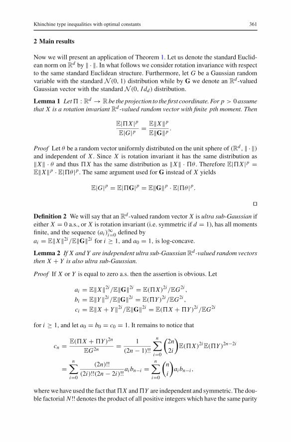
2 Main results

Now we will present an application of Theorem 1. Let us denote the standard Euclid-ean norm on R

d by ‖ · ‖. In what follows we consider rotation invariance with respectto the same standard Euclidean structure. Furthermore, let G be a Gaussian randomvariable with the standard N (0, 1) distribution while by G we denote an R

d -valuedGaussian vector with the standard N (0, I dd) distribution.

Lemma 1 Let � : Rd → R be the projection to the first coordinate. For p > 0 assume

that X is a rotation invariant Rd -valued random vector with finite pth moment. Then

E|�X |p

E|G|p= E‖X‖p

E‖G‖p.

Proof Let θ be a random vector uniformly distributed on the unit sphere of (Rd , ‖ · ‖)and independent of X . Since X is rotation invariant it has the same distribution as‖X‖ · θ and thus �X has the same distribution as ‖X‖ · �θ . Therefore E|�X |p =E‖X‖p · E|�θ |p. The same argument used for G instead of X yields

E|G|p = E|�G|p = E‖G‖p · E|�θ |p.

Definition 2 We will say that an R

d -valued random vector X is ultra sub-Gaussian ifeither X = 0 a.s., or X is rotation invariant (i.e. symmetric if d = 1), has all momentsfinite, and the sequence (ai )

∞i=0 defined by

ai = E‖X‖2i/E‖G‖2i for i ≥ 1, and a0 = 1, is log-concave.

Lemma 2 If X and Y are independent ultra sub-Gaussian Rd-valued random vectors

then X + Y is also ultra sub-Gaussian.

Proof If X or Y is equal to zero a.s. then the assertion is obvious. Let

ai = E‖X‖2i/E‖G‖2i = E(�X)2i/EG2i ,

bi = E‖Y‖2i/E‖G‖2i = E(�Y )2i/EG2i ,

ci = E‖X + Y‖2i/E‖G‖2i = E(�X + �Y )2i/EG2i

for i ≥ 1, and let a0 = b0 = c0 = 1. It remains to notice that

cn = E(�X + �Y )2n

EG2n= 1

(2n − 1)!!n∑

i=0

(2n

2i

)

E(�X)2iE(�Y )2n−2i

=n∑

i=0

(2n)!!(2i)!!(2n − 2i)!!ai bn−i =

n∑

i=0

(n

i

)

ai bn−i ,

where we have used the fact that �X and �Y are independent and symmetric. The dou-ble factorial N !! denotes the product of all positive integers which have the same parity


as N and do not exceed N . We adopt the standard convention that (−1)!! = 0!! = 1.

The assertion immediately follows from Theorem 1. Lemma 3 Assume that an R

d-valued random vector X and a non-negative randomvariable R are independent, and that R · X has distribution N (0, I dd). Then X isultra sub-Gaussian.

Proof Clearly, X is rotation invariant. Note that for p > 0 we have

E‖X‖p · ER p = E‖G‖p ∈ (0,∞),

so that X has all moments finite and strictly positive. Let ai = E‖X‖2i/E‖G‖2i . Bythe Schwarz inequality for i ≥ 1 we have

1/a2i = (ER2i )2 ≤ ER2(i−1) · ER2(i+1) = 1/(ai−1ai+1)

which proves that the sequence (ai )∞i=0 is log-concave.

Corollary 1 Assume that X is a random vector uniformly distributed on

(i) the Euclidean sphere r · Sd−1 (if d = 1 this is symmetric ±r distribution)or

(ii) the Euclidean ball r · Bd

for some r > 0. Then X is ultra sub-Gaussian.

Proof Distribution of any Rd -valued random vector which is rotation invariant and

unimodal (i.e. it has a rotation invariant density which is non-increasing as a functionof distance to zero) can be expressed as an integral mean of measures uniformly dis-tributed on balls with center in zero. Since the standard normal distribution N (0, I dd)

is rotation invariant and unimodal the corollary is established in the case (ii).For the reader’s convenience, however, we provide an explicit description of this

factorization. Let us denote the volume of the unit ball Bd by vd = πd/2/�( d2 + 1)

and let ϕd(s) = (2π)−d/2e−s2/2, i.e. ϕd(‖x‖) is a density of N (0, I dd). Furthermore,for s > 0 set us(x) = v−1

d s−d1{x∈Rd :‖x‖≤s}, so that us is a density of a random vectoruniformly distributed on s · Bd . Hence

ϕd(‖x‖) =∞∫

‖x‖(−ϕ′

d(s)) ds =∞∫

0

1{x∈Rd :‖x‖≤s}sϕd(s) ds

=∞∫

0

vdsd+1ϕd(s)us(x) ds.

Thus the product of a random vector uniformly distributed on Bd with an indepen-dent positive random variable R with density vdsd+1ϕd(s)1(0,∞)(s) has distributionN (0, I dd). Setting R = R/r ends the construction.


The case (i) is simpler, it just suffices to note that

G = ‖G‖r

· rG

‖G‖ ,

where the factors are independent, and the second of them is uniformly distributed onr · Sd−1. Corollary 2 For α > 0 let X be an R

d -valued random vector with density

gX (x) = �( d2 + 1)

�( dα

+ 1)π−d/2e−‖x‖α

.

If α > 2 then X is ultra sub-Gaussian.

Proof Let β ∈ (0, α) and let Y be an Rd -valued random vector with density

gY (x) = �( d2 + 1)

�( dβ

+ 1)π−d/2e−‖x‖β

.

It is a well-known fact that Y is a mixture of dilatations of X and thus (for β = 2 < α)the assertion follows. For the sake of completeness we provide a detailed argument.Let Z be a standard positive β/α-stable random variable, so that Ee−wZ = e−wβ/α

forevery w ≥ 0. Note that for μ > 0 we have

EZ−μ = E1

�(μ)

∞∫

0

e−t Z tμ−1 dt = 1

�(μ)

∞∫

0

tμ−1Ee−t Z dt

= 1

�(μ)

∞∫

0

tμ−1e−tβ/α

dt = α�(αμ/β)

β�(μ).

Let gZ denote the density of Z and let W be a positive random variable independentof X with density

gW (t) = β�(d/α)

α�(d/β)t−d/αgZ (t).

We will prove that W −1/α X has the same distribution as Y . Since both random vectorsare rotation invariant it suffices to prove that W −1/α‖X‖ has the same distribution as‖Y‖ which immediately follows from the fact that the Laplace transforms of logarithmsof these random variables are equal:

E(W −1/α‖X‖)λ = EW −λ/α · E‖X‖λ = E‖Y‖λ


for every λ ≥ 0. Indeed, by a standard and direct computation we obtain E‖X‖λ =�(λ+d

α)/�(d/α) and E‖Y‖λ = �(λ+d

β)/�(d/β), whereas

EW −λ/α = β�(d/α)

α�(d/β)EZ−(λ+d)/α = �(d/α)�(λ+d

β)

�(d/β)�(λ+dα

).

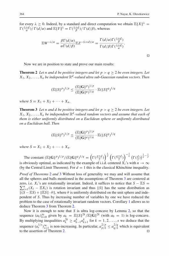
Now we are in position to state and prove our main results:

Theorem 2 Let n and d be positive integers and let p > q ≥ 2 be even integers. LetX1, X2, . . . , Xn be independent R

d-valued ultra sub-Gaussian random vectors. Then

(E‖S‖p)1/p ≤ (E‖G‖p)1/p

(E‖G‖q)1/q· E(‖S‖q)1/q

where S = X1 + X2 + · · · + Xn.

Theorem 3 Let n and d be positive integers and let p > q ≥ 2 be even integers. LetX1, X2, . . . , Xn be independent R

d -valued random vectors and assume that each ofthem is either uniformly distributed on a Euclidean sphere or uniformly distributedon a Euclidean ball. Then

(E‖S‖p)1/p ≤ (E‖G‖p)1/p

(E‖G‖q)1/q· E(‖S‖q)1/q

where S = X1 + X2 + · · · + Xn.

The constant (E‖G‖p)1/p/(E‖G‖q)1/q =(�(

p+d2 )

) 1p(�(

q+d2 )

)− 1q (

�( d2 )

) 1q − 1

p

is obviously optimal, as indicated by the example of i.i.d. centered Xi ’s with n → ∞(by the Central Limit Theorem). For d = 1 this is the classical Khinchine inequality.

Proof of Theorems 2 and 3 Without loss of generality we may and will assume thatall the spheres and balls mentioned in the assumptions of Theorem 3 are centered atzero, i.e. Xi ’s are rotationally invariant. Indeed, it suffices to notice that S − ES =∑n

i=1(Xi − EXi ) is rotation invariant and thus ‖S‖ has the same distribution as‖(S − ES) + ‖ES‖ · θ‖, where θ is uniformly distributed on the unit sphere and inde-pendent of S. Thus by increasing number of variables by one we have reduced theproblem to the case of rotationally invariant random vectors. Corollary 1 allows us todeduce Theorem 3 from Theorem 2.

Now it is enough to note that S is ultra log-concave by Lemma 2, so that thesequence (ak)

∞k=0 given by ak = E‖S‖2k/E‖G‖2k (with a0 = 1) is log-concave.

By multiplying inequalities a2kk ≥ ak

k−1akk+1 for k = 1, 2, . . . , s we deduce that the

sequence (a1/ss )∞s=1 is non-increasing. In particular, a2/p

p/2 ≤ a2/qq/2 which is equivalent

to the assertion of Theorem 2.


3 Proof of Walkup’s theorem

We assume that(n

k

) = 0 for k < 0 and k > n, where n ≥ 0, k, n ∈ Z. Let us also setai = bi = 0 for i < 0, i ∈ Z.

Lemma 4 Let n ≥ 1 and k ≤ n be non-negative integers. Then

(n + 1

i

)(n − 1

k − i

)

≥(

n + 1

k − i + 1

)(n − 1

i − 1

)

(1)

for 0 ≤ i ≤ �k/2 .

Proof For i = 0 the inequality (1) is obvious. For i > 0 it is equivalent to

(n − k + i)(k − i + 1) ≥ i(n + 1 − i).

Since n ≥ k and i ≤ k/2 we have

(n − k + i)(k − i + 1) − i(n + 1 − i) = (n − k)(k − 2i + 1) ≥ 0.

Lemma 5 For n ≥ 1, k ≤ n and 0 ≤ i ≤ �k/2 consider a sequence

si = 2

(n

i

)(n

k − i

)

−(

n − 1

i

)(n + 1

k − i

)

−(

n + 1

i

)(n − 1

k − i

)

.

Then the sequence (sgn(si ))�k/2 i=0 is non-decreasing.

Proof After some simple reductions we get

sgn(si ) = sgn

[2n

n + 1− n − i

n − k + i + 1− n − k + i

n + 1 − i

]

.

Let m = n − k ≥ 0. We have

n−i

n−k+i +1+ n−k+i

n+1−i= m+n+1

m+i +1−1+ m+n+1

n+1−i−1 = (m+n+1)(m+n+2)

(m+i +1)(n+1−i)−2

therefore it suffices to notice that the function i �→ (m + i + 1)(n + 1 − i) is positiveand non-decreasing on [0, k/2]. Lemma 6 Let (si )

ni=0, (li )

ni=0 be two sequences of real numbers. Assume that 0 ≤

l1 ≤ l2 · · · ≤ ln,∑n

i=0 si = 0 and the sequence (sgn(si ))ni=0 is non-decreasing. Then∑n

i=0 si li ≥ 0.


Proof Let i0 = min{0 ≤ i ≤ n | si ≥ 0}. Then

n∑

i=0

si li =∑

i<i0

si li +∑

i≥i0

si li ≥ li0

∑

i<i0

si + li0

∑

i≥i0

si = 0.

Before we give a proof of Theorem 1, let us make some remarks. Let (ai )

∞i=0, (bi )

∞i=0

be log-concave. Fix 1 ≤ i ≤ j . Observe that

ai a j ≥ ai−1a j+1, for 0 ≤ i ≤ j. (2)

Indeed, it suffices to consider the case when ai−1 and a j+1 are positive. Then {i −1, i, . . . , j, j +1} ⊂ {k ≥ 0 | ak > 0}. By multiplying the inequalities a2

k ≥ ak−1ak+1

for k = i, . . . , j and dividing by ai a2i+1 · . . . a2

j−1a j > 0 we arrive at (2). Note thatwe have used the fact that {k ≥ 0 | ak > 0} is an interval of integers.

If 0 ≤ i ≤ j and 0 ≤ k ≤ l then from (2) we get

(ai a j − ai−1a j+1)(bkbl − bk−1bl+1) ≥ 0,

therefore

ai a j bkbl +ai−1a j+1bk−1bl+1 ≥ai a j bk−1bl+1 + ai−1a j+1bkbl , 0≤ i ≤ j, 0≤k ≤ l.

(3)

For fixed k, n, k ≤ n we will use the notation Li = ai ak−i bn−i bn−k+i and Ri =ai ak−i bn−i+1bn−k+i−1. Note that Li = Lk−i and L−1 = 0.

Proof of Theorem 1 It is easy to check that the set {i ≥ 0 | ci > 0} is an interval ofintegers. Therefore, for n ≥ 1 we have to prove the inequality

∑

j=0,...,ni=0,...,n

(n

i

)(n

j

)

ai a j bn−i bn− j ≥∑

j=0,...,n−1i=0,...,n+1

(n+1

i

)(n−1

j

)

ai a j bn+1−i bn−1− j .

It suffices to prove that

k∑

i=0

(n

i

)(n

k − i

)

ai ak−i bn−i bn−k+i ≥k∑

i=0

(n + 1

i

)(n − 1

k − i

)

ai ak−i bn+1−i bn−1−k+i

(4)

for k = 0, . . . , 2n. Inequality (4) for k ≥ n and a pair ((ai )∞i=0, (bi )

∞i=0) is equivalent

to (4) for k = 2n −k ≤ n and a pair ((bi )∞i=0, (ai )

∞i=0), so we can consider only k ≤ n.


For i = 0, . . . , �k/2 we have i ≤ k − i and n − k + i ≤ n − i, therefore (3) yields

(n + 1

k − i + 1

)(n − 1

i − 1

)

(ai ak−i bn−i bn−k+i + ai−1ak−i+1bn−i+1bn−k+i−1)

≥(

n + 1

k − i + 1

)(n − 1

i − 1

)

(ai ak−i bn−i+1bn−k+i−1 + ai−1ak−i+1bn−i bn−k+i ).

Moreover, using Lemma 4 and (2) we have

[(n + 1

i

)(n − 1

k − i

)

−(

n + 1

k − i + 1

)(n − 1

i − 1

)]

ai ak−i bn−i+1bn−k+i−1

≤[(

n + 1

i

)(n − 1

k − i

)

−(

n + 1

k − i + 1

)(n − 1

i − 1

)]

ai ak−i bn−i bn−k+i .

We can rewrite these inequalities in the form of

(n + 1

k − i + 1

)(n − 1

i − 1

)

(Li + Li−1) ≥(

n + 1

k − i + 1

)(n − 1

i − 1

)

(Ri + Rk−i+1) (5)

and

[(n + 1

i

)(n − 1

k − i

)

−(

n + 1

k − i + 1

)(n − 1

i − 1

)]

Li ≥[(

n + 1

i

)(n − 1

k − i

)

−(

n + 1

k − i + 1

)(n − 1

i − 1

)]

Ri (6)

for i = 0, . . . , �k/2 . Note that if k is odd then L�k/2 = R�k/2 +1. In order to estimatethe RHS of (4) we add (5) and (6) for i = 0, . . . , �k/2 , and the equality

(n − 1

�k/2 )(

n + 1

k − �k/2 )

L�k/2 =(

n − 1

�k/2 )(

n + 1

k − �k/2 )

R�k/2 +1

in the case of k odd. We arrive at

k∑

i=0

(n+1

i

)(n−1

k−i

)

Ri ≤�k/2 −1∑

i=0

[(n − 1

i

)(n + 1

k − i

)

+(

n + 1

i

)(n − 1

k − i

)]

Li

+θk

[(n−1

�k/2 )(

n+1

k−�k/2 )

+(

n+1

�k/2 )(

n−1

k−�k/2 )]

L�k/2 ,

where θk = 1/2 if k is even and θk = 1 when k is odd. Since the LHS of (4) is equal to

�k/2 −1∑

i=0

2

(n

i

)(n

k − i

)

Li + 2θk

(n

�k/2 )(

n

k − �k/2 )

L�k/2 ,


it suffices to prove the inequality

�k/2 −1∑

i=0

si Li + θks�k/2 L�k/2 ≥ 0.

We have

�k/2 −1∑

i=0

si + θks�k/2 = 1

2

k∑

i=0

si = 0

and 0 ≤ L0 ≤ L1 ≤ · · · ≤ L�k/2 . To finish the proof it suffices to use Lemma 5 andLemma 6. Remark 1 Consider sequences (an)∞n=0 = (1, 0, 0, 1, 0, 0, . . .) and (bn)∞n=0 =(1, 1,

1, . . .) and note that the binomial convolution of these sequences is not log-concave.Therefore, without the second assumption in the Definition (1) it is impossible to proveWalkup’s Theorem.

4 Inequalities for factorial moments

For a positive integer n and any real number x we define the Pochhammer symbol(x)n = x(x − 1) · . . . · (x − n + 1), with (x)0 = 1, and in a standard way we put(x

n

) = (x)n/n!. Let n be a non-negative integer and let X be a nonnegative randomvariable X with E|X |n < ∞. Then E(X)n is called the nth factorial moment of X .

Definition 3 Let κ ∈ R. We will say that a nonnegative integer-valued random vari-able X is κ-good if the sequence Eeκ X (X)n for n ≥ 0 is log-concave (we assume thatall the expectations are finite).

Lemma 7 If X and Y are independent κ-good random variables then X + Y is alsoκ-good.

Proof Multiplying the obvious identity

eκ(X+Y )

(X + Y

k

)

=k∑

i=0

eκ X(

X

i

)

· eκY(

Y

k − i

)

by k! we arrive at

eκ(X+Y )(X + Y )k =k∑

i=0

(k

i

)

eκ X (X)i · eκY (Y )k−i .

To finish the proof it suffices to take expectation of both sides of this equality, useTheorem 1 and independence of X and Y .


Now we can conclude with the following inequality:

Theorem 4 Let κ ∈ R and let X1, X2, . . . , Xn be independent κ-good random vari-ables (e.g. {0, 1} Bernoulli random variables) and let p be a positive integer. Then forS = X1 + X2 + · · · + Xn we have

(EeκS(S)p)2 ≥ EeκS(S)p−1 · EeκS(S)p+1.

Since limκ→−∞ e−κpEeκ X (X)p = p! · P(X = p) the case of κ → −∞ refers to

the ultra log-concavity of the sequence P(X = p) which was carefully investigatedand successfully applied for example in a recent paper of Johnson [7]. In fact, thelog-concavity of the sequence EeκS(S)p may be easily deduced from the ultra log-concavity of the sequence P(S = p), which in particular covers the case of Bernoullisums. However, sometimes the sequence E(X)p or, more generally, E(X)peκ X maybe log-concave even though the sequence P(X = p) is not ultra log-concave.

5 Tail to moments log-concavity trick

We finish with a discussion of a result of Borell ([3], formulated there in a slightlydifferent and more general setting) which, in fact, can be traced back to the work ofBarlow, Marshall, and Proschan [2, p. 384] although there it appears with a slighltyrestricting additional assumption. It is very standard by now and has many differentproofs, some of them very simple, but still we think that it may be of some interest toprovide yet another argument, especially because it is quite similar in spirit to the onewe used in our proof of Walkup’s theorem.

Theorem 5 [2,3] Assume that ϕ : (0,∞) → (0,∞) is a log-concave function(i.e. log ϕ is concave). Then also � : (0,∞) → (0,∞) defined by

�(q) = 1

�(q)

∞∫

0

tq−1ϕ(t) dt

is log-concave.

Proof It suffices to prove that �(q)2 ≥ �(q − ε)�(q + ε) for q > ε > 0, whichobviously follows from

1

�(q)2

t∫

0

sq−1(t − s)q−1ϕ(s)ϕ(t − s) ds

≥ 1

�(q − ε)�(q + ε)

t∫

0

sq−ε−1(t − s)q+ε−1ϕ(s)ϕ(t − s) ds

by integration over t > 0 and using the Fubini theorem.


Since ϕ is log-concave the function s �→ ϕ(s)ϕ(t −s) is non-decreasing on (0, t/2]and non-increasing on [t/2, t). Also, it is obviously symmetric with respect to t/2.Hence it suffices to prove that

1

�(q)2

t−a∫

a

sq−1(t − s)q−1 ds ≥ 1

�(q − ε)�(q + ε)

t−a∫

a

sq−ε−1(t − s)q+ε−1 ds

for 0 < a < t/2, which upon using the homogeneity reduces to proving that

f (α)= B(q−ε, q+ε)

1−α∫

α

wq−1(1−w)q−1dw−B(q, q)

1−α∫

α

wq−ε−1(1−w)q+ε−1dw

is non-negative for α ∈ [0, 1/2]. Obviously, f (0) = f (1/2) = 0. Now it is enoughto notice that f ′(α) > 0 if and only if

(α

1 − α

)ε

+(

1 − α

α

)ε

> 2B(q − ε, q + ε)/B(q, q). (7)

The left hand side of (7) is decreasing in α, so that there exists some α0 ∈ (0, 1/2)

such that f is increasing on [0, α0] and then decreasing on [α0, 1/2]. Thus f ≥ 0 on[0, 1/2] and the proof is finished.

The following well known corollary follows (note that it reveals some intrigu-ing similarity to a way in which we used Walkup’s theorem to derive the Khinchineinequalities):

Corollary 3 Assume that Z is a positive random variable with log-concave tails, i.e.the function ϕ(t) = P(Z > t) is log-concave on (0,∞). Let E be an exponentialrandom variable with parameter 1. Then

(EZ p)1/p ≤ (EE p)1/p

(EEq)1/q· (EZq)1/q

for all p > q > 0.

The constant (EE p)1/p/(EEq)1/q = �(p + 1)1/p/�(q + 1)1/q obviously cannotbe improved in general since E has log-concave tails.

Proof From Theorem 5 we infer that � : [0,∞) → (0,∞) defined by

�(q) = 1

�(q)

∞∫

0

tq−1ϕ(t) dt = EZq

EEq

for q > 0, and by �(0) = 1, is log-concave (it is an easy exercise to check that �

is right-continuous at zero). Hence g(q) = log �(q) is concave with g(0) = 0, so


that q �→ g(q)/q is a non-increasing function on (0,∞), which is equivalent to theassertion of Corollary 3. Acknowledgments We are grateful to Matthieu Fradelizi and Olivier Guédon for pointing to us the articleof Walkup, and for their help in tracing some other references.

Open Access This article is distributed under the terms of the Creative Commons Attribution Noncom-mercial License which permits any noncommercial use, distribution, and reproduction in any medium,provided the original author(s) and source are credited.

References

1. Baernstein, II, A., Culverhouse, R.C.: Majorization of sequences, sharp vector Khinchin inequalities,and bisubharmonic functions. Stud. Math 152, 231–248 (2002)

2. Barlow, R.E., Marshall, A.W., Proschan, F.: Properties of probability distributions with monotonehazard rate. Ann. Math. Stat. 34, 375–389 (1963)

3. Borell, C.: Complements of Lyapunov’s inequality. Math. Ann. 205, 323–331 (1973)4. Czerwinski, W.: Khinchine inequalities (in Polish). University of Warsaw, Master thesis (2008)5. Gurvits, L.: A short proof, based on mixed volumes, of Liggett’s theorem on the convolution of ultra-

logconcave sequences. Electron. J. Combin. 16, Note 5 (2009)6. Haagerup, U.: The best constants in the Khintchine inequality. Stud. Math. 70, 231–283 (1982)7. Johnson, O.: Log-concavity and the maximum entropy property of the Poisson distribution. Stoch.

Process. Appl. 117, 791–802 (2007)8. Khintchine, A.: Über dyadische Brüche. Math. Z. 18, 109–116 (1923)9. König, H., Kwapien, S.: Best Khintchine type inequalities for sums of independent, rotationally invari-

ant random vectors. Positivity 5, 115–152 (2001)10. Kwapien, S., Latała, R., Oleszkiewicz, K.: Comparison of moments of sums of independent random

variables and differential inequalities. J. Funct. Anal. 136, 258–268 (1996)11. Liggett, T.M.: Ultra logconcave sequences and negative dependence. J. Combin. Theory Ser. A 79, 315–

325 (1997)12. Latała, R., Oleszkiewicz, K.: On the best constant in the Khinchin–Kahane inequality. Studia Math.

109, 101–104 (1994)13. Oleszkiewicz, K.: Comparison of moments via Poincaré-type inequality. In: Advances in Stochastic

Inequalities (Atlanta, GA, 1997), Contemp. Math. 234. American Mathematical Society, Providence135–148 (1999)

14. Szarek, S.: On the best constant in the Khintchine inequality. Stud. Math. 58, 197–208 (1976)15. Walkup, D.W.: Pólya sequences, binomial convolution and the union of random sets. J. Appl. Probab.

13, 76–85 (1976)16. Whittle, P.: Bounds for the moments of linear and quadratic forms in independent random variables.

Theory Probab. Appl. 5, 302–305 (1960)

Documents

Khinchine type inequalities with optimal constants via ultra log-concavity