q~4 RE-425J

kfi STRATEGY SYNTH-ESIS IN

P ARIAL DOGFIGHT GAME MODELS

BEST AVAILABLE COPY

April 1972

Reproduce by,

NATIOAL TEHNICA

INATORNATICHNSRICELSpringfield, Va. 22151

A~ 'R T.

* 4.4 4 "s

* -'- ' ,Xu 4~ ''Y

*1,7

Security Classi catlon ....14. LINK A LINK 8 LINK C

KEY W01405I

ROLE WT ROLE WT ROLE WT

Optimal Control TheoryGame TheoryMathematical ModelingFeedback Controls

Security Classification

n5, €dt¥ Cltam •Ifctlon ,, n , , - . .

DOCUMENT CONTROL DATA. R & D(1.IfHY c•I asse, Iication of .t ite, ba,. of ab.sract and indonxini nnrotiMlPm mull h. entered when the overall r•port a I ls.Iltid)

t, ORIGINATING ACTIVgiTO (Cofrporat. aithe1) 24. FtEPORT lKCUniTY CLASSIFICATION

Grumman Aerospace Corporation Unclassifiedab. GROUP

_______ _______ _______ _______N/A_ _ _ _ _ _

8. COfTONI TITLC

Strategy Synthesis in Aerial Dogfight Game Models

4. DESCRIPTIVE NOTES (T7ypo of report anid inrluive doles)

Research Report5. AU TNOR42) (Pirst name, mldd/. Initida. losl name)

Michael FalcoVictor Cohen

S. INIPORT DATE 7. TOTAL NO. OF PA4Ei 17b. NO. o Pr MKIS

April 1972 37 74. CONTRACT OR GRANT NO., Si. ORIGINATOR*S RiPORT NUM rERIS)

None RE-425Jb. PROJECT NO. R

0. M. OTHER REPORT mO45 (Any other numbers *at way be asIslmedA1. ,Spofl)

S None10. OISTRIUTION STATEMENT

Approved for public release; distribution unlimited

It., UPPLP9"N.,RY NOTES 1S. SPONSORING MILITARY ACTIVITY

None N/A

IS. ANi*ACTThe main problem of interest in this report is the "role-defini-tion problem" arising in one-on-one dogfight game models. The compu-tational approach is aimed at providing a decomposition of the spaceof game initial conditions into sets of unilateral capture capabilityfor each of the players, and at outlining the draw and sacrifice setsin accordance with the players' individual preferences for game out-comes. The procedure develops the feedback policy (in terms of the

observable data) that attains the above decomposition. Two highlysimplified one-on-one games are considered. The first game model is"a discrete time-state alternating move game (pvrfect information) on"a horizontal grid reminiscent of the Isaacs examples. The secondmodel is a continuous time-regional feedback game (imperfect infor-mation) in the horizontal plane. The strategy synthesis is effectedby a "reinforcement learning" procedure in both game models. Compu-tational results are given in some detail for the first game, whilepreliminary results are presented for the second game model.

DD ,OV 6,14 73 -- "

Security Clmsml(fc-tion

SI Grumman Research Department Report RE-425J

Ii

STRATEGY SYNTHESIS IN AERIAL DpOFIGHI CAME MODELSIbyI

M. Falco

and

V. Cohen

System Sciences

April 1972 DIDO

t Presented at the Air to Air Combat Analysis and Simulation Symposium,Kirtland Air Force Base, New Mexico, 29 February-2 March 1972. Tobe published in the Proceedings.

Approved by:Charles E. Mack, Jr.Director of Research

Approved for public reloese;I Distribution Unirnited

LJ[

STRATEGY SYNTHESIS IN AERIAL DOGFIGHT GAME MODELS

Michael Falco and Victor Cohen

Research DepartmentGrumman Aerospace Corporation

Bethpage, New York 11714

ABSTRACT

The main problem of interest in this paper is the "role-definition problem" arising in one-on-one dogfight gamemodels. The computational approach is aimed at providing adecomposition of the space of game initial conditions intosets of unilateral capture capability for each of the play-ers, and at outlining the draw and sacrifice sets in accor-dance with the players' individual preferences for game out-comes. The procedure develops the feedback policy (in termsof the observable data) that attains the above decomposition.Two highly simplified one-on-one games are considered. Thefirst game model is a discrete time-state alternating movegame (perfect information) on a horizontal grid reminiscentof the Isaacs examples. The second model is a continuoustime-regional feedback game (imperfect information) in thehorizontal plane. The strategy synthesis is cffected by a"reinforcement learning" procedure in both game models. Com-putational results are given in some detail for the firstgame, while preliminary results are presented for the secondgame model.

!!II ii

"[• I INTRODUCT ION

One of the more difficult areas for applications ori-ented workers in the field of modern optimal control theorycontinues to be the one-on-one aerial dogfight problem. Webelieve, in this case, these difficulties are due in part tothe fact that the one-on-one dogfight problem is perhapsmore accurately modeled as a "qualitative" differential game,as contrasted wit~i the "quantitative"game model. Briefly,the qualitative game is such that it contains two or moreevents dealing with termination of play, for which theplayers' have some preferential ordering, as contrasted withthe quantiative game for which real valued payoff functionsdefined on the trajectory and/or terminal data can be un-equivocally assumed as goals for each player, The Isaacs"homicidal chauffeur game" and "game of two cars" (Ref. 1)are pursuit games of the latter type. In these, the rolesof pursuer and evader are clear at the outset, and playersseek to minimize (and maximize) the capture time, respec-tively. Dogfight game models do not come equipped a prioriwith the pursuer and evader roles defined, in fact theserole definitions must be determined in the course of obtain-ing a resolution of these games.

The approach taken here is a small step in the directionof trying to resolve these dogfight game models. By resclu-tion, we mean to decompose the space of game initial condi-tions into sets of unilateral capture capability for eachplayer and to outline the sacrifice and draw sets in accor-dance with the players individual preferences for game out-comes, and furthermore to derive the associated strategies(providing the decomposition) as feedback control policieson the collection of observable data. Two highly simplifiedgame models are considered in the text. The first is a dis-crete time-state game with an alternating move structure.The second model is a continuous time-state game model em-ploying "regional" feedback policies. In the case of thefirst model, "perfect information" regarding the "state" ateach player's control decision has been assumed. A resolu-tion of that game model for specified dynamics, control capa-

.- bilities, weapons envelopes, and player preferences is ob-tained by two procedures. The first procedure is similar tothat employed by Isaacs (dynamic programming) in the homi-cidal chauffeur game, but with some modification to observethe stipulated preference descriptions of the dogfight in-stead of the min max capture time criteria of the chauffeur

II

V. game. The second procedure employs a "reinforcement rule"algorithm used in conjunction with the simulation of gameplays. The second procedure offers the conceptual facilityfor immediate extension to the more complex problem present-ed by the second model. The second model, as constructed,does not have a predetermined move structure (simultaneousor alternating), but instead the control reevaluation pointson a time scale are implicitly determined by the traversingof "regional" boundaries in the observables during the courseof play. This "imperfect informatiori'model is similar inmany respects to the one constructed by Bc::-r, et al.(Refs. 2, 3) in their "controllable" Markov -hain approachto pursuit-evasion problems. The te:.t will outline a "re-inforcement rule" procedure to be applied in these models asoriginally described in Ref. 4, and present some prelitilnarycomputational results for specific model data.

DISCRETE TIME-STATE DOGFIGHT GAME

Game Model: Description of State, Lethal Envelopes

"The state relative to Player I is given by the triple(n,m,p). The admissible control choices for any (n,mp)for Player I are ul,u 2 ,u 3 (see Fig. 1); for Player II arevl,v 2 ,v 3 (see Fig. 2). We assume the game to have an al-ternating move structure. The one step transition equationsfor a move by Player I are

r n n +i 1-1

m - m + n/k 1 0 u

p p 1/k 1 0 -1/k 1IK+l K

where K denotes the time unit and where if p t3 (seeFig. 3) and if u- u 3 , set p - 3; or if u u.set p -3.

The one step transition equations for a move by PlayerII are

j2

i!1

Sn n f(q-1) f(q) f(q+1)

m m + f(p-1) f(p) f(p+l) v

• * p -1/k2 0 1/k 2

* In the above, q- p + 2 and

f(x) -+1. if x- +, +2

- -1 if x- -1, -2, +4, +5

= 0 if x - 0, ±3, +6

also if p - ±3 and if v - v2 or v3, set p - -3; andif v - vl, set p - +3. The quantities u and v areinterpreted as follows:

When

u-u u-u 2 u-u 3

then ; then ; then"•~kI 0]O

.. u 0 u , kl u 0

. 0 0] k 1

Similarly, when

v vI v V 2 v V 3

then ; then ; then

k 2 0 0

Iv 0 v , k 2 v 0

i 0 0 k 2

I

!3

I k and k2 are step sizes in the grid with which theplayers move and are representative of the velocities withwhich grid points can be traversed.!Game Outcome Description

In general, for this game only one of four possible out-comes can result from a play of a game beginning from any

I (n,m,p). The outcomes are:

CI capture by Player I

C I capture by Player II

SS sacrifice (mutual capture)

I. D draw

Note: We have assumed that first "passage" to any ofthe outcomes CI, CII, or S terminates play.

On the basis of the lethal envelopes illustrated inFigs. 1 and 2, the sets become:

I nAm - < O<2 }

1 15 0 3<~n <2A 5n,m,p 0 1 -3 S

-3 < n+m 0. n,,•- 11 -3 <- m-< 01""-3 < mn O

•'" -{~~n,m,p =21[- ••O

"- -{n P 2°j -•M. n n•m,p 3 (or -3) 0 < n 3

0 < O n+m < 3

iI

I

I1] ll al !r! mW ,m , ., . . • .-.--- '- --

A , fnmi -20 m <mS

Hence the sets

I. C AI n Al

D AI UAIA

dealing with termination can be described in terms of the(n,m,p) coordinates.

bMove Structure and Information Pattern

We have postulated an alternating move structure in thisdiscrete game. Therefore, the move structure and informnationpatterns fall into one of the two game structures shown inFig. 4, where the argument of x(.) and u(.), v(') is thetime unit.

We assume the move structure and information pattern ofGame I (e.g., Player I moves first) in subsequent discussion.The game move structure is interpreted as follows: the gamebegins at x(O) (coordinates n,m,p). Player I has completeinformation, that is, knowledge of (n,m,p) at the time hemakes control decision u(O). The game state is advanced viathe transition equations to state x(l), at which pointPlayer II, having data x(l), selects decision v(l), andso on, until a termination occurs. At this point, we requirea stopping time parameter, T, from which a draw termination"can be decided in a fixed number of stages of play.

5

I5 Strateaies

The strategies for this game are the functions C,j where:for Player I x(N) - u(N)I

Player II x(N) -- v(N)

Hence, • is a mapping from all x(N) to an admissible u

(likewise for n and v), and the totality of all ý, (nj)the strategy spaces. N is the index of time (or stage) ofplay. In our algorithm we utilize behavior strategies, andthe actual choice of move made at x(N), is then accom-

I plished by sampling from the stipulated distribution.

J" Outcome Preferences

In line with our treatment of dogfight games as quali-tative games, there exists a preference for outcomes C1,CII, S, and D on the part of each of the players. Forthis example, a typical preference ordering might be given

[ as:

Player I C1 preferred to D, S, C11

D preferred to S, C 11

I S preferred t o C11

SPlayer Ii CII preferred to D, S, C1

D preferred to S, C1

S preferred to C

Computational Approach Using Reinforcement Rule Logic

I Model Assumptions Made for Computational Expediency

Truncation of the game state to a finite collec-tion. The truncation is such that the regionshown by the shading in Fig. 5 represents the

1 6

Ifinite collection of states, while the regionexterior to it constitutes termination as a drawoutcome. In realistic models, this boundarywould be representative of those relative range

'. values at which visual or other contact couldnot be made. In our model, therefore, we con-sider that any path, even though it starts in

4 'the interior, upon reaching the exterior isterminated as a draw.

U Introduce a fixed termination time that terminatesall paths as draw outcomes beyond the fixed time,

j |This time is a parameter of the model and can bevaried to examine the solution's dependence on the

A values of this parameter.

* Strategies are functions of the current state onlyand not time (or time-to-go) and state.

The Simulation Process

* Data

1) Indexing of the finite state 1, ... , N.

2) Dynamical systemtone stage reachable set de-scription given for Players I and I1.

3) Classification of outcomes: sets C1 , CII,S, in terms of weapons system descriptorsAl and AII.

1 4) Termination time specified: T.

S5) Probability distributions on control choices. initially equally likely for all states for

both players.

1 6) Subjective reinforcement rule weigbtings as-signed to outcomes C2 - (CI, CII, S, D) inaccordance with given orderings; weightingsti(ý) for Player I; v(s) for Player IT.

| 7

j |Obtaining A Run

1) An initial game state is selected. A randomj number generator is consulted for determina-

tion of control choice. The sampling is donein accordance with the probability distribu-

SI tions currently used by that player for thatstate. Hence, a pair of state-control se-quences are generated.

x(O), u(O) x(2), u(2)

x(1), v(1) x(3), v(3)

These data are temporarily stored. An out-I come is observed, say CI; the run is thenterminatp.d. Assume the arbitrary weights

-()= 2.00 v 1 1 - 2.00

p.(D) -1.00 v(D) - 1.00

(S) - 0.99 v(S) - 0.99

-(CI) 0.5 v(C 1 ) - 0.50

have been assigned. (These weights are inaccordance with the example ordering givenearlier.)

2) The reinforcement process is conducted asfollows:

Fur Player I: Assume state xi visited uIchosen by I at xi. Hencethe distribution at xL isaltered from (-L, 1, 1) to(½, +,I ¼).

For Player I1 Assume xi visited, vZchosen by II at xi, Hencethe distribution at x. isaltered from (- 3 -, to

(2/5, 1/5, 2/5).

8

This procedure is repeated for statesvisited during that run by both players.Note: This is an arbitrary procedure; otherpossibilities exist, one being to alterthe distributions nearer teimination morethan those nearer the start of that run.This is a point for further investigation andis incorporated in the continuous model.Hence for the procedure described we changethe distributions In the following way: Letnl(xi), n2(xi), n 3 (xi) represent nonnegativeentries for Player I associated with statex . Initially, nl -n- 3; hence

j nK•! I ~ ~Probllu(xi) " K "'

j-l

J As we have assumed that C, was the termina-tion, then the new entries become

(C 1 )11)1(xi), n 2(xi)' n3 (xi d

since uI was utilized by Player I when xiwas the current state. These quantities arethen normalized and used as new data for ob-taining the next run of the simulation. (Asimilar procedure is carried out for Playerii.)

At this point in time, our experience with the abovemodel is not sufficient Lo disclose the most efficient samp-ling procedure over the game starting conditions nor the mostefficient reinforcement rule logic. However, our experiencehas shown that building from short duration games from start-ing points close to termination outward to longer durationgames from more distant starting points (s- tar to dynamicprogramming) is a preferred procedure with the reinforcementrule mentioned.

The Markov Chain Models

As our interest in these problems is to obtain a decom-position of the game starting conditions into sets for which

9

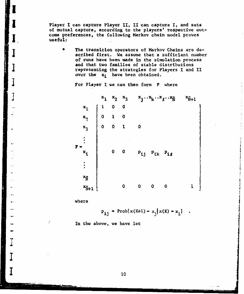
SI Player I can capture Player I1, 11 can capture I, and setsof mutual capture, according to the players' respective out-come preferences, the following Markov chain model provesuseful:

* IThe transition operators of Markov Chains are de-scribed first. We assume that a sufficient numberof runs have been made in the simulation processand that two families of stable distributionsrepresenting the strategies for Players I and IIovcr the x, have been obtained.

For Player I we can then form P where

,_- ,c x2x ,.

x1 x2 x3 xj xkI'A.xA 'R+1

xI 1 0 0

x9 0 1 0

S.3 0 0 1 0

Pm

Xi 0 0 Pij Pik Pil

XA+1 0 0 0 0 1

where j

"Pjj " Prob[x(K+l) x•I(K) - xi]

In the above, we have let

10

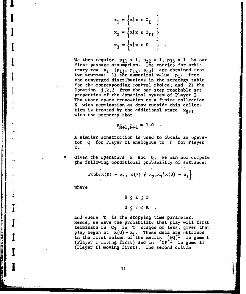
.......,.......£ ii {XI E }

= 1 - {xlx e Ci

x 3 - JXx xES

We then require Pll 1 1, P22 1 1, P33 - 1 by ourfirst passage assumption. The entries for arbi-trary row xi (PiA; Pik' Pij) are obtained fromtwo sources: ) te numerical value Pij fromthe converged distributions in the strategy tablefor the corresponding control choice; and 2) thelocation J,k,.f from the one-step reachable setproperties of the dynamical system of Player 1.The state space truncation to a finite collectionN with termination as draw outside this collec-tion is treated by the additional state xq+Iwith the property that

PN+lN+I "= 1.0

A similar construction is used to obtain an opera-tor Q for Player II analogous to P for PlayerI.

Given the operators P and Q, we can now computethe following conditional probability of entrance:

Problx (K) - xi, -() 0X3 xo i

where

"0 < K<T

I 0O5v<K ,

and where T is the stopping time parameter.Hence, we hiave the probability that play will firstterminate in C1 in T stages or less, given thatplay began at x(0)- xi. These data are obtainedin the first column of the matrix [pQ]T in game I(Player I moving first) and in [Qp]T in game II(Player 11 moving first). The second column

! ~11 i--- I

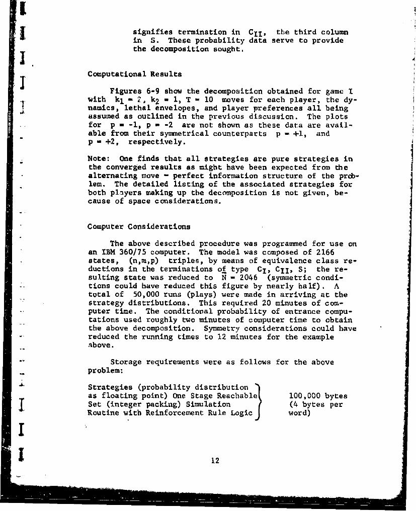
signifies termination in C11 , the third columnin S. These probability data serve to providethe decomposition sought.

Computational Results

Figures 6-9 show the decomposition obtained for game Iwith kl - • k 2 - 1 T- 10 moves for each player, the dy-

1' namics, let~hal envelopes, and player preferences all beingassumed as outlined in the previous discussion. The plotsfor p - -1, p - -2 are not shown as these data are avail-able from their symmetrical counterparts p - +1, andp - +2, respectively.

Note: One finds that all strategies are pure strategies inthe converged results as might have been expected from thealternating move - perfect information structure of the prdb-lem. The detailed listing of the associated strategies forboth players making up the decomposition is not given, be-cause of space considerations.

Computer Considerations

The above described procedure was programmed for use onan IBM 360/75 computer. The model was composed of 2166states, (nm,p) triples, by means of equivalence class re-ductions in the terminations of type CI, CII, S; the re-sulting state was reduced to N - 2046 (symmetric condi-tions could have reduced this figure by nearly half). Atotal of 50,000 runs (plays) were made in arriving at thestrategy distributions. This required 20 minutes of com-puter time. The conditional probability of entrance compu-tations used roughly two minutes of computer time to obtainthe above decomposition. Symmetry considerations could havereduced the running times to 12 minutes for the exampleabove.

Storage requirements were as follows for the above

problem:

Strategies (probability distribution

as floating point) One Stage Reachable 100,000 bytesSet (integer packing) Simulation ( (4 bytes perRoutine with Reinforcement Rule Logic J word)

12

!

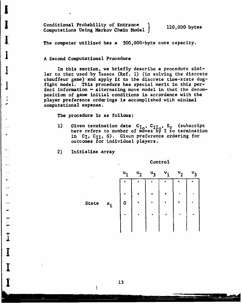
j Conditional Probability of Entrance 120,000 bytesComputations Using Markov Chain Model J

. The computer utilized has a 500,000-byte core capacity.

I A Second Computational Procedure

In this section, we briefly describe a procedure simi-lar to that used by Isaacs (Ref. 1) (in solving the discretechauffeur game) and apply it to the discrete time-state dog-

1 fight model. This protedure has special merit in this per-fect information - alternating move model in that the decom-position of game initial conditions in accordance with theplayer preference orderings is accomplished wiLh minimalcomputational expense.

The procedure is as follows:

1) Given termination data CIO, CI1 0 , So (subscripthere refers to number of moves by I to termination

"-- in CI, CII, S). Given preference ordering foroutcomes for individual players.

"2) Initialize array

Control

u 1 U 2 u3 v 1 v 2 v3

* 0 0 0 0

State xi 0

II 13

3) Select x dC I UC 1 US 0

a) for u if x ------ C1 0

set xisu 1 - 1.0 in array

1U

if xi---x C• C0

set xI- 0 in array

u 1

if i Ul x e D0

set x - 0.3 in array

u 1

i f x i.

set xi~u1 - 0.7 in array

b) Do a) over all uj

c) For xi

"(1) if 3 at least one u4 - 1.0 in arrayfor that row call xi C C1

(2) if R no u - 1.0 and at lear oneuj - 0.7 xiJ is not labeled

I

I 14

(3) if 3 no uj-1.0, and no u- 0.7.and at least one uj 0.3 call

(4) if 3 no uj - 1.0, and no uj 0.7,

#an no uj 0.3 call x C

4) Do step 3) over predetermined range ofx i CI U Cl U SO

0 0

5) Select xk i CI U C II u so UUCI U C1 1 U S1

if x, E C11 1C1 1 set xk, uI - 0 go to 5 d)

if xs I S U S1 set Xk, u1 - 0.3 go to 5 d)

a) For ul,vI: if x-k -x•i m

(1) if xm C I U C Is 0

• set xe,vI - 0 in array

(2) if x C C 1 U C II0 1

set x,,vl I in array

"(3) if X E SO SI

set x,,vI - 0.3 in array

(4) if X E D

set x2 ,v1 - 0.7 in array

b) Do a) over vj

1.5

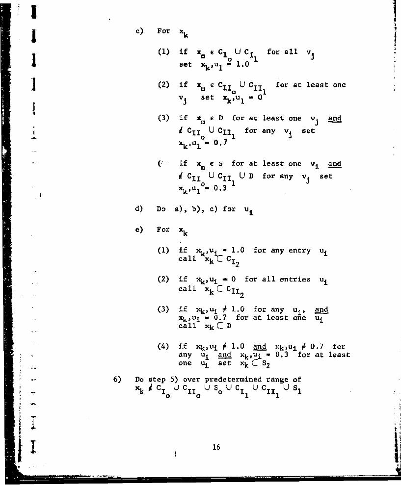
c) For xk

(1) if x e C U C for all vj

set x3,uI - 1.0

(2) if xm e Cii U C1 I for at least one

vj set xk,uI s 0

(3) if x e D for at least one v and

d, C 1 U CII1 for any vj setxkU 1 0.7

( I: if xm e 6 for at least one vi and

SC 11 U CII U D for any vj set

xk,Ul°m 0.3

d) Do a), b), c) for uS

e) For xk

(1) if xk,ui - 1.0 for any entry uicall xk C C12

(2) if xk,ui - 0 for all entries uicall xk C Cl1 2

(3) if Xk,Ui 0 1.0 for any ui, andXk,Ui - 0.7 for at least one uicall xk C D

:-=_-_:-= "(4) if Xk,Ui 0i 1.0 an_.d Xk,Ui 0 0.7 for

any u i and Xk,Ui w 0.3 for at leastone ui set xk C S2

'=-= -- 6) Do step 5) over predetermined range of

x Ck U C U S U C u C U S

I16

]I7) The extension to 3 and more stages of play using

steps 5)and 6)is straightforward.

Note: A simultaneous move version of the discrete-timestate model presented is currently under study in the Grumman

j |Research Department. In this case, a revision of the pref-erence ordering (from that assumed here) has been made toobtain ultimately a game for which a zero-sum payoff propertyis specified. In this case, one of the players is requiredto prefer the sacrifice outcome over the draw result. A dy-namic prograimning procedure is being used to conduct thestrategy synthesis with the optimal mixed strategies in thesingle-stage subgames determined by a Brown-Robinson itera-tion procedure. This procedure was first outlined by Kopp(Ref. 5) in the context of a simpler simultaneous move dog-"fight game model.

CONTINUOUS-TIHE-DISCRETE REGION GAME MODEL

IN THE HORIZOnrAL PLANE

The Continuous-Time "Regional" State One-On-One AerialCombat Model in the Horizontal Plane

The model for combat in the horizontal plane is a logi-cal extension of the discrete model and thus permits quali--A tative comparison. Both vehicles are assumed to have con-e: stant velocity.

System Equations

The kinematic equations are similar to those given byIsaacs (Ref. 1) for the game of two cars. The equations arewritten in terms of a coordinate system centered on Player i(see Fig. 10), and are given as

VI yy• + V sin 81I

17

|l"!"I f'i'l'["'1 l'i'?'" "11""[ '1'I -17

SVm Y" •'T X - VI V cos e

SRII

w where

wPl

V and V are the speeds of Vehicles I and II, re-spectively;

0 and 4 the control variables for I and II, re-spectively (both bounded); and

R and RI are the minimum turn radii of I and II,respectively

with p - 1 x2 + y2 (Range), (z (Bearing), and 0 (relativeheading angle between VI and Vii).

Observable Data and Control Variables

Since we are interested in constructing feedback con-trols, t(p,o,e) and W(p~w,O), let us look at a proposeddecomposition of the visual sphere (or circle and rays inthis two dimensional version). Based on discussions withexperience combat piloLs, we do not believe that relativerange, bearing, or heading can be measured accurately in thedogfight encounter. Thus, the state of one aircraft withrespect to the other is imperfectly known. To model thisimperfect information, we ascertained in a cursory way whatis capable of being known and to what degree of accuracy.These discussions led t3 the partitioning of the visualsphere (or visual horizontal plane in this two dimensionalversion) as shown in Fig. 11. This partitioning is madewith the assumption that Systems I and II are representativeof aircraft in the dogfighting situation. The divisionsthemselves, such as Region 41 in Fig. 11, is meant to implythat Player I can only discern that Player II is somewhere be-tween 6000 and 12000 feet ahead and somewhere between00 and 7½0 off to his right. In the partitioning shown

I18

i ] in Fig. 11, the shaded region denotes the lethal gun enve-

. lope of I and the region In which I uses a gunsight forii lead-pursuLt tracking.. We have assumed that a lingering

I time of 0.5 seconds continuously or 1.0 cumulative secondsin the gun envelope constitutes a "kill;" this isa modifica-tion of the instantaneous "kill" property of the discreteI game. The second player is assumed to have a similar par-titioning of the space.

The partitioned state space in p and w has a thirdcoordinate, 0, which we are assuming again to be imperfect.We assume also that e is known only to lie within thevalues specified below for Regions 1-41 and that it is notdiscernible for p > 12,000 feet wherein a vehicle wouldappear at best as a black dot on the horizon. Hence, 0 isobservable within the following:

3150 < e 450 e

450 < 0 135 t2

135 < 9 225 63

225 < e 3150 e

A similar breakdown applied to Player IM. Hence, in thismodel we have

41x4164 + 11 - 175 regions in the decomposition.

We have limited the admissible controls to be finite in num-ber (i.e., * - ±1, 0, and similarly 11 - ±, 0), hence,the probabilistic feedback law would be represented by thefollowing table of state doubles Xi(R,e), where R is theregion and 0 is the relative heading angle between I and

I

11

I I

For Player I

State Prob -t+1 Prob I~ Prob 4)O1 Xl (R1=-is 0- 1),- P,

Sx2 (R1 -l, e-e2)2L- 1 2)

X 4 (R -41, e m 49i x64( -4,0=4) P164 ,+1 PI6,-I P164,0•

X1 6 5 (R -42, all e)

x 1 7 5 (R-52, all 9) P 1 75 ,+ 1 P175,-1 P1 7 5 , 0

where p,•- is the probability of choosing the control-1 when -Payer I discerns that Player II is in Region 164with respect to himself.

For Player II, we have a similar table with the states givenby the proximity of Player I with respect to Player II.

State' p-1PVob . +i Prob 00

X1 (R1 M, e-el) Pp,+I Pl,-i PI,O

1X7 5 (R 52, all 0) P1 7 5 ,+l P175,-i P175,0

The sets of capture C1, CIl, and sacrifice S cannot neces-sarily be identified in terms of p,w,0 at the outset, eventhough one may be in the envelope of the other, due to thelinger time stipulation.

I I 20

Simulation Procedure

Assume that a family of games is played with durations0 < -I!, < T2 < ,. < T (see Fig. 12). Assume that the gamebegins at •nitial conditions ý (say in Region 23 for I,corresponds to 52 for II) and has duration TI. [We selectinitial conditions close to termination for I (and II). ]

Choices of control are selected from X(R -23, e- 0i)for Player I and X(R -52, all e) for Player II. Say, fcrargumenes sake, that they are 0 - +1 and p - +1, respec-tively. The differential equations are integrated from ,

using 0 - +l and 7p - +1 until Region 23 for I or Region52 for II is exited. If either occurs (or both), the newregion for that player is consulted (say 23 - 22 for I,II continues with, 52); hence X(R - 22, 0 - 01) is con-suited for the next control decision for I which, say, is0 - 0. We continue in this way until an outcome CI, CII,S, or Ti is observed. Meanwhile, the "state-control"pairs have been temporarily stored. For

1 23, 0 - +1 ; 22, t - 0

II 52, ' - +1

As in the discrete model, the reinforcement rule is appliedto alter the distributions with respect to the temporarilystored data. We have modified the reinforcement rule to beother than multiplication of the control choice chain duringany one run by a constant and then normalizing. We have in-corporated a linear weighting that reinforces the controlchoice chain more strongly after many plays of the game,hopefully avoiding the reinforcement of a basically poorchoice of control that may have led to a successful outcomeon the part of one player because the second had not yetlearned how to play adequately. We repeat LIis procedureover many • in regions close to termination using timeparameter TI; T2 is then selected, and experiments re-peated over in regions not previously covered by experi-ments using Ti.

Note: In this model we do not have to decide whether the

game is of simultaneous or alternating move structure; thesequence of moves in time resolves itself in accordance withthe assumed decomposition among the observables and the in-tegration of the kinematic equations. It should also be

21.

_ noted that we have tined the y-axis as a reflecting barrier

arnd thereby, by sy~metry, have reduced the number of storedstates in our feedback representation, and subsequently inour simulation.

Preliminary Computational Results

The results presented for the continuous 2-0 model areby no means complete, but these results do indicate that thereinforcemetit algorithm developed for the discrete game car-

Sries over directly to the continuous one.

Region 22 (el) as shown in Fig. 13 (and designatedI simply as 22 in Fig. 11) is considered representative of a• •region close to termination. We are seeking to ascertain

* - the control policy probability distributions on the part ofboth players for encounters that begiLn therein. We are alsoseeking the probability of the various possible outcomes,C1 , CII, S, and D. We fix the converged control policiesfor Region 22 (el) and, knowi.ng the probabilistic out-

comes for play entering that region, go on to consider Re-gion 22 (e 2 ). We start play in the latter region and ter-minate play if we anter Region 22 (el), which has beenpreviously decided, or terminate by the occurrance of one ofthe possible outcomes prior to entering Region 22 (01). Wereinforce accordingly, and begin new encounters until the"control choice probability dist.:ibution becomes invariantfor Region 22 (02).

The particular parameters that were chosen in this 2-Dcontinuous model mere V1 = 1000 ft/sec, VI1 = 500 ft/sec,R, - 3000 ft, and Rl = 2500 ft. Investig.4tion of thetime that any one play from a given initial conditionlasts, before a draw is considered the outcome, resulted ina time of 100 seconds. At a relative velocity between thetwo players of 500 ft/sec this time is sufficient ior thefaster player to catch the slower if the slower is near theedge of the visual threshold, as shown in Fig. 11, andheaded in the same direc.tion.

I The primary question to whtch we addressed ourselves

was: What is the most favorable probability distributionSon the choice of control decisions for Player I when he

finds Playeir II ia Region 22 (el)? Note that even thoughII is always in Region 22 (e1) with respect to I, T is notnecessarily in the same region with respect to Player II at

I22

| i Ii I ' -

~ I. the beginning of play. We utilize 80 particular sets ofinitial conditions; these are specified as all- combinations"of p - 3600 ft, 4200 ft, 4800 ft, 5400 ft; w - 1.5°0 3.0",4.50, 6.00, and e - -446o -22.5°, 00, 22.50, 440, all ofwhich fall into Region 22 (01) of II/I (Player II withrespe~ct to Player I).

We begin by dividing the unit interval equally intoV'0 parts, with each part corresponding to one of the 80

p,xw, triples (initial conditions). Starting from a uni-form distribution on the control policies of Player I forRegion 22 (61), we select an initial condition randomly,run a game, observe the outcome, make the reinforcement ac-cordingly, and choose another initial condition; then agame is run, etc., etc. This resulted in a single distribu-tion for the region which was PLT - 1.0, PSA - 0, and

i T' PRT - 0, where PLT - probability of making a Left Turn,PSA m probability of going Straight Ahead, and PRTprobability of making a Right Turn. The results of running1000 random initial conditions chosen from the 80 allowableyielded PC 0.885, PC 0.030, PS - 0, and PD = 0.085.Many of the draw outcomel and captures by Player II occurredduring the first few hundred games. If we look at games 500through 1000, the p.1 - 0.940t p0 0020, p- 0, PD0.040, which looks very good for Mayer I. One might con-lecture that a left turn when the opponent is ahead andslightly to the right is not the best policy; but aftertracing a few of the plays through, one sees that Player Iturns left as a delaying maneuver and then right (II/I is inRegion 23 (01) or in Region 23 (02) as he turns right)since he has a closing velocity of 500 ft/sec. If he hadgone straight, Player II would have turned left and could

4 have held I in the weapons envelope as he passed II. If heturned right, Player II could have made a much sharper rightand obtained a draw. Using a different random number gener-ator for selecting the initial conditions and the controlchoices led to pcI - 0.940, PC 0.009, PS - 0 and PD =0.051, but the control policy Hor Player I converged toI PLT 0, PSA - 1.0, PRT - 0 which tends to indicate thatmaking a left turn or going straight ahead on the part ofPlayer I are equally good policies and result in a highprobability of capture. Player 11's control policy choicefor the initial condition at the end of 1000 games was vir-tually a uniform distribition in both cases, indicating thatall choices of control on his part were equally bad due tohis being beaten so many times. Other regions converged

23

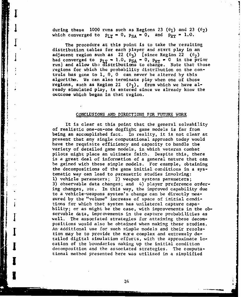
during these 1000 runs such as Regions 23 (el) and 23 (e2)which converged to PLT - 0, PSA - 0, and PRT - 1.0.

The procedure at this point is to take the resultingdistribution tables for each player and start play in anadjacent region such as 22 (e3) [since Region 22 (62)had converged to PTT 1.0, PSA - 0, PRT - 0 in the priorrun] and allow the Histributions to change. Note that those

regions for which the probability distribution on the con-trols has gone to 1, 0, 0 can never be altered by thisalgorithm. We can also terminate play when one of thoseregions, such as Region 22 (81), from which we have al-ready simulated play, is entered since we already know the

outcome which began in that region.

CONCLUSIONS AND DIRECTIONS FOR FUTURE WORK

It is clear at this point that the general solvabilityof realistic one-on-one dogfight game models is far frombeing an accomplished fact. In reality, it is not clear atpresent that any single computational approach today wouldhave the requisite efficiency and capacity to handle thevariety of detailed game models, in which veteran combatpilots might place an ultimate faith. Despite this, thereis a great deal of information of a general nature that canbe gained with these simple models. For example, obtainingthe decompositions of the game initial conditions in a sys-tematic way can lead to parametric studies involving:

*1 1) vehicle parameters; 2) weapon systems parameters;3) observable data changes; and 4) player preference order-"ing changes, 2tc. In this way, the improved capability dueto a vehicle-weapons system's change can be directly mea-sured by the "volume" increase of space of initial condi-I tions for which that system has unilateral capture capa-bility; or as might be the case, with improvements in the ob-servable data, improvements in the capture probabilities aswell. The associated strategies for attaining these decom-positions would also be obtained when making these studies.An additional use for such simple models and their resolu-tion may be to provide the mare complex and extremely de-tailed digital simulation efforts, with the approximate lo-ll cation of the boundaries making up the initial conditiondecomposition and the associated strategies. The computa-tional method presented here was utilized in a simplified

224

1 form and although the results sought were obtained, the al-gorithm as applied in these garde models is computationallyinefficient. Efforts are underway to devise better sam-pling procedures and more sophisticated reinforcement learn-ing rules in these models.

2• I| 25

IT

REFERENCE S

1 1. Isaacs, R., Differential Games, Wiley, New York, 1965.

2. Baron, S. et al., "A New Approach to Aerial CombatGames," 1NASA CR-1626, October 1970.

3. Baron, S. et al., A Study of the Markov Game Approachto Tactical Maneuvering Problems, Report No. 2179,Bolt, Beranek, and Newman, Inc., October 1971.

4. Falco, M., An Algorifhm for Strategy Synthesis inAerial Dogfight Game Models, Grumman Aerospace Corpora-tion Research Proposal RP-396, February 1971(Proprietary).

5. Kopp, R. E., The Numerical Solution of DiscreteDynamic Combat Games, RM-523J, November 1971. Pre-sented at the 4th Inter. Fed. for Info. ProcessingColl. on Optimization Techniques, Santa Monica,California, October 17-22, 1971.

6. Starr, A. W., "Nonzero-Sum Differential Games: Con-cepts and Models," Harvard University Division of

i "Engineering and Applied Physics Technical Report 590,

June 1969.

An additional reference and excellent bibliographic sourceon the topic of differential games and its applications is:

Ciletti, M. D. and Starr, A. W., Differential Games:A-Critical View, Differential Games: Theory and

"* -Applications (Symposium Proceedings of the AACC TheoryCommittee), ASME, June 1970.

I

I

26III

[ 12

ENVELOPE A I

Fig. 1 Lethal Envelope Player I

V v ENVELOPE A1

Fig. 2 Lethal Envelope Player 11

P=O Heading of I I

P=+1

P -2 P=+ 2

HEADING OF Ip=3

1 (-3)Fig. 3 Relative Heading

27

C~C9

'-W

41

0

I--o

0 C

280

III

II

m 0n,9II

M.-.8

M=O

m--188

"m 0

Fig. 5 Truncation of Region of Play

I '

29

(DI.0 PDPII 1

(O 0 0

P()1101PD)1P( 1

Figure 6. Decomposition of Starting Conditions for All N, M, with P=O

1 30

I o

P. (D)- 1.

-4P I (D) 1.0

F ~igure 7. Decomimsit im ()I Wa;rt injy C(Wdmilions foi- Al] N, MYT with P +1

10

D 0

0 j)

>I

T Figure 8. Decomposition of Starting Conditions for All N, M. with P +42

:32

(PDP(S

'33

I vI' I

1i

I

P- II

I

I Fig. 10 Coordinates for Gamne in Horizontal Plane

Ii'

- 34

1~48K24K

~~42

I412 5

41404I3

6K 2233

2 2521 35O4

I

41 40I39

id

Fig. 12 Game Play in the Horizontal Plane

1 36

315

~3 7