Keynesian Theory of Consumption. Theoretical and Practical Aspects

Kirill Breido, Ilona V. Tregub

The Finance University Under The Government Of The Russian Federation International Finance Faculty, Moscow, Russia

E-mail: ilonavl_fa@mail.ru, Fax: (495) 366 56 33

THEORETICAL ASPECTS

Recall that real GDP can be decomposed into four component parts: aggregate expenditures on

consumption, investment, government, and net exports. The income-expenditure model

considers the relationship between these expenditures and current real national income.

Aggregate expenditures on investment, I, government, G, and net exports, NX, are typically

regarded as autonomous or independent of current income. The exception is aggregate

expenditures on consumption. Keynes argues that aggregate consumption expenditures are

determined primarily by current real national income. He suggests that aggregate consumption

expenditures can be summarized by the equation

 

where C denotes autonomous consumption expenditure and Y is the level of current real income,

which is equivalent to the value of current real GDP. The marginal propensity to consume (mpc),

which multiplies Y, is the fraction of a change in real income that is currently consumed. In most

economies, the mpc is quite high, ranging anywhere from .60 to .95. Note that as the level of Y

increases, so too does the level of aggregate consumption.

Total aggregate expenditure, AE, can be written as the equation

where A denotes total autonomous expenditure, or the sum C + I + G + NX. Different levels of

autonomous expenditure, A, and real national income, Y, correspond to different levels of

aggregate expenditure, AE.

Equilibrium real GDP in the income-expenditure model is found by setting current real national

income, Y, equal to current aggregate expenditure, AE. Algebraically, the equilibrium condition

that Y = AE implies that

2  

1

where

In words, the equilibrium level of real GDP, Y*, is equal to the level of autonomous expenditure,

A, multiplied by m, the Keynesian multiplier. Because the mpc is the fraction of a change in real

national income that is consumed, it always takes on values between 0 and 1. Consequently, the

Keynesian multiplier, m, is always greater than 1, implying that equilibrium real GDP, Y*, is

always a multiple of autonomous aggregate expenditure, A, which explains why m is referred to

as the Keynesian multiplier.

PRACTICAL ASPECTS

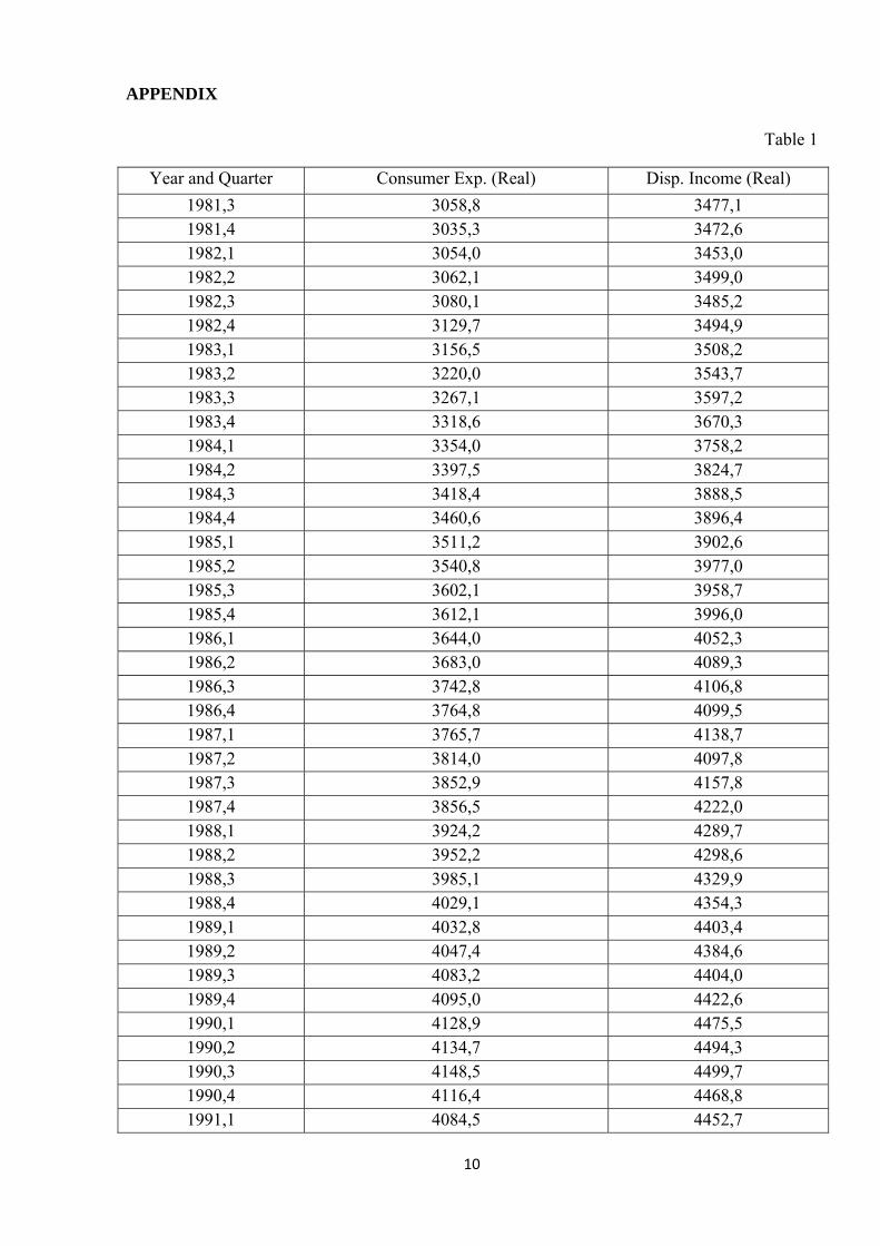
DATA

As soon as we analyze and test the Keynesian economic consumption, we should find out some

specific data, i.e. real consumer expenditures, adjusted to inflation (mlns of current US$), which

we will denote yt, and real disposable income, also adjusted to inflation (mlns of current US$),

which we will denote as xt. But we also need long-term time series of economic data of a

particular country. Let us observe and test the simplest example - economy of the USA.

We will take quarterly data from the 3 quarter of 1961 to 2 quarter of 1996. We will leave the

corresponding data for the 3 quarter of 1996 for model forecasting.

So, we should collect appropriate numbers to estimate the model. The data has been collected at

http://www.economicswebinstitute.org, Economics Web Institute, and

http://www.wwnorton.com/college/econ/macro/, Hall and Taylor "Macroeconomics" page.

(Appendix, Table 1.)

MODEL TESTING

Model Specification

Here is the mathematical interpretation for our economic model - the Keynesian Consumrtion

function.

0  

3  

It includes all the variables needed: Yt – real consumer expenditures, adjusted to inflation (mlns

of current US$) in the US economy, Xt – real disposable income, also adjusted to inflation (mlns

of current US$) in the US economy, β0 – Autonomous consumption, β1 – the marginal propensity

to consume, plus the disturbance term for different “noises”.

Steps explanation and results interpretation

We need to put into the rows of Regression, Data Analysis the corresponding data of endogenous

and exogenous variables from the 3 quarter of 1961 to 2 quarter of 1996.

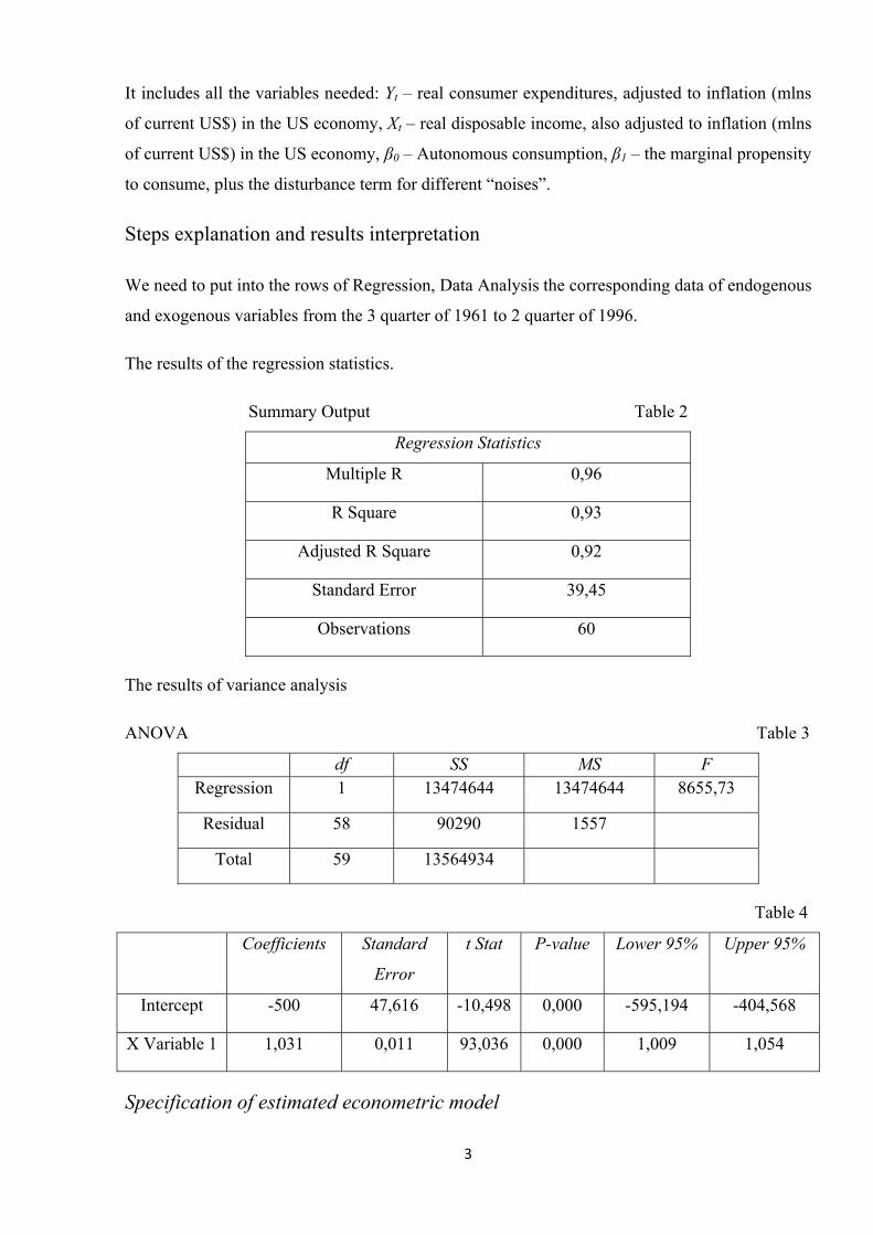
The results of the regression statistics.

Summary Output Table 2

Regression Statistics

Multiple R 0,96

R Square 0,93

Adjusted R Square 0,92

Standard Error 39,45

Observations 60

The results of variance analysis

ANOVA Table 3

df SS MS F Regression 1 13474644 13474644 8655,73

Residual 58 90290 1557

Total 59 13564934

Table 4

Coefficients Standard

Error

t Stat P-value Lower 95% Upper 95%

Intercept -500 47,616 -10,498 0,000 -595,194 -404,568

X Variable 1 1,031 0,011 93,036 0,000 1,009 1,054

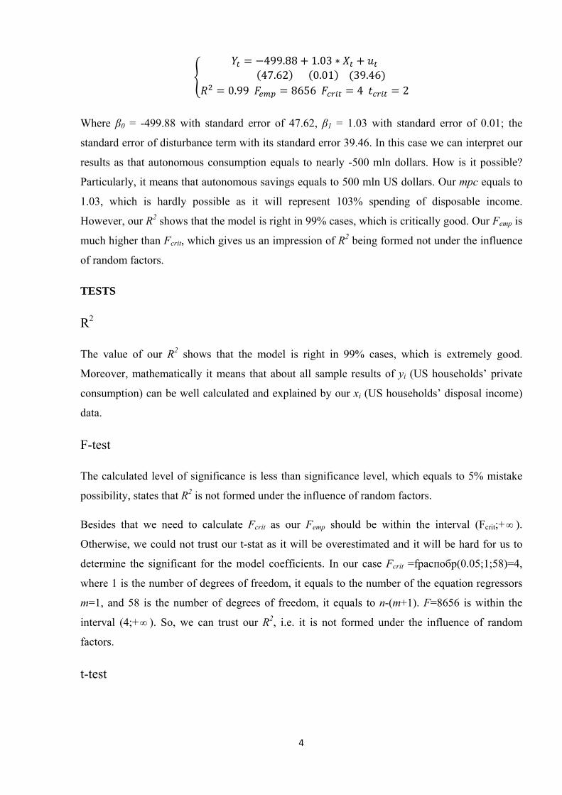
Specification of estimated econometric model

4  

499.88 1.03 47.62 0.01 39.460.99 8656 4 2

Where β0 = -499.88 with standard error of 47.62, β1 = 1.03 with standard error of 0.01; the

standard error of disturbance term with its standard error 39.46. In this case we can interpret our

results as that autonomous consumption equals to nearly -500 mln dollars. How is it possible?

Particularly, it means that autonomous savings equals to 500 mln US dollars. Our mpc equals to

1.03, which is hardly possible as it will represent 103% spending of disposable income.

However, our R2 shows that the model is right in 99% cases, which is critically good. Our Femp is

much higher than Fcrit, which gives us an impression of R2 being formed not under the influence

of random factors.

TESTS

R2

The value of our R2 shows that the model is right in 99% cases, which is extremely good.

Moreover, mathematically it means that about all sample results of yi (US households’ private

consumption) can be well calculated and explained by our xi (US households’ disposal income)

data.

F-test

The calculated level of significance is less than significance level, which equals to 5% mistake

possibility, states that R2 is not formed under the influence of random factors.

Besides that we need to calculate Fcrit as our Femp should be within the interval (Fcrit;+∞ ).

Otherwise, we could not trust our t-stat as it will be overestimated and it will be hard for us to

determine the significant for the model coefficients. In our case Fcrit =fраспобр(0.05;1;58)=4,

where 1 is the number of degrees of freedom, it equals to the number of the equation regressors

m=1, and 58 is the number of degrees of freedom, it equals to n-(m+1). F=8656 is within the

interval (4;+ ). So, we can trust our R2, i.e. it is not formed under the influence of random

factors.

∞

t-test

5  

|

⁄

1/

st

T-test itself shows which coefficients are significant and which are not, that is | . For

this purpose we need to calculate tcrit. tcrit= 3.57. In our case all absolute values of t-stat are more

than tcrit, therefore, all the regression coefficients are significant.

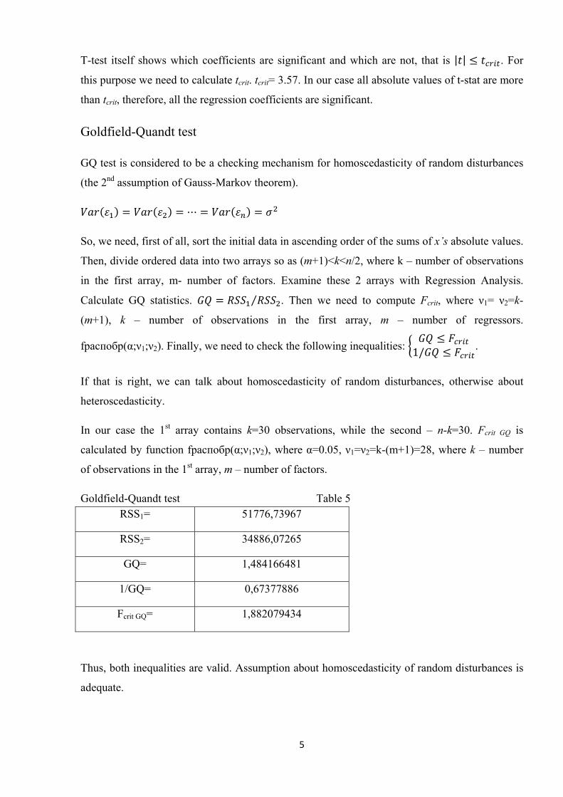
Goldfield-Quandt test

GQ test is considered to be a checking mechanism for homoscedasticity of random disturbances

(the 2nd assumption of Gauss-Markov theorem).

So, we need, first of all, sort the initial data in ascending order of the sums of x’s absolute values.

Then, divide ordered data into two arrays so as (m+1)<k<n/2, where k – number of observations

in the first array, m- number of factors. Examine these 2 arrays with Regression Analysis.

Calculate GQ statistics. . Then we need to compute Fcrit, where ν1= ν2=k-

(m+1), k – number of observations in the first array, m – number of regressors.

fраспобр(α;ν1;ν2). Finally, we need to check the following inequalities: .

If that is right, we can talk about homoscedasticity of random disturbances, otherwise about

heteroscedasticity.

In our case the 1 array contains k=30 observations, while the second – n-k=30. Fcrit GQ is

calculated by function fраспобр(α;ν1;ν2), where α=0.05, ν1=ν2=k-(m+1)=28, where k – number

of observations in the 1st array, m – number of factors.

Goldfield-Quandt test Table 5 RSS = 51776,73967 1

RSS2= 34886,07265

GQ= 1,484166481

1/GQ= 0,67377886

Fcrit GQ= 1,882079434

Thus, both inequalities are valid. Assumption about homoscedasticity of random disturbances is

adequate.

6  

, 0 1

∑ ∑⁄

0; ; 4 ; 4

0; ; 4 ; 4

; ; 4 ; 4

Autocorrelation normally occurs only in regression analysis using time-series data. The

If there exists residuals’ autocorrelation, we need to include lagging factor so as to avoid the

t-1

i(t-1)

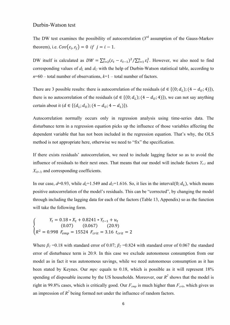
In our case, d=0.93, while dL=1.549 and dU=1.616. So, it lies in the interval 0; , which means

0.18 0.8241 0.07 0.067 20.9

0.998 15524 3.16 2

Where β1 =0.18 with standard error of 0.07; β2 =0.824 with standard error of 0.067 the standard

an impression of R2 being formed not under the influence of random factors.

Durbin-Watson test

The DW test examines the possibility of autocorrelation (3rd assumption of the Gauss-Markov

theorem), i.e. .

DW itself is calculated as . However, we also need to find

corresponding values of dL and dU with the help of Durbin-Watson statistical table, according to

n=60 – total number of observations, k=1 – total number of factors.

There are 3 possible results: there is autocorrelation of the residuals ( ),

there is no autocorrelation of the residuals ( ), we can not say anything

certain about it ( ).

disturbance term in a regression equation picks up the influence of those variables affecting the

dependent variable that has not been included in the regression equation. That’s why, the OLS

method is not appropriate here, otherwise we need to “fix” the specification.

influence of residuals to their next ones. That means that our model will include factors Y and

X and corresponding coefficients.

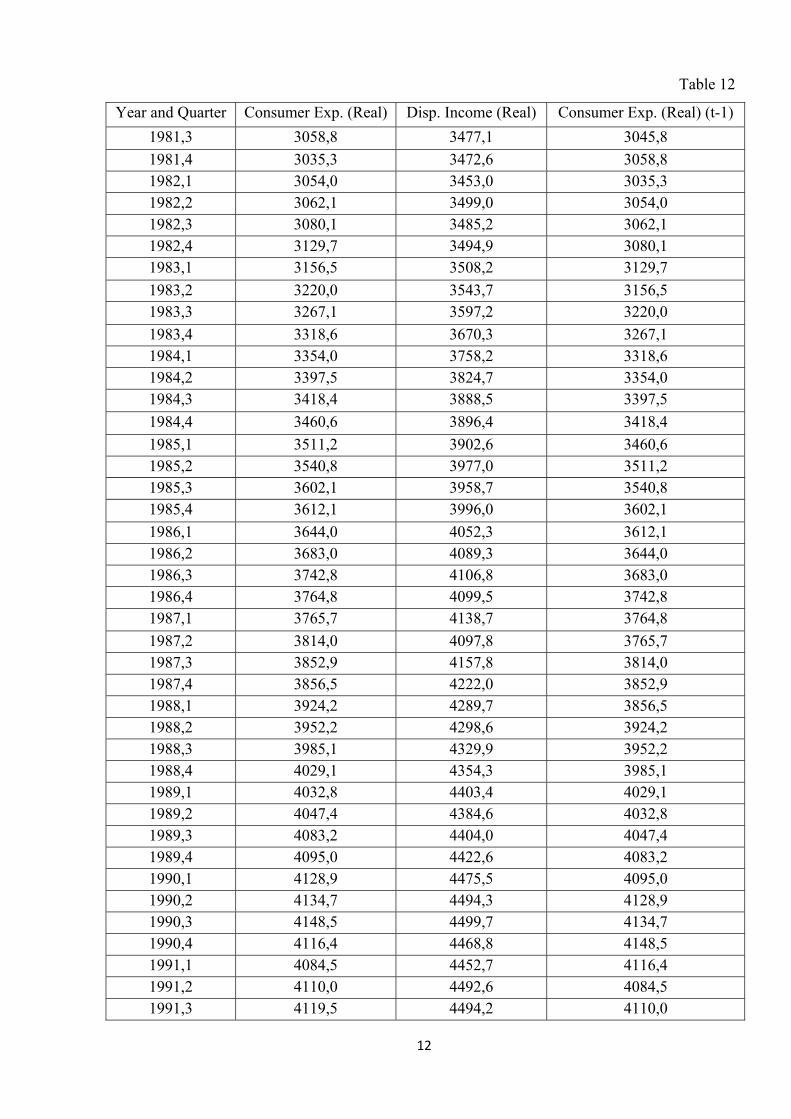
positive autocorrelation of the model’s residuals. This can be “corrected”, by changing the model

through including the lagging data for each of the factors (Table 13, Appendix) so as the function

will take the following form.

error of disturbance term is 20.9. In this case we exclude autonomous consumption from our

model as in fact it was autonomous savings, while we need autonomous consumption as it has

been stated by Keynes. Our mpc equals to 0.18, which is possible as it will represent 18%

spending of disposable income by the US households. Moreover, our R2 shows that the model is

right in 99.8% cases, which is critically good. Our Femp is much higher than Fcrit, which gives us

7  

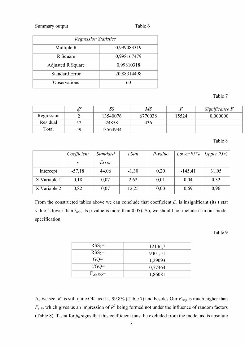
Summary output Table 6

Regression Statistics

Multiple R 0,999083319

R Square 0,998167479

Adjusted R Square 0,99810318

Standard Error 20,88314498

Observations 60

Table 7

df SS MS F Significance F Regression 2 13540076 6770038 15524 0,000000 Residual 57 24858 436

Total 13564934 59

Table 8

Coe nt

s

Sta

Error

t Stat P-value Lower 95% Upper 95%fficie ndard

Intercept -57,18 44,06 -1,30 0,20 -145,41 31,05

X Variable 1 0,18 0,07 2,62 0,01 0,04 0,32

X Variable 2 0,82 0,69 0,96 0,07 12,25 0,00

From the construct les abo can con that co nt β0 is insignificant (its t stat

than ts p-valu ore than 0.05). So, w ld not i it in ou el

specification.

RSS1= 12136,7

ed tab ve we clude efficie

value is lower tcrit; i e is m e shou nclude r mod

Table 9

RSS2= 9401,51 GQ= 1,29093

1/GQ= 0,77464 Fcrit GQ= 1,86081

As we see, R2 is still quite OK, as it is 99.8% (Table 7) and besides Our Femp is much higher than

crit, which gives us an impression of R2 being formed not under the influence of random factors

(Table 8). T-stat for β0 signs that this coefficient must be excluded from the model as its absolute

F

8  

=

relation of the model’s residuals.

t the

future correctly using our model. For this purpose we need to check whether real data of rd quarter of 1996, which

e interval.

95% Empirical<Higher 95%

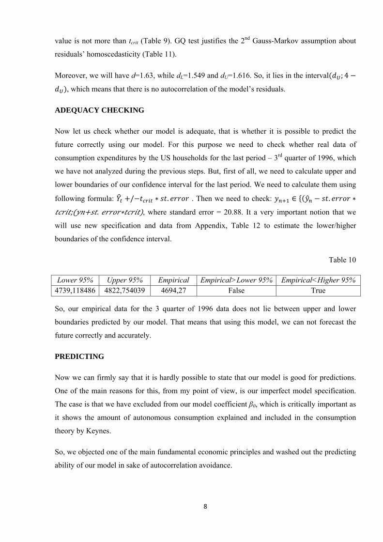
value is not more than tcrit (Table 9). GQ test justifies the 2nd Gauss-Markov assumption about

residuals’ homoscedasticity (Table 11).

Moreover, we will have d 1.63, while dL=1.549 and dU=1.616. So, it lies in the interval ; 4

, which means that there is no autocor

ADEQUACY CHECKING

Now let us check whether our model is adequate, that is whether it is possible to predic

consumption expenditures by the US households for the last period – 3

we have not analyzed during the previous steps. But, first of all, we need to calculate upper and

lower boundaries of our confidence interval for the last period. We need to calculate them using

following formula: / . . Then we need to check: .

; . , where standard error = 20.88. It a very important notion that we

will use new specification and data from Appendix, Table 12 to estimate the lower/higher

boundaries of the confidenc

Table 10

Lower 95% Upper 95% Empirical Empirical>Lower4739,118486 4822,754039 4694,27 False True

So, our empirical data for the 3 quarter of 1996 data does not lie between upper a

o ea ,

y .

s hardly possible to state that our model is good for predictions.

One of the main reasons for this, from my point of view, is our imperfect model specification.

e have excluded from our model coefficient β0, which is critically important as

nd lower

boundaries predicted by our m del. That m ns that using this model we can not forecast the

future correctl and accurately

PREDICTING

Now we can firmly say that it i

The case is that w

it shows the amount of autonomous consumption explained and included in the consumption

theory by Keynes.

So, we objected one of the main fundamental economic principles and washed out the predicting

ability of our model in sake of autocorrelation avoidance.

9  

Analyzing everything written above we can conclude that our model accepts 2nd and 3rd Gauss-

arkov assumptions about residuals’’ homoscedasticity and zero autocorrelation,

correspondently. Moreover, we have finally determined the Marginal Propensity to Consume for

18% of their disposable income.

So, our model is of a not satisfactory explanatory ability of real time-series data, such as

CONCLUSION

M

the US households, which equals to

Nevertheless, we rejected the autonomous consumption (coefficient β0) and, consequently, this

factor is omitted. More than that, we found out that we cannot predict the future correctly. That

is why, from macroeconomic point of view, our model is incorrect.

households’ private consumption in the USA predicting and cannot be used for general data

analysis of consumption functions.

10  

PPENDIX

Table 1

Year and Quarter Consumer Exp. (Real) Disp. Income (Real)

A

1981,3 3058,8 3477,1 1981,4 3035,3 3472,6 1982,1 3054,0 3453,0 1982,2 3062,1 3499,0 1982,3 3080,1 3485,2 1982,4 3129,7 3494,9 1983,1 3156,5 3508,2 1983,2 3220,0 3543,7 1983,3 3267,1 3597,2 1983,4 3318,6 3670,3 1984,1 3354,0 3758,2 1984,2 3397,5 3824,7 1984,3 3418,4 3888,5 1984,4 3460,6 3896,4 1985,1 3511,2 3902,6 1985,2 3540,8 3977,0 1985,3 3602,1 3958,7 1985,4 3612,1 3996,0 1986,1 3644,0 4052,3 1986,2 3683,0 4089,3 1986,3 3742,8 4106,8 1986,4 3764,8 4099,5 1987,1 3765,7 4138,7 1987,2 3814,0 4097,8 1987,3 3852,9 4157,8 1987,4 3856,5 4222,0 1988,1 3924,2 4289,7 1988,2 3952,2 4298,6 1988,3 3985,1 4329,9 1988,4 4029,1 4354,3 1989,1 4032,8 4403,4 1989,2 4047,4 4384,6 1989,3 4083,2 4404,0 1989,4 4095,0 4422,6 1990,1 4128,9 4475,5 1990,2 4134,7 4494,3 1990,3 4148,5 4499,7 1990,4 4116,4 4468,8 1991,1 4084,5 4452,7

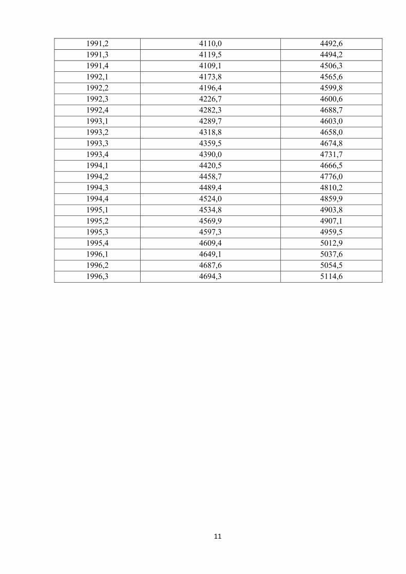
11  

1991,2 4110,0 4492,6 1991,3 4119,5 4494,2 1991,4 4109,1 4506,3 1992,1 4173,8 4565,6 1992,2 4196,4 4599,8 1992,3 4226,7 4600,6 1992,4 4282,3 4688,7 1993,1 4289,7 4603,0 1993,2 4318,8 4658,0 1993,3 4359,5 4674,8 1993,4 4390,0 4731,7 1994,1 4420,5 4666,5 1994,2 4458,7 4776,0 1994,3 4489,4 4810,2 1994,4 4524,0 4859,9 1995,1 4534,8 4903,8 1995,2 4569,9 4907,1 1995,3 4597,3 4959,5 1995,4 4609,4 5012,9 1996,1 4649,1 5037,6 1996,2 4687,6 5054,5 1996,3 4694,3 5114,6

12  

Table 12

Year and Quarter Consumer Exp. (Real) Disp. Income (Real) Consumer Exp. (Real) (t-1)

1981,3 3058,8 3477,1 3045,8 1981,4 3035,3 3472,6 3058,8 1982,1 3054,0 3453,0 3035,3 1982,2 3062,1 3499,0 3054,0 1982,3 3080,1 3485,2 3062,1 1982,4 3129,7 3494,9 3080,1 1983,1 3156,5 3508,2 3129,7 1983,2 3220,0 3543,7 3156,5 1983,3 3267,1 3597,2 3220,0 1983,4 3318,6 3670,3 3267,1 1984,1 3354,0 3758,2 3318,6 1984,2 3397,5 3824,7 3354,0 1984,3 3418,4 3888,5 3397,5 1984,4 3460,6 3896,4 3418,4 1985,1 3511,2 3902,6 3460,6 1985,2 3540,8 3977,0 3511,2 1985,3 3602,1 3958,7 3540,8 1985,4 3612,1 3996,0 3602,1 1986,1 3644,0 4052,3 3612,1 1986,2 3683,0 4089,3 3644,0 1986,3 3742,8 4106,8 3683,0 1986,4 3764,8 4099,5 3742,8 1987,1 3765,7 4138,7 3764,8 1987,2 3814,0 4097,8 3765,7 1987,3 3852,9 4157,8 3814,0 1987,4 3856,5 4222,0 3852,9 1988,1 3924,2 4289,7 3856,5 1988,2 3952,2 4298,6 3924,2 1988,3 3985,1 4329,9 3952,2 1988,4 4029,1 4354,3 3985,1 1989,1 4032,8 4403,4 4029,1 1989,2 4047,4 4384,6 4032,8 1989,3 4083,2 4404,0 4047,4 1989,4 4095,0 4422,6 4083,2 1990,1 4128,9 4475,5 4095,0 1990,2 4134,7 4494,3 4128,9 1990,3 4148,5 4499,7 4134,7 1990,4 4116,4 4468,8 4148,5 1991,1 4084,5 4452,7 4116,4 1991,2 4110,0 4492,6 4084,5 1991,3 4119,5 4494,2 4110,0

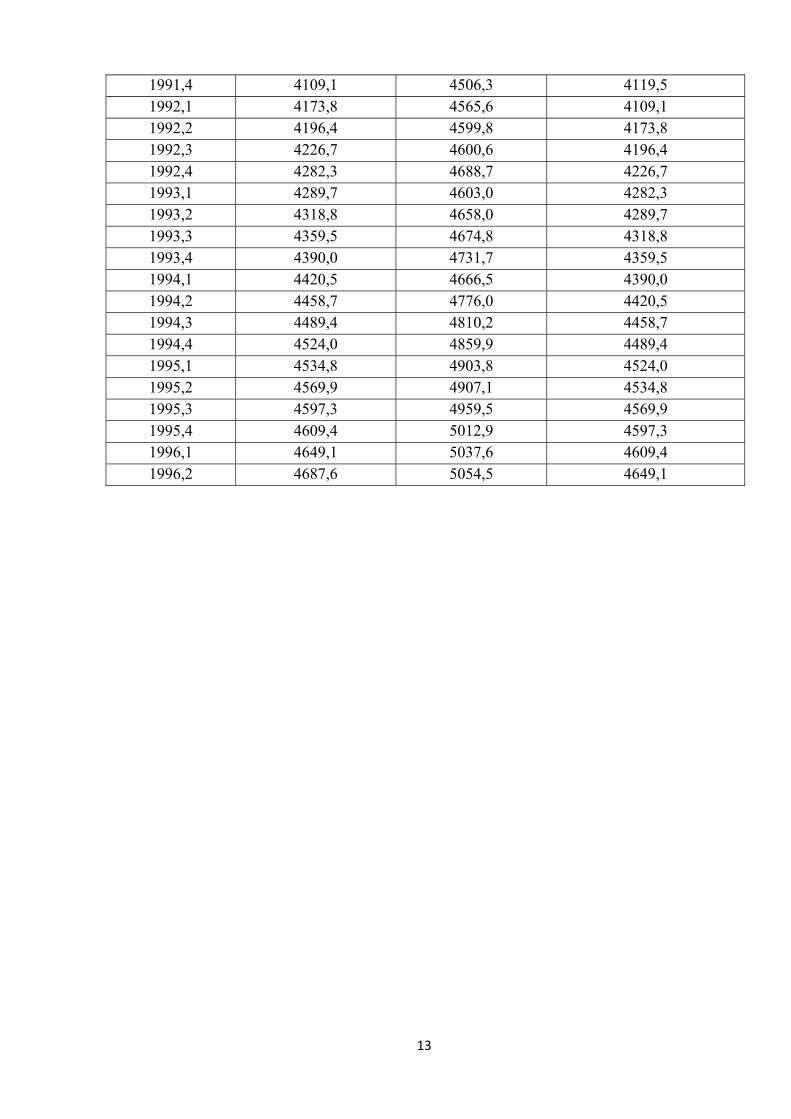
13  

1991,4 4109,1 4506,3 4119,5 1992,1 4173,8 4565,6 4109,1 1992,2 4196,4 4599,8 4173,8 1992,3 4226,7 4600,6 4196,4 1992,4 4282,3 4688,7 4226,7 1993,1 4289,7 4603,0 4282,3 1993,2 4318,8 4658,0 4289,7 1993,3 4359,5 4674,8 4318,8 1993,4 4390,0 4731,7 4359,5 1994,1 4420,5 4666,5 4390,0 1994,2 4458,7 4776,0 4420,5 1994,3 4489,4 4810,2 4458,7 1994,4 4524,0 4859,9 4489,4 1995,1 4534,8 4903,8 4524,0 1995,2 4569,9 4907,1 4534,8 1995,3 4597,3 4959,5 4569,9 1995,4 4609,4 5012,9 4597,3 1996,1 4649,1 5037,6 4609,4 1996,2 4687,6 5054,5 4649,1