Embed Size (px)
Citation preview
Key Moments in the History
of Numerical Analysis
Michele Benzi
Department of Mathematics
and Computer Science
Emory University
Atlanta, GA
http://www.mathcs.emory.edu/∼benzi
Outline
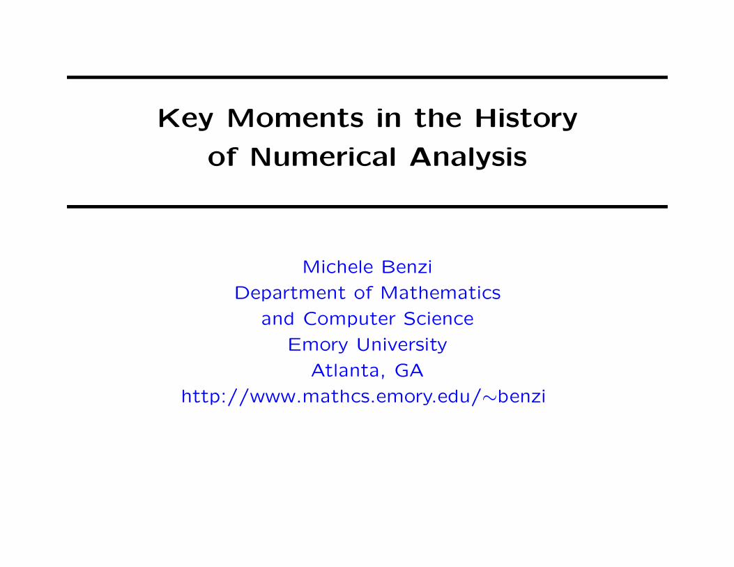
• Part I: Broad historical outline
1. The prehistory of Numerical Analysis
2. Key moments of 20th Century Numerical Analysis
• Part II: The early history of matrix iterations
1. Iterative methods prior to about 1930
2. Mauro Picone and Italian applied mathematics in
the Thirties
3. Lamberto Cesari’s work on iterative methods
4. Gianfranco Cimmino and his method
5. Cimmino’s legacy

PART I
Broad historical outline
The prehistory of Numerical Analysis
In contrast to more classical fields of mathematics, like
Analysis, Number Theory or Algebraic Geometry, Numerical
Analysis (NA) became an independent mathematical disci-
pline only in the course of the 20th Century.
This is perhaps surprising, given that effective methods of
computing approximate numerical solutions to mathematical
problems are already found in antiquity (well before Euclid!),
and were especially prevalent in ancient India and China.
While algorithmic mathematics thrived in ancient Asia, classical Greek
mathematicians showed relatively little interest in it and cultivated Ge-
ometry instead. Nevertheless, Archimedes (3rd Century BCE) was a
master calculator.
The prehistory of Numerical Analysis (cont.)
Many numerical methods studied in introductory NA courses
bear the name of great mathematicians including Newton,
Euler, Lagrange, Gauss, Jacobi, Fourier, Chebyshev, and so
forth.
However, it should be kept in mind that well into the
19th Century, the distinction between mathematics and
natural philosophy (including physics, chemistry, astronomy
etc.) was almost non-existent. Scientific specialization is a
modern phenomenon, and nearly all major mathematicians
were also physicists and astronomers.
Indeed, a look at the original works of these great mathematicians shows
that almost without exception, the numerical methods bearing their
names were introduced in the context of physical, astronomical or tech-
nical applications.
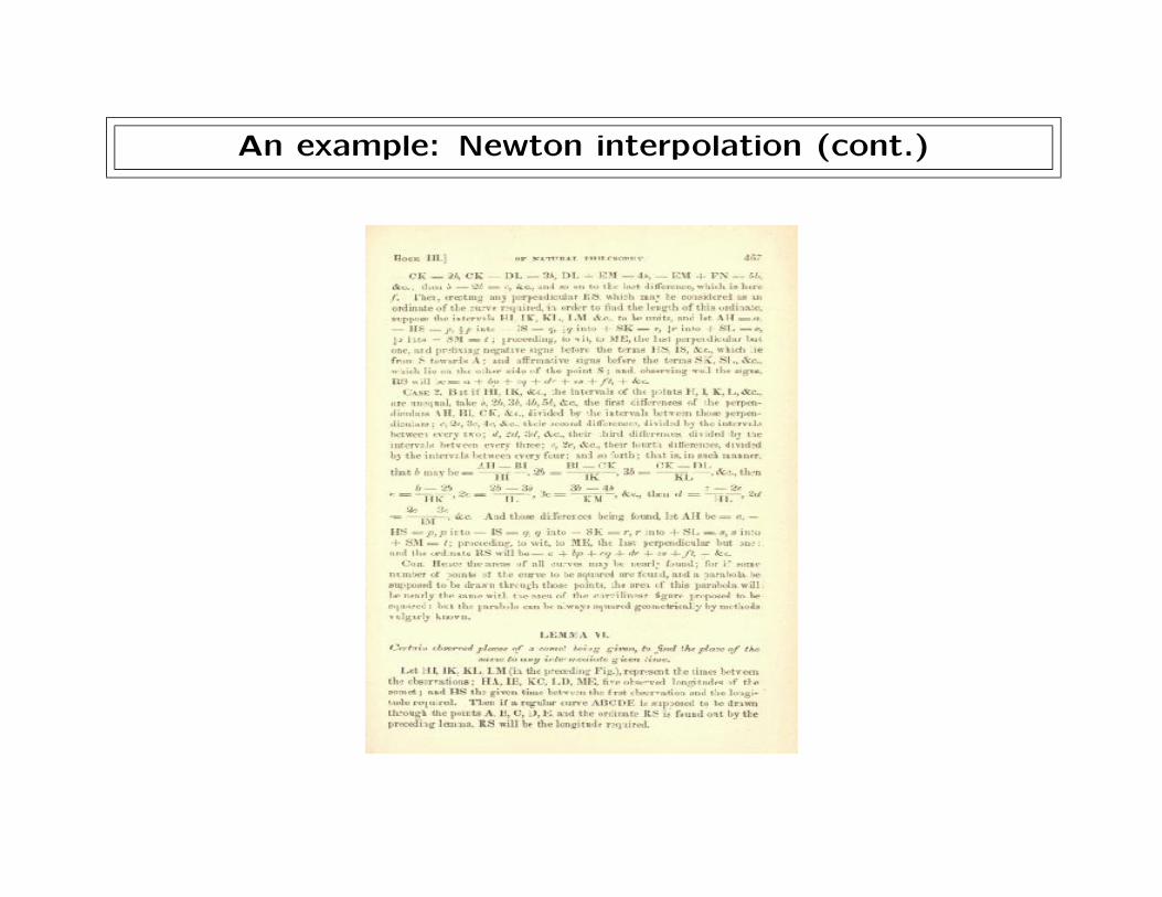
An example: Newton interpolation
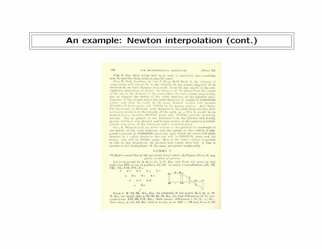
In Book III, Lemma V, of his 1687 masterpiece, Math-
ematical Principles of Natural Philosophy, Isaac Newton
(1642-1727) poses the following problem:
To find a curved line of the parabolic kind which shall pass
through any given number of points.
(Note: here parabolic = polynomial).
After solving the problem by constructing the interpolating
polynomial by divided differences, he proceeds to apply it in
the subsequent Lemma VI to the problem:
Certain observed places of a comet being given, to find the
place of the same at any intermediate given time.
An example: Newton interpolation (cont.)
An example: Newton interpolation (cont.)
The prehistory of Numerical Analysis (cont.)
Beginning with the second half of the 19th Century,
mathematician becomes almost synonymous with pure
mathematician. Most mathematics becomes conceptual
and far removed from applications. Numerical methods
are developed out of necessity to solve problems arising in
geodesy, astronomy, physics and engineering. Examples:
• In Linear Algebra we have Gauss–Jordan elimination for
Ax = b (Geodesy) and Jacobi’s methods for Ax = b and
Ax = λx (Celestial Mechanics);
• In Ordinary Differential Equations, we have the methods
of Adams and Moulton (Celestial Mechanics) and Runge–
Kutta (Aerodynamics);
• In PDEs, the Rayleigh–Ritz method (vibration problems
in Acoustics and Elasticity).
The prehistory of Numerical Analysis (cont.)
This situation persists in the first few decades of the 20th
Century. NA is not recognized as a mathematical discipline;
university professorships and courses are non-existent,
textbooks are scarce, and computing machines are primitive.
Early books on numerical methods are:
1. E. T. Whittaker and G. Robinson, The Calculus of Obser-
vations. A Treatise on Numerical Mathematics, London,
1924.
2. G. Cassinis, Calcoli Numerici, Grafici e Meccanici, Pisa,
1928.
3. J. B. Scarborough, Numerical Mathematical Analysis,
Baltimore, 1930.
These books are mostly aimed at scientists and engineers.
The prehistory of Numerical Analysis (cont.)
It should be kept in mind that before the invention of
electronic digital computers (mid-1940s), computations
were done by hand, by slide ruler, by desk calculators and,
in the first part of the 20th Century, by electro-mechanical
and analogical devices.
Two excellent references on the early history of NA and
Computing are:
H. H. Goldstine, A History of Numerical Analysis from the
15th Through the 19th Century, Springer, New York, 1977.
H. H. Goldstine, The Computer from Pascal to von Neumann,
Princeton University Press, Princeton, NJ, 1972.
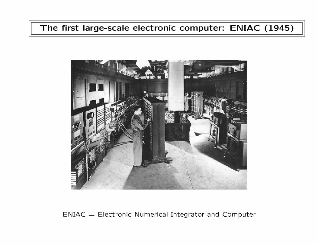
The first large-scale electronic computer: ENIAC (1945)
ENIAC = Electronic Numerical Integrator and Computer
Key Moments of 20th Century Numerical Analysis
Modern NA begins in the 1940s, as a result of two related
events: the participation of large numbers of mathemati-
cians in the war effort (especially in USA, Germany, USSR),
and the development of the first digital electronic computers.
However, some important pre-war developments should be
mentioned here:
• The analysis of finite difference methods for PDEs:
Richardson (1910); Phillips and Wiener (1923); Courant,
Friedrichs and Lewy (1928).
• The emergence of a school of applied mathematics
in Germany, mostly through the efforts of Felix Klein
(Gottingen: Runge, Courant; Berlin: von Mises).
• The creation, in Italy, of the first research institute en-
tirely devoted to NA (Picone, late 1920s).
Key Moments of 20th Century NA (cont.)
In the States, very little work in Applied Mathematics
was done prior to the late 1930s. The situation changed
dramatically as a result of the influx of European refugees,
especially from Nazi Germany, beginning in 1933. Many of
these scientists were to give a major contribution to the war
effort.
The pre-eminent figure here is perhaps Richard Courant
(1888–1972), who was the successor of David Hilbert
(1862–1943) as the director of the famous Mathematical
Institute in Gottingen.
In the period 1900–1930, the University of Gottingen had established
itself as one of the great centers for research in mathematics and physics
worldwide. During the 19th Century, the mathematics faculty included
Gauss, Dirichlet, Riemann and Klein. In the 1920s, Gottingen became a
leading center for research in quantum physics.
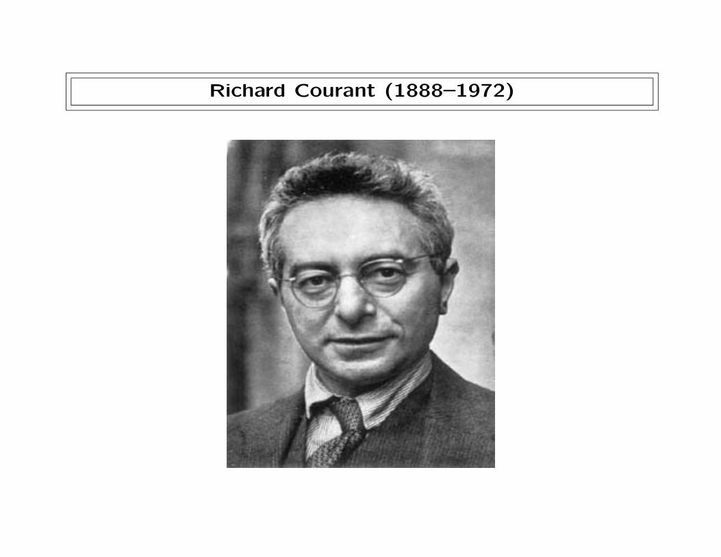
Richard Courant (1888–1972)
Key Moments of 20th Century NA (cont.)
Two famous papers on finite differences:
L. F. Richardson, The approximate arithmetical solution by
finite differences of physical problems involving differential
equations with an application to stresses in a masonry dam,
Philosophical Transactions of the Royal Society of London,
A, 210 (1910), pp. 307–357.
R. Courant, K. O. Friedrichs, and H. Lewy, Uber die partiellen
Differenzengleichungen der mathematischen Physik, Mathe-
matische Annalen 100 (1928), pp. 32–74. Translated by
Phyllis Fox as: On the partial difference equations of mathe-
matical physics, IBM Journal of Research and Development,
11 (1967), pp. 215–234. With a commentary by P. D. Lax.
Key Moments of 20th Century NA (cont.)
The celebrated CFL paper used finite differences not to
solve practical problems, but to establish existence and
uniqueness results for elliptic boundary value and eigenvalue
problems, and for the initial value problem for hyperbolic
and parabolic PDEs. It also introduced for the first time the
method of random walks for approximating the solution of
PDEs.
This paper was to have enormous influence on the numerical
analysis of PDEs, especially through the work of John von
Neumann at Los Alamos at the time of the Manhattan
Project.
The paper also influenced the development by John Curtiss in the early
1950s of Monte Carlo methods for evaluating (functionals of) solutions
of PDEs.
A quote from the CFL paper
From the Introduction:
Nowhere do we assume the existence of the solution to the
differential equation problem—on the contrary, we obtain a
simple existence proof by using the limiting process. For the
case of elliptic equations convergence is obtained indepen-
dently of the choice of the mesh, but we will find that for
the case of the initial value problem for hyperbolic equations,
convergence is obtained only if the ratio of the mesh widths
in different directions satisfies certain inequalities which in
turn depend on the position of the characteristics relative to
the mesh.
A quote from the CFL paper (cont.)
From Part II, section 2:
In the same way that the solution of a linear hyperbolic equa-
tion at a point S depends only on a certain part of the initial
line—namely the “domain of dependence” lying between the
two characteristics drawn through S, the solution of the dif-
ference equation has also at the point S a certain domain of
dependence... We shall now consider a (...) general rectan-
gular mesh with mesh size equal to h (time interval) in the
t-direction and equal to kh (space interval) in the x-direction,
where k is a constant. The domain of dependence for the
difference equation (...) for this mesh will now either lie
entirely within the domain of dependence of the differential
equation, ∂2u/∂t2 − ∂2u/∂x2 = 0, or on the other hand will
contain this latter region inside its own domain according as
k < 1 or k > 1 respectively.
A quote from the CFL paper (cont.)
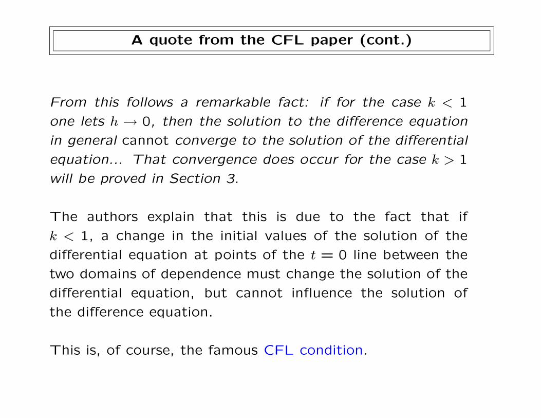
From this follows a remarkable fact: if for the case k < 1
one lets h → 0, then the solution to the difference equation
in general cannot converge to the solution of the differential
equation... That convergence does occur for the case k > 1
will be proved in Section 3.
The authors explain that this is due to the fact that if
k < 1, a change in the initial values of the solution of the
differential equation at points of the t = 0 line between the
two domains of dependence must change the solution of the
differential equation, but cannot influence the solution of
the difference equation.
This is, of course, the famous CFL condition.
Key Moments of 20th Century NA (cont.)
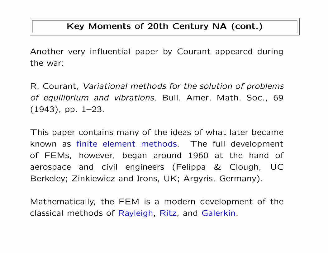
Another very influential paper by Courant appeared during
the war:
R. Courant, Variational methods for the solution of problems
of equilibrium and vibrations, Bull. Amer. Math. Soc., 69
(1943), pp. 1–23.
This paper contains many of the ideas of what later became
known as finite element methods. The full development
of FEMs, however, began around 1960 at the hand of
aerospace and civil engineers (Felippa & Clough, UC
Berkeley; Zinkiewicz and Irons, UK; Argyris, Germany).
Mathematically, the FEM is a modern development of the
classical methods of Rayleigh, Ritz, and Galerkin.
A quote from Courant’s 1943 paper
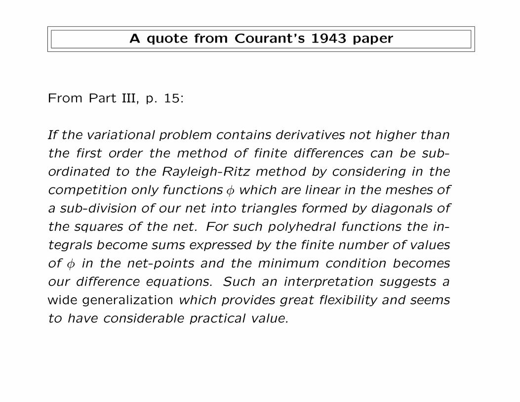
From Part III, p. 15:
If the variational problem contains derivatives not higher than
the first order the method of finite differences can be sub-
ordinated to the Rayleigh-Ritz method by considering in the
competition only functions φ which are linear in the meshes of
a sub-division of our net into triangles formed by diagonals of
the squares of the net. For such polyhedral functions the in-
tegrals become sums expressed by the finite number of values
of φ in the net-points and the minimum condition becomes
our difference equations. Such an interpretation suggests a
wide generalization which provides great flexibility and seems
to have considerable practical value.
A quote from Courant’s 1943 paper (cont.)
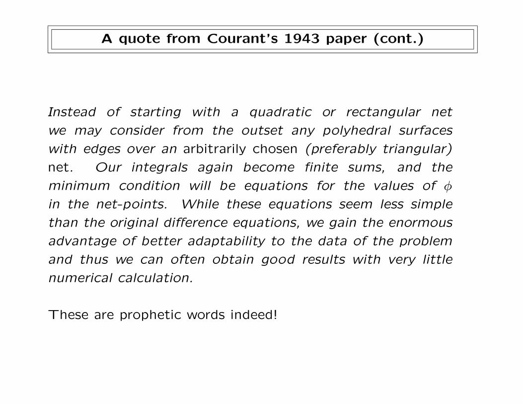
Instead of starting with a quadratic or rectangular net
we may consider from the outset any polyhedral surfaces
with edges over an arbitrarily chosen (preferably triangular)
net. Our integrals again become finite sums, and the
minimum condition will be equations for the values of φ
in the net-points. While these equations seem less simple
than the original difference equations, we gain the enormous
advantage of better adaptability to the data of the problem
and thus we can often obtain good results with very little
numerical calculation.
These are prophetic words indeed!
Key Moments of 20th Century NA (cont.)
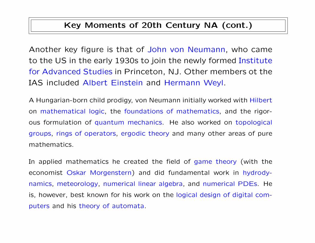
Another key figure is that of John von Neumann, who came
to the US in the early 1930s to join the newly formed Institute
for Advanced Studies in Princeton, NJ. Other members ot the
IAS included Albert Einstein and Hermann Weyl.
A Hungarian-born child prodigy, von Neumann initially worked with Hilbert
on mathematical logic, the foundations of mathematics, and the rigor-
ous formulation of quantum mechanics. He also worked on topological
groups, rings of operators, ergodic theory and many other areas of pure
mathematics.
In applied mathematics he created the field of game theory (with the
economist Oskar Morgenstern) and did fundamental work in hydrody-
namics, meteorology, numerical linear algebra, and numerical PDEs. He
is, however, best known for his work on the logical design of digital com-
puters and his theory of automata.
John von Neumann (1903–1957)
A giant of 20th Century mathematics.
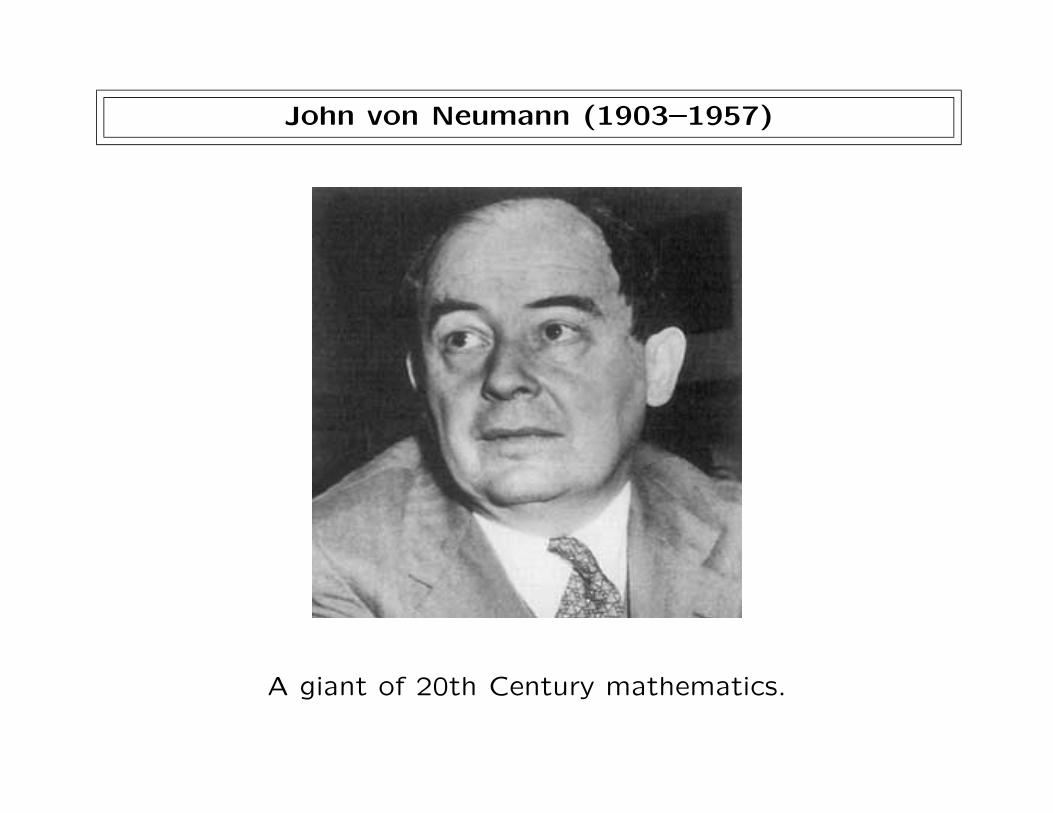
Stan Ulam, Richard Feynman and John von Neumann
(Bandelier, near Los Alamos, NM, late 1940s)
Three key figures in 20th Century science.
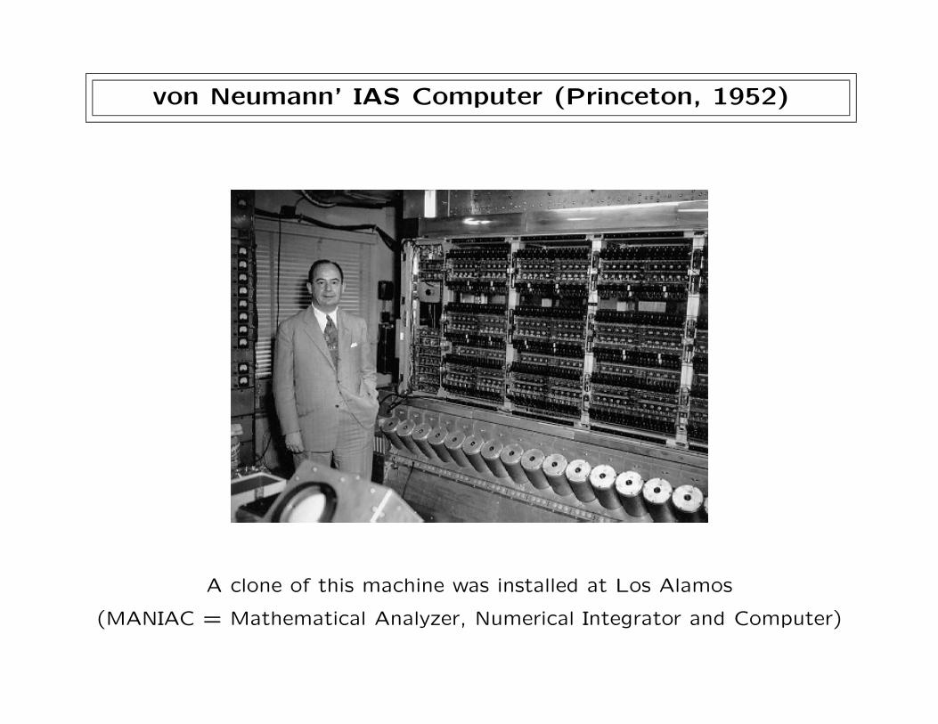
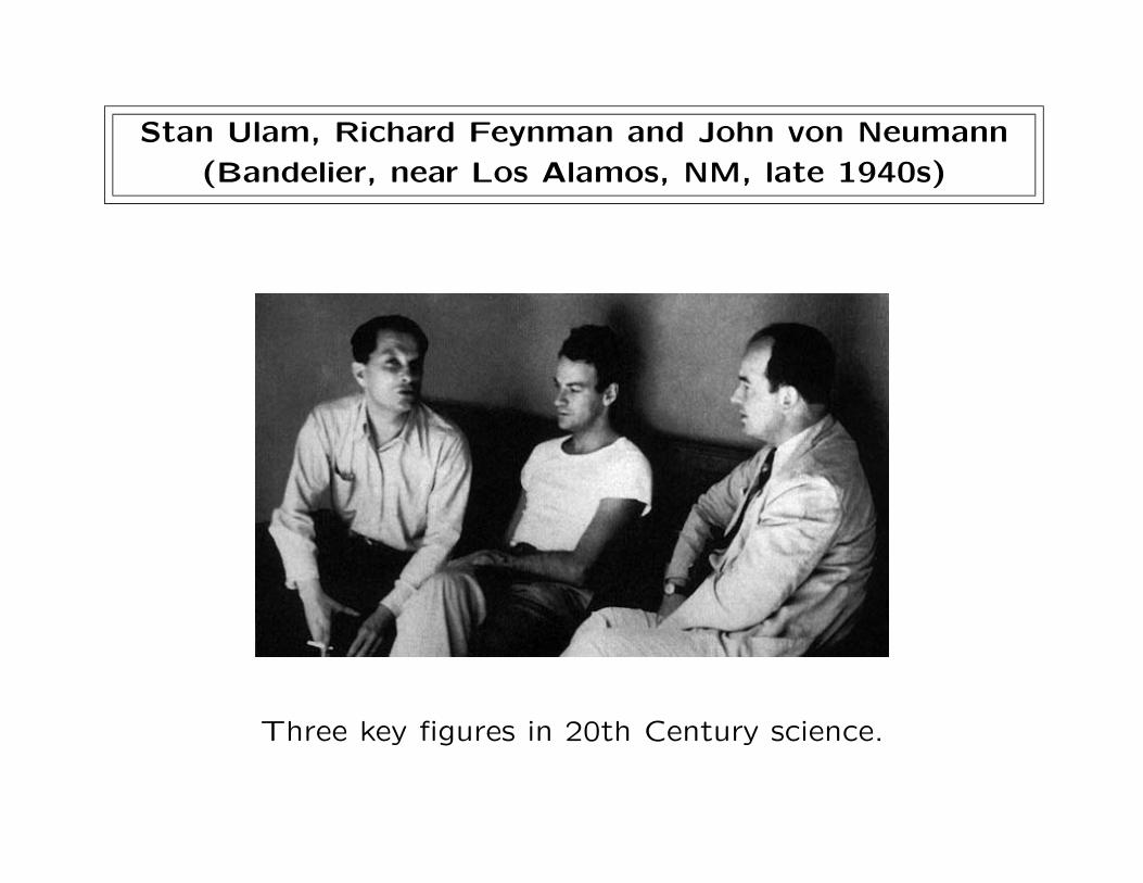
von Neumann’ IAS Computer (Princeton, 1952)
A clone of this machine was installed at Los Alamos
(MANIAC = Mathematical Analyzer, Numerical Integrator and Computer)
Key Moments of 20th Century NA (cont.)
Among von Neumann’s contributions to NA and scientific
computing we mention:
1. The well-known von Neumann stability condition (based
on Fourier analysis) for the time-integration of evolution
problems
2. Pioneering work (mostly with H. Goldstine) in numerical
linear algebra
3. Early contributions to linear programming (later devel-
oped by Dantzig and others)
4. The development (with Metropolis and Ulam) of the
Monte Carlo method
Owing to his enormous prestige as a great mathematician, von Neumann
is often cited as one of the main factors making NA acceptable as a bona
fide mathematical discipline (and not just a collection of recipes).
Key Moments of 20th Century NA (cont.)
J. von Neumann and H. H. Goldstine, Numerical inverting of
matrices of high order, Bull. Amer. Math. Soc., 53 (1947),
pp. 1021–1099.
This long paper is considered by many to mark the beginning
of modern numerical linear algebra. It is mostly devoted to
a detailed round-off error analysis of matrix factorization
and inversion methods. Among other things, it introduces
the notion of condition number κ(A) of an SPD matrix with
respect to inversion. The paper also marks the first use of
backward error analysis, later greatly developed and widely
applied by Wilkinson.
At about the same time (1948), a paper by Alan Turing
provided a similar analysis of Gaussian elimination.
A quote from von Neumann and Goldstine (1947)
From the Preface:
The purpose of this paper is to derive rigorous error esti-
mates in connection with the inverting of matrices of high
order. The reasons for taking up this subject at this time
in such considerable detail are essentially these: First, the
rather widespread revival of mathematical interest in numeri-
cal methods, and the introduction of new procedures and de-
vices which make it both possible and necessary to perform
operations of this type on matrices of much higher orders
than was even remotely practical in the past. Second, the
fact that considerably diverging opinions are now current as
to the extremely high or extremely low precisions which are
required when inverting matrices of order n ≥ 10.
Key Moments of 20th Century NA (cont.)
Numerical linear algebra also received great impetus from
the establishment on the UCLA campus of the Institute for
Numerical Analysis of the National Bureau of Standards
(1947-1954).
Among the main figures associated with INA we mention
George Forsythe, Cornelius Lanczos, Isaac Schoenberg, Olga
Taussky-Todd, John Todd, Magnus Hestenes, and Eduard
Stiefel.
Both the Lanczos algorithm and the Conjugate Gradient
method date to this exciting period. Their widespread use,
however, will have to wait until the 1970s.
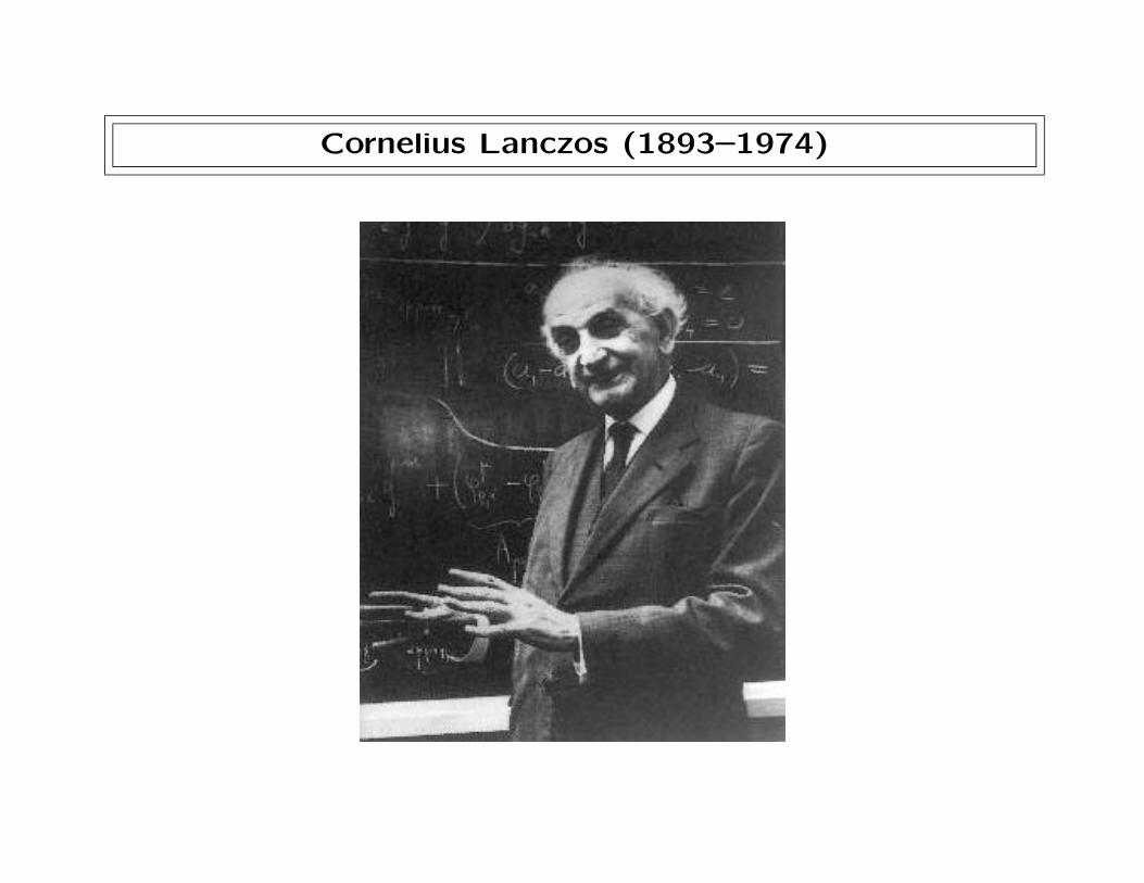
Cornelius Lanczos (1893–1974)

Magnus Hestenes and Eduard Stiefel
Co-discoverers of the Conjugate Gradient Method.
Key Moments of 20th Century NA (cont.)
Other notable figures in numerical linear algebra in the
1950s and 1960s include Wallace Givens (Argonne), Alston
Householder (Oak Ridge), Jim Wilkinson (NPL, UK), Heinz
Rutishauser (ETH Zurich), Alexander Ostrowski (Basel),
John Francis (UK), and Vera Kublanovskaya (USSR); stable
and efficient methods for linear systems and eigenvalue
calculations are due to them.
Important contributions to the area of iterative methods in
this period are due to David Young, Richard Varga, and
Gene Golub.
In the mid-60s, fundamental work by Golub, Velvel Kahan and
others led to stable algorithms for SVD-based least-squares
and pseudoinverse calculations.
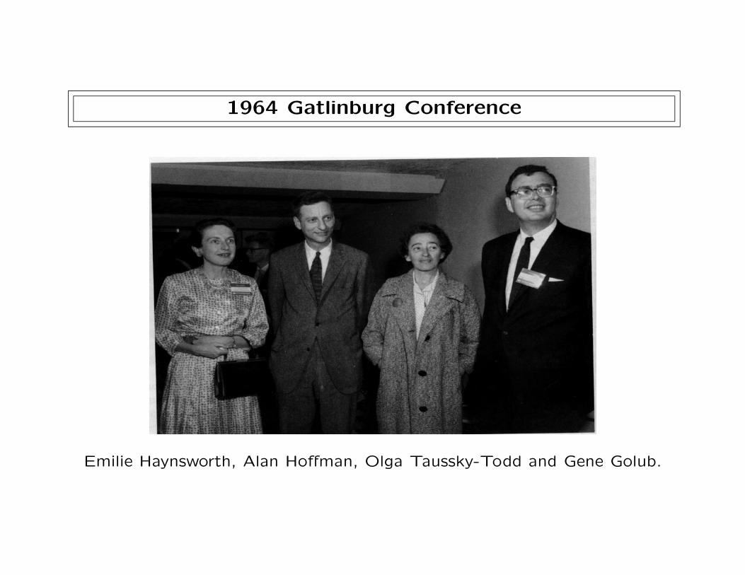
1964 Gatlinburg Conference
Emilie Haynsworth, Alan Hoffman, Olga Taussky-Todd and Gene Golub.
Key Moments of 20th Century NA (cont.)
The 1950s also see great progress in the analysis of
finite difference methods for PDEs (including the famous
equivalence theorem of Peter Lax) and the development
of Alternating Direction Implicit (ADI) and splitting-up
methods by Peaceman, Rachford, Douglas, Birkhoff, Varga,
Young in USA and by Yanenko and others in USSR.
Together with the SOR method, ADI schemes are the method of choice
for the numerical solution of discretized PDEs during much of the 1950s
and 1960s. Only in the 1970s will the Conjugate Gradient method gain
favor, especially after the development of incomplete Cholesky precondi-
tioning. Much credit here goes to John Reid (UK), Koos Meijerink and
Henk van der Vorst (Netherlands), and to a 1976 paper by Gene Golub,
Paul Concus and Dianne O’Leary.
Key Moments of 20th Century NA (cont.)
In the 1960s and 1970s a class of (non-iterative) methods for
solving the Poisson equation on regular grids in near-optimal
time is developed by Buneman, Golub, Buzbee, Nielson
and others. These techniques are closely related to cyclic
reduction and the Fast Fourier Transform (FFT) of Cooley
and Tuckey (1965).
These fast Poisson solvers will later be superseded by
variants of the multigrid method, first studied in USSR by
Fedorenko and Bakhvalov in the 1960s, and later by Achi
Brandt, Wolfgang Hackbusch, and many others.
Chief applications of PDE solvers during this period are in the
areas of nuclear reactor modeling and petroleum engineering.
Key Moments of 20th Century NA (cont.)
The 1980s and 1990s see rapid developments in the field of
Krylov subspace methods for nonsymmetric linear systems
(Young, Saylor, Sonneveld, Eisenstat, Elman, Schulz,
Saad, Freund, Nachtigal, van der Vorst), preconditioning,
multilevel algorithms, and large-scale eigenvalue solvers.
On the theory side, the important Faber-Manteuffel Theo-
rem (1984) settles a question of Golub on the existence of
optimal Krylov methods based on short recurrences.
We also mention the impact of parallel computing, stimulat-
ing the development of domain decomposition schemes by
Lions, Widlund, and many others.
Additional references and resources
G. Birkhoff, Solving Elliptic Problems: 1930–1980, in M. H. Schulz, Ed.,Elliptic Problem Solvers, Academic Press, NY, 1981.
C. Brezinski and L. Wuytack, Eds., Numerical Analysis: HistoricalDevelopments in the Twentieth Century, North-Holland, Amsterdam,2001.
M. R. Hestenes and J. Todd, Mathematicians Learning to Use Comput-ers. The Institute for Numerical Analysis, UCLA, 1947–1954. NationalInstitute of Standards and Technology and Mathematical Association ofAmerica, Washington, DC, 1991.
S. G. Nash, Ed., A History of Scientific Computing, ACM Press andAddison-Wesley Publishing Co., NY, 1990.
The SIAM History Project at http://history.siam.org contains a numberof articles and transcripts of interviews—highly recommended!
PART II
The early history of matrix iterations
Iterative methods prior to about 1930
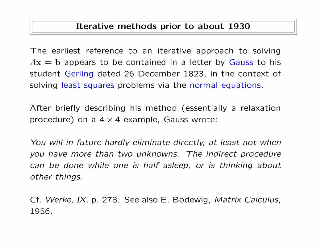
The earliest reference to an iterative approach to solving
Ax = b appears to be contained in a letter by Gauss to his
student Gerling dated 26 December 1823, in the context of
solving least squares problems via the normal equations.
After briefly describing his method (essentially a relaxation
procedure) on a 4× 4 example, Gauss wrote:
You will in future hardly eliminate directly, at least not when
you have more than two unknowns. The indirect procedure
can be done while one is half asleep, or is thinking about
other things.
Cf. Werke, IX, p. 278. See also E. Bodewig, Matrix Calculus,
1956.
Iterative methods prior to about 1930 (cont.)
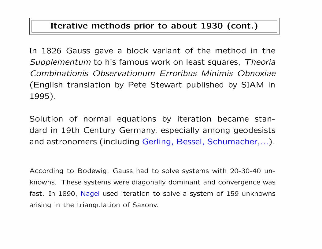
In 1826 Gauss gave a block variant of the method in the
Supplementum to his famous work on least squares, Theoria
Combinationis Observationum Erroribus Minimis Obnoxiae
(English translation by Pete Stewart published by SIAM in
1995).
Solution of normal equations by iteration became stan-
dard in 19th Century Germany, especially among geodesists
and astronomers (including Gerling, Bessel, Schumacher,...).
According to Bodewig, Gauss had to solve systems with 20-30-40 un-
knowns. These systems were diagonally dominant and convergence was
fast. In 1890, Nagel used iteration to solve a system of 159 unknowns
arising in the triangulation of Saxony.
Iterative methods prior to about 1930 (cont.)
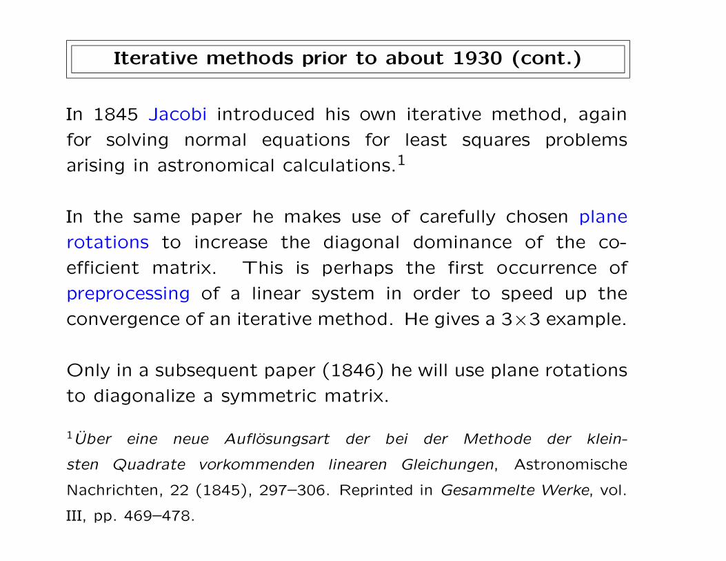
In 1845 Jacobi introduced his own iterative method, again
for solving normal equations for least squares problems
arising in astronomical calculations.1
In the same paper he makes use of carefully chosen plane
rotations to increase the diagonal dominance of the co-
efficient matrix. This is perhaps the first occurrence of
preprocessing of a linear system in order to speed up the
convergence of an iterative method. He gives a 3×3 example.
Only in a subsequent paper (1846) he will use plane rotations
to diagonalize a symmetric matrix.
1Uber eine neue Auflosungsart der bei der Methode der klein-
sten Quadrate vorkommenden linearen Gleichungen, Astronomische
Nachrichten, 22 (1845), 297–306. Reprinted in Gesammelte Werke, vol.
III, pp. 469–478.
Jacobi’s example
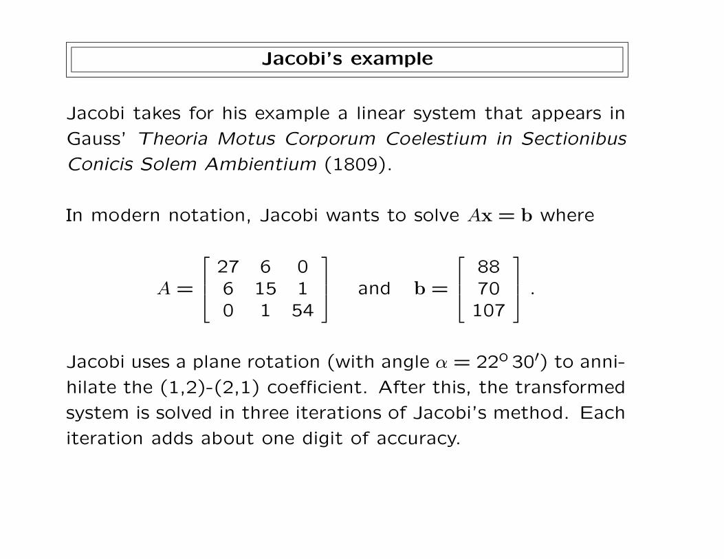
Jacobi takes for his example a linear system that appears in
Gauss’ Theoria Motus Corporum Coelestium in Sectionibus
Conicis Solem Ambientium (1809).
In modern notation, Jacobi wants to solve Ax = b where
A =
27 6 06 15 10 1 54
and b =
8870
107
.Jacobi uses a plane rotation (with angle α = 22o 30′) to anni-
hilate the (1,2)-(2,1) coefficient. After this, the transformed
system is solved in three iterations of Jacobi’s method. Each
iteration adds about one digit of accuracy.
Iterative methods prior to about 1930 (cont.)
Again in the context of least squares, in 1874 another
German, Seidel, publishes his own iterative method.
The paper contains what we now (inappropriately) call
the Gauss–Seidel method, which he describes as an
improvement over Jacobi’s method.
Seidel notes that the unknowns do not have to be pro-
cessed cyclically (in fact, he advises against it!); instead,
one could choose to update at each step the unknown
with the largest residual. He seems to be unaware that
this is precisely Gauss’ method.
In the same paper, Seidel mentions a block variant of his scheme. He
also notes that the calculations can be computed to variable accuracy,
using fewer decimals in the first iterations. His linear systems had up
to 72 unknowns.
Iterative methods prior to about 1930 (cont.)
Another important 19th Century development that is
worth mentioning were the independent proofs of con-
vergence by Nekrasov (1885) and by Pizzetti (1887) of
Seidel’s method for systems of normal equations (more
generally, SPD systems).
These authors were the first to note that a necessary and
sufficient condition for the convergence of the method
(for an arbitrary initial guess x0) is that all the eigenvalues
of the iteration matrix must satisfy |λ| < 1. Nekrasov
and Mehmke (1892) also gave examples to show that
convergence can be slow.
Nekrasov seems to have been the first to relate the rate of convergence
to the dominant eigenvalue of the iteration matrix. The treatment is
still in terms of determinants, and no use is made of matrix notation.
Iterative methods prior to about 1930 (cont.)
In the early 20th century we note the following important
contributions:
• The method of Richardson (1910);
• The method of Liebmann (1918).
These papers mark the first use of iterative methods in
the solution of finite difference approximations to elliptic
PDEs.
Richardson’s method is still well known today, and can be
regarded as an acceleration of Jacobi’s method by means
of over- or under-relaxation factors. Liebmann’s method
is identical with Seidel’s.
Iterative methods prior to about 1930 (cont.)
The first systematic treatment of iterative methods
for solving linear systems appeared in a paper by the
famed applied mathematician Richard von Mises and his
collaborator (and later wife) Hilda Pollaczek-Geiringer,
titled Praktische Verfharen der Gleichungsauflosung
(ZAMM 9, 1929, pp. 58–77).
This was a rather influential paper. In it, the authors
gave conditions for the convergence of Jacobi’s and
Seidel’s methods, the notion of diagonal dominance
playing a central role.
The paper also studied a stationary version of Richard-
son’s method, which will be later called Mises’ method
by later authors.
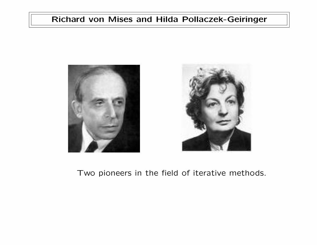
Richard von Mises and Hilda Pollaczek-Geiringer
Two pioneers in the field of iterative methods.
Mauro Picone and the INAC
The paper by von Mises and Pollaczek-Geiringer was
read and appreciated by Mauro Picone (1885-1977)
and his collaborators at the Istituto Nazionale per le
Applicazioni del Calcolo (INAC).
The INAC was among the first institutions in the
world entirely devoted to the development of numerical
analysis. Both basic research and applications were
pursued by the INAC staff.
The Institute had been founded in 1927 by Picone, who was at that
time professor of Infinitesimal Analysis at the University of Naples.
In 1932 Picone moved to the University of Rome, and the INAC was
transferred there. It became a CNR institute in 1933.
Mauro Picone and the INAC (cont.)
Picone’s interest in numerical computing dated back to
his service as an artillery officer in WWI, when he was
put to work on ballistic tables.
The creation of the INAC required great perseverance
and political skill on his part, since most of the mathe-
matical establishment of the time was either indifferent
or openly against it.
Picone’s own training was in classical (“hard”) analysis. He worked
mostly on the theory of differential equations and in the calculus of
variations. He was also keenly interested in constructive and compu-
tational functional-analytic methods.
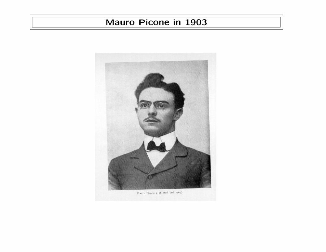
Mauro Picone in 1903
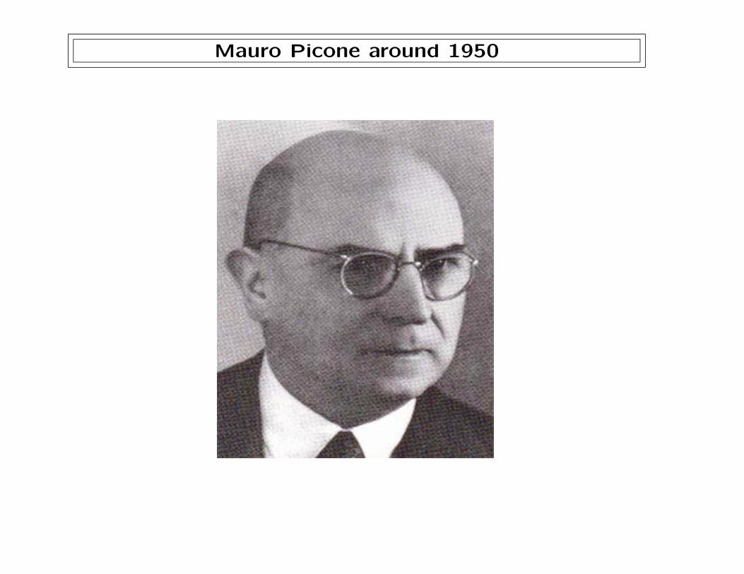
Mauro Picone around 1950
Mauro Picone and the INAC (cont.)
Throughout the 1930’s and beyond, under Picone’s
direction, the INAC employed a number of young math-
ematicians, many of whom later became very well known.
INAC researchers did basic research and also worked on
a large number of applied problems supplied by industry,
government agencies, and the Italian military. Picone was
fond of saying that
Matematica Applicata = Matematica Fascista
In the 1930s the INAC also employed up to eleven computers and
draftsmen. These were highly skilled men and women who were
responsible for carrying out all the necessary calculations using a
variety of mechanical, electro-mechanical, and graphical devices.
Mauro Picone and the INAC (cont.)
As early as 1932, Picone designed and taught one of
the first courses on numerical methods ever offered
at an Italian university (the course was called Calcoli
Numerici e Grafici). The course was taught in the
School of Statistical and Actuarial Sciences, because
Picone’s colleagues in the Mathematics Institute denied
his request to have the course listed among the electives
for the degree in Mathematics.
The course covered root finding, maxima and minima,
solutions of linear and nonlinear systems, interpolation,
numerical quadrature, and practical Fourier analysis.
Both Jacobi’s and Seidel’s method are discussed (including block
variants). Picone’s course was not very different from current
introductory classes in numerical analysis.
Mauro Picone and the INAC (cont.)
In the chapter on linear systems, Picone wrote:
The problem of solving linear systems has enormous importance in
applied mathematics, since nearly all computational procedures lead
to such problem. The problem can be considered as a multivariate
generalization of ordinary division... While for ordinary division there
exist automatic machines, things are not so for the solution of
linear systems, although some great minds have set themselves this
problem in the past. Indeed, the first researches go back to Lord
Kelvin. Recently, Professor Mallock of Cambridge University has
built a highly original electrical machine which can solve systems of
n ≤ 10 equations in as many unknowns. This and other recent ef-
forts, however, are far from giving a practical solution to the problem.
Lamberto Cesari’s work on iterative methods
Lamberto Cesari (Bologna, 1910; Ann Arbor, MI, 1990)
studied at the Scuola Normale in Pisa under L. Tonelli,
then in 1934 went to Germany to specialize under the
famous mathematician C. Caratheodory. After his return
from Germany, Cesari joined the INAC in Rome.
While at INAC Cesari wrote the paper Sulla risoluzione dei
sistemi di equazioni lineari per approssimazioni successive
(La Ricerca Scientifica, 8, 1937, pp. 512–522.)
Cesari later became a leading expert in various branches of mathemat-
ical analysis and optimization. In 1948 he emigrated to the US, where
he had a brilliant career, first at Purdue, then at Michigan.

Lamberto Cesari (1910-1990)
Lamberto Cesari’s 1937 paper
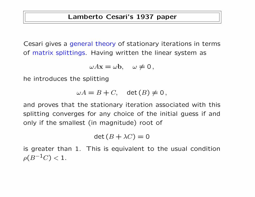
Cesari gives a general theory of stationary iterations in terms
of matrix splittings. Having written the linear system as
ωAx = ωb, ω 6= 0 ,
he introduces the splitting
ωA = B + C, det (B) 6= 0 ,
and proves that the stationary iteration associated with this
splitting converges for any choice of the initial guess if and
only if the smallest (in magnitude) root of
det (B + λC) = 0
is greater than 1. This is equivalent to the usual condition
ρ(B−1C) < 1.
Lamberto Cesari’s 1937 paper (cont.)
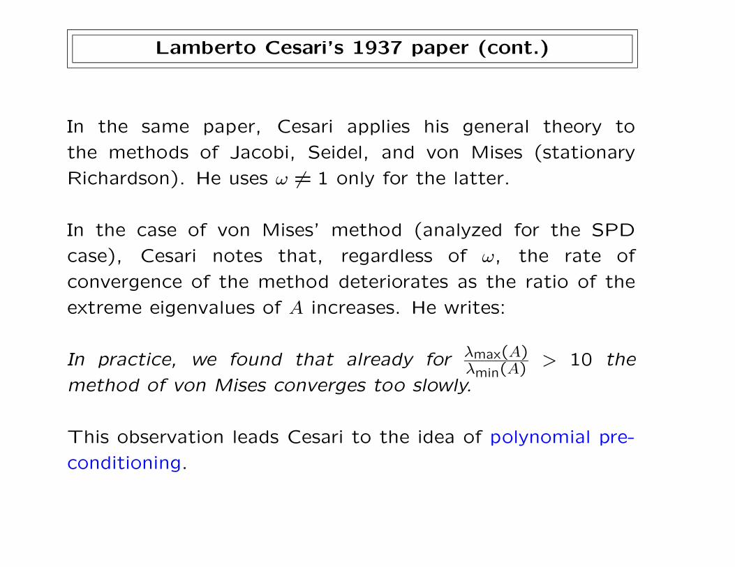
In the same paper, Cesari applies his general theory to
the methods of Jacobi, Seidel, and von Mises (stationary
Richardson). He uses ω 6= 1 only for the latter.
In the case of von Mises’ method (analyzed for the SPD
case), Cesari notes that, regardless of ω, the rate of
convergence of the method deteriorates as the ratio of the
extreme eigenvalues of A increases. He writes:
In practice, we found that already for λmax(A)λmin(A) > 10 the
method of von Mises converges too slowly.
This observation leads Cesari to the idea of polynomial pre-
conditioning.
Lamberto Cesari’s 1937 paper (cont.)
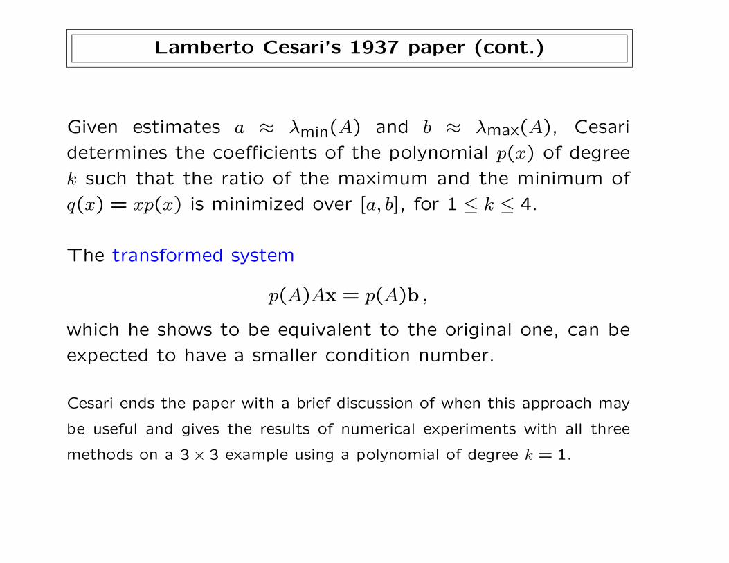
Given estimates a ≈ λmin(A) and b ≈ λmax(A), Cesari
determines the coefficients of the polynomial p(x) of degree
k such that the ratio of the maximum and the minimum of
q(x) = xp(x) is minimized over [a, b], for 1 ≤ k ≤ 4.
The transformed system
p(A)Ax = p(A)b ,
which he shows to be equivalent to the original one, can be
expected to have a smaller condition number.
Cesari ends the paper with a brief discussion of when this approach may
be useful and gives the results of numerical experiments with all three
methods on a 3× 3 example using a polynomial of degree k = 1.
Lamberto Cesari’s 1937 paper (cont.)
Cesari’s paper was not without influence: it is cited,
sometimes at length, in important papers by Forsythe
(1952-1953) and in the books by Bodewig (1956), Faddeev
& Faddeeva (1960), Householder (1964), Wachspress
(1966) and Saad (2003) among others.
It is, however, not cited in the influential books of Varga
(1962) and Young (1971).
Cesari’s paper is important for our story also because of the
effect it had on a former student and assistant of Picone.
Cimmino’s method
Gianfranco Cimmino (Naples, 1908; Bologna, 1989) grad-
uated at Naples with Picone in 1927 with a thesis on
approximate solution methods for the heat equation in 2D.
After a period spent at INAC and a study stay in Germany
(again with Caratheodory), he undertook a brilliant academic
career. He became a full professor in 1938, and in 1939
moved to the chair of Mathematical Analysis at Bologna,
where he spent his entire career.
Cimmino’s work was mostly in analysis: theory of linear elliptic PDEs,
calculus of variations, integral equations, functional analysis, etc. He also
wrote 5-6 short papers on matrix computations.
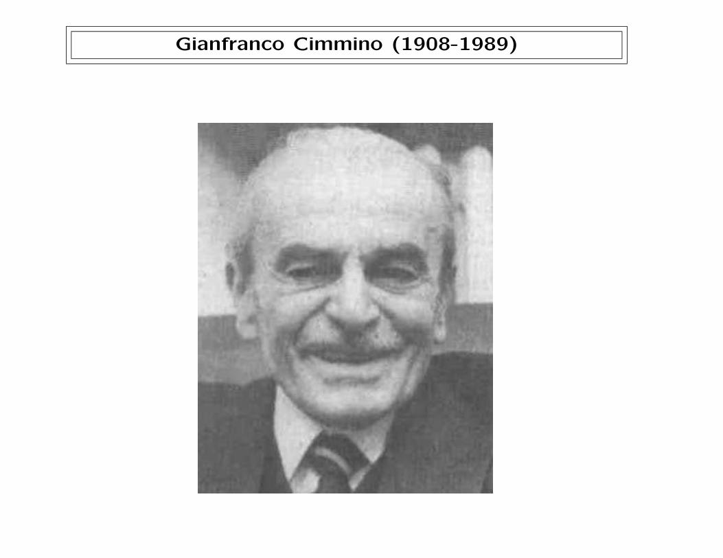
Gianfranco Cimmino (1908-1989)
Cimmino’s method (cont.)
In 1938 La Ricerca Scientifica published a short (8 pages)
paper by Cimmino, titled Calcolo approssimato per le
soluzioni dei sistemi lineari.
As Picone himself explained in a brief introductory note,
after reading Cesari’s paper Cimmino reminded him of a
method that he had developed around 1932 while he was
at INAC. Cimmino’s method did not appear to fit under
Cesari’s “systematic treatment,” yet
it is most worthy of consideration in the applications because of its gen-
erality, its efficiency and, finally, because of its guaranteed convergence
which can make the method practicable in many cases. Therefore, I
consider it useful to publish in this journal Prof. Cimmino’s note on the
above mentioned method, note that he has accepted to write upon my
insistent invitation.
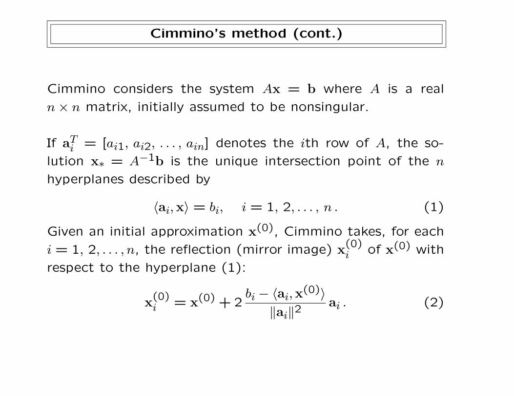
Cimmino’s method (cont.)
Cimmino considers the system Ax = b where A is a real
n× n matrix, initially assumed to be nonsingular.
If aTi = [ai1, ai2, . . . , ain] denotes the ith row of A, the so-
lution x∗ = A−1b is the unique intersection point of the n
hyperplanes described by
〈ai,x〉 = bi, i = 1, 2, . . . , n . (1)
Given an initial approximation x(0), Cimmino takes, for each
i = 1, 2, . . . , n, the reflection (mirror image) x(0)i of x(0) with
respect to the hyperplane (1):
x(0)i = x(0) + 2
bi − 〈ai,x(0)〉‖ai‖2
ai . (2)
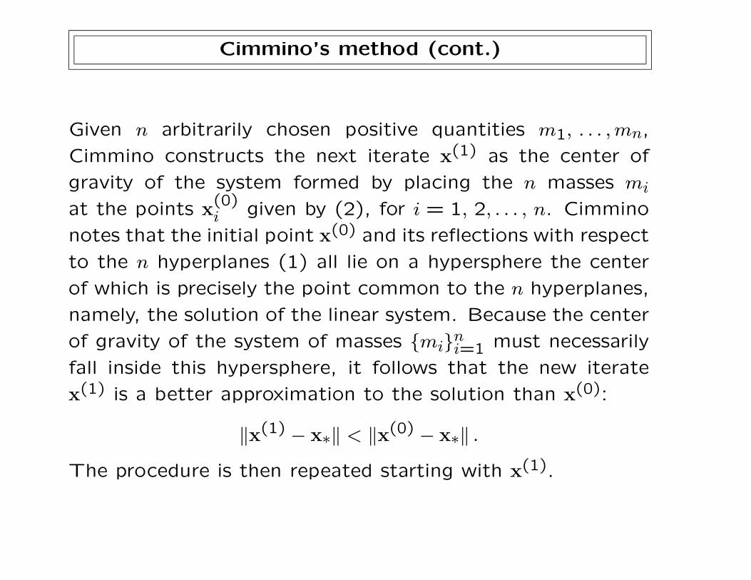
Cimmino’s method (cont.)
Given n arbitrarily chosen positive quantities m1, . . . ,mn,
Cimmino constructs the next iterate x(1) as the center of
gravity of the system formed by placing the n masses mi
at the points x(0)i given by (2), for i = 1, 2, . . . , n. Cimmino
notes that the initial point x(0) and its reflections with respect
to the n hyperplanes (1) all lie on a hypersphere the center
of which is precisely the point common to the n hyperplanes,
namely, the solution of the linear system. Because the center
of gravity of the system of masses {mi}ni=1 must necessarily
fall inside this hypersphere, it follows that the new iterate
x(1) is a better approximation to the solution than x(0):
‖x(1) − x∗‖ < ‖x(0) − x∗‖ .
The procedure is then repeated starting with x(1).
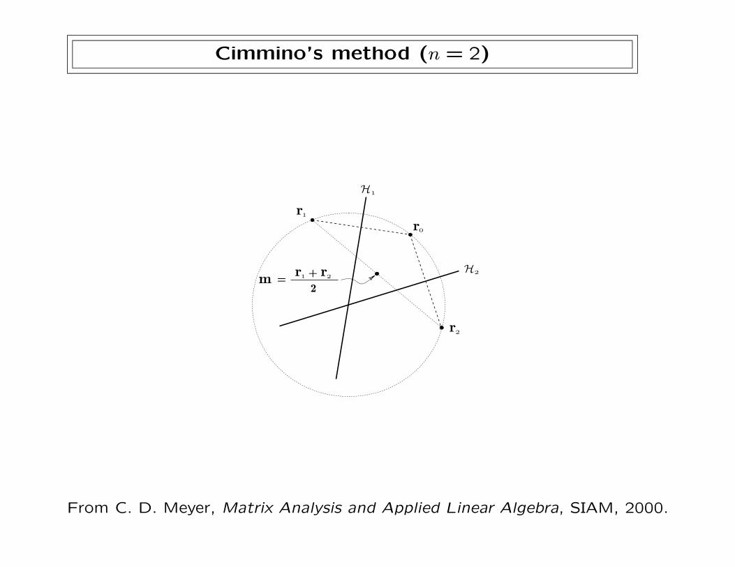
Cimmino’s method (n = 2)
From C. D. Meyer, Matrix Analysis and Applied Linear Algebra, SIAM, 2000.
Cimmino’s method (cont.)
Cimmino proves that his method is always convergent.
In the same paper Cimmino shows that the iterates converge
to a solution of Ax = b even in the case of a singular (but
consistent) system, provided that rank (A) ≥ 2.
He then notes that the sequence {x(k)} converges even
when the linear system is inconsistent, always provided that
rank (A) ≥ 2. Much later (1967) Cimmino wrote:
The latter observation, however, is just a curiosity, being
obviously devoid of any practical usefulness. [sic!]
It can be shown that for an appropriate choice of the masses
mi, the sequence {x(k)} converges to the minimum 2-norm
solution of ‖b−Ax‖2 = min.
Cimmino’s method (cont.)
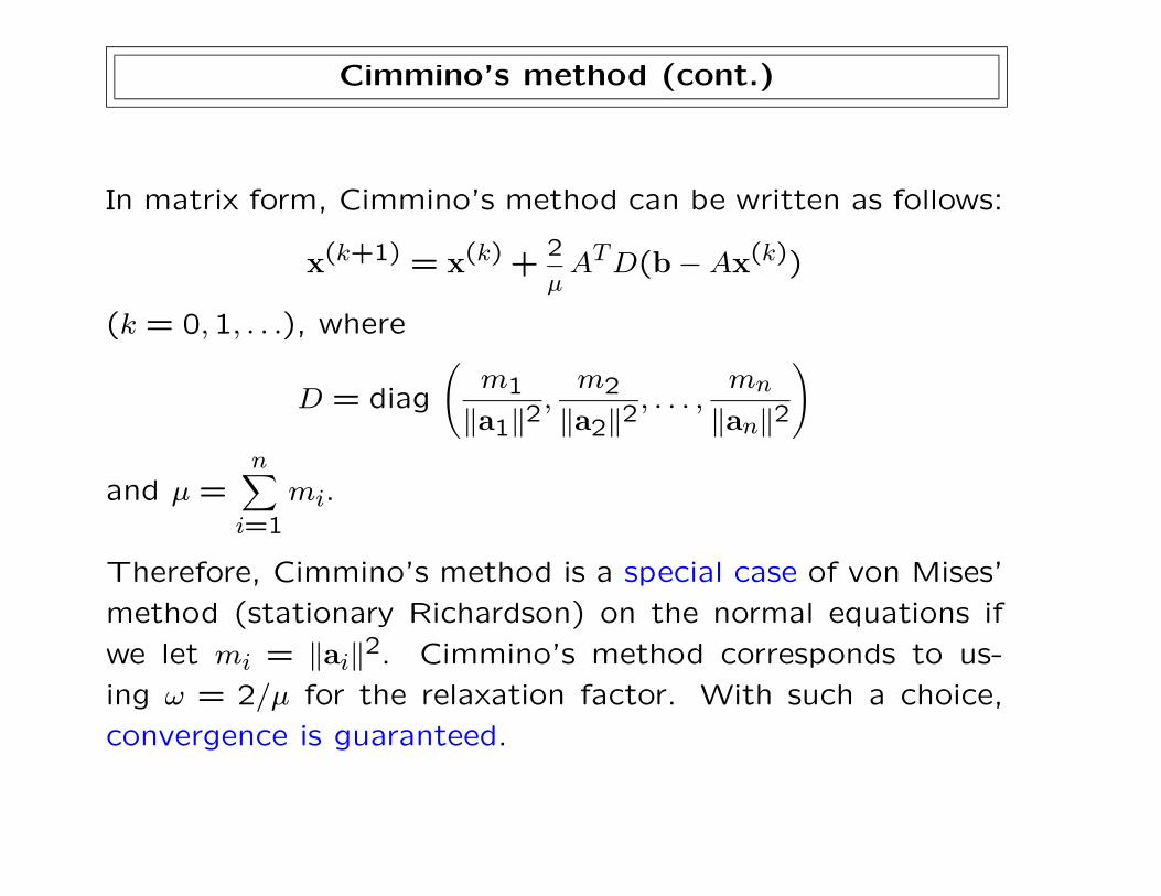
In matrix form, Cimmino’s method can be written as follows:
x(k+1) = x(k) +2
µATD(b−Ax(k))
(k = 0,1, . . .), where
D = diag
(m1
‖a1‖2,m2
‖a2‖2, . . . ,
mn
‖an‖2
)
and µ =n∑i=1
mi.
Therefore, Cimmino’s method is a special case of von Mises’
method (stationary Richardson) on the normal equations if
we let mi = ‖ai‖2. Cimmino’s method corresponds to us-
ing ω = 2/µ for the relaxation factor. With such a choice,
convergence is guaranteed.
Cimmino’s legacy
Cimmino’s method, like the contemporary (and related)
method of Kaczmarz, did not attract much attention until
many years later.
Although it was described by Forsythe (1953) and in the
books of Bodewig (1956), Householder (1964), Gastinel
(1966) and others, I was able to find only 8 journal citations
of Cimmino’s 1938 paper until 1980.
After 1980, the number of papers and books citing Cimmino’s
(as well as Kaczmarz’s) method picks up dramatically, and it
is now in the hundreds. Moreover, both methods have been
reinvented several times.
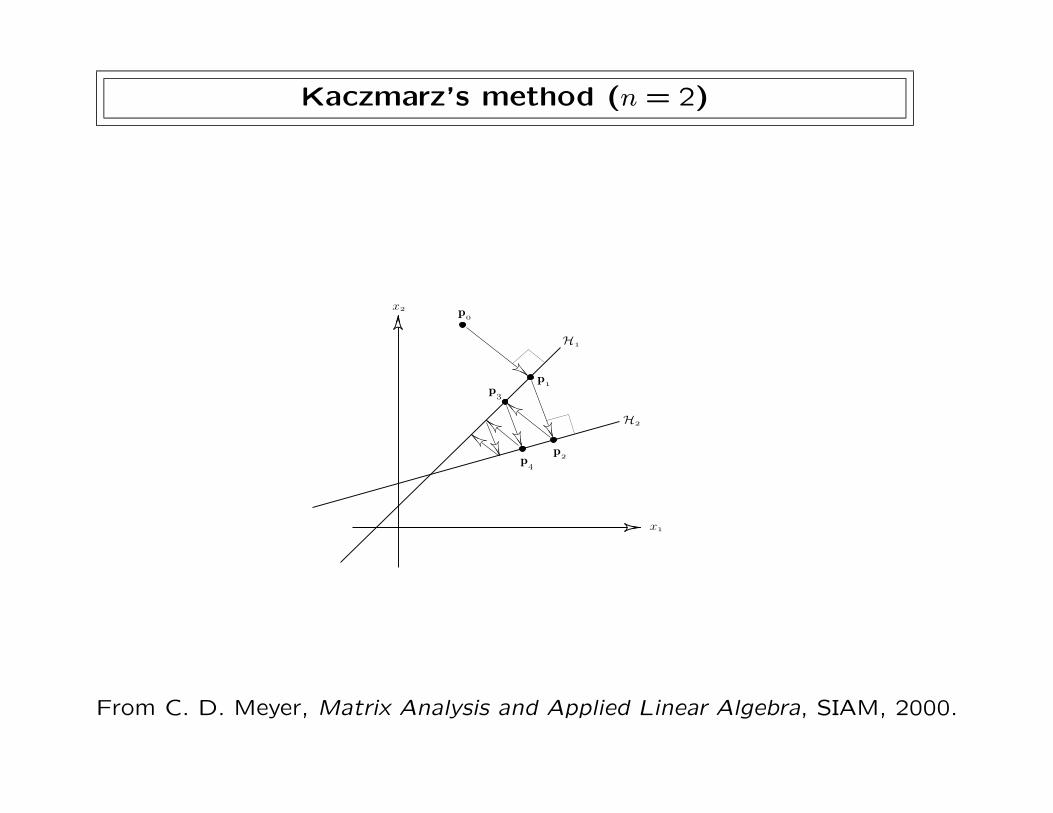
Kaczmarz’s method (n = 2)
From C. D. Meyer, Matrix Analysis and Applied Linear Algebra, SIAM, 2000.
Cimmino’s legacy (cont.)
Two major reasons for this surge in popularity are the
fact that the method has the regularizing property when
applied to discrete ill-posed problems, and the high degree
of parallelism of the algorithm.
Today, Cimmino’s method is rarely used to solve linear
systems. Rather, it forms the basis for algorithms that are
used to solve systems of inequalities (the so-called convex
feasibility problem), and it has applications in computerized
tomography, radiation treatment planning, medical imaging,
etc.
Indeed, most citations occur in the medical physics literature,
an outcome that would have pleased Gianfranco Cimmino.
References
M. Benzi, Gianfranco Cimmino’s contribution to numerical
mathematics, Atti del Seminario di Analisi Matematica
dell’Universita di Bologna, Technoprint, 2005, pp. 87–109.
Y. Saad and H. A. van der Vorst, Iterative solution of linear
systems in the 20th Century, J. Comput. Applied. Math., 123
(2000), pp. 1–33.


![3. Numerical integration (Numerical quadrature). Given the continuous function f(x) on [a,b], approximate Newton-Cotes Formulas: For the given abscissas,](https://img.pdfslide.us/doc/110x75/56649e175503460f94b02909/3-numerical-integration-numerical-quadrature-given-the-continuous-function.jpg)


![CHAPTER 12 Numerical Integration · In general, we can derive numerical integration methods by splitting the interval [ a , b ] into small subintervals, approximate f by a polynomial](https://img.pdfslide.us/doc/110x75/6102b77fa4e40412a1036ea2/chapter-12-numerical-integration-in-general-we-can-derive-numerical-integration.jpg)