Embed Size (px)
Citation preview

Key Features and Terminology

CSiBridge®
Key Features and Terminology
BRG102816M3 Rev. 0 Proudly developed in the United States of America October 2016

Copyright
Copyright Computers & Structures, Inc., 1978-2016 All rights reserved. The CSI Logo® and CSiBridge® are registered trademarks of Computers & Structures, Inc. Watch & LearnTM is a trademark of Computers & Structures, Inc. Adobe and Acrobat are registered trademarks of Adobe Systems Incorported. AutoCAD is a registered trademark of Autodesk, Inc. The computer program CSiBridge® and all associated documentation are proprietary and copyrighted products. Worldwide rights of ownership rest with Computers & Structures, Inc. Unlicensed use of this program or reproduction of documentation in any form, without prior written authorization from Computers & Structures, Inc., is explicitly prohibited.
No part of this publication may be reproduced or distributed in any form or by any means, or stored in a database or retrieval system, without the prior explicit written permission of the publisher.
Further information and copies of this documentation may be obtained from:
Computers & Structures, Inc. www.csiamerica.com [email protected] (for general information) [email protected] (for technical support)

DISCLAIMER
CONSIDERABLE TIME, EFFORT AND EXPENSE HAVE GONE INTO THE DEVELOPMENT AND TESTING OF THIS SOFTWARE. HOWEVER, THE USER ACCEPTS AND UNDERSTANDS THAT NO WARRANTY IS EXPRESSED OR IMPLIED BY THE DEVELOPERS OR THE DISTRIBUTORS ON THE ACCURACY OR THE RELIABILITY OF THIS PRODUCT.
THIS PRODUCT IS A PRACTICAL AND POWERFUL TOOL FOR STRUCTURAL DESIGN. HOWEVER, THE USER MUST EXPLICITLY UNDERSTAND THE BASIC ASSUMPTIONS OF THE SOFTWARE MODELING, ANALYSIS, AND DESIGN ALGORITHMS AND COMPENSATE FOR THE ASPECTS THAT ARE NOT ADDRESSED.
THE INFORMATION PRODUCED BY THE SOFTWARE MUST BE CHECKED BY A QUALIFIED AND EXPERIENCED ENGINEER. THE ENGINEER MUST INDEPENDENTLY VERIFY THE RESULTS AND TAKE PROFESSIONAL RESPONSIBILITY FOR THE INFORMATION THAT IS USED.
Contents
1 Welcome to CSiBridge
1.1 Introduction 1-1
1.2 History and Advantages of CSiBridge 1-3
1.3 What CSiBridge Can Do! 1-4
1.4 An Integrated Approach 1-5
1.5 Modeling Features 1-5
1.6 Analysis Features 1-7
1.7 Design Features 1-8
1.8 Seismic Features 1-8
1.9 Rating Features 1-9
i
CSiBridge – Key Features and Terminology
1.10 Advanced Features 1-9
1.11 An Intuitive Process 1-10
1.12 Work Flow 1-11
2 Getting Started
2.1 Installing CSiBridge 2-1
2.2 If You are Upgrading 2-1
2.3 About the Manuals 2-2
2.4 “Watch & Learn” Movies 2-3
2.5 CSI Knowledge Base 2-3
2.6 Technical Support 2-4
2.7 Help Us to Help You 2-4
3 Lanes
3.1 Centerline and Direction 3-1
3.2 Eccentricity 3-2
3.3 Width 3-2
3.4 Interior and Exterior Edges 3-2
3.5 Discretization 3-3
ii

Contents
4 Influence Lines and Surfaces
4.1 Overview 4-1
4.2 Influence Line and Surfaces 4-2
5 Vehicle Live Loads
5.1 Direction of Loading 5-1
5.2 Distribution of Loads 5-1
5.3 Axle Loads 5-2
5.4 Uniform Loads 5-2
5.5 Minimum Edge Distances 5-2
5.6 Restricting a Vehicle to the Lane Length 5-3
5.7 Application of Loads to the Influence Surface 5-3
5.7.1 Option to Allow Reduced Response Severity 5-4 5.7.2 Width Effects 5-4
5.8 Length Effects 5-4
5.8.1 Concentrated (Axle) Loads 5-5 5.8.2 Distributed Loads 5-5
5.9 Application of Loads in Multi-Step Analysis 5-6
6 General Vehicle
6.1 Specification 6-2
6.2 Moving the Vehicle 6-3
iii
CSiBridge – Key Features and Terminology
7 Vehicle Response Components
7.1 Superstructure (Span) Moment 7-1
7.2 Negative Superstructure (Span) Moment 7-2
7.3 Reactions at Interior Supports 7-3
8 Standard Vehicles
8.1 Hn-44 and HSn-44 8-1
8.2 Hn-44L and HSn-44L 8-2
8.3 AML 8-2
8.4 HL-93k, HL-93M, and HL-93S 8-2
8.5 P5, P7, P9, P11, and P13 8-3
8.6 Cooper E 80 8-3
8.7 UICn 8-3
8.8 RL 8-3
9 Vehicle Classes
9.1 Vehicle Class Definitions 9-1
10 Moving Load Load Cases
10.1 AASHTO HS Loading 10-2
10.2 AASHTO HL Loading 10-4
iv
Contents
10.3 Caltrans Permit Loading 10-5
10.4 Restricted Caltrans Permit Loading 10-7
11 Moving Load Response Control
11.1 Bridge Response Groups 11-1
11.2 Correspondence 11-2
11.3 Influence Line Tolerance 11-2
11.4 Exact and Quick Response calculation 11-3
12 Step-By-Step Analysis
12.1 Loading 12-2
12.2 Static Analysis 12-2
12.3 Time-History Analysis 12-3
12.4 Enveloping and Load Combinations 12-3
12.5 Computational Considerations 12-4
v
Chapter 1 Welcome to CSiBridge
CSiBridge has been created as the ultimate, easy-to-use, integrated soft-ware program for modeling, analysis, and design of bridge structures. The ease with which all of these critical tasks can be accomplished makes CSiBridge the most versatile and productive bridge design pack-age in the industry. Welcome to the new world of CSiBridge!
1.1 Introduction
A CSiBridge model may be analyzed to determine the response of bridge structures to the weight of vehicle live loads. Considerable power and flexibility is provided for determining the maximum and minimum dis-placements, forces, and stresses from multiple-lane loads on complex structures, such as highway interchanges. The effects of vehicle live loads can be combined with static and dynamic loads, and envelopes of the response can be computed.
The bridge to be analyzed can be created using templates accessed through the File > New command; built manually using frame, shell, sol-id, and link elements defined using the Bridge Wizard on the Home tab or the individual commands on the Components tab; or by combining these features. The superstructure can be represented by a simple “spine”
Introduction 1 - 1
CSiBridge – Key Features and Terminology
(or “spline”) model using frame elements, or it can be modeled in full 3-dimensional detail using shell or solid elements.
Lanes are defined that represent where the live loads can act on the su-perstructure. Lanes may have width and can follow any straight or curved path. Multiple lanes need not be parallel or of the same length so that complex traffic patterns may be considered. The program automati-cally determines how the lanes load the superstructure, even if they are eccentric to a spine model. Conventional influence lines and surfaces for loading of each lane can be displayed for any response quantity.
Vehicle live loads can be selected from a set of standard highway and railway vehicles, or users can specify their own vehicle live loads. Vehi-cles are grouped in vehicle classes, such that the most severe loading of each class governs.
Two types of live-load analysis can be considered:
Influence-based enveloping analysis: Vehicles move in both di-rections along each lane of the bridge. Using the influence sur-face, vehicles are automatically located at such positions along the length and width of the lanes to produce the maximum and mini-mum response quantities throughout the structure. Each vehicle may be allowed to act on every lane or be restricted to certain lanes. The program can automatically find the maximum and min-imum response quantities throughout the structure for placement of different vehicles in different lanes. For each maximum or min-imum extreme response quantity, the corresponding values for the other components of response can also be computed.
Step-by-step analysis: Any number of vehicles can be run simul-taneously on the lanes, each with its own starting time, position, direction and speed. Step-by-step static or time-history analysis can be performed, with nonlinear effects included if desired.
For most design purposes the envelope-type analysis using moving-load load cases is most appropriate. For special studies and unusual permit vehicles, the step-by-step approach can be valuable.
1 - 2 Introduction
Chapter 1 Welcome to CSiBridge
1.2 History and Advantages of CSiBridge
Bridges are a very special class of structures. They are characterized by their complexity in geometry and loading. The geometry of a bridge structure is defined by a number of features that include the alignment (both vertical and horizontal) and the superstructure type. The geometry of a bridge may become more complex when certain features of the bridge vary across spans such as girder depths, deck widths and girder properties. Support conditions can also contribute to the complexity of a bridge model.
Recognition of the unique characteristics of the bridge structure led to the development of CSiBridge more than ten years ago. Originally a bridge module was added to SAP2000, which gave users the ability to generate simple and complex bridge models using all of the powerful features within SAP2000. Now, the analysis, design and rating of simple to complex bridges may be handled using a single program: CSiBridge. The all new CSiBridge incorporates a ribbon-based interface that pro-vides for an easy-to-use and intuitive workflow.
CSiBridge’s parametrically defined bridge models greatly reduce the modeling effort on the part of the user. Deck-to-girder and superstruc-ture–to-substructure connectivity is all handles internally by CSiBridge. Specification of support bearings and foundation modeling are all easily definable. Although the current CSiBridge looks radically different from its predecessors (SAP2000/Bridge). its mission remains the same: to provide the profession with the most efficient and comprehensive soft-ware for the analysis, design, and rating of bridge structures.
CSiBridge also serves up the latest developments in numerical tech-niques, solution algorithms, and design codes, including automatic finite element meshing of complex object configurations, very accurate shell elements, sophisticated post-tensioning loads and the most recent AASHTO steel and concrete design codes.
History and Advantages of CSiBridge 1 - 3

CSiBridge – Key Features and Terminology
1.3 What CSiBridge Can Do!
CSiBridge offers the widest assortment of analysis and design tools available for the engineer working on bridges. The following list repre-sents just a portion of the features included in the CSiBridge software:
Bridge Wizard
Bridge Object Modeling
Section Designer
Parametric Deck Sections
Lanes and Vehicles
Post-Tensioned Box Girders
Foundation Modeling
Loading and Analysis
Bridge Analysis Options
Staged Construction
Cable-Stayed Bridge
Influence Surfaces
Superstructure Design – Steel and Concrete
Load Rating
Results and Output
Bridge Animations
Automated step-by-step seismic design of bridge
And much, much more!
1 - 4 What CSiBridge Can Do!
Chapter 1 Welcome to CSiBridge
1.4 An Integrated Approach
CSiBridge provides a powerful way to create and manage simple or complex bridge models. The bridge is represented parametrically with a set of high-level objects: layout (alignment) lines, bents (pier supports), abutments (end supports), deck cross sections, prestress tendons, and son on.
These objects are combined into a super object called a Bridge Object. Typically a single Bridge Object represents the entire structure, although you may need multiple Bridge Objects if you have parallel structures, or want to consider merges or splits.
The Bridge Wizard is available within CSiBridge to guide you through the process of creating a bridge model, and help is available within the wizard itself.
An important thing to understand is that the parametric model of the bridge exists independently from the discretization of the model into el-ements. Options are available to discretize the Bridge Object as frames (spine model), shells, or solids, and to choose the size of the elements to be used. Discretization can be changed at any time without affecting the parameterized bridge model. When the discretization is changed, the previously generated elements are automatically deleted, and new ele-ments created.
An Advanced tab of commands is available to add elements to the mod-el to represent features of the bridge that may not be provided through the primary work flow tabs (e.g., Layout, Components, Loads, and so on). These elements will not be affected by changes to the Bridge Object or its discretization, although it may be necessary to move or modify them if the geometry of the bridge is changed.
1.5 Modeling Features
There are two types of live-load analysis that can be performed: influ-ence-base enveloping analysis, and step-by-step analysis with full corre-
An Integrated Approach 1 - 5
CSiBridge – Key Features and Terminology
spondence. The basic steps required for these two types of analysis are as follows.
For both types of analysis:
(1) Create a structural model using the Bridge Wizard or the work-flow oriented tabs (e.g., Layout, Components, Loads and so on).
(2) Define lanes that specify the location on the bridge where vehicles can travel.
(3) Define vehicles that represent the live load acting in the lanes.
For Influence-Based Analysis:
(4) Define vehicle classes that group together one or more vehicles that should be enveloped.
(5) Define moving-load load cases that specify which vehicle classes should be moved on which lanes to produce the enveloped response.
(6) Specify bridge response parameters that determine for which ele-ments moving-load response should be calculated, and set other pa-rameters that control the influence-based analysis.
(7) After running the analysis, influence lines can be viewed for any el-ement response quantity in the structure, along with envelopes of the responses for those elements requested in the bridge response.
For Step-by-Step Analysis:
(8) Define load patterns of type “Bridge Live” that specify which vehi-cles move on which lanes, at what speed, and from what starting po-sitions.
(9) Apply the bridge-live load patterns in multi-step static load cases, or in time-history load cases if dynamical effects are of interest.
(10) After running the analysis, options are available to view step-by-step response or envelopes of response for any element in the struc-
1 - 6 Modeling Features
Chapter 1 Welcome to CSiBridge
ture. A video can be generated showing the step-by-step static or dynamic results. Influence lines are not available.
Both types of bridge analysis may exist in the same model. Additional load patterns and load cases can be created, and the results of those can be combined with the results for either type of bridge analysis.
1.6 Analysis Features
Static and dynamic analyses, including the effects of post-tensioning and temperature, can be carried out for any number of user-defined load cas-es, and the load cases may be combined into any number of load combi-nations. Hyperstatic analysis is also available and is based on a prede-fined static load case.
Users have the option of modeling the superstructure as spine, shell or solid object models. For curved steel girder bridges it is recommended that the steel girders be modeled as shell elements so that warping stress-es may be captured.
Nonlinear and time history analyses are also available. The response of a bridge structure supported on bearings and foundation springs having linear and/or nonlinear properties may be handled by CSiBridge. Time history loadings may be defined as transient or periodic functions and may be defined as an acceleration or load pattern type. Time history loading using multiple support excitations may also be performed. Addi-tionally, nonlinear staged construction analyses may be conducted to mimic the effects from construction sequencing and evaluate duration or time effects. The analysis output may be viewed graphically or displayed using a special force / stress / design output form. The output results may be displayed in tabular output, sent to a printer, and exported to a database or spreadsheet file.
CSiBridge also provides dynamic analysis capabilities through modal frequency or time history analysis. These capabilities allow for investi-gation of things such as deck vibrations from vehicle live load effects.
Analysis Features 1 - 7
CSiBridge – Key Features and Terminology
CSiBridge uses the SAPFire analysis engine, the state-of-the-art equa-tion solver that powers all of CSI’s software. This proprietary solver ex-ploits the latest in numerical technology to provide incredibly rapid solu-tion times and virtually limitless model capacity.
1.7 Design Features
Superstructure designs may be performed on a variety of superstructure types, including steel girder and prestressed concrete precast I-girder, bulb tees, box and multicell box girders. The steel girder design allows engineers to optimize the design such that the girder properties may be resized and checked interactively. Stress, flexural, and shear designs in accordance with the AASHTO LRFD 2012 (steel and concrete), AASH-TO STD 2002 (concrete), CAN/CSA-S6-06, and EUROCODE. The steel design results include a number of design plots that allow the user to view demand and capacities for shear and flexure design results.
The adequacy of other members may be checked using the AASHTO steel and concrete codes. New international vehicles have been added so the user may establish the member demands. Future releases of CSiBridge will include other international code checks.
1.8 Seismic Features
A very powerful automated seismic design feature is available to engi-neers using CSiBridge. The automated seismic design feature automati-cally accounts for the column cracked section properties, column plastic hinges, pushover load case definitions and demand verses capacity eval-uations. The user only needs to define the bridge model, the response spectrum and seismic design parameters. The analysis and design pro-cess can then be fully automated. Drawings showing detailed rein-forcement may be produced for both slabs and beams. The detailing may be based on program defaults, which represent general detailing based on the designed reinforcement, or on user-defined preferences. Any number of drawings may be prepared, containing plan views of rein-forcement and tendon layouts, sections, elevations, tables, and schedules.
1 - 8 Design Features
Chapter 1 Welcome to CSiBridge
Control over reinforcement bar sizes, minimum and maximum spacing, along with cut-off (curtailment) lengths is provided through detailing preferences. Drawings may be printed directly from CSiBridge or ex-ported to DXF or DWG files for further refinement.
1.9 Rating Features
The AASHTO 2011 LRFD load rating of bridges has been implemented within CSiBridge. The load rating of a bridge may be performed for any predefined or user defined vehicle, including overload vehicles.
1.10 Advanced Commands
CSiBridge contains all of the modeling, analysis and design power of SAP2000. Individual objects can be drawn and edited. Properties, coor-dinate systems, constraints, section cuts, generalized displacements, steady state and power spectral density functions, among other items, can be defined using commands on the Advanced tab of the CSiBridge ribbon. A wide range of assignments (e.g., restraints, springs) and loads (e.g., forces, displacements) can be made to the objects after they have been added to a model. Those additional objects can be analyzed and steel and concrete elements generated after analysis can be designed. Thus, it is important to note, that two design processes are available in CSiBridge: superstructure design and design of individual concrete and steel elements.
Plug ins can be used in CSiBridge. A plug in is a software tool from an external source (i.e., not from CSi) that works inside CSiBridge to pro-vide additional features. Examples of plug-in use include expanding im-port/export capabilities, customizing model-building templates, custom-izing design or other post-processing or results, or performing parametric studies. Several other possibilities exist.
Rating Features 1 - 9
CSiBridge – Key Features and Terminology
1.11 An Intuitive Process
The basic approach for using CSiBridge is very straightforward. The us-er establishes the bridge alignment by defining the Layout Line. Next, the Components are defined, which include the material properties, sec-tion properties, and superstructure and substructure definitions. Then the vehicle loads, load patterns and loads are defined. These previous steps supply the user with the ingredients that are needed to define a Bridge Object.
In defining the Bridge Object, deck sections are assigned to the appro-priate spans, cross diaphragms are assigned, abutment and interior bent supports are defined and superelevation, prestress, reinforcing and loads are all assigned. After the Bridge Object has been defined, the bridge model is assembled using the Update command, which compiles the data contained within the Bridge Object into a bridge model that is then ready for analysis and design.
The superstructure design, seismic design and load rating processes also follow an easy-to-use intuitive process. Users may define load combina-tions manually or use the auto load combinations for design and rating. When users want to add special features to a bridge model, such as user defined foundations or truss elements, the Advanced tab give the user access to a number of edit, define, draw and other assignments.
Results may be viewed graphically or in tabular form that can be printed or saved to a file.
In using CSiBridge you manage the bridge model by navigating along the Home, Layout, Component, Loads, Bridge, Analysis, De-sign/Rating, and Advanced tabs, which are all displayed in a ribbon format, making them easy to access. These actions are the basis for the user interface structure. Thus, familiarity with the tabs and their com-mands is vital to expanding your ability to use CSiBridge.
Subsequent chapters of this manual and the Defining the Work Flow manual describe many of the tab commands in greater detail. Familiarity
1 - 10 An Intuitive Process
Chapter 1 Welcome to CSiBridge
with the submenus will enable creation of simple to complex bridge models.
Manuals that will help users understand how to use CSiBridge and ex-plain how CSiBridge performs superstructure design and bridge rating are included with the program and can be accessed using the File > Re-sources > Documentation > Show command. The following manuals are included:
Introduction to CSiBridge
Superstructure Design
Bridge Rating
Seismic Analysis and Design
Key Features and Terminology
Defining the Work Flow
1.12 Work Flow
As indicated previously, the organization of the tabs of the user interface ribbon provides a guide for the steps required to define model geometry, define the bridge components, loads and the bridge object, and then ana-lyze, design, and rate the bridge structure. Thus the basic work flow is as follows:
1. Define the Layout line(s) and lane(s), which specifies the orientation of the bridge and where vehicle loads are to be applied to the bridge model.
2. Specify bridge Components, such as properties (materials, frames, cable, tendons, links, and rebar sizes), the superstructure (deck sec-tions, diaphragms). and substructure (bearings, restrainers, foundation springs, abutments, and bents).
3. Define Loads in the form of vehicles grouped into vehicle classes (where appropriate) and assigned to load patterns (e.g., dead, bridge
Work Flow 1 - 11
CSiBridge – Key Features and Terminology
live load); point, line, and area loads also can be defined. Also define the response spectrum or time history function to apply the loads dur-ing a moving load load case analysis.
4. Define the Bridge object and generate the bridge model, including as-signing spans, deck sections, diaphragms, hinges, abutments, bents, superelevation, prestress tendons, girder rebar, point/line/area loads, and groups.
5. Define load cases, construction schedule stages, and bridge responses. Then use the commands on the Analysis tab to analyze the model.
6. Specify the load combinations to be used during design, specify the superstructure and seismic Design requests (i.e., apply the specified load combinations), and run the design. Specify the bridge rating re-quest and run the Rating.
7. View model input and output results using the display options on the Home tab.
The Defining the Work Flow manual provides further details about the steps required to complete the bridge modeling, analysis, and design processes.
1 - 12 Work Flow
Chapter 2 Getting Started
2.1 Installing CSiBridge
Please follow the installation instructions provided in the separate instal-lation document included in the CSiBridge package or ask your system administrator to install the program and provide you access to it.
2.2 If You are Upgrading
If you are upgrading from an earlier version of SAP2000/Bridge or CSiBridge, it may be necessary to use the Bridge > Update command so that all of the bridge object data can be recognized by the later version. If a bridge model is not updated, it is recommended that the “old version model” be imported into the newly upgraded program using the File > Import command. Numerous enhancements are included in this version of CSiBridge, and the organization of the program is substantially differ-ent from SAP2000/Bridge. Therefore, it is strongly recommend that us-ers read the remainder of this manual and the Defining the Work Flow manual to become familiar with the many new features.
Installing CSiBridge 2 - 1
CSiBridge – Key Features and Terminology
2.3 About the Manuals
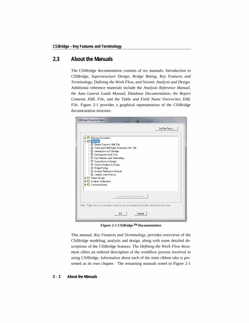
The CSiBridge documentation consists of six manuals: Introduction to CSIBridge, Superstructure Design, Bridge Rating, Key Features and Terminology, Defining the Work Flow, and Seismic Analysis and Design. Additional reference materials include the Analysis Reference Manual, the Auto Lateral Loads Manual, Database Documentation, the Report Contents XML File, and the Table and Field Name Overwrites XML File. Figure 2-1 provides a graphical representation of the CSiBridge documentation structure.
Figure 2-1 CSiBridge Documentation
This manual, Key Features and Terminology, provides overviews of the CSiBridge modeling, analysis and design. along with some detailed de-scriptions of the CSiBridge features. The Defining the Work Flow docu-ment offers an ordered description of the workflow process involved in using CSiBridge. Information about each of the main ribbon tabs is pre-sented as its own chapter. The remaining manuals noted in Figure 2-1
2 - 2 About the Manuals
Chapter 2 Getting Started
describe how to create a bridge model, analyze the model, and design or rate the superstructure. Information covering the design theory and methods, in accordance with various AASHTO design codes, is provided in the Superstructure Design, Bridge Rating and the Seismic Design manuals.
It is strongly recommended that users read this and the others manuals and view the tutorial movies (see “Watch & Learn Movies”) before at-tempting to complete a project using CSiBridge.
Additional information can be found in the Help facility that is accessi-ble using the File > Resources > Help > Show command.
2.4 “Watch & Learn™ Movies”
One of the best resources available for learning about the CSiBridge program is the “Watch & Learn” movie series, which may be accessed via the CSI website at https://www.csiamerica.com. These movies con-tain a wealth of information for both the first-time user and the experi-enced expert, covering a wide range of topics from basic operation to complex modeling. The movies range from a few minutes to more than a half hour in length.
2.5 CSI Knowledge Base
CSI maintains a knowledge base containing answers to frequently asked support questions as well as additional insights on program operation. This is a good first stop before contacting technical support because many of the most common, as well as some esoteric questions are an-swered here. This page is fully indexed and searchable, and may be found at https://wiki.csiamerica.com.
“Watch & Learn™ Movies” 2 - 3
CSiBridge – Key Features and Terminology
2.6 Technical Support
If you have questions regarding use of the software, please:
Consult the documentation and other printed information included with your product.
Check the on-line Help facility in the software.
Visit the CSI Knowledge Base at https://wiki.csiamerica.com.
If you have a current Maintenance Agreement you may request support in one of the following ways:
Send an email and your model file to [email protected] or your local CSI Partner.
Visit CSI’s website and Customer Support Portal at https://www.csiamerica.com.
Call CSI or your local CSI Partner. Contact details are available at https://www.csiamerica.com/contact.
Be sure to include the necessary information listed in the ‘Help Us to Help You’ section whenever you contact technical support.
2.7 Help Us to Help You
Whenever you contact us with a technical support question, please pro-vide us with the following information to help us help you:
The product level (Plus, Plus w/Rating, Advanced, or Advanced w/Rating) and version number that you are using. This can be ob-tained from inside the software using the File > Resource > Help > About CSiBridge command.
A description of your model, including a picture, if possible.
A description of what happened and what you were doing when the problem occurred.
The exact wording of any error messages that appeared on your screen.
A description of how you tried to solve the problem.
2 - 4 Technical Support

Chapter 2 Getting Started
The computer configuration (make and model, processor, operating system, hard disk size, and RAM size).
Your name, your company’s name, and how we may contact you.
If calling, please be at your computer where you can run the soft-ware.
Help Us to Help You 2 - 5
Chapter 3 Lanes
The vehicle live loads are considered to act in traffic lanes transversely spaced across the bridge roadway. The number of lanes and their trans-verse spacing can be chosen to satisfy the appropriate design-code re-quirements. For simple bridges with a single roadway, the lanes will usually be parallel and evenly spaced, and will run the full length of the bridge structure.
For complex structures, such as interchanges, multiple roadways may be considered; these roadways can merge and split. Lanes need not be par-allel or of the same length. The number of lanes across the roadway may vary along the length to accommodate merges. Multiple patterns of lanes on the same roadway may be created to examine the effect of different lateral placement of vehicles.
3.1 Centerline and Direction
A traffic lane is defined with respect to a reference line, which can be a bridge layout line or a line (path) of frame elements. The transverse posi-tion of the lane centerline is specified by its eccentricity relative to the reference line. Lanes are said to “run” in a particular direction, namely from the first location on the reference line used to define the lane to the last.
Centerline and Direction 3 - 1
CSiBridge – Key Features and Terminology
3.2 Eccentricity
Each lane across the roadway width will usually refer to the same refer-ence line, but will typically have a different eccentricity. The eccentricity for a given lane may also vary along the lane length.
The sign of a lane eccentricity is defined as follows: in an elevation view of the bridge where the lane runs from left to right, lanes located in front of the roadway elements have positive eccentricity. Alternatively, to a driver traveling on the roadway in the direction that the lane runs, a lane to the right of the reference line has a positive eccentricity. The best way to check eccentricities is to view them graphically in the graphical user interface.
In a spine model, the use of eccentricities is primarily important for the determination of torsion in the bridge deck and transverse bending in the substructure. In shell and solid models of the superstructure, the eccen-tricity determines where the load is applied on the deck.
3.3 Width
A width can be specified for each lane, which may be constant or varia-ble along the length of the lane. When a lane is wider than a vehicle, each axle or distributed load of the vehicle will be moved transversely in the lane to maximum effect. If the lane is narrower than the vehicle, the vehicle is centered on the lane and the vehicle width is reduced to the width of the lane.
3.4 Interior and Exterior Edges
Certain AASHTO vehicles require that the wheel loads maintain a speci-fied minimum distance from the edge of the lane. This distance may be different depending on whether the edge of the lane is at the edge of the roadway or is interior to the roadway. For each lane, the left and right edges can be specified as interior or exterior, with interior being the de-fault. This affects only vehicles that specify minimum distances for the
3 - 2 Eccentricity
Chapter 3 Lanes
wheel loads. By default, vehicle loads may be placed transversely any-where in the lane, i.e., the minimum distance is zero. Left and right edg-es are as they would be viewed by a driver traveling in the direction the lane runs.
3.5 Discretization
An influence surface will be constructed for each lane for the purpose of placing the vehicles to maximum effect. This surface is interpolated from unit point loads, called influence loads, placed along the width and length of the lane. Using more influence loads increases the accuracy of the analysis at the expense of more computational time, memory, and disk storage.
The number of influence loads can be controlled by independently speci-fying the discretization to be used along the length and across the width of each lane. Discretization is given as the maximum distance allowed between load points. Transversely, it is usually sufficient to use half the lane width, resulting in load points at the left, right, and center of the lane. Along the length of the lane, using eight to sixteen points per span is often adequate.
As with analyses of any type, it is strongly recommended that initially the model be set up to run quickly by using a coarser discretization. As experience is gained with the model, reality checks should be used to evaluate if further discretization is appropriate. If so, the discretization can be refined to achieve the desired level of accuracy and detailed re-sults.
Discretization 3 - 3
Chapter 4 Influence Lines and Surfaces
4.1 Overview
CSiBridge uses influence lines and surfaces to compute the response to vehicle live loads. Influence lines and surfaces are also of interest in their own right for understanding the sensitivity of various response quantities to traffic loads.
Influence lines are computed for lanes of zero width, while influence surfaces are computed for lanes having finite width.
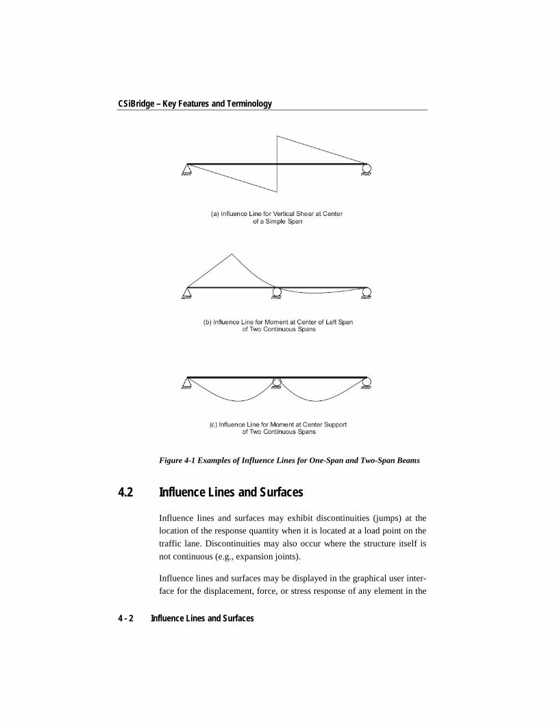
An influence line can be viewed as a curve of influence values plotted at the load points along a traffic lane. For a given response quantity (force, displacement, or stress) at a given location in the structure, the influence value plotted at a load point is the value of that response quantity for a unit of concentrated downward force acting at that load point. The influ-ence line thus shows the influence upon the given response quantity of a unit force moving along the traffic lane. Figure 4-1 shows some simple examples of influence lines. An influence surface is the extension of this concept into two dimensions across the width of the lane.
Overview 4 - 1
CSiBridge – Key Features and Terminology
Figure 4-1 Examples of Influence Lines for One-Span and Two-Span Beams
4.2 Influence Lines and Surfaces
Influence lines and surfaces may exhibit discontinuities (jumps) at the location of the response quantity when it is located at a load point on the traffic lane. Discontinuities may also occur where the structure itself is not continuous (e.g., expansion joints).
Influence lines and surfaces may be displayed in the graphical user inter-face for the displacement, force, or stress response of any element in the
4 - 2 Influence Lines and Surfaces

Chapter 4 Influence Lines and Surfaces
structure. They are plotted on the lanes with the influence values plotted in the vertical direction. A positive influence value due to gravity load is plotted upward. Influence values are linearly interpolated between the known values at the load points.
Influence Lines and Surfaces 4 - 3
Chapter 5 Vehicle Live Loads
Any number of vehicle live loads, or simply vehicles, may be defined to act on the traffic lanes. Standard types of vehicles known to the program can be used, or the general vehicle specification can be used to tailor de-sign of vehicles types.
5.1 Direction of Loading
All vehicle live loads represent weight and are assumed to act down-ward, in the –Z global coordinate direction.
5.2 Distribution of Loads
Longitudinally, each vehicle consists of one or more axle loads and/or one or more uniform loads. Axle loads act at a single longitudinal loca-tion in the vehicle. Uniform loads may act between pairs of axles, or ex-tend infinitely before the first axle or after the last axle. The width of each axle load and each uniform load is independently specified. These widths may be fixed or equal to the width of the lane.
Direction of Loading 5 - 1
CSiBridge – Key Features and Terminology
For moving-load load cases using the influence surface, both axle loads and uniform loads are used to maximum effect. For step-by-step analy-sis, only the axle loads are used.
5.3 Axle Loads
Longitudinally, axle loads look like a point load. Transversely, axle loads may be represented as one or more point (wheel) loads or as dis-tributed (knife-edge) loads. Knife-edge loads may be distributed across a fixed width or the full width of the lane. Axle loads may be zero, which can be used to separate uniform loads of different magnitude.
5.4 Uniform Loads
Longitudinally, the uniform loads are constant between axles. Leading and trailing loads may be specified that extend to infinity. Transversely, these loads may be distributed uniformly across the width of the lane, over a fixed width, or they may be concentrated at the center line of the lane.
5.5 Minimum Edge Distances
Certain AASHTO vehicles require that the wheel loads maintain a speci-fied minimum distance from the edge of the lane. For any vehicle, you may specify a minimum distance for interior edges of lanes, and another distance for exterior edges. By default, these distances are zero. The specified distances apply equally to all axle loads, but do not affect lon-gitudinally uniform loads. For design purposes and the calculation of the live load distribution factors and other vehicle load effects, the user must specify the edge curb locations when specifying the bridge section data.
5 - 2 Axle Loads
Chapter 5 Vehicle Live Loads
5.6 Restricting a Vehicle to the Lane Length
When moving a vehicle along the length of the lane, the front of the ve-hicle starts at one end of the lane, and the vehicle travels forward until the back of the vehicle exits the other end of the lane. This means that all locations of the vehicle are considered, whether fully or partially on the lane
An option can be used to specify that a vehicle must remain fully on the lane. This is useful for cranes and similar vehicles that have stops at the end of their rails that prevent them from leaving the lane. This setting af-fects only influence-surface analysis, not step-by-step analysis where the vehicle runs can be explicitly controlled.
5.7 Application of Loads to the Influence Surface
The maximum and minimum values of a response quantity are computed using the corresponding influence line or surface. Concentrated loads are multiplied by the influence value at the point of application to obtain the corresponding response; distributed loads are multiplied by the influence values and integrated over the length and width of application.
By default, each concentrated or distributed load is considered to repre-sent a range of values from zero up to a specified maximum. When com-puting a response quantity (force or displacement), the maximum value of load is used where it increases the severity of the response, and zero is used where the load would have a relieving effect. Thus the specified load values for a given vehicle may not always be applied proportional-ly. This is a conservative approach that accounts for vehicles that are not fully loaded. Thus the maximum response is always positive (or zero); the minimum response is always negative (or zero).
This conservative behavior can be overridden, as explained in the next subsection, “Option to Allow Reduced Response Severity”.
By way of example, consider the influence line for the moment at the center of the left span shown in Figure 4-1 in Chapter 4. Any axle load
Restricting a Vehicle to the Lane Length 5 - 3
CSiBridge – Key Features and Terminology
or portion of a distributed load that acts on the left span would contribute only to the positive maximum value of the moment response. Loads act-ing on the right span would not decrease this maximum, but would con-tribute to the negative minimum value of this moment response.
5.7.1 Option to Allow Reduced Response Severity An option is available to allow loads to reduce the severity of the re-sponse. When this option is used, all concentrated and uniform loads will be applied at full value on the entire influence surface, whether that load reduces the severity of the response or it does not. This is less conserva-tive than the default method of load application. This option may be use-ful for routing special vehicles whose loads are well known. However, for notional loads that represent a distribution or envelope of unknown vehicle loadings, the default method may be more appropriate.
5.7.2 Width Effects Fixed-width loads will be moved transversely across the width of a lane for maximum effect if the lane is wider than the load. If the lane is nar-rower than the load, the load will be centered on the lane and its width reduced to be equal to that of the lane, keeping the total magnitude of the load unchanged.
The load at each longitudinal location in the vehicle is independently moved across the width of the lane. This means that the front, back, and middle of the vehicle may not occupy the same transverse location in the lane when placed for maximum effect.
5.8 Length Effects
The magnitude of the loading can be specified to depend on lane length using built-in or user-defined length functions. One function may be used to affect the concentrated (axle) loads, and another function may be used for the distributed loads. These functions act as scale factors on the specified load values.
5 - 4 Length Effects
Chapter 5 Vehicle Live Loads
5.8.1 Concentrated (Axle) Loads If a length-effect function is specified for the axle loads, all axle loads will be scaled equally by the function, including floating axle loads. Built-in length-effect functions include the AASHTO Standard Impact function and the JTG-D60 Lane load function. Users may also define their own functions.
The intent of this function is to scale the load according to span length. In a given structure, there may not be a constant span length, so the pro-gram uses the influence line to determine what span length to use. This may differ for each computed response quantity, and may not always correspond to the obvious span length in the global structure.
For a given response quantity, the maximum point on the influence line is found, and the distance between the zero-crossings on either side of this maximum is taken to be the span length. For the three influence lines of Figure 4-1 in Chapter 4, this would result in a span length of half the distance between the supports for the shear in (a), and the full distance between the supports for the moments in (b) and (c). For shear near the support, the span length would be essentially the same as the distance between the supports.
This approach generally works well for moments and for shear near the supports. A shorter span length is computed for shear near midspan, but here the shear is smaller anyway, so it is not usually of concern.
5.8.2 Distributed Loads If a length-effect function is specified for the distributed loads, all dis-tributed loads will be scaled equally by the function. Built-in length-effect functions include the AASHTO Standard Impact function and the British HA function. Users may also define their own functions.
The intent of this function is to scale the load according to the loaded length, but not unconservatively. The influence line is used to determine the loaded length for each individual response quantity. Only loaded lengths that increase the severity of the response are considered.
Length Effects 5 - 5
CSiBridge – Key Features and Terminology
To prevent long lengths of small influence from unconservatively reduc-ing the response, an iterative approach is used where the length consid-ered is progressively increased until the maximum response is computed. Any further increases in length that reduce the response due to decreas-ing function value are ignored.
5.9 Application of Loads in Multi-Step Analysis
Vehicles can be moved in a multi-step analysis. This can use multi-step static load cases or time-history load cases, the latter of which can be linear or nonlinear.
Influence surfaces are not used for this type of analysis. Rather, CSiBridge creates many internal load patterns representing different po-sitions of the vehicles along the length of the lanes.
Only axle loads are considered; the uniform loads are not applied. In the case of variable axle spacing, the minimum distance is used. The trans-verse distribution of the axle loads is considered. The vehicle is moved longitudinally along the centerline of the lane; it is not moved trans-versely within the lane. Additional lanes can be defined to consider dif-ferent transverse positions.
The full magnitude of the loads is applied, whether they increase or de-crease the severity of the response. Each step in the analysis corresponds to a specific position of each vehicle acting in its lane. All response at that step is fully correlated.
5 - 6 Application of Loads in Multi-Step Analysis
Chapter 6 General Vehicle
The general vehicle may represent an actual vehicle or a notional vehicle used by a design code. Most trucks and trains can be modeled by the CSiBridge general vehicle.
The general vehicle consists of axles with specified distances between them. Concentrated loads may exist at the axles. Uniform loads may ex-ist between pairs of axles, in front of the first axle, and behind the last axle. The distance between any one pair of axles may vary over a speci-fied range; the other distances are fixed. The leading and trailing uniform loads are of infinite extent. Additional “floating” concentrated loads may be specified that are independent of the position of the axles.
By default for influence surface analysis, applied loads never decrease the severity of the computed response, so the effect of a shorter vehicle is captured by a longer vehicle that includes the same loads and spacings as the shorter vehicle. Only the longer vehicle need be considered in such cases.
If the option to allow loads to reduce the severity of response is chosen, both the shorter and longer vehicles must be considered, if they both ap-ply. This is also true for step-by-step analysis.
Specification 6 - 1
CSiBridge – Key Features and Terminology
6.1 Specification
To define a vehicle, the following may be specified:
n–1 positive distances, d, between the pairs of axles; one inter-axle distance may be specified as a range from dmin to dmax, where 0 < dmin ≤ dmax, and dmax = 0 can be used to represent a maximum distance of infinity
n concentrated loads, p, at the axles, including the transverse load distribution for each
n+1 uniform loads, w: the leading load, the inter-axle loads, and the trailing load, including the transverse load distribution for each
Floating axle loads:
– Load pm for superstructure moments, including its transverse distribution; this load can be doubled for negative superstruc-ture moments over the supports, as described in the next bullet item
– Load pxm for all response quantities except superstructure moments, including its transverse distribution
Use or do not use this vehicle for calculating:
– “Negative” superstructure moments over the supports
– Reaction forces at interior supports
– Response quantities other than the preceding two types
Minimum distances between the axle loads and the edges of the lane; by default these distances are zero
The vehicle does or does not remain fully within the length of the lane.
The magnitude of the uniform loads is or is not automatically re-duced based on the loaded length of the lane in accordance with the British code.
The number of axles, n, may be zero, in which case only a single uni-form load and the floating concentrated loads can be specified.
6 - 2 Specification
Chapter 6 General Vehicle
6.2 Moving the Vehicle
When a Vehicle is applied to a traffic lane, the axles are moved along the length of the lane to where the maximum and minimum values are pro-duced for every response quantity in every element. Usually this location will be different for each response quantity. For asymmetric (front to back) vehicles, both directions of travel are considered.
Moving the Vehicle 6 - 3
Chapter 7 Vehicle Response Components
Certain features of the AASHTO H, HS, and HL vehicular live loads (AASHTO 2007) apply only to certain types of bridge response, such as negative moment in the superstructure or the reactions at interior sup-ports. CSiBridge uses the concept of vehicle response components to identify these response quantities. In these cases, objects that need spe-cial treatment should be selected, and appropriate vehicle response com-ponents should be assigned to them.
The different types of available vehicle response components are de-scribed in the following subtopics.
7.1 Superstructure (Span) Moment
For AASHTO H and HS “Lane” loads, the floating axle load pm is used for calculating the superstructure moment. How this moment is repre-sented depends on the type of model used. For all other types of re-sponse, the floating axle load pxm is used.
The general procedure is to select the elements representing the super-structure and assign vehicle response components “H and HS Lane Loads – Superstructure Moment” to the desired response quantities, as described next.
Superstructure (Span) Moment 7 - 1
CSiBridge – Key Features and Terminology
For a spine (spline) model where the superstructure is modeled as a line of frame elements, superstructure moment corresponds to frame moment M3 for elements where the local-2 axis is in the vertical plane (the de-fault.) Thus all frame elements representing the superstructure would be selected and assigned the vehicle response components to M3, indicating to “Use All Values” (i.e., positive and negative.) Load pm will be used for computing M3 of these elements.
For a full-shell model of the superstructure, superstructure moment cor-responds to longitudinal stresses or membrane forces in the shell ele-ments. Assuming the local-1 axes of the shell elements are oriented along the longitudinal direction of the bridge, all shell elements repre-senting the superstructure would be selected and assigned the vehicle re-sponse components to S11 and/or F11, indicating to “Use All Values” (i.e., positive and negative). This same assignment could also be made to shell moments M11. Load pm will be used for computing any compo-nents so assigned.
7.2 Negative Superstructure (Span) Moment
For AASHTO H and HS “Lane” loads, the floating axle load pm is ap-plied in two adjacent spans for calculating the negative superstructure moment over the supports. Similarly, for AASHTO HL loads, a special double-truck vehicle is used for calculating negative superstructure mo-ment over interior supports. Negative moment here means a moment that causes tension in the top of the superstructure, even if the sign of the CSiBridge response is positive for a particular choice of local axes.
The procedure for different types of structures is very similar to that de-scribed previously for superstructure moment: select the elements repre-senting the superstructure, but now assign vehicle response components “H, HS and HL Lane Loads – Superstructure Negative Moment over Supports” to the desired response quantities. However, a decision must be made about how to handle the sign.
There are two general approaches. Consider the case of the spine model with frame moment M3 representing superstructure moment:
7 - 2 Negative Superstructure (Span) Moment
Chapter 7 Vehicle Response Components
(1) The entire superstructure can be selected and assigned the vehicle response components to M3, indicating to “Use Negative Values.” Only negative values of M3 will be computed using the double pm or double-truck load.
(2) Only that part of the superstructure within a pre-determined nega-tive-moment region, such as between the inflection points under dead load, could be selected. Assign the vehicle response compo-nents to M3, indicating to “Use Negative Values” or “Use All Val-ues.”
The first approach may be slightly more conservative, giving negative moments over a larger region. However, it does not require that a nega-tive-moment region be determined.
The situation with the shell model is more complicated, since negative moments correspond to positive membrane forces and stresses at the top of the superstructure, negative values at the bottom of the superstructure, and changing sign in between. For this reason, the preceding approach (2) may be better: determine a negative-moment region, then assign the vehicle response components to the desired shell stresses, membrane forces, and/or moments, indicating to “Use All Values.” This avoids the problem of sign where it changes through the depth.
7.3 Reactions at Interior Supports
For AASHTO HL loads, a special double-truck vehicle is used for calcu-lating the reactions at interior supports. It is up to the user to determine what response components is to be used to compute for this purpose. Choices could include:
Vertical upward reactions, or all reactions, for springs and restraints at the base of the columns
Compressive axial force, or all forces and moments, in the columns
Compressive axial force, or all forces and moments, in link elements representing bearings
Reactions at Interior Supports 7 - 3
CSiBridge – Key Features and Terminology
Bending moments in outriggers at the columns
The preceding procedure is for superstructure moment. Select the ele-ments representing the interior supports and assign the vehicle response components “HL – Reactions at Interior Supports” to the desired re-sponse quantities. Carefully decide if all values, or only negative or posi-tive values, are to be used. This process will need to be repeated for each type of element that is part of the interior supports: joints, frames, links, shells, and/or solids.
7 - 4 Reactions at Interior Supports
Chapter 8 Standard Vehicles
Many standard vehicles are available in CSiBridge to represent vehicular live loads specified in various design codes. More are being added all the time. A few examples are provided here for illustrative purposes. Only the longitudinal distribution of loading is shown in the figures. Please see the graphical user interface for all available types and further infor-mation.
8.1 Hn-44 and HSn-44
Vehicles specified with type = Hn-44 and type = HSn-44 represent the AASHTO standard H and HS Truck Loads, respectively. The n in the type is an integer scale factor that specifies the nominal weight of the vehicle in tons. Thus H15-44 is a nominal 15 ton H Truck Load, and HS20-44 is a nominal 20 ton HS Truck Load.
The effect of an H Vehicle is included in an HS Vehicle of the same nominal weight. If the structure is being designed for both H and HS ve-hicles, only the HS Vehicle is needed.
Hn-44 and HSn-44 8 - 1
CSiBridge – Key Features and Terminology
8.2 Hn-44L and HSn-44L
Vehicles specified with type = Hn-44L and type = HSn-44L represent the AASHTO standard H and HS Lane Loads, respectively. The n in the type is an integer scale factor that specifies the nominal weight of the vehicle in tons. Thus H15-44 is a nominal 15-ton H Lane Load, and HS20-44 is a nominal 20-ton HS Lane Load. The Hn-44L and HSn-44L Vehicles are identical.
8.3 AML
Vehicles specified with type = AML represent the AASHTO standard Alternate Military Load. This vehicle consists of two 24-kip axles spaced 4 feet apart.
8.4 HL-93K, HL-93M, and HL-93S
Vehicles specified with type = HL-93K represent the AASHTO standard HL-93 Load, consisting of the code-specified design truck and the de-sign lane load.
Vehicles specified with type = HL-93M represent the AASHTO standard HL-93 Load, consisting of the code-specified design tandem and the de-sign lane load.
Vehicles specified with type = HL-93S represent the AASHTO standard HL-93 Load, consisting of two code-specified design trucks and the de-sign lane load, all scaled by 90%. The axle spacing for each truck is fixed at 14 feet. The spacing between the rear axle of the lead truck and the lead axle of the rear truck varies from 50 feet to the length of the lane. This vehicle is only used for negative superstructure moment over supports and reactions at interior supports. The response will be zero for all response quantities that do not have the appropriately assigned vehi-cle response components.
8 - 2 Hn-44L and HSn-44L

Chapter 8 Standard Vehicles
A dynamic load allowance may be specified for each vehicle using the parameter im. This is the additive percentage by which the concentrated truck or tandem axle loads will be increased. The uniform lane load is not affected. Thus if im = 33, all concentrated axle loads for the vehicle will be multiplied by the factor 1.33.
8.5 P5, P7, P9, P11, and P13
Vehicles specified with type = P5, type = P7, type = P9, type = P11, and type = P13 represent the Caltrans standard Permit Loads.
The effect of a shorter Caltrans Permit Load is included in any of the longer Permit Loads. When designing for all of these permit loads, only the P13 Vehicle is needed.
8.6 Cooper E 80
Vehicles specified with type = COOPERE80 represent the AREA stand-ard Cooper E 80 train load.
8.7 UICn
Vehicles specified with type = UICn represent the European UIC (or British RU) train load. The n in the type is an integer scale factor that specifies magnitude of the uniform load in kN/m. Thus UIC80 is the full UIC load with an 80 kN/m uniform load, and UIC60 is the UIC load with an 60 kN/m uniform load. The concentrated loads are not affected by n.
8.8 RL
Vehicles specified with type = RL represent the British RL train load.
P5, P7, P9, P11, and P13 8 - 3
Chapter 9 Vehicle Classes
9.1 Vehicle Class Definitions
The designer is often interested in the maximum and minimum response of the bridge to the most extreme of several types of vehicles rather than the effect of the individual vehicles. For this purpose, vehicle classes are defined that may include any number of individual vehicles. The maxi-mum and minimum force and displacement response quantities for a ve-hicle class will be the maximum and minimum values obtained for any individual vehicle in that class. Only one vehicle ever acts at a time.
For influence-based analyses, all vehicle loads are applied to the traffic lanes through the use of vehicle classes. If it is desired to apply an indi-vidual vehicle load, a vehicle class that contains only that single vehicle must be defined. For step-by-step analysis, vehicle loads are applied di-rectly without the use of classes, since no enveloping is performed.
For example, it may be necessary to consider the most severe of a truck load and the corresponding lane load, such as the HS20-44 and HS20-44L loads. A vehicle class can be defined to contain these two vehicles. additional vehicles, such as the Alternate Military Load type AML, could be included in the class as appropriate. Different members of the
Vehicle Class Definitions 9 - 1

CSiBridge – Key Features and Terminology
class may cause the most severe response at different locations in the structure.
For HL-93 loading, first define three vehicles, one each of the standard types HL-93K, HL-93M, and HL-93S. Then a single vehicle class con-taining all three vehicles could be defined.
9 - 2 Vehicle Class Definitions
Chapter 10 Moving Load Load Cases
The final step in the definition of the influence-based vehicle live load-ing is the application of the vehicle classes to the traffic lanes. This is accomplished by creating independent moving-load load cases.
A moving load load case is a type of load case. Unlike most other load cases, load patterns can not be applied in a moving load load case. In-stead, each moving load load case consists of a set of assignments that specify how the classes are assigned to the lanes.
Each assignment in a moving load load case requires the following data:
A vehicle class
A scale factor multiplying the effect of the class (the default is uni-ty)
A list of one or more lanes in which the class may act (the default is all lanes)
The minimum number of lanes in which the class must act (the de-fault is zero)
The maximum number of lanes in which the class may act (the de-fault is all of lanes)
10 - 1
CSiBridge – Key Features and Terminology
The program looks at all of the assignments in a moving-load load case and tries every possible permutation of loading the traffic lanes with ve-hicle classes that is permitted by the assignments. No lane is ever loaded by more than one class at a time.
Multiple-lane scale factors (rf1, rf2, rf3, and so on) that multiply the ef-fect of each permutation depending upon the number of loaded lanes can be specified for each moving-load load case. For example, the effect of a permutation that loads two lanes is multiplied by rf2.
The maximum and minimum response quantities for a moving-load load case will be the maximum and minimum values obtained for any permu-tation permitted by the assignments. Usually the permutation producing the most severe response will be different for different response quanti-ties.
The concepts of assignment can be clarified with the help of the follow-ing examples.
10.1 AASHTO HS Loading
Consider a four-lane bridge designed to carry AASHTO HS20-44 Truck and Lane Loads, and the Alternate Military Load (AASHTO, 1996). As-sume that it is required that the number of lanes loaded be that which produces the most severe response in every member. Only one of the three vehicle loads is allowed per lane. Load intensities may be reduced by 10% and 25% when three or four lanes are loaded, respectively.
Generally, loading all of the lanes will produce the most severe moments and shears along the span and axial forces in the piers. However, the most severe torsion of the bridge deck and transverse bending of the piers will usually be produced by loading only those lanes possessing eccentricities of the same sign.
Assume that the bridge structure and traffic lanes have been defined. Three vehicles are defined:
10 - 2 AASHTO HS Loading
Chapter 10 Moving Load Load Cases
name = HSK, type = HS20-44
name = HSL, type = HS20-44L
name = AML, type = AML
where name is an arbitrary label assigned to each vehicle. The three ve-hicles are assigned to a single vehicle class, with an arbitrary label of name = HS, so that the most severe of these three vehicle loads will be used for every situation.
A single moving-load load case is then defined that seeks the maximum and minimum responses throughout the structure for the most severe loading of all four lanes, any three lanes, any two lanes or any single lane. This can be accomplished using a single assignment. The parame-ters for the assignment are:
class = HS
sf = 1
lanes = 1, 2, 3, 4
lmin = 1
lmax = 4
The scale factors for the loading of multiple lanes in the set of assign-ments are rf1 = 1, rf2 = 1, rf3 = 0.9, and rf4 = 0.75.
There are fifteen possible permutations assigning the single vehicle class HS to any one, two, three, or four lanes. These are presented in the table that follow.
An “HS” in a lane column of the table indicates application of Class HS; a blank indicates that the lane is unloaded. The scale factor for each permutation is determined by the number of lanes loaded.
AASHTO HS Loading 10 - 3
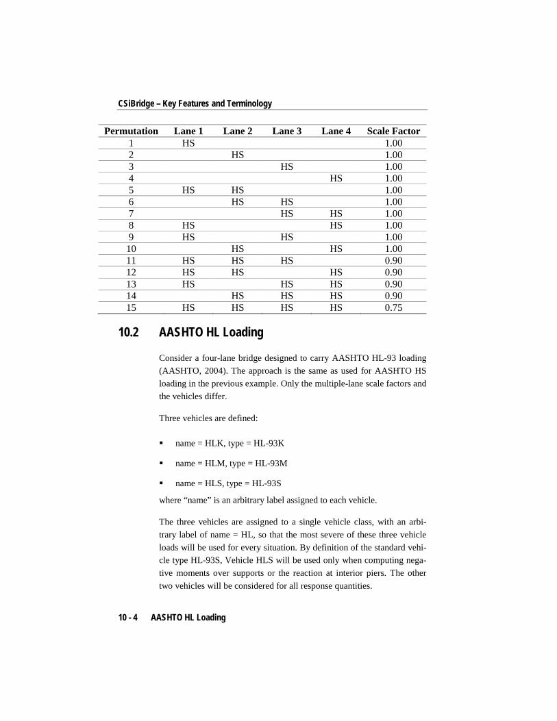
CSiBridge – Key Features and Terminology
Permutation Lane 1 Lane 2 Lane 3 Lane 4 Scale Factor 1 HS 1.00 2 HS 1.00 3 HS 1.00 4 HS 1.00 5 HS HS 1.00 6 HS HS 1.00 7 HS HS 1.00 8 HS HS 1.00 9 HS HS 1.00
10 HS HS 1.00 11 HS HS HS 0.90 12 HS HS HS 0.90 13 HS HS HS 0.90 14 HS HS HS 0.90 15 HS HS HS HS 0.75
10.2 AASHTO HL Loading
Consider a four-lane bridge designed to carry AASHTO HL-93 loading (AASHTO, 2004). The approach is the same as used for AASHTO HS loading in the previous example. Only the multiple-lane scale factors and the vehicles differ.
Three vehicles are defined:
name = HLK, type = HL-93K
name = HLM, type = HL-93M
name = HLS, type = HL-93S
where “name” is an arbitrary label assigned to each vehicle.
The three vehicles are assigned to a single vehicle class, with an arbi-trary label of name = HL, so that the most severe of these three vehicle loads will be used for every situation. By definition of the standard vehi-cle type HL-93S, Vehicle HLS will be used only when computing nega-tive moments over supports or the reaction at interior piers. The other two vehicles will be considered for all response quantities.
10 - 4 AASHTO HL Loading
Chapter 10 Moving Load Load Cases
A single moving-load load case is then defined that is identical to that of the previous example, except that class = HL, and the scale factors for multiple lanes are rf1 = 1.2, rf2 = 1, rf3 = 0.85, and rf4 = 0.65.
There are again fifteen possible permutations assigning the single vehi-cle class HL to any one, two, three, or four lanes. These are similar to the permutations of the previous example, with the scale factors changed as appropriate.
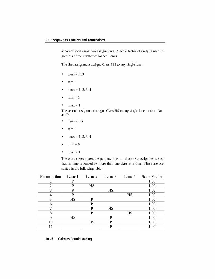
10.3 Caltrans Permit Loading
Consider the four-lane bridge of the previous examples now subject to Caltrans Combination Group (Caltrans 1995). Here the permit load(s) is to be used alone in a single traffic lane, or in combination with one HS or Alternate Military Load in a separate traffic lane, depending upon which is more severe.
Four vehicles are defined:
name = HSK, type = HS20-44
name = HSL, type = HS20-44L
name = AML, type = AML
name = P13, type = P13
where name is an arbitrary label assigned to each vehicle.
The first three vehicles are assigned to a vehicle class that is given the label name = HS, as in the first example (Section 10.1). The last vehicle is assigned as the only member of a vehicle class that is given the label name = P13. Note that the effects of CSiBridge vehicle types P5, P7, P9, and P11 are captured by vehicle type P13.
Combination Group is then represented as a single moving-load load case consisting of the assignment of Class P13 to any single lane with or without Class HS being assigned to any other single lane. This can be
Caltrans Permit Loading 10 - 5
CSiBridge – Key Features and Terminology
accomplished using two assignments. A scale factor of unity is used re-gardless of the number of loaded Lanes.
The first assignment assigns Class P13 to any single lane:
class = P13
sf = 1
lanes = 1, 2, 3, 4
lmin = 1
lmax = 1 The second assignment assigns Class HS to any single lane, or to no lane at all:
class = HS
sf = 1
lanes = 1, 2, 3, 4
lmin = 0
lmax = 1
There are sixteen possible permutations for these two assignments such that no lane is loaded by more than one class at a time. These are pre-sented in the following table:
Permutation Lane 1 Lane 2 Lane 3 Lane 4 Scale Factor 1 P 1.00 2 P HS 1.00 3 P HS 1.00 4 P HS 1.00 5 HS P 1.00 6 P 1.00 7 P HS 1.00 8 P HS 1.00 9 HS P 1.00
10 HS P 1.00 11 P 1.00
10 - 6 Caltrans Permit Loading
Chapter 10 Moving Load Load Cases
Permutation Lane 1 Lane 2 Lane 3 Lane 4 Scale Factor 12 P HS 1.00 13 HS P 1.00 14 HS P 1.00 15 HS P 1.00 16 P 1.00
10.4 Restricted Caltrans Permit Loading
Consider the four-lane bridge and the Caltrans permit loading of the third example (Section 10.3), but subject to the following restrictions:
The permit vehicle is allowed in lane 1 or lane 4 only.
The lane adjacent to the lane occupied by the permit vehicle must be empty.
Two moving-load load cases are required, each containing two assign-ments. A scale factor of unity is used regardless of the number of loaded lanes.
The first moving-load load case considers the case where the permit ve-hicle occupies lane 1. The first assignment assigns Class P13 to lane 1
class = P13
sf = 1
lanes = 1
lmin = 1
lmax = 1
The second assignment assigns Class HS to either lane 3 or 4, or to no lane at all:
class = HS
sf = 1
lanes = 3, 4
Restricted Caltrans Permit Loading 10 - 7
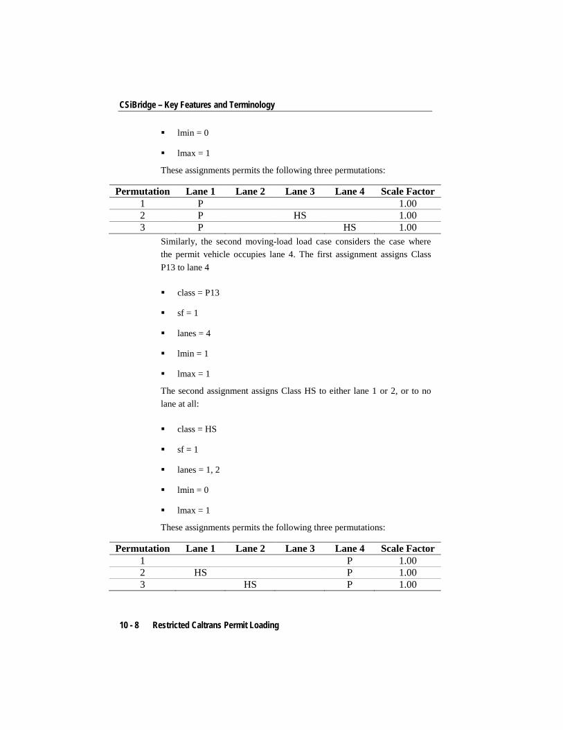
CSiBridge – Key Features and Terminology
lmin = 0
lmax = 1
These assignments permits the following three permutations:
Permutation Lane 1 Lane 2 Lane 3 Lane 4 Scale Factor 1 P 1.00 2 P HS 1.00 3 P HS 1.00
Similarly, the second moving-load load case considers the case where the permit vehicle occupies lane 4. The first assignment assigns Class P13 to lane 4
class = P13
sf = 1
lanes = 4
lmin = 1
lmax = 1
The second assignment assigns Class HS to either lane 1 or 2, or to no lane at all:
class = HS
sf = 1
lanes = 1, 2
lmin = 0
lmax = 1
These assignments permits the following three permutations:
Permutation Lane 1 Lane 2 Lane 3 Lane 4 Scale Factor 1 P 1.00 2 HS P 1.00 3 HS P 1.00
10 - 8 Restricted Caltrans Permit Loading
Chapter 10 Moving Load Load Cases
An envelope-type combo that includes only these two moving-load load cases would produce the most severe response for the six permutations above.
See “Define Loads and Load Combinations” chapter in the Superstruc-ture Design manual for more information.
Restricted Caltrans Permit Loading 10 - 9
Chapter 11 Moving Load Response Control
Several parameters are available for controlling influence-based moving load load cases. These have no effect on step-by-step analysis.
11.1 Bridge Response Groups
By default, no moving load response is calculated for any joint or ele-ment, since this calculation is computationally intensive. The user must explicitly request the moving load response to be calculated.
For each of the following types of response, a group of elements for which the response should be calculated may be requested:
Joint displacements
Joint reactions
Frame forces and moments
Shell stresses
Shell resultant forces and moments
Plane stresses
Solid stresses
Link/support forces and deformations
Bridge Response Groups 11 - 1
CSiBridge – Key Features and Terminology
If the displacements, reactions, spring forces, or internal forces are not calculated for a given joint or frame element, no moving load response can be printed or plotted for that joint or element. Likewise, no response can be printed or plotted for any combo that contains a moving-load load case.
Additional control is available as described in the following subtopics.
11.2 Correspondence
For each maximum or minimum frame-element response quantity com-puted, the corresponding values for the other five internal force and mo-ment components may be determined. For example, the shear, moment, and torque that occur at the same time as the maximum axial force in a frame element may be computed.
Similarly, corresponding displacements, stresses, forces, and moments can be computed for any response quantity of any element type. Only the corresponding values for each joint or element are computed. To view the full corresponding state of the structure, step-by-step analysis must be used.
By default, no corresponding quantities are computed since this signifi-cantly increases the computation time for moving-load response.
11.3 Influence Line Tolerance
CSiBridge simplifies the influence lines used for response calculation in order to increase efficiency. A relative tolerance is used to reduce the number of load points by removing those that are approximately dupli-cated or that can be approximately linearly interpolated. The default val-ue of this tolerance permits response errors on the order of 0.01%. Set-ting the tolerance to zero will provide exact results to within the resolu-tion of the analysis.
11 - 2 Correspondence
Chapter 11 Moving Load Response Control
11.4 Exact and Quick Response Calculation
For the purpose of moving a vehicle along a lane, each axle is placed on every load point in turn. When another axle falls between two load points, the effect of that axle is determined by linear interpolation of the influence values. The effect of uniform loads is computed by integrating the linearly interpolated segments of the influence line. This method is exact to within the resolution of the analysis, but is computationally in-tensive if there are many load points.
A “Quick” method is available that may be much faster than the usual “Exact” method, but it may also be less accurate. The Quick method ap-proximates the influence line by using a limited number of load points in each “span.” For purposes of this discussion, a span is considered to be a region where the influence line is all positive or all negative.
The degree of approximation to be used is specified by the parameter quick, which may be any non-negative integer. The default value is quick = 0, which indicates to use the full influence line, i.e., the Exact method.
Positive values indicate increasing degrees of refinement for the Quick method. For quick = 1, the influence line is simplified by using only the maximum or minimum value in each span, plus the zero points at each end of the span. For quick = 2, an additional load point is used on either side of the maximum/minimum. Higher degrees of refinement use addi-tional load points. The number of points used in a span can be as many as 2quick+1, but not more than the number of load points available in the span for the Exact method.
It is strongly recommended that quick = 0 be used for all final analyses. For preliminary analyses, quick = 1, 2, or 3 is usually adequate, with quick = 2 often providing a good balance between speed and accuracy. The effect of parameter quick upon speed and accuracy is problem-dependent, and the user should experiment to determine the best value to use for each model.
Exact and Quick Response Calculation 11 - 3
Chapter 12 Step-By-Step Analysis
Step-by-step analysis can consider any combination of vehicles operat-ing on the lanes. Multiple vehicles can operate simultaneously, even in the same lane if desired. To begin, define a load pattern of type “Bridge Live,” in which one or more sets of the following are specified:
Vehicle type
Lane in which it is traveling
Starting position in the lane
Starting time
Vehicle speed
Direction (forward or backward, relative to the Lane direction)
Then specify a time-step size and the total number of time steps to be considered. The total duration of loading is the product of these two. To get a finer spatial discretization of loading, use smaller time steps, or re-duce the speed of the vehicles.
Loading 12 - 1
CSiBridge – Key Features and Terminology
12.1 Loading
This type of load pattern is multi-stepped. It automatically creates a dif-ferent pattern of loading for each time step. At each step, the load ap-plied to the structure is determined as follows:
The longitudinal position of each vehicle in its lane at the current time is determined from its starting position, speed and direction.
The vehicle is centered transversely in the lane.
Axle loads are applied to the bridge deck. Concentrated axles loads are applied as specified. Distributed axle loads are converted to four equivalent concentrated loads.
For each individual concentrated load, consistent joint loads are cal-culated at the corners of any loaded shell or solid element on the deck. In a spine model, a concentrated force and eccentric moment is applied to the closest frame element representing the superstruc-ture.
Variable axle spacing, if present, is fixed at the minimum distance.
Longitudinally uniform loads are not considered.
Floating axle loads are not considered.
To consider different axle spacing, define additional vehicles. To con-sider different transverse placement of the vehicles, define additional lanes.
12.2 Static Analysis
When a load pattern of type “Bridge Live” is applied in a multi-step stat-ic load case, there results a separate linear static solution step for each time step, starting at time zero. Each solution is independent, represent-ing the displacement and stress state in the structure for the current posi-tion of the vehicles. These results can be plotted in sequence, used in creating a video showing the movement of the vehicles across the struc-
12 - 2 Loading
Chapter 12 Step-By-Step Analysis
ture along with the resulting displacements and/or stresses, or enveloped for the Load Case.
Since the analysis is static, the speed of the vehicles has no effect on the results, other than determining the change in position from one load step to the next.
12.3 Time-History Analysis
When a load pattern of type “Bridge Live” is applied in a time-history load case, CSiBridge automatically creates a separate time function for each load pattern that ramps the load up from zero to one over one time step, and back down to zero in the succeeding time step. This is done re-gardless of which time function is specified. Thus at any given time within a time step, the applied load is a linear interpolation of the load pattern at the beginning and the end of the time step.
Direct integration is recommended. Modal superposition would require a very large number of modes since the spatial distribution of the load is constantly changing.
Dynamical effects are important in a time-history analysis, and different results may be expected depending on the speed of the vehicle.
The time-history load case may be linear or nonlinear. To consider static nonlinearity, perform a quasi-static nonlinear time-history analysis, i.e., at very slow speed with long time steps. The speed should be slow enough so that the time it takes to cross a span is significantly longer than the first period of the structure.
12.4 Enveloping and Load Combinations
Results for each step-by-step load case may be displayed or printed for individual steps, or as an envelope giving the maximum and minimum response. When included in load combinations, envelope results will be used.
Time-History Analysis 12 - 3
CSiBridge – Key Features and Terminology
An influence-based analysis can be approximated as follows:
Define one or more load patterns of type Bridge-Live, each of which moves a single vehicle in a single lane in a single direction
For each load pattern, create a corresponding multi-step static load case that applies only that load pattern
For each lane, define an envelope-type load combination of all load cases defined for that lane
Define a single range-type combo that includes all of the lane enve-lope-type load combinations
This procedure can be modified as needed to meet a particular applica-tion. The important thing is to be sure that in the final load combination, no lane is ever loaded by more than one vehicle at a time, unless that is intentional.
Influence-based analysis is still more comprehensive, since it includes distributed loads, transverse placement of the vehicles in the lanes, vari-able axle spacing, and more accurate placement of the vehicles for max-imum effect.
See the “Define Load Cases and Load Combinations” chapter in the Su-perstructure Design manual for more information.
12.5 Computational Considerations
The computation of influence lines requires a moderate amount of com-puter time and a large amount of disk storage compared with the execu-tion of other typical CSiBridge analyses. The amount of computer time is approximately proportional to N2L, where N is the number of struc-ture degrees-of-freedom, and L is the number of load points. The amount of disk storage required is approximately proportional to NL.
The computation of moving load response may require a large amount of computer time compared with the execution of other typical CSiBridge
12 - 4 Computational Considerations
Chapter 12 Step-By-Step Analysis
analyses. The amount of disk storage needed (beyond the influence lines) is small.
The computation time for moving load response is proportional to the number of response quantities requested. The computation time for mov-ing load response is also directly proportional to the number of lanes.
For each vehicle load, the computation time is approximately propor-tional to the square of the number of axles. It is also proportional to LP, the effective number of load points. Larger values of the truck influence tolerance tend to produce smaller values of LP compared to L. The value of LP will be different for each response quantity; it tends to be smaller for structures with simple spans than with continuous spans.
For step-by-step analysis, computational time is primarily affected by the number of time steps used. Discretization of the lanes, and the number and type of vehicles used has a secondary effect.
Computational Considerations 12 - 5