Key-components: detection of salient regions on 3D meshes

Vis Comput (2013) 29:1319–1332DOI 10.1007/s00371-013-0870-9

O R I G I NA L A RT I C L E

Key-components: detection of salient regions on 3D meshes

Ivan Sipiran · Benjamin Bustos

Published online: 29 August 2013© Springer-Verlag Berlin Heidelberg 2013

Abstract In this paper, we present a method to detect sta-ble components on 3D meshes. A component is a salientregion on the mesh which contains discriminative local fea-tures. Our goal is to represent a 3D mesh with a set of re-gions, which we called key-components, that characterizethe represented object and therefore, they could be used foreffective matching and recognition. As key-components arefeatures in coarse scales, they are less sensitive to mesh de-formations such as noise. In addition, the number of key-components is low compared to other local representationssuch as keypoints, allowing us to use them in efficient subse-quent tasks. A desirable characteristic of a decomposition isthat the components should be repeatable regardless shapetransformations. We show in the experiments that the key-components are repeatable and robust under several trans-formations using the SHREC’2010 feature detection bench-mark. In addition, we discover the connection between thetheory of saliency of visual parts from the cognitive scienceand the results obtained with our technique.

Keywords 3D features · Mesh decomposition

1 Introduction

Three-dimensional information is becoming a useful re-source in computer vision applications. An important as-pect of this kind of information is that it can represent an

I. Sipiran (B) · B. BustosPRISMA Research Group, Department of Computer Science,University of Chile, Santiago, Chilee-mail: [email protected]

B. Bustose-mail: [email protected]

object in a more approximated way than using other me-dia. In addition, with the recent introduction of low-cost 3Dsensors such as Kinect, we can now have access to three-dimensional information in real-world applications. Thus,the integration of 3D data with visual information couldbe used in order to improve the effectiveness of high-leveltasks.

It is clear that 3D data requires its own processing andanalysis methods. Similarly to images, there is a need forbasic tasks that provide a background for high-level tasks.Obviously, many problems arise due to the lack of a reg-ular topology in 3D representations. In addition, the possi-ble transformations that may occur differ from those presentin images (for instance non-rigid transformation, topol-ogy changes, tessellations, among others). Therefore, three-dimensional data requires special attention as its relatedproblems are not trivial.

A basic and important task is to find interesting struc-tures in representations such as 3D point clouds or meshes.Many proposals have been presented to detect points of in-terest (also called keypoints) on 3D data. Regarding meshes,a keypoint is a point on the mesh with a local outstandingstructure. As such, the keypoints represent interesting in-formation at fine scales and thus, they could be sensitive tonoise and other transformations. Therefore, it is required tofind larger and interesting structures to overcome the prob-lems at fine scales.

In this paper, we propose an algorithm to detect featuresat a coarse level on meshes. Our motivation is that largerstructures are more resilient to local changes, while allow-ing us to reduce the amount of information to represent 3Dmeshes in retrieval and recognition tasks. The idea is to de-compose a 3D mesh in a set of components, which shouldbe consistently found in meshes regardless the applied trans-formation. In addition, the number of components should be

mailto:[email protected]

mailto:[email protected]

1320 I. Sipiran, B. Bustos

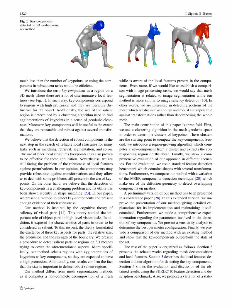
Fig. 1 Key-componentsdetected on 3D meshes usingour method

much less than the number of keypoints, so using the com-ponents in subsequent tasks would be efficient.

We introduce the term key-component as a region on a3D mesh where there are a lot of discriminative local fea-tures (see Fig. 1). In such way, key-components correspondto regions with high protrusion and they are therefore dis-tinctive for the object. Additionally, the size of the salientregion is determined by a clustering algorithm used to findagglomerations of keypoints in a sense of geodesic close-ness. Moreover, key-components will be useful to the extentthat they are repeatable and robust against several transfor-mations.

We believe that the detection of robust components is thenext step in the search of reliable local structures for manytasks such as matching, retrieval, segmentation, and so on.The use of finer local structures (keypoints) has also provento be effective for these application. Nevertheless, we arestill facing the problem of the robustness of local featuresagainst perturbations. In our opinion, the components mayprovide robustness against transformations and they allowus to deal with some problems still present in the use of key-points. On the other hand, we believe that the detection ofkey-components is a challenging problem and its utility hasbeen shown recently in shape matching [23]. In our paper,we present a method to detect key-components and presentenough evidence of their robustness.

Our method is inspired by the cognitive theory ofsaliency of visual parts [11]. This theory studied the im-portant role of object parts in high-level vision tasks. In ad-dition, it exposed the characteristics of parts in order to beconsidered as salient. To this respect, the theory formulatedthe existence of three key aspects for parts: the relative size,the protrusion and the strength of the boundary. We presenta procedure to detect salient parts or regions on 3D meshestrying to cover the aforementioned aspects. More specif-ically, our method selects regions with agglomerations ofkeypoints as key-components, so they are expected to havea high protrusion. Additionally, our results confirm the factthat the size is important to define robust salient regions.

Our method differs from mesh segmentation methodsas it computes a non-complete decomposition of a mesh

while is aware of the local features present in the compo-nents. Even more, if we would like to establish a compari-son with image processing tasks, we would say that meshsegmentation is related to image segmentation while ourmethod is more similar to image saliency detection [10]. Inother words, we are interested in detecting portions of themesh which are distinctive enough and robust and repeatableagainst transformations rather than decomposing the wholemesh.

The main contribution of this paper is three-fold. First,we use a clustering algorithm in the mesh geodesic spacein order to determine clusters of keypoints. These clustersare the starting point to compute the key-components. Sec-ond, we introduce a region-growing algorithm which com-putes a key-component from a cluster and extracts the cor-responding region on the mesh. Finally, we show a com-prehensive evaluation of our approach in different scenar-ios. For the evaluation, we use a standard feature detectionbenchmark which contains shapes with several transforma-tions. Furthermore, we compare our method with a variationof the MSER components detection technique [20] whichmake use of the diffusion geometry to detect overlappingcomponents on meshes.

A preliminary version of our method has been presentedin a conference paper [28]. In this extended version, we im-prove the presentation of our method, giving detailed ex-planations for its implementation and maintaining it self-contained. Furthermore, we made a comprehensive exper-imentation regarding the parameters involved in the detec-tion of key-components. We present a sensitivity analysis todetermine the best parameter configuration. Finally, we pro-vide a comparison of our method with an existing methodand show that the key-components outperform the state ofthe art.

The rest of the paper is organized as follows. Section 2presents the related works regarding mesh decompositionand local features. Section 3 describes the local features de-tection and our algorithm for detecting the key-components.Section 4 shows the evaluation and discussion of the ob-tained results using the SHREC’10 feature detection and de-scription benchmark. Also, we propose a variation of a state-

Key-components: detection of salient regions on 3D meshes 1321

of-the-art method in order to compare it with our method.Finally, Sect. 5 concludes the paper.

2 Related work

Mesh decomposition is an important analysis tool with ap-plications in computer vision and graphics. The idea is topartition a given mesh in components or regions which canbe used in applications. Although there are a lot of ap-proaches for mesh segmentation, we are interested in thosemethods driven by local features. For a comprehensive studyabout mesh segmentation techniques, we recommend thesurvey by Shamir [24].

One of the earliest techniques for feature-driven meshdecomposition was presented by Mortara et al. [22]. Thismethod decomposes a triangular mesh based on a charac-terization of a vertex using its local curvature. It analyzesthe evolution of the curve formed by the intersection of themesh with a set of spheres with increasing radii. The numberof connected components of the curve and the local proper-ties (curvature and length ratio) define a classification foreach vertex, which is used to group vertices with similarfeatures. Differently, Huang et al. [13] proposed to decom-pose a shape based on a modal analysis. Taking the eigen-decomposition of the Hessian of an energy function definedon the mesh, it is possible to define the set of typical de-formations of a mesh. Therefore, this method is able to esti-mate the parts that tend to be rigid and subsequently segmentthem.

Local features have also been used for mesh segmenta-tion. Agathos et al. [1] propose a mesh segmentation methodbased on points of interest. Given a mesh, the algorithmcomputes a protrusion function for each vertex, which is de-fined as the sum of geodesic distances to all vertex on themesh. Thus, a vertex is selected as point of interest if thevalue of its protrusion function is greater than the mean ofgeodesic distances between each pair of vertices. The pointsof interest are grouped in order to avoid regions with manypoints of interest. Each point of interest is used as seed forcomputing the mesh segments. Similarly, Katz et al. [14]computed a 3D embedding for a shape and subsequently,the convex hull of the embedding was calculated. The ver-tices of the convex hull were considered as keypoints, overwhich the method computed a set of core components.

Also, Gal and Cohen-Or [9] proposed to represent a 3Dobject as a set of salient geometric features. Their schemeentirely relies on curvature information over the shape’s sur-face. This method starts by computing the curvature on aset of sampled points. Next, points are sorted according totheir curvature values. The algorithm takes points with highcurvature and performs a grouping of neighbor points un-til a good quadratic fitting surface can be found that ap-

proximates better the neighborhood. Subsequently, a region-growing algorithm clusters the mesh by adding points to theinitial segments according to an empirical measure whichinvolves area, curvature and similarity. The final clusters arecalled salient geometric features which are used in shapematching.

On the other hand, Hu and Hua [12] proposed to findkeypoints using the eigen-decomposition of the Laplace–Beltrami operator of a shape. Each keypoint has a scalewhich is used to define a local patch, so a mesh is repre-sented as a set of local patches product of the keypoint-based decomposition. After describing each local patch withits Laplace–Beltrami spectrum, they are used in a matchingalgorithm. On the other hand, Toldo et al. [32] applied a seg-mentation based on local properties of the mesh, specificallya shape index computed from the principal curvature values.Each segment is described with a histogram of local proper-ties. Finally, a bag of features approach is used for describethe entire shape in order to be used in shape retrieval. Differ-ently, Shapira et al. [25] performed a hierarchical segmenta-tion using a shape diameter function (SDF). Subsequently,each segment is described using several local features suchas a normalized histogram of SDF, shape distribution sig-natures and conformal geometry signatures. The signatureswere used in matching and retrieval.

More recently, the decomposition of meshes from spec-tral functions defined on the surface has been introduced.The idea of these techniques is to take advantage of intrin-sic information to define a function on vertices, edges orfaces. Subsequently, the defined function is used by a group-ing algorithm which provides a segmentation. For instance,the Heat Mapping approach [8] defines a vertex signaturewhich can be interpreted as the average temperature on thesurface by applying heat on a vertex. Then, a segmentationprocess using the k-means algorithm is driven from pointswith the highest value of heat affinity. Similarly, the Center-Shift method [31] proposes the evaluation of the biharmonickernel in a point as a vertex function. Next, the algorithmfinds a set of termination points which are vertices with max-imal weighted mean of the defined function evaluated in lo-cal neighborhoods. Finally, a segment refinement is appliedto provide the final segmentation.

Likewise, Skraba et al. [29] proposed to assign to eachvertex its heat kernel signature evaluated in a fixed time.With these values, the technique applies a persistence-basedclustering. This clustering considers to track regions associ-ated with local maxima of the function. On the other hand,Aubry et al. [2] computed an n-dimensional function foreach vertex. Each vertex was represented by its wave ker-nel signature. Next, every descriptor from a training set ofshapes is collected in a large n-dimensional point cloud.This points are clustered by a Gaussian mixture algorithmwhere points in the same cluster correspond to the same


mesh segment. This clusters are used for assigning a labelto each vertex of a new shape.

In the same direction, the extension of methods from im-age processing and computer vision has been studied. For in-stance, Digne et al. [6] extend the maximally stable extremalregions (MSER) to shape decomposition. The method usedthe concept of vertex-weighted component trees applied tomeshes. To accomplish this goal, it was necessary to use themean curvature as function defined over the mesh. Similarly,Litman et al. [20] also used the MSER framework to detectstable components on meshes. The authors proposed an ap-proach based on diffusion geometry. The algorithm consid-ers the shape as a graph and associates weights to verticesand edges according to the evaluation of a local property(the heat kernel) between vertices and edges. A very inter-esting work that also uses concepts from image processing isthe Variational Mesh Decomposition [33]. It is based on thewell-studied Mumford–Shah functional which is commonin image segmentation literature. This technique proposes aconvex version of the functional which is applied on a face-based multichannel function on the surface. The function isdefined from the eigenvectors of a Laplacian matrix definedon dihedral angles for edges.

Saliency on meshes Previous approaches for detectingsaliency on 3D meshes are mainly focused on defining asaliency function on surface points [15, 17, 18, 26]. Never-theless, in these approaches, it is not clear the connectionbetween the point saliency and the determination of a re-gion with boundary. In addition, there is no robustness eval-uation of the proposed techniques against transformations.This is important in order to guarantee effectiveness in fur-ther processes and applications such as shape recognitionand retrieval. Our paper attempts to cover these two aspectsby presenting a technique that detects robust salient regionsand making an extensive evaluation.

3 Key-component detection

Our method consists of three steps: keypoint detection, clus-tering in the geodesic space, and key-component extraction.Our proposal is based on the detection of points of interest,which can be effectively used for detecting stable compo-nents on meshes. In the literature, there are many techniquesto detect keypoints, with different approaches and advan-tages. In this work, we use the Harris 3D method [27], whichhas proven to be effective and efficient in various scenar-ios. In order to maintain the paper self-contained, we beginour description with a brief introduction to the Harris 3Dmethod, and then we will describe how the keypoints areused to detect the mesh components.

3.1 Keypoints detection

Given a 3D mesh, we need to find points of interest on it.In general terms, an point of interest is a point on the meshsurface with a neighborhood geometrically unusual. For in-stance, many approaches link this definition with the cur-vature measured on the vertices of the mesh. So, points onnearly planar regions would not be considered as interesting.A keypoint detection method is robust if it works accordingwith the previous criterion. However, it also needs to be in-sensitive to noise, tessellations, and missing data (holes orrange data). The Harris 3D method is an extension of thewell-known operator in computer vision and it has provento be an alternative to cope with the aforementioned prob-lems.

Briefly, the idea is to represent the neighborhood around avertex as an oriented image patch, and subsequently to applythe Harris operator in an effective way. First, the algorithmtries to find an adaptive neighborhood around a vertex usingan algorithm robust to geometric changes. Second, the orien-tation of the local patch is found by applying PCA over thelocal neighborhood. This step converts the oriented imagepatch into a canonical representation invariant to orientation.Third, a quadratic surface is fitted to the transformed localpatch. Fourth, the method computes the smoothed deriva-tives of the fitted surface by convolving it with Gaussianfunctions. Fifth, using the derivatives, the Harris responseis calculated using an autocorrelation function. Finally, theresponses are used to determine the final set of points of in-terest selecting those vertices with the higher responses.

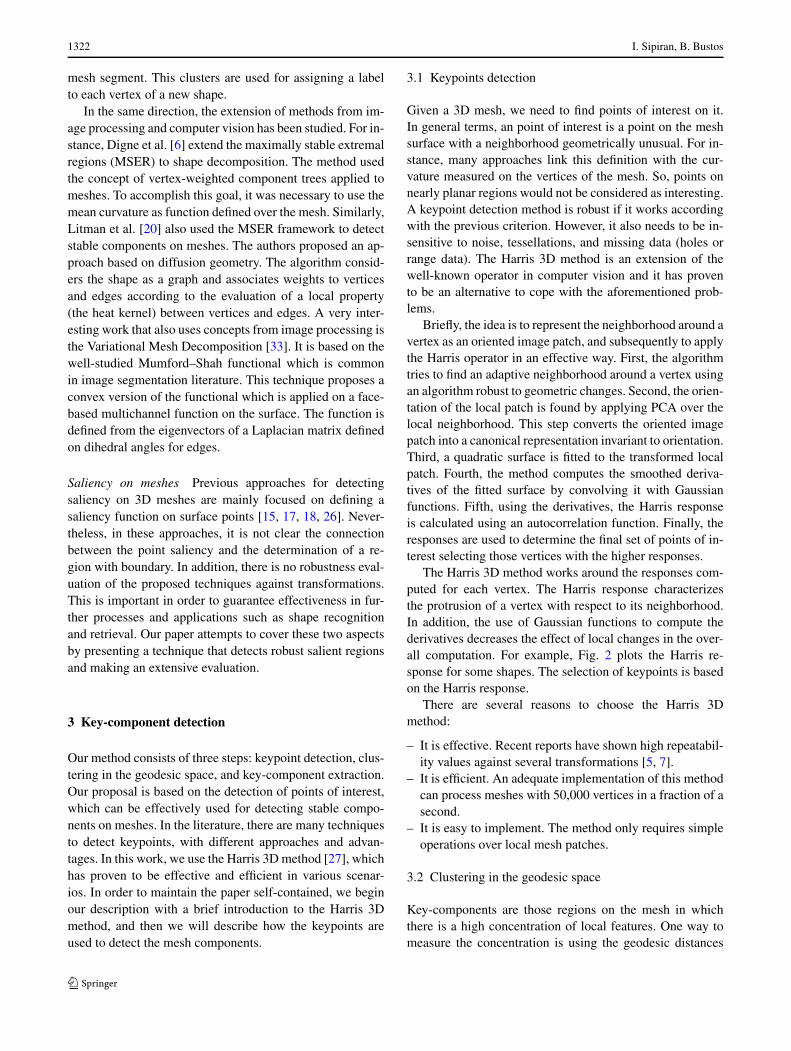
The Harris 3D method works around the responses com-puted for each vertex. The Harris response characterizesthe protrusion of a vertex with respect to its neighborhood.In addition, the use of Gaussian functions to compute thederivatives decreases the effect of local changes in the over-all computation. For example, Fig. 2 plots the Harris re-sponse for some shapes. The selection of keypoints is basedon the Harris response.

There are several reasons to choose the Harris 3Dmethod:

– It is effective. Recent reports have shown high repeatabil-ity values against several transformations [5, 7].

– It is efficient. An adequate implementation of this methodcan process meshes with 50,000 vertices in a fraction of asecond.

– It is easy to implement. The method only requires simpleoperations over local mesh patches.

3.2 Clustering in the geodesic space

Key-components are those regions on the mesh in whichthere is a high concentration of local features. One way tomeasure the concentration is using the geodesic distances


Fig. 2 Harris 3D operator plotted as a saliency value for each vertex. Note how the high values are present in discriminative regions of the meshes

between the keypoints, and therefore grouping them accord-ing to their closeness in terms of this kind of distance. LetS = {s1, s2, . . . , sn} be the set of keypoints previously de-tected, our goal is to find partitions Si ⊂ S, i = 1, . . . ,m

over the set of keypoints S in order to fulfill the followingproperties:

1. dgeod(x, y) ≤ R, ∀x, y ∈ Si .2. dgeod(x, y) ≥ T , ∀x ∈ Si and ∀y ∈ Sj , i �= j .3. |Si | ≥ N,∀i.4.

⋃mi=1 Si ⊆ S.

Property 1 suggests that elements in a subset Si shareapproximately the same location on the mesh (threshold R

controls the proximity permitted). Property 2 states that twosubsets Si and Sj cannot be very close to each other (thresh-old T controls how far two subset should be). Property 3establishes that each partition should contain a minimumnumber of keypoints to be considered as a valid partition.Property 4 considers a non-complete partitioning of the ini-tial set S. Obviously, there may be keypoints which meetthe two first properties, but not the third. This is becausesome points of interest could be isolated, and therefore theywould not belong to any partition. Moreover, isolated key-points could have been selected due to noise. It is clear that,in order to detect consistent components on meshes, we needto discard isolated keypoints. Finally, property 5 defines adisjoint partition of the set S.

In practice, we need to consider a clustering process re-garding the geodesic distances between keypoints. In orderto accomplish this goal, our method computes a set P ∈R

2,in which Euclidean distances between elements in P ap-proximately preserve the geodesic distances between ele-ments in S. That is, we need to find the set P such that

P = argminp1,...,pn

∑

i<j

(‖pi − pj‖ − dgeod(si , sj ))

(1)

where each pi ∈R2 corresponds to the keypoint si ∈ S.

This problem is commonly called MultidimensionalScaling [3] and it is used to embed points in one space into

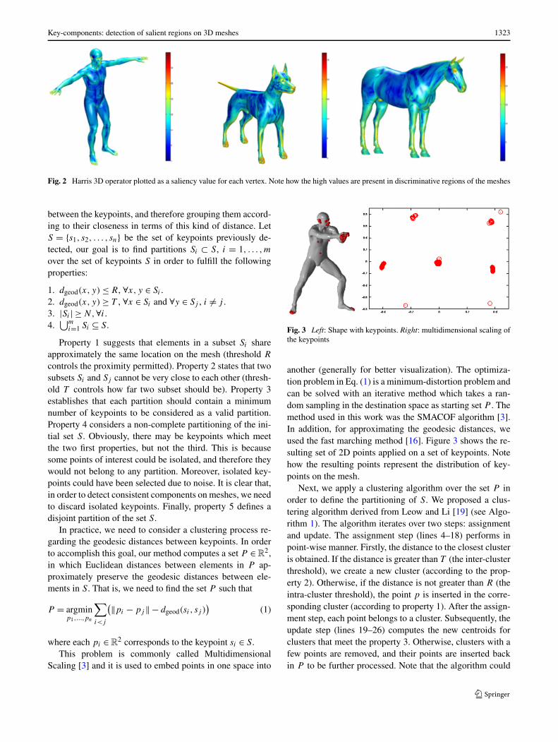
Fig. 3 Left: Shape with keypoints. Right: multidimensional scaling ofthe keypoints

another (generally for better visualization). The optimiza-tion problem in Eq. (1) is a minimum-distortion problem andcan be solved with an iterative method which takes a ran-dom sampling in the destination space as starting set P . Themethod used in this work was the SMACOF algorithm [3].In addition, for approximating the geodesic distances, weused the fast marching method [16]. Figure 3 shows the re-sulting set of 2D points applied on a set of keypoints. Notehow the resulting points represent the distribution of key-points on the mesh.

Next, we apply a clustering algorithm over the set P inorder to define the partitioning of S. We proposed a clus-tering algorithm derived from Leow and Li [19] (see Algo-rithm 1). The algorithm iterates over two steps: assignmentand update. The assignment step (lines 4–18) performs inpoint-wise manner. Firstly, the distance to the closest clusteris obtained. If the distance is greater than T (the inter-clusterthreshold), we create a new cluster (according to the prop-erty 2). Otherwise, if the distance is not greater than R (theintra-cluster threshold), the point p is inserted in the corre-sponding cluster (according to property 1). After the assign-ment step, each point belongs to a cluster. Subsequently, theupdate step (lines 19–26) computes the new centroids forclusters that meet the property 3. Otherwise, clusters with afew points are removed, and their points are inserted backin P to be further processed. Note that the algorithm could


Algorithm 1 Adaptive clusteringRequire: Set of points P

Require: Inter-cluster distance T

Require: Intra-cluster distance R

Require: Minimum number of elements per cluster N

Require: Number of iterations IterEnsure: Set of clusters C = {C1, . . . ,Cm}

1: Let C a set of clusters2: C ← ∅3: for j ← 1 to Iter do4: for each p ∈ P do5: if C = ∅ then6: d = 2T

7: else8: C∗ = arg minCi∈Cdist(p,Ci)

9: d = distance from p to C∗10: end if11: if d > T then12: Cnew = {p}13: C ← C ∪ Cnew

14: P ← P − {p}15: else if d ≤ R then16: C∗ ← C∗ ∪ {p}17: P ← P − {p}18: end if19: end for20: for i ← 1 to |C| do21: if |C∗| ≥ N then22: Update centroid for C∗23: else24: P ← P ∪ C∗25: C ← C\{C∗}26: end if27: end for28: end for29: Return C

converge before the last iteration, however, we opt for usinga number of iterations as stop criterion. In all experimentspresented in Sect. 4, we set Iter = 10. This value was setempirically from the observation that, on average, the clus-tering algorithm converges in 6–8 iterations.

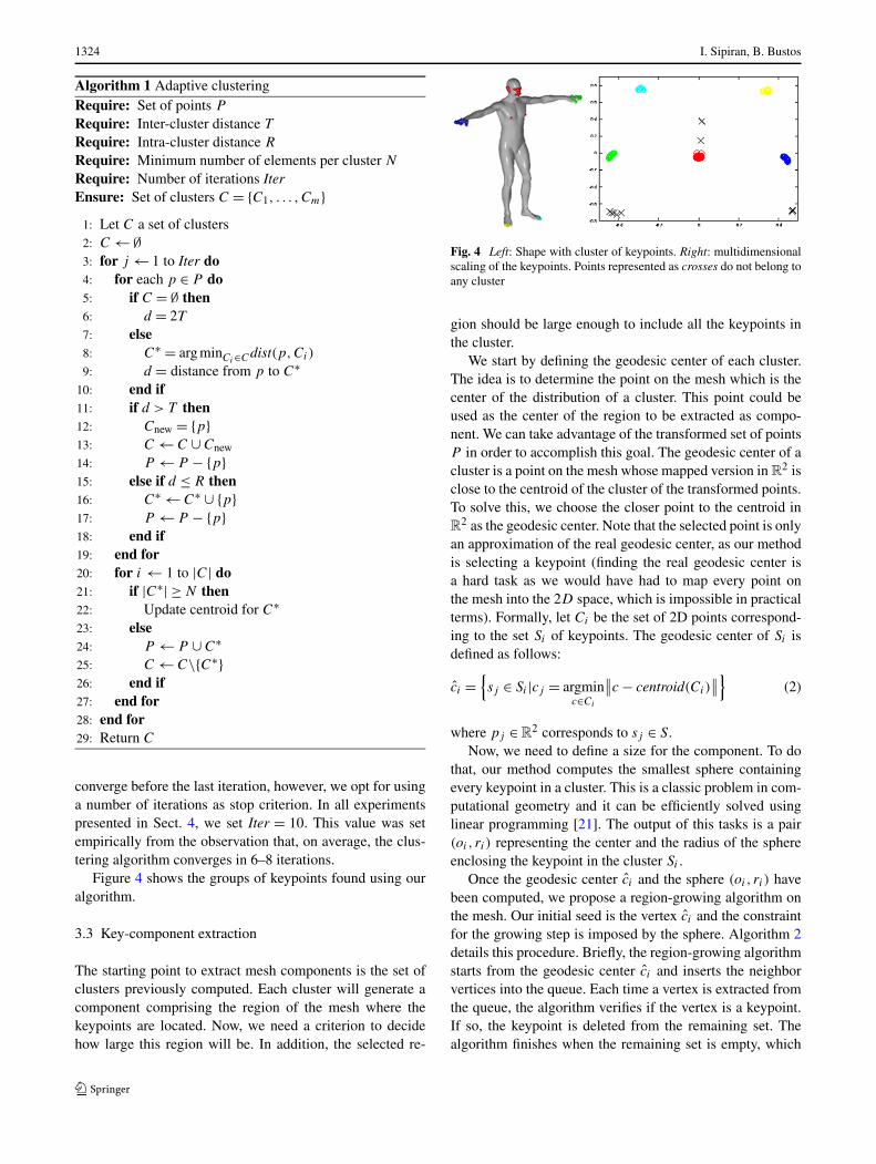
Figure 4 shows the groups of keypoints found using ouralgorithm.

3.3 Key-component extraction

The starting point to extract mesh components is the set ofclusters previously computed. Each cluster will generate acomponent comprising the region of the mesh where thekeypoints are located. Now, we need a criterion to decidehow large this region will be. In addition, the selected re-

Fig. 4 Left: Shape with cluster of keypoints. Right: multidimensionalscaling of the keypoints. Points represented as crosses do not belong toany cluster

gion should be large enough to include all the keypoints inthe cluster.

We start by defining the geodesic center of each cluster.The idea is to determine the point on the mesh which is thecenter of the distribution of a cluster. This point could beused as the center of the region to be extracted as compo-nent. We can take advantage of the transformed set of pointsP in order to accomplish this goal. The geodesic center of acluster is a point on the mesh whose mapped version in R

2 isclose to the centroid of the cluster of the transformed points.To solve this, we choose the closer point to the centroid inR

2 as the geodesic center. Note that the selected point is onlyan approximation of the real geodesic center, as our methodis selecting a keypoint (finding the real geodesic center isa hard task as we would have had to map every point onthe mesh into the 2D space, which is impossible in practicalterms). Formally, let Ci be the set of 2D points correspond-ing to the set Si of keypoints. The geodesic center of Si isdefined as follows:

ci ={sj ∈ Si |cj = argmin

c∈Ci

∥∥c − centroid(Ci)

∥∥}

(2)

where pj ∈R2 corresponds to sj ∈ S.

Now, we need to define a size for the component. To dothat, our method computes the smallest sphere containingevery keypoint in a cluster. This is a classic problem in com-putational geometry and it can be efficiently solved usinglinear programming [21]. The output of this tasks is a pair(oi, ri) representing the center and the radius of the sphereenclosing the keypoint in the cluster Si .

Once the geodesic center ci and the sphere (oi, ri) havebeen computed, we propose a region-growing algorithm onthe mesh. Our initial seed is the vertex ci and the constraintfor the growing step is imposed by the sphere. Algorithm 2details this procedure. Briefly, the region-growing algorithmstarts from the geodesic center ci and inserts the neighborvertices into the queue. Each time a vertex is extracted fromthe queue, the algorithm verifies if the vertex is a keypoint.If so, the keypoint is deleted from the remaining set. Thealgorithm finishes when the remaining set is empty, which


Fig. 5 Key-components detected on shapes with several transformations. From left to right: null shape, isometry, microholes, local scale, noise,topology, holes, sampling, and shot noise. Color are arbitrary

means that a component has been extracted and it containsthe complete set of input keypoints.

It is worth noting that we introduce a scaling factor σ > 1for the radius ri (Algorithm 2, line 15). Thus, we ensure aconnectivity between the keypoints in Si . A value greaterthan 1 would guarantee to find a connected component lyinginside the sphere with radius σ ×ri . That is, a suitable choicefor σ should be in the interval (1,2]. We avoid a value of onein our choice because the patch containing the cluster of key-points could contain more than one connected component.Indeed, the larger the σ value, the higher the probability thatthe extracted region is a connected component. On the otherhand, the σ value cannot be extremely large because it couldaffect the characterization of the cluster of keypoints. In allour experiments, we use σ = 1.5 which allow us to alwaysobtain one connected component in the extraction withoutcompromising the characterization of the keypoint clusters.

Figure 5 shows the components detected in severalshapes.

4 Experiments and results

In this section, we describe the dataset, the evaluation crite-rion used to assess our method, and the experimental results.

4.1 Dataset

In order to evaluate the proposed method, we used theSHREC’10 feature detection and description benchmark [5].This dataset is composed by three shapes (null shapes) anda set of shapes obtained by applying a set of transforma-tions on the null shapes. Shapes have approximately 10,000to 50,000 vertices and they were represented as triangu-lar meshes. The set of transformations applied on the nullshapes are isometry, micro-holes and big holes, topology,noise and shot noise, global and local scale, and downsam-pling. Each transformation was applied in five levels, so thetotal number of shapes in the dataset is 138.

In addition to the shapes, the dataset contains a groundtruth specifying the vertex-to-vertex correspondences be-tween the transformed and the null shapes. Also, the modelswere normalized so the surface area is 1. This facilitated theconfiguration of the parameters of clustering.

Algorithm 2 Key-component extractionRequire: Vertex set V

Require: Geodesic center ci

Require: Cluster of keypoints Si

Require: Sphere (oi, ri)

Require: Scaling radius factor σ

Ensure: Vertex set VR

Ensure: Face set FR

1: Let VR be an empty vertex set2: Let FR be an empty face set3: Let waiting be the set of remaining keypoints4: Let visited be a vertex queue5: visited.enqueue(ci)

6: waiting ← Si

7: while waiting �= ∅ and visited �= ∅ do8: v ← visited.dequeue()9: if v is not marked then

10: VR ← VR ∪ {v}11: Mark v

12: waiting ← waiting − {v}13: for each w ∈ v.adjacentVertices() do14: if w is not marked then15: if ‖w − oi‖ < σ × ri then16: visited.enqueue(w)

17: end if18: end if19: end for20: FR ← FR ∪ v.adjacentFaces()21: end if22: end while23: Unmark vertices24: Return FV and FR

4.2 Evaluation criterion

To evaluate our approach, we use the methodology previ-ously used in Litman et al. [20] to determine the repeata-bility of a decomposition. Our goal is to determine if themesh components are consistent between a null shape and atransformed shape. Given a null shape X and a transformedmesh Y , the components are represented as X1, . . . ,Xn and


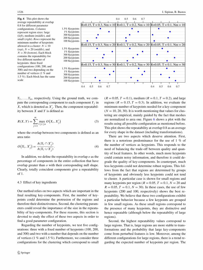
Fig. 6 This plot shows theaverage repeatability at overlap0.8 for different parameterconfigurations. Columnsrepresent region sizes: large(left), medium (middle), andsmall (right). Rows represent theminimum number of keypointsallowed in a cluster: N = 10(top), N = 20 (middle), andN = 30 (bottom). Each blockcontains the repeatability forfive different number ofkeypoints: three fixedconfigurations (100, 200, and300) and two depending on thenumber of vertices (1 % and1.5 %). Each block has the samescale

Y1, . . . , Ym, respectively. Using the ground truth, we com-pute the corresponding component to each component Yj inX, which is denoted as X′

j . Then, the component repeatabil-ity between X and Y is defined as

R(X,Y ) =m∑

j=1

max1≤i≤n

O(Xi,X

′j

)(3)

where the overlap between two components is defined as anarea ratio

O(Xi,X

′j

) = A(Xi ∩ X′j )

A(Xi ∪ X′j )

. (4)

In addition, we define the repeatability in overlap o as thepercentage of components in the entire collection that haveoverlap greater than o with their corresponding null shape.Clearly, totally coincident components give a repeatabilityof 1.

4.3 Effect of key ingredients

Our method relies on two aspects which are important in thefinal resulting key-components. First, the number of key-points could determine the protrusion of the regions andtherefore their distinctiveness. Second, the clustering param-eters could reveal the importance of the size in the repeata-bility of key-components. For these reasons, this section isdevoted to study the effect of these two aspects in order tofind a good parameter configuration.

Regarding the number of keypoints, we test five config-urations: three with a fixed number of keypoints (100, 200,and 300) and two with a number that depends on the numberof vertices (1 % and 1.5 %). Furthermore, we consider threeconfigurations for the clustering which correspond to small

(R = 0.05, T = 0.1), medium (R = 0.1, T = 0.2), and largeregions (R = 0.15, T = 0.3). In addition, we evaluate theminimum number of keypoints needed for a key-component(N = 10,20,30). It is worth mentioning that values for clus-tering are empirical, mainly guided by the fact that meshesare normalized to area one. Figure 6 shows a plot with theresults using all possible configuration as mentioned before.This plot shows the repeatability at overlap 0.8 as an averagefor every shape in the dataset (including transformations).

There are two aspects which deserve attention. First,there is a notorious predominance for the use of 1 % ofthe number of vertices as keypoints. This responds to theneed of balancing the trade-off between quality and quan-tity of local features. In other words, much more keypointscould contain noisy information, and therefore it could de-grade the quality of key-components. In counterpart, muchless keypoints could not determine robust regions. This fol-lows from the fact that regions are determined by groupsof keypoints and obviously less keypoints could not tendto cluster. A particular case is shown for small regions andmany keypoints per region (R = 0.05, T = 0.1,N = 20 andR = 0.05, T = 0.1,N = 30). In these cases, the use of fewkeypoints (200 and 100, respectively) shows the best re-peatability. We believe that these two configurations exhibita particular behavior because a few keypoints are groupedin few small regions. As these small regions correspond tothe presence of many keypoints, they are distinctive andhence repeatable (although below the repeatability of largeregions).

Second, the highest repeatability values correspond tolarge regions. That is, large regions are more stable to trans-formations and the probability that large key-componentscome from perturbed features is low. Moreover, among thedifferent configurations for large regions, there is a trend re-garding the expected number of keypoints per region. The


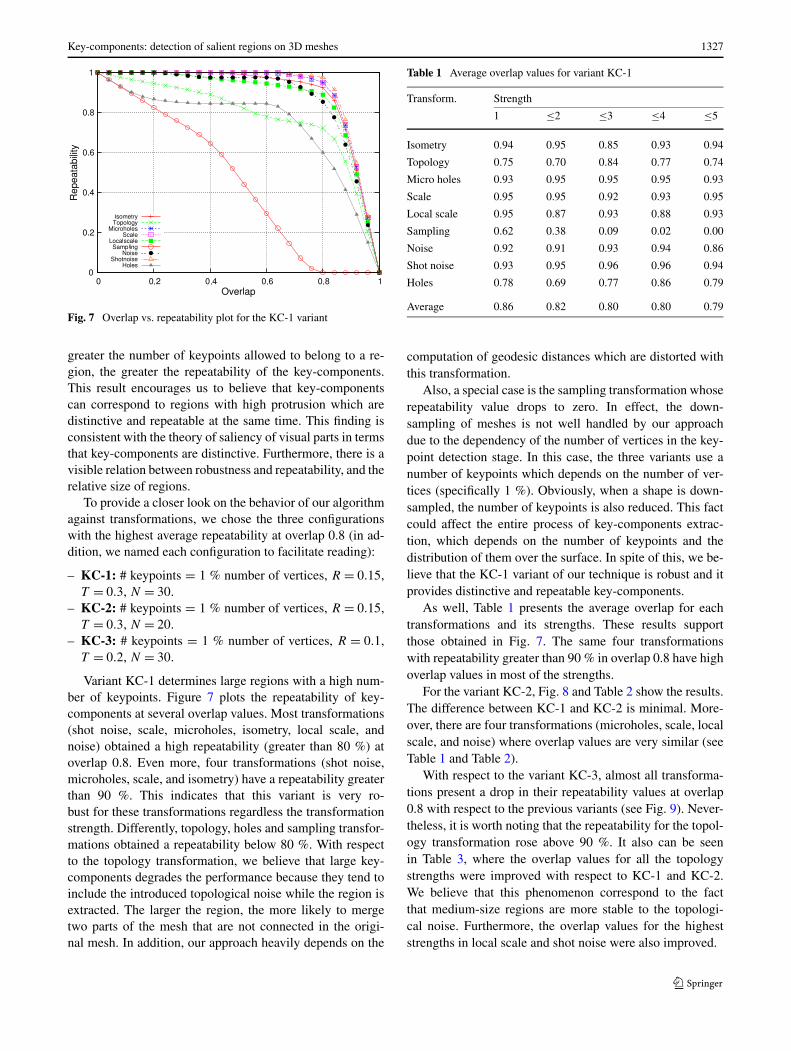
Fig. 7 Overlap vs. repeatability plot for the KC-1 variant

greater the number of keypoints allowed to belong to a re-gion, the greater the repeatability of the key-components.This result encourages us to believe that key-componentscan correspond to regions with high protrusion which aredistinctive and repeatable at the same time. This finding isconsistent with the theory of saliency of visual parts in termsthat key-components are distinctive. Furthermore, there is avisible relation between robustness and repeatability, and therelative size of regions.

To provide a closer look on the behavior of our algorithmagainst transformations, we chose the three configurationswith the highest average repeatability at overlap 0.8 (in ad-dition, we named each configuration to facilitate reading):

– KC-1: # keypoints = 1 % number of vertices, R = 0.15,T = 0.3, N = 30.



Variant KC-1 determines large regions with a high num-ber of keypoints. Figure 7 plots the repeatability of key-components at several overlap values. Most transformations(shot noise, scale, microholes, isometry, local scale, andnoise) obtained a high repeatability (greater than 80 %) atoverlap 0.8. Even more, four transformations (shot noise,microholes, scale, and isometry) have a repeatability greaterthan 90 %. This indicates that this variant is very ro-bust for these transformations regardless the transformationstrength. Differently, topology, holes and sampling transfor-mations obtained a repeatability below 80 %. With respectto the topology transformation, we believe that large key-components degrades the performance because they tend toinclude the introduced topological noise while the region isextracted. The larger the region, the more likely to mergetwo parts of the mesh that are not connected in the origi-nal mesh. In addition, our approach heavily depends on the

Table 1 Average overlap values for variant KC-1

Transform. Strength

1 ≤2 ≤3 ≤4 ≤5

Isometry 0.94 0.95 0.85 0.93 0.94

Topology 0.75 0.70 0.84 0.77 0.74

Micro holes 0.93 0.95 0.95 0.95 0.93

Scale 0.95 0.95 0.92 0.93 0.95

Local scale 0.95 0.87 0.93 0.88 0.93

Sampling 0.62 0.38 0.09 0.02 0.00

Noise 0.92 0.91 0.93 0.94 0.86

Shot noise 0.93 0.95 0.96 0.96 0.94

Holes 0.78 0.69 0.77 0.86 0.79

Average 0.86 0.82 0.80 0.80 0.79

computation of geodesic distances which are distorted withthis transformation.

Also, a special case is the sampling transformation whoserepeatability value drops to zero. In effect, the down-sampling of meshes is not well handled by our approachdue to the dependency of the number of vertices in the key-point detection stage. In this case, the three variants use anumber of keypoints which depends on the number of ver-tices (specifically 1 %). Obviously, when a shape is down-sampled, the number of keypoints is also reduced. This factcould affect the entire process of key-components extrac-tion, which depends on the number of keypoints and thedistribution of them over the surface. In spite of this, we be-lieve that the KC-1 variant of our technique is robust and itprovides distinctive and repeatable key-components.

As well, Table 1 presents the average overlap for eachtransformations and its strengths. These results supportthose obtained in Fig. 7. The same four transformationswith repeatability greater than 90 % in overlap 0.8 have highoverlap values in most of the strengths.

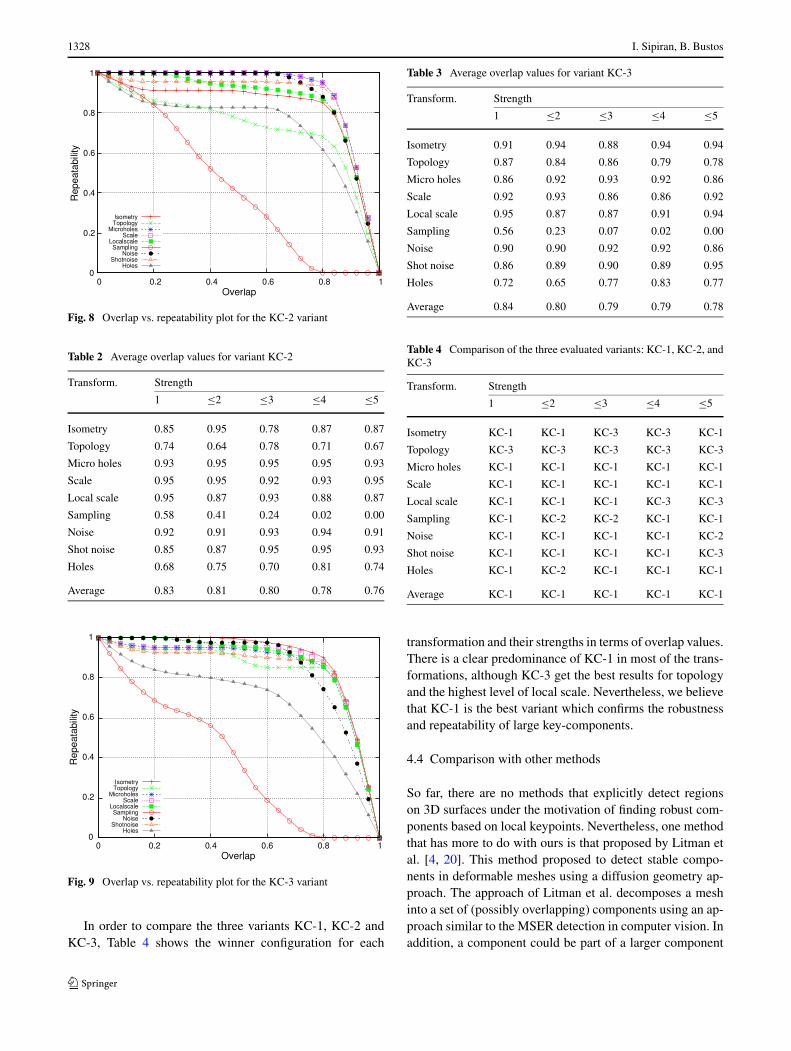
For the variant KC-2, Fig. 8 and Table 2 show the results.The difference between KC-1 and KC-2 is minimal. More-over, there are four transformations (microholes, scale, localscale, and noise) where overlap values are very similar (seeTable 1 and Table 2).

With respect to the variant KC-3, almost all transforma-tions present a drop in their repeatability values at overlap0.8 with respect to the previous variants (see Fig. 9). Never-theless, it is worth noting that the repeatability for the topol-ogy transformation rose above 90 %. It also can be seenin Table 3, where the overlap values for all the topologystrengths were improved with respect to KC-1 and KC-2.We believe that this phenomenon correspond to the factthat medium-size regions are more stable to the topologi-cal noise. Furthermore, the overlap values for the higheststrengths in local scale and shot noise were also improved.




Transform. Strength

1 ≤2 ≤3 ≤4 ≤5

Isometry 0.85 0.95 0.78 0.87 0.87

Topology 0.74 0.64 0.78 0.71 0.67

Micro holes 0.93 0.95 0.95 0.95 0.93

Scale 0.95 0.95 0.92 0.93 0.95

Local scale 0.95 0.87 0.93 0.88 0.87

Sampling 0.58 0.41 0.24 0.02 0.00

Noise 0.92 0.91 0.93 0.94 0.91

Shot noise 0.85 0.87 0.95 0.95 0.93

Holes 0.68 0.75 0.70 0.81 0.74

Average 0.83 0.81 0.80 0.78 0.76


In order to compare the three variants KC-1, KC-2 andKC-3, Table 4 shows the winner configuration for each


Transform. Strength

1 ≤2 ≤3 ≤4 ≤5

Isometry 0.91 0.94 0.88 0.94 0.94

Topology 0.87 0.84 0.86 0.79 0.78

Micro holes 0.86 0.92 0.93 0.92 0.86

Scale 0.92 0.93 0.86 0.86 0.92

Local scale 0.95 0.87 0.87 0.91 0.94

Sampling 0.56 0.23 0.07 0.02 0.00

Noise 0.90 0.90 0.92 0.92 0.86

Shot noise 0.86 0.89 0.90 0.89 0.95

Holes 0.72 0.65 0.77 0.83 0.77

Average 0.84 0.80 0.79 0.79 0.78

Table 4 Comparison of the three evaluated variants: KC-1, KC-2, andKC-3

Transform. Strength

1 ≤2 ≤3 ≤4 ≤5

Isometry KC-1 KC-1 KC-3 KC-3 KC-1

Topology KC-3 KC-3 KC-3 KC-3 KC-3

Micro holes KC-1 KC-1 KC-1 KC-1 KC-1

Scale KC-1 KC-1 KC-1 KC-1 KC-1

Local scale KC-1 KC-1 KC-1 KC-3 KC-3

Sampling KC-1 KC-2 KC-2 KC-1 KC-1

Noise KC-1 KC-1 KC-1 KC-1 KC-2

Shot noise KC-1 KC-1 KC-1 KC-1 KC-3

Holes KC-1 KC-2 KC-1 KC-1 KC-1

Average KC-1 KC-1 KC-1 KC-1 KC-1

transformation and their strengths in terms of overlap values.There is a clear predominance of KC-1 in most of the trans-formations, although KC-3 get the best results for topologyand the highest level of local scale. Nevertheless, we believethat KC-1 is the best variant which confirms the robustnessand repeatability of large key-components.

4.4 Comparison with other methods

So far, there are no methods that explicitly detect regionson 3D surfaces under the motivation of finding robust com-ponents based on local keypoints. Nevertheless, one methodthat has more to do with ours is that proposed by Litman etal. [4, 20]. This method proposed to detect stable compo-nents in deformable meshes using a diffusion geometry ap-proach. The approach of Litman et al. decomposes a meshinto a set of (possibly overlapping) components using an ap-proach similar to the MSER detection in computer vision. Inaddition, a component could be part of a larger component


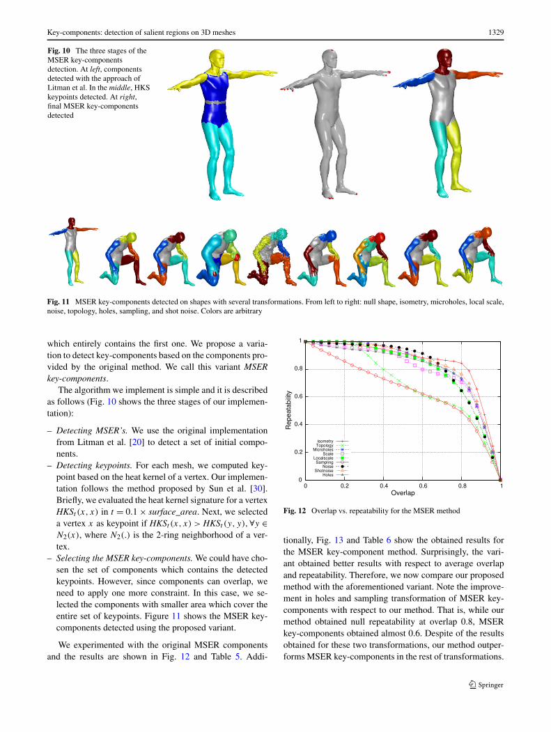
Fig. 10 The three stages of theMSER key-componentsdetection. At left, componentsdetected with the approach ofLitman et al. In the middle, HKSkeypoints detected. At right,final MSER key-componentsdetected

Fig. 11 MSER key-components detected on shapes with several transformations. From left to right: null shape, isometry, microholes, local scale,noise, topology, holes, sampling, and shot noise. Colors are arbitrary

which entirely contains the first one. We propose a varia-tion to detect key-components based on the components pro-vided by the original method. We call this variant MSERkey-components.

The algorithm we implement is simple and it is describedas follows (Fig. 10 shows the three stages of our implemen-tation):

– Detecting MSER’s. We use the original implementationfrom Litman et al. [20] to detect a set of initial compo-nents.

– Detecting keypoints. For each mesh, we computed key-point based on the heat kernel of a vertex. Our implemen-tation follows the method proposed by Sun et al. [30].Briefly, we evaluated the heat kernel signature for a vertexHKSt (x, x) in t = 0.1 × surface_area. Next, we selecteda vertex x as keypoint if HKSt (x, x) > HKSt (y, y),∀y ∈N2(x), where N2(.) is the 2-ring neighborhood of a ver-tex.

– Selecting the MSER key-components. We could have cho-sen the set of components which contains the detectedkeypoints. However, since components can overlap, weneed to apply one more constraint. In this case, we se-lected the components with smaller area which cover theentire set of keypoints. Figure 11 shows the MSER key-components detected using the proposed variant.

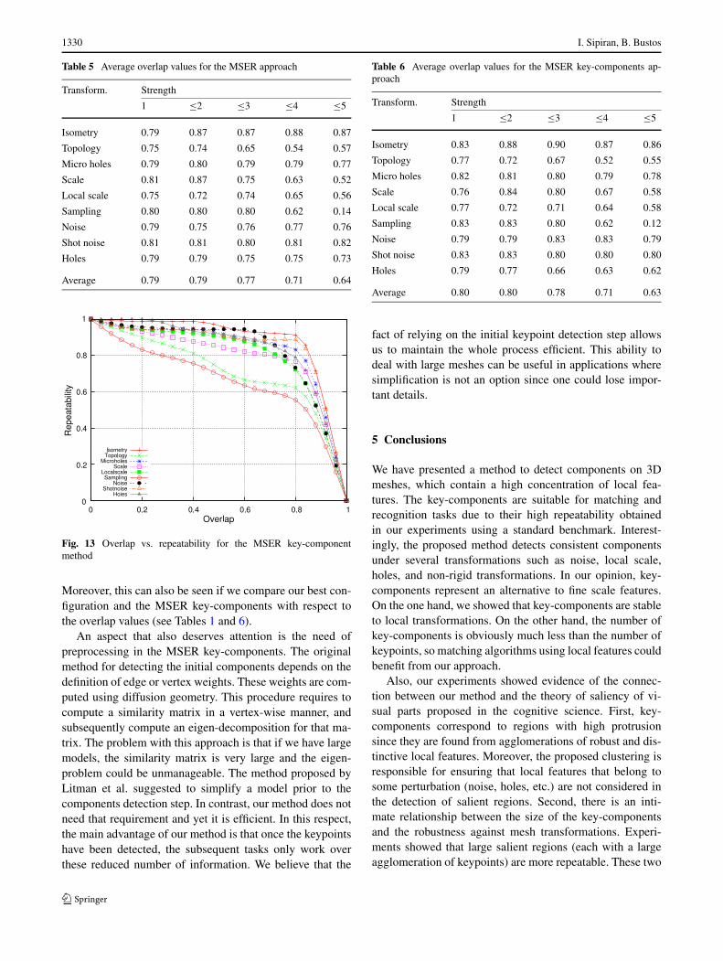
We experimented with the original MSER componentsand the results are shown in Fig. 12 and Table 5. Addi-

Fig. 12 Overlap vs. repeatability for the MSER method

tionally, Fig. 13 and Table 6 show the obtained results forthe MSER key-component method. Surprisingly, the vari-ant obtained better results with respect to average overlapand repeatability. Therefore, we now compare our proposedmethod with the aforementioned variant. Note the improve-ment in holes and sampling transformation of MSER key-components with respect to our method. That is, while ourmethod obtained null repeatability at overlap 0.8, MSERkey-components obtained almost 0.6. Despite of the resultsobtained for these two transformations, our method outper-forms MSER key-components in the rest of transformations.


Table 5 Average overlap values for the MSER approach

Transform. Strength

1 ≤2 ≤3 ≤4 ≤5

Isometry 0.79 0.87 0.87 0.88 0.87

Topology 0.75 0.74 0.65 0.54 0.57

Micro holes 0.79 0.80 0.79 0.79 0.77

Scale 0.81 0.87 0.75 0.63 0.52

Local scale 0.75 0.72 0.74 0.65 0.56

Sampling 0.80 0.80 0.80 0.62 0.14

Noise 0.79 0.75 0.76 0.77 0.76

Shot noise 0.81 0.81 0.80 0.81 0.82

Holes 0.79 0.79 0.75 0.75 0.73

Average 0.79 0.79 0.77 0.71 0.64

Fig. 13 Overlap vs. repeatability for the MSER key-componentmethod

Moreover, this can also be seen if we compare our best con-figuration and the MSER key-components with respect tothe overlap values (see Tables 1 and 6).

An aspect that also deserves attention is the need ofpreprocessing in the MSER key-components. The originalmethod for detecting the initial components depends on thedefinition of edge or vertex weights. These weights are com-puted using diffusion geometry. This procedure requires tocompute a similarity matrix in a vertex-wise manner, andsubsequently compute an eigen-decomposition for that ma-trix. The problem with this approach is that if we have largemodels, the similarity matrix is very large and the eigen-problem could be unmanageable. The method proposed byLitman et al. suggested to simplify a model prior to thecomponents detection step. In contrast, our method does notneed that requirement and yet it is efficient. In this respect,the main advantage of our method is that once the keypointshave been detected, the subsequent tasks only work overthese reduced number of information. We believe that the

Table 6 Average overlap values for the MSER key-components ap-proach

Transform. Strength

1 ≤2 ≤3 ≤4 ≤5

Isometry 0.83 0.88 0.90 0.87 0.86

Topology 0.77 0.72 0.67 0.52 0.55

Micro holes 0.82 0.81 0.80 0.79 0.78

Scale 0.76 0.84 0.80 0.67 0.58

Local scale 0.77 0.72 0.71 0.64 0.58

Sampling 0.83 0.83 0.80 0.62 0.12

Noise 0.79 0.79 0.83 0.83 0.79

Shot noise 0.83 0.83 0.80 0.80 0.80

Holes 0.79 0.77 0.66 0.63 0.62

Average 0.80 0.80 0.78 0.71 0.63

fact of relying on the initial keypoint detection step allowsus to maintain the whole process efficient. This ability todeal with large meshes can be useful in applications wheresimplification is not an option since one could lose impor-tant details.

5 Conclusions

We have presented a method to detect components on 3Dmeshes, which contain a high concentration of local fea-tures. The key-components are suitable for matching andrecognition tasks due to their high repeatability obtainedin our experiments using a standard benchmark. Interest-ingly, the proposed method detects consistent componentsunder several transformations such as noise, local scale,holes, and non-rigid transformations. In our opinion, key-components represent an alternative to fine scale features.On the one hand, we showed that key-components are stableto local transformations. On the other hand, the number ofkey-components is obviously much less than the number ofkeypoints, so matching algorithms using local features couldbenefit from our approach.

Also, our experiments showed evidence of the connec-tion between our method and the theory of saliency of vi-sual parts proposed in the cognitive science. First, key-components correspond to regions with high protrusionsince they are found from agglomerations of robust and dis-tinctive local features. Moreover, the proposed clustering isresponsible for ensuring that local features that belong tosome perturbation (noise, holes, etc.) are not considered inthe detection of salient regions. Second, there is an inti-mate relationship between the size of the key-componentsand the robustness against mesh transformations. Experi-ments showed that large salient regions (each with a largeagglomeration of keypoints) are more repeatable. These two


aspects are consistent with the aforementioned theory, so ourmethod can be thought of as a method embodying this the-ory.

Acknowledgements This project has been partially funded by CON-ICYT (Chile) through the Doctoral Scholarship, and FONDECYT(Chile) Project 1110111. We would like to thank Roee Litman for gen-tly providing us the implementation of MSER components for our eval-uation. Also, we thank Michael Bronstein for his extremely useful helpwith the SHREC’2010 feature detection and description benchmark.

References

1. Agathos, A., Pratikakis, I., Perantonis, S., Sapidis, N.S.:Protrusion-oriented 3D mesh segmentation. Vis. Comput. 26(1),63–81 (2009)

2. Aubry, M., Schlickewei, U., Cremers, D.: Pose-consistent 3Dshape segmentation based on a quantum mechanical feature de-scriptor. In: Mester, R., Felsberg, M. (eds.) DAGM-Symposium.Lecture Notes in Computer Science, vol. 6835, pp. 122–131.Springer, Berlin (2011)

3. Borg, I., Groenen, P.: Modern Multidimensional Scaling: Theoryand Applications. Springer, Berlin (2005)

4. Boyer, E., Bronstein, A., Bronstein, M., Bustos, B., Darom, T.,Horaud, R., Hotz, I., Keller, Y., Keustermans, J., Kovnatsky, A.,Litman, R., Reininghaus, J., Sipiran, I., Smeets, D., Suetens, P.,Vandermeulen, D., Zaharescu, A., Zobel, V.: SHREC 2011: robustfeature detection and description benchmark. In: Proc. Eurograph-ics 2011 Workshop on 3D Object Retrieval (3DOR’11), pp. 71–78.Eurographics Association, Aire-la-Ville (2011)

5. Bronstein, A.M., Bronstein, M.M., Bustos, B., Castellani, U.,Crisani, M., Falcidieno, B., Guibas, L.J., Kokkinos, I., Murino,V., Sipiran, I., Ovsjanikov, M., Patanè, G., Spagnuolo, M., Sun,J.: SHREC 2010: robust feature detection and description bench-mark. In: Proc. Workshop on 3D Object Retrieval (3DOR’10), Eu-rographics Association, Aire-la-Ville (2010)

6. Digne, J., Morel, J.M., Audfray, N., Mehdi-Souzani, C.: The levelset tree on meshes. In: Proc. of the Fifth Int. Symposium on 3DData Processing, Visualization and Transmission, Paris, France(2010)

7. Dutagaci, H., Cheung, C., Godil, A.: Evaluation of 3D interestpoint detection techniques via human-generated ground truth. Vis.Comput. 28, 901–917 (2012)

8. Fang, Y., Sun, M., Kim, M., Ramani, K.: Heat-mapping: a robustapproach toward perceptually consistent mesh segmentation. In:IEEE Computer Vision and Pattern Recognition, pp. 2145–2152(2011)

9. Gal, R., Cohen-Or, D.: Salient geometric features for partial shapematching and similarity. ACM Trans. Graph. 25(1), 130–150(2006)

10. Goferman, S., Zelnik-Manor, L., Tal, A.: Context-aware saliencydetection. IEEE Trans. Pattern Anal. Mach. Intell. 34(10), 1915–1926 (2012)

11. Hoffman, D.D., Singh, M.: Salience of visual parts. Cognition63(1), 29–78 (1997)

12. Hu, J., Hua, J.: Salient spectral geometric features for shapematching and retrieval. Vis. Comput. 25(5–7), 667–675 (2009)

13. Huang, Q.X., Wicke, M., Adams, B., Guibas, L.: Shape decompo-sition using modal analysis. Comput. Graph. Forum 28(2), 407–416 (2009)

14. Katz, S., Leifman, G., Tal, A.: Mesh segmentation using featurepoint and core extraction. Vis. Comput. 21(8), 649–658 (2005)

15. Kim, Y., Varshney, A., Jacobs, D.W., Guimbretière, F.: Meshsaliency and human eye fixations. ACM Trans. Appl. Percept.7(2), 12:1–12:13 (2010)

16. Kimmel, R., Sethian, J.A.: Computing geodesic paths on mani-folds. Proc. Natl. Acad. Sci. USA 95, 8431–8435 (1998)

17. Lee, C.H., Varshney, A., Jacobs, D.W.: Mesh saliency. ACMTrans. Graph. 24(3), 659–666 (2005)

18. Leifman, G., Shtrom, E., Tal, A.: Surface regions of interest forviewpoint selection. In: IEEE Conference on Computer Vision andPattern Recognition (CVPR), pp. 414–421 (2012)

19. Leow, W.K., Li, R.: The analysis and applications of adaptive-binning color histograms. Comput. Vis. Image Underst. 94, 67–91(2004)

20. Litman, R., Bronstein, A.M., Bronstein, M.M.: Diffusion-geometric maximally stable component detection in deformableshapes. Comput. Graph. 35(3), 549–560 (2011). Shape ModelingInternational (SMI) Conference 2011

21. Matoušek, J., Sharir, M., Welzl, E.: A subexponential bound forlinear programming. In: Proceedings of the Eighth Annual Sym-posium on Computational Geometry, SCG ’92, pp. 1–8. ACM,New York (1992)

22. Mortara, M., Patanè, G., Spagnuolo, M., Falcidieno, B.,Rossignac, J.: Blowing bubbles for multi-scale analysis anddecomposition of triangle meshes. Algorithmica 38, 227–248(2003)

23. Pokrass, J., Bronstein, A.M., Bronstein, M.M., Sprechmann,P., Sapiro, G.: Sparse modeling of intrinsic correspon-dences. Comput. Graph. Forum 32(2pt4), 459–468 (2013).doi:10.1111/cgf.12066

24. Shamir, A.: A survey on mesh segmentation techniques. Comput.Graph. Forum 27(6), 1539–1556 (2008)

25. Shapira, L., Shalom, S., Shamir, A., Cohen-Or, D., Zhang, H.:Contextual part analogies in 3D objects. Int. J. Comput. Vis. 89(2–3), 309–326 (2010)

26. Shilane, P., Funkhouser, T.: Distinctive regions of 3D surfaces.ACM Trans. Graph. 26(2) (2007)

27. Sipiran, I., Bustos, B.: Harris 3D: a robust extension of the Harrisoperator for interest point detection on 3D meshes. Vis. Comput.27, 963–976 (2011)

28. Sipiran, I., Bustos, B.: Key-component detection on 3D meshesusing local features. In: 3DOR, pp. 25–32 (2012)

29. Skraba, P., Ovsjanikov, M., Chazal, F., Guibas, L.: Persistence-based segmentation of deformable shapes. In: CVPR Workshopon Non-Rigid Shape Analysis and Deformable Image Alignment(2010)

30. Sun, J., Ovsjanikov, M., Guibas, L.: A concise and provably in-formative multi-scale signature based on heat diffusion. In: Pro-ceedings of the Symposium on Geometry Processing, SGP ’09,pp. 1383–1392. Eurographics Association, Aire-la-Ville (2009)

31. Sun, M., Fang, Y., Ramani, K.: Center-shift: an approach to-wards automatic robust mesh segmentation (ARMS). In: CVPR,pp. 630–637. IEEE Press, New York (2012)

32. Toldo, R., Castellani, U., Fusiello, A.: Visual vocabulary signaturefor 3D object retrieval and partial matching. In: Proc. Workshopon 3D Object Retr. (3DOR), pp. 21–28. Eurographics Association,Aire-la-Ville (2009)

33. Zhang, J., Zheng, J., Wu, C., Cai, J.: Variational mesh decomposi-tion. ACM Trans. Graph. 31(3), 21:1–21:14 (2012)

http://dx.doi.org/10.1111/cgf.12066


Ivan Sipiran is a Ph.D. candidateat the Department of Computer Sci-ence, University of Chile. He is a re-search assistant of the PRISMA Re-search Group. His research interestsinclude 3D object retrieval, geome-try processing and computer vision.

Benjamin Bustos is an AssistantProfessor at the Department ofComputer Science, University ofChile. He is head of the PRISMAResearch Group. He leads researchprojects in the domains of multime-dia retrieval, multimedia databases,video copy detection, sketch-basedimage retrieval, and image process-ing. His research interests includesimilarity search, multimedia infor-mation retrieval, 3D object retrieval,(non)-metric indexing, and patternrecognition. Benjamin Bustos ob-tained doctoral degree in natural

sciences from the University of Konstanz, Germany, in 2006.

Documents

Key-components: detection of salient regions on 3D meshes