Embed Size (px)
Citation preview
m im
AFOSR.FR.87.1
Kestrel Institute
FINDING EFFICIENT PIPELINING IN
CONCURRENT STRUCTURES
prepared by
Richard M. King
December 1987
prepared for
Air Force Office of Scientific ResearchBuilding 410
Bolling AFB, D.C. 20332 D TI!
L
Research sponsored by the Air Force Office of Scientific Research (AFSC) under contract F49620-85-C-0015. The United States Government is authorized to reproduce and distribute reprints forgovernmental purposes notwithstanding any copyright notices hereon.
KESTREL INSTITUTE * 1801 PAGE MILL ROAD * PALO ALTO, CA 94304 * (415) 493-6871
-- .. ,., ,,, mm n m mm m mlm m m

SECURITY CLASSIFICATION OF THIS PAGE
Form ApprovedREPORT DOCUMENTATION PAGE OMBNo. 0704-0188
1 a. REPORT SECURITY CLASSIFICATION lb RESTRICTIVE MARKINGSUnclassified N/A
2a. SECURITY CLASSIFICATION AUTHORITY 3. DISTRIBUTION /AVAILABILITY OF REPORT
N/A2b. DECLASSIFICATION/ DOWNGRADING SCHEDULE Unlimited
N/A4. PERFORMING ORGANIZATION REPORT NUMBER(S) S. MONITORING ORGANIZATION REPORT NUMBER(S)
6a. NAME OF PERFORMING ORGANIZATION 6b. OFFICE SYMBOL 7a. NAME OF MONITORING ORGANIZATION
Kestrel Institute (If applicable)
6c. ADDRESS (City, State, and ZIPCode) 7b. ADDRESS (City, State, and ZIP Code)
1801 Page Mill Road _ .- .Palo Alto, CA. 94304
8a. NAME OF FUNDING/SPONSORING ISb. OFFICE SYMBOL 9. PROCUREMENT INSTRUMENT IDENTIFICATION NUMBERORGANIZATIONI (If apolicable)
AFOSR F49620-85-C-00158c. ADDRESS (City, State, and ZIP Code) 10. SOURCE OF FUNDING NUMBERS
",\Ck LA kx PROGRAM I PROJECT I TAzS IWORK UNITELEMENT NO. NO. N(qACCESSION NO.
Bolling AFB Washington, D.C. 20332 ELEMENT N. ONOCESNO
11. TITLE (include Security Classification)
Finding Efficient Pipelining in Concurrent Structures -12. PERSONAL AUTHOR(S)
Richard M. King13a. TYPE OF REPORT 13b. TIME COVERED 14. DATE OF REPORT (Year. Month,.Day) 15. PAGE COUNT
Final Technical I FROM 1/15/8Eo12/14/16 January 18, 1988 4916. SUPPLEMENTARY NOTATION
17. COSATI CODES 18. SUBJECT TERMS (Continue on reverse if necessary and identf' by block number)
FIELD GROUP sUB.GRI >Concurrency; Pipelining; Multiprocessors;
Multi-processor synthesis; Communication networks
9 . ABSTRACT (Continue on reverse if necessary and identify by block number)
The focus of our research is the production of concurrent systems from First Order Logic specifica- 4-tions. As we have ,een in past years, first order logic is a natural means of specification, especiallyif we intend to synthesize concurrent computing systerrs from these spiecifications, because it de-scribes the relationship between input and output precisely without making any commitment asto how a satisfying output is to be achieved given an input. In our conception of the synthesisprocess, the user is asked to specify only that information that allows a system satisfying the user'sneeds to be distinguished from one that does not by a formal specification of its behavior. Fromthis information, 'a system that satisfies the specification may be generated using our synthesis
techniques. --
20. DISTRIBUTION/ AVAILABILITY OF ABSTRACT 21. ABSTRACT SECURITY CLASSIFICATION
0-UNCLASSIFIEDUNLIMTED c SAME AS RPT. 0 DTIC USERS Unclassified77a NAMF nr RF;PONSIRLE INDIVIDUAL 22b. TELEPHQNE (Inrl,,
4- . e) 22c. OFFICE SYMROI
I
, ,,, ,-,,,., ... ..... eobsol )ECURITY CLASSIFICATION OF THIS PAGE
Contents
1 Introduction 1
1.1 Motivation and Importance ....... ................................ 3
1.2 Context Within Our Previous Work ...... ........................... 4
1.3 Motivation for Models ....... ................................... 5
2 Computation Models 7
3 Any Oblivious Structure Can Pipeline 9
Accession Por
NTIS G.- IDTI, T :'U:, n: .) : , _
J2Jstiflc
Distr i . - / \ -
-I - ..-' Codes
Dist
4 Systolic-Array Performance on non-Systolic Structures 21
4.1 Introduction ........ ......................................... 21
4.2 Utility Of Pipelines ........ ..................................... 22
4.3 Pipelining "Nonpipelinable" Structures by Duplicating Processors ............. 23
4.4 Problems with Pipelining ........ ................................. 26
4.5 Mitigation Strategies ........ .................................... 26
4.5.1 Interfacing Columns of Processors ...... ........................ 28
4.5.2 A More General Balancing Strategy ..... ....................... 33
4.5.3 Using a "Shifter" . ......................................... 37
4.6 Comparison of the Three techniques ...... ........................... 38
4.6.1 Narrow Fanout Columnization ...... .......................... 38
4.6.2 Crossbar Columnization ....... ............................. 39
4.6.3 Shifter Columnization ....... ............................... 39
4.7 Open Problems ........ ....................................... 40
4.7.1 Extend Utility of Narrow Fanout Columnization ..................... 40
4.7.2 Folding Together Narrow Fanout Columnization and Other Types of Colum-
nization ........ ....................................... 42
4.7.3 Optimize Crossbar Columnization ...... ........................ 42
4.8 Future Work .......... ........................................ 43
4.8.1 Generalization of Narrow Fanout Columnization ..................... 43
4.8.2 Combine Narrow Fanout Columnization with Other Columnizations ..... .. 45
4.8.3 Improve Crossbar Columnization ............................... 45
4.8.4 Improve Shifter Columnization ...... .......................... 46
4.9 Conclusions ......... ......................................... 47
5 References 48
. , • l I I Ii
List of Figures
4.1 Parallel Dynamic Programming Structure ...... ........................ 24
4.2 Connections of Switches, and Remaining Work, in Narrow Fanout Colurnization . . 30
4.3 A K 2,3 crossbar ........ ....................................... 34
4.4 Crossbar Size Reduced by Blocking Columns ...... ...................... 35
iii
Chapter 1
Introduction
The focus of our research is the production of concurrent systems from First Order Logic specifi-
cations. As we have seen in past years, first order logic is a natural means of specification, especially
if we intend to synthesize concurrent computing systems from these specifications, because it de-
scribes the relationship between input and output precisely without making any commitment as to
how a satisfying output is to be achieved given an input.
Research in this area is important because it will allow the faster and more nearly correct
creation of highly concurrent systems. The creation of correct concurrent systems is known to
be time consuming and difficult; any automated tools that help in this task are desirable. In
our conception of the synthesis process, the user is asked to specify only that information that
allows a system satisfying the user's needs to be distinguished from one that does not by a formal
specification of its behavior. From this information, a system that satisfies the specification may be
generated using our synthesis techniques. The reason we expect both a speedup and an accuracy
improvement over manual methods is that time-consuming and error-prone chores of reducing such
a specification to practice are lifted from the users' shoulders. There is thus a three-fold thrust to
this work:
" to identify and develop suitable specification techniques
" to develop the synthesis techniques for automatically converting a specification into a system
. . . i , i II I I I I i1
to develop optimisation techniques, so that different parts of the resulting system are designed
for optimal performance, given the constraints of the specification
These three facets of computation structure synthesis are intertwined. In this report, we have
concentrated on the optimisation problem, asking how a pipelined structure may be automatically
derived from a concurrent, purely sequential structure that satisfies the same specification.
The overall theory resulting from our work can be used to build tools that create descriptions
of a multiprocessor structure. These descriptions can then be used in three ways:
* to control the creation of actual hardware such as an integrated circuit or a circuit board
* to control the configuration of configurable hardware such as the processors of a wafer scale
integration "chip"
9 to control the logical interconnections among processors in a general-purpose multiprocessor
system such as the Connection Machine or the Ultracomputer
As mentioned, we are here concentrating on the production of pipelined structures. In such a
structure, several problem instances course through the structure simultaneously. These instances
are supplied as input, separated by a short time interval; different instances are at different stages of
processing, and are processed by different parts of the structure, and completed problem instances
can be output at the same rate as they are supplied. In an efficiently pipelined structure, problem
instances may be supplied at much shorter intervals than the time it takes to completely process
a single problem instance. Once the pipelined process is started, the rate of supply, and not the
length of the solution time, is the limiting speed factor. This is the virtue of pipelining, and why
we consider it so important for optirnising synthesised concurrent structures.
In the next section, we explain further why pipelined structures are so useful. In the next
chapter we discuss some of our results showing that some degree of pipeining is always achievable.
In Chapter 3 we describe some new results that enable us to introduce a high degree of pipelining
2
by introducing certain new structures into the processor network. These results are partial, but give
strong evidence that there are precise circumstances under which these techniques work. Identifying
these circumstances is important for the automatic use of these techniques in network synthesis. In
chapter 4 we describe some further questions that we hope to investigate in the next phase of this
research.
In summary, our work continues to investigate important issues and promising approaches to
automatically identifying pipelining possibilities, and synthesising pipelining structures, as part
of our overall aim of automatically synthesising fast, efficient processor networks from problem
specifications expressed in first-order logic.
1.1 Motivation and Importance
We start with an example. Consider the computational work that must be performed on board a
military aircraft. A large portion of the computational work can be categorized as signal processing.
Examples of this include interpretation of radar signals and transponder signals, to determine
whether to shoot a foe, support a friend, or avoid a thunderstorm.
Another kind of processing can be categorized as explorations of multiple alternatives. For
example, there are enough degrees of freedom in the setting of the controls of an aircraft that a fly-
by-wire system may well have alternate means of satisfying a goal as determined by pilot command.
A fly-by-wire system may want to evaluate consequences of several settings of the controls in a short
time to provide good service.
Note that both of these problem classes require a large number of problem instances to be solved
in a short time, but they may not require extremely rapid solution of single problem instances. For
example, in the case of the fly-by-wire system the important factor is the speed of solution of
problem instances that correspond to feasible control alternatives (those that can be reached from
the current configuration quickly and safely); since they all have to be evaluated and compared, a
solution of a single instance is unlikely to be useful until other instances are solved. In the case of
3
signal processing applications, there is an indefinite stream of instances at narrow time intervals.
While it will be necessary to handle problem instances at the same rate as they arrive from the
outside world, it is not necessary to complete processing on one before the next one arrives.
In summary, where the rate of processing problems (the separation) is critical, and the length
of time it takes to solve a single instance (the latency) is less important, pipelining has a role to
play in solving the problems.
1.2 Context Within Our Previous Work
Previously, we have investigated the synthesis of concurrent systems from first order logic spec-
ifications, in several forms. We have synt.$esised structures in which the processors are arranged
in a crystalline manner, i.e., anndn irien oa.A anray of processors, each connected to a similar set
of neighbors (?:c p1. whece. w edge of the crystal interferes]. Other synthesis paths led to tree
s- t'uctures.
We are investigating the possibility of synthesizing highly interconnected structures such as the
perfect shuffle network or the binary hypercube. Based on this work and on the work of [Tho86],
we explored the possibility of achieving the effect of highly interconnected structures by synthesizing
"fat-trees", in which the processors closer to the root [and their parent/child connections] are more
powerful than their leafward counterparts.
Blending this technique with crystalline synthesis, we were able to show possibilities for synthe-
sizing certain highly interconnected networks for the Fast Fourier Transform, or butterfly, topology.
The logical next step is to derive pipelined structures from ordinary concurrent structures. We
mention in chapters 2 and 3 our recent partial results on this topic, as evidence that it is certain
that there are further, more general, results within our grasp.
4

One of our major concerns is optimality. Some of the structures that result from the synthesis
process and the pipeline transformation are good ones, but others are suboptimal, usually because
of the uneven distribution of workload amongst the processors.
Hence one of our major thrusts is to investigate ways c-f transforming an inefficient pipeline
structure to an efficient one, by distributing load more evenly amongst processors. Preliminary
results show how this distribution may be accomplished at certain types of bottlenecks.
1.3 Motivation for Models
In what follows we will describe our models of computation. We will try to use the least specific
models in this report to make the mathematics work, and will argue subsequently that these models
correspond to the way real hardware can work.
There are three major uses we expect to be made of our work. They are:
" the design of integrated circuits or other systems in which each of the processing elements
should be very simple, containing little or no memory and taking little time to perform its
operation,
" the design of collections of cooperating processing elements each resembling the Van Neumann
model, and
* the design of programs to be run on commercially available packaged collec^;ons of pro-
grammable processing elements and interconnections ["massively para!lel vrocessors"]
5
The points to consider when specifying a processor model are the nature of the interconnections,
the natue Jf the processing that can take place therein, and the nature of the communication.
Performance metrics should also be considered.
The choices along these axes that we will consider are that we will vary the memory provided
in the processing elements as a proportion of the memory required to store a problem instance [or
that portion of a problem instance that impinges on that processing element], the discipline used to
control when the communication line functions and when it becomes free for another transmission,
what will happen if the processing element is busy when a datum arrives, and what we assume
about the ratio of the time required for computation for one problem instance v. that required for
transmission of the impinging portion of an instance.
At some time it will be necessary to discuss what model will be used. It will probably make
sense, for example, to maintin a FIFO queue as a separate object from the processing element; this
will give us flexibility to have processors that have no memory at all, with external latches as a
FIFO queue with a single slot. It will make sense to refine the model of a switch to include a FIFO
queue at its inputs in order to allow switch settings to be changed at less frequent intervals. We will
discuss these issues in later chapters, and show how they make the theory we develop in Chapters
3-4 a meaningful theory; allowing the synthesized networks to be realized in hardware.
6
_______________________________
Chapter 2
Computation Models
In this chapter we define the computation model.
There are two main points we need to consider more carefully. Firstly, what happens to data
when the intended recipient processor isn't ready for it yet; secondly, what happens when the
computation of a value takes more time than its eventual transmission. (We have previously as-
sumed that processors were always ready to receive, and also that transmission time dominates
computation time).
Our structures consist of collections of processing elements which are connected by wires. Each
wire has an input end (the end conected to an element that will perform input via that wire), and
an output end (similarly for output).
Each processing element is a Von Neumann processor with internal state and finite memory.
During each computation cycle a processor computes a function F : S x V x I =* S x V x 0,
where S is the fnite set of processor states, V is the set of possible contents of the internal memory
vector, and I and 0 are respectively the sets of vectors of input values. Elements of V, I and 0
are Cartesian products of other, not necessarily finite, types.
We need to make this model explicit because we are proving theorems concerning multiprocess
ing. The problem domain of concurrent computation is notorious for its habit of tripping up those
researchers who do not take considerable care in definition of concepts and proof of theorems. We
consider it essential, therefore, to provide careful definitions, and careful proofs.
7
In order to drop the assumption that a target processor is always ready for information when
it is sent, we introduce data buffers, which we will by convention assume to be at the input end of
a processor. Each processor has an input buffer, and much of our work concerns showing that a
given protocol or construction requires a buffer of finite size (that may nevertheless be very large)
for a given processor.
Some of the processing elements of a structure are switches. We will consider switches to be
different from other processing elements. They will instead be special purpose elements which only
contain one datum, from a single problem instance, at a time.
8
Chapter 3
Any Oblivious Structure Can Pipeline
In this Chapter we will consider structures that compute functions from vectors to vectors,
which is the general form in which we would find most of our applications. We will show that any
parallel structure can handle pipelining of problem instances, provided that the tranmsission of
data does not depend on the contents of the problem instance.
Definition 3.1 A parallel structure [PS] is a collection of computing elements; internal wires
between pairs of elements, input wires from sources of data to elements, and output wires from
elements to destinations of data; and programs loaded into the elements. A PS solves a family of
problems P if, with proper initialization of the elements and deliveryv of problem input values to
the input wires, the solution comes to be delivered to the PS's output wires. The size of PS is the
number of elements it contains.
By analogy with a similar definition for Turing machines, we will define:
Definition 3.2 A computation takes place in an oblivious manner if the multiset of origins and of
destinations of the signals received by each element does not depend on the problem instance.
• • , , , , i i I I9
We will assume that the duration of a transmission does not depend on its contents. We are
therefore considering the length of the datum to be irrelevant. This is usually not exactly true,
but can be made true by restricting the domain of applicability of the structure. In all practical
problems, the domain is suitably restricted, so we do not lose much generality by this assumption.
For example, the problem "add two integers" cannot be accomplished in an oblivious manner
because for any fixed transmission duration and technology we can provide integers for which the
transmission time takes arbitrarily long. The bounded problem, "add two numbers, both of whose
magnitudes are < 2 "", does not suffer from this possibility.
This tendency for transmission lengths to grow as problem sizes increase is a serious matter in
asymptotic behavior analysis, because larger versions of families of related problems tend to have
intermediate values that take longer to transmit. We do not think this is a serious problem for us,
for two reasons: increasing the number of problems in a pipelining system at any given time, or
the total number of problems fed through such a system, does not tend to increase transmission
times for intermediate values, and secondly the limitations imposed by a constant-transmission-size
requirement usually translate into bounds on the size of acceptable arguments, as in the integer
addition problem above. (We can not say the same for families of problems and corresponding
families of parallel structures, because some families can have intermediate structure sizes that
grow asymptotically with the size of the problem).
In this model a processor contains two parts:
e a processing part that contains a processing state, and logic that maps a pair consisting of
- a vector of input values (some of which are null because they correspond to wires that
delivered no signal), and
- aninternal processing state [which could be a distinguished end state]
into a pair of processing states and sets of pairs of messages and output lines
10
9 a queueing/output unit, which is a FIFO buffer. This unit is represented in our general
formulation in chapter 2 by a set of feasible outputs for the processor P, FO(P)
The message/output line pairs are sent to the queueing/output unit to be sent on the output
wires in the order received. We assume that all computations are done in a timing-independent
manner, so that if an element "expects" to see two signals on each of two lines, arrival of the
signals in either order, or simultaneously, will have the same effect. Since we assume oblivious
computations, we can assign unique labels to the transmissions that take place within PS as it
solves an instance of the problem.
The theorems that follow assume that the times required to receive values is subsumed in
transmission time, and that compute time is also so subsumed. It is reasonable to "lump" the
communication times together in this manner, but ignoring the computation time is harder to
justify. We will need to adjust the structure slightly to make this assumption reasonable.
Definition 3.3 In what follows we will call the excess computation over one time unit necessary
to develop a value for transmission the excess computation of that transmission, and the sum over
all transmissions of the excess computation of that transmission is the excess computation for the
processor.
Our basic approach is to modify the PS by adding an extra processor. That processor receives
information from every processor that has a nonzero excess computation, and does nothing with it.
We therefore define:
Definition 3.4 The adjusted PS for a structure PS' is that structure derived from PS' by the
following steps:
* Add one more processor.
II
* Provide a single connection from each processor th t has excess computation to this additional
processor.
" Changing the computation in each processor that has excess computation to transmit, on this
new wire, at the end of every time unit of computation, a zero. (The value is arbitrary.)
The adjusted PS indeed has the property that the computation time can be merged with the
transmission time when the transmissions to the additional processor are included, by construction.
Below we will work only with adjusted PSs: i.e., we assume that the time requirea to receive a
signal is subsumed in the transmission time.
We define the pipelining structure for a PS. Intuitively, such a structure has many problem
instances progressing through it at a given time t, so each internal result passed from one processor
to another somehow has to be identified as belonging to a given problem instance. We do this by
attaching a label to each value, so now a value passed will be a pair (label, value). Our labels are
integers. A given processor may have more than one computation to perform per problem, if there
are loops in the data flow. Other problem instances may have been presented to the processor in
the meantime, so the processor has to be able to keep the state for a particular problem instance,
and revert to that state when more computation for that instance is required. So the state of the
non-pipelined structure will be replaced by a collection of states, indexed by problem instances,
that represent the current state of the processor for each problem instance. This collection can be
represented by a finite partial mapping of the appropriate type. Finally, we need to specify what
is computed in the pipelined version of a structure. We do this by specifying what a pipelined
program shall compute.
Definition 3.5 We express that a program variable V (a store) is currrently undefined by the
ezpressions V I or V = .L, and that it has a defined value by the expression V 1.
12
In what follows we will need to modify the programs within the processors to be able to maintain
state on several computations simultaneously. We have been assuming the model of computation
in which a processor has a memory with space for vectors of values, and a finite state unit that can
be in a number of states that is small compared to the number of states the memory can assume
by holding different combinations of values.
In converting a processor with a single process to one that can maintain the state of several
processes we need to make two assumptions about the processor:
" It must be able to perform an "indexed reference" of some sort, obtaining a value, the identity
of which os computed, from a collection of similar values stored in the memory.
" Names of processor states must be storable in the memory in such a manner that the processor
can assume such a stored state or recognize equality between stored states.
Now we define the creation of a pipelining structure from the original one.
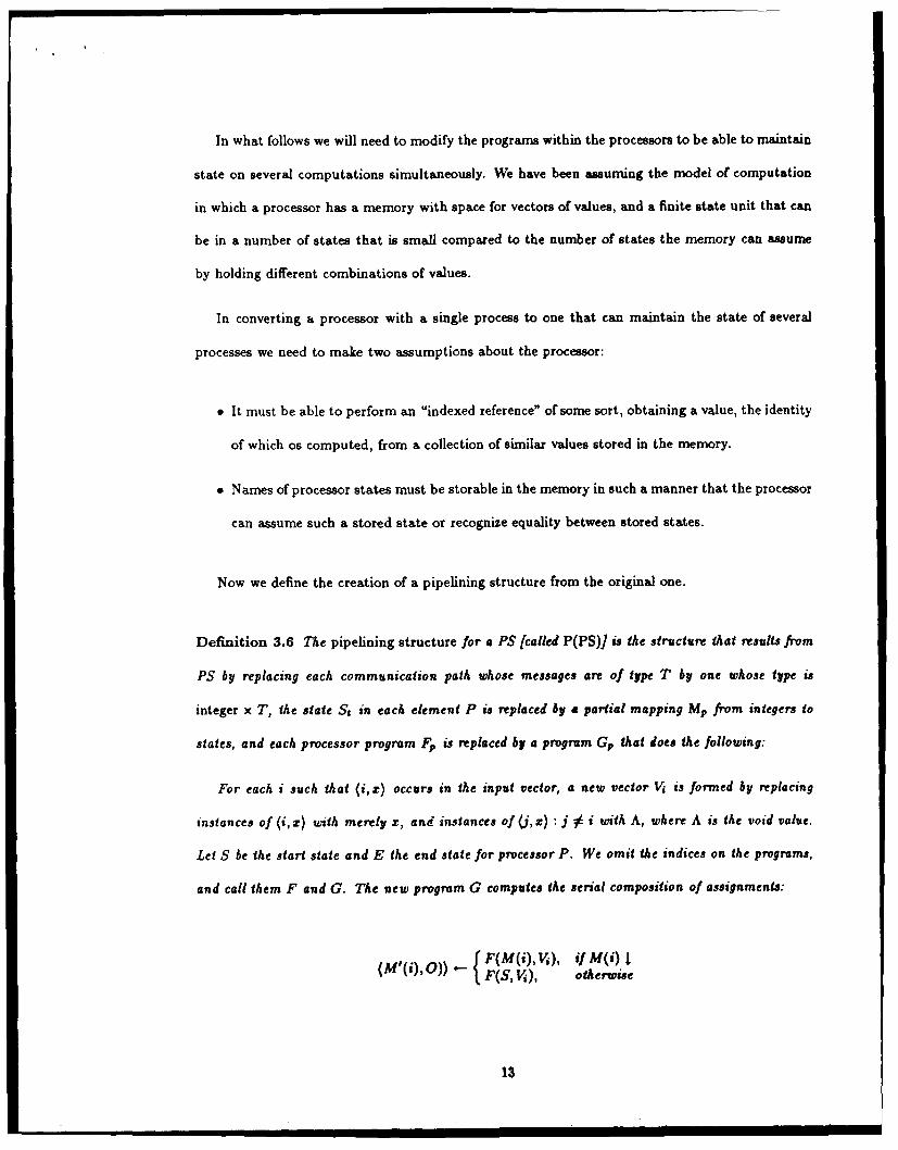
Definition 3.6 The pipelining structure for a PS [called P(PS)J is the structure that results from
PS by replacing each communication path whose messages are of type T by one whose type is
integer x T, the state S, in each element P is replaced by a partial mapping Mp from integers to
states, and each processor program F is replaced by a program Gp that does the following:
For each i such that (i, z) occurs in the input vector, a new vector Vi is formed by replacing
instances of (i, z) with merely z, and instances of (j, z) :j 9 i with A, where A is the void value.
Let S be the start state and E the end state for processor P. We omit the indices on the programs,
and call them F and G. The new program G computes the serial composition of assignments:
(M'i),)) F(M (i), V), if M(i) I
(MI(i),0)) - F(S, Vi), otherwise
13
and
M(i) , if M'(i) = E= MI(i) otherwise
and sends
A, ifi = A(i,z): z E 0, otherwise
Associated with a given processor P is a feasible output set FO(P), consisting of the outputs
which are available, given the history of input instances of P. Although many may be available, P
transmits in a given cycle that member (i, z) of FO(P), if any, with smallest label i.
There are several sets of data coursing through the PS at a given time, and it is necessary to
keep the various data and internal states straight to ensure that computations are performed on
corresponding input values and internal states. Hence the definition looks a little more complex
than it really is.
We will now show that P(PS) can solve multiple problem instances, under certain conditions,
provided that they are sufficiently separated in time.
First we get some preliminaries out of the way:
Definition 3.7 For a problem instance I for PS, P(I, i) is that problem instance for P(PS) ob-
tained by pairing all input, output and internal values for I with a unique integer label i.
So P(I, i) is intuitively just the problem I with the label attached to every input, internal
transmission, and result. This leads to the following easy result that tells us that this is the correct
definition:
14
Basic Observation 3.1 If PS solves a problem instance PI, then P(PS) will solve P(I, i).
Proof:
For every value v received by an element of PS the corresponding element of P(PS) will receive
(i, v), the corresponding state transition will take place in M(i), and therefore if the element of PS
would have transmitted w at some time, the element of P(PS) will transmit (i,w). I
Definition 3.8 The content C(PS) of a pipelining structure PS at a given time t is #{i: (3P E
PS)(Mp(i)) 1} (where we omit the time t for readability).
This definition says that the content of a structure is precisely the number of different labels for
which any processor is keeping a state. Since our definition of P(PS) keeps a state around for i in
a processor P only if computation on instance I has not finished, the content (pardon the pun) of
this definition is that the content of P(PS) at a given time is precisely the number of unfinished
problem instances in the structure somewhere.
We assume there is no overlap between parts of successive problem instances presented as inputs,
i.e. a problem instance is delivered in its entirety before a successor is begun.
Definition 3.9 The latency of a pipelined structure is the maximum (taken over all problem in-
stances) of the time interval between the entry of the first part of the instance into the structure
and the exit of the last part.
Definition 3.10 The separation of a stream of problem instances is the amount of time between
the start of transmission of successive instances.
Definition 3.11 The duty D(P) of a processor P is the number of transmissions it issues on any
single output line for E during one problem instance. The duty D(PS) of a PS is maxgepS[D(E)].
15
In our model, D(P) is proportional to the amount of time P is in use; we make this proportion-
ality constant 1 by appropriate choice of units.
We establish a lower bound to the separation of a stream of problem instances:
Basic Observation 3.2 Every PS with duty D has separation > D,
Proof: Let the latency be W, and the separation be S. After T time units, GJ + 1 problem
instances have been started, and all but [w1 + 1 of them, at most, have also been finished and
output. An element whose duty is D must therefore have delivered at least D(LkJI-( +1)
messages to the successor with which its duty is D. Note that D([MJ + 1 - > -I9-2
Let us assume S < D. Then there is a time To for which [D T W > To]. (This latter is equivalent
to observing that there is a To for which (D - S)To > D(W - 2S)) After time To + 2D, the element
whose duty is D is required to have handled more than Llk. problem instances, and therefore to
have made at least DT W transmissions on one of its lines. This is impossible, as DT&jY > To,
and only one transmission per time period may be made.
Basic Observation 3.3 Every PS with duty D takes > nD time to solve n problem instances.
Proof: This observation is a direct corollary of the previous one. g
Definition 3.12 The itinerary of a PS is that map I : integer - (multiset of processors) such that
if a problem instance is delivered at time t=O then exactly those elements in I(t) transmit messages
at time t. In cases where there will be no confusion, we will draw the itinerary as a sequence.
Definition 3.13 The activity of the PS is ji[#I(i)].
Note that 1(i) # 0 =:, 0 < i < activity(PS), because I(i) = 0 = I(i + 1) = 0, since in our model
every transmission is stimulated by a reception.
16
Basic Observation 3.4 For an itinerary I, activity(PS) <_ size(PS) -duty(PS).
This follows immediately from the definitions.
We have a lower bound of D[PS] for the separation of PS. Let D(PS) be D We now observe that
one can always build a pipelined structure with separation D+ 1. Specifically, given an itinerary for
the unpipelined structure, we can construct an itinerary for the pipelined version of that structure
that has certain desirable properties when fed a continuous stream of problem instances, namely:
" the separation of a stream of problem instances need not exceed D + 1;
" latency _< activuityxD;
" all iltenal queues have length < D;
* For a given time t, #{i :3P(Mp(i) T)) _< activity
The basic idea of the proof is to construct, for a given itinerary for the non-pipelined structure,
an itinerary for the pipelined structure. We shall proceed by interposing a number of skip steps
within the first itinerary. The number of skip steps between each transmission will be the same.
The number is chosen to be D, because a given processor P works on exactly DIP] different steps
in a problem instance, and hence at most that many different problem instances can present it with
input at a given time t (each must be at a different stage, since the problem instances are presented
to the input of PS in a staggered manner). Hence if we chose D skips, we will give time for P to
rompute , and the transmission line to transmit, all the values for the inputf' presented to it at t.
(Internal output to P, and internal output from P, are both buffered, by the FO(P) device).
Hence we take the first itinerary
(io, il,i 2 ,...) and add skips to create (io, A,A,...,ii,A,A,...,i 2 ,A,A,.... ), where there are
D many As in each gap.
17
Theorem 3.1 Suppose we have an indefinite stream of instances PPI = P(PI, 1), PPI2 =
P(P12 ,2), ... , presented to the inputs of P[PS in that order. Let S be the separation. Suppose that
S > D[P[PS]]. Then there is a bound B such that, for all times t, and processors P, #FO(P) < B.
This theorem states a condition on the separation of problem instances such that a given struc-
ture can handle an indefinite stream of problem instances. If we were to decrease the separation
below a tolerable limit, in our formulation this would show up as the phenomenon that FO(P)
increases without bound, i.e. that values are presented and computed faster than they can be
transmitted internally.
The proof proceeds by constructing an upper bound on the itinerary, such that the actual
itinerary is a refinement of the bound. A refinement of a function F whose values are multisets is
any function G such that for any argument z, G(z) C F(z), where C is multiset inclusion.
Proof: We call the activity of the structure A and the duty D.
Using W to denote multiset "union", define I' by
V'(i) I'(i) = reduce(tW, I), if i mod(D + 1) = 0
F'i = ~I(i) = 0, otherwise
By the definition of D, I' includes at most D instances of any single element. [The elements of I
are processor names.] The reason for
The folding of the itinerary corresponds to the propagation of multiple problem instances
through P(PS). Since each I'(i),imod(D + 1) = 0 is followed by D elements {I'(i + 1),I'(i +
2),... , '(i + D)), it will be possible for an element to transmit, in the D cycles following cycle
i, those values made necessary by receptions during cycle i or previously. Each value transmitted
during one of these D cycles will be received when or before it is scheduled to be received, which is
at cycle i + D+I.
Let the length of I be 1. For all processors P, all jI _I j < 1, all k > 0, if P E I(j) n times then
let n of the instances of P in I'(k(D + 1)) be assigned a problem instance number k - I + j. [Some
18
early instances of P will have negative instance numbers; transmit dummy values here.] Then I' is
a possible description of transmissions, together with problem instance numbers, that are feasable
if the problem instances are provided at D + 1-time-unit intervals. If a P is in I(k) then foral j
such that a transmission from another processor Q to P is in 1(j), j < i there will be an instance of
Q in 1(j), bythe construction. I
We now present the major theorem of this chapter, which is a summary of the two bound
observations. We have indicated a way in which a given serial structure may be pipelined, namely
by tagging a problem instance with a unique label (amongst active instances - one only needs at
most activity many labels), and providing buffering for each processor P so that only one output
for P is transmitted at once. The sets FO(P) are defined for that purpose. We could assume
instead that inputs are buffered internally to P. This will ensure the condition on P's outputs,
without FO(P). We would instead have FI(P) for the inputs. The condition is mathematical and
symmetric. The theorem says that this way is optimal for a given kind of pipelining structure.
In further chapters, we will indicate ways that this separation lower bound may be reduced, by
introducing multiple identical processors at certain points in the network, and connecting them to
the multiple output processors with specific topologies.
Theorem 3.2 Suppose PS has duty D and separation S. Then S > D and S may be chosen so
lhat S < D+ 1.
Proof: Immediate from Basic Observation 3.2 and Theorem 3.1.
There remians one step to complete the transformation. If you recall, an additional processor
was inserted to make the adjusted PS, in which it could be assumed that the transmission time
dominitaded the time each processor had to spend working on its part of the problem. This processor
is a "dummy" processor, which computes nothing and transmits nothing.
19

The pipeline structure will have no instances of this processor, because its duty is zero. The
wires will need to be removed. This is a natural consequence of the processor's insubstantial role
in the system.
20
Chapter 4
Systolic-Array Performance on non-Systolic Structures
4.1 Introduction
An appealing feature of systolic arrays is that for some problem classes it is possibl, 'o arrange
for problem instances to be supplied to the systolic array in such a manner that no connection
between any processor and the outside world transmits more than a single value during the solution
of a problem instance. When this condition and others are met it is possible to pipeline problem
instances, or supply one every time unit and, after a certain delay, obtain one result per time unit.
We wish to explore ways of making pipelined structures out of nonsystolic structures. A pipelined
parallel structure is one whose various processors can usefully be working on different instances of
one problem at the same time, so several problem instances are in the structure when the results
from the first one emerge.
21
4.2 Utility Of Pipelines
Pipelining is principally useful in two cases. In this description I will assume that a short
separation is desired; if a long separation and latency are both acceptable it is reasonable to supply
only a single processor and not use concurrency at all.
One case is the reduction of the total memory-time product required for a computation by
arranging for portions of the computation to take place in different processors of the structure.
This occurs when different problem instances share some of the input; instead of arranging for
a partially-redundant complete problem instance to reside in each of several processors solving
different problem instances that share data, a single copy of this data is spre:a among all of the
processors, each solving the same part of all of the instances. Perhaps the best-known example
of this is matrix multiplication, which multiplication of n x n matrices can be thought of as n
multiplications of n-element vectors by n x n matrices.
This motivation for pipelining will not be discussed further; while it can be important, the
types of structures that tend to result have been considered by us previously. As in the matrix
multiplication example, a situation in which multiple problem instances with some data shared
arises can often be regarded as parts of a larger problem.
A second case, the case we discuss here, is that in which the purpose of pipelining is to secure
a short separation interval.
Pipelines are not useful when a user wants a low separation but can tolerate a very long latency.
In this case, concurrency should not be used on any single problem instance; instead, a large number
of processors could be provided, disconnected from each other except that each can receive problem
instances from the source and can deliver results to the destination. They can be used in rotation,
like the barrels of a Gatling gun, to deliver a flow of solved problem instances more frequently than
one unit could. The descriptions of some problem instances, or of the results, may be too bulky to
22
be delivered to a single processor within the desired separation; this can be overcome by providing
a serializer or deserializer on each processor.
Pipelines are useful where a low separation and a low latency are both desirable. There are the
obvious cases such as real time applications; there are also cases in which the results of some of the
early runs are used to modify the input data for some of the later ones, or to make computation of
some of the later instances unnecessary.
An important non-real-time case where this can occur is where the multiple problem instances
are really parts of a larger problem.
4.3 Pipelining "Nonpipelinable" Structures by Duplicating Processors
Many of the computational problems that must be solved in any system must be solved re-
peatedly. A real-time example might be an aircraft, doing situation recognition of any form; a
non-real-time example might be a series of problem instances (with slightly differing data).
As one example of what might be possible, we consider the dynamic programming structure
of [King85]. We describe below the problem and the solution of that paper, and we show the
structure graphically in Figure 4.1.
The class of dynamic programming problem solvable by that structure is that class in which
1. a problem instance is an ordered sequence of items
2. the result for a sequence of length 1 can be determined simply
3. F(S) = reduce(@, {F(S) e F(S 2 )ISI IIS2 = S}), where 9 is an associative and commutative
binary operator, e is an appropriate binary operator, and II is concatenation.
23
P41
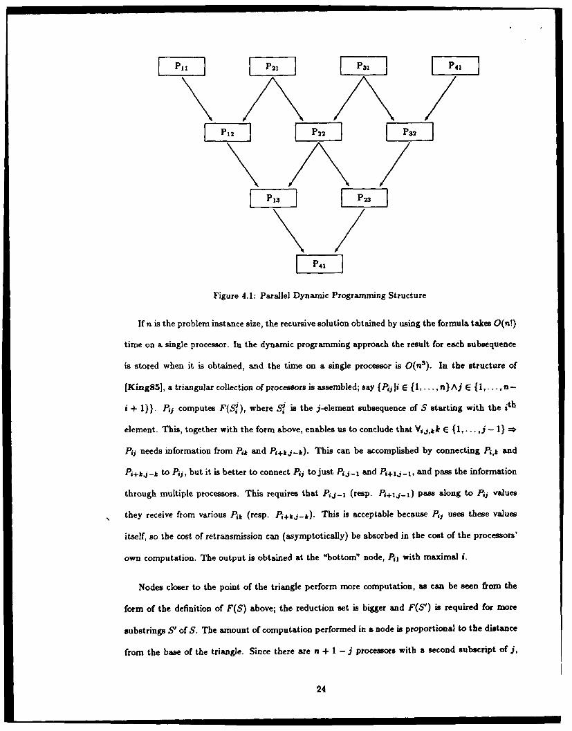
Figure 4.1: Parallel Dynamic Programming Structure
If n is the problem instance size, the recursive solution obtained by using the formula takes O(n!)
time on a single processor. In the dynamic programming approach the result for each subsequence
is stored when it is obtained, and the time on a single processor is 0(n 3 ). In the structure of
[King85], a triangular collection of processors is assembled; say {Pji E 1... , n} Aj E {1,., nh-
i + 1)). Pjj computes F(S ), where S is the j-element subsequence of S starting with the ith
element. This, together with the form above, enables us to conclude that Vij,kk E {1, .. ,j - 1} =*
Pij needs information from Pk and P+kj-k). This can be accomplished by connecting P,k and
Pi+kj-k to P,, but it is better to connect Pq to just Pjj-j and Pi+lj-1, and pass the information
through multiple processors. This requires that Pj- 1 (resp. P+ 1,,j- 1 ) pass along to Pj, values
they receive from various Pk (resp. P+kj-L.). This is acceptable because Pi, uses these values
itself, so the cost of retransmission can (asymptotically) be absorbed in the cost of the processors'
own computation. The output is obtained at the "bottom" node, Pil with maximal i.
Nodes closer to the point of the triangle perform more computation, as can be seen from the
form of the definition of F(S) above; the reduction set is bigger and F(S') is required for more
substrings S' of S. The amount of computation performed in a node is proportional to the distance
from the base of the triangle. Since there are n + I - j processors with a second subscript of j,
24

and each one performs 11(j) units of computation, the total amount of computation performed by
approximately - processors is approximately zT units, over 2n time units. If every processor were2
2 3
fully occupied 2n time units would suffice to complete 2n-- = n internal computations, enough
to solve six problem instances.
If we were to attempt naive pipelining, which is accomplished by merely making a second problem
instance available to the base of the triangle as soon as the first instance was absorbed, we would
halve the separation; it is impossible to do better because the amount of data transferred through
the bottom node, the busiest processor, and the amount of computation it must do, takes half of
the time that it takes the whole structure to solve a single problem instance. We therefore get only
one third of the computation power from the processors we provide; we have enough computation
power to solve six instances, but we can only handle two.
The reason for this low efficiency is simple. In this structure, most processors do much less work
than is done by the single processor at the apex of the triangle. For example, the processors at the
base of the triangle each perform no computation, and one transmission in each of two directions.
What we would like to have is more computation power, strategically placed in the computation
network, so all of the network is kept equally busy by an indefinite stream of problem instances.
In this example, we would like nodes whose second subscript is j to have j times as much commu-
nications and computation capacity as the nodes at the base of the triangle, since it has j times
as much work to do. This would make the entire network able to handle one problem instance per
time unit, at a cost of providing ! units of processing power.
However, this is unlikely to be the best way to proceed, since this leads to fewer processors doing
more work. It is well known that in general it is much more efficient to have more processors, each
doing less work, than the other way around.
25
4.4 Problems with Pipelining
The loss of efficiency does not derive merely from the high separation necessary. In the ideal case,
if the separation is s and the required computation is c we will only need ,£ units of computation
power. If we need to reduce the separation to s', we can provide r,'71 duplicate instances of the
structure; using them in parallel by distributing [evenly] the incoming problem instances.
The problem with the triangular structure above, and others, is that there are some processors
that have more activity than others. We want the activity to be distributed evenly to make the
best use of our computational resources. In the pipeined case, we also want to maximize the mean
activity level.
4.5 Mitigation Strategies
If the structure that results from a concurrency synthesis is imbalanced, balance can be restored
by multiplicating some of the processors. Basically, if the desired separation is S, but a processor
P has a duty of D, r-j copies are made of P. Let c = rQi. We call these multiple processors a
column; denoted by CP. The column of c processors can be thought of as a single more powerful
processor capable of doing that work that was done by P, in D time, for c problem instances instead
of one. Since C > , the column achieves a performance as good as or better than one problem
instance every S time units over a sufficiently long time interval.
Definition 4.1 A columnization CPS of a parallel structure PS is a structure in which each
processor of PS has been replaced by a column, described above. Each processor in the column will
do what the corresponding processor of the original structure did. Ezactly those pairs of columns
that correspond to a pair of processors that were connected by an edge in the original structure will
be connected by a network, possibly with switches, to be described below. We will rfer to the column
replacing the processor P as CP, and to individual processors of CP as CP , CP 2 ,... ,CP', where
I is the number of processors in the column, called the length of the column.
26
This should be distinguished from the virtualization of [King85]. In virtualization, a loop of
one processor's task per problem instance is replaced by a series of accesses to a partial result ad
creation of a new partial result with a higher index. In this, the processor's chore is the same before
and after columnization;
Definition 4.2 If processors P and Q are columnized into columns CP and CQ respectively, CP
feeds CQ if there is an edge from P to Q. CP is the source and CQ is the target.
We will require that in a columnization all data pertaining to one problem instance be delivered
to only one processor in each column. We call this requirement the Distribution Requirement [DR].
For the purposes of these definition a pair of processors P and Q such that P sends information
to Q and Q sends information to P is considered to be connected by two edges.
Given that processor P1 is replaced by column C and P2 has been replaced by C2 , and that
there was an edge from P to P2, we now must say what network replaces the edge.
Some networks have multiple paths from the column replacing the source processor of the edge
to the one replacing the target. In this case we shall require switches for a given input/output
processor pair. The switching protocol will normally be dependent on the topology of the original
parallel structure.
27
4.5.1 Interfacing Columns of Processors
When we consider interfacing two columns, one of which feeds the other, we will assume that
the DR is satisfied for the source, and we need to ensure that it will be satisfied for the target. We
call a method for doing this a Distribution Strategy.
Let us consider a simple case, which may generalize:
Definition 4.3 A FIFO with capacity C is a memory with capacity C that
" has an input and output terminal
" signals to the object connected to the input terminal that it is ready for data whenever it
contains fewer than C data
" whenever the object connected to the output terminal signals that it is ready for data, and it
contains any data, sends and erases [ceases to contain] the oldest datum it contains
It will usually be obvious from context what connections are in force whenever we say "a FIFO
of capacity C exists between points a and b. We will now describe one possible connection network
between columns C and C'.
Definition 4.4 Suppose columns C and C' have length I and I' respectively. WLOG say 1 < i' and
' - 1 = d. Further suppose that each processor P of the target column has a FIFO buffer with
capacity D(P), where P is the processor whence C. The terminals of the source column are
the outputs of the FIFOs, and the terminals of the target column are the processors' natural input
terminals. Narrow Fanout columnization is a columnization in which the interface network which
for each i < I there is a switch and wire that can direct information from the terminal for C' to
O+' for 0 < j < d
28
A narrow fanout columnization allows several problem instances to be distributed to fresh
processors within the interval corresponding to a single processor's duty, without reducing the
duty of any processor. The latter is something we will not attempt to do.
Narrow fanout columnization can be used to ease bottlenecks that could otherwise exist is a
pipelined stricture if a switching protocol which we will describe below is used.
In the theorem below we will show that a small improvement in the separation of a pipelined
structure can be achieved by using narrow fanout columnization between one particular pair of
columns. While this improvement will be small, it is cumulative; in certain cases the separation of
a parallel structure PS can be reduced from D(PS) to 1 by reductions to D(PS)-1, D(PS)-2,....
Theorem 4.2 would appear to be impossibly narrow, but one example in which its conditions
are met is the case of a chain of processors, with processor i connected exactly to i + 1 except at
the ends of the chain.
Another place where the theorem needs to be broadened is the conditions on the communication
within the halves of the original paralel structure that are joined by the single edge of the Theorem.
It must be true that the entire problem instance is available at immediately sequential times after
the first output is available from the source processor. It must also be true that the target processor
can immediately generate all elements of its output on any problem instance on which it has started
to deliver output.
Definition 4.5 A major cycle is an i-time-unit interval at the beginning of which an output which
is the first for problem instance m is made available by some members of CS. WLOG we will
assume that CS delivers a complete problem instance every major cycle - we can provide dummy
instances for members that do not provide real ones.
29
t=0 9=3 t=6 f=9
C2CT 3 C5 CT 3 F F(W = 0) (W a 1) J
C3CT' S CT' CT3(W = 0) (WM 1. 2n)
t=12 t=15 t-18 t=21
CS C1
(iO ,L j 2 3
C52 CT2 C82 CT32
(W . 2) (W* ) i L.J J.~
CT4
) CT3 CT3CS(W = )(W - )(W.=2
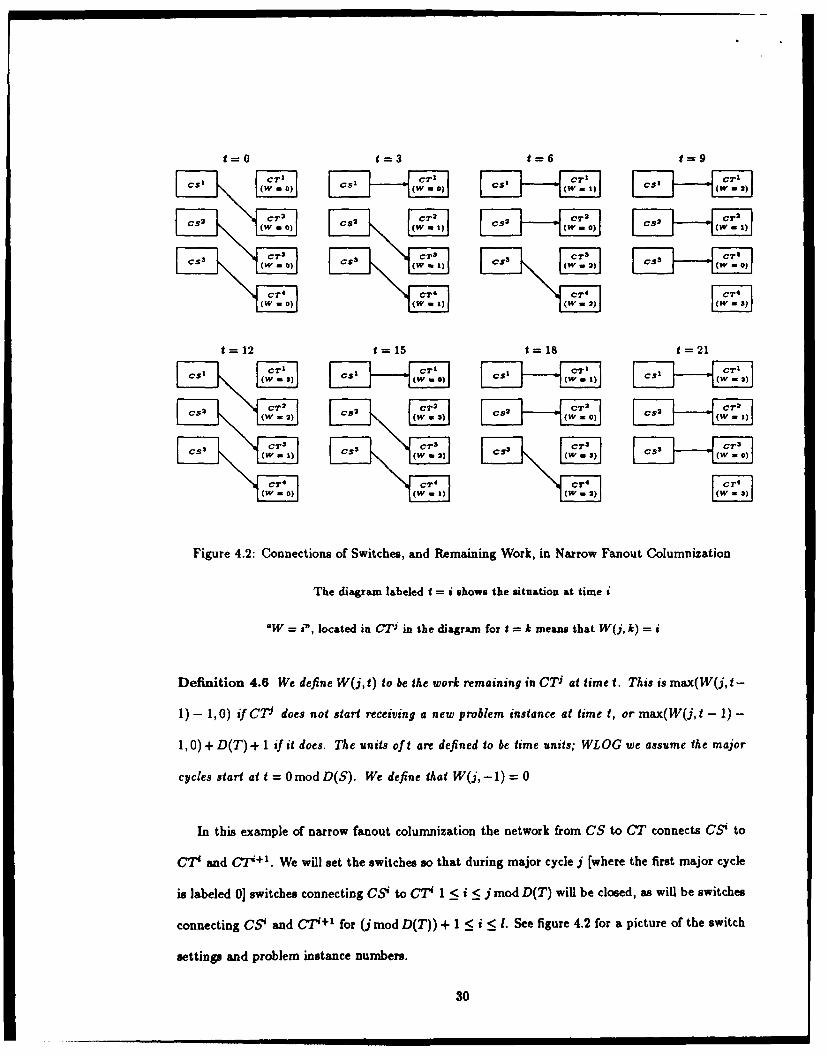
Figure 4.2: Connections of Switches, and Remaining Work, in Narrow Fanout Columnization
The diagram labeled f = i shows the situation at time i
"W = P,' located in CTJ in the diagram for t = k means that W(j, k) = i
Definition 4.6 We define W(j,t) to be the work remaining in CV at time t. This is max(W(j,t-
1) - 1,0) if CT does not start receiving a new problem instance at time t, or max(W(j,t - 1) -
1, 0) + D(T) + 1 if it does. The units of t are defined to be time units; WLOG we assume the major
cycles start at t = 0modD(S). We define that W(j,-1) = 0
In this example of narrow fanout columnization the network from CS to CT connects CSi to
CT and C74+ '. We will set the switches so that during major cycle j [where the first major cycle
is labeled 0] switches connecting CSi to CT 1 < i < j mod D(T) will be closed, as will be switches
connecting CS' and CT + 1 for (j mod D(T)) + 1 < i < 1. See figure 4.2 for a picture of the switch
settings and problem instance numbers.
30
--.. .ran .. ,,.,,,,= i n I i ii nlmmi • i
Lemma 4.1 CP receives a problem instance during exactly those major cycles during which i #
jrmodD(T). If i< jmodD(T) then CS' sends an instance to CT; if i> jmodD(T) then CS"-
sends an instance to CT; if i = jmodD(T) then no instance is delivered.
Proof: All switches leading from CS', i < j are aimed at CT; all switches leading from CS', i > j
are aimed at CT+'; If CS j exists its switch is aimed at CT' + ', and if CSj - ' exists its switch is
aimed at CT - 1 . I
Below we consider the columns CS, resulting from a processor S with duty D(S), and CT,
resulting from a processor T with duty D(T). D(T) = D(S) + 1. The original structure has an
edge from S to T. To get full use from all of the processors in a column, we need to ensure that:
1. Every column resulting from a processor that outputted to S in the original structure is at
any time to transmit to some processor in CS, although it need not always be the same one.
2. CS can deliver a total of D(S) problem instances to its outputs in D(S) time units.
3. A processor of CS will be finished delivering one problem instance before it is required to
begin another by condition 2., immediately above.
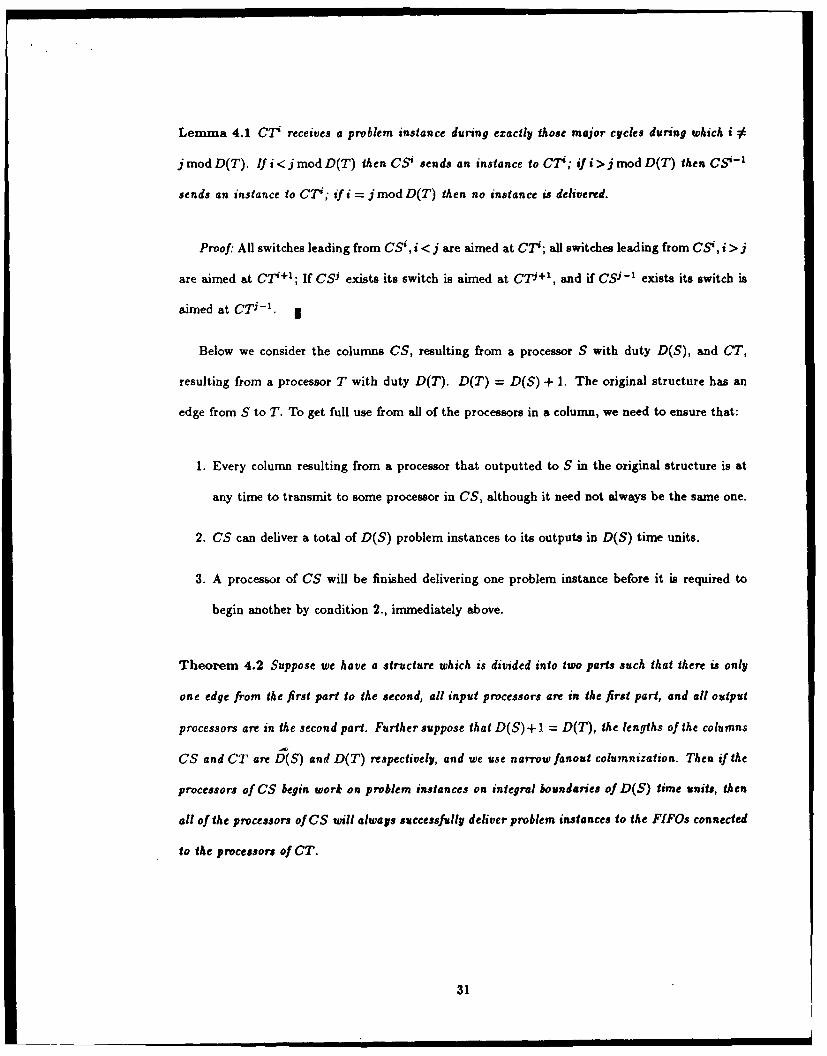
Theorem 4.2 Suppose we have a structure which is divided into two parts such that there is only
one edge from the first part to the second, all input processors are in the first part, and all output
processors are in the second part. Further suppose that D(S)+I = D(T), the lengths of the columns
CS and CT are D(S) and D(T) respectively, and we use narrow fanout columnization. Then if the
processors of CS begin work on problem instances on integral boundaries of D(S) time units, then
all of the processors of CS will always successfully deliver problem instances to the FIFOs connected
to the processors of CT.
31
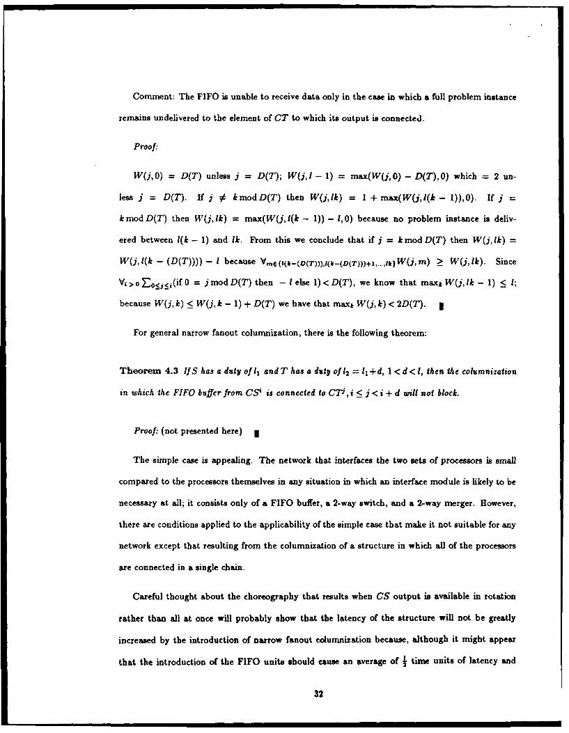
Comment: The FIFO is unable to receive data only in the case in which a full problem instance
remains undelivered to the element of CT to which its output is connected.
Proof:
W(j, 0) = D(T) unless j = D(T); W(j, I - 1) = max(W(j, 0) - D(T), 0) which = 2 un-
less j = D(T). If j 96 kmodD(T) then W(j, ik) = 1 + max(W(j,l(k - 1)),0). If j =
k mod D(T) then W(j, lk) = max(W(j, l(k - 1)) - 1,0) because no problem instance is deliv-
ered between i(k - 1) and lk. From this we conclude that if j = k mod D(T) then W(j, 1k) =
W(j,l(k - (D(T)))) - I because VmE{,(k.-(D(T))),I(k-(D(T)))+I, ... ,IkW(j,m) >_ W(j,lk). Since
Vi > oE 0 <j<i(if 0 = jmodD(T) then - Ielse 1)<D(T), we know that maxkW(j, lk-1) < i;
because W(j, k) < W(j, k - 1) + D(T) we have that maxk W(j, k) < 2D(T). *
For general narrow fanout columnization, there is the following theorem:
Theorem 4.3 If S has a duty of l and T has a dulty 0fl2 = 11 +d, 1 < d < 1, then the columnization
in which the FIFO buffer from CS' is connected to CT, i < j < i + d will not block.
Proof: (not presented here) j
The simple case is appealing. The network that interfaces the two sets of processors is small
compared to the processors themselves in any situation in which an interface module is likely to be
necessary at all; it consists only of a FIFO buffer, a 2-way switch, and a 2-way merger. However,
there are conditions applied to the applicability of the simple case that make it not suitable for any
network except that resulting from the columnization of a structure in which all of the processors
are connected in a single chain.
Careful thought about the choreography that results when CS output is available in rotation
rather than all at once will probably show that the latency of the structure will not be greatly
increased by the introduction of narrow fanout columnization because, although it might appear
that the introduction of the FIFO units should cause an average of " time units of latency and
32
could cause 21, this will not actually result because when information is available before it is needed
for the theorem, the connection can be established and used early because the target processor will
probably be ready to receive it only d time units after the infurmation is available.
4.5.2 A More General Balancing Strategy
We now consider a more general connection network between two columns of processors.
We recall the Distribution Requirement, which is that even where there are two paths by which
information pertaining to a problem instance can arrive at a column CT, we must arrange for all
of that information to arrive at the same element of that column. If the length of CT is 1, a simple
strategy for meeting that requirement is to arrange for instance i to be processed by processor
CT mod I
Definition 4.7 A complete crossbar columnization network is a network between two columns in
which any bipartite matching between the processors of the two columns is realizable as a connection
through the network.
This form of columnization network is named after the well-known network called a crossbar
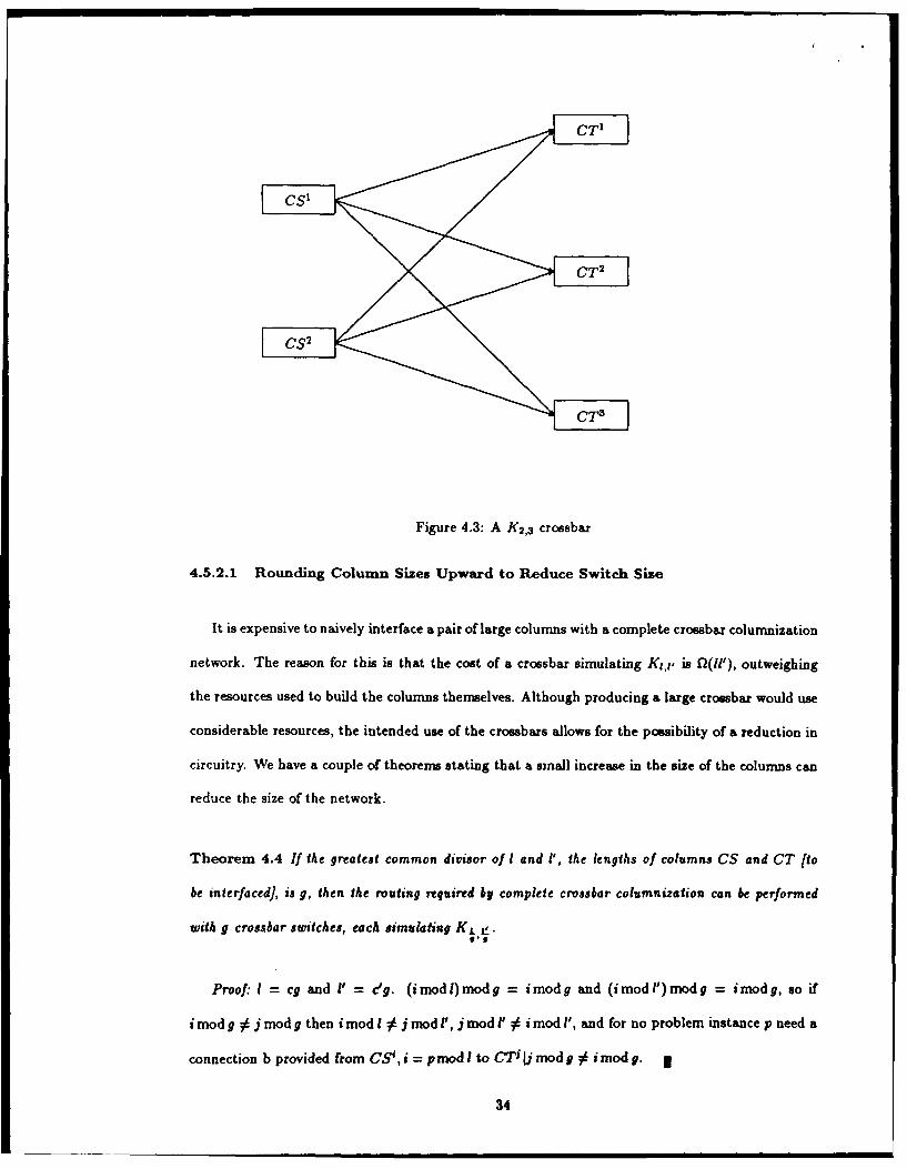
which has an analogous property. An example of such a network can be found in figure 4.3.
Implementing an n x m crossbar is well-known to take O(nm) switches, unless superconcentratcrs
[or equivalent] are used. Superconcentrators are unreasonably expensive unless n and m are very
large, compared with most problems.
33
CT 1
Figure 4.3: A K 2 ,3 crossbar
4.5.2.1 Rounding Column Sizes Upward to Reduce Switch Size
It is expensive to naively interface a pair of large columns with a complete crossbar columnization
network. The reason for this is that the cost of a crossbar simulating K1 ,1, is fQ(l'), outweighing
the resources used to build the columns themselves. Although producing a large crossbar would use
considerable resources, the intended use of the crossbars allows for the possibility of a reduction in
circuitry. We have a couple of theorems stating that a small increase in the size of the columns can
reduce the size of the network.
Theorem 4.4 If the greatest common divisor of I and 1', the lengths of columns CS and CT [to
be interfaced], is g, then the routing required by complete crossbar columnization can be performed
with g crossbar switches, each simulating K1 .
Proof: I = cg and I' = e'g. (imodl)modg = imodg and (imodl')modg = imodg, so if
i mod g 6 j mod g then i mod 1 6 j mod ', j mod I' i i mod 1', and for no problem instance p need a
connection b provided from CS',i = pmod I to CT" j mod g 6 i mod g. *
34
CT'
CT 2
CS35
CS4C e
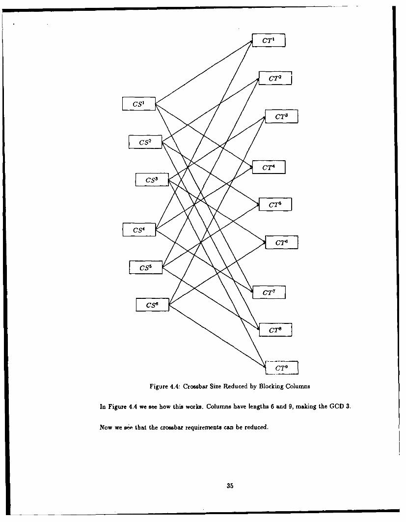
Figure 4.4: Crossbar Size Reduced by Blocking Columns
i In Figure 4.4 we see how this works. Columns have lengths 6 and 9, making the GCD 3.
Now we se that the crossbar requirements can be reduced.
35
Theorem 4.5 If the cost of implementing a i x j crossbar is cij, and the greatest common divisor
of i and j is g, then the cost of implementing the crossbars required by crossbar columnization of a
pair of columns of lengths i and j need only be _I
Proof: By the previous theorem, a processor CSk may need to communicate with C7'" iff
k mod g = m mod g. For each equivalence class under mod g, there are processors in CS and 'processors in CT. The required crossbar is therefore x , requiring ci - = c cost. g of these
crossbars are required, for a total cost of cL.|
We need not depend on luck or benign problems to make adjacent columns' lengths share a large
common divisor. We can, instead, increase the sizes of columns to make this happen. If we made
the columns' lengths all be powers of two, for example, all pairs of columns could be interfaced
by 1 x 2 "crossbars" [actually single switches) at the cost of an increased number of processors in
the columns. There are less extreme rounding formulae, but a consistent policy must be followed
within a parallel structure to avoid "seams" between regions of distinct rounding policies.
There are optimization problems implicit in the varying ratios of switching element cost and
processor cost within the parallel structure, and the constraint that regions of differing rounding
policy can only be joined by columns in which the two policies happen to lead to the same result.
Solving these problems in in the realm of future work.
4.5.2.2 Little Increase in Latency
In the crossbar case we show (below) that the increase in the latency of the network will be
small, comparable to the difference between the lengths of the columns when the destination column
is the larger. The key point in the proof is that it is possible to connect to the target processor as
soon as it is finished with its previous work.
36
Theorem 4.6 Suppose we have columns CS and CT, with CS having length I and CT having
length 1'. Further suppose processors S and T duties of I and 1', respectively. Yet further suppose
that problem instance j + 1 comes to be available at least one time unit later than problem unit j,
for all j. Then processing of problem instance j by CTj mod ' will be able to begin as soon as the
information is available at the interface between CSj mo'4 and the network between CS and CT.
Proof: by induction on j. Base case: Obviously the theorem is true for any j _ ', because no
processor of CT will be working on a previous problem instance when it comes to be time to deliver
problem instance j; k < j [k mod l' = j rod I]
Induction step: Since the statement is true for j'< j, in particular it is true for j' = j - 1'.
Problem instance j' was the last problem instance to be delivered to CT j md "' . Since it was
delivered I' time units ago, it is completed; CTj modI' is therefore ready for problem instance j.
4.5.3 Using a "Shifter"
If we synchronize the outputs of a column, we find that all elements of the smaller column are
connected to a subsequence of the larger column [defining "subsequence" using modular arithmetic].
This is precisely the behavior of a "shifter", and we can borrow from techniques for implementing
these to perform interfacing between columns. Without loss of generality, we describe the situation
in which the output column is the longer one, but a structurally similar one will work in the opposite
case. If the length of the longer column is 1, a series of switching units can be provided; the first will
send inputi to output i or to output+j mod 1 ; the second sends inputi to output, or to outputi+2 mod 1;
etc. through logI stages, with the jth stage performing either no shift or a shift of 2j -I depending
on the switch settings.
An advantage to this network is that it is less expensive to implement than a crossbar colum-
nization network, but a disadvantage is that the latency contributed by a column interface will be
longer, due to the fact that an entire shifter must be reset simultaneously.
37
This method of building shifters is well known, and creates a network with a propagation time of
£(log 1) and use of switching resources fQ(! log 1). As we will soon see, this delay and resource use is
insignificant in this case, but only because of the large delay intrinsic in the use of this arrangement.
The latency accounted for by this particular communications network in a larger system is fQ(l)
[specifically L minimum, 21 maximum]. This results from the fact that the communication must
actually be synchronized, unlike the previous cases in which the synchronization ability is only
provided to meet the needs of the theorems. The reason for this is that the shift offset of the
interconnection network must all be changed simultaneously.
4.6 Comparison of the Three techniques
We will consider computation and transmission to be the costs of a structure. A structure wil
also require memory within the processors and the FIFOs, but we will not consider memory cost
at this time because the cost of memory is currently so small. We may want to reconsider this in
the future if this changes.
4.6.1 Narrow Fanout Columnization
Where applicable, narrow fanout columnization with a small difference uses minimal latency,
wiring, and network logic. The conditions of applicability that we have found so far are rather
narrow, but we conjecture that they can be broadened.
38
4.6.2 Crossbar Columnization
In crossbar columnization, we can "trade off" a smaller interface network for somewhat larger
columns than would otherwise be required. If the natural column lengths of the problem are used,
frequently a full crossbar need be provided to interface adjacent columns. As one example, in the
dynamic programming structure of [King85], adjacent columns will have lengths that differ by 1,
insuring that there is never a common divisor greater than one that allows anything else to be
used. Since the provision of that much crossbar would make the network for computing dynamic
programming problems of n inputs with unit time separation require 2(n4 ) components.
The "rounding up" approach described above is very effective. Consider the simplest version,
in which the length of each column is rounded up to the next higher power of 2. In the worst case,
every columns will be twice as long as it should be for the duty of the replaced processor, and the
amount of network circuitry is the same as in narrow fanout columnization.
More generally, if the column length is rounded up to the next higher number of the form
i2j, I < i < c for constant c and for i and j both restricted to be integer-valued, then no column
will be longer than it should be for the duty of the replaced processor by a factor of more than C+2
if c is even, or if c is odd. In exchange for this increase in column length, the amount of network
circuitry can be c - 1 times the amount required for narrow fanout columnization [assuming that a
switch that directs an incoming signal to one of n outputs takes an amount of circuitry proportional
to n - 11.
4.6.3 Shifter Colurnnization
We believe the latency of a parallel structure including shifter columnization is significantly
larger than that of the other forms; not because of the logl depth of the network, but because of
the need for synchronization which we conjecture is not shared by the other two.
39
4.7 Open Problems
We have shown a variety of techniques to make efficient pipelining structures from structures
that would normally not pipeline well. The basic reason for lack of pipelining is the existence of
a few processors that have duties, or amounts of work or communication to perform, in excess of
some other processors. The technique of choice to improve pipelining is to replace each processor
that is overly busy by a column of processors, each capable of performing the work of the replaced
processor, in sufficient quantity to achieve the desired throughput.
There are some unanswered questions we would like to answer.
4.7.1 Extend Utility of Narrow Fanout Columnization
The main problem with using narrow fanout columnization to meet the bulk of the interfacing
needs with respect to connecting two columns of processors is that the mapping of problem instances
to processors within a column is dependent on non-locally-determinable factors. If instance i
is processed by CSJ, it must be processed by CTj or CT j +l, a requirement inconsistent with
processing it in processor C rood '.
Suppose there are two trails of columns leading back to input columns, but the sequences
of lengths of the columns on the two trails are not identical, then a series of narrow fanout
interface networks would deliver parts of one problem instance to different processors in the
target column. Consider, for example, the following example: there is a trail from CA to
CB to CC to CF, and one from CA to CD to CF. length(CA) = 1, iength(CB) = 2,
length(CC) = 3, length(CD) = 2, and length(CF) = 4. We therefore have two chains, one
of whose columns have lengths 1, 2, 3, and 4 and the other of whose columns have lengths 1,
2, and 4. Working out the processor assignments we see that as transmitted through the first
(longer] chain the stream [(1), (2), (3), (4), (5), (6), (7), (8)] becomes [(1, 2), (3,4), (5,6), (7,8)] in CB,
40

[(1,2,4),(3,5,6),(7,8, A)] in CC, and [(1,2,4,6),(3,5,8, A), (7, A, A)] in CF. The other chain does
have [(1,2),(3,4),(5,6),(7,8)] in CD, but it becomes [(1,2,3,4),(5,6,7,8)] in CF.
4.7.1.1 Discovering Paths with Common Column Length Sequences
For some structures this problem does not arise because all paths from any input column to a
given column have the same sequences of lengths. In this case the sequence is (1, 2, 3,. .. , 1) where
I is the length of the target column. In this case a proof is easy to craft from the observation that
the interconnections of the original structure are all from nodes that deserve columns of length i to
ones deserving columns of length i + 1; we want to derive some more general results.
4.7.1.2 Making Paths with Common Column Length Sequences by Padding
We conjecture that there are cases in which all paths from input to any node are of the same
length, but there are different natural column lengths (based on the original processors' duties)
along these paths. If this is so, it might be possible to extend the shorter columns by adding
otherwise unnecessary processors to those columns. We need to find out where this works and is
productive.
41
4.7.2 Folding Together Narrow Fanout Columnization and Other Types of Colum-nization
A problem with using narrow fanout columnization and other types in the same structure is
that the other types of colurn'izaticn assume that in a column of length 1, problem " str.,c i will
be delivered to processor i mod I in the column.
Suppose there is a region p of a parallel structure all of whose inputs are (or can be, with
reasonable padding) of the same height, and all of whose outputs are also of the same height, but
within which there are paths with disparate column length sequences. Then the region cannot be
built from narrow fanout columns.
Further suppose that for each node in the structure, all paths from inputs to that node through
which data actually flow go through the region the same number of times.
Then it will be possible to use crossbar columnization in p and narrow fanout columnization
outside that region, provided that there is no path component outside of p with disparate column
length sequences.
We need to find methods for determining such regions, making them as small as is possible to
reduce the amount of resources necessary for crossbars. In what follows we will call these regions
moats.
4.7.3 Optimize Crossbar Columnization
The observation that crossbars can be smaller but more numerous, and therefore consume
less resources, when the greatest common divisor is larger than when it is smaller, leads to an
optimization issue as we have discussed above. This issue is made somewhat more complex when
the fact that there are "competing" forms of columnization available is noted.
We need to develop optimization criteria for this technique.
42
4.8 Future Work
As we have seen, it is useful to balance a concurrent structure by providing "assistants" to those
processors that carry a disproportionate share of the computation load. If this is done the structure
can Pioeline, and all of the processors are kept fully busy. We would then fall short by only a small
constant factor (inherent in the construction of a pipeline structure from an ordinary concurrent
one - see Chapter 2) of achieving full processor utilization. We have shown that by colurnization,
or provision of duplicate processors for heavily used ones and using all processors of a given type
in rotation, we can meet this criterion. We have also described several types of columnization.
Crossbar Columnization is clearly the most general, although the most expensive, form of colum-
nization. Any problem amenable to these techniques at all can be handled in this manner. This is
the most expensive structure, however, requiring additional processors and a moderately expensive
switching network.
Above we described techniques for reducing the expense of this form of columnization, and
techniques for and conditions under which the less expensive ones can be used. Work remains to
completely describe and develop the technique.
4.8.1 Generalization of Narrow Fanout Columnization
Theorem 4.2 states that if there is only one edge between two parts of a structure that need to
process problem instances at different speeds, a certain simple and inexpensive network can be used
to match the needs. This theorem is extremely narrow, yet we suspect broadening to be possible
along several fronts. For some parallel structures the information sent out by one processor for
one problem instance cannot be sent contiguously [without intervening values for other problem
instances) without artifically increasing latency. This will occur whenever the information sent from
one processor to another in the structure is not contiguously sent.
43
It still seems likely that the data can be properly interleaved so narrow fanout columnization
can still be used, but we do not yet have a proof of this conjecture. We want to create one.
This is the cheapest form of columnization. It achieves its low cost by restricting the choice
of problem instance paths to the minimum necessary to insure that every element of the longer
column communicates with at least one element of the shorter, and that the number of longer-
column processors each processor in the shorter column communicates with is equal.
This restriction has the consequence that after a chain of networks built for narrow fanout
columnization the assignments of problem instances to processors cannot be predicted without
detailed knowledge of the paths taken to get to the particular column.
This, in turn, has the consequence that whenever several streams of data converge on one column
some special care must be taken to insure that data arriving at a single processor all comes from
the same problem instance.
In future investigation we should be able to validate the following techniques:
e Isolation of cases in which the correspondence will work because the data has the same history
of passage through equivalent narrow fanout column interface networks
* In cases where that is impossible, provision of conversion networks to make the problem
instance assignments match. Minimize their number.
44
4.8.2 Combine Narrow Fanout Columnization with Other Columnizations
We have described above a situation in which "most" regions of the pipelined concurrent struc-
ture meet the criteria for direct use of narrow fanout columnizations, but a small region doesn't.
The technique we will explore is isolation of such regions, given the description of the structure.
To use this technique we can isolate and use "small" regions for which every path from a node
receiving information from the outside world to any node N of the pipelined structure passes
through the region the same number of times as any other path from any information-receiving
node to N.
The work that must be done here [beyond finding "straight" narrow fanout columnizations]
includes:
" find heuristics for isolating moats, or regions which satisfy the path condition for supplement-
ing narrow fanout columnization.
* determine, for such regions, what nodes they cover.
4.8.3 Improve Crossbar Columnization
The optimization problem here is choosing an amount by which to "pad" the columns to reduce
the size of the network. Recall that the reason for increasing the column length beyond that which
would be required by the replaced processor's duty is to increase the greatest common divisor of
the lengths of two columns which share communication, in order to allow the interfacing network
to be a large number of little crossbars instead of a few large ones or one huge one.
Given that the cost of an n x m crossbar is assumed to be f0(nm), say cnm, if the length of one
of the columns is fixed and the ratio of the cost of a processor to c is known it is simple arithmetic
to choose a column length. This is even true if neither column length is fixed but there are minima
on both.
45
It becomes a more complex problem coordinating the lengths of all columns. We have done little
in this area, but we expect that a "greedy algorithm", addressing the columns in order of some
function of the ratio of the cost of their processors to c, would work reasonably well. Intuitively
the columns that are full of expensive processors [and their neighbors] should be addressed first,
and this seems to work reasonably well on examples we have tried by hand, including two adjacent
columns of mutually prime, large, approximately equal length, with extremely expensive processors
surrounded by further mutually prime columns surrounded by very inexpensive processors.
We need to prove some basic results on algorithms for choosing column paddings.
4.8.4 Improve Shifter Columnization
Shifter columnization is desirable on the cost measures of processors required and switching
logic required for the networks, but it exhibits a latency much larger than the others. This is
acceptable if the latency of the pipelined but non-columnized structure is already due to be large,
if such latency is acceptable in the intended use, or if few enough column pairs must be interfaced
by shifter columnization that their contribution to the total latency, while large per column, is not
large for the whole structure.
Each of these tests is evaluable, with varying levels of difficulty:
" the latency of the pipelined but non-columnized structure can be estimated by examining the
structure specification or information produced by the pipelining transformations
" If the intended use of a structure has a specification of latency limit, it is of course simple
to determine whether the latency resulting from the shifter columnization is acceptable. If
it is part of a larger structure, the best places to use available slack in the total latency to
reduce other cost measures is an NP-complete problem that has a tractable and practical
approximate solution.
46
9 the theory necessary to find narrow stripes through which data flow is similar to that necessary
to find moats.
4.9 Conclusions
We have shown before that a broad class of parallel structures can be transformed into pipelined
structures. We have shown here that, given a structure that pipelines, but inefficiently, we can derive
a structure of moderate efficiency by "shoring up" the weak places in the structure. This is done
by replacing individual processors with columns of processors.
Several such transformational techniques, with differing efficiencies and differing explanations
for the inefficiencies, are described above. A logical next step is to devise a theory for choosing
among the available st rategies [and mixtures thereof] to choose optimal high-throughput pipeline
structures from low-throughput pipeline structures or non-pipeline structures.
47
Chapter 5
References
[BHR84] S. Brookes, C. Hoare and A Roscoe, "A Theory of Communicating Sequential Pro-
cesses" Journal of the ACM v. 31 # 3, July, 1984, Pp. 560-599
[Bro86] Thomas C. Brown, "Symbolic Computation Domains: A Reflective A-Calculus and its
Type Theory"Kestrel Tech Report # KES. U.86.2, March, 1986
EmCl] Emerson, E. Allen, and Clarke, Edmund C., "Using branching time temporal logic to
synthesize synchronization skeletons"Science of Computer Programming 2, 1982, Pp.
241-266
[Gel85] Gelernter, David, "Generative communication in Linda"ACM TOPLAS 7(1), Jan. 1985,
Pp. 80-112
[Hoa781 C. A. R. Hoare, "Communicating Sequential Processes" Communications of the ACM
Vol. 21 # 8, August 1978, Pp. 666-677
[Kin85] R. King, "Knowledge-Based Transformational Synthesis of Efficient Structures for Con-
current Computation" Rutgers Ph. D. Thesis, May 1985
[Ken8l] K. Kennedy, "Program Flow Analysis, Theory and Allpications; A Survey of Data Flow
Analysis Techniques", Prentice Hall 1981, Chapter 1
48

[Lei85] C. Leiserson, "Fat-Trees: Universal Networks for Hardware-Efficient Supercomput-
ing"IEEE Transactions on Computers, C-34 #10, October 1985, Pp. 892-901
[Mos83] J. Mostow, "Program transformations for VLSI" 8th International Joint Conference on
Artificial Intellegence, Aug 1983, Pp. 40-43
[sb8l] Stefik, Mark and Dan Bobrow, "Linked Module Abstraction: a methodology for de-
signing the architectures of digital systems"Memo KB-VLSI-81-9, Xerox PARC, June
1981
[s185] Shahdad, Moe, Roger Lipsett, Erich Marschner, Kellye Sheehan, Howard Cohen, Ron
Waxman, and Dave Ackley, "VHSIC Hardware Description Language"IEEE Computer
18 # 2, February 1985, Pp. 94-104
[Srni82I D. Smith, "Derived Preconditions and Their Use in Program Synthesis", Sixth Con-
ference on Automated Deduction, Lecture Notes in Computer Science 138, Springer-
Verlag, New York, 1982, 172-193
[Smi83] D. Smith, "Applications of a Strategy for Designing Divide-and-Conquer Algorithms",
to appear in Science of Computer Programming, 1987
49