Embed Size (px)
Citation preview

UNIVERSITY OF CALIFORNIA
SANTA CRUZ
KERNEL REGRESSION FOR IMAGE PROCESSING ANDRECONSTRUCTION
A thesis submitted in partial satisfaction of therequirements for the degree of
MASTER OF SCIENCE
in
ELECTRICAL ENGINEERING
by
Hiroyuki Takeda
March 2006
The Thesis of Hiroyuki Takedais approved:
Professor Peyman Milanfar, Chair
Professor Ali Shakouri
Professor Michael Elad
Sina Farsiu, Ph.D.
Lisa C. SloanVice Provost and Dean of Graduate Studies

Copyright c© by
Hiroyuki Takeda
2006

Contents
List of Figures v
List of Tables viii
Abstract ix
Dedication x
Acknowledgments xi
1 Introduction 11.1 Introduction to Image Processing and Reconstruction . . . . . . . . . . . . . 11.2 Super Resolution . . . . . . . . . . . . . . . . . . . . . . . . . . . . . . . . . . 2
1.2.1 Motion Estimation . . . . . . . . . . . . . . . . . . . . . . . . . . . . . 31.2.2 Frame Fusion . . . . . . . . . . . . . . . . . . . . . . . . . . . . . . . . 41.2.3 Deblurring . . . . . . . . . . . . . . . . . . . . . . . . . . . . . . . . . 5
1.3 Previous Work . . . . . . . . . . . . . . . . . . . . . . . . . . . . . . . . . . . 51.4 Summary . . . . . . . . . . . . . . . . . . . . . . . . . . . . . . . . . . . . . . 9
2 Kernel Regression 112.1 Introduction . . . . . . . . . . . . . . . . . . . . . . . . . . . . . . . . . . . . . 112.2 Kernel Regression for Univariate Data . . . . . . . . . . . . . . . . . . . . . . 11
2.2.1 Related Regression Methods . . . . . . . . . . . . . . . . . . . . . . . . 172.3 Kernel Regression for Bivariate Data and its Properties . . . . . . . . . . . . 20
2.3.1 Kernel Regression Formulation . . . . . . . . . . . . . . . . . . . . . . 202.3.2 Equivalent Kernel . . . . . . . . . . . . . . . . . . . . . . . . . . . . . 232.3.3 The Selection of Smoothing Matrices . . . . . . . . . . . . . . . . . . . 26
2.4 Super-Resolution by Kernel Regression . . . . . . . . . . . . . . . . . . . . . . 292.5 Summary . . . . . . . . . . . . . . . . . . . . . . . . . . . . . . . . . . . . . . 31
3 Data-Adapted Kernel Regression 333.1 Introduction . . . . . . . . . . . . . . . . . . . . . . . . . . . . . . . . . . . . . 333.2 Data-Adapted Kernel Regression . . . . . . . . . . . . . . . . . . . . . . . . . 34
3.2.1 Bilateral Kernel Regression . . . . . . . . . . . . . . . . . . . . . . . . 353.2.2 Steering Kernel Regression . . . . . . . . . . . . . . . . . . . . . . . . 37
iii

3.3 Iterative Steering Kernel Regression . . . . . . . . . . . . . . . . . . . . . . . 453.3.1 Filtering Algorithm . . . . . . . . . . . . . . . . . . . . . . . . . . . . 453.3.2 Performance Analysis . . . . . . . . . . . . . . . . . . . . . . . . . . . 46
3.4 Summary . . . . . . . . . . . . . . . . . . . . . . . . . . . . . . . . . . . . . . 47
4 Motion Estimation 534.1 Introduction . . . . . . . . . . . . . . . . . . . . . . . . . . . . . . . . . . . . . 534.2 Accurate Motion Estimation . . . . . . . . . . . . . . . . . . . . . . . . . . . . 54
4.2.1 Motion Estimator Based on Optical Flow Equations . . . . . . . . . . 544.2.2 Multiscale Motion Estimation . . . . . . . . . . . . . . . . . . . . . . . 57
4.3 Image Warping . . . . . . . . . . . . . . . . . . . . . . . . . . . . . . . . . . . 594.4 Simulations . . . . . . . . . . . . . . . . . . . . . . . . . . . . . . . . . . . . . 604.5 Summary . . . . . . . . . . . . . . . . . . . . . . . . . . . . . . . . . . . . . . 61
5 Demonstration and Conclusion 625.1 Introduction . . . . . . . . . . . . . . . . . . . . . . . . . . . . . . . . . . . . . 625.2 Image Denoising . . . . . . . . . . . . . . . . . . . . . . . . . . . . . . . . . . 625.3 Image Interpolation . . . . . . . . . . . . . . . . . . . . . . . . . . . . . . . . 645.4 Super-Resolution . . . . . . . . . . . . . . . . . . . . . . . . . . . . . . . . . . 655.5 Conclusion . . . . . . . . . . . . . . . . . . . . . . . . . . . . . . . . . . . . . 66
6 Super Resolution Toolbox 786.1 Introduction . . . . . . . . . . . . . . . . . . . . . . . . . . . . . . . . . . . . . 786.2 Installation . . . . . . . . . . . . . . . . . . . . . . . . . . . . . . . . . . . . . 786.3 The Kernel Regression Function . . . . . . . . . . . . . . . . . . . . . . . . . 796.4 Examples . . . . . . . . . . . . . . . . . . . . . . . . . . . . . . . . . . . . . . 806.5 Troubleshooting . . . . . . . . . . . . . . . . . . . . . . . . . . . . . . . . . . . 816.6 Summary . . . . . . . . . . . . . . . . . . . . . . . . . . . . . . . . . . . . . . 82
7 Future Work 837.1 Robust Kernel Regression . . . . . . . . . . . . . . . . . . . . . . . . . . . . . 837.2 Segment Motion Estimation . . . . . . . . . . . . . . . . . . . . . . . . . . . . 86
7.2.1 Motivation . . . . . . . . . . . . . . . . . . . . . . . . . . . . . . . . . 867.2.2 Image Segmentation . . . . . . . . . . . . . . . . . . . . . . . . . . . . 867.2.3 Motion Models . . . . . . . . . . . . . . . . . . . . . . . . . . . . . . . 87
7.3 Example . . . . . . . . . . . . . . . . . . . . . . . . . . . . . . . . . . . . . . . 887.4 Summary . . . . . . . . . . . . . . . . . . . . . . . . . . . . . . . . . . . . . . 88
A Image Deblurring 92
B Local Gradient Estimation 94
Bibliography 96
iv

List of Figures
1.1 (a) Interpolation of regularly sampled data. (b) Reconstruction from irregu-larly sampled data. (c) Denoising. . . . . . . . . . . . . . . . . . . . . . . . . 2
1.2 Image fusion yields us irregularly sampled data. . . . . . . . . . . . . . . . . . 31.3 A general model for multi-frame super-resolution. . . . . . . . . . . . . . . . . 61.4 Tank sequence. . . . . . . . . . . . . . . . . . . . . . . . . . . . . . . . . . . . 81.5 An example of the estimated image from Tank sequence. . . . . . . . . . . . . 9
2.1 Examples of local polynomial regression of an equally-spaced data set. Thesignals in the first and second rows are contaminated with the Gaussian noiseof var(εi) = 0.1 and 0.5, respectively. The dashed, solid lines, and dots repre-sent the actual function, estimated function, and the noisy data, respectively.The columns from left to right show the constant, linear, and quadratic in-terpolation results. Corresponding RMSE’s for the first row experiments are0.0025, 0.0025, 0.0009 and for the second row are as 0.0172, 0.0172, 0.0201. . 18
2.2 A comparison of the position of knots in (a) Kernel regression and (b) classicalB-Spline methods. . . . . . . . . . . . . . . . . . . . . . . . . . . . . . . . . . 19
2.3 (a) A uniformly sampled data set. (b) A horizontal slice of the equivalentkernels of orders N =0 , 1, and 2 for the regularly sampled data in (a). Thekernel KH in (2.22) is modeled as a Gaussian, with the smoothing matrixH = Diag[10, 10]. . . . . . . . . . . . . . . . . . . . . . . . . . . . . . . . . . . 25
2.4 Equivalent kernels for an irregularly sampled data set are shown in (a). (b)is the second order (N = 2) equivalent kernel. The horizontal and verticalslices of the equivalent kernels of different orders (N = 0, 1, 2) are comparedin (c) and (d), respectively. In this example, the kernel KH in (2.22) wasmodeled as a Gaussian, with the smoothing matrix H = Diag[10, 10]. . . . . 27
2.5 Smoothing (kernel size) selection by sample density. . . . . . . . . . . . . . . 282.6 The block diagram of the super-resolution algorithm using kernel regression. . 302.7 A super-resolution example on the tank sequence. . . . . . . . . . . . . . . . . 32
3.1 Kernel spread in a uniformly sampled data set. (a) Kernels in the classicmethod depend only on the sample density. (b) Data-adapted kernels elon-gate with respect to the edge. . . . . . . . . . . . . . . . . . . . . . . . . . . . 34
3.2 Schematic representation of an example of clustering. . . . . . . . . . . . . . . 393.3 Schematic representation of typical linkage methods. . . . . . . . . . . . . . . 41
v

3.4 Schematic representation illustrating the effects of the steering matrix andits component (Ci = γiUθiΛσiU
Tθi
) on the size and shape of the regressionkernel . . . . . . . . . . . . . . . . . . . . . . . . . . . . . . . . . . . . . . . . 42
3.5 Footprint examples of steering kernels with covariance matrices Ci givenby the local orientation estimate (3.23) at a variety of image structures. . . . 44
3.6 Block diagram representation of the iterative adaptive regression. . . . . . . . 463.7 A denoising experiment by iterative steering kernel regression. . . . . . . . . . 493.8 The analysis of mean square error, bias, and variance. . . . . . . . . . . . . . 503.9 The best estimation in mean square error with two different global smoothing
parameters. . . . . . . . . . . . . . . . . . . . . . . . . . . . . . . . . . . . . . 503.10 Mean square error with different global smoothing parameters. . . . . . . . . 513.11 Bias with different global smoothing parameters. . . . . . . . . . . . . . . . . 513.12 Variance with different global smoothing parameters. . . . . . . . . . . . . . . 52
4.1 The forward and backward motion. . . . . . . . . . . . . . . . . . . . . . . . . 564.2 Multiscale motion estimation . . . . . . . . . . . . . . . . . . . . . . . . . . . 584.3 The block diagram of accurate motion estimation on a scale. . . . . . . . . . 594.4 A simulated sequence. . . . . . . . . . . . . . . . . . . . . . . . . . . . . . . . 604.5 The performance analysis of motion estimations with different warping methods. 61
5.1 The performance of different denoising methods are compared in this exper-iment. The RMSE of the images (b)-(f) are 25, 8.91, 8.65, 6.64, and 6.66,respectively. . . . . . . . . . . . . . . . . . . . . . . . . . . . . . . . . . . . . 68
5.2 Figures 5.1(c)-(f) are enlarged to give (a),(b),(c), and (d), respectively. . . . 695.3 The performance of different denoising methods are compared in this exper-
iment on a compressed image by JPEG format with the quality of 10. TheRMSE of the images (b)-(f) are 9.76, 9.05, 8.52, 8.80, and 8.48, respectively. 70
5.4 The performance of different denoising methods are compared in this exper-iment on a color image with real noise. Gaussian kernel was used for allexperiments. . . . . . . . . . . . . . . . . . . . . . . . . . . . . . . . . . . . . 71
5.5 Upscaling experiment. The image of Lena is downsampled by the factor of 3in (a). The factor of 3 up-sampled images of different methods are shown in(b)-(f). The RMSE values for images (b)-(f) are 7.92, 7.96, 8.07, 7.93, and7.43 respectively. . . . . . . . . . . . . . . . . . . . . . . . . . . . . . . . . . . 72
5.6 Figures 5.5(a)-(f) are enlarged to give (a)-(f), respectively. . . . . . . . . . . 735.7 Irregularly sampled data interpolation experiment, where 85% of the pixels
in the Lena image are omitted in (a). The interpolated images using differentmethods are shown in (b)-(f). RMSE values for (b)-(f) are 9.15, 9.69, 9.72,8.91, and 8.21, respectively. . . . . . . . . . . . . . . . . . . . . . . . . . . . . 74
5.8 Figures 5.7(a)-(f) are enlarged to give (a)-(f), respectively. . . . . . . . . . . 755.9 Image fusion (Super-Resolution) experiment of a real data set consisting of
10 compressed grayscale images. One input image is shown in (a) whichis up-scaled in (b) by the spline smoother interpolation. (c)-(d) show themulti-frame Shift-And-Add images after interpolation by the Delaunay-splinesmoother and the steering kernel methods. The resolution enhancement fac-tor in this experiment was 5 in each direction. . . . . . . . . . . . . . . . . . 76
vi
5.10 Image fusion (Super-Resolution) experiment of a real data set consisting of10 compressed color frames. One input image is shown in (a). (b)-(d) showthe multi-frame Shift-And-Add images after interpolating by the Delaunay-spline smoother, classical kernel, and steering kernel regression methods, re-spectively. The resolution enhancement factor in this experiment was 5 ineach direction. . . . . . . . . . . . . . . . . . . . . . . . . . . . . . . . . . . . 77
6.1 Setting path. . . . . . . . . . . . . . . . . . . . . . . . . . . . . . . . . . . . . 79
7.1 An example of the salt & pepper noise reduction. Corresponding RMSE for(b)-(h) are 63.84, 11.05, 22.47, 21.81, 21.06, 7.65, and 7.14. . . . . . . . . . . 84
7.2 Three large frames from a video sequence. The size of each frame is 350× 600. 897.3 The reconstructed image using the translational motion model. . . . . . . . . 907.4 The reconstructed image using the translational motion model with the block
segmentation. . . . . . . . . . . . . . . . . . . . . . . . . . . . . . . . . . . . . 91
vii

List of Tables
2.1 Popular choices for the kernel function. . . . . . . . . . . . . . . . . . . . . . . 15
3.1 The best estimation in mean square error by iterative steering kernel regres-sion with different global smoothing parameters. . . . . . . . . . . . . . . . . 48
6.1 The parameter descriptions of “KernelReg” function. . . . . . . . . . . . . . . 80
7.1 Error norm functions and their derivatives [1]. . . . . . . . . . . . . . . . . . . 85
A.1 Regularization functions and their first derivatives. . . . . . . . . . . . . . . . 93
viii

Abstract
Kernel Regression for Image Processing and Reconstruction
by
Hiroyuki Takeda
This thesis reintroduces and expands the kernel regression framework as an effective tool
in image processing, and establishes its relation with popular existing denoising and inter-
polation techniques. The filters derived from the framework are locally adapted kernels
which take into account both the local density of the available samples and the actual val-
ues of these samples. As such, they are automatically steered and adapted to both the
given sampling geometry and the samples’ radiometry. Furthermore, the framework does
not rely upon any specific assumptions about signal and noise models; it is applicable to a
wide class of problems: efficient image upscaling, high quality reconstruction of an image
from as little as 15% of its (irregularly sampled) pixels, super-resolution from noisy and
under-determined data sets, state of the art denoising of image corrupted by Gaussian and
other noise, effective removal of compression artifacts, and more. Thus, the adapted kernel
method is ideally suited for image processing and reconstruction. Experimental results on
both simulated and real data sets are supplied, and demonstrating the presented algorithm
and its strength.

Dedicated to my parents, Ren Jie Dong and Akemi Takeda,
my sisters, Tomoko Takeda and Asako Takeda,
and my grandmother, Kinu Takeda.
x

Acknowledgments
This work is the result of my spirit of challenge, supported and encouraged by many won-
derful people. I would like to express my deep gratitude to all of them here.
First of all, I would like to thank my advisor, Professor Peyman Milanfar. Without
his incredible guidance and support, I would have never done this work. His classes (Digital
Signal Processing, Statistical Signal Processing, and Image Processing and Reconstruction)
were also significant to helping me finish this thesis. I appreciate not only the excellent
materials in his class and his straightforward explanations, but also his teaching me how to
analyze problems and organize publications. His advice always cheered me up.
Dr. Sina Farsiu frequently suffered through correcting the draft versions of my
poorly organized publications. His modifications of my drafts and his advice were greatly
helpful in teaching me to organize content. I want to thank him for his incredible help.
The text of this thesis includes reprints of the following previously published ma-
terial: Image Denoising by Adaptive Kernel Regression [2], Kernel Regression for Image
Processing and Reconstruction [3], and Robust Kernel Regression for Restoration and Recon-
struction of Images from Sparse Noisy Data [4]. The co-authors listed in these publications,
Professor Peyman Milanfar and Dr. Sina Farsiu, directed and supervised the research which
forms the basis for the thesis. Hence, I would like to thank both of them one more time
here. The publications contain not only my ideas but also a lot of their ideas, suggestions,
and advices.
I want to thank the thesis reading committee (Professor Peyman Milanfar, Profes-
sor Ali Shakouri, Professor Michael Elad, and Dr. Sina Farsiu) for reviewing this thesis and
their valuable feedback.
I would also like to express my gratitude to one of my best friends, Shigeru Suzuki.
xi
He is the first person I met in Santa Cruz. Since then, his unique advice has helped me to
survive in graduate school. I am lucky to be his friend, and will never forget his support.
A lot of thanks to other supportive people: Professor John Vesecky (my first
academic advisor at UC Santa Cruz), Dr. Morteza Shahram , Dr. Dirk Robinson, and
the members in the Multi-Dimensional Signal Processing research group (Amyn Poonawala,
Davy Odom, and Mike Charest), and all of my other friends.
Finally, I want to express gratitude to my family, Ren Jie Dong, Akemi Takeda,
Asako Takeda, Tomoko Takeda, and Kinu Takeda. I cannot find any other words for their
sacrifice and consideration. I thank my family so much. This work is dedicated to my family.
Santa Cruz, California
March 21st, 2006
Hiroyuki Takeda
xii

Chapter 1
Introduction
1.1 Introduction to Image Processing and Reconstruc-
tion
Ease of use and cost effectiveness have contributed to the growing popularity of
digital imaging systems. However, inferior spatial resolution with respect to traditional
film cameras is still a drawback. The apparent aliasing effects often seen in digital images
are due to the limited number of CCD pixels used in commercial digital cameras. Using
denser CCD arrays (with smaller pixels) not only increases the production cost but can also
result in noisier images. As a cost efficient alternate, image processing methods have been
exploited through the years to improve the quality of digital images. In this work, we focus
on regression methods that attempt to recover the noiseless high-frequency information
corrupted by the limitations of the imaging system, as well as degradation processes such
as compression.
This thesis concentrates on the study of regression, as a tool not only for interpola-
1

x1
x2
x1
x2
x1
x2
(a) (b) (c)
Figure 1.1: (a) Interpolation of regularly sampled data. (b) Reconstruction from irregularlysampled data. (c) Denoising.
tion of regularly sampled frames (up-sampling) but also for reconstruction and enhancement
of noisy and possibly irregularly sampled images. Figure 1.1(a) illustrates an example of the
former case, where we opt to upsample an image by a factor of two in each direction. Figure
1.1(b) illustrates an example of the latter case, where an irregularly sampled noisy image
is to be interpolated onto a high resolution grid. Besides inpainting applications [5], inter-
polation of irregularly sampled image data is essential for applications such as multi-frame
super-resolution, where several low-resolution images are fused (interlaced) onto a high-
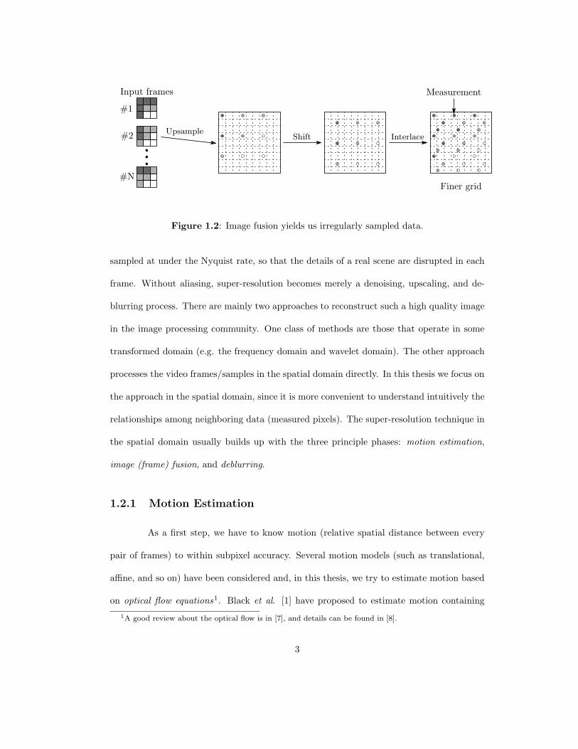
resolution grid [6]. Figure 1.2 presents a schematic representation of such super-resolution
algorithms. We note that “denoising” is a special case of the regression problem where sam-
ples at all desired pixel locations are given (illustrated in Figure 1.1(c)), but these samples
are corrupted and are to be restored. The following section gives us a brief review of the
general idea of super-resolution.
1.2 Super Resolution
The super-resolution technique reconstructs a high quality (less noise and higher
resolution) image from a noisy and low resolution video sequence. The key to super-
resolution is that the frames of a video sequence have aliasing; in other words, they are
2
UpsampleShift Interlace
#1
#2
#N
Input frames
Finer grid
Measurement
Figure 1.2: Image fusion yields us irregularly sampled data.
sampled at under the Nyquist rate, so that the details of a real scene are disrupted in each
frame. Without aliasing, super-resolution becomes merely a denoising, upscaling, and de-
blurring process. There are mainly two approaches to reconstruct such a high quality image
in the image processing community. One class of methods are those that operate in some
transformed domain (e.g. the frequency domain and wavelet domain). The other approach
processes the video frames/samples in the spatial domain directly. In this thesis we focus on
the approach in the spatial domain, since it is more convenient to understand intuitively the
relationships among neighboring data (measured pixels). The super-resolution technique in
the spatial domain usually builds up with the three principle phases: motion estimation,
image (frame) fusion, and deblurring.
1.2.1 Motion Estimation
As a first step, we have to know motion (relative spatial distance between every
pair of frames) to within subpixel accuracy. Several motion models (such as translational,
affine, and so on) have been considered and, in this thesis, we try to estimate motion based
on optical flow equations1. Black et al. [1] have proposed to estimate motion containing
1A good review about the optical flow is in [7], and details can be found in [8].
3

occlusions with the robust estimation method with which they tried to eliminate outliers.
Estimating motion to subpixel accuracy is extremely difficult; hence, Chapter 4 sums up
our approach for such accurate motion estimation. Although the performance of the optical
flow estimator is poor when the motion is large, the multiscale version of the algorithm uses
the estimator many times properly and will give us a much more accurate estimate.
1.2.2 Frame Fusion
Once the motion between the set of frames is available, we upsample all the frames
and register them to a finer grid, as illustrated in Figure 1.2. This process is often called
Shift-and-Add method [9]. Since the estimated motion are usually fractional numbers, with
the exception of the measurements from the reference frame, most pixels will not be located
on the lattice points of the finer grid. The next step we have to take is to estimate all the
high resolution pixel values from the nearby measurements, which is so-called interpolation.
There are a variety of interpolation methods in the image processing literature. Nearest
neighbor, bilinear, and cubic spline interpolation [10, 11, 12] are typical. However, they are
not designed for irregularly sampled data sets. Furthermore, the measurements are noisy
not only in their values, but also positions. The principal purpose of this thesis is to propose
suitable interpolation techniques for such irregularly sampled data.
A famous interpolation technique is the Nadaraya-Watson Estimator (NWE) [13].
NWE estimates an appropriate pixel value by taking an adaptive weighted average of sev-
eral nearby samples, and consequently its performance is totally dependent on the choice
of weights. In Chapter 3, we propose a novel method of computing the weights taking into
account not only the local density of the available samples but also the actual values of
samples. As such, the weights are automatically steered and adapted to both the given
4

sampling geometry, and the samples’ radiometry. Furthermore, due to the minimal assump-
tions made on given data sets, the method will be applicable to a wide class of problems:
efficient image upscalling, high quality reconstruction of an image from as little as 15%
of its (irregularly sampled) pixels, super-resolution from noisy and under-determined data
sets, state of the art denoising of an image corrupted by Gaussian and other noise, effective
removal of compression artifacts, demosacing, and more.
1.2.3 Deblurring
The reconstructed images are often blurry due to the blurring effects of atmosphere
and camera aperture. The purpose of this phase is to revive some high frequency compo-
nents, which visually sharpens the images. One typical choice here is the Wiener filter
[10]. This thesis will not be concerned with this phase in much depth. A simple deblurring
method is described in Appendix A.
1.3 Previous Work
A super-resolution model, which can be found in [6, 9, 14, 15], is illustrated in
Figure 1.3. In the figure, X is a continuous real scene to be estimated, Batm and Bcam
are the continuous point spread functions caused by atmospheric turbulence and camera
aperture, respectively, F is the warp operator, D is the downsampling (or discretizing)
effect, ε is measurement noise, and Y is a noisy, blurry, low resolution image (frame). Based
on the model, we can mathematically express the frame at the position [l,m] and the time
n:
Yn[l,m] =
[Bcam
n (x1, x2) ∗ ∗Fn
Batm
n (x1, x2) ∗ ∗X(x1, x2)]+ εn[l,m], (1.1)
5

noise
Real scene blur effectMotion effect
Downsampling
Frame
Batm F
Bcam
X
Y
ε
D
Atmosphere
effectblur effectCamera
Figure 1.3: A general model for multi-frame super-resolution.
where ∗∗ is the two dimensional convolution operator and ↓ is the discritizing operator. Now
we want to estimate a high resolution (discrete) unknown image X from all the measured
data Yn’s, where we define Yn and X as
Yn =
⎡⎢⎢⎢⎢⎢⎢⎢⎢⎢⎢⎣
Yn[1, 1] Yn[1, 2] · · · Yn[1,M ]
Yn[2, 1] Yn[2, 2] · · · Yn[2,M ]
......
. . ....
Yn[L, 1] Yn[L, 2] · · · Yn[L,M ]
⎤⎥⎥⎥⎥⎥⎥⎥⎥⎥⎥⎦, (1.2)
X =
⎡⎢⎢⎢⎢⎢⎢⎢⎢⎢⎢⎣
X(1, 1) X(1, 2) · · · X(1, rM)
X(2, 1) X(2, 2) · · · X(2, rM)
......
. . ....
X(rL, 1) X(rL, 2) · · · X(rL, rM)
⎤⎥⎥⎥⎥⎥⎥⎥⎥⎥⎥⎦. (1.3)
6

We call r the resolution enhancement factor. Using the notations, we can rewrite the model
(1.1) into the matrix form:
Yn = DBcamn FnBatm
n X + εn, n = 1, · · · , N, (1.4)
where the underline is the operator which makes a matrix a column stack vector, X is a
r2LM×1 vector, Batmn , Bcam
n and Fn are r2LM×r2LM matrices, D is a LM×r2LM matrix,
and Yn and εn are LM × 1 vectors. The model (1.4) can be simplified as follows. With
the two assumptions [6]: (1)spatially and temporally shift invariant point spread functions,
(2)translational motion, both Bcamn and Batm
n become symmetric constant matrices, and Fn
becomes a symmetric matrix. Since the symmetric matrices are commutable, we can rewrite
(1.4) as
Yn = DBcamFnBatmX + εn, (1.5)
= DBcamBatmFnX + εn. (1.6)
Moreover, by defining B = BcamBatm, we finally have a convenient model:
Yn = DBFnX + εn, n = 1, · · · , N. (1.7)
This is a prevalent model of super-resolution. Based on the model, an appropriate way to
estimate X is regularized least squares estimator [16], which takes the form of
XRLS = arg minX
[N∑
n=1
∥∥∥DBFnX − Yn
∥∥∥2
2+ λΥ(X)
], λ ≥ 0, (1.8)
where Υ(·) is the regularization function (see Table A.1 in Appendix A), and λ is a regular-
ization parameter (a positive number) which enables us to control how strongly we consider
the regularization term. Using the estimator, an example is demonstrated in the following.
Figure 1.4 shows Tank sequence (64 × 64, 8 frames) which is a real sequence taken by an
7

frame1
20 40 60
20
40
60
frame2
20 40 60
20
40
60
frame3
20 40 60
20
40
60
frame4
20 40 60
20
40
60
frame5
20 40 60
20
40
60
frame6
20 40 60
20
40
60
frame7
20 40 60
20
40
60
frame8
20 40 60
20
40
60
Figure 1.4: Tank sequence.
infrared camera, courtesy of B. Yasuda and the FLIR research groupe in the Sensors Tech-
nology Branch, Wright Laboratory, WPAFB, OH. A reconstructed high resolution image2
is shown in Figure 1.5. We can see the more details with the estimated image such as the
wheels of the truck which are impossible for us to realize in each low resolution frame.
This section showed that a prevalent super-resolution method. In Chapter 2, we
will present a different super-resolution approach, and show an example on Tank sequence.
In Chapter 5, we will demonstrate further real super-resolution examples with the different
super-resolution approach by combining motion estimation in Chapter 4, image fusion in
Chapter 2 and its extension in Chapter 3, and image deblurring in Appendix A.2This image provided by a software coded by S. Farsiu [6], which is available online at
www.cse.ucsc.edu/∼milanfar/SR-Software.htm
8

50 100 150 200 250 300
50
100
150
200
250
300
Figure 1.5: An example of the estimated image from Tank sequence.
1.4 Summary
We briefly reviewed image reconstruction from irregularly sampled data sets with
existing algorithms in this introductory chapter. However, most of these algorithms are
designed for a specific model, and consequently they cannot be applicable for other prob-
lems. If only one method can do denoising and interpolation simultaneously with a superior
performance, we will be relieved from choosing the best algorithm for a specific problem.
The main purpose of this thesis is to present such a universal algorithm.
Contributions of this thesis are the following: (1) we describe and propose kernel
9

regression as an effective tool for both denoising and interpolating images, and establish
its relation with some popular existing techniques, (2) we propose a novel adaptive gener-
alization of kernel regression with superior results in both denoising and interpolation (for
single or multi-frame) applications. This thesis is structured as follows. In Chapter 2, the
kernel regression framework will be described as an effective tool for image processing with
its fundamental property, the relationships with some other famous methods, and a simple
example on Tank sequence. In Chapter 3, the data-adapted (non-linear) version of kernel
regression will be presented. In Chapter 4, we sum up the accurate motion estimation al-
gorithm in order to fuse images. In Chapter 5, many demonstrations on a wide class of
problems will be shown, and conclude this thesis. In Chapter 6, the installation and manu-
als of the program codes, which produce the results shown in Chapter 5, will be explained.
Finally, in Chapter 7, we indicate some of our future directions on this research.
10

Chapter 2
Kernel Regression
2.1 Introduction
In this chapter, we make contact with the field of non-parametric statistics and
present a development and generalization of tools and results for use in image processing
and reconstruction. Furthermore, we establish key relationships with some popular existing
methods and show how several of these algorithms are special cases of the framework.
2.2 Kernel Regression for Univariate Data
Classical parametric denoising methods rely on a specific model of the signal of in-
terest, and seek to compute the parameters of this model in the presence of noise. Examples
of this approach are represented in diverse problems ranging from denoising to upscaling
and interpolation. A generative model based upon the estimated parameters is then pro-
duced as the best estimate of the underlying signal. Some representative examples of the
11

parametrization are quadratic, periodic, and monotone models [17],
yi = β0 + β1xi + β2x2i + εi, yi = β0 sin (β1xi) + εi, yi =
β0
β1 + xi+ εi, i = 1, 2, · · · , P,
(2.1)
where yi’s are the measurements, xi’s are the coordinates (positions), P is the number of the
measured samples, εi’s are independent and identically distributed zero mean noise value,
and βn are the model parameters to be estimated. Least square approach1 [16] is usually
employed to estimate the unknown model parameters. For example, in the quadratic case,
the unknown parameters are estimated as
minβn
P∑i=1
[yi − β0 − β1xi − β2x
2i
]2. (2.2)
Unfortunately, as natural images rarely follow such fixed models, the quality of reconstructed
images is often not satisfactory.
In contrast to the parametric methods, non-parametric methods rely on the data
itself to dictate the structure of the model, in which case this implicit model is referred
to as a regression function [17]. With the relatively recent emergence of machine learning
methods, kernel methods have become well-known and used frequently for pattern detection
and discrimination problems [19], and estimation of real-valued functions by the support
vector method in Chapter 11 and 13 of [20]. Surprisingly, it appears that the corresponding
ideas in estimation - what we call here kernel regression, are not widely known or used in the
image and video processing literature. Indeed, in the last decade, several concepts related
to the general theory this thesis promotes here have been rediscovered in different guises,
and presented under different names such as normalized convolution [21, 22], the bilateral
filter [23] (the latter having been carefully investigated mathematically in [24]), mean-shift
1Total least square approach [18] is a more appropriate choice when the coordinates xi’s are also noisy.A super-resolution algorithm using kernel regression, which we will present later in this chapter, is the case.
12

[25], edge directed interpolation [26], and moving least squares [27]. Later in this thesis,
some of these concepts and their relation to the general regression theory will be discussed.
To simplify the presentation, let us first treat the univariate data case where the measured
data are given by
yi = z(xi) + εi, i = 1, 2, · · · , P, (2.3)
where z(·) is the (hitherto unspecified) regression function and εi’s are the independent
and identically distributed zero mean noise values (with otherwise no particular statistical
distribution assumed). As such, kernel regression provides a rich mechanism for computing
point-wise estimates of the function with minimal assumptions on the signal model.
While the particular form of z(·) may remain unspecified, if we assume that it is
locally smooth to some order N , then to estimate the value of the function at any point x
given the data, we can rely on a generic local expansion of the function about this point.
Specifically, if x is near the sample at xi, we have the N -term Taylor series2
z(xi) ≈ z(x) + z′(x)(xi − x) +12!
z′′(x)(xi − x)2 + · · · + 1N !
z(N)(x)(xi − x)N (2.4)
= β0 + β1(xi − x) + β2(xi − x)2 + · · · + βN (xi − x)N . (2.5)
The above suggests that if we now think of the Taylor series as a local representation of the
regression function, estimating the parameter β0 yields the desired (local) estimate of the
regression function based on the data. Indeed, the other parameters βnNn=1 will provide
localized information on the n-th derivatives of the regression function. Naturally, since
this approach is based on local approximations, a logical step to take is to estimate the
parameters βnNn=0 from the data while giving the nearby samples higher weight than
samples farther away. A weighted least-square formulation [16] capturing this idea is to
2Other expansions are also possible, e.g. orthogonal series.
13

solve the following optimization problem:
minβnN
n=0
P∑i=1
[yi − β0 − β1(xi − x) − β2(xi − x)2 − · · · − βN (xi − x)N
]2 1h
K
(xi − x
h
),
(2.6)
where K(·) is the kernel function (weight function) [17] which penalizes distance away from
the local position where the approximation is centered, and the smoothing parameter h (also
called the bandwidth) controls the strength of this penalty. In particular, the function K(·)
is a symmetric function which attains its maximum at zero, satisfying
∫R1
tK(t)dt = 0,
∫R1
t2K(t)dt = c, (2.7)
where c is a some constant value. The choice of the particular form of the function K(·) is
open, and may be selected as a Gaussian, exponential, or other forms which comply with
the above constraints (some popular choice of K(·) are shown in Table 2.1). Experimental
studies such as in [28] show that the choice of the kernel has an insignificant effect on the
accuracy of estimation and therefore the preference is given to the differentiable kernels with
low computational complexity such as the Gaussian kernel.
Several important point are worth making here. First, the above structure allows
for tailoring the estimation problem to the local characteristics of the data, whereas the
standard parametric model is intended as a more global fit. Second, in the estimation of
the local structure, higher weight is given to the nearby data as compared to samples that
are farther away from the center of the analysis window. Meanwhile, this approach does
not specifically require that the data follow a regular or periodic sampling structure. More
specifically, so long as the samples are near the point x, the non-parametric framework (2.6)
is valid. Again this is in contrast to the general parametric approach (e.g. (2.2)) which
generally either does not directly take the location of the data samples into account, or
14

Epanechnikov:
−1.5 −1 −0.5 0 0.5 1 1.5
0
0.2
0.4
0.6
0.8
1
K(t) =
34(1 − t2) for |t| < 1
0 otherwise
Biweight:
−1.5 −1 −0.5 0 0.5 1 1.5
0
0.2
0.4
0.6
0.8
1
K(t) =
1516
(1 − t2)2 for |t| < 1
0 otherwise
Triangle:
−1.5 −1 −0.5 0 0.5 1 1.5
0
0.2
0.4
0.6
0.8
1
K(t) =
1 − |t| for |t| < 10 otherwise
Laplacian:
−4 −3 −2 −1 0 1 2 3 4−0.1
0
0.1
0.2
0.3
0.4
0.5
K(t) =12
exp (−|t|)
Gaussian:
−4 −3 −2 −1 0 1 2 3 4−0.1
0
0.1
0.2
0.3
0.4
K(t) =1√2π
exp(−1
2t2)
Table 2.1: Popular choices for the kernel function.
relies on regular sampling over a grid. Third, and no less important, the proposed approach
is useful for both denoising, and equally viable for interpolation of sampled data at points
where no actual samples exist. Given the above observations, the kernel-based methods
appear to be well-studied for a wide class of image processing problems of practical interest.
Returning to the estimation problem based upon (2.6), one can choose the order
N to effect an increasingly more complex local approximation of the signal. In the non-
parametric statistics literature, locally constant, locally linear, and locally quadratic approx-
imations (corresponding to N = 0, 1, 2) have been considered most widely [17, 29, 30, 31].
In particular, choosing N = 0, a locally adaptive linear filter is obtained, which is known
15

as the Nadaraya-Watson Estimator (NWE) [13]. Specifically, this estimator has the form
z(x) =
P∑i=1
Kh(xi − x) yi
P∑i=1
Kh(xi − x)
, Kh(t) =1h
K
(t
h
). (2.8)
When all the data yi’s are uniformly distributed as shown in Figure 1.1(c), the NWE is
nothing but a simple convolution that has been practiced for 100 years in signal processing.
As described earlier, the NWE is the simplest manifestation of an adaptive filter
resulting from the kernel regression framework. As we shall see later in Section 3.2.1, the
bilateral filter [23, 24] can be interpreted as a generalization of the NWE with a modified
kernel definition.
Of course, higher order approximations (N > 0) are also possible. Note that
the choice of the order in parallel with the smoothness h affect the bias and variance of
estimation. Mathematical expression for bias and variance can be found in [32, 33], and
therefore here we briefly review their properties. In general, lower order approximates such
as NWE (N = 0), result in smoother images (large bias and small variance) as there are not
enough degree of freedom. On the contrary, over-fitting happens in regression using higher
orders of approximation, resulting in small bias and large estimation variance. We also note
that smaller values for h result in small bias and consequently large variance in estimates.
Optimal order and smoothing parameter selection procedures are studied in [27].
The performance of kernel regressors of different orders is compared in the illus-
trative examples of Figure 2.1. In the first experiment, illustrated in the first row, a set of
moderately noisy (variance of the additive Gaussian noise is 0.1) equally-spaced samples of
a function are used to estimate the underlying function. As expected, the computationally
more complex high order interpolation (N = 2) results in a better estimate than the lower
16

ordered interpolators (N = 0 or 1). The presented quantitative comparison of RMSE3 sup-
ports this claim. The second experiment, illustrated in the second row, shows that for the
heavily noisy data sets (variance of the additive Gaussian noise is 0.5), the performance of
lower ordered regressors is better. Note that the performance of the N = 0 and N = 1
ordered estimators for these equally-spaced sampled experiments are identical. In Section
2.3.2, we study this property in more detail.
2.2.1 Related Regression Methods
In addition to kernel regression methods, which this thesis is advocating, there
are several other effective regression methods such as B-spline interpolation [11], orthogonal
series [34, 30], cubic spline interpolation [12] and spline smoother [30, 11, 35]. We briefly
review these methods and see how they are related in this section.
Following the notation used in the previous subsection, the B-spline interpolation
is expressed as the linear combination of shifted spline functions
z(x) =∑
k
βkBq(x − k), (2.9)
where the qth order B-spline function is defined as a q + 1 times convolution of the zero-th
order B-spline function [11],
Bq(x) = B0(x) ∗ B0(x) ∗ · · · ∗ B0(x)︸ ︷︷ ︸q+1
, where B0(x) =
⎧⎪⎪⎪⎪⎪⎪⎨⎪⎪⎪⎪⎪⎪⎩1, − 1
2 < x < 12
12 , |x| = 1
2
0, else
. (2.10)
The scalar k in (2.9), often referred to as the knot, defines the center of a spline. The least
squares formulation [16] is usually exploited to estimate the B-spline coefficients βk.3Root Mean Square Error of an estimate is defined as RMSE =
pE(z(x) − z(x))2, where E is the
expected value operator.
17

−2 0 2 4 6 8
0
0.5
1
1.5
x
z(x)
−2 0 2 4 6 8
0
0.5
1
1.5
x
z(x)
−2 0 2 4 6 8
0
0.5
1
1.5
xz(
x)
−2 0 2 4 6 8
0
0.5
1
1.5Local Constant Estimator (N=0)
x
z(x)
Actual functionEstimated functionData
−2 0 2 4 6 8
0
0.5
1
1.5Local Linear Estimator (N=1)
x
z(x)
−2 0 2 4 6 8
0
0.5
1
1.5Local Quadratic Estimator (N=2)
x
z(x)
Figure 2.1: Examples of local polynomial regression of an equally-spaced data set. Thesignals in the first and second rows are contaminated with the Gaussian noise of var(εi) =0.1 and 0.5, respectively. The dashed, solid lines, and dots represent the actual function,estimated function, and the noisy data, respectively. The columns from left to right showthe constant, linear, and quadratic interpolation results. Corresponding RMSE’s for the firstrow experiments are 0.0025, 0.0025, 0.0009 and for the second row are as 0.0172, 0.0172,0.0201.
The B-spline interpolation method bears some similarities to the kernel regression
method. One major difference between these method is in the number and position of the
knots as illustrated in Figure 2.2. While in the classical B-spline method the knots are
located in equally spaced positions, in the case of kernel regression the knots are implicitly
located on the sample positions. A related method, the Non-Uniform Rational B-Spline
(NURBS) is also proposed in [36] to address this shortcoming of the classical B-spline
method, by irregularly positioning the knots with respect to the underlying signal.
18

x
Regression function
Measurements Bumps
(a) Kernel regression
x
Knots
(b) B-splineFigure 2.2: A comparison of the position of knots in (a) Kernel regression and (b) classicalB-Spline methods.
Cubic spline interpolation technique is one of the most popular members of the
spline interpolation family which is based on fitting a polynomial between any pair of con-
secutive data. Assuming that the second derivative of the regression function exists, cubic
spline interpolation is defined as
z(x) = β0(i) + β1(i)(xi − x) + β2(i)(xi − x)2 + β3(i)(xi − x)3, x ∈ [xi, xi+1] , (2.11)
where under the following boundary conditions
z(x)∣∣∣x−
i
= z(x)∣∣∣x+
i
, z′(x)∣∣∣x−
i
= z′(x)∣∣∣x+
i
, z′′(x)∣∣∣x−
i
= z′′(x)∣∣∣x+
i
,
z′′(x1) = z′′(xP ) = 0, (2.12)
all the coefficients Bi’s can be uniquely defined [12].
Note that an estimated curve by cubic spline interpolation passes through all data
points which is ideal for the noiseless data case. However, in most practical applications,
data are contaminated with noise and therefore such perfect fits are no longer desirable.
Consequently a related method called spline smoother is proposed. In spline smoother the
above hard conditions are replaced with soft ones, by introducing them as Bayesian priors
which penalize rather than constrain non-smoothness in the interpolated images. A popular
19

implementation of the spline smoother [11] is given by
z(x) = arg minz(x)
[P∑
i=1
yi − z(xi)2 + λ‖z′′‖22
], ‖z′′‖2
2 =∫
z′′(x)2dx, (2.13)
where z(xi) can be replaced by either (2.9) or any orthogonal series4, and λ is the regulariza-
tion parameter. Note that assuming a continuous sample density function, the solution to
this minimization problem is equivalent to the NWE (2.8) with the following kernel function
and a variable smoothing parameter h
K(t) =12
exp(− |t|√
2
)sin
( |t|√2
+π
4
), h(xi) =
(λ
Pf(xi)
) 14
, (2.14)
where f(·) is the density of samples [30, 38]. In Chapter 5, performance comparisons with
data-adapted kernel regression (q.v. Chapter 3) will be presented.
2.3 Kernel Regression for Bivariate Data and its Prop-
erties
This section introduces the formulation of the classical kernel regression method
for bivariate data and establishes its relation with the linear filtering idea. Some intuitions
on computational efficiency will be also provided as well as weakness of this method, which
motivate the development of more powerful regression tools in the next chapter.
2.3.1 Kernel Regression Formulation
Similar to the univariate data case in (2.3), the model of bivariate data (e.g. the
samples in Figure 1.1(b)) is given by
yi = z(xi) + εi, xi = [x1i, x2i]T , i = 1, 2, · · · , P, (2.15)4A successful implementation based on this method for image reconstruction has done by Arigovindan
et al. [37].
20

where the coordinates of the measured data yi is now the 2× 1 vector xi. Correspondingly,
the local expansion of the regression function is given by
z(xi) ≈ z(x) + ∇z(x)T (xi − x) +12!
(xi − x)THz(x) (xi − x) + · · ·
= z(x) + ∇z(x)T (xi − x) +12vecTHz(x) vec
(xi − x)(xi − x)T
+ · · · ,
(2.16)
where ∇ and H are the gradient and Hessian operators, respectively and vec(·) is the
vectorization operator [32], which lexicographically orders a matrix into a vector. Defining
vech(·) as the half-vectorization operator [32] of the lower-triangular portion of the matrix,
e.g.,
vech
⎛⎜⎜⎝⎡⎢⎢⎣ a11 a12
a21 a22
⎤⎥⎥⎦⎞⎟⎟⎠ = [a11 a21 a22]
T, (2.17)
vech
⎛⎜⎜⎜⎜⎜⎜⎝
⎡⎢⎢⎢⎢⎢⎢⎣a11 a12 a13
a21 a22 a23
a31 a32 a33
⎤⎥⎥⎥⎥⎥⎥⎦
⎞⎟⎟⎟⎟⎟⎟⎠ = [a11 a21 a31 a23 a32 a33]T
, (2.18)
and considering the symmetry of the Hessian matrix, (2.16) simplifies to
z(xi) = β0 + βT1 (xi − x) + βT
2 vech(xi − x)(xi − x)T
+ · · · . (2.19)
Then, comparison between (2.16) and (2.19) suggests that β0 = z(x) is the pixel value of
interest and the vectors β1 and β2 are
β1 =
[∂z(x)∂x1
∣∣∣∣x=xi
∂z(x)∂x2
∣∣∣∣x=xi
]T
, (2.20)
β2 =12
[∂2z(x)∂x2
1
∣∣∣∣x=xi
2∂2z(x)∂x1∂x2
∣∣∣∣x=xi
∂2z(x)∂x2
2
∣∣∣∣x=xi
]T
. (2.21)
21

As in the case of univariate data, the βn are computed from the following optimization
problem:
minβnN
n=0
P∑i=1
[yi − β0 − βT
1 (xi − x)T − βT2 vech
(xi − x)(xi − x)T
− · · ·]2
KH(xi − x),
(2.22)
with
KH(t) =1
det (H)K(H−1t
), (2.23)
where K(·) is the 2-D realization of the kernel function illustrated in Table 2.1, and H is
the 2 × 2 smoothing matrix, which will be studied more carefully later in this chapter. It
is also possible to express (2.22) in a matrix form as a weighted lease squares optimization
problem [16, 27],
arg minb
‖y − Xxb‖2Wx
= arg minb
(y − Xxb)T Wx (y − Xxb) , (2.24)
where
y = [y1 y2 · · · yP ]T , b =[β0 βT
1 βT2 · · ·
]T
, (2.25)
Wx = diag [KH(x1 − x), KH(x2 − x), · · · , KH(xP − x)] , (2.26)
Xx =
⎡⎢⎢⎢⎢⎢⎢⎢⎢⎢⎢⎣
1 (x1 − x)T vechT(x1 − x)(x1 − x)T
· · ·
1 (x2 − x)T vechT(x2 − x)(x2 − x)T
· · ·...
......
...
1 (xP − x)T vechT(xP − x)(xP − x)T
· · ·
⎤⎥⎥⎥⎥⎥⎥⎥⎥⎥⎥⎦, (2.27)
with “diag” defining the diagonal elements of a diagonal matrix.
Regardless of the regression order (N), as our primary interest is to compute an
estimate of the image (pixel values), the necessary computations are limited to the ones that
estimate the parameter β0. Therefore the weighted least squares estimation is simplified to
z(x) = β0 = eT1
(XT
xWxXx
)−1XT
xWx y, (2.28)
22

where e1 is a column vector (the same size of b in (2.25)) with the first element equal
to 1, and the rest equal to zero. Of course, there is a fundamental difference between
computing β0 for the N = 0 case, and using a high order estimator (N > 0) and then
effectively discarding direct calculation of all βn except β0. Unlike the former case, the
latter method computes estimates of pixel values assuming a N th order locally polynomial
structure is present.
2.3.2 Equivalent Kernel
In this subsection we derive a computationally more efficient and intuitive solution
to the classic kernel regression problem. Study of (2.28) shows that XTxWxXx is a (N +
1) × (N + 1) block matrix, with the following structure:
XTxWxXx =
⎡⎢⎢⎢⎢⎢⎢⎢⎢⎢⎢⎣
s11 s12 s13 · · ·
s21 s22 s23 · · ·
s31 s32 s33 · · ·...
......
. . .
⎤⎥⎥⎥⎥⎥⎥⎥⎥⎥⎥⎦, (2.29)
where slm is an l×m matrix (a block). The block elements of (2.29) for the orders of up to
N = 2 are as follows:
s11 =P∑
i=1
KH(xi − x) (2.30)
s12 = sT21 =
P∑i=1
(xi − x)T KH(xi − x) (2.31)
s22 =P∑
i=1
(xi − x)(xi − x)T KH(xi − x) (2.32)
23

s13 = sT31 =
P∑i=1
vechT(xi − x)(xi − x)T
KH(xi − x) (2.33)
s23 = sT32 =
P∑i=1
(xi − x)vechT(xi − x)(xi − x)T
KH(xi − x) (2.34)
s33 =P∑
i=1
vech(xi − x)(xi − x)T
vechT
(xi − x)(xi − x)T
KH(xi − x). (2.35)
Considering the above shorthand notation, (2.28) can be represented as a local linear filtering
process:
z(x) =P∑
i=1
Wi(x;N,H) yi, (2.36)
where
Wi(x; 0,H) =KH(xi − x)
s11(2.37)
Wi(x; 1,H) =
1 − s12s−1
22 (xi − x)
KH(xi − x)
s11 − s12s−122 s21
(2.38)
Wi(x; 2,H) =
[1 − S12S−1
22 (xi − x) − S13S−133 vech
(xi − x)(xi − x)T
]KH(xi − x)
s11 − S12S−122 s21 − S13S−1
33 s31
.
(2.39)
and
S12 = s12 − s13s−133 s32, S22 = s22 − s23s−1
33 s32,
S13 = s13 − s12s−122 s23, S33 = s33 − s32s−1
22 s23. (2.40)
Therefore, regardless of the order, the classical kernel regression is nothing but local weighted
averaging of data (linear filtering), where the order determines the type and complexity
of the weighting scheme. This also suggest that the high order regressions (N > 0) are
equivalents of the zero-th order regression (N = 0) with a more complex kernel function. In
other words, to effect the higher order regressions, the original kernel KH(xi−x) is modified
to yield a newly adapted equivalent kernel [33].
24

−10 0 10
−15
−10
−5
0
5
10
15
Sample distribution
x1
x 2
−15 −10 −5 0 5 10 15
0
0.05
0.1
0.15
0.2
0.25
Equivalent kernel
x1
W
N=2
N=0,1
(a) (b)
Figure 2.3: (a) A uniformly sampled data set. (b) A horizontal slice of the equivalentkernels of orders N =0 , 1, and 2 for the regularly sampled data in (a). The kernel KH in(2.22) is modeled as a Gaussian, with the smoothing matrix H = Diag[10, 10].
To have a better intuition of equivalent kernels, we study the example in Figure
2.3, which illustrates a uniformly sampled data set and the horizontal slices of its corre-
sponding equivalent kernels for the regression orders N = 0, 1 and 2. The direct result of the
symmetry condition (2.7) on KH(xi −x) with uniformly sampled data is that all odd-order
moments (s2j,2k+1 and s2k+1,2j)’s consist of elements with values very close to zero. As this
observation holds for all regression orders, for the regularly sampled data, the N = 2q − 1
order regression is preferred to the computationally more complex N = 2q order regression,
as they produce almost identical results. This property manifests itself in Figure 2.3, where
the N = 0 or 1 ordered equivalent kernels are identical.
This example also shows that unlike the N = 0, 1 cases in which the equivalent
kernel only consists of positive values, the second order equivalent kernel has both positive
and negative elements. Therefore, when we look at the response of equivalent kernel in the
25

frequency domain, the second order equivalent kernel has a clearer cutoff between passed
and filtered frequencies than the zero-th or first order equivalent kernel. The response of
the second order one is very similar to the second order Butterworth low-pass filter.
In the next experiment, we compare the equivalent kernels for an irregularly sam-
pled data set shown in Figure 2.4(a). The second order equivalent kernel for the sample
marked with “×”, is shown in Figure 2.4(b). Figure 2.4(c) and Figure 2.4(d) show the
horizontal and vertical slices of this kernel, respectively. This figure demonstrates the fact
that the equivalent kernels tend to adapt themselves to the density of available samples.
Also, unlike the regularly sampled data case, since the odd-order moments are not equal to
zero, the N = 0 and N = 1 equivalent kernels are no longer identical.
2.3.3 The Selection of Smoothing Matrices
The spread of the kernel as defined in (2.23), and consequently the performance of
the estimator, depend on the choice of the smoothing matrix H [32]. For the bivariate data
cases, the smoothing matrix is a 2× 2 positive definite matrix which is generally defined for
each measured sample as
Hi =
⎡⎢⎢⎣ h1i h2i
h3i h4i
⎤⎥⎥⎦ , (2.41)
where Hi extends the kernel5 to contain a sufficient number of samples. As illustrated in
Figure 2.5, it is reasonable to use smaller kernels in the areas with more available samples,
and likewise larger footprint is more suitable for the more sparsely sampled regions of the
image.
The cross validation (leave-one-out) method [17, 30] is a popular method for es-
5The kernel is often called the mercer kernel, which measures similarity between data, in vast literatureon kernel based regression in multidimensional machine learning, and the way to define the smoothing matrixHi by (2.41) is a more general version of the mercer kernels.
26

−10 0 10
−15
−10
−5
0
5
10
15
Sample distribution
x1
x 2
−15−10
−50
510
15
−15−10
−50
510
15−0.05
0
0.05
0.1
0.15
0.2
x1
Equivalent kernel, N=2
x2
W
−15 −10 −5 0 5 10 15
0
0.05
0.1
0.15
0.2
0.25
Equivalent kernel
x1
W
−15 −10 −5 0 5 10 15
0
0.05
0.1
0.15
0.2
0.25
Equivalent kernel
x2
W
N=2
N=1
N=0
N=2
N=1
N=0
(a) (b)
(c) (d)
Figure 2.4: Equivalent kernels for an irregularly sampled data set are shown in (a). (b)is the second order (N = 2) equivalent kernel. The horizontal and vertical slices of theequivalent kernels of different orders (N = 0, 1, 2) are compared in (c) and (d), respectively.In this example, the kernel KH in (2.22) was modeled as a Gaussian, with the smoothingmatrix H = Diag[10, 10].
timating the elements of the local Hi’s. However, as the cross validation method is com-
putationally very expensive, we usually use a simplified and computationally more efficient
27

small footprintlarge footprint
Figure 2.5: Smoothing (kernel size) selection by sample density.
model of the smoothing matrices as
Hi = hµiI, (2.42)
where µi is a scalar that captures the local density of the data samples and h is the global
smoothing parameter.
The global smoothing parameter is directly computed from the cross validation
method, by minimizing the following cost function
ζcv(h) =P∑
i=1
zh,−i(xi) − yi2, (2.43)
where zh,−i(xi) is the estimated pixel values without the ith sample with the global smoothing
parameter h. As ζcv might not be differentiable, we use the Nelder-Mead optimization
algorithm [39] to estimate h. To further reduce the computations, rather than leaving a
single sample out, it is possible to leave out a set of samples (a hole row and column).
Following [28], the local density parameter µi is estimated as follows
µi =(
f(xi)g
)−α
, (2.44)
28
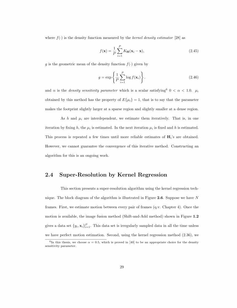
where f(·) is the density function measured by the kernel density estimator [28] as
f(x) =1P
P∑i=1
KH(xi − x), (2.45)
g is the geometric mean of the density function f(·) given by
g = exp
1P
P∑i=1
log f(xi)
. (2.46)
and α is the density sensitivity parameter which is a scalar satisfying6 0 < α < 1.0. µi
obtained by this method has the property of Eµi = 1, that is to say that the parameter
makes the footprint slightly larger at a sparse region and slightly smaller at a dense region.
As h and µi are interdependent, we estimate them iteratively. That is, in one
iteration by fixing h, the µi is estimated. In the next iteration µi is fixed and h is estimated.
This process is repeated a few times until more reliable estimates of Hi’s are obtained.
However, we cannot guarantee the convergence of this iterative method. Constructing an
algorithm for this is an ongoing work.
2.4 Super-Resolution by Kernel Regression
This section presents a super-resolution algorithm using the kernel regression tech-
nique. The block diagram of the algorithm is illustrated in Figure 2.6. Suppose we have N
frames. First, we estimate motion between every pair of frames (q.v. Chapter 4). Once the
motion is available, the image fusion method (Shift-and-Add method) shown in Figure 1.2
gives a data set yi,xiPi=1. This data set is irregularly sampled data in all the time unless
we have perfect motion estimation. Second, using the kernel regression method (2.36), we
6In this thesis, we choose α = 0.5, which is proved in [40] to be an appropriate choice for the densitysensitivity parameter.
29

#1
#2
#N
Input frames
Motion Shift-and-Add
KernelDeblurringX
yi,xiPi=1
Z
methodestimation
regression
Figure 2.6: The block diagram of the super-resolution algorithm using kernel regression.
estimate the high resolution image Z, which is defined as
Z =
⎡⎢⎢⎢⎢⎢⎢⎢⎢⎢⎢⎣
z(1, 1) z(1, 2) · · · z(1, rM)
z(2, 1) z(2, 2) · · · z(2, rM)
......
. . ....
z(rL, 1) z(rL, 2) · · · z(rL, rM)
⎤⎥⎥⎥⎥⎥⎥⎥⎥⎥⎥⎦. (2.47)
However the estimated image Z is often blurry due to the blur effects caused by atmospheric
turbulence and camera aperture. Hence, third, we need to deblur it by using (A.2) in
Appendix A in order to obtain the sharper image X.
In Figure 2.7, an simple example on Tank sequence shown in Figure 1.4 is illus-
trated with the algorithm just stated above. Figures 2.7(a), (b), and (c) are showing the
estimated images by (2.36) with the regression order N = 0, 1, and 2, respectively. The same
global smoothing parameter, h = 0.8, was used for each case. We can see the significant
improvements between the regression order 0 and 1, since equivalent kernels are different
in the case of irregularly sampled data (see Figure 2.4). With the second order (N = 2),
30

we have an even better image (Figure 2.7(c)). Using the deblurring technique described in
Appendix A (5 × 5 Gaussian blur kernel with variance 1.0, the regularization term of 5× 5
bilateral total variation, the regularization parameter λ = 0.2 and α = 0.5 are used with 50
iterations), the final output is shown in Figure 2.7(d), as applied on the image in Figure
2.7(c).
2.5 Summary
In this chapter we reviewed the classical kernel regression framework, and showed
that it can be regarded as a locally adaptive linear filtering process and an example of image
reconstruction on the tank sequence. The tank sequence has relatively little noise and no
compression artifacts, hence the reconstructed image are quite good. However a real video
sequence could have more noise and compression artifacts. In order to produce a superior
quality output from such a severe case, in the next chapter, we propose and study the
adaptive kernel regression methods with locally non-linear filtering properties.
31

(a) N = 0 (b) N = 1
(c) N = 2 (d) The reconstructed image
Figure 2.7: A super-resolution example on the tank sequence.
32

Chapter 3
Data-Adapted Kernel Regression
3.1 Introduction
In the previous chapter, we studied the kernel regression method, its properties, and
showed its usefulness for image restoration and reconstruction purpose. One fundamental
improvement on the above method can be realized by noting that, the local polynomial kernel
regression estimates, independent of the order (N), are always local linear combinations
(weighted averages) of the data. As such, though elegant, relatively easy to analyze, and
with attractive asymptotic properties [32], they suffer from an inherent limitation due to
this local linear action on the data. In what follows, we discuss extensions of the kernel
regression method that enable this structure to have nonlinear, more effective, action on the
data.
A strong denoising effect and interpolating all the pixels from a very sparse data
set can be realized by making the global smoothing parameter (h) larger. However, with
such a larger h, the estimated image will be more blurred so that we have sacrificed details.
33

edgeedge
(a) (b)
Figure 3.1: Kernel spread in a uniformly sampled data set. (a) Kernels in the classicmethod depend only on the sample density. (b) Data-adapted kernels elongate with respectto the edge.
In order to have both a strong denoising/interpolating effect and a sharper image, one can
consider an alternative approach that will adapt the local effect of the filter using not only
the position of the nearby samples, but also their gray values. That is to say, the proposed
kernels will take into account two factors: spatial distances and radiometric (gray value)
distances. With this idea, this chapter presents a novel non-linear filter algorithm called
data-adapted (or steered) kernel regression.
3.2 Data-Adapted Kernel Regression
Data-adapted kernel regression methods rely not only on the sample density, but
also on the benefits of edge artifacts from the radiometric properties of these samples.
Therefore, the effective size and spread of the kernel is locally adapted to the structure of
objects on an image. This property is illustrated in Figure 3.1, where the classical kernel
spreads and the adaptive kernel spreads in presence of an edge are compared.
On the data-adapted kernel regression approach, in order to take into account the
structure information of a data set, we can simply add one more concept to the kernel
34

function as a parameter. The optimization problem arises here as follows:
minβnN
n=0
P∑i=1
[yi − β0 − βT
1 (xi − x)T − βT2 vech
(xi − x)(xi − x)T
− · · ·]2
K(xi −x, yi − y),
(3.1)
where the data-adapted kernel function K now depends on the spatial differences (xi − x)
as well as the local radiometric differences (yi − y). The rest of this chapter presents the
selections of the adapted kernel (K).
3.2.1 Bilateral Kernel Regression
A simple and intuitive choice of the K is to use separate terms for penalizing the
spatial differences between the position of interest x and its nearby position xi, and the
radiometric differences between the corresponding pixel value y and yi:
K(xi − x, yi − y) ≡ KHs(xi − x)Khr (yi − y), (3.2)
where Hs is the spatial smoothing matrix defined as Hs = hsI, and hs and hr are the
spatial and radiometric smoothing parameters. We call this the bilateral kernel. However,
the kernel has a weakness in that the radiometric value y at an arbitrary position x is not
available occasionally as is the case for interpolation problems. Hence we cannot compute
the radiometric weight Khr (yi − y) directly. We may still use the radiometric kernel, but in
such cases a pilot estimate will be needed first to estimate the y. When, in general, y at a
arbitrary position x does exist, the optimization problem with the kernel can be rewritten
as:
minβnN
n=0
P∑i=1
[yi − β0 − βT
1 (xi − xj)T − βT2 vech
(xi − xj)(xi − xj)T
− · · ·]2
·KHs(xi − xj)Khr (yi − yj),
(3.3)
35

which we call Bilateral Kernel Regression. Note that the regression now lost the interpolation
ability. This can be better understood by studying the spacial case of N = 0, which results
in a data-adapted version of the Nadaraya-Watson [13] estimator:
z(xi) =
P∑i=1
KHs(xi − xj)Khr (yi − yj) yi
P∑i=1
KHs(xi − xj)Khr (yi − yj)
. (3.4)
Interestingly, this is nothing but the recently well-studied and popular bilateral filter [23, 24],
both of whose kernels were chosen as Gaussian. In our framework, it is not required for
us to pick the same kernel for both spatial and radiometric kernels. Of course, the higher
order regressions (N > 0) are also available and they can have better performance than
the bilateral filter (the zero-th order bilateral kernel regression (3.4)). As described above,
we cannot apply this regression directly to interpolation problems, and the direct solution
of (3.3) is limited to the denoising problem. Later in this chapter, this limitation can be
overcome by using an initial estimate of y in an iterative set-up.
In any event, breaking K into the spatial and radiometric kernels as utilized in
the bilateral case weakens the estimation performance. A simple justification for this claim
comes from studying the very noisy data sets, where the radiometric differences (yi − yj)’s
tend to be large and as a result all radiometric weights are very close to zero, and effectively
useless. Buades et al. gave this discussion in [41], and they proposed the non-local means
algorithm to enhance denoising effect. However, the algorithm has also a limited scope
of use: image denoising. The following subsection provides a solution to overcome this
drawback of the bilateral kernel approach and the limited scope of use.
36

3.2.2 Steering Kernel Regression
The filtering procedure we proposed above takes the idea of the bilateral kernel one
step further, based upon the earlier kernel regression framework. In particular, we observe
that the effect of computing Khr (yi − y) in (3.2) is to implicitly measure a function of the
local gradient estimated between neighboring pixel values, and to use this estimate to weigh
the respective measurements. As an example, if a pixel is located near an edge, then pixels
on the same side of the edge will have much stronger influence in the filtering. With this
intuition in mind, we propose a two-step approach where first an initial analysis of the image
local structure is carried out. In a second stage, this structure information is then used to
adaptively “steer” the local kernel, resulting in elongated, elliptical contours spread along
the directions of the local edge structure. With these locally adapted kernels, the image
restoration and reconstruction are effected most strongly along the edges, rather than across
them, resulting in strong preservation of detail in the final output. To be specific, we study
an alternative choice of K with a joint spatial and radiometric kernel function
K(xi − x, yi − y) ≡ KHsi(xi − x), (3.5)
where, unlike the classic smoothing matrices (2.42), the smoothing matrices HsiP
i=1 are
the data-adapted full matrices defined as
Hsi = hµiC
− 12
i , (3.6)
where CiPi=1 are (symmetric) covariance matrices based on the local gray values (and
estimated from the image structure analysis as described below), in other words, all the
Ci’s are implicitly the function of the given data set yiPi=1. We call KHs
i(·) the steering
kernel and Hsi the steering matrix from now on. With such steering matrices, for example,
37

if we choose a Gaussian kernel, the steering kernel is mathematically represented as
KHsi(xi − x) =
√det (Ci)
2πh2µ2i
exp− (xi − x)T Ci(xi − x)
2h2µ2i
. (3.7)
A good choice for Ci will effectively spread the kernel function along the local edges as shown
in Figure 3.1(b). It is worth noting that if we choose a large h in order to have a strong
denoising effect, the undesirable blurring effect which would have resulted, is tempered
around edges with an appropriate choice of CiPi=1. The method bears some resemblances
to the pre-whitened kernel density estimator in [42, 28].
In the following subsections, two methods to analyze image structure and obtain
the covariance matrices CiPi=1 are presented. One method is based on pattern classification
[43], and the other is based on local orientation estimate [44].
3.2.2.1 Pattern Classification
One intuitive way of obtaining steering matrices CiPi=1 is to cluster measured
data by their radiometric values. Suppose we have a clustering result as illustrated in Figure
3.2, and the ith sample is now belonging to the cluster ci, in which case the covariance matrix
for the data is simply given by
Ci =
⎡⎢⎢⎣ cov (χ1, χ1) cov (χ1, χ2)
cov (χ1, χ2) cov (χ2, χ2)
⎤⎥⎥⎦−1
, (3.8)
where
χ1 = [· · · , x1j , · · · ]T , χ2 = [· · · , x2j , · · · ]T , xj = [x1j , x2j ]T , xj ∈ ci. (3.9)
The matrix tells us how the samples having similar radiometric values are distributed in the
local region. In the following a classification method called the agglomerative algorithm [43]
is reviewed and redesigned for obtaining the covariance matrices.
38

the ith data
ci
Analysis window
Figure 3.2: Schematic representation of an example of clustering.
Agglomerative algorithm is a well-known bottom-up clustering methods. In the
beginning of the clustering process, each single sample is regarded as a cluster. Then we
compute dissimilarities (distances) between every possible pair of the clusters, find a pair
of clusters which has the smallest dissimilarity, and combine them into a new cluster. We
repeat this procedure several times until the number of clusters reaches a predetermined
value. The dissimilarities between pairs of clusters are measured with a distance measure
and a linkage method [43]. The distance measure computes a dissimilarity between a sample
from a cluster and a sample from another cluster, and linkage method is the way of which
data in a cluster is used for computing the dissimilarity against another cluster.
The common distance measures for agglomerative algorithm are listed below,
L1 distance : dl1(vj ,vk) = ‖vj − vk‖1 (3.10)
L2 distance : dl2(vj ,vk) = ‖vj − vk‖2 (3.11)
Euclidean distance : deu(vj ,vk) = ‖vj − vk‖22 . (3.12)
The vectors v’s we have here are three dimensional vectors, since we want cluster measured
39

data with considering both spatial and radiometric values, defined as
vi = [x1i x2i yi]T
, (3.13)
where x1i and x2i are the coordinates of the ith sample, and yi is the radiometric value of
the sample. Since, in certain cases, we would prefer to consider the spatial differences more
strongly than radiometric differences, or vise versa, we may place some weights on them
with a 3 × 3 weight matrix as
Ω =
⎡⎢⎢⎢⎢⎢⎢⎣σ2
s 0 0
0 σ2s 0
0 0 σ2r
⎤⎥⎥⎥⎥⎥⎥⎦ , (3.14)
where σs and σr are spatial and radiometric weight coefficients, respectively. We define the
weighted distance measures as follows:
Weighted l1 : dWL1(vj ,vk) = σ−1s |x1j − x1k| + σ−1
s |x2j − x2k| + σ−1r |yj − yk|
(3.15)
Weighted l2 : dWL2(vj ,vk) =√
(vj − vk)T Ω−1(vj − vk) (3.16)
Weighted Euclidean : dWL2(vj ,vk) = (vj − vk)T Ω−1(vj − vk). (3.17)
Using one of the above distance measures, a dissimilarity between a pair of clusters is
calculated with the linkage methods, whose typical choices are
single linkage : D(c1, c2) = minvj∈c1,vk∈c2
d(vj ,vk) (3.18)
complete linkage : D(c1, c2) = maxvj∈c1,vk∈c2
d(vj ,vk) (3.19)
average linkage : D(c1, c2) =1
N1N2
∑vj∈c1
∑vk∈c2
d(vj ,vk) (3.20)
mean linkage : D(c1, c2) = d
⎛⎝ 1N1
∑vj∈c1
,1
N2
∑vk∈c2
⎞⎠ , (3.21)
40
(a) single (b) complete
(c) average (d) mean
c1 c2
12 3 4
5
c1 c2
12
34
5
c1 c2
12
34
5
c1 c2
12
3 4
5
Figure 3.3: Schematic representation of typical linkage methods.
where N1 and N2 are the number of the data in the cluster c1 and c2, respectively. Figure
3.3 is illustrating schematic representations of each linkage method.
3.2.2.2 Local Orientation Estimate
The local edge structure is related to the gradient covariance (or equivalently, the
locally dominant orientation), where a naive estimate of this covariance matrix may be
obtained as follows:
Ci ≈
⎡⎢⎢⎢⎢⎣∑
xj∈wi
zx1(xj)zx1(xj)∑
xj∈wi
zx1(xj)zx2(xj)
∑xj∈wi
zx1(xj)zx2(xj)∑
xj∈wi
zx2(xj)zx2(xj)
⎤⎥⎥⎥⎥⎦ (3.22)
where zx1(·) and zx2(·) are the first derivatives along x1 and x2 directions and wi is a local
analysis window around the position of interest. The dominant local orientation of the
gradients is then related to the eigenvectors of this estimated matrix. While this approach
(which is essentially a local principal components method) is simple and has nice tolerance to
noise, the resulting estimate of the covariance may in general be rank deficient or unstable,
and therefore care must be taken not to take the inverse of the estimate directly in this
41
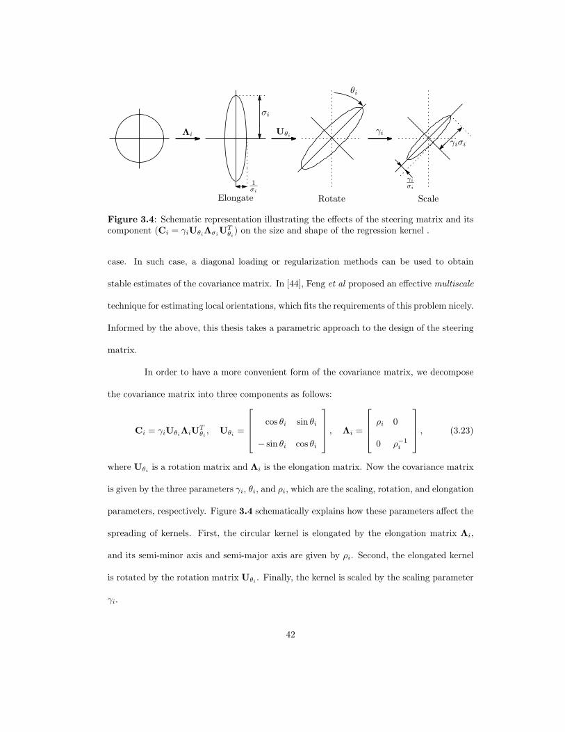
Λi Uθi
θi
σi
1σi
Elongate Rotate
γi
γiσi
γi
σi
Scale
Figure 3.4: Schematic representation illustrating the effects of the steering matrix and itscomponent (Ci = γiUθiΛσiU
Tθi
) on the size and shape of the regression kernel .
case. In such case, a diagonal loading or regularization methods can be used to obtain
stable estimates of the covariance matrix. In [44], Feng et al proposed an effective multiscale
technique for estimating local orientations, which fits the requirements of this problem nicely.
Informed by the above, this thesis takes a parametric approach to the design of the steering
matrix.
In order to have a more convenient form of the covariance matrix, we decompose
the covariance matrix into three components as follows:
Ci = γiUθiΛiUTθi
, Uθi =
⎡⎢⎢⎣ cos θi sin θi
− sin θi cos θi
⎤⎥⎥⎦ , Λi =
⎡⎢⎢⎣ ρi 0
0 ρ−1i
⎤⎥⎥⎦ , (3.23)
where Uθi is a rotation matrix and Λi is the elongation matrix. Now the covariance matrix
is given by the three parameters γi, θi, and ρi, which are the scaling, rotation, and elongation
parameters, respectively. Figure 3.4 schematically explains how these parameters affect the
spreading of kernels. First, the circular kernel is elongated by the elongation matrix Λi,
and its semi-minor axis and semi-major axis are given by ρi. Second, the elongated kernel
is rotated by the rotation matrix Uθi . Finally, the kernel is scaled by the scaling parameter
γi.
42

This thesis defines the scaling, elongation, and rotation parameters as follows.
Following the orientation estimation method in [44], the dominant orientation of the local
gradient field is the singular vector corresponding to the smallest (non-zero) singular value
of the local gradient matrix arranged in the following form
Gi =
⎡⎢⎢⎢⎢⎢⎢⎣...
...
zx1(xj) zx2(xj)
......
⎤⎥⎥⎥⎥⎥⎥⎦ = UiSiVTi , x ∈ wi, (3.24)
where UiSiVTi is the truncated singular value decomposition of Gi. Si is a diagonal 2 × 2
matrix representing the energy in the dominant directions. Then, the second column of the
orthogonal 2 × 2 matrix Vi, v2 = [ν1, ν2]T , gives the dominant orientation angle θi:
θi = arctan(
ν1
ν2
). (3.25)
That is, the singular vector corresponding to the smallest non-zero singular value of Gi
represents the dominant orientation of the local gradient field. The elongation parameter
ρi can be selected corresponding to the energy of the dominant gradient direction:
ρi =s1 + λ′
s2 + λ′ , λ′ ≥ 0, (3.26)
where λ′ is a regularization parameter for the kernel elongation, which dampens the effect
of the noise, and restricts the denominator away from becoming zero. The intuition behind
(3.26) is to keep the shape of the kernel circular in flat area (s1 ≈ s2 ≈ 0), and elongate it
near edge areas (s1 s2). Finally, the scaling parameter γi is defined by
γi =(
s1s2 + λ′′
M
) 12
, (3.27)
where λ′′ is again a regularization parameter, which dampens the effect of the noise and
keeps γi from becoming zero; and M is the number of samples in the local analysis window.
43

Figure 3.5: Footprint examples of steering kernels with covariance matrices Ci given bythe local orientation estimate (3.23) at a variety of image structures.
The intuition behind (3.27) is that, to reduce noise effects while producing sharp images,
large footprints are preferred in the flat (smooth) areas and smaller ones in the textured
areas. Note that the local gradients, as well as the eigenvalues (or singular values) of the
covariance matrix Ci, are smaller in the flat (low-frequency) areas than the textured (high-
frequency) areas. As the scaling parameter γi is given by the geometric mean of the singular
values of Ci in (3.27), γi makes the steering kernel area large in the flat areas, and small in
the textured areas. Figure 3.5 illustrates such behaviors of steering kernels at a variety of
image structures of Lena.
While it appears that the choice of three parameters in the above discussion is
44
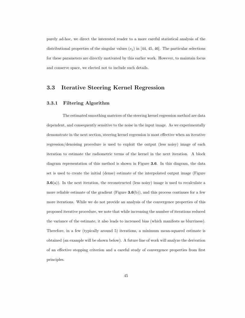
purely ad-hoc, we direct the interested reader to a more careful statistical analysis of the
distributional properties of the singular values (sj) in [44, 45, 46]. The particular selections
for these parameters are directly motivated by this earlier work. However, to maintain focus
and conserve space, we elected not to include such details.
3.3 Iterative Steering Kernel Regression
3.3.1 Filtering Algorithm
The estimated smoothing matrices of the steering kernel regression method are data
dependent, and consequently sensitive to the noise in the input image. As we experimentally
demonstrate in the next section, steering kernel regression is most effective when an iterative
regression/denoising procedure is used to exploit the output (less noisy) image of each
iteration to estimate the radiometric terms of the kernel in the next iteration. A block
diagram representation of this method is shown in Figure 3.6. In this diagram, the data
set is used to create the initial (dense) estimate of the interpolated output image (Figure
3.6(a)). In the next iteration, the reconstructed (less noisy) image is used to recalculate a
more reliable estimate of the gradient (Figure 3.6(b)), and this process continues for a few
more iterations. While we do not provide an analysis of the convergence properties of this
proposed iterative procedure, we note that while increasing the number of iterations reduced
the variance of the estimate, it also leads to increased bias (which manifests as blurriness).
Therefore, in a few (typically around 5) iterations, a minimum mean-squared estimate is
obtained (an example will be shown below). A future line of work will analyze the derivation
of an effective stopping criterion and a careful study of convergence properties from first
principles.
45

Gradient Est.Smoothting
Kernel Reg.yH(0)
i β(0)
1
Z(0)
(a) Initialization
SmoothingKernel Reg.
H(n+1)i β
(n+1)
1
Z(n+1)
β(n)
1
(b) Iteration
Noisy data
Z(n)
InitialMatrix Est.
Matrix Est.
Figure 3.6: Block diagram representation of the iterative adaptive regression.
It is worth pointing out that the iterative regression method has the luxury of
using directly estimated gradients. Note that the discrete gradients used in (3.24) are usually
approximated by convolving a bandpass filter with the image. However, comparison of (2.16)
and (2.19) shows that the vector β1 is the direct estimate of the image gradients. Indeed, the
direct estimation of the gradient vector is more reliable but at the same time computationally
more expensive. In Appendix B, computation of β1, directly in the regression context, is
presented.
3.3.2 Performance Analysis
In this section, we illustrate some properties and performance of iterative steering
kernel regression with a simple image denoising example. Adding white Gaussian noise with
standard deviation 25 to Figure 3.7(a) generates the noisy image shown in Figure 3.7(b).
The denoising results by the iterative steering kernel regression method with h = 2.75 are
illustrated in Figures 3.7(c)-(f). As seen in these results, the mean square error (MSE) is
minimized after 3 iterations. However, too many iterations result in the blurry image. As
we will illustrate shortly, this blur is caused by increasing bias in the estimate. On the other
46

hand, the variance is reduced with each iteration. It is known (q.v. [16]) that the mean
square error is expressed as
MSE [z(x, h)] = Bias2[z(x, h)] + Var [z(x, h)] , (3.28)
and the graph in Figure 3.8 illustrates the behavior of MSE, bias, and variance, which are
yielded by Monte Carlo simulations (100 denoising experiments per pixel by adding white
Gaussian noise with variance 25 and different noise seeds).
While in this case, choosing h = 2.75, with 3 iterations yielded the best estimate,
the necessary number of iterations is different for different h. Figure 3.10, Figure 3.11, and
Figure 3.12 illustrate the behavior of MSE, bias, and variance, respectively, and Table 3.1
shows the best estimates with for four different global smoothing parameters. Interestingly,
the best MSE’s are nearly the same even though the smoothing parameters are not. However
the ratio of bias and variance is different in each case. The larger the smoothing parameter
(h), the fewer iterations are necessary to reach the minimum MSE. With a larger h, however,
the estimated image has larger bias, which means the resulting image is more blurry. Figure
3.9 shows that two denoised results with a smaller h(= 2.25) and a larger h(= 3.0). As
Table 3.1 tells us, with the larger h, the estimated image (Figure 3.9(b)) is more blurry
than Figure 3.9(a), nonetheless their MSE are quite close. In general, a smaller h and more
iterations give us a visually superior result.
3.4 Summary
This chapter presented data-adapted (non-linear) kernel regression with two new
approaches: the bilateral kernel and the steering kernel, for image processing and reconstruc-
tion based on kernel regression. Moreover, a novel iterative filtering algorithm (Figure 3.6)
47

h 2.25 2.50 2.75 3.00it # 9 5 3 2MSE 101.35 98.87 98.33 98.93Bias2 46.70 49.22 51.29 54.82
Variance 54.65 49.65 47.04 44.11
Table 3.1: The best estimation in mean square error by iterative steering kernel regressionwith different global smoothing parameters.
and its performance are also presented. Using the data-adapted kernel regression method
with the iterative filtering algorithm, estimated images will have superior quality, which will
be demonstrated with real data sets in Chapter 5.
In the next chapter, we will discuss the application of ideas presented so far to
motion estimation. As reviewed in Section 1.2, to reconstruct a high quality image, we
need to have motions as accurately as possible. Surprisingly, the kernel regression method
has a power to improve the estimation performance of the current state of the art motion
estimation methods which use optical flow in a multi-resolution context.
48

(a) Original image (b) Noisy image, σ = 25
(c) Initial estimation, MSE=131.28 (d) 3 iterations, MSE=98.33
(e) 6 iterations, MSE=112.07 (f) 9 iterations, MSE=134.99
Figure 3.7: A denoising experiment by iterative steering kernel regression.
49
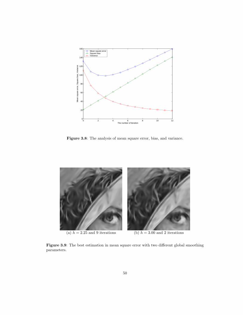
0 2 4 6 8 10 120
20
40
60
80
100
120
140
160
The number of iteration
Mea
n sq
uare
err
or, S
quar
e bi
as, V
aria
nce
Mean square errorSquare biasVariance
Figure 3.8: The analysis of mean square error, bias, and variance.
(a) h = 2.25 and 9 iterations (b) h = 3.00 and 2 iterations
Figure 3.9: The best estimation in mean square error with two different global smoothingparameters.
50

0 2 4 6 8 10 1280
100
120
140
160
180
200
The number of iteration
Mea
n sq
uare
err
or
h=2.25h=2.50h=2.75h=3.00
Figure 3.10: Mean square error with different global smoothing parameters.
0 2 4 6 8 10 120
20
40
60
80
100
120
140
160
180
200
The number of iteration
Squ
are
bias
h=2.25h=2.50h=2.75h=3.00
Figure 3.11: Bias with different global smoothing parameters.
51
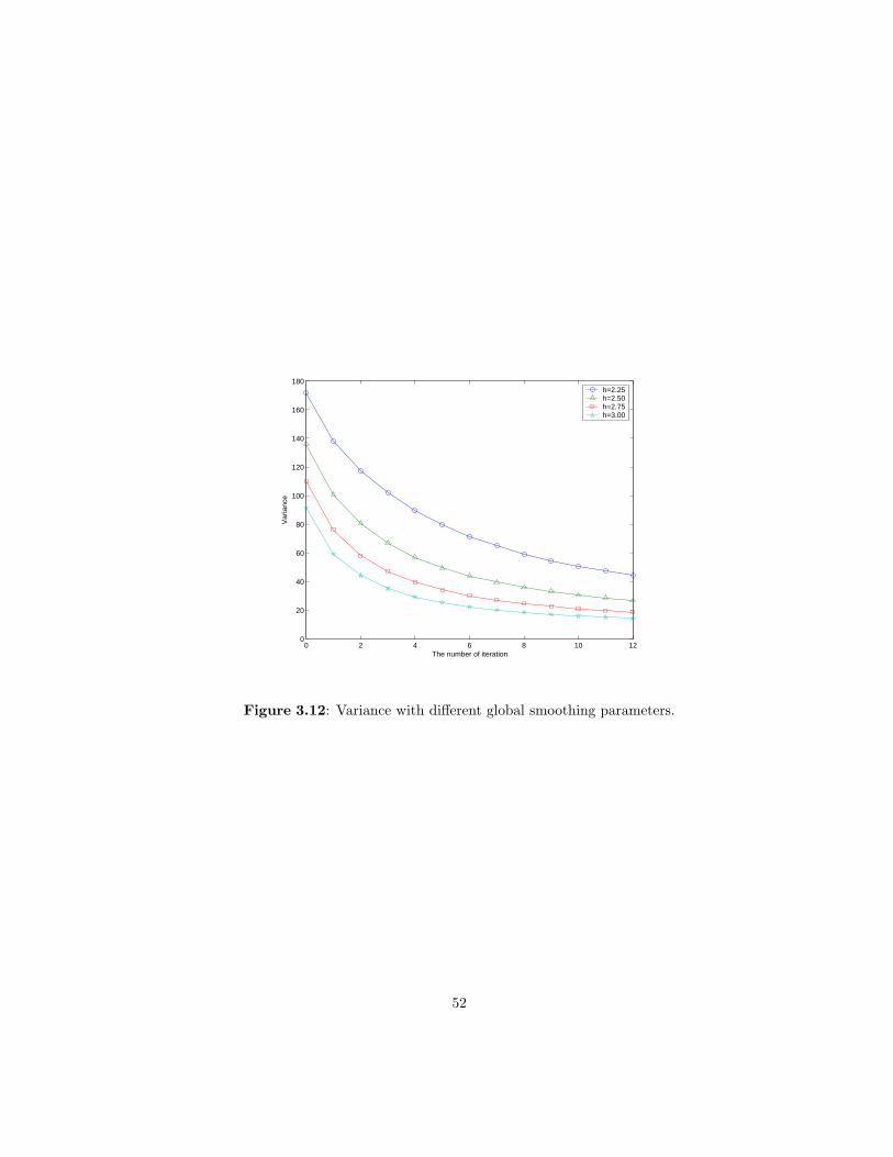
0 2 4 6 8 10 120
20
40
60
80
100
120
140
160
180
The number of iteration
Var
ianc
e
h=2.25h=2.50h=2.75h=3.00
Figure 3.12: Variance with different global smoothing parameters.
52

Chapter 4
Motion Estimation
4.1 Introduction
Motion estimation is one of the most important issues in image reconstruction, or
super-resolution. Once the motions are available, we know where measured data must be
located. After that we place all data onto a finer resolution grid, and interpolate them to
have a high quality image; a concept we reviewed in Section 1.2. In this chapter, we review
a widely-used motion estimation algorithm first (optical flow + multiscale) and then will
see how kernel regression makes the performance better.
Before going through the review of motion estimation, let’s remark on what factors
affect the performance. Motion estimation based on optical flow equations [8] is severely
influenced by measurement noise since the equations are built up on image gradients. And
when computing the gradients, we tend to amplify the noise. Moreover, computing correct
gradients is not so easy. Using sobel gradient operator [10], the estimated gradients have
errors [47], and such errors cause motion estimation errors. Hence, estimating gradients
53

itself is an important problem, and fortunately we can use higher order kernel regression
as a gradient estimator. The second order regression is a preferable choice to estimate the
first derivatives since the second derivative term β2 implicitly regularizes the first derivative
term β1. There is another problem that makes motion estimation difficult. Using multiscale
algorithm to cope with large motions, we propagate a motion estimated in coarse resolu-
tion fields to fine resolution fields. This propagation requires that we warp images by some
method, such as cubic spline interpolation. This image warping is, therefore, also affecting
the performance of motion estimation due to the distortion introduced by the image warp-
ing methods. To summarize, there are three factors which complicate motion estimation.
Namely: measurement noise, gradient errors, and image warping. Kernel regression is an
excellent tool to deal with these problems and will give us denoised and warped gradients
with a high quality.
We will deal with only translational motion [7] in this thesis. However the algorithm
is, of course, applicable to more complex parametric motion estimation. Translation is
the simplest motion model, in which we assume that all motions at every pixel are same,
and consequently there are two unknown motion parameters in the vertical and horizontal
directions.
4.2 Accurate Motion Estimation
4.2.1 Motion Estimator Based on Optical Flow Equations
In the first instance, we review briefly the motion estimation based on optical flow
equations. Suppose y(x, t) is the pixel value at x = [x1, x2]T and time t. A point in a frame
at x moves to x + d at the time t + dt, where d = [dx1 , dx2 ]T . Assuming constancy in the
54

pixel’s brightness, we can write the following equation:
y(x + d, t + dt) = y(x, t), (4.1)
where dx1 , dx2 and dt are assumed small. If these differential values are small enough to
neglect the higher order terms of a Taylor expansion, we have:
y(x + d, t + dt) ≈ y(x, t) +∂y
∂x1dx1 +
∂y
∂x2dx2 +
∂y
∂tdt. (4.2)
By comparing (4.1) with (4.2), we obtain
∂y
∂x1dx1 +
∂y
∂x2dx2 +
∂y
∂tdt = 0. (4.3)
Dividing both sides by dt, we arrive at
∂y
∂x1vx1 +
∂y
∂x2vx2 +
∂y
∂t= 0. (4.4)
This is the optical flow equation for a point x. Assuming constant vx1 , vx2 , We have as many
optical flow equations as the number of pixels of a frame, while the number of unknown
parameters is only two; namely vx1 and vx2 . Therefore, motion estimation in this case is
always an overdetermined problem. While this is encouraging, due to measurement noise
and gradient errors, motion estimation can still be unstable.
Suppose we have a pair of frames #n and #n + 1. The motion from the frame
#n to #n + 1 we call the forward motion. Analogously, from #n + 1 to #n, we have the
backward motion in the opposite direction. Figure 4.1 indicates the forward and backward
motion schematically. The magnitude of the (estimated) forward and backward motions
should the be same, but the directions are opposite. Using this property, we construct the
optical flow constraint. The optical flow equations of the forward motion between the nth
and (n + 1)th frames can be expressed in the vector form as
Y(n)x1
vx1 + Y(n)x2
vx2 + Y(n)t = 0, (4.5)
55

tx2
x1
t
t + dt
t − dt
forward
backward
frame #n
frame #n + 1
frame #n − 1
Figure 4.1: The forward and backward motion.
where the underline is the operator lexicographically ordering the elements of a matrix, and
Y(n)x1
=∂Yn
∂x1, Y(n)
x2=
∂Yn
∂x2, Y(n)
t =∂Yn
∂t≈ Yn − Yn+1. (4.6)
For the backward motion, we have
Y(n+1)x1
vx1 + Y(n+1)x2
vx2 − Y(n)t = 0. (4.7)
By combining (4.5) and (4.7)⎡⎢⎢⎣ Y(n)x1
Y(n+1)x1
⎤⎥⎥⎦ vx1 +
⎡⎢⎢⎣ Y(n)x2
Y(n+1)x2
⎤⎥⎥⎦ vx2 +
⎡⎢⎢⎣ Y(n)t
−Y(n)t
⎤⎥⎥⎦ = 0. (4.8)
Thus by incorporating this symmetry constraint, the number of optical flow equation is
doubled now. This idea can by applicable in any motion models based on optical flow
equations, and the result is more stable. For convenience let us rewrite (4.8) as
Jx1vx1 + Jx2
vx2 + Jt = 0, (4.9)
⇒ C(v) ≡ Jv + Jt = 0, (4.10)
56

where J =[Jx1
Jx2
]and v = [vx1 vx2 ]
T is the motion vector. We call C(v) the symmetric
optical flow constraint from now on.
Now we drive our translational motion estimator based on the optical flow con-
straint (4.10). Least squares estimator is a widely-used choice and the estimator is written
as
v = arg minv
∥∥∥Jv + Jt
∥∥∥2
2= arg min
v
(Jv + Jt
)T(Jv + Jt
), (4.11)
= −(JTJ)−1
JT Jt. (4.12)
However this estimator does not work well if the motion is large, we derived it under the
assumption that motions are small. To overcome this drawback of the estimator, multiscale
motion estimation are currently widely used (q.v. [48]). In the next section, we review it.
4.2.2 Multiscale Motion Estimation
For large motions, the approximation of (4.2) becomes inaccurate and inconsistent.
In order to overcome this difficulty, we construct pyramids as illustrated in Figure 4.2, each
scale of which is obtained by blurring with a low-pass filter (preferably Gaussian) and
downsampling with the factor of 2 for both vertical and horizontal directions. First, we
estimate the motion between the anchor and target frame in the top scale since the motion
is diminished in that scale, and hence the approximation of (4.2) works well. Now we have
a rough motion vector. After that we go down to one-lower scale and propagate the rough
motion to the scale. In other words, we warp (shift) the anchor or target image at that
scale, so that the motion between the two frames becomes small. Then we perform motion
estimation (4.12) again on that scale. We repeat this until arriving at the bottom scale. In
57

v2
v1
v0
anchor frame target frameYn Yn+1
Figure 4.2: Multiscale motion estimation
this way, the final motion vector is given by
v =L∑
l=0
2lvl, (4.13)
where L is the number of scales.
Using the multiscale motion estimation as mentioned above, we can deal with large
motions. However, in order to estimate motions more accurately in each scale, we perform
motion estimate iteratively several times in the same scale. The algorithm is simple; repeat-
ing motion estimation and image warping at the same scale. In that way, the motion to be
estimated between anchor and target frames are small, and consequently the approximation
(4.2) becomes more precise. Figure 4.3 illustrates the block diagram of the accurate motion
estimation in a scale. As the number of iterations increases, the estimated motion v between
anchor and warped target are smaller. We put µ (in Figure 4.3) as a damping factor to
make the estimation process stable, and it takes a value of 0 < µ ≤ 1.0. We do the iteration
58

Motionestimation
Warp
µv
v(n)l
v(n)l
v(n+1)l
Anchor
Target
propagate it toone lower scale
Figure 4.3: The block diagram of accurate motion estimation on a scale.
until the motion vector converges1, put it differently, until v becomes close to 0.
4.3 Image Warping
If the elements of the motions were integer number, it would be very easy for us to
warp images, since we could just shift the pixel to be neighboring pixels. However we need
a motion with sub-pixel accuracy, and this demands precise image warping. Well-known
image warping techniques are bilinear and cubic spline interpolation. As an attractive alter-
native, we present a new warping technique, based on kernel regression. Interestingly, kernel
regression can be an image warping tool, and it has great possibility, since the regression
estimates denoised, less inconsistent, warped derivatives directly. In the next section, the
performance analysis with different warping techniques are demonstrated.1It hopefully will converge. There is no guarantee. This issue must be investigated in the future work.
59

· · ·
Frame #1 Frame #2 Frame #20
Figure 4.4: A simulated sequence.
4.4 Simulations
This section examines the performance of motion estimation. Using the motion
estimation algorithm of Figure 4.3 with some different warping methods: (1)linear inter-
polation2, (2)cubic interpolation3, (3)classic kernel regression (N = 2 and h = 0.7 with
Gaussian kernel), we illustrate which method is better using noisy sequences. The noisy
sequence4 is generated by adding white Gaussian noise with a variety of standard devia-
tions to the simulated sequence shown in Figure 4.4. We generated the simulated sequence
by the following procedures: (1) take the convolution the original high resolution image
(1200 × 1200) with a 5 × 5 Gaussian kernel with variance 1.5, (2) randomly shift (integer
shift) the blurry image to the vertical and horizontal directions (translational motion), (3)
downsample the shifted image with factor 20 for both the vertical and horizontal directions
(4) do the procedure (1)-(3) 20 times. The experimental result (100 times Monte Carlo
simulations) is shown in Figure 4.5. The performance of the multiscale optical flow motion
estimations with linear and cubic warping are very close to each other. On the other hand,
the motion estimation with classic kernel regression yields us more accurate results.2MATLAB’s function “interp2” with the ’linear’ option.3MATLAB’s function “interp2” with the ’cubic’ option.4The corresponding signal to noise ratio is 9[dB] when the standard deviation is 20.
60

0 2 4 6 8 10 12 14 16 18 200.005
0.01
0.015
0.02
0.025
0.03
0.035
Standard deviation
Roo
t mea
n sq
uare
err
or
Linear interpolationCubic interpolationClassic kernel regression
Figure 4.5: The performance analysis of motion estimations with different warpingmethods.
4.5 Summary
In this chapter, we investigated accurate motion estimation, and showed that ker-
nel regression has great potential for use as image warping for motion estimation. The
simulations demonstrated the performance improvements.
61

Chapter 5
Demonstration and Conclusion
5.1 Introduction
In this chapter, we demonstrate how suitable the kernel regression technique is
for image processing and reconstruction. To show the ability of the proposed algorithm
in Chapter 3, we present three different applications: denoising, interpolation, and super-
resolution.
5.2 Image Denoising
In the first set of experiments, we compare the performance of several denoising
techniques. We set up a controlled simulated experiment by adding white Gaussian noise
with standard deviation (STD) of σ = 25 to the Lena image shown in Figure 5.1(a). The
resulting noisy image with PSNR1 of 20.17[dB], is shown in Figure 5.1(b). This noisy image
1Peak Signal to Noisy Ratio is defined as 20 log10
`255
RMSE
´.
62

is then denoised by the spline smoother2 of (2.13) with3 λ = 0.43, result of which is shown in
Figure 5.1(c) (zoomed in Figure 5.2(a)). The result of applying the bilateral filter (3.4) with
hs = 1.5 and hr = 7.4 is shown in Figure 5.1(d) (zoomed in Figure 5.2(b)). For the sake
of comparison, we have included the result of applying the recent wavelet based denoising
method4 of [49] in Figure 5.1(e) (zoomed in Figure 5.2(c)). Finally, Figure 5.1(f) (zoomed
in Figure 5.2(d)) shows the result of applying the iterative steering kernel regression of
Section 3.2.2 (N = 2, h = 2.4, and 7 iterations). The RMSE values of the reconstructed
images of Figure 5.1(b)-(f) are 25.0, 8.91, 8.65, 6.64, and 6.66, respectively.
We set up a second controlled simulated experiment by adding JPEG compression
artifacts to the uncompressed image of Figure 5.3(a). The JPEG image was constructed
by using MATLAB JPEG compression routine with a quality parameter equal to 10. This
compressed image with a RMSE value equal to 9.76 is illustrated in Figure 5.3(b). We
applied several denoising methods (similar to the ones used in the previous experiment) to
acquire higher quality estimates. The results of applying the spline smoother with λ = 0.11,
bilateral filter (3.4) with hs = 2.0 and hr = 4.1, wavelet [49], and the iterative steering kernel
regression (N = 2, h = 2.0 and 3 iterations) are given in Figure 5.3(c)-(f), respectively. The
RMSE values of the reconstructed images of Figure 5.3(c)-(f) are 9.05, 8.52, 8.80, and 8.48,
respectively.
In the third denoising experiment, we applied several denoising techniques on the
color image shown in Figure 5.4(a), which is corrupted by real film grain noise and scanning
process noise. To produce better color estimates, following [50], first we transferred this RGB
image to the YCrCb representation. Then we applied several denoising techniques (similar
2We used MATLAB’s spline smoother function “csaps”, for this and other spline smoother experiments.3The criteria for parameter selection in this example (and other examples discussed in this thesis) was
to choose parameters which produce visually most appealing results.4In this experiment, we used the code (with parameters suggested for this experiment) provided by the
author of [49] available at http://decsai.ugr.es/∼javier/denoise/index.html .
63

to the ones in the previous two experiments) on each channel (the luminance component
Y, and the chrominance components Cr and Cb), separately. The results of applying
Wavelet [49], and bilateral filter (3.4) (hs = 2.0 and hr = 3.5 for all the channels), and the
iterative steering kernel regression (N = 2, h = 2.0, and 3 iterations) are given in Figures
5.4(b)-(d), respectively. Figures 5.4(e)-(g) show the absolute values of the residuals in the
Y channel. It can be seen that the proposed steering kernel method produces the most
noise-like residuals.
5.3 Image Interpolation
In the forth experiment, we downsampled the Lena image of Figure 5.1(a) (zoomed
in Figure 5.6(a)) by a factor of 3 in each direction. The resulting aliased image is shown
in Figure 5.5(a). We compare the performance of different techniques, for upscaling this
(regularly sampled) image back to its original size (with the resolution enhancement factor
of 3 in each direction). Figure 5.5(b) (zoomed in Figure 5.6(b)) shows the result of applying
the spline smoother with λ = 0.0006. Figure 5.5(c) (zoomed in Figure 5.6(c)) is the result of
using the classic kernel regression (h = 1.75). Figure 5.5(d) (zoomed in Figure 5.6(d)) shows
the result of implementing the bilateral kernel regression of Section 3.2.1 (N = 0, hs = 1.75
and hr = 3.0). Figures 5.5(e) and (f) (zoomed in Figures 5.6(e) and (f), respectively) are
the results of the iterative steering kernel regression (N = 0, h = 1.0 and no iterations) and
(N = 2, h = 1.25 and no iterations) of Section 3.2.2. The RMSE values of the reconstructed
images of Figures 5.5(b)-(f) are 7.92, 7.96, 8.07, 8.03, and 7.42, respectively.
The fifth experiment is a controlled simulated regression of an irregularly sampled
image. We randomly deleted 85% of the pixels in the Lena image of Figure 5.1(a), creating
the sparse image of Figure 5.7(a). To fill the missing values, first we implemented the
64

Delaunay-spline smoother5 with λ = 0.087 to fill the missing values, the result of which is
shown in Figure 5.7(b), with some clear artifacts on the edges. Figure 5.7(c) shows the result
of using the classic kernel regression (2.36) (N = 2 and h = 2.25). The result of the bilateral
kernel regression (N = 0, hs = 2.25, and hr = 3.0) is shown in Figure 5.7(d). Figures 5.7(e)-
(f) show the results of implementing iterative steering kernel regression (N = 0, h = 0.8,
and no iterations), and (N = 2, h = 1.6, and 1 iteration), respectively. The RMSE values
for images in Figures 5.7(b)-(f) are 9.15, 9.69, 9.72, 8.91, and 8.21, respectively.
5.4 Super-Resolution
The sixth experiment is a multi-frame resolution enhancement (see Figure 2.6) of
a real compressed gray-scale video sequence captured with a commercial webcam (3COM,
Model no.3718). A total of 53 frames were captured with the camera, where the underlying
motion was assumed to follow the translational model, and motions are estimated by the
algorithm introduced in Chapter 4. The first frame of the sequence is shown in Figure
5.9(a) We used the spline smoother with λ = 0.01 to interpolate this image by the resolution
enhancement factor of 5 in each direction, as shown in Figure 5.9(b). To produce better
estimates, first we fused these frame on a high-resolution grid with 5 times more pixels in
each direction (shift-and-add method of Figure 1.2) and then interpolated the missing pixel
values. The result of interpolating the shift-and-add image by the Delaunay-spline smoother
with λ = 0.01, and the proposed steering kernel regression method of Section 3.2.2 with the
order of 2 and h = 1.0, are shown in Figure 5.9(c)-(d), respectively.
The last experiment is a multi-frame super-resolution of a real compressed color5To implement the Delaunay-spline smoother we used MATLAB’s “griddata” function with “cubic”
parameter to transform the irregularly sampled data set to a dense regularly sampled one (Delaunay trian-gulation). The quality of the resulting image was further enhanced by applying MATLAB’s spline smootherroutine “csaps”.
65

image sequence captured with a commercial video surveillance camera; courtesy of Adyoron
Intelligent Systems, Ltd., Tel Aviv, Israel. A total of 10 frames were used for this exper-
iment, where the underlying motion was assumed to follow the translational model. One
of these frames is shown in Figure 5.10(a). To produce better color estimates, following
[50], first we transferred the RGB frames to the YCrCb representation, and treated each
channel separately, as we did in the third experiment of Section 5.2. We used the method
described in Chapter 4 to estimate the motion vectors. Then, we fused each channel of
these frames on a high-resolution grid with 5 times more pixels as illustrated in Figure 1.2,
interpolated the missing values, and then deblurred the interpolated image using Bilateral
Total Variation regularization6 [6]. The result of interpolating the irregularly sampled image
by the Delaunay-spline smoother (implementation similar to the previous experiment with
λ = 0.5 for the luminance and λ = 1.0 for the chrominance channels) followed by deblurring
is shown in Figure 5.10(b). The results of applying the classic kernel regression (N = 2
and h = 2.0 for the luminance channel and h = 3.5 for the chrominance channels) followed
by deblurring and the iterative steering kernel regression (N = 2, h = 4.0 for the luminance
channel and h = 8.0 for the chrominance channels, and 1 iteration) followed by deblurring
are shown in Figures 5.10(c)-(d), respectively. Comparison of these diverse experiments
demonstrate that the proposed iterative steering kernel method not only performs best in a
quantitative sense but also results in sharper images with fewer artifacts.
5.5 Conclusion
In this thesis, we studied a non-parametric class of regression methods. We rein-6For this experiment the camera point spread function (PSF) was assumed to be a 5 × 5 Disk kernel
(obtained by the MATLAB command “fspecial(’disk’, 2)”). The deblurring regularization coefficientfor the luminance channel was chosen to be 0.2 and for the chrominance channels was chosen to be 0.5.
66

troduced kernel regression, as a general framework for studying several efficient denoising
and interpolation algorithms. We compared the similarities of the classic kernel regression
and another popular family of regressors, namely, spline smoother. We showed that the clas-
sic kernel regression in essence simplifies to a computationally efficient local linear filtering
process, the properties of which were studied under the topic of equivalent kernels.
To overcome the inherent limitations dictated by the linear filtering properties
of the classic kernel regression, we introduced the non-linear data-adapted class of kernel
regressors. We showed that the popular bilateral filtering technique is a special case of
data-adapted kernel regression. Later, we introduced and justified a novel adaptive kernel
regression method, called steering kernel regression, with superior performance as compared
to other regression method studied in this thesis. Experiments on simulated and real data
attested to our claim.
The superior performance of the data-adapted kernel regression can be explained by
noting that the spline smoother (2.13) in effect exploit the Tikhonov regularizers. However,
the data-adapted kernel regression in its simplest form (bilateral filter) exploits the Total
Variation (TV) regularization [51, 52]. The relation between the bilateral filtering and TV
regularization is established in [6]. The study in [6] also shows the superior performance of
the TV based regularization compared to the Tikhonov based regularization. More details
on the adaptive bilateral filters and their relation with the TV regularization can be found
in [6].
Finally, in Section 3.3, we proposed an iterative scheme to further improve the
performance of data-adapted kernel regression methods. Seeking an automatic method for
picking the optimal number of iterations or a stoping criterion for the iterations as well as
the optimal regression order is a part of our ongoing work.
67

(a) Original image (b) Noisy image, σ = 25
(c) Spline smoother (d) Bilateral filter
(e) Wavelet [49] (f) Iterative steering kernel
Figure 5.1: The performance of different denoising methods are compared in this experi-ment. The RMSE of the images (b)-(f) are 25, 8.91, 8.65, 6.64, and 6.66, respectively.
68

(a) Spline smoother (b) Bilateral filter
(c) Wavelet [49] (d) Iterative steering kernel
Figure 5.2: Figures 5.1(c)-(f) are enlarged to give (a),(b),(c), and (d), respectively.
69

(a) Original image (b) Compressed image
(c) Spline smoother (d) Bilateral Filtering
(e) Wavelet [49] (f) Iterative steering kernel
Figure 5.3: The performance of different denoising methods are compared in this exper-iment on a compressed image by JPEG format with the quality of 10. The RMSE of theimages (b)-(f) are 9.76, 9.05, 8.52, 8.80, and 8.48, respectively.
70

(a) Real noisy image (b) Wavelet [49]
(c) Bilateral filter (d) Iterative steering kernel555045403530252015105
(e) Wavelet [49] (f) Bilateral filter (g) Iterative steering kernel
Figure 5.4: The performance of different denoising methods are compared in this experi-ment on a color image with real noise. Gaussian kernel was used for all experiments.
71

(a) Downsampled Lena image (b) Spline smoother
(c) Classic kernel regression, N = 2 (d) Bilateral kernel regression, N = 0
(e) Steering kernel regression, N = 0 (f) Steering kernel regression, N = 2
Figure 5.5: Upscaling experiment. The image of Lena is downsampled by the factor of 3in (a). The factor of 3 up-sampled images of different methods are shown in (b)-(f). TheRMSE values for images (b)-(f) are 7.92, 7.96, 8.07, 7.93, and 7.43 respectively.
72

(a) Downsampled Lena image (b) Spline smoother
(c) Classic kernel regression, N = 2 (d) Bilateral kernel regression, N = 0
(e) Steering kernel regression, N = 0 (f) Steering kernel regression, N = 2
Figure 5.6: Figures 5.5(a)-(f) are enlarged to give (a)-(f), respectively.
73

(a) Irregularly downsampled image (b) Delaunay-spline smoother
(c) Classic kernel regression, N = 2 (d) Bilateral kernel regression, N = 0
(e) Steering kernel regression, N = 0 (f) Steering kernel regression, N = 2
Figure 5.7: Irregularly sampled data interpolation experiment, where 85% of the pixels inthe Lena image are omitted in (a). The interpolated images using different methods areshown in (b)-(f). RMSE values for (b)-(f) are 9.15, 9.69, 9.72, 8.91, and 8.21, respectively.
74

(a) Irregularly downsampled image (b) Delaunay-spline smoother
(c) Classic kernel regression, N = 2 (d) Bilateral kernel regression, N = 0
(e) Steering kernel regression, N = 0 (f) Steering kernel regression, N = 2
Figure 5.8: Figures 5.7(a)-(f) are enlarged to give (a)-(f), respectively.
75

(a) The first input frame (b) Single-frame Delaunay-spline smoother
(c) Multi-frame Delaunay-spline smoother (d) Multi-frame steering kernel regression
Figure 5.9: Image fusion (Super-Resolution) experiment of a real data set consisting of 10compressed grayscale images. One input image is shown in (a) which is up-scaled in (b)by the spline smoother interpolation. (c)-(d) show the multi-frame Shift-And-Add imagesafter interpolation by the Delaunay-spline smoother and the steering kernel methods. Theresolution enhancement factor in this experiment was 5 in each direction.
76

(a) The first input frame (b) Multi-frame Delaunay-spline smoother
(c) Multi-frame classic kernel regression (d) Multi-frame steering kernel regression
Figure 5.10: Image fusion (Super-Resolution) experiment of a real data set consisting of10 compressed color frames. One input image is shown in (a). (b)-(d) show the multi-frameShift-And-Add images after interpolating by the Delaunay-spline smoother, classical kernel,and steering kernel regression methods, respectively. The resolution enhancement factor inthis experiment was 5 in each direction.
77

Chapter 6
Super Resolution Toolbox
6.1 Introduction
This chapter explains the usage of the super resolution toolbox, which is the im-
plementation of the kernel regression technique described in this thesis. As we have seen
in Chapter 5, the technique can be applied for a wide class problems. Here, we explain
functions, which deal with denoising, interpolation, and fusion. Note that the function will
properly operate on MATLAB (version 6.5).
6.2 Installation
1. Extract the archive file “SuperResolutionToolBox.zip”, and copy the folder “Super-
ResolutionToolBox” to a folder (e.g. “C:/MATLAB6p5/work/”).
2. Start MATLAB, and set the path to the folder of “SuperResolutionToolBox” with
subfolders. As shown in Figure 6.1, first, pull down the file menu and click the “Set
Path...” illustrated in Figure 6.1(a). Second, following the circled number, set the
78

(a)(b)
Figure 6.1: Setting path.
path as illustrated in Figure 6.1(b).
6.3 The Kernel Regression Function
This section explains the function “KernelReg”. In the command line of MATLAB,
we run the function as follows:
[z, zx, zy] = KernelReg(frames, r, mvs, ref, Q, h, ktype, kfunc, ksize, it, wsize);
where z, zx, and zy are the output values: estimated images, estimated vertical gradient
images, and estimated horizontal gradient images, respectively. Table 6.1 explains the
parameters of the function. With this function, we can do denoising, interpolation, and
fusion. If the frames contain the color data in RGB, we must use the “KernelReg color”
function instead of calling the “KernelReg” function. Example usages are introduced in the
next section.
79

Params Descriptions Dimensionsframes Input frames (low resolution and noisy images) L×M×N
r Resolution enhancement factor scalarmvs Motion vectors (translational) 2×(N−1)
Please set mvs = [0, 0]T , when the number of frames is 1.ref The reference frame number scalarQ Regression order: 0 = constant, 1 = linear, or 2 = quadratic scalarh Global smoothing parameter
Classic kernel case, h scalarBilateral kernel case, h = [hs, hr]T 2 × 1Steering kernel case, h scalar
ktype Kernel type: ’ga’ = Gaussian, or ’exp’ = exponential (Laplacian) stringkfunc Kernel function: ’classic’, ’bilateral’, or ’steering’ stringksize Kernel window size (The window will be ksize× ksize.) scalar
it The number of iteration for iterative steering kernel regression scalarwsize The size of image analysis window for steering kernel regression scalar
Table 6.1: The parameter descriptions of “KernelReg” function.
6.4 Examples
There are several sample codes using the “KernelReg” function, which are located
in the folder named “examples”, under the folder of “SuperResolutionToolBox”. The codes
demonstrate the function with practical image processing examples. The details of the
example codes are written in the m-files, which are listed below.
• Gaussian noise removal (“Lena denoise.m”)
This example demonstrates Gaussian noise removal with the kernel regression tech-
niques discussed in this thesis: classic, bilateral and iterative steering kernel regression.
This produces the denoising results in Figure 5.1
• Compression artifact reduction (“Pepper deblock.m”)
This example demonstrates the compression artifact reduction. This program reads
an image and adds compression artifacts by saving the image in the JPEG format,
and reduces the artifacts using kernel regression. This produces the deblocking results
80
in Figure 5.3
• Film grain removal (“JFK denoise.m”)
This example demonstrates the denoising effect on a real noisy image (film grain noise).
Besides, the image is a color image so that this tells how to use the “KernelReg color”
function. This produces the denoising results shown in Figure 5.4
• Image upscale (“Lena upscale.m”)
This example demonstrates the image upscale on the Lena image in Figure 5.1(a).
The program first downsamples the Lena image with a downsampling factor, and then
upscales the given image with the same factor. This produces the upscaling results
shown in Figure 5.5.
• Image fusion (“tank8 fusion.m”)
This example demonstrates the simple image fusion and super-reslution on the tank
sequence in Figure 1.4. This produces the image fusion results shown in Fiture 2.7.
• Color super-resolution (“ady10 superresolution.m”)
This example demonstrates color super-resolution on a real noisy and severely com-
pressed vide sequence. This produces the color super-resolution results shown in Figure
5.10.
6.5 Troubleshooting
In the interpolation case, a reconstructed image with the function might have
some missing pixels. The problem can be solved by choosing appropriate parameter values.
Typically, the problem is caused by wrong choices of the resolution enhancement factor and
81
the global smoothing parameter. Either a smaller resolution enhancement factor or a larger
global smoothing parameter can overcome the trouble.
6.6 Summary
This chapter explained how to use the “KernelReg” function, and it is a conve-
nient tool for image processing and reconstruction. Only one function can do many things:
denoising, deblocking, upscaling, super-resolution, and so on.
82

Chapter 7
Future Work
7.1 Robust Kernel Regression
The classic kernel regression framework can be regarded as a weighted least square
estimator (q.v. Chapter 2). However, in the case that there are some outliers in a measured
data set, the estimator will strongly stick to those outliers due to the square error norm. In
order to overcome this problem, it is possible for us to modify the framework with the idea
of robust estimation. A more general, the robust framework for kernel regression may be
expressed as
minβnN
n=0
P∑i=1
Ω
(yi − β0 −βT
1 (xi −x)−βT2 vech
(xi −x)(xi −x)T
)K(xi −x, yi − y), (7.1)
where Ω(·) is the error norm function. The common selections of the function are illustrated
in Table 7.1. As an example of the usefulness of this more general framework, salt & pepper
noise reduction is illustrated in Figure 7.1. In this example, we added 20% salt and pepper
noise (outliers) to the original image of Figure 7.1(a), resulting in the noisy image of Figure
7.1(b). The denoised image using a 3 × 3 median filter, wavelet method of [49], l2 classic
83

(a) Original (b) Noisy (c) Median (d) Wavelet [49]
(e) l2 Classic (f) l2 Steering (g) l1 Classic (h) l1 Steering
Figure 7.1: An example of the salt & pepper noise reduction. Corresponding RMSE for(b)-(h) are 63.84, 11.05, 22.47, 21.81, 21.06, 7.65, and 7.14.
kernel regression (N = 2 and h = 2.46), l2 iterative steering kernel regression (N = 2,
h = 2.25 and 20 iterations), l1 classic kernel regression (N = 2 and h = 0.65), and l1
iterative steering kernel regression (N = 2, h = 2.25, and no iterations) are shown in
Figures 7.1(b)-(h), respectively. The performance difference is quite clear. By using the
l1 norm instead of the l2 norm, the kernel regression now successfully reduced the salt &
pepper noise. Besides, with the steering kernel, we have an even better estimated image.
84

Absolute (l1 Norm)Ω(x) = |x| Ω′(x) = sign(x)
−10 −8 −6 −4 −2 0 2 4 6 8 100
1
2
3
4
5
6
7
8
9
10
−10 −8 −6 −4 −2 0 2 4 6 8 10
−1
−0.8
−0.6
−0.4
−0.2
0
0.2
0.4
0.6
0.8
1
Quadratic (l2 Norm)Ω(x) = x2 Ω′(x) = 2x
−10 −8 −6 −4 −2 0 2 4 6 8 100
10
20
30
40
50
60
70
80
90
100
−10 −8 −6 −4 −2 0 2 4 6 8 10−20
−15
−10
−5
0
5
10
15
20
Truncated Quadratic
Ω(x, α, λ) =
λx2 |x| <√
αλ
α elseΩ′(x, α, λ) =
2λx |x| <
√αλ
0 else
−10 −8 −6 −4 −2 0 2 4 6 8 100
0.5
1
1.5
2
2.5
3
3.5
4
4.5
5
5.5
−10 −8 −6 −4 −2 0 2 4 6 8 10−1.5
−1
−0.5
0
0.5
1
1.5
Geman & McClureΩ(x, α) = x2
x2+α Ω′(x, α) = 2xα(x2+α)2
−10 −8 −6 −4 −2 0 2 4 6 8 100
0.2
0.4
0.6
0.8
1
−10 −8 −6 −4 −2 0 2 4 6 8 10−0.8
−0.6
−0.4
−0.2
0
0.2
0.4
0.6
0.8
Lorentzian
Ω(x, α) = log
1 + 12
(xα
)2 Ω′(x, α) = 2xx2+2α2
−10 −8 −6 −4 −2 0 2 4 6 8 100
0.5
1
1.5
2
2.5
3
3.5
4
−10 −8 −6 −4 −2 0 2 4 6 8 10−0.8
−0.6
−0.4
−0.2
0
0.2
0.4
0.6
0.8
Table 7.1: Error norm functions and their derivatives [1].
85

7.2 Segment Motion Estimation
7.2.1 Motivation
Motion estimation enables us to fuse images so that we can reconstruct a high
resolution image by using the kernel regression technique. However the larger the images
to fuse, the more difficult to estimate motions with a simple motion model. In this thesis,
we dealt with the simplest motion model, translational motion. It is obviously impossible
for this model to be assumed always valid. Even using the parametric (e.g. affine motion
model), camera lens distortion on the images depart from this simple model. Moreover, it
is definitely necessary for us to consider the motion flow occlusions. In this section, an idea
of the motion estimation for large images which may have occlusions will be discussed.
7.2.2 Image Segmentation
Since the motion estimation on large images is difficult, the intuitive way to over-
come this difficulty is to segment the images into small pieces, and then estimate motions
for each piece. There are several types of segmentation methods we must consider. The list
below is a sampling of these methods.
1. Fixed block base
This is the simplest segmentation method. With this method, we blindly segment
two images (reference and target images) into a collection of fixed-size blocks in the
same way, and estimate motions between every pair of corresponding blocks of the
reference image and the target image. Theoretically, the smaller the block size, the
more accurate the overall motion will be estimated; however, the local estimation
becomes more difficult and unstable.
86

2. Object or texture base
Motion flow occlusions often happen around the border areas of objects or textures.
Hence it is a good way for us to segment the images based on objects or textures, and
estimate the corresponding segments between the reference and the target image.
3. Motion base
The motion flow occlusions do not happen at all the objects’ borders. As we know
already, the larger the segment, the more stable the motion estimate will be. The
motion based segmentation method detects the occlusions and segment the image
accordingly. Although this is the most difficult method, once we implement and have
the motions, the reconstructed images will give superior results.
7.2.3 Motion Models
Motion models are also significantly important for successful motion estimation.
Since the translational model is often not flexible enough to fit unknown motions, with this
model, the only thing we can do to have a better parametric fit is to reduce the size of
the segment. However, again, the estimation becomes unstable due to the small number of
optical flow equations. Another way to proceed is to use more general parametric motion
models: affine, projective linear, and so on. Most likely, with a proper image segmentation
algorithm, the affine motion model is the most appropriate one. In the next section, one
simple demonstration is shown.
87

7.3 Example
In this section, we present a simple example of the image reconstruction from large
size frames. Figure 7.2 shows the three frames from a video sequence. The size of all the
frames is 350 × 600. Using the classic kernel regression (order N = 2, global smoothing
parameter h = 1.0, and resolution enhancement factor r = 2), we try to reconstruct a high
quality image from them. First, we reconstruct an image under the assumption that all the
pixels have the same linear motion (i.e. translational motion model). The result is given in
Figure 7.3. Since the global motion model is inaccurate, the upper and bottom part of the
reconstruction look blurry. Alternatively, we segment all the frames into fixed-size blocks
(50 × 50) and estimate motions for these blocks. The result is illustrated in Figure 7.4.
While this result too is not perfect, the quality is much better (sharper) than Figure 7.3.
7.4 Summary
This chapter showed another possibility of the kernel regression technique. In the
future, it is obvious that video to video super-resolution and dynamic super-resolution will
be focused.
88

(a) The first frame
(b) The second frame
(c) The thrid frame
Figure 7.2: Three large frames from a video sequence. The size of each frame is 350× 600.
89

Figure 7.3: The reconstructed image using the translational motion model.
90

Figure 7.4: The reconstructed image using the translational motion model with the blocksegmentation.
91

Appendix A
Image Deblurring
Image deblurring is the last phase of super-resolution, and it is necessary to recover
some high frequency components of fused images in most cases, since the images are usually
blurred by atmosphere and camera. Moreover, unfortunately, kernel regression1 also gives
some blurring effects to the images, particularly when we choose a wrong parameter (e.g.
unnecessarily large smoothness). Therefore image deblurring is necessary, and, in this sec-
tion, a simple deblurring method in the spatial domain is introduced. We leave the method
to remove spatial invariant blurring effects by adapted kernel regression as a future work.
Suppose we have a blurred image Z, which is given by a blurred version of a real
scene X, is expressed as
Z = BX + ε, (A.1)
where the matrix (image) with an underline is the column-stack vector of the matrix, B
is the blur operator, and ε is noise. Note that the estimated blurred image by kernel
regression has already removed much of the noise. Regularized least-squares estimator is a1Data-adapted kernel regression will give spatially variant blurring effects to estimated images
92

Tikhonov Total variation Bilateral total variation [6]
Υ(X) ‖ΓX‖22 ‖ΓX‖1
qXl=−q
qXm=−q
α|l|+|m|‚‚‚X − Sl
x1Smx2X
‚‚‚1
Υ′(X) 2ΓT ΓX ΓT sign(ΓX)
qXl=−q
qXm=−q
α|l|+|m|“I − S−l
x1S−mx2
”sign
“X − Sl
x1Smx2X
”
Table A.1: Regularization functions and their first derivatives.
typical choice for the real scene X, which takes the form
XRLS = arg minX
[∥∥∥BX − Z∥∥∥2
2+ λΥ (X)
]= arg min
XC (X) , λ ≥ 0, (A.2)
where Υ (X) is a regularization function. We minimize the cost function C (X) to find X
by the steepest descent method,
X(n+1)
= X(n) − µ
[BT
(BX
(n) − Z)
+ λΥ′(X
(n))]
. (A.3)
The choices of Υ (X) and their derivatives are listed up in Table A.1, in which Γ is a highpass
filter, (e.g. Laplacian), and S is the shift operator, and α is a parameter controlling the
decay of weights.
93

Appendix B
Local Gradient Estimation
As we mentioned several times, the higher order (N > 0) kernel regression used
for gradient estimation, which is very useful for image processing and reconstruction. As
we know already, gradient estimates can be used for orientation estimation and motion
estimation. In this section, local gradient estimators with the order of N = 1 and 2 are
derived. In the optimization problem (2.24), the term we wish to estimate is β1. Hence,
the gradient estimator is
∇z(x) = β1 =
⎡⎢⎢⎣ eT2
eT3
⎤⎥⎥⎦(XTxWxXx
)−1XT
xWxY, (B.1)
where e2 and e3 are column vectors (the same size of b in (2.25)) whose second and third
elements are 1 respectively, and the rest are zero. Following the notation of (2.29), the local
linear (N = 1) and local quadratic (N = 2) gradient estimators are given by
∇z(x) =P∑
i=1
[s22 − s21s
−111 s12
]−1 [−s21s−111 + (xi − x)
]KH(xi − x)yi (B.2)
∇z(x) =P∑
i=1
S−1[−S21S
−111 + (xi − x) − S23S
−133 vech
(xi − x)(xi − x)T
]KH(xi − x)yi,
(B.3)
94

respectively, where
S11 = s11 − s13s−133 s31, S21 = s21 − s23s−1
33 s31
S23 = s23 − s21s−111 s13, S33 = s33 − s31s
−111 s13, (B.4)
S = s22 − S21S−111 s12 − S23S
−133 s32. (B.5)
Of course it is absolutely possible for us to use adapted kernels (bilateral and steering kernels)
for the gradient estimators as well. Amazingly, this estimator also has great denoising
effect and can interpolate gradient images, consequently image warping is also possible
with it, therefore it is a suitable tool for motion estimation, too. For the super-resolution
experiments in Chapter 5, these estimators are used for motion estimation.
95

Bibliography
[1] M. J. Black and P. Anandan, “The robust estimation of multiple motions: Parametric
and piecewise-smooth flow fileds,” Computer Vision and Image Understanding, vol. 63,
no. 1, pp. 75–104, January 1996.
[2] H. Takeda, S. Farsiu, and P. Milanfar, “Image denoising by adaptive kernel regression,”
Proceedings of the 39th Asilomar Conference on Signals, Systems, and Computers,
Pacific Grove, CA, pp. 1660–1665, November 2005.
[3] ——, “Kernel regression for image processing and reconstruction,” submitted to IEEE
Transactions on Image Processing.
[4] ——, “Robust kernel regression for restoration and reconstruction of images from sparse
noisy data,” Invited paper, 2006 International Conference on Image Processing, At-
lanta, GA.
[5] T. F. Chan, “Nontexture inpainting by curvature-driven diffusions,” Journal of Visual
Communication and Image Representation, vol. 12, no. 10, pp. 436–449, May 2001.
[6] S. Farsiu, D. Robinson, M. Elad, and P. Milanfar, “Fast and robust multi-frame super-
resolution,” IEEE Transactions on Image Processing, vol. 13, no. 10, pp. 1327–1344,
October 2004.
96

[7] C. Stiller and J. Konrad, “Estimating motion in image sequences - a tutorial on mod-
eling and computation of 2d motion,” IEEE Signal Processing Magazine, vol. 16, no. 4,
pp. 70–91, July 1999.
[8] J. R. Bergen, P. Anandan, K. J. Hanna, and R. Hingorani, “Hierarchical model-based
motion estimation,” Proceedings of the European Conf. on Computer Vision, pp. 237–
252, May 1992.
[9] S. Farsiu, M. D. Robinson, M. Elad, and P. Milanfar, “Robust shift-and-add approach
to super-resolution,” Proceeding of the SPIE Annual Meeting, San Diego, CA, vol. 5203,
August 2003.
[10] R. C. Gonzalez and R. E. Woods, Digital Image Processing. Upper Saddle River, N.J.:
Prentice Hall, 2002.
[11] M. Unser, “Splines: A perfect fit for signal and image processing,” IEEE Signal Pro-
cessing Magazine, vol. 16, no. 6, pp. 22–38, November 1999.
[12] C. de Boor, A Practical Guide to Splines. New York: Springer-Verlag, 1978.
[13] E. A. Nadaraya, “On estimating regression,” Theory of Probability and its Applications,
vol. 9, pp. 141–142, September 1964.
[14] M. Elad and Y. Hel-Or, “A fast super-resolution reconstruction algorithm for pure
translational motion and common space-invariant blur,” IEEE Transactions on Image
Processing, vol. 10, no. 8, pp. 1187–1193, August 2001.
[15] A. Zomet, A. Rav-Acha, and S. Peleg, “Robust super-resolution,” Proceedings of the
International Conference on Computer Vision and Pattern Recognition (CVPR), 2001,
Hawaii.
97

[16] S. M. Kay, Fundamentals of Statistical Signal Processing - Estimation Theory -, ser.
Signal Processing Series. Englewood Cliffs, N.J.: PTR Prentice-Hall, 1993.
[17] M. P. Wand and M. C. Jones, Kernel Smoothing, ser. Monographs on Statistics and
Applied Probability. London; New York: Chapman and Hall, 1995.
[18] S. V. Huffel and J. Vandewalle, The Total Least Squares Problem: Computational As-
pects and Analysis, ser. Frontiers in applied mathematics. Philadelphia: Society for
Industrial and Applied Mathematics, 1991, vol. 9.
[19] P. Yee and S. Haykin, “Pattern classification as an ill-posed, inverse problem: a reglar-
ization approach,” Proceeding of the IEEE International Conference on Acoustics,
Speech, and Signal Processing, ICASSP, vol. 1, pp. 597–600, April 1993.
[20] V. N. Vapnik, Statistical Learning Theory, ser. Adaptive and learning systems for signal
processing, communications, and control. New York: Wiley, 1998.
[21] H. Knutsson and C.-F. Westin, “Normalized and differential convolution: Methods
for interpolation and filtering of incomplete and uncertain data,” Proceedings of IEEE
Computer Society Conference on Computer Vision and Pattern Recognition, pp. 515–
523, June 16-19 1993.
[22] T. Q. Pham, L. J. van Vliet, and K. Schutte, “Robust fusion of irregularly sampled
data using adaptive normalized convolution,” EURASIP Journal on Applied Signal
Processing, 2005.
[23] C. Tomasi and R. Manduchi, “Bilateral filtering for gray and color images,” Proceeding
of the 1998 IEEE International Conference of Compute Vision, Bombay, India, pp.
836–846, January 1998.
98

[24] M. Elad, “On the origin of the bilateral filter and ways to improve it,” IEEE Transac-
tions on Image Processing, vol. 11, no. 10, pp. 1141–1150, October 2002.
[25] D. Comaniciu and P. Meer, “Mean shift: A robust approach toward feature space
analysis,” IEEE Transactions on Pattern Analysis and Machine Intelligence, vol. 24,
no. 5, pp. 603–619, May 2002.
[26] X. Li and M. T. Orchard, “New edge-directed interpolation,” IEEE Transactions on
Image Processing, vol. 10, no. 10, pp. 1521–1527, October 2001.
[27] N. K. Bose and N. Ahuja, “Superresolution and noise filtering using moving least
squares,” submitted to IEEE Transactions on Image Processing, 2005.
[28] B. W. Silverman, Density Estimation for Statistics and Data Analysis, ser. Monographs
on Statistics and Applied Probability. London; New York: Chapman and Hall, 1986.
[29] W. Hardle, Applied Nonparametric Regression. Cambridge [England] ; New York:
Cambride University Press, 1990.
[30] W. Hardle, M. Muller, S. Sperlich, and A. Werwatz, Nonparametric and Semiparametric
Models, ser. Springer Series in Statistics. Berlin ; New York: Springer, 2004.
[31] W. Hardle, Smooting Technique with Implementation in S, ser. Springer Series in Statis-
tics. New York: Springer-Verlag, 1991.
[32] D. Ruppert and M. P. Wand, “Multivariate locally weighted least squares regression,”
The Annals of Statistics, vol. 22, no. 3, pp. 1346–1370, September 1994.
[33] M. G. Schimek, Smooting and Regression -Approaches, Computation, and Application-,
ser. Wiley Series in Probability and Statistics. New York: Wiley-Interscience, 2000.
99

[34] J. E. Gentle, W. Hardle, and Y. Mori, Handbook of Computational Statistics: Concepts
and Methods. Berlin ; New York: Springer, 2004, pp. 539–564 (Smoothing: Local
Regression Techniques).
[35] R. L. Eubank, Nonparametric Regression and Spline Smoothing, ser. Statistics, text-
books and monographs. New York: Marcel Dekker, 1999, vol. 157.
[36] L. Piegl and W. Tiller, The NURBS Book. New York: Springer, 1995.
[37] M. Arigovindan, M. Suhling, P. Hunziker, and M. Unser, “Variational image recon-
struction from arbitrarily spaced samples: A fast multiresolution spline solution,” IEEE
Transactions on Image Processing, vol. 14, no. 4, pp. 450–460, April 2005.
[38] B. W. Silverman, “Spline smoothing: The equivalent variable kernel method,” The
Annals of Statistics, vol. 12, no. 3, pp. 898–916, September 1984.
[39] J. A. Nelder and R. Mead, “A simplex method for function minimization,” Computer
Journal, vol. 7, no. 4, pp. 308–313, 1965.
[40] I. S. Abramson, “On bandwidth variation in kernel estimates - a square root law,” The
Annals of Statistics, vol. 10, no. 4, pp. 1217–1223, December 1982.
[41] A. Buades, B. Coll, and J. M. Morel, “On image denoising methods,” Technical Note,
CMLA (Centre de Mathematiques et de Leurs Applications), no. 5, 2004.
[42] K. Fukunaga, Introduction to Statistical Pattern Recognition, 2nd ed., ser. Computer
Science and Scientific Computing. Boston: Academic Press, 1990.
[43] R. O. Duda, P. E. Hart, and D. G. Stork, Pattern Classification, 2nd ed. New York:
Wiley-Interscience, 2001.
100

[44] X. Feng and P. Milanfar, “Multiscale principal components analysis for image local ori-
entation estimation,” Proceedings of the 36th Asilomar Conference on Signals, Systems
and Computers, Pacific Grove, CA, November 2002.
[45] K. V. Mardia, J. T. Kent, and J. M. Bibby, Multivariate Analysis. London ; New
York: Academic Press, 1979.
[46] A. Edelman, “Eigenvalues and condition numbers of random matrices,” SIAM Journal
on Matrix Analysis and Aplications, vol. 9, pp. 543–560, 1988.
[47] S. Ando, “Consistent gradient operators,” IEEE Transactions on Pattern Analysis and
Machine Intelligence, vol. 22, no. 3, pp. 252–265, March 2000.
[48] Y. Wang, J. Ostermann, and Y. Zhang, Video Processing and Communications. Upper
Saddle River, NJ: Prentice Hall, 2002.
[49] J. Portilla, V. Strela, M. Wainwright, and E. P. Simoncelli, “Image denoising using scale
mixtures of Gaussians in the wavelet domain,” IEEE Transactions on Image Processing,
vol. 12, no. 11, pp. 1338–1351, November 2003.
[50] S. Farsiu, M. Elad, and P. Milanfar, “Multiframe demosaicing and super-resolution of
color images,” IEEE Transactions on Image Processing, vol. 15, no. 1, pp. 141–159,
January 2006.
[51] L. Rudin, S. Osher, and E. Fatemi, “Nonlinear total variation based noise removal
algorithms,” Physica D, vol. 60, pp. 259–268, November 1992.
[52] T. F. Chan, S. Osher, and J. Shen, “The digital TV filter and nonlinear denoising,”
IEEE Transactions on Image Processing, vol. 10, no. 2, pp. 231–241, February 2001.
101