Embed Size (px)
Citation preview
Journal of Machine Learning Research () Submitted ; Published
Kernel-Based Reinforcement Learning UsingBellman Residual Elimination
Brett Bethke [email protected] of Aeronautics and AstronauticsMassachusetts Institute of TechnologyCambridge, MA 02139, USA
Jonathan P. How [email protected] of Aeronautics and Astronautics, MIT
Asuman Ozdaglar [email protected]
Department of Electrical Engineering and Computer Science, MIT
Editor:
Abstract
This paper presents a class of new approximate policy iteration algorithms for solvinginfinite-horizon, discounted Markov decision processes (MDPs) for which a model of thesystem is available. The algorithms are similar in spirit to Bellman residual minimizationmethods. However, by exploiting kernel-based regression techniques with nondegeneratekernel functions as the underlying cost-to-go function approximation architecture, the newalgorithms are able to explicitly construct cost-to-go solutions for which the Bellman resid-uals are identically zero at a set of chosen sample states. For this reason, we have namedour approach Bellman residual elimination (BRE). Since the Bellman residuals are zero atthe sample states, our BRE algorithms can be proven to reduce to exact policy iterationin the limit of sampling the entire state space. Furthermore, by exploiting knowledge ofthe model, the BRE algorithms eliminate the need to perform trajectory simulations andtherefore do not suffer from simulation noise effects. The theoretical basis of our approachis a pair of reproducing kernel Hilbert spaces corresponding to the cost and Bellman resid-ual function spaces, respectively. By construcing an invertible linear mapping betweenthese spaces, we transform the problem of performing BRE into a simple regression prob-lem in the Bellman residual space. Once the solution in the Bellman residual space isknown, the corresponding cost function is found using the linear mapping. This theoreticalframework allows any kernel-based regression technique to be used to perform BRE. Themain algorithmic results of this paper are two BRE algorithms, BRE(SV) and BRE(GP),which are based on support vector regression and Gaussian process regression, respectively.BRE(SV) is presented first as an illustration of the basic idea behind our approach, andthis approach is then extended to develop the more sophisticated BRE(GP). BRE(GP)is a particularly useful algorithm, since it can exploit techniques from Gaussian processregression to automatically learn the kernel parameters (via maximization of the marginallikelihood) and provide error bounds on the solution (via the posterior covariance). Exper-imental results demonstrate that both BRE(SV) and BRE(GP) produce good policies andcost approximations for a classic reinforcement learning problem.
Keywords: Kernel methods, Reinforcement learning, Approximate dynamic program-ming, Bellman residual elimination, Support vector regression, Gaussian process regression
c© Brett Bethke, Jonathan P. How, and Asuman Ozdaglar.
Bethke, How, and Ozdaglar
1. Introduction
Markov Decision Processes (MDPs) are a powerful framework for addressing problems in-volving sequential decision making under uncertainty (Bertsekas, 2007; Puterman, 1994).Such problems arise frequently in a number of fields, including engineering, finance, andoperations research. It is well-known that MDPs suffer from the curse of dimensionality,which implies that the size of the state space, and therefore the amount of time necessaryto compute the optimal policy, increases exponentially rapidly with the size of the problem.The curse of dimensionality renders most MDPs of practical interest very difficult to solveexactly using standard methods such as value iteration or policy iteration. To overcome thischallenge, a wide variety of methods for generating approximate solutions to large MDPshave been developed, giving rise to the field of reinforcement learning (sometimes also re-ferred to as approximate dynamic programming or neuro-dynamic programming) (Bertsekasand Tsitsiklis, 1996; Sutton and Barto, 1998).
Approximate policy iteration is a central idea in many reinforcement learning methods.In this approach, an approximation to the cost-to-go vector of a fixed policy is computed;this step is known as policy evaluation. Once this approximate cost is known, a policyimprovement step computes a new, potentially improved policy, and the process is repeated.In many problems, the policy improvement step involves a straightforward minimizationover a finite set of possible actions, and therefore can be performed exactly. However, thepolicy evaluation step is generally more difficult, since it involves solving the fixed-policyBellman equation:
TµJµ = Jµ. (1)
Here, Jµ represents the cost-to-go vector of the policy µ, and Tµ is the fixed-policy dynamicprogramming operator (these objects will be fully explained in the next section). Eq. (1) is alinear system of dimension |S|, where |S| denotes the size of the state space S. Because |S| istypically very large, solving Eq. (1) exactly is impractical, and an alternative approach mustbe taken to generate an approximate solution. Much of the research done in reinforcementlearning focuses on how to generate these approximate solutions, which will be denoted inthis paper by Jµ.
The accuracy of an approximate solution Jµ generated by a reinforcement learningalgorithm is important to the ultimate performance achieved by the algorithm. A naturalcriterion for evaluating solution accuracy in this context is the Bellman error BE:
BE ≡ ||Jµ − TµJµ|| =
(∑i∈S|Jµ(i)− TµJµ(i)|2
)1/2
. (2)
The individual termsJµ(i)− TµJµ(i)
which appear in the sum are referred to as the Bellman residuals. Designing a reinforcementlearning algorithm that attempts to minimize the Bellman error over a set of candidate costsolutions is a sensible approach, since achieving an error of zero immediately implies thatthe exact solution has been found. However, it is difficult to carry out this minimizationdirectly, since evaluation of Eq. (2) requires that the Bellman residuals for every statein the state space be computed. To overcome this difficulty, a common approach is to
2
Kernel-Based RL Using Bellman Error Elimination
generate a smaller set of representative sample states S (using simulations of the system,prior knowledge about the important states in the system, or other means) and work withan approximation to the Bellman error BE obtained by summing Bellman residuals overonly the sample states: (Bertsekas and Tsitsiklis, 1996, Ch. 6):
BE ≡
∑i∈ eS|Jµ(i)− TµJµ(i)|2
1/2
. (3)
It is then practical to minimize BE over the set of candidate functions. This approachhas been investigated by several authors, including (Schweitzer and Seidman, 1985; Baird,1995; Munos and Szepesvari, 2008; Antos et al., 2008), resulting in a class of reinforcementlearning algorithms known as Bellman residual methods.
The set of candidate functions is usually referred to as a function approximation archi-tecture, and the choice of architecture is an important issue in the design of any reinforce-ment learning algorithm. Numerous approximation architectures, such as neural networks(Hornik et al., 1989; Bishop, 1995; Haykin, 1994; Tesauro, 1995, 1992), linear architectures(Lagoudakis and Parr, 2003; Bertsekas and Tsitsiklis, 1996; Bertsekas, 2007; Si and Wunsch,2004; Bertsekas and Ioffe, 1996; de Farias and Van Roy, 2003; Valenti, 2007), splines (Trickand Zin, 1997), and wavelets (Maggioni and Mahadevan, 2006; Mahadevan and Maggioni,2005) have been investigated for use in reinforcement learning. Recently, motivated by thesuccess of kernel-based methods such as support vector machines (Burges, 1998; Christianiniand Shawe-Taylor, 2000; Smola and Scholkopf, 2004) and Gaussian processes (Candela andRasmussen, 2005; Rasmussen and Williams, 2006) for pattern classification and regression,researchers have begun applying these powerful techniques in the reinforcement learningdomain. Dietterich and Wang investigated a kernelized form of the linear programmingapproach to dynamic programming (Dietterich and Wang, 2001). Ormoniet and Sen pre-sented a model-free approach for doing approximate value iteration using kernel smoothers,under some restrictions on the structure of the state space (Ormoneit and Sen, 2002). UsingGaussian processes, Rasmussen and Kuss derived analytic expressions for the approximatecost-to-go of a fixed policy, in the case where the system state variables are restricted toevolve independently according to Gaussian probability transition functions (Rasmussenand Kuss, 2004). Engel, Mannor, and Meir applied a Gaussian process approximation ar-chitecture to TD learning (Engel et al., 2003, 2005; Engel, 2005), and Reisinger, Stone, andMiikkulainen subsequently adapted this framework to allow the kernel parameters to beestimated online (Reisinger et al., 2008). Tobias and Daniel proposed a LSTD approachbased on support vector machines (Tobias and Daniel, 2006). Several researchers have in-vestigated designing specialized kernels that exploit manifold structure in the state space(Sugiyama et al., 2006, 2007; Mahadevan, 2005; Mahadevan and Maggioni, 2005; Belkin andNiyogi, 2005, 2004; Smart, 2004). Deisenroth, Jan, and Rasmussen used Gaussian processesin an approximate value iteration algorithm for computing the cost-to-go function (Deisen-roth et al., 2008). Similar to the well-studied class of linear architectures, kernel-basedarchitectures map an input pattern into a set of features; however, unlike linear architec-tures, the effective feature vector of a kernel-based architecture may be infinite-dimensional.This property gives kernel methods a great deal of flexibility and makes them particularly
3
Bethke, How, and Ozdaglar
appropriate in reinforcement learning, where the structure of the cost function may not bewell understood.
The focus of this paper is on the development of a new class of kernel-based reinforce-ment learning algorithms that are similar in spirit to traditional Bellman residual methods.Similar to traditional methods, the new algorithms are designed to minimize an approxi-mate form of the Bellman error as given in Eq. (3). The motivation behind our work is theobservation that, given the approximate Bellman error BE as the objective function to beminimized, we should seek to find a solution for which the objective is identically zero, thesmallest possible value. The ability to find such a solution depends on the richness of thefunction approximation architecture employed, which in turn defines the set of candidatesolutions. Traditional, parametric approximation architectures such as neural networks andlinear combinations of basis functions are finite-dimensional, and therefore it may not al-ways be possible to find a solution satisfying BE = 0 (indeed, if a poor network topology orset of basis functions is chosen, the minimum achievable error may be large). In contrast,in this paper we shall show that by exploiting the richness and flexibility of kernel-basedapproximation architectures, it is possible to construct algorithms that always produce asolution for which BE = 0. As an immediate consequence, our algorithms have the de-sirable property of reducing to exact policy iteration in the limit of sampling the entirestate space, since in this limit, the Bellman residuals are zero everywhere, and thereforethe obtained cost function is exact (Jµ = Jµ). Furthermore, by exploiting knowledge ofthe system model (we assume this model is available), the algorithms eliminate the need toperform trajectory simulations and therefore do not suffer from simulation noise effects. Werefer to our approach as Bellman residual elimination (BRE), rather than Bellman residualminimization, to emphasize the fact that the error is explicitly forced to zero. To the best ofour knowledge, this work is the first to propose Bellman residual elimination as an approachto reinforcement learning.
The theoretical basis of our approach relies on the idea of Reproducing Kernel HilbertSpaces (RKHSs) (Aronszajn, 1950; Berg et al., 1984; Girosi, 1998; Saitoh, 1988; Scholkopf,1997; Scholkopf and Smola, 2002; Wahba, 1990), which are a specialized type of functionspace especially useful in the analysis of kernel methods. Specifically, the paper presentstwo related RKHSs, one corresponding to the space of candidate cost-to-go functions, andone corresponding to the space of Bellman residual functions. We show how an invertiblelinear mapping between these spaces can be constructed, using properties of the Bellmanequation and the assumption that the kernel is non-degenerate. This mapping is usefulbecause the desired property BE = 0 is naturally encoded as a simple regression problemin the Bellman residual space, allowing the construction of algorithms that find a solutionwith this property in the Bellman residual space. Any kernel-based regression technique,such as support vector regression or Gaussian process regression, can be used to solve theregression problem, resulting in a class of related BRE algorithms. Once the solution isknown, the linear mapping is used to find the corresponding cost-to-go function. The use ofa nondegenerate kernel function (that is, one with an infinite-dimensional feature vector) iskey to the success of this approach, since the linear mapping is not always invertible whenusing a finite-dimensional architecture such as those used in (Lagoudakis and Parr, 2003;Bertsekas and Ioffe, 1996; de Farias and Van Roy, 2003).
4
Kernel-Based RL Using Bellman Error Elimination
The organization of this paper is as follows. Section 2 introduces basic concepts andnotation for MDPs, kernel regression, and RKHSs. Section 3 develops a BRE algorithmbased on support vector regression, which we call BRE(SV), to illustrate the basic ideabehind our approach. Section 4 then develops a general, theoretical BRE framework thatcan utilize any kernel-based regression technique to perform BRE, and presents proofsshowing that the Bellman residual is always zero at the sampled states as claimed. In Section5, we use this framework to derive BRE(GP), a BRE algorithm based on Gaussian processregression. BRE(GP) is a particularly useful BRE algorithm, since it can exploit well-knowntechniques from Gaussian process regression to automatically learn the kernel parameters(via maximization of the marginal likelihood) and provide error bounds on the solution (viathe posterior covariance). Finally, we present experimental results demonstrating BRE(SV)and BRE(GP) on several test problems. Section 6 applies BRE(SV) and BRE(GP) toseveral test problems to illustrate the algorithms’ performance. Finally, Section 7 presentsconcluding remarks.
2. Background
2.1 Markov Decision Processes
An infinite horizon, discounted, finite state MDP is specified by (S,A, P, g), where S is thestate space, A is the action space (assumed to be finite), P is the system dynamics modelwhere Pij(u) gives the transition probability from state i to state j under action u, andg(i, u) gives the immediate cost of taking action u in state i. Future costs are discountedby a factor 0 < α < 1. A policy of the MDP is denoted by µ : S → A. Given the MDPspecification, the problem is to minimize the so-called cost-to-go function Jµ : S → R overthe set of admissible policies Π:
minµ∈Π
Jµ(i0) = minµ∈Π
E
[ ∞∑k=0
αkg(ik, µ(ik))
]. (4)
Here, i0 ∈ S is an initial state and the expectation E is taken over the possible future statesi1, i2, . . . , given i0 and the policy µ.
In solving the MDP, the primary object of interest is the policy µ? which achieves theminimum in (4). The optimal cost associated with µ?, denoted by J? ≡ Jµ? , satisfies theBellman equation (Bertsekas, 2007)
J?(i) = minu∈A
g(i, u) + α∑j∈S
Pij(u)J?(j)
∀i ∈ S. (5)
It is customary to define the dynamic programmig operator T as
(TJ)(i) ≡ minu∈A
g(i, u) + α∑j∈S
Pij(u)J(j)
,
so that Eq. (5) can be written compactly as
J? = TJ?.
5
Bethke, How, and Ozdaglar
If J? can be found by solving Eq. (5), then the optimal policy µ? is given by
µ?(i) = arg minu∈A
g(i, u) + α∑j∈S
Pij(u)J?(j)
. (6)
Eq. (6) establishes a relationship between the policy and its associated cost function. Inthis paper, we assume that the minimization in Eq. (6) can be performed exactly since Ais a finite set. Therefore, the bulk of the work in solving an MDP involves computing theoptimal cost function by solving the nonlinear system of equations given in (5).
One approach to computing the optimal cost is to solve Eq. (5) in an iterative fashionusing value iteration. An alternative approach arises from the observation that if a policyµ is fixed, then the nonlinear system Eq. (5) reduces to a linear system which is easier tosolve:
Jµ(i) = g(i, µ(i)) + α∑j∈S
Pij(µ(i))Jµ(j) ∀i ∈ S. (7)
For notational convenience, the fixed-policy cost and state transition functions are definedas
gµi ≡ g(i, µ(i)) (8)
Pµij ≡ Pij(µ(i)). (9)
In vector-matrix notation, Eq. (7) can also be expressed as
Jµ = (I − αPµ)−1gµ, (10)
where gµ is the vector of immediate costs g(i, µ(i)) over the state space S, and similarly,Jµ is the vector of cost-to-go values over S.
We define the fixed-policy dynamic programming operator Tµ as
(TµJ)(i) ≡ gµi + α
∑j∈S
PµijJ(j),
so that Eq. (7) can be written compactly as
Jµ = TµJµ.
Solving Eq. (7) is known as policy evaluation. The solution Jµ is the cost-to-go of the fixedpolicy µ. Once the policy’s cost-to-go function Jµ is known, a new, better policy µ′ can beconstructed by performing a policy improvement step:
µ′(i) = arg minu∈A
g(i, u) + α∑j∈S
Pij(u)Jµ(j)
.
By iteratively performing policy evaluation followed by policy improvement, a sequence ofpolicies that are guaranteed to converge to the optimal policy µ? is obtained (Bertsekas,2007). This procedure is known as policy iteration.
6
Kernel-Based RL Using Bellman Error Elimination
2.2 Support Vector Regression
This section provides a brief overview of support vector regression (SVR); for more details,see (Smola and Scholkopf, 2004). The objective of the SVR problem is to learn a functionf(x) of the form
f(x) =r∑
l=1
θlφl(x) = 〈Θ,Φ(x)〉 (11)
that gives a good approximation to a given set of training data
D = (x1, y1), . . . , (xn, yn),
where xi ∈ Rm is the input data and yi ∈ R is the observed output. The vector
Φ(x) = (φ1(x) . . . φr(x))T
is referred to as the feature vector of the point x, where each feature (also called a basisfunction) φi(x) is a scalar-valued function of x. The vector
Θ = (θ1 . . . θr)T
is referred to as the weight vector. The notation 〈·, ·〉 is used to denote the standard innerproduct.
The training problem is posed as the following quadratic optimization problem:
minΘ,ξ,ξ?
12||Θ||2 + c
n∑i=1
(ξi + ξ?i ) (12)
s.t. yi − 〈Θ,Φ(xi)〉 ≤ ε + ξi (13)−yi + 〈Θ,Φ(xi)〉 ≤ ε + ξ?
i (14)ξi, ξ
?i ≥ 0 ∀i ∈ 1, . . . , n. (15)
Here, the regularization term 12 ||Θ||
2 penalizes model complexity, and the ξi, ξ?i are slack
variables which are active whenever a training point yi lies farther than a distance ε fromthe approximating function f(xi), giving rise to the so-called ε-insensitive loss function.The parameter c trades off model complexity with accuracy of fitting the observed trainingdata. As c increases, any data points for which the slack variables are active incur highercost, so the optimization problem tends to fit the data more closely (note that fitting tooclosely may not be desired if the training data is noisy).
The minimization problem [Eqs. (12)-(15)] is difficult to solve when the number offeatures r is large, for two reasons. First, it is computationally demanding to compute thevalues of all r features for each of the data points. Second, the number of decision variablesin the problem is r+2n (since there is one weight element θi for each basis function φi(·) andtwo slack variables ξi, ξ
?i for each training point), so the minimization must be carried out
in an (r+2n)-dimensional space. To address these issues, one can solve the primal problemthrough its dual, which can be formulated by computing the Lagrangian and minimizing
7
Bethke, How, and Ozdaglar
with respect to the primal variables Θ and ξ, ξ?i
(again, for more details, see (Smola andScholkopf, 2004)). The dual problem is
maxλ,λ?
−12
n∑i,i′=1
(λ?i − λi)(λ?
i′ − λi′)〈Φ(xi),Φ(xi′)〉 − ε
n∑i=1
(λ?i + λi) +
n∑i=1
yi(λ?i − λi)(16)
s.t. 0 ≤ λi, λ?i ≤ c ∀i ∈ 1, . . . , n. (17)
Note that the feature vectors Φ(xi) now enter into the optimization problem only as innerproducts. This is important, because it allows a kernel function k(xi, xi′) = 〈Φ(xi),Φ(xi′)〉to be defined whose evaluation may avoid the need to explicitly calculate the vectors Φ(xi),resulting in significant computational savings. Also, the dimensionality of the dual problemis reduced to only 2n decision variables, since there is one λi and one λ?
i for each of thetraining points. When the number of features is large, this results in significant computa-tional savings. Furthermore, it is well known that the dual problem can be solved efficientlyusing special-purpose techniques such as Sequential Minimal Optimization (SMO) (Platt,1999; Keerthi et al., 1999). Once the dual variables are known, the weight vector is givenby
Θ =n∑
i=1
(λi − λ?i )Φ(xi), (18)
and the function f(x) can be computed using the so-called support vector expansion:
f(x) = 〈Θ,Φ(x)〉
=n∑
i=1
(λi − λ?i )〈Φ(xi),Φ(x)〉
=n∑
i=1
(λi − λ?i )k(xi, x). (19)
2.3 Gaussian Process Regression
In this section, another kernel-based regression technique, Gaussian process regression (Ras-mussen and Williams, 2006), is reviewed. Gaussian process regression attempts to solve thesame problem as support vector regression: given a set of training data D, find a func-tion f(x) that provides a good approximation to the data. Gaussian process regressionapproaches this problem by defining a probability distribution over a set of admissible func-tions and performing Bayesian inference over this set. A Gaussian process is defined asa (possible infinite) collection of random variables, any finite set of which is described bya joint Gaussian distribution. The process is therefore completely specified by a meanfunction
m(x) = E[f(x)]
and positive semidefinite covariance (kernel) function
k(x, x′) = E[(f(x)−m(x))(f(x′)−m(x′))].
The Gaussian process is denoted by
f(x) ∼ GP(m(x), k(x, x′)).
8
Kernel-Based RL Using Bellman Error Elimination
For the purposes of regression, the random variables of a Gaussian process GP(m(x), k(x, x′))are interpreted as the function values f(x) at particular values of the input x. Note theimportant fact that given any finite set of input points X = x1, . . . , xn, the distribu-tion over the corresponding output variables y1, . . . , yn is given by a standard Gaussiandistribution
(y1, . . . , yn)T ∼ N (µ,Σ),
where the mean µ and covariance Σ of the distribution are obtained by “sampling” themean m(x) and covariance k(x, x′) functions of the Gaussian process at the points X :
µ = (m(x1), . . . ,m(xn))T
Σ = K(X ,X ) =
k(x1, x1) · · · k(x1, xn)...
. . ....
k(xn, x1) · · · k(xn, xn)
Here, K(X ,X ) denotes the n×n Gram matrix of the kernel k(x, x′) evaluated for the pointsX .
The Gaussian process GP(m(x), k(x, x′)) represents a prior distribution over functions.To perform regression, the training data D must be incorporated into the Gaussian processto form a posterior distribution, such that every function in the support of the posterioragrees with the observed data. From a probabilistic standpoint, this amounts to condi-tioning the prior on the data. Fortunately, since the prior is a Gaussian distribution, theconditioning operation can be computed analytically. To be precise, assume that we wishto know the value of the function f at a set of points X? = x?
1, . . . , x?l , conditioned on
the training data. Denote the vector (y1, . . . , yn)T by y, (f(x1), . . . , f(xn))T by f(X ), and(f(x?
1), . . . , f(x?l ))
T by f(X?). Now, using the definition of the Gaussian process, the jointprior over the outputs is(
f(X )f(X?)
)∼ N
(0,
(K(X ,X ) K(X ,X?)K(X?,X ) K(X?,X?)
)),
where K(X ,X?) denotes the n× l Gram matrix of covariances between all pairs of trainingand test points (the other matrices K(X ,X ), K(X?,X ), and K(X?,X?) are defined similarly).
Conditioning this joint prior on the data yields (Rasmussen and Williams, 2006, A.2)
f(X?) |(X?,X , f(X ) = y
)∼ N (µ
posterior,Σposterior), (20)
where
µposterior
= K(X?,X )K(X ,X )−1y,
Σposterior = K(X?,X?)−K(X?,X )K(X ,X )−1K(X ,X?).
Eq. (20) is a general result that predicts the mean and covariance of the function values atall of the points X?. If we wish to query the function at only a single point x?, Eq. (20) canbe simplified. Note that if |X?| = 1, then the matrices K(X ,X?) and K(X?,X ) reduce to acolumn vector and a row vector, which are denoted by k? and kT
? , respectively. Similarly,
9
Bethke, How, and Ozdaglar
the matrix K(X?,X?) reduces to the scalar k(x?, x?). With this notation, the mean f(x?)and variance V[f(x?)] of the function value at x? can be expressed as
f(x?) = kT? K(X ,X )−1y (21)
V[f(x?)] = k(x?, x?)− kT? K(X ,X )−1k?. (22)
Defining the vector λ asλ = K(X ,X )−1y,
Eq. (21) also can be written as
f(x?) =n∑
i=1
λik(xi, x?). (23)
Marginal Likelihood and Kernel Parameter Selection
In many cases, the kernel function k(i, i′) depends on a set of parameters Ω. The notationk(i, i′; Ω) and K(X ,S; Ω) shall be used when we wish to explicitly emphasize dependence ofthe kernel and its associated Gram matrix on the parameters. Each choice of Ω defines a dif-ferent model of the data, and not all models perform equally well at explaining the observeddata. In Gaussian process regression, there is a simple way to quantify the performance ofa given model. This quantity is called the log marginal likelihood and is interpreted as theprobability of observing the data, given the model. The log marginal likelihood is given by(Rasmussen and Williams, 2006, 5.4)
log p(y|X ,Ω) =− 12yT K(X ,X ; Ω)−1y − 1
2log |K(X ,X ; Ω)| − n
2log 2π. (24)
The best choice of the kernel parameters Ω are those which give the highest probability ofthe data; or equivalently, those which maximize the log marginal likelihood [Eq. (24)]. Thederivative of the likelihood with respect to the individual parameters Ωj can be calculatedanalytically (Rasmussen and Williams, 2006, 5.4):
∂ log p(y|X ,Ω)∂Ωj
=12tr(
(λλT −K(X ,X )−1)∂K(X ,X )
∂Ωj
). (25)
Eq. (25) allows the use of any gradient-based optimization method to select the optimalvalues for the parameters Ω.
2.4 Reproducing Kernel Hilbert Spaces
This section provides a brief overview of kernel functions and the associated theory ofReproducing Kernel Hilbert Spaces. The presentation of some of this material follows themore detailed discussion in (Scholkopf and Smola, 2002, 2.2).
The kernel function k(·, ·) plays an important role in any kernel-based learning method.The kernel maps any two elements from a space of input patterns X to the real numbers,
k(·, ·) : X ⊗ X → R,
10
Kernel-Based RL Using Bellman Error Elimination
and can be thought of as a similarity measure on the input space. In this paper, we shalltake X to be the state space S of the MDP. In the derivation of kernel methods such assupport vector regression, the kernel function arises naturally as an inner (dot) productin a high-dimensional feature space. As such, the kernel must satisfy several importantproperties of an inner product: it must be symmetric (k(x, y) = k(y, x)) and positive semi-definite. The latter property is defined as positive semi-definiteness of the associated Grammatrix K, where
Kij ≡ k(xi, xj),
for all subsets x1, . . . , xm ⊂ X . A kernel that satisfies these properties is said to beadmissible. In this paper, we shall deal only with admissible kernels. Furthermore, if theassociated Gram matrix K is strictly positive definite for all subsets x1, . . . , xm ⊂ X , thekernel is called nondegenerate. The use of nondegenerate kernels will play an importantrole in establishing many of the theoretical results in this paper.
Given a mapping from inputs to the feature space, the corresponding kernel functioncan be constructed. However, in many cases, it is desirable to avoid explicitly defining thefeature mapping and instead specify the kernel function directly. Therefore, it is useful toconsider a construction that proceeds in the opposite direction. That is: given a kernel,we seek to construct a feature mapping such that the kernel can be expressed as an innerproduct in the corresponding feature space.
To begin, assume that X is an arbitrary set of input data. (In later sections, the setX will be taken as S, the set of states in the MDP). Furthermore, assume that k(·, ·) is asymmetric, positive definite kernel which maps two elements in X to the reals:
k(·, ·) : X ⊗ X → R
Now, define a mapping Φ from X to the space of real-valued functions over X as follows:
Φ : X → RX
Φ(x)(·) = k(·, x). (26)
Using the set of functions Φ(x)(·) | x ∈ X as a basis, a real vector space H can beconstructed by taking linear combinations of the form
f(·) =m∑
i=1
λiΦ(xi)(·) =m∑
i=1
λik(·, xi), (27)
where m ∈ N, λ1 . . . λm ∈ R, and x1, . . . , xm ∈ X are arbitrary. The vector space H is thengiven by the set of all such functions f(·):
H = f(·) | m ∈ N, λ1 . . . λm ∈ R, x1, . . . , xm ∈ X
Furthermore, if
g(·) =m′∑j=1
βjk(·, x′j)
11
Bethke, How, and Ozdaglar
is another function in the vector space, an inner product 〈f(·), g(·)〉 can be defined as
〈f(·), g(·)〉 =m∑
i=1
m′∑j=1
λiβjk(xi, x′j). (28)
It is straightforward to show that 〈·, ·〉 satisfies the necessary properties of an inner product(Scholkopf and Smola, 2002, 2.2.2).
The inner product as defined in Eq. (28) has the following important property, whichfollows immediately from the definition:
〈f(·), k(·, x)〉 =m∑
i=1
λik(x, xi) = f(x). (29)
In particular, letting f(·) = k(·, x′):
〈k(·, x), k(·, x′)〉 = k(x, x′).
Substituting Eq. (26),〈Φ(x)(·),Φ(x′)(·)〉 = k(x, x′). (30)
k(·, ·) is therefore said to have the reproducing property in H, and the mapping Φ is calledthe reproducing kernel map. Notice that the main objective has now been accomplished:starting from the kernel function k(·, ·), a feature mapping Φ(x) [Eq. (26)] has been con-structed such that the kernel is expressible as an inner product in the feature space H[Eq. (30)].
An important equivalent characterization of nondegenerate kernels states that a kernelis nondegenerate if and only if its associated features Φ(x1)(·), . . . ,Φ(xm)(·) are linearlyindependent for all subsets x1, . . . , xm ⊂ X . This property will be important in a numberof proofs later in the paper.
RKHS Definition
The feature space H constructed in the previous section is an inner product (or pre-Hilbert)space. H can be turned into a real Hilbert space by endowing it with the norm ||.|| associatedwith the inner product 〈·, ·〉:
||f || =√〈f, f〉.
In light of the reproducing property of the kernel in H, the resulting space is called aReproducing Kernel Hilbert Space. A formal definition of an RKHS is as follows:
Definition: Reproducing Kernel Hilbert Space. Let X be an input set, and H be aHilbert space of functions f : X → R. Then H is called a Reproducing Kernel HilbertSpace endowed with an inner product 〈·, ·〉 and norm || · ||H if there exists a kernelfunction k(·, ·) : X ⊗ X → R with the following properties:
1. k has the reproducing property [Eq. (29)].
2. The set of functions k(·, x) | x ∈ X spans H.
12
Kernel-Based RL Using Bellman Error Elimination
It can be shown (Scholkopf and Smola, 2002, 2.2.3) that the RKHS uniquely defines k. Thepreceding section shows that k also uniquely determines the RKHS (by construction), sothere is a one-to-one relationship between the kernel and its corresponding RKHS. As such,we shall sometimes write Hk to explicitly denote the RKHS corresponding to the kernelk. Notice that every element f(·) ∈ H, being a linear combination of functions k(·, xi)[Eq. (27)], can be represented by its expansion coefficients λi | i = 1, . . . ,m and inputelements xi | i = 1, . . . ,m. This representation will be important in our development ofthe BRE algorithms.
3. BRE Using Support Vector Regression
With the necessary background material established, this section now demonstrates howthe basic support vector regression problem can be used to construct a BRE algorithm.We will refer to the resulting algorithm as BRE(SV) and show that it can efficiently solvepractical reinforcement learning problems. Furthermore, the key ideas behind BRE(SV)will subsequently be used as a starting point for the development of our generalized classof BRE algorithms later in the paper.
We begin with the following problem statement: assume that an MDP specification(S,A, P, g) is given, along with a policy µ of the MDP. Furthermore, assume that a repre-sentative set of sample states S is known. The goal is to construct an approximate cost-to-goJµ of the policy µ, such that the Bellman residuals at the sample states are identically zero.
Following the standard functional form assumed in the support vector regression problem[Eq. (11)], we express the approximate cost-to-go (at a specified state i ∈ S) as the innerproduct between a feature mapping Φ(i) and a set of weights Θ:
Jµ(i) = 〈Θ,Φ(i)〉 i ∈ S. (31)
The kernel k(i, i′) corresponding to the feature mapping Φ(·) is given by
k(i, i′) = 〈Φ(i),Φ(i′)〉, i, i′ ∈ S. (32)
Recall that the Bellman residual at i, BR(i), is defined as
BR(i) ≡ Jµ(i)− TµJµ(i)
= Jµ(i)−
gµi + α
∑j∈S
Pµij Jµ(j)
.
Substituting the functional form of the cost function, Eq. (31), into the expression for BR(i)yields
BR(i) = 〈Θ,Φ(i)〉 −
gµi + α
∑j∈S
Pµij〈Θ,Φ(j)〉
.
Finally, by exploiting linearity of the inner product 〈·, ·〉, we can express BR(i) as
BR(i) = −gµi + 〈Θ,
Φ(i)− α∑j∈S
PµijΦ(j)
〉= −gµ
i + 〈Θ,Ψ(i)〉, (33)
13
Bethke, How, and Ozdaglar
where Ψ(i) is defined as
Ψ(i) ≡ Φ(i)− α∑j∈S
PµijΦ(j). (34)
Ψ(i) represents a new feature mapping that accounts for the structure of the MDP dynamics(in particular, it represents a combination of the features at i and all states j that can bereached in one step from i). The following lemma states an important property of the newfeature mapping that will be important in establishing the theoretical properties of ourBRE algorithms.
Lemma 1 Assume the vectors Φ(i) | i ∈ S are linearly independent. Then the vectorsΨ(i) | i ∈ S, where Ψ(i) = Φ(i)− α
∑j∈S Pµ
ijΦ(j), are also linearly independent.
This lemma, as well as all of the following lemmas, theorems and corollaries in the paper,are proved in the appendix. The definition of Ψ(i) and the corresponding expression forthe Bellman residual [Eq. (33)] now allow the basic support vector regression problem tobe modified to find a cost function, of the form Eq. (31), which has small Bellman residualsat the sample states.
3.1 Error Function Substitution
Recall that the support vector regression problem seeks to minimize the absolute value ofan ε-insensitive loss function, encoded by the constraints Eqs. (13) and (14). In the nominalproblem, the error is
yi − 〈Θ,Φ(xi)〉,
which is just the difference between the observed function value yi and the predicted value
f(xi) = 〈Θ,Φ(xi)〉.
In order to perform BRE over the set of sample states S, the Bellman residual is firstsubstituted for the error function in the nominal problem:
minΘ,ξ,ξ?
12||Θ||2 + c
∑i∈ eS
(ξi + ξ?i )
s.t. BR(i) ≤ ε + ξi (35)−BR(i) ≤ ε + ξ?
i (36)ξi, ξ
?i ≥ 0 ∀i ∈ S.
By introducing the Bellman residual as the error function to be minimized, the optimizationprocess will seek to find a solution such that the residuals are small at the sample states,as desired. If the optimization problem can be solved, the solution yields the values ofthe weights Θ, which in turn uniquely determine the cost function Jµ through Eq. (31).However, it is not yet clear if this optimization problem still fits the general form of thesupport vector regression problem [Eqs. (12)-(15)]. To see that it does, the expression forthe Bellman residual [Eq. (33)] is substituted in the constraints Eqs. (35)-(36), and the
14
Kernel-Based RL Using Bellman Error Elimination
following optimization problem is obtained:
minΘ,ξ,ξ?
12||Θ||2 + c
∑i∈ eS
(ξi + ξ?i ) (37)
s.t. − gµi + 〈Θ,Ψ(i)〉 ≤ ε + ξi (38)
gµi − 〈Θ,Ψ(i)〉 ≤ ε + ξ?
i (39)
ξi, ξ?i ≥ 0 ∀i ∈ S. (40)
Eqs. (37)-(40) are referred to as the Bellman residual minimization problem. This problemis identical to the basic support vector regression problem [Eqs. (12)-(15)]. The originalfeature mapping Φ(i) has been replaced by the new feature mapping Ψ(i); this is onlya notational change and does not alter the structure of the basic problem in any way.Furthermore, the one-stage costs gµ
i have replaced the generic observations yi, but again,this is only a notational change. Therefore, the dual problem is given by the normal supportvector regression dual [Eqs. (16)-(17)], with the substitutions Φ(i)→ Ψ(i) and yi → gµ
i :
maxλ,λ?
−12
∑i,i′∈ eS
(λ?i − λi)(λ?
i′ − λi′)〈Ψ(i),Ψ(i′)〉 − ε∑i∈ eS
(λ?i + λi) +
∑i∈ eS
gµi (λ?
i − λi)(41)
s.t. 0 ≤ λi, λ?i ≤ c ∀i ∈ S. (42)
Notice that the dual of the Bellman residual minimization problem contains a new kernelfunction, denoted by K:
K(i, i′) = 〈Ψ(i),Ψ(i′)〉.
This kernel is related to the base kernel k [Eq. (32)] through the feature mapping Ψ[Eq. (34)]:
K(i, i′) = 〈Ψ(i),Ψ(i′)〉= 〈 Φ(i)− α
∑j∈S
PµijΦ(j) , Φ(i′)− α
∑j∈S
Pµi′jΦ(j) 〉
= 〈Φ(i),Φ(i′)〉 − α∑j∈S
(Pµ
i′j〈Φ(i),Φ(j)〉+ Pµij〈Φ(i′),Φ(j)〉
)+ α2
∑j,j′∈S
PµijP
µi′j′〈Φ(j),Φ(j′)〉
= k(i, i′)− α∑j∈S
(Pµ
i′jk(i, j) + Pµijk(i′, j)
)+ α2
∑j,j′∈S
PµijP
µi′j′k(j, j′). (43)
We shall refer to K as the Bellman kernel associated with k. The following theorem estab-lishes an important property of this kernel.
Theorem 2 Assume that the kernel k(i, i′) = 〈Φ(i),Φ(i′)〉 is nondegenerate. Then the asso-ciated Bellman kernel defined by K(i, i′) = 〈Ψ(i),Ψ(i′)〉, where Ψ(i) = Φ(i)−α
∑j∈S Pµ
ijΦ(j),is also nondegenerate.
In order to specify and solve the dual problem [Eqs. (41)-(42)], the stage cost valuesgµi and the kernel values K(i, i′) must be computed. Since by assumption the MDP model
is known, the state transition probabilities Pµij [Eq. (9)] are available, and thus Eq. (43)
15
Bethke, How, and Ozdaglar
allows direct computation of the kernel values K(i, i′). Furthermore, the gµi values are also
available [Eq. (8)]. Thus, all information necessary to formulate and solve the dual problemis known.
Once the kernel values K(i, i′) and the cost values gµi are computed, the dual problem is
completely specified and can be solved using, for example, a standard SVM solving packagesuch as libSVM (Chang and Lin, 2001). The solution yields the dual variables λ, λ?. Again,in direct analogy with the normal SV regression problem, the primal variables Θ are givenby the support vector expansion [Eq. (18)], with the substitution Φ→ Ψ:
Θ =∑i∈ eS
(λi − λ?i )Ψ(i).
Finally, in order to find the cost Jµ(i), the expressions for Θ and Ψ are substituted intoEq. (31):
Jµ(i) = 〈Θ,Φ(i)〉=
∑i′∈ eS
(λi′ − λ?i′)〈Ψ(i′),Φ(i)〉
=∑i′∈ eS
(λi′ − λ?i′)〈
Φ(i′)− α∑j∈S
Pµi′jΦ(j)
,Φ(i)〉
=∑i′∈ eS
(λi′ − λ?i′)
〈Φ(i′),Φ(i)〉 − α∑j∈S
Pµi′j〈Φ(j),Φ(i)〉
=
∑i′∈ eS
(λi′ − λ?i′)
k(i′, i)− α∑j∈S
Pµi′jk(j, i)
. (44)
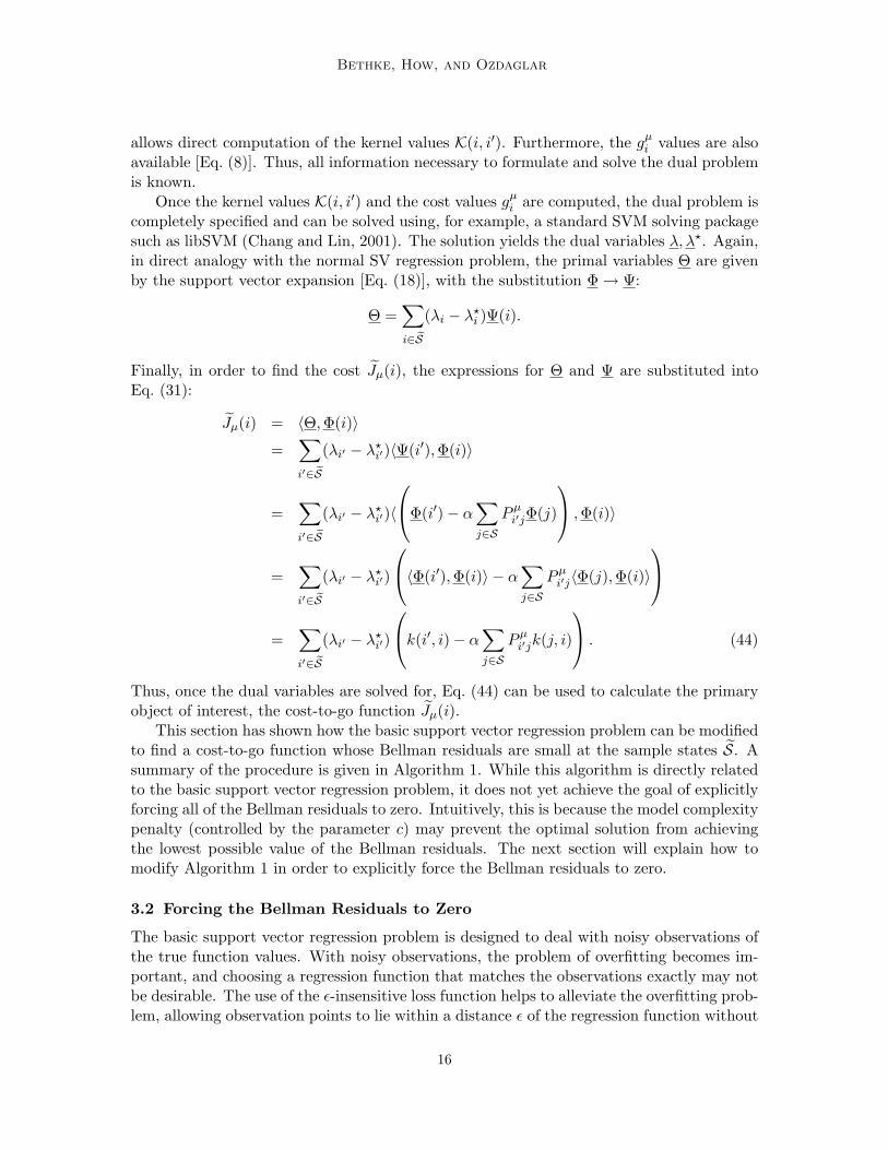
Thus, once the dual variables are solved for, Eq. (44) can be used to calculate the primaryobject of interest, the cost-to-go function Jµ(i).
This section has shown how the basic support vector regression problem can be modifiedto find a cost-to-go function whose Bellman residuals are small at the sample states S. Asummary of the procedure is given in Algorithm 1. While this algorithm is directly relatedto the basic support vector regression problem, it does not yet achieve the goal of explicitlyforcing all of the Bellman residuals to zero. Intuitively, this is because the model complexitypenalty (controlled by the parameter c) may prevent the optimal solution from achievingthe lowest possible value of the Bellman residuals. The next section will explain how tomodify Algorithm 1 in order to explicitly force the Bellman residuals to zero.
3.2 Forcing the Bellman Residuals to Zero
The basic support vector regression problem is designed to deal with noisy observations ofthe true function values. With noisy observations, the problem of overfitting becomes im-portant, and choosing a regression function that matches the observations exactly may notbe desirable. The use of the ε-insensitive loss function helps to alleviate the overfitting prob-lem, allowing observation points to lie within a distance ε of the regression function without
16
Kernel-Based RL Using Bellman Error Elimination
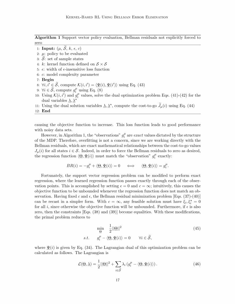
Algorithm 1 Support vector policy evaluation, Bellman residuals not explicitly forced tozero1: Input: (µ, S, k, ε, c)2: µ: policy to be evaluated3: S: set of sample states4: k: kernel function defined on S × S5: ε: width of ε-insensitive loss function6: c: model complexity parameter7: Begin8: ∀i, i′ ∈ S, compute K(i, i′) = 〈Ψ(i),Ψ(i′)〉 using Eq. (43)9: ∀i ∈ S, compute gµ
i using Eq. (8)10: Using K(i, i′) and gµ
i values, solve the dual optimization problem Eqs. (41)-(42) for thedual variables λ, λ?
11: Using the dual solution variables λ, λ?, compute the cost-to-go Jµ(i) using Eq. (44)12: End
causing the objective function to increase. This loss function leads to good performancewith noisy data sets.
However, in Algorithm 1, the “observations” gµi are exact values dictated by the structure
of the MDP. Therefore, overfitting is not a concern, since we are working directly with theBellman residuals, which are exact mathematical relationships between the cost-to-go valuesJµ(i) for all states i ∈ S. Indeed, in order to force the Bellman residuals to zero as desired,the regression function 〈Θ,Ψ(i)〉 must match the “observation” gµ
i exactly:
BR(i) = −gµi + 〈Θ,Ψ(i)〉 = 0 ⇐⇒ 〈Θ,Ψ(i)〉 = gµ
i .
Fortunately, the support vector regression problem can be modified to perform exactregression, where the learned regression function passes exactly through each of the obser-vation points. This is accomplished by setting ε = 0 and c =∞; intuitively, this causes theobjective function to be unbounded whenever the regression function does not match an ob-servation. Having fixed c and ε, the Bellman residual minimization problem [Eqs. (37)-(40)]can be recast in a simpler form. With c = ∞, any feasible solution must have ξi, ξ
?i = 0
for all i, since otherwise the objective function will be unbounded. Furthermore, if ε is alsozero, then the constraints [Eqs. (38) and (39)] become equalities. With these modifications,the primal problem reduces to
minΘ
12||Θ||2 (45)
s.t. gµi − 〈Θ,Ψ(i)〉 = 0 ∀i ∈ S,
where Ψ(i) is given by Eq. (34). The Lagrangian dual of this optimization problem can becalculated as follows. The Lagrangian is
L(Θ, λ) =12||Θ||2 +
∑i∈ eS
λi (gµi − 〈Θ,Ψ(i)〉) . (46)
17
Bethke, How, and Ozdaglar
Maximizing L(Θ, λ) with respect to Θ is accomplished by setting the corresponding partialderivative to zero:
∂L∂Θ
= Θ−∑i∈ eS
λiΨ(i) = 0,
and thereforeΘ =
∑i∈ eS
λiΨ(i). (47)
As a result, the cost function Jµ(i) [Eq. (31)] is given by
Jµ(i) = 〈Θ,Φ(i)〉=
∑i′∈ eS
λi′〈Ψ(i′),Φ(i) 〉
=∑i′∈ eS
λi′
k(i′, i)− α∑j∈S
Pµi′jk(j, i)
. (48)
Finally, substituting Eq. (47) into Eq. (46) and maximizing with respect to λ gives the dualproblem:
maxλ−1
2
∑i,i′∈ eS
λiλi′〈Ψ(i),Ψ(i′)〉+∑i∈ eS
λigµi .
This can also be written in vector form as
maxλ−1
2λT Kλ + λT gµ, (49)
whereKii′ = 〈Ψ(i),Ψ(i′)〉 = K(i, i′)
is the Gram matrix of the kernel K (this matrix is calculated using Eq. (43)). Note that theproblem is just an unconstrained maximization of a quadratic form. Since by assumptionthe base kernel k is nondegenerate, Theorem 2 implies that the associated Bellman kernelK is nondegenerate also. Therefore, the Gram matrix K is full-rank and strictly positivedefinite, so the quadratic form has a unique maximum. The solution is found analyticallyby setting the derivative of the objective with respect to λ to zero, which yields
Kλ = gµ. (50)
Note the important fact that the dimension of this linear system is ns = |S|, the number ofsampled states.
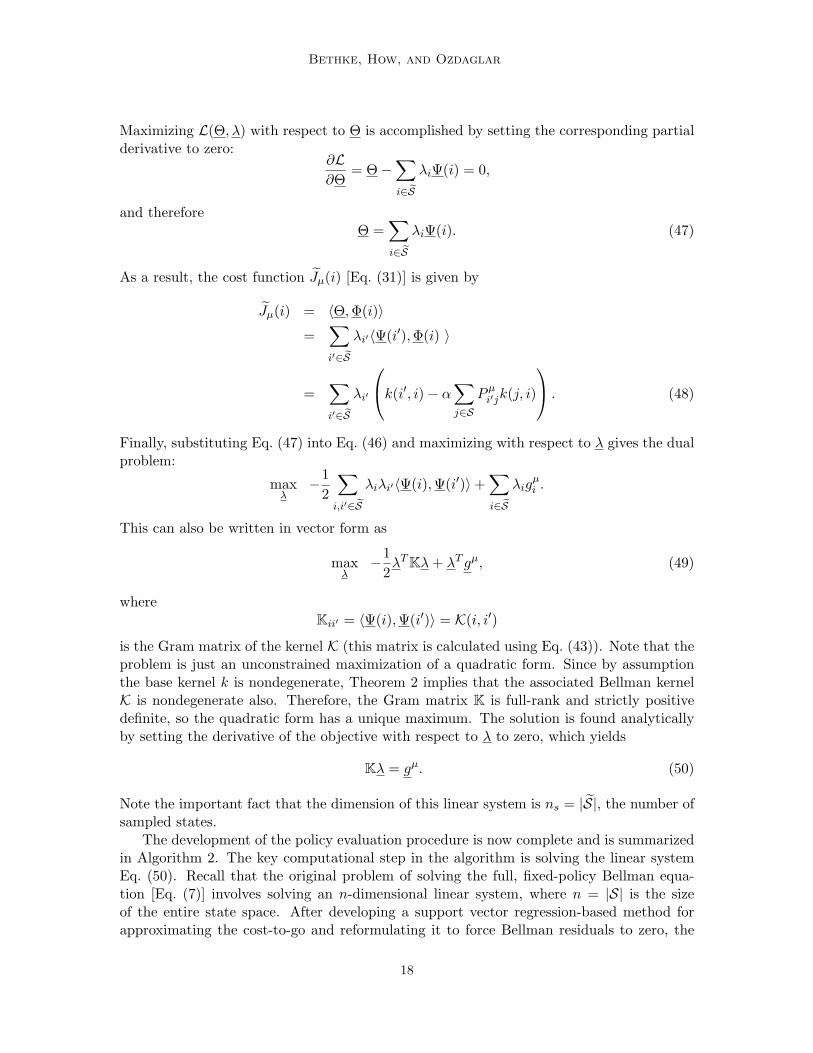
The development of the policy evaluation procedure is now complete and is summarizedin Algorithm 2. The key computational step in the algorithm is solving the linear systemEq. (50). Recall that the original problem of solving the full, fixed-policy Bellman equa-tion [Eq. (7)] involves solving an n-dimensional linear system, where n = |S| is the sizeof the entire state space. After developing a support vector regression-based method forapproximating the cost-to-go and reformulating it to force Bellman residuals to zero, the
18
Kernel-Based RL Using Bellman Error Elimination
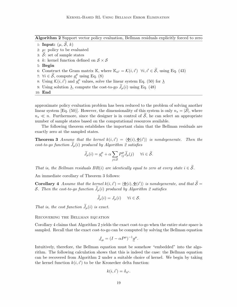
Algorithm 2 Support vector policy evaluation, Bellman residuals explicitly forced to zero
1: Input: (µ, S, k)2: µ: policy to be evaluated3: S: set of sample states4: k: kernel function defined on S × S5: Begin6: Construct the Gram matrix K, where Kii′ = K(i, i′) ∀i, i′ ∈ S, using Eq. (43)7: ∀i ∈ S, compute gµ
i using Eq. (8)8: Using K(i, i′) and gµ
i values, solve the linear system Eq. (50) for λ
9: Using solution λ, compute the cost-to-go Jµ(i) using Eq. (48)10: End
approximate policy evaluation problem has been reduced to the problem of solving anotherlinear system [Eq. (50)]. However, the dimensionality of this system is only ns = |S|, wherens n. Furthermore, since the designer is in control of S, he can select an appropriatenumber of sample states based on the computational resources available.
The following theorem establishes the important claim that the Bellman residuals areexactly zero at the sampled states.
Theorem 3 Assume that the kernel k(i, i′) = 〈Φ(i),Φ(i′)〉 is nondegenerate. Then thecost-to-go function Jµ(i) produced by Algorithm 2 satisfies
Jµ(i) = gµi + α
∑j∈S
Pµij Jµ(j) ∀i ∈ S.
That is, the Bellman residuals BR(i) are identically equal to zero at every state i ∈ S.
An immediate corollary of Theorem 3 follows:
Corollary 4 Assume that the kernel k(i, i′) = 〈Φ(i),Φ(i′)〉 is nondegenerate, and that S =S. Then the cost-to-go function Jµ(i) produced by Algorithm 2 satisfies
Jµ(i) = Jµ(i) ∀i ∈ S.
That is, the cost function Jµ(i) is exact.
Recovering the Bellman equation
Corollary 4 claims that Algorithm 2 yields the exact cost-to-go when the entire state space issampled. Recall that the exact cost-to-go can be computed by solving the Bellman equation
Jµ = (I − αPµ)−1gµ.
Intuitively, therefore, the Bellman equation must be somehow “embedded” into the algo-rithm. The following calculation shows that this is indeed the case: the Bellman equationcan be recovered from Algorithm 2 under a suitable choice of kernel. We begin by takingthe kernel function k(i, i′) to be the Kronecker delta function:
k(i, i′) = δii′ .
19
Bethke, How, and Ozdaglar
This kernel is nondegenerate, since its Gram matrix is always the identity matrix, which isclearly positive definite. Furthermore, we take S = S, so that both conditions of Corollary 4are met. Now, notice that with this choice of kernel, the associated Bellman kernel [Eq. (43)]is
K(i, i′) = δii′ − α∑j∈S
(Pµ
i′jδij + Pµijδi′j
)+ α2
∑j,j′∈S
PµijP
µi′j′δjj′
= δii′ − α(Pµ
i′i + Pµii′)
+ α2∑j∈S
PµijP
µi′j . (51)
Line 6 in Algorithm 2 computes the Gram matrix K of the associated Bellman kernel.A straightforward calculation shows that, with the associated Bellman kernel given byEq. (51), the Gram matrix is
K = (I − αPµ)2.
Line 7 simply constructs the vector gµ, and Line 8 computes λ, which is given by
λ = K−1gµ = (I − αPµ)−2gµ.
Once λ is known, the cost function Jµ(i) is computed in Line 9:
Jµ(i) =∑i′∈S
λi′
δi′i − α∑j∈S
Pµi′jδji
= λi − α
∑i′∈S
λi′Pµi′i.
Expressed as a vector, this cost function can now be written as
Jµ = λ− αPµλ
= (I − αPµ)λ= (I − αPµ)(I − αPµ)−2gµ
= (I − αPµ)−1gµ
= Jµ.
Thus, we see that for the choice of kernel k(i, i′) = δii′ and sample states S = S, Algorithm 2effectively reduces to solving the Bellman equation directly. Of course, if the Bellmanequation could be solved directly for a particular problem, it would make little sense touse an approximation algorithm of any kind. Furthermore, the Kronecker delta is a poorpractical choice for the kernel, since the kernel is zero everywhere except at i = i′; we use ithere only to illustrate the properties of the algorithm. The real value of the algorithm arisesbecause the main results - namely, that the Bellman residuals are identically zero at thesample states - are valid for any nondegenerate kernel function and any set of sample statesS ⊆ S. This permits the use of “smoothing” kernels that enable the computed cost functionto generalize to states that were not sampled, which is a major goal of any reinforcementlearning algorithm. Thus, in the more realistic case where solving the Bellman equation
20
Kernel-Based RL Using Bellman Error Elimination
Algorithm 3 BRE(SV)
1: Input: (µ0, S, k)2: µ0: initial policy3: S: set of sample states4: k: kernel function defined on S × S5: Begin6: µ← µ0
7: loop8: Jµ(i)← ALGORITHM 2(µ, S, k) Policy evaluation9: µ(i)← arg minu
∑j∈S Pij(u)
(g(i, u) + αJµ(j)
)Policy improvement
10: end loop11: End
directly is not practical, Algorithm 2 (with a smaller set of sample states and a suitablekernel function) becomes a way of effectively reducing the dimensionality of the Bellmanequation to a tractable size while preserving the character of the original equation.
The associated Bellman kernel [Eq. (43)] plays a central role in the work developed thusfar; it is this kernel and its associated feature mapping Ψ [Eq. (34)] that effectively allowthe Bellman equation to be embedded into the algorithms, and consequently to ensure thatthe Bellman residuals at the sampled states are zero. This idea will be developed furtherin Section 4.
3.3 BRE(SV), A Full Policy Iteration Algorithm
Algorithm 2 shows how to construct a cost-to-go approximation Jµ(·) of a fixed policy µ
such that the Bellman residuals are exactly zero at the sample states S. This section nowpresents BRE(SV) (Algorithm 3), a full policy iteration algorithm that uses Algorithm 2 inthe policy evaluation step.
The following corollary to Theorem 3 establishes that BRE(SV) reduces to exact policyiteration when the entire state space is sampled:
Corollary 5 Assume that the kernel k(i, i′) = 〈Φ(i),Φ(i′)〉 is nondegenerate, and that S =S. Then BRE(SV) is equivalent to exact policy iteration.
This result is encouraging, since it is well known that exact policy iteration converges tothe optimal policy in a finite number of steps (Bertsekas, 2007).
3.4 Computational Results
BRE(SV) was implemented on the well-known “mountain car problem” (Sutton and Barto,1998; Rasmussen and Kuss, 2004) to evaluate its performance. In this problem, a unit mass,frictionless car moves along a hilly landscape whose height H(x) is described by
H(x) =
x2 + x if x < 0
x√1+5x2
if x ≥ 0.
21
Bethke, How, and Ozdaglar
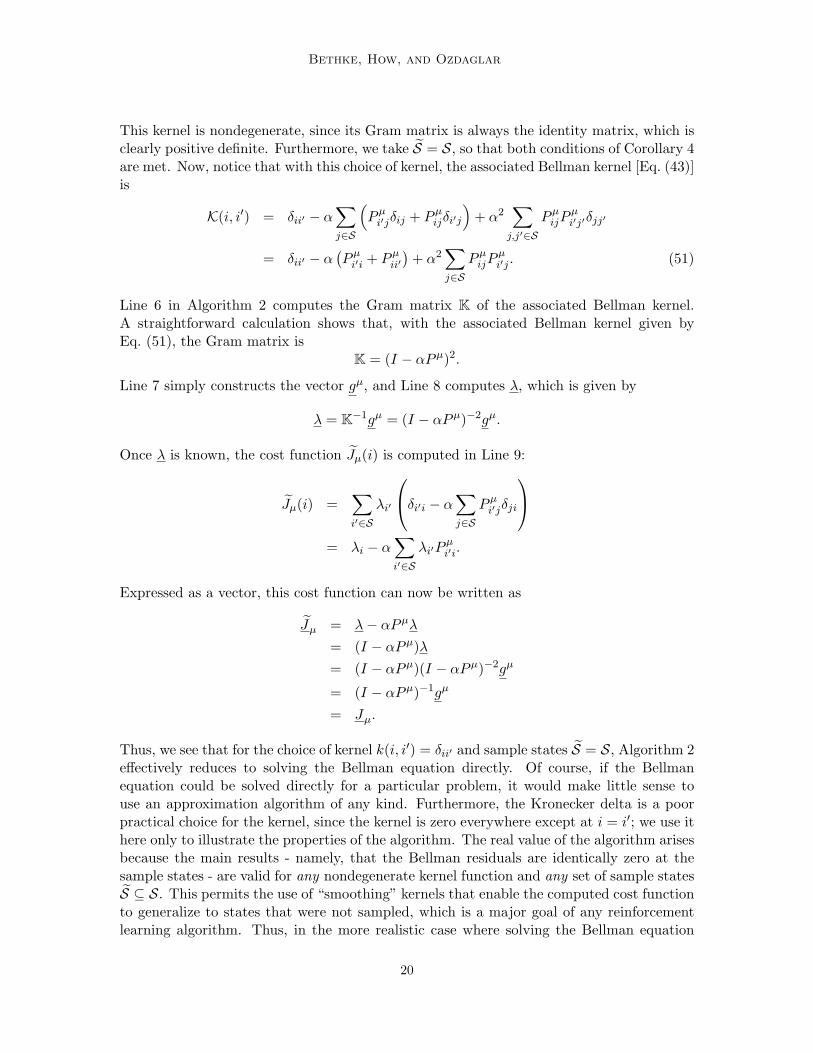
Figure 1: System response under the optimal policy (dashed line) and the policy computedby BRE(SV) after 3 iterations (solid line).
The system state is given by (x, x) (the horizontal position and velocity of the car). Ahorizontal control force −4 ≤ u ≤ 4 can be applied to the car, and the goal is to drive thecar from its starting location x = −0.5 to the “parking area” 0.5 ≤ x ≤ 0.7 as quickly aspossible. Since the car is also acted upon by gravitational acceleration g = 9.8, the totalhorizontal acceleration of the car, x, is given by
x =u− gH ′(x)1 + H ′(x)2
,
where H ′(x) denotes the derivative dH(x)dx . The problem is challenging because the car is
underpowered: it cannot simply drive up the steep slope. Rather, it must use the featuresof the landscape to build momentum and eventually escape the steep valley centered atx = −0.5. The system response under the optimal policy (computed using value iteration)is shown as the dashed line in Figure 1; notice that the car initially moves away from theparking area before reaching it at time t = 14.
In order to apply the support vector policy iteration algorithm, an evenly spaced 9x9grid of sample states,
S = (x, x) | x = −1.0,−0.75, . . . , 0.75, 1.0x = −2.0,−1.5, . . . , 1.5, 2.0
was chosen. Furthermore, a radial basis function kernel, with differing length-scales for thex and x axes in the state space, was used:
k((x1, x1), (x2, x2)) = exp (−(x1 − x2)2/(0.25)2 − (x1 − x2)2/(0.40)2).
22
Kernel-Based RL Using Bellman Error Elimination
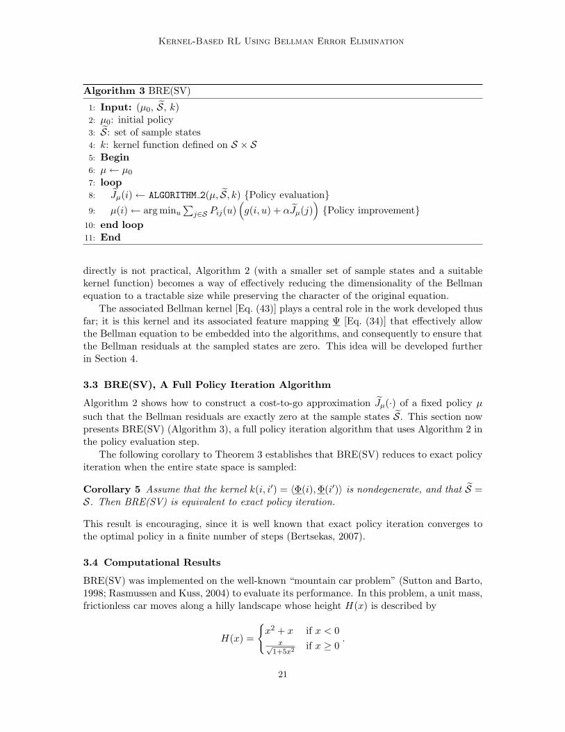
Figure 2: From left to right: Approximate cost-to-go computed by BRE(SV) for iterations1, 2 , and 3; exact cost-to-go computed using value iteration.
BRE(SV) was executed, resulting in a sequence of policies (and associated cost functions)that converged after three iterations. The sequence of cost functions is shown in Figure 2along with the optimal cost function for comparison. Of course, the main objective isto learn a policy that is similar to the optimal one. The solid line in Figure 1 shows thesystem response under the approximate policy generated by the algorithm after 3 iterations.Notice that the qualitative behavior is the same as the optimal policy; that is, the car firstaccelerates away from the parking area to gain momentum. The approximate policy arrivesat the parking area at t = 17, only 3 time steps slower than the optimal policy.
BRE(SV) was derived starting from the viewpoint of the standard support vector re-gression framework. The theorems of this section have established several advantageoustheoretical properties of the approach, and furthermore, the results from the mountain carexample problem demonstrate that BRE(SV) produces a high-quality cost approximationand policy. The example problem highlights two interesting questions:
1. The scaling parameters (0.25 and 0.40) used in the squared exponential kernel werefound, in this case, by carrying out numerical experiments to see which values fitthe data best. Is it possible to design a BRE algorithm that can learn these valuesautomatically as it runs?
2. Is it possible to provide error bounds on the learned cost-to-go function for the non-sampled states?
Fortunately, the answer to both of these questions is yes. In the next section, we showhow the key ideas in BRE(SV) can be extended to a more general framework, which allowsBRE to be performed using any kernel-based regression technique. This analysis will resultin a deeper understanding of the approach and also enable the development of a BREalgorithm based on Gaussian process regression, BRE(GP), that preserves all the advantagesof BRE(SV) while addressing these two questions.
23
Bethke, How, and Ozdaglar
4. A General BRE Framework
Building on the ideas and intuition presented in the development of BRE(SV), we nowseek to understand how that algorithm can be generalized. To begin, it is useful to viewkernel-based regression techniques, such as support vector regression and Gaussian pro-cess regression, as algorithms that search over a reproducing kernel Hilbert space for aregression function solution. In particular, given a kernel k and a set of training dataD = (x1, y1), . . . , (xn, yn), these kernel-based regression techniques find a solution of thestandard form
f(x) = 〈Θ,Φ(x)〉,
where Φ is the feature mapping of the kernel k. The solution f belongs to the RKHS Hk
of the kernel k:f(·) ∈ Hk.
Broadly speaking, the various kernel-based regression techniques are differentiated by howthey choose the weighting element Θ, which in turn uniquely specifies the solution f fromthe space of functions Hk.
In the BRE(SV) algorithm developed in the previous section, the kernel k and its as-sociated Bellman kernel K play a central role. Recall the relationship between these twokernels:
k(i, i′) = 〈Φ(i),Φ(i′)〉 (52)
Ψ(i) = Φ(i)− α∑j∈S
PµijΦ(j) (53)
K(i, i′) = 〈Ψ(i),Ψ(i′)〉. (54)
By the uniqueness property of Section 2.4, each of the kernels is associated with its own,unique RHKS, denoted by Hk and HK, respectively. In this section, we explore someproperties of these RKHSs, and use the properties to develop a general BRE framework.In particular, it is shown that Hk corresponds to the space of possible cost-to-go functions,while HK corresponds to the space of Bellman residual functions. We explain how theproblem of performing BRE is equivalent to solving a simple regression problem in HK inorder to find a Bellman residual function with the desired property of being zero at thesampled states S. This regression problem can be solved using any kernel-based regressiontechnique. Furthermore, an invertible linear mapping between elements of Hk and HK isconstructed. This mapping can be used to find the corresponding cost-to-go function oncethe Bellman residual function is found.
4.1 The Cost Space Hk
The goal of any approximate policy iteration algorithm, including our BRE methods, isto learn an approximation Jµ(·) to the true cost-to-go function Jµ(·). As discussed, if akernel-based regression algorithm, with kernel k(i, i′) = 〈Φ(i),Φ(i′)〉, is used to find theapproximate cost function Jµ(·), then this function is an element of Hk and takes thestandard form
Jµ(i) = 〈Θ,Φ(i)〉.
24
Kernel-Based RL Using Bellman Error Elimination
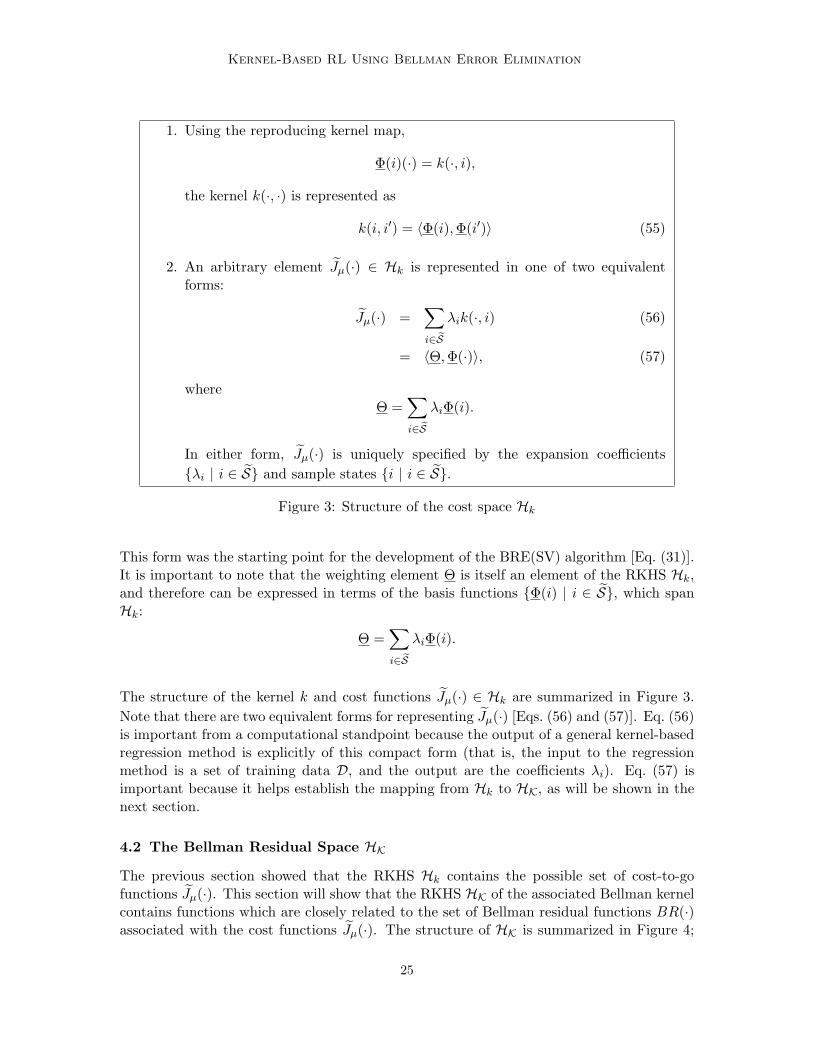
1. Using the reproducing kernel map,
Φ(i)(·) = k(·, i),
the kernel k(·, ·) is represented as
k(i, i′) = 〈Φ(i),Φ(i′)〉 (55)
2. An arbitrary element Jµ(·) ∈ Hk is represented in one of two equivalentforms:
Jµ(·) =∑i∈ eS
λik(·, i) (56)
= 〈Θ,Φ(·)〉, (57)
whereΘ =
∑i∈ eS
λiΦ(i).
In either form, Jµ(·) is uniquely specified by the expansion coefficientsλi | i ∈ S and sample states i | i ∈ S.
Figure 3: Structure of the cost space Hk
This form was the starting point for the development of the BRE(SV) algorithm [Eq. (31)].It is important to note that the weighting element Θ is itself an element of the RKHS Hk,and therefore can be expressed in terms of the basis functions Φ(i) | i ∈ S, which spanHk:
Θ =∑i∈ eS
λiΦ(i).
The structure of the kernel k and cost functions Jµ(·) ∈ Hk are summarized in Figure 3.Note that there are two equivalent forms for representing Jµ(·) [Eqs. (56) and (57)]. Eq. (56)is important from a computational standpoint because the output of a general kernel-basedregression method is explicitly of this compact form (that is, the input to the regressionmethod is a set of training data D, and the output are the coefficients λi). Eq. (57) isimportant because it helps establish the mapping from Hk to HK, as will be shown in thenext section.
4.2 The Bellman Residual Space HK
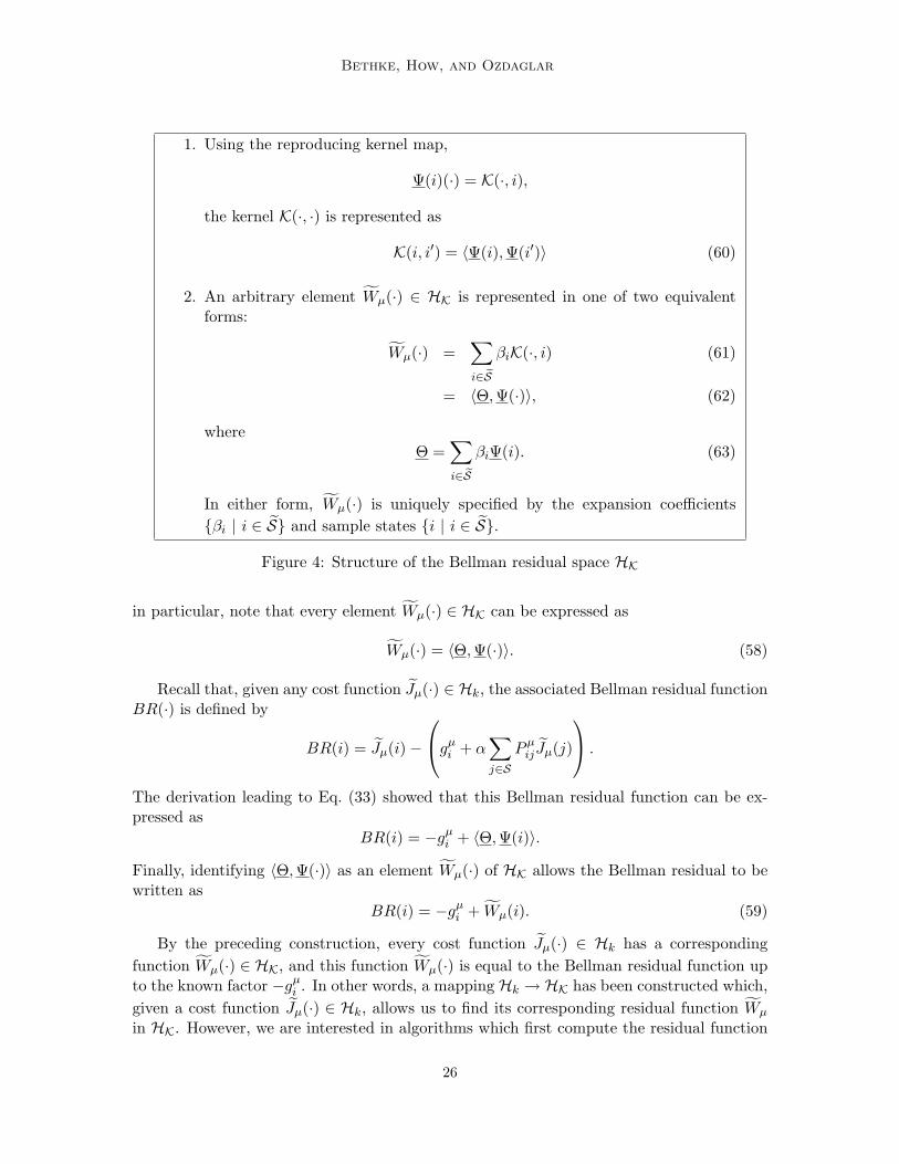
The previous section showed that the RKHS Hk contains the possible set of cost-to-gofunctions Jµ(·). This section will show that the RKHS HK of the associated Bellman kernelcontains functions which are closely related to the set of Bellman residual functions BR(·)associated with the cost functions Jµ(·). The structure of HK is summarized in Figure 4;
25
Bethke, How, and Ozdaglar
1. Using the reproducing kernel map,
Ψ(i)(·) = K(·, i),
the kernel K(·, ·) is represented as
K(i, i′) = 〈Ψ(i),Ψ(i′)〉 (60)
2. An arbitrary element Wµ(·) ∈ HK is represented in one of two equivalentforms:
Wµ(·) =∑i∈ eS
βiK(·, i) (61)
= 〈Θ,Ψ(·)〉, (62)
whereΘ =
∑i∈ eS
βiΨ(i). (63)
In either form, Wµ(·) is uniquely specified by the expansion coefficientsβi | i ∈ S and sample states i | i ∈ S.
Figure 4: Structure of the Bellman residual space HK
in particular, note that every element Wµ(·) ∈ HK can be expressed as
Wµ(·) = 〈Θ,Ψ(·)〉. (58)
Recall that, given any cost function Jµ(·) ∈ Hk, the associated Bellman residual functionBR(·) is defined by
BR(i) = Jµ(i)−
gµi + α
∑j∈S
Pµij Jµ(j)
.
The derivation leading to Eq. (33) showed that this Bellman residual function can be ex-pressed as
BR(i) = −gµi + 〈Θ,Ψ(i)〉.
Finally, identifying 〈Θ,Ψ(·)〉 as an element Wµ(·) of HK allows the Bellman residual to bewritten as
BR(i) = −gµi + Wµ(i). (59)
By the preceding construction, every cost function Jµ(·) ∈ Hk has a correspondingfunction Wµ(·) ∈ HK, and this function Wµ(·) is equal to the Bellman residual function upto the known factor −gµ
i . In other words, a mapping Hk → HK has been constructed which,given a cost function Jµ(·) ∈ Hk, allows us to find its corresponding residual function Wµ
in HK. However, we are interested in algorithms which first compute the residual function
26
Kernel-Based RL Using Bellman Error Elimination
and then find the corresponding cost function. Therefore, the mapping must be shown tobe invertible. The following theorem establishes this important property:
Theorem 6 Assume that the kernel k(i, i′) = 〈Φ(i),Φ(i′)〉 is nondegenerate. Then thereexists a linear, invertible mapping A from Hk, the RKHS of k, to HK, the RKHS of theassociated Bellman kernel K:
A : Hk → HKAJµ(·) = Wµ(·).
Furthermore, if an element Jµ(·) ∈ Hk is given by
Jµ(·) = 〈Θ,Φ(·)〉,
then the corresponding element Wµ(·) ∈ HK is given by
Wµ(·) = 〈Θ,Ψ(·)〉,
and vice versa:
Jµ(·) = 〈Θ,Φ(·)〉m (64)
Wµ(·) = 〈Θ,Ψ(·)〉.
The mapping A of Theorem 6 allows us to design BRE algorithms that find the weightelement Θ of the desired residual function Wµ(·) ∈ HK and then map the result back to Hk
in order to find the associated cost function Jµ(·) (using Eq. (64)).The objective of the BRE algorithms is to force the Bellman residuals BR(i) to zero at
the sample states S:BR(i) = 0 ∀i ∈ S. (65)
Now, using Eq. (59), we see that Eq. (65) is equivalent to
Wµ(i) = gµi ∀i ∈ S. (66)
We have now succeeded in reducing the BRE problem to a straightforward regression prob-lem in HK: the task is to find a function Wµ(i) ∈ HK that satisfies Eq. (66). The trainingdata of the regression problem is given by
D = (i, gµi ) | i ∈ S.
Notice that the training data is readily available, since by assumption the sample states Sare given, and the stage costs gµ
i are obtained directly from the MDP specification.
27
Bethke, How, and Ozdaglar
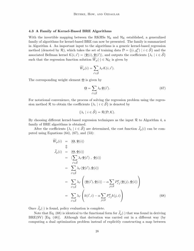
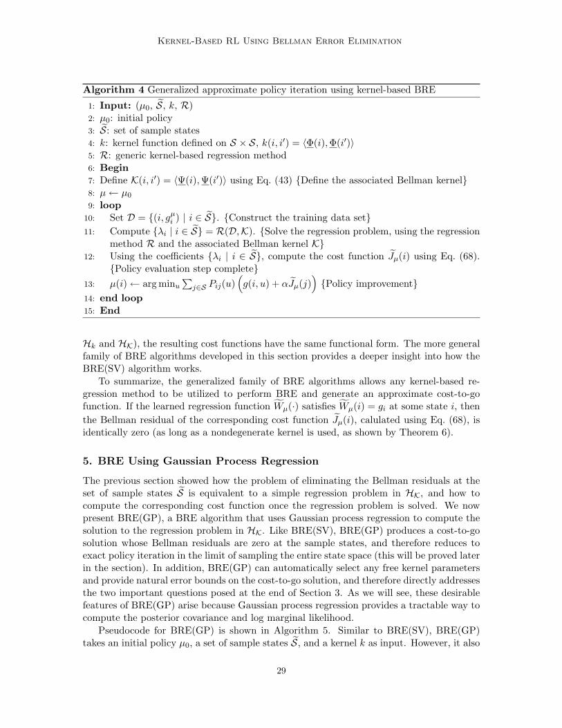
4.3 A Family of Kernel-Based BRE Algorithms
With the invertible mapping between the RKHSs Hk and HK established, a generalizedfamily of algorithms for kernel-based BRE can now be presented. The family is summarizedin Algorithm 4. An important input to the algorithms is a generic kernel-based regressionmethod (denoted by R), which takes the set of training data D = (i, gµ
i ) | i ∈ S and theassociated Bellman kernel K(i, i′) = 〈Ψ(i),Ψ(i′)〉, and outputs the coefficients λi | i ∈ Ssuch that the regression function solution Wµ(·) ∈ HK is given by
Wµ(i) =∑i′∈ eS
λi′K(i, i′).
The corresponding weight element Θ is given by
Θ =∑i′∈ eS
λi′Ψ(i′). (67)
For notational convenience, the process of solving the regression problem using the regres-sion method R to obtain the coefficients λi | i ∈ S is denoted by
λi | i ∈ S = R(D,K).
By choosing different kernel-based regression techniques as the input R to Algorithm 4, afamily of BRE algorithms is obtained.
After the coefficients λi | i ∈ S are determined, the cost function Jµ(i) can be com-puted using Equations (64), (67), and (53):
Wµ(i) = 〈Θ,Ψ(i)〉m
Jµ(i) = 〈Θ,Φ(i)〉= 〈
∑i′∈ eS
λi′Ψ(i′) , Φ(i)〉
=∑i′∈ eS
λi′〈Ψ(i′),Φ(i)〉
=∑i′∈ eS
λi′
〈Φ(i′),Φ(i)〉 − α∑j∈S
Pµi′j〈Φ(j),Φ(i)〉
=
∑i′∈ eS
λi′
k(i′, i)− α∑j∈S
Pµi′jk(j, i)
(68)
Once Jµ(·) is found, policy evaluation is complete.Note that Eq. (68) is identical to the functional form for Jµ(·) that was found in deriving
BRE(SV) [Eq. (48)]. Although that derivation was carried out in a different way (bycomputing a dual optimization problem instead of explicitly constructing a map between
28
Kernel-Based RL Using Bellman Error Elimination
Algorithm 4 Generalized approximate policy iteration using kernel-based BRE
1: Input: (µ0, S, k, R)2: µ0: initial policy3: S: set of sample states4: k: kernel function defined on S × S, k(i, i′) = 〈Φ(i),Φ(i′)〉5: R: generic kernel-based regression method6: Begin7: Define K(i, i′) = 〈Ψ(i),Ψ(i′)〉 using Eq. (43) Define the associated Bellman kernel8: µ← µ0
9: loop10: Set D = (i, gµ
i ) | i ∈ S. Construct the training data set11: Compute λi | i ∈ S = R(D,K). Solve the regression problem, using the regression
method R and the associated Bellman kernel K12: Using the coefficients λi | i ∈ S, compute the cost function Jµ(i) using Eq. (68).
Policy evaluation step complete13: µ(i)← arg minu
∑j∈S Pij(u)
(g(i, u) + αJµ(j)
)Policy improvement
14: end loop15: End
Hk and HK), the resulting cost functions have the same functional form. The more generalfamily of BRE algorithms developed in this section provides a deeper insight into how theBRE(SV) algorithm works.
To summarize, the generalized family of BRE algorithms allows any kernel-based re-gression method to be utilized to perform BRE and generate an approximate cost-to-gofunction. If the learned regression function Wµ(·) satisfies Wµ(i) = gi at some state i, thenthe Bellman residual of the corresponding cost function Jµ(i), calulated using Eq. (68), isidentically zero (as long as a nondegenerate kernel is used, as shown by Theorem 6).
5. BRE Using Gaussian Process Regression
The previous section showed how the problem of eliminating the Bellman residuals at theset of sample states S is equivalent to a simple regression problem in HK, and how tocompute the corresponding cost function once the regression problem is solved. We nowpresent BRE(GP), a BRE algorithm that uses Gaussian process regression to compute thesolution to the regression problem in HK. Like BRE(SV), BRE(GP) produces a cost-to-gosolution whose Bellman residuals are zero at the sample states, and therefore reduces toexact policy iteration in the limit of sampling the entire state space (this will be proved laterin the section). In addition, BRE(GP) can automatically select any free kernel parametersand provide natural error bounds on the cost-to-go solution, and therefore directly addressesthe two important questions posed at the end of Section 3. As we will see, these desirablefeatures of BRE(GP) arise because Gaussian process regression provides a tractable way tocompute the posterior covariance and log marginal likelihood.
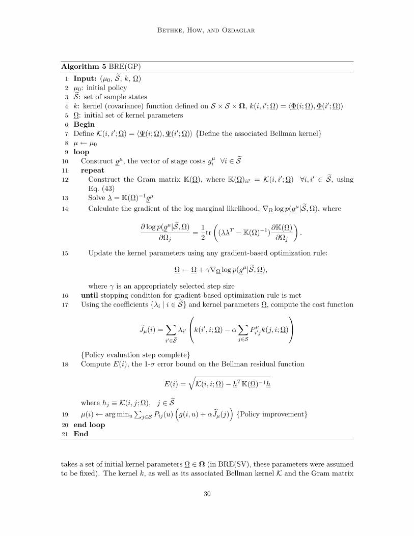
Pseudocode for BRE(GP) is shown in Algorithm 5. Similar to BRE(SV), BRE(GP)takes an initial policy µ0, a set of sample states S, and a kernel k as input. However, it also
29
Bethke, How, and Ozdaglar
Algorithm 5 BRE(GP)
1: Input: (µ0, S, k, Ω)2: µ0: initial policy3: S: set of sample states4: k: kernel (covariance) function defined on S × S ×Ω, k(i, i′; Ω) = 〈Φ(i; Ω),Φ(i′; Ω)〉5: Ω: initial set of kernel parameters6: Begin7: Define K(i, i′; Ω) = 〈Ψ(i; Ω),Ψ(i′; Ω)〉 Define the associated Bellman kernel8: µ← µ0
9: loop10: Construct gµ, the vector of stage costs gµ
i ∀i ∈ S11: repeat12: Construct the Gram matrix K(Ω), where K(Ω)ii′ = K(i, i′; Ω) ∀i, i′ ∈ S, using
Eq. (43)13: Solve λ = K(Ω)−1gµ
14: Calculate the gradient of the log marginal likelihood, ∇Ω log p(gµ|S,Ω), where
∂ log p(gµ|S,Ω)∂Ωj
=12tr(
(λλT −K(Ω)−1)∂K(Ω)∂Ωj
).
15: Update the kernel parameters using any gradient-based optimization rule:
Ω← Ω + γ∇Ω log p(gµ|S,Ω),
where γ is an appropriately selected step size16: until stopping condition for gradient-based optimization rule is met17: Using the coefficients λi | i ∈ S and kernel parameters Ω, compute the cost function
Jµ(i) =∑i′∈ eS
λi′
k(i′, i; Ω)− α∑j∈S
Pµi′jk(j, i; Ω)
Policy evaluation step complete
18: Compute E(i), the 1-σ error bound on the Bellman residual function
E(i) =√K(i, i; Ω)− hT K(Ω)−1h
where hj ≡ K(i, j; Ω), j ∈ S19: µ(i)← arg minu
∑j∈S Pij(u)
(g(i, u) + αJµ(j)
)Policy improvement
20: end loop21: End
takes a set of initial kernel parameters Ω ∈ Ω (in BRE(SV), these parameters were assumedto be fixed). The kernel k, as well as its associated Bellman kernel K and the Gram matrix
30
Kernel-Based RL Using Bellman Error Elimination
K all depend on these parameters, and to emphasize this dependence they are written ask(i, i′; Ω), K(i, i′; Ω), and K(Ω), respectively.
The algorithm consists of two nested loops. The inner loop (lines 11-16) is responsiblefor repeatedly solving the regression problem in HK (notice that the target values of theregression problem, the one-stage costs gµ, are computed in line 10) and adjusting the kernelparameters using gradient-based optimization. This process is carried out with the policyfixed, so the kernel parameters are tuned to each policy prior to the policy improvementstage being carried out. Line 13 computes the λ values necessary to compute the meanfunction of the posterior process [Eq. (23)]. Lines 14 and 15 then compute the gradient ofthe log likelihood function, using Eq. (25), and use this gradient information to update thekernel parameters. This process continues until a maximum of the log likelihood functionhas been found.
Once the kernel parameters are optimally adjusted for the current policy µ, the mainbody of the outer loop (lines 17-19) performs three important tasks. First, it computes thecost-to-go solution Jµ(i) using Eq. (68) (rewritten on line 17 to emphasize dependence onΩ). Second, on line 18, it computes the posterior standard deviation E(i) of the Bellmanresidual function. This quantity is computed using the standard result from Gaussianprocess regression for computing the posterior variance [Eq. (22)], and it gives a Bayesianerror bound on the magnitude of the Bellman residual BR(i). This error bound is useful, ofcourse, because the goal is to achieve small Bellman residuals at as many states as possible.Finally, the algorithm carries out a policy improvement step in Line 19.
Note that the log likelihood function is not necessarily guaranteed to be convex, so itmay be possible for the gradient optimization carried out in the inner loop (lines 11-16) toconverge to a local (but not global) maximum. However, by initializing the optimizationprocess at several starting points, it may be possible to decrease the probability of endingup in a local maximum (Rasmussen and Williams, 2006, 5.4).
The following theorems establish the same important properties of BRE(GP) that wereproved earlier for BRE(SV):
Theorem 7 Assume that the kernel k(i, i′; Ω) = 〈Φ(i; Ω),Φ(i′; Ω)〉 is nondegenerate. Thenthe cost-to-go functions Jµ(i) computed by BRE(GP) (on line 17) satisfy
Jµ(i) = gµi + α
∑j∈S
Pµij Jµ(j) ∀i ∈ S.
That is, the Bellman residuals BR(i) are identically zero at every state i ∈ S.
An immediate corollary of Theorem 7 follows:
Corollary 8 Assume that the kernel k(i, i′; Ω) = 〈Φ(i; Ω),Φ(i′; Ω)〉 is nondegenerate, andthat S = S. Then the cost-to-go function Jµ(i) produced by BRE(GP) satisfies
Jµ(i) = Jµ(i) ∀i ∈ S.
That is, the cost function Jµ(i) is exact.
Corollary 9 Assume that the kernel k(i, i′; Ω) = 〈Φ(i; Ω),Φ(i′; Ω)〉 is nondegenerate, andthat S = S. Then BRE(GP) is equivalent to exact policy iteration.
31
Bethke, How, and Ozdaglar
5.1 Computational Complexity
The computational complexity of running BRE(GP) is dominated by steps 12 (constructingthe Gram matrix) and 13 (inverting the Gram matrix). To obtain an expression for thecomputational complexity of the algorithm, first define
ns ≡ |S|
as the number of sample states. Furthermore, define the average branching factor of theMDP, β, as the average number of possible successor states for any state i ∈ S, or equiva-lently, as the average number of terms Pµ
ij that are nonzero for fixed i and µ. Finally, recallthat since K(i, i′) is nondegenerate (as proved earlier), the Gram matrix is positive definiteand symmetric.
Now, each entry of the Gram matrix K(Ω)ii′ is computed using Eq. (43). Using theaverage branching factor defined above, computing a single element of the Gram matrixusing Eq. (43) therefore requires O(β2) operations. Since the Gram matrix is symmetricand of dimension ns × ns, there are ns(ns + 1)/2 unique elements that must be computed.Therefore, the total number of operations to compute the full Gram matrix is
O(β2ns(ns + 1)/2).
Once the Gram matrix is constructed, its inverse must be computed in line 13. Sincethe Gram matrix is positive definite and symmetric, Cholesky decomposition can be used,resulting in a total complexity of
O(n3s)
for line 13. (The results of the Cholesky decomposition computed in line 13 can and shouldbe saved to speed up the calculation of the log marginal likelihood in line 14, which alsorequires the inverse of the Gram matrix). As a result, the total complexity of the BRE(GP)algorithm is
O(n3s + β2ns(ns + 1)/2). (69)
This complexity can be compared with the complexity of exact policy iteration. Recallthat exact policy iteration requires inverting the matrix (I − αPµ) in order to evaluate thepolicy µ:
Jµ = (I − αPµ)−1gµ.
(I − αPµ) is of dimension n× n, where
n = |S|
is the size of the state space. Therefore, the complexity of exact policy iteration is
O(n3). (70)
Comparing Eqs. (69) and (70), notice that both expressions involve cubic terms in ns
and n, respectively. By assumption, the number of sample states is taken to be much smallerthan the total size of the state space (ns n). Furthermore, the average branching factorβ is typically also much smaller than n (and can certainly be no larger than n). Therefore,the computational complexity of BRE(GP) is significantly less than the computationalcomplexity of exact policy iteration.
32
Kernel-Based RL Using Bellman Error Elimination
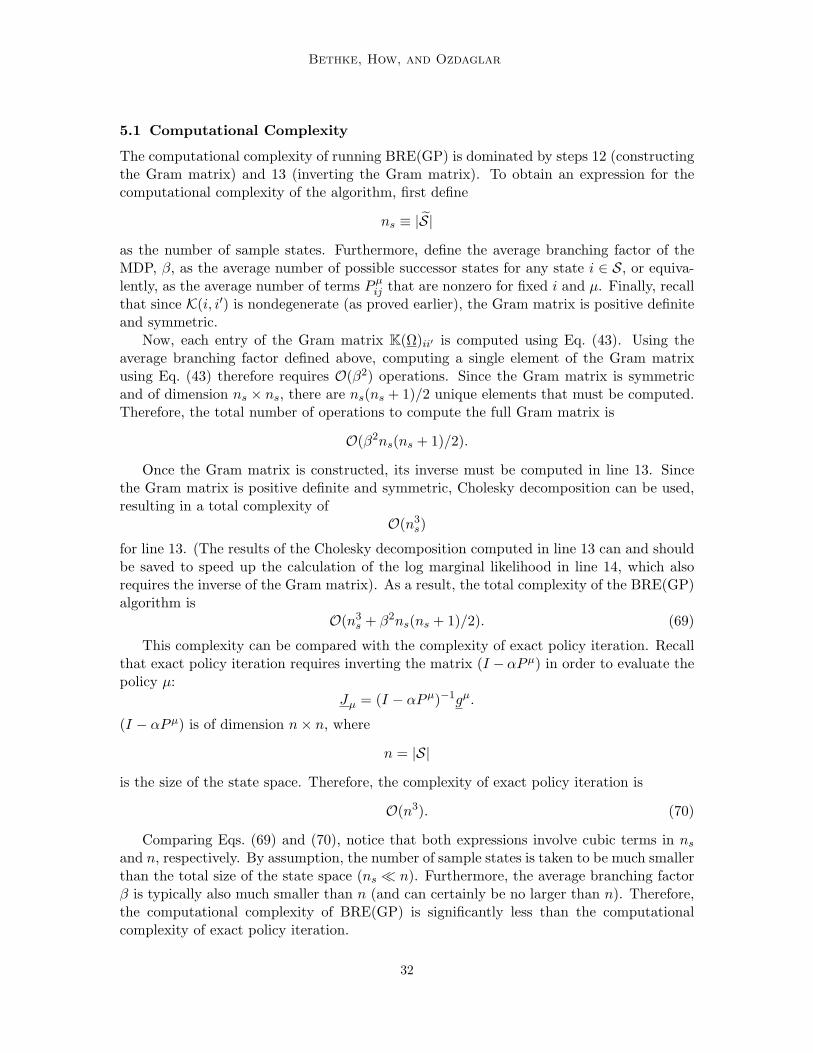
Figure 5: From left to right: Approximate cost-to-go computed by BRE(GP) for iterations1, 2 , and 3; exact cost-to-go computed using value iteration.
5.2 Computational Results
BRE(GP) was implemented on the same mountain car problem examined earlier for BRE(SV).The kernel function employed for these experiments was
k((x1, x1), (x2, x2); Ω) = exp (−(x1 − x2)2/Ω21 − (x1 − x2)2/Ω2
2).
This is the same functional form of the kernel that was used for BRE(SV). However, thelength-scales Ω1 and Ω2 were left as free kernel parameters to be automatically learned bythe BRE(GP) algorithm, in contrast with the BRE(SV) tests, where these values had to bespecified by hand. The parameters were initially set at Ω1 = Ω2 = 10. These values weredeliberately chosen to be far from the empirically chosen values used in the BRE(SV) tests,which were Ω1 = 0.25 and Ω2 = 0.40. Therefore, the test reflected a realistic situation inwhich the parameter values were not initially well-known.
Initially, the same 9x9 grid of sample states as used in the BRE(SV) tests was employedto compare the performance of the two algorithms:
S = (x, x) | x = −1.0,−0.75, . . . , 0.75, 1.0x = −2.0,−1.5, . . . , 1.5, 2.0.
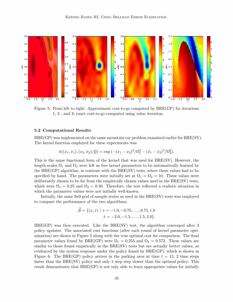
BRE(GP) was then executed. Like the BRE(SV) test, the algorithm converged after 3policy updates. The associated cost functions (after each round of kernel parameter opti-mization) are shown in Figure 5 along with the true optimal cost for comparison. The finalparameter values found by BRE(GP) were Ω1 = 0.253 and Ω2 = 0.572. These values aresimilar to those found empirically in the BRE(SV) tests but are actually better values, asevidenced by the system response under the policy found by BRE(GP), which is shown inFigure 6. The BRE(GP) policy arrives in the parking area at time t = 15, 2 time stepsfaster than the BRE(SV) policy and only 1 step step slower than the optimal policy. Thisresult demonstrates that BRE(GP) is not only able to learn appropriate values for initially
33
Bethke, How, and Ozdaglar
Figure 6: System response under the optimal policy (dashed line) and the policy computedby BRE(GP) after 3 iterations (solid line).
unknown kernel parameters, but also that the resulting policy can be of higher quality thancould be obtained using time-consuming empirical testing.
As discussed, in addition to automatically learning the kernel parameters, BRE(GP)also computes error bounds on the cost-to-go solution. Figure 7 plots the Bellman residualsBR(i), as well as the 2σ error bounds 2E(i) computed in line 18 of the BRE(GP) algorithm.For clarity, the plot is given as a function of x only; x was fixed to zero. The sampled states
(x, 0) | x = −1.0,−0.75, . . . , 0.75, 1.0
are represented by red dots in the figure. Notice that, as expected, the Bellman residuals atthe sampled states are exactly zero. Furthermore, the error bounds computed by BRE(GP),shown as the dashed green lines, do a good job of bounding the Bellman residuals at non-sampled states. Recall that these bounds represent the posterior variance of the Bellmanresiduals. Thus, for the 2σ case shown in the figure, the bounds represent a 95% confidenceinterval, so we expect that 95% of the Bellman residuals should lie within the bounds. Thereare two cases where the residuals lie outside the bounds (at x = 0.45 and x = 0.70), andthere are a total of 81 points in the graph. This leads to an empirical confidence interval of
81− 281
= 97.53%,
which is in excellent agreement with the bounds computed by BRE(GP).A further series of tests were conducted to explore the quality of the policies produced
by BRE(GP) as a function of the number of sample states. In these tests, a uniform
34
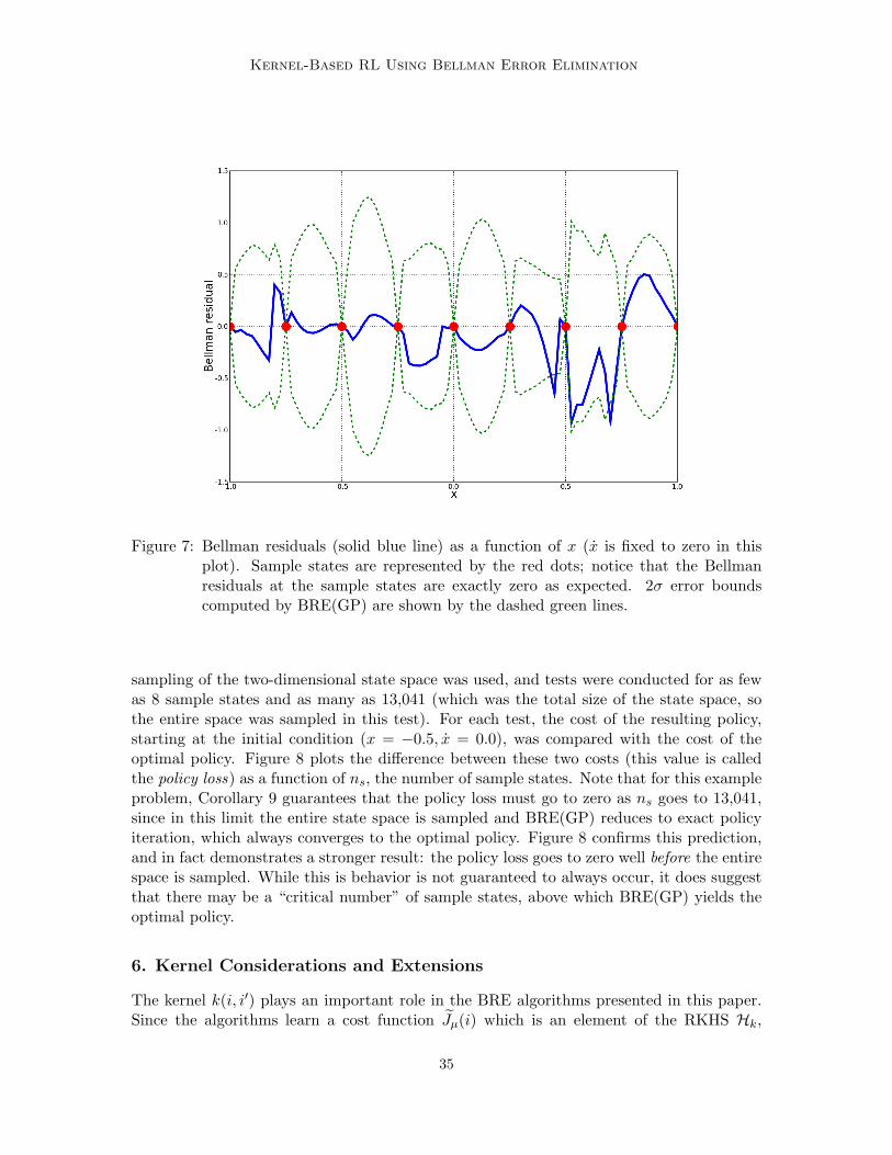
Kernel-Based RL Using Bellman Error Elimination
Figure 7: Bellman residuals (solid blue line) as a function of x (x is fixed to zero in thisplot). Sample states are represented by the red dots; notice that the Bellmanresiduals at the sample states are exactly zero as expected. 2σ error boundscomputed by BRE(GP) are shown by the dashed green lines.
sampling of the two-dimensional state space was used, and tests were conducted for as fewas 8 sample states and as many as 13,041 (which was the total size of the state space, sothe entire space was sampled in this test). For each test, the cost of the resulting policy,starting at the initial condition (x = −0.5, x = 0.0), was compared with the cost of theoptimal policy. Figure 8 plots the difference between these two costs (this value is calledthe policy loss) as a function of ns, the number of sample states. Note that for this exampleproblem, Corollary 9 guarantees that the policy loss must go to zero as ns goes to 13,041,since in this limit the entire state space is sampled and BRE(GP) reduces to exact policyiteration, which always converges to the optimal policy. Figure 8 confirms this prediction,and in fact demonstrates a stronger result: the policy loss goes to zero well before the entirespace is sampled. While this is behavior is not guaranteed to always occur, it does suggestthat there may be a “critical number” of sample states, above which BRE(GP) yields theoptimal policy.
6. Kernel Considerations and Extensions
The kernel k(i, i′) plays an important role in the BRE algorithms presented in this paper.Since the algorithms learn a cost function Jµ(i) which is an element of the RKHS Hk,
35
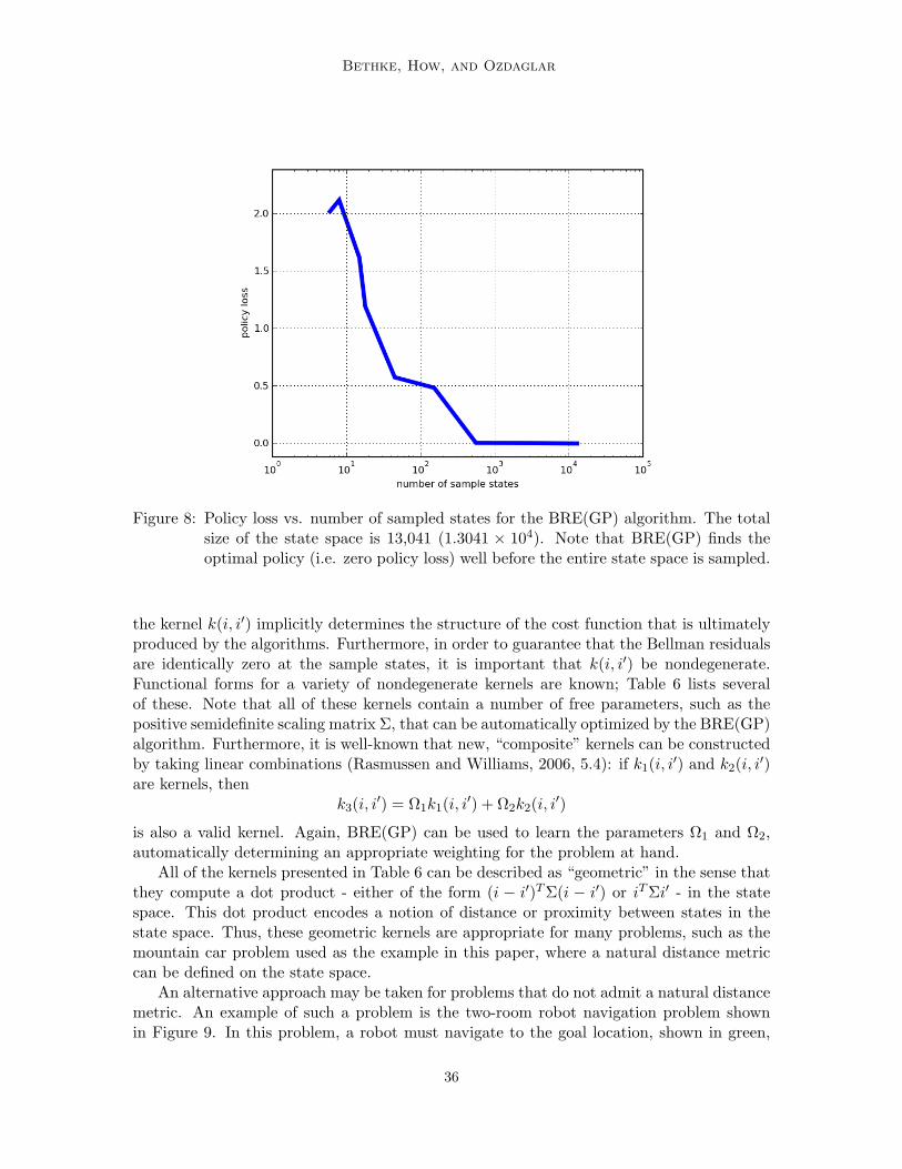
Bethke, How, and Ozdaglar
Figure 8: Policy loss vs. number of sampled states for the BRE(GP) algorithm. The totalsize of the state space is 13,041 (1.3041 × 10⁴). Note that BRE(GP) finds theoptimal policy (i.e. zero policy loss) well before the entire state space is sampled.
the kernel k(i, i′) implicitly determines the structure of the cost function that is ultimatelyproduced by the algorithms. Furthermore, in order to guarantee that the Bellman residualsare identically zero at the sample states, it is important that k(i, i′) be nondegenerate.Functional forms for a variety of nondegenerate kernels are known; Table 6 lists severalof these. Note that all of these kernels contain a number of free parameters, such as thepositive semidefinite scaling matrix Σ, that can be automatically optimized by the BRE(GP)algorithm. Furthermore, it is well-known that new, “composite” kernels can be constructedby taking linear combinations (Rasmussen and Williams, 2006, 5.4): if k1(i, i′) and k2(i, i′)are kernels, then
k3(i, i′) = Ω1k1(i, i′) + Ω2k2(i, i′)
is also a valid kernel. Again, BRE(GP) can be used to learn the parameters Ω1 and Ω2,automatically determining an appropriate weighting for the problem at hand.
All of the kernels presented in Table 6 can be described as “geometric” in the sense thatthey compute a dot product - either of the form (i − i′)T Σ(i − i′) or iT Σi′ - in the statespace. This dot product encodes a notion of distance or proximity between states in thestate space. Thus, these geometric kernels are appropriate for many problems, such as themountain car problem used as the example in this paper, where a natural distance metriccan be defined on the state space.
An alternative approach may be taken for problems that do not admit a natural distancemetric. An example of such a problem is the two-room robot navigation problem shownin Figure 9. In this problem, a robot must navigate to the goal location, shown in green,
36
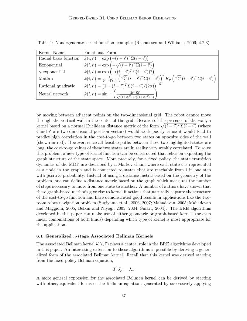
Kernel-Based RL Using Bellman Error Elimination
Table 1: Nondegenerate kernel function examples (Rasmussen and Williams, 2006, 4.2.3)
Kernel Name Functional FormRadial basis function k(i, i′) = exp
(−(i− i′)T Σ(i− i′)
)Exponential k(i, i′) = exp
(−√
(i− i′)T Σ(i− i′))
γ-exponential k(i, i′) = exp(−((i− i′)T Σ(i− i′))γ
)Matern k(i, i′) = 1
2ν−1Γ(ν)
(√2νl (i− i′)T Σ(i− i′)
)νKν
(√2νl (i− i′)T Σ(i− i′)
)Rational quadratic k(i, i′) =
(1 + (i− i′)T Σ(i− i′)/(2α)
)−α
Neural network k(i, i′) = sin−1
(2iT Σi′√
(1+2iT Σi′)(1+2i′T Σi)
)
by moving between adjacent points on the two-dimensional grid. The robot cannot movethrough the vertical wall in the center of the grid. Because of the presence of the wall, akernel based on a normal Euclidean distance metric of the form
√(i− i′)T Σ(i− i′) (where
i and i′ are two-dimensional position vectors) would work poorly, since it would tend topredict high correlation in the cost-to-go between two states on opposite sides of the wall(shown in red). However, since all feasible paths between these two highlighted states arelong, the cost-to-go values of these two states are in reality very weakly correlated. To solvethis problem, a new type of kernel function can be constructed that relies on exploiting thegraph structure of the state space. More precisely, for a fixed policy, the state transitiondynamics of the MDP are described by a Markov chain, where each state i is representedas a node in the graph and is connected to states that are reachable from i in one stepwith positive probability. Instead of using a distance metric based on the geometry of theproblem, one can define a distance metric based on the graph which measures the numberof steps necessary to move from one state to another. A number of authors have shown thatthese graph-based methods give rise to kernel functions that naturally capture the structureof the cost-to-go function and have demonstrated good results in applications like the two-room robot navigation problem (Sugiyama et al., 2006, 2007; Mahadevan, 2005; Mahadevanand Maggioni, 2005; Belkin and Niyogi, 2005, 2004; Smart, 2004). The BRE algorithmsdeveloped in this paper can make use of either geometric or graph-based kernels (or evenlinear combinations of both kinds) depending which type of kernel is most appropriate forthe application.
6.1 Generalized n-stage Associated Bellman Kernels
The associated Bellman kernel K(i, i′) plays a central role in the BRE algorithms developedin this paper. An interesting extension to these algorithms is possible by deriving a gener-alized form of the associated Bellman kernel. Recall that this kernel was derived startingfrom the fixed policy Bellman equation,
TµJµ = Jµ.
A more general expression for the associated Bellman kernel can be derived by startingwith other, equivalent forms of the Bellman equation, generated by successively applying
37
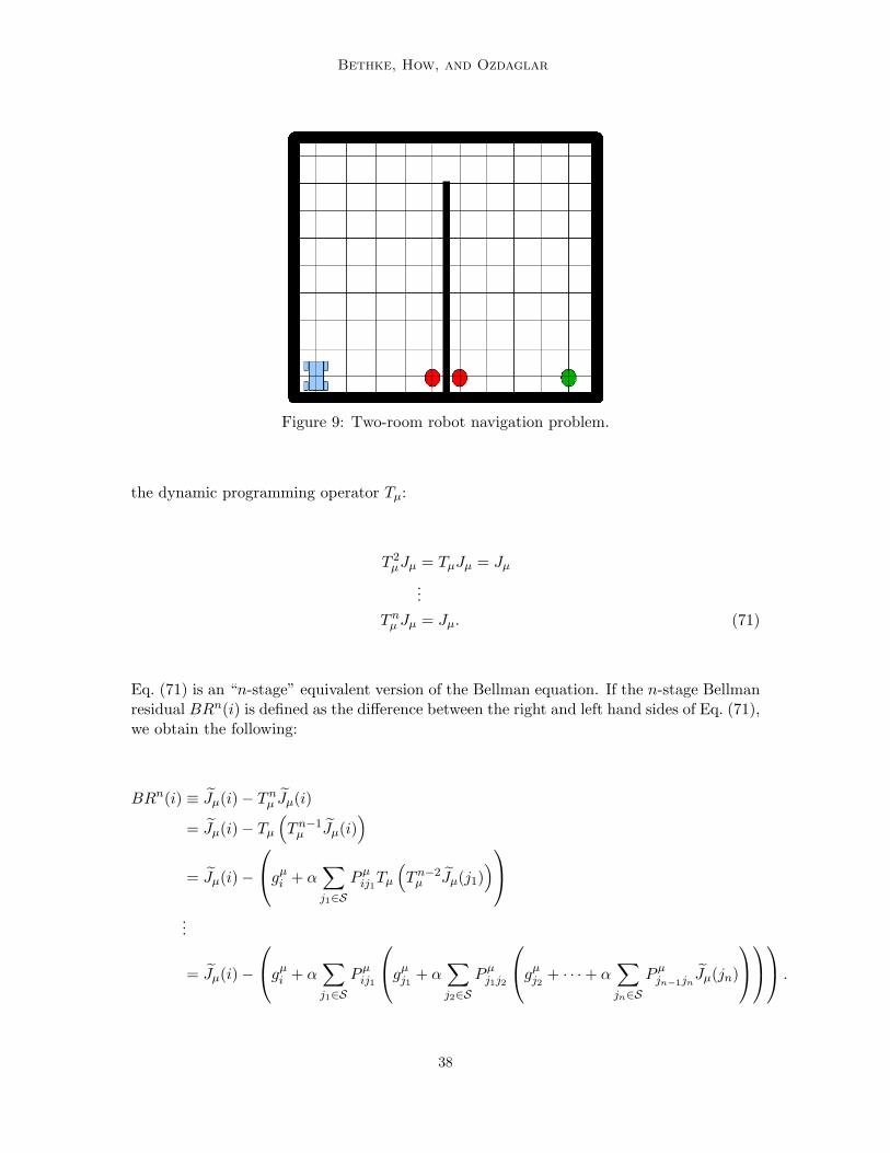
Bethke, How, and Ozdaglar
Figure 9: Two-room robot navigation problem.
the dynamic programming operator Tµ:
T 2µJµ = TµJµ = Jµ
...Tn
µ Jµ = Jµ. (71)
Eq. (71) is an “n-stage” equivalent version of the Bellman equation. If the n-stage Bellmanresidual BRn(i) is defined as the difference between the right and left hand sides of Eq. (71),we obtain the following:
BRn(i) ≡ Jµ(i)− Tnµ Jµ(i)
= Jµ(i)− Tµ
(Tn−1
µ Jµ(i))
= Jµ(i)−
gµi + α
∑j1∈S
Pµij1
Tµ
(Tn−2
µ Jµ(j1))
...
= Jµ(i)−
gµi + α
∑j1∈S
Pµij1
gµj1
+ α∑j2∈S
Pµj1j2
gµj2
+ · · ·+ α∑jn∈S
Pµjn−1jn
Jµ(jn)
.
38
Kernel-Based RL Using Bellman Error Elimination
Substituting the standard functional form Jµ(i) = 〈Θ,Φ(i)〉 into the expression for BRn(i)and using linearity of the inner product gives
BRn(i) = 〈Θ,Φ(i)〉
−
gµi + α
∑j1∈S
Pµij1
gµj1
+ α∑j2∈S
Pµj1j2
gµj2
+ · · ·+ α∑jn∈S
Pµjn−1jn
〈Θ,Φ(jn)〉
= 〈Θ,
Φ(i)− αn∑
j1,...,jn∈S
(Pµ
ij1. . . Pµ
jn−1jn
)Φ(jn)
〉−
gµi + α
∑j1∈S
Pµij1
gµj1
+ α∑j2∈S
Pµj1j2
gµj2
+ · · ·+ α∑
jn−1∈SPµ
jn−2jn−1gµjn−1
.
Finally, a new n-stage feature vector Ψn(i) and n-stage cost gn,µi can be defined as
Ψn(i) ≡ Φ(i)− αn∑
j1,...,jn∈S
(Pµ
ij1. . . Pµ
jn−1jn
)Φ(jn)
and
gn,µi ≡ gµ
i + α∑j1∈S
Pµij1
gµj1
+ α∑j2∈S
Pµj1j2
gµj2
+ · · ·+ α∑
jn−1∈SPµ
jn−2jn−1gµjn−1
,
respectively. Using these expressions, the n-stage Bellman residual can be expressed as
BRn(i) = 〈Θ,Ψn(i)〉 − gn,µi .
Therefore, in direct analogy with the derivation of the earlier BRE algorithms, solving theregression problem
Wnµ (i) = 〈Θ,Ψn(i)〉 = gn,µ
i ∀i ∈ S (72)
using the n-stage associated Bellman kernel given by
Kn(i, i′) = 〈Ψn(i),Ψn(i′)〉
is equivalent to finding a cost-to-go function of the form Jµ(i) = 〈Θ,Φ(i)〉 satisfying
Tnµ (i)Jµ(i) = Jµ(i) ∀i ∈ S.
Again, any kernel-based regression method can be used to solve the regression problemspecified by Eq. (72), resulting in a general class of n-stage Bellman residual eliminationalgorithms. It is possible to prove that these n-stage BRE algorithms possess all of the desir-able theoretical properties we have shown in this paper for single stage BRE. In particular,if the kernel k(i, i′) is nondegenerate, then the n-stage associated Bellman kernel Kn(i, i′) isnondegenerate, the n-stage Bellman residuals BRn(i) are identically zero at every samplestate, and the algorithms reduce to exact policy iteration in the limit of sampling the entirestate space.
39
Bethke, How, and Ozdaglar
The advantage obtained by working with the n-stage Bellman equation is that thealgorithm is forced to consider and adjust the relative values of more states in the statespace, resulting in a more accurate cost-to-go solution. Indeed, in the n-stage problem,the algorithm must consider the values of not only every state reachable in 1 step fromeach sample state i ∈ S, but every state reachable in n steps. This increased solutionaccuracy comes at a higher computational cost. If the average braching factor of the MDP(that is, the average number of edges per node in the state transition Markov chain) is m,then computing the n-stage associated Bellman kernel Kn(i, i′) involves O(mn) operations.For some problems, however, the branching factor may be small enough to allow practicalcomputation of Kn(i, i′) for n > 1. (In particular, n-stage BRE is especially appropriatefor deterministic problems, where the branching factor is 1 for every state). In these cases,n-stage BRE is practical to carry out and may increase the performance of the resultingpolicy. Future work will examine the performance of these n-stage BRE algorithms appliedto benchmark reinforcement learning problems.
7. Conclusion
This paper has demonstrated how kernel-based techniques can be used to design a new classof reinforcement learning algorithms that carry out Bellman residual elimination (BRE).These BRE algorithms learn the structure of the cost-to-go function by forcing the Bellmanresiduals to zero at a chosen set of representative sample states. Essentially, our approachreduces the dimensionality of the fixed-policy Bellman equation to a much smaller linearsystem that is practical to solve, and uses the solution to the smaller system in orderto infer the cost everywhere in the state space. The BRE algorithms have the desirabletheoretical property of reducing to exact policy iteration when the entire state space issampled, since in that case the algorithms effectively compute the solution to the full fixed-policy Bellman equation. Furthermore, by exploiting knowledge of the underlying MDPmodel, the algorithms avoid the need to carry out trajectory simulations and thus do notsuffer from simulation noise effects.
Application of our BRE algorithms to a classic reinforcement learning problem indicatesthat they yield nearly optimal policies while requiring relatively few sample states (andtherefore, can be computed efficiently). The kernel parameter learning mechanism employedby BRE(GP) was demonstrated to be effective at finding appropriate values of the kernelparameters. This is an important feature of the BRE(GP) algorithm, especially in higher-dimensional and more complex problems where suitable values of the kernel parametersmay not be known a priori. Furthermore, the error bounds computed by BRE(GP) can beused not only for predicting the quality of the computed cost function, but also for activelychoosing which regions of the state space to sample (i.e. by selecting more sample states inregions where the error is large).
Based on both the theoretical results (in particular, that our BRE algorithms are guar-anteed to yield the optimal policy when all states are sampled) and experimental validationpresented in this paper, we believe that our Bellman residual elimination algorithms offera useful approach for efficiently solving large-scale reinforcement learning problems.
40
Kernel-Based RL Using Bellman Error Elimination
Acknowledgments
Research supported by the Hertz Foundation, the American Society for Engineering Edu-cation, and the Boeing Company.
Appendix A. Proofs
Lemma 1 Assume the vectors Φ(i) | i ∈ S are linearly independent. Then the vectorsΨ(i) | i ∈ S, where Ψ(i) = Φ(i)− α
∑j∈S Pµ
ijΦ(j), are also linearly independent.Proof Consider the real vector space V spanned by the vectors Φ(i) | i ∈ S. It is clearthat Ψ(i) is a linear combination of vectors in V, so a linear operator B that maps Φ(i) toΨ(i) can be defined:
Ψ(i) = BΦ(i).
SinceΨ(i) = Φ(i)− α
∑j∈S
PµijΦ(j),
the matrix of B is(I − αPµ),
where I is the identity matrix and Pµ is the probability transition matrix for the policyµ. Since Pµ is a stochastic matrix, its largest eigenvalue is 1 and all other eigenvalueshave absolute value less than 1; hence all eigenvalues of αPµ have absolute value less thanor equal to α < 1. Since all eigenvalues of I are equal to 1, (I − αPµ) is full rank anddim(ker(B)) = 0. Therefore,
dim(Ψ(i) | i ∈ S) = dim(Φ(i) | i ∈ S) = ns
so the vectors Ψ(i) | i ∈ S are linearly independent.
Theorem 2 Assume that the kernel k(i, i′) = 〈Φ(i),Φ(i′)〉 is nondegenerate. Then the asso-ciated Bellman kernel defined by K(i, i′) = 〈Ψ(i),Ψ(i′)〉, where Ψ(i) = Φ(i)−α
∑j∈S Pµ
ijΦ(j),is also nondegenerate.Proof Since k(i, i′) is nondegenerate, the vectors Φ(i) | i ∈ S are linearly independent.Therefore, Lemma 1 applies, and the vectors Ψ(i) | i ∈ S are linearly independent, im-mediately implying that K(i, i′) is nondegenerate.
Theorem 3 Assume that the kernel k(i, i′) = 〈Φ(i),Φ(i′)〉 is nondegenerate. Then thecost-to-go function Jµ(i) produced by Algorithm 2 satisfies
Jµ(i) = gµi + α
∑j∈S
Pµij Jµ(j) ∀i ∈ S.
That is, the Bellman residuals BR(i) are identically zero at every state i ∈ S.Proof Since k(i, i′) is nondegenerate, Theorem 2 applies and K(i, i′) is also nondegenerate.Therefore, the Gram matrix K of K(i, i′) is positive definite and invertible. It follows that,
41
Bethke, How, and Ozdaglar
in Line 8 of Algorithm 2, there is a unique solution for λ. Having found a feasible solutionλ for the dual problem given by [Eq. (49)], Slater’s condition is satisfied and strong dualityholds. Therefore, the primal problem [Eq. (45)] is feasible, and its optimal solution is givenby Eq. (47). Feasibility of this solution implies
BR(i) = −gµi + 〈Θ,Ψ(i)〉 = 0 ∀i ∈ S
as claimed.
Corollary 4 Assume that the kernel k(i, i′) = 〈Φ(i),Φ(i′)〉 is nondegenerate, and thatS = S. Then the cost-to-go function Jµ(i) produced by Algorithm 2 satisfies
Jµ(i) = Jµ(i) ∀i ∈ S.
That is, the cost function Jµ(i) is exact.Proof Applying Theorem 3 with S = S, we have
BR(i) = 0 ∀i ∈ S.
Using the definition of the Bellman residual,
BR(i) ≡ Jµ(i)− TµJµ(i),
immediately implies thatJµ(i) = TµJµ(i) ∀i ∈ S.
Therefore, Jµ(i) satisfies the fixed-policy Bellman equation, so
Jµ(i) = Jµ(i) ∀i ∈ S
as claimed.
Corollary 5 Assume that the kernel k(i, i′) = 〈Φ(i),Φ(i′)〉 is nondegenerate, and thatS = S. Then BRE(SV) (given in Algorithm 3) is equivalent to exact policy iteration.Proof By Corollary 4, the cost function Jµ(i) produced by BRE(SV) is equal to the exactcost Jµ(i), at every state i ∈ S. Since the policy improvement step (Line 9) is also exact,BRE(SV) carries out exact policy iteration by definition, and converges in a finite numberof steps to the optimal policy.
Theorem 6 Assume that the kernel k(i, i′) = 〈Φ(i),Φ(i′)〉 is nondegenerate. Then thereexists a linear, invertible mapping A from Hk, the RKHS of k, to HK, the RKHS of theassociated Bellman kernel K:
A : Hk → HKAJµ(·) = Wµ(·).
42
Kernel-Based RL Using Bellman Error Elimination
Furthermore, if an element Jµ(·) ∈ Hk is given by
Jµ(·) = 〈Θ,Φ(·)〉,
then the corresponding element Wµ(·) ∈ HK is given by
Wµ(·) = 〈Θ,Ψ(·)〉, (73)
and vice versa:
Jµ(·) = 〈Θ,Φ(·)〉m
Wµ(·) = 〈Θ,Ψ(·)〉.
Proof Recall from the proof of Lemma 1 that the relation between Φ(i) and Ψ(i) [Eq. (53)]is defined by the invertible linear operator B:
Ψ(i) = BΦ(i)
Using the definition of B and linearity of the inner product 〈·, ·〉, Eq. (73) can be rewrittenas
Wµ(·) = 〈Θ, BΦ(·)〉= B〈Θ,Φ(·)〉= BJµ(·),
which establishes the invertible linear mapping between Hk and HK, as claimed. Therefore,the linear mapping A in the statement of the theorem exists and is equal to the linearmapping B from Lemma 1:
A = B.
Comparing Eqs. (57) and (62), notice that we can convert between a cost function Jµ(·)and its corresponding function Wµ(·) by replacing Φ(·) with Ψ(·) in the inner product:
Jµ(·) = 〈Θ,Φ(·)〉m
Wµ(·) = 〈Θ,Ψ(·)〉
Theorem 7 Assume that the kernel k(i, i′; Ω) = 〈Φ(i; Ω),Φ(i′; Ω)〉 is nondegenerate. Thenthe cost-to-go functions Jµ(i) computed by BRE(GP) (on line 17) satisfy
Jµ(i) = gµi + α
∑j∈S
Pµij Jµ(j) ∀i ∈ S.
43
Bethke, How, and Ozdaglar
That is, the Bellman residuals BR(i) are identically zero at every state i ∈ S.Proof Note that line 13 of the BRE(GP) algorithm computes the weights λ as
λ = K(Ω)−1gµ.
Aside from the purely notational difference emphasizing the dependence of the Gram ma-trix K(Ω) on the kernel parameters Ω, the weights λ and the cost function Jµ(i) computedby BRE(GP) are identical to those computed by BRE(SV). Therefore, Theorem 3 appliesdirectly, and the Bellman residuals are identically zero at every state i ∈ S.
Corollary 8 Assume that the kernel k(i, i′; Ω) = 〈Φ(i; Ω),Φ(i′; Ω)〉 is nondegenerate, andthat S = S. Then the cost-to-go function Jµ(i) produced by BRE(GP) satisfies
Jµ(i) = Jµ(i) ∀i ∈ S.
That is, the cost function Jµ(i) is exact.Proof Applying Theorem 7 with S = S, we have
BR(i) = 0 ∀i ∈ S.
Using the definition of the Bellman residual,
BR(i) ≡ Jµ(i)− TµJµ(i),
immediately implies thatJµ(i) = TµJµ(i) ∀i ∈ S.
Therefore, Jµ(i) satisfies the fixed-policy Bellman equation, so
Jµ(i) = Jµ(i) ∀i ∈ S
as claimed.
Corollary 9 Assume that the kernel k(i, i′; Ω) = 〈Φ(i; Ω),Φ(i′; Ω)〉 is nondegenerate, andthat S = S. Then BRE(GP) is equivalent to exact policy iteration.Proof By Corollary 4, we have that the cost produced by BRE(GP), Jµ(i) is equal tothe exact cost Jµ(i), at every state i ∈ S. Since the policy improvement step (Line 19) isalso exact, the algorithm carries out exact policy iteration by definition, and converges ina finite number of steps to the optimal policy.
References
A. Antos, C. Szepesvari, and R. Munos. Learning near-optimal policies with bellman-residual minimization based fitted policy iteration and a single sample path. MachineLearning, 71(1):89–129, 2008.
44
Kernel-Based RL Using Bellman Error Elimination
N. Aronszajn. Theory of reproducing kernels. Transactions of the American MathematicalSociety, 68:337–404, 1950.
L. C. Baird. Residual algorithms: Reinforcement learning with function approximation. InICML, pages 30–37, 1995.
M. Belkin and P. Niyogi. Towards a theoretical foundation for laplacian-based manifoldmethods. In Peter Auer and Ron Meir, editors, COLT, volume 3559 of Lecture Notes inComputer Science, pages 486–500. Springer, 2005. ISBN 3-540-26556-2.
M. Belkin and P. Niyogi. Semi-supervised learning on riemannian manifolds. MachineLearning, 56(1-3):209–239, 2004.
C. Berg, J. Christensen, and P. Ressel. Harmonic Analysis on Semigroups. Springer-Verlag,New York, 1984.
D. Bertsekas. Dynamic Programming and Optimal Control. Athena Scientific, Belmont,MA, 2007.
D. Bertsekas and S. Ioffe. Temporal Differences-Based Policy Iteration and Applications inNeuro-Dynamic Programming. http://web.mit.edu/people/dimitrib/Tempdif.pdf, 1996.
D. Bertsekas and J. Tsitsiklis. Neuro-Dynamic Programming. Athena Scientific, Belmont,MA, 1996.
C. M. Bishop. Neural networks for pattern recognition. Oxford University Press, 1995.
C. J. C. Burges. A tutorial on support vector machines for pattern recognition. In KnowledgeDiscovery and Data Mining, number 2, 1998.
J. Candela and C. Rasmussen. A unifying view of sparse approximate gaussian processregression. Journal of Machine Learning Research, 6:1939–1959, 2005.
C. Chang and C. Lin. LIBSVM: a library for support vector machines, 2001. Softwareavailable at http://www.csie.ntu.edu.tw/ cjlin/libsvm.
N. Christianini and J. Shawe-Taylor. Support Vector Machines and Other kernel-basedLearning Methods. Cambridge University Press, 2000.
DP de Farias and B. Van Roy. The Linear Programming Approach to Approximate DynamicProgramming. Operations Research, 51(6):850–865, 2003.
M. Deisenroth, J. Peters, and C. Rasmussen. Approximate dynamic programming withgaussian processes. In Proceedings of the American Control Conference, 2008.
T. Dietterich and X. Wang. Batch value function approximation via support vectors. InThomas G. Dietterich, Suzanna Becker, and Zoubin Ghahramani, editors, NIPS, pages1491–1498. MIT Press, 2001.
Y. Engel. Algorithms and Representations for Reinforcement Learning. PhD thesis, HebrewUniversity, 2005.
45
Bethke, How, and Ozdaglar
Y. Engel, S. Mannor, and Ron Meir. Bayes meets bellman: The gaussian process approachto temporal difference learning. In Tom Fawcett and Nina Mishra, editors, ICML, pages154–161. AAAI Press, 2003. ISBN 1-57735-189-4.
Y. Engel, S. Mannor, and R. Meir. Reinforcement learning with gaussian processes. InLuc De Raedt and Stefan Wrobel, editors, ICML, volume 119 of ACM InternationalConference Proceeding Series, pages 201–208. ACM, 2005. ISBN 1-59593-180-5.
F. Girosi. An equivalence between sparse approximation and support vector machines.Neural Computation, 10(6):1455–1480, 1998.
S. Haykin. Neural Networks: A Comprehensive Foundation. Macmillan, New York, 1994.
K. Hornik, M. Stinchcombe, and H. White. Multilayer feedforward networks are universalapproximators. Neural Networks, 2(5):359–366, 1989.
S. Keerthi, S. Shevade, C. Bhattacharyya, and K. Murthy. Improvements to Platt’s SMOalgorithm for SVM classifier design. http://citeseer.ist.psu.edu/244558.html, 1999.
M. Lagoudakis and R. Parr. Least-squares policy iteration. Journal of Machine LearningResearch, 4:1107–1149, 2003. ISSN 1533-7928.
M. Maggioni and S. Mahadevan. Fast direct policy evaluation using multiscale analysis ofmarkov diffusion processes. In William W. Cohen and Andrew Moore, editors, ICML,volume 148 of ACM International Conference Proceeding Series, pages 601–608. ACM,2006. ISBN 1-59593-383-2.
S. Mahadevan. Proto-value functions: Developmental reinforcement learning. In Interna-tional Conference on Machine Learning, 2005.
S. Mahadevan and M. Maggioni. Value function approximation with diffusion wavelets andlaplacian eigenfunctions. In NIPS, 2005.
R. Munos and C. Szepesvari. Finite-time bounds for fitted value iteration. Journal ofMachine Learning Research, 1:815–857, 2008.
D. Ormoneit and S. Sen. Kernel-Based Reinforcement Learning. Machine Learning, 49(2):161–178, 2002.
J. Platt. Using sparseness and analytic QP to speed training of support vector machines.In Advances in Neural Information Processing Systems, pages 557–563, 1999.
M. Puterman. Markov Decision Processes: Discrete Stochastic Dynamic Programming.Wiley, 1994.
C. Rasmussen and M. Kuss. Gaussian processes in reinforcement learning. Advances inNeural Information Processing Systems, 16:751–759, 2004.
C. Rasmussen and C. Williams. Gaussian Processes for Machine Learning. MIT Press,Cambridge, MA, 2006.
46
Kernel-Based RL Using Bellman Error Elimination
J. Reisinger, P. Stone, and R. Miikkulainen. Online kernel selection for bayesian reinforce-ment learning. In Proceedings of the 25th International Conference on Machine Learning,2008.
S. Saitoh. Theory of Reproducing Kernels and its Applications. Longman Scientific andTechnical, Harlow, England, 1988.
B. Scholkopf. Support Vector Learning. Available fromhttp://www.kyb.tuebingen.mpg.de/-bs, 1997.
B. Scholkopf and A. Smola. Learning with Kernels: Support Vector Machines, Regulariza-tion, Optimization, and Beyond. MIT Press, Cambridge, MA, 2002.
P. Schweitzer and A. Seidman. Generalized polynomial approximation in Markovian decisionprocesses. Journal of mathematical analysis and applications, 110:568–582, 1985.
A. Barto W. Powell J. Si and D. Wunsch. Learning and Approximate Dynamic Program-ming. IEEE Press, NY, 2004. URL http://citeseer.ist.psu.edu/651143.html.
W. Smart. Explicit manifold representations for value-function approximation in reinforce-ment learning. In AMAI, 2004.
A. Smola and B. Scholkopf. A Tutorial on Support Vector Regression. Statistics andComputing, 14:199–222, 2004.
M. Sugiyama, H. Hachiya, C. Towell, and S. Vijayakumar. Geodesic gaussian kernels forvalue function approximation. In Workshop on Information-Based Induction Sciences,2006.
M. Sugiyama, H. Hachiya, C. Towell, and S. Vijayakumar. Value function approximationon non-linear manifolds for robot motor control. In Proc. of the IEEE InternationalConference on Robotics and Automation, 2007.
R. Sutton and A. Barto. Reinforcement learning: An introduction. MIT Press, 1998.
G. Tesauro. Practical issues in temporal difference learning. Machine Learning, 8:257–277,1992.
G. Tesauro. Temporal difference learning and TD-Gammon. Commun. ACM, 38(3):58–68,1995. ISSN 0001-0782. doi: http://doi.acm.org/10.1145/203330.203343.
J. Tobias and P. Daniel. Least squares svm for least squares td learning. In Gerhard Brewka,Silvia Coradeschi, Anna Perini, and Paolo Traverso, editors, ECAI, pages 499–503. IOSPress, 2006. ISBN 1-58603-642-4.
M. A. Trick and S. E. Zin. Spline Approximations to Value Functions. MacroeconomicDynamics, 1:255?–277, January 1997.
M. Valenti. Approximate Dynamic Programming with Applications in Multi-Agent Systems.PhD thesis, Massachusetts Institute of Technology, 2007.
47
Bethke, How, and Ozdaglar
G. Wahba. Spline Models for Observational Data. In Vol. 59 of CBMS-NSF RegionalConference Series in Applied Mathematics, SIAM, Philidelphia, 1990.
48


![Antony and Cleopatra [James F. Bellman, Kathryn Bellman]](https://img.pdfslide.us/doc/110x75/55cf9761550346d03391502a/antony-and-cleopatra-james-f-bellman-kathryn-bellman.jpg)