Contents Outline The Kenward–Roger modification of the F–statistic Parametric bootstrap Small simulation study: A random regression problem Final remarks

Kenward-Roger modification of the F-statistic forsome linear mixed models fitted with lmer

Ulrich Halekoh 1 Søren Højsgaard 2

1Department of Molecular Biology and GeneticsAarhus University, Denmarkulrich.halekoh@agrsci.dk

2Department of Mathematical SciencesAalborg University, Denmark

sorenh@math.aau.dk

9. november 2011

1 / 23

Contents Outline The Kenward–Roger modification of the F–statistic Parametric bootstrap Small simulation study: A random regression problem Final remarks

1 Outline

Motivation: Sugar beets - A split–plot experiment

Motivation: A random regression problem

Our goal

2 The Kenward–Roger modification of the F –statistic

3 Parametric bootstrap

4 Small simulation study: A random regression problem

5 Final remarks

2 / 23

Contents Outline The Kenward–Roger modification of the F–statistic Parametric bootstrap Small simulation study: A random regression problem Final remarks

Motivation: Sugar beets - A split–plot experiment

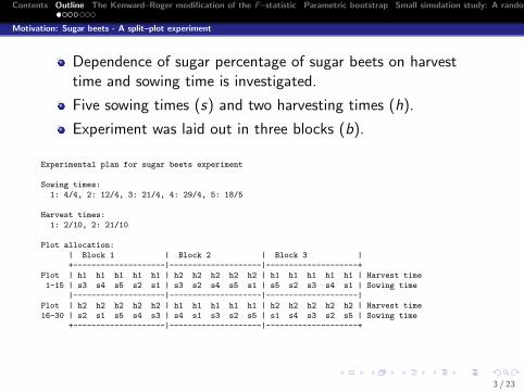
Dependence of sugar percentage of sugar beets on harvesttime and sowing time is investigated.

Five sowing times (s) and two harvesting times (h).

Experiment was laid out in three blocks (b).

Experimental plan for sugar beets experiment

Sowing times:

1: 4/4, 2: 12/4, 3: 21/4, 4: 29/4, 5: 18/5

Harvest times:

1: 2/10, 2: 21/10

Plot allocation:

| Block 1 | Block 2 | Block 3 |

+--------------------|--------------------|--------------------+

Plot | h1 h1 h1 h1 h1 | h2 h2 h2 h2 h2 | h1 h1 h1 h1 h1 | Harvest time

1-15 | s3 s4 s5 s2 s1 | s3 s2 s4 s5 s1 | s5 s2 s3 s4 s1 | Sowing time

|--------------------|--------------------|--------------------|

Plot | h2 h2 h2 h2 h2 | h1 h1 h1 h1 h1 | h2 h2 h2 h2 h2 | Harvest time

16-30 | s2 s1 s5 s4 s3 | s4 s1 s3 s2 s5 | s1 s4 s3 s2 s5 | Sowing time

+--------------------|--------------------|--------------------+

3 / 23

Contents Outline The Kenward–Roger modification of the F–statistic Parametric bootstrap Small simulation study: A random regression problem Final remarks

Motivation: Sugar beets - A split–plot experiment

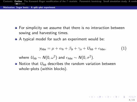
For simplicity we assume that there is no interaction betweensowing and harvesting times.

A typical model for such an experiment would be:

yhbs = µ+ αh + βb + γs + Uhb + εhbs , (1)

where Uhb ∼ N(0, ω2) and εhbs ∼ N(0, σ2).

Notice that Uhb describes the random variation betweenwhole–plots (within blocks).

4 / 23

Contents Outline The Kenward–Roger modification of the F–statistic Parametric bootstrap Small simulation study: A random regression problem Final remarks

Motivation: Sugar beets - A split–plot experiment

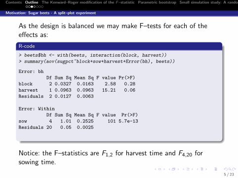
As the design is balanced we may make F–tests for each of theeffects as:

R-code

> beets$bh <- with(beets, interaction(block, harvest))

> summary(aov(sugpct~block+sow+harvest+Error(bh), beets))

Error: bh

Df Sum Sq Mean Sq F value Pr(>F)

block 2 0.0327 0.0163 2.58 0.28

harvest 1 0.0963 0.0963 15.21 0.06

Residuals 2 0.0127 0.0063

Error: Within

Df Sum Sq Mean Sq F value Pr(>F)

sow 4 1.01 0.2525 101 5.7e-13

Residuals 20 0.05 0.0025

Notice: the F–statistics are F1,2 for harvest time and F4,20 forsowing time.

5 / 23

Contents Outline The Kenward–Roger modification of the F–statistic Parametric bootstrap Small simulation study: A random regression problem Final remarks

Motivation: Sugar beets - A split–plot experiment

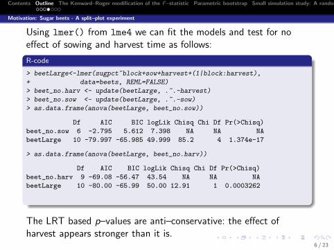
Using lmer() from lme4 we can fit the models and test for noeffect of sowing and harvest time as follows:

R-code

> beetLarge<-lmer(sugpct~block+sow+harvest+(1|block:harvest),

+ data=beets, REML=FALSE)

> beet_no.harv <- update(beetLarge, .~.-harvest)

> beet_no.sow <- update(beetLarge, .~.-sow)

> as.data.frame(anova(beetLarge, beet_no.sow))

Df AIC BIC logLik Chisq Chi Df Pr(>Chisq)

beet_no.sow 6 -2.795 5.612 7.398 NA NA NA

beetLarge 10 -79.997 -65.985 49.999 85.2 4 1.374e-17

> as.data.frame(anova(beetLarge, beet_no.harv))

Df AIC BIC logLik Chisq Chi Df Pr(>Chisq)

beet_no.harv 9 -69.08 -56.47 43.54 NA NA NA

beetLarge 10 -80.00 -65.99 50.00 12.91 1 0.0003262

The LRT based p–values are anti–conservative: the effect ofharvest appears stronger than it is.

6 / 23

Contents Outline The Kenward–Roger modification of the F–statistic Parametric bootstrap Small simulation study: A random regression problem Final remarks

Motivation: A random regression problem

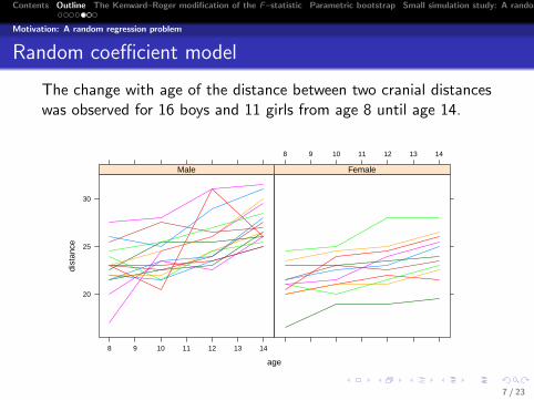
Random coefficient model

The change with age of the distance between two cranial distanceswas observed for 16 boys and 11 girls from age 8 until age 14.

age

dist

ance

20

25

30

8 9 10 11 12 13 14

Male

8 9 10 11 12 13 14

Female

7 / 23

Contents Outline The Kenward–Roger modification of the F–statistic Parametric bootstrap Small simulation study: A random regression problem Final remarks

Motivation: A random regression problem

Random coefficient model

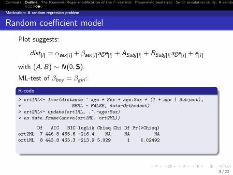
Plot suggests:

dist[i ] = αsex[i ] + βsex[i ]age[i ] + ASubj[i ] + BSubj[i ]age[i ] + e[i ]

with (A,B) ∼ N(0,S).

ML-test of βboy = βgirl :

R-code

> ort1ML<- lmer(distance ~ age + Sex + age:Sex + (1 + age | Subject),

+ REML = FALSE, data=Orthodont)

> ort2ML<- update(ort1ML, .~.-age:Sex)

> as.data.frame(anova(ort1ML, ort2ML))

Df AIC BIC logLik Chisq Chi Df Pr(>Chisq)

ort2ML 7 446.8 465.6 -216.4 NA NA NA

ort1ML 8 443.8 465.3 -213.9 5.029 1 0.02492

8 / 23

Contents Outline The Kenward–Roger modification of the F–statistic Parametric bootstrap Small simulation study: A random regression problem Final remarks

Our goal

Our goal...

Our goal is to extend the tests provided by lmer().

There are two issues here:

The choice of test statistic and

The reference distribution in which the test statistic isevaluated.

9 / 23

Contents Outline The Kenward–Roger modification of the F–statistic Parametric bootstrap Small simulation study: A random regression problem Final remarks

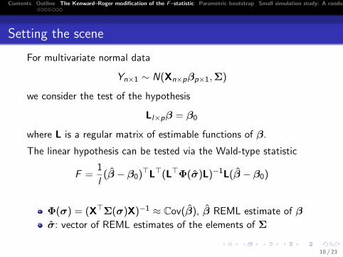
Setting the scene

For multivariate normal data

Yn×1 ∼ N(Xn×pβp×1,Σ)

we consider the test of the hypothesis

Ll×pβ = β0

where L is a regular matrix of estimable functions of β.

The linear hypothesis can be tested via the Wald-type statistic

F =1

l(β̂ − β0)>L>(L>Φ(σ̂)L)−1L(β̂ − β0)

Φ(σ) = (X>Σ(σ)X)−1 ≈ Cov(β̂), β̂ REML estimate of β

σ̂: vector of REML estimates of the elements of Σ

10 / 23

Contents Outline The Kenward–Roger modification of the F–statistic Parametric bootstrap Small simulation study: A random regression problem Final remarks

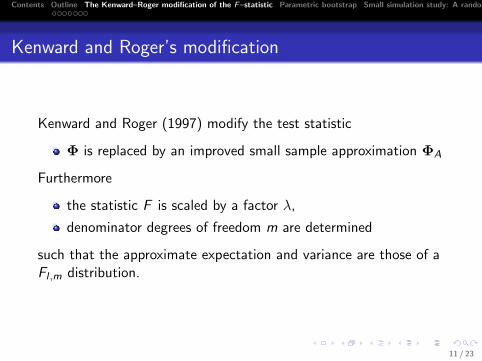
Kenward and Roger’s modification

Kenward and Roger (1997) modify the test statistic

Φ is replaced by an improved small sample approximation ΦA

Furthermore

the statistic F is scaled by a factor λ,

denominator degrees of freedom m are determined

such that the approximate expectation and variance are those of aFl ,m distribution.

11 / 23

Contents Outline The Kenward–Roger modification of the F–statistic Parametric bootstrap Small simulation study: A random regression problem Final remarks

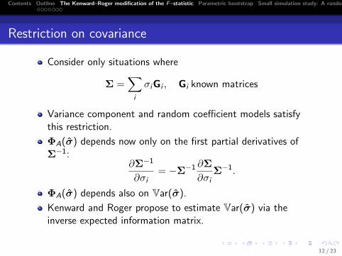
Restriction on covariance

Consider only situations where

Σ =∑i

σiGi , Gi known matrices

Variance component and random coefficient models satisfythis restriction.

ΦA(σ̂) depends now only on the first partial derivatives ofΣ−1:

∂Σ−1

∂σi= −Σ−1 ∂Σ

∂σiΣ−1.

ΦA(σ̂) depends also on Var(σ̂).

Kenward and Roger propose to estimate Var(σ̂) via theinverse expected information matrix.

12 / 23

Contents Outline The Kenward–Roger modification of the F–statistic Parametric bootstrap Small simulation study: A random regression problem Final remarks

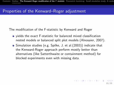
Properties of the Kenward–Roger adjustment

The modification of the F-statistic by Kenward and Roger

yields the exact F-statistic for balanced mixed classificationnested models or balanced split plot models (Alnosaier, 2007).

Simulation studies (e.g. Spilke, J. et al.(2003)) indicate thatthe Kenward-Roger approach perform mostly better thanalternatives (like Satterthwaite or containment method) forblocked experiments even with missing data.

13 / 23

Contents Outline The Kenward–Roger modification of the F–statistic Parametric bootstrap Small simulation study: A random regression problem Final remarks

R package lme4

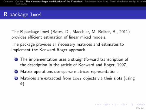
The R package lme4 (Bates, D., Maechler, M, Bolker, B., 2011)provides efficient estimation of linear mixed models.

The package provides all necessary matrices and estimates toimplement the Kenward-Roger approach.

1 The implementation uses a straightforward transcription ofthe description in the article of Kenward and Roger, 1997.

2 Matrix operations use sparse matrices representation.

3 Matrices are extracted from lmer objects via their slots (using@).

14 / 23

Contents Outline The Kenward–Roger modification of the F–statistic Parametric bootstrap Small simulation study: A random regression problem Final remarks

Kenward–Roger: split-plot (sugar-beets)

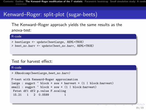
The Kenward–Roger approach yields the same results as theanova-test:

R-code

> beetLarge <- update(beetLarge, REML=TRUE)

> beet_no.harv <- update(beet_no.harv, REML=TRUE)

Test for harvest effect:

R-code

> KRmodcomp(beetLarge,beet_no.harv)

F-test with Kenward-Roger approximation

large : sugpct ~ block + sow + harvest + (1 | block:harvest)

small : sugpct ~ block + sow + (1 | block:harvest)

Fstat df1 df2 p.value F.scaling

15.21 1 2 0.0599 1

15 / 23

Contents Outline The Kenward–Roger modification of the F–statistic Parametric bootstrap Small simulation study: A random regression problem Final remarks

Kenward–Roger: random regression (cranial change)

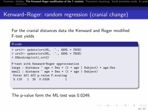
For the cranial distances data the Kenward and Roger modifiedF-test yields

R-code

> ort1<- update(ort1ML, .~., REML = TRUE)

> ort2<- update(ort2ML, .~., REML = TRUE)

> KRmodcomp(ort1,ort2)

F-test with Kenward-Roger approximation

large : distance ~ age + Sex + (1 + age | Subject) + age:Sex

small : distance ~ age + Sex + (1 + age | Subject)

Fstat df1 df2 p.value F.scaling

5.118 1 25 0.0326 1

The p-value form the ML-test was 0.0249.

16 / 23

Contents Outline The Kenward–Roger modification of the F–statistic Parametric bootstrap Small simulation study: A random regression problem Final remarks

Using parametric bootstrap

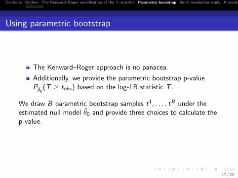
The Kenward–Roger approach is no panacea.

Additionally, we provide the parametric bootstrap p-valuePθ̂0

(T ≥ tobs) based on the log-LR statistic T .

We draw B parametric bootstrap samples t1, . . . , tB under theestimated null model θ̂0 and provide three choices to calculate thep-value.

17 / 23

Contents Outline The Kenward–Roger modification of the F–statistic Parametric bootstrap Small simulation study: A random regression problem Final remarks

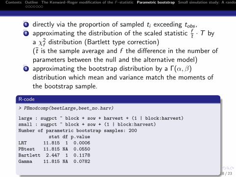
1 directly via the proportion of sampled ti exceeding tobs ,2 approximating the distribution of the scaled statistic f

t̄ · T bya χ2

f distribution (Bartlett type correction)(t̄ is the sample average and f the difference in the number ofparameters between the null and the alternative model)

3 approximating the bootstrap distribution by a Γ(α, β)distribution which mean and variance match the moments ofthe bootstrap sample.

R-code

> PBmodcomp(beetLarge,beet_no.harv)

large : sugpct ~ block + sow + harvest + (1 | block:harvest)

small : sugpct ~ block + sow + (1 | block:harvest)

Number of parametric bootstrap samples: 200

stat df p.value

LRT 11.815 1 0.0006

PBtest 11.815 NA 0.0550

Bartlett 2.447 1 0.1178

Gamma 11.815 NA 0.0782

18 / 23

Contents Outline The Kenward–Roger modification of the F–statistic Parametric bootstrap Small simulation study: A random regression problem Final remarks

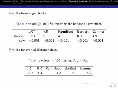
Results from sugar beets:

Tabel: p-values (× 100) for removing the harvest or sow effect.

LRT KR ParmBoot Bartlett Gamma

harvest 0.03 6 4.1 8.3 4.9sow <0.001 <0.001 <0.001 <0.001 <0.001

Results for cranial distance data:

Tabel: p-values (× 100) testing βboy = βgirl .

LRT KR ParmBoot Bartlett Gamma

2.5 3.3 4.2 4.0 4.2

19 / 23

Contents Outline The Kenward–Roger modification of the F–statistic Parametric bootstrap Small simulation study: A random regression problem Final remarks

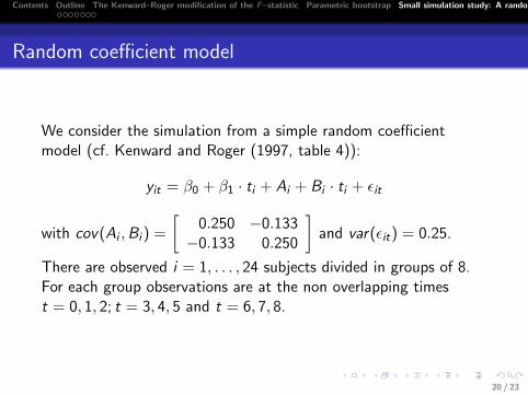
Random coefficient model

We consider the simulation from a simple random coefficientmodel (cf. Kenward and Roger (1997, table 4)):

yit = β0 + β1 · ti + Ai + Bi · ti + εit

with cov(Ai ,Bi ) =

[0.250 −0.133

−0.133 0.250

]and var(εit) = 0.25.

There are observed i = 1, . . . , 24 subjects divided in groups of 8.For each group observations are at the non overlapping timest = 0, 1, 2; t = 3, 4, 5 and t = 6, 7, 8.

20 / 23

Contents Outline The Kenward–Roger modification of the F–statistic Parametric bootstrap Small simulation study: A random regression problem Final remarks

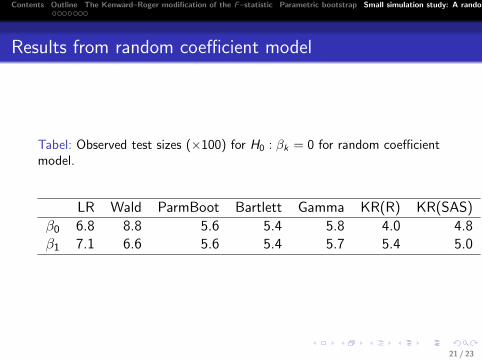
Results from random coefficient model

Tabel: Observed test sizes (×100) for H0 : βk = 0 for random coefficientmodel.

LR Wald ParmBoot Bartlett Gamma KR(R) KR(SAS)

β0 6.8 8.8 5.6 5.4 5.8 4.0 4.8β1 7.1 6.6 5.6 5.4 5.7 5.4 5.0

21 / 23

Contents Outline The Kenward–Roger modification of the F–statistic Parametric bootstrap Small simulation study: A random regression problem Final remarks

Summary

The functions KRmodcomp() and PBmodcomp() described hereare available in the pbkrtest package.

The Kenward–Roger approach requires fitting by REML; theparametric bootstrap approaches requires fitting by ML.

The required fitting scheme is set by the relevant functions, sothe user needs not worry about this.

Parametric bootstrap is parallelized using the snow package.

22 / 23

Contents Outline The Kenward–Roger modification of the F–statistic Parametric bootstrap Small simulation study: A random regression problem Final remarks

Literature

Alnosaier, W. (2007) Kenward-Roger Approximate F Test forFixed Effects in Mixed Linear Models, Dissertation, OregonState UniversityBates, D., Maechler, M. and Bolker, B. (2011) lme4: Linearmixed-effects models using S4 classes, R package version0.999375-39.Kenward, M. G. and Roger, J. H. (1997) Small SampleInference for Fixed Effects from Restricted MaximumLikelihood, Biometrics, Vol. 53, pp. 983–997Spilke J., Piepho, H.-P. and Hu, X. Hu (2005) A SimulationStudy on Tests of Hypotheses and Confidence Intervals forFixed Effects in Mixed Models for Blocked Experiments WithMissing Data Journal of Agricultural, Biological, andEnvironmental Statistics, Vol. 10,p. 374-389

23 / 23