TTTHHHEEE TTTHHHEEEOOORRRYYY OOOFFF IIINNNTTTEEERRREEESSSTTT

SSSEEECCCOOONNNDDD EEEDDDIIITTTIIIOOONNN

SSSTTTEEEPPPHHHEEENNN GGG... KKKEEELLLLLLIIISSSOOONNN

RRREEEAAADDDIIINNNGGG NNNOOOTTTEEESSS

WWWEEEDDDNNNEEESSSDDDAAAYYY ,,, SSSEEEPPPTTTEEEMMMBBBEEERRR 222777,,, 222000000666

KKEELLLLIISSOONN’’ SS RREEAADDIINNGG NNOOTTEESS –– TTAABBLLEE OOFF CCOONNTTEENNTTSS Chapter 1 – The Measurement of Interest....................................................................................................4

1.1 – Introduction.....................................................................................................................................4 1.2 – The Accumulation and Amount Functions .....................................................................................4 1.3 – The Effective Rate of Interest .........................................................................................................4 1.4 – Simple Interest ................................................................................................................................4 1.5 – Compound Interest..........................................................................................................................5 1.6 – Present Value ..................................................................................................................................5 1.7 – The Effective Rate of Discount.......................................................................................................6 1.8 – Nominal Rates of Interest and Discount .........................................................................................6 1.9 – Forces of Interest and Discount ......................................................................................................7 1.10 – Varying Interest ............................................................................................................................7

Chapter 2 – Solutions of Problems in Interest .............................................................................................8 2.1 – Introduction.....................................................................................................................................8 2.2 – Obtaining Numerical Results..........................................................................................................8 2.3 – Determining Time Periods..............................................................................................................8 2.4 – The Basic Problem..........................................................................................................................8 2.5 – Equations of Value..........................................................................................................................9 2.6 – Unknown Time ...............................................................................................................................9 2.7 – Unknown Rate of Interest. ..............................................................................................................9

Chapter 3 – Basic Annuities ......................................................................................................................11 3.1 – Introduction...................................................................................................................................11 3.2 – Annuity-Immediate .......................................................................................................................11 3.3 – Annuity-Due .................................................................................................................................11 3.4 – Annuity Values on Any Date........................................................................................................11

Present Values More Than One Period Before the First Payment Date ............................................11 Accumulated Values more than one period after the last payment date............................................11 Current Values between the first and last payment dates ..................................................................12 Summary............................................................................................................................................12

3.5 – Perpetuities....................................................................................................................................12 3.7 – Unknown Time .............................................................................................................................12 3.8 – Unknown Rate of Interest .............................................................................................................12 3.9 – Varying Interest ............................................................................................................................13

Chapter 4 – More General Annuities .........................................................................................................14 4.1 – Introduction...................................................................................................................................14 4.2 – Annuities Payable at a different frequency than interest is convertible........................................14 4.4 – Further Analysis of annuities payable more frequently than interest is convertible.....................14

Annuity-Immediate ............................................................................................................................14 Annuity-Due ......................................................................................................................................14 Other Considerations .........................................................................................................................14

4.5 – Continuous Annuities....................................................................................................................15 4.6 – Basic Varying Annuities ...............................................................................................................15

Payments varying in Arithmetic Progression ....................................................................................15 Payments Varying in Geometric Progression ....................................................................................16 Other Payment Patterns......................................................................................................................16

4.7 – More General Varying Annuities..................................................................................................16 4.8 – Continuous Varying Annuities .....................................................................................................17

Chapter 5 – Yield Rates .............................................................................................................................18

- 3 -

5.1 – Introduction...................................................................................................................................18 5.2 – Discounted Cash Flow Analysis ...................................................................................................18 5.3 – Uniqueness of the Yield Rate .......................................................................................................18 5.4 – Reinvestment Rates.......................................................................................................................19 5.5 – Interest Measurement of a Fund ...................................................................................................19 5.6 – Time-Weighted Rates of Interest ..................................................................................................20 5.7 – Portfolio Methods and Investment Year Methods........................................................................20

Chapter 6 – Amortization Schedules and Sinking Funds ..........................................................................23 6.1 – Introduction...................................................................................................................................23 6.2 – Finding the Outstanding Loan Balance.........................................................................................23 6.3 – Amortization Schedules................................................................................................................23 6.4 – Sinking Funds ...............................................................................................................................24 6.6 – Varying Series of Payments..........................................................................................................24

Chapter 7 – Bonds and Other Securities ....................................................................................................26 7.1 – Introduction...................................................................................................................................26 7.2 – Types of Securities........................................................................................................................26

Bonds .................................................................................................................................................26 Preferred Stock...................................................................................................................................27 Common Stock...................................................................................................................................27

7.3 – The Price of a Bond ......................................................................................................................27 7.4 – Premium and Discount..................................................................................................................29 7.5 – Valuation Between Coupon Payment Dates .................................................................................30 7.6 – Determination of Yield Rates .......................................................................................................32 7.7 – Callable Bonds ..............................................................................................................................32 7.10 – Other Securities...........................................................................................................................33

Preferred Stock and Perpetual Bonds ................................................................................................33 Common Stock...................................................................................................................................33

Chapter 8 – Practice Applications..............................................................................................................35 8.7 – Short Sales ....................................................................................................................................35 8.8 – Modern Financial Instruments ......................................................................................................35

Money Market Funds.........................................................................................................................35 Certificates of Deposit .......................................................................................................................36 Guaranteed Investment Contracts (GICs)..........................................................................................36 Mutual Funds .....................................................................................................................................36 Mortgage Backed Securities ..............................................................................................................36 Collateralized Mortgage Obligations.................................................................................................37

Chapter 9 – More Advanced Financial Analysis .......................................................................................38 9.4 – Recognition of Inflations ..............................................................................................................38 9.6 – Yield Curves .................................................................................................................................38 9.8 – Duration ........................................................................................................................................39 9.9 – Immunization ................................................................................................................................40 9.10 – Matching Assets and Liabilities..................................................................................................42

Appendix VIII – Full Immunization..........................................................................................................43

- 4 -

Chapter 1 – The Measurement of Interest 1.1 – Introduction

Interest is defined as the compensation that a borrower of capital pays to a lender of capital for its use. Capital and interest need not be expressed in terms of the same commodity, but for almost all applications, both capital and interest are expressed in terms of money

1.2 – The Accumulation and Amount Functions

The initial amount of money invested is called the principal and the total amount received after a period of time is called the accumulated value. The difference between these is the amount of interest earned during the period of the investment We can define an accumulation function a(t) which gives the accumulated value at time t of an original investment of 1. This function has the following properties:

At zero, the function =1 (no time to accumulate any value) The function is generally increasing; any decrease would imply negative interest, which is not relevant to most situations encountered in practice.

If interest accrues continuously (at it usually does), then the function will be continuous.

The second and third of these properties also hold for the amount function, A(t), that gives the accumulated value at time t of an original investment of k. The accumulation is a special case of the amount function (k=1). In many cases, the accumulation function and the amount function can be used interchangeably.

1.3 – The Effective Rate of Interest

The effective rate of interest i is the amount of money that one unit invested at the beginning of a period will earn during the period, where interested is paid at the end of the period. The effective rate is often expressed as a percentage. This assumes that there is no new principal contribution and no withdrawn principal during the period. The effective rate is a measure in which interest is paid at the end of the period, not at the beginning of the period An alternate definition of effective rate: The effective rate of interest I is the ratio of the amount of interest earned during the period to the amount of principal invested at the beginning of the period. Various effective rates of interest can vary for different periods.

1.4 – Simple Interest

There are an infinite number of accumulation functions that pass through the points a(0)=1 and a(1)=1+i. One of the most significant of these is simple interest. Simple interest implies a linear accumulation function a(t)=1+it.

- 5 -

A constant rate of simple interest does not imply a constant effective rate of interest. In reality, a constant rate of simple interest implies a decreasing effective rate of interest. Simple interest becomes progressively less favorable to the investor as the period of investment increases. Unless stated otherwise, it is assumed that interest is accrued proportionally over fractional periods under simple interest.

1.5 – Compound Interest

Under simple interest, the interest is not reinvested to earn additional interest. The theory of compound interest handles this problem by assuming that the interest earned is automatically reinvested. With compound interest the total investment of principal and interest earned to date is kept invested at all times. A constant rate of compound interest implies a constant effective rate of interest, and, moreover, that the two are equal. Unless stated otherwise, it is assumed that interest is accrued over fractional periods. The amount function is exponential. Over one measurement period, simple interest and compound interest produce the same results. Over a longer period, compound interest produces a larger accumulated value, while the opposite is true over a shorter period. Under simple interest, the absolute amount of growth is constant over equal periods of time, which under compound interest; it is the relative rate of growth that is constant. Compound interest is used almost exclusively for financial transactions covering a period of one year or more, and is often used for shorter term transactions as well. Simple interest is occasionally used for short-term transactions and as an approximation for compound interest over fractional periods. Unless stated otherwise, use compound interest instead of simple interest. It is implicitly assumed that interest earned under compound interest is reinvested at the same rate as the original investment. This is usually true, but cases do exist where money is reinvested at a different rate.

1.6 – Present Value

1+i is often called an accumulation factor, since it accumulates the value of an investment at the beginning of a period to it’s value at the end of the period. The term v is often called a discount factor, since it essentially discounts the value of an investment at the end of a period to its value at the beginning of a period. Using this theory, we can identify the discount function as the inverse of the accumulation function. In a sense, accumulating and discounting are opposite processes. The term “accumulated value” refers strictly to payments made in the past, while “present value” refers strictly to payments made in the future. “Current Value” can refer to payments in either the past or the future.

- 6 -

1.7 – The Effective Rate of Discount.

The effective rate of discount is a measure of interest paid at the beginning of the period. It is the ratio of the amount of interest earned during the period to the amount invested at the end of the period. The phrases ‘amount of discount’ and ‘amount of interest’ can be used interchangeably in situations involving rates of discount. Interest is paid at the end of the period on the balance at the beginning of the period, while discount is paid at the beginning of the period on the balance at the end of the period. The effective rate of discount may vary from period to period. However, if we have compound interest (constant effective rate), the effective rate of discount is also constant. These situations are referred to as “constant discount.” Two rates of interest or discount are said to be equivalent if a given amount of principal invested for the same length of time at each of the rates produces the same accumulated value. This definition is applicable for nominal rates of interest and discount, as well as effective rates. It is possible to define simple discount in a manner analogous to the definition of simple interest. Developing this assumes that effective rates of interest and discount are not valid for simple rates of interest and discount unless the period of investment happens to be exactly one period. Simple interest is NOT the same as simple discount. Simple discount has properties analogous, but opposite, to simple interest:

A constant rate of simple discount implies an increasing effective rate of discount, while a constant rate of simple interest implies a decreasing effective rate of interest. Simple and compound discount produce the same result over one measurement period. Over a longer period, simple discount process a smaller present value than compound discount, while the opposite is true over a shorter period.

Simple discount is used only for short-term transactions and as an approximation for compound discount over fractional periods. It is not as widely used as simple interest.

1.8 – Nominal Rates of Interest and Discount

Rates of interest (and discount) in the cases where interest is paid more frequently than once per measurement period are called “nominal.” The frequency with which interest is paid and reinvested to earn additional interest is called the interest conversion period. Under compound interest and discount the rates that are equivalent do not depend on the period of time chosen for the comparison. However, for other patterns of interest development, such as simple interest and simple discount, the rates that are equivalent will depend on the period of time chosen for the comparison. Nominal rates of interest and discount are not relevant under simple interest.

- 7 -

1.9 – Forces of Interest and Discount

The measure of interest at individual moments of time is called the force of interest. The force of interest at time t is equal to the first derivative of the amount (or accumulation) function, divided by the amount (or accumulation) function. It is denoted by the Greek letter delta (δ). It is a measure of the intensity of interest at exact time t, and this measurement is expressed as a rate per measurement period. Alternatively, δ(t)=d/dt (ln a(t)) The differential amount A(t)δ(t)dt may be interpreted as the amount of interest earned on amount A(t) at exact time t because of the force of interest δ(t). Integrating this between zero and n gives us the total amount of interest earned over the n periods. We can also define the force of discount; however, it can be shown that it is equal to the force of interest. In theory, the force of interest may vary instantaneously, however in practice it is often a constant. δ(t) is a decreasing function of t for simple interest, but an increasing function of t for simple discount. Although a constant force of interest leads to a constant effective rate of interest, the reverse is not necessarily true. The force of interest can be interpreted as a nominal rate of interest (or discount) convertible continuously. The force of interest can be used in practice as an approximation to interest converted very frequently, such as daily.

1.10 – Varying Interest

The first type of varying interest is a continuously varying force of interest. If the form of δ(t) is not readily integrable, approximate methods of integration are necessary The second type of variation considered involves changes in the effective rate of interest over a period of time. This is the type most commonly encountered in practice. Frequently, in situations involving varying interest, you want to find an equivalent level rate to the rates that vary. It is important to not that the answers will depend on the period of time chosen for the comparison. The rate that would be equivalent over a period of one length would not be the same as that over a period of a different length.

- 8 -

Chapter 2 – Solutions of Problems in Interest 2.1 – Introduction

A common source of difficulty for some is blind reliance on formulas without an understanding of the basic principles upon which the formulas are based. Problems in interest can generally be solved from basic principles, and in many cases, resorting to basic principles is not as inefficient as it may first appear to be.

2.2 – Obtaining Numerical Results

As a last resort to obtaining numerical methods (if a computer/calculator is not available, and the tables are also absent), direct calculation by hand can be used. Usually, this will require the use of series expansions. However, using series expansions for calculation purposes is cumbersome and should be unnecessary except in unusual circumstances. It can be shown that the use of simple interest for a final fractional period is equivalent to performing a linear interpolation of compound interest. The use of simple interest introduces a bias, since simple interest produces a larger accumulated value over fractional periods than does compound interest. Similarly, it can be shown that linear interpolation for finding present values is equivalent to using simple discount over the final fractional period.

2.3 – Determining Time Periods

Simple interest is computed using the exact number of days for the period of investment and 365 as the number of days in a year. This is called exact simple interest, and is denoted by “actual/actual.” The second method assumes that each month has 30 days, and that the entire year has 360 days. Simple interest computed on this method is called ordinary simple interest, and is denoted by “30/360.” The third method is a hybrid. It uses the exact number of days for the period of investment, but uses 360 days per year. Simple interest on this basis is called the bankers rule, and is denoted by “actual/360.” The Banker’s Rule is always more favorable to a lender than exact simple interest, and is usually more favorable to a lender than ordinary simple interest, but there are exceptions to that. It is assumed, unless stated otherwise, that in counting days, interest is not credited for both the date of deposit and the date of withdrawal, but for only one of these days. Not all practical problems involve the counting of days, many transactions are on a monthly, quarterly, semiannual, or annual basis. In these cases, the above counting methods are not required.

2.4 – The Basic Problem An interest problem involves 4 basic quantities

1. The principal originally invested 2. The length of the investment period 3. The rate of interest 4. The accumulated value of the principal at the end of the investment period.

- 9 -

If any of these 3 are known, the 4th can be determined. If nominal rates of interest or discount are involved, often a time unit other than one year is most advantageous. An interest problem can be viewed from 2 perspectives, that of the borrower and the lender. From either perspective, the problem is essentially the same; however, the wording of a problem may be different depending on the point of view.

2.5 – Equations of Value

The value of an amount of money at any given point in time depends upon the time elapsed since the money was paid in the past or upon the time which will elapse in the future before it is paid. This principle is often characterized as the recognition of the time value of money. Two ore more amounts of money payable at different points cannot be compared until all of the amounts are accumulated or discounted to a common date, called the comparison date. The equation which accumulates or discounts each payment is called the equation of value. A time diagram is a one-dimensional diagram in which units of time are measured along the one dimension and payments are placed on the diagram at the appropriate points. Payments in one direction are placed on the top of the diagram, and payments in the other direction are placed on the bottom of the diagram. The comparison date is denoted by an arrow. Under compound interest, the choice of the comparison date makes no difference in the answer obtained. There is a different equation for each comparison date, but they all produce the same answer. Under other patterns of interest, the choice of a comparison date does affect the answer obtained.

2.6 – Unknown Time

The best method of solving for unknown time involving a single payment is to use logarithms. An alternative approach with less accuracy is linear interpolation in the interest tables. Occasionally, a situation arises in which several payments made at various points in time are to be replaced by one payment numerically equivalent to the sum of the other payments. The problem then is to find the point in time that the single payment should be made so that it is equivalent in value to the payments made separately. An approximation to this is the method of equated time, where t is calculated as a weighted average of the various times of payment, where the weights are the various amounts paid. This approximation of t is always greater than the true value of t, which means that the present value using the method of equated time is smaller than the true present value.

2.7 – Unknown Rate of Interest. There are 4 general methods to use in determining an unknown rate of interest.

The first is to solve the equation of value for i directly by algebraic techniques. An equation of value with integral exponents on all the terms can be written as an nth degree polynomial in i. This method is generally practical for only small values of n.

- 10 -

The second is to solve the equation of value for I directly using a calculator with exponential and logarithmic functions This will work well in situations where there are few payments, and the equation of value can be easily reduced, The third method is to use linear interpolation in the interest tables. The fourth is successive approximation, or iteration. This seems impractical for use on exams, especially with modern calculators.

- 11 -

Chapter 3 – Basic Annuities 3.1 – Introduction

An annuity can be defined as a series of payments made at equal intervals of time. An annuity with payments that are certain to be made for a fixed period of time is called an annuity-certain, The fixed period of time for which the payments are made is called the term.

An annuity under which the payments are not certain to be made is a contingent annuity. An example of this is a life annuity. For this exam, we will largely focus on annuities-certain. The interval between annuity payments is called the payment period. When the payment period and the interest conversion period are equal and coincide, we will just use the term ‘period’ for both

3.2 – Annuity-Immediate

An annuity-immediate is an annuity under which payments of 1 are made at the end of each period for n periods. The present value is calculated 1 period before the first payment, and the accumulated value is calculated at the time of (and including) the final payment.

3.3 – Annuity-Due

In an annuity due, the payments are made at the beginning of the period instead. The present value is calculated at the time of (and including) the first payment, while the accumulated value is calculated one period after the final payment. Considerable confusion has often been created by treating the annuity-immediate and the annuity-due as if they were drastically different. In reality, they refer to exactly the same series of payments evaluated at different points in time.

3.4 – Annuity Values on Any Date

Occasionally, we will want to evaluate annuities on dates other than those described in 3.3 and 3.4. The following are the three most common cases:

1. Present values more than one period before the first payment date 2. Accumulated values more than one period after the last payment date 3. Current values between the first and last payment dates.

We assume that the evaluation date is an integral number of periods from each payment date. It is possible to develop values for all 3 cases in terms of annuity symbols already developed. Present Values More Than One Period Before the First Payment Date

Thinking of an annuity more than one period before the first payment date is the same as deferring a regular annuity until that future date. This is called a deferred annuity, when payments commence only after a deferral period. Since payments are made at the end of periods (in immediate annuities), the first payment under a deferred annuity is m+1 payments after the deferral period, not m. It is possible to work with a deferred annuity-due.

Accumulated Values more than one period after the last payment date

- 12 -

In order to do this, you can simply accumulate interest on the annuity for a number of periods after the final payment date. However, it is also possible to develop an alternate expression strictly in terms of annuity values. Simply imagine that the original stream of payments continues until the date at which you want to value it, and then subtract off the accumulated value of an annuity comprised of the imaginary payments. Once again, it is also possible to work with annuities due instead of annuities immediate.

Current Values between the first and last payment dates

You can split annuities into parts in order to find the value in intermediate dates. Simply accumulate all the payments received to the evaluation points, and discount the payments still to be made.

Summary

In general, it is possible to express the value of an annuity on any date which is an integral number of periods from each payment date as the sum or difference of annuities-immediate. If it is necessary to find the value of an annuity on a date which is not an integral number of periods from each payment date, the value should be found on a date which is an integral number of periods from each payment date, and then the value on this date can be accumulated or discounted for the fractional period to the actual evaluation date.

3.5 – Perpetuities

A perpetuity is an annuity whose payments continue forever (the term is infinite). These may seem unrealistic, but dividends on preferred stock with no redemption provision are examples of real life perpetuities. The present value can be thought of like this: If principal of 1/i is invested at rate i, then interest of i*1/i=1 can be paid at the end of every period foever, always leaving the original principal in tact. A similar argument can be used to develop the PV of a perpetuity-due as 1/d. Accumulated values of perpetuities do not exist, as payments continue forever.

3.7 – Unknown Time

In general, problems involving unknown time will not produce exact integral answers for n. There are a number of ways to solve this problem. The rarest, and most confusing, is to have a smaller payment made at some point after the last regular payment, but before the next regular payment would have been scheduled. What is usually done in practice is one of two things: First, the borrower would make a smaller additional payment at the same time as the last regular payment, resulting in a payment larger than the regular, or a balloon payment. Second, a smaller payment could be made one period after the last regular payment, resulting in a drop payment. Naturally, the smaller payments in either of these situations will not be equal in dollar amount, but they will be equal in value. Rarely, it will take n regular deposits, but the interest alone will be enough to reach the required value by the time the smaller payment is to be made. This points out one of the problems in dealing with payments this way, but this is very rare in practice.

3.8 – Unknown Rate of Interest

- 13 -

There are 3 methods used to determine an unknown rate of interest, only one of which is relevant to the exam. This method is to solve for i by algebraic techniques. This may involve setting up polynomials in v, or polynomials in v to some power. If the roots of the polynomial are found, then the interest rate is automatically known. This method can be extended to representing annuity values as series expansions. The second and third methods are linear interpolation in the interest tables and iteration/successive approximation, neither of which are reasonable to expect on the exam.

3.9 – Varying Interest

In this section, we consider the situation in which the rate of interest can vary each period, but compound interest is still in effect. Two patterns of variation can be considered. The first assumes that the interest rate for any given period is the same for all payments whose value is affected by interest during that period. The other approach assumes that each payment has an associated interest rate which remains level over the entire period for which present values or accumulated values are being computed. In practice, changes in interest rates often do not occur each period, but only once every several periods. In these cases, you can obtain values directly from annuity values developed earlier.

- 14 -

Chapter 4 – More General Annuities 4.1 – Introduction

In this chapter, we consider annuities for which payments are made more or less frequently than interest is convertible, and annuities with varying payments

4.2 – Annuities Payable at a different frequency than interest is convertible.

The only approach to these annuities considered on the syllabus is as follows. It is applicable if the only objective is to compute the numerical value of an annuity (and it assumes that a calculator is available). The two steps are:

1. Find the rate of interest, convertible at the same frequency as payments are made, which is equivalent to the given rate of interest.

2. Using this new rate of interest, find the value of the annuity using the techniques discussed in Chapter 3.

This general approach can be used for annuities payable more or less frequently than interest is convertible, and can be used to solve problems in unknown time and unknown interest.

4.4 – Further Analysis of annuities payable more frequently than interest is convertible

In practice, annuities payable more frequently than interest is convertible are more common than annuities payable less frequently than interest is convertible.

Annuity-Immediate

m is the number of payment periods in one interest conversion period, and the total number of interest conversion periods is n. We assume that m and n are both positive integers. The number of annuity payments made is m*n, which will also be a positive integer.

These annuities pay 1/m at the end of each mth of an interest conversion period for a total of n interest conversion periods.

Annuity-Due

Annuities-due can be developed very similarly to annuities immediate. However, remember that for annuities due, the PV is calculated at the time of the first payment, and the AV is calculated one mth of an interest conversion period after the last payment is made.

Other Considerations

It is possible to calculate the PV of a perpetuity payable more frequently than interest is convertible. Another special case arises when each interest conversion period does not contain an integral number of payment periods. In this case, it is best to resort to first principles. On consideration that is important involves the proper coefficients for annuities payable mthly. Each payment made is of amount 1/m, with the coefficient of the symbol being 1.

- 15 -

The proper coefficient is the amount paid during one interest conversion period, and not the amount of each actual payment.

4.5 – Continuous Annuities

A special case of annuities payable more frequently than interest is convertible is one in which the frequency becomes infinite (payments are made continuously. This is useful as an approximation to annuities payable with great frequency, such as daily. The differential expression v^t*dt is the present value of the payment dt made at exact moments. From this, we can integrate from zero to n, to find the present value of an annuity payable continuously for n interest conversion periods. The continuous annuity is the limiting case of annuities payable mthly.

4.6 – Basic Varying Annuities

Any type of varying annuity can be evaluated by taking the present value or the accumulated value of each payment separately and summing the results. There are several types of varying annuities for which relatively simple expressions can be developed. Payments varying in Arithmetic Progression

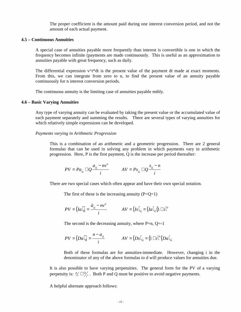
This is a combination of an arithmetic and a geometric progression. There are 2 general formulas that can be used in solving any problem in which payments vary in arithmetic progression. Here, P is the first payment, Q is the increase per period thereafter:

i

nvaQPaPV

n

n

n

−+= |

|

i

nsQPsAV n

n

−+= |

|

There are two special cases which often appear and have their own special notation. The first of these is the increasing annuity (P=Q=1)

( )i

nvaIaPV

n

nn

−== |

|

ɺɺ

( ) ( ) ( )nnn iIaIsAV +== 1||

The second is the decreasing annuity, where P=n, Q=-1

( )i

anDaPV n

n|

|

−== ( ) ( ) ( ) || 1 n

nn DaiDsAV +==

Both of these formulas are for annuities-immediate. However, changing i in the denominator of any of the above formulas to d will produce values for annuities due.

It is also possible to have varying perpetuities. The general form for the PV of a varying perpetuity is: 2i

Qi

P + . Both P and Q must be positive to avoid negative payments.

A helpful alternate approach follows:

- 16 -

Let == n

n vF the present value of a payment of 1 at the end of n periods. Let

== dv

nnG the present value of a level perpetuity of 1 per period, first payment at the

end of n periods. Finally, let == 2dv

nnH the present value of an increasing

perpetuity of 1, 2, 3, …, first payment at the end of n periods. By appropriately describing the pattern of payments, expressions for the annuity can be immediately written down.

Payments Varying in Geometric Progression

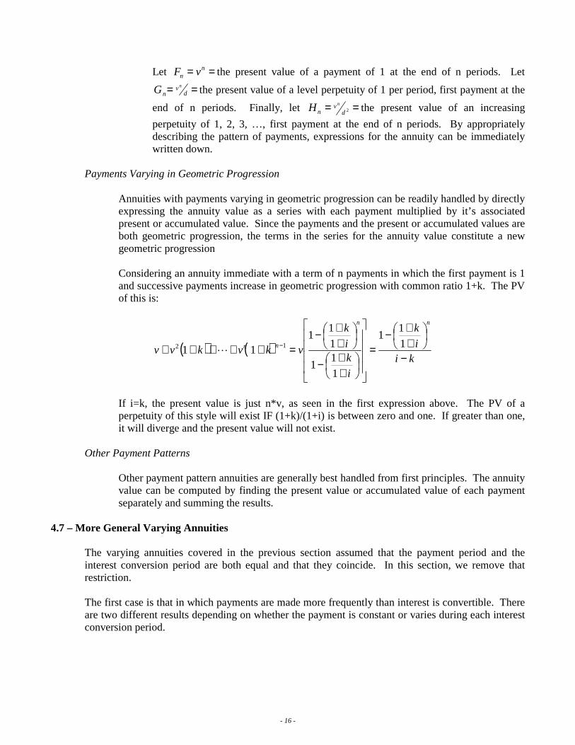
Annuities with payments varying in geometric progression can be readily handled by directly expressing the annuity value as a series with each payment multiplied by it’s associated present or accumulated value. Since the payments and the present or accumulated values are both geometric progression, the terms in the series for the annuity value constitute a new geometric progression Considering an annuity immediate with a term of n payments in which the first payment is 1 and successive payments increase in geometric progression with common ratio 1+k. The PV of this is:

( ) ( )ki

i

k

i

ki

k

vkvkvv

nn

nn

−

++−

=

++−

++−

=+++++ − 11

1

11

1

11

111 12

⋯

If i=k, the present value is just n*v, as seen in the first expression above. The PV of a perpetuity of this style will exist IF (1+k)/(1+i) is between zero and one. If greater than one, it will diverge and the present value will not exist.

Other Payment Patterns

Other payment pattern annuities are generally best handled from first principles. The annuity value can be computed by finding the present value or accumulated value of each payment separately and summing the results.

4.7 – More General Varying Annuities

The varying annuities covered in the previous section assumed that the payment period and the interest conversion period are both equal and that they coincide. In this section, we remove that restriction. The first case is that in which payments are made more frequently than interest is convertible. There are two different results depending on whether the payment is constant or varies during each interest conversion period.

- 17 -

When the rate of payment is constant in each period (in the first period, payments are 1/m, in the second they are 2/m, etc.), we develop the PV formula for an n-period annuity-immediate, payable

mthly: ( )( )( )m

n

nm

n i

nvaIa

−= |

|

ɺɺ

When the rate of payment changes with each payment period (1/m after the first mth, 2/m after the

2nd mth, etc.), the PV of the annuity becomes: ( )( )( )( )

( )m

nm

nm

nm

i

nvaaI

−= |

|

ɺɺ

4.8 – Continuous Varying Annuities

These annuities are primarily of theoretical interest, as they involve payments being made continuously, but at a varying rate. First, considering an increasing annuity. For n interest periods, where payments are being made continuously at the rate of t per period at time t. The differential expression t*v^t*dt is the present value of the payment t*dt made at exact moment t. Integrating this expression over zero to n gives

the PV of the annuity, denoted by ( ) |naI

In general, if the amount of the payment being made at exact moment t is f(t)*dt, simple replace t with the function in the integral just discussed. Even more generalized would be a situation in which the payments are being made continuous and the variations are occurring continuously, but also with the force of interest varying continuously.

- 18 -

Chapter 5 – Yield Rates 5.1 – Introduction

In this chapter, we present a number of important results for using the theory of interest in more complex “real-world” contexts than considered in the earlier chapters.

5.2 – Discounted Cash Flow Analysis

Extending the study of annuities to any pattern of payments, we come up with discounted cash flow analysis. We define C sub n as a deposit or contribution into an investment at time n. For convenience, assume that times of payments are equally spaced. Denote the returns or withdrawals from the investment as R sub n. It is obvious that contributions and returns are equivalent concepts viewed from opposite sides of the transaction, so R sub n = -C sub n. Assume that the rate of interest per period is i. Then, the net present value at rate i of investment

returns by the discounted cash flow technique is denoted by ( ) ∑=

=n

tt

t RviP0

. P(i) can be positive or

negative, depending on the interest rate. The yield rate is that rate of interest at which the present value of returns from the investment is equal to the present value of contributions into the investment. This can also be known as the internal rate of return. If we are dealing with two-party transactions, we can easily adopt the vantage point of either the borrower or the seller. To switch perspectives, simply change the signs of C-sub-t and R-sub-t. In this case, the value of the yield rate will remain unchanged. This manes that the yield rate on a transaction is determined by the cash flows defined in the transaction and their timing, and is the same from the perspective of either the borrower or the lender. From the lender’s perspective, the higher the yield rate the more favorable the transaction. Obviously this is opposite from the borrowers perspective. Yield rates are not necessarily positive. If it is zero, then the investor received no return on the investment, and if it is negative, then the investor lost money on the investment. Another important consideration in using yield rates is to consider the period of time involved. It is valid to use yield rates to compare alternative investments only if the period of investment is the same for all the alternatives. Obviously, all of the above results can be extended to include other regular (non-integral) or irregular intervals as well. If the payments constitute a basic annuity, use the same techniques as 3.8. In other situations, the easiest way to solve such problems would be to use the cash flows worksheet on financial calculators.

5.3 – Uniqueness of the Yield Rate

- 19 -

Transactions are occasionally encountered in which a yield rate is not unique. This is obvious, when you consider the formula for P(i) found in the last section. It’s a n’t degree polynomial in v, and is an nth polynomial in i if you multiply both sides by (1+i)^n. This has n roots. Because of the wide use of the yield rate, it is important to be able to ascertain whether or not the yield rate is unique. The yield rate will definitely be unique when all cash flows in one direction are made before the cash flows in the other direction. Descartes’ rule of signs will give us an upper bound on the number of multiple yield rates which may exist. The maximum number of yield rates is equal to the number of sign changes in the cash flows. If the outstanding investment balance is positive at all points throughout the period of investment, then the yield rate will be unique. Consequently, if the outstanding balance ever becomes negative at any one point, then a yield rate is not necessarily unique. It is also possible that no yield rate exists, or than all yield rates are imaginary.

5.4 – Reinvestment Rates

Prior to this point, we have had the implicit assumption that the lender can reinvest payments received from the borrower at a reinvestment rate equal to the original investment rate. If the lender is not able to reinvest the payments from the borrower at rates as high as the original investment, then the overall yield rate considering reinvestment will be lower than the stated yield rate. Oppositely, if the lender is able to reinvest the payments at even higher rates, then the overall yield rate will be higher than that stated. The consideration of reinvestment rates in financial calculates has become increasingly important and more widely used than ever. An important consideration to a lender is the rate of repayment by the borrower. The faster the rate of repayment, the more significant the reinvestment issue becomes. The slower the rate of repayment, the longer the initial investment rate will dominate the calculation. The results of financial calculations involving reinvestment rates are dependent upon the period of time under consideration. It is important to specify the period of time for which calculations are being made when reinvestment rates are being taken into account.

5.5 – Interest Measurement of a Fund In this section we devise a method to determine reasonable effective rates of interest. Make the following definitions: A = amount in fund at the beginning of the period B = amount in fund at the end of the period I = amount of interest earned during the period C sub t = the net amount of principal contributed at time t (0<=t<=1)

- 20 -

C = the total net amount of principal contributed during the period (C = SUM(Ct)) Obviously from these definitions: B = A + C + I For consistency, we assume that all of the interest earned is received at the end of the period.

We develop an approximation for i. ( )∑ ++≈

tt tCA

Ii

1. The denominator of this equation is the

average amount of principal invested, and is called the exposure associate with i. This does not produce a true effective rate of interest (we made a simple interest assumption in the development), it will be a good approximation as long as the Ct’s are small in relation to A. If this is not the case, then the error may become significant. A further simplifying assumption is often made. We assume that principal deposits and withdrawals occur uniformly throughout the period. So, on average, we assume that all transactions take place at time t=.5. This gives us further development:

( ) IBA

I

IABA

I

CA

Ii

−+≈

−−+≈

+≈ 2

5.5.

If it is known that on average, principal contributions occur at time k, not time .5, we can

use: ( ) ( )IkbkkA

Ii

−−−+≈

11, which reduces to the above if k=.5.

5.6 – Time-Weighted Rates of Interest

The methods considered in the previous section are sensitive to the amounts of money invested during various sub-periods when the investment experience is volatile during the year. Because of this, the rates computed by the methods in 5.5 are sometimes called dollar-weighted rates of interest. An alternative basis for calculating fund yields is called time-weighted rates of interest. Yield rates computed by the time weighted method are not consistent with an assumption of compound interest, however, they do provide better indicators of underlying investment performance than dollar-weighted calculations, however, the dollar-weighted ones provide a valid measure of the actual investment results achieved.

5.7 – Portfolio Methods and Investment Year Methods

These methods are used in situations in which an investment fund is being maintained for a number of different entities. An issue arises in connection with the crediting of interest to the various accounts. The two methods that are in common use are the portfolio methods and the investment year methods. Under the portfolio method, an average rate based on the earnings of the entire fund is computed an credited to each account. This is very straightforward and easy to implement. However, there are problems using this method during periods of fluctuating interest rates. There can be significant disincentives for new deposits into the fund, and an increased incentive for withdrawals if there has been a significant rise in interest rates in the recent past.

- 21 -

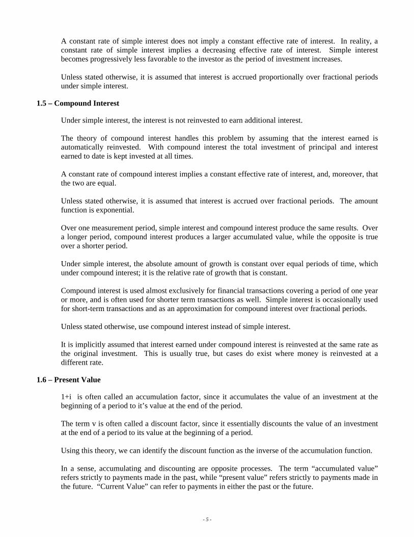
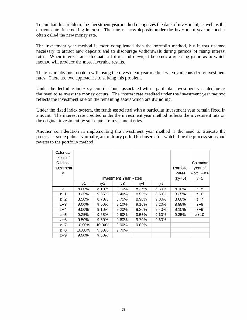
To combat this problem, the investment year method recognizes the date of investment, as well as the current date, in crediting interest. The rate on new deposits under the investment year method is often called the new money rate. The investment year method is more complicated than the portfolio method, but it was deemed necessary to attract new deposits and to discourage withdrawals during periods of rising interest rates. When interest rates fluctuate a lot up and down, it becomes a guessing game as to which method will produce the most favorable results. There is an obvious problem with using the investment year method when you consider reinvestment rates. There are two approaches to solving this problem. Under the declining index system, the funds associated with a particular investment year decline as the need to reinvest the money occurs. The interest rate credited under the investment year method reflects the investment rate on the remaining assets which are dwindling. Under the fixed index system, the funds associated with a particular investment year remain fixed in amount. The interest rate credited under the investment year method reflects the investment rate on the original investment by subsequent reinvestment rates Another consideration in implementing the investment year method is the need to truncate the process at some point. Normally, an arbitrary period is chosen after which time the process stops and reverts to the portfolio method.

Calendar Year of Original

Investment y

Portfolio Rates (i(y+5)

Calendar year of

Port. Rate y+5

iy1 iy2 iy3 iy4 iy5z 8.00% 8.10% 9.10% 8.25% 8.30% 8.10% z+5

z+1 8.25% 9.85% 8.40% 8.50% 8.50% 8.35% z+6z+2 8.50% 8.70% 8.75% 8.90% 9.00% 8.60% z+7z+3 9.00% 9.00% 9.10% 9.10% 9.20% 8.85% z+8z+4 9.00% 9.10% 9.20% 9.30% 9.40% 9.10% z+9z+5 9.25% 9.35% 9.50% 9.55% 9.60% 9.35% z+10z+6 9.50% 9.50% 9.60% 9.70% 9.60%z+7 10.00% 10.00% 9.90% 9.80%z+8 10.00% 9.80% 9.70%z+9 9.50% 9.50%

Investment Year Rates

- 22 -

EXAMPLE: An investment of $1000 is made at the beginning of calendar year z+4 in an investment fund crediting interest according to the rates in the table above. How much interest is credit in calendar years z+7 through z+9 inclusive? $1000*(1.09)*(1.091)*(1.092)=$1298.6 = accum. value at z+7 $1000(1.09)(1.091)(1.092)(1.093)(1.094)(1.091) = $1694.09 accum. value at z+9 1694.09-1298.6=395.49

- 23 -

Chapter 6 – Amortization Schedules and Sinking Funds 6.1 – Introduction In this section, 2 methods of repaying a loan are considered:

a. The Amortization Method: In this method the borrower repays the lender by means of installment payments at periodic intervals. This process is called “amortization” of the loan.

b. The Sinking Fund Method: In this method the borrower repays the lender by means of

one lump-sum payment at the end of the term of the loan. The borrower pays interest on the loan in installments over this period. It is also assumed that the borrower makes periodic payments into a fund, called a “sinking fund,” which will accumulate to the amount of the loan to be repaid at the end of the term of the loan

6.2 – Finding the Outstanding Loan Balance

When using the amortization method, the payments form an annuity whose present value is equal to the original amount of the loan. There are two approaches used in finding the amount of the outstanding balance, the prospective and the retrospective method.

In the prospective method, the outstanding loan balance at any point in time is equal to the present value at that date of the remaining payments. Under the retrospective method, the outstanding loan balance at any point is equal to the original amount of the loan accumulated to that date less the accumulated value at that date of all payments previously made. In general, the prospective and retrospective methods are equivalent. Symbol definitions: Outstanding loan balance at time t (after making the tth payment) =

|tn

pt aB

−= under the prospective

method, and ( )||

1t

t

n

rt siaB −+= . It can be shown that these are equal.

If the size and the number of payments are known, then the prospective method is usually more efficient. On the other hand, if the number of payments or the size of a final irregular payment is not known, then the retrospective method is usually more efficient.

6.3 – Amortization Schedules

An amortization schedule is a table which shows the division of each payment into principal and interest, together with the outstanding loan balance after each payment is made. If it is desired to find the amount of principal and interest in one particular payment, it is not necessary to construct the entire amortization schedule. The outstanding loan balance at the beginning of the period in question can be determined by either the retrospective or the prospective methods, and then that one line of the schedule can be created. In a perpetuity, the entire payment represents interest, therefore the outstanding balance always remains unchanged.

- 24 -

In the discussion of amortization tables, we made the following assumptions:

• Constant rate of interest • Annuity payment period and interest conversion period are equal • Annuity payments are level

6.4 – Sinking Funds

In many cases, the borrower will accumulate a fund which will be sufficient to exactly pay off the loan at the end of a specified period of time, paying off the loan in one lump-sum payment, rather than as an annuity stream. This fund is called a “sinking fund.” We are primarily interest in the cases where the payments into the sinking fund follow a regular pattern (where they are some form of an annuity). Usually, the borrower pays interest on the load periodically, called “service” on the loan. Since these are interest only payments, the outstanding balance of the loan remains constant. Because the balance in the sinking fund could be applied against the loan at any point, the net amount of the loan is equal to the original amount of the loan minus the accumulated value of the sinking fund. If the rate of interest on the loan equals the rate of interest earned on the sinking fund, then the sinking fund method is equivalent to the amortization method. Now we consider the situation in which the interest rate on the loan and the interest rate earned on the sinking fund differs. The rate on the loan is denoted by i, and the rate on the sinking fund is denoted by j. Usually, j is less than (or equal to) i. The total payment is split into two parts. Interest at rate i will be paid on the amount of the loan. The remainder of the total payment not needed for interest will be placed into a sinking fund accumulating at rate j. In general, the sinking fund schedule at two rates of interest is identical to the sinking fund schedule at one rate of interest equal to the rate of interest earned on the sinking fund, except that a constant addition of (i-j) times the amount of the loan is added to the interest paid column.

6.6 – Varying Series of Payments

In this section, we consider more general patterns of payment variation. We will continue to assume that the interest conversion period and the payment period are equal and will coincide.

∑=

=n

it

t RvL1

If you wish to construct an amortization schedule, it is easy to prepare from first principles, or the outstanding loan balance column can be found retrospectively or prospectively, from which the remaining columns can be found.

- 25 -

One common pattern of variation is that in which the borrow makes level payments of principal. Clearly, this leads to successive total payments (consisting of interest and principal) to decrease. It is possible that when using varying payments, the interest due in a payement is larger than the total payment. In this case, the principal repaid would be negative, and the outstanding balance of the loan would increase! The increase in the outstanding balance arises from interest deficiencies being capitalized, and added to the amount of the loan, in what is called negative amortization.

- 26 -

Chapter 7 – Bonds and Other Securities 7.1 – Introduction There are 3 main questions that this chapter will consider:

(1) Given the desired yield rate of an investor, what price should be paid for a given security?

(2) Given the purchase price of a security, what is the resulting yield rate to an investor? (3) What is the value of a security on a given data after it has been purchased?

7.2 – Types of Securities

Bonds

A bond is an interest bearing security which promises to pay a stated amount (or amounts) of money at some future date (or dates). They are commonly issued by corporations and governmental units as a means of raising capital. Bonds are generally redeemed at the end of a fixed period of time (the end of the bonds term). The end of the term is the maturity date. Bonds with an infinite term are called perpetuals. Bonds may be issued with a term which varies at the discretion of the borrower. These are called callable bonds. Any date prior to, or including, the maturity date on which a bond may be redeemed is termed a redemption date. Coupons are periodic payments made by the issuer of the bond prior to redemption. On an accumulation bond, the redemption price includes the original loan plus all accumulated interest. Zero coupon bonds have recently become very popular. However, most bonds do have periodically payable coupons, and this will be assumed unless otherwise stated. Accumulation or zero coupon bonds can be easily handled with compound interest methods already discussed. A second classification is the distinction between registered bonds and unregistered bonds. A registered bond is one in which the lender is listed in the records of the borrower. If the lender decides to sell the bond, the change must be reported to the borrower. The coupon payments are paid by the borrower to the owners of record on each coupon payment date. An unregistered bond is one in which the lender is not listed in the records of the borrower. In this case, the bond belongs to whomever gas legal possession of it. They are generally called bearer bonds, and are occasionally called coupon bonds, due to the physically attached coupons. A third classification that can be made is according to the type of security behind the bond.

o A mortgage bond is a bond secured by the mortgage on a real property. o A debenture bond is one secured only by the general credit of the borrower.

In general, mortgage bonds possess a higher degree of security that debenture bonds, since the lenders can foreclose on the collateral in the even of the default of a mortgage bond.

- 27 -

Income bonds have largely disappeared over recent years, but they are a type of high risk bond in which coupons are paid only if the borrower has earned sufficient income to pay them. A more modern high-risk bond is often called a “junk” bond. They have a significantly higher risk of default in payments than corporate bonds in general. Because of this, they must pay commensurately higher rates of interest to the lender for assuming the risk. A convertible bond is a sort of ‘hybrid’ bond. This can be converted into the common stock of the issuing corporation at some future date under certain conditions. This is the choice of the owner of the bond. These bonds are generally debenture bonds.

Preferred Stock

This is a type of security which provides a fixed rate of return (similar to bonds). However, unlike bonds, it is an ownership security (bonds are debt security). Generally, preferred stock has no maturity date, although on occasion preferred stock with a redemption provision is issued. The periodic payment is called a dividend, because it’s being paid to an owner. Preferred stock ranks behind bonds and debt securities, since payments on indebtedness must be made before the preferred stock receives a dividend. Preferred stock is ranked ahead of common stock, however. Some corporations have issued cumulative preferred stock, to increase the degree of a security. In these, any dividends the corporation is unable to pay are carried forward to future years (where they presumably will). All arrears on preferred stock must be paid before any dividends on common stock can be paid. Stocks that receive a share of earnings over and above the regular dividend if earnings are at a sufficient level are called participating preferred stock. Convertible preferred stock has a privilege similar to convertible bonds. Owners have the option to convert their preferred stock to common stock under certain conditions.

Common Stock

Common stock is another type of ownership security. It does not earn a fixed dividend rate as preferred stock does. Dividends on this type of stock are paid only after interest payments on all bonds and other debt and dividends on preferred stock are paid. The dividend rate is flexible, and is set by the board of directors at its discretion.

Because of the volatility of common stock dividend rates, the prices are much more volatile than either bonds or preferred stock. All residual profits after dividends to the preferred stockholders belong to the common stock holders.

7.3 – The Price of a Bond When considering the price of a bond, we make the following assumptions

- 28 -

a. All obligations will be paid by the bond issuer on the specified dates of payments. We ignore any possibility of default in this chapter

b. The bond has a fixed maturity date. Bonds with no maturity date are equivalent to preferred stock.

c. The price of the bond is desired immediately after a coupon payment date (we will consider the price between two coupon dates later.

Bond Symbols & Notation: P = the price of a bond F = par value/face amount of a bond C = the redemption value of a bond (the amount of money paid at a redemption date to the holder of the bond) Sometimes C is equal to F. It is possible for C to differ from F in 2 cases: (1) a bond which matures for an amount not equal to it’s par value, or (2) a bond which has a redemption date prior to the maturity date on which a bond is redeemed for an amount not equal to its par value. Assume that a bond is redeemable at par unless told otherwise. r = the coupon rate of the bond (the rate per coupon payment period used in determining the amount of the coupon. It is assumed that coupons are constant. Fr = amount of the coupon g = modified coupon rate. g=Fr/C. The coupon rate per unit of redemption value (r is the coupon rate per unit of par value. When F=C, g=r. g is convertible at the same frequency as r. i = the yield rate of a bond, or the yield to maturity. The interest rate actually earned by the investor, assuming the bond is held until redemption or maturity. Equivalent to the IRR. It is assumed that the yield rate is constant. n = the number of coupon payment periods from the date of the calculation to the maturity date, or to a redemption date K = the present value, computed at the yield rate, of the redemption value at the maturity date, or a redemption date G = the base amount of a bond. Gi=Fr � G=Fr/i. G is the amount which, if invested at the yield rate I, would produce periodic interest payments equal to the coupons on the bond. There are 3 different types of yields associated with a bond.

1. “Nominal Yield” is the annualized coupon rate on a bond 2. “Current Yield” is the ratio of the annualized coupon to the original price of the

bond. The current yield does not reflect any gain or loss when the bond is sold, redeemed, or matures.

3. “Yield to Maturity” is the actual annualized yield rate, or internal rate of return.

F, C, r, g, and n are given by the terms of a bond and remain fixed throughout the bonds life. P and I will vary throughout the life of the bond. Price and yield rate have a precise inverse relationship to each other. There are 4 types of formulas which can be used to find the price of a bond. First of these is the basic formula. According to this method, the price MUST be equal to the present value of future coupons plus the present value of the redemption value: KFraCvFraP

n

n

n+=+=

||

The second formula is the premium/discount formula, and is derived from the basic formula:

- 29 -

( ) ( )

||||1

nnn

n

naCiFrCiaCFraCvFraP −+=−+=+=

The third, the base amount formula, can also be derived from the first formula: ( ) ( ) nnnn

n

n

nvGCGCvvGCvGiaCvFraP −+=+−=+=+= 1

||

The fourth, the Makeham formula, is also obtained from the basic formula:

( )KCi

gKCvC

i

gCv

i

vCgCvFraCvP nn

nn

n

n −+=−+=

−+=+= 1|

7.4 – Premium and Discount

If P>C, the bond is said to sell at a premium, and the difference between P and C is called the “premium.” Likewise, if P<C, then the bond sells at a discount, and the difference between C and P is called the “discount.” Premium and discount are essentially the same concept, since discount is merely a negative premium. These represent the cases in which F != C. Since the purchase price of a bond is usually less than or greater than the redemption value, there will be a profit or a loss at the redemption date. This profit or loss is reflected in the yield rate for the bond, when calculated as the yield to maturity. Because of this profit or loss at redemption, the amount of each coupon CANNOT be considered as interest income to an investor. It is necessary to divide each coupon into interest earned and premium adjustment portions similar to the separation of payments into interest and principle when discussing loans in the previous chapter. When using this approach, the bond’s value will be continually adjusted from the price on the purchase date to the redemption value on the redemption date. Adjusted values of the bond are called the book values. They provide a reasonable and smooth series of values for bonds, and are used by many investors in reporting the asset values of bonds for financial statements. The book value after purchase will differ from the price if the bond is newly bought. The price of the bond in the market will vary with changes in the prevailing interest rate, while the book values will follow a smooth progression (since they are based on the locked in yield rate at purchase). A bond amortization schedule is a table which shows the division of each coupon into its interest earned and principal adjustment portions, together with the book value after each coupon is paid. To illustrate, we consider a basic, simplified bond, with C=1, P=1+p (p is the premium/discount, and can be positive or negative), and the coupon is equal to g. At the end of the first coupon period the interest earned on the balance at the beginning of the period is: ( )[ ]

inaigiI

|1 1 −+= . The rest of the

total coupon of g must be used to adjust the book value. The rest of the coupon: ( ) nvigIgP −=−= 11 . The book value at the end of the period equals the book value at the

beginning of the period minus the principal adjustment amount:

- 30 -

( )[ ] ( ) ( )in

n

inaigvigaigB

|1|1 11−

−+=−−−+= . The same reasoning can be used to expand this to

other lines of the schedule. The book values agree with the price of a bond given by the second method in the previous section, computed at the original yield rate. The sum of the principal adjustment column is equal to p, the amount of premium or discount. The sum of the interest paid column is equal to the difference between the sum of the coupons and the sum of the principal adjustment column. The principal adjustment column is a geometric progression with common ratio (1+i). therefore, knowing any other principal adjustment amount and the yield rate allows you to know any other principal adjustment amount. When a bond is bought at a premium, the book value will gradually adjust downward, through amortization of premium (or writing down). In these cases, the principal adjustment is often called the “amount for amortization of premium.” When a bond is bought at a discount, the book value will gradually be adjusted upward. This is called accumulation of discount, or writing up. Here, the principal adjustment amount is called the “amount for accumulation of discount.” Be careful to ascertain in any bond amortization schedule whether the bond is selling at a premium or a discount, as negative numbers are usually avoided in the tables. Much like dealing with loans, if it is desired to find the interest earned or principal adjustment portion of any one coupon, it is not necessary to construct the entire table. Simply find the book value at the beginning of the period in question (which is equal to the price at that point computed at the original yield rate), and then find that one line of the table. Another method of writing up or writing down the book values of bonds is the straight line method. This does not produce results consistent with compound interest, but it is very simple to apply. In this method, book values are linear, grading from P=B(0) to C=B(n). This leads to a constant principal adjustment column. The interest earned column is also constant. Clearly, the larger the amount of premium or discount, and the longer the term of the bond, the greater the error in using this method will be.

7.5 – Valuation Between Coupon Payment Dates

If tB and 1+tB are the book values or prices of a bond on two consecutive coupon dates, and Fr is the

amount of the coupon, the follow recursive relationship holds: ( ) FriBB tt −+=+ 11 , assuming a

constant yield rate over the interval. When a bond is bought between coupon dates, it is nrcessary to allocate the coupon for the current period between the prior owner and the new owner. Obviously, the new owner will receive the entire coupon at the end of the period, so the purchase price should include a payment to the prior owner for the portion of the coupon that is earned while in the prior owners possession. This value is called the accrued coupon, and is denoted by kFr .

Define the flat price of a bond as the money which actually changes hands at the date of the sale (ignoring expenses), and denote this by f

ktB + . Define the market price of a bond as the price

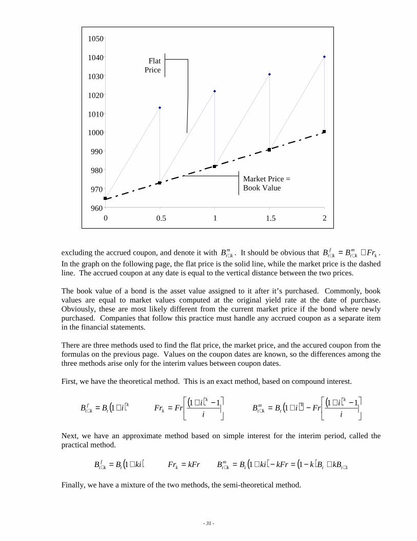
- 31 -

excluding the accrued coupon, and denote it with mktB + . It should be obvious that k

mkt

fkt FrBB += ++ .

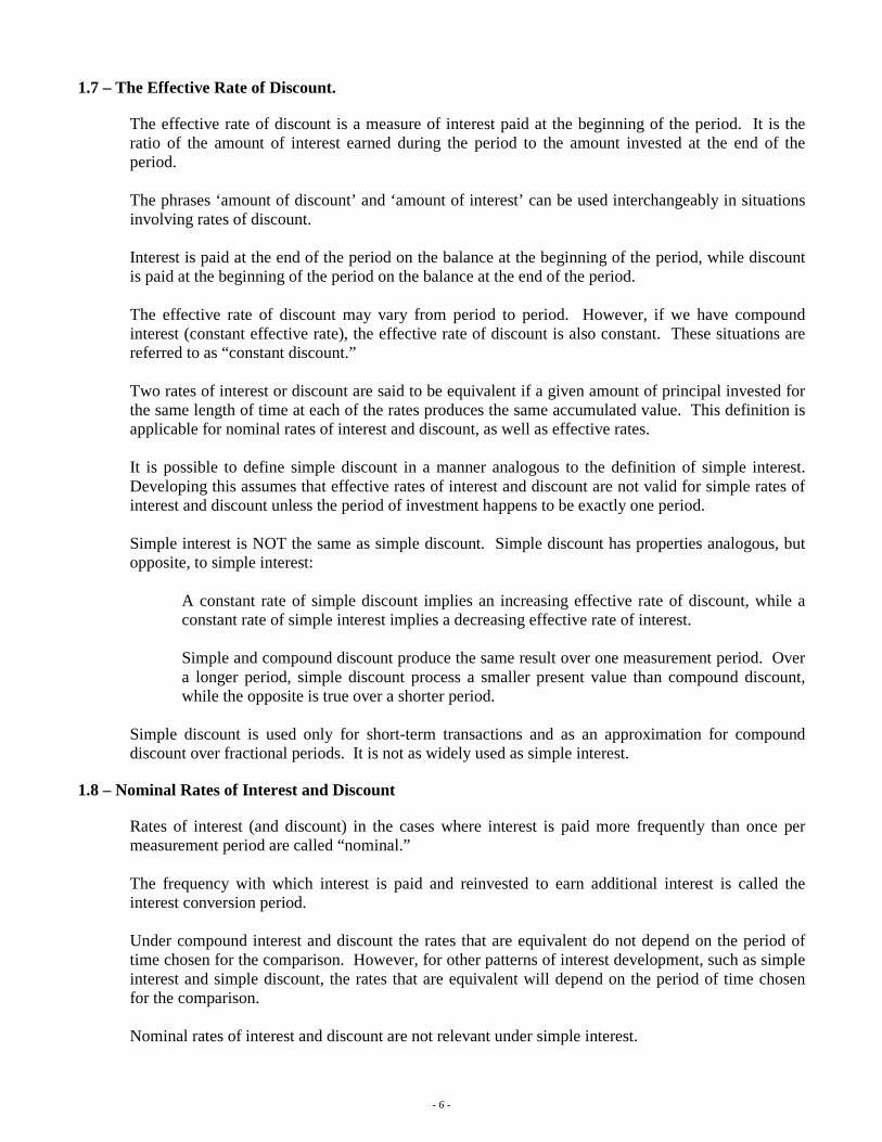
In the graph on the following page, the flat price is the solid line, while the market price is the dashed line. The accrued coupon at any date is equal to the vertical distance between the two prices. The book value of a bond is the asset value assigned to it after it’s purchased. Commonly, book values are equal to market values computed at the original yield rate at the date of purchase. Obviously, these are most likely different from the current market price if the bond where newly purchased. Companies that follow this practice must handle any accrued coupon as a separate item in the financial statements.

There are three methods used to find the flat price, the market price, and the accured coupon from the formulas on the previous page. Values on the coupon dates are known, so the differences among the three methods arise only for the interim values between coupon dates. First, we have the theoretical method. This is an exact method, based on compound interest.

( )kt

fkt iBB +=+ 1

( )

−+=i

iFrFr

k

k

11 ( ) ( )

−+−+=+ i

iFriBB

kk

tm

kt

111

Next, we have an approximate method based on simple interest for the interim period, called the practical method.

( )kiBB tf

kt +=+ 1 kFrFrk = ( ) ( ) 111 ++ +−=−+= tttm

kt kBBkkFrkiBB

Finally, we have a mixture of the two methods, the semi-theoretical method.

960

970

980

990

1000

1010

1020

1030

1040

1050

0 0.5 1 1.5 2

Flat Price

Market Price = Book Value

- 32 -

( )kt

fkt iBB +=+ 1 kFrFrk = ( ) kFriBB k

tm

kt −+=+ 1

There is a flaw in the semi-theoretical method, however. If P=C, there is no amortization of premium or accumulation of discount, so the book values on all the coupon dates are equal. Clearly, it would make sense that all interim book values should also be equal to that same value. This is true under the first two methods, but fails under the semi-theoretical method. Still, the semi-theoretical method is the most widely used in practice. The graph on the previous page shows the practical methods. Graphs showing the other methods would be similar, and the values on the coupon payment dates would be identical. One final issue is the amount of premium or discount between coupon payment dates. These values should be based on the market price or book value rather than on the flat price.

Premium CB m

kt −= + and Discount mktBC +−=

7.6 – Determination of Yield Rates

The determination of the yield to maturity on a bond is similar to the determination of an unknown rate of interest for an annuity. One approach is linear interpolation in bond tables. Another approach is to develop approximation formulas for the yield rate via algebra. Two main formulas that have been developed are:

kn

nn

kg

i

2

11

++

−≈ and

k

n

kg

i

2

11+

−≈ . The second of these formulas is the bond salesman’s method.

Again, like with previous sections, you can use iteration, but that seems useless to spend time learning for this exam. Consider the situation in which a bond is purchased for P, coupons of Fr are paid at the end of each period for n periods, the bond is redeemed for C at the end of n periods, and the coupons are reinvested at rate j. Denoting the yield rate considering reinvestment by i’, we would have the

equation of value: ( ) CFrsiPjn

n +=′+|

1

This is the reasoning behind the popularity of zero coupon bonds. Since there are no coupons to reinvest, the yield rate is locked-in at the date of purchase.

7.7 – Callable Bonds

A callable bond is a bond in which the borrower has an option to redeem prior to it’s maturity date. The earliest call date is usually several years after the issue date. Callable bonds present a problem when calculating prices and yields, because the term (n) is unknown. Since the borrower has an option whether or not to call the bond, the investor should

- 33 -

assume that the borrower will exercise that option to the disadvantage of the investor, and should calculate the yield rate and/or price accordingly. If the redemption values on all the redemption dates (including the maturity date) are equal, the principle is easy to apply, and the following rules hold:

1. If the yield rate is less than the modified coupon rate (if the bond sells at a premium), then assume that the redemption date will be the earliest possible date. There will be a loss at redemption, and the most unfavorable situation occurs when the bond was bought at a premium.

2. If the yield rate is greater than the modified coupon rate (if the bond sells at a discount), then assume that the redemption date will be the earliest possible date. There will be a gain at redemption, and the most unfavorable situation occurs when the gain is as late as possible.

If the redemption values on all the redemption dates are not equal, this principle is a little harder to apply. The most unfavorable date will not necessarily be either the earliest or the latest possible date. Remember that the most unfavorable call date is the one that produces the smallest purchase price at the investors yield rate. If a callable bond is redeemed at a date other than that assumed initially, the yield rate his higher than originally calculated. However, in this situation, the original purchase price and the term are both fixed. The above discussion has ignored reinvestment rates. This should concern us, since we are comparing yield rates over different periods of time. Using yield rates to compare transactions over different periods of time may result in a flawed comparison.

7.10 – Other Securities

Preferred Stock and Perpetual Bonds

These are both types of fixed-income securities without redemption dates. The price must be equal to the present value of future dividends or coupons forever, so the payments form a perpetuity. Be aware that some preferred stock is issued with a redemption date. In these cases, it can be treated exactly like a regular bond.

Common Stock

Common stock is not a fixed-income security, as its dividends are not known in advance, nor are they level. In theory, common stock prices should represent the present value of future dividends. Values computed in this fashion are based on the dividend discount model. This calculation should take into account projected changes in the dividend scale.

The theoretical price of the stock is ki

DP−

= 1, where D is the dividend at the end of the

current period, k is re rate that dividends are projected to change (geometrically), and i is the rate per period that the stock is purchased to yield.

- 34 -

It is unrealistic to project constant percentage increases in dividends indefinitely into the future. As corporations increase in size and become more mature, the rate of growth will generally slow down. This can be taken into account in the model above.

- 35 -

Chapter 8 – Practice Applications 8.7 – Short Sales

Investors in securities use short sales, or short transactions when they think the price of a security is likely to decline. In short sales, the sale occurs first and the purchase occurs later. In this context, normal transactions (purchase first) are called long transactions. With a short sale, the investor borrows the security from a second party and sells it in the market to a third party. At some later date, the investor buys back the security in the market, in order to return it to the second party. Buying back the security is “covering the short.” One problem with short sales is determining the yield rate. If the transactions occurs exactly as stated, the yield rate does not exist. Some say the yield rate is infinite, since there was profit made on no real investment. However, short sales rarely occur as defined above. In practice, the short seller is required to make a deposit of a percentage of the price at the time the short sale is made. This deposit is called the margin, and cannot be recovered by the short seller until the short position is covered. The short seller will be credited with interest on the margin deposit, which will increase the yield rate. The short seller is not allowed to earn interest on the proceeds from the short sale. Governmental regulations require that these proceeds remain in a non-interest bearing account until the short position is covered, at which time these funds will be used for the purchase necessary to cover the short. Any leftover money is profit on the transaction, while a negative balance would be loss on the transaction. If the short position develops a loss, additional margin may be required prior to the position being covered. Conversely, if the position develops a profit, part of the margin may be released and can be withdrawn or used for other purposes. If the security in question pays dividends or interest, then the short seller is required to pay these to the purchaser of the security. This will lower the yield rate realized. Investment strategies have been developed that involve combinations of long and short positions in related securities, which have greatly reduced risk and also have a good prospect to earn a reasonable return on investment. A generic name for these transactions is “hedging.” Situations in which a profit is certain are called arbitrage. Arbitrage opportunities are rate, since market prices react quickly to eliminate them.

8.8 – Modern Financial Instruments

Money Market Funds

Money Market funds provide an investor a secure investment, with high liquidity and a fairly high yield. They occasionally provide check-writing facilities, making these accounts similar to checking accounts, only with a higher interest rate. Investments made by money market funds are in a variety of short-term, fixed-income investments, in both the government and the private sector. The rate credited on money market funds fluctuates because there is only a short-term investment made. They generally allow withdrawals on demand without

- 36 -

penalty, making them an ideal place to keep money while considering other investment opportunities.

Certificates of Deposit

CD’s are another short (to medium) term investment. They provide a specified rate of interest for a fixed period of time. There are long-term securities, but few of these have the fixed income rates of the shorter term CD’s. They are issued in a range of denominations, and higher denominations often earn a higher interest rate than the lower ones. CD’s have more stable rates than money markets, but at the cost of liquidity, as CD’s usually charge a penalty for early withdrawal. Often, this penalty is avoided by selling the CD on the secondary market. CD’s don’t fluctuate in value with movements in the interest rate, and they are FDIC guaranteed, up to $100k.

Guaranteed Investment Contracts (GICs)

GIC’s are investment instruments issued by insurance companies, usually to large investors such as pension funds. They guarantee principal and interest over a stated period of time (like CD’s), so their market value does not fluctuate with movements in the interest rate. GIC’s are different from CD’s in that they allow additional deposits during the first 3 months to a year. Like CD’s, withdrawals are restricted. Often they have annuity purchase options (when the GIC is being used for the investment of a pension fund). GIC’s pay higher rates of interest than CD’s, but they are not insured by the FDIC. They closely match yield rates on Treasury securities. Recently, banks have developed BICs, similar to GIC’s, but insured by the FDIC

Mutual Funds

Mutual Funds are pooled investment accounts, in which the individual investor buys shares, They offer a greater degree of diversification than individuals could achieve on their own. Originally, they where primarily invested in common stock, but more recently, they have expanded to a much broader array of other investment options. Considerable variation exists around various funds in their relative emphases on safety of principal, income, and growth.

Mortgage Backed Securities

MBSs are securities which are created out of a defined pool of real estate mortgages. Investors receive periodic payments consisting of both principal and interest. The rate at which the principal is repaid is variable, and dependant on the rate at which the underlying mortgages are paid off. The three corporations that issue MBSs:

1. The Government National Mortgage Association issues MBS called “Ginnie Maes.” Payment of principal and interest is guaranteed by the full faith and credit of the U.S. Government

2. The Federal Home Loan Mortgage Corporation issues MBS called “Freddie Macs.” The corporation (but not the government) guarantees payment of principal and interest.

3. The Federal National Mortgage Association issues MBS called “Fannie Maes.” The corporation, but not the government, guarantees payment of principal and interest.

- 37 -

Collateralized Mortgage Obligations

CMOs are new, designed to improve upon the traditional mortgage backed securities. They involve the same type of investment in real estate mortgages, but involve complex structuring of the portfolios designed to lessen the uncertainty in cash flow found in a typical MBS. They do not have a specific maturity date, and are sold on a basis which quotes their “average life.” This average life is the average amount of time that each dollar of principal is expected to be outstanding, assuming a reasonable prepayment schedule for the pool of mortgages. They are structured with a wide range in average life, providing more choice to the investor. CMOs offer higher yields than corporate bonds, in order to compensate for the uncertainty of their repayment schedule, and the attendant reinvestment risk. They feature either monthly or quarterly payments. They are very liquid, and their prices in the market vary inversely with prevailing interest rates (like bond prices).

- 38 -

Chapter 9 – More Advanced Financial Analysis 9.4 – Recognition of Inflations

Rates of interest are positively correlated with rates of inflation (over time, the two tend to move in the same direction. This is because inflation represents loss of purchasing power. Lenders will demand higher rates of interest in order to compensate for the loss of value in their capital. Borrowers will be willing to pay higher rates, to pay off their loans with the lessened value-dollar. In reality, the relationship is not between current interest rates and current inflation dates, it’s between current interest rates and the expected rate of inflation. The rate of interest eliminating inflation is called the real rate of interest, and is denoted by i’. The actual rate of interest is called the nominal rate of interest, and is denoted by i. This is not the same as the nominal rate of interest in 1.8 or 7.3, it merely means it is the rate of interest “in name only.” The rate of inflation is denoted by r, and is assumed to be constant.

( )( )rii +′+=+ 111 , which, solving for i, is ririi ′++′= . Since the cross product term is usually small, it is convenient for people to approximate the nominal rate of interest as the sum of the real rate of interest and the rate of inflation.

Rearranging the above for i’ gives i

ii

++=′+

1

11 , or

r

rii

+−=′

1. So, i’ will be relatively

stable over time, and i and r will tend to move up and down together. The relationship is not precise, and i’ is not totally constant over time, nor is the correlation between r and i exact either. The equations are ‘rules of thumb,’ not exact relationships. When computing present values of future payments:

1. If future payments are not affected by inflation, then discount at the nominal rate of interest 2. If future payments are adjusted to reflect the rate of inflation and the adjustment is reflected

in the payment amount, then also discount at the nominal rate of interest. 3. If future payments are adjusted to reflect the rate of inflation but the adjustment is not

reflected in the payment amount, the correct procedure is to discount at the real rate of interest.

9.6 – Yield Curves

Typically, at any point in time, the short and the long term rates of interest are different. This is called the term structure of interest rates. Typically, long term interest rates are higher than short term interest rates. Another phrase used to describe the term structure of interest rates is the yield curve. When rates increase with the length of the investment period, the yield curve has a positive slope. There are several theories as to why this upward slope develops in markets.

• The expectations theory says that a higher percentage of individuals and business firms have an expectation that interest rates will rise in the future than the percentage that expect them to fall.

• The liquidity preference theory states that individuals and firms prefer to invest for short periods rather than for long periods, so that they will have early access to their funds. An

- 39 -

increase in the long-term rate is necessary to get investors to commit their funds for longer periods of time.

• The inflation premium theory says that investors feel a significant amount of uncertainty about future rates of inflation, and will demand higher rates of interest on long term-investments. Higher rates of inflation leads to higher interest rates, depressing market values of investments. Long term assets are affected more than short term assets by movement in interest rates.

When short-term rates exceed long-term rates, the yield curve is inverted. Another pattern that may be encountered is that of a flat yield curve, at least over a major portion of the periods in the term structure. This happens in stable periods, when investors do not expect dramatic changes in investment markets (or the rate of inflation) in the future. Interest rates on the yield curve are called spot rates. Although most investments involve a mixture of payments at various points in time, it is relatively easy to determine spot rates. There are securities called stripped Treasuries that are created by separating the coupons from the redemption vales on Treasury securities. Then, these various coupons and redemption values are repackaged into a series of zero-coupon bonds, each with a different term. The yield rates on these bonds at any one point in time provides an immediate measure of the risk-free yield curve. One criticism of the internal rate of return (and NPV) is that it ignores the term structure of interest rates, assuming a constant interest rate throughout the entire period. Basically, the IRR calculation involves a complex averaging of many different spot rates from the yield curve. An alternate procedure that could be used is to discount each payment by its associated spot rate.

Then, a generalized equation for the NPV/IRR becomes: ( ) ( )∑=

−∗ +=

n

tt

tt RiiP

0

1 . The use of spot

rates is an important application of computing annuity values with varying rates of interest. Another type of interest rate is the forward rate. This is a spot rate that will come into play in the future. A forward rate can be thought of as a future reinvestment rate. For example, consider a firm with 2 options. The first option is to borrow money for 2 years at the 2 year spot rate of 10%. The second option is to borrow for one year at the one year spot rate of 8%, and to borrow for the second year at the one year spot rate in effect a year later. This 1-year spot rate for the next year is a forward rate.

This firm will be indifferent between the two options if ( ) ( )( )f+= 108.11.1 2 , which gives 12.=f . If the firm expects the forward rate to be greater than 12%, it should use the first option to borrow, but if they expect the forward rate to be less than 12%, it should use the second option to borrow. In referring to forward rates, we need to be precise in specifying the period of deferral and the period for which the rate applies. The use of spot rates and forward rates in the term sturtcure of interest rates gives us a more sophisticated way of analyzing alternatives for investing and borrowing, and is the basis for extensive hedging and arbitrage strategies.

9.8 – Duration

Obviously, the timing of future payments is important in the financial analysis word. Here, we develop some indices to measure the timing of future payments. The most basic of these is the term-

- 40 -

to maturity. For example, for 10 year bonds at issue, the term to maturity is 10. This index is of limited value, as it would not distinguish between 10 year bonds with differing coupon rates. A better index is the method of equated time, previously developed. This is the weighted average of the various times of payments, where the weights are the various amounts paid. It is the average term to maturity. If a series of R’s represent payments made at integral times, then we have:

∑

∑

=

=

⋅=

n

tt

n

tt

R

Rtt

1

1

An even better index is given by duration. This is similar to the method of equated time, but the

present value of each payment is used as the weight, instead of the payment itself:

∑

∑

=

=

⋅

⋅⋅=

n

tt

t

n

tt

t

Rv

Rvtd

1

1 .

Duration is a function of the interest rate. Note that if i=0, duration matches the method of equated time. Duration is a decreasing function of i. As the rate of interest increases, the terms in the numerator with the higher values of t are discounted more than the terms with the lower value of t. If there is only one future payment, duration is the point in time at which that payment is made. We also want to be able to examine the rate of change in the present value of a series of future

payments as the rate of interest changes. Recall that ( ) ( )∑=

−+=n

tt

tt RiiP

0

1 . Now, we define the

volatility of this present value as: ( )( )iP

iPv

′−= , where volatility is a function of i. Volatility is a

measure of how rapidly the present value of series of future payments changes as the rate of interest changes.

It can be shown that ( )( ) i

d

iP

iPv

+=

′−=

1. Because of this close relationship, volatility is often called

modified duration. Duration and modified duration provide an index of the average length of an investment. None of the results in this section are valid if the payment amounts vary depending on the interest rate.

9.9 – Immunization

Now, we consider the interrelationship between assets and liabilities for some financial enterprise, like a bank, insurance company, or pension fund. Clearly, assets generate a series of cash inflows, while liabilities generate a series of cash outflows. The issue is how to achieve an equilibrium or safe balance between inflows and outflows. If this equilibrium does not exist, there can be many problems that arise. The primary problem is the risk of adverse effects created by changes in the level of interest rates. A significant risk to a financial institution occurs if the assets backing their contacts are invested either too short or too long.

- 41 -

If the assets are invested too long, the financial institution is vulnerable to losses if interest rates rise. Contract holders are likely to withdraw their funds at the end of the year, and the institution may have to sell assets to pay the departing contract holders. However, because of the rise in the interest rates, the value of the assets that would have to be sold will have declined in value, resulting in losses for the firm. If the assets are invested too short, the financial institution is vulnerable to losses if interest rates fall. Since its assets would not be invested very short-term, interest earnings will decline quickly, and may not be sufficient to pay the guaranteed interest on contracts the institution may have sold. Therefore, there will be losses in this situation as well. Immunization is a technique designed to structure assets and liabilities in a manner that would reduce or eliminate these types of problems. Let the net receipt at time t be ttt LAR −= . Assume that the present value of the cash inflows from

the assets is equal to the present value of the cash outflows from the liabilities. Thus, we have P(i)=0. Now, we would like P(i) to have a local minimum at zero, so that small changes in the interest rate in either direction will increase the present value of the cash flows. In order to obtain this local minimum, we need P’(i)=0, and P”(i)=0.

The second derivative of P(i) is used to define convexity, as ( )( )iP

iPc

′′= .

Because liabilities are largely determined by forces outside the control of the company in question, immunization is aimed at managing the structure of the assets. The immunization strategy is to arrange the assets so that three conditions are met:

1. Present value of cash inflows from assets is equal to the present value of cash outflows from the liabilities. This assures that the correct amount of assets are utilized to support the liabilities.

2. The modified duration of the assets is equal to the modified duration of the liabilities. This ensures that the price sensitivity to changes in interest rates is the same for the assets and the liabilities.

3. The convexity of the assets is greater than the convexity of the liabilities. When this occurs, a decrease in interest rates will cause asset values to increase more than the increase in liability values, and when interest rates increase, asset values will decrease by less than the decrease in liability values.

There are still a number of problems with implementing an immunization strategy:

1. Different strategies may emerge depending on the value of i chosen, the choice of which is not always clear.

2. The technique is designed to work for small changes in i. There is no assurance that the process will continue to work for large changes in i.

3. The yield curve is not reflected in this technique. This technique assumes that the entire yield curve shifts in parallel when interest rates change. If there are other patterns, the theory breaks down. This is a common problem, as short term rates are often more volatile than long term rates

4. Immunization requires frequent rebalancing of portfolios to keep modified duration of assets and liabilities equal. Modified duration does not decrease by one year for each that elapses, but changes at different rates for different investments.

- 42 -

5. Exact cash flows may not be known, and may have to be estimated. 6. The convexity condition implies that a profit can be made with interest rate movements in

either direction. This violates a principle of finance theory which states that risk-free arbitrage does not exist for a significant period of time in efficient markets.

7. Assets may not exist in the right maturities to achieve immunization. This could happen if the modified duration of the liabilities is very long.

Even with these problems, partial immunization is superior in practice to not recognizing the relationship between assets and liabilities at all.

9.10 – Matching Assets and Liabilities

In this section, we explore 2 non-stochastic approaches of matching liabilities and assets. The first is absolute matching, also known as dedication. In this approach, you structure an asset portfolio in such as fashion that the cash inflow that will be generated will exactly match the cash outflow from the liabilities in every period. If achieved, the company has full protection against any movement in interest rates. The following problems exist with implementing this strategy.

1. Cash flows are usually not that predictable on either the asset or the liability side. 2. If the liabilities are long term in nation, it might be impossible to find assets to exactly match

the liabilities without creating reinvestment risk. 3. The yield rate on a fund structured with the major restrictions imposed by absolute matching

may be less than that on a fund for which more flexibility is available, and the extra return may overshadow the advantages of absolute matching in importance.

The second approach is beyond the scope of the book, but a simple description follows. It was developed by J.A. Tilley. It focuses on two types of risks from the movement in interest rates for a financial enterprise investing funds which are required as backing for future cash outflow commitments.

1. When interest rates fall, the risk is having to reinvest funds at a lower rate of interest. This

gives an incentive to invest in long term instruments. The normal yield curve with a positive slope also provides the same incentive.

2. When interest rates rise, the risks are having to sell assets at losses and also missing the opportunity to reinvest funds at higher rates of interest. This provides an incentive to invest short term.

Tilley’s method takes into account the term structure of interest rates, unlike immunization. Explicit recognition of future withdrawal rates is a second new feature in this model. A third new feature is the explicit consideration of reinvestment rates. Application of this technique requires investment managers to make several assumptions not required in classical immunization. The first of these assumptions is how high and how low to set the forward (reinvestment) rate in working through the cases. The second is the level of withdrawal rates that will develop. The technique is sensitive to these assumptions, which means that relatively modest changes in the assumptions can result in significantly different allocation strategies. Despite this sensitivity, this technique has proved to be useful in practical applications.

- 43 -

Appendix VIII – Full Immunization

Full immunization is an extension of immunization which can be applied for changes of any magnitude in i. The concept is to hold 2 assets providing cash flows of A at time k-a, and B at time k+b, where a,b>0, and a<=k. One asset produces a Cashflow prior to the liability outflow, and one produces an inflow subsequent to the outflow. Assume that exactly 2 of A, B, a, and b are known. Then, the full immunization strategy comes from solving 2 equations in two unknowns

( )( ) 0

0

=−=′=−+=

−

−

δδ

δδ

δδ

ba

kba

BbeAaeP

LBeaeP

The two equations in two unknowns may or may not have a unique solution. Unique Solution

• a,b • B,b • A,a • A,b

Possibly no Unique Solution (multiple or nonexistent solutions possible)

• a,B • A,B

Full immunization requires structuring the assets in such a was that 2 asset cash inflows are associated with each liability cash outflow. Frequent rebalancing is still required, like in ordinary immunization.