Keith Berkoben - Massachusetts Institute of Technologyardent.mit.edu/real_options/Real_opts_portfolio... · Web viewKeith Berkoben ESD71 Application Portfolio Design of a Second-Mile

ESD 71 Fall 2010

Keith BerkobenESD71 Application Portfolio

Design of a Second-Mile Internet Backhaul in Kenya

AP-Final Keith Berkoben 1

ESD 71 Fall 2010

ContentsAbstract...................................................................................................................................................2

System Definition....................................................................................................................................3

Principal Uncertainties – Data and Models..............................................................................................4

User Demand.......................................................................................................................................4

Cost to deploy fiber.............................................................................................................................6

Other Key Values.....................................................................................................................................6

Backhaul Prices....................................................................................................................................6

Bandwidth demand per user...............................................................................................................7

Discount Rate......................................................................................................................................7

Design Concepts and Design alternative Prices.......................................................................................8

Decision Rules..........................................................................................................................................9

The Model.............................................................................................................................................10

Model Design.....................................................................................................................................11

Precision Checking.............................................................................................................................11

Filtering and Tuning...........................................................................................................................12

Results and Analysis..............................................................................................................................12

Mental Model....................................................................................................................................12

Output Metrics..................................................................................................................................13

Sensitivity Analysis.............................................................................................................................16

Summary...........................................................................................................................................18

Reflection..............................................................................................................................................18

Applications for Flexibility.................................................................................................................18

What I learned from this AP..............................................................................................................19


10km to be spanned

ESD 71 Fall 2010

Abstract

“Universal Access” to broadband services is a common desire among governments in the 21 st

century, but the economics of broadband provision are often not favorable for low population densities or subscriber uptake rates. In developed countries such as the United States, economically unjustified deployments are usually a result of low population density or extreme isolation, while most developing markets suffer mainly from the problem of low uptake rates. This key difference makes designing for the emerging market more difficult because designs must be both low cost in the short term and massively scalable in the long term. In Kenya, for instance, the decreasing cost of internet access and growth in personal computing is causing demand to take off such that areas with poor economic value based on today’s demand are often predicted to saturate with users over the next 10-20 years. This analysis explores the construction of a second-mile backhaul to service a last-mile network being deployed in concert with road improvements between the remote site and the core network. The developed model considers the costs of three different build scenarios, including a static case and two flexible cases. A flexible design strategy is identified that can be expected to generate a 5% increased ENPV compared to the static design over a 20-year period while also exhibiting desirable characteristics of robustness and balanced sensitivity to inputs.

System Definition

The model is designed to show the extension of second-mile backhaul to serve a wireless broadband network in a non-urbanized area of Kenya. For the purposes of analysis, the system boundary is the beginning and end of the backhaul route. The operator incurs all costs for the backhaul system and is paid a fixed price per Mbps of capacity that is required on the link. As is typical with enterprise backhaul, the operator’s agreement with the customer requires him to service the required capacity with enterprise-class reliability1. In the event that he fails to do so, he will be docked the price of the unserviced capacity.

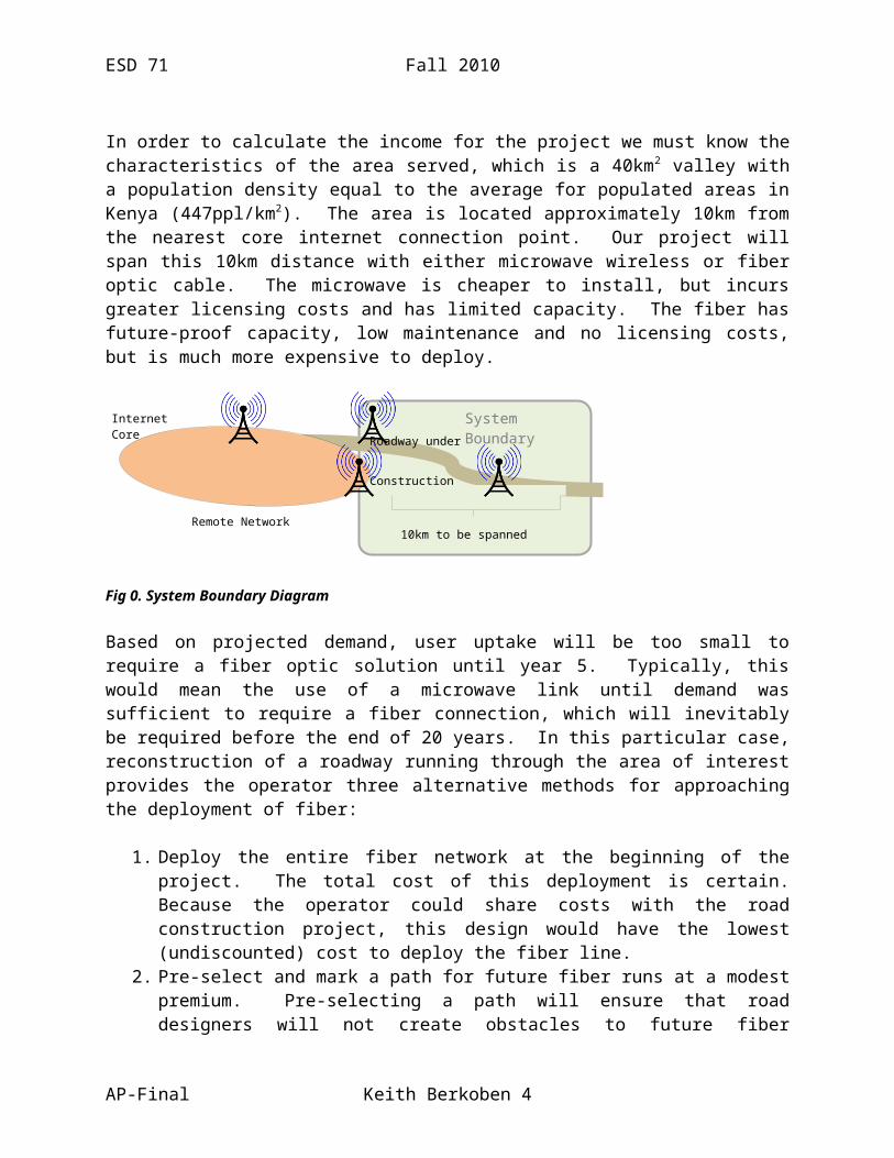
In order to calculate the income for the project we must know the characteristics of the area served, which is a 40km2 valley with a population density equal to the average for populated areas in Kenya (447ppl/km2). The area is located approximately 10km from the nearest core internet connection point. Our project will span this 10km distance with either microwave wireless or fiber optic cable. The microwave is cheaper to install, but incurs greater licensing costs and has limited capacity. The fiber has future-proof capacity, low maintenance and no licensing costs, but is much more expensive to deploy.


Internet Core

Remote Network

Roadway under Construction

System Boundary

ESD 71 Fall 2010

Fig 0. System Boundary Diagram

Based on projected demand, user uptake will be too small to require a fiber optic solution until year 5. Typically, this would mean the use of a microwave link until demand was sufficient to require a fiber connection, which will inevitably be required before the end of 20 years. In this particular case, reconstruction of a roadway running through the area of interest provides the operator three alternative methods for approaching the deployment of fiber:

1. Deploy the entire fiber network at the beginning of the project. The total cost of this deployment is certain. Because the operator could share costs with the road construction project, this design would have the lowest (undiscounted) cost to deploy the fiber line.

2. Pre-select and mark a path for future fiber runs at a modest premium. Pre-selecting a path will ensure that road designers will not create obstacles to future fiber deployment. This approach will fix the cost of a future fiber installation at a total cost below the average for buried fiber.

3. Do no preparation for fiber deployment until the fiber is actually needed. In this approach, the operator will gamble on the future deployment cost of the fiber line.

In order to determine the most desirable decision, we will simulate the growth of demand over the next 20 years in order to determine the most desirable approach. The specifics of each design alternative will be outlined more thoroughly in the Design Concepts and Option Prices section.

Principal Uncertainties – Data and Models

User Demand

The key uncertainty in this problem is user demand. In this case it is equally as difficult to determine the expected initial demand as it is to predict its future evolution. Two sources, the ITU and CCK both quote numbers and display trends for Kenyan internet subscriptions, but the two sources disagree significantly in both the total number of subscriptions and their rate of growth. The ITU suggests a .94% total subscription rate, while CCK suggests 5.1%. Similarly, the growth rate calculated from ITU data was roughly 21% (r2=.8945) compared to the CCK’s last stated value of nearly 56%2,3. The large discrepancy in the two sources suggests a potential difference in measurement methods or categorization, but without any way to explicitly disambiguate the data we are forced to treat both as potentially correct and create a distribution for which both values are potentially reasonable.

For absolute number of subscribers, we maintain the assumption that ITU and CCK data represent low and high estimates of total demand. The model assumes that any value between the ITU and CCK data is equally likely, 3.0% being the average value. We represent this uncertainty by the function:


ESD 71 Fall 2010

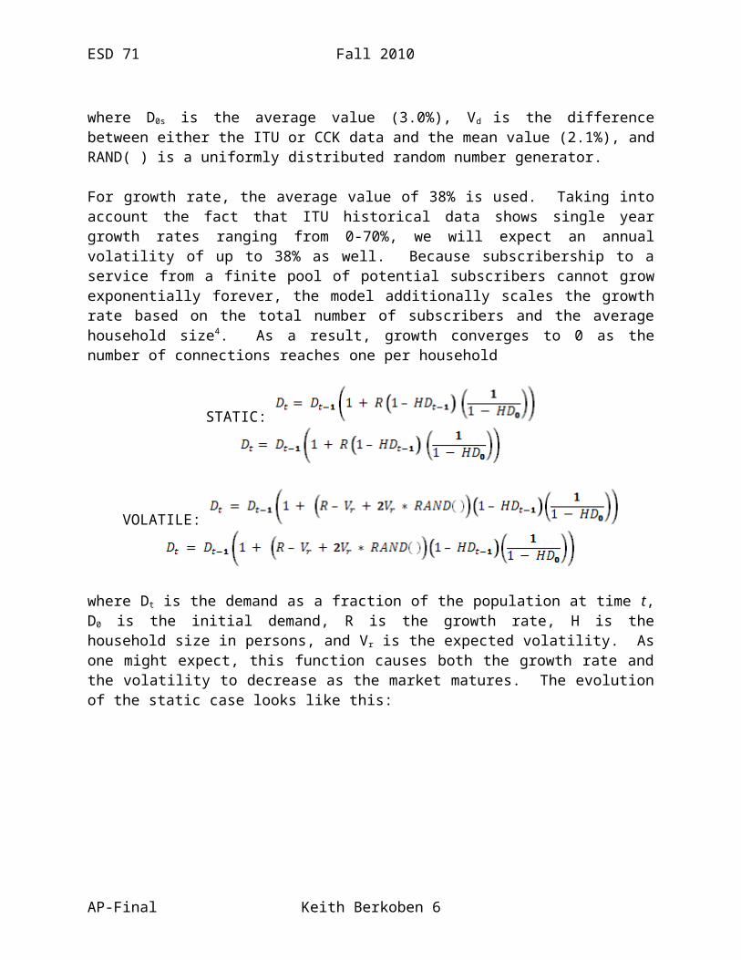
where D0s is the average value (3.0%), Vd is the difference between either the ITU or CCK data and the mean value (2.1%), and RAND( ) is a uniformly distributed random number generator.

For growth rate, the average value of 38% is used. Taking into account the fact that ITU historical data shows single year growth rates ranging from 0-70%, we will expect an annual volatility of up to 38% as well. Because subscribership to a service from a finite pool of potential subscribers cannot grow exponentially forever, the model additionally scales the growth rate based on the total number of subscribers and the average household size4. As a result, growth converges to 0 as the number of connections reaches one per household

STATIC:

VOLATILE:

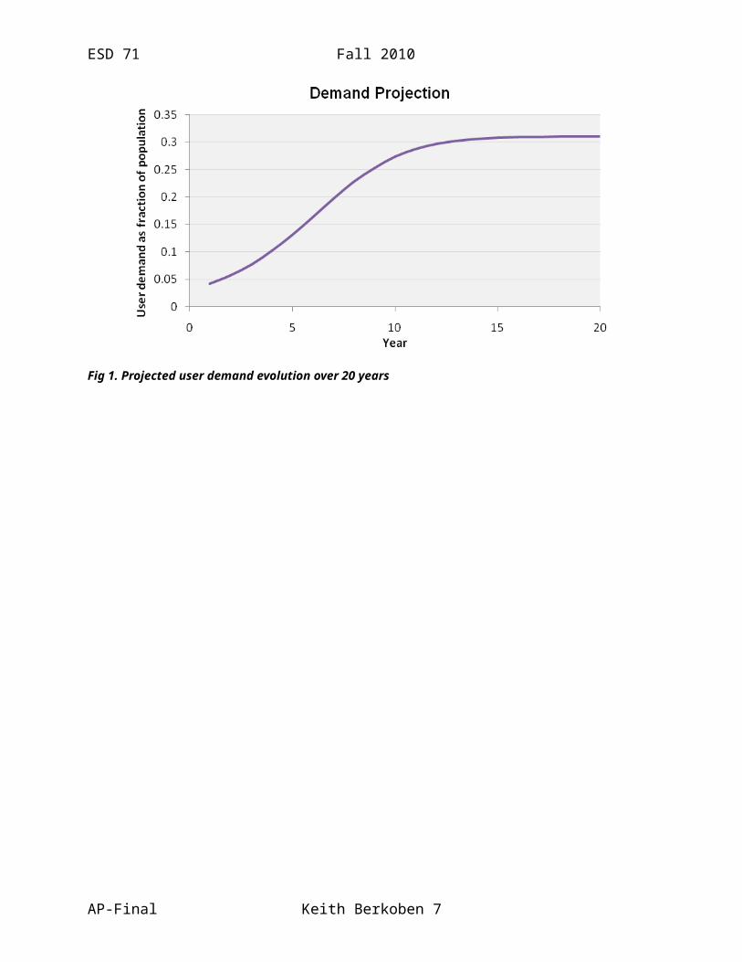
where Dt is the demand as a fraction of the population at time t, D0 is the initial demand, R is the growth rate, H is the household size in persons, and Vr is the expected volatility. As one might expect, this function causes both the growth rate and the volatility to decrease as the market matures. The evolution of the static case looks like this:

Fig 1. Projected user demand evolution over 20 years


ESD 71 Fall 2010

Combining the uncertainty in initial value and demand growth, yields the following PDF for the demand in year 20:

Fig 2. Probability distribution of user demand as a fraction of total population at the end of 20 years. The highly skewed output illustrates the fact that the market will almost surely saturate over the time interval.

And the average demand over the time interval

Fig 3. Probability distribution of average 20 Year demand as a fraction of total population. While the market is very likey to saturate by the end of 20 years, there is a wide distribution of average demand over the 20-year period.

Cost to deploy fiber

According to a recent FCC study5, deploying buried fiber can cost anywhere between $15K and $95K/km. An email 2007 email from a KDN employee on a public listserve6 estimating a


ESD 71 Fall 2010

Nairobi-Mombasa fiber link at $30k/km confirms that the FCC range is reasonable. Based on the information regarding the Nairobi-Mombasa link (buried fiber along a major roadway), we will assume that our link will be better-than-average cost to deploy in the uncertain case, yielding the range $15-55K/km. Being a shorter link, it is reasonable to expect that the average value ($35k/km) would be larger than the 435km link. The model represents this uncertainty with the function:

C = 40,000 * RAND ( ) + 15,000

The prices for the design alternative cases will be discussed in the design alternatives section.

Other Key Values

Backhaul Prices

As a second-mile provider, we are paid a price per Mbps to provide capacity to our customer. In this case we happen to be a monopoly provider, so we can rely on the original negotiated price.

Because we only provide domestic backhaul, we are not sensitive to the prevailing prices for international connectivity7. As long as international prices remain stable enough that price changes are absorbed by last-mile providers, we don’t expect to see any effects of its volatility. In the event that international prices rise so sharply that the last-mile operator could not make a profit, we might be required to make concessions or expect to see decreased growth due to price increases to the end-user, but the steady growth of international capacity suggests that this situation is very unlikely to occur. On the reverse side, a sharp decline in prices to the end-user might change our growth function, however the last-mile provider is also a monopolist at the outset and unlikely to change prices significantly without a competitive entry into the market.

Reliable data on wholesale domestic backhaul pricing is remarkably difficult to come by, however the previously discussed message from a KDN employee that 1Million Ksh/mo buys roughly 10Mbps of connectivity on a 435km fiber line. We also know from Kenyan news that KDN has decreased prices by roughly 40% on domestic links since 2007 when the message was posted. Converting to dollars and scaling to 10km we arrive at a price of about $138/Mbps/yr for our deployment.

Bandwidth demand per user

In order to convert user demand to bandwidth demand, we use a value quoted in the FCC study of .16Mbps/user.

Discount Rate

In the Kenyan technology market there are many growth opportunities. As shown in the ITU data, which was the more conservative of the two sources on market growth, there was a growth rate of 21%. A technology provider should expect a project to capture this growth minus erosion by price competition with competitors. As expected, fitting an exponential trend to the pretax profits of KDN over the last four years8 yields a growth rate of 15%. We will use 15% as our


ESD 71 Fall 2010

discount rate.

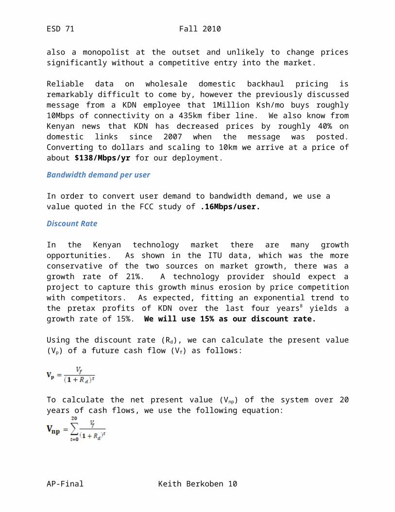
Using the discount rate (Rd), we can calculate the present value (Vp) of a future cash flow (Vf) as follows:

To calculate the net present value (Vnp) of the system over 20 years of cash flows, we use the fol-lowing equation:

Design Concepts and Design alternative Prices

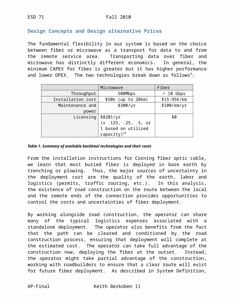
The fundamental flexibility in our system is based on the choice between fiber or microwave as a transport for data to and from the remote service area. Transporting data over fiber and microwave has distinctly different economics. In general, the minimum CAPEX for fiber is greater but it has higher performance and lower OPEX. The two technologies break down as follows9:

Microwave FiberThroughput 500Mbps > 10 Gbps

Installation cost $50k (up to 20km) $15-95k/kmMaintenance and power $300/yr $100/km/yr

Licensing $8201/yr (x .125, .25, .5, or 1 based on utilized capacity)10

$0

Table 1. Summary of available backhaul technologies and their costs

From the installation instructions for Corning fiber optic cable, we learn that most buried fiber is deployed in bare earth by trenching or plowing. Thus, the major sources of uncertainty in the deployment cost are the quality of the earth, labor and logistics (permits, traffic routing, etc.). In this analysis, the existence of road construction on the route between the local and the remote ends of the connection provides opportunities to control the costs and uncertainties of fiber deployment.

By working alongside road construction, the operator can share many of the typical logistics expenses associated with a standalone deployment. The operator also benefits from the fact that the path can be cleared and conditioned by the road construction process, ensuring that deployment will complete at the estimated cost. The operator can take full advantage of the construction now, deploying the fiber at the outset. Instead, the operator might take partial advantage of the construction, working with roadbuilders to ensure that a clear route will exist for future fiber deployment. As described in System Definition, this leads to the development of three separate design alternatives, DA1-3, as described below:


ESD 71 Fall 2010

- DA1, Full-Deploy Fiber: In this design, the operator deploys the entire fiber network at the beginning of the project. The fiber build will cost $25K/km and the microwave system will not be deployed.

- DA2, Partial-Deploy Fiber (flexible): In this design, the operator pre-selects and marks a path for future fiber deployment at the beginning of the project. The selection and marking project process will cost $1K/km. In order to service the initial demand, this design requires the use of a microwave wireless system, costing $50K to deploy. The operator will deploy fiber later, as required, with a certain cost of $30K/km.

- DA3, No Fiber Prep (flexible): In this design, the operator only deploys the Microwave system at the outset at a cost of $50K. He does not invest in preparing for a future fiber deployment. In this design, the operator will also deploy fiber later, as required, but with uncertain cost between $15K and $55K.

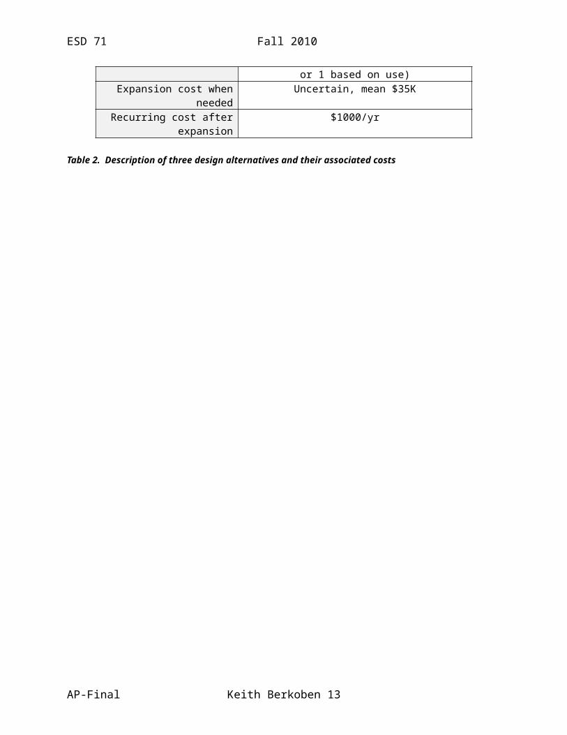
In addition to the capital costs above, design alternatives have different recurring costs in the first phase as outlined below. All designs are identical once fiber has been fully deployed. The design alternatives can be summarized as follows:

DA1: Fiber Full-Deploy Cost in year 1 $250k

Recurring cost $1000/yrDA2: Fiber Partial-Deploy (flexible)

Cost in year 1 $10k + MicrowaveRecurring cost $0/yr + Microwave

Expansion cost when needed $300kRecurring cost after expansion $1000/yr

DA3: No Fiber Prep (flexible)Cost in year 1 $50k

Recurring cost $300/yr + $8201/yr (x .125, .25, .5, or 1 based on use)Expansion cost when needed Uncertain, mean $35K

Recurring cost after expansion $1000/yr

Table 2. Description of three design alternatives and their associated costs


ESD 71 Fall 2010

Decision Rules

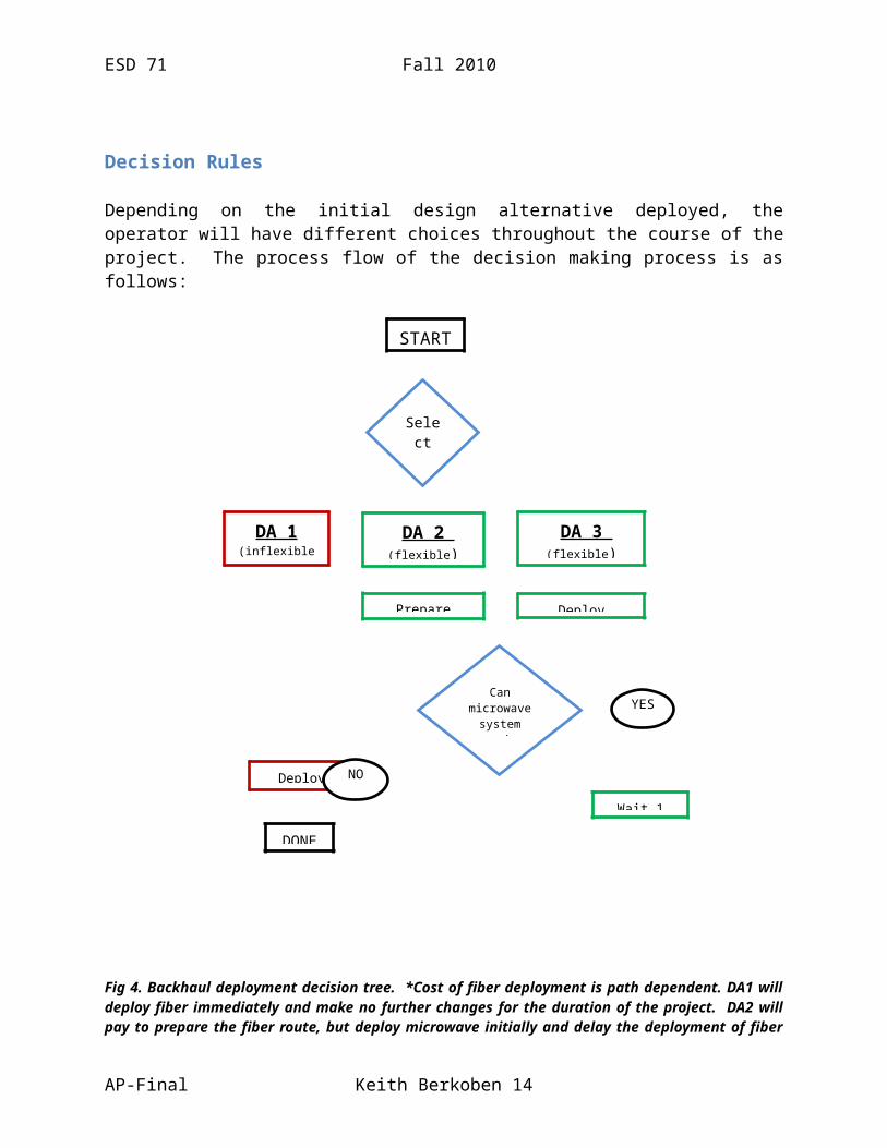
Depending on the initial design alternative deployed, the operator will have different choices throughout the course of the project. The process flow of the decision making process is as follows:

Fig 4. Backhaul deployment decision tree. *Cost of fiber deployment is path dependent. DA1 will deploy fiber immediately and make no further changes for the duration of the project. DA2 will pay to prepare the fiber route, but deploy microwave initially and delay the deployment of fiber until it is needed. DA3 will initially deploy microwave wireless and install fiber from scratch when it is needed.

For DA2-3 the operator will need to decide when to upgrade his capacity. To do this he will estimate from history data when the demand will exceed current capacity. In order to enforce a realistic decision, the model assumes that a decision-maker will make the decision to have additional capacity at time t using the demand at time t-1, receiving this capacity at time t+1. Because our model’s variation is random about a mean growth rate, we know a-priori that the


START

DA 1 (inflexible)

Deploy Fiber*

DONE

Can microwave

system service demand?

Select Design

DA 2 (flexible)

DA 3 (flexible)

Wait 1 Year

NO

Prepare fiber path Deploy Microwave

YES

ESD 71 Fall 2010

best estimate of the growth rate at any given time will be the function:

as described in Principal Uncertainties. The operator can interpret the output of the demand projection in different ways to make a decision. For example, he might decide to expand when the mean projected demand is greater than the capacity of the microwave system. Instead, he might account for volatility and expand only when the projection exceeds the microwave capacity by a capacity by a certain amount. To illustrate how this works, let’s take a numerical example:

Imagine it is currently year 4. System demand at the end of year 3 was 420Mbps and the mean projected growth rate at the current user demand is 10%. Based on this growth rate the demand can be expected to reach roughly 508Mbps at the end of year 5 (for simplicity we are neglecting the effect of increasing demand on the growth rate). A decision rule of expanding when mean projected demand exceeds microwave capacity (500Mbps) would cause the operator to initiate the fiber upgrade in year 4. If the decision rule was to expand when projected demand was 110% of capacity (550Mbps), the operator would wait at least an additional year before deploying the fiber line.

This analysis develops the decision rule in two stages. First, all the design alternatives are tested using a decision rule that expands the system when the projected demand based on the mean growth rate exceeds the capacity of the microwave system in period t+1 by any amount. The most promising selection from the first stage analysis will then be subjected to sensitivity analysis using different decision thresholds to find the most profitable rule.

The Model

Model Design

In order to test the outcomes of different decisions, we employ a simulation model running in Excel. We believe this is the ideal choice because of the multiple uncertainties and variable growth rates inherent to the problem. For each design alternative the model calculates the NPV for the projected demand and then simulates ENPV over a period of 20 years. The image on the following page shows a typical page for one of the design alternatives. In the run shown, demand increased more slowly than projected and the design alternative to build fiber capacity was exercised in year 7, yielding a 20-year NPV of $166,979.


ESD 71 Fall 2010

Fig 5. Sample page from model simulation showing a single run of a 20-year simulation

Precision Checking

Because the simulation generates expected values iteratively, it is important to ensure the simulation ran enough times to yield consistent results. Starting with a base run of 2000 iterations, the number of iterations was increased until 10 successive runs of the simulation with a set number of iterations resulted in ENPV values within 1% of their collective mean for each design alternative. As seen in the chart below, sufficient precision was achieved at 25,000 iterations.

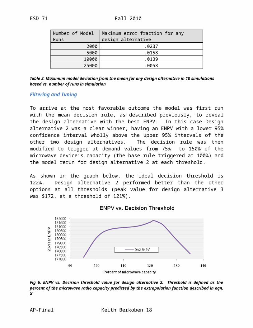
Number of Model Runs Maximum error fraction for any design alternative2000 .02375000 .0158

10000 .013925000 .0058

Table 3. Maximum model deviation from the mean for any design alternative in 10 simulations based vs. number of runs in simulation

Filtering and Tuning

To arrive at the most favorable outcome the model was first run with the mean decision rule, as described previously, to reveal the design alternative with the best ENPV. In this case Design alternative 2 was a clear winner, having an ENPV with a lower 95% confidence interval wholly above the upper 95% intervals of the other two design alternatives. The decision rule was then modified to trigger at demand values from 75% to 150% of the microwave device’s capacity (the base rule triggered at 100%) and the model rerun for design alternative 2 at each threshold.


ESD 71 Fall 2010

As shown in the graph below, the ideal decision threshold is 122%. Design alternative 2 performed better than the other options at all thresholds (peak value for design alternative 3 was $172, at a threshold of 121%).

Fig 6. ENPV vs. Decision threshold value for design alternative 2. Threshold is defined as the percent of the microwave radio capacity predicted by the extrapolation function described in eqn. X

At this threshold the system tends to slightly underservice demand for a single period in most cases. As a policy matter, the operator may find this undesirable for his reputation despite the higher expected value. For the purposes of our analysis, we will assume he is more concerned with expected value than reputation.

The application of the 122% rule improves the outcome of the other flexible design alternative (DA3) such that its ENPV is now superior in expectation to the inflexible one (DA1), despite still being inferior to DA2.

Results and Analysis

Mental Model

In order to contextualize the results of any model, a modeler must be able to stand in the shoes of the system operator. In our case, we are modeling for a network operator. This network operator has significant capital invested in physical plant and operates with small profit margins on invested capital. He requires large positive cash flows in order to amortize his investments in physical plant. Such a network operator is likely to be most interested in stable investments, especially those that can guarantee positive cash flow. Since this operator dedicates so much of his income to capital equipment, he is likely to be much more receptive to projects that can generate cash with a smaller capital burden. The operator is less likely to be receptive to high return projects with a big downside, even if they are superior in expectation. The following decision metrics will be discussed through the lens of the network operator


ESD 71 Fall 2010

Output Metrics

ENPV

The three design alternatives have ENPV values as listed in the table below:

Design alternative # -95% ENPV +95% Standard DeviationDesign alternative 1 169,627 170,823 172,020 96,545Design alternative 2 (flex) 180,177 181,023 181,869 68,228Design alternative 3 (flex) 171,135 172,102 173,069 78,032

Table 4. ENPV values for three design alternatives over20 years, including 95% intervals and standard deviation for ENPV.

Design alternative 2 is clearly the best design alternative by the ENPV metric, having no overlap in confidence intervals with either of the other two design alternatives. Unless other features of this design alternative are particularly undesirable, it is likely to be the preferred one. Having the lowest standard deviation, design alternative 2 is also likely to be the most consistent in its return – a desirable feature for the operator.

VARG Curve

The VARG curve below shows that no solution is stochastically dominant, however design alternative 2 has the desirable feature of being more profitable in the low-demand cases. Both flexible design alternatives (2, 3) are desirable in this regard, having a less than .2% probability of a negative outcome, compared with the inflexible design alternative’s 1.2% probability.

Fig 7. VARG curve for 20-year simulation of three design alternatives. Alternative 2 shows the best performance for low demand scenarios and the most robust response to user demand.


ESD 71 Fall 2010

Again, we are led to prefer Design alternative 2 over all others.

Benefit-Cost Ratio

By summing the present values of all profits and all costs over the period of interest, the benefit:cost (B/C) ratio provides a metric of how efficiently our cash flow is generating profit. This metric is particularly useful in our case because each design alternative is servicing almost exactly the same total demand and using similar technologies. This leaves deployment strategy as the independent variable affecting the outcome. The model simulates the Expected B/C ratios for each design alternative, resulting in the following values:

Design alternative # B/C ratioDesign alternative 1 1.664

Design alternative 2 (flex) 1.755Design alternative 3 (flex) 1.752

Table 5. Benefit-cost ratio for three design alternatives.

In this case Design alternatives 2 and 3 are superior, and the same within the margin of error.

ENPV/CAPEX

As the operator is sensitive to the amount of capital plant he must carry to generate profits, ENPV/CAPEX is an important metric. Depending on how the operator finances capital expenses he may or may not be sensitive to when these expenses occur in the project timeline. As a result we calculate two values below; ENPV/CAPEX0 defined as the ratio of earnings to initial capital outlay (the traditional method), and ENPV/CAPEXPV defined as the ratio of earnings to the present value of all capital equipment purchases over the life of the project.

Design alternative # ENPV/CAPEX0 ENPV/CAPEXPV

Design alternative 1 0.678 0.678Design alternative 2 (flex) 3.017 1.006Design alternative 3 (flex) 3.442 1.033

Table 6. Two formulations of ENPV/CAPEX. ENPV/CAPEX0 describes the expected net present value in relation to capital expenditure at t0. ENPV/CAPEXPV describes expected net present value in relation to the present value of all capital expenditure over the 20-year life of the project.

Design alternative 3 is superior on both of the metrics above, suggesting that it is the least capital-intensive design alternative.

Value of Flexibility

While it is clear from the analysis above that a flexible design will yield superior results, it is of interest to know exactly how much we would be willing to spend, in the theoretical case, to have flexibility. To do this we calculate the cost of the flexibility and add it to the difference in ENPV


ESD 71 Fall 2010

between the flexible and inflexible case. For Design alternative 2, the cost of the flexibility is the present value of the additional capital costs and license fees required to build in flexibility. Comparing Design alternative 1 and Design alternative 2 we find the following (undiscounted):

Category Design alternative 1

Design alternative 2

Difference

Direct design alternative Cost 0 10,000 10,000Cost of fiber install 250,000 300,000 50,000

Cost of microwave radio 0 50,000 50,000Cost of radio License 0 Up to 8,201/yr Up to 8201/yr

Table 7. Undiscounted costs for adding flexibility compared to the inflexible alternative (left col). Cost of flexibility is defined here as the additional CAPEX and license fees required to deploy flexibility over project life.

In simulation, these costs have a present value of $101,097. To determine the “raw” value of flexibility, We add the present value of the costs to the ENPV of design alternative 2, then subtract the ENPV of design alternative 1. This yields a raw value of flexibility that is roughly $120,300. In expectation, we would still be willing to implement design alternative 2 if it were to cost any amount less than this value to add the flexibility.

Sensitivity Analysis

While the above decision is reasonably clear based on the given input values, the results might change significantly if the inputs were to change. Below we graph ENPV vs input for each design while varying bandwidth price, growth rate, and initial subscriber fraction by up to 20%.

Design alternative 1 is the most sensitive to changes in all input variables, while Design alternative 3 is generally least sensitive. It is also evident that as each of the inputs tend toward higher cash flow in earlier periods design alternative 1 (building fiber at t0) begins to dominate. We would expect this to be the case as design alternative 1 has the highest initial CAPEX and the lowest recurring cost for capacity. For all variables, input values of 115% or less of the original value result in design alternative 2 showing the best result.


ESD 71 Fall 2010

Fig 8. 20-year ENPV response to changes in bandwidth price. X-unit is the fraction of predicted starting price.

Fig 9. 20-year ENPV response to changes in starting growth rate. X-unit is the fraction of predicted starting mean growth rate.

Fig 10. 20-year ENPV response to changes in initial number of subscribers. X-unit is the fraction of predicted starting mean user demand

Looking at design alternatives 1 and 2 only, we can also compare relative sensitivity to different inputs. As shown below, the outcomes for both are most sensitive to Bandwidth prices and least sensitive to initial number of subscribers, but design alternative 1 exhibits a greater potential for loss in the case of underestimates than design alternative 2


ESD 71 Fall 2010

Fig 11. Comparative sensitivity of design alternative 1 to variations in input variable values. Each value is varied by 20% above and below its projected start value.

Fig 12. Comparative sensitivity of design alternative 2 to variations in input variable values. Each value is varied by 20% above and below its projected start value.

Summary

This case clearly exhibits the value of flexibility in excess of its cost. By nearly all metrics, the flexible design alternative (2) is superior to the inflexible one. While design alternative 2 is not the most capital efficient option, it provides a greater expected value, more limited downside, lower volatility and greater robustness to error in the input values that would be desirable to the risk adverse client. Based on this analysis we would recommend that the client make the investment to prepare the fiber path and deploy fiber on demand (design alternative 2).

Reflection

Applications for Flexibility

Fundamentally, the value of flexible design is realized through the management of uncertainty, but all uncertainty is not created equal. Some sorts of deviations from projected circumstances, such as the price of a commodity, have an incremental effect on the performance of an inflexible system while others, such as a change in what product a plant manufactures, are disruptive. Systems where a deviation from the projected future has a disruptive effect on the “optimal” design often have potentially greater opportunities for flexibility to add value. Take, for example, a factory designed to produce a particular consumer product requiring heavy


ESD 71 Fall 2010

equipment, such as a model of car. If the expected model is prematurely discontinued, there is a large opportunity for loss unless the heavy equipment is reusable to produce another model. Not surprisingly, many auto manufacturers design multiple models on the same platform, increasing the interchangeability of parts and manufacturing facilities. Following from this example, projects with large capital costs, long build times and long lifetimes are better candidates for flexible design. Systems that are inherently modular with short hardware lifetimes, such as clustered computers, are less likely to benefit from flexible design methods. I think that flexible design will be very important to consider in relation to our energy dependence in the next 50 years. Given the growing focus on climate change, it is likely that energy policy will limit CO2

emissions during the lifetime of any combustion-based power plant built today. We don’t know if or when the legislation will come, or the extent of the limits. For plant owners, the flexibility to add CO2 controls or switch fuel types could prevent a complete plant overhaul in the event that regulations are enacted. Of greater concern is the evolution of fuel prices and availability. It will be very difficult to predict commodity prices and availability far enough in advance to transition an inflexible energy infrastructure, and the consequences of being unprepared for a sudden spike in or lack of energy to fuel the economy would be catastrophic. Flexible design thinking is important here because energy producers (and also the transportation industry) will consistently gravitate toward the cheapest way of going about their business. Adoption of a flexible design approach might reveal to these actors that being prepared for the inevitable is not only the safest, but also the most economical approach.

Lessons Learned

It goes without saying that any project of this complexity is always a reminder of the value of early preparation and incremental progress. Changing my AP project and starting from scratch in the final two weeks of class was less than enjoyable. In the same vein, this project was a reminder that at least half the work is always in the last 10% of a project.

One of the most interesting things I discovered about the modeling process was how easy it is to completely upend what a model illustrates by making small, ostensibly reasonable changes in how it is constructed. It follows naturally that a modeler must develop a thorough understanding about the dynamics of the system under test and, as much as possible, validate this understanding against empirical data. For my particular area I was very surprised how often different credible data sources conflicted on basic parameters and how little documentation there was on how information was gathered or what the variables in various datasets meant. Combined with the previous observation, this observation suggests that the success of a model development is highly dependent on the participation of the client and the integrity of the information they provide. I suspect that if a modeler is not careful it is easy to end up in a situation where a model simply mirrors the client’s tautological view of the world.

Finally, I was stuck in this class how much can be learned from very simple analytical structures. The course was very effective at illustrating the face that the important factor in designing for uncertainty was not the complexity of the models but the critical thinking around how a system functions and what variables are most important.

Overall this was an enjoyable and educational experience, and I am thankful to the course staff for all their time and attention ensuring that the students were able to take something meaningful


ESD 71 Fall 2010

away from the course.

References and Endnotes


1 Provider would be required to provide 99.999% uptime, paying a penalty to the customer for any downtime. In practice, reimbursement for downtime with respect to such SLAs is a significant cost for Kenyan providers using older infrastructure. Providers have made large investments in infrastructure recently in an effort to decrease downtime costs.

2 Communications Commission of Kenya, Quarterly Sector Statistics Report Jan-Mar 2009/2010, Available at: http://www.cck.go.ke/resc/statistics/Sector_Statistics_Report_Quarter_3_2009-10.pdf [Accessed December 1, 2010].

3 International Telecommunication Union - BDT. Available at: http://www.itu.int/ITU-D/icteye/Reporting/ShowReportFrame.aspx?ReportName=/BDT/DynamicReportPublic&ReportFormat=HTML4.0&RP_int-LanguageID=1&RP_strCodeIDs=422,465,420,463&RP_intClassID=0&RP_strCountryIDs=125,244&RP_bit-Latest=False&RP_intYearFrom=2004&RP_intYearTo=2009&RP_strGroupping=rbTrendCty_rCod_rYer_c [Accessed December 1, 2010].

4 International Telecommunication Union, 2002. Network Planning. Available at: http://www.itu.int/ITU-D/tech/network-infrastructure/Nairobi-02/2-3.pdf [Accessed December 1, 2010].

5 National Broadband Plan - Working Reports & Technical Papers. Available at: http://www.broadband.gov/plan/broadband-working-reports-technical-papers.html [Accessed December 1, 2010].

6 [kictanet] ISP providers cry foul over bandwidth prices. Available at: http://lists.kictanet.or.ke/pipermail/kic-tanet/2007-March/002068.html [Accessed November 30, 2010].

7 In Africa, most internet traffic must travel off of the continent. As a result, end-user prices are very sensitive to the price of international connectivity, which is constantly in high demand.

8 Global Credit Rating Co, Kenya Data Networks, December 2009. Available at: http://www.globalratings.net/attachment_view.php?pa_id=347 [Accessed December 1, 2010].

9 Note that US prices are used here for installation and maintenance. The reasoning for such an assumption is twofold. First, most electronics and manufactured goods are sourced from outside the country and of equal or greater price than comparable goods in the US. Second, while labor may be as little as half the price as in the US, some accommodation for the corruption and inefficiency inherent to a developing market must be assumed. With these effects combined, and lacking more precise data, it is reasonable to assume the overall costs will be approximately comparable to those cited in the FCC study. Licensing costs are specific to Kenya but converted to US dollars for consistency.

10 CCK Spectrum Fees. Available at: http://www.cck.go.ke/licensing/spectrum/fees.html [Accessed December 1, 2010].

Documents

Keith Berkoben - Massachusetts Institute of Technologyardent.mit.edu/real_options/Real_opts_portfolio... · Web viewKeith Berkoben ESD71 Application Portfolio Design of a Second-Mile