KEEE313(03)

Signals and Systems

Chang-Su Kim

Course Information

Course homepage

http://mcl.korea.ac.kr

Lecturer

Chang-Su Kim

Office: Engineering Bldg, Rm 508

E-mail: changsukim@korea.ac.kr

Tutor

허육 (yukheo@mcl.korea.ac.kr)

Course Information

Objective

Study fundamentals of signals and systems

Main topic: Fourier analysis

Textbook

A. V. Oppenheim and A. S. Willsky, Signals &

Systems, 2nd edition, Prentice Hall, 1997.

Reference

M. J. Roberts, Signals and Systems, McGraw

Hill, 2003.

Course Information

Prerequisite

Advanced Engineering Mathematics

Manipulation of complex numbers

Assessment

Exercises 15 %

Midterm Exam 30 %

Final Exam 40 %

Attendance 15 %

Course Schedule

First, Chapters 1-5 of the textbook will be coveredLinear time invariant systems

Fourier analysis

Then, selected topics in Chapters 6-10 will be taught, such as

Filtering

Sampling

Modulation

Laplace Transform

Z-transform

Midterm exam: 7 APR 2016 (Thursday)

Policies and Rules

ExamsScope: all materials taught

Closed book

A single sheet of hint paper (both sizes)

AttendanceChecked sometimes

QuizzesPop up quizzes: not announced before

# of quizzes is also variant

AssignmentsNo late submission is allowed

What Are Signals and Systems?

Signals

Functions of one or more independent variables

Contain information about the behavior or

nature of some phenomenon

Systems

Respond to particular signals by producing other

signals or some desired behavior

Examples of Signals and Systems (2005)

Examples of Signals and Systems (2006)

Examples of Signals and Systems (2007)

Examples of Signals and Systems (2008)

Examples of Signals and Systems (2009)

Examples of Signals and Systems (2014)

Examples of Signals and Systems (2016)

Audio Signals

f(t)

Function of time t

Acoustic pressure

S I GN AL

Image Signals

f(x,y)

Function of spatial

coordinates (x, y)

Light intensity

Image Signals

Color images

r(x,y)

g(x,y)

b(x,y)

Video Signals

Functions of space and time

r(x,y,t)

g(x,y,t)

b(x,y,t)

Video Signals

Functions of space and time

r(x,y,t)

g(x,y,t)

b(x,y,t)

원본

안정화(warping)Rolling shutter 왜곡 제거

Systems

•Input signal: left, kick,

•punch, right, up, down,…

•Output signal: sound and graphic data

Systems

•Input image •Output image

•Image processing system

Scope of “Signals and Systems” is broad

Multimedia is just a tiny portion of signal classes

The concept of signals and systems arise in a wide variety of fields

•Input signal

•- pressure on

• accelerator

• pedal

•Output signal

•- velocity

Scope of “Signals and Systems” is broad

Multimedia is just a tiny portion of signal classes

The concept of signals and systems arise in a wide variety of fields

Input signal

- time spent

on study

Output signal

- mark on

midterm exam

Mathematical Framework

The objective is to develop a mathematical

framework

for describing signals and systems and

for analyzing them

We will deal with signals involving a single

independent variable only

𝑥(𝑡) (or 𝑥[𝑛])

For convenience, the independent variable 𝑡 (or 𝑛) is

called time, although it may not represent actual time

It can in fact represent spatial location (e.g. in image

signal)

Continuous-Time Signals 𝑥(𝑡) vs.

Discrete-Time Signals 𝑥[𝑛]

𝑥[𝑛] is defined only for integer values of the independent variable n

𝑛 = ⋯ ,−2,−1, 0, 1, 2,…

𝑥[𝑛] can be obtained from sampling of CT signals or some signals are inherently discrete

DT signalCT signal

Examples of DT Signals

Signal Energy and Power

Energy: accumulation of squared magnitudes

Power: average squared magnitudes

dttxdttxE

T

TT

22)()(lim

2 2lim [ ] [ ]

N

Nn N n

E x n x n

21lim ( )

2

T

TT

P x t dtT

21lim [ ]

2 1

N

Nn N

P x nN

Classification of signals

Category 1: Energy signal (𝐸 < and thus 𝑃 = 0)

e.g.

Category 2: Power signal (𝐸 = but 𝑃 < )

e.g.

Category 3: Remaining signals (i.e. with infinite

energy and infinite power)

e.g.

0,

0,0)(

te

ttx

t

( ) 1x t

( )x t t

Signal Energy and Power

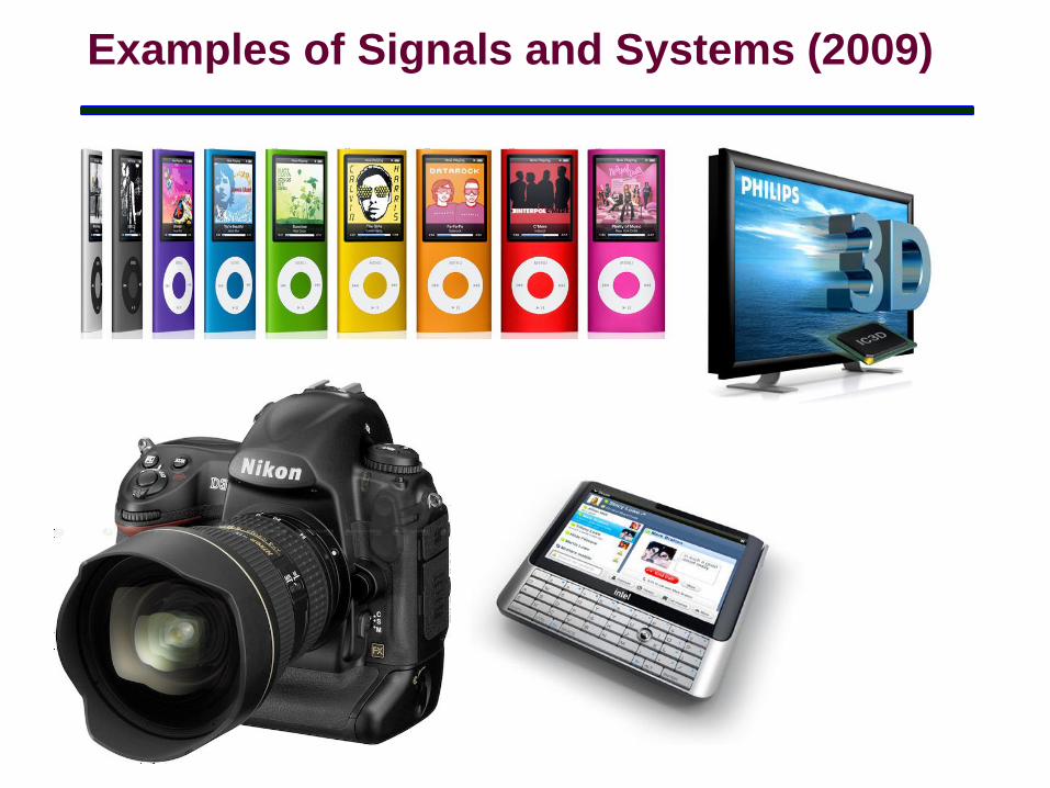
Transformations of Independent Variable

Three possible time transformations

1. Time Shift: 𝑥(𝑡 − 𝑎), 𝑥[𝑛 − 𝑎]

Shifts the signal to the right when 𝑎 > 0, while to

the left when 𝑎 < 0.

2. Time Reversal: 𝑥 −𝑡 , 𝑥[−𝑛]

Flips the signal with respect to the vertical axis.

3. Time Scale: 𝑥(𝑎𝑡), 𝑥[𝑎𝑛] for 𝑎 > 0.

Compresses the signal length when 𝑎 > 1, while

stretching it when 𝑎 < 1.

Time Reversal

Time Shift

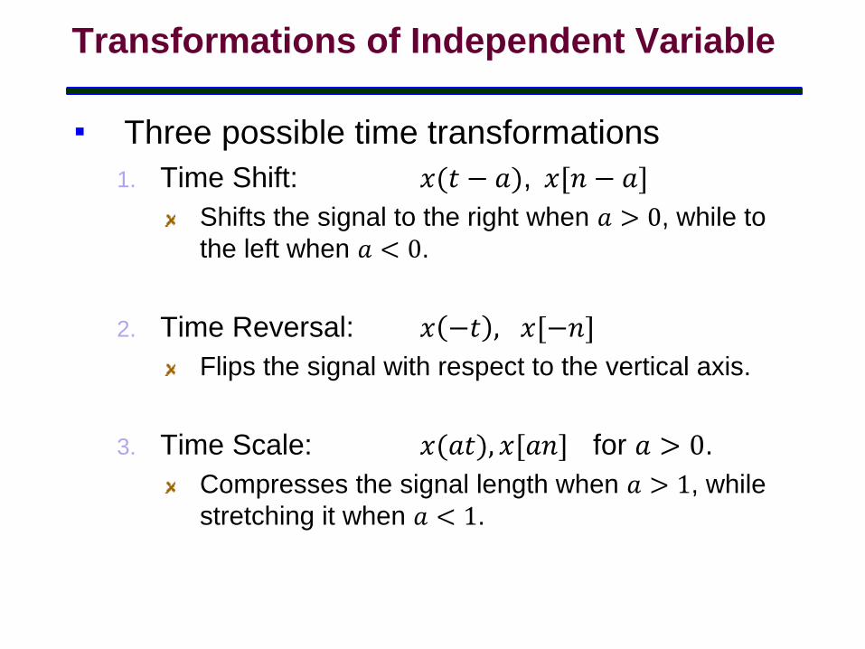
Transformations of Independent Variable

21

x(-t)

t

1

-2 -1

t

-3

x(t+1)

1

-2 -1

t

1

x(t-1)

1

-2 -1

t

x(t)

1

Time Scaling

Combinations

Transformations of Independent Variable

-1/2

t

-1

x(-2t)

1

x(-t+3)

21

t

43 65

1

-1/2

t

-1

x(2t)

1

-2 -1

t

-3

x(t/2)

-4

1

-2 -1

t

x(t)

1

Transformations of Independent Variable

Periodic Signals

𝑥(𝑡) is periodic with period 𝑇, if

𝑥(𝑡) = 𝑥(𝑡 + 𝑇) for all 𝑡

𝑥[𝑛] is periodic with period 𝑁, if

𝑥[𝑛] = 𝑥[𝑛 + 𝑁] for all 𝑛

Note that 𝑁 should be an integer

Fundamental period (𝑇0 or 𝑁0):

The smallest positive value of 𝑇 or 𝑁 for

which the above equations hold

Periodic Signals

Periodic Signals

Is this periodic?

Even and Odd Signals

𝑥[𝑛] is even, if 𝑥[−𝑛] = 𝑥[𝑛]

𝑥[𝑛] is odd, if 𝑥[−𝑛] = −𝑥[𝑛]

Any signal 𝑥[𝑛] can be divided

into even component 𝑥𝑒[𝑛] and

odd component 𝑥𝑜[𝑛]𝑥[𝑛] = 𝑥𝑒[𝑛] + 𝑥𝑂[𝑛]

𝑥𝑒[𝑛] = (𝑥[𝑛] + 𝑥[−𝑛])/2

𝑥𝑂[𝑛] = (𝑥[𝑛] − 𝑥[−𝑛])/2

Similar arguments can be made

for continuous-time signals

Even function

Odd function

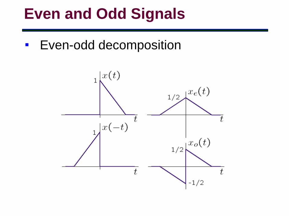
Even and Odd Signals

Even-odd decomposition

Exponential and Sinusoidal

Signals

Euler’s Equation

Euler’s formula

Complex exponential functions facilitate the manipulation of sinusoidal signals.

For example, consider the straightforward extension of differentiation formula of exponential functions to complex cases.

)(2

1sin

)(2

1cos

sincos

jj

jj

j

eej

ee

je

Periodic Signals

Periodicity conditionx(t) = x(t+T)

If T is a period of x(t), then mT is also a period, where m=1,2,3,…

Fundamental period T0

of x(t) is the smallest possible value of T.

Exercise: Find T0 for cos(0t+) and sin(0t+)

Periodicity conditionx[n] = x[n+N]

If N is a period of x[n], then mN is also a period, where m=1,2,3,…

Fundamental period N0 of x[n] is the smallest possible value of N.

CT Signal DT Signal

Sinusoidal Signals

x(t) = A cos(t+) or x[n] = A cos(n+)A is amplitude

is radian frequency (rad/s or rad/sample)

is the phase angle (rad)

Notice that although

A cos(0t+) ≠ A cos(1t+),

it may hold that

A cos[0n+] = A cos[1n+].

Do you know when?

Periodic Complex Exponential Signals

x(t) = or x[n] =

A, and are real.

Is periodic?

How about the discrete case? Is

periodic?

It is periodic when /2p is a rational number

( )j tAe ( )j nAe

( ) j tz t Ae

[ ] j nz n Ae

2

3

3

5

2

2

Ex 1) [ ]

Ex 2) [ ]

Ex 3) [ ]

j n

j n

j n

z n e

z n e

z n e

p

p

p

Review of Sinusoidal and Periodic

Complex Exponentials

CT case

These are periodic with period 2p/w.

Also,

DT case

These are periodic only if w/2p is a rational number.

Also,

( ) cos( ), sin( ) or j tx t wt wt e

[ ] cos( ), sin( ) or j nx n wn wn e

1 2

1 2

1 2 1 2

If ,

cos( ) cos( ), sin( ) sin( ) and j t j t

w w

w t w t w t w t e e

1 2

1 2

1 2 1 2

If 2 ,

cos( ) cos( ), sin( ) sin( ) and j n j n

w w k

w n w n w n w n e e

p

Real Exponential Signals

x(t) = A est or x[n] = A esn

A and s are real.

positive s negative s

General Exponential Signals

( )( )

[cos( ) sin( )]

st j jw t

t

x t Xe Ae e

Ae wt j wt

s

s

Real part of x(t) according to s ( is assumed to be 0)

Impulse and Step Functions

DT Unit Impulse Function

Unit Impulse

Shifted Unit Impulse

1, 0[ ]

0, 0

nn

n

[n]

-1-2

n

1-3 32

1

[n-k]

…-1

n

1 k

11,

[ ]0,

n kn k

n k

DT Unit Step Function

Unit Step

Shifted Unit Step

1, 0[ ]

0, 0

nu n

n

u[n]

-1-2

n

1-3 32

1

u[n-k]

…-1

n

1 k

11,[ ]

0,

n ku n k

n k

Properties of DT Unit Impulse and Step

Functions

0

0 0 0

1) [ ] [ ] [ 1]

2) [ ] [ ] [ ]

3) [ ] [ ] [0] [ ]

4) [ ] [ ] [ ] [ ]

5) [ ] [ ] [ ]

n

k k

k

n u n u n

u n k n k

x n n x n

x n n n x n n n

x n x k n k

CT Unit Step Function

Unit Step

Shifted Unit Step

1, 0( )

0, 0

tu t

t

t

1

u(t- )

t

1

u(t)

1,( )

0,

tu t

t

CT Unit Step Function

Unit step is discontinuous at t=0, so is not

differentiable

Approximated unit step

u(t) is continuous and differentiable.

0, 0

( ) , 0

1,

t

tu t t

t

t

1

u(t)

0( ) lim ( )u t u t

1, 0( )

0, otherwise

tdu t

dt

CT Unit Impulse Function

Approximated unit impulse

Unit Impulse:

0

, 0( ) lim ( )

0, 0

( ) 1 for any 0 and 0.

b

a

tt t

t

t dt a b

t

(t)

t

(t)

1, 0( )

( )

0, otherwise

tdu tt

dt

1/

CT Unit Impulse Function

Shifted Unit Impulse

t

(t-)

Properties of CT Unit Impulse and Step

Functions

0

0 0 0

( )1) ( )

2) ( ) ( ) ( )

3) ( ) ( ) (0) ( )

4) ( ) ( ) ( ) ( )

5) ( ) ( ) ( )

t

du tt

dt

u t d t d

x t t x t

x t t t x t t t

x t x t d

Comparison of DT and CT Properties

0 0

Difference becomes ( )[ ] [ ] [ 1] ( )

differentiation

Summation becomes [ ] [ ] [ ] ( ) ( ) ( )

integration

Impulse functions [ ] [ ] [0] [ ] ( ) (

sample values

tn

k k

du tn u n u n t

dt

u n k n k u t d t d

x n n x n x t t

0 0 0 0 0 0

) (0) ( )

Shifted impulse [ ] [ ] [ ] [ ] ( ) ( ) ( ) ( )

functions

Sifting Property:

Arbitrary functions as sum [ ] [ ] [ ] ( ) ( ) ( )

or integration of delta functionsk

x t

x n n n x n n n x t t t x t t t

x n x k n k x t x t d

Can you represent these functions using

step functions?

tc

x(t)

a b

1

y(t)

-1 1t

1

w(t)

-1 1t

2z(t)

-1

1t

2

-2

x[n]

…-1

n

1 N

1

y[n]

… -1

n

1 4

1

-2 32 5-3 …

Can you represent these functions using

step functions?

Basic System Properties

What is a System?

System is a black box that takes an input signal and

converts it to an output signal.

DT System: y[n] = H[x[n]]

CT System: y(t) = H(x(t))

Hx[n] y[n]

Hx(t) y(t)

Interconnection of Systems

Series (or cascade) connection: y(t) = H2( H1( x(t) ) )

e.g. a radio receiver followed by an amplifier

Parallel connection: y(t) = H2( x(t) ) + H1( x(t) )

e.g. Carrying out a team project

H1

x(t)

H1

x(t) y(t)

H2

y(t)

H2

+

Feedback connection: y(t) = H1( x(t)+H2( y(t) ) )

e.g. cruise control

Various combinations of connections are also

possible

H1

x(t) y(t)

H2

+

Interconnection of Systems

Memoryless Systems vs.

Systems with Memory

Memoryless Systems: The output y(t) at any instance t depends

only on the input value at the current time t, i.e. y(t) is a function

of x(t)

Systems with Memory: The output y(t) at any instance t depends

on the input values at past and/or future time instances as well

as the current time instance

Examples:

A resistor: 𝑦(𝑡) = 𝑅𝑥(𝑡)

A capacitor:

𝑦 𝑡 =1

𝐶න−∞

𝑡

𝑥 𝜏 𝑑𝜏

A unit delayer: 𝑦[𝑛] = 𝑥[𝑛 − 1]

An accumulator:

𝑦 𝑛 =

𝑘=−∞

𝑛

𝑥[𝑘]

Causality

Causality: A system is causal if the output at any time

instance depends only on the input values at the current

and/or past time instances.

Examples:

𝑦[𝑛] = 𝑥[𝑛] − 𝑥[𝑛 − 1]

𝑦(𝑡) = 𝑥(𝑡 + 1)

Is a memoryless system causal?

Causal property is important for real-time processing.

But in some applications, such as image processing,

data is often processed in a non-causal way.

image

processing

Applications of Lowpass Filtering

Preprocessing before machine recognition

Removal of small gaps

Applications of Lowpass Filtering

Cosmetic processing of photos

Invertibility

Invertibility: A system is invertible if distinct inputs

result in distinct outputs.

If a system is invertible, then there exists an inverse system

which converts the output of the original system to the

original input.

Examples:

)(4

1)(

)(4)(

tytw

txty

]1[][][

][][

nynynw

kxnyn

k

System𝑥(𝑡) Inverse

System

𝑤(𝑡) = 𝑥(𝑡)𝑦(𝑡)

( ) ( )

( )( )

t

y t x d

dy tw t

dt

Stability

Stability: A system is stable if a bounded input yields

a bounded output (BIBO).

In other words, if 𝑥 𝑡 < 𝑘1 then |𝑦(𝑡)| < 𝑘2.

Examples:

0

( ) ( )

t

y t x d

][100][ nxny

Linearity

A system is linear if it satisfies two properties.

Additivity: 𝑥 𝑡 = 𝑥1(𝑡) + 𝑥2(𝑡) ⇒ 𝑦(𝑡) = 𝑦1(𝑡) + 𝑦2(𝑡)

Homogeneity: 𝑥 𝑡 = 𝑐 𝑥1(𝑡) ⇒ 𝑦(𝑡) = 𝑐 𝑦1(𝑡),

for any constant 𝑐

The two properties can be combined into a single

property.

linearity:

𝑥 𝑡 = 𝑎𝑥1(𝑡) + 𝑏𝑥2(𝑡) ⇒ 𝑦(𝑡) = 𝑎𝑦1(𝑡) + 𝑏𝑦2(𝑡)

Examples

)()( 2 txty ][][ nnxny ( ) 2 ( ) 3y t x t

Time-Invariance

A system is time-invariant if a delay (or a time-shift) in

the input signal causes the same amount of delay in

the output.

𝑥 𝑡 = 𝑥1(𝑡 − 𝑡0) ⇒ 𝑦(𝑡) = 𝑦1(𝑡 − 𝑡0)

Examples:

][][ nnxny )2()( txty )(sin)( txty

Superposition in LTI Systems

For an LTI system:

Given response y(t) of the system to an input signal x(t), it is

possible to figure out response of the system to any signal

x1(t) that can be obtained by “scaling” or “time-shifting” the

input signal x(t), because

𝑥1 𝑡 = 𝑎0 𝑥 𝑡 − 𝑡0 + 𝑎1 𝑥 𝑡 − 𝑡1 + 𝑎2𝑥 𝑡 − 𝑡2 +⋯

⇒𝑦1 𝑡 = 𝑎0 𝑦 𝑡 − 𝑡0 + 𝑎1 𝑦 𝑡 − 𝑡1 + 𝑎2𝑦 𝑡 − 𝑡2 +⋯

Very useful property since it becomes possible to

solve a wider range of problems.

This property will be basis for many other techniques

that we will cover throughout the rest of the course.

Superposition in LTI Systems

Exercise: Given response y(t) of an LTI system to the input

signal x(t), find the response of that system to another input

signal x1(t) shown below.

2

x(t)

1

t1

y(t)

-1 1t

2

x1(t)

1 t

-1

3