Keck NGAO Science:Strong Gravitational Lensing

Phil Marshall and Tommaso Treu

September 2007

• Examples of strong lensing science:➔ The dark and stellar mass of elliptical galaxies out

to, and beyond z = 1➔ CDM substructure: imaging the mass➔ Super-resolving high redshift galaxies – and their

velocity fields

• “Kinematic lensing” - what a well-resolved multiply-imaged velocity field can do for you• Why can we not do this now?• Why will we need NGAO in the future?• What will we need NGAO to provide?

Outline

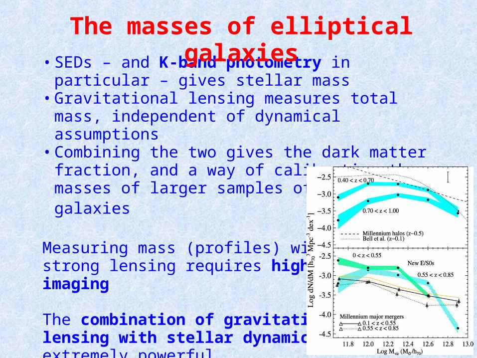
• SEDs – and K-band photometry in particular – gives stellar mass• Gravitational lensing measures total mass, independent of

dynamical assumptions• Combining the two gives the dark matter fraction, and a

way of calibrating the masses of larger samples of non-lens galaxies

Measuring mass (profiles) with strong lensing requires high resolution imaging

The combination of gravitational lensing with stellar dynamics is extremely powerful

The masses of elliptical galaxies

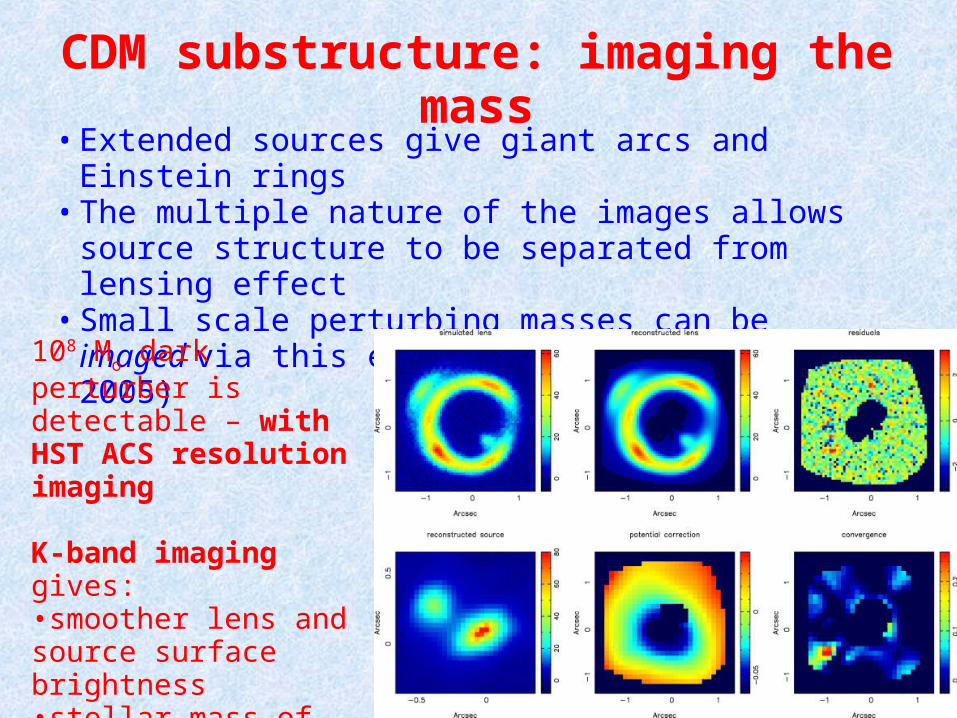
• Extended sources give giant arcs and Einstein rings• The multiple nature of the images allows source structure to

be separated from lensing effect• Small scale perturbing masses can be imaged via this effect

(eg Koopmans et al 2005)

CDM substructure: imaging the mass

108 Mo dark perturber is

detectable – with HST ACS resolution imaging

K-band imaging gives:•smoother lens and source surface brightness•stellar mass of CDM satellites

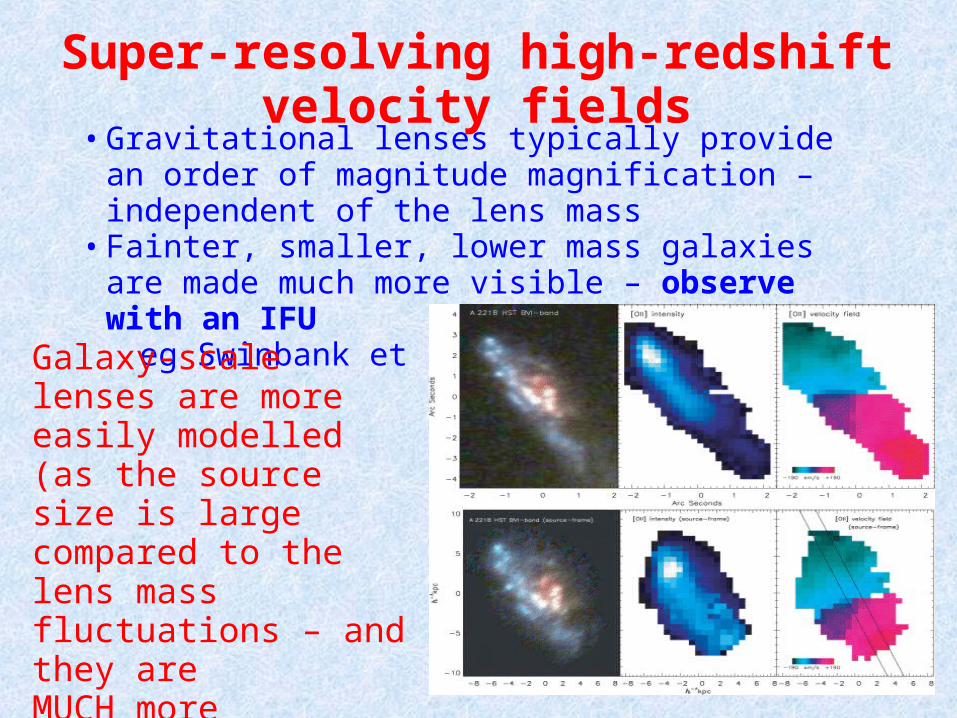
• Gravitational lenses typically provide an order of magnitude magnification – independent of the lens mass• Fainter, smaller, lower mass galaxies are made much more

visible – observe with an IFU eg Swinbank et al 2006:

Super-resolving high-redshift velocity fields

Galaxy-scale lenses are more easily modelled (as the source size is large compared to the lens mass fluctuations – and they are MUCH more numerous. Select your own cosmic telescope!

• Strong lensing science:➔ The dark and stellar mass of elliptical galaxies out

to, and beyond z = 1➔ CDM substructure: imaging the mass➔ Super-resolving high redshift galaxies – and their

velocity fields

• “Kinematic lensing” - what a well-resolved multiply-imaged velocity field can do for you• Why can we not do this now?• Why will we need NGAO in the future?• What will we need NGAO to provide?

Outline

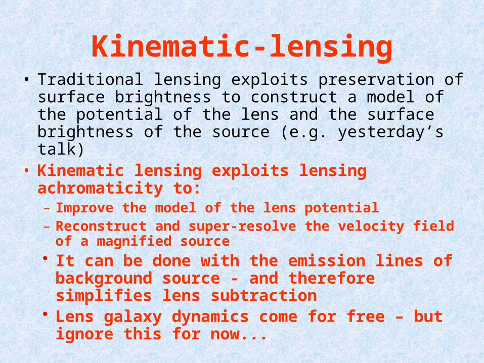
Kinematic-lensing• Traditional lensing exploits preservation of surface

brightness to construct a model of the potential of the lens and the surface brightness of the source (e.g. yesterday’s talk)

• Kinematic lensing exploits lensing achromaticity to:– Improve the model of the lens potential– Reconstruct and super-resolve the velocity field of a

magnified source• It can be done with the emission lines of

background source - and therefore simplifies lens subtraction

• Lens galaxy dynamics come for free – but ignore this for now...

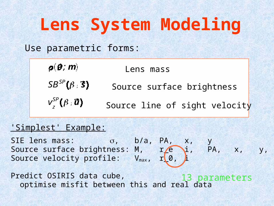
Lens System ModelingUse parametric forms:

; m

SBSP; s

vz

SP; u

Lens mass

Source surface brightness

Source line of sight velocity

SIE lens mass: , b/a, PA, x, ySource surface brightness: M, r_e i, PA, x, y,Source velocity profile: Vmax, r_0, i

Predict OSIRIS data cube, optimise misfit between this and real data

'Simplest' Example:

13 parameters

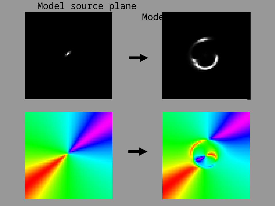
Model source plane Model image plane

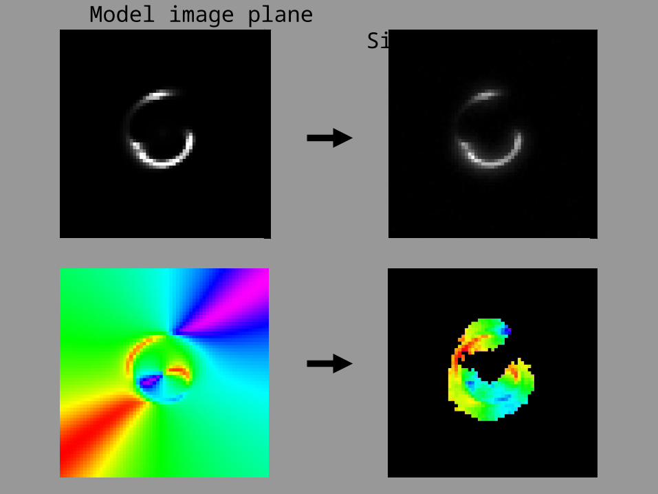
Model image plane Simulated data

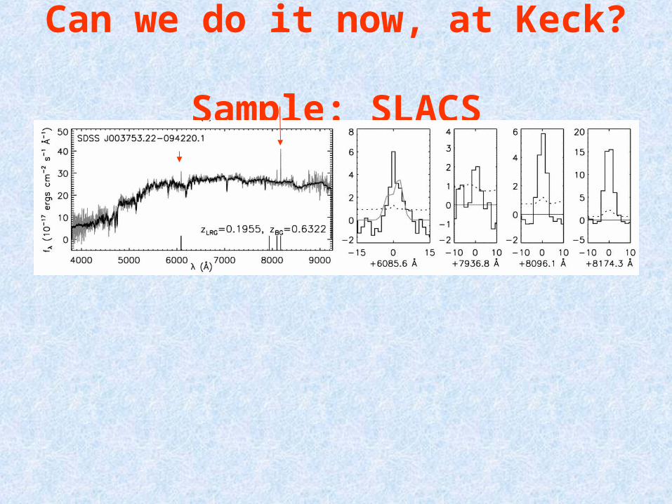
Can we do it now, at Keck? Sample: SLACS

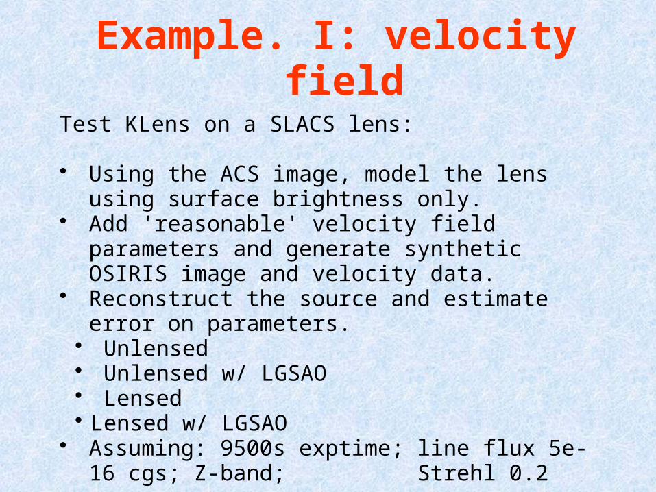
Example. I: velocity field

Test KLens on a SLACS lens:

• Using the ACS image, model the lens using surface brightness only.

• Add 'reasonable' velocity field parameters and generate synthetic OSIRIS image and velocity data.

• Reconstruct the source and estimate error on parameters.• Unlensed• Unlensed w/ LGSAO• Lensed• Lensed w/ LGSAO

• Assuming: 9500s exptime; line flux 5e-16 cgs; Z-band; Strehl 0.2

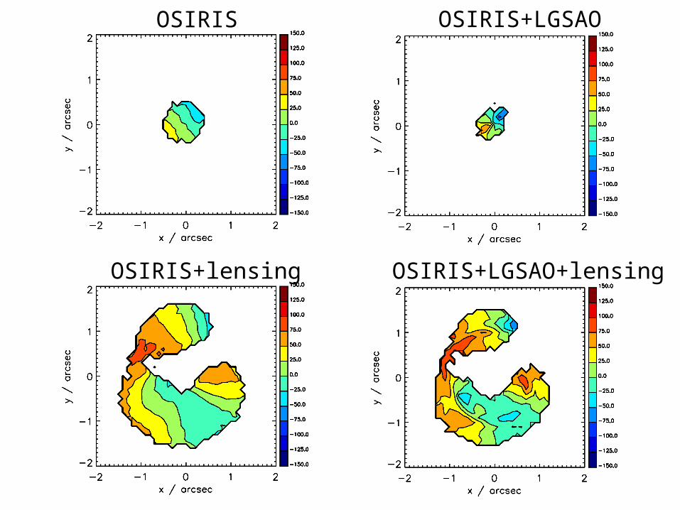
OSIRIS

OSIRIS+lensing OSIRIS+LGSAO+lensing

OSIRIS+LGSAO

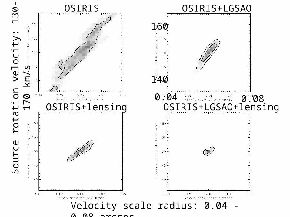
OSIRIS

OSIRIS+lensing OSIRIS+LGSAO+lensing

OSIRIS+LGSAO

Velocity scale radius: 0.04 - 0.08 arcsec

Sou

rce

rota

tion

vel

ocit

y: 1

30-1

70 k

m/s

0.04 0.08

140

160

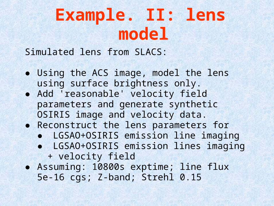
Example. II: lens model

Simulated lens from SLACS:

● Using the ACS image, model the lens using surface brightness only.

● Add 'reasonable' velocity field parameters and generate synthetic OSIRIS image and velocity data.

● Reconstruct the lens parameters for● LGSAO+OSIRIS emission line imaging● LGSAO+OSIRIS emission lines imaging + velocity

field● Assuming: 10800s exptime; line flux 5e-16 cgs; Z-band;

Strehl 0.15

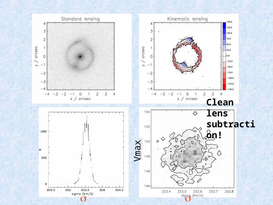
Vm

ax

Clean lens subtraction!

Does it work in practice?We don’t know yet...

• Half night allocated June 2006:• partially cloudy. 1.5 hours in three

pointings (effectively 1800s) in Z-band. No detection

• One night allocated September 2006: • completely lost to wavefront sensor

failure• With current technology is hard!• 2007: system more stable, targets

improved: Richard (Caltech) has data...

Improvements wish list:

• Higher redshift targets. In Z, OSIRIS field of view is too small, need mosaicing with loss of time: • Much better at longer wavelengths. 3.2”x6.4” or

4.8”x6.4” is larger than lens (typically <3”). Dither on targets. Larger field is more efficient

• Brighter targets:• With full SLACS (88 vs 23 last year) or SL2S we can

find even brighter emission lines• Higher Strehl ratios:

reduce exposure times and thus make it practical to collect sizeable samples.

(Beginning to sound like NGAO)

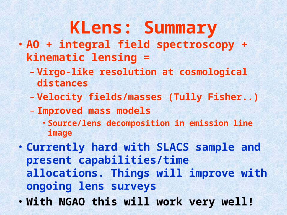
KLens: Summary• AO + integral field spectroscopy +

kinematic lensing =– Virgo-like resolution at cosmological distances– Velocity fields/masses (Tully Fisher..)– Improved mass models

• Source/lens decomposition in emission line image

• Currently hard with SLACS sample and present capabilities/time allocations. Things will improve with ongoing lens surveys

• With NGAO this will work very well!

• Strong lensing science:➔ The dark and stellar mass of elliptical galaxies out

to, and beyond z = 1➔ CDM substructure: imaging the mass➔ Super-resolving high redshift galaxies – and their

velocity fields

• “Kinematic lensing” - what a well-resolved multiply-imaged velocity field can do for you• Why can we not do this now?• Why will we need NGAO in the future?• What will we need NGAO to provide?

Outline

Current samples (eg based on SDSS) are limited to z~0.2 and contain ~100 systems

In the NGAO era, the lens sample will be an order of magnitude larger, and extend to higher redshift (z>1) – interesting subsamples can be selected and exploited

SL2S (2005-) ongoing imaging survey based on CFHTLS, finding ~100 new lenses at z~0.5-1.0

DES (2009-2014) will find a few hundred lensesPanSTARRS-1 (2008-2012) will find ~few 1000 lensesSDSS-III (2010?) ~ SLACS x 10 at higher z?LSST (2014-2024?) would find ~10,000 lensesSNAP (2019-2021?) would find ~20,000 lensesDune (2019-2021?) would find ~few 100,000 lenses

Feeder surveys

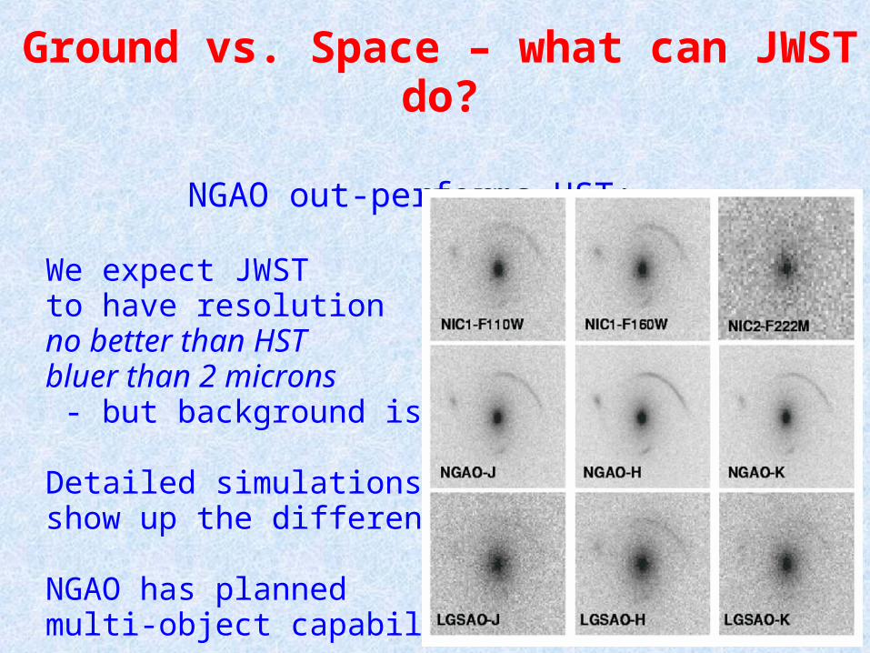
NGAO out-performs HST:

We expect JWST to have resolution no better than HST bluer than 2 microns - but background is lower

Detailed simulations will show up the differences.

NGAO has plannedmulti-object capability...

Ground vs. Space – what can JWST do?

Lenses are rare – but a Multiplex IFU:

•would speed up observation (simultaneous background monitoring)

•and allow piggy-backing on the high-z program (their targets are more common)

•and enable cluster lensing science (larger collecting area cosmic telescopes – but that's a whole other talk!)

Multiplexing over a 3' field of regard

As for the high-z galaxy program,(eg high strehl imaging, sufficient spectral resolution to measure velocities to 20km/s, low background, large fraction of sky accessible etc etc)

but with a few additions:

•> 4” IFU field of view (lenses magnify galaxies, such that ~all systems are 2-3” in diameter)

•bluer filters broaden the range of accessible redshifts, and help in SED analysis of lensed sources•z, Y bands also enable lens galaxy absorption line dynamical mass estimates at z~1

Summary: NGAO requirements

Extra slides

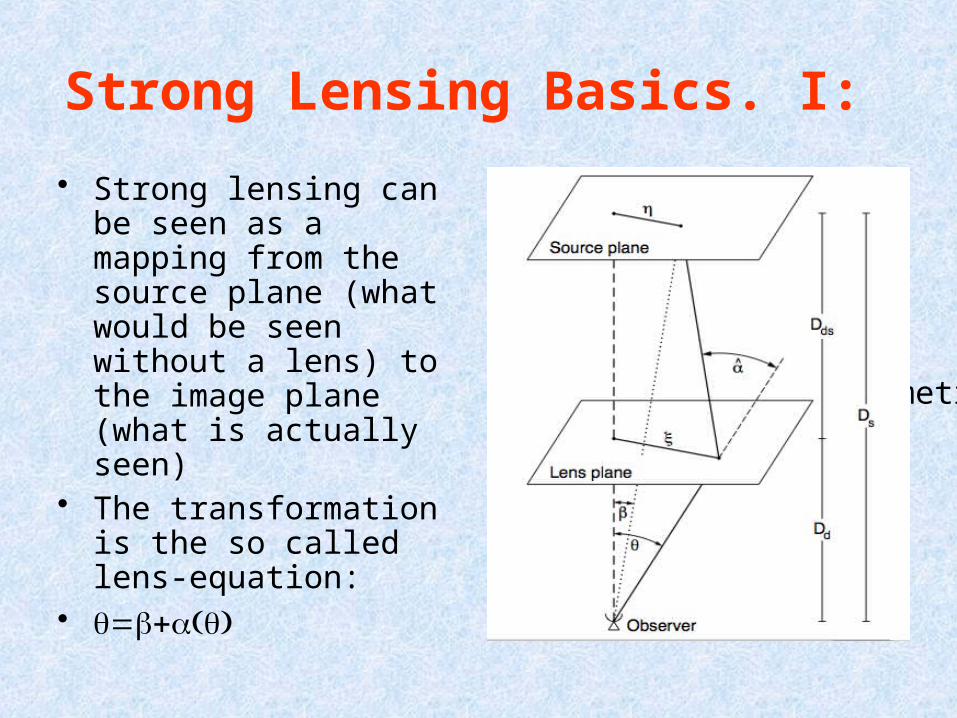
Strong Lensing Basics. I:

For azimuthal symmetry

• Strong lensing can be seen as a mapping from the source plane (what would be seen without a lens) to the image plane (what is actually seen)

• The transformation is the so called lens-equation:

•

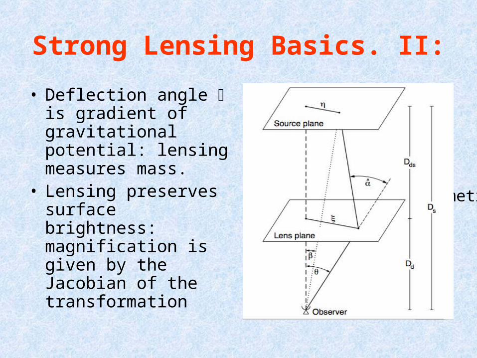
Strong Lensing Basics. II:

For azimuthal symmetry

• Deflection angle is gradient of gravitational potential: lensing measures mass.

• Lensing preserves surface brightness: magnification is given by the Jacobian of the transformation

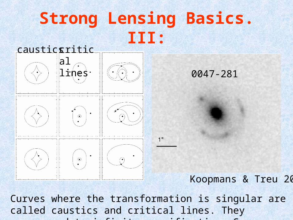
Strong Lensing Basics. III:

Curves where the transformation is singular are called caustics and critical lines. They correspond to infinite magnification. Sources get multiply-imaged when they are inside caustics. They are typically highly magnified.

Koopmans & Treu 2003

caustics critical lines

0047-281

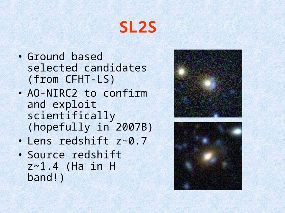
SL2S

• Ground based selected candidates (from CFHT-LS)

• AO-NIRC2 to confirm and exploit scientifically (hopefully in 2007B)

• Lens redshift z~0.7• Source redshift z~1.4 (Ha in

H band!)

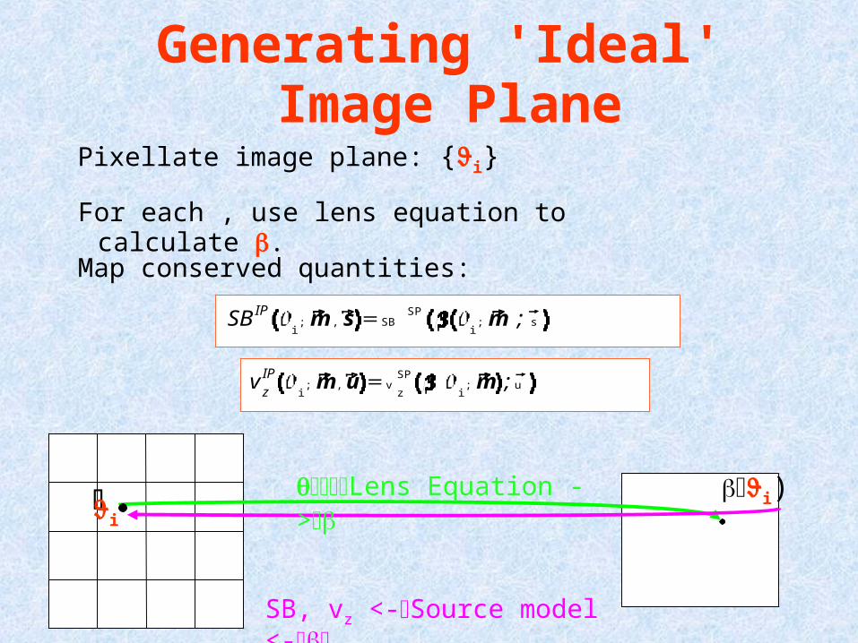
Generating 'Ideal' Image Plane

Pixellate image plane: {i}

i)Lens Equation ->

SB, vz <-Source model <-

SB IP

i; m , s SB

SP

i; m ; s

vz

IP

i; m, u v

z

SP

i; m ; u

Map conserved quantities:

For each , use lens equation to calculate .

i

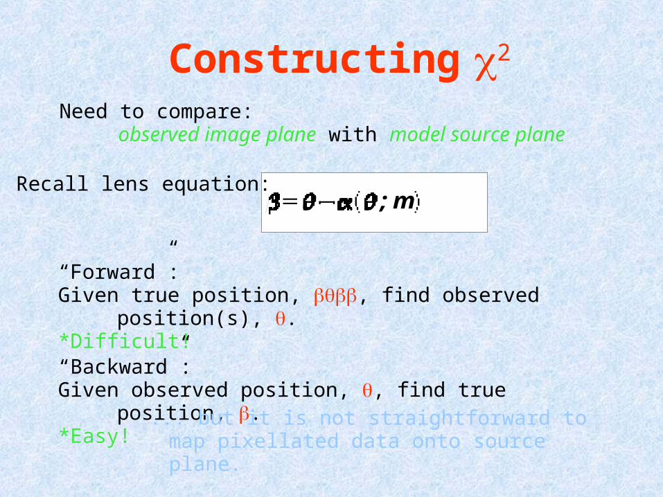
Constructing 2

Need to compare:observed image plane with model source plane

“Forward”:Given true position, , find observed position(s), .*Difficult!

“Backward”:Given observed position, , find true position, .*Easy! ... but it is not straightforward to map pixellated data

onto source plane.

; mRecall lens equation:

Creating 'Model' Image Plane

N model

i; m , s

vz

model

i; m , u

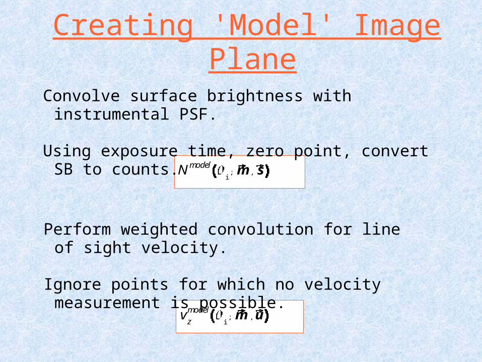
Convolve surface brightness with instrumental PSF.

Using exposure time, zero point, convert SB to counts.

Perform weighted convolution for line of sight velocity.

Ignore points for which no velocity measurement is possible.

Finding Best Parameters

2 m , s , ui

Nobs

iN

model

i; m , s

2

N

2

i

vz

obs

iv

z

model

i; m , u 2

vz

2

i

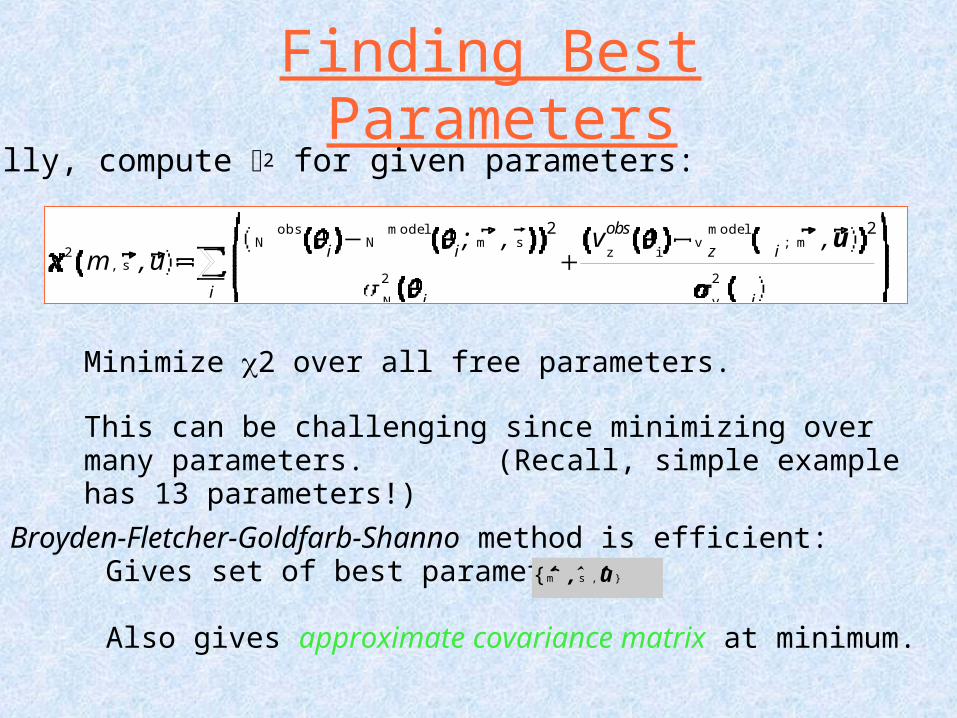
Finally, compute 2 for given parameters:

This can be challenging since minimizing over many parameters. (Recall, simple example has 13 parameters!)

Broyden-Fletcher-Goldfarb-Shanno method is efficient:Gives set of best parameters:

Also gives approximate covariance matrix at minimum.

{ m , s , u }

Minimize 2 over all free parameters.

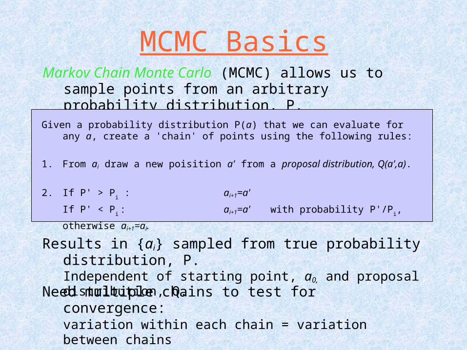
MCMC BasicsMarkov Chain Monte Carlo (MCMC) allows us to sample points

from an arbitrary probability distribution, P.

Given a probability distribution P(a) that we can evaluate for any a, create a 'chain' of points using the following rules:

1. From ai draw a new poisition a' from a proposal distribution, Q(a',a).

2. If P' > Pi : ai+1=a'

If P' < Pi : ai+1=a' with probability P'/Pi, otherwise ai+1=ai.

Results in {ai} sampled from true probability distribution, P.Independent of starting point, a0, and proposal distribution, Q.

Need multiple chains to test for convergence:variation within each chain = variation between chains

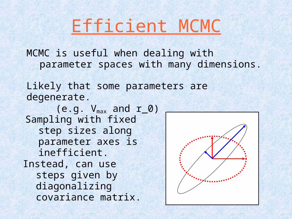
Efficient MCMC

Likely that some parameters are degenerate.(e.g. Vmax and r_0)

MCMC is useful when dealing with parameter spaces with many dimensions.

Instead, can use steps given by diagonalizing covariance matrix.

Sampling with fixed step sizes along parameter axes is inefficient.

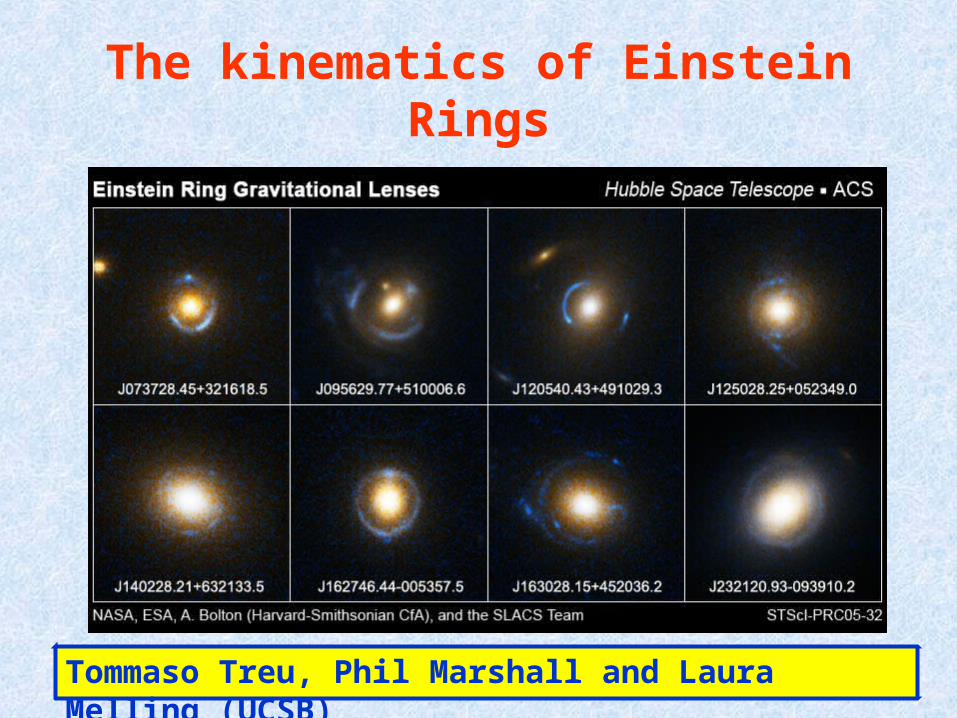
The kinematics of Einstein Rings

Tommaso Treu, Phil Marshall and Laura Melling (UCSB)

Properties of lens mapping:

• Non-linear

• Preserves surface brightness

• Independent of frequency (ACHROMATIC)

• Magnifies sources

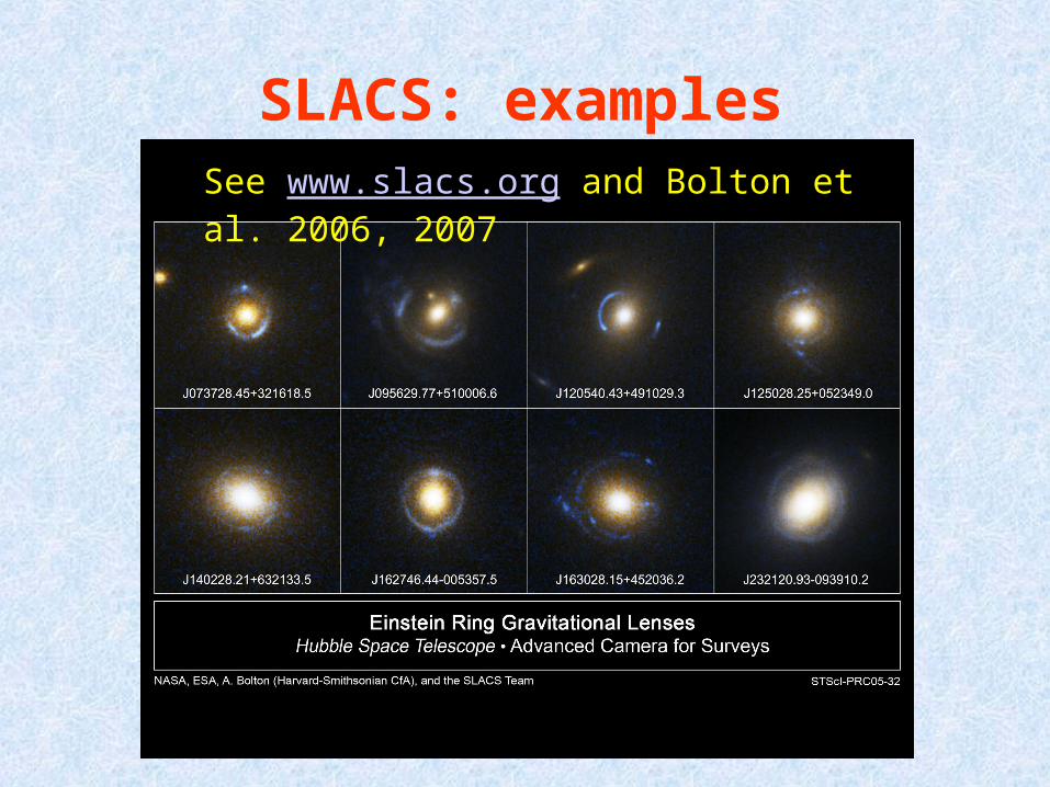
SLACS: examplesSee www.slacs.org and Bolton et al. 2006, 2007

Why do we care?

• Lensing measure masses:– Exploiting lensing achromaticity improves knowledge of

gravitational potential of deflector

• Lensing magnifies, hence “gravitational telescopes”:– The internal structure of distant galaxies can be study with a typical

factor of 10 improvement in sensitivity and spatial resolution