KDD Overview

Xintao Wu

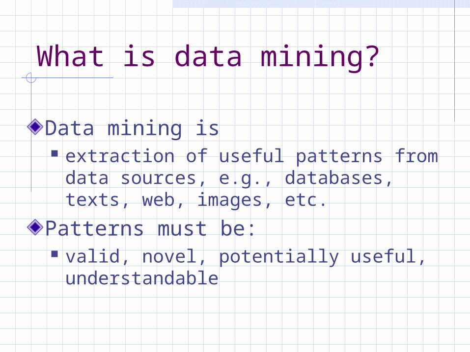
What is data mining?

Data mining is extraction of useful patterns from data

sources, e.g., databases, texts, web, images, etc.

Patterns must be: valid, novel, potentially useful,

understandable

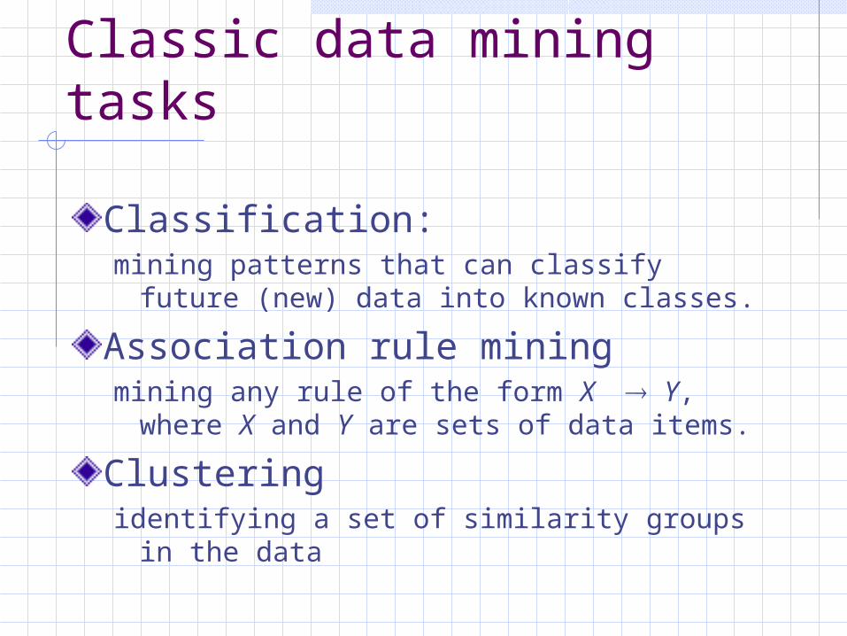
Classic data mining tasks

Classification:mining patterns that can classify future (new)

data into known classes.

Association rule miningmining any rule of the form X Y, where X

and Y are sets of data items.

Clusteringidentifying a set of similarity groups in the

data

CS583, Bing Liu, UIC 4

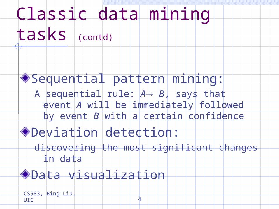
Classic data mining tasks (contd)

Sequential pattern mining:A sequential rule: A B, says that event A will

be immediately followed by event B with a certain confidence

Deviation detection: discovering the most significant changes in

data

Data visualization

Why is data mining important?

Huge amount of data How to make best use of data? Knowledge discovered from data can be used for

competitive advantage.

Many interesting things that one wants to find cannot be found using database queries, e.g.,“find people likely to buy my products”

6

Related fields

Data mining is an multi-disciplinary field:Machine learningStatisticsDatabasesInformation retrievalVisualizationNatural language processingetc.

Association Rule: Basic Concepts

Given: (1) database of transactions, (2) each transaction is a list of items (purchased by a customer in a visit)Find: all rules that correlate the presence of one set of items with that of another set of items E.g., 98% of people who purchase tires

and auto accessories also get automotive services done

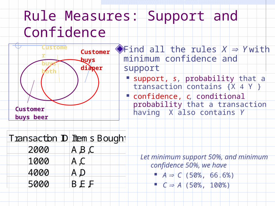
Rule Measures: Support and Confidence

Find all the rules X Y with minimum confidence and support support, s, probability that a

transaction contains {X Y } confidence, c, conditional

probability that a transaction having X also contains Y

Transaction ID Items Bought2000 A,B,C1000 A,C4000 A,D5000 B,E,F

Let minimum support 50%, and minimum confidence 50%, we have

A C (50%, 66.6%) C A (50%, 100%)

Customerbuys diaper

Customerbuys both

Customerbuys beer

ApplicationsMarket basket analysis: tell me how I can improve my sales by attaching promotions to “best seller” itemsets. Marketing: “people who bought this book also bought…” Fraud detection: a claim for immunizations always come with a claim for a doctor’s visit on the same day. Shelf planning: given the “best sellers,” how do I organize my shelves?

Mining Frequent Itemsets: the Key Step

Find the frequent itemsets: the sets of items that have minimum support A subset of a frequent itemset must also be a

frequent itemset i.e., if {AB} is a frequent itemset, both {A} and {B}

should be a frequent itemset

Iteratively find frequent itemsets with cardinality from 1 to k (k-itemset)

Use the frequent itemsets to generate association rules.

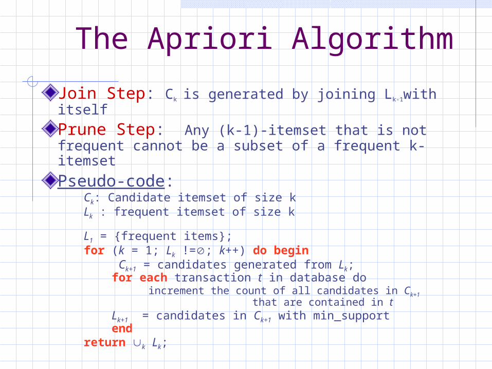
The Apriori Algorithm

Join Step: Ck is generated by joining Lk-1with itself

Prune Step: Any (k-1)-itemset that is not frequent cannot be a subset of a frequent k-itemset

Pseudo-code:Ck: Candidate itemset of size kLk : frequent itemset of size k

L1 = {frequent items};for (k = 1; Lk !=; k++) do begin Ck+1 = candidates generated from Lk; for each transaction t in database do

increment the count of all candidates in Ck+1 that are contained in t

Lk+1 = candidates in Ck+1 with min_support endreturn k Lk;

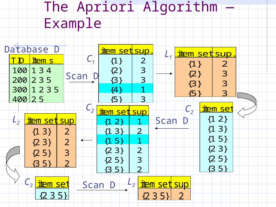
The Apriori Algorithm — Example

TID Items100 1 3 4200 2 3 5300 1 2 3 5400 2 5

Database D itemset sup.{1} 2{2} 3{3} 3{4} 1{5} 3

itemset sup.{1} 2{2} 3{3} 3{5} 3

Scan D

C1L1

itemset{1 2}{1 3}{1 5}{2 3}{2 5}{3 5}

itemset sup{1 2} 1{1 3} 2{1 5} 1{2 3} 2{2 5} 3{3 5} 2

itemset sup{1 3} 2{2 3} 2{2 5} 3{3 5} 2

L2

C2 C2Scan D

C3 L3itemset{2 3 5}

Scan D itemset sup{2 3 5} 2

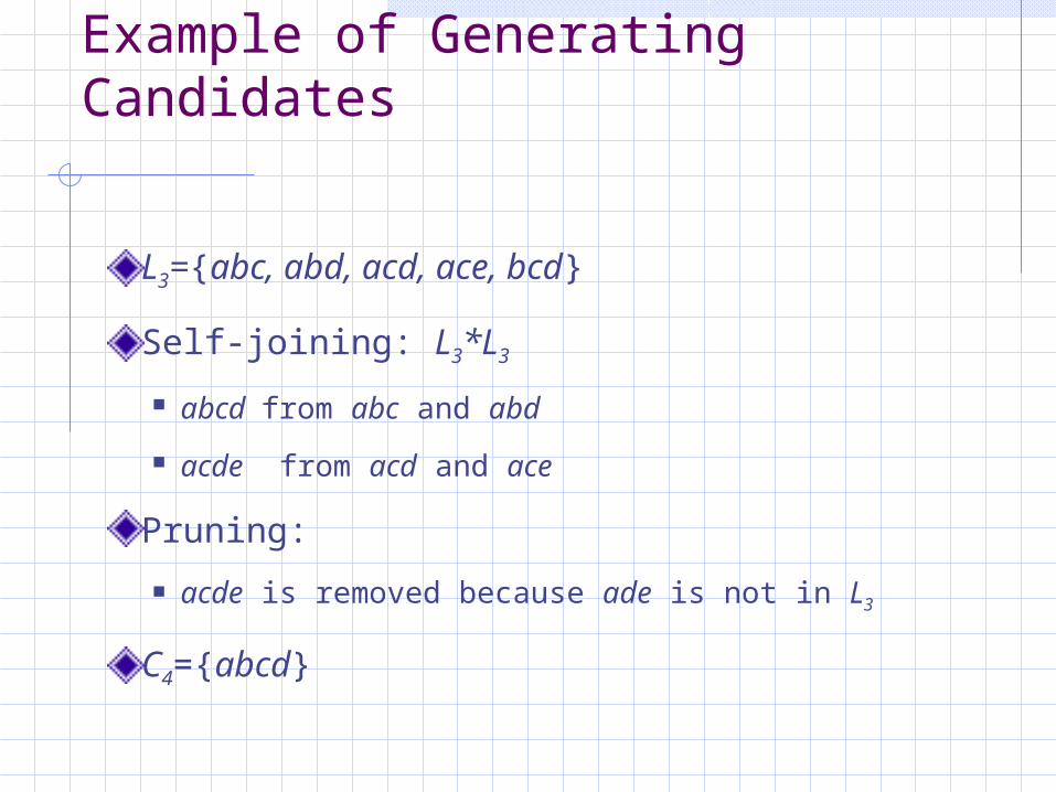
Example of Generating Candidates

L3={abc, abd, acd, ace, bcd}

Self-joining: L3*L3

abcd from abc and abd

acde from acd and ace

Pruning:

acde is removed because ade is not in L3

C4={abcd}

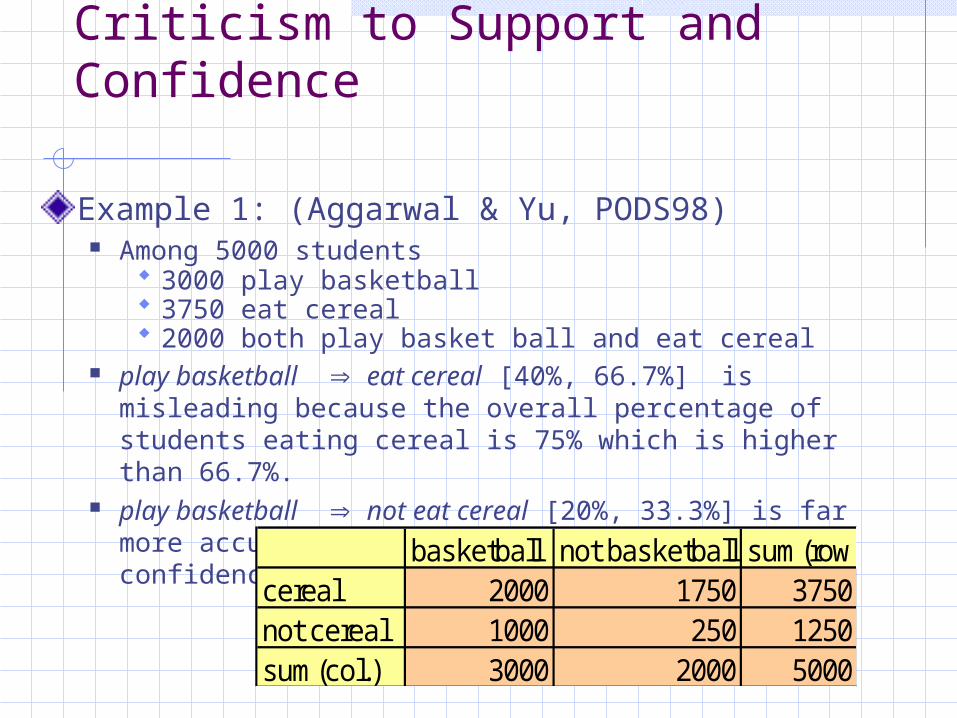
Criticism to Support and Confidence

Example 1: (Aggarwal & Yu, PODS98) Among 5000 students

3000 play basketball 3750 eat cereal 2000 both play basket ball and eat cereal

play basketball eat cereal [40%, 66.7%] is misleading because the overall percentage of students eating cereal is 75% which is higher than 66.7%.

play basketball not eat cereal [20%, 33.3%] is far more accurate, although with lower support and confidence

basketball not basketball sum(row)cereal 2000 1750 3750not cereal 1000 250 1250sum(col.) 3000 2000 5000

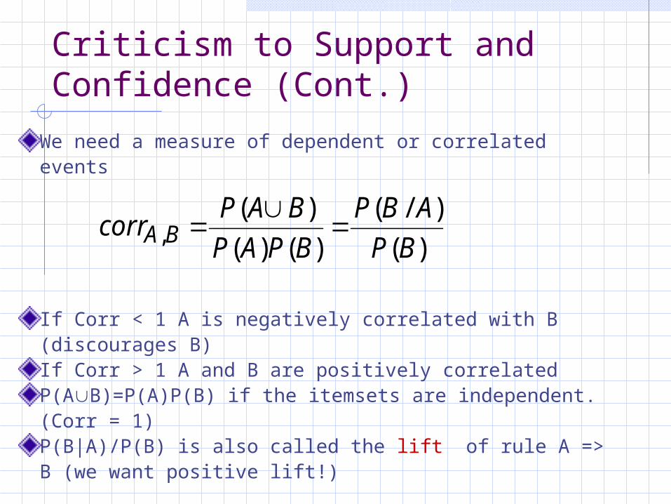
Criticism to Support and Confidence (Cont.)

We need a measure of dependent or correlated events

If Corr < 1 A is negatively correlated with B (discourages B)If Corr > 1 A and B are positively correlatedP(AB)=P(A)P(B) if the itemsets are independent. (Corr = 1)P(B|A)/P(B) is also called the lift of rule A => B (we want positive lift!)

)(

)/(

)()(

)(, BP

ABP

BPAP

BAPcorr BA

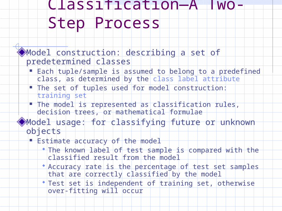
Classification—A Two-Step Process

Model construction: describing a set of predetermined classes

Each tuple/sample is assumed to belong to a predefined class, as determined by the class label attribute

The set of tuples used for model construction: training set The model is represented as classification rules, decision

trees, or mathematical formulae

Model usage: for classifying future or unknown objects

Estimate accuracy of the model The known label of test sample is compared with the

classified result from the model Accuracy rate is the percentage of test set samples

that are correctly classified by the model Test set is independent of training set, otherwise over-

fitting will occur

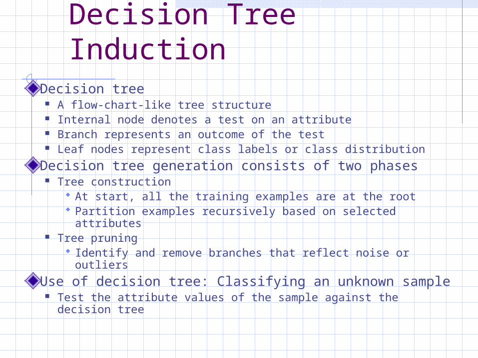
Classification by Decision Tree Induction

Decision tree A flow-chart-like tree structure Internal node denotes a test on an attribute Branch represents an outcome of the test Leaf nodes represent class labels or class distribution

Decision tree generation consists of two phases Tree construction

At start, all the training examples are at the root Partition examples recursively based on selected

attributes Tree pruning

Identify and remove branches that reflect noise or outliers

Use of decision tree: Classifying an unknown sample Test the attribute values of the sample against the decision

tree

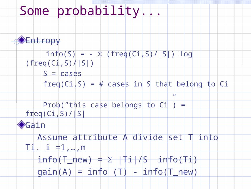
Some probability...

Entropy

info(S) = - (freq(Ci,S)/|S|) log (freq(Ci,S)/|S|)

S = cases freq(Ci,S) = # cases in S that belong to Ci

Prob(“this case belongs to Ci”) = freq(Ci,S)/|S|

Gain Assume attribute A divide set T into Ti. i

=1,…,m info(T_new) = |Ti|/S info(Ti) gain(A) = info (T) - info(T_new)

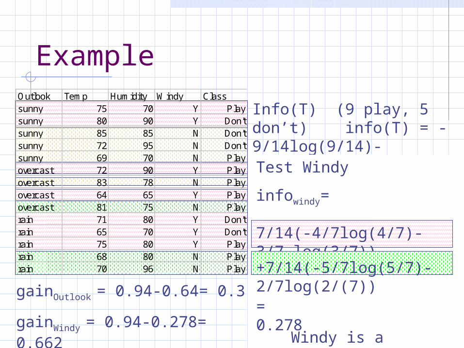
Example

Info(T) (9 play, 5 don’t) info(T) = -9/14log(9/14)- 5/14log(5/14) = 0.94 (bits)

Test: outlook

infoOutlook =

5/14 (-2/5 log(2/5)-3/5 log(3/5))+

4/14 (-4/4 log(4/4)) +

5/14 (-3/5 log(3/5) - 2/5 log(2/5))gainOutlook = 0.94-0.64= 0.3

= 0.64 (bits)

Test Windy

infowindy=

7/14(-4/7log(4/7)-3/7 log(3/7))

+7/14(-5/7log(5/7)-2/7log(2/(7))

= 0.278gainWindy = 0.94-0.278= 0.662

Windy is a better test

Outlook Temp Humidity Windy Classsunny 75 70 Y Playsunny 80 90 Y Don'tsunny 85 85 N Don'tsunny 72 95 N Don'tsunny 69 70 N Playovercast 72 90 Y Playovercast 83 78 N Playovercast 64 65 Y Playovercast 81 75 N Playrain 71 80 Y Don'train 65 70 Y Don'train 75 80 Y Playrain 68 80 N Playrain 70 96 N Play

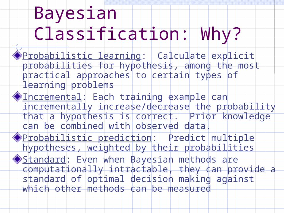
Bayesian Classification: Why?

Probabilistic learning: Calculate explicit probabilities for hypothesis, among the most practical approaches to certain types of learning problemsIncremental: Each training example can incrementally increase/decrease the probability that a hypothesis is correct. Prior knowledge can be combined with observed data.Probabilistic prediction: Predict multiple hypotheses, weighted by their probabilitiesStandard: Even when Bayesian methods are computationally intractable, they can provide a standard of optimal decision making against which other methods can be measured

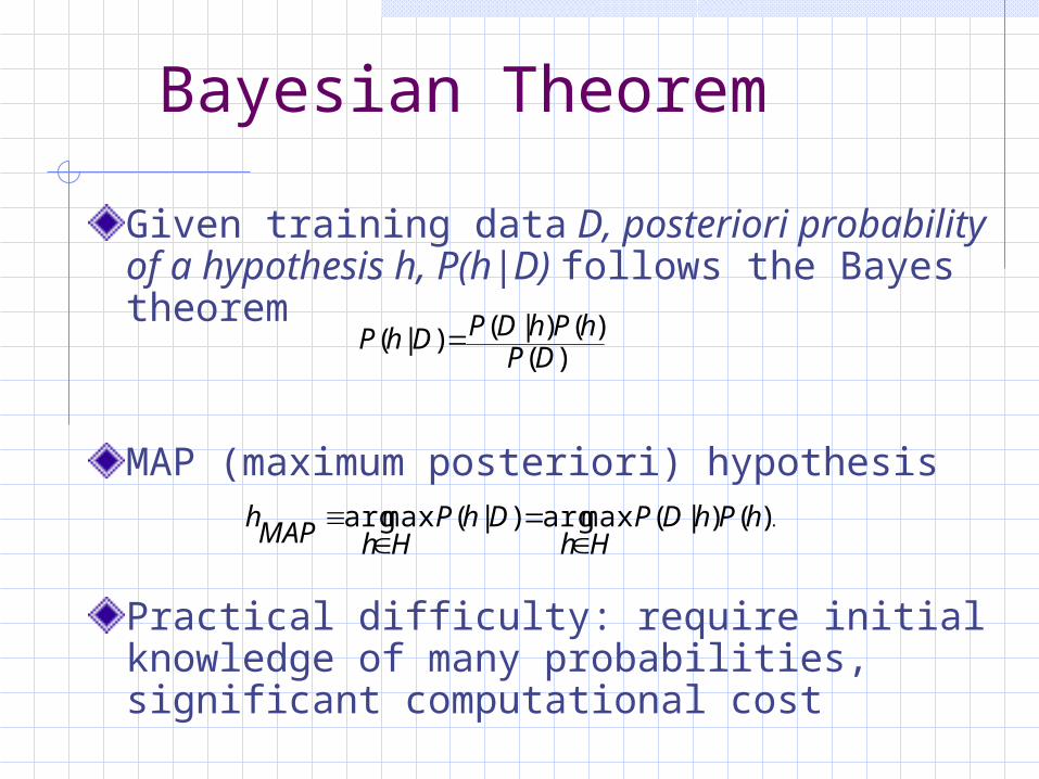
Bayesian Theorem

Given training data D, posteriori probability of a hypothesis h, P(h|D) follows the Bayes theorem

MAP (maximum posteriori) hypothesis

Practical difficulty: require initial knowledge of many probabilities, significant computational cost

)()()|()|(

DPhPhDPDhP

.)()|(maxarg)|(maxarg hPhDPHh

DhPHhMAP

h

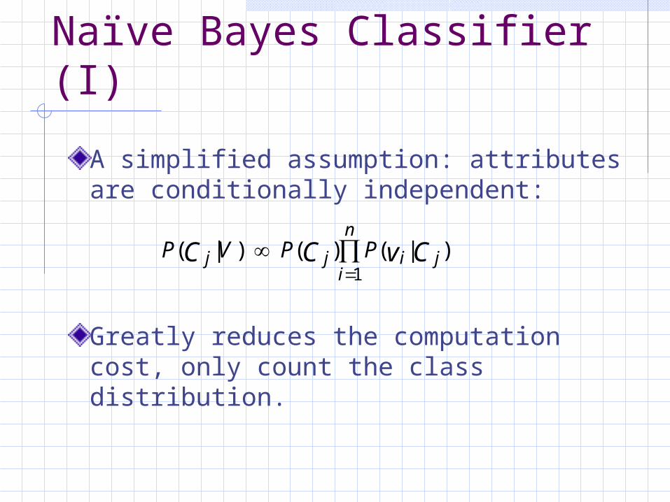
Naïve Bayes Classifier (I)

A simplified assumption: attributes are conditionally independent:

Greatly reduces the computation cost, only count the class distribution.

P V P Pj j i ji

n

C C v C( | ) ( ) ( | )

1

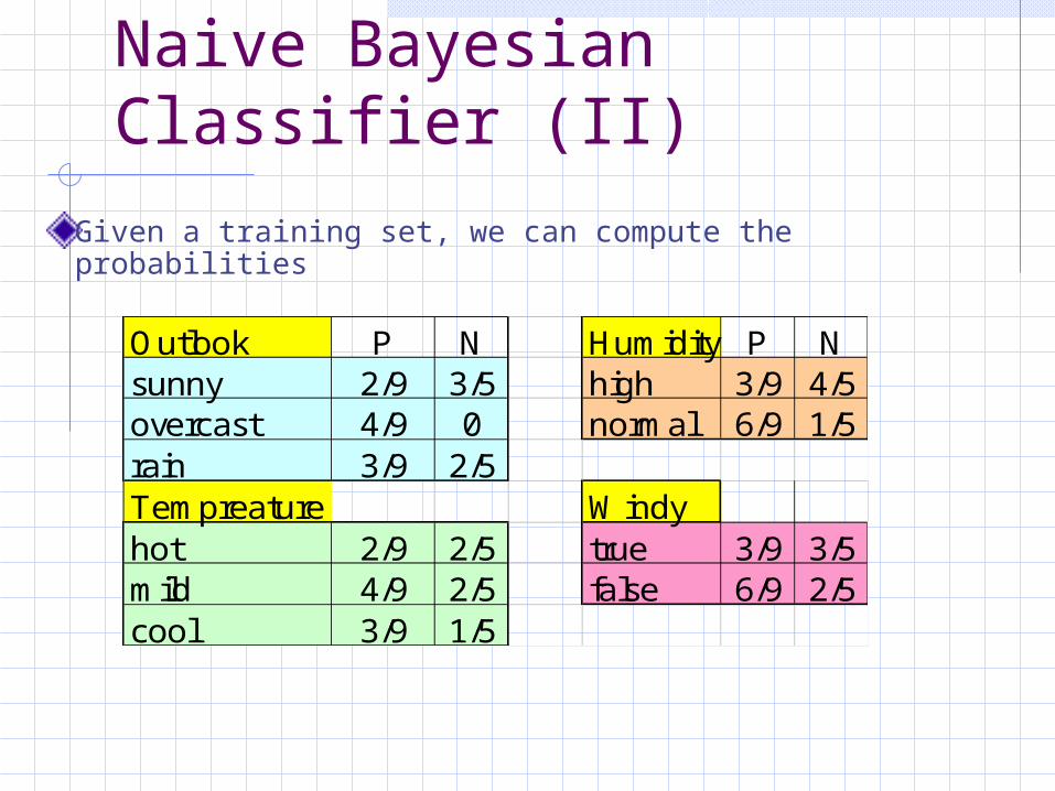
Naive Bayesian Classifier (II)

Given a training set, we can compute the probabilities

Outlook P N Humidity P Nsunny 2/9 3/5 high 3/9 4/5overcast 4/9 0 normal 6/9 1/5rain 3/9 2/5Tempreature Windyhot 2/9 2/5 true 3/9 3/5mild 4/9 2/5 false 6/9 2/5cool 3/9 1/5

3/9 x 3/9 x

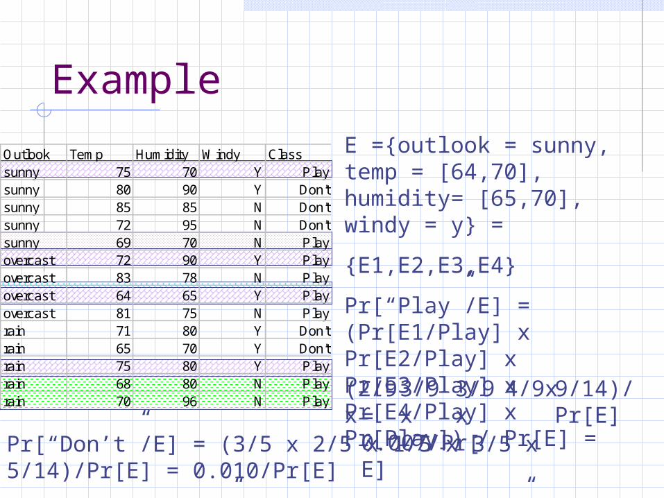
Example

E ={outlook = sunny, temp = [64,70], humidity= [65,70], windy = y} =

{E1,E2,E3,E4}

Pr[“Play”/E] = (Pr[E1/Play] x Pr[E2/Play] x Pr[E3/Play] x Pr[E4/Play] x Pr[Play]) / Pr[E] =(2/9x 4/9x

Outlook Temp Humidity Windy Classsunny 75 70 Y Playsunny 80 90 Y Don'tsunny 85 85 N Don'tsunny 72 95 N Don'tsunny 69 70 N Playovercast 72 90 Y Playovercast 83 78 N Playovercast 64 65 Y Playovercast 81 75 N Playrain 71 80 Y Don'train 65 70 Y Don'train 75 80 Y Playrain 68 80 N Playrain 70 96 N Play

9/14)/Pr[E]= 0.007/Pr[E]

Pr[“Don’t”/E] = (3/5 x 2/5 x 1/5 x 3/5 x 5/14)/Pr[E] = 0.010/Pr[E]

With E: Pr[“Play”/E] = 41 %, Pr[“Don’t”/E] = 59 %

Bayesian Belief Networks (I)FamilyHistory

LungCancer

PositiveXRay

Smoker

Emphysema

Dyspnea

LC

~LC

(FH, S) (FH, ~S)(~FH, S) (~FH, ~S)

0.8

0.2

0.5

0.5

0.7

0.3

0.1

0.9

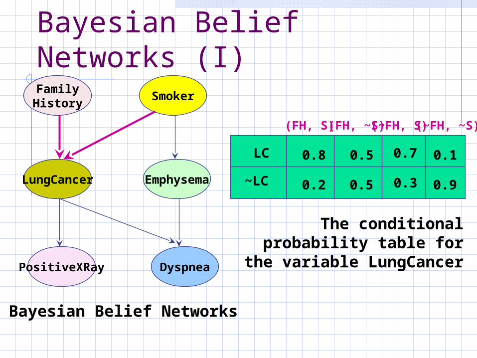
Bayesian Belief Networks

The conditional probability table for the variable LungCancer

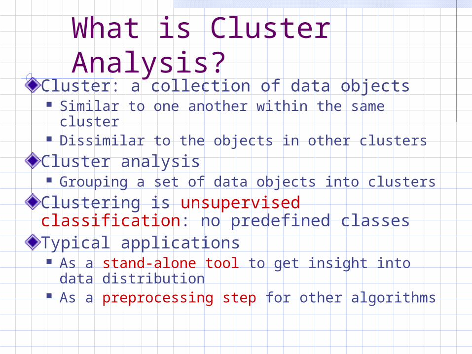
What is Cluster Analysis?Cluster: a collection of data objects Similar to one another within the same cluster Dissimilar to the objects in other clusters

Cluster analysis Grouping a set of data objects into clusters

Clustering is unsupervised classification: no predefined classesTypical applications As a stand-alone tool to get insight into data

distribution As a preprocessing step for other algorithms

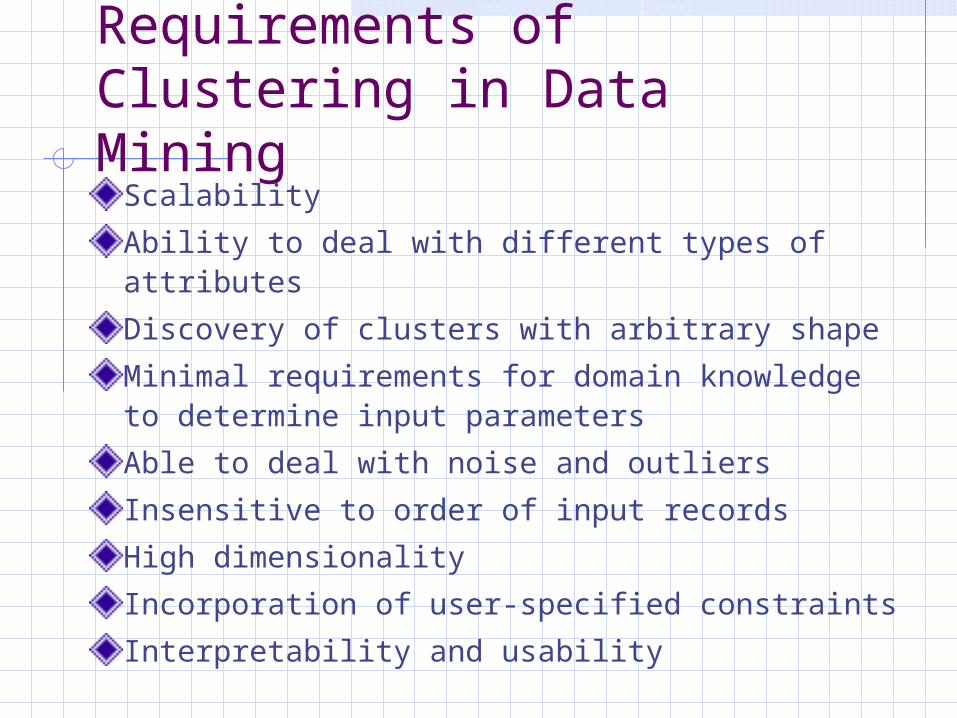
Requirements of Clustering in Data Mining

Scalability

Ability to deal with different types of attributes

Discovery of clusters with arbitrary shape

Minimal requirements for domain knowledge to determine input parameters

Able to deal with noise and outliers

Insensitive to order of input records

High dimensionality

Incorporation of user-specified constraints

Interpretability and usability

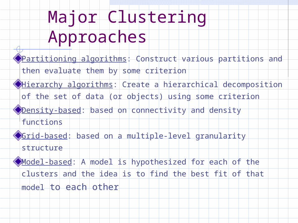
Major Clustering Approaches

Partitioning algorithms: Construct various partitions and

then evaluate them by some criterion

Hierarchy algorithms: Create a hierarchical decomposition

of the set of data (or objects) using some criterion

Density-based: based on connectivity and density functions

Grid-based: based on a multiple-level granularity structure

Model-based: A model is hypothesized for each of the

clusters and the idea is to find the best fit of that model to

each other

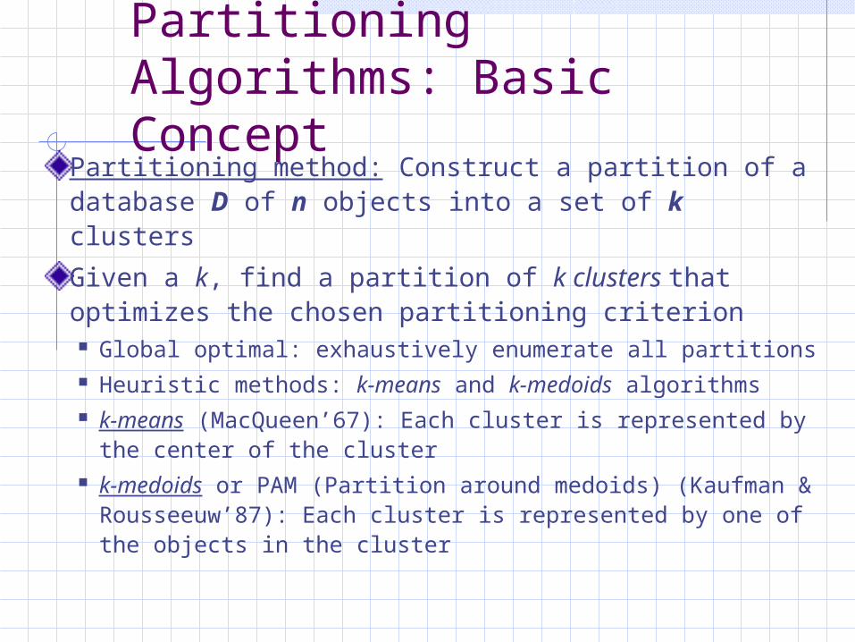
Partitioning Algorithms: Basic Concept

Partitioning method: Construct a partition of a database D of n objects into a set of k clusters

Given a k, find a partition of k clusters that optimizes the chosen partitioning criterion Global optimal: exhaustively enumerate all partitions Heuristic methods: k-means and k-medoids algorithms k-means (MacQueen’67): Each cluster is represented

by the center of the cluster k-medoids or PAM (Partition around medoids)

(Kaufman & Rousseeuw’87): Each cluster is represented by one of the objects in the cluster

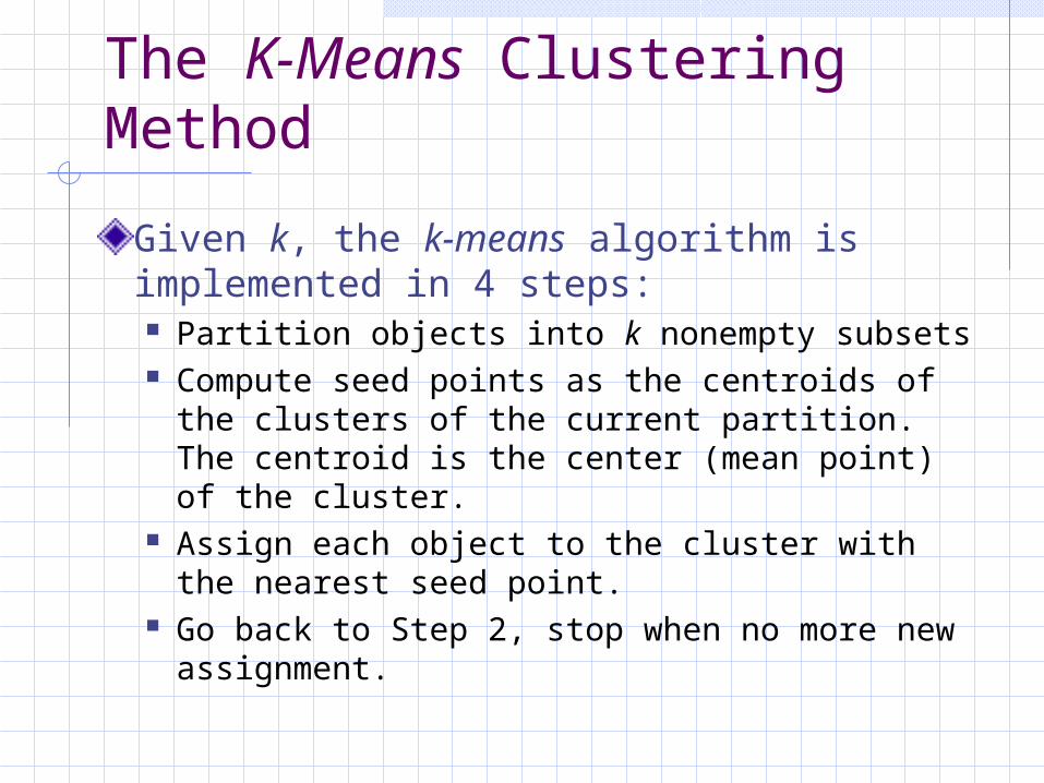
The K-Means Clustering Method

Given k, the k-means algorithm is implemented in 4 steps: Partition objects into k nonempty subsets Compute seed points as the centroids of the

clusters of the current partition. The centroid is the center (mean point) of the cluster.

Assign each object to the cluster with the nearest seed point.

Go back to Step 2, stop when no more new assignment.

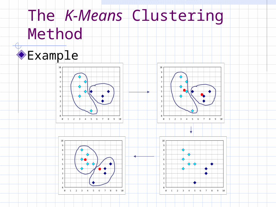
The K-Means Clustering Method

Example

0

1

2

3

4

5

6

7

8

9

10

0 1 2 3 4 5 6 7 8 9 10

0

1

2

3

4

5

6

7

8

9

10

0 1 2 3 4 5 6 7 8 9 10

0

1

2

3

4

5

6

7

8

9

10

0 1 2 3 4 5 6 7 8 9 10

0

1

2

3

4

5

6

7

8

9

10

0 1 2 3 4 5 6 7 8 9 10

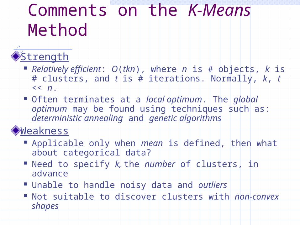
Comments on the K-Means Method

Strength Relatively efficient: O(tkn), where n is # objects, k is

# clusters, and t is # iterations. Normally, k, t << n. Often terminates at a local optimum. The global

optimum may be found using techniques such as: deterministic annealing and genetic algorithms

Weakness Applicable only when mean is defined, then what

about categorical data? Need to specify k, the number of clusters, in

advance Unable to handle noisy data and outliers Not suitable to discover clusters with non-convex

shapes

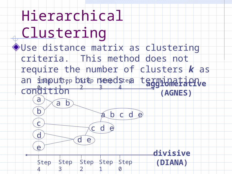
Hierarchical Clustering

Use distance matrix as clustering criteria. This method does not require the number of clusters k as an input, but needs a termination condition Step 0 Step 1 Step 2 Step 3 Step 4

b

d

c

e

a a b

d e

c d e

a b c d e

Step 4 Step 3 Step 2 Step 1 Step 0

agglomerative(AGNES)

divisive(DIANA)

More on Hierarchical Clustering Methods

Major weakness of agglomerative clustering methods do not scale well: time complexity of at least O(n2),

where n is the number of total objects can never undo what was done previously

Integration of hierarchical with distance-based clustering BIRCH (1996): uses CF-tree and incrementally

adjusts the quality of sub-clusters CURE (1998): selects well-scattered points from

the cluster and then shrinks them towards the center of the cluster by a specified fraction

CHAMELEON (1999): hierarchical clustering using dynamic modeling

Density-Based Clustering Methods

Clustering based on density (local cluster criterion), such as density-connected pointsMajor features: Discover clusters of arbitrary shape Handle noise One scan Need density parameters as termination

condition

Several interesting studies: DBSCAN: Ester, et al. (KDD’96) OPTICS: Ankerst, et al (SIGMOD’99). DENCLUE: Hinneburg & D. Keim (KDD’98) CLIQUE: Agrawal, et al. (SIGMOD’98)

Grid-Based Clustering Method

Using multi-resolution grid data structure

Several methods STING (a STatistical INformation Grid

approach) by Wang, Yang and Muntz (1997)

WaveCluster by Sheikholeslami, Chatterjee, and Zhang (VLDB’98)

CLIQUE: Agrawal, et al. (SIGMOD’98)

Self-Similar Clustering Barbará & Chen (2000)

Model-Based Clustering Methods

Attempt to optimize the fit between the data and some mathematical modelStatistical and AI approach Conceptual clustering

A form of clustering in machine learning Produces a classification scheme for a set of unlabeled

objects Finds characteristic description for each concept (class)

COBWEB (Fisher’87) A popular a simple method of incremental conceptual

learning Creates a hierarchical clustering in the form of a

classification tree Each node refers to a concept and contains a

probabilistic description of that concept

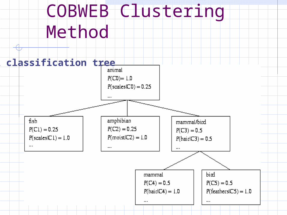
COBWEB Clustering Method

A classification tree

Summary

Association rule and frequent set miningClassification: decision tree, bayesian network, SVM, etc.Clustering algorithms can be categorized into partitioning methods, hierarchical methods, density-based methods, grid-based methods, and model-based methodsOther data mining tasks