Embed Size (px)
Citation preview

AN ABSTRACT OF THE THESIS OF Kathryn S. Pfretzschner for the degree of Master of Science in Wood Science and Civil Engineering presented on September 5, 2012 Title: Practical Modeling for Load Paths in a Realistic, Light-Frame Wood House Abstract approved:
Rakesh Gupta Thomas H. Miller
The objective of this study was to develop and validate practical modeling
methods for investigating load paths and system behavior in a realistic, light-frame wood
structure. The modeling methods were validated against full-scale tests on sub-
assemblies and an L-shaped house. The model of the L-shaped house was then modified
and used to investigate the effects of re-entrant corners, wall openings and gable-end
retrofits on system behavior and load paths. Results from this study showed that the
effects of adding re-entrant corners and wall openings on uplift load distributions were
dependent on the orientation of the trusses with respect to the walls. Openings added to
walls parallel to the trusses had the least effect on loads carried by the remaining walls in
the building. Varying re-entrant corner dimensions of the L-shaped house under ASCE
7-05 (ASCE 2005) design wind loads caused increasing degrees of torsion throughout the
house, depending on the relative location and stiffness of the in-plane walls (parallel to
the applied wind loads) as well as the assumed direction of the wind loads. Balancing the
stiffness of the walls on either side of the house with the largest re-entrant corner helped
to decrease torsion in the structure somewhat. Finally, although previous full-scale tests
on gable-end sections verified the effectiveness of the gable-end retrofit that was recently
adopted into the 2010 Florida building code, questions remained about the effects of the
retrofit on torsion in a full building. The current study found that adding the gable-end
retrofits to the L-shaped house did not cause additional torsion.

Copyright by Kathryn S. Pfretzschner September 5, 2012
All Rights Reserved

Practical Modeling for Load Paths in a Realistic, Light-Frame Wood House
by Kathryn S. Pfretzschner
A THESIS
submitted to
Oregon State University
in partial fulfillment of the requirements for the
degree of
Master of Science
Presented: September 5, 2012 Commencement Date: June 2013

Master of Science thesis of Kathryn S. Pfretzschner presented on September 5, 2012. APPROVED: Co-Major Professor representing Wood Science and Engineering Co-Major Professor representing Civil Engineering Head of the Department of Wood Science and Engineering Acting Head of the School of Civil and Construction Engineering Dean of the Graduate School I understand that my thesis will become part of the permanent collection of Oregon State University libraries. My signature below authorizes release of my thesis to any reader upon request.
Kathryn S. Pfretzschner, Author

ACKNOWLEDGMENTS
I would like to express my appreciation to the following people and organizations:
• My advisors, Dr. Rakesh Gupta and Dr. Thomas H. Miller, for their help,
guidance and patience during the course of this project.
• Kenneth Martin, Dr. Phillip Paevere and Dr. Bohumil Kasal whose previous
research and development made this project possible. I am especially thankful for
Kenneth Martin, who proposed this project and instructed me in the design of
wood structures.
• The Department of Wood Science & Engineering and the School of Civil &
Construction Engineering at Oregon State University for providing the necessary
resources and furthering my education.
• The Oregon State University Center for Wood Utilization Research for funding
this project.
Finally, I would not have made it this far without my family. My parents, Janet and
Richard Pfretzschner, provided the support and encouragement that kept me going
throughout my undergraduate and graduate degrees. Also my older brother, Paul
Pfretzschner, inspired me to pursue engineering through his own academic
accomplishments in science and mathematics.

CONTRIBUTION OF AUTHORS
Dr. Rakesh Gupta and Dr. Thomas H. Miller provided technical guidance and support
during the research stages. They also provided insight and editing for the final
manuscript.

TABLE OF CONTENTS Page
INTRODUCTION .............................................................................................................. 1
OBJECTIVES ................................................................................................................. 1
RESEARCH APPROACH ............................................................................................. 2
MANUSCRIPT: PRACTICAL MODELING FOR LOAD PATHS IN A REALISTIC, LIGHT-FRAME WOOD HOUSE ...................................................................................................................... 4
ABSTRACT .................................................................................................................... 5
INTRODUCTION .......................................................................................................... 5
RESEARCH METHODS ............................................................................................... 7
Modeling Methods ...................................................................................................... 7
Model Validation Procedure ..................................................................................... 10
RESULTS AND DISCUSSION ................................................................................... 18
Model Validation ...................................................................................................... 18
Uniform Uplift Investigation .................................................................................... 20
Wind Load Investigation........................................................................................... 23
CONCLUSIONS........................................................................................................... 27
ACKNOWLEDGMENTS ............................................................................................ 28
REFERENCES ............................................................................................................. 29
CONCLUSIONS AND RECOMMENDATIONS ........................................................... 32
BIBLIOGRAPHY ............................................................................................................. 34

LIST OF FIGURES Figure Page
Figure 1: (a) Floor Plan with Centerline Dimensions [m (ft-in)] and Wall Designation, (b) Wall framing (mm) (Paevere 2002) ............................................................................ 11
Figure 2: Truss Orientation and Gable-End Framing ...................................................... 12
Figure 3: Plywood Sheathing on Exterior of Walls 5 and 9 (Paevere et al. 2003) .......... 13
Figure 4: G12 vs. Wall Length for Plywood and GWB Wall Sheathing .......................... 14
Figure 5: Modified Gable-End Framing for Load Path Investigations ............................ 15
Figure 6: Wind Directions and ASCE 7-05 Load Cases.................................................. 17
Figure 7: Example C-Shaped Gable-End Retrofit at Gable-End Stud ............................. 18
Figure 8: Load Distribution Plot for Paevere et al. (2003) Load Case 4 ......................... 20
Figure 9: Uplift Reactions for Rectangular (Left) and L-shaped (Right) Index Buildings........................................................................................................................................... 21
Figure 10: Change in Uplift Reactions (Magnified 4x) due to Openings in Wall 2 (Left) and Wall 4 (Right) ............................................................................................................ 22
Figure 11: Uplift Reactions in L-Shaped Index House .................................................... 23
Figure 12: Lateral Load Distribution and Top Plate Deflected Shapes for Re-Entrant Corner Variations .............................................................................................................. 26
Figure 13: Displaced Shape of Large Re-Entrant Corner Building with Increased Stiffness in Walls 1 and 2 ................................................................................................. 27

LIST OF TABLES Table Page
Table 1: Sheathing Material Properties............................................................................ 13
Table 2: Material Densities used for Building Self-Weight ............................................ 14

LIST OF APPENDICES
Appendix Page
APPENDIX A: EXTENDED LITERATURE REVIEW ............................................................ 39
APPENDIX B: TWO-DIMENSIONAL TRUSS MODEL VALIDATION ................................... 54
APPENDIX C: THREE DIMENSIONAL ROOF ASSEMBLY MODEL VALIDATION ................ 62
APPENDIX D: PLOTS FOR ROOF ASSEMBLY MODEL VALIDATION ................................. 71
APPENDIX E: TWO-DIMENSIONAL SHEAR WALL MODEL VALIDATION ........................ 95
APPENDIX F: SHEATHING G12 ADJUSTMENT PROCEDURE FOR EDGE NAIL SPACING .. 106
APPENDIX G: DETAILS FOR FULL BUILDING MODEL OF PAEVERE ET AL. (2003) HOUSE......................................................................................................................................... 112
APPENDIX H: FULL BUILDING MODEL VALIDATION ................................................... 123
APPENDIX I: MODEL VARIATIONS USED IN UPLIFT AND WIND LOAD INVESTIGATIONS......................................................................................................................................... 144
APPENDIX J: UNIFORM UPLIFT INVESTIGATION .......................................................... 152
APPENDIX K: ASCE 7-05 DESIGN LOADS USED FOR WIND LOAD INVESTIGATION .... 162
APPENDIX L: WIND LOAD INVESTIGATION ................................................................. 168

LIST OF APPENDIX FIGURES
Figure Page
Figure B-1: 6:12 Truss Geometry .....................................................................................55
Figure B-2: 3:12 Truss Geometry .....................................................................................55
Figure B-3: Connectivity and Element Labels for 2D Truss Model .................................56
Figure C-1: Pattern of Truss Stiffness in Assemblies ........................................................62
Figure C-2: Local Coordinate Orientation of Thick Shell Elements for Sheathing .........64
Figure C-3: Hooke’s Law for Orthotropic Materials .........................................................65
Figure C-4: “Roller-Roller” Support Conditions ..............................................................67
Figure C-5: Locations for Deflection Measurement on Each Truss .................................68
Figure D-1: Relative Reactions for 3:12 Truss Assembly When Truss 1 is Loaded ........71
Figure D-2: Relative Reactions for 3:12 Truss Assembly When Truss 2 is Loaded ........72
Figure D-3: Relative Reactions for 3:12 Truss Assembly When Truss 3 is Loaded ........73
Figure D-4: Relative Reactions for 3:12 Truss Assembly When Truss 4 is Loaded ........73
Figure D-5: Relative Reactions for 3:12 Truss Assembly When Truss 5 is Loaded ........73
Figure D-6: Relative Reactions for 3:12 Truss Assembly When Truss 6 is Loaded ........74
Figure D-7: Relative Reactions for 3:12 Truss Assembly When Truss 7 is Loaded ........74
Figure D-8: Relative Reactions for 3:12 Truss Assembly When Truss 8 is Loaded ........75
Figure D-9: Relative Reactions for 3:12 Truss Assembly When Truss 9 is Loaded ........75
Figure D-10: Relative Reactions for 6:12 Truss Assembly When Truss 1 is Loaded ......77
Figure D-11: Relative Reactions for 6:12 Truss Assembly When Truss 2 is Loaded ......77
Figure D-12: Relative Reactions for 6:12 Truss Assembly When Truss 3 is Loaded ......78
Figure D-13: Relative Reactions for 6:12 Truss Assembly When Truss 4 is Loaded ......78
Figure D-14: Relative Reactions for 6:12 Truss Assembly When Truss 5 is Loaded ......79
Figure D-15: Relative Reactions for 6:12 Truss Assembly When Truss 6 is Loaded ......79

LIST OF APPENDIX FIGURES (Continued)
Figure Page
Figure D-16: Relative Reactions for 6:12 Truss Assembly When Truss 7 is Loaded ......80
Figure D-17: Relative Reactions for 6:12 Truss Assembly When Truss 8 is Loaded ......80
Figure D-18: Relative Reactions for 6:12 Truss Assembly When Truss 9 is Loaded ......81
Figure D-19: Relative Deflections for 3:12 Truss Assembly When Truss 1 is Loaded ...83
Figure D-20: Relative Deflections for 3:12 Truss Assembly When Truss 2 is Loaded ...84
Figure D-21: Relative Deflections for 3:12 Truss Assembly When Truss 3 is Loaded ...84
Figure D-22: Relative Deflections for 3:12 Truss Assembly When Truss 4 is Loaded ...85
Figure D-23: Relative Deflections for 3:12 Truss Assembly When Truss 5 is Loaded ...85
Figure D-24: Relative Deflections for 3:12 Truss Assembly When Truss 6 is Loaded ....86
Figure D-25: Relative Deflections for 3:12 Truss Assembly When Truss 7 is Loaded ....86
Figure D-26: Relative Deflections for 3:12 Truss Assembly When Truss 8 is Loaded ...87
Figure D-27: Relative Deflections for 3:12 Truss Assembly When Truss 9 is Loaded ...87
Figure D-28: Relative Deflections for 6:12 Truss Assembly When Truss 1 is Loaded ...89
Figure D-29: Relative Deflections for 6:12 Truss Assembly When Truss 2 is Loaded ...89
Figure D-30: Relative Deflections for 6:12 Truss Assembly When Truss 3 is Loaded ...90
Figure D-31: Relative Deflections for 6:12 Truss Assembly When Truss 4 is Loaded ...90
Figure D-32: Relative Deflections for 6:12 Truss Assembly When Truss 5 is Loaded ...91
Figure D-33: Relative Deflections for 6:12 Truss Assembly When Truss 6 is Loaded ...91
Figure D-34: Relative Deflections for 6:12 Truss Assembly When Truss 7 is Loaded ...92
Figure D-35: Relative Deflections for 6:12 Truss Assembly When Truss 8 is Loaded ...92
Figure D-36: Relative Deflections for 6:12 Truss Assembly When Truss 9 is Loaded ...93
Figure E-1: Testing Apparatus and Sensor Locations (Dolan and Johnson 1996) ...........97

LIST OF APPENDIX FIGURES (Continued)
Figure Page
Figure E-2: Example of Assumed Wall Framing with SAP2000 Wire Frame Overlay for Type D Shear Wall ............................................................................................................99
Figure E-3: Example Frame Section Assignment for Type D Shear Wall ......................99
Figure E-4: Local Axes for Anchor Bolts and Hold-downs (Martin 2010) ....................102
Figure E-5: Anchor Bolt and Hold-Down Placement in SAP2000 Model ....................102
Figure F-1: (Top) framing plan for example calibration (grey studs are single studs) and (Bottom) support and loading conditions for calibration model .....................................107
Figure F-2: Sheathing G12 vs. Shear Wall Deflection in SAP2000 for Example Calibration Model ...........................................................................................................109
Figure F-3: AF&PA (2005b) Predicted Deflection and Required G12 in SAP2000 vs. Wall Length ....................................................................................................................111
Figure G-1: G12 vs. Wall Length for 9.5 mm Plywood and 13 mm GWB Sheathing ..115
Figure G-2: Anchor Bolt and Load Sensor Placement (Paevere 2002) ..........................116
Figure G-3: Wall Locations Used in SAP2000 Model – m (ft-in) .................................116
Figure G-4: Wall Configurations (Paevere 2002) ..........................................................117
Figure G-5: Wall 3 Configuration used for SAP2000 Model ........................................118
Figure G-6: Wall Framing (Paevere 2002) .....................................................................118
Figure G-7: Example of Assumed Framing with SAP2000 Wire Frame Overlay for Wall 2........................................................................................................................................119
Figure G-8: Example Frame Section Assignment for Wall 2 .........................................119
Figure G-9: Assumed Framing with SAP2000 Wire Frame Overlay for Type A Trusses ..........................................................................................................................................120
Figure G-10: Assumed Framing with SAP2000 Wire Frame Overlay for Type B Trusses ..........................................................................................................................................120
Figure G-11: Example Frame Section Assignment used for Trusses .............................120
Figure G-12: Truss Layout for Type A and Type B Trusses ..........................................121
LIST OF APPENDIX FIGURES (Continued)
Figure Page
Figure G-13: 2-Joint Links used to Connect Wall 3 to Truss Bottom Chords ...............121
Figure G-14: Gable-End Overhang Framing used in SAP2000 Model ..........................122
Figure G-15: Gable-End Sheathing Placement used in SAP2000 Model .......................123
Figure H-1: Load Case 2 – 2.78 kN Applied to Top-Plate at Wall 1 ..............................124
Figure H-2: Lateral Load Distribution to E-W Walls (Load Case 2) ..............................124
Figure H-3: Load Case 3 – 4.79 kN Applied to Top-Plate at Wall 2 ..............................125
Figure H-4: Lateral Load Distribution to E-W Walls (Load Case 3) ..............................125
Figure H-5: Load Case 4 – 4.92 kN Applied to Top-Plate at Wall 3 ..............................126
Figure H-6: Lateral Load Distribution to E-W Walls (Load Case 4) ..............................127
Figure H-7: Load Case 5 – 4.92 kN Applied to Top-Plate at Wall 4 ..............................127
Figure H-8: Lateral Load Distribution to E-W Walls (Load Case 5) ..............................127
Figure H-9: Load Case 6 – 5.18 kN Applied to Top-Plate at Wall 8 ..............................128
Figure H-10: Lateral Load Distribution to N-S Walls (Load Case 6) .............................128
Figure H-11: Load Case 7 – 5.07 kN Applied to Top-Plate at Wall 2 and 5.13 kN Applied to Top-Plate at Wall 8 ......................................................................................................129
Figure H-12: Lateral Load Distribution to E-W Walls (Load Case 7) ............................129
Figure H-13: Lateral Load Distribution to N-S Walls (Load Case 7) .............................130
Figure H-14: Load Case 8 – 5.16 kN Applied to Top-Plate at Wall 5 ............................131
Figure H-15: Lateral Load Distribution to N-S Walls (Load Case 8) .............................131
Figure H-16: Load Case 9 – 8.04 kN Applied to Top-Plate at Wall 4 and 5.17 kN Applied to Top-Plate at Wall 5 ......................................................................................................132
Figure H-17: Lateral Load Distribution to E-W Walls (Load Case 9) ............................132
Figure H-18: Lateral Load Distribution to N-S Walls (Load Case 9) .............................133

LIST OF APPENDIX FIGURES (Continued)
Figure Page
Figure H-19: Load Case 10 – 5.12 kN Applied to Top-Plate at Wall 2 and 3.18 kN Applied to Top-Plate at Wall 5 ........................................................................................134
Figure H-20: Lateral Load Distribution to E-W Walls (Load Case 10) ..........................134
Figure H-21: Lateral Load Distribution to N-S Walls (Load Case 10) ...........................135
Figure H-22: Load Case 11 – 6.80 kN Applied to Top-Plate between Walls 2 and 3 .....136
Figure H-23: Lateral Load Distribution to E-W Walls (Load Case 11) ..........................136
Figure H-24: Load Case 12 – 1.10 kN, 5.43 kN, 15.0 kN and 6.50 kN Applied to Top-Plate at Walls 1, 2, 3 and 4, respectively ........................................................................137
Figure H-25: Lateral Load Distribution to E-W Walls (Load Case 12) ..........................137
Figure H-26: Load Case 13 – 5.09 kN Applied to Roof Ridge of East Gable-End (at -5 degrees) ...........................................................................................................................138
Figure H-27: Lateral Load Distribution to E-W Walls (Load Case 13) ..........................138
Figure H-28: Lateral Load Distribution to N-S Walls (Load Case 13) ...........................139
Figure H-29: Load Case 14 – 5.21 kN Applied to Roof Ridge of East Gable-End (at -10 degrees) ............................................................................................................................140
Figure H-30: Lateral Load Distribution to E-W Walls (Load Case 14) ..........................140
Figure H-31: Lateral Load Distribution to N-S Walls (Load Case 14) ...........................141
Figure H-32: Load Case 15 – 2.80 kN Applied to Roof Ridge of East Gable-End (at 20 degrees) ............................................................................................................................142
Figure H-33: Lateral Load Distribution to E-W Walls (Load Case 15) ..........................142
Figure H-34: Lateral Load Distribution to N-S Walls (Load Case 15) ...........................143
Figure I-1: Gable End-Framing and Sheathing Modifications for Uplift and Wind Load Investigations ..................................................................................................................145
Figure I-2: Progression of Building Variations Used in Uplift Investigation ................145
Figure I-3: Rectangular Index Building for Uplift Investigation ...................................146
Figure I-4: L-Shaped Index Building for Uplift Investigation ........................................146
LIST OF APPENDIX FIGURES (Continued)
Figure Page
Figure I-5: Framing Detail for Openings used in Uplift Investigation ..........................147
Figure I-6: Locations of Openings Used for Uplift Investigation ...................................147
Figure I-7: Progression of Building Variations Used in Wind Load Investigation ........148
Figure I-8: L-Shaped Index House for Wind Load Investigation ...................................148
Figure I-9: Gable-End Retrofit Detail from 2010 Florida Building Code (ICC 2011) ...149
Figure I-10: Gable-End Studs + Retrofit Studs Modeled with L-Shaped Cross-Section ..........................................................................................................................................149
Figure I-11: Example of Gable-End Retrofit in the Model ............................................150
Figure I-12: Re-Entrant Corner Variations Used in Wind Load Investigation ...............150
Figure I-13: Re-Entrant Corner Variation Dimensions for Wind Load Investigation ....151
Figure J-1: Uplift Reactions for Rectangular Index Building under Uniform Uplift Pressure ...........................................................................................................................153
Figure J-2: Uplift Reactions for L-Shaped Index Building under Uniform Uplift Pressure ..........................................................................................................................................153
Figure J-3: Difference in Uplift Reactions between Rectangular and L-Shaped Index Buildings under Uniform Uplift Pressure .......................................................................154
Figure J-4: Uplift Reactions for L-Shaped Building with Opening in Wall 2 (under Uniform Uplift Pressure) .................................................................................................155
Figure J-5: Difference in Uplift Reactions due to Opening in Wall 2 .............................155
Figure J-6: Uplift Reactions for L-Shaped Building with Opening in Wall 4 (under Uniform Uplift Pressure) .................................................................................................156
Figure J-7: Difference in Uplift Reactions due to Opening in Wall 4 .............................156
Figure J-8: Uplift Reactions for L-Shaped Building with Opening in Wall 9, Centered Under Gable-End (under Uniform Uplift Pressure) .........................................................157
Figure J-9: Difference in Uplift Reactions due to Opening in Wall 9, Centered Under Gable-End .......................................................................................................................157

LIST OF APPENDIX FIGURES (Continued)
Figure Page
Figure J-10: Uplift Reactions for L-Shaped Building with Opening in Wall 9, Opposite Re-Entrant Corner (under Uniform Uplift Pressure ........................................................158
Figure J-11: Difference in Uplift Reactions due to Opening in Wall 9, Opposite Re-Entrant Corner .................................................................................................................158
Figure J-12: Uplift Reactions for L-Shaped Building with GWB (under Uniform Uplift Pressure) ...........................................................................................................................159
Figure J-13: Difference in Uplift Reactions from L-Shaped Building due to addition of GWB ...............................................................................................................................159
Figure J-14: Uplift Reactions for L-Shaped Building with Opening in Wall 2 and GWB (under Uniform Uplift Pressure) ......................................................................................160
Figure J-15: Difference in Uplift Reactions in L-Shaped Building with Opening in Wall 2 Due to Addition of GWB ................................................................................................160
Figure J-16: Uplift Reactions for L-Shaped Building with Opening in Wall 9 and GWB (under Uniform Uplift Pressure) ......................................................................................161
Figure J-17: Difference in Uplift Reactions in L-Shaped Building with Opening in Wall 9 Due to Addition of GWB ................................................................................................161
Figure K-1: Wind Directions Considered for Wind Load Investigation ........................162
Figure K-2: ASCE 7-05 Design Wind Load Cases for Main Wind Force Resisting System, Method 2 (ASCE 7-05 Figure 6-9) ...................................................................163
Figure K-3: Surface Designations used for Wind Pressure Calculations ......................164
Figure L-1: Uplift Reactions for L-shaped index house under North-South Wind Loads ..........................................................................................................................................169
Figure L-2: Lateral Load Distribution to North-South walls under North-South Wind Loads ................................................................................................................................169
Figure L-3: Uplift Reactions for L-shaped index house under West-East Wind Loads .170
Figure L-4: Lateral Load Distribution to East-West walls under West-East Wind Loads ..........................................................................................................................................170
Figure L-5: Uplift Reactions for L-shaped index house under Southeast-Northwest Wind Loads ...............................................................................................................................171

LIST OF APPENDIX FIGURES (Continued)
Figure Page
Figure L-6: Lateral Load Distribution to North-South walls under Southeast-Northwest Wind Loads .....................................................................................................................171
Figure L-7: Lateral Load Distribution to East-West walls under Southeast-Northwest Wind Loads .....................................................................................................................172
Figure L-8: Uplift Reactions for Building with Gable-End Retrofits under North-South Wind Loads .....................................................................................................................173
Figure L-9: Difference in Uplift Reactions between Building with Gable-End Retrofits and L-shaped index house under North-South Wind Loads ...........................................173
Figure L-10: Lateral Load Distribution to North-South walls under North-South Wind Loads ...............................................................................................................................174
Figure L-11: Uplift Reactions for Building with Gable-End Retrofits under West-East Wind Loads .....................................................................................................................175
Figure L-12: Difference in Uplift Reactions between Building with Gable-End Retrofits and L-shaped index house under West-East Wind Loads ..............................................175
Figure L-13: Lateral Load Distribution to East-West walls under West-East Wind Loads ..........................................................................................................................................176
Figure L-14: Uplift Reactions for Building with Gable-End Retrofits under Southeast-Northwest Wind Loads ...................................................................................................177
Figure L-15: Difference in Uplift Reactions between Building with Gable-End Retrofits and L-shaped index house under Southeast-Northwest Wind Loads .............................177
Figure L-16: Lateral Load Distribution to East-West walls under Southeast-Northwest Wind Loads .....................................................................................................................178
Figure L-17: Lateral Load Distribution to North-South walls under Southeast-Northwest Wind Loads .....................................................................................................................178
Figure L-18: Uplift Reactions for Building with Small Re-Entrant Corner under North-South Wind Loads ...........................................................................................................179
Figure L-19: Difference in Uplift Reactions between Building with Small Re-Entrant Corner and L-shaped index house under North-South Wind Loads ...............................179
Figure L-20: Uplift Reactions for Building with Medium Re-Entrant Corner under North-South Wind Loads ...........................................................................................................180

LIST OF APPENDIX FIGURES (Continued)
Figure Page
Figure L-21: Difference in Uplift Reactions between Building with Medium Re-Entrant Corner and L-shaped index house under North-South Wind ..........................................180
Figure L-22: Uplift Reactions for Building with Large Re-Entrant Corner under North-South Wind Loads ...........................................................................................................181
Figure L-23: Difference in Uplift Reactions between Building with Large Re-Entrant Corner and L-shaped index house under North-South Wind Loads ...............................181
Figure L-24: Lateral Load Distribution to North-South walls under North-South Wind Loads ...............................................................................................................................182
Figure L-25: Unit Shear in North-South walls under North-South Wind Loads ............182
Figure L-26: Uplift Reactions for Building with Small Re-Entrant Corner under West-East Wind Loads .............................................................................................................183
Figure L-27: Difference in Uplift Reactions between Building with Small Re-Entrant Corner and L-shaped index house under West-East Wind Loads ..................................183
Figure L-28: Uplift Reactions for Building with Medium Re-Entrant Corner under West-East Wind Loads .............................................................................................................184
Figure L-29: Difference in Uplift Reactions between Building with Medium Re-Entrant Corner and L-shaped index house under West-East Wind Loads ..................................184
Figure L-30: Uplift Reactions for Building with Large Re-Entrant Corner under West-East Wind Loads .............................................................................................................185
Figure L-31: Difference in Uplift Reactions between Building with Large Re-Entrant Corner and L-shaped index house under West-East Wind Loads ..................................185
Figure L-32: Lateral Load Distribution to East-West walls under West-East Wind Loads ..........................................................................................................................................186
Figure L-33: Uplift Reactions for Building with Small Re-Entrant Corner under Southeast-Northwest Wind Loads ..................................................................................187
Figure L-34: Difference in Uplift Reactions between Building with Small Re-Entrant Corner and L-shaped index house under Southeast-Northwest Wind Loads (with Self Weight) ...........................................................................................................................187
Figure L-35: Uplift Reactions for Building with Medium Re-Entrant Corner under Southeast-Northwest Wind Loads ..................................................................................188

LIST OF APPENDIX FIGURES (Continued)
Figure Page
Figure L-36: Difference in Uplift Reactions between Building with Medium Re-Entrant Corner and L-shaped index house under Southeast-Northwest Wind Loads .................188
Figure L-37: Uplift Reactions for Building with Large Re-Entrant Corner under Southeast-Northwest Wind Loads ..................................................................................189
Figure L-38: Difference in Uplift Reactions between Building with Large Re-Entrant Corner and L-shaped index house under Southeast-Northwest Wind Loads .................189
Figure L-39: Lateral Load Distribution to East-West walls under Southeast-Northwest Wind Loads .....................................................................................................................190
Figure L-40: Lateral Load Distribution to North-South walls under Southeast-Northwest Wind Loads .....................................................................................................................190
Figure L-41: Unit Shear in North-South walls under Southeast-Northwest Wind Loads ..........................................................................................................................................191

LIST OF APPENDIX TABLES
Table Page
Table B-1: Modulus of Elasticity Assignments ................................................................57
Table B-2: Average MOEs Used for Individual 6:12 Trusses ..........................................57
Table B-3: Comparison of Experimental and Model Displacements ...............................59
Table B-4: Comparison of Average Displacements for Simplified 6:12 Trusses using Average MOE Values .......................................................................................................59
Table B-5: Comparison of Average Displacements for 3:12 Trusses using Average MOE Values ...............................................................................................................................60
Table B-6: Comparison of Average Displacements for trusses with AF&PA (2005a) design MOE ......................................................................................................................60
Table C-1: Average MOE’s used for Trusses in 3:12 Truss Assembly ............................63
Table C-2: Average MOE’s used for Trusses in 6:12 Truss Assembly ............................63
Table C-3: Engineering Properties in Bending for 3-Ply Panel Generated by OSU Laminates and scaled to Wolfe and McCarthy (1989) ......................................................66
Table C-4: Absolute Error in Predicted Relative Reactions at Loaded Trusses in Each Assembly ...........................................................................................................................69
Table C-5: Absolute Error in Predicted Relative Deflections at Loaded Trusses in Each Assembly ...........................................................................................................................69
Table D-1: Relative Reactions of Trusses in 3:12 Assembly from Wolfe and McCarthy (1989) .................................................................................................................................76
Table D-2: Relative Reactions of Trusses in 3:12 Assembly from Current Study ...........76
Table D-3: Difference in Relative Reactions for 3:12 Assembly .....................................76
Table D-4: Reactions of Trusses in 6:12 Assembly from Wolfe and McCarthy (1989) ...82
Table D-5: Reactions of Trusses in 6:12 Assembly from Current Study .........................82
Table D-6: Difference in Relative Reactions for 6:12 Assembly .....................................82
Table D-7: Relative Deflections of Trusses in 3:12 Assembly from Wolfe and McCarthy (1989) .................................................................................................................................88

LIST OF APPENDIX TABLES (Continued)
Table Page
Table D-8: Relative Deflections of Trusses in 3:12 Assembly from Current Study ........88
Table D-9: Difference in Relative Deflections for 3:12 Assembly ..................................88
Table D-10: Relative Deflections of Trusses in 6:12 Assembly from Wolfe and McCarthy (1989) .................................................................................................................................94
Table D-11: Relative Deflections of Trusses in 6:12 Assembly from Current Study ......94
Table D-12: Difference in Relative Deflections for 3:12 Assembly ................................94
Table E-1: Description of Shear Wall Configurations (Dolan and Johnson 1996) ...........95
Table E-2: Description of Materials and Construction Methods (Dolan and Johnson 1996)............................................................................................................................................96
Table E-3: Description of Connections used in Construction (Dolan and Johnson 1996) 96
Table E-4: Frame Sections Used for Modeling in SAP2000 ...........................................98
Table E-5: Layered Shell Element Used for Modeling Sheathing in SAP2000 .............100
Table E-6: Material Properties Used for Modeling in SAP2000 ....................................101
Table E-7: Properties for Wall Anchorage used for Modeling in SAP2000 ..................103
Table E-8: Stiffness Comparison between the SAP2000 Models from the Current Study and Tests from Dolan and Johnson (1996) ......................................................................104
Table F-1: Example of Shear Wall Deflections vs. Sheathing Shear Modulus, G12 in SAP2000 .........................................................................................................................108
Table F-2: Example Shear Wall Deflection Calculation using Equation F-1 (AF&PA 2005b Equation C4.3.2-2) ................................................................................................110
Table G-1: Construction Details from Paevere (2002) ....................................................113
Table G-2: Frame Sections Used in SAP2000 Model ...................................................114
Table G-3: Sheathing Material Properties used in SAP2000 Model ..............................114
Table G-4: Properties for Wall Anchorage used for SAP2000 Model ..........................115
Table G-5: Material Densities used for Building Self-Weight ......................................115

LIST OF APPENDIX TABLES (Continued)
Table Page
Table K-1: Parameters used for ASCE 7-05 MWFRS Design Wind Loads Method 2 .164
Table K-2: Design Pressures for Index House under North-South Wind ......................165
Table K-3: Design Pressures for Index House under West-East Wind .........................165
Table K-4: ASCE 7-05 Design Pressures for Index House under South-North Wind ..166
Table K-5: ASCE 7-05 Design Pressures for Index House under East-West Wind ......166
Table K-6: Design Pressures for Index Building under Southeast-Northwest Wind ....167
1
INTRODUCTION
Light-frame, wood residential structures are indeterminate structural systems that
rely on complex interactions between structural members and connections to transfer
loads through the structure and into the foundation. The majority of light-frame wood
structures are comprised of sub-assemblies including vertical shear walls spanned by
horizontal floor and roof diaphragms. Sub-assemblies share and transmit forces through
inter-component connections comprised of nails, bolts, and other mechanical connectors.
The sequence in which the loads are transferred from their source to components and
cladding, then to the main-load carrying systems, and finally to the foundation and
supporting ground is referred to as the load path (Taly 2003). Load paths are dependent
on the relative stiffness of individual components and sub-assemblies within the structure
as well as the direction of loading. Gravity loads act vertically downward and are created
by the self-weight of the structure as well as possible snow accumulation on the roof.
Additional uplift and lateral loads can be created by pressures from strong wind events
(tornadoes and hurricanes) and ground acceleration during earthquakes. Due to their
light weight, wood frame houses are particularly vulnerable to uplift pressures created by
strong winds.
The damage caused by Hurricane Andrew in 1992, demonstrated this weakness.
In the wake of Hurricane Andrew, building codes for high wind events were developed in
Florida and adopted in hurricane prone areas of the United States (van de Lindt et al.
2007). However, since more than 80 percent of single-family homes in the US were
constructed before these updated codes, wind damage to residential structures is still a
pressing concern (Prevatt et al. 2009). Structural investigations performed by van de
Lindt et al. (2007) after the 2005 hurricane Katrina, showed that the prevalent source of
structural damage in light-frame houses was an overall lack of design for uplift load
paths. Failures were seen in roof-to-wall connections and wall-to-foundation
connections, where mechanical connectors were of insufficient strength and spacing to
transfer the required uplift loads. Loss of sheathing on roof and gable-end trusses was
another common issue, which was attributed to improper edge nail spacing used to

2
connect the sheathing to the wood framing (van de Lindt et al. 2007). Structural
investigations performed after the 2011 Joplin and Tuscaloosa tornadoes showed similar
damage along the outskirts of the tornado paths where lower wind speeds occurred
(Prevatt et al. 2012a). In light of this, it was suggested that high wind codes and retrofits
developed for coastal communities could also help to reduce damages in tornado-prone
areas (Prevatt et al. 2012a).
Due to the complex and indeterminate nature of light-frame wood structures,
developing economic yet effective building codes and retrofits requires a detailed
understanding of full building system behavior. Unfortunately, full-scale testing of
complete structures is costly and limited by the size of existing testing facilities. In light
of this, a considerable amount of research has focused on developing accurate and
practical methods for modeling full building systems using computer software programs.
A detailed review of previous full- scale testing and modeling is included in Appendix A
of this thesis.
OBJECTIVES
The two main objectives of the current study were to: (1) develop and validate
practical modeling methods and (2) analyze the effects of plan geometry, wall openings
and gable-end retrofits on lateral and uplift wind load paths through a realistic house with
complex geometry.
RESEARCH APPROACH
The modeling methods used in this study were based on the work of Martin et al.
(2011) and intended to represent practical methods that could be easily applied in
industry. All models were developed using commercially available software, SAP2000
Version 14 (Computers and Structures 2009). Inter-component connections were
modeled with linear springs, or as simple pinned or rigid connections. Additionally,
industry standards and specifications were used to select the material properties used in
the model.
3
A four-step validation procedure was used to validate load sharing and system
behavior in the model:
1. Two-dimensional trusses were modeled and validated against full-scale tests
from Wolfe et al. (1986) – (Appendix B)
2. Three-dimensional roof assemblies were modeled and validated against full-
scale tests from Wolfe and McCarthy (1989) – (Appendices C and D)
3. Two-dimensional shear-walls were modeled and validated against full-scale
tests from Dolan and Johnson (1996) – (Appendices E and F)
4. A three dimensional, L-shaped house was modeled and validated against full-
scale tests from Paevere et al. (2003) – (Appendices G and H)
Results from the validation procedure are briefly discussed in the journal manuscript and
fully detailed in the appendices listed above. Once validated, the modeling methods were
used to create various models for two load path investigations:
1. Uniform Uplift Investigation: The effects of large wall openings and a re-
entrant corner on uplift load paths were investigated in models of simple
buildings with no interior walls. The models were loaded with a uniform
uplift pressure applied normal to the roof. – (Appendix J)
2. Wind Load Investigation: The effects of gable-end retrofits and re-entrant
corner dimensions on lateral and uplift load paths were investigated in a
realistic, L-shaped house. Models of the house were loaded with ASCE 7-05
Main Force Resisting System (MWFRS) design wind loads (ASCE 2005). –
(Appendices K and L)
Details for the models used in the load path investigations are included in Appendix I.
Results from the investigations are included in the appendices listed above, and discussed
in the manuscript.

4
MANUSCRIPT:
PRACTICAL MODELING FOR LOAD PATHS IN A REALISTIC, LIGHT-FRAME WOOD HOUSE
Kathryn S. Pfretzschner, Rakesh Gupta, and Thomas H. Miller American Society of Civil Engineers Journal of Performance of Constructed Facilities ASCE Journal Services 1801 Alexander Bell Drive Reston, VA 20191 Submitted 2012

5
ABSTRACT
The objective of this study was to develop and validate practical modeling
methods for investigating load paths and system behavior in a realistic, light-frame wood
structure. The modeling methods were validated against full-scale tests on sub-
assemblies and an L-shaped house. The model of the L-shaped house was then modified
and used to investigate the effects of re-entrant corners, wall openings and gable-end
retrofits on system behavior and load paths. Results from this study showed that the
effects of adding re-entrant corners and wall openings on uplift load distributions were
dependent on the orientation of the trusses with respect to the walls. Openings added to
walls parallel to the trusses had the least effect on loads carried by the remaining walls in
the building. Varying re-entrant corner dimensions of the L-shaped house under ASCE
7-05 (ASCE 2005) design wind loads caused increasing degrees of torsion throughout the
house, depending on the relative location and stiffness of the in-plane walls (parallel to
the applied wind loads) as well as the assumed direction of the wind loads. Balancing the
stiffness of the walls on either side of the house with the largest re-entrant corner helped
to decrease torsion in the structure under lateral loads. Finally, although previous full-
scale tests on gable-end sections verified the effectiveness of the gable-end retrofit that
was recently adopted into the 2010 Florida building code, questions remained about the
effects of the retrofit on torsion in a full building. The current study found that adding
the gable-end retrofits to the L-shaped house did not cause additional torsion.
INTRODUCTION
In the United States alone, wind damage accounted for approximately 70 percent
of insured losses from 1970 to 1999 (Holmes 2001). Wood-frame residential structures
are particularly vulnerable to damage from wind due to their light weight. Additionally,
the majority of existing single-family houses in the United States were constructed before
building codes were updated after Hurricane Andrew in 1992. More recent wind storms
in the United States, including the 2005 hurricane Katrina and the 2011 Joplin, Missouri,
and Tuscaloosa, Alabama, tornadoes have shown that structural damage from wind is still

6
a prevalent issue, especially for wood-framed residential structures. Structural
investigations from these hurricane and tornado events showed that the main source of
damage in residential structures was an overall lack of design for uplift load paths (van de
Lindt et al. 2007 and Prevatt et al. 2012a). Additionally, gable-end failures were reported
as an area of concern (van de Lindt et al. 2007 and Prevatt et al. 2012a). In order to
develop retrofitting options and improve building codes for residential structures, it is
necessary to gain a better understanding of system behavior and load paths in light-frame
structures.
Analyzing system behavior in complex structures requires the development of
practical and accurate analytical models validated against full-scale tests. Phillips et al.
(1993) and Paevere et al. (2003) performed full-scale tests on realistic, rectangular and L-
shaped residential structures. Results from these studies showed that light-frame roof
diaphragms act relatively stiff compared to shear walls. Additionally, in-plane walls
(parallel to applied lateral loads) are capable of sharing approximately 20 to 80 percent of
their loads with other walls in the structure depending on the relative location and
stiffness of the surrounding walls (Paevere et al. 2003). Data from these tests have also
been used by a number of researchers to develop practical models for load path analysis.
Doudak (2005) developed a non-linear model of the Paevere et al. (2003) house,
using a rigid element for the roof diaphragm. Individual sheathing nail connections were
modeled using non-linear spring elements. The model was capable of predicting lateral
load distributions to the walls, however, the level of detailing in the walls proved time
consuming. Kasal (1992) and Collins et al. (2005) developed non-linear models of the
Phillips et al. (1993) and Paevere et al. (2003) houses, respectively, also using rigid
elements for the roof diaphragm. Unlike Doudak (2005), the in-plane stiffness of the
shear walls was controlled using diagonal non-linear springs. This reduced the amount of
time required for modeling; however, full-scale tests were necessary to determine the
non-linear stiffness of the springs and material properties for the structure. None of these
models were used to examine uplift load paths. Shivarudrappa and Nielson (2011)
modeled uplift load paths in light-frame roof systems. For increased accuracy, the
models incorporated individual trusses, sheets of sheathing (modeled with individual nail

7
connections) and semi-rigid roof-to-wall connections. Results from the model showed
that the load distribution was affected by the location of gaps in the sheathing as well as
the stiffness of the sheathing and connections.
Martin et al. (2011) developed a simple, linear model of a rectangular structure
tested at one-third scale at the University of Florida. The model relied on material
properties and wall stiffness properties readily available in industry standards. The in-
plane stiffness of the walls was controlled by adjusting the shear modulus of the wall
sheathing. The roof diaphragm was modeled as semi-rigid with individual trusses and
sheathing, although gaps between individual sheets of sheathing were not included.
Martin et al. (2011) found that the linear modeling methods were sufficient for predicting
lateral load paths as well as uplift load paths through the structure when loaded within the
elastic range. Additionally, the distribution of uplift loads was highly dependent on the
orientation of the roof trusses. The modeling methods developed by Martin et al. (2011)
were used in the current study to analyze lateral and uplift load paths in a more realistic
light-frame house. A more detailed review of previous full-scale testing and modeling
can be found in Pfretzschner (2012).
RESEARCH METHODS
The two main objectives of this study were to: (1) further develop and validate the
practical, linear modeling methods of Martin et al. (2011) for a rectangular building, and
(2) apply the modeling methods towards investigating uplift and lateral load paths in a
realistic light-frame structure with complex geometry (L-shaped house). The modeling
methods were developed using SAP2000 software (Computers and Structures, Inc. 2009).
Additional details about the research methods can be found in Pfretzschner (2012).
Modeling Methods
Framing Members
Framing members, including wall studs, truss chords, etc., were modeled using
SAP2000’s frame element. The frame element was assigned the actual cross-section of
each framing member. Multiple framing members located side by side, such as a “double

8
stud” or “double top-plate,” were modeled using a single frame element with a cross
section equal to the sum of the individual cross sections of the framing members.
Isotropic material properties for the framing members were determined using
longitudinal design properties listed in the AF&PA (2005a) National Design
Specification for Wood Construction (NDS) based on wood species and grade.
Adjustment factors for moisture content, incising, etc, were applied to the design
properties as specified by the NDS (AF&PA 2005a).
Sheathing
Wall sheathing in the current study was modeled using SAP2000’s layered shell
element with plywood and gypsum wallboard (GWB) assigned as individual layers.
Each shell element was modeled through the center of the wall studs with the sheathing
layers displaced to either side of the wall. Roof and ceiling sheathing were also
represented using the layered shell element; modeled through the centerline of the truss
chords, with one layer of either plywood or GWB displaced accordingly.
Plywood layers were assigned orthotropic properties calculated using Nairn
(2007) OSULaminates software. Plywood sheathing layers for the walls and roof were
assigned properties for in-plane and out-of-plane properties, respectively, based on their
general behavior within the full building. GWB layers were assigned isotropic material
properties listed by the Gypsum Association (2010).
In accordance with Martin et al. (2011), individual sheets of plywood and GWB
were not modeled as separate elements. Instead, one continuous shell element was
applied to each wall, ceiling and roof surface, and meshed into smaller elements for
analysis. Although the effects of “gaps” between individual sheathing members were
neglected, validation studies against full-scale tests showed that these methods were
sufficient for portraying system behavior and load distribution.
Framing Connectivity
All framing connections were modeled as either simple “pinned” or “rigid”
connections. Trusses were modeled with pinned connections at the ends of the webs and
at the ridge. Rigid connections were used at the truss heels, and top and bottom chords
9
were modeled as continuous members through the web connections. Truss-to-wall
connections were modeled as rigid connections and were not coincident with the heel
connections (Martin et al. 2011). Gable-end trusses were also rigidly connected to the
gable-end walls.
All framing connections in the walls were modeled as pinned connections. This
allowed for the stiffness of the walls to be controlled entirely by the sheathing properties.
Shear wall stiffness is highly dependent on the spacing of the nail connections between
the sheathing and framing members. As in Martin et al. (2011), the effects of edge nail
spacing on wall stiffness were incorporated by adjusting the shear modulus, G12, of the
wall sheathing.
Sheathing G12 Adjustment Procedure
To account for the effects of sheathing edge nail spacing, the shear modulus, G12
of the sheathing was adjusted using a procedure similar to the “correlation procedure”
used by Martin et al. (2011). The procedure in the current study was performed using a
simple “calibration model” of a wall in SAP2000; with a specific length, rigid supports,
no openings, and sheathed on one side only. Material properties were assigned to the
sheathing using previously described methods. G12, of the sheathing was then altered
until the deflection of the calibration model matched a predicted deflection calculated
using Equation C4.3.2-2 from AF&PA (2005b) for a specific edge nail spacing and wall
length.
Equation C4.3.2-2 is a three-term, linear equation used to predict deflections of
wood-framed shear walls based on “framing bending deflection, panel shear deflection,
deflection from nail slip, and deflection due to tie-down slip” (AF&PA 2005b). The
effects of panel shear and nail slip are incorporated into an apparent stiffness term, Ga.
Values for Ga are tabulated in AF&PA (2005b) based on sheathing material, framing lay-
out and edge-nail spacing. Since rigid supports were used in the calibration model, the
deflection due to tie-down slip was negated from the three-term equation. The purpose of
the calibration model was to determine the required stiffness of the sheathing element.
The effects of the anchor bolts and hold downs were incorporated later on, into the actual
wall models, by using linear springs with realistic stiffness properties.

10
Repeating this method for shear walls of various lengths revealed that the required
G12 for specific edge nail spacing changed approximately linearly with wall length.
Thus, for a building with multiple wall lengths and uniform edge nail spacing, this
procedure is only necessary for the shortest and longest walls in the building.
Additionally, G12 for the plywood sheathing and GWB sheathing can be determined
separately using the procedure above for a wall sheathed on one side only and applied to
the respective sides of a wall sheathed on two sides. This method is supported by
findings from Patton-Mallory et al. (1984), who found that the stiffness of a wall
sheathed on two sides is equal to the sum of the stiffnesses of two walls sheathed on one
side only with the same materials.
Wall Anchorage
Anchor bolts and hold-downs were modeled using directional linear spring
elements. Three springs were used for the anchor bolts: one oriented in the vertical, Z-
direction (representing the axial stiffness of each bolt connection), and two oriented in the
lateral, X- and Y- directions (representing the shear stiffness of each bolt connection).
Hold-down devices were represented with only one spring oriented in the Z-direction.
The axial stiffness of the anchor bolts was assigned in accordance with Martin et
al. (2011) based on full-scale tests performed by Seaders (2004). The full-scale tests
incorporated the effects of bolt slip and wood crushing under the washers. The lateral
stiffness of the anchor bolts was calculated using equations for the load slip modulus, γ,
for dowel type connections in Section 10.3.6 of the NDS (AF&PA 2005a). Finally, the
axial stiffness of the hold-down devices was determined from properties published by the
manufacturer, Simpson Strong-Tie.
Model Validation Procedure
Similar to Martin et al. (2011), the modeling methods in this study were validated
against full-scale tests. Sub-assembly models, including two-dimensional trusses, three-
dimensional roof assemblies and two-dimensional shear walls, were validated against
tests performed by Wolfe et al. (1986), Wolfe and McCarthy (1989) and Dolan and
Johnson (1996), respectively. Shear walls from Dolan and Johnson (1996) were

11
anchored with both anchor bolts and hold-downs allowing for the simultaneous validation
of anchorage and shear wall modeling methods. Details for the sub-assembly models are
included in Pfretzschner (2012). The final validation study was performed using full-
scale tests on a realistic L-shaped house from Paevere et al. (2003).
Paevere et al. (2003) House
Paevere et al. (2003) performed static, cyclic and destructive load tests on a full-
scale, L-shaped house. The house was designed to reflect a typical, North American
“stick frame” house with a gable-style roof. Construction details for the L-shaped house
can be found in Paevere et al. (2003) and Paevere (2002). Results from the static load
tests were used to validate a model of the house.
Figure 1 shows the layout and framing used for the walls in the house, including
six exterior shear walls (W1, W2, W4, W5, W7 and W9) and three interior non-load
bearing walls (W3, W6 and W8). The exterior walls were 2.4 m (7.9 ft) tall. The interior
walls were modeled 25 mm (1 in.) shorter than the exterior walls so that the trusses
spanned the exterior walls only (Dr. Phillip Paevere, personal communication, June 25,
2012). W3 was connected to the trusses using non-structural slip connections to restrain
the trusses laterally (Paevere 2002). These connections were modeled in SAP2000 using
two-joint link elements, “fixed” in the direction parallel to the wall. Interior walls 6 and
8 were not connected to the trusses.
Figure 1: (a) Floor Plan with Centerline Dimensions [m (ft-in)] and Wall Designation, (b)
Wall framing (mm) (Paevere 2002)
(a) (b)

12
The gable roof was modeled as a semi-rigid diaphragm with 1.6-m- (5.2-ft-) tall,
Fink trusses, spaced 0.6 m (2 ft) on center and oriented as shown in Figure 2, and
plywood sheathing. Unsheathed Fink trusses were also used for the gable-end trusses.
Framing members used for the truss chords and webs were 35x90 mm (1.4x3.5 in.) and
35x70 mm (1.4x2.8 in.), respectively. Details for the roof over-framing, where the two
legs of the “L” meet above the garage, were not included in Paevere (2002) or Paevere et
al. (2003). Therefore, over-framing in the model was assumed based on typical, North-
American residential construction methods as shown in Figure 2.
Figure 2: Truss Orientation and Gable-End Framing
All framing members in the house were Australian radiata pine sawn lumber.
Since radiata pine is not included in AF&PA (2005a), the MOE reported by Paevere
(2002) of 10000 MPa (1450 ksi) was used for the frame elements in SAP2000. Sheathing
consisted of 9.5-mm- (0.375-in.-) and 12.5-mm- (0.492-in.-) thick plywood on the walls
and roof respectively, with 13-mm- (0.5-in.-) thick GWB interior lining on the walls and
ceiling. All walls were fully sheathed on the interior with GWB. Exterior walls were
fully sheathed on the outside with plywood with the exception of walls 5 and 9. The
partial exterior sheathing used for walls 5 and 9 is shown in Figure 3.
Assumed Over-Framing
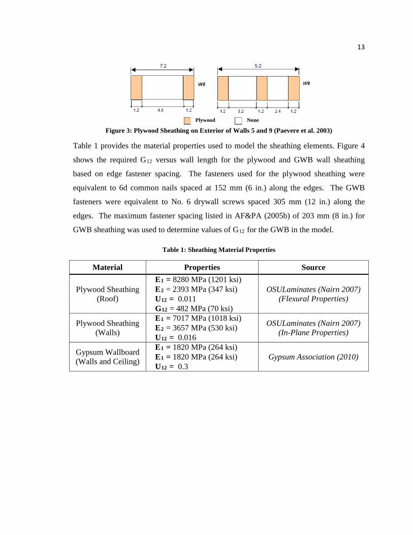
13
Figure 3: Plywood Sheathing on Exterior of Walls 5 and 9 (Paevere et al. 2003)
Table 1 provides the material properties used to model the sheathing elements. Figure 4
shows the required G12 versus wall length for the plywood and GWB wall sheathing
based on edge fastener spacing. The fasteners used for the plywood sheathing were
equivalent to 6d common nails spaced at 152 mm (6 in.) along the edges. The GWB
fasteners were equivalent to No. 6 drywall screws spaced 305 mm (12 in.) along the
edges. The maximum fastener spacing listed in AF&PA (2005b) of 203 mm (8 in.) for
GWB sheathing was used to determine values of G12 for the GWB in the model.
Table 1: Sheathing Material Properties
Material Properties Source
Plywood Sheathing (Roof)
E1 = 8280 MPa (1201 ksi) OSULaminates (Nairn 2007)
(Flexural Properties) E2 = 2393 MPa (347 ksi) U12 = 0.011 G12 = 482 MPa (70 ksi)
Plywood Sheathing (Walls)
E1 = 7017 MPa (1018 ksi) OSULaminates (Nairn 2007) (In-Plane Properties) E2 = 3657 MPa (530 ksi)
U12 = 0.016
Gypsum Wallboard (Walls and Ceiling)
E1 = 1820 MPa (264 ksi) Gypsum Association (2010) E1 = 1820 MPa (264 ksi)
U12 = 0.3
Plywood None

14
Figure 4: G12 vs. Wall Length for Plywood and GWB Wall Sheathing
The walls were anchored with 12.7 mm (0.5 in.) diameter anchor bolts, only (no
hold-downs were used). Vertical and lateral springs used to represent the axial and shear
behavior of the bolt connections were assigned a stiffness of 6.1 kN/mm (35 kip/in) and
16.7 kN/mm (95.5 kip/in), respectively. Stiffness properties were determined from
Seaders (2004) and AF&PA (2005a) as explained in the modeling methods. Each anchor
bolt in the full-scale house was connected to a load cell capable of measuring lateral and
vertical reactions. Reactions at the anchor bolts in the model were validated against
reactions from Paevere et al. (2003) for 15 static load tests consisting of one gravity load
test and 14 lateral, concentrated load tests. Table 2 lists the material densities used to
model the self weight (gravity loads) of the house. A complete list of lateral load cases
can be found in either Paevere (2002) or Pfretzschner (2012).
Table 2: Material Densities used for Building Self-Weight
Material Density kg/m3 (pcf) Source
Framing Members 550 (1.07) Paevere (2002) Plywood 600 (1.16) EWPAA (2009)
GWB 772 (1.50) Gypsum Association (2010)
Load Path Investigations
After the modeling methods were validated, variations of the Paevere et al. (2003)
house were created and used to perform load path investigations for uniform uplift
y = 24.013x - 0.4457
0
50
100
150
200
250
300
0 2 4 6 8 10 12
G12
(MPa
)
Wall Length (m)
9.5 mm Plywood Sheathing
y = -0.7247x + 50.742
0
50
100
150
200
250
300
0 2 4 6 8 10 12
G12
(MPa
)
Wall Length (m)
13 mm GWB Sheathing
15
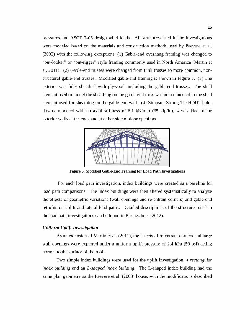
pressures and ASCE 7-05 design wind loads. All structures used in the investigations
were modeled based on the materials and construction methods used by Paevere et al.
(2003) with the following exceptions: (1) Gable-end overhang framing was changed to
“out-looker” or “out-rigger” style framing commonly used in North America (Martin et
al. 2011). (2) Gable-end trusses were changed from Fink trusses to more common, non-
structural gable-end trusses. Modified gable-end framing is shown in Figure 5. (3) The
exterior was fully sheathed with plywood, including the gable-end trusses. The shell
element used to model the sheathing on the gable-end truss was not connected to the shell
element used for sheathing on the gable-end wall. (4) Simpson Strong-Tie HDU2 hold-
downs, modeled with an axial stiffness of 6.1 kN/mm (35 kip/in), were added to the
exterior walls at the ends and at either side of door openings.
Figure 5: Modified Gable-End Framing for Load Path Investigations
For each load path investigation, index buildings were created as a baseline for
load path comparisons. The index buildings were then altered systematically to analyze
the effects of geometric variations (wall openings and re-entrant corners) and gable-end
retrofits on uplift and lateral load paths. Detailed descriptions of the structures used in
the load path investigations can be found in Pfretzschner (2012).
Uniform Uplift Investigation
As an extension of Martin et al. (2011), the effects of re-entrant corners and large
wall openings were explored under a uniform uplift pressure of 2.4 kPa (50 psf) acting
normal to the surface of the roof.
Two simple index buildings were used for the uplift investigation: a rectangular
index building and an L-shaped index building. The L-shaped index building had the
same plan geometry as the Paevere et al. (2003) house; with the modifications described

16
previously, no interior walls, no wall openings and no GWB lining. The rectangular
index building was then created by removing the short leg of the “L” and extending wall
2. Note that the wall designations used by Paevere et al. (2003) (shown in Figure 1) were
maintained throughout both load path investigations. Similar to Martin et al (2011), the
self-weight of the buildings was not included in order to analyze load paths due to uplift
pressures, only. Reactions at the anchor bolts and hold-downs of the L-shaped index
building were compared to the rectangular building to analyze the effects of the re-entrant
corner.
The redistribution of load paths due to large wall openings was also explored in
this investigation. Martin et al. (2011) analyzed the effects of wall openings on uplift
load paths in a simple rectangular building. In the current study, the effects of large, 3.2-
m- (10.5-ft-) long, wall openings in the L-shaped index building were explored. Wall
openings were added to the building one at a time in the following locations, representing
scenarios that were not previously explored by Martin et al. (2011): wall 2 adjacent to the
re-entrant corner, wall 4 opposite the re-entrant corner, wall 9 centered under the gable
end, and wall 9 opposite the re-entrant corner. Due to the configuration of the roof, wall
9 represents both a gable-end wall and a side wall, with trusses running both parallel and
perpendicular to the wall.
Wind Load Investigation
The second load path investigation explored load paths in a more realistic house
with applied ASCE 7-05 design wind loads. Design loads were calculated using the
Main Wind Force Resisting System, MWFRS, method 2 (ASCE 2005). Although ASCE
7-05 MWFRS codified pressures are intended for buildings with regular plan geometry, a
method for adapting the pressures to buildings with re-entrant corners is given in Mehta
and Coulbourne (2010). This methodology was adopted for the current study.
Additional methods of determining design wind loads for irregular buildings are
discussed in Pfretzschner (2012).
Three wind directions were considered with design loads calculated based on
ASCE 7-05 Load Cases 1 and 3 as shown in Figure 6. Load Case 1 includes all
windward, leeward, sidewall and “roof parallel to wind” pressures indicated by ASCE 7-
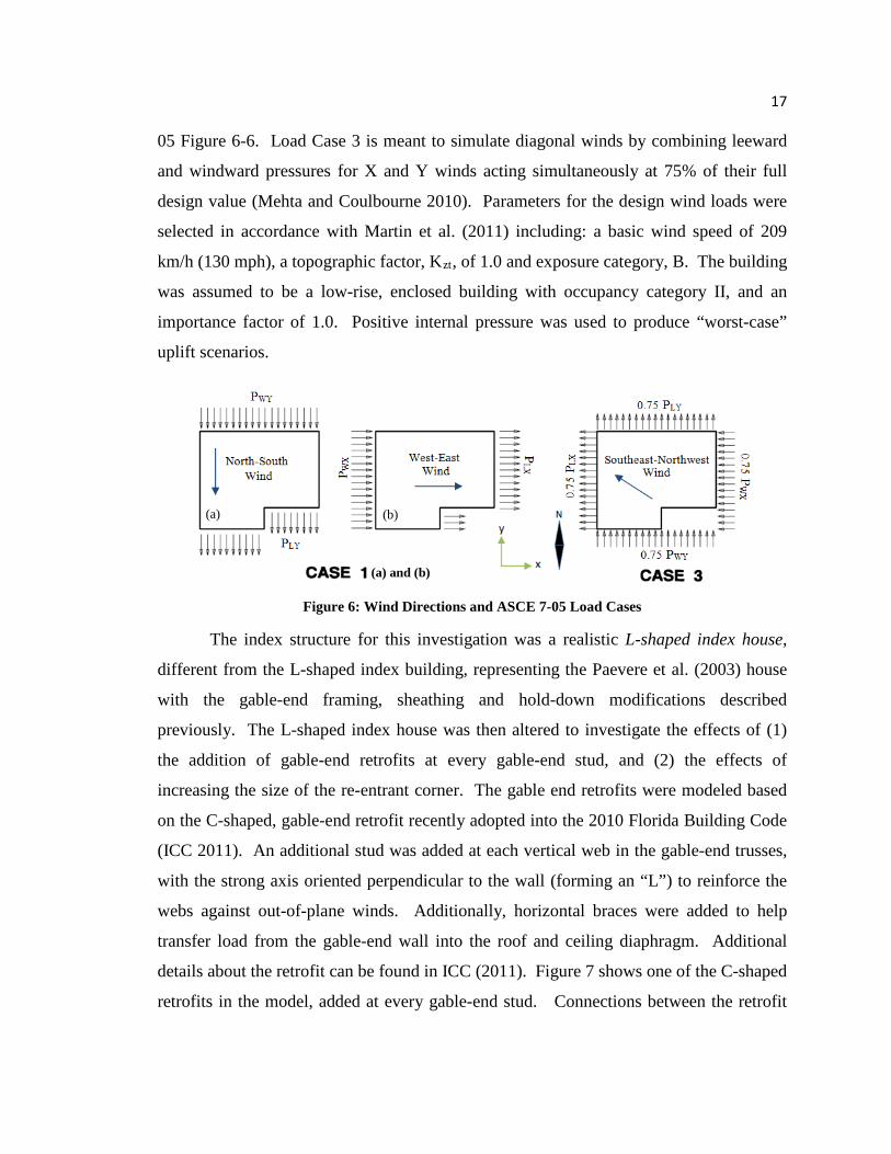
17
05 Figure 6-6. Load Case 3 is meant to simulate diagonal winds by combining leeward
and windward pressures for X and Y winds acting simultaneously at 75% of their full
design value (Mehta and Coulbourne 2010). Parameters for the design wind loads were
selected in accordance with Martin et al. (2011) including: a basic wind speed of 209
km/h (130 mph), a topographic factor, Kzt, of 1.0 and exposure category, B. The building
was assumed to be a low-rise, enclosed building with occupancy category II, and an
importance factor of 1.0. Positive internal pressure was used to produce “worst-case”
uplift scenarios.
Figure 6: Wind Directions and ASCE 7-05 Load Cases
The index structure for this investigation was a realistic L-shaped index house,
different from the L-shaped index building, representing the Paevere et al. (2003) house
with the gable-end framing, sheathing and hold-down modifications described
previously. The L-shaped index house was then altered to investigate the effects of (1)
the addition of gable-end retrofits at every gable-end stud, and (2) the effects of
increasing the size of the re-entrant corner. The gable end retrofits were modeled based
on the C-shaped, gable-end retrofit recently adopted into the 2010 Florida Building Code
(ICC 2011). An additional stud was added at each vertical web in the gable-end trusses,
with the strong axis oriented perpendicular to the wall (forming an “L”) to reinforce the
webs against out-of-plane winds. Additionally, horizontal braces were added to help
transfer load from the gable-end wall into the roof and ceiling diaphragm. Additional
details about the retrofit can be found in ICC (2011). Figure 7 shows one of the C-shaped
retrofits in the model, added at every gable-end stud. Connections between the retrofit
(a) (b)
(a) and (b)

18
studs and horizontal braces were accomplished with steel L-straps and compression
blocks, and modeled as rigid connections.
Figure 7: Example C-Shaped Gable-End Retrofit at Gable-End Stud
The effects of the re-entrant corner were explored by altering the short leg of the
L-shaped index house to create three different sized re-entrant corners: small, medium,
and large. For the small and medium re-entrant corners, the leg was shortened and
lengthened by 2.4 m (7.9 ft) respectively. The large re-entrant corner was created by
extending the leg so that the dimensions of the re-entrant corner had a 1:1 ratio. Wind
loads for the re-entrant corner variations were adjusted accordingly based on the
dimensions of the house.
RESULTS AND DISCUSSION
Model Validation
Sub-Assemblies
Sub-assembly models were used to validate the applicability of previously
described modeling methods in predicting two- and three-dimensional system behavior.
Two-dimensional models of individual trusses validated the use of ideal pinned and rigid
connections between truss chords and webs. Three-dimensional models of roof
assemblies validated the use of the layered shell element for modeling plywood
sheathing. The roof assembly models were capable of predicting load sharing and
relative truss deflection in roofs with variable truss stiffness. Finally, models of two-
19
dimensional shear walls validated methods for incorporating the effects of sheathing
edge-nail spacing, wall openings and wall anchorage on shear wall stiffness. Full details
and results for the sub-assembly validation studies are included in Pfretzschner (2012).
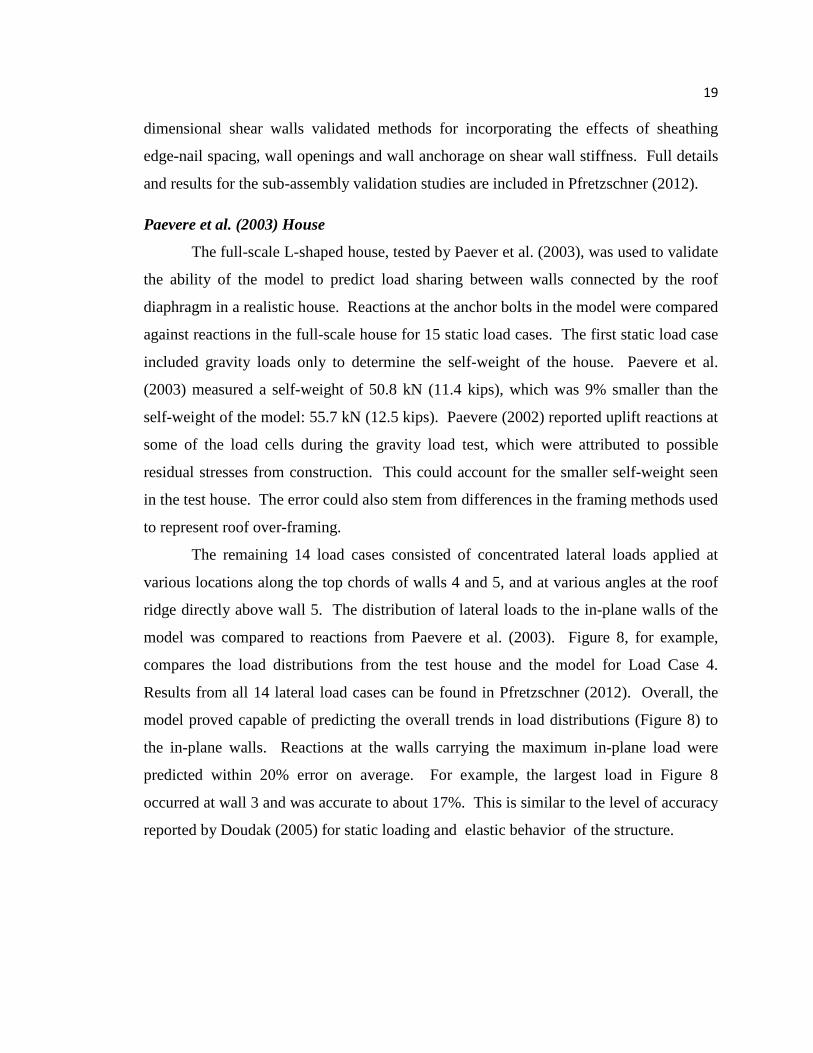
Paevere et al. (2003) House
The full-scale L-shaped house, tested by Paever et al. (2003), was used to validate
the ability of the model to predict load sharing between walls connected by the roof
diaphragm in a realistic house. Reactions at the anchor bolts in the model were compared
against reactions in the full-scale house for 15 static load cases. The first static load case
included gravity loads only to determine the self-weight of the house. Paevere et al.
(2003) measured a self-weight of 50.8 kN (11.4 kips), which was 9% smaller than the
self-weight of the model: 55.7 kN (12.5 kips). Paevere (2002) reported uplift reactions at
some of the load cells during the gravity load test, which were attributed to possible
residual stresses from construction. This could account for the smaller self-weight seen
in the test house. The error could also stem from differences in the framing methods used
to represent roof over-framing.
The remaining 14 load cases consisted of concentrated lateral loads applied at
various locations along the top chords of walls 4 and 5, and at various angles at the roof
ridge directly above wall 5. The distribution of lateral loads to the in-plane walls of the
model was compared to reactions from Paevere et al. (2003). Figure 8, for example,
compares the load distributions from the test house and the model for Load Case 4.
Results from all 14 lateral load cases can be found in Pfretzschner (2012). Overall, the
model proved capable of predicting the overall trends in load distributions (Figure 8) to
the in-plane walls. Reactions at the walls carrying the maximum in-plane load were
predicted within 20% error on average. For example, the largest load in Figure 8
occurred at wall 3 and was accurate to about 17%. This is similar to the level of accuracy
reported by Doudak (2005) for static loading and elastic behavior of the structure.

20
Figure 8: Load Distribution Plot for Paevere et al. (2003) Load Case 4
Uniform Uplift Investigation
The vertical reactions and changes in reaction at the anchor bolts and hold-downs
of the models used in the uplift investigation were recorded and plotted in “bubble” plots.
Each bubble represented an anchor bolt or hold-down while the size of the bubble
represented the magnitude of either the uplift reaction or change in reaction at that
anchorage device. The locations of the hold-downs were designated with an x. Detailed
reaction plots for all model variations can be found in Pfretzschner (2012).
Rectangular vs. L-Shaped Buildings
To analyze the effects of re-entrant corners, the uplift reactions for the rectangular
and L-shaped index buildings were plotted in Figure 9. Uplift reactions in the rectangular
building were symmetrical with a maximum reaction of 11.0 kN (2.5 kips), occurring at
the anchor bolts at the center of the side walls (walls 2 and 4). Since the roof trusses
spanned between the side walls, the majority of the load applied to the roof was directed
into the side walls rather than the gable-end walls. The maximum uplift reaction in the
L-shaped index building, on the other hand, was 14.7 kN (3.3 kips), occurring at the hold-
down directly under the re-entrant corner. In this case, the uplift loads that would have
been transferred to the west side of wall 2 in the rectangular building, were instead
transferred to the garage beam in the L-shaped building (shown in Figure 1b). The
garage beam then directed the loads to the re-entrant corner and wall 9 opposite the re-
entrant corner, causing load concentrations at these locations. Uplift load concentrations
also occurred at anchor bolts under wall 4, directly opposite the re-entrant corner. The
0.0
1.0
2.0
3.0
4.0
5.0
6.0
7.0
8.0
Wall 1 Wall 2 Wall 3 Wall 4
Reac
tion
(kN
)
Paevere et al. (2003)Current Study
NW4
W3
W2W1
4.92 kN

21
flow of loads in the L-shaped index building is illustrated by the arrows in Figure 9.
Note that trusses span perpendicularly from the re-entrant corner to wall 4 at this
location. The load distribution to wall 5, parallel to the trusses, was not affected by the
addition of the re-entrant corner. This suggests that the re-distribution of uplift loads due
to a re-entrant corner is dependent on the orientation of the roof trusses with respect to
the walls. A similar observation was noted by Martin et al. (2011) when investigating the
effects of wall openings. Future research should examine the effects of re-entrant corners
in buildings with different truss orientations.
Figure 9: Uplift Reactions for Rectangular (Left) and L-shaped (Right) Index Buildings
Effects of Wall Openings
Martin et al. (2011) explored the effects of large wall openings placed in the
gable-end walls and side walls of a rectangular building under uniform uplift pressure.
The current study examined openings in an L-shaped building with a re-entrant corner
and trusses oriented in two orthogonal directions. Similar to Martin et al. (2011), the
opening centered under the gable-end portion (North end) of wall 9 caused relatively
localized effects, increasing uplift loads in the side wall portion (South end) of wall 9,
and having negligible effects on walls on the opposite side of the building. The openings
placed in the side walls, on the other hand, had more global effects on uplift reactions
throughout the building. Figure 10 shows the change in uplift reactions due to openings
in the two different side walls: wall 4 (opposite the re-entrant corner) and wall 2 (adjacent
to the re-entrant corner). As expected, uplift loads at the location of the openings were
re-directed through the headers to either side of the doors, causing load concentrations at
Max = 11.0 kN Max = 14.7 kN
N
W1
W2 W2
W4 W4
W5W5W9W9
W7
X
X
X
X
X
X X
X X
X
X = Hold-downs
Trusses Trusses
Garage Beam

22
the hold-downs directly under the door jams. The largest load concentrations were seen
on the side of the opening in wall 2, closest to the re-entrant corner. Uplift reactions at
this point increased by 60 percent over the reactions seen in the building without
openings. Comparatively, the opening in wall 4 caused less than a 30 percent increase in
uplift loads at either side of the opening. The larger load concentration at the opening in
wall 2 was likely due to the uplift load concentrations in wall 2 from the re-entrant corner
itself.
Figure 10: Change in Uplift Reactions (Magnified 4x) due to Openings in Wall 2 (Left) and Wall 4 (Right) – arrows represent load paths
As in Martin et al. (2011), openings placed in the side walls in this investigation
also caused uplift load concentrations in the remaining side walls. Examining the truss
orientation in the building shows that uplift loads at these points of concentration were
clearly transferred from either side of the wall opening by the roof trusses. In the case of
the opening in wall 4, for example, uplift loads were transferred from the east side of the
wall opening, through the north-south trusses, to the opposite side wall (wall 2). Uplift
loads were also transferred from the west side of the opening, through the north-south
trusses to the garage beam shown in Figure 1(b), and redirected through the garage beam
and the east-west trusses to wall 9 (adjacent to wall 4). Similar system behavior was seen
for the opening in wall 2 as shown in Figure 10, and for other side wall openings included
in Pfretzschner (2012). This strongly supports findings from Martin et al. (2011) that the
effects of openings on uplift load distribution are dependent on the relative truss
orientation with respect to the walls. The effects of openings in walls perpendicular to
Max Δ = 3.4 kN27% increase
Max Δ = 6.9 kN60% increase
N
X
X X
X X
XX
X X
X X
X
W1
W2
W4
W5W9
W7W1
W2
W4
W5W9
W7
Increase in Uplift Decrease in Uplift X = Hold-downs
Trusses
Garage Beam Garage Beam

23
the trusses were shared by other walls in the building spanned by the same trusses, while
the effects of openings in walls parallel to the trusses were more isolated.
Finally, Martin et al. (2011) reported that the addition of an opening to any wall
resulted in a decrease in the total load carried by the wall. In the current study, the
opening in wall 2 also caused a decrease in the total load carried by the wall of up to 20
percent. The opening placed in wall 4, however, caused a 0.2 percent increase in the
amount of total uplift load carried by the wall. It is likely that this small increase was due
to the effects of the re-entrant corner.
Wind Load Investigation
Uplift reactions for each of the model variations in the wind load investigation
were also plotted in bubble graphs and included in Pfretzschner (2012). Figure 11 shows
the uplift reactions at the anchor bolts and hold-downs in the L-shaped index house for
each wind load case. In all cases, uplift load concentrations were seen at the hold-downs
located under the corners of the house, as well as on either side of the door openings. In
addition, to determine whether the large uplift reactions at the west gable-end were due to
the geometry of the building or the selected load cases, a fourth load case for east to west
winds was added. This demonstrated that uplift reactions at the east gable end under the
east to west wind loads were of similar magnitude to the reactions at the west gable-end
under west to east wind loads.
Figure 11: Uplift Reactions in L-Shaped Index House
West-East Wind LoadsNorth-South Wind LoadsSoutheast-Northwest Wind LoadsEast-West Wind Loads
X X X X
X
X
X X X
X X
X
X
N
X = Hold-downs
X
W1
W3 W3
W2
W4 W4W5
W5
W9
W9
W7
W6
W8

24
Lateral load distributions to the walls parallel to the wind loads, for each model, were
also plotted (Figure 12) and used to support the findings described below. For the
southeast-northwest load case, lateral load distributions to both the N-S and E-W walls
were plotted. Note that walls 6, 7 and 8 (shown individually in Figure 1) were grouped
together here to simplify data presentation.
Addition of Gable-End Retrofits
Due to the number of gable-end failures seen in the aftermath of hurricanes, the
2010 Florida Building Code recently adopted a C-shaped gable-end retrofit for existing
buildings (ICC 2011). Full-scale tests performed on gable-end sections (comprised of
four Fink trusses and a gable-end wall) by Suksawang and Mirmiran (2009) showed that
the retrofit sufficiently increased the strength of the gable-ends. However, questions
remained about whether load redistribution due to the retrofit could cause additional
torsion within a full building (beyond the original design). To address this question, C-
shaped retrofits were modeled at every gable-end stud within the L-shaped index house
used in this investigation.
The distribution of lateral loads and top plate deflections of the walls were then
analyzed under ASCE 7-05 design wind loads for signs of torsion. For all wind load
cases, the addition of the gable-end retrofits to the L-shaped index house caused
negligible changes in lateral reactions under the walls parallel to the wind loads.
Changes in deflections were equally small, within 0.1 mm (0.004 in), and showed no
signs of additional torsion. These results were based on the three ASCE 7-05 load cases
shown in Figure 6 only. Additionally, alternative retrofits recommended by the 2010
Florida Building Code for buildings with pre-existing obstacles were not explored in this
investigation.
Effects of Re-Entrant Corner Dimensions
Figure 12 shows the lateral load distributions to the walls parallel to the wind
loads and displaced shapes of the exterior wall top-plates for each wind load case. For
north to south (N-S) design wind loads, the displaced shape of the top-chords for each
model variation showed little to no torsion due to the increasing size of the re-entrant

25
corner. As walls 7 and 9 were extended, lateral loads carried by the outer walls running
N-S (walls 5 and 9) were re-distributed to the inner N-S walls 6, 7 and 8. The percent of
N-S loads carried by these central walls increased by 14 percent; while the percent of N-S
loads carried by the outer walls, walls 5 and 9, decreased by 7 and 3 percent, respectively.
In the case of west to east (W-E) wind loads, the displaced shape of the top chords
clearly showed increasing degrees of torsion as the size of the re-entrant corner increased.
Although the relative distribution of these loads to each of the W-E walls changed by less
than 5 percent, increasing the length of the southern end of wall 9 (perpendicular to the
wind) increased the total amount of W-E wind load on the house. As a result, the relative
in-plane deflections of southern walls 1 and 2 as compared to northern walls 3 and 4
increased dramatically. This can be attributed to the fact that walls 1 and 2 were
significantly less stiff than walls 3 and 4, due to the shorter lengths and relatively large
opening to surface-area ratios of walls 1 and 2. This asymmetry in relative stiffness
between the north and south sides of the house caused torsion to occur with increasing
loads in the W-E direction. Wind loads applied diagonally, southeast to northwest (SE-
NW), into the re-entrant corner also caused increasing amounts of torsion as the size of
the re-entrant corner increased. For all load cases, the effects of increasing the size of the
re-entrant corner were dependent on the relative stiffness and location of the walls, as
well as the orientation of the wind loads. Additionally, the displaced shapes of the top
plates in Figure 12 show a combination of torsional behavior and in-plane displacements
characteristic of a semi-rigid diaphragm.

26
Figure 12: Lateral Load Distribution and Top Plate Deflected Shapes for Re-Entrant Corner
Variations
The results of this study imply that balancing the stiffness of the walls along each
of the major axes of the house may reduce torsion due to large re-entrant corners. In an
effort to reduce torsion in the model with the largest re-entrant corner, the stiffnesses of
walls 1 and 2 were increased by assuming realistic changes in the construction of the
walls: (1) blocking was added to the walls, (2) the edge fastener spacing for the GWB
was decreased to 102mm (4 in), (3) the nails used for the plywood were upgraded from
6d to 8d common nails and (4) the edge nail spacing for the plywood was decreased to 51
0%
10%
20%
30%
40%
50%
Wall 9 Wall 6,7,8 Wall 5
% o
f N-S
Rea
ctio
ns
North-South Wind Loads
0%
10%
20%
30%
40%
50%
Wall 1 Wall 2 Wall 3 Wall 4
% o
f E-W
Rea
ctio
ns
West-East Wind Loads
0%
10%
20%
30%
40%
50%
Wall 1 Wall 2 Wall 3 Wall 4
% o
f E-W
Rea
ctio
ns
Southeast-Northwest Wind Loads
N
0%10%20%30%40%50%
Wall 9 Wall 6,7,8 Wall 5
% o
f N-S
Rea
ctio
ns
Southeast-Northwest Wind Loads
Small Re-entrant CornerL-Shaped Index HouseMedium Re-entrant CornerLarge Re-entrant Corner
Top
Pla
te D
efle
cted
Sha
pe W
all 9
Wal
ls
6,7,
8
Wal
l 5
Wall 2
Wall 4
Wall 3
Wall 1

27
mm (2 in). Based on these assumptions, new values of G12 for the GWB and plywood
sheathing on walls 1 and 2 were calculated using the adjustment procedure described in
the modeling methods section. Figure 13 shows the deflected shapes of the original
model and the model with increased stiffnesses in walls 1 and 2 for the W-E and SE-NW
wind loads. In both cases, increasing the stiffnesses of walls on the south side of the
house slightly decreased the amount of torsion seen in the deflected shape of the top
chords.
Figure 13: Displaced Shape of Large Re-Entrant Corner Building with Increased
Stiffness in Walls 1 and 2
CONCLUSIONS
Based on the validation studies, the simplified linear modeling methods created by
Martin et al. (2011), and further developed in this study, were capable of predicting uplift
and lateral load paths in a light-frame, wood residential structure with complex, realistic
plan geometry. This conclusion is strictly for loading conditions within the elastic range
of the structure. The modeling methods used in this study cannot be applied for inelastic
or failure analysis.
Using the validated modeling methods, two different load path investigations were
performed using uniform uplift pressures and ASCE 7-05 design wind loads. The
following conclusions were drawn based on results from the load path investigations:
1. The addition of a re-entrant corner in a low-rise structure, under uniform uplift
pressure, caused load concentrations at the re-entrant corner as well as in either
wall directly opposite the re-entrant corner; depending on the truss orientation.
West-East Wind Loads
Southeast-Northwest Wind Loads
W1 W1
W2 W2

28
2. The addition of wall openings in a low-rise structure under uniform uplift pressure
caused load concentrations on either side of the openings. Uplift loads at these
points of concentration were further distributed to the remaining walls by the roof
trusses. The largest load concentrations occurred when an opening was placed in
a side wall, directly adjacent to the re-entrant corner. Openings in walls parallel
to the trusses had the least effect on uplift reactions in the remaining walls.
3. ASCE 7-05 Main Wind Force Resisting System (MWFRS) design wind loads
caused uplift load concentrations at the hold-downs placed under the door jams
and the corners of the L-shaped house.
4. There was no evidence that the gable-end retrofit adopted by the 2010 Florida
Building Code caused additional torsion in the L-shaped house when loaded with
ASCE 7-05 MWFRS design wind loads.
5. The effects of increasing the size of the re-entrant corner in an L-shaped house,
under ASCE 7-05 MWFRS design wind loads, were dependent on the location
and relative stiffness of the in-plane walls, as well as the assumed direction of the
wind.
ACKNOWLEDGMENTS
Previous research contributions from Kenneth Martin, Dr. Phillip Paevere and Dr.
Bohumil Kasal were greatly appreciated, as well as funding from the Oregon State
University Center for Wood Utilization Research.

29
REFERENCES
AF&PA (2005a). National Design Specification for Wood Construction (NDS). ANSI/AF&PA NDS-2005. Washington, DC.
AF&PA (2005b). Special Design Provisions for Wind and Seismic. ANSI/AF&PA NDS-2005. Washington, DC.
ASCE – American Society of Civil Engineers. (2005). ASCE/SEI 7-05 Minimum Design Loads for Buildings and Other Structures. New York, NY.
Computers and Structures, Inc. (2009). CSI Analysis Reference Manual: For SAP2000, ETABS and SAFE. Berkeley, CA.
Collins, M., Kasal, B., Paevere, P. and Foliente, G. C. (2005). “Three-Dimensional Model of Light Frame Wood Buildings. II: Experimental Investigation and Validation of Analytical Model.” Journal of Structural Engineering, 131(4), 676-683.
Dolan, J.D. and Johnson, A.C. (1996) “Monotonic Tests of Long Shear Walls with Openings.” Virginia Polytechnic Institute and State University Timber Engineering Report TE-1996-001, Blacksburg, VA.
Doudak, G. (2005). “Field Determination and Modeling of Load Paths in Wood Light-Frame Structures.” PhD. Thesis, McGill University, Montreal, Quebec.
EWPPA - Engineered Wood Products Association of Australia (2009). “Structural Plywood and LVL Design Manual.” EWPAA Design Guides, <http://www.ed.ewp.asn.au:85/Library/ document_List.aspx?type=Design> (July 19, 2012).
Gypsum Association (2010). “Gypsum Board Typical Mechanical and Physical Properties.” Gypsum Association (GA 235-10), Hyattsville, MD.
Holmes, J.D., (2001). Wind Loading of Structures. Spon Press, New York, NY.
ICC (2011). Florida Building Code 2010 – Residential. International Code Council, Inc. Country Club Hills, IL.
Kasal, B. (1992) “A Nonlinear Three-Dimensional Finite-Element Model of a Light-Frame Wood Structure.” Ph.D. Diss., Oregon State University, Corvallis, Oregon.
Martin, K. (2010). “Evaluation of System Effects and Structural Load Paths in a Wood Framed Structure.” M.S. Thesis, Oregon State University, Corvallis, OR.
Martin, K.G., Gupta, R., Prevatt, D.O., Datin, P.L., van de Lindt, G.W., (2011). “Modeling System Effects and Structural Load Paths in a Wood-Framed Structure.” Journal of Architectural Engineering. 17, 134-143.

30
Mehta, K.C. and Coulbourne, W.L. (2010). Wind Loads: Guide to the Wind Load Provisions of ASCE 7-05. ASCE Press, Reston, VA.
Nairn, J. (2007). OSULaminates – Java Application for Laminated Theory Analysis, Version 2.1. Available at: < http://www.cof.orst.edu/cof/wse/faculty/Nairn/OSU Laminates.html> (July 31 2012).
Paevere, P. (2002). “Full-Scale Testing, Modeling and Analysis of Light-Frame Structures Under Lateral Loading.” Ph.D. Diss., The University of Melbourne, Victoria, Australia.
Paevere, P., Foliente, A.M., and Kasal, B. (2003). “Load-Sharing and Redistribution in a One-Story Woodframe Building.” Journal of Structural Engineering, 129 (9), 1275-1284.
Patton-Mallory, M., Gutkowski, R.M., and Solstis, L.A. (1984). “Racking Performance of Light-Frame Walls Sheathed on Two Sides.” FPL-448. Forest Products Laboratory, Madison, WI.
Pfretzschner, K.S. (2012). “Practical Modeling for Load Paths in a Realistic, Light-Frame Wood House.” M.S Thesis, Oregon State University, Corvallis, OR.
Phillips, T., Itani, R., and McLean, D. (1993). “Lateral Load Sharing by Diaphragms in Wood-Framed Buildings.” Journal of Structural Engineering, 119(5), 1556-1571.
Prevatt, D.O., Roueche, D.B., van de Lindt, J.W., Pei, S., Dao, T., Coulbourne, W., Graettinger, A.J., Gupta, R., and Grau, D. (2012). “Building Damage Observations and EF Classifications from the Tuscaloosa, AL and Joplin, MO Tornadoes.” Structures Congress 2012, ASCE 2012, 999-1010.
Seaders, P. (2004). “Performance of Partially and Fully Anchored Wood Frame Shear Walls Under Monotonic, Cyclic and Earthquake Loads.” M.S. Thesis, Oregon State University, Corvallis, OR.
Shivarudrappa, R., Nielson, B.G. (2011) “Sensitivity of load distribution in light-framed wood roof systems due to typical modeling parameters.” Journal of Performance of Constructed Facilities, Accepted Manuscript.
Suksawang, N. and Mirmiran, A., “Hurricane Loss Reduction for Housing in Florida: Performance of Gable End Wall Bracing Retrofit for Hurricane Protection, Phase II” Florida International University < http://www.ihrc.fiu.edu/lwer/docs/ Year%209_Section4_GableEndBracing_RCMP08-09.pdf> (July 22, 2012).
van de Lindt, J.W., Graettinger, A., Gupta, R., Skaggs, T., Pryor, S., and Fridley, K.J., (2007). “Performance of Wood-Frame Structures during Hurricane Katrina.” Journal of Performance of Constructed Facilities, 21(2), 108-116.

31
Wolfe, R.W., and McCarthy, M. (1989). “Structural Performance of Light Frame Roof Assemblies – I. Truss Assemblies with High Truss Stiffness Variability” FPL-RP-492. Forest Products Laboratory, Madison, WI.
Wolfe, R.W., Percival, D.H., and Moody, R.C. (1986). “Strength and Stiffness of Light Framed Sloped Trusses.” FPL-RP-471. Forest Products Laboratory, Madison, WI.

32
CONCLUSIONS AND RECOMMENDATIONS
In order to establish effective building codes and retrofit options for houses in
high wind zones, it is important to fully understand the system behavior and propagation
of load paths through these structures. In this study, practical, linear modeling methods
were developed for analyzing load paths in light-frame wood structures. The methods
were validated against full-scale tests and found to be sufficient for predicting load paths
and system behavior when loaded within the elastic range. Once validated, the methods
were used in two load path investigations to analyze the effects of geometric variations
and gable-end retrofits in light-frame wood structures.
The first investigation considered uniform uplift pressures applied to simple
rectangular and L-shaped buildings with no interior walls, no gypsum wall board
(GWB) and no wall openings. Uplift reactions at the anchor bolts and hold-downs in the
two structures were compared to examine the effects of adding a re-entrant corner. In
the L-shaped building, uplift concentrations appeared under the re-entrant corner and
under walls opposite the re-entrant corner. These concentrations occurred in locations
where trusses spanned directly between the re-entrant corner and the opposite walls.
Similar behavior was observed when large openings were systematically added to walls
in the L-shaped building. All openings added to the building caused uplift load
concentrations at either side of the opening. Openings placed in the side-walls caused
additional uplift load concentrations under opposite walls spanned by perpendicular
trusses, while openings placed in gable-end walls (parallel to roof trusses) had little
effect on the remaining walls in the building. This suggested that geometric variations
in a structure can have global effects on uplift loads throughout the structure depending
on the orientation of the roof trusses. Effects of large openings can be contained to local
areas of the building by placing them in gable-end walls, parallel to the trusses.
The second load path investigation evaluated lateral and uplift load paths in a
realistic L-shaped house (with interior walls, GWB and realistic door and window
openings) under ASCE 7-05 MWFRS design wind loads. During the investigation, the
house was modified to determine the effects of gable-end retrofits and varying re-entrant
33
corner dimensions on the distribution of loads. Uplift reactions at anchor bolts and hold-
downs in the original L-shaped house showed load concentrations at either side of door
openings and at the corners of the structure (including the re-entrant corner). Gable-end
retrofits recommended by the 2010 Florida building Code were added to investigate
effects on lateral load distributions (ICC 2011). Although the retrofits have proved
effective in previous full-scale tests, questions remained about the possible effects on
load paths and torsion within a full building. Lateral load distributions and displaced
shapes of the retrofitted, L-shaped house in this study showed no signs of additional
torsion due to the gable-end retrofits. The effects of re-entrant corner dimensions were
analyzed by altering the length of one leg of the “L” in the original house. Lateral load
distributions and displaced shapes of the models with various re-entrant corner
dimensions showed that the effects of large re-entrant corners were dependent on the
relative stiffness of the walls and the direction of loading. Balancing the stiffness of
walls on either side of the building may help reduce the amount of torsion caused by the
re-entrant corner.
Results from this study were limited to an L-shaped building. Future research
should consider buildings with T, Y, X and U-shaped plan geometries, as well as
alternate truss orientations. Furthermore, additional emphasis should be placed on using
models to develop and verify retrofitting options for residential structures. This task
may require a combination of the simplified modeling methods described in the current
study and more detailed models of sub-assemblies. Finally, there was a considerable
amount of debate concerning methods for calculating wind loads on buildings with
irregular geometry and very little published information on the subject. Combining full
building models with wind tunnel tests on scaled structures could help to verify current
methods for calculating wind loads on structures with re-entrant corners.

34
BIBLIOGRAPHY
AF&PA (2005a). National Design Specification for Wood Construction (NDS). ANSI/AF&PA NDS-2005. Washington, DC.
AF&PA (2005b). Special Design Provisions for Wind and Seismic. ANSI/AF&PA NDS-2005. Washington, DC.
Amini, M.O. (2012). “Determination of Rational Tornado Design Wind Speed for Residential Woodframe Structures.” M.S. Thesis, University of Alabama, Tuscaloosa, AL.
APA – The Engineered Wood Association (2008). Panel Design Specification. The Engineered Wood Association. Tacoma, Washington.
ASCE – American Society of Civil Engineers. (2005). ASCE/SEI 7-05 Minimum Design Loads for Buildings and Other Structures. ASCE, New York, NY.
Collins, M., Kasal, B., Paevere, P. and Foliente, G. C. (2005a). “Three-Dimensional Model of Light Frame Wood Buildings. II: Experimental Investigation and Validation of Analytical Model.” ASCE Journal of Structural Engineering, 131(4), 676-683.
Collins, M., Kasal, B., Paevere, P. and Foliente, G. C. (2005b). “Three-Dimensional Model of Light Frame Wood Buildings. I: Model Description.” ASCE Journal of Structural Engineering, 131(4), 684-692.
Computers and Structures, Inc. (2009). CSI Analysis Reference Manual: For SAP2000, ETABS and SAFE. Berkeley, CA.
Cramer, S. M., and Wolfe, R. W. (1989). “Load-Distribution Model for Light-Frame Wood Roof Assemblies.” ASCE Journal of Structural Engineering, 115(10), 2603-2615.
Cramer, S.M., Drozdek, J.M., and Wolfe, R.W. (2000) “Load Sharing Effects in Light-Frame Wood-Truss Assemblies” ASCE Journal of Structural Engineering, 115(10), 2602-2616.
Dolan, J.D. and Johnson, A.C. (1996) “Monotonic Tests of Long Shear Walls with Openings.” Virginia Polytechnic Institute and State University Timber Engineering Report TE-1996-001.
Doudak, G. (2005). “Field Determination and Modeling of Load Paths in Wood Light-Frame Structures.” PhD. Thesis, McGill University, Montreal, Quebec.

35
Doudak, G., McClure, G., and Smith, I. (2012). “Experimental Evaluation of Load Paths in Light-Light Frame Wood Structure.” ASCE Journal of Structural Engineering., 138(2), 258-265.
Dung, D. (1999). “A practical approach to analyze the system effects of metal-plate-connected wood truss assembly.” MS thesis, Oregon State University, Corvallis, Oregon.
EWPPA - Engineered Wood Products Association of Australia (2009). “Structural Plywood and LVL Design Manual.” EWPAA Design Guides, <http://www.ed.ewp.asn.au:85/Library/ document_List.aspx?type=Design> (July 19, 2012).
Fanella, D.A. (2008). Structural Load Determination Under 2006 IBC and ASCE/WEI 7-05. International Code Council, Springfield, IL.
Gupta, R. (2005). “System Behaviour of Wood Truss Assemblies.” Prog. Strct. Engng. Mater., 7: 183-193.
Gupta, R., and Limkatanyoo, P. (2008). “Practical Approach to Designing Wood Roof Truss Assemblies.” Practice Periodical on Structural Design and Construction, 13(3), 183-193.
Gupta, R., Miller, T. H., and Dung, D. (2004). “Practical solution to wood truss assembly design problems.” Practice Periodical on Structural Design and Construction, 9(1), 54-60.
Gypsum Association (2010) “Gypsum Board Typical Mechanical and Physical Properties” Gypsum Associaiton (GA 235-10)
Holmes, J.D., (2001). Wind Loading of Structures. Spon Press, New York, NY.
ICC (2011). Florida Building Code 2010 – Residential. International Code Council, Inc. Country Club Hills, IL.
Kasal, B. (1992) “A Nonlinear Three-Dimensional Finite-Element Model of a Light-Frame Wood Structure.” Ph.D. Diss., Oregon State University, Corvallis, Oregon.
Kasal, B., Collins, M. S., Paevere, P. and Foliente, G. C. (2004). “Design Models of Light Frame Wood Buildings under Lateral Loads.” ASCE Journal of Structural Engineering, 130(8), 1263-1271.
Kasal, B., and Leichti, R. J. (1992). “Nonlinear Finite-Element Model for Light-Frame Stud Walls,” ASCE Journal of Structural Engineering, 118 (11), 3122-3135.
Kasal, B., Leichti, R. J. and Itani, R. (1994). “Nonlinear Finite Element Model of Complete Light-Frame Structures.” ASCE Journal of Structural Engineering, 120(1), 100-119.

36
LaFave, K. and Itani, R. Y. (1992). “Comprehensive Load Distribution Model for Wood Truss Roof Assemblies.” Wood and Fiber Science, 24(1), 79-88.
Langlois, J.D. (2002). “Effects of Reference Displacement and Damage Accumulation in Wood Shear Walls Subjected to the CUREE Protocol.” M.S. Thesis, Oregon State University, Corvallis, OR.
Langlois, J., Gupta, R., and Miller, T.H. (2004). “Effects of reference displacement and damage accumulation in wood shear walls.” ASCE Journal of Structural Engineering, 130(3), 470-479.
Lebeda, D.J. (2002). “Behavior of Wood Shear Walls with Misplaced Holdowns.” M.S. Thesis, Oregon State University, Corvallis, Oregon.
Lebeda, D., Gupta, R., Rosowsky, D. and Dolan, J.D. (2005). “The effect of hold-down misplacement on the strength and stiffness of wood shear walls.” Practice Periodical on Structural Design and Construction, 10(2), 79-87.
Li, Z. (1996). “A Practical Approach to Model the Behavior of a Metal-Plate-Connected Wood Truss System.” M.S. thesis, Oregon State University, Corvallis, Oregon.
Li, Z., Gypta, R., and Miller, T.H. (1998). “Practical approach to modeling of wood truss roof assemblies.” Practice Periodical on Structural Design and Construction, 3(3): 119-124.
Limkatanyoo, P. (2003). “System Behavior of Three-Dimensional Wood Truss Assemblies.” M.S. Thesis, Oregon State University, Corvallis, Oregon.
Martin, K. (2010). “Evaluation of System Effects and Structural Load Paths in a Wood Framed Structure.” M.S. Thesis, Oregon State University, Corvallis, OR.
Martin, K.G., Gupta, R., Prevatt, D.O., Datin, P.L., van de Lindt, G.W., (2011). “Modeling System Effects and Structural Load Paths in a Wood-Framed Structure.” ASCE Journal of Architectural Engineering. 17, Special Issue: Residential Construction, 134-143.
Mehta, K.C. and Coulbourne, W.L. (2010). Wind Loads: Guide to the Wind Load Provisions of ASCE 7-05. American Society of Civil Engineers - ASCE Press, Reston, VA.
Mensah A.F., et al. (2010) “Database-assisted design methodology to predict wind-induced structural behavior of a light-framed wood building.” Engineering Structures (2010), doi: 10.1016/j.engstruct2010.11.028.
Mtenga, P. (1991). “Reliability Performance of Light-Frame Wood Roof Systems.” PhD. Thesis, University of Wisconsin-Madison, Madison, Wisconsin.

37
Nairn, J. (2007). OSULaminates – Java Application for Laminated Theory Analysis, Version 2.1. Available at: <http://www.cof.orst.edu/cof/wse/faculty/Nairn /Software.htm>. Oregon State University, Corvallis, Oregon.
Paevere, P. (2002). “Full-Scale Testing, Modeling and Analysis of Light-Frame Structures Under Lateral Loading.” Ph.D. Diss., The University of Melbourne, Victoria, Australia.
Paevere, P., Foliente, A.M., Kasal, B. (2003). “Load-Sharing and Redistribution in a One-Story Woodframe Building.” ASCE Journal of Structural Engineering, 129 (9), 1275-1284.
Patton-Mallory, M., Gutkowski, R.M., Solstis, L.A. (1984). “Racking Performance of Light-Frame Walls Sheathed on Two Sides.” FPL-448. Forest Products Laboratory, Madison, WI.
Phillips, T. L. 1990. "Load Sharing Characteristics of Three-Dimensional Wood Diaphragms." M.S. Thesis, Washington State University, Pullman, WA.
Phillips, T., Itani, R., and McLean, D. (1993). “Lateral Load Sharing by Diaphragms in Wood-Framed Buildings.” ASCE Journal of Structural Engineering, 119(5), 1556-1571.
Prevatt, D.O., Datin, P.L. and Mensah, A. (2009) “Performance Based Wind Engineering (PBWE): Interaction of Hurricanes with Residential Structures” Proc. 2009 NSF Engineering Research and Innovation Conference, National Science Foundation, Honolulu, HI.
Prevatt, D.O., Roueche, D.B., van de Lindt, J.W., Pei, S., Dao, T., Coulbourne, W., Graettinger, A.J., Gupta, R., Grau, D., (2012a). “Building Damage Observations and EF Classifications from the Tuscaloosa, AL and Joplin, MO Tornadoes.” Structures Congress 2012, ASCE 2012, 999-1010.
Prevatt, D.O., Beata, P.A., Roueche, D.B., Consolazio, G.R., and Datin, P.L. (2012b) “Database-assisted Design and Finite Element Analysis of Residential Light-Framed Wood Structures.” 1st International Conference on Performance Based and Life Cycle Structural Engineering, Hong Kong, China.
Rocha, D., Eamon, C.D., Murphy, J.F. (2010). “Reliability anaylsis of roof sheathing panels exposed to a hurricane wind” Elsevier Journal of Structural Safety, 33(2011), 74-81.
Seaders, P. (2004). “Performance of Partially and Fully Anchored Wood Frame Shear Walls Under Monotonic, Cyclic and Earthquake Loads.” M.S. Thesis, Oregon State University, Corvallis, OR.
38
Shanmugam, B., Nielson, B.G., Prevatt, D.O. (2008). “Probabilistic descriptions of in-situ roof to top plate connections in light frame wood structures.” ASCE Structures Congress 2008: Crossing Borders.
Shivarudrappa, R., Nielson, B.G. (2011) “Sensitivity of load distribution in light-framed wood roof systems due to typical modeling parameters.” Journal of Performance of Constructed Facilities, Accepted Manuscript.
Simpson Strong-Tie (2012a) “Discontinued Products.” Simpson Strong-Tie, <http://strongtie .com/obsolete.html> (July 7, 2012).
Simpson Strong-Tie (2012b) “LTT/HTT Tension Ties.” Simpson Strong-Tie, <http://strongtie .com/products/connectors/LTT-HTT.asp> (July 7, 2012)
Sinha, A. (2007). “Strain Distribution in OSB and GWB in Wood Frame Shear Walls.” M.S. Thesis, Oregon State University, Corvallis, OR.
Songlai, C., Chengmou, F., and Jinglong, P. (2010). “Experimental Study on Full-Scale Light-Frame Wood House under Lateral Load.” ASCE Journal of Structural Engineering, 136(7), 805-812.
Suksawang, N., Mirmiran, A., “Hurricane Loss Reduction for Housing in Florida: Performance of Gable End Wall Bracing Retrofit for Hurricane Protection, Phase II” Florida International University < http://www.ihrc.fiu.edu/lwer/docs/ Year%209_Section4_GableEndBracing_RCMP08-09.pdf> (July 22, 2012).
Taly, N., “Loads and Load Paths in Buildings: Principles of Structural Design,” International Code Council, ICC Publishing, Country Club Hills, IL.
van de Lindt, J.W., Graettinger, A., Gupta, R., Skaggs, T., Pryor, S., and Fridley, K.J., (2007). “Performance of Wood-Frame Structures during Hurricane Katrina.” Journal of Performance of Constructed Facilities, 21(2), 108-116.
Wolfe, R.W., and LaBissoniere, T. (1991). “Structural Performance of Light Frame Roof Assemblies – II. Conventional Truss Assemblies” FPL-RP-499. Forest Products Laboratory, Madison, WI.
Wolfe, R.W., and McCarthy, M. (1989). “Structural Performance of Light Frame Roof Assemblies – I. Truss Assemblies with High Truss Stiffness Variability” FPL-RP-492. Forest Products Laboratory, Madison, WI.
Wolfe, R.W., Percival, D.H., and Moody, R.C. (1986). “Strength and Stiffness of Light Framed Sloped Trusses.” FPL-RP-471. Forest Products Laboratory, Madison, WI.

39
APPENDIX A
EXTENDED LITERATURE REVIEW
System Behavior and Modeling
Full Building
Light-frame wood structures are highly indeterminate structural systems
composed of vertical (shear walls) and horizontal (roof and floor) subassemblies, joined
by inter-component connections (including nails, screws and other mechanical
connectors). Lateral and vertical external forces are transferred through out-of-plane
walls, to the horizontal roof and floor diaphragms, to the shear walls and finally into the
foundation. Consequently, load paths through the structure as a whole are dependent on
both the behavior of the individual subassemblies, as well as the interaction between
subassemblies. Current design methods often consider each subassembly separately,
which can possibly lead to unsafe or inefficient designs. In order to accurately predict
load paths, the full system must be considered.
Testing and Behavior
Due to the high costs associated with the construction and testing of complete
structures, as well as the limited number of facilities capable of performing such tests,
very few full-scale tests on light-frame wood structures have been performed. Until
recently, the majority of full- scale testing has focused on individual roof and wall
assemblies (discussed in later sections of this review).
Phillips et al. (1993) performed full-scale static tests on a single-story, light-frame
wood structure at Washington State University. The structure was rectangular in plan,
with two interior walls and door and window openings. Doors, windows and other
architectural finishes were not installed in the building. Sheathing edge nail spacing was
varied for each wall to create variable wall stiffness. The structure was cyclically loaded
in three stages with hydraulic cylinders, and reaction forces under each shear wall were
measured. The objective of the project was to provide data for an analytical model

40
created by Kasal (1992). Therefore, materials and subassemblies were also tested during
construction in order to assemble adequate data for model validation.
Similarly, Paevere et al. (2003) performed full-scale testing on a North American
style L-shaped light-frame wood house at the Commonwealth Scientific & Industrial
Research Organization (CSIRO) Division of Building, Construction and Engineering in
Melbourne, Australia. Plans and specifications for the test structure were developed by
the National Association of Home Builders (NAHB) Research Center, CSIRO, and North
Carolina State University. As in Phillips (1990), the objective was to provide data for
finite element modeling. Architectural finishes were not included in the test structure,
and various tests were performed on the materials and subassemblies during construction.
The full structure was tested in multiple stages including: elastic tests, non-destructive
dynamic tests and destructive tests. Reaction forces were measured by tri-axial load cells
spaced evenly under all walls, and deflections were also measured at various locations.
This structure was used to validate multiple finite element models that are discussed
further in the next section.
Doudak (2005) and Doudak et al. (2012) established a real time monitoring
program on a wood-frame house located on the campus of the University of New
Brunswick in Canada. The structure has a simple rectangular plan and rests on a series of
load cells around its perimeter. The structure was first tested under a series of static point
loads to validate an analytical model developed by Doudak (2005) as discussed in the
next section. The structure was then instrumented for continuous in-situ monitoring to
measure the structure’s response to actual dynamic and static environmental loads.
Among the observations noted by Phillips et al. (1993), Paevere et al. (2003) and
Doudak et al. (2012), the following behavioral aspects of structures are important to the
research at hand:
1. Despite its overall flexible behavior, the roof diaphragm acts relatively rigid when
compared to the shear walls (Phillips et al. 1993, Paevere et al. 2003 and Doudak
et al. 2012).
2. In-plane shear walls can transfer approximately 20 to 80 percent of their load to
the rest of the structure when loaded individually (Paevere et al. 2003 and Doudak

41
et al. 2012). Additionally, the amount of load sharing is dependent on the relative
location and stiffness of the loaded wall compared to the surrounding walls in the
structure (Phillips et al. 1993 and Paevere et al. 2003).
3. The transverse shear walls can carry approximately 5 to 25 percent of the load
depending on the type of loading (Phillips et al. 1993 and Paevere et al. 2003).
This percentage decreased with increasing magnitude of applied load (Phillips et
al. 1993).
Finally, Songlai et al. (2010) performed full-scale tests on a single-story, L-
shaped, light-frame wood house under uniform lateral loads. The house was constructed
with a floor diaphragm rather than a roof diaphragm, representing the first story of a
structure. Results of the study showed that gypsum sheathing had significant effects on
the strength and stiffness of shear walls (Songlai et al. 2010). Additionally, the floor
diaphragm acted as a semi-rigid diaphragm in transferring lateral loads to the shear walls
(Songlai et al. 2010).
Analytical Modeling
As a result of the intrinsic level of complexity of light-frame wood structures, a
number of simplifying assumptions must be made to develop a practical analytical model.
The most debated assumptions for system models are those concerning the behavior of
inter-component connections, which are semi-rigid and behave non-linearly. Additional
assumptions include representation of subassemblies, which can either be modeled using
individual construction materials or idealized to various levels based on results from full-
scale tests. Material properties can also be modeled based on recommended values from
engineering design specifications, or can be entered as actual values given sufficient
testing data.
Kasal (1992) used ANSYS finite-element software to develop an analytical model
of the structure tested by Phillips (1990). The roof and floor were modeled as relatively
rigid, linear “superelements” incorporating only the degrees of freedom along the
boundaries of the element. Individual trusses and joists were not included. The walls
were modeled as simplified nonlinear systems based on full-scale tests as discussed

42
further in the shear wall section of this review. Finally, inter-component connections
were modeled using one-dimensional, nonlinear springs. Nonlinear spring properties
were based on load-displacement relationships developed through experimental tests
performed at Oregon State University. The model was accurate in predicting boundary
reaction forces and deformations, but was relatively inaccurate when small loads were
applied. Similar methods were also employed by Collins et al. (2005a,b) in developing
ANSYS models of the more realistic CSIRO house from Paevere et al. (2003).
The models discussed thus far present a few limitations. For example, the level of
simplification of the shear wall assemblies in the three-dimensional model requires that
the boundary forces be taken from the original model and applied to separate, more
detailed models of the individual walls in order to determine individual nail forces.
Doudak (2005) addressed this problem in a model of the New Brunswick House and the
Paevere et al. (2003) house created in SAP2000. Sheathing nail connections were
individually detailed within each wall using spring elements. The finite element model
was able to accurately predict the three-dimensional behavior of the building under
various loads, the interactions between the roof and walls, as well as the interactions
within the individual walls without the need for additional models. Unfortunately, the
amount of time that was required for this level of detailing proved impractical for use in
modeling for industry design.
Another limitation to these models is the element used to represent the roof,
which may not be applicable to more complex structures. Like Kasal (1992) and Collins
(2005a,b), Doudak (2005) also modeled the roof as a single linear element, neglecting the
individual trusses. The load distribution in roof assemblies, however, is dependent on the
relative stiffness of individual trusses. In roofs with complex geometries, different sizes
and types of trusses lead to large variations in stiffness that would not be accounted for in
the simplified models described above.
Martin (2010) incorporated individual trusses into an analytical model of a simple
rectangular building. Similar to Kasal (1992), individual nails in the shear walls were not
detailed. Instead, the directional shear modulus in the sheathing was adjusted to
incorporate the effects of nail spacing as explained in the shear wall section of this report.

43
The model was simplified even further than in earlier models by assuming linear
behavior in the inter-component connections based on properties provided by the
connection manufacturer. Martin (2010) validated the full model against wind tunnel
experiments performed on a scaled version of the building at the University of Florida
with good results. It is important to note that unlike the previous models, the methods
used by Martin (2010) relied on properties found readily available in industry
specifications rather than properties determined from tests performed on materials and
connections for the particular building being modeled.
The objective of the current project is to develop a practical means for exploring
load paths through light-frame wood buildings with realistic, complex geometry. For this
purpose, the methods used by Martin (2010) are ideal. The modeling of individual roof
trusses allows for accurate representations of complex roofs. Additionally, the model
relies on properties that are easily found in specifications rather than properties measured
from experimental tests. This is ideal for industry since buildings are designed well
before construction begins. While Martin (2010) and other previous studies modeled
structures with simple plans, the current model accounts for the growing geometric
complexity in actual residential structures.
Roof Assemblies
Light-framed wood roof assemblies typically consist of a series of trusses spaced
approximately 0.6 m (2 ft) on center and sheathed with plywood or OSB to produce a
system capable of complex load transfer mechanisms. Conventionally, trusses are
designed individually by incorporating a tributary area approach for calculating design
loads. Under this methodology, system behavior within the full assembly is accounted
for by a repetitive system factor. Although roofs designed in this manner have performed
favorably in the past, the increasingly complicated geometries of modern roof systems
over the past few decades have created a need for a better understanding of load transfer
through complex truss assemblies (Gupta 2005).

44
Testing and Behavior
In the 1980’s, the Forest Products Laboratory in Wisconsin began a series of full-
scale tests on light-frame wood truss assemblies to compile a database of information on
system behavior for use in developing structural models. Wolfe et al. (1986) began the
series by testing 42 full-sized Fink trusses using 38 x 89 mm (1.5 x 3.5 in), referred to as
nominal 2x4, wood framing members with variable stiffness properties and metal plate
connections. Wolfe and McCarthy (1989) and Wolfe and LaBissoniere (1991) continued
the study by testing four 9-truss roof assemblies: two with highly variable truss stiffness
properties, and two with more uniform, conventional construction. Based on the roof
assembly tests, Wolfe and McCarthy (1989) and Wolfe and LaBissoniere (1991)
concluded that:
1. Individual trusses and trusses within the assembly behaved approximately
linearly when loaded up to twice their design loads.
2. Deflections of the individual trusses within the assembly were 50% lower
than trusses outside the assembly under similar loading.
3. Composite action between the sheathing and the top chords effectively
increased the stiffness of the top chords by up to 20%.
4. 40 – 70% of loads applied to trusses within the assembly were transferred
through the sheathing to adjacent trusses.
5. Stiffer trusses tended to attract and carry a larger percentage of the applied
loads.
6. Assemblies acted as parallel systems, in which loads are carried in proportion to
truss stiffness rather than being uniformly distributed across tributary areas as
commonly assumed by conventional design practices.
Lafave and Itani (1992) also performed tests on 9-truss gable roof assemblies
constructed using conventional construction and tested on pinned and roller supports.
The end trusses were placed on wooden blocks to simulate stiffer gable end trusses that
were not considered in previous studies. The results of these tests showed that the stiffer
gable end trusses attracted a large amount of the load away from adjacent trusses up to
two trusses away from the ends.

45
Shanmugam et al. (2008) performed in-situ tests on existing roof to wall toe-nail
connections to analyze differences between as-built connections and laboratory tests.
Results showed that the average capacity of the as-built connections was lower than
previous laboratory tests, with a higher variability. Additionally, there was a strong
correlation between the uplift capacity and stiffness of the connections.
Analytical Modeling
Using information collected by the Forest Products Laboratory, several different
analytical models were developed by various researchers. Cramer and Wolfe (1989) used
a matrix analysis program called ROOFSYS to model four nine-truss roof assemblies
(two with high degrees of stiffness variation) similar to those tested by the Forest
Products Laboratory. Individual trusses were modeled with simple pinned connections
throughout. Sheathing was modeled using continuous beam elements on either side of
the truss ridge to incorporate the effects of load transfer. Composite effects from the
addition of roof sheathing were modeled by adjusting the moment of inertia of the top
chords for each truss. The model portrayed similar load sharing behavior as the full-scale
assembly tests, showing that approximately 50% of loads applied to a single truss within
the assembly were transferred to adjacent trusses. Cramer and Wolfe (1989) recognized
that although the model performed well for the nine-truss assemblies that were studied, it
would be difficult and time consuming to apply to more complex roof systems.
LaFave and Itani (1992) developed and validated a comprehensive finite element
model of a simple gable roof assembly. The finite element model included more realistic
semi-rigid spring elements for the metal plate connections, and successfully predicted the
load distributions seen in the actual assembly. The model validated that the stiffer gable
end trusses attracted load away from adjacent trusses up to two trusses away from the
ends. While this model attempted to simulate a more realistic gable roof, however, its
applicability to more complex geometries was still questionable.
Mtenga (1991) and Cramer et al. (2000) used computer modeling to derive system
(or load sharing) factors for application to roof design. Mtenga (1991) developed a 9-
truss, simple gable roof model in a non-linear modeling program called NARSYS.

46
Composite and load sharing effects were included in the same manner as Cramer and
Wolfe (1989), and non-linear, semi-rigid connections were used to incorporate the
behavior of plate connections. Mtenga (1991) found that the repetitive system factor of
1.15, recommended by the National Design Specification (AF&PA 2005a), was relatively
conservative. A sensitivity study was also performed, demonstrating that sheathing
thickness had little effect on the system factors. Changes in configuration or slope of the
assembly, on the other hand, could affect the factors dramatically.
Cramer et al. (2000) used a non-linear modeling program called SAWFTR.
Unlike the model by Mtenga (1991), Cramer et al. (2000) modeled six different truss
assemblies and a joist floor assembly. Composite action was neglected, and only load
sharing behavior was explored. Cramer et al. (2000) agreed that the NDS repetitive
system factor of 1.15 was conservative for floor assemblies, and some roof trusses,
however, the roof truss system factors ranged from 1.06 to 1.24, depending largely on the
stiffness and strength of the truss in question, and those of adjacent trusses.
With the development of commercialized software for modeling, researchers
including Li (1996), Dung (1999) and Limkatanyoo (2003) began creating models for
more practical applications. Li (1996) modeled simple gable style truss assemblies
similar to those tested by the Forest Products Laboratory using a commercial program
called ETABS. Linear, semi-rigid connections were modeled at the heels of the trusses
only, while all other joints were modeled with simple rigid or pinned connections.
Composite action was incorporated by adjusting the moment of inertia of the top chords,
and sheathing was modeled using the program’s beam elements, which were assigned the
same thickness and stiffness properties as structural grade plywood. Sheathing was
connected to the top chords using rigid connections where sheathing joints were flush,
and pinned connections where gaps were present. The model accurately depicted the
three-dimensional system behavior of tests performed in the literature, and demonstrated
that simplified joint connections could still provide accurate results.
Dung (1999) and Limkatanyoo (2003) took commercial program modeling one
step further, by incorporating more complex, realistic geometries. Both studies were
performed in SAP2000 and validated against the Forest Products Laboratory full- scale

47
tests. Dung (1999) modeled an L-shaped hip roof assembly, as well as a T-shaped
assembly with two gable end trusses. Individual trusses were simulated with semi-rigid
connections at heal and peak joints in accordance with material properties provided by
truss-plate manufacturers. All other joints were modeled as either rigid or pinned as in Li
(1996). Roof sheathing was also modeled with beam elements having the same
thickness, stiffness, and width of actual plywood. Gaps between sheathing elements and
composite action were not considered based on sensitivity studies performed by previous
researchers. Limkatanyoo (2003) simplified the modeling methods of Dung (1999) even
further and validated that the use of rigid connections to represent plate connections
produced reasonably accurate results compared to semi-rigid modeling. This more
practical approach was used to model and compare assemblies with the same geometries
used by Dung (1999) in addition to creating and exploring a complex hip roof system.
Dung (1999) and Limkatanyoo (2003) determined combined stress indices
(CSI’s) for trusses within the complex assemblies, and compared them to CSI values
recommended by truss manufacturers. While most CSI values determined within the
assemblies were smaller than recommended values due to system effects; a few trusses
surpassed a CSI of 1.0 suggesting potentially unsafe conditions. Such conditions
occurred where trusses with more flexible supports (trusses supported by other trusses)
transferred significantly large loads to supporting and neighboring trusses. Most
surprisingly, Limkatanyoo (2003) noted that compression within bottom chords was
observed in some areas of the complex hip roof system. Conventional design assumes
that the bottom chords of trusses experience tension forces, and does not consider
compression.
Limkatanyoo (2003) highlighted an issue with using beam elements for sheathing,
as the behavior was highly dependent on the orientation of the elements. This issue was
addressed by Martin (2010), who substituted the beam elements with SAP2000’s thick
shell element. This substitution was applied to the same pinned and rigid modeling
techniques employed by Limkatanyoo (2003) in order to model the gable roof assembly
tested by Wolfe and McCarthy (1989). The model showed that the use of the shell
element surpassed the beam elements as a representation in sheathing in both practicality
48
as well as accuracy. The current project uses the same practical modeling techniques as
Martin (2010), but applies them to a roof assembly with a more complex geometry,
similar to Limkatanyoo (2003).
Rocha et al. (2010) analyzed the reliability of roof sheathing panels under realistic
hurricane wind loads using detailed modeling methods. Individual sheets of sheathing
were depicted using plate elements, disconnected along the edges to form gaps. Frame
elements were used to represent individual sheathing nail connections. When compared
to more simplified models, the detailed model showed significant differences concerning
the reliability of sheathing panels, suggesting that detailed models should be used for
analysis beyond the elastic range of a structure.
Shear Walls
Shear walls serve as one of the main force resisting systems in structures exposed
to wind, seismic and other lateral loads. Until recently, analysis and design for these
substructures was simple and straight forward. With the growing complexity of geometry
and the increasing number and size of openings for doors and windows in residential
structures, however, traditional methods of analysis are no longer viable (Doudak 2005).
Testing and Behavior
Doudak (2005) performed full-scale tests on seven different 2.4 m x 2.4 m (8 ft x
8 ft) shear wall configurations, containing various openings and tie-down patterns. The
walls were constructed using conventional Canadian construction methods and tested
under a combination of gravity and racking loads. Doudak (2005) observed the following
behavior during testing:
1. The main modes of deformation were racking and in-plane rigid body rotation.
2. Openings caused significant decreases in both the ultimate capacity and stiffness
of the walls. For example, a wall with an opening that was 28% of the total
surface area of the wall showed decreases in ultimate capacity and stiffness of
55% and 44%, respectively, when compared to a wall with no openings.
3. The presence of tie-downs effectively decreased the loss of ultimate capacity and
stiffness due to openings, and nearly eliminated in-plane rigid body rotation.
49
Additional full scale shear wall tests were performed by Sinha (2007), Langois (2002)
and Lebeda (2002). The 2.4 x 2.4 m (8 x 8 ft) shear walls tested in these studies include
unsheathed walls, walls with oriented strand board (OSB) sheathing only, walls with both
OSB and gypsum board sheathing, as well as walls containing door or window openings.
These tests are useful for validating finite element models, but will not be discussed
further in this section.
Patton-Mallory et al. (1984) performed a series of tests on shear walls with aspect
ratios ranging from 1 to 3; and sheathed on one or both sides with plywood, gypsum
wallboard (GWB) or a combination of the two. Tests of one and two- sided walls
showed that the stiffness of a wall sheathed on two sides is equal to the sum of two walls
sheathed on one side only. Additionally, Mallory et al. (1984) noted that the stiffness per
foot of wall length for a wall with an aspect ratio of 1 could be used to reasonably predict
the stiffness of a wall with an aspect ratio of 3.
Finally, Dolan and Johnson (1996) performed full scale tests on 12.2 m (40 ft)
long shear walls with various opening configurations. Each shear wall was sheathed with
plywood on one side and GWB on the other. Results from Dolan and Johnson were used
to validate the methods used in this thesis for modeling two-sided shear walls with wall
openings.
Analytical Modeling
When modeling sheathing for shear walls, both in-plane shear and out-of-plane
behavior must be considered. Doudak (2005) accomplished this through a complex and
detailed finite element model using SAP2000. Studs and lintels were represented by
beam-like framing elements. Sheathing was modeled using an orthotropic shell element,
which incorporated both in-plane and out-of-plane effects. Finally, individual nail
connections were detailed using non-linear spring elements. Although the model proved
accurate when validated against full-scale tests, the level of detailing required for the nail
connections was overly time consuming.
Alternatively, Kasal and Leichti (1992) developed a simplified finite element
approach using an equivalent energy method. Out-of-plane stiffness was modeled with

50
an orthotropic plate element (having zero membrane stiffness), and a diagonally oriented,
non-linear spring was used to simulate in-plane shear strength. The equivalent energy
model was validated against results in the literature, and proved accurate in predicting
shear wall behavior (both with and without openings). Similar modeling techniques were
later implemented by Collins et al. (2005a). Finally, Martin (2010) performed a
correlation study on in-plane shear with respect to various nail schedules using a 3-term
equation for shear walls from the AF&PA Special Design Provisions for Wind and
Seismic (2005b). This information was used to determine directional shear modulus
values that could be applied to orthotropic shell elements to incorporate the effects of nail
spacing in shear walls without meticulous detailing. The algorithm proved accurate in
predicting shear wall behavior when validated against full-scale tests performed by Sinha
(2007), Langlois (2002) and Lebeda (2002).
Of the previous research, the modeling procedures developed by Martin (2010)
prove the most practical for the project at hand. However, Martin (2010) did not model
gypsum wall board sheathing on the shear walls. Since the current model contains
interior walls with gypsum board as sheathing, a correlation procedure was necessary to
determine directional shear modulus values to apply to the gypsum board in addition to
the plywood sheathing.
Wind Effects and Engineering
Wind Storms and Structural Damage
According to Holmes (2001), strong winds are created and driven by a variety of
forces, the largest of which are atmospheric pressure differences due to differential
heating of the earth’s surface and ground movement due to the rotation of the earth.
Wind storms capable of generating large wind loads can manifest in several different
forms and locations across the globe. Among such wind storms are gales created by
depressions (areas of low atmospheric pressure), downslope winds in areas near large
mountain ranges, and downbursts caused by the cooling effects of thunderstorms. The
strongest wind loads generally come from cyclone-type storms including tornadoes
(created by strong thunderstorms known as “supercells”) and tropical cyclones also

51
known as hurricanes or typhoons (Holmes 2001). Strong wind loads from these types of
storms are capable of causing extensive damage to structures. In the United States, alone,
wind damage accounted for approximately 70 percent of insured losses from 1970 to
1999 (Holmes 2001).
More recent wind storms in the United States, including Hurricane Katrina (2005)
and the Joplin and Tuscaloosa Tornadoes (2011), have shown that structural damage
from wind is still a prevalent issue, especially for wood-framed residential structures.
Van de Lindt et al. (2007) investigated damage to residential structures in non-flooded
areas affected by Hurricane Katrina. The main cause of structural damage seen in these
areas was a lack of design and construction for uplift load paths at both wall-to-
foundation and roof-to-wall connections (van de Lindt et al. 2007). Loss of sheathing on
gable-end walls was also noted as an area of concern. Similar issues with uplift load
paths and gable-end failure were seen in houses located on the outskirts of the Joplin and
Tuscaloosa Tornado paths where lower wind speeds occurred (Prevatt et al. 2012a).
Although it is not considered economical to design for tornado wind loads, fragility
models developed by Amini (2012) showed that current high-wind design methods could
be beneficial during tornadoes with wind speeds up to 177 km/hr (110 mph). Prevatt et
al. (2012a) reported that most of the houses with significant structural damage during the
2011 Tuscaloosa, AL and Joplin, MO tornadoes were not constructed to meet current
wind codes.
Gable-End Retrofitting
Since the majority of single-family residential structures in the United States were
built before updated building codes following Hurricane Andrew in 1992, the
development and implementation of retrofitting options for these structures is important.
Weaknesses in non-structural gable-end walls have become an area of particular concern.
According to Reynolds (2008), three common gable-end failures can occur during high-
wind events:
1. Loss of support along the top edge of the gable-end wall due to loss of sheathing.

52
2. Hinging action at the connection between the triangular gable-end truss and
rectangular wall under suction pressures.
3. Collapse of gable-end framing members due to bending stress under positive wind
pressures.
In light of these vulnerabilities, the Florida Building Commission adopted a gable-end
retrofitting option into the 2010 Florida Building Code as detailed in ICC (2012). The
gable-end retrofit (shown in Appendix I of this paper) was tested in full- scale tests
performed by Suksawang and Mirmiran (2009) at Florida International University.
Based on the tests, it was concluded that the retrofit was capable of increasing gable-end
strength to meet current building codes. However, Suksawang and Mirmiran (2009)
expressed concern about possible load path alteration and unforeseen torsional effects
due to the addition of the general retrofit and variations of the retrofit used for pre-
existing obstacles. In light of this concern, the effects of the general gable-end retrofit on
load path redistribution in a realistic L-shaped house were explored in the current study.
Design Wind Loads for Buildings with Irregular Plan Geometry
Mensah et al. (2010) discussed the development and validation of a database-
assisted design (DAD) methodology for simulating realistic, spatiotemporal wind loads
on building components. Prevatt et al. (2012b) used DAD methods to determine uplift
loads on a light-frame wood structure tested at 1/3rd scale. Uplift reactions calculated
using ASCE (2005) design loads and tributary analysis underestimated reactions under
the building loaded with DAD wind loads by up to 50 percent. While DAD methods may
be preferable to codified wind pressures, they are still under development and require
specific software for implementation. As far as codified pressures are concerned, there
are few provisions addressing irregular buildings. ASCE 7-05, for example, contains
design provisions for calculating wind pressures on buildings with regular geometry only,
and recommends wind tunnel simulation for all other structures (ASCE 2005).
Mehta and Coulbourne (2010), Wind Loads: Guide to the Wind Load Provisions
of 7-05, provides examples for adapting ASCE 7-05 codified pressures to buildings with
re-entrant corners. Under this methodology, each surface of the structure is designated as

53
windward, leeward, etc., based on wind exposure (regardless of its proximity to the re-
entrant corner). Wind pressures for each surface are then calculated using ASCE 7-05
Main Wind Force Resisting System (MWFRS) Method 2. This same methodology was
recommended by Fanella (2008). Cook (1985), on the other hand, argued that in the case
of wind blowing at a skew angle into a re-entrant corner, a “region of stagnant air”
becomes trapped in the corner, increasing the pressure in this area. In order to account
for this, Cook (1985) outlined a method of calculating the local area within a re-entrant
corner for which higher pressure should be considered. For consistency in the current
study, ASCE recommended methods outlined by Mehta and Coulbourne (2010) were
selected for calculating ASCE 7-05 MWFRS wind loads as outlined in Appendix K.

54
APPENDIX B
TWO-DIMENSIONAL TRUSS MODEL VALIDATION
Introduction
Modeling methods for two dimensional trusses were validated against full- scale
tests performed by Wolfe et al. (1986). Wolfe et al. (1986) tested forty-two 12.8-meter
(28-foot) span Fink trusses spaced 61 cm (24 in) on center in a residential roof. Half of
the trusses had a slope of 3:12 and the other half had a slope of 6:12. Truss members
were comprised of No. 2 southern pine lumber, divided into three Modulus of Elasticity
(MOE) categories: high, medium and low. Each truss was constructed with 38x89 mm
(1.5x3.5 in) lumber from one of the MOE categories and labeled with a three-part
identification including its slope (3 or 6), MOE category (H, M, or L) and a sequence
number (1-7). From the original 42 trusses, four 6:12 sloped trusses from each MOE
category and four 3:12 sloped trusses from each MOE category were selected for
individual truss tests. The remaining trusses were tested by Wolfe and McCarthy (1989)
in three dimensional roof assemblies.
The individual trusses were loaded in a horizontal position with 3.5-inch supports
located at either end of the truss. The 3:12 trusses were tested with a live load of 0.84
kPa (17.5 psf), the 6:12 trusses were tested with a live load of 1.10 kPa (23 psf), and both
were tested with a dead load of 0.48 kPa (10 psf). All loads were applied along the top
chords of the trusses. Deflections were measured at the ridge and at the ends of each
web, and averaged to determine the total deflection of each truss.
Modeling Methods
The chords and webs of each truss were modeled using SAP2000’s frame
elements. The geometry for the trusses was determined using the centerlines of the top
and bottom chords as shown in Figures B-1 and B-2.
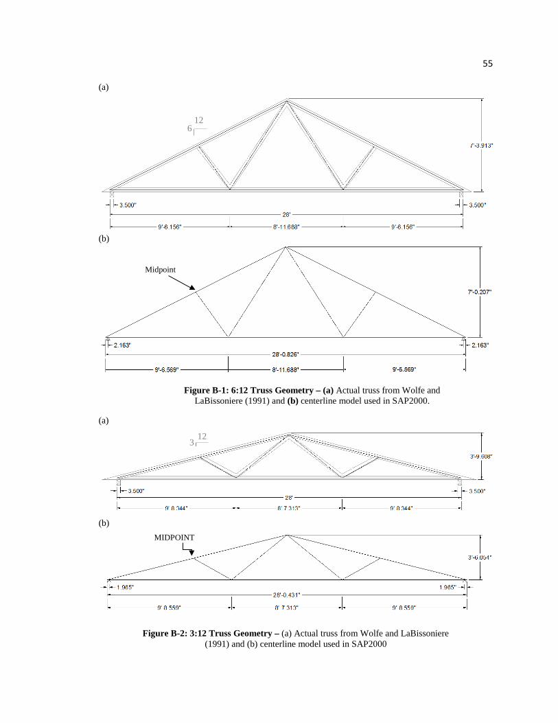
55
(a)
(b)
Figure B-1: 6:12 Truss Geometry – (a) Actual truss from Wolfe and
LaBissoniere (1991) and (b) centerline model used in SAP2000.
(a)
(b)
Figure B-2: 3:12 Truss Geometry – (a) Actual truss from Wolfe and LaBissoniere
(1991) and (b) centerline model used in SAP2000
12 6
Midpoint
12 3
MIDPOINT

56
Each framing member was assigned a cross section equal to the actual cross section of
the lumber used by Wolfe et al. (1986). The connections between members were
idealized as either pinned or rigid based on previous studies conducted by Li (1996) and
Martin (2010). Pinned connections were used at the ridge and the ends of each web,
while rigid connections were used at the truss heels. The splice in the bottom chord of
the truss was modeled both as a pinned connection and as a rigid connection, and proved
to have negligible effect on the stiffness of the truss model. Figure B-3 shows the
connectivity used in the truss models as well as the joint and member labels. Martin
(2010) created a similar pinned and rigid model, which closely followed the geometry
used by Li (1996) (K. Martin, personal communication, July 27, 2010).
Figure B-3: Connectivity and Element Labels for 2D Truss Model –J3 was restrained in the R2 direction (in-plane rotation) to prevent instability warnings.
Three sets of material properties for the framing members were explored in this
study. First, the 6:12 trusses were modeled using the exact MOEs listed by Wolfe et al.
(1986) for each individual member. This allowed for the most accurate comparison
between the tested trusses and the modeled trusses. A list of MOEs is included in Table
B-1. To simplify the model for practical use in the three-dimensional roof assemblies
modeled in Appendix C, the 6:12 and 3:12 trusses were then modeled using average
MOEs for each stiffness category applied uniformly to every member of the truss.
Averaged MOEs for each category and truss slope are listed in Table B-2.
J2 J4 B
J5 J1
A
J3 Pinned Connection Rigid Connection
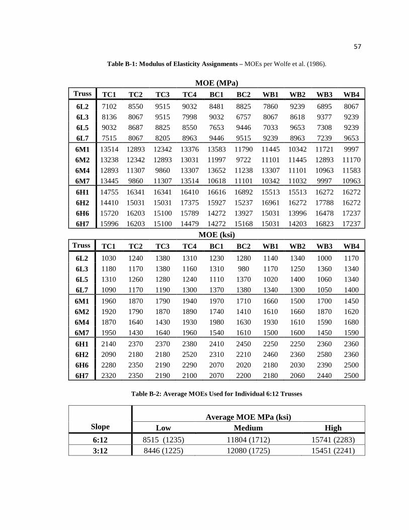
57
Table B-1: Modulus of Elasticity Assignments – MOEs per Wolfe et al. (1986).
MOE (MPa) Truss TC1 TC2 TC3 TC4 BC1 BC2 WB1 WB2 WB3 WB4 6L2 7102 8550 9515 9032 8481 8825 7860 9239 6895 8067 6L3 8136 8067 9515 7998 9032 6757 8067 8618 9377 9239 6L5 9032 8687 8825 8550 7653 9446 7033 9653 7308 9239 6L7 7515 8067 8205 8963 9446 9515 9239 8963 7239 9653 6M1 13514 12893 12342 13376 13583 11790 11445 10342 11721 9997 6M2 13238 12342 12893 13031 11997 9722 11101 11445 12893 11170 6M4 12893 11307 9860 13307 13652 11238 13307 11101 10963 11583 6M7 13445 9860 11307 13514 10618 11101 10342 11032 9997 10963 6H1 14755 16341 16341 16410 16616 16892 15513 15513 16272 16272 6H2 14410 15031 15031 17375 15927 15237 16961 16272 17788 16272 6H6 15720 16203 15100 15789 14272 13927 15031 13996 16478 17237 6H7 15996 16203 15100 14479 14272 15168 15031 14203 16823 17237
MOE (ksi) Truss TC1 TC2 TC3 TC4 BC1 BC2 WB1 WB2 WB3 WB4 6L2 1030 1240 1380 1310 1230 1280 1140 1340 1000 1170 6L3 1180 1170 1380 1160 1310 980 1170 1250 1360 1340 6L5 1310 1260 1280 1240 1110 1370 1020 1400 1060 1340 6L7 1090 1170 1190 1300 1370 1380 1340 1300 1050 1400 6M1 1960 1870 1790 1940 1970 1710 1660 1500 1700 1450 6M2 1920 1790 1870 1890 1740 1410 1610 1660 1870 1620 6M4 1870 1640 1430 1930 1980 1630 1930 1610 1590 1680 6M7 1950 1430 1640 1960 1540 1610 1500 1600 1450 1590 6H1 2140 2370 2370 2380 2410 2450 2250 2250 2360 2360 6H2 2090 2180 2180 2520 2310 2210 2460 2360 2580 2360 6H6 2280 2350 2190 2290 2070 2020 2180 2030 2390 2500 6H7 2320 2350 2190 2100 2070 2200 2180 2060 2440 2500
Table B-2: Average MOEs Used for Individual 6:12 Trusses
Average MOE MPa (ksi)
Slope Low Medium High 6:12 8515 (1235) 11804 (1712) 15741 (2283) 3:12 8446 (1225) 12080 (1725) 15451 (2241)

58
Finally, the trusses were assigned a uniform design MOE determined from the
2005 edition of the NDS National Design Specification for Wood Construction. Based
on Table 4B from AF&PA (2005a), an MOE value of 11030 MPa (1600 ksi) was chosen
for No. 2 grade Southern Pine lumber. No adjustment factors were used since the
members were assumed to be of normal moisture content, with no incisions and tested at
normal temperatures. This MOE value was applied to both the 3:12 and 6:12 trusses and
compared to the overall average deflection of trusses listed in the deflection tables of
Wolfe et al. (1986) regardless of MOE category.
The truss models were loaded with the same truss loads used by Wolfe et al.
(1986): 0.96 kN/m (66 lb/ft) applied along the top chords of the 6:12 trusses and 0.80
kN/m (55 lb/ft) applied along the top chord of the 3:12 truss. The deflections from joints
J1 through J3 were then averaged and compared to the deflections reported by Wolfe et
al. (1986).
Results and Discussion
The resulting deflections for each truss model with exact MOE’s and averaged
MOE’s are included in Tables B-3 through B-5. For both the exact MOEs and the
averaged MOEs, the models were able to predict the average deflection of the trusses in
each stiffness category within 10% of the actual deflections listed by Wolfe et al. 1986.
Martin (2010) managed to reduce this discrepancy to less than 5 percent, mainly due to
differences in the geometry used to simulate the trusses. As stated before, Martin (2010)
used a truss model that was similar to the geometry used by Li (1996), which was 20.3
mm (0.8 in) taller and 88.2 mm (3.47 in) wider than the current model, with the same
clear-span.
The models that were assigned a design MOE from AF&PA (2005a) predicted the
overall average deflection for both the 3:12 sloped trusses and the 6:12 sloped trusses
within 5% of the deflections reported by Wolfe et al. (1986). Table B-6 shows results for
the trusses modeled with AF&PA (2005a) properties. In all cases, the truss models were
stiffer than the actual tested trusses. This is likely due to the use of a rigid connection at
the heels of the truss as opposed to a more realistic semi-rigid connection.

59
Table B-3: Comparison of Experimental and Model Displacements – Percent differences between computer models and the experimental data of Wolfe et al. (1986).
Wolfe et al. (1986) Current Study Martin (2010)
Truss Deflection Deflection % Diff. from Deflection % Diff.
from
mm (in) mm (in) Wolfe et al. (1986) mm (in) Wolfe et
al. (1986) 6L2 4.369 (0.172) 4.318 (0.170) -1% 4.547 (0.179) 4% 6L3 4.572 (0.180) 4.496 (0.177) -2% 4.724 (0.186) 3% 6L5 4.927 (0.194) 4.267 (0.168) -14% 4.470 (0.176) -9% 6L7 5.029 (0.198) 4.242 (0.167) -16% 4.445 (0.175) -12%
Average 4.724 (0.186) 4.318 (0.170) -8% 4.547 (0.179) -4% 6M1 3.124 (0.123) 2.870 (0.113) -8% 2.997 (0.118) -4% 6M2 3.454 (0.136) 3.099 (0.122) -11% 3.226 (0.127) -7% 6M4 3.073 (0.121) 3.048 (0.120) -1% 3.200 (0.126) 4% 6M7 2.972 (0.117) 3.200 (0.126) 8% 3.353 (0.132) 13%
Average 3.150 (0.124) 3.048 (0.120) -3% 3.200 (0.126) 1% 6H1 2.718 (0.107) 2.260 (0.089) -17% 2.388 (0.094) -12% 6H2 2.718 (0.107) 2.362 (0.093) -13% 2.464 (0.097) -9% 6H6 2.184 (0.086) 2.438 (0.096) 12% 2.565 (0.101) 17% 6H7 2.718 (0.107) 2.413 (0.095) -11% 2.591 (0.102) -5%
Average 2.591 (0.102) 2.362 (0.093) -8% 2.515 (0.099) -3%
Table B-4: Comparison of Average Displacements for Simplified 6:12 Trusses using Average MOE Values
Wolfe et al. (1986) Current Study with Averaged MOEs
Truss Average Disp. Average Disp. % Diff. from
mm (in) mm (in) Wolfe et al. (1986) Average L 4.724 (0.186) 4.293 (0.169) -9% Average M 3.150 (0.124) 3.100 (0.122) -2% Average H 2.591 (0.102) 2.311 (0.091) -10%

60
Table B-5: Comparison of Average Displacements for 3:12 Trusses using Average MOE Values - *Note that the deflection tables found in Wolfe et al. (1986) are inconsistent. The average deflections in the 6:12 tables were calculated using the deflection = A x (design load ratio) + B equation found at the top of the table, whereas the average deflections for the 3:12 tables were calculated from Column A only. This inconsistency has been corrected in Table A-9 so that the 3:12 averages also incorporate the straight line deflection equation.
Wolfe et al. (1986) Current Study with Averaged MOEs
Truss Average Disp. Average Disp. % Diff. from
mm (in) mm (in) Wolfe et al. (1986) Average L 11.66 (0.459) 11.30 (0.445) -3% Average M 8.204 (0.323) 8.026 (0.316) -2% Average H 6.833 (0.269) 6.172 (0.243) -9%
Table B-6: Comparison of Average Displacements for trusses with AF&PA (2005a)
design MOE
Wolfe et al. (1986) Current Study with AF&PA (2005a) Design MOE
Truss Total Average Disp. Average Disp. % Diff. from
mm (in) mm (in) Wolfe et al. (1986) 3:12 Slope 8.890 (0.350) 8.636 (0.340) -3% 6:12 Slope 3.480 (0.137) 3.327 (0.131) -5%
Conclusions
The simplified, linear modeling techniques described in this appendix are
sufficient for predicting the behavior of two-dimensional trusses with various pitches and
stiffness. Based on the results described above, the following methods were adopted for
use in the current study:
• Pinned connections were used at the ends of each web member and at the ridge
of the truss. Rigid connections were used along top chords, bottom chords and at
truss heels. Figure B-3 shows the connectivity used in the truss models.
• Truss chords and web members were modeled using the SAP2000 frame element
with an assigned cross section equal to the actual cross section of the member.

61
• Material properties for the framing members were assumed to be linear and
isotropic. The modulus of elasticity for each member was determined using
design properties listed in AF&PA (2005a).
For the three-dimensional truss assembly validation described in Appendix C, the average
MOE from Wolfe et al. (1986) for each stiffness category was used in lieu of AF&PA
(2005a) design properties so the effects of varying truss stiffness within the assembly
could be explored.

62
APPENDIX C
THREE DIMENSIONAL ROOF ASSEMBLY MODEL VALIDATION
Introduction
Methods for modeling roof assemblies were validated against full- scale tests
performed by Wolfe and McCarthy (1989) on two nine-truss gable roof assemblies. One
assembly had a 3:12 roof pitch and the other had a 6:12 roof pitch. The trusses,
constructed by Wolfe et al. (1986), were spaced 0.61 m (2 ft) on center. As in Wolfe et
al. (1986), the trusses were grouped into high (H), medium (M), and low (L) Modulus of
Elasticity (MOE) categories based on the individual MOE’s of the 2x4 members used to
construct the trusses. Within the assemblies, trusses were arranged into a pattern of: M-
H-L-M-H-L-L-M-H moving from West to East based on MOE category as shown in
Figure C-1.
Figure C-1: Pattern of Truss Stiffness in Assemblies – Low MOE (L), Medium MOE
(M) and High MOE (H) as used by Wolfe and McCarthy (1989)
West
East
North
South
L
H
M
L
H
M
L
H
M

63
The sheathing used in the assembly was 11.9-mm-thick (15/32-in-thick) Southern
Pine 3-ply plywood. The average bending stiffness (EI) of the plywood was measured by
Wolfe and McCarthy (1989) using a plate bending test and found to be 1.19 N·m2/m
(196,000 lb·in2/ft). The assembly was supported along the north and south sides by 0.9-
m-tall (3-ft-tall) wood framed walls with a clear span of 8.4 m (27 ft, 5 in).
Modeling Methods
Individual Trusses
The trusses in the current study were modeled as described in Appendix B, using
only pinned and rigid connections. The MOE for each of the stiffness categories was
determined by averaging the individual MOE’s of the 2x4’s used to construct each of the
trusses as shown in Tables C-1 and C-2. The self-weight of the material was not included
in the model.
Table C-1: Average MOE’s used for Trusses* in 3:12 Truss Assembly
Average MOE MPa (ksi) Low: *3L2, 3L4, 3L6 Medium: *3M2, 3M4, 3M6 High: *3H1, 3H3, 3H5
8667 (1257) 11004 (1596) 16443 (2383)
Table C-2: Average MOE’s used for Trusses* in 6:12 Truss Assembly
Average MOE MPa (ksi) Low: *6L1, 6L4, 6L6 Medium: *6M3, 6M5, 6M6 High: *6H3, 6H4, 6H5
8450 (1226) 12080 (1752) 16171 (2345)
Plywood Sheathing
The sheathing was represented using a continuous, orthotropic “Layered Shell
Element” from SAP2000, with a thickness of 11.9 mm (0.469 in) and local coordinates
oriented as shown in Figure C-2. The sheathing layer was displaced 50.4 mm (1.98 in)
from the centerline of the top chord framing members towards the top surface of the
assembly. This was done so that the plywood is modeled at its true physical location
rather than through the centerlines of the top chords.

64
Figure C-2: Local Coordinate Orientation of Thick Shell Elements for Sheathing –
with strong axis (1) running perpendicular to the truss supports
Material properties for the plywood sheathing were calculated using
experimentally determined values provided by Wolfe and McCarthy (1989), as well as
design specifications and publically available software. A moment of inertia (I) of
1.41x10⁻⁷ m4/m (0.103 in4/ft) was determined using the 2008 APA Panel Design
Specification for 32/15-in-thick, 3-ply plywood from Species Group 1. The MOE along
the strong axis (“E1” as designated by SAP2000) was then determined by dividing the
measured EI from Wolfe and McCarthy (1989) by the moment of inertia suggested by
APA (2008) to give an MOE of 13,120 MPa (1,903 ksi).
Martin (2010), found the most sensitive material properties for the sheathing to be
the MOE along the strong and weak axes (E1 and E2 in SAP2000), the in-plane shear
modulus (G12 in SAP2000), and the Poisson’s Ratio related to E2 (u12). It is important to
note that the subscript notation for Poisson’s Ratio in SAP2000 is the inverse of
conventional notation, where νij is typically related to Ei as illustrated in Figure C-3.
1
2
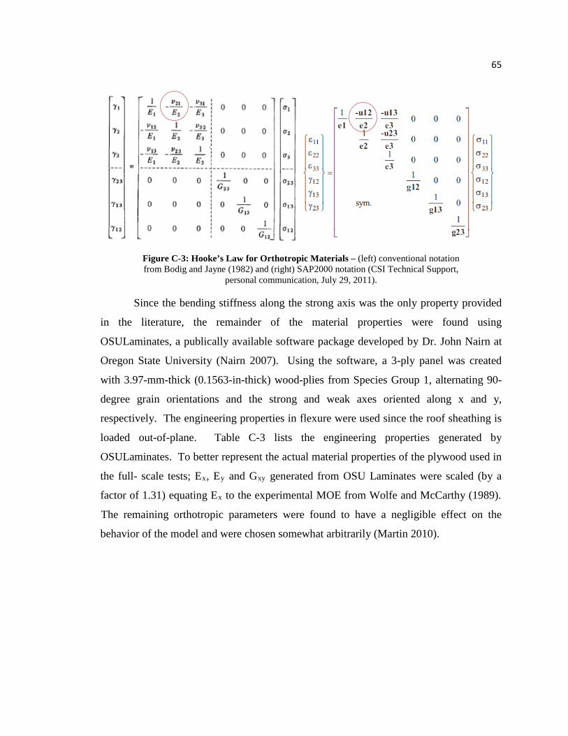
65
Figure C-3: Hooke’s Law for Orthotropic Materials – (left) conventional notation from Bodig and Jayne (1982) and (right) SAP2000 notation (CSI Technical Support,
personal communication, July 29, 2011).
Since the bending stiffness along the strong axis was the only property provided
in the literature, the remainder of the material properties were found using
OSULaminates, a publically available software package developed by Dr. John Nairn at
Oregon State University (Nairn 2007). Using the software, a 3-ply panel was created
with 3.97-mm-thick (0.1563-in-thick) wood-plies from Species Group 1, alternating 90-
degree grain orientations and the strong and weak axes oriented along x and y,
respectively. The engineering properties in flexure were used since the roof sheathing is
loaded out-of-plane. Table C-3 lists the engineering properties generated by
OSULaminates. To better represent the actual material properties of the plywood used in
the full- scale tests; Ex, Ey and Gxy generated from OSU Laminates were scaled (by a
factor of 1.31) equating Ex to the experimental MOE from Wolfe and McCarthy (1989).
The remaining orthotropic parameters were found to have a negligible effect on the
behavior of the model and were chosen somewhat arbitrarily (Martin 2010).

66
Table C-3: Engineering Properties in Bending for 3-Ply Panel Generated by OSU Laminates and scaled to Wolfe and McCarthy (1989) – Scaled properties are used in
the model
Orthotropic Properties Generated from OSU Laminates
Scaled to Wolfe and McCarthy (1989)
Ex (E1 in SAP2000)
MPa
(ksi
) 9991 (1449) 13120 (1903)
Ey (E2 in SAP2000) 669 (97) 878 (127)
Gxy (G12 in SAP2000) 483 (70) 634 (92)
vyx (u12 in SAP2000) 0.011 0.011
Meshing and Boundary Conditions
As in Martin (2010), the roof sheathing was meshed into elements with a
maximum size of 610 mm (24 in) so that the sheathing elements would align with the
framing elements of the trusses. This was accomplished using the Automatic Mesh tool
in SAP2000.
With respect to boundary conditions, it was reported that the “supports within the
assembly behaved as something between [pinned] and roller” (Wolfe and McCarthy
1989). The current study used the “roller-roller” conditions shown in Figure C-4, with
horizontal restraint provided at the line of symmetry at the peak. Lateral displacements
were measured in the U1 direction at the roller supports of the model during loading and
were found to be less than 0.87 mm (0.034 in), which is consistent with the maximum
displacement of 0.89 mm (0.035 in) reported by Wolfe and McCarthy (1989).

67
Figure C-4: “Roller-Roller” Support Conditions – for each truss the heel supports are restrained in the U3 (vertical) direction only. The ridge at each end of the assembly is
also restrained in the U1 and U2 (lateral) directions to prevent instability warnings.
Loading and Data Collection
Following procedures outlined in Wolfe and McCarthy (1989), the trusses in both
the 3:12- and 6:12-sloped assemblies were loaded one at a time. The trusses in the 3:12
assembly were loaded with 803 N/m (55 lb/ft) uniformly distributed along the top chord,
and the trusses in the 6:12 assembly were loaded with 963 N/m (66 lb/ft). For each
loaded truss, the relative vertical deflections and support reactions of every truss in the
assembly were measured and plotted against the results reported in the literature.
Relative vertical reactions (Rrel) were determined as the ratio of the total vertical
support reaction at each individual truss to the total load applied to the assembly as
shown in Equation C-1. For the 3:12 assembly, the total load for a distributed load of
803 N/m (55 lb/ft) along the top chord of a truss was found to be 7068 N (1589 lb). For
the 6:12 assembly, the total load for a distributed load of 963 N/m (66 lb/ft) along the top
chord of a truss was found to be 9212 N (2071 lb).
𝑅𝑅𝑟𝑟𝑟𝑟𝑟𝑟,𝑗𝑗 = 𝑅𝑅𝑗𝑗∑ 𝑅𝑅𝑖𝑖9𝑖𝑖=1
𝑥𝑥 100% 𝐹𝐹𝐹𝐹𝐹𝐹 𝑗𝑗 = 1 𝑡𝑡𝐹𝐹 9 Equation C-1
Note that in Equation C-1, i and j refer to individual trusses within the assembly,
where truss 1 is located on the West side of the assembly, and truss 9 is located on the

68
East side of the assembly. This notation was used for all tables and charts related to the
roof assembly validation.
Deflections were measured at four locations on each truss, as shown in Figure C-
5, and averaged to determine the average deflection (Δavg) at each truss. The average
deflections of all trusses were then summed to give the total average deflection of the
assembly. In accordance with Wolfe and McCarthy (1989), the percent contribution of
an individual truss to the total average deflection of the assembly was defined as the
“relative deflection” of that truss. The relative deflections (Δrel) were calculated as shown
in Equation C-2.
Figure C-5: Locations for Deflection Measurement on Each Truss – The average
deflection (Δavg) at each truss was calculated as the average of the deflections measured at each of the four locations shown.
𝛥𝛥𝑟𝑟𝑟𝑟𝑟𝑟,𝑗𝑗 = ∆𝑎𝑎𝑎𝑎𝑎𝑎,𝑗𝑗
∑ ∆𝑎𝑎𝑎𝑎𝑎𝑎,𝑖𝑖9𝑖𝑖=1
𝑥𝑥 100% 𝐹𝐹𝐹𝐹𝐹𝐹 𝑗𝑗 = 1 𝑡𝑡𝐹𝐹 9 Equation C-2
Results and Discussion
Relative deflections and reactions for the 3:12 and 6:12 assembly models were
plotted against results from Wolfe and McCarthy (1989) and organized into influence
matrices as shown in Appendix D. The percent error in relative deflections and reactions
at the loaded trusses were calculated based on the full- scale tests. At the loaded trusses,
relative reactions were predicted with an average error of 9 percent from the full-scale
tests in the 3:12 assembly and 17 percent in the 6:12 assembly as shown in Table C-4.
Relatively high errors were seen at trusses 2, 5, 6 and 8 in the 6:12 assembly, however,
there is not enough information to determine why errors were high at these trusses. Both
models accurately predicted the overall load distributions to non-loaded trusses as shown
in Figures D-1 through D-18 in Appendix D.
North South

69
Table C-4: Absolute Error in Predicted Relative Reactions at Loaded Trusses in Each Assembly – Compared to Wolfe and McCarthy (1989)
Loaded Truss #
Percent Error
3:12 Assembly 6:12 Assembly
1 3% 7% 2 18% 32% 3 20% 11% 4 1% 11% 5 7% 26% 6 13% 25% 7 11% 7% 8 3% 27% 9 9% 7%
Average 9% 17%
Although the main focus of this study is force distribution through the structure,
the relative deflections were also checked to provide additional validation as shown in
Table C-5.
Table C-5: Absolute Error in Predicted Relative Deflections at Loaded Trusses in Each Assembly – Compared to Wolfe and McCarthy (1989)
Loaded Truss #
Percent Error 3:12 Assembly 6:12 Assembly
1 10% 9% 2 24% 15% 3 38% 0% 4 45% 14% 5 16% 8% 6 30% 9% 7 21% 4% 8 10% 11% 9 21% 0%
Average 24% 8%
At the loaded trusses, the 3:12 model predicted relative deflections with an
average error of 24 percent compared to Wolfe and McCarthy (1989). The 6:12
assembly more accurately predicted relative deflections with an average error of only 8
percent. It was observed that the 3:12 model was more accurate in predicting force

70
distributions than deflections while the 6:12 assembly was more accurate in predicting
deflections than force distributions. The reason for this discrepancy is unknown. Overall
distributions of relative deflections for each loading scenario were plotted in Figures D-
19 through D-36.
Conclusions
The two nine-truss gable roof assemblies with varying slope and individual truss
stiffness were adequate in predicting assembly behavior. Based on the results in this
appendix, the following modeling methods were adopted for use in the current study:
• Roof sheathing was modeled using a continuous “layered shell element” from
SAP2000.
• The plywood layer was displaced from the centerline of the truss top chord so that
the bottom surface of the plywood was even with the top surface of the truss top-
chord cross section.
• Material properties for the plywood sheathing were assumed to be orthotropic and
were determined using flexural engineering properties calculated by OSU
Laminates Software.

71
APPENDIX D
PLOTS FOR ROOF ASSEMBLY MODEL VALIDATION
This appendix contains influence matrices and plots for the 3:12 and 6:12
assemblies that were modeled in Appendix C.
3:12 Assembly – Relative Reactions
Figure D-1: Relative Reactions for 3:12 Truss Assembly When Truss 1 is Loaded
-15%
-5%
5%
15%
25%
35%
45%
55%
65%
75%
1 2 3 4 5 6 7 8 9
Perc
ent o
f Tot
al R
eact
ion
Truss #
Relative Reactions (Truss 1 Loaded) - 3/12 Assembly
Wolfe and McCarthy 1989
Current Study

72
Figure D-2: Relative Reactions for 3:12 Truss Assembly When Truss 2 is Loaded
Figure D-3: Relative Reactions for 3:12 Truss Assembly When Truss 3 is Loaded
-15%
-5%
5%
15%
25%
35%
45%
55%
65%
75%
1 2 3 4 5 6 7 8 9
Perc
ent o
f Tot
al R
eact
ion
Truss #
Relative Reactions (Truss 2 Loaded) - 3/12 Assembly
Wolfe and McCarthy (1989)
Current Study
-15%
-5%
5%
15%
25%
35%
45%
55%
65%
75%
1 2 3 4 5 6 7 8 9
Perc
ent o
f Tot
al R
eact
ion
Truss #
Relative Reactions (Truss 3 Loaded) - 3/12 Assembly
Wolfe and McCarthy (1989)Current Study
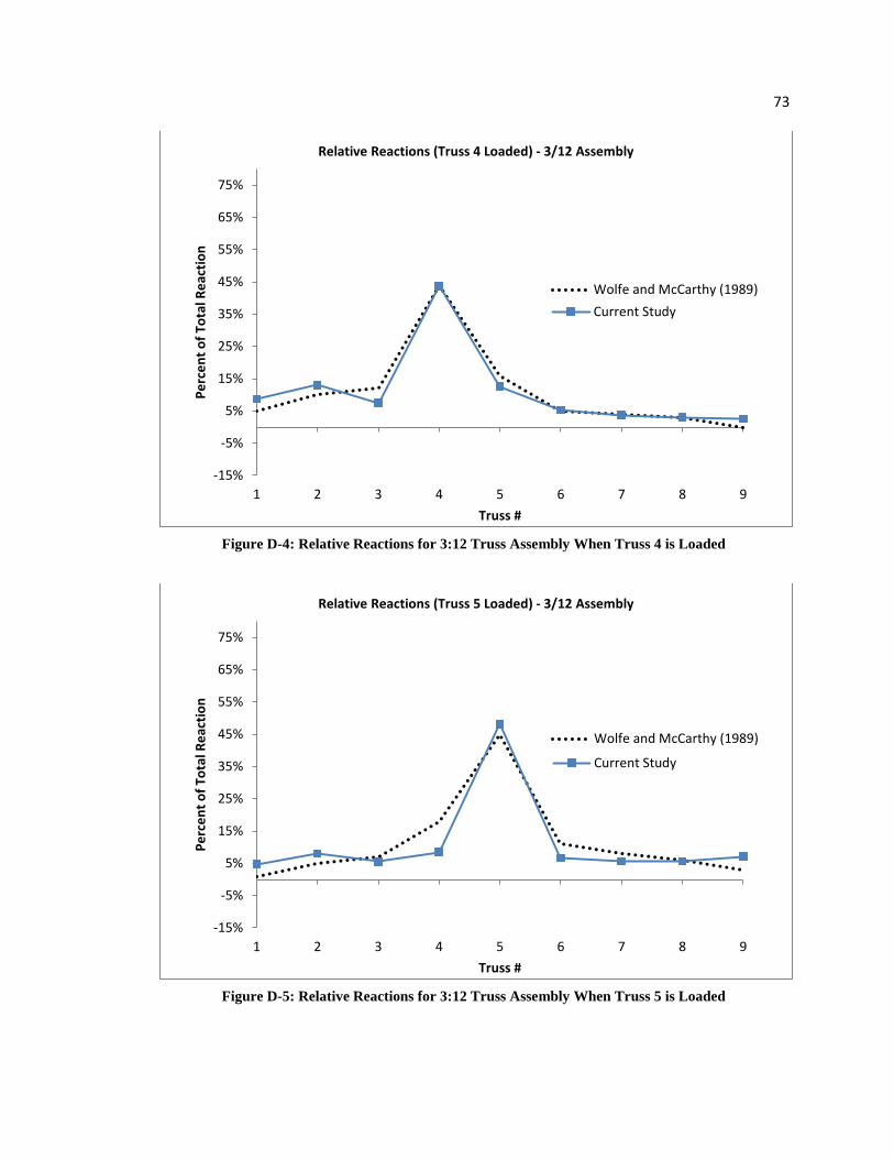
73
Figure D-4: Relative Reactions for 3:12 Truss Assembly When Truss 4 is Loaded
Figure D-5: Relative Reactions for 3:12 Truss Assembly When Truss 5 is Loaded
-15%
-5%
5%
15%
25%
35%
45%
55%
65%
75%
1 2 3 4 5 6 7 8 9
Perc
ent o
f Tot
al R
eact
ion
Truss #
Relative Reactions (Truss 4 Loaded) - 3/12 Assembly
Wolfe and McCarthy (1989)Current Study
-15%
-5%
5%
15%
25%
35%
45%
55%
65%
75%
1 2 3 4 5 6 7 8 9
Perc
ent o
f Tot
al R
eact
ion
Truss #
Relative Reactions (Truss 5 Loaded) - 3/12 Assembly
Wolfe and McCarthy (1989)
Current Study

74
Figure D-6: Relative Reactions for 3:12 Truss Assembly When Truss 6 is Loaded
Figure D-7: Relative Reactions for 3:12 Truss Assembly When Truss 7 is Loaded
-15%
-5%
5%
15%
25%
35%
45%
55%
65%
75%
1 2 3 4 5 6 7 8 9
Perc
ent o
f Tot
al R
eact
ion
Truss #
Relative Reactions (Truss 6 Loaded) - 3/12 Assembly
Wolfe and McCarthy (1989)
Current Study
-15%
-5%
5%
15%
25%
35%
45%
55%
65%
75%
1 2 3 4 5 6 7 8 9
Perc
ent o
f Tot
al R
eact
ion
Truss #
Relative Reactions (Truss 7 Loaded) - 3/12 Assembly
Wolfe and McCarthy (1989)
Current Study

75
Figure D-8: Relative Reactions for 3:12 Truss Assembly When Truss 8 is Loaded
Figure D-9: Relative Reactions for 3:12 Truss Assembly When Truss 9 is Loaded
-15%
-5%
5%
15%
25%
35%
45%
55%
65%
75%
1 2 3 4 5 6 7 8 9
Perc
ent o
f Tot
al R
eact
ion
Truss #
Relative Reactions (Truss 8 Loaded) - 3/12 Assembly
Wolfe and McCarthy (1989)
Current Study
-15%
-5%
5%
15%
25%
35%
45%
55%
65%
75%
1 2 3 4 5 6 7 8 9
Perc
ent o
f Tot
al R
eact
ion
Truss #
Relative Reactions (Truss 9 Loaded) - 3/12 Assembly
Wolfe and McCarthy (1989)
Current Study

76
Influence Matrices for 3:12 Assembly – Relative Reactions
Table D-1: Relative Reactions of Trusses in 3:12 Assembly from Wolfe and McCarthy (1989)
Loaded Truss Relative Reactions at Truss # 1 2 3 4 5 6 7 8 9
1 57% 29% 12% 10% 3% 0% -1% -4% -8% 2 20% 49% 18% 11% 6% 2% 0% -1% -2% 3 10% 20% 36% 20% 7% 3% 2% 1% -1% 4 5% 10% 12% 44% 16% 5% 4% 3% 0% 5 1% 5% 7% 18% 45% 11% 8% 6% 3% 6 0% 3% 5% 8% 17% 37% 13% 9% 7% 7 -1% 1% 3% 5% 9% 12% 39% 19% 13% 8 -2% -2% 1% 3% 6% 6% 16% 48% 24% 9 -4% -4% -1% 0% 4% 6% 10% 26% 63%
Table D-2: Relative Reactions of Trusses in 3:12 Assembly from Current Study
Loaded Truss Relative Reactions at Truss # 1 2 3 4 5 6 7 8 9
1 58% 28% 11% 9% 7% 1% -1% -4% -10% 2 19% 58% 10% 9% 8% 2% 1% -1% -5% 3 13% 19% 43% 9% 10% 4% 2% 1% -1% 4 9% 13% 7% 44% 13% 5% 4% 3% 3% 5 5% 8% 6% 8% 48% 7% 6% 6% 7% 6 2% 4% 4% 7% 13% 42% 8% 9% 12% 7 -1% 1% 2% 5% 11% 8% 43% 12% 19% 8 -4% -2% 1% 3% 8% 7% 10% 50% 27% 9 -7% -5% -1% 2% 7% 7% 10% 18% 69%
Table D-3: Difference in Relative Reactions for 3:12 Assembly
Loaded Truss Difference in Relative Reactions: (Wolfe and McCarthy 1989) - (Current Study) 1 2 3 4 5 6 7 8 9
1 -1% 1% 1% 1% -4% -1% 0% 0% 2% 2 1% -9% 8% 2% -2% 0% -1% 0% 3% 3 -3% 1% -7% 11% -3% -1% 0% 0% 0% 4 -4% -3% 5% 0% 3% 0% 0% 0% -3% 5 -4% -3% 1% 10% -3% 4% 2% 0% -4% 6 -2% -1% 1% 1% 4% -5% 5% 0% -5% 7 0% 0% 1% 0% -2% 4% -4% 7% -6% 8 2% 0% 0% 0% -2% -1% 6% -2% -3% 9 3% 1% 0% -2% -3% -1% 0% 8% -6%

77
6:12 Assembly – Relative Reactions
Figure D-10: Relative Reactions for 6:12 Truss Assembly When Truss 1 is Loaded
Figure D-11: Relative Reactions for 6:12 Truss Assembly When Truss 2 is Loaded
-15%
-5%
5%
15%
25%
35%
45%
55%
65%
75%
1 2 3 4 5 6 7 8 9
Perc
ent o
f Tot
al R
eact
ion
Truss #
Relative Reactions (Truss 1 Loaded) - 6/12 Assembly
Wolfe and McCarthy (1989)Current Study
-15%
-5%
5%
15%
25%
35%
45%
55%
65%
75%
1 2 3 4 5 6 7 8 9
Perc
ent o
f Tot
al R
eact
ion
Truss #
Relative Reactions (Truss 2 Loaded) - 6/12 Assembly
Wolfe and McCarthy (1989)
Current Study

78
Figure D-12: Relative Reactions for 6:12 Truss Assembly When Truss 3 is Loaded
Figure D-13: Relative Reactions for 6:12 Truss Assembly When Truss 4 is Loaded
-15%
-5%
5%
15%
25%
35%
45%
55%
65%
75%
1 2 3 4 5 6 7 8 9
Perc
ent o
f Tot
al R
eact
ion
Truss #
Relative Reactions (Truss 3 Loaded) - 6/12 Assembly
Wolfe and McCarthy (1989)
Current Study
-15%
-5%
5%
15%
25%
35%
45%
55%
65%
75%
1 2 3 4 5 6 7 8 9
Perc
ent o
f Tot
al R
eact
ion
Truss #
Relative Reactions (Truss 4 Loaded) - 6/12 Assembly
Wolfe and McCarthy (1989)Current Study

79
Figure D-14: Relative Reactions for 6:12 Truss Assembly When Truss 5 is Loaded
Figure D-15: Relative Reactions for 6:12 Truss Assembly When Truss 6 is Loaded
-15%
-5%
5%
15%
25%
35%
45%
55%
65%
75%
1 2 3 4 5 6 7 8 9
Perc
ent o
f Tot
al R
eact
ion
Truss #
Relative Reactions (Truss 5 Loaded) - 6/12 Assembly
Wolfe and McCarthy (1989)Current Study
-15%
-5%
5%
15%
25%
35%
45%
55%
65%
75%
1 2 3 4 5 6 7 8 9
Perc
ent o
f Tot
al R
eact
ion
Truss #
Relative Reactions (Truss 6 Loaded) - 6/12 Assembly
Wolfe and McCarthy (1989)
Current Study

80
Figure D-16: Relative Reactions for 6:12 Truss Assembly When Truss 7 is Loaded
Figure D-17: Relative Reactions for 6:12 Truss Assembly When Truss 8 is Loaded
-15%
-5%
5%
15%
25%
35%
45%
55%
65%
75%
1 2 3 4 5 6 7 8 9
Perc
ent o
f Tot
al R
eact
ion
Truss #
Relative Reactions (Truss 7 Loaded) - 6/12 Assembly
Wolfe and McCarthy (1989)Current Study
-15%
-5%
5%
15%
25%
35%
45%
55%
65%
75%
1 2 3 4 5 6 7 8 9
Perc
ent o
f Tot
al R
eact
ion
Truss #
Relative Reactions (Truss 8 Loaded) - 6/12 Assembly
Wolfe and McCarthy (1989)Current Study
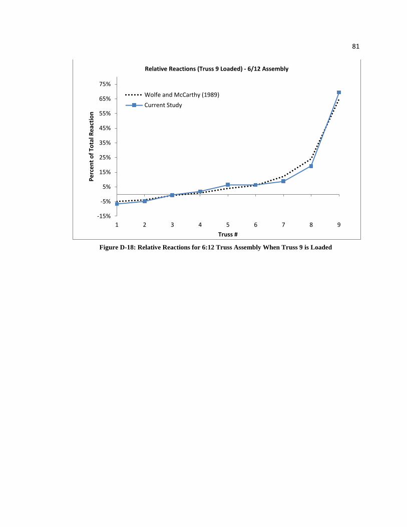
81
Figure D-18: Relative Reactions for 6:12 Truss Assembly When Truss 9 is Loaded
-15%
-5%
5%
15%
25%
35%
45%
55%
65%
75%
1 2 3 4 5 6 7 8 9
Perc
ent o
f Tot
al R
eact
ion
Truss #
Relative Reactions (Truss 9 Loaded) - 6/12 Assembly
Wolfe and McCarthy (1989)Current Study
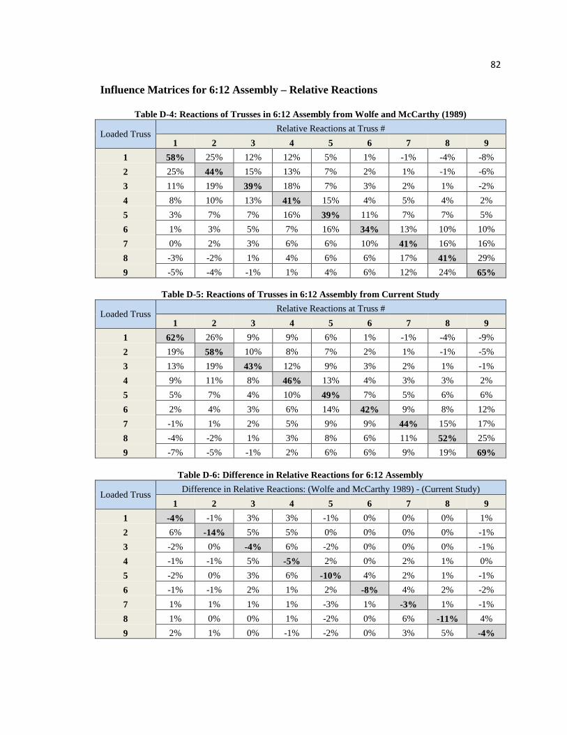
82
Influence Matrices for 6:12 Assembly – Relative Reactions
Table D-4: Reactions of Trusses in 6:12 Assembly from Wolfe and McCarthy (1989)
Loaded Truss Relative Reactions at Truss # 1 2 3 4 5 6 7 8 9
1 58% 25% 12% 12% 5% 1% -1% -4% -8% 2 25% 44% 15% 13% 7% 2% 1% -1% -6% 3 11% 19% 39% 18% 7% 3% 2% 1% -2% 4 8% 10% 13% 41% 15% 4% 5% 4% 2% 5 3% 7% 7% 16% 39% 11% 7% 7% 5% 6 1% 3% 5% 7% 16% 34% 13% 10% 10% 7 0% 2% 3% 6% 6% 10% 41% 16% 16% 8 -3% -2% 1% 4% 6% 6% 17% 41% 29% 9 -5% -4% -1% 1% 4% 6% 12% 24% 65%
Table D-5: Reactions of Trusses in 6:12 Assembly from Current Study
Loaded Truss Relative Reactions at Truss # 1 2 3 4 5 6 7 8 9
1 62% 26% 9% 9% 6% 1% -1% -4% -9% 2 19% 58% 10% 8% 7% 2% 1% -1% -5% 3 13% 19% 43% 12% 9% 3% 2% 1% -1% 4 9% 11% 8% 46% 13% 4% 3% 3% 2% 5 5% 7% 4% 10% 49% 7% 5% 6% 6% 6 2% 4% 3% 6% 14% 42% 9% 8% 12% 7 -1% 1% 2% 5% 9% 9% 44% 15% 17% 8 -4% -2% 1% 3% 8% 6% 11% 52% 25% 9 -7% -5% -1% 2% 6% 6% 9% 19% 69%
Table D-6: Difference in Relative Reactions for 6:12 Assembly
Loaded Truss Difference in Relative Reactions: (Wolfe and McCarthy 1989) - (Current Study) 1 2 3 4 5 6 7 8 9
1 -4% -1% 3% 3% -1% 0% 0% 0% 1% 2 6% -14% 5% 5% 0% 0% 0% 0% -1% 3 -2% 0% -4% 6% -2% 0% 0% 0% -1% 4 -1% -1% 5% -5% 2% 0% 2% 1% 0% 5 -2% 0% 3% 6% -10% 4% 2% 1% -1% 6 -1% -1% 2% 1% 2% -8% 4% 2% -2% 7 1% 1% 1% 1% -3% 1% -3% 1% -1% 8 1% 0% 0% 1% -2% 0% 6% -11% 4% 9 2% 1% 0% -1% -2% 0% 3% 5% -4%

83
3:12 Assembly – Relative Deflections
Figure D-19: Relative Deflections for 3:12 Truss Assembly When Truss 1 is Loaded
-15%
-5%
5%
15%
25%
35%
45%
55%
65%
75%
1 2 3 4 5 6 7 8 9
% o
f Tot
al A
vera
ge D
efle
ctio
n
Truss #
Relative Deflections (Truss 1 Loaded) - 3/12 Assembly
Wolfe and McCarthy (1989)
Current Study

84
Figure D-20: Relative Deflections for 3:12 Truss Assembly When Truss 2 is Loaded
Figure D-21: Relative Deflections for 3:12 Truss Assembly When Truss 3 is Loaded
-15%
-5%
5%
15%
25%
35%
45%
55%
65%
75%
1 2 3 4 5 6 7 8 9
% o
f Tot
al A
vera
ge D
efle
ctio
n
Truss #
Relative Deflections (Truss 2 Loaded) - 3/12 Assembly
Wolfe and McCarthy (1989)Current Study
-15%
-5%
5%
15%
25%
35%
45%
55%
65%
75%
1 2 3 4 5 6 7 8 9
% o
f Tot
al A
vera
ge D
efle
ctio
n
Truss #
Relative Deflections (Truss 3 Loaded) - 3/12 Assembly
Wolfe and McCarthy (1989)
Current Study

85
Figure D-22: Relative Deflections for 3:12 Truss Assembly When Truss 4 is Loaded
Figure D-23: Relative Deflections for 3:12 Truss Assembly When Truss 5 is Loaded
-15%
-5%
5%
15%
25%
35%
45%
55%
65%
75%
1 2 3 4 5 6 7 8 9
% o
f Tot
al A
vera
ge D
efle
ctio
n
Truss #
Relative Deflections (Truss 4 Loaded) - 3/12 Assembly
Wolfe and McCarthy (1989)
Current Study
-15%
-5%
5%
15%
25%
35%
45%
55%
65%
75%
1 2 3 4 5 6 7 8 9
% o
f Tot
al A
vera
ge D
efle
ctio
n
Truss #
Relative Deflections (Truss 5 Loaded) - 3/12 Assembly
Wolfe and McCarthy (1989)Current Study

86
Figure D-24: Relative Deflections for 3:12 Truss Assembly When Truss 6 is Loaded
Figure D-25: Relative Deflections for 3:12 Truss Assembly When Truss 7 is Loaded
-15%
-5%
5%
15%
25%
35%
45%
55%
65%
75%
1 2 3 4 5 6 7 8 9
% o
f Tot
al A
vera
ge D
efle
ctio
n
Truss #
Relative Deflections (Truss 6 Loaded) - 3/12 Assembly
Wolfe and McCarthy (1989)
Current Study
-15%
-5%
5%
15%
25%
35%
45%
55%
65%
75%
1 2 3 4 5 6 7 8 9
% o
f Tot
al A
vera
ge D
efle
ctio
n
Truss #
Relative Deflections (Truss 7 Loaded) - 3/12 Assembly
Wolfe and McCarthy (1989)
Current Study

87
Figure D-26: Relative Deflections for 3:12 Truss Assembly When Truss 8 is Loaded
Figure D-27: Relative Deflections for 3:12 Truss Assembly When Truss 9 is Loaded
-15%
-5%
5%
15%
25%
35%
45%
55%
65%
75%
1 2 3 4 5 6 7 8 9
% o
f Tot
al A
vera
ge D
efle
ctio
n
Truss #
Relative Deflections (Truss 8 Loaded) - 3/12 Assembly
Wolfe and McCarthy (1989)Current Study
-15%
-5%
5%
15%
25%
35%
45%
55%
65%
75%
1 2 3 4 5 6 7 8 9
% o
f Tot
al A
vera
ge D
efle
ctio
n
Truss #
Relative Deflections (Truss 9 Loaded) - 3/12 Assembly
Wolfe and McCarthy (1989)Current Study

88
Influence Matrices for 3:12 Assembly – Relative Deflections
Table D-7: Relative Deflections of Trusses in 3:12 Assembly from Wolfe and McCarthy (1989)
Loaded Truss Relative Deflections at Truss #
1 2 3 4 5 6 7 8 9 1 64.9% 26.2% 11.2% 3.4% -0.9% 0.4% -0.8% -0.3% -4.1% 2 27.6% 49.0% 19.3% 5.8% -0.1% 0.8% -0.9% 0.0% -1.5% 3 3.1% 21.3% 56.2% 18.1% 2.2% 2.2% 0.2% -1.2% -2.1% 4 -1.2% 4.0% 25.7% 58.8% 7.9% 3.3% 0.6% 0.3% 0.6% 5 1.1% 0.3% 7.2% 23.5% 35.5% 24.0% 6.3% 1.5% 0.7% 6 1.1% 2.9% 2.8% 5.0% 8.0% 47.6% 20.3% 5.7% 6.7% 7 3.1% 0.1% 1.8% 2.0% -1.6% 16.0% 44.4% 14.6% 19.6% 8 0.0% -0.2% 0.0% 0.3% 0.5% 4.6% 17.5% 43.3% 34.0% 9 -2.8% -1.4% -0.1% -0.1% 0.1% 2.7% 7.6% 24.7% 69.2%
Table D-8: Relative Deflections of Trusses in 3:12 Assembly from Current Study
Loaded Truss Relative Deflections at Truss # 1 2 3 4 5 6 7 8 9
1 58.5% 26.0% 13.4% 8.0% 4.0% 1.3% -1.1% -3.6% -6.5% 2 27.8% 37.3% 20.8% 10.0% 5.7% 2.9% 0.6% -1.4% -3.7% 3 13.3% 19.3% 35.0% 17.9% 7.6% 4.7% 2.4% 0.7% -1.0% 4 8.1% 9.5% 18.4% 32.1% 15.5% 7.2% 4.9% 2.9% 1.4% 5 4.3% 5.7% 8.1% 16.3% 29.7% 17.0% 8.6% 6.0% 4.4% 6 1.2% 2.6% 4.6% 6.9% 15.5% 33.2% 18.7% 9.5% 7.7% 7 -1.0% 0.6% 2.3% 4.6% 7.7% 18.3% 34.9% 20.0% 12.6% 8 -3.6% -1.4% 0.7% 2.9% 5.8% 10.0% 21.4% 39.0% 25.3% 9 -7.3% -3.8% -1.1% 1.5% 4.5% 8.9% 14.7% 27.6% 54.9%
Table D-9: Difference in Relative Deflections for 3:12 Assembly
Loaded Truss Difference in Relative Deflections: (Wolfe and McCarthy 1989) - (Current Study) 1 2 3 4 5 6 7 8 9
1 6% 0% -2% -5% -5% -1% 0% 3% 2% 2 0% 12% -1% -4% -6% -2% -2% 1% 2% 3 -10% 2% 21% 0% -5% -3% -2% -2% -1% 4 -9% -5% 7% 27% -8% -4% -4% -3% -1% 5 -3% -5% -1% 7% 6% 7% -2% -5% -4% 6 0% 0% -2% -2% -8% 14% 2% -4% -1% 7 4% 0% -1% -3% -9% -2% 9% -5% 7% 8 4% 1% -1% -3% -5% -5% -4% 4% 9% 9 4% 2% 1% -2% -4% -6% -7% -3% 14%

89
6:12 Assembly – Relative Deflections
Figure D-28: Relative Deflections for 6:12 Truss Assembly When Truss 1 is Loaded
Figure D-29: Relative Deflections for 6:12 Truss Assembly When Truss 2 is Loaded
-15%
-5%
5%
15%
25%
35%
45%
55%
65%
75%
1 2 3 4 5 6 7 8 9
% o
f Tot
al A
vera
ge D
efle
ctio
n
Truss #
Relative Deflections (Truss 1 Loaded) - 6/12 Assembly
Wolfe and McCarthy (1989)
Current Study
-15%
-5%
5%
15%
25%
35%
45%
55%
65%
75%
1 2 3 4 5 6 7 8 9
% o
f Tot
al A
vera
ge D
efle
ctio
n
Truss #
Relative Deflections (Truss 2 Loaded) - 6/12 Assembly
Wolfe and McCarthy (1989)
Current Study

90
Figure D-30: Relative Deflections for 6:12 Truss Assembly When Truss 3 is Loaded
Figure D-31: Relative Deflections for 6:12 Truss Assembly When Truss 4 is Loaded
-15%
-5%
5%
15%
25%
35%
45%
55%
65%
75%
1 2 3 4 5 6 7 8 9
% o
f Tot
al A
vera
ge D
efle
ctio
n
Truss #
Relative Deflections (Truss 3 Loaded) - 6/12 Assembly
Wolfe and McCarthy (1989)
Current Study
-15%
-5%
5%
15%
25%
35%
45%
55%
65%
75%
1 2 3 4 5 6 7 8 9
% o
f Tot
al A
vera
ge D
efle
ctio
n
Truss #
Relative Deflections (Truss 4 Loaded) - 6/12 Assembly
Wolfe and McCarthy (1989)Current Study

91
Figure D-32: Relative Deflections for 6:12 Truss Assembly When Truss 5 is Loaded
Figure D-33: Relative Deflections for 6:12 Truss Assembly When Truss 6 is Loaded
-15%
-5%
5%
15%
25%
35%
45%
55%
65%
75%
1 2 3 4 5 6 7 8 9
% o
f Tot
al A
vera
ge D
efle
ctio
n
Truss #
Relative Deflections (Truss 5 Loaded) - 6/12 Assembly
Wolfe and McCarthy (1989)
Current Study
-15%
-5%
5%
15%
25%
35%
45%
55%
65%
75%
1 2 3 4 5 6 7 8 9
% o
f Tot
al A
vera
ge D
efle
ctio
n
Truss #
Relative Deflections (Truss 6 Loaded) - 6/12 Assembly
Wolfe and McCarthy (1989)Current Study

92
Figure D-34: Relative Deflections for 6:12 Truss Assembly When Truss 7 is Loaded
Figure D-35: Relative Deflections for 6:12 Truss Assembly When Truss 8 is Loaded
-15%
-5%
5%
15%
25%
35%
45%
55%
65%
75%
1 2 3 4 5 6 7 8 9
% o
f Tot
al A
vera
ge D
efle
ctio
n
Truss #
Relative Deflections (Truss 7 Loaded) - 6/12 Assembly
Wolfe and McCarthy (1989)Current Study
-10%
0%
10%
20%
30%
40%
50%
60%
70%
80%
1 2 3 4 5 6 7 8 9
% o
f Tot
al A
vera
ge D
efle
ctio
n
Truss #
Relative Deflections (Truss 8 Loaded) - 6/12 Assembly
Wolfe and McCarthy (1989)Current Study

93
Figure D-36: Relative Deflections for 6:12 Truss Assembly When Truss 9 is Loaded
-15%
-5%
5%
15%
25%
35%
45%
55%
65%
75%
1 2 3 4 5 6 7 8 9
% o
f Tot
al A
vera
ge D
efle
ctio
n
Truss #
Relative Deflections (Truss 9 Loaded) - 6/12 Assembly
Wolfe and McCarthy (1989)Current Study

94
Influence Matrices for 6:12 Assembly – Relative Deflections
Table D-10: Relative Deflections of Trusses in 6:12 Assembly from Wolfe and McCarthy (1989)
Loaded Truss Relative Deflections at Truss #
1 2 3 4 5 6 7 8 9 1 59.2% 26.2% 13.1% 4.6% 1.2% 0.3% 0.2% -2.1% -2.7% 2 36.0% 37.2% 21.3% 8.0% 2.6% 0.5% -0.2% -1.9% -3.6% 3 18.7% 20.7% 42.3% 14.8% 3.3% 0.8% 0.2% -0.4% -0.3% 4 7.4% 7.0% 18.6% 45.5% 15.7% 3.2% 0.7% 1.9% 0.1% 5 1.7% 2.6% 8.2% 17.2% 39.9% 18.6% 5.7% 4.4% 1.6% 6 -1.5% 0.9% 3.8% 5.6% 15.8% 44.7% 16.0% 8.0% 6.7% 7 1.8% 0.5% 1.8% 0.9% 5.5% 14.7% 43.3% 19.1% 12.5% 8 -1.6% 0.1% 0.6% 0.0% 1.7% 4.0% 14.9% 49.5% 30.9% 9 -2.4% 0.3% 1.1% -0.2% -0.3% 5.1% 9.9% 25.2% 61.3%
Table D-11: Relative Deflections of Trusses in 6:12 Assembly from Current Study
Loaded Truss Relative Deflections at Truss # 1 2 3 4 5 6 7 8 9
1 64.8% 23.5% 9.7% 5.9% 2.9% 0.9% -0.7% -2.4% -4.6% 2 25.2% 42.7% 20.9% 7.5% 4.4% 2.1% 0.6% -0.9% -2.5% 3 9.4% 18.9% 42.3% 18.6% 5.5% 3.6% 1.8% 0.6% -0.6% 4 6.0% 7.1% 19.5% 39.0% 16.0% 5.4% 3.9% 2.2% 1.1% 5 3.1% 4.3% 6.0% 16.8% 36.8% 18.3% 6.6% 4.7% 3.2% 6 0.9% 1.9% 3.5% 4.9% 15.9% 40.6% 19.8% 7.0% 5.7% 7 -0.7% 0.5% 1.7% 3.5% 5.7% 19.4% 41.7% 19.4% 9.0% 8 -2.4% -0.9% 0.6% 2.1% 4.4% 7.5% 21.5% 44.1% 23.0% 9 -5.0% -2.6% -0.7% 1.1% 3.3% 6.7% 10.9% 25.1% 61.2%
Table D-12: Difference in Relative Deflections for 3:12 Assembly
Loaded Truss Difference in Relative Deflections: (Wolfe and McCarthy 1989) - (Current Study) 1 2 3 4 5 6 7 8 9
1 -6% 3% 3% -1% -2% -1% 1% 0% 2% 2 11% -6% 0% 0% -2% -2% -1% -1% -1% 3 9% 2% 0% -4% -2% -3% -2% -1% 0% 4 1% 0% -1% 7% 0% -2% -3% 0% -1% 5 -1% -2% 2% 0% 3% 0% -1% 0% -2% 6 -2% -1% 0% 1% 0% 4% -4% 1% 1% 7 2% 0% 0% -3% 0% -5% 2% 0% 4% 8 1% 1% 0% -2% -3% -4% -7% 5% 8% 9 3% 3% 2% -1% -4% -2% -1% 0% 0%
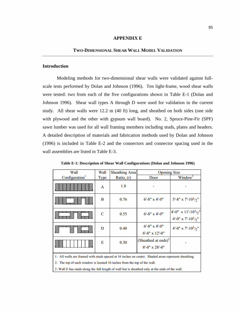
95
APPENDIX E
TWO-DIMENSIONAL SHEAR WALL MODEL VALIDATION
Introduction
Modeling methods for two-dimensional shear walls were validated against full-
scale tests performed by Dolan and Johnson (1996). Ten light-frame, wood shear walls
were tested: two from each of the five configurations shown in Table E-1 (Dolan and
Johnson 1996). Shear wall types A through D were used for validation in the current
study. All shear walls were 12.2 m (40 ft) long, and sheathed on both sides (one side
with plywood and the other with gypsum wall board). No. 2, Spruce-Pine-Fir (SPF)
sawn lumber was used for all wall framing members including studs, plates and headers.
A detailed description of materials and fabrication methods used by Dolan and Johnson
(1996) is included in Table E-2 and the connectors and connector spacing used in the
wall assemblies are listed in Table E-3.
Table E-1: Description of Shear Wall Configurations (Dolan and Johnson 1996)

96
Table E-2: Description of Materials and Construction Methods (Dolan and Johnson 1996)
Table E-3: Description of Connections used in Construction (Dolan and Johnson 1996)

97
The shear walls were tested horizontally, in-plane to the wall using the apparatus
shown in Figure E-1 (Dolan and Johnson 1996). The top and bottom chords of the walls
were anchored to steel tubes to prevent out-of-plane displacement during testing. A series
of increasing horizontal displacements were applied along the top chord of each wall,
representing increasing degrees of inter-story drift. The resultant force was then
measured and plotted against inter-story drift in a P-∆ plot. An “equivalent energy
elastic-plastic curve” was then developed for each wall configuration and used to
determine an equivalent elastic stiffness for each wall configuration (Dolan and Johnson
1996).
Figure E-1: Testing Apparatus and Sensor Locations (Dolan and Johnson 1996)
Modeling Methods
Framing Members
Studs, plates (top and bottom) and headers were modeled using SAP2000’s frame
elements. Opening headers constructed by Dolan and Johnson (1996) consisted of two
pieces of dimension lumber with an intermediate layer of plywood. To simplify the
modeling process, headers in the model were represented as one framing element with a
cross section equal to the total cross section of the header assembly and material
properties for the sawn lumber only. Table E-4 lists the frame element sections used in
the SAP2000 model.

98
Table E-4: Frame Sections Used for Modeling in SAP2000 – modeled through center of cross-section unless otherwise noted
Name of Frame Section Cross Section Dimensions
2x4 header 89 x 89 mm (3.5 x 3.5 in) 2x8 header 89 x 184 mm (3.5 x 7.25 in) 2x12 header 286 x 89 mm (3.5 x 11.25 in) Single Stud 38 x 89 mm (1.5 x 3.5 in)
Double Stud/Single Jack 76 x 89 mm (3.0 x 3.5 in) Double Jack 76 x 89 mm (4.5 x 3.5 in)
Double Top Plate 89 x 76 mm (3.5 x 3 in) (modeled through top of section)
Bottom Plate 89 x 38 mm (3.5 x 1.5 in) (modeled through bottom of section)
Figures E-2 and E-3 show an example of the framing layout for the wall Type D model.
All frame elements were assigned linear, isotropic material properties. A modulus of
elasticity (MOE) of 9653 MPa (1400 ksi) was determined from AF&PA (2005a) Table
4A for No. 2 SPF. No adjustment factors were used since the members were assumed to
be of normal moisture content (less than 19 percent), with no incisions and tested at
normal temperatures.
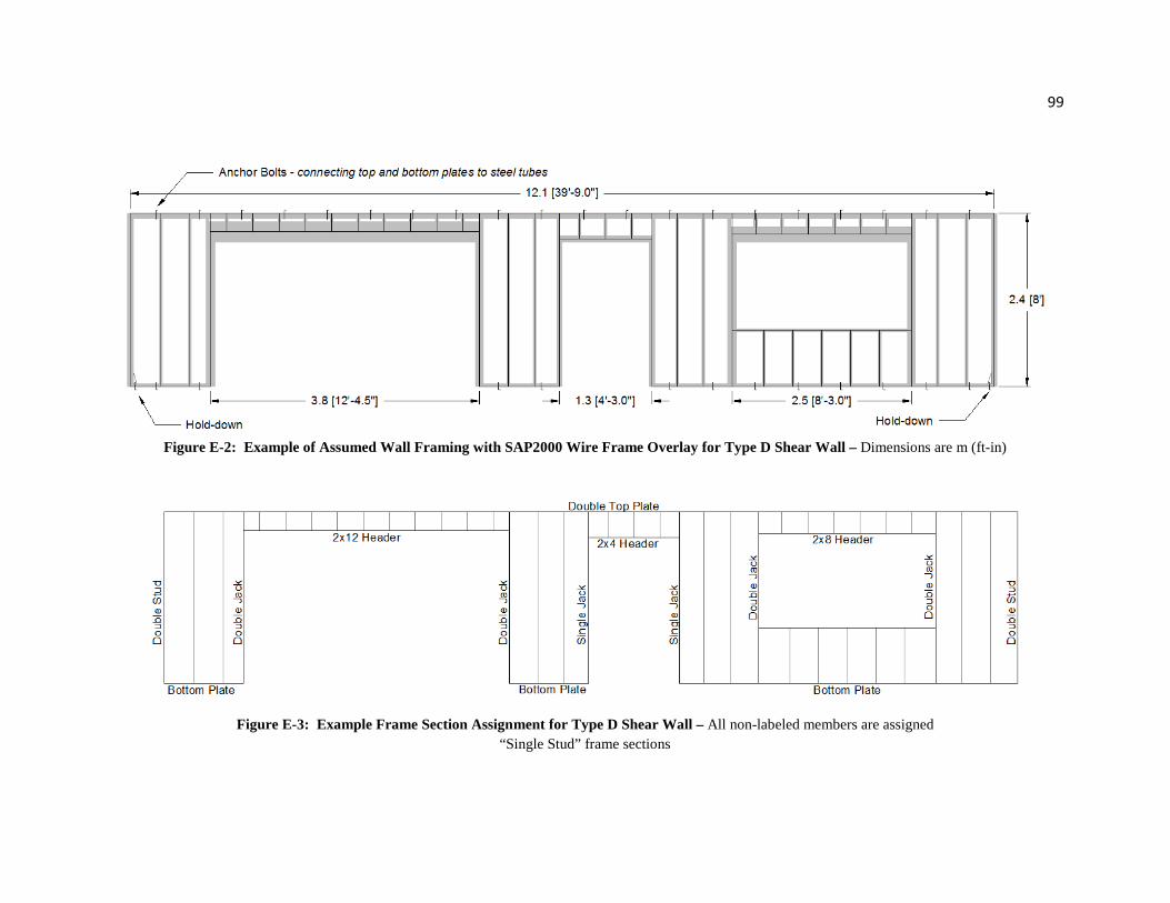
99
Figure E-2: Example of Assumed Wall Framing with SAP2000 Wire Frame Overlay for Type D Shear Wall – Dimensions are m (ft-in)
Figure E-3: Example Frame Section Assignment for Type D Shear Wall – All non-labeled members are assigned “Single Stud” frame sections

100
Plywood and Gypsum Wall Board Sheathing
Plywood and GWB sheathing were modeled using SAP2000’s layered shell
element as described in Table E-5 (with local axis 1 oriented parallel to the long side of
the plywood and local axis 3 oriented through the thickness of the plywood). The shell
element was modeled through the centerline of the wall with the plywood and GWB
layers displaced a distance of half the thickness of the wall framing members plus half
the thickness of the sheathing to either side of the wall centerline. In concurrence with
Martin (2010), one continuous shell element applied to each wall and meshed into
smaller, approximately square shaped elements for analysis.
Table E-5: Layered Shell Element Used for Modeling Sheathing in SAP2000
Layer Thickness Displacement (δ): from
centerline of wall to centerline of layer
Layer 1: Plywood Sheathing
11.9 mm (15/32 in)
50.4 mm (1.984 in)
Layer 2: Gypsum Wall
Board
12.7 mm (1/2 in)
50.8 mm (2 in)
Linear, orthotropic material properties for the plywood sheathing were determined
using the in-plane engineering properties from OSULaminates with the following inputs:
• Number of Plies = 4
• Ply Thickness = 3.97 mm (0.156 in)
• Ply Orientation = 0º - 90º - 90º - 0º
• Plywood Species Group 1
The gypsum wallboard was assigned linear isotropic properties using the orthotropic
input in SAP2000 so that the shear modulus, G12 , could be adjusted freely to account for
edge nail spacing (discussed later in this appendix and in Appendix F). The modulus of
elasticity for the GWB was determined as the average of the stiffness range listed by the
δ1
δ2
Wall Centerline
Layer 1
Layer 2

101
Gypsum Association (2010). An value of 0.3 was used for Poisson’s ratio. Table E-6
contains a full list of material properties assigned to each sheathing layer.
Table E-6: Material Properties Used for Modeling in SAP2000
Sheathing Material Properties
Plywood Sheathing (In-Plane Properties)
• Orthotropic Properties • E1 = 5337 MPa (774 ksi) • E2 = 5337 MPa (774 ksi) • U12 = 0.021
Calculated using OSULaminates
• G12 = 147 MPa (21.3 ksi) See Appendix F
Gypsum Wall Board
• OrthotropicProperties • E1 = 1820 MPa (264 ksi) • E2 = 1820 MPa (264 ksi) • U12 = 0.3
Gypsum Association (2010)
• G12 = 641 MPa (9.3 ksi) See Appendix F
Connectivity and Anchorage
Simple pinned connections were used to connect all framing members so that the
assembly stiffness of each wall could be controlled using the shear modulus (G12) of each
sheathing layer. Overall wall assembly stiffness (based on edge nail spacing and wall
length) was predicted using shear wall deflection equations from AF&PA (2005b)
Special Design Provisions for Wind and Seismic. Values of G12 for each sheathing layer
were then adjusted to reflect the predicted wall stiffness through a procedure similar to
the sheathing correlation procedure developed by Martin (2010). The procedure used in
the current study is described in detail in Appendix F.
Anchor bolts and hold-downs were modeled using directional linear spring
elements. The anchor bolts were represented using three springs: one oriented in the Z-
direction (representing the axial stiffness of each bolt) and two oriented in the X- and Y-
directions (representing the shear stiffness of each bolt). Hold-down devices were
represented with only one spring oriented in the Z-direction. Figure E-4 illustrates the

102
local axes orientation used for each anchorage device (Martin 2010). Figure E-5 shows
the location of the anchor bolts and hold- downs in the model.
Figure E-4: Local Axes for Anchor Bolts and Hold-downs (Martin 2010)
Figure E-5: Anchor Bolt and Hold-Down Placement in SAP2000 Model
Stiffness properties for anchorage devices are listed in Table E-7. The axial stiffness for
the anchor bolts was determined experimentally by Seaders (2004) and incorporates
wood crushing as well as bolt elongation and slip. The shear stiffness was determined
using Equation E-1, below, taken from AF&PA (2005a) Section 10.3.6 for load/slip
modulus, γ (kips/in), of dowel type connectors with diameter, D (in).
𝛾𝛾 = 270000(𝐷𝐷1.5) Equation E-1
Anchor bolts representing attachment of top plate to steel tube (Figure-E-1)
Anchor bolts representing bottom plate attachments Hold-downs

103
The axial stiffness of the hold-down device was determined using the allowable tension
load and displacement at allowable tension load reported by Simpson Strong-Tie (2012b)
for an HTT5 hold down with 16d fasteners connected to SPF wood. The HTT5
connector is listed by Simpson Strong-Tie (2012a) as the recommended alternative to the
HTT22 since the HTT22 has been discontinued.
Table E-7: Properties for Wall Anchorage used for Modeling in SAP2000
Anchorage Device Stiffness Placement Shear Axial
Anchor Bolts 23.3 kN/mm (133 kip/in)*
6.1 kN/mm (35 kip/in)**
Spaced 0.6 m (2 ft) on center and within 0.3 m (1 ft) of wall
ends
Hold-Downs --- 5674 kN/m
(32.4 kip/in)***
One at each end of wall
*Calculated from AF&PA (2005a) Section 10.3.6 **From Seaders (2004) ***Simpson Strong-Tie (2012b)
Results and Discussion
The stiffness of each shear wall model was found by displacing the top plate of
the model 8 mm (0.32 in) and then summing the lateral reactions at the anchors along the
base of the wall. Since the SAP2000 models are linear, the stiffness of the walls remains
constant regardless of displacement. Table E-8 compares the stiffness of the SAP2000
wall models to the equivalent elastic stiffness experimentally determined by Dolan and
Johnson (1996). For all cases, the models were able to predict the experimental elastic
stiffness of the walls within 5 percent error. The models were also accurate in predicting
the reduction in stiffness due to the addition of openings.

104
Table E-8: Stiffness Comparison between the SAP2000 Models from the Current Study and Tests from Dolan and Johnson (1996)
Wall Type
Dolan and Johnson (1996) Current Study
% Difference
Equivalent Elastic
Stiffness kN/mm (kip/in)
% Stiffness Reduction from Type
A
Model Stiffness
kN/mm (kip/in)
% Stiffness Reduction
from Type A
A 11.1 (63.6) --- 11.6 (66.4) --- 4% B 7.6 (43.5) 32% 7.2 (41.3) 38% -5% C 3.8 (21.5) 66% 3.7 (21.2) 68% -1% D 3.3 (18.6) 71% 3.2 (18.1) 73% -3%
Conclusions
The modeling procedures used in this appendix to represent light-frame, wood
shear walls were accurate in predicting the behavior of two-dimensional shear walls with
various opening configurations. Based on the results described in this appendix, the
following shear wall modeling methods were adopted for use in the current study:
• Framing members were modeled using the SAP2000 frame element with cross
sections equal to either the actual cross section of the member or the sum of the
cross sections when multiple members are placed side by side (as in double top
plates or built-up headers).
• Isotropic material properties for the framing members were determined using
design properties listed in AF&PA (2005a).
• Plywood and GWB sheathing were represented using a layered shell element with
each layer displaced as shown in Table E-5.
• Orthotropic material properties for the plywood sheathing were determined using
in-plane engineering properties from OSULaminates.
• Isotropic material properties for the GWB sheathing were determined from
properties published by the Gypsum Association (2010) and inserted into the
model using orthotropic material assignments.

105
• The effects of edge nail spacing and wall length were incorporated by adjusting
the shear modulus (G12) for the plywood sheathing and GWB based on the
procedure described in Appendix F.
• Anchor bolts and hold-downs were modeled using directional linear spring
elements oriented as shown in Figure E-4.
• Anchor bolt axial stiffness was determined from the experimental results of
Seaders (2004) and shear stiffness was calculated from AF&PA (2005a).
• Hold-down stiffness was determined from publications provided by the
manufacture.

106
APPENDIX F
SHEATHING G12 ADJUSTMENT PROCEDURE FOR EDGE NAIL SPACING
The effects of edge nail spacing on shear wall stiffness were incorporated through
a procedure similar to that used by Martin (2010). The shear modulus (G12) of the
sheathing was adjusted in SAP2000 to control the stiffness of the shear wall. This was
done by equating the deflection of a simple “calibration model” in SAP2000 to an
expected deflection calculated using Equation C4.3.2-2 (Equation F-1, below) from
AF&PA (2005b). The deflection of the calibration model is controlled by altering the
G12 of the sheathing. Equation F-1 gives a linear approximation for shear wall
deflections based on “framing bending deflection, panel shear deflection, deflection from
nail slip, and deflection due to tie-down slip” (AF&PA 2005b). The effects of panel
shear and nail slip are incorporated into an apparent stiffness term, Ga. Values for Ga are
tabulated in AF&PA (2005b) based on sheathing material, framing lay-out and edge-nail
spacing.
𝛿𝛿𝐴𝐴𝐴𝐴&𝑃𝑃𝐴𝐴 = 8𝑣𝑣ℎ3
𝐸𝐸𝐴𝐴𝐸𝐸+ 𝑣𝑣ℎ
1000𝐺𝐺𝑎𝑎+ ℎ
𝐸𝐸∆𝑎𝑎 Equation F-1
Where: δAF&PA = Expected shear wall deflection (in) v = Induced unit shear (plf) h = Shear wall height (ft) E = Modulus of elasticity of end posts (psi) A = Area of end post cross-section (in2) b = Shear wall length (ft) Ga = Apparent shear wall shear stiffness (kips/in) Δa = Total vertical elongation of wall anchorage system (in)
The following is a step-by-step example for determining the value of G12 for the plywood
sheathing used on the shear walls in Appendix E:
Step 1: A simple calibration model was created in SAP2000 for a 12.2-m-long (40-ft-
long) shear wall sheathed on one side, only, with the plywood used in shear wall
validation (Appendix E). Section and material properties for the plywood are
listed in Tables E-5 and E-6. In place of anchor bolts and hold-downs, rigid
supports were used in the calibration model as shown in Figure F-1.
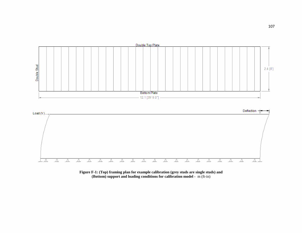
107
Figure F-1: (Top) framing plan for example calibration (grey studs are single studs) and (Bottom) support and loading conditions for calibration model - m (ft-in)

This was done so that the vertical elongation of wall anchorage, ∆a, in Equation
F-1 could be set equal to zero. The purpose of the calibration model is to
determine the required stiffness of the plywood sheathing for a specific edge
nail spacing and wall length. The effects of the anchor bolts and hold downs are
incorporated into the actual wall models later on by using linear springs with
realistic stiffness properties as explained in Appendix E and listed in Table E-7.
Step 2: A range of values for G12 of the plywood sheathing were entered into the
calibration model in SAP2000. For each value of G12, the deflection of the
model under an applied shear force, V, of 13.3 kN (3 kips) was recorded as
shown in Table F-1. G12 vs. deflection for the calibration model was then
plotted in Figure F-2, and fitted with a power curve described by Equation F-2.
Table F-1: Example of Shear Wall Deflections vs. Sheathing Shear Modulus, G12 in SAP2000
Plywood Sheathing Properties used in SAP2000 Wall Deflection at V = 13.3 kN (3 kips)
mm (in) E1
MPa (ksi) E2
MPa (ksi) Poisson’s Ratio, U12 G12 MPa (ksi)
5337 (774)
5337 (774) 0.021
414 (60) 0.356 (0.014) 276 (40) 0.584 (0.023) 138 (20) 1.295 (0.051) 69 (10) 2.743 (0.108)
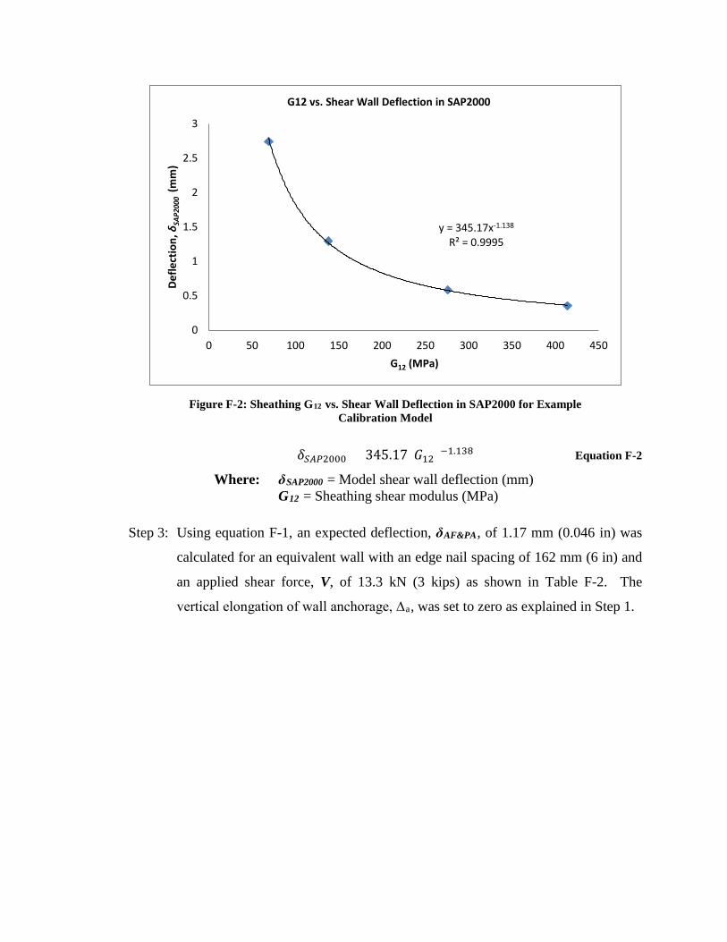
Figure F-2: Sheathing G12 vs. Shear Wall Deflection in SAP2000 for Example
Calibration Model
𝛿𝛿𝑆𝑆𝐴𝐴𝑃𝑃2000 = 345.17(𝐺𝐺12)−1.138 Equation F-2
Where: δSAP2000 = Model shear wall deflection (mm) G12 = Sheathing shear modulus (MPa)
Step 3: Using equation F-1, an expected deflection, δAF&PA, of 1.17 mm (0.046 in) was
calculated for an equivalent wall with an edge nail spacing of 162 mm (6 in) and
an applied shear force, V, of 13.3 kN (3 kips) as shown in Table F-2. The
vertical elongation of wall anchorage, ∆a, was set to zero as explained in Step 1.
y = 345.17x-1.138
R² = 0.9995
0
0.5
1
1.5
2
2.5
3
0 50 100 150 200 250 300 350 400 450
Defle
ctio
n, δ
SAP2
000
(mm
)
G12 (MPa)
G12 vs. Shear Wall Deflection in SAP2000

Table F-2: Example Shear Wall Deflection Calculation using Equation F-1 (AF&PA 2005b Equation C4.3.2-2) – in specified units
Edge Nail Spacing = 6 (in o.c.) Shear Wall Height (h) = 8 (ft) Shear Wall Length (b) = 40 (ft)
1Modulus of Elasticity of End Posts (E) = 1.4x10⁶ (psi) 2Area of End Post Cross-Section (A) = 10.5 (in2)
3Apparent Shear Wall Shear Stiffness (Ga) = 13.2 (kip/in) Total Vertical Elongation of Anchorage (Δa) = 0 (in)
4Force applied to top of wall = 3 (kips) Induced Unit Shear (v) = 75 (plf)
Calculated Deflection = 0.046 1.17
(in) (mm)
1AF&PA (2005a) Table 4A 2For two 38 x 89 mm (1.5 x 3.5 in) studs 3AF&PA (2005b) Table A.4.3A (increased by 1.2 for 4-ply sheathing per Table A.4.3A, Footnote 2) 4Chosen arbitrarily
Step 4: Finally, the required sheathing shear modulus, G12, was determined by equating
δSAP2000 in Equation F-2 to δAF&PA (converted to mm) calculated in step 3.
Solving for G12 gives a required shear modulus of 147 MPa (21.3) ksi for an
edge nail spacing of 162 mm (6 in). Repeating this method for several shear
walls of various lengths reveals that the required G12 for a specific edge nail
spacing changes approximately linearly with wall length as shown in Figure F-3.
Thus, for a building with multiple wall lengths and uniform edge nail spacing,
this procedure is only necessary for the shortest wall and the longest wall in the
building. Linear interpolation can be used for all other wall lengths.
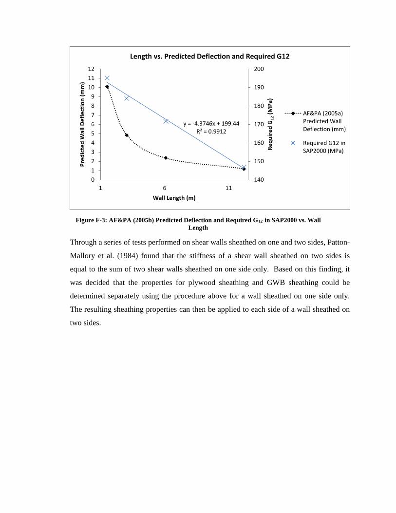
Figure F-3: AF&PA (2005b) Predicted Deflection and Required G12 in SAP2000 vs. Wall
Length
Through a series of tests performed on shear walls sheathed on one and two sides, Patton-
Mallory et al. (1984) found that the stiffness of a shear wall sheathed on two sides is
equal to the sum of two shear walls sheathed on one side only. Based on this finding, it
was decided that the properties for plywood sheathing and GWB sheathing could be
determined separately using the procedure above for a wall sheathed on one side only.
The resulting sheathing properties can then be applied to each side of a wall sheathed on
two sides.
y = -4.3746x + 199.44R² = 0.9912
140
150
160
170
180
190
200
0123456789
101112
1 6 11
Requ
ired
G12
(MPa
)
Pred
icte
d W
all D
efle
ctio
n (m
m)
Wall Length (m)
Length vs. Predicted Deflection and Required G12
AF&PA (2005a)Predicted WallDeflection (mm)
Required G12 inSAP2000 (MPa)

APPENDIX G
DETAILS FOR FULL BUILDING MODEL OF PAEVERE ET AL. (2003) HOUSE
The final validation study for the modeling methods described in this paper was
performed using the full-scale, realistic, L-shaped house tested by Paevere et al. (2003).
The full- scale house was designed jointly by the National Association of Home Builders
(NAHB) Research Center in the United States and the Commonwealth Scientific &
Industrial Research Organization (CSIRO) to reflect a typical North American “stick
frame” house (Paevere et al. 2003). Construction and testing of the house was done at the
CSIRO division of Building, Construction and Engineering testing facility in Melbourne,
Australia using equivalent Australian construction materials.
This Appendix contains construction and modeling details used for the Paevere et
al. (2003) house. Additional details for the house can be found in Paevere (2002). The
methods used to model the trusses, roof assemblies and wall assemblies are the same
methods described in detail in Appendices B through H. It is important to note the
following details:
• A modulus of elasticity of 10000 MPa (1450 ksi) given by Paevere (2002) was
used for the framing members in lieu of design properties from AF&PA (2005)
since radiata pine is not included in the AF&PA (2005a) NDS.
• The interior walls were modeled 25mm lower than the exterior walls so that the
roof trusses spanned the exterior walls only.
• Wall 3 was connected to the roof trusses using 2-joint link elements in SAP2000
to represent the slotted brackets used by Paevere (2002). Walls 6 and 8 were not
connected to the trusses.
• Wall corner framing was represented as one 90 x 90 mm (3.5 x 3.5 in) member to
simplify the modeling process.

Table G-1: Construction Details from Paevere (2002)
Wall Framing: Studs: 90x35 mm Machine Graded Pine (MGP) 10 spaced 400 mm on center without
blocking Bottom Plate: 90x45 mm MGP 10 Top Plate: double 90x35 mm MGP 10 Header Plate: 190x90 mm (short span) or 290x90 mm (long span) MOE: 10000 MPa (short duration) Average Density at 12% MC: 550 kg/m3
Bottom Plate Anchorage: Anchor Bolts: 12.7 mm bolts with plate washers spaced approximately 1000 mm
Roof Framing: Trusses: Pre-fabricated ‘gang-nailed’ pine trusses spaced 600 mm on center without
blocking Truss Connectors: Connected to top plate with pryda ‘triple-grip’ plate connectors Truss Top and Bottom Chords: 90x35 mm MGP 10 Truss Web Members: 70x35 mm MGP 10
Plywood Bracing: Walls: 2400x1200x9.5 mm F11 Bracing Ply (Laid Vertically) Roof: 2400x1200x12.5 mm F11 Ply (Laid Horizontally) Bending MOE: 10500 MPa
Gypsum Board Lining: 1200x2400x13 mm Gypsum Wall Board (Laid Horizontally)
Sheathing Nails: 2.87x50 mm machine driven nails spaced 150 mm on perimeter and 300 mm in field
Gypsum Board Lining: 6 gauge x 30 mm Needle-point Type 1 Gypsum Board Screws spaced 300 mm

Table G-2: Frame Sections Used in SAP2000 Model: Modeled through center of cross section unless otherwise noted.
Name of Frame Section Cross Section Dimensions
190x90 Header 190 x 90 mm (7.5 x 3.5 in) 290x90 Header 290 x 90 mm (11.4 x 3.5 in)
35x90 Header 35 x 90 mm (1.4 x 3.5 in) (used above doorways in interior walls)
290x90 Garage Beam 290 x 90 mm (11.4 x 3.5 in) (modeled through top of section)
Single Stud 35 x 90 mm (1.4 x 3.5 in) Double Stud 70 x 90 mm (2.8 x 3.5 in) Corner Stud 90 x 90 mm (3.5 x 3.5 in)
Double Top Plate 90 x 70 mm (3.5 x 2.8 in) (modeled through top of section)
Bottom Plate 90 x 45 mm (3.5 x 1.8 in) (modeled through bottom of section)
Truss Chord 35 x 90 mm (1.4 x 3.5 in) (modeled through bottom of section)
Truss Web 35 x 70 mm (1.4 x 2.8 in) (modeled through bottom of section)
Table G-3: Sheathing Material Properties used in SAP2000 Model
aPlywood Sheathing (for roof)
Orthotropic Properties • E1 = 8280 MPa (1201 ksi) • E2 = 2393 MPa (347 ksi) • U12 = 0.011 • G12 = 482 MPa (70 ksi)
From OSULaminates (Flexural Properties)
bPlywood Sheathing (for walls)
Orthotropic Properties • E1 = 7017 MPa (1018 ksi) • E2 = 3657 MPa (530 ksi) • U12 = 0.016 • G12 = See Figure G-1(a)
From OSULaminates (In-Plane Properties)
Gypsum Wall Board (for walls and ceiling)
Isotropic Properties • E1 = E2 = 1820 MPa (264
ksi) • U12 = 0.3 • G12 = See Figure G-1(b)
Gypsum Association (2010)
a. Assumed: 5-ply sheathing, 0⁰-90⁰-0⁰-90⁰-0⁰ ply orientation, species group 1 b. Assumed: 3-ply sheathing, 0⁰-90⁰-0⁰ ply orientation, species group 1
Table G-4: Properties for Wall Anchorage used for SAP2000 Model

Anchorage Device Stiffness Placement Sheara Axialb
Anchor Bolts 16.7 kN/mm (95.5 kip/in)
6.1 kN/mm (35 kip/in)
1.0 m (3.3 ft) maximum (See Figure G-2)
a. Calculated from AF&PA (2005a) Section 10.3.6 b. From Seaders (2004)
Table G-5: Material Densities used for Building Self-Weight
Material Density kg/m3 (pcf) Source
MGP 10 Framing Members 550 (1.07) Paevere (2002) F11 Plywood 600 (1.16) EWPAA (2009)
Gypsum Wall Board 772 (1.50) Gypsum Association (2010)
Figure G-1: G12 vs. Wall Length for 9.5 mm Plywood and 13 mm GWB Sheathing – Calculated using the procedure from Appendix F. Note: parameters for the GWB were
determined based on a fastener edge spacing of 200 mm (8 in) rather than 300 mm (12 in) since the latter is not included in AF&PA (2005b) Table 4.3B.
y = 24.013x - 0.4457
0
50
100
150
200
250
300
0 2 4 6 8 10 12
G12
(MPa
)
Wall Length (m)
9.5 mm Plywood Sheathing
y = -0.7247x + 50.742
0
50
100
150
200
250
300
0 2 4 6 8 10 12
G12
(MPa
)
Wall Length (m)
13 mm GWB Sheathing

Figure G-2: Anchor Bolt and Load Sensor Placement (Paevere 2002)
Figure G-3: Wall Locations Used in SAP2000 Model – m (ft-in)

Figure G-4: Wall Configurations (Paevere 2002) – Note: (1) The doorway in W3 was relocated as shown in Figure G-5 based on the point of intersection between W6 and W3.
(2) Interior walls were modeled 25 mm shorter than the exterior walls (Dr. Phillip Paevere, personal communication, June 25, 2012).
(see note 2, below)
(see note 1, below)
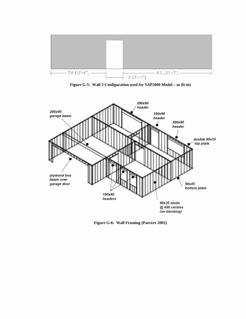
Figure G-5: Wall 3 Configuration used for SAP2000 Model – m (ft-in)
Figure G-6: Wall Framing (Paevere 2002)

Figure G-7: Example of Assumed Framing with SAP2000 Wire Frame Overlay for
Wall 2 – m (ft-in)
Figure G-8: Example Frame Section Assignment for Wall 2 – All connections are
pinned
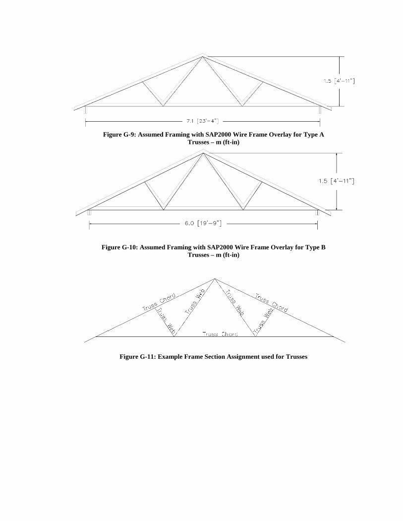
Figure G-9: Assumed Framing with SAP2000 Wire Frame Overlay for Type A
Trusses – m (ft-in)
Figure G-10: Assumed Framing with SAP2000 Wire Frame Overlay for Type B Trusses – m (ft-in)
Figure G-11: Example Frame Section Assignment used for Trusses

Figure G-12: Truss Layout for Type A and Type B Trusses
Figure G-13: 2-Joint Links used to Connect Wall 3 to Truss Bottom Chords – U2
(translation along the wall) is “fixed” for all links
2
1

Figure G-14: Gable-End Overhang Framing used in SAP2000 Model
Figure G-15: Gable-End Sheathing Placement used in SAP2000 Model

APPENDIX H
FULL BUILDING MODEL VALIDATION
Paevere et al. (2003) ran a series of static load tests on the full- scale house
described in Appendix G including:
• Gravity loads only (load case 1)
• Lateral point loads applied in N-S and E-W directions at various locations
along the top plates of the walls (load cases 2 through 12)
• Lateral point loads applied at various angles to the roof ridge above wall 5
(load cases 13 through 15)
This appendix contains plots comparing the load distributions in the house tested by
Paevere et al. (2003) to the SAP2000 model from the current study for load cases 2
through 15. The load distributions were determined by summing the reactions in the
direction parallel to the applied loads at the anchor bolts underneath the in-plane walls.
For load cases 13 through 15, where the load is applied at an angle, the load vector was
factored into N-S and E-W components applied simultaneously at the ridge.
In Load Case 1 (gravity only loads), Paevere (2002) noted that several load cells
were showing negative (uplift) reactions likely due to residual stresses from construction
(Paevere (2002). Consequenly, the load distribution to individual walls for Load Case 1
was not considered for this validation. The total self weight of the model was 55.7 kN,
which is 9.6% larger than the 50.8 kN reported by Paevere et al (2003). This
discrempancy could be due to the previously discussed uplift reactions seen in the tests,
differences in modeled and actual material densities and differences in over-framing used
to frame the roof above the garage. Details for the over-framing were not included in
Paevere et al. (2003). The load cells were zeroed for Load Cases 2 through 15 to negate
the effects of self weight, therefore the self weight of the model was also set to zero for
these cases.

Load Case 2: Wall 1 Loaded
Figure H-1: Load Case 2 – 2.78 kN Applied to Top-Plate at Wall 1
Figure H-2: Lateral Load Distribution to E-W Walls (Load Case 2)
0.0
2.0
4.0
6.0
8.0
10.0
12.0
14.0
Wall 1 Wall 2 Wall 3 Wall 4
Reac
tion
(kN
)
Lateral Load Distribution to E-W Walls
Paevere et al. (2003)
Current Study
2.78 kN

Load Case 3: Wall 2 Loaded
Figure H-3: Load Case 3 – 4.79 kN Applied to Top-Plate at Wall 2
Figure H-4: Lateral Load Distribution to E-W Walls (Load Case 3)
0.0
2.0
4.0
6.0
8.0
10.0
12.0
14.0
Wall 1 Wall 2 Wall 3 Wall 4
Reac
tion
(kN
)
Lateral Load Distribution to E-W Walls
Paevere et al. (2003)
Current Study
4.79 kN
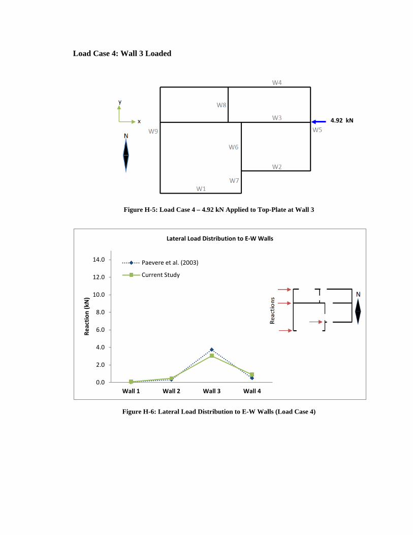
Load Case 4: Wall 3 Loaded
Figure H-5: Load Case 4 – 4.92 kN Applied to Top-Plate at Wall 3
Figure H-6: Lateral Load Distribution to E-W Walls (Load Case 4)
0.0
2.0
4.0
6.0
8.0
10.0
12.0
14.0
Wall 1 Wall 2 Wall 3 Wall 4
Reac
tion
(kN
)
Lateral Load Distribution to E-W Walls
Paevere et al. (2003)
Current Study
4.92 kN
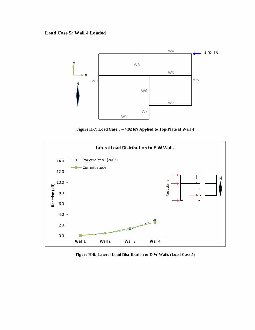
Load Case 5: Wall 4 Loaded
Figure H-7: Load Case 5 – 4.92 kN Applied to Top-Plate at Wall 4
Figure H-8: Lateral Load Distribution to E-W Walls (Load Case 5)
0.0
2.0
4.0
6.0
8.0
10.0
12.0
14.0
Wall 1 Wall 2 Wall 3 Wall 4
Reac
tion
(kN
)
Lateral Load Distribution to E-W Walls
Paevere et al. (2003)
Current Study
4.92 kN

Load Case 6: Wall 8 Loaded
Figure H-9: Load Case 6 – 5.18 kN Applied to Top-Plate at Wall 8
Figure H-10: Lateral Load Distribution to N-S Walls (Load Case 6)
0.0
2.0
4.0
6.0
8.0
10.0
12.0
14.0
Wall 9 Wall 6,7,8 Wall 5
Reac
tion
(kN
)
Lateral Load Distribution to N-S Walls
Paevere et al. (2003)
Current Study
5.18 kN

Load Case 7: Walls 2 and 8 Loaded
Figure H-11: Load Case 7 – 5.07 kN Applied to Top-Plate at Wall 2 and 5.13 kN Applied to Top-Plate at Wall 8
Figure H-12: Lateral Load Distribution to E-W Walls (Load Case 7)
-15.0
-13.0
-11.0
-9.0
-7.0
-5.0
-3.0
-1.0
Wall 1 Wall 2 Wall 3 Wall 4
Reac
tion
(kN
)
Lateral Load Distribution to E-W Walls
Paevere et al. (2003)
Current Study
5.13 kN
5.07 kN

Figure H-13: Lateral Load Distribution to N-S Walls (Load Case 7)
-2.0
0.0
2.0
4.0
6.0
8.0
10.0
12.0
Wall 9 Wall 6,7,8 Wall 5
Reac
tion
(kN
)
Lateral Load Distribution to N-S Walls
Paevere et al. (2003)
Current Study
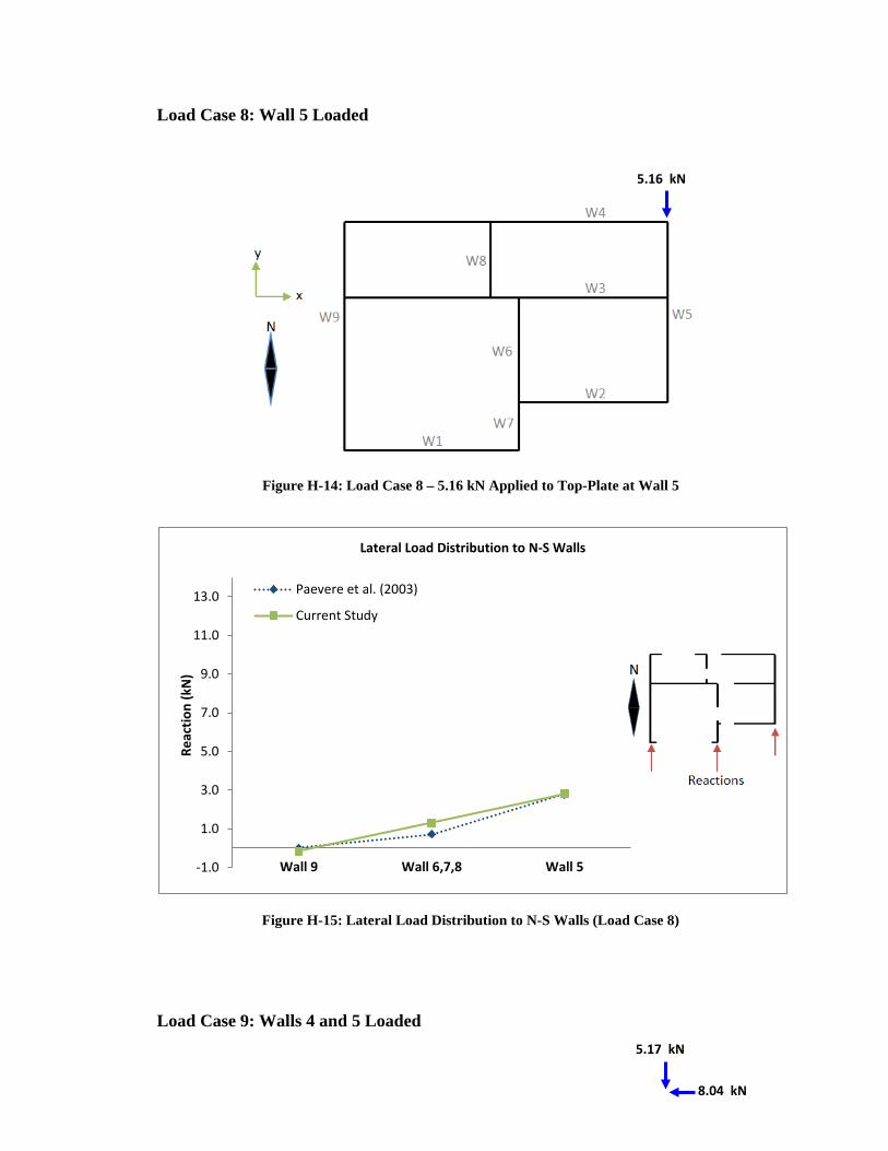
Load Case 8: Wall 5 Loaded
Figure H-14: Load Case 8 – 5.16 kN Applied to Top-Plate at Wall 5
Figure H-15: Lateral Load Distribution to N-S Walls (Load Case 8)
Load Case 9: Walls 4 and 5 Loaded
-1.0
1.0
3.0
5.0
7.0
9.0
11.0
13.0
Wall 9 Wall 6,7,8 Wall 5
Reac
tion
(kN
)
Lateral Load Distribution to N-S Walls
Paevere et al. (2003)
Current Study
5.16 kN
5.17 kN
8.04 kN

Figure H-16: Load Case 9 – 8.04 kN Applied to Top-Plate at Wall 4 and 5.17 kN Applied to Top-Plate at Wall 5
Figure H-17: Lateral Load Distribution to E-W Walls (Load Case 9)
-14.0
-12.0
-10.0
-8.0
-6.0
-4.0
-2.0
0.0
Wall 1 Wall 2 Wall 3 Wall 4
Reac
tion
(kN
)
Lateral Load Distribution to E-W Walls
Paevere et al. (2003)
Current Study

Figure H-18: Lateral Load Distribution to N-S Walls (Load Case 9)
-2.0
0.0
2.0
4.0
6.0
8.0
10.0
12.0
Wall 9 Wall 6,7,8 Wall 5
Reac
tion
(kN
)
Lateral Load Distribution to N-S Walls
Paevere et al. (2003)
Current Study

Load Case 10: Walls 2 and 5 Loaded
Figure H-19: Load Case 10 – 5.12 kN Applied to Top-Plate at Wall 2 and 3.18 kN Applied to Top-Plate at Wall 5
Figure H-20: Lateral Load Distribution to E-W Walls (Load Case 10)
-15.0
-13.0
-11.0
-9.0
-7.0
-5.0
-3.0
-1.0
Wall 1 Wall 2 Wall 3 Wall 4
Reac
tion
(kN
)
Lateral Load Distribution to E-W Walls
Paevere et al. (2003)
Current Study
3.18 kN
5.12 kN
Figure H-21: Lateral Load Distribution to N-S Walls (Load Case 10)
-1.0
1.0
3.0
5.0
7.0
9.0
11.0
13.0
Wall 9 Wall 6,7,8 Wall 5
Reac
tion
(kN
)
Lateral Load Distribution to N-S Walls
Paevere et al. (2003)
Current Study
Load Case 11: Load Applied between Walls 2 and 3
Figure H-22: Load Case 11 – 6.80 kN Applied to Top-Plate between Walls 2 and 3
Figure H-23: Lateral Load Distribution to E-W Walls (Load Case 11)
0.0
2.0
4.0
6.0
8.0
10.0
12.0
14.0
Walls 1 Walls 2 Walls 3 Walls 4
Reac
tion
(kN
)
Lateral Load Distribution to E-W Walls
Paevere et al. (2003)
Current Study
6.80 kN

Load Case 12: Load Applied to Walls 1, 2, 3 and 4
Figure H-24: Load Case 12 – 1.10 kN, 5.43 kN, 15.0 kN and 6.50 kN Applied to Top-Plate at Walls 1, 2, 3 and 4, respectively
Figure H-25: Lateral Load Distribution to E-W Walls (Load Case 12)
0.0
2.0
4.0
6.0
8.0
10.0
12.0
14.0
Wall 1 Wall 2 Wall 3 Wall 4
Reac
tion
(kN
)
Lateral Load Distribution to E-W Walls
Paevere et al. (2003)
Current Study
5.43 kN
1.10 kN
15.0 kN
6.50 kN
Load Case 13: Load Applied to Roof Ridge (at -5 degrees)
Figure H-26: Load Case 13 – 5.09 kN Applied to Roof Ridge of East Gable-End (at -5 degrees)
Figure H-27: Lateral Load Distribution to E-W Walls (Load Case 13)
-15.0
-13.0
-11.0
-9.0
-7.0
-5.0
-3.0
-1.0
Wall 1 Wall 2 Wall 3 Wall 4
Reac
tion
(kN
)
Lateral Load Distribution to E-W Walls
Paevere et al. (2003)
Current Study
5.09 kN
5⁰

Figure H-28: Lateral Load Distribution to N-S Walls (Load Case 13)
-1.0
1.0
3.0
5.0
7.0
9.0
11.0
13.0
Wall 9 Wall 6,7,8 Wall 5
Reac
tion
(kN
)
Lateral Load Distribution to N-S Walls
Paevere et al. (2003)
Current Study

Load Case 14: Load Applied to Roof Ridge (at -10 degrees)
Figure H-29: Load Case 14 – 5.21 kN Applied to Roof Ridge of East Gable-End (at -10 degrees)
Figure H-30: Lateral Load Distribution to E-W Walls (Load Case 14)
-15.0
-13.0
-11.0
-9.0
-7.0
-5.0
-3.0
-1.0
Wall 1 Wall 2 Wall 3 Wall 4
Reac
tion
(kN
)
Lateral Load Distribution to E-W Walls
Paevere et al. (2003)
Current Study
5.21 kN
10⁰

Figure H-31: Lateral Load Distribution to N-S Walls (Load Case 14)
-1.0
1.0
3.0
5.0
7.0
9.0
11.0
13.0
Wall 9 Wall 6,7,8 Wall 5
Reac
tion
(kN
)
Lateral Load Distribution to N-S Walls
Paevere et al. (2003)
Current Study

Load Case 15: Load Applied to Roof Ridge (at 20 degrees)
Figure H-32: Load Case 15 – 2.80 kN Applied to Roof Ridge of East Gable-End (at 20 degrees)
Figure H-33: Lateral Load Distribution to E-W Walls (Load Case 15)
-15.0
-13.0
-11.0
-9.0
-7.0
-5.0
-3.0
-1.0
Wall 1 Wall 2 Wall 3 Wall 4
Reac
tion
(kN
)
Lateral Load Distribution to E-W Walls
Paevere et al. (2003)
Current Study
2.80 kN
20⁰

Figure H-34: Lateral Load Distribution to N-S Walls (Load Case 15)
-2.0
0.0
2.0
4.0
6.0
8.0
10.0
12.0
Wall 9 Wall 6,7,8 Wall 5
Reac
tion
(kN
)
Lateral Load Distribution to N-S Walls
Paevere et al. (2003)
Current Study

APPENDIX I
MODEL VARIATIONS USED IN UPLIFT AND WIND LOAD INVESTIGATIONS
Using the validated modeling methods discussed in this study, multiple variations
of the Paevere et al (2003) house were created for use in uplift and lateral load path
investigations. All building variations were based on the same materials and construction
methods described in Appendix G, with the following modifications:
• Gable-end overhang framing was modified to reflect out-looker or out-
rigger style framing commonly used in North America as shown in Figure
I-1 (Martin 2010).
• Gable-end trusses were changed from Fink trusses to non-structural gable-
end frames and sheathed with plywood (Figure I-1).
• Simpson Strong-Tie HDU2 hold-downs (also used by Martin 2010) were
added to external walls at wall ends and at either side of openings. Hold-
downs were modeled with a stiffness of 6.1 kN/m (35 k/in) as listed by the
manufacturer (Martin 2010).
Wall designations used by Paevere et al. (2003) were also kept constant throughout the
load path investigations.
Two main investigations were performed: (1) an uplift investigation (2) a wind-
load (combined lateral and uplift) investigation. For each investigation, an index model
was created and systematically modified to explore the effects of geometric variations
and retrofits options. This appendix contains details for the buildings used in each
investigation. Further information including loading details and results from the
investigations are included in Appendices J through L.
Figure I-1: Gable End-Framing and Sheathing Modifications for Uplift and Wind Load Investigations
Uplift Investigation
Figure I-2: Progression of Building Variations Used in Uplift Investigation
Rectangular Index Building
L-Shaped Index Building
Opening Investigation
Opening in Wall 2
Addition of GWB on Ceiling and Walls
Opening in Wall 4 Opening in Wall 9 (Centered Under
Gable-End)
Opening in Wall 9 (Opposite Re-
Entrant Corner)
Addition of GWB on Ceiling and Walls
Addition of GWB on Ceiling
and Walls
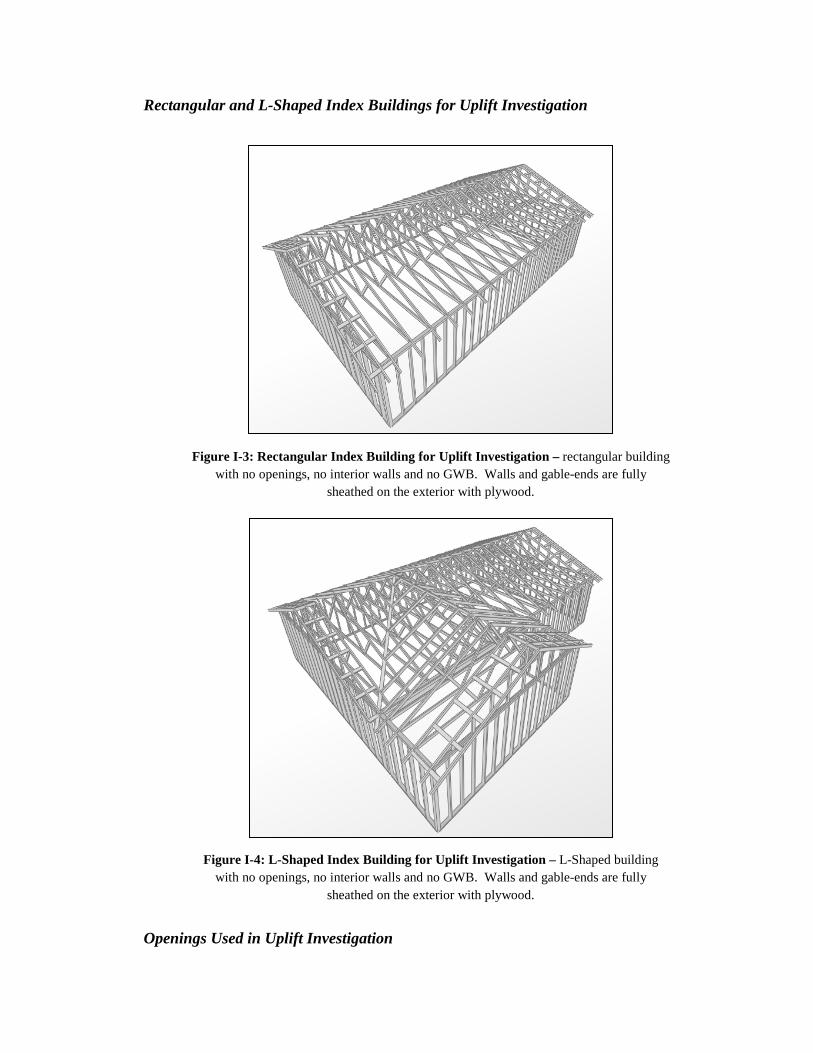
Rectangular and L-Shaped Index Buildings for Uplift Investigation
Figure I-3: Rectangular Index Building for Uplift Investigation – rectangular building
with no openings, no interior walls and no GWB. Walls and gable-ends are fully sheathed on the exterior with plywood.
Figure I-4: L-Shaped Index Building for Uplift Investigation – L-Shaped building
with no openings, no interior walls and no GWB. Walls and gable-ends are fully sheathed on the exterior with plywood.
Openings Used in Uplift Investigation

Figure I-5: Framing Detail for Openings used in Uplift Investigation
Figure I-6: Locations of Openings Used for Uplift Investigation
Wind Load Investigation
Opening in Wall 4 Opening in Wall 2
Opening in Wall 9 Centered Under
Gable-End
Opening in Wall 9 Opposite Re-Entrant
Corner
x
y
N
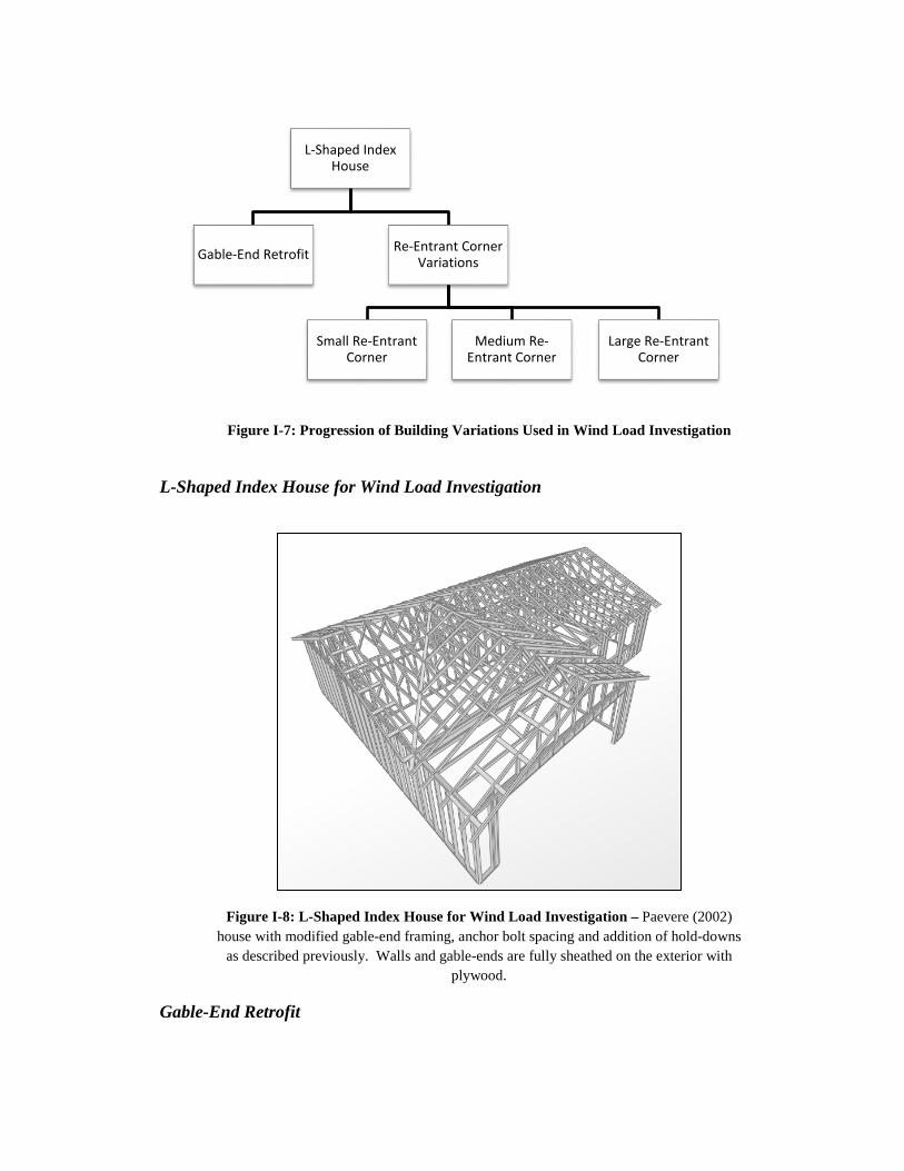
Figure I-7: Progression of Building Variations Used in Wind Load Investigation
L-Shaped Index House for Wind Load Investigation
Figure I-8: L-Shaped Index House for Wind Load Investigation – Paevere (2002)
house with modified gable-end framing, anchor bolt spacing and addition of hold-downs as described previously. Walls and gable-ends are fully sheathed on the exterior with
plywood.
Gable-End Retrofit
L-Shaped Index House
Gable-End Retrofit Re-Entrant Corner Variations
Small Re-Entrant Corner
Medium Re-Entrant Corner
Large Re-Entrant Corner

Figure I-9: Gable-End Retrofit Detail from 2010 Florida Building Code (ICC 2011)
Figure I-10: Gable-End Studs + Retrofit Studs Modeled with L-Shaped Cross-
Section

Figure I-11: Example of Gable-End Retrofit in the Model – Retrofits are located at
every gable-end stud. Retrofit connections are modeled as rigid connections.
Re-Entrant Corner Variations Used in Wind Load Investigation
Figure I-12: Re-Entrant Corner Variations Used in Wind Load Investigation – Small re-entrant corner (top left), index (top right), medium (bottom left) and large (bottom right)

Figure I-13: Re-Entrant Corner Variation Dimensions for Wind Load Investigation – m (ft-in)
x
y
N

APPENDIX J
UNIFORM UPLIFT INVESTIGATION
As a continuation of the research performed by Martin (2010), the propagation
and redistribution of uplift load paths due to changes in plan geometry and the addition of
openings in a simple light-frame, wood structure were investigated. Model variations
used in this study are described in detail in Appendix I and include:
• A rectangular index building with no interior walls, no wall openings and no
gypsum wall board lining.
• An L-shaped index building with no interior walls, no wall openings and no
gypsum wall board lining.
• Variations of the L-shaped building with openings added one at a time to each
of four locations as shown in Figure I-6.
• L-shaped index building with the addition of GWB on the ceiling and on the
interior of the walls.
• Two of the wall-opening variations with the addition of GWB on the ceiling
and on the interior of the walls.
In concurrence with Martin (2010), a uniform uplift pressure of 2.4 kPa (50 psf) was
applied to the roof of the buildings, normal to the surface. The self-weight of the
buildings was not included in the uplift investigation (Martin 2010). Resulting reactions
and changes in reaction for each building variation are included as “bubble plots” in this
appendix. Each bubble represents an individual hold-down or anchor bolt. The size of
the bubbles represents the magnitude of either the uplift reaction or change in reaction at
each anchorage device.
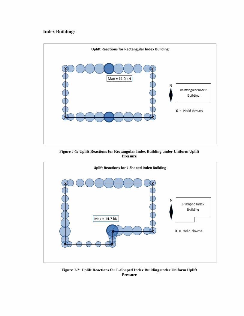
Index Buildings
Figure J-1: Uplift Reactions for Rectangular Index Building under Uniform Uplift Pressure
Figure J-2: Uplift Reactions for L-Shaped Index Building under Uniform Uplift Pressure
Max = 11.0 kN
Uplift Reactions for Rectangular Index Building
N
Max = 14.7 kN
Uplift Reactions for L-Shaped Index Building
N

Figure J-3: Difference in Uplift Reactions between Rectangular and L-Shaped Index Buildings under Uniform Uplift Pressure
Max ∆ = 8.3 kN
Difference from Rectangular Index Building(Magnified 4x)
N

Opening Investigation
L-Shaped Building with Opening in Wall 2
Figure J-4: Uplift Reactions for L-Shaped Building with Opening in Wall 2 (under
Uniform Uplift Pressure)
Figure J-5: Difference in Uplift Reactions due to Opening in Wall 2
Max = 18.2 kN
Uplift Reactions for L-Shaped Building with Opening in Wall 2
N
Max ∆ = 6.9 kN
Difference in Uplift Reactions from L-Shaped Index Building(Magnified 4x)
N
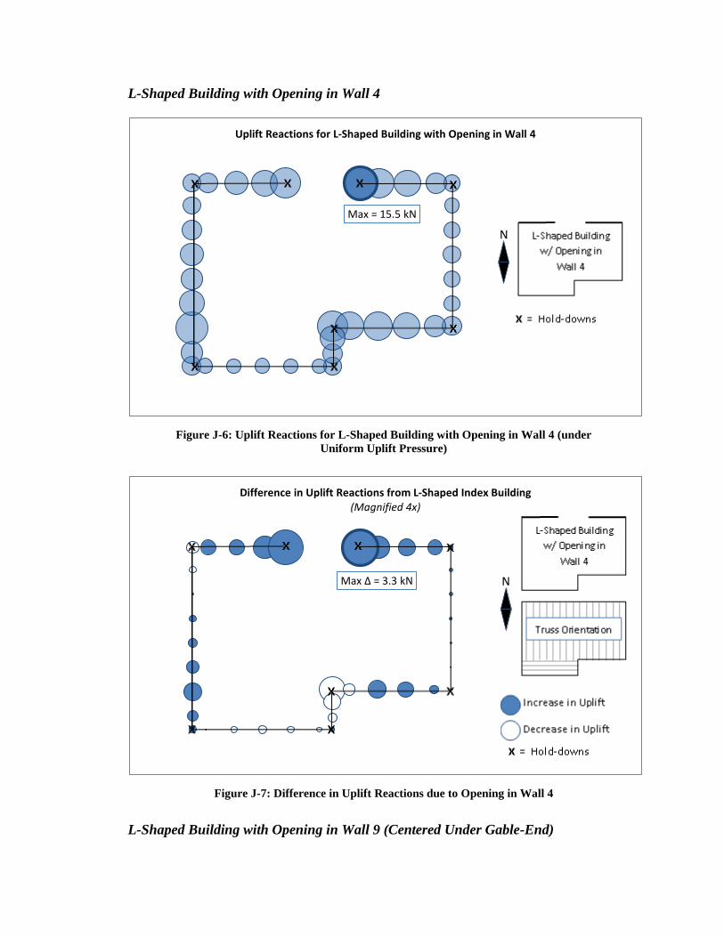
L-Shaped Building with Opening in Wall 4
Figure J-6: Uplift Reactions for L-Shaped Building with Opening in Wall 4 (under
Uniform Uplift Pressure)
Figure J-7: Difference in Uplift Reactions due to Opening in Wall 4
L-Shaped Building with Opening in Wall 9 (Centered Under Gable-End)
Max = 15.5 kN
Uplift Reactions for L-Shaped Building with Opening in Wall 4
N
Max ∆ = 3.3 kN
Difference in Uplift Reactions from L-Shaped Index Building(Magnified 4x)
N

Figure J-8: Uplift Reactions for L-Shaped Building with Opening in Wall 9,
Centered Under Gable-End (under Uniform Uplift Pressure)
Figure J-9: Difference in Uplift Reactions due to Opening in Wall 9, Centered Under Gable-End
L-Shaped Building with Opening in Wall 9 (Opposite Re-Entrant Corner)
Max = 14.7 kN
Uplift Reactions for L-Shaped Building with Opening in Wall 9(Centered Under Gable-End)
N
Max ∆ = 2.0 kN
Difference in Uplift Reactions from L-Shaped Index Building(Magnified 4x)
N

Figure J-10: Uplift Reactions for L-Shaped Building with Opening in Wall 9,
Opposite Re-Entrant Corner (under Uniform Uplift Pressure)
Figure J-11: Difference in Uplift Reactions due to Opening in Wall 9, Opposite Re-Entrant Corner
Effects of Gypsum Wall Board (GWB)
Max = 12.6 kN
Uplift Reactions for L-Shaped Building Opening in Wall 9(Opposite Re-Entrant Corner)
N
Max ∆ = 5.4 kN
Difference in Uplift Reactions from L-Shaped Index Building(Magnified 4x)
N

L-Shaped Building with GWB
Figure J-12: Uplift Reactions for L-Shaped Building with GWB (under Uniform Uplift Pressure)
Figure J-13: Difference in Uplift Reactions from L-Shaped Building due to addition of GWB
L-Shaped Building with Opening in Wall 2 and GWB
Max = 13.6 kN
Uplift Reactions for L-Shaped Building with GWB
N
Max ∆ = 1.2 kN
Difference in Uplift Reactions from L-Shaped Index Building due to Addition of GWB
(Magnified 4x)
N
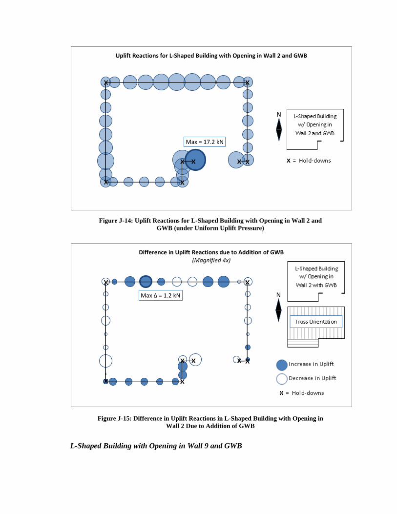
Figure J-14: Uplift Reactions for L-Shaped Building with Opening in Wall 2 and GWB (under Uniform Uplift Pressure)
Figure J-15: Difference in Uplift Reactions in L-Shaped Building with Opening in Wall 2 Due to Addition of GWB
L-Shaped Building with Opening in Wall 9 and GWB
Max = 17.2 kN
Uplift Reactions for L-Shaped Building with Opening in Wall 2 and GWB
N
Max ∆ = 1.2 kN
Difference in Uplift Reactions due to Addition of GWB(Magnified 4x)
N

Figure J-16: Uplift Reactions for L-Shaped Building with Opening in Wall 9 and GWB (under Uniform Uplift Pressure)
Figure J-17: Difference in Uplift Reactions in L-Shaped Building with Opening in Wall 9 Due to Addition of GWB
Max = 12.1 kN
Uplift Reactions for L-Shaped Building Opening in Wall 9(Opposite Re-Entrant Corner)
N
Max ∆ = 1.3 kN
Difference in Uplift Reactions from L-Shaped Index Building(Magnified 4x)
N

APPENDIX K
ASCE 7-05 DESIGN LOADS USED FOR WIND LOAD INVESTIGATION
Design wind loads for the wind load investigation were calculated using ASCE 7-
05 Main Wind Force Resisting System (MWFRS) Method 2 following methods outlined
in Mehta and Coulbourne (2010) Example 3.9. Three main wind directions were
considered: North-South, West-East and Southeast-Northwest as shown in Figure K-1.
ASCE 7-05 Wind Loads for MWFRS Method 2, Case 1 was used for the North-South
and West-East wind directions and Case 3 was used for the Southeast-Northwest wind
direction (Figure K-2).
Figure K-1: Wind Directions Considered for Wind Load Investigation
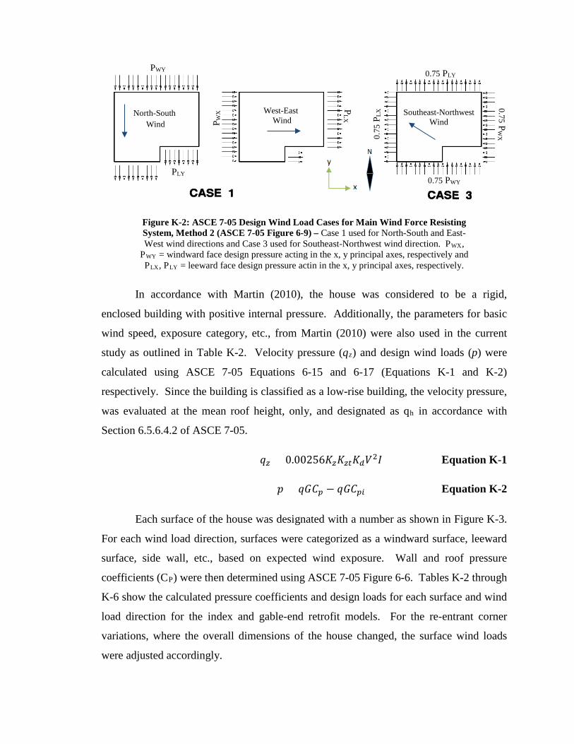
Figure K-2: ASCE 7-05 Design Wind Load Cases for Main Wind Force Resisting System, Method 2 (ASCE 7-05 Figure 6-9) – Case 1 used for North-South and East-West wind directions and Case 3 used for Southeast-Northwest wind direction. PWX,
PWY = windward face design pressure acting in the x, y principal axes, respectively and PLX, PLY = leeward face design pressure actin in the x, y principal axes, respectively.
In accordance with Martin (2010), the house was considered to be a rigid,
enclosed building with positive internal pressure. Additionally, the parameters for basic
wind speed, exposure category, etc., from Martin (2010) were also used in the current
study as outlined in Table K-2. Velocity pressure (qz) and design wind loads (p) were
calculated using ASCE 7-05 Equations 6-15 and 6-17 (Equations K-1 and K-2)
respectively. Since the building is classified as a low-rise building, the velocity pressure,
was evaluated at the mean roof height, only, and designated as qh in accordance with
Section 6.5.6.4.2 of ASCE 7-05.
𝑞𝑞𝑧𝑧 = 0.00256𝐾𝐾𝑧𝑧𝐾𝐾𝑧𝑧𝑧𝑧𝐾𝐾𝑑𝑑𝑉𝑉2𝐼𝐼 Equation K-1
𝑝𝑝 = 𝑞𝑞𝐺𝐺𝐶𝐶𝑝𝑝 − 𝑞𝑞𝐺𝐺𝐶𝐶𝑝𝑝𝑝𝑝 Equation K-2
Each surface of the house was designated with a number as shown in Figure K-3.
For each wind load direction, surfaces were categorized as a windward surface, leeward
surface, side wall, etc., based on expected wind exposure. Wall and roof pressure
coefficients (CP) were then determined using ASCE 7-05 Figure 6-6. Tables K-2 through
K-6 show the calculated pressure coefficients and design loads for each surface and wind
load direction for the index and gable-end retrofit models. For the re-entrant corner
variations, where the overall dimensions of the house changed, the surface wind loads
were adjusted accordingly.
North-South Wind
West-East Wind
Southeast-Northwest Wind
PLY 0.75 PWY
PWY 0.75 PLY
P WX
0.75 PW
X 0.
75 P
LX P
LX

Figure K-3: Surface Designations used for Wind Pressure Calculations
Table K-1: Parameters used for ASCE 7-05 MWFRS Design Wind Loads Method 2 – Given in specified units for ASCE 7-05 Equation 6-15
Exposure Category = B Martin (2010)
Occupancy Category = II Martin (2010)
Building Type = Low-rise, enclosed Basic Wind Speed (V) = 130 mph Martin (2010)
Wind Directionality Factor (Kd) = 0.85 ASCE 7-05 Table 6-4
Importance Factor (I) = 1 Martin (2010)
Topographic Factor (Kzt) = 1 Martin (2010) Internal Pressure Coefficient
(GCpi) = (+) 0.18 ASCE 7-05 Figure 6-5
Gust Factor (G) = 0.85 ASCE 7-05 6.5.8.1 - Rigid Structure Mean Roof Height (h) = 10.35 ft
Exposure Category (Kz) = Kh = 0.57 ASCE 7-05 Table 6-3 Velocity Pressure (qz) = qh = 20.96 psf ASCE 7-05 Equation 6-15

Table K-2: Design Pressures for Index House under North-South Wind ASCE 7-05 Load Case 1 (Figure K-2)
Surface Type Designation (Figure K-3)
Cp (ASCE 7-05 Figure
6-6)
External Pressure qGCp Pa
(psf)
(+) Internal Pressure
qh(GCpi) Pa (psf)
Net Pressure, p Pa (psf)
Windward Wall 6 0.8 685 (14.3) 182 (3.8) 503 (10.5) Overhanga 6 0.8 685 (14.3) 0 685 (14.3) Side Wall 1,3,5 -0.7 -599 (-12.5) 182 (3.8) -776 (-16.2)
Leeward Wallb 2,4 -0.5 -426 (-8.9) 182 (3.8) -608 (-12.7) Windward Roofc 7 -0.28 -239 (-5.0) 182 (3.8) -421 (-8.8)
Leeward Roof 8,9,10,11 -0.6 -512 (-10.7) 182 (3.8) -694 (-14.5) a. Cp = 0.8 (ASCE 7-05 Section 6.5.11.4.1) b. For L/B = 0.82 c. Interpolated for θ = 23⁰ and h/L = 0.35
Table K-3: Design Pressures for Index House under West-East Wind
ASCE 7-05 Load Case 1 (Figure K-2)
Surface Type Designation (Figure K-3)
Cp (ASCE 7-05 Figure
6-6)
External Pressure
qGCp Pa (psf)
(+) Internal Pressure qh(GCpi) Pa (psf)
Net Pressure, p
Pa (psf)
Windward Wall 1 0.8 685 (14.3) 182 (3.8) 503 (10.5) Overhanga 1 0.8 685 (14.3) 0 685 (14.3) Side Wall 2,4,6 -0.7 -599 (-12.5) 182 (3.8) -776 (-16.2)
Leeward Wallb 3,5 -0.46 -393 (-8.2) 182 (3.8) -575 (-12.0) Windward Roofc 9 -0.21 -177 (-3.7) 182 (3.8) -359 (-7.5)
Leeward Roof 10,11 -0.6 -512 (-10.7) 182 (3.8) -694 (-14.5) Roof // to Ridge
0 to 1.6 m 7,8 -0.9 -766 (-16.0) 182 (3.8) -948 (-19.8) 1.6 m to 3.1 m 7,8 -0.9 -766 (-16) 182 (3.8) -948 (-19.8) 3.1 m to 6.3 m 7,8 -0.5 -426 (8.9) 182 (3.8) -608 (-12.7)
> 6.3 m 7,8 -0.3 -254 (-5.3) 182 (3.8) -436 (-9.1) a. Cp = 0.8 (ASCE 7-05 Section 6.5.11.4.1) b. For L/B = 1.2 c. Interpolated for θ = 26⁰ and h/L = 0.28

Table K-4: ASCE 7-05 Design Pressures for Index House under South-North Wind
Surface Type Designation (Figure K-3)
Cp (ASCE 7-05 Figure
6-6)
External Pressure qGCp Pa
(psf)
(+) Internal Pressure qh(GCpi) Pa (psf)
Net Pressure, p
Pa (psf)
Windward Wall 2,4 0.8 685 (14.3) 182 (3.8) 503 (10.5) Overhang 2,4 0.8 685 (14.3) 0 685 (14.3)
Leeward Wall 6 -0.5 -426 (8.9) 182 (3.8) -608 (-12.7) Windward Roof 8,11 -0.28 -239 (-5.0) 182 (3.8) -421 (-8.8) Leeward Roof 7 -0.6 -512 (-10.7) 182 (3.8) -694 (-14.5)
a. Cp = 0.8 (ASCE 7-05 Section 6.5.11.4.1) b. For L/B = 0.82 c. Interpolated for θ = 23⁰ and h/L = 0.35 Table K-5: ASCE 7-05 Design Pressures for Index House under East-West Wind
Surface Type Designation (Figure K-3)
Cp (ASCE 7-05 Figure
6-6)
External Pressure qGCp Pa
(psf)
(+) Internal Pressure qh(GCpi) Pa (psf)
Net Pressure, p Pa (psf)
Windward Wall 3,5 0.8 685 (14.3) 182 (3.8) 503 (10.5) Overhang 3,5 0.8 685 (14.3) 0 685 (14.3)
Leeward Wall 1 -0.46 -393 (-8.2) 182 (3.8) -575 (-12.0) Windward Roof 10 -0.21 -177 (-3.7) 182 (3.8) -359 (-7.5) Leeward Roof 9,8 -0.6 -512 (-10.7) 182 (3.8) -694 (-14.5)
a. Cp = 0.8 (ASCE 7-05 Section 6.5.11.4.1) b. For L/B = 1.2 c. Interpolated for θ = 26⁰ and h/L = 0.28

Table K-6: Design Pressures for Index Building under Southeast-Northwest Wind = 0.75(S-N) + 0.75(E-W) – ASCE 7-05 Load Case 3 (Figure K-2)
Surface Type Designation (Figure K-3)
S-N Net Pressure p
Pa (psf)
E-W Net Pressure p
Pa (psf) 0.75*p
Pa (psf)
Windward Wall 2,4 503 (10.5) 378 (7.9) Overhang 2,4 685 (14.3) 512 (10.7)
Windward Wall 5,3 503 (10.5) 378 (7.9) Overhang 5,3 685 (14.3) 512 (10.7)
Leeward Wall 6 -608 (-12.7) -455 (-9.5) Leeward Wall 1 -575 (-12.0) -431 (-9.0)
Windward Roof 11 -421 (-8.8) -316 (-6.6) Windward Roof 10 -359 (-7.5) -268 (-5.6) Leeward Roof 7 -694 (-14.5) -522 (-10.9) Leeward Roof 9,8 -694 (-14.5) -522 (-10.9)

APPENDIX L
WIND LOAD INVESTIGATION
For the wind load investigation, the propagation of lateral and uplift wind loads
through an L-shaped house were modeled and analyzed. The house was then
systematically modified to study the redistribution of wind loads due to the addition of a
gable-end retrofit and various re-entrant corner dimensions. Model variations used for
the wind load investigation are detailed in Appendix I and include:
• A model of the Paevere et al. (2003) house with the gable-end framing, hold-
down and sheathing modifications described in Appendix I. This building is
designated as the L-shaped index house for this investigation.
• The L-shaped index house with the addition of gable-end retrofits as
recommended in the 2010 Florida Building Code (Figure I-9).
• The L-shaped index house with one leg of the “L” shortened/extended as
shown in Figure I-13 to create three re-entrant corner variations:
o Small re-entrant corner (leg shortened by 1.2 m)
o Medium re-entrant corner (leg extended by 1.2 m)
o Large re-entrant corner (leg extended to create a re-entrant corner
with 1:1 dimensional ratio)
All model variations in this investigation include the self weight of the construction
materials for realistic results. Models were loaded with ASCE 7-05 design wind loads for
each of the three wind directions described in Appendix K. Uplift and change in uplift
reactions for each building were plotted using the same “bubble plots” used in Appendix
J. Lateral load distributions to in-plane walls were also plotted for each model and load
case.

L-shaped index house
North to South Wind Loads
Figure L-1: Uplift Reactions for L-shaped index house under North-South Wind
Loads (with Self Weight)
Figure L-2: Lateral Load Distribution to North-South walls under North-South
Wind Loads (with Self Weight)
West to East Wind Loads
Max = 1.4 kN
Uplift Reactions - with Self Weight
N
0
1
2
3
4
5
6
7
8
9
10
Wall 9 Wall 6,7,8 Wall 5
Reac
tion
(kN
)
Lateral Load Distribution to N-S Walls
N

Figure L-3: Uplift Reactions for L-shaped index house under West-East Wind
Loads (with Self Weight)
Figure L-4: Lateral Load Distribution to East-West walls under West-East Wind Loads (with Self Weight)
Southeast-Northwest Wind Loads
Max = 3.1 kN
Uplift Reactions - with Self Weight
N
0
1
2
3
4
5
6
7
8
9
10
Wall 1 Wall 2 Wall 3 Wall 4
Reac
tion
(kN
)
Lateral Load Distribution to E-W Walls
N
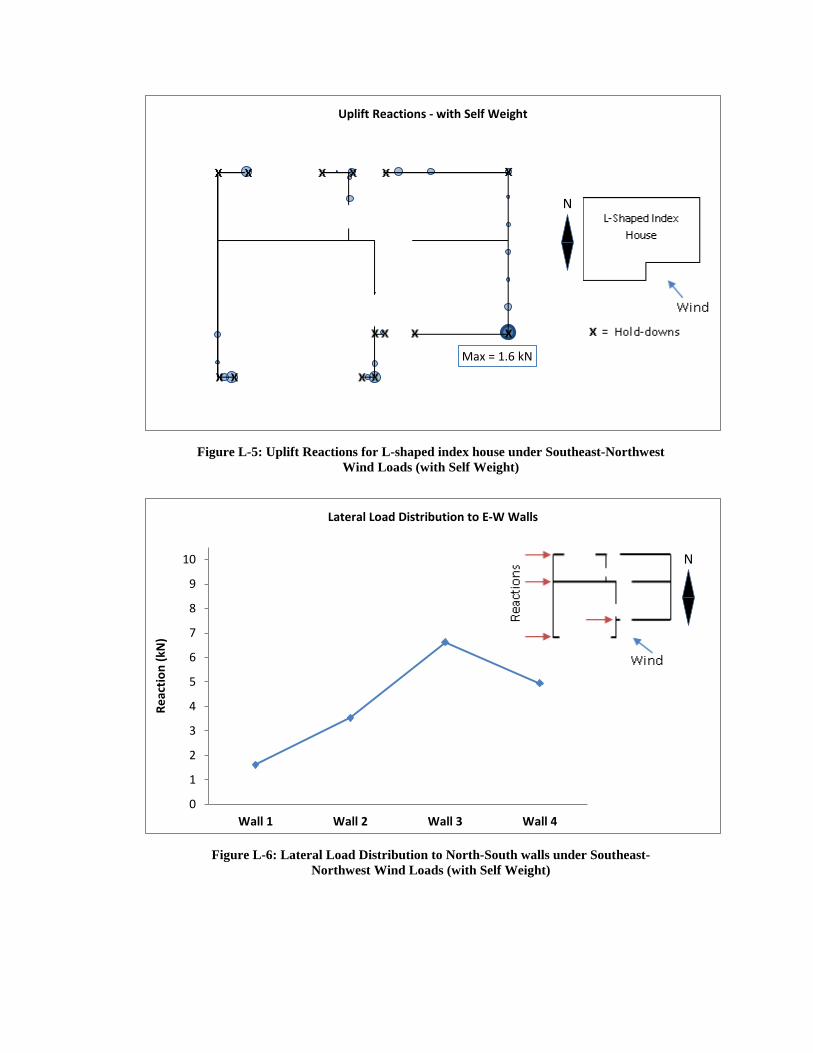
Figure L-5: Uplift Reactions for L-shaped index house under Southeast-Northwest
Wind Loads (with Self Weight)
Figure L-6: Lateral Load Distribution to North-South walls under Southeast-Northwest Wind Loads (with Self Weight)
Max = 1.6 kN
Uplift Reactions - with Self Weight
N
0
1
2
3
4
5
6
7
8
9
10
Wall 1 Wall 2 Wall 3 Wall 4
Reac
tion
(kN
)
Lateral Load Distribution to E-W Walls
N

Figure L-7: Lateral Load Distribution to East-West walls under Southeast-Northwest Wind Loads (with Self Weight)
0
1
2
3
4
5
6
7
8
9
10
Wall 9 Wall 6,7,8 Wall 5
Reac
tion
(kN
)
Lateral Load Distribution to N-S Walls
N

Gable-End Retrofit Investigation
North-South Wind Load
Figure L-8: Uplift Reactions for Building with Gable-End Retrofits under North-
South Wind Loads (with Self Weight)
Figure L-9: Difference in Uplift Reactions between Building with Gable-End
Retrofits and L-shaped index house under North-South Wind Loads (with Self Weight)
Max = 1.3 kN
Uplift Reactions - with Self Weight
N
Max = 0.19 kN
Difference in Uplift Reactions (from L-Shaped Index House) -with Self Weight
N
Magnified 4x

Figure L-10: Lateral Load Distribution to North-South walls under North-South
Wind Loads (with Self Weight)
0
1
2
3
4
5
6
7
8
9
10
Wall 9 Wall 6,7,8 Wall 5
Reac
tion
(kN
)
Lateral Load Distribution to N-S Walls
L-Shaped Index House
Gable-End Retrofit
N
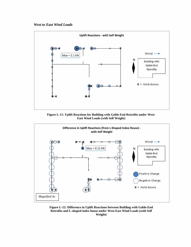
West to East Wind Loads
Figure L-11: Uplift Reactions for Building with Gable-End Retrofits under West-
East Wind Loads (with Self Weight)
Figure L-12: Difference in Uplift Reactions between Building with Gable-End Retrofits and L-shaped index house under West-East Wind Loads (with Self
Weight)
Max = 2.1 kN
Uplift Reactions - with Self Weight
N
Max = 0.12 kN
Difference in Uplift Reactions (from L-Shaped Index House) -with Self Weight
N
Magnified 4x

Figure L-13: Lateral Load Distribution to East-West walls under West-East Wind
Loads (with Self Weight)
0
1
2
3
4
5
6
7
8
9
10
Wall 1 Wall 2 Wall 3 Wall 4
Reac
tion
(kN
)
Lateral Load Distribution to E-W Walls
L-Shaped Index House
Gable-End Retrofit
N

Southeast to Northwest Wind Loads
Figure L-14: Uplift Reactions for Building with Gable-End Retrofits under
Southeast-Northwest Wind Loads (with Self Weight)
Figure L-15: Difference in Uplift Reactions between Building with Gable-End
Retrofits and L-shaped index house under Southeast-Northwest Wind Loads (with Self Weight)
Max = 1.2 kN
Uplift Reactions - with Self Weight
N
Max = 0.15 kN
Difference in Uplift Reactions (from L-Shaped Index House) -with Self Weight
N
Magnified 4x

Figure L-16: Lateral Load Distribution to East-West walls under Southeast-
Northwest Wind Loads (with Self Weight)
Figure L-17: Lateral Load Distribution to North-South walls under Southeast-
Northwest Wind Loads (with Self Weight)
Re-Entrant Corner Investigation
0
1
2
3
4
5
6
7
8
9
10
Wall 1 Wall 2 Wall 3 Wall 4
Reac
tion
(kN
)
Lateral Load Distribution to E-W Walls
L-Shaped Index House
Building with Gable-End Retrofit
N
0
1
2
3
4
5
6
7
8
9
10
Wall 9 Wall 6,7,8 Wall 5
Reac
tion
(kN
)
Lateral Load Distribution to N-S Walls
L-Shaped Index House
Building with Gable-End Retrofit
N

North to South Wind Loads
Figure L-18: Uplift Reactions for Building with Small Re-Entrant Corner under
North-South Wind Loads (with Self Weight)
Figure L-19: Difference in Uplift Reactions between Building with Small Re-Entrant
Corner and L-shaped index house under North-South Wind Loads (with Self Weight)
Max = 1.2 kN
Uplift Reactions for Small Re-Entrant Corner -with Self Weight
N
Max = 0.39 kN
Difference in Uplift Reactions (from L-Shaped Index House) -with Self Weight
N
Magnified 4x

Figure L-20: Uplift Reactions for Building with Medium Re-Entrant Corner under
North-South Wind Loads (with Self Weight)
Figure L-21: Difference in Uplift Reactions between Building with Medium Re-
Entrant Corner and L-shaped index house under North-South Wind Loads (with Self Weight)
Max = 1.5 kN
Uplift Reactions (Medium Re-Entrant Corner) -with Self Weight
N
Max = 0.27 kN
Difference in Uplift Reactions (from L-Shaped Index House) -with Self Weight
N
Magnified 4x

Figure L-22: Uplift Reactions for Building with Large Re-Entrant Corner under
North-South Wind Loads (with Self Weight)
Figure L-23: Difference in Uplift Reactions between Building with Large Re-
Entrant Corner and L-shaped index house under North-South Wind Loads (with Self Weight)
Max = 1.5 kN
Uplift Reactions (Large Re-Entrant Corner) -with Self Weight
N
Max = 0.83 kN
Difference in Uplift Reactions (from L-Shaped Index House) -with Self Weight
N
Magnified 4x

Figure L-24: Lateral Load Distribution to North-South walls under North-South
Wind Loads (with Self Weight)
Figure L-25: Unit Shear in North-South walls under North-South Wind Loads (with
Self Weight)
0
1
2
3
4
5
6
7
8
9
10
Wall 9 Wall 6,7,8 Wall 5
Reac
tion
(kN
)
Lateral Load Distribution to N-S Walls
Small Re-entrant CornerL-Shaped Index HouseMedium Re-entrant CornerLarge Re-entrant Corner
N
0
0.1
0.2
0.3
0.4
0.5
0.6
0.7
0.8
0.9
1
Wall 9 Wall 6,7,8 Wall 5
Uni
t She
ar (k
N/m
)
Unit Shear in N-S Walls
Small Re-entrant CornerL-Shaped Index HouseMedium Re-entrant CornerLarge Re-entrant Corner
N

West to East Wind Loads
Figure L-26: Uplift Reactions for Building with Small Re-Entrant Corner under
West-East Wind Loads (with Self Weight)
Figure L-27: Difference in Uplift Reactions between Building with Small Re-Entrant Corner and L-shaped index house under West-East Wind Loads (with Self Weight)
Max = 3.0 kN
Uplift Reactions (Small Re-Entrant Corner) -with Self Weight
N
Max = 0.59 kN
Difference in Uplift Reactions (from L-Shaped Index House) -with Self Weight
N
Magnified 4x

Figure L-28: Uplift Reactions for Building with Medium Re-Entrant Corner under
West-East Wind Loads (with Self Weight)
Figure L-29: Difference in Uplift Reactions between Building with Medium Re-
Entrant Corner and L-shaped index house under West-East Wind Loads (with Self Weight)
Max = 3.3 kN
Uplift Reactions (Medium Re-Entrant Corner) -with Self Weight
N
Max = 0.36 kN
Difference in Uplift Reactions (from L-Shaped Index House) -with Self Weight
N
Magnified 4x

Figure L-30: Uplift Reactions for Building with Large Re-Entrant Corner under
West-East Wind Loads (with Self Weight)
Figure L-31: Difference in Uplift Reactions between Building with Large Re-
Entrant Corner and L-shaped index house under West-East Wind Loads (with Self Weight)
Max = 3.5 kN
Uplift Reactions (Large Re-Entrant Corner) -with Self Weight
N
Max = 0.49 kN
Difference in Uplift Reactions (from L-Shaped Index House) -with Self Weight
N
Magnified 4x

Figure L-32: Lateral Load Distribution to East-West walls under West-East Wind
Loads (with Self Weight)
0
1
2
3
4
5
6
7
8
9
10
Wall 1 Wall 2 Wall 3 Wall 4
Reac
tion
(kN
)
Lateral Load Distribution to E-W Walls
Small Re-entrant CornerL-Shaped Index HouseMedium Re-entrant CornerLarge Re-entrant Corner
N
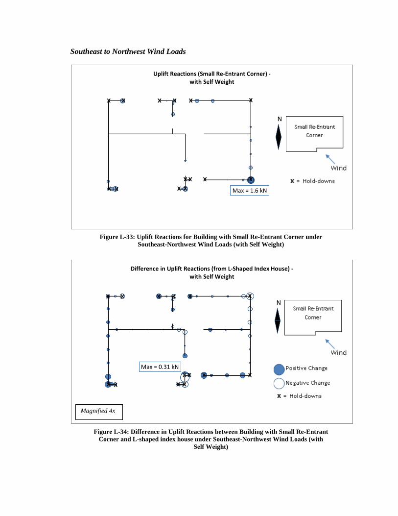
Southeast to Northwest Wind Loads
Figure L-33: Uplift Reactions for Building with Small Re-Entrant Corner under
Southeast-Northwest Wind Loads (with Self Weight)
Figure L-34: Difference in Uplift Reactions between Building with Small Re-Entrant
Corner and L-shaped index house under Southeast-Northwest Wind Loads (with Self Weight)
Max = 1.6 kN
Uplift Reactions (Small Re-Entrant Corner) -with Self Weight
N
Max = 0.31 kN
Difference in Uplift Reactions (from L-Shaped Index House) -with Self Weight
N
Magnified 4x

Figure L-35: Uplift Reactions for Building with Medium Re-Entrant Corner under
Southeast-Northwest Wind Loads (with Self Weight)
Figure L-36: Difference in Uplift Reactions between Building with Medium Re-
Entrant Corner and L-shaped index house under Southeast-Northwest Wind Loads (with Self Weight)
Max = 1.6 kN
Uplift Reactions (Medium Re-Entrant Corner) -with Self Weight
N
Max = 0.27 kN
Difference in Uplift Reactions (from L-Shaped Index House) -with Self Weight
N
Magnified 4x
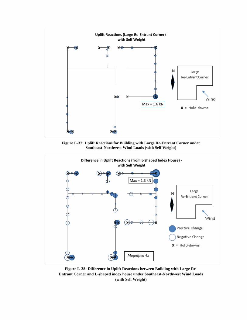
Figure L-37: Uplift Reactions for Building with Large Re-Entrant Corner under
Southeast-Northwest Wind Loads (with Self Weight)
Figure L-38: Difference in Uplift Reactions between Building with Large Re-
Entrant Corner and L-shaped index house under Southeast-Northwest Wind Loads (with Self Weight)
Max = 1.6 kN
Uplift Reactions (Large Re-Entrant Corner) -with Self Weight
N
Max = 1.3 kN
Difference in Uplift Reactions (from L-Shaped Index House) -with Self Weight
N
Magnified 4x

Figure L-39: Lateral Load Distribution to East-West walls under Southeast-
Northwest Wind Loads (with Self Weight)
Figure L-40: Lateral Load Distribution to North-South walls under Southeast-
Northwest Wind Loads (with Self Weight)
0
1
2
3
4
5
6
7
8
9
10
Wall 1 Wall 2 Wall 3 Wall 4
Reac
tion
(kN
)
Lateral Load Distribution to E-W Walls
Small Re-entrant CornerL-Shaped Index HouseMedium Re-entrant CornerLarge Re-entrant Corner
N
0
1
2
3
4
5
6
7
8
9
10
Wall 9 Wall 6,7,8 Wall 5
Reac
tion
(kN
)
Lateral Load Distribution to N-S Walls
Small Re-entrant CornerL-Shaped Index HouseMedium Re-entrant CornerLarge Re-entrant Corner
N

Figure L-41: Unit Shear in North-South walls under Southeast-Northwest Wind Loads (with Self Weight)
0
0.1
0.2
0.3
0.4
0.5
0.6
0.7
0.8
0.9
1
Wall 9 Wall 6,7,8 Wall 5
Uni
t Sue
ar (k
N/m
)
Unit Shear in N-S Walls
Small Re-entrant CornerL-Shaped Index HouseMedium Re-entrant CornerLarge Re-entrant Corner
N