kar.kent.ac.uk 241 The Dual, Localized or Band-Like, Character of the 4f-States W.M. Temmerman, L. Petit†, A. Svane†, Z. Szotek, M. Lu¨ders*, P. …

Kent Academic RepositoryFull text document (pdf)

Copyright & reuse

Content in the Kent Academic Repository is made available for research purposes. Unless otherwise stated all

content is protected by copyright and in the absence of an open licence (eg Creative Commons), permissions

for further reuse of content should be sought from the publisher, author or other copyright holder.

Versions of research

The version in the Kent Academic Repository may differ from the final published version.

Users are advised to check http://kar.kent.ac.uk for the status of the paper. Users should always cite the

published version of record.

Enquiries

For any further enquiries regarding the licence status of this document, please contact:

[email protected]

If you believe this document infringes copyright then please contact the KAR admin team with the take-down

information provided at http://kar.kent.ac.uk/contact.html

Citation for published version

Temmerman, Walter and Petit, Leon and Svane, Axel and Szotek, Zdzislawa and Lueders, M.and Strange, Paul and Staunton, Julie and Hughes, I. D. and Gyorffy, Balazs L. (2009) The Dual,Localized or Band-like Character of the 4f States. In: Gschneider, K. A. and Bunzil, J.-C. G.and Pecharsky, V. K., eds. Handbook on the Physics and Chemistry of Rare Earths. Elsevier,

DOI

https://doi.org/10.1016/S0168-1273(08)00001-9

Link to record in KAR

http://kar.kent.ac.uk/50376/

Document Version

Publisher pdf

Provided for non-commercial research and educational use only.

Not for reproduction, distribution or commercial use.

This chapter was originally published in the book Handbook on the Physics and

Chemistry of Rare Earths, Vol 39, published by Elsevier, and the attached copy is

provided by Elsevier for the author's benefit and for the benefit of the author's

institution, for non-commercial research and educational use including without

limitation use in instruction at your institution, sending it to specific colleagues who

know you, and providing a copy to your institution�s administrator.

All other uses, reproduction and distribution, including without limitation commercial

reprints, selling or licensing copies or access, or posting on open internet sites, your

personal or institution�s website or repository, are prohibited. For exceptions,

permission may be sought for such use through Elsevier's permissions site at:

http://www.elsevier.com/locate/permissionusematerial

From: W.M. Temmerman, L. Petit, A. Svane, Z. Szotek, M. Lüders, P. Strange,

J.B. Staunton, I.D. Hughes, and B.L. Gyorffy, The Dual, Localized or Band-Like,

Character of the 4f-States. In K.A. Gschneidner, Jr., J.-C.G. Bünzli and

V.K. Pecharsky, editors: Handbook on the Physics and Chemistry of Rare Earths,

Vol. 39, Netherlands: North-Holland, 2009, pp. 1-112.

ISBN: 978-0-444-53221-3

© Copyright 2009 Elsevier B.V.

North-Holland

CHAPTER 241

The Dual, Localized or Band-Like,Character of the 4f-States

W.M. Temmerman*, L. Petit†, A. Svane†, Z. Szotek*,

M. Luders*, P. Strange‡, J.B. Staunton}, I.D. Hughes}, and

B.L. Gyorffy}

Contents List of Symbols and Acronyms 2

1. Introduction 4

2. Salient Physical Properties 6

2.1 Lattice parameters 6

2.2 Magnetic properties and magnetic order 8

2.3 Fermi surfaces 12

3. Band Structure Methods 15

3.1 Local spin density approximation 15

3.2 ‘f Core’ approach 18

3.3 OP scheme 18

3.4 Local density approximation þ Hubbard U 19

3.5 Self-interaction-corrected local spin density

approximation 20

3.6 Local self-interaction-corrected local spin density

approximation 24

3.7 The GW method 26

3.8 Dynamical mean field theory 28

4. Valence and Valence Transitions 29

4.1 Determining valence 29

4.2 Valence of elemental lanthanides 30

4.3 Valence of pnictides and chalcogenides 32

4.4 Valence of ytterbium compounds 41

4.5 Valence transitions 43

4.6 Valence of lanthanide oxides 49

Handbook on the Physics and Chemistry of Rare Earths, Volume 39 # 2009 Elsevier B.V.ISSN 0168-1273, DOI: 10.1016/S0168-1273(08)00001-9 All rights reserved.

* Daresbury Laboratory, Daresbury, Warrington WA4 4AD, United Kingdom{ Department of Physics and Astronomy, University of Aarhus, DK-8000 Aarhus C, Denmark{ School of Physical Sciences, University of Kent, Canterbury, Kent, CT2 7NH, United Kingdom} Department of Physics, University of Warwick, Gibbet Hill Road, Coventry, CV4 7AL, United Kingdom} H.H. Wills Physics Laboratory, University of Bristol, Bristol BS8 1TL, United Kingdom

1

Author's personal copy

5. Local Spin and Orbital Magnetic Moments 56

5.1 Hund’s rules 57

5.2 The heavy lanthanides 57

5.3 The light lanthanides 62

6. Spectroscopy 63

6.1 Hubbard-I approach to lanthanide photoemission spectra 64

6.2 Relativistic theory of resonant X-ray scattering 70

7. Finite Temperature Phase Diagrams 75

7.1 Thermal fluctuations 75

7.2 Spin fluctuations: DLM picture 77

7.3 Valence fluctuations 97

8. Dynamical Fluctuations: The ‘Alloy Analogy’ and the Landau

Theory of Phase Transitions 102

9. Conclusions 105

References 105

List of Symbols and Acronyms

a lattice parametera0 Bohr radiusAnk(o), AB (k, E) Bloch spectral function, n is band index and k is the

wave vectorB magnetic fielde electron chargeE (total) energygJ Lande g-factorfql,q´l´ (o) scattering amplitudeFl Slater integralsG Green’s functionGW approximation for the self-energy based on the product of

the Green’s function (G) and the screened Coulombinteraction (W )

h Planck’s constantkB Boltzmann constantL angular momentum operatorl angular momentum quantum numberm electron massn, n(r) electron densityp pressureR rare earthS spin operatorS Wigner Seitz (atomic sphere) radiusSx entropy, where x denotes the specific entropy contributionS(2) direct correlation function of local momentsT temperatureU (Hubbard U), on-site Coulomb interactionU[n] Hartree (classical electrostatic) energy functional

2 W.M. Temmerman et al.


V volumeV(r) potentialxc exchange and correlationZ atomic numberb inverse temperature 1/(kBT)w(q) magnetic susceptibilitymB Bohr magnetonl Spin-orbit coupling parameterO (generalised) grand potentialC(r1, r2, . . .) electronic many body wave functionC(r) Electronic single particle wave functionS self-energyo frequencyASA atomic sphere approximationBSF Bloch spectral functionBZ Brillouin zoneCPA coherent potential approximationDCA dynamical cluster approximationdhcp double hexagonal closed packedDFT density functional theoryDLM disordered local momentDMFT dynamical mean-field theoryDOS density of statesESRF European Synchrotron Radiation Facilityfcc face centered cubicGGA generalized gradient approximationhcp hexagonal closed packedKKR Korringa, Kohn, and RostokerLDA local density approximationLMTO linear muffin-tin orbitalsLSDA local spin density approximationLS spin-orbitLSD local spin densityLSIC local self-interaction correctionMXRS magnetic X-Ray ScatteringOP orbital polarizationPAW Projector augmented waveRKKY Ruderman-Kittel-Kasuya-YoshidaSCF self-consistent fieldSI self-interactionSIC self-interaction correctionSIC-LSD self-interaction-corrected local spin densitySIC-LSDA self-interaction-corrected local spin density approximationWS Wigner SeitzXMaS X-ray magnetic scattering

The Dual, Localized or Band-Like, Character of the 4f-States 3


1. INTRODUCTION

Ab initio calculations for lanthanide solids were performed from the early days ofband theory (Dimmock and Freeman, 1964). These pioneering calculations estab-lished that physical properties of the lanthanides could be described with thef-states being inert and treated as core states. For example, the crystal structures ofthe early lanthanides could be determined without consideration of the 4f-states(Duthie and Pettifor, 1977). Also the magnetic structures of the late lanthanidescould be evaluated that way (Nordstrom and Mavromaras, 2000). Of course, oneneeded to postulate the number of s, p, and d valence electrons that is three in thecase of a trivalent lanthanide solid or two in the case of a divalent lanthanide solid.Even this valence could be calculated in a semi-phenomenological way withouttaking the 4f-electrons explicitly into account (Delin et al., 1997).

However, in some lanthanides, in particular the Ce compounds, and CeB6

(Langford et al., 1990) is an example, the 4f-level could either be part of the valencestates or be inert and form part of the core. Fermiology measurements coulddetermine how many electrons participated in the Fermi surface and hencecould deduce the nature of the 4f-state as either part of the core or part of thevalence states. These measurements were complemented by band structure cal-culations of the type ‘4f-core’ or ‘4f-band’, respectively treating the 4f-states aspart of the core or as valence states.

Treating the 4f-electrons in Gd as valence states, in the ‘4f-band’ approach,allowed for an accurate description of the Fermi surface (Temmerman and Sterne,1990) but failed in obtaining the correct magnetic structure (Heinemann andTemmerman, 1994). What these and numerous other calculations demonstratedwas that some properties of the lanthanides could be explained by a ‘4f-band’framework and some by a ‘4f-core’ framework. This obviously implied a dualcharacter of the 4f electron in lanthanides: some of the 4f-electrons are inert andare part of the core, some of the 4f-electrons are part of the valence and contributeto the Fermi surface.

The correct treatment of the 4f electrons in lanthanides is a great challenge ofany modern theory. On the one hand, when considering the spatial extent of theiratomic orbitals, the 4f electrons are confined to the region close to the nuclei, thatis, they are very core-like. On the other hand, with respect to their position inenergy, which is often in the vicinity of the Fermi level, they should rather beclassified as valence electrons. Some of the most widely used theoretical methodsfor the description of lanthanide systems are based on DFT (Hohenberg and Kohn,1964). Its basic concept is the energy functional of the total charge density of theelectrons in the solid that, when minimized for given nuclear positions, providesthe energy as well as the charge density of the ground state. However, for solids,the exact DFT energy functional is not known, and one is forced to use approx-imations, of which the most successful is the LSDA, where electron correlationsare treated at the level of the homogeneous electron gas, and the f electrons aredescribed by extended Bloch states, as all the other, s, p, and d, electrons are. Buteven in this approach, one can try to differentiate between the f and otherelectrons, by including them into the core (‘f-core’ approach). One step beyond



the local approximation, there are various flavours of the so-called GGAs, which,in addition to the dependence on a homogeneous charge distribution, include alsosome gradient corrections. Unfortunately, neither LDA nor GGA have provedvery successful for systems where f electrons have a truly localized nature. Here,the SIC-LSD approaches have shown to be most useful, in particular as far as thecohesive properties are concerned.

The SIC-LSDA (Perdew and Zunger, 1981) provides an ab initio computationalscheme that allows the differentiation between band-like and core-like f-electron(Temmerman et al., 1998). This is a consequence of the SIC being only substantialfor localized states, which the 4f-states are. From this, one would expect to applythe SIC to all 4f-states since the delocalized s, p, and d electrons are not experien-cing any self-interaction. But we do not know how many localized 4f-states thereare. For a divalent lanthanide, there is one more localized 4f electron than for atrivalent lanthanide. To determine how many localized 4f electrons there are in aparticular 4f-solid, we can be guided byminimizing the SIC-LSD total energy overall possible configurations of localized (SIC) and itinerant 4f-states. This chapterelaborates on the consequences of this, naturally leading to the dual character ofthe 4f electron: either localized after applying the SIC or LSD band-like andcontributing to the Fermi surface. The SIC-LSD method forms the basis of mostof the work reviewed in this chapter, and its focus will be on the total energyaspect and, as we will show, provides a quite accurate description of the cohesiveproperties throughout the lanthanide series.

Other known methods that have been used in the study of lanthanides includethe OP scheme, the LDAþU approach, whereU is the on-site Hubbard repulsion,and the DMFT, being the most recent and also the most advanced development. Inparticular, when combined with LDA þ U, the so-called LDA þ DMFT scheme, ithas been rather successful for many complex systems. We note here that bothDMFT and LDA þ U focus mostly on spectroscopies and excited states (quasi-particles), expressed via the spectral DOS. In a recent review article (Held, 2007),the application of the LDA þ DMFT to volume collapse in Ce was discussed.Finally, the GW approximation and method, based on an electron self-energyobtained by calculating the lowest order diagram in the dynamically screenedCoulomb interaction, aims mainly at an improved description of excitations, andits most successful applications have been for weakly correlated systems. How-ever, recently, there have been applications of the quasi-particle self-consistentGW method to localized 4f systems (Chantis et al., 2007).

The outline of the present chapter is as follows. Section 2 deals with the relevantphysical, electronic, and magnetic properties of the lanthanides. Section 3 reviewsbriefly the above-mentioned theoretical methods, with the focus on the SIC-LSDAmethod, and, in particular, the full implementation of SIC, involving repeatedtransformations between Bloch and Wannier representations (Temmerman et al.,1998). This is then compared with the local-SIC, implemented in the multiplescattering theory (Luders et al., 2005). Section 4 deals with the valence (Strangeet al., 1999) and valence transitions of the lanthanides. Section 5 discusses the localmagnetic moments of the lanthanides. Section 6 discusses two spectroscopiesapplied to lanthanides and some of their compounds. Section 7 outlines a method-ology of calculating the finite temperature (T) properties of the lanthanides and their



compounds, and illustrates it on the study of finite T magnetism of the heavylanthanides and the finite T diagram of the Ce a–g phase transition. The ab initiotheory of the finite T magnetism is based on the calculations of the paramagneticsusceptibilitywithin theDLMpicture (Gyorffy et al., 1985). This combinedDLMandSIC approach (Hughes et al., 2007) for localized states provides an ab initio descrip-tion of the magnetic properties of ionic systems, without the need of mapping ontothe Heisenberg Hamiltonian. Finally, Section 8 addresses some remaining issuessuch as how to include dynamical fluctuations, and Section 9 concludes this chapter.

2. SALIENT PHYSICAL PROPERTIES

Thephysical properties of the lanthanides are ratherunique amongallmetals. This isthe consequence of the interaction of delocalized conduction electrons with thelocalized f-states. The physical properties are characterized by the continuouslydecreasing lattice parameter upon traversing the lanthanide series, the so-calledlanthanide contraction. Their physical properties can be described very efficiently,and also catalogued, by the valence of the lanthanide. Most of the lanthanides andtheir compounds are trivalent, but towards themiddle and the end of the lanthanideseries, divalence (Sm, Eu, Tm, Yb) can occur. At the very beginning of the lanthanideseries, in Ce and Pr and their compounds, also tetravalence is sometimes observed.For tetravalent Ce and Pr and their compounds, strong quasi-particle renormaliza-tion occurs and some Ce compounds exhibit heavy fermion behaviour. For lantha-nides with higher atomic number than Pr, trivalence establishes itself, however,switching to divalence in Eu and some of the Sm and Eu compounds. For Gd, thef-shell is half-filled and the valence starts again, as in the beginning of the lanthanideseries, as strongly trivalent andgradually reducing todivalenceas seen inYbandTmcompounds. Fingerprints of the valencies can be seen in the value of the spin andorbital magnetic moments and of the lattice parameter: divalent lattice parameterscan be 10% larger than trivalent ones. Also the nature of the multiplet structure tellsus about the valence, as do Fermiologymeasurements, by providing information onthe number of f-states contributing to the Fermi surface. Finally, MXRS hasthe potential to determine the valence as well as to provide information on thesymmetry of the localized states (Arola et al., 2004).

2.1 Lattice parameters

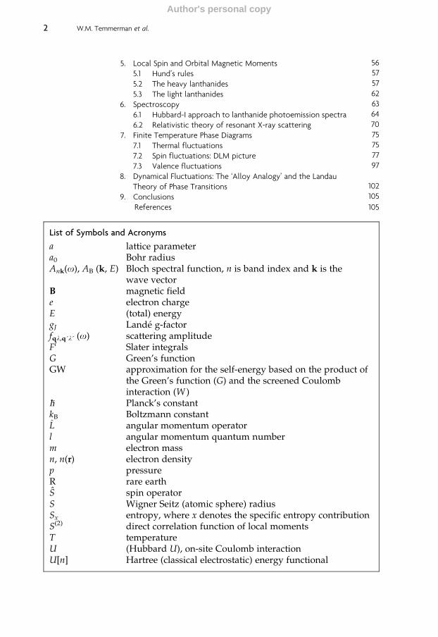
Theexperimental latticeparameters as a functionof lanthanide atomicnumber showthe famous lanthanide contraction, the decrease of the lattice parameter across thelanthanide series, with the exception of the two anomalies for Eu and Yb, as seen inFigure 1 (top panel). What is plotted there is actually the atomic sphere radius S (inatomic units) as a function of the lanthanide element. A similar behaviour is alsoobserved, for example, for lanthanide monochalcogenides and monopnictides,whose lattice parameters are also shown in Figure 1 (middle and bottom panels).

This lanthanide contraction is associated with the filling of the 4f shell across thelanthanide series. The effect is mainly due to an incomplete shielding of the nuclearcharge by the 4f electrons and yields a contraction of the radii of outer electron shells.



5.4

4.6

5.0

5.5

6.0

6.5

5.7

6.0

6.3

6.6

a (

Å)

a (

Å)

6.9

1.8

2.0

2.2

A

B

CLa

La

RSRSeRTe

RAsRPRN

La

S (

Å)

Pr Nd PmSm Eu Gd Tb Dy Ho Er Tm Yb

Ce

Ce

Pr Nd PmSm Eu Gd Tb Dy Ho Er Tm Yb Lu

Ce Pr Nd PmSm Eu Gd Tb Dy Ho Er Tm Yb

FIGURE 1 Lattice constants of the elemental lanthanides (top), their chalcogenides (middle)

(after Jayaraman, 1979), and pnictides (bottom). For the elemental lanthanides, it is the atomic

sphere radius, S, that is shown instead of the lattice parameter, where S is defined as V ¼ 4=3pS3

with V the unit cell volume.



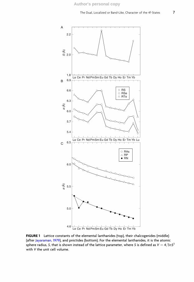
The jumps in the lattice constants in Figure 1, seen for the elemental Eu and Yb,as well as at the chalcogenides of Sm, Eu, Tm, and Yb, are due to the change invalence from trivalent to divalent. If a transition to the trivalent state were tooccur, the lattice constant would also follow the monotonous behaviour of theother lanthanides, as seen in Figure 2, where the ionic radii of trivalent lanthanideions are displayed. For the pnictides, only CeN shows an anomaly, indicating atetravalent state, whereas all the other compounds show a smooth, decreasingbehaviour as a function of the lanthanide atomic number.

Pressure studies have been able to unravel a lot of the physics of the rareearths. Not only have pressure experiments seen changes of valence from divalentto trivalent, but also changes in the structural properties. In the case of Ce and Cecompounds, the valence changes under pressure from trivalent to tetravalent orfrom one localized f-state to a delocalized state have been observed. This will bediscussed in greater detail in Section 4 of this chapter.

2.2 Magnetic properties and magnetic order

The lanthanides are characterized by local magnetic moments coming from theirhighly localized 4f electron states. These moments polarize the conduction elec-trons which then mediate the long range magnetic interaction among them. TheRKKY interaction is the simplest example of this mechanism. These long rangemagnetic interactions in lanthanide solids lead to the formation of a wide varietyof magnetic structures, the periodicities of which are often incommensurate withthe underlying crystal lattice. These are helical structures that have been studiedin detail with neutron scattering (Sinha, 1978; Jensen andMackintosh, 1991). In thelater sections of this chapter, we shall elaborate on our ab initio study of the finitetemperature magnetism of the heavy lanthanides and elucidate the role of theconduction electrons in establishing the complex helical structures in these sys-tems. This ab initio theory and calculations go beyond the ‘standard model’ oflanthanide magnetism ( Jensen and Mackintosh, 1991).

The standard approach to describing the magnetism of lanthanides, and inparticular their magnetic moments, is to assume the picture of electrons in an

CeLa0.85

0.90

0.95

1.00

1.05

R3+

(Å

)

LuYbTmErHoDyTbGdEuSmPmNdPr

FIGURE 2 Ionic radii of trivalent lanthanides.



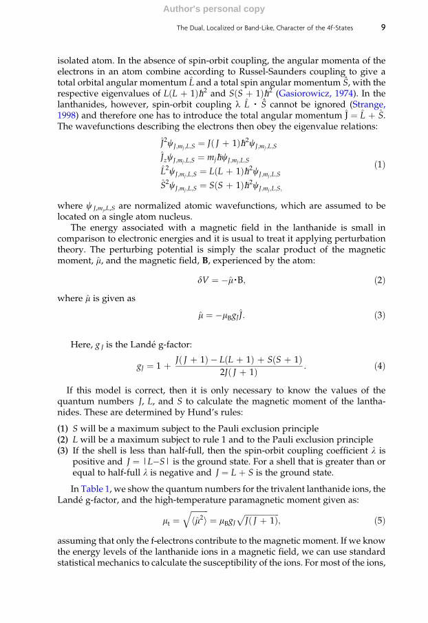
isolated atom. In the absence of spin-orbit coupling, the angular momenta of theelectrons in an atom combine according to Russel-Saunders coupling to give atotal orbital angular momentum L and a total spin angular momentum S, with therespective eigenvalues of L L þ 1ð Þh2 and S S þ 1ð Þh2 (Gasiorowicz, 1974). In thelanthanides, however, spin-orbit coupling l L � S cannot be ignored (Strange,1998) and therefore one has to introduce the total angular momentum J ¼ L þ S.The wavefunctions describing the electrons then obey the eigenvalue relations:

J2cJ;mj;L;S¼ J J þ 1ð Þh2cJ;mj;L;S

JzcJ;mj;L;S¼ mjhcJ;mj;L;S

L2cJ;mj;L;S¼ L L þ 1ð Þh2cJ;mj;L;S

S2cJ;mj;L;S¼ S S þ 1ð Þh2cJ;mj;L;S;

ð1Þ

where c J,mj,L,S are normalized atomic wavefunctions, which are assumed to belocated on a single atom nucleus.

The energy associated with a magnetic field in the lanthanide is small incomparison to electronic energies and it is usual to treat it applying perturbationtheory. The perturbing potential is simply the scalar product of the magneticmoment, m, and the magnetic field, B, experienced by the atom:

dV ¼ �m�B; ð2Þ

where m is given as

m ¼ �mBgJ J: ð3Þ

Here, g J is the Lande g-factor:

gJ ¼ 1 þ J J þ 1ð Þ � L L þ 1ð Þ þ S S þ 1ð Þ2J J þ 1ð Þ : ð4Þ

If this model is correct, then it is only necessary to know the values of thequantum numbers J, L, and S to calculate the magnetic moment of the lantha-nides. These are determined by Hund’s rules:

(1) S will be a maximum subject to the Pauli exclusion principle(2) L will be a maximum subject to rule 1 and to the Pauli exclusion principle(3) If the shell is less than half-full, then the spin-orbit coupling coefficient l is

positive and J ¼ |L�S| is the ground state. For a shell that is greater than orequal to half-full l is negative and J ¼ L þ S is the ground state.

In Table 1, we show the quantum numbers for the trivalent lanthanide ions, theLande g-factor, and the high-temperature paramagnetic moment given as:

mt ¼ffiffiffiffiffiffiffiffiffi

hm2iq

¼ mBgJffiffiffiffiffiffiffiffiffiffiffiffiffiffiffiffiffiffi

J J þ 1ð Þp

; ð5Þ

assuming that only the f-electrons contribute to the magnetic moment. If we knowthe energy levels of the lanthanide ions in a magnetic field, we can use standardstatistical mechanics to calculate the susceptibility of the ions. For most of the ions,



the difference in energy between the first excited state and the ground state ismuch greater than kBT at room temperature, where kB is the Boltzmann constant,and essentially only the ground state is populated. This enables us to derive theCurie formula

w ¼ Nhm2i3kBT

ð6Þ

for the susceptibility of a system of N non-interacting ions. More realistically, thisformula should be replaced by the Curie-Weiss law, where the T in the denomi-nator in Eq. (6) is replaced by T�Tc, where Tc is the magnetic ordering tempera-ture. The Curie-Weiss formula was employed to determine the experimentalmagnetic moments, me, in Table 1. For Sm3þ and Eu2þ, the first excitedlevel is within kBT of the ground state and so is appreciably populated. To describethese two ions with numerical accuracy, it is necessary to sum over the allowedvalues of J and recall that each J contains 2J þ 1 states. The susceptibilitythen becomes considerably more complicated but does give a good descriptionof Sm3þ and Eu2þ.

The theoretical magnetic moments in Table 1 are for single trivalent ionsassuming no inter-ionic interactions. However, the experiments are performedon metallic elements where each individual ion is embedded in a crystal and feels

TABLE 1 Quantum numbers and total f-electron magnetic moments of the trivalent lanthanide

ions. mt is the magnetic moment calculated from Eq. (5). me is the measured magnetic moment.

All magnetic moments are expressed in Bohr magnetons

S L J Ground state gj mt mea

La 0.00 0.00 0.00 1S0Ce 0.50 3.00 2.50 2F5/2 6/7 2.54 2.4Pr 1.00 5.00 4.00 3H4 4/5 3.58 3.5Nd 1.50 6.00 4.50 4I9/2 8/11 3.62 3.5Pm 2.00 6.00 4.00 5I4 3/5 2.68Sm 2.50 5.00 2.50 6H5/2 2/7 0.85 1.5b

Eu 3.00 3.00 0.00 7F0 0.0 3.4b,c

Gd 3.50 0.00 3.50 8S7/2 2 7.94 7.95Tb 3.00 3.00 6.00 7F6 3/2 9.72 9.5Dy 2.50 5.00 7.50 6H15/2 4/3 10.65 10.6Ho 2.00 6.00 8.00 5I8 5/4 10.61 10.4Er 1.50 6.00 7.50 4I15/2 6/5 9.58 9.5Tm 1.00 5.00 6.00 3H6 7/6 7.56 7.3Yb 0.50 3.00 3.50 2F7/2 8/7 4.54 4.5Lu 0.00 0.00 0.00 1S0

a All experimental values taken from Kittel (1986).b See text.c Eu usually exists in the divalent form.



the crystalline electric field, which arises from charges on neighbouring ions. Theexcellent agreement between the magnetic moment measured experimentally andthat obtained from Eq. (5) implies that the 4f-electrons are so well shielded that theeffect of the crystalline environment can be neglected and the agreement withEq. (6) supports this view. With the agreement between theory and experimentdisplayed in Table 1, it might reasonably be assumed that the magnetic momentsof the lanthanide metals are well understood. While this is probably true qualita-tively, it is certainly not true quantitatively. Questions about this model that maybe raised are:

(1) In the solid state, the interactionwith the sea of conduction electrons distorts thepure atomic picture, and multiplets other than the Hund’s rule ground statemix into the full wave function. In view of the success of the atomic approxima-tion, it is likely that this mixing of different J quantum numbers is at the fewpercent level, nonetheless this is an assumption that should be tested.

(2) The eigenfunctions CJ,mj,L,S in Eq. (1) are generally quantum mechanicallyentangled, given as sums of Slater determinants constructed from atomicsingle-electron orbitals. The description of entangled quantum states in asolid state environment is extremely difficult. With the recent introductionof the DMFT (Section 3.8), one might have developed a scheme for this,however, more investigations are needed. Usually, one resorts to the indepen-dent particle approximation thus ignoring the ‘many-body’ nature of thewavefunction and the localized f-manifold is represented by a single ‘bestchoice’ Slater determinant. This is the approach taken in the various DFTschemes, including the SIC-LSD theory to be described in Section 3.5. Howcould such a picture arise from a more sophisticated and realistic descriptionof the electronic structure of the lanthanides?

(3) The picture of lanthanide magnetism described above is for independenttrivalent lanthanide ions. Thus, it does not explain cooperative magnetism,that is ordered magnetic structures which are the most common low-temperature ground states of lanthanide solids. Our view of a lanthanidecrystal is of a regular array of such ions in a sea of conduction electrons towhich each ion has donated three electrons. For cooperative magnetism toexist, those ions must communicate with one another somehow. It is generallyaccepted that this occurs through indirect exchange in the lanthanide metals,the simplest example of this being the RKKY interaction (Ruderman andKittel, 1954; Kasuya, 1956; Yosida, 1957). However, for this to occur, theconduction sd-electrons themselves must be polarized. This conduction elec-tron polarization has been calculated using DFTmany times and is found to besubstantial. There have been many successes in descriptions of magneticstructures, some of which will be discussed in Section 7.2. However, interms of the size of magnetic moments, the agreement between theory andexperiment shown in Table 1 is considerably worsened (see discussion inSection 5). Why is this?



(4) If the atomic model were rigorously correct, a lanthanide element would havethe same magnetic moment in every material and crystalline environment. Ofcourse, this is not the case, and more advanced methods have to be employedto determine the effect of the crystalline and chemical environment on mag-netic moments with numerical precision. Examples of materials where thetheory described above fails to give an accurate value for the lanthanide ionmagnetic moment are ubiquitous. They include NdCo5 (Alameda et al., 1982),fullerene encapsulated lanthanide ions (Mirone, 2005), and lanthanide pyro-chlores (Hassan et al., 2003).

In conclusion, it is clear that the standard model makes an excellent firstapproximation to the magnetic properties of lanthanide materials, but to under-stand lanthanide materials on a detailed individual basis, a more sophisticatedapproach is required.

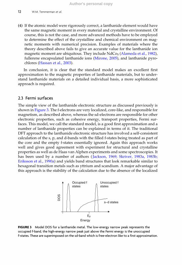
2.3 Fermi surfaces

The simple view of the lanthanide electronic structure as discussed previously isshown in Figure 3. The f-electrons are very localized, core-like, and responsible formagnetism, as described above, whereas the sd-electrons are responsible for otherelectronic properties, such as cohesive energy, transport properties, Fermi sur-faces. This model, we call the standard model, is a good first approximation and anumber of lanthanide properties can be explained in terms of it. The traditionalDFT approach to the lanthanide electronic structure has involved a self-consistentcalculation of the s, p, and d-bands with the filled f-states being treated as part ofthe core and the empty f-states essentially ignored. Again this approach workswell and gives good agreement with experiment for structural and crystallineproperties as well as de Haas van Alphen experiments and some spectroscopies. Ithas been used by a number of authors ( Jackson, 1969; Skriver, 1983a, 1983b;Eriksson et al., 1990a) and yields band structures that look remarkable similar tohexagonal transition metals such as yttrium and scandium. A major advantage ofthis approach is the stability of the calculation due to the absence of the localized

Unoccupied fstates

EF

Energy

s−d states

Occupied fstates

DO

S

FIGURE 3 Model DOS for a lanthanide metal. The low-energy narrow peak represents the

occupied f-band, the high-energy narrow peak just above the Fermi energy is the unoccupied

f-states. These are superimposed on the sd-band which is free-electron like to a first approximation.



4fs. Both Skriver (1983b) and Eriksson et al. (1990a) have performed a successfulcalculation of the cohesive properties and the work of Skriver reproduces well thecrystal structures which are sensitively dependent on the details of the valenceband. For example, the partial 5d occupation numbers decrease across the serieswith a corresponding increase in the 6s occupation. The increase in 5d occupationis what causes the structural sequence hcp ! Sm structure ! dhcp ! fcc as theatomic number decreases or the pressure increases (Duthie and Pettifor, 1977). Adetailed analysis of Jackson’s work ( Jackson, 1969) on Tb yields a Fermi surfacethat shows features with wave vector separations corresponding to the character-istic wave vector describing the spiral phase of Tb.

One of the successes of this approach is the comparison of calculated electronicstructures with de Haas van Alphen measurements. The investigations of theFermi surface of Gd using this technique among others were pioneeredby Young and co-workers (Young et al., 1973; Mattocks and Young, 1977) andextended by Schirber and co-workers (Schirber et al., 1976). These studies foundfour frequencies along the c-direction and three in the basal plane and later workfound a number of small frequencies (Sondhelm and Young, 1977). All thesefrequencies could be accounted for on the basis of the band structure calculationsof the time. Sondhelm and Young also measured cyclotron masses and massenhancements in Gd and found values in the region of 1.2–2.1 which were inagreement with the band structure calculations, but were rather smaller thanthose derived from low-temperature heat capacity measurements. More recently,angle-resolved photoemission have been used for Fermi surface studies of Tb(Dobrich et al., 2007) and also Dy and Ho metals were studied (Schußler-Langeheine et al., 2000). Fermi surfaces of Gd-Y alloys were studied with positronannihilation (Fretwell et al., 1999; Crowe et al., 2004). In particular, the changes tothe Fermi surface topology upon the transition from ferromagnetism to helicalanti-ferromagnetism could be followed. Concerning the light lanthanides, theFermi surface areas and cyclotron masses in Pr were measured (Wulff et al.,1988) with the de Haas van Alphen technique. Large mass enhancements, espe-cially for an elemental metal, were measured and the understanding of the Fermisurface needed an approach well beyond the standard model (Temmerman et al.,1993).

This standard model does have several major drawbacks:

(1) It can never get the magnetic properties correct.(2) It cannot describe systems with large mass enhancements.(3) There is one overarching shortcoming of the standard model, which is slightly

more philosophical. It treats the f-electrons as localized and the sd-electrons asitinerant, that is, it treats electrons within the same material on a completelydifferent basis. This is aesthetically unsatisfactory and furthermore makes itimpossible to define a reference energy. In principle, one has to know, a priori,which electrons to treat as band electrons and which to treat as core electrons.It would be infinitely better if the theory itself contained the possibility of bothlocalized and itinerant behaviour and it chose for itself how to describe theelectrons.



For two elements, it is possible to perform LDA calculations including thef-electrons in the self-consistency cycle. The first is cerium where the f-electronsare not necessarily localized. Cerium and its compounds are right on the borderbetween localized and itinerant behaviour of the 4f electrons. There has beenmuch controversy over the nature of the f-state in materials containing cerium.The key issue is the g–a phase transition where the localized magnetic momentassociated with a 4f1 configuration disappears with an associated volume collapseof around 14–17%, but no change in crystal symmetry. The f electron count isthought to be around one in both phases of Ce. What appears to be happeninghere is a transition from a localized to a delocalized f-state (Pickett et al., 1981;Fujimori, 1983). Both Pickett et al. (1981) and Fujimori (1983) highlight the limita-tions of the band theory picture for cerium. In particular, Fujimori discusses thecalculation of photoemission spectra and the reasons why band theory does notdescribe such spectroscopies well. The a-phase can be described satisfactorilyusing the standard band theory, while there is more difficulty in describing theg-phase and the energy difference between the two phases (which is very small onthe electronic scale) is not calculated correctly. The second lanthanide elementwhere band theory may hope to shed some light on its properties is gadolinium.Here the f-levels are spilt into seven filled majority spin and seven unfilledminority spin bands, neither of which are close to the Fermi energy. It is feasibleto perform a DFT calculation and converge to a reasonable result. This has beendone by a number of authors ( Jackson, 1969; Ahuja et al., 1994; Temmerman andSterne, 1990) with mixed results. Temmerman and Sterne were among the first toindicate that the semi-band nature of the 5p levels could significantly influencepredicted properties. Sandratsakii and Kubler (1993) took this work a bit furtherby investigating the stability of the conduction band moment with respect todisorder in the localized 4f-moment.

The experimentally determined Fermi surface of Gd (Schirber et al., 1976;Mattocks and Young, 1977) has been used by several band structure calculationsto determine whether the f-states have to be treated as core-like or band-like. Gdmetal is the most thoroughly studied of all the lanthanides and one of the fewlanthanides that have been studied by the de Haas van Alphen technique(Schirber et al., 1976; Mattocks and Young, 1977). Being trivalent, it has, throughthe exchange splitting, a half-filled f-shell. The Gd f-states are well separated fromthe Fermi level, and therefore f-states are not contributing to the Fermi surface. Thiswas seen in the Fermiology measurements (Schirber et al., 1976; Mattocks andYoung, 1977). Both f-core (Richter and Eschrig, 1989; Ahuja et al., 1994) and f-band(Sticht and Kubler, 1985; Krutzen and Springelkamp, 1989; Temmerman and Sterne,1990; Singh, 1991) calculations claim to be able to describe this Fermi surface.

While these methods provide some useful insight into Gd and Ce, they yieldunrealistic results for any other lanthanide material as the f-bands bunch at theFermi level leading to unphysically large densities of states at the Fermi energyand disagreement with the de Haas van Alphen measurements. It is clear that asatisfactory theory of lanthanide electronic structures requires a method thattreats all electrons on an equal footing and fromwhich both localized and itinerantbehaviour of electrons may be derived. SIC to the LSDA provide one such theory.



This method is based on DFT and the free electron liquid, but corrects it forelectrons where self-interactions are significant and takes the theory towards amore localized description.

3. BAND STRUCTURE METHODS

As described in Section 1, there exist many theoretical approaches to calculatingelectronic structure of solids, and most of them have also been applied to lantha-nides. In this section, we shall briefly overview some of the most widely used,focusing however on the SIC-LSD, in both full and local implementations, as thisis the method of choice for most of the calculations reported in this chapter. Thesimplest approach to deal with the f electrons is to treat them like any otherelectron, that is, as itinerant band states. Hence, we start our review of modernmethods with a brief account of the standard LDA and its spin-polarized version,namely the LSD approximation. We also comment on the use of LSD in the cases,where one restricts the variational space by fixing the assumed number off electrons to be in the (chemically inert) core (‘f-core’ approach). Following this,we then briefly overview the basics of other, more advanced, electronic structuremethods mentioned in Section 1, as opposed to a more elaborate description of theSIC-LSD method.

3.1 Local spin density approximation

DFT relies on the proof (Hohenberg and Kohn, 1964; Kohn and Sham, 1965;Dreizler and Gross, 1990; Martin, 2004) that for any non-degenerate many-electron system, there exists an energy functional E[n], where n(r) is the electroncharge density in space-point r, which when minimized (with respect to n(r))provides the correct ground state energy as well as ground state electron chargedensity. Hence, the charge density n(r), rather than the full many-electron wave-function C(r1, r2, . . ., rN), becomes the basic variable, which constitutes a simplifi-cation from a complex-valued function depending on N sets of space coordinatesto a non-negative function of only one set of space coordinates. The price paid isthat the exact functional form of E[n] is unknown, and presumably of suchcomplexity that it will never be known. However, approximations of high accu-racy for a diversity of applications exist and allow predictive investigations ofmany novel functional materials in condensed matter physics and materialsscience. The great advance in the field was facilitated by the observation (Kohnand Sham, 1965) that if one separates out from the total energy functional, E[n], thekinetic energy, T0[n], of a non-interacting electron gas with charge density n(r)(which does not coincide with the true kinetic energy of the system), and theclassical electrostatic energy terms, then simple, yet accurate, functionals may befound to approximate the remainder, called the exchange-correlation (xc) energyfunctional Exc[n]. Thus, the total energy functional can be written as

E n½ � ¼ T0 n½ � þ U n½ � þ Vext n½ � þ Exc n½ �; ð7Þ



where the electron–electron interaction (Hartree term) is given by

U n½ � ¼ð ð

n rð Þn r0ð Þr� r0j j d3rd3r0; ð8Þ

and the external potential energy, Vext[n], due to electron–ion and ion–ion inter-actions, respectively, is

Vext n½ � ¼ð

n rð ÞVion rð Þd3r þ Eion;ion: ð9Þ

Here Vion(r) is the potential from the ions, and the atomic Rydberg unitse2=2 ¼ 2m ¼ h ¼ 1� �

have been used in all the formulas. Since Eqs. (8) and (9)are explicitly defined in terms of the electron charge density, all approximationsare applied to the last term in Eq. (7), the exchange and correlation energy.

In the LDA, it is assumed that each point in space contributes additively to Exc:

ELDAxc n½ � ¼

ð

n rð Þehom n rð Þð Þd3r; ð10Þ

where ehom(n) is the exchange and correlation energy of a homogeneous electrongas with charge density n. In the simplest case, when only exchange is considered,one has (Hohenberg and Kohn, 1964)

ehom nð Þ ¼ �Cn1=3 with C ¼ 3

2

3

p

� �1=3

: ð11Þ

Modern functionals include more elaborate expressions for ehom(n) (Voskoet al., 1980; Perdew and Zunger, 1981) relying on accurate Quantum MonteCarlo data for the homogeneous electron gas (Ceperley and Alder, 1980). General-izing to magnetic solids, which is highly relevant for lanthanide materials, isstraightforward as one merely has to consider two densities, one for spin-upand one for spin-down electrons, which corresponds to the LSD functional (vonBarth andHedin, 1972), ELSD. Evenmore accurate calculations may be obtained byincluding corrections for the spatial variation of the electron charge density,which is accomplished by letting ehom also be dependent on gradients of thecharge density, which constitutes the GGA (Perdew and Wang, 1992). Yet moreaccurate functionals may be composed by mixing some non-local exchange inter-action into the Exc (Becke, 1993), often named hybrid functionals.

The minimization of E[n], with these approximate functionals, is accomplishedby solving a one-particle Schrodinger equation for an effective potential, whichincludes an exchange-correlation part given by the functional derivative of Exc[n]with respect to n(r). The non-interacting electron gas system with the chargedensity n(r) is generated by populating the appropriate number of lowest energysolutions (the aufbau principle). Self-consistency must be reached between thecharge density put into the effective potential and the charge density composedfrom the occupied eigenstates. This is usually accomplished by iterating theprocedure until this condition is fulfilled.



Spin-orbit interaction is only included in the density functional framework ifthe proper fully relativistic formalism is invoked (Strange, 1998). Often an approx-imate treatment of relativistic effects is implemented, by solving for the kineticenergy in the scalar-relativistic approximation (Skriver, 1983a), and adding to thetotal energy functional the spin-orbit term as a perturbation of the form

Eso ¼X

occ:

a

hcajxð r!Þ l

!� s! jcai; ð12Þ

where the sum extends over all occupied states caij and x is the spin-orbitparameter. Here l

!and s!denote the one-particle operators for angular and spin

moments. The method presupposes, which usually does not pose problems, thatan appropriate region around each atommay be defined inside which the angularmomentum operator acts.

The LDA and LSD, as well as their gradient corrected improvements, havebeen extremely successful in providing accurate, material specific, electronic,magnetic, and structural properties of a variety of weakly to moderatelycorrelated solids, in terms of their ground state charge density ( Jones andGunnarsson, 1989; Kubler, 2000), However, these approaches often fail for sys-tems containing both itinerant and localized electrons, and in particular d- and f-electron materials. For all lanthanides, and similarly the actinide elements beyondneptunium, the electron correlations are not adequately represented by LDA. Ind-electronmaterials, for example, transitionmetal oxides, this inadequate descrip-tion of localized electrons leads commonly to the prediction of wrong magneticground states and/or too small or non-existent band gaps and magnetic moments.

When applied to lanthanide systems, LSD (and GGA as well) leads to theformation of narrow bands which tend to fix and straddle the Fermi level. Due totheir spatially confined nature, the f-orbitals hybridize only weakly and barely feelthe crystal fields. Furthermore, on occupying the f-band states, the repulsive poten-tial on the lanthanide increases due to the strong f–f Coulomb repulsion, so thef-bands fill up to the point where the total effective potential pins the f-states at theFermi level. Generally, the band scenario leads to distinct overbinding (when com-pared to experimental data), since the occupation of the most advantageous f-bandstates favours crystal contraction (leading to increase in hybridization). Hence, thepartially filled f-bands provide a negative pressure, which in most cases is unphy-sical. The same effect iswell known to cause the characteristic parabolic behaviour ofthe specific volumes of the transition metals, and would lead to a similar parabolicbehaviour for the specific volumes of the lanthanides, which is in variance with theobservation seen in Figure 1 in Section 2.1. This will be discussed further in Section4.2. Even if narrow, the f-bands in the vicinity of the Fermi level alone cannotdescribe the heavy fermion behaviour seen in many cerium and ytterbium com-pounds. Zwicknagl (1992) and co-workers applied a renormalization scheme toLDA band structures to describe the heavy fermion properties with successfulapplication in particular to the understanding of Fermi surfaces.



3.2 ‘f Core’ approach

To remedy the failure of LSD, it was early realized that one could remove thespurious bonding due to f-bands by simply projecting out the f-degrees of freedomfrom variational space and instead include the appropriate number of f electrons inthe core. This approach was used to study the crystal structures of the lanthanideelements (Duthie and Pettifor, 1977; Delin et al., 1998), which are determined by thenumber of occupied d-states. In this approach, the lanthanide contraction neatlyfollows as an effect of the incomplete screening of the increasing nuclear charge byadded f electrons, as one moves through the lanthanide series ( Johansson andRosengren, 1975). In a recent application, the ‘f core’ approach proved useful inthe study of complex magnetic structures (Nordstrom and Mavromaras, 2000).

Johansson and co-workers have extended the ‘f core’ approach to computeenergies of lanthanide solids, with different valencies assumed for the lanthanideion, by combining the calculated LSD total energy for the corresponding ‘f core’configurations with experimental spectroscopic data for the free atom (Delin et al.,1997). This scheme correctly describes the trends in cohesive energies of thelanthanide metals, including the valence jumps at Eu and Yb, as well as theintricate valencies of Sm and Tm compounds.

3.3 OP scheme

The OP scheme was introduced by Eriksson et al. (1990b) to reduce the bonding off-electrons without totally removing them from the active variational space. Theidea copies the way spin polarization leads to reduced bonding if the exchangeparameter is large enough (Kubler and Eyert, 1993). An extra term is added to theLSD functional (7):

EOP n½ � ¼ ELSD n½ � �X

i

E3i L

2zi; ð13Þ

where i numbers the atomic sites, Lzi is the total z-component of the orbitalmoment, and E3

i is a parameter (the Racah parameter), which can be calculatedfrom an appropriate combination of Slater integrals (Eriksson et al., 1990b). Theadded term favours the formation of an orbital moment and adds a potential shift�E3

i Lziml to each f orbital, where ml is the azimuthal quantum number of thef electron considered. The effect is to partially split the f-band into 14 distinctbands (if the E3 parameter exceeds hybridization and crystal fields). Since com-pression enhances the latter two effects, the OP scheme could successfullydescribe the g–a transition of cerium as a transition from large to low orbitalmoment (Eriksson et al., 1990b). This is then to be interpreted as a Mott-typetransition in the f-manifold from a localized to a band-like behaviour. The OPscheme has also been applied to the pressure-induced volume collapse in Pr(Svane et al., 1997). Generally, the OP term is too small in magnitude to fullydescribe the inertness of the f electrons in the lanthanide series beyond Pr. The OPscheme has been most successful in describing the orbital moment contribution to



itinerant systems, for example 3d-transition metal and actinide compounds(Eriksson et al., 1991; Trygg et al., 1995). The LSD (with spin-orbit interactionincluded) grossly underestimates orbital moments since there is no energy termdescribing the energetics of the Hund’s second rule. The OP term in Eq. (13)remedies this as it largely describes the extra energy gain of an f-manifold byattaining its ground state configuration (compared to the average, ‘grand barycentre’ energy of the f-manifold). Eschrig et al. (2005), by analysing the formalrelativistic DFT framework, showed that the functional form chosen by Erikssonet al. (1990b) is in fact quite accurate.

3.4 Local density approximation þ Hubbard U

Similarly to the OP scheme, the LDA þ U method (Anisimov et al., 1991) adds aquadratic term to the LSD Hamiltonian to improve the description of the corre-lated f-manifold, namely

ELDAþU n½ � ¼ ELSD n½ � þX

i

Ecorr Nið Þ; ð14Þ

where for each site i, the correlation energy term depends on the orbital occupa-tion numbersN�� ¼ Nkf g. These are obtained by projecting the occupied eigenstatescaij onto the f orbitals, fkij , as

Nk ¼X

occ:

a

hcaj j fki 2:�

� ð15Þ

In its simplest form (Anisimov et al., 1991), the correlation energy term includes aHubbard repulsion term (Hubbard, 1963) and the so-called double-counting termEdc

Ecorr Nð Þ ¼ 1

2UX

k6¼l

NkNl þ Edc: ð16Þ

Here, indices k and l run over the 14 f orbitals on the site considered, and U isthe f–f Coulomb interaction. The double-counting term Edc is needed to correct forthe fact that ELSD[n] already includes some Coulomb correlation contribution.A major deficiency of the LDA þ U method is that Edc is not easily estimated,and therefore several forms of this correction have been introduced (Anisimovet al., 1991, 1993; Lichtenstein et al., 1995), each leading to some differences inresults (Mohn et al., 2001; Petukhov et al., 2003). The appropriate value to use forU is somewhat uncertain, since it necessarily must include screening from theconduction electrons, which reduces the Coulomb interaction by a factor of 3–4compared to the bare f–f Coulomb interaction energy. Its value may be deducedfrom constrained LDA calculations (Anisimov and Gunnarsson, 1991), by whichthe energy change due to an enforced increase of f occupancy is calculated,including effects of screening. However, this is an approximate procedure dueto the intractable correlation effects inherent in the LDA.



The physical idea behind the LDA þ U correction is like for the OP scheme(section 3.3) to facilitate an orbital imbalance within the f-manifold with ensuingloss in f contribution to bonding. However, theU parameter is significantly larger,usually in the range of 6–10 eV for lanthanides, compared to the E3 parameterused in Eq. (13), which is of the order 0.1 eV in lanthanides. Therefore, LDA þ Ustrongly favours OP and for lanthanides, generally pushes the f-bands either farbelow or far above the Fermi level (lower and upper Hubbard bands), that is theoccupation numbers Nk attain values of either �1 or �0. For this reason, the LDAþ U scheme has not been applied to describe valence transitions. Improveddescriptions include an exchange interaction parameter in the f-manifold withspin-polarization of the conduction electrons (LSD þ U), and/or a rotationallyinvariant formulation (Lichtenstein et al., 1995), by which the dependence onrepresentation (e.g., spherical versus cubic harmonics) is avoided. In full imple-mentation, this latter scheme introduces band shifts reminiscent of multipletsplittings (Gotsis and Mazin, 2003; Duan et al., 2007).

The LDAþU has been extensively used in studies of lanthanides, but a compre-hensive reviewwill not be given here. Some significant applications and reviews arereported inAntonov et al. (1998), Gotsis andMazin (2003), Duan et al. (2007), Larsonet al. (2007), andTorumba et al. (2006). Themethod is almost as fast as a conventionalband structure method, and when comparisons to experimental photoemissionexperiments are made, the LDA þ U method provides a much improved energyposition of localized bands over the LDA/LSD. In addition, often, the preciseposition of occupied f-states is not essential to describe bonding properties, ratherthe crucial effect is that the f-states are moved away from the Fermi level.

3.5 Self-interaction-corrected local spin density approximation

In solids containing localized electrons, the failure of LDA, LSD, as well as theirgradient improvements can to a large extent be traced to the self-interaction errorinherent in these approaches. The self-interaction problem of effective one-electron theories of solids has been realized for a long time (Cowan, 1967;Lindgren, 1971). The favoured formulation within the DFT framework is due toPerdew and Zunger (Zunger et al., 1980; Perdew and Zunger, 1981).

Consider first a system of a single electron moving in an arbitrary externalpotentialVext(r). The wavefunction,C1, is the solution to the Schrodinger equation

�r2 þ Vext

� �

c1 ¼ e1c1: ð17Þ

From this, the energy may easily be calculated as:

e1 ¼ hc1 �r2 þ Vext

�

�

�

�c1i ¼ T0 n1½ � þ Vext n1½ �; ð18Þ

where the density is simply n1 rð Þ ¼ jc1 rð Þ 2�

� , and T0 is the kinetic energy and Vext

given by Eq. (9). When the same system is treated within DFT, the energy iswritten as in Eq. (7), that is, the two additional terms must cancel:

U n1½ � þ Exc n1½ � ¼ 0: ð19Þ



This is a fundamental property of the true exchange-correlation functional, Exc,valid for any one-electron density. In the LSD, Exc is approximated, and theself-Coulomb and self-exchange do not cancel anymore. One speaks of spuriousself-interactions that are introduced by the approximations in the local functionals(Dreizler and Gross, 1990).

Next we consider a many-electron system. When the electron density isdecomposed into one-electron orbital densities, n ¼Pana, it is straightforwardto see that the Hartree term, Eq. (8), contains a contribution, U na½ �, that describesthe electrostatic energy of orbital a interacting with itself. In the exact DFT, thisself-interaction term is cancelled exactly by the self-exchange contribution to Exc

in the sense of Eq. (19) for orbital a, but not when approximate functionals areused for Exc. The remedy to the self-interaction problem proposed by Perdew andZunger (1981) was simply to subtract the spurious self-interactions from the LSDfunctional for each occupied orbital. Their SIC-LSD functional has the form

ESIC�LSD ¼ ELSD �X

occ:

a

dSICa

¼X

occ:

a

hca �r2�

�

�

�cai þ Vext n½ � þ U n½ � þ ELSDxc n"; n#�

�X

occ:

a

dSICa :

ð20Þ

Here the sums run over all the occupied orbitals ca, with the SIC given by

dSICa ¼ U na½ � þ ELSDxc na½ �; ð21Þ

where

na ¼ ca2�

�

�

� ð22Þ

and a is a combined index comprising all the relevant quantum numbers of theelectrons. The spurious self-interactions are negligible for extended orbitals, butare substantial for spatially localized orbitals.

When applied to atoms, the most extreme case where all electrons occupylocalized orbitals, the SIC-LSD functional drastically improves the description ofthe electronic structure (Perdew and Zunger, 1981). In solids, where not allelectrons occupy localized orbitals, one has to deal with an orbital-dependentSIC-LSD functional [Eq. (20)]. In addition, since the LSD exchange-correlationfunctional depends non-linearly on the density, the SIC [Eq. (21)] and hence theSIC-LSD functional [Eq. (20)] are not invariant under unitary transformations ofthe occupied states, and therefore one is faced with a daunting functional minimi-zation problem (Temmerman et al., 1998).

The minimization condition for the SIC-LSD functional in Eq. (20) gives rise toa generalized eigenvalue problem with an orbital dependent potential as

Haca rð Þ � �r2 þ VLSD rð Þ þ VSICa rð Þ

�

ca rð Þ ¼X

occ:

a0eaa0ca0 rð Þ; ð23Þ



with the Lagrange multipliers matrix, eaa´, ensuring the orthonormality of theorbitals. Since the SIC is only non-zero for localized electrons (Perdew andZunger, 1981), the localized and delocalized electrons experience different poten-tials. The latter move in the LSD potentials, defined by the ground state chargedensity of all the occupied states (including the localized, SIC, states), whereas theformer experience a potential from which the self-interaction term has beensubtracted. Hence, in this formulation, one distinguishes between localized anditinerant states but treats them on equal footing. The decision whether a state is tobe treated as localized or extended is based on a delicate energy balance betweenband formation and localization. As a result, one has to explore a variety ofconfigurations consisting of different distributions of localized and itinerantstates. The minimization of the SIC-LSD total energy functional with respect tothose configurations defines the global energy minimum and thus the groundstate energy and configuration. In addition, to ensure that the localized orbitalsare indeed the most optimally localized ones, delivering the absolute energyminimum, a localization criterion (Pederson et al., 1984, 1985)

hca VSICa � VSIC

a0�

�

�

�ca0i ¼ 0 ð24Þ

is checked at every iteration of the charge self-consistency process. The fulfil-ment of the above criterion is equivalent to ensuring that the Lagrange multi-plier matrix in Eq. (23) is Hermitian, and the energy functional is minimal withrespect to the unitary rotations among the occupied orbitals. The resulting SIC-LSD method is a first-principles theory for the ground state with no adjustableparameters. It is important to realize that the SIC-LSD functional subsumes theLSD functional, as in this case all electrons (besides the core electrons) areitinerant, which corresponds to the configuration where SIC is not applied toany orbitals, and thus the solution of the SIC-LSD functional is identical to thatof the LSD.

The SIC constitutes a negative energy contribution gained by an f-electronwhen localizing, which competes with the band formation energy gained by thef-electron if allowed to delocalize and hybridize with the available conductionstates. The volume dependence of da is much weaker than the volume dependenceof the band formation energy of lanthanide’s 4f (or actinide’s 5f) electrons, hencethe overbinding of the LSD approximation for narrow f-band states is reducedwhen localization is realized.

One major advantage of the SIC-LSD energy functional is that it allows one todetermine valencies of the constituent elements in the solid. This is accomplishedby realizing different valence scenarios, consisting of atomic configurations withdifferent total numbers of localized and itinerant states. The nominal valence isdefined as the integer number of electrons available for band formation, namely

Nval ¼ Z�Ncore �NSIC; ð25Þ

where Z is the atomic number, Ncore is the total number of core (and semi-core)electrons, and NSIC is the number of localized, SIC, states. The self-consistentminimization of the total energy with different configurations gives rise to



different local minima of the same functional, ESIC–LSD in Eq. (20), and hencetheir total energies may be compared. The configuration with the lowest energydefines the ground state configuration and the ensuing valence, according toEq. (25). As already mentioned, if no localized states are realized, ESIC–LSD

coincides with the conventional LSD functional, that is, the Kohn-Sham mini-mum of the ELSD functional is also a local minimum of ESIC–LSD. A secondadvantage of the SIC-LSD scheme is that one may consider localized f-states ofdifferent symmetry. In particular, the various crystal field eigenstates, eithermagnetic or paramagnetic may be investigated.

The SIC-LSD still considers the electronic structure of the solid to be built fromindividual one-electron states, but offers an alternative description to the Blochpicture, namely in terms of periodic arrays of localized atom-centred states (i.e.,the Heitler-London picture in terms of the exponentially decaying Wannier orbi-tals). Nevertheless, there still exist states that will never benefit from the SIC.These states retain their itinerant character of the Bloch form and move in theeffective LSD potential. This is the case for the non-f conduction electron states inthe lanthanides. In the SIC-LSD method, the eigenvalue problem, Eq. (23), issolved in the space of Bloch states, but a transformation to the Wannier represen-tation is made at every step of the self-consistency process to calculate the loca-lized orbitals and the corresponding charges that give rise to the SIC potentials ofthe states that are truly localized. These repeated transformations between BlochandWannier representations constitute the major difference between the LSD andSIC-LSD methods.

It is easy to show that although the SIC-LSD energy functional in Eq. (20)appears to be a functional of all the one-electron orbitals, it can in fact be rewrittenas a functional of the total (spin) density alone, as discussed by Svane (1995). Thedifference with respect to the LSD energy functional lies solely in the exchange-correlation functional, which is now defined to be self-interaction free. Since,however, it is rather impractical to evaluate this SIC exchange-correlation func-tional, one has to resort to the orbital-dependent minimization of Eq. (20).

Since the main effect of the SIC is to reduce the hybridization of localizedelectrons with the valence band, the technical difficulties of minimizing the SIC-LSD functional in solids can often be circumvented by introducing an empiricalCoulomb interaction parameter U on the orbitals that are meant to be localized,which leads to the LDA þ U approach, discussed in Section 3.4. The originalderivation of the LDA þ U approach (Anisimov et al., 1991) was based on theconjecture that LDA can be viewed as a homogeneous solution of the Hartree-Fock equations with equal, averaged, occupations of localized d- and/or f-orbitalsin a solid. Therefore, as such, it can be modified to take into account the on-siteCoulomb interaction, U, for those orbitals to provide a better description of theirlocalization. The on-site Hubbard U is usually treated as an adjustable parameter,chosen to optimize agreement with spectroscopy experiments, and thus themethod looses some of its predictive power. In contrast, SIC-LSD has no adjus-table parameters and is not designed to agree with spectroscopy experi-ments. The LDA-based band structure is often compared to photoemissionexperiments. This is because the effective Kohn-Sham potentials can be viewed



as an energy-independent self-energy and hence the Kohn-Sham energy bandscorrespond to the mean field approximation for the spectral function. In the SIC-LSD, this argument only applies to the itinerant states that are not SI-corrected.The localized states that have been SI-corrected respond to a different potential,and the solution of the generalized SIC-LSD eigenvalue problem, which is differ-ent from the solution to the Kohn-Sham equations in the LDA, no longer corre-sponds to a mean field approximation of the spectral function. Nevertheless, onecan make contact with spectroscopies by performing the so-called DSCF calcula-tions (Freeman et al., 1987), or utilize the transition state concept of Slater (1951).The most advanced procedure, however, would be to combine the SIC-LSD withthe GW approach (see Section 3.7) to obtain both the real and imaginary part of anenergy-dependent self-energy and the excitation spectrum for both localized anditinerant states.

Finally, given the above SIC-LSD total energy functional, the computationalprocedure is similar to the LSD case, that is minimization is accomplished byiteration until self-consistency. In the present work, the electron wavefunctionsare expanded in LMTO basis functions (Andersen, 1975; Andersen et al., 1989),and the energy minimization problem becomes a non-linear optimization prob-lem in the expansion coefficients, which is only slightly more complicated forthe SIC-LSD functional than for the LDA/LSD functionals. Further technicaldetails of the present numerical implementation can be found in Temmermanet al. (1998).

3.6 Local self-interaction-corrected local spin density approximation

A local formulation of the self-interaction-corrected (LSIC) energy functionals hasbeen proposed and tested by Luders et al. (2005). This local formulation hasincreased the functionality of the SIC methodology as presented in Section 3.5.The LSIC method relies on the observation that a localized state may be recog-nized by the phase shift, �l, defined by the logarithmic derivative:

D‘ ¼Sf0

‘ Sð Þf‘ Sð Þ ; ð26Þ

passing through a resonance. Here, S denotes the atomic radius, and f‘ Sð Þ andf0‘ Sð Þ are, respectively, the partial wave and its derivative at radius Swith angular

character ‘. Specifically, the phase shift is given as

tan �‘ Eð Þð Þ ¼ D‘ �D�0‘

D‘ �Dþ0‘

: ð27Þ

D�0 and Dþ

0 denote the corresponding logarithmic derivatives for the regular andirregular radial waves in zero potential, respectively (Martin, 2004). For a quasi-localized (resonant) state, the phase shift increases rapidly around the energy ofthat state and goes through a resonance, that is jumps from 0 to p passing rapidlythrough p/2. The energy derivative of the phase shift is related to the Wigner



delay-time (Taylor, 1972). If this is large, which is the case for a resonance, theelectron spends a long time in the corresponding atomic orbital. Such ‘slow’electron will be much more affected by the relaxations of other electrons inresponse to its presence, and therefore should see a SIC potential.

The phase shift carries all necessary information about the local potential andis the fundamental quantity in the multiple scattering formalism of the electronicstructure problem (Martin, 2004). In this approach, the solid state Green’s functionis formulated in terms of the scattering matrix (t-matrix), which is calculated fromthe phase shifts for constituent atoms at different angular momentum quantumnumbers and a purely geometrical part expressed by the so-called structureconstants. For the LSIC formulation, one merely replaces the scattering potentialat a given resonant channel with the SIC potential. The local aspect of theapproach is due to the SI-corrected potential being confined to the atomic sphereof the correlated atom.

Because of the multiple scattering aspect of the LSIC approach, we caneasily calculate the Green’s functions and various observables from them formaking contact with experiments, most notably the total energy given byEq. (21) and, as for the full SIC of Section 3.5, also valencies. The greatpotential of the Green’s function formulation of the SIC-LSD method is thatit can be easily generalized to study different types of disorder such aschemical, charge, and spin disorder. This is accomplished by combining LSICwith the CPA (Soven, 1967; Gyorffy and Stocks, 1978; Stocks et al., 1978;Faulkner and Stocks, 1981; Stocks and Winter, 1984). The CPA is the bestpossible single-site mean field theory of random disorder. In conjunctionwith the DLM formalism for spin fluctuations (Gyorffy et al., 1985; Stauntonet al., 1986), the method allows also for different orientations of the localmoments of the constituents involved, which will be demonstrated in Section7.2 on the study of the finite temperature magnetism of the heavy lanthanideelements. The CPA used with the LSIC allows to study chemical disorder byinvestigating alloys of lanthanides, and to treat valence fluctuations by imple-menting an alloy analogy for a variety of phases, whose constituents arecomposed of, for example, two different configurations of a system, say f n

and f n þ 1 of a given lanthanide ion. In the latter application, thermal fluctua-tions are mapped onto a disordered system. If the total energies of theseconfigurations are sufficiently close, one can envisage dynamical effects play-ing an important role as a consequence of tunnelling between these states.Such quantum fluctuations become important at low temperatures. In Section7.3, we explore the thermal fluctuations for the study of the Ce a ! g phasetransition at finite temperatures, and in Section 8, we outline how to evaluatethe quantum fluctuations. To fully take into account the finite temperatureeffects, one has to calculate the free energy of a system (pseudo-alloy), as afunction of temperature, T; volume, V; and concentration, c, namely

F T; c;Vð Þ ¼ Etot T; c;Vð Þ � T Sel T; c;Vð Þ þ Smix cð Þ þ Smag cð Þ þ Svib cð Þ� �

: ð28Þ



Here Sel is the electronic (particle-hole) entropy, Smix the mixing entropy of thealloy, Smag the magnetic entropy, and Svib the entropy originating from the latticevibrations. The discussion of cerium in Section 7.3 includes finite temperatureeffects along these lines.

3.7 The GW method

The GWmethod (Hedin, 1965; Aryasetiawan and Gunnarsson, 1998) is aimed at aprecise determination of the excitations of the solid state system, which is funda-mentally different from the focus on ground state properties of the densityfunctional methods outlined in the preceding sections. In GW, the central objectis the Green’s function (Mahan, 1990). The excitation (quasi-particle) energies oa

including correlations are expressed through the following equation

oa � H0

�

ca rð Þ �ð

S oa; r; r0ð Þca r0ð Þd3r0 ¼ 0: ð29Þ

Here, H0denotes theHamiltonian for the uncorrelated (reference) system,whereasca denote the quasi-particle wavefunctions and S is the self-energy. The physicalmeaning of this equation is that S, through the integration in the last term, causes ashift of the eigenenergy from ea in the non-interacting case (assuming H0ca � eaca)tooawith interactions turned on. Obviously,S is the crucial quantity to determine.The Green’s function G of the interacting system is in fact given by

G oð Þ ¼ o� ea � Sð Þ�1; ð30Þ

so that Eq. (29) may be seen as a search for poles in G.The GWmethod takes its name from the approximation invoked to calculate S,

namely S ¼ G0W, or explicitly

S o; r; r0ð Þ ¼ i

2p

ð

G0 o þ o0; r; r0ð ÞW o0; r; r0ð Þdo0: ð31Þ

In this equation, G0 is the Green’s function of the uncorrelated reference system,whereas W denotes the screened Coulomb interaction. Commonly, G0 is con-structed from an LDA or LDA þ U band structure, in which case, the referencesystem strictly speaking is not uncorrelated, but the potential due to correlation isthe exchange-correlation potential, Vxc, which is explicitly known and can besubtracted from S, namely S ¼ S� Vxcd r� r0ð Þ.

In terms of the wavefunctions, c0a rð Þ, of the reference system and the

corresponding eigenenergies, ea, the reference Green’s function reads

G0 o; r; r0ð Þ ¼Sa

c0a rð Þc0�

a r0ð Þo� ea � id

; ð32Þ

where the sum is over the eigenstates of the reference system. The �id in thedenominator in Eq. (32) is introduced as a mathematical trick to distinguishbetween occupied and unoccupied states.



The bare interaction between an electron in the position r and another electronin the position r0 is

V r� r0ð Þ ¼ 1

r� r0j j ð33Þ

that becomes screened by the presence of the other electrons in the solid. Thisscreening is expressed through the dielectric function, e(o, r, r0), so that theeffective interaction is

W o; r; r0ð Þ ¼ð

e o; r; r0ð ÞV r0 � rð Þd3r0; ð34Þ

which defines the second ingredient of the GW method, Eq. (31). Note that thepure exchange, Hartree-Fock, approximation can also be expressed as a GVmethod.

The difficult part of this method is the evaluation of the dielectric function. Inthe simplest meaningful approximation, this is accomplished in the random phaseapproximation, in which e is given explicitly in terms of the c0

a rð Þ and ea of thereference system [see, e.g., Hybertsen and Louie (1986), Godby et al. (1988),Mahan (1990), and Aryasetiawan and Gunnarsson (1994, 1998) for technicaldetails]. In the random phase approximation, the screening is mediated throughthe excitations of electron-hole pairs. The screening is dynamic leading to theo-dependence of e and hence S. This then leads to the very non-linear dependenceon oa in Eq. (29). Further complications arise because e is a complex valuedfunction, the imaginary part contributing to finite lifetimes of quasi-particles.

A final issue to consider is which reference system is best suited. By far, mostapplications have used LDA as starting point, but for optimum consistency, theinitial band structure should reflect as closely as possible the final result, forexample for a semi-conductor, the screening properties are quite dependent onthe fundamental gap, which however is consistently underestimated in the LDAand GGA band structures. This is in particular a problem when the LDA bandstructure is metallic, as happens for Ge (van Schilfgaarde et al., 2006a) and InN(Rinke et al., 2006). Likewise, for lanthanides, because of the localized nature ofthe f electrons, LDA and GGA are inadequate reference band structures for GW,whereas SIC-LSD or LDA þ U might be better suited. Unfortunately, no GWcalculations of this sort have been reported for lanthanide systems. Recently, vanSchilfgaarde et al. (2006b) in their quasi-particle self-consistent GW approxima-tion suggested to iterate the input band structure to the point that it comes as closeas possible to the GW output band structure, which is the most consistent choice,but evidently requires more computing effort. They applied their approach to thelanthanide elements Gd and Er, as well as to the compounds GdAs and ErAs, andGdN, ErN, and YbN (Chantis et al., 2007). The calculations show the occupiedf-bands shifted away from the Fermi level, with some multiplet-like splittings,showing good agreement with experimental photoemission spectra. The unoccu-pied f-bands appear 1–3 eV above their experimental positions. All in all, as far asthe f-manifold is concerned, the GW band structure is quite LDA þ U like, as



indeed suggested by Anisimov et al. (1997). However, the authors do not find astraightforward mapping from GW to the appropriate parameters for LDA þ U.

The greatest success of the GW method has hitherto been in the semi-conducting solids, where the underestimate of the fundamental gap withinLDA/GGA is greatly improved (Hybertsen and Louie, 1986; van Schilfgaardeet al., 2006b).

3.8 Dynamical mean field theory

The DMFT (Georges et al., 1996; Kotliar et al., 2006; Held, 2007) is a generalframework for incorporating the self-energy of a correlated atom into the solidstate environment. The basic assumption is that the correlation effects are local innature, so that as a first step, the self-energy for a single atommay be computed inan otherwise uncorrelated environment, the conduction electron bath, which isdescribed by the Green’s function Gbath, that is:

S ¼ S Gbathð Þ: ð35Þ

This constitutes the DMFT impurity problem. Subsequently, the Green’s functionfor the solid is constructed from

G�1 ¼ G�10 � S Gbathð Þ; ð36Þ

where G0 is the Green’s function of the uncorrelated solid, Eq. (32). From G, thesolid state excitations can be obtained, for example the spectral function(generalized DOS) Ank oð Þ is given as:

Ank oð Þ ¼ 1

pImGnk oð Þ

�

�

�

�

�

�

�

�

; ð37Þ

for the quasi-particle labelled by band and k-vector index nk.An intriguing aspect of DMFT is that the effective bath to be used in the

impurity problem, Eq. (35), may be determined by averaging the solid stateGreen’s function in Eq. (36) and subtracting the correlation term (�S), namely

Gbath oð Þ½ ��1 ¼ 1

Nk

X

BZ

k

Gk oð Þ !�1

þ S oð Þ: ð38Þ

Here, we explicitly write the averaging as a sum over the BZ. Hence, the imposedself-consistency condition is that the Gbath put into Eq. (35) should equal the Gbath

extracted from Eq. (38) with Eq. (36). This is usually obtained via an iterationprocess (the DMFT self-consistency cycle).

Crucial to all DMFT calculations is how S Gbathð Þis evaluated. There are manypossibilities and the quality of the calculation depends on this. Two aspects needto be specified, namely the model adopted to describe the correlation effects of theimpurity atom and the method/approximation used to solve the impurity prob-lem (the impurity solver), once the model has been chosen. The choice of themodel requires physical insight. The Hubbard model (Hubbard, 1963) is the



favoured choice in most approaches. Usually, it is necessary to reduce the numberof degrees of freedom involved in the correlation problem to a minimum forcomputational reasons. Generally, the uncertainty of the double-counting term,haunting the LDA þ Umethod (Section 3.4), also prevails in the DMFT treatment.The method of solving the impurity problem can be either numerical, as in theQuantum Monte Carlo and exact diagonalization methods, or rely on approxi-mate methods (which again require physical insight), for example perturbationtheory. For details, we refer the reader to the recent reviews of DMFT (Kotliaret al., 2006; Held, 2007). In Section 6.1, we describe results of a particularly simpleDMFT implementation that is well applicable to lanthanide compounds, in whichthe full multiplet structure of the lanthanide ion is computed; however, it ignoresthe coupling to the conduction sea.

Many DMFT calculations have been reported in recent years, the majoritydiscussing 3d systems, but also several dealing with actinides. Less attentionhas been paid to the lanthanides, most probably because the atomic limit, asoutlined Section 6.1, is sufficient for an accurate description in most cases. Animportant exception is the g–a transition in cerium, which has been the subject ofseveral studies (Held et al., 2001; Zolfl et al., 2001; McMahan et al., 2003; Hauleet al., 2005; Amadon et al., 2006), all using the Hubbard model, but with variousimpurity solvers. Ce compounds have also been studied based on the Hubbardmodel (Lægsgaard and Svane, 1998; Sakai et al., 2005; Sakai and Shimuzi, 2007).

4. VALENCE AND VALENCE TRANSITIONS

4.1 Determining valence

Valence is a chemical concept but can be very useful in describing the lanthanidesin the solid state, as it is strongly linked to their physical properties. In particular,valence changes can lead to anomalies of lattice parameters across the elementallanthanides and their monopnictides and monochalcogenides ( Jayaraman, 1978).Most of the lanthanide atoms in solids are trivalent, although in the atomic state,most are divalent (Gschneidner, 1971). However, there are exceptions to this rule,Eu, Yb metals are divalent, and in some compounds Eu, Sm, Tm, and Yb, can beeither divalent or trivalent (Gschneidner, 1969). On the other hand, Ce, and itsphases and compounds, can be either trivalent or tetravalent. Of course, not all thelanthanides and their compounds can be associated with an integer valence, andsome of them are classified as intermediate- or mixed-valent systems, as it is thecase for the heavy fermion materials.

In the ionic picture, divalent, trivalent, or tetravalent valence means that two,three, or four electrons, respectively, are chemically active. In the solid statecontext, lanthanide valence means that two, three, or four valence bands areoccupied by two, three, or four electrons. In addition, unlike in the ionic picture,these valence band electrons can have s, p, d, and even f character, as it is often thecase for the lanthanide materials.



The effect of SIC is different between atoms and solids. In the case of atoms, thelevels are being populated in steps of one electron and the self-interaction isalways large. In the solid state, the occupancy of a particular orbital can varybetween zero and one, and whether to apply the SIC is determined by a competi-tion between the band formation energy (no SIC) and the localization energy(application of SIC) of each of the bands. This leads to a definition of valencebecause the SI-corrected, localized, states are well separated from the valencestates and are no longer available for bonding and band formation. In the SIC-LSD method, one calculates valence from first-principles, by comparing localenergy minima corresponding to different valence scenarios composed of differ-ent numbers of localized and itinerant electrons. As mentioned earlier, this com-parison establishes the nominal valence to be given by

Nval ¼ Z�Ncore �NSIC;

with Z being the atomic number, Ncore the total number of core (and semi-core)electrons, and NSIC the number of localized, SI-corrected, states. Thus, in the SIC-LSD approach, these are the localized, SI-corrected, electrons that define thevalence, and we shall come back to this point later.

It was postulated by Gschneidner (1971), more than 30 years ago, that thereexist two types of f electrons in lanthanide materials, of which an integer numberare atomic-like and a small, fractional number are band-like. Our ab initioapproach confirms this dual character of f electrons, with the localized onesdetermining valence, and the itinerant ones, appearing at the Fermi level andhybridizing with the other, s, p, and d conduction electrons, being responsible forvalence transitions, observed in many of the lanthanides systems. As, we shalldiscuss in the following, there exists a critical fractional number of these itinerantf electrons, above which, the solid will want to reduce its valence by localizingan additional electron. Such valence, and indeed also structural and magnetic,transitions can happen due to pressure or temperature.

4.2 Valence of elemental lanthanides

As already mentioned, in the SIC-LSD approach, one deals with the splitf-manifold. The localized f electrons are responsible for establishing the groundstate valence of the elements, based on the total energy considerations involvingdifferent valence configurations. In Figure 4, we show the total energy differencesbetween the divalent and trivalent scenarios for all the lanthanide elementalsolids, and their sulphides (which will be discussed in Section 4.3), as calculatedwithin the SIC-LSD approach. As we are only interested in trends in valenceacross the lanthanide series, for simplicity, all calculations have been performedin the fcc structure, assuming in addition the ferromagnetic ordering of spins. Theenergy differences seen in Figure 4 are large and positive at the beginning ofthe lanthanide series, indicating preference for the trivalent state, but towards themiddle of the series, they fall sharply, eventually becoming negative for Eu. Thismarks the change of valence to divalent state. From Eu to Gd, one observes adiscontinuous jump due to the switch to a trivalent state at Gd, from where the



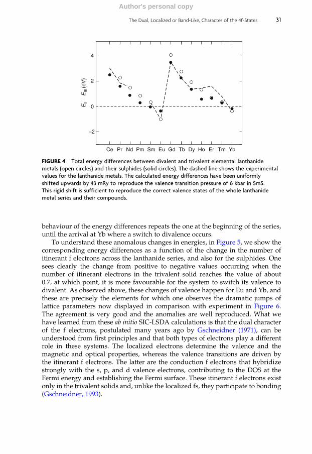
behaviour of the energy differences repeats the one at the beginning of the series,until the arrival at Yb where a switch to divalence occurs.

To understand these anomalous changes in energies, in Figure 5, we show thecorresponding energy differences as a function of the change in the number ofitinerant f electrons across the lanthanide series, and also for the sulphides. Onesees clearly the change from positive to negative values occurring when thenumber of itinerant electrons in the trivalent solid reaches the value of about0.7, at which point, it is more favourable for the system to switch its valence todivalent. As observed above, these changes of valence happen for Eu and Yb, andthese are precisely the elements for which one observes the dramatic jumps oflattice parameters now displayed in comparison with experiment in Figure 6.The agreement is very good and the anomalies are well reproduced. What wehave learned from these ab initio SIC-LSDA calculations is that the dual characterof the f electrons, postulated many years ago by Gschneidner (1971), can beunderstood from first principles and that both types of electrons play a differentrole in these systems. The localized electrons determine the valence and themagnetic and optical properties, whereas the valence transitions are driven bythe itinerant f electrons. The latter are the conduction f electrons that hybridizestrongly with the s, p, and d valence electrons, contributing to the DOS at theFermi energy and establishing the Fermi surface. These itinerant f electrons existonly in the trivalent solids and, unlike the localized fs, they participate to bonding(Gschneidner, 1993).

Ce

−2

0

2

4

Ell

− E

lll (e

V)

YbTmErHoDyTbGdEuSmPmNdPr

FIGURE 4 Total energy differences between divalent and trivalent elemental lanthanide

metals (open circles) and their sulphides (solid circles). The dashed line shows the experimental

values for the lanthanide metals. The calculated energy differences have been uniformly

shifted upwards by 43 mRy to reproduce the valence transition pressure of 6 kbar in SmS.

This rigid shift is sufficient to reproduce the correct valence states of the whole lanthanide

metal series and their compounds.



4.3 Valence of pnictides and chalcogenides

At ambient conditions, the lanthanidemonopnictides RX (X¼N, P, As, Sb, Bi) andmonochalcogenides RX (X ¼ 0, S, Se, Te, Po) crystallize in the NaCl structure.Given the combination of an electropositive R-ion with an electronegative pnic-tide or chalcogenide, one might assume that an ionic picture can be applied here.But based on the observed properties, Rhyne and McGuire (1972) proposed aclassification distinguishing between the so-called valence balanced compoundsPnictide3�R3þ , Chalcogenide2�R2þ , and valence unbalanced compounds such as

Ell−

Elll

(eV

)

Nflll−Nf

ll

−2

0

0 0.5 1.0

2

4

FIGURE 5 The energy differences between the divalent and trivalent valence states of the

elemental lanthanides (open circles) and their sulphides (solid circles) versus the difference

between the fractional numbers of itinerant f electrons in the two valence states.

Ce Pr Nd Pm Sm Eu Gd Tb Dy Ho Er Tm Yb3.5

4.0

S (

a.u.

)

FIGURE 6 The calculated equilibrium atomic sphere radii, S, (open circles) and their experimental

counterparts (solid circles) for all the lanthanide elements. The atomic sphere radius is defined

in the caption of Figure 1.



Chalcogenide2�R3þ . The former being mostly ionic insulators, although there areexceptions, and the latter being mostly conductors.

The overall electronic properties of the lanthanide pnictides and chalcogenidesare mainly determined by the f–f and f–d overlap between the correspondingorbitals on neighbouring lanthanide sites, and the f–p overlap between thelanthanide-sites and the pnictogen/chalcogen ion. While the f–f overlap in princi-ple leads to narrow band formation, the corresponding small gain in energy has tocompete with the strong intra-atomic correlations among the f-electrons that tendto localize them. As we will show, the difference between the valence balancedand valence unbalanced compounds is related to the competing trends off-electron localization and f-band formation. In all our calculations, we assumethe rock salt structure and ferromagnetic arrangement of spins. The reason is thatthe true magnetic structures of the lanthanide compounds are not always known.

4.3.1 The pnictidesThe lanthanide pnictides have been studied extensively, given their potentialapplications. An overview of their electronic and magnetic properties has recentlybeen written by Duan et al. (2007). An earlier review of the lanthanide pnictidescan be found in Hulliger (1979). In this section, we shall mainly concentrate on thevalencies of the lanthanide-ions, and the resulting electronic structure, as obtainedwithin the SIC-LSD approach. In a simple ionic picture, one expects the pnictidesto be trivalent insulators. The reason being that the pnictide ion, when alloyedwith the lanthanide element, can accommodate additional three electronsthrough charge transfer and hybridization. The resulting trivalent lanthanide-ionconfiguration is confirmed by experiment and the present calculations. Many ofthese compounds, however, turn out not to be insulators.

Among the nitrides, only NdN, GdN, TbN, and DyN definitely order ferro-magnetically, SmN is anti-ferromagnetic, and most of the remaining nitrides havenot been investigated in sufficient detail for their magnetic structure to be unam-biguously defined. The SIC-LSD study of the lanthanide–nitrides in the ferromag-netically ordered state finds all the compounds, from Pr onwards, to be trivalentin the ground state (Aerts et al., 2004). CeN is found to prefer, energetically, thetetravalent configuration. The calculated energy difference, EII�EIII, between thedivalent and trivalent configurations, is shown in Figure 7. As expected, the trendis towards a strongly trivalent state at the beginning of the series, and a decreasingenergy difference as a function of filling up the f-shell up to Eu. Trivalent Gd isagain very energetically favourable, given the half-filled f-shell, after which theenergy trend repeats itself. The divalent configuration, however, does not becomefavourable for any of the nitrides. The calculated lattice parameters (Aerts et al.,2004) are compared to the experimental values (Wyckoff, 1968) in Figure 8. Thejump between Ce and Pr is due to the valence change from tetravalent to trivalent.The overall agreement is very good, even though for some of the lighter lantha-nides, the unexplained irregularities in the experimental data seem to reflect therelatively limited quality of the samples available at the time.

In Table 2, we show the spin-resolved band gaps and densities of states of eachmaterial at the Fermi energy. It is clear from the table that our SIC-LSD



calculations find most of the light lanthanide nitrides to be half-metallic. OnlyCeN is metallic because it exists in the tetravalent state (in fact the trivalent state isalso just metallic). TbN, DyN, and HoN are found to be narrow band gapinsulators, and ErN, TmN, and YbN are metallic in both spin-channels, with theFermi energy lying at the bottom of the spin-down 4f-states, leading to a ratherlarge spin-down DOS at the Fermi energy. The insulating (semi-conducting), half-metallic, and full metallic behaviours that we have predicted for lanthanidenitrides is a consequence of the nitrogen p and the band-like lanthanide f-statesoccurring in the same energy window, in the vicinity of the Fermi level, whichleads to strong hybridization of these states. Our results seem to suggest thatlanthanide nitrides and their alloys may enable us to fabricate materials with awide and continuous range of useful properties, particularly with regard to spinfiltering applications where they may provide alternatives to the lanthanidechalcogenides already in use for this purpose (Moodera et al., 1993; Worledgeand Geballe, 2000; Filip et al., 2002; LeClair et al., 2002).

The total and species-decomposed spin magnetic moments are displayed inTable 3. There we also present the lanthanide orbital moments. With the excep-tions of ErN, TmN, and YbN, the spin magnetic moments of these materials takeon an integer value. This indicates that these systems are either insulating(Tb-, Dy-, and Ho-nitrides) or half-metallic (Pr- to Gd-nitrides), since one needsat least one full band in one of the spin channels to obtain an integer value forthe spin magnetic moment. CeN is a non-magnetic metal, and the last threecompounds of the series are metallic in both spin-channels. These results are asone would expect; the spin magnetic moment is dominated by the rare earthf-electrons, with some hybridization yielding small contributions from the rare

Ce

Ell–

Elll (

eV)

–2

–1

0

1

2

3

4

5

6

7

8 R

RN


FIGURE 7 Total energy differences (in eV) between divalent and trivalent scenarios for

lanthanide nitrides (triangles). The results for elemental lanthanides (diamonds) are repeated

for an easy comparison (including 43 mRy correction, but not for the nitrides).



Ce9.0

9.2

9.4

9.6

a (

a.u.

)

9.8

10.0


FIGURE 8 Lattice parameters of the lanthanide nitrides. The open circles are the experimental

values, whereas the solid circles are the calculated lattice parameters.

TABLE 2 Spin-resolved band gaps (in Ry) and densities of states (in states/Rydberg/formula unit)

at the Fermi energy for the lanthanide nitrides

Material

Band gap DOS

Spin up Spin down Spin up Spin down

CeN 0 0 15.37 15.37

PrN 0 0.039 0.0001 0NdN 0 0.065 0.068 0PmN 0 0.076 31.77 0SmN 0 0.095 154.56 0EuN 0 0.107 69.85 0GdN 0 0.082 0.065 0

TbN 0.008 0.052 0 0DyN 0.018 0.058 0 0HoN 0.031 0.004 0 0

ErN 0 0 0.682 69.57TmN 0 0 1.52 220.78YbN 0 0 1.72 93.18



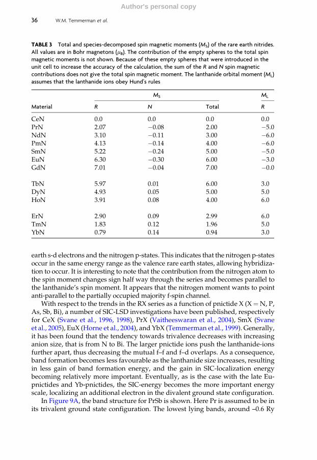
earth s-d electrons and the nitrogen p-states. This indicates that the nitrogen p-statesoccur in the same energy range as the valence rare earth states, allowing hybridiza-tion to occur. It is interesting to note that the contribution from the nitrogen atom tothe spin moment changes sign half way through the series and becomes parallel tothe lanthanide’s spin moment. It appears that the nitrogen moment wants to pointanti-parallel to the partially occupied majority f-spin channel.

With respect to the trends in the RX series as a function of pnictide X (X¼N, P,As, Sb, Bi), a number of SIC-LSD investigations have been published, respectivelyfor CeX (Svane et al., 1996, 1998), PrX (Vaitheeswaran et al., 2004), SmX (Svaneet al., 2005), EuX (Horne et al., 2004), and YbX (Temmerman et al., 1999). Generally,it has been found that the tendency towards trivalence decreases with increasinganion size, that is from N to Bi. The larger pnictide ions push the lanthanide-ionsfurther apart, thus decreasing the mutual f–f and f–d overlaps. As a consequence,band formation becomes less favourable as the lanthanide size increases, resultingin less gain of band formation energy, and the gain in SIC-localization energybecoming relatively more important. Eventually, as is the case with the late Eu-pnictides and Yb-pnictides, the SIC-energy becomes the more important energyscale, localizing an additional electron in the divalent ground state configuration.

In Figure 9A, the band structure for PrSb is shown. Here Pr is assumed to be inits trivalent ground state configuration. The lowest lying bands, around –0.6 Ry

TABLE 3 Total and species-decomposed spin magnetic moments (MS) of the rare earth nitrides.

All values are in Bohr magnetons (mB). The contribution of the empty spheres to the total spin

magnetic moments is not shown. Because of these empty spheres that were introduced in the

unit cell to increase the accuracy of the calculation, the sum of the R and N spin magnetic

contributions does not give the total spin magnetic moment. The lanthanide orbital moment (ML)

assumes that the lanthanide ions obey Hund’s rules

Material

MS ML

R N Total R

CeN 0.0 0.0 0.0 0.0PrN 2.07 �0.08 2.00 �5.0NdN 3.10 �0.11 3.00 �6.0PmN 4.13 �0.14 4.00 �6.0SmN 5.22 �0.24 5.00 �5.0EuN 6.30 �0.30 6.00 �3.0GdN 7.01 �0.04 7.00 �0.0

TbN 5.97 0.01 6.00 3.0DyN 4.93 0.05 5.00 5.0HoN 3.91 0.08 4.00 6.0

ErN 2.90 0.09 2.99 6.0TmN 1.83 0.12 1.96 5.0YbN 0.79 0.14 0.94 3.0



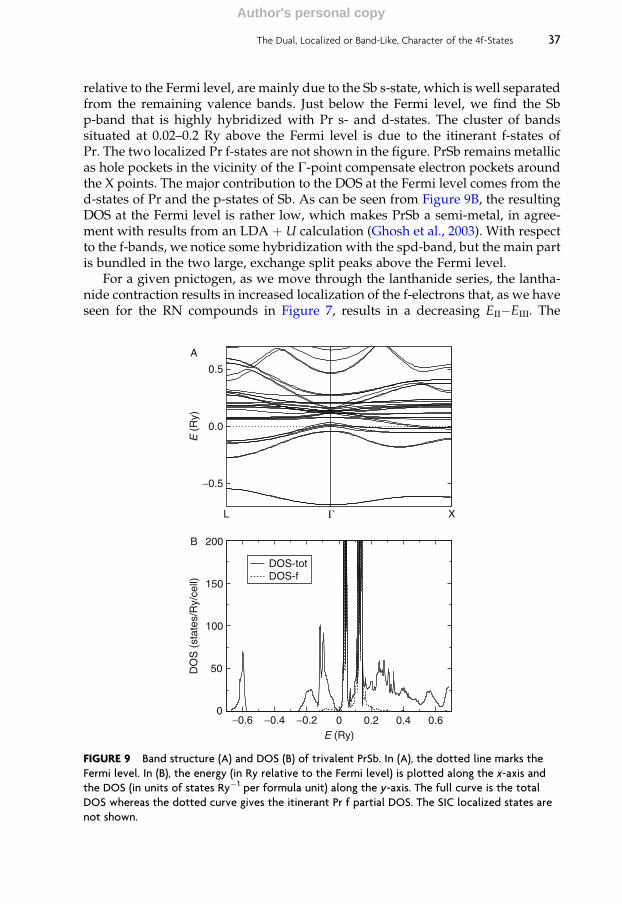
relative to the Fermi level, are mainly due to the Sb s-state, which is well separatedfrom the remaining valence bands. Just below the Fermi level, we find the Sbp-band that is highly hybridized with Pr s- and d-states. The cluster of bandssituated at 0.02–0.2 Ry above the Fermi level is due to the itinerant f-states ofPr. The two localized Pr f-states are not shown in the figure. PrSb remains metallicas hole pockets in the vicinity of the G-point compensate electron pockets aroundthe X points. The major contribution to the DOS at the Fermi level comes from thed-states of Pr and the p-states of Sb. As can be seen from Figure 9B, the resultingDOS at the Fermi level is rather low, which makes PrSb a semi-metal, in agree-ment with results from an LDA þ U calculation (Ghosh et al., 2003). With respectto the f-bands, we notice some hybridization with the spd-band, but the main partis bundled in the two large, exchange split peaks above the Fermi level.

For a given pnictogen, as we move through the lanthanide series, the lantha-nide contraction results in increased localization of the f-electrons that, as we haveseen for the RN compounds in Figure 7, results in a decreasing EII�EIII. The

X�L

−0.5

0.0

E (

Ry)

0.5

A

B

0−0.6

E (Ry)0.2 0.4

50

100

150

DO

S (

stat

es/R

y/ce

ll)

200

DOS-totDOS-f

0.60−0.2−0.4

FIGURE 9 Band structure (A) and DOS (B) of trivalent PrSb. In (A), the dotted line marks the

Fermi level. In (B), the energy (in Ry relative to the Fermi level) is plotted along the x-axis and

the DOS (in units of states Ry�1 per formula unit) along the y-axis. The full curve is the total

DOS whereas the dotted curve gives the itinerant Pr f partial DOS. The SIC localized states are

not shown.



increasing trend towards localization also means that the corresponding f-stateenergy levels move towards lower energies, that is they move closer to thepnictogen p-band. This can be observed, for example, in the previously describedPrSb DOS depicted in Figure 9B, as compared with the DOS of SmAs shown inFigure 10. In the latter, we find two narrow Sm f resonances situated just above theFermi level. With increasing localization of the lanthanide ion f-electrons, theitinerant f-peak gets pinned to the Fermi level, and as theymove to lower energies,they start filling up with valence electrons. It was shown earlier that the degreeof populating the delocalized narrow f-peak is correlated with EII�EIII, in thesense that the SIC energy is related to the occupied f-states and becomes increas-ingly important as the f-peak is being occupied, eventually preferring to localize.Thus, the increased occupancy of the f-peak explains the observed trend invalence as a function of lanthanide ion.

Parallel to the observed trend towards filling up the f-peak as a function of thelanthanide ion, one also observes increased occupancy for a given lanthanide asonemoves through the pnictide series fromN to Bi. Again this can be correlated tothe corresponding EII�EIII. In the Sm pnictides, for example, the preference for atrivalent ground state configuration is reduced from 135 mRy per formula unit inSmN to only 6 mRy per formula unit in SmBi (Svane et al., 2005). This trend isexplained by the fact that with decreasing electronegativity, the p-bands move upin energy, which results in the Fermi energy moving progressively into the f-peakwhen going from N to Bi. As this happens, the pnictide p-bands are intersected atthe top by the narrow f-band which pins the Fermi level.

The two trends of f-peak moving towards lower energies with increasingf-electron localization, and of the p-band moving towards higher energies withdecreasing electronegativity, culminate for the Eu pnictides and Yb pnictides,and the resulting large degree of occupancy of the f-peak means that the gain in

−12

E (eV)

0

2

4

6

8

DO

S (

stat

es/e

V/c

ell)

40−4−8

FIGURE 10 DOS with respect to the Fermi energy of trivalent SmAs. The full line shows the total

DOS and the dotted line shows the Sm contribution. The SIC localized states are not shown.



SIC-energy becomes large enough to overcome the loss in band formation energy.Thus, from the calculated EII�EIII, we observe that this energy difference eventu-ally turns marginally positive or even negative for the later Eu pnictides, EuAs,EuSb, and EuBi, and YbBi. These findings are in good agreement with experiment,where it turns out that neither of the latter compounds exists in the NaCl structure(Iandelli and Franceschi, 1973), and one might speculate that this is due to the factthat the trivalent configuration is no longer stable in these compounds. Thus,EuAs adopts the hexagonal Na2O2 crystal structure (Ono et al., 1971; Wang et al.,1977), that is a distortion of the NiAs structure due to the formation of anion–anion pairs. In conclusion, although the large majority of the lanthanide pnictidesprefer the trivalent ground state configuration, the trend towards trivalencedecreases with cation size from Ce to Eu, and again from Gd to Yb, as well aswith anion size from N to Bi. In the Eu series, the N and P are still sufficientlyelectronegative to support the charge transfer of three electrons resulting in Eu3 þ

ions, but starting with EuAs, seven f-electrons remain localized at the Eu site, andan eventual NaCl structure, with divalent Eu ions, is unstable to structuraltransition towards the Na2O2 crystal structure.

4.3.2 The chalcogenidesIn many respects, the chalcogenides are similar to the pnictides, crystallizing inthe same NaCl structure and with the s-, p-, and d-states situated at the sameenergy ranges as their corresponding neighbours to the left in the Periodic Table.Nevertheless, with respect to the electronic structure, they differ dramaticallyfrom each other, which can be traced to the fact that with one additionalp-electron, there is only space for accommodating two additional electrons inthe valence band, through charge transfer and hybridization. As a consequence,an eventual trivalent ground state is forced to accommodate the third electron inthe narrow f-peak, which results in many more compounds being situated at theboundary of the trivalent–divalent phase transition. A divalent ground stateconfiguration is in agreement with the ionic picture for chalcogenides.

Calculations with the SIC-LSD method of the lanthanide-sulphides (Strangeet al., 1999) have shown that divalence already sets in here, although only withrespect to the lanthanide ions Sm, Eu, and Yb, as can be seen from Figure 11. At thebeginning of the lanthanide series, the empty f-levels are held well above theFermi level, and the third electron is accommodated in the states at the bottom ofthe broad sd-band. As the atomic number increases, the f-levels move closer to theFermi level and start picking up electrons. As we reach SmS, the state immediatelyabove the Fermi level is almost entirely of f character, and the electrons now fillingup the narrow peak prefer to localize, resulting in a divalent ground state. Thisbehaviour occurs in the light lanthanide from CeS to EuS, and is repeated in theheavy lanthanide from GdS to YbS.

For the lanthanide chalcogenides, it was demonstrated experimentally thatSm, Eu, and Yb are divalent in their sulphide, selenide, and telluride compounds,while Tm becomes divalent for the telluride phase only ( Jayaraman, 1978, 1979).The SIC-LSD calculations find all the Eu chalcogenides, including EuO, to beinsulators in the ferromagnetic state, and to have a divalent configuration



(Horne et al., 2004). For the Yb chalcogenides, the divalent state is seen to befavoured in all cases by 35–70 mRy (Svane et al., 2000). Both of these results arethus in good agreement with experiment. With respect to the Sm chalcogenidesalready in Smmonoxide, the divalent f 6 configuration is found to be energeticallymost favourable, by 6 mRy, and in SmS by 15 mRy (Svane et al., 2005). Hence, theSIC-LSD predicts a Sm valence transition between the pnictides and chalcogen-ides, as shown in Figure 12. This is not in complete agreement with the experi-mental picture, according to which the divalent and trivalent ground states in SmSare almost degenerate, while Sm in SmO is trivalent and metallic (Krill et al., 1980;Leger et al., 1980). Thus, it appears that the SIC-LSD functional overestimates thetendency for divalence by approximately 15 mRy in SmS. Assuming this error tobe similar for all SmX compounds, this would imply that the calculated energybalance curve in Figure 12 lies too high by approximately 15 mRy. In Figure 12, wetherefore include a calibrated energy curve (dashed line) when 15 mRy correctionis subtracted from the calculated trivalent-divalent energy difference. In the paperby Strange et al. (1999), a similar uniform calibration of 43 mRy (this uniformenergy shift is already included in Figure 11) was applied to the trivalent-divalentenergy difference of the lanthanide sulphides in order to account for the experi-mentally observed valence of SmS. The different size of the calibrating energyshift can to a large extent be traced to the neglect of spin-orbit coupling in theformer work of Strange et al. (1999).

In the Tm chalcogenides, the calculated energy differences between divalentf 13 and trivalent f 12 are found to be �1.2, �13.5, �24.3, and �37.3 mRy for TmS,

Ce Pr Nd Pm Sm Eu Gd Tb Dy Ho Er Tm Yb−2

0

2

4

6

R

RS

8

E

ll−E

lll (e

V)

FIGURE 11 Total energy differences (in eV) between divalent and trivalent scenarios for

lanthanide sulphides (squares). The results for elemental lanthanides (diamonds) are repeated

for an easy comparison (including 43 mRy correction also applied to sulphides).



TmSe, TmTe, and TmPo, respectively, reflecting the trend towards greater locali-zation with the larger ligand. Also here, it turns out that at ambient pressure, thetrend towards localization is overestimated by some 15 mRy, as it is foundexperimentally that TmS is a trivalent metal and TmSe is in a mixed valent state.

4.4 Valence of ytterbium compounds

Ytterbium compounds show a wealth of anomalous physical phenomena causedby the intricate electronic structure related to its f-electrons (Cho et al., 1993;Wachter, 1993; Joyce et al., 1996). In the atomic ground state, Yb is divalent witha filled f 14 shell, but in the solid state, the f-electrons may play an active role in thebonding giving rise to intermediate valent, heavy-fermion, or Kondo behaviour aswell as complex magnetic structures. In Temmerman et al. (1999) and Svane et al.(2000), a number of Yb compounds were investigated with the SIC-LSD approachand the energetics of the valence of Yb ions was calculated. The divalent configu-ration is realized by applying SIC to all 14 f-electrons, while the nominallytrivalent configuration is realized by applying SIC to 13 of 14 f-electrons. In thislatter case, the last f-electron is allowed to hybridize with the normal sd conduc-tion electrons and form band states. The effective Yb valence, which is given as thenumber of non-f valence electrons, is then determined by the degree of occupancyof these f-band states, and the resulting electronic structure may be viewed as arealization of an intermediate valence state. The highest effective valence found inthis study is 2.88 (for YbN), that is, in no case is the ideal trivalent state reached.The results are summarized in Figure 13 that shows the energy difference betweenthe two localization scenarios correlated with the degree of filling of the f-band inthe nominally trivalent scenario.

N−150

−100 SmX

−50E

lll−E

ll (m

Ry)

0

50

PoTeSeSOBiSbAsP

FIGURE 12 Total energy differences (in mRy) between divalent and trivalent scenarios for

SmX (full line). A negative sign implies that the trivalent state is favoured. The dashed line

marks a 15 mRy corrected energy curve: this is the amount by which the SIC-LSD (with spin-orbit

included) overestimates the tendency to form the divalent configuration.



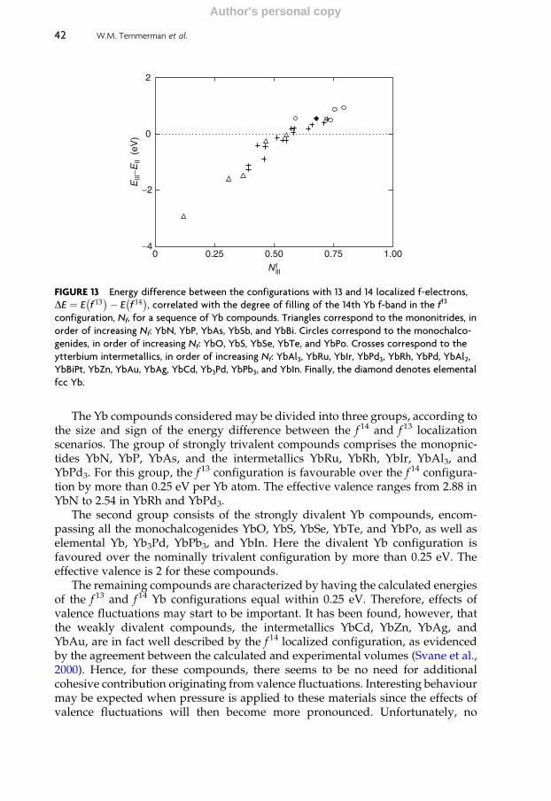
The Yb compounds considered may be divided into three groups, according tothe size and sign of the energy difference between the f 14 and f 13 localizationscenarios. The group of strongly trivalent compounds comprises the monopnic-tides YbN, YbP, YbAs, and the intermetallics YbRu, YbRh, YbIr, YbAl3, andYbPd3. For this group, the f 13 configuration is favourable over the f 14 configura-tion by more than 0.25 eV per Yb atom. The effective valence ranges from 2.88 inYbN to 2.54 in YbRh and YbPd3.

The second group consists of the strongly divalent Yb compounds, encom-passing all the monochalcogenides YbO, YbS, YbSe, YbTe, and YbPo, as well aselemental Yb, Yb3Pd, YbPb3, and YbIn. Here the divalent Yb configuration isfavoured over the nominally trivalent configuration by more than 0.25 eV. Theeffective valence is 2 for these compounds.

The remaining compounds are characterized by having the calculated energiesof the f 13 and f 14 Yb configurations equal within 0.25 eV. Therefore, effects ofvalence fluctuations may start to be important. It has been found, however, thatthe weakly divalent compounds, the intermetallics YbCd, YbZn, YbAg, andYbAu, are in fact well described by the f 14 localized configuration, as evidencedby the agreement between the calculated and experimental volumes (Svane et al.,2000). Hence, for these compounds, there seems to be no need for additionalcohesive contribution originating from valence fluctuations. Interesting behaviourmay be expected when pressure is applied to these materials since the effects ofvalence fluctuations will then become more pronounced. Unfortunately, no

0−4

−2

0

2

Elll−E

ll (

eV)

0.25

N flll

1.000.750.50

FIGURE 13 Energy difference between the configurations with 13 and 14 localized f-electrons,

DE ¼ E f 13� �

� E f 14� �

, correlated with the degree of filling of the 14th Yb f-band in the f13

configuration, Nf, for a sequence of Yb compounds. Triangles correspond to the mononitrides, in

order of increasing Nf: YbN, YbP, YbAs, YbSb, and YbBi. Circles correspond to the monochalco-

genides, in order of increasing Nf: YbO, YbS, YbSe, YbTe, and YbPo. Crosses correspond to the

ytterbium intermetallics, in order of increasing Nf: YbAl3, YbRu, YbIr, YbPd3, YbRh, YbPd, YbAl2,

YbBiPt, YbZn, YbAu, YbAg, YbCd, Yb3Pd, YbPb3, and YbIn. Finally, the diamond denotes elemental

fcc Yb.



pressure experiments have been reported on any of the Yb compounds in thisgroup. Finally, the compounds YbSb, YbBi, YbBiPt, YbPd, and YbAl2 are weaklytrivalent, that is according to the calculations, the f 13 localization scenario isfavoured by less than 0.25 eV. Among these, YbBiPt and YbAl2 are known to beheavy-fermion compounds (Havinga et al., 1973; Robinson et al., 1994), and YbPdis believed to be a mixed valent system, with approximately equal proportions ofYb2þ and Yb3þ ions (Iandelli et al., 1980; Bonville et al., 1986). YbBi has never beensynthesized, while YbSb in most respects resembles the other predominantlytrivalent Yb pnictides, however, with somewhat unusual low-temperature mag-netic behaviour (Kasuya, 1994; Oyamada et al., 1994; Li et al., 1995). Hence, for thecompounds in this group, the valence fluctuation phenomena seem to be signifi-cant. The calculated effective valencies range from 2.53 in YbSb to 2.45 in YbBi andYbBiPt, that is, the band states of the 14th f-electron are approximately half-filled.The heavy-fermion character of YbBiPt is also confirmed by LDAþU calculations(Oppeneer et al., 1997).

In conclusion, the valence classification of Yb compounds, based on the SIC-LSD total energies, maps very well onto the physical properties observed experi-mentally. In particular, this allows to identify the third group of compounds as theheavy-fermion and mixed-valent systems on the trivalent side, and, on the diva-lent side, those systems that are likely to undergo pressure-induced valencetransitions.

At ambient conditions, theYbmonopnictides andmonochalcogenides crystallizein the B1 structure.As outlined, theYbpnictides are all found to bewell described bythe nominally trivalent scenario, where the effective valence varies from 2.88 in YbNto 2.69, 2.63, and 2.53 in YbP, YbAs, and YbSb, respectively. Experimentally, theposition of the f 14 band is found �0.2 eV above the Fermi level in YbN, YbP, andYbAs (Degiorgi et al., 1990, 1993). Other experiments have revealed heavy-electronbehaviour in Yb pnictides (Ott et al., 1985; Sakon et al., 1992; Takeda et al., 1993), butthis can be a reflection of sample non-stoichiometry (Degiorgi et al., 1990, 1993). Thediscrepancy between the present electronic structure and the picture provided byDegiorgi et al. (1990, 1993) can bedue to the LSDapproximation, since the position ofthe narrow f14 band in the theory is solely determined by the LSD potential(no correlation correction).LDAþU calculationsonYbN (Larsonet al., 2007) includea positive correlation shift of the unoccupied f-states that leads to an ideal trivalentYb ion in accordance with Degiorgi et al. (1990, 1993).

In contrast to the pnictides, the equilibriumvolumes of theYb chalcogenides areaccurately described assuming the divalent f 14 configuration for Yb. As pressure isapplied to the Yb chalcogenides, the f 13 configuration becomes more and morefavourable, and eventually a transition to an intermediate valence state occurs.Valence transitions in lanthanide systems will be discussed in the next section.

4.5 Valence transitions

When pressure is applied to lanthanide systems, the interaction of the electronsgenerally increases and at some point, it becomes advantageous for the f-electronsto contribute more actively to the bonding, that is the effective valence increases.



In the SIC-LSD formalism, this happens when localization scenarios of different fn

configurations become close in energy. In the present T ¼ 0 K theory, onlydiscontinuous pressure-induced transitions can be described, while experimentsoften, but not always, observe continuous transitions, signalled by anomaloussoftening of the pV-curve.

Tables 4 and 5 summarize results for valence transitions in the cerium andpraseodymium pnictides (Svane et al., 1996, 1998; Vaitheeswaran et al., 2004) andselected rare earth chalcogenides (Svane et al., 1998, 1999, 2001, 2004;Vaitheeswaran et al., 2004; Lebegue et al., 2005; Svane et al., 2005). In Figure 14is shown the total energy of CeP as calculated with SIC-LSD considering both theB1 (rocksalt) and B2 (caesium chloride) crystal structures as well as both theitinerant, f 0, and the localized, f 1, scenario for the Ce ions (Svane et al., 1996).The lowest energy is found in the B1 phase with localized f-electrons and with aspecific volume of 348 a30 per formula unit, which coincides with the experimentalequilibrium volume. The B1 phase with delocalized f-electrons has its minimumat a considerably lower volume, due to the significant f-electron band formationenergy providing a large negative component to the pressure. From the commontangent, a phase transition is predicted at a pressure of 7.1 GPa with a volumecollapse of DV/V0 ¼ 8% (change in volume relative to the zero pressure equilib-rium volume), which is in excellent agreement with the transition observed at 5.5GPa (Mori et al., 1993). The B2 structure is not as favourable for the CeP com-pound since the calculated energy is substantially higher than that of the B1structure. This holds for both localized and delocalized f-electrons. FromFigure 14, we conclude that the B2 structure with localized f-electrons is neverreached in CeP, while at high pressure, a second phase transition to the B2 struc-ture with delocalized f-electrons is found. The transition pressure is calculated tobe 11.3 GPa and the volume collapse 12%, while experimentally, the B1 ! B2phase transition is seen at 15 � 4 GPa (Vedel et al., 1987). The experimentalvolume collapse is 11%.

The results reported in Table 4 show that all of the observed pressure transi-tions in the cerium pnictides and chalcogenides are indeed reproduced (Svaneet al., 1998). In all cases except CeN is the localized f 1 configuration favoured inthe ground state. The total energy curves look rather similar to those of CeP inFigure 14, but minor changes in the relative positions occur when the ligand isvaried. The localized phases are generally more favoured when the ligand ionbecomes heavier, and as a consequence, in CeAs, no isostructural delocalizationtransition occurs in the B1 structure. Instead, a transition directly from the B1structure with localized f-electrons to the B2 structure with delocalized f-electronsoccurs, in agreement with experiment. In CeSb and CeBi, the first high-pressuretransition to occur is from B1 to B2, with localized f-electrons in both cases, andonly at higher pressures is a delocalization transition predicted to take place. Thecalculated transition pressures for these delocalization processes are only slightlyabove the ranges studied experimentally. In this work, only the B2 structure wasconsidered for the second transition, but in reality, the valence transition whicheventually must take place in CeSb and CeBi may involve another unknown highpressure phase.



In CeS, the first transition occurs to the B1 phase with delocalized f-electrons(Svane et al., 1999), that is, the theory predicts an isostructural phase transition inCeS similar to CeP. The calculated transition pressure is 10.1 GPa with a volumecollapse of 6%. These findings are in excellent agreement with the experiment ofCroft and Jayaraman (1980), but at variance with the results of Vedel et al. (1986),who observe a soft anomaly in the pV-curve but no discontinuity. These resultsmay indicate the proximity of a critical point. At higher pressures, CeS transformsinto the B2 phase. According to the present calculations, this occurs in two steps.First, at a pressure of 24.3 GPa, CeS goes into the trivalent B2 phase with a 4.6%volume change. In the second step, at a pressure of 29.5 GPa, the tetravalent B2phase is reached with a 3.6% volume collapse (Svane et al., 1999). Unfortunately,no experiments have been performed beyond 25 GPa (Leger, 1993).

In both CeSe and CeTe, the only pressure transition observed is that from B1 toB2 with localized f-electrons in both phases. These are also first to occur accordingto the calculations, whereas valence transitions are predicted in the range of 40GPa. Thus, the situation here is quite similar to that in CeSb and CeBi, apart fromthe tetragonal distortion in these compounds that was not found for CeSe and

TABLE 4 Calculated transition pressures for the electronic and structural phase transitions in the

Ce pnictides and chalcogenides. Also quoted are the volume discontinuities (relatively to the zero

pressure equilibrium volume) at the transition. The notation ( f n) refers to SIC-LSD calculations

with n localized f-electrons. For the cerium pnictides, B2* denotes the distorted B2 structure.

Experimentally, the transitions of the Ce pnictides are discontinuous, while those of the cerium

chalcogenides (at room temperature) are continuous

Compound Transition

Pt (GPa) Volume collapse (%)

Theoretical Experimental Theoretical Experimental

CeN B1( f 0)!B2( f 0) 62.0 – 3.6 –CeP B1( f 1)!B1( f 0) 7.1 9.0a,5.5b 8.0 4a

CeP B1( f 0)!B2( f 0) 11.3 15(4)a,25.0j 12.1 11a

CeAs B1( f 1)!B2( f 0) 11.4 14(2)c,21.0j 18.0 11c

CeSb B1( f 1)!B2*( f 1) 7.0 8.5(2.5)d,15j 10.9 10d

CeSb B2*( f 1)!B2*( f 0) 25.2 – 3.7 –CeBi B1( f 1)!B2*( f 1) 8.8 9(4)e 10.8 9e

CeBi B2*( f 1)!B2*( f 0) 37.0 – 2.8 –CeS B1( f 1)!B1( f 0) 10.1 –f,12.5(1.5)g 6.3 5g

CeS B1( f 0)!B2( f 1) 24.3 – 4.6 –CeS B2( f 1)!B2( f 0) 29.5 – 3.6 –CeSe B1( f 1)!B2( f 1) 12.4 17(3)h 11.1 9h

CeSe B2( f 1)!B2( f 0) 37.7 – 3.1 –CeTe B1( f 1)!B2( f 1) 74.0 5.5(2.5)i 11.7 9i

CeTe B2( f 1)!B2( f 0) 43.5 – 2.4 –

a Vedel et al. (1987); b Mori et al. (1993); c Werner et al. (1983); d Leger et al. (1984); e Leger et al. (1985); f Leger (1993);g Croft and Jayaraman (1980); h Leger and Redon (1989); i Leger et al. (1983).



CeTe. The B1 ! B2 transition in cerium chalcogenides has also been investigatedwithin the GGA approach (Bouhemadou et al., 2005), in which case, the f electronsare treated as itinerant.

The SIC-LSD studies on the Pr chalcogenides and pnictides show that theground state favours the B1 structure over the B2 structure throughout the entireseries. With applied pressure, all these compounds undergo a transition to the B2CsCl structure (or a distorted version of it). For the Pr pnictides, the calculatedtransition pressures agree quite well with experiment, although they are

TABLE 5 Calculated transition pressures for the electronic and structural phase transitions in

the Pr pnictides and chalcogenides of Pr, Sm, Eu, Tm, and Yb. Also quoted are the volume

discontinuities (relatively to the zero pressure equilibrium volume) at the transition. The notation

( f n ) refers to SIC-LSD calculations with n localized f-electrons. Experimentally, the transitions

of SmS are discontinuous, while those of SmSe, SmTe, EuO, EuS, and the Tm and Yb chalcogenides

(at room temperature) are continuous. The volume changes for SmSe and SmTe as well as TmTe

are obtained by extrapolation over the transition range. For Yb compounds, we quote the relative

volumes at which the delocalization starts

Compound Transition

Pt (GPa) Volume collapse (%)

Theoretical Experimental Theoretical Experimental

PrP B1( f 2)!B2( f 2) 16.0 26a 11.4 –PrAs B1( f 2)!B2( f 2) 12.0 27a 12.4 18.4a

PrSb B1( f 2)!B2( f 2) 8.0 13a 11.7 10.0a

PrBi B1( f 2)!B2( f 2) 8.0 14a 10.9 9.0a

PrS B1( f 2)!B2( f 2) 22.0 – 8.0 –PrSe B1( f 2)!B2( f 2) 12.0 – 9.3 –PrTe B1( f 2)!B2( f 2) 5.0 9 11.7 –

SmS B1( f 6)!B1( f 5) 0.1 0.65b 1.24c 11.1 13.5b, 13.8c

SmSe B1( f 6)!B1( f 5) 3.3 �4b, 3.4c, 3–9d,2.6–4e

9.8 8b, 11d, 7e

SmTe B1( f 6)!B1( f 5) 6.2 2–8b, 5.2c, 6–8d,4.6–7.5e

8.4 9d,7e

EuO B1( f 7)!B1( f 6) 19.3 30 f, 13–30g 6.3 5 f

EuS B1( f 7)!B1( f 6) 11.6 16 h 5.7 0 h

TmSe B1( f 13)!B1( f 13) 0 0–5k 14 8 k

TmTe B1( f 13)!B1( f 13) 3.0 2–5k 15 14k

TmPo B1( f 13)!B1( f 13) 8.0 – – –YbO B1( f 14)!B1( f 13) 18.0 8i 0.87 0.95i

YbS B1( f 14)!B1( f 13) 7.5 10j 0.93 0.88j

YbSe B1( f 14)!B1( f 13) 16.0 15f 0.79 0.75f

YbTe B1( f 14)!B1( f 13) 24.0 15f 0.78 0.65f

a Shirotani et al. (2003); b Benedict and Holzapfel (1993); c Insulator-metal transition of Sidorov et al. (1989); d Presentauthor’s estimates from figures of Bihan et al. (1995) and e Tsiok et al. (1991); f Jayaraman et al. (1974); g Zimmer et al.(1984); h Insulator-metal transition, Syassen (1986). i Werner et al. (1981); j Syassen (1986). k Debray et al. (1982).



systematically lower, as can be seen from Table 5. The agreement with experimentis equally good for PrTe, while the values for PrS and PrSe have not yet beenmeasured experimentally. Unlike in the case for the Ce pnictides and chalcogen-ides, the trivalent Pr configuration remains stable under pressure up to 50 GPa.

At ambient pressure, the Sm ions in samarium chalcogenides are divalent, f 6,but the trivalent phase becomes relevant at high pressure. In this phase, thelocalized f 5 Sm ions coexist with a partly occupied narrow f-band, effectivelydescribing an intermediate valent phase (Svane et al., 2005). The calculated andmeasured transition pressures are listed in Table 4. The good agreement both fortransition pressures and for volume collapses shows that the bonding of the high-pressure phase is well described in the SIC-LSD approximation, even if the truemany-body wavefunction of the intermediate valence phase is much more com-plicated than the corresponding SIC-LSD wavefunction. This is in line with thegeneral philosophy of the density functional approach in obtaining good totalenergy estimates from simple reference systems (non-interacting electrons). Thepresent theory cannot describe the continuous nature of the transition observedfor SmSe and SmTe. The experiments were all conducted at room temperatureand it would be interesting to investigate whether the continuous transitionwould exist at low temperature as well.

The calculated valence transition pressures for EuO and EuS in the B1 structureare compared with experiment in Table 5. Experimentally, the transition of EuO (atroom temperature) is continuous, as in SmSe and SmTe. For EuS, the experimentsshow no anomalous compression curve ( Jayaraman et al., 1974), but the band gapcloses at 16 GPa, just before the structural transition to the B2 structure occurs (at20 GPa) (Syassen, 1986). Due to the ASA in the LMTO-ASA band structure method,

200

−1.10

−1.05

−1.00E

(R

y)

−0.95B2

B1

CeP

300V (a.u.)

400

FIGURE 14 Cohesive energy of CeP (in Ry/formula unit) as a function of specific volume (in a30/

formula unit). Two crystal structures, the B1 and B2, are considered, and each with two different

treatments of the Ce f-electrons. The full drawn curves correspond to calculations with one

localized f-electron per Ce atom, whereas the dashed curves correspond to itinerant f-electrons.

The dotted line marks the common tangent at the isostructural phase transition in the B1

structure.



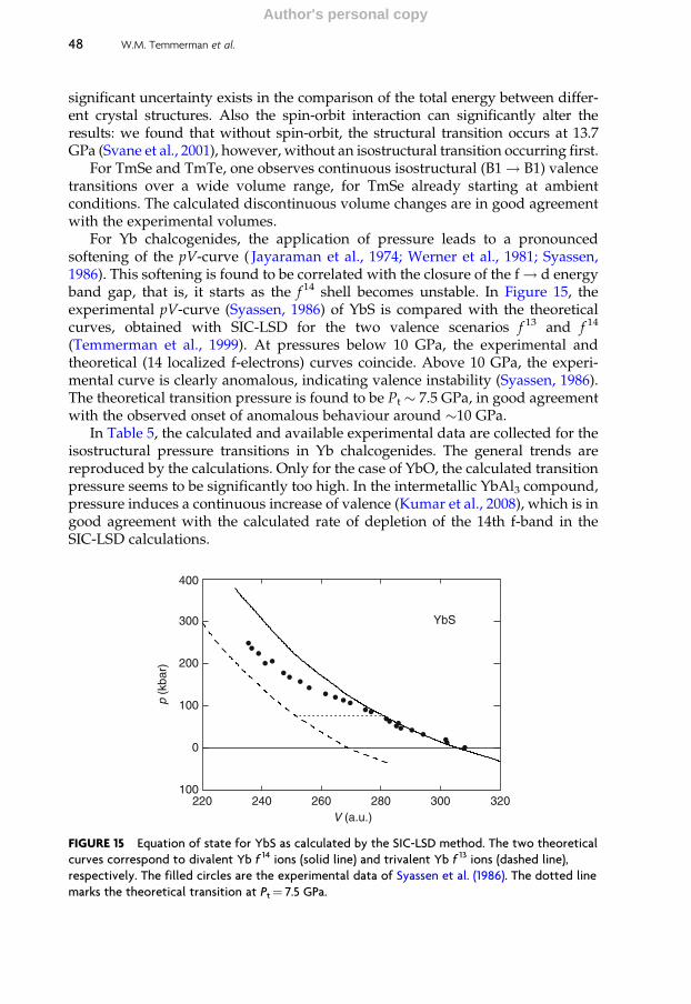
significant uncertainty exists in the comparison of the total energy between differ-ent crystal structures. Also the spin-orbit interaction can significantly alter theresults: we found that without spin-orbit, the structural transition occurs at 13.7GPa (Svane et al., 2001), however, without an isostructural transition occurring first.

For TmSe and TmTe, one observes continuous isostructural (B1! B1) valencetransitions over a wide volume range, for TmSe already starting at ambientconditions. The calculated discontinuous volume changes are in good agreementwith the experimental volumes.

For Yb chalcogenides, the application of pressure leads to a pronouncedsoftening of the pV-curve ( Jayaraman et al., 1974; Werner et al., 1981; Syassen,1986). This softening is found to be correlated with the closure of the f! d energyband gap, that is, it starts as the f 14 shell becomes unstable. In Figure 15, theexperimental pV-curve (Syassen, 1986) of YbS is compared with the theoreticalcurves, obtained with SIC-LSD for the two valence scenarios f 13 and f 14

(Temmerman et al., 1999). At pressures below 10 GPa, the experimental andtheoretical (14 localized f-electrons) curves coincide. Above 10 GPa, the experi-mental curve is clearly anomalous, indicating valence instability (Syassen, 1986).The theoretical transition pressure is found to be Pt � 7.5 GPa, in good agreementwith the observed onset of anomalous behaviour around �10 GPa.

In Table 5, the calculated and available experimental data are collected for theisostructural pressure transitions in Yb chalcogenides. The general trends arereproduced by the calculations. Only for the case of YbO, the calculated transitionpressure seems to be significantly too high. In the intermetallic YbAl3 compound,pressure induces a continuous increase of valence (Kumar et al., 2008), which is ingood agreement with the calculated rate of depletion of the 14th f-band in theSIC-LSD calculations.

220 V (a.u.)

100

0

100

200

300

400

p (

kbar

)

YbS

320300280260240

FIGURE 15 Equation of state for YbS as calculated by the SIC-LSD method. The two theoretical

curves correspond to divalent Yb f 14 ions (solid line) and trivalent Yb f 13 ions (dashed line),

respectively. The filled circles are the experimental data of Syassen et al. (1986). The dotted line

marks the theoretical transition at Pt¼ 7.5 GPa.



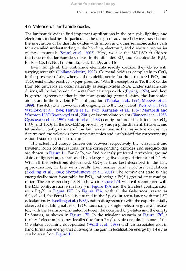
4.6 Valence of lanthanide oxides

The lanthanide oxides find important applications in the catalysis, lighting, andelectronics industries. In particular, the design of advanced devices based uponthe integration of lanthanide oxides with silicon and other semiconductors callsfor a detailed understanding of the bonding, electronic, and dielectric propertiesof these materials (Scarel et al., 2007). Here, we use the SIC-LSD to addressthe issue of the lanthanide valence in the dioxides RO2 and sesquioxides R2O3,for R ¼ Ce, Pr, Nd, Pm, Sm, Eu, Gd, Tb, Dy, and Ho.

Even though all the lanthanide elements readily oxidize, they do so withvarying strength (Holland-Moritz, 1992). Ce metal oxidizes completely to CeO2

in the presence of air, whereas the stoichiometric fluorite structured PrO2 andTbO2 exist under positive oxygen pressure. With the exception of Tb, the R-oxidesfrom Nd onwards all occur naturally as sesquioxides R2O3. Under suitable con-ditions, all the lanthanide elements form as sesquioxides (Eyring, 1978), and thereis general agreement, that in the corresponding ground states, the lanthanideatoms are in the trivalent R3þ configuration (Tanaka et al., 1995; Moewes et al.,1999). The debate is, however, still ongoing as to the tetravalent (Kern et al., 1984;Wuilloud et al., 1984; Hanyu et al., 1985; Karnatak et al., 1987; Marabelli andWachter, 1987; Boothroyd et al., 2001) or intermediate-valent (Bianconi et al., 1988;Ogasawara et al., 1991; Butorin et al., 1997) configuration of the R-ions in CeO2,PrO2, and TbO2. In the SIC-LSD approach, by studying the divalent, trivalent, andtetravalent configurations of the lanthanide ions in the respective oxides, wedetermined the valencies from first-principles and established the correspondingground state electronic structure.

The calculated energy differences between respectively the tetravalent andtrivalent R-ion configurations for the corresponding dioxides and sesquioxidesare shown in Figure 16. For CeO2, we find a clearly preferred tetravalent groundstate configuration, as indicated by a large negative energy difference of 2.4 eV.With all the f-electrons delocalized, CeO2 is thus best described in the LSDapproximation, in line with results from earlier band structure calculations(Koelling et al., 1983; Skorodumova et al., 2001). The tetravalent state is alsoenergetically most favourable for PrO2, indicating a Pr( f 1) ground state configu-ration. The corresponding DOS is shown in Figure 17B, where it is compared withthe LSD configuration with Pr( f 0) in Figure 17A and the trivalent configurationwith Pr( f 2) in Figure 17C. In Figure 17A, with all the f-electrons treated asdelocalized, the Fermi level is situated in the f-peak, in accordance with the LSDcalculations by Koelling et al. (1983), but in disagreement with the experimentallyobserved insulating nature of PrO2. Localizing a single f-electron gives an insula-tor, with the Fermi level situated between the occupied O p-states and the emptyPr f-states, as shown in Figure 17B. In the trivalent scenario of Figure 17C, afurther f-electron becomes localized to form Pr( f 2), which results in some of theO p-states becoming depopulated (Wulff et al., 1988) with an associated cost inband formation energy that outweighs the gain in localization energy by 1.4 eV ascan be seen from Figure 16.



Ce Pr Nd Pm Sm Eu Gd Tb Dy Ho

−2

0

EIV

–EIII

(eV

)

2

RO2

R2O3

FIGURE 16 Energy difference EIV–EIII (in eV per lanthanide ion) between the tetravalent and

trivalent lanthanide configurations in dioxides (solid circles) and A-type (hexagonal) sesquioxides

(open squares).

−4 −2 0E (eV)

2 4 60

5

10

15

0

5

10

15

0

5

10

15

20A

B

C

DO

S (

stat

es/e

V/c

ell)

f

f

f

0

1

2

FIGURE 17 Total DOS (solid line) and f-projected DOS (dotted line) for PrO2, with Pr in (A) the

pentavalent (f 0) configuration, (B) the tetravalent (f 1) configuration, and (C) the trivalent (f 2)

configuration. The SIC localized states are not shown. The energy is in units of eV, with zero

marking the Fermi level.



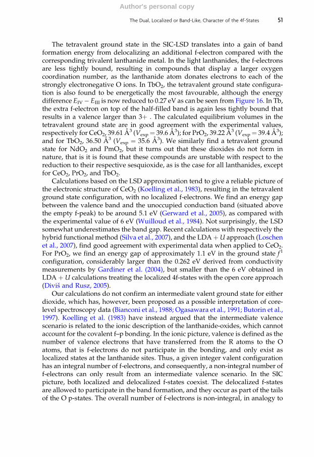
The tetravalent ground state in the SIC-LSD translates into a gain of bandformation energy from delocalizing an additional f-electron compared with thecorresponding trivalent lanthanide metal. In the light lanthanides, the f-electronsare less tightly bound, resulting in compounds that display a larger oxygencoordination number, as the lanthanide atom donates electrons to each of thestrongly electronegative O ions. In TbO2, the tetravalent ground state configura-tion is also found to be energetically the most favourable, although the energydifference EIV� EIII is now reduced to 0.27 eV as can be seen from Figure 16. In Tb,the extra f-electron on top of the half-filled band is again less tightly bound thatresults in a valence larger than 3þ . The calculated equilibrium volumes in thetetravalent ground state are in good agreement with the experimental values,respectively for CeO2, 39.61 A

3 (Vexp¼ 39.6 A3); for PrO2, 39.22 A3 (Vexp¼ 39.4 A3);

and for TbO2, 36.50 A3 (Vexp ¼ 35.6 A3). We similarly find a tetravalent groundstate for NdO2 and PmO2, but it turns out that these dioxides do not form innature, that is it is found that these compounds are unstable with respect to thereduction to their respective sesquioxide, as is the case for all lanthanides, exceptfor CeO2, PrO2, and TbO2.

Calculations based on the LSD approximation tend to give a reliable picture ofthe electronic structure of CeO2 (Koelling et al., 1983), resulting in the tetravalentground state configuration, with no localized f-electrons. We find an energy gapbetween the valence band and the unoccupied conduction band (situated abovethe empty f-peak) to be around 5.1 eV (Gerward et al., 2005), as compared withthe experimental value of 6 eV (Wuilloud et al., 1984). Not surprisingly, the LSDsomewhat underestimates the band gap. Recent calculations with respectively thehybrid functional method (Silva et al., 2007), and the LDAþU approach (Loschenet al., 2007), find good agreement with experimental data when applied to CeO2.For PrO2, we find an energy gap of approximately 1.1 eV in the ground state f 1

configuration, considerably larger than the 0.262 eV derived from conductivitymeasurements by Gardiner et al. (2004), but smaller than the 6 eV obtained inLDA þ U calculations treating the localized 4f-states with the open core approach(Divis and Rusz, 2005).

Our calculations do not confirm an intermediate valent ground state for eitherdioxide, which has, however, been proposed as a possible interpretation of core-level spectroscopy data (Bianconi et al., 1988; Ogasawara et al., 1991; Butorin et al.,1997). Koelling et al. (1983) have instead argued that the intermediate valencescenario is related to the ionic description of the lanthanide-oxides, which cannotaccount for the covalent f–p bonding. In the ionic picture, valence is defined as thenumber of valence electrons that have transferred from the R atoms to the Oatoms, that is f-electrons do not participate in the bonding, and only exist aslocalized states at the lanthanide sites. Thus, a given integer valent configurationhas an integral number of f-electrons, and consequently, a non-integral number off-electrons can only result from an intermediate valence scenario. In the SICpicture, both localized and delocalized f-states coexist. The delocalized f-statesare allowed to participate in the band formation, and they occur as part of the tailsof the O p-states. The overall number of f-electrons is non-integral, in analogy to



the intermediate valent picture, however not as a consequence of intermediatevalence but rather as a result of the p–f mixing.

At temperatures below 2000 C, the lanthanide sesquioxides adopt threedifferent structure types (Eyring, 1978). The light lanthanides crystallize in thehexagonal La2O3 structure (A-type, space group P3m1, no. 164), and the heavylanthanides assume the cubic Mn2O3 structure (C-type, Ia3, no. 206), also knownas the bixbyite structure (Villars and Calvert, 1991). Themiddle lanthanides can befound either in the C-type structure or a monoclinic distortion hereof (B-typestructure). Transitions between the different structure types are induced underspecific temperature and pressure conditions (Hoekstra and Gingerich, 1964). Weinvestigated the electronic structure of both A-type and C-type sesquioxides (Petitet al., 2005). The valence energy difference EIV � EIII for the sesquioxides in theA-type structure is displayed in Figure 16, where it can be seen that the trivalentconfiguration is the ground state in all cases. The overall trend is that of anincreasing energy difference from Ce2O3 to Gd2O3 and again from Tb2O3 toHo2O3. Apart from the extraordinary stability of the half-filled shell, which resultsin a slightly increased influence of the tetravalent configuration in Tb2O3 relativeto Gd2O3, the general tendency towards trivalence is clearly related to the increas-ing localization of the f-electrons with increasing atomic number.

A similar total energy behaviour is observed for the simulated C-type structuresesquioxides. The highly directional f-orbitals are only partially able to screeneach other from the attractive force of the nucleus, which results in a steadilyincreasing effective nuclear charge with an increasing number of f-electrons. Theincrease in localization leads to the well-known lanthanide contraction, that isthe decrease in ionic radius across the lanthanide series, which is also reflected inthe volumes of the lanthanide sesquioxide series, as illustrated in Figure 18.We notice that the agreement between theory and experiment is considerablybetter for the C-type structure than for the A-type one, which might be related tothe fact that the ASA used in the calculations is likely less reliable when applied tothe hexagonal A-type structure than when applied to the higher symmetry cubicC-type structure. Overall, for the C-type structure, the calculated values are inbetter agreement with the experimental values for the early lanthanide sesqui-oxides. This behaviour is compared in Figure 18 to the results obtained with theprojector augmented PAW (Hirosaki et al., 2003). Here the localized partly filledf-shell is treated as part of the core, which results in better agreement withexperiment for the later lanthanides with localized f-states, but which may betoo restrictive an approximation for the early lanthanide sesquioxides.

The DOS and band structures for all the sesquioxides are quite similar anddiffer mostly with respect to the unoccupied f-electron states (Petit et al., 2007). InFigure 19, we show three representative examples, namely, Eu2O3, Gd2O3, andTb2O3. The energy zero has been placed at the top of the valence bands. Thevalence band, originating from the O p-states, is of equal width (of the order of3.5 eV) in all the compounds, and is completely filled as a result of hybridizationand charge transfer. In the DOS of Eu2O3, depicted in the top panel of Figure 19, anempty f-band is situated in the gap between the valence band and the (non-f)conduction band. The low position of the f-band is caused by the exchange



interaction with the localized f 6 shell of Eu. In Gd2O3 and Tb2O3, there are onlyunoccupied minority spin f-states, and their position is significantly higher. Allthe sesquioxides, with the exception of C-type Eu2O3 are found to be insulators.

In Figure 20A, we show the evolution across the sesquioxide series of theunoccupied f-band (hatched area indicating f-band width) and the non-f conduc-tion band edge with respect to the top of the O p-bands (at zero energy). Withrespect to experimental data, in Figure 20B, one notices a considerable discrep-ancy between optical (Prokofiev et al., 1996) and conductivity (Lal and Gaur, 1988)measurements of the energy gaps. The direct comparison between theory andexperiment (Petit et al., 2005) is further complicated by the fact that in theSIC-LSD, the bare f-bands always appear at too high binding energies due to theneglect of screening and relaxation effects (Temmerman et al., 1993). The positionof the occupied and empty f-states with respect to the band edges is crucial, andthe interpretation of the optical data is that the empty f-levels are situated abovethe conduction band minimum, while the gap energies obtained from conductiv-ity measurements indicate that, for some compounds, the transitions are fromvalence ! f , that is that the empty levels can be situated in the gap betweenvalence band maximum and conduction band minimum.

From experiment, we know that whereas all the lanthanide sesquioxides canbe found in nature, the only lanthanide dioxides that occur naturally are CeO2,PrO2, and TbO2. On the other hand, SIC-LSD theory concludes that all the lantha-nide sesquioxides prefer the trivalent ground state configuration, whereas thedioxides can be separated into tetravalent light lanthanide dioxides, including

Ce70

75

80

85

90V

(Å

3 )

95

Pr Nd Pm Sm Eu Gd Dy

A-type: SIC-LSDA-type: PAWA-type: experimentC-type: SIC-LSDC-type: PAWC-type: experiment

Tb Ho

FIGURE 18 Calculated equilibrium volumes (in A3) of the lanthanide sesquioxides, crystallizing in

the hexagonal A-type structure and the cubic C-type structure. The triangles, squares, and circles

refer to PAW (Hirosaki et al., 2003), SIC-LSD (present), and experimental results (Eyring, 1978),

respectively.



CeO2 and PrO2, and trivalent heavy lanthanide dioxides, with the exception ofTbO2, which again prefers the tetravalent ground state configuration. This leadsus to conclude that with respect to the naturally occurring lanthanide oxides, theoxidation process from sesquioxide to dioxide goes hand in hand with the delo-calization of an extra electron. The question then is why the heavy lanthanidedioxides do not form in nature. To shed some light on this issue, we haveinvestigated the oxidation process

R2O3 þ 1

2O2 Ð 2RO2: ð39Þ

0

5

10

15

EuO

20

M KA

−4

−2

0

2

4

6E

(eV

)

0

5

10

15

GdO

20

MA

−4

−2

0

2

4

6

E (

eV)

−4E (eV)

0

5

10

15

20

TbO

M� �

� �

� �

A

−4

−2

0

2

4

6

E (

eV)

K

K 6420−2

FIGURE 19 Band structure and DOS (in states per formula unit and eV) for Eu2O3 (top), Gd2O3

(middle), and Tb2O3 (bottom) in the trivalent configuration, in the A-type structure, and at the

calculated equilibrium volume. The energy zero has been put at the top of the valence bands. The

horizontal axis in the band structure diagram refers to the wave vector k along the symmetry

directions denoted by the high symmetry points of A, G, M, K, G, in the BZ of the A-type lattice.

The total DOS in the DOS plots is indicated by a continuous line, whereas the R and O partial DOS

are shown with dashed and dotted lines, respectively. The SIC localized states are not shown.



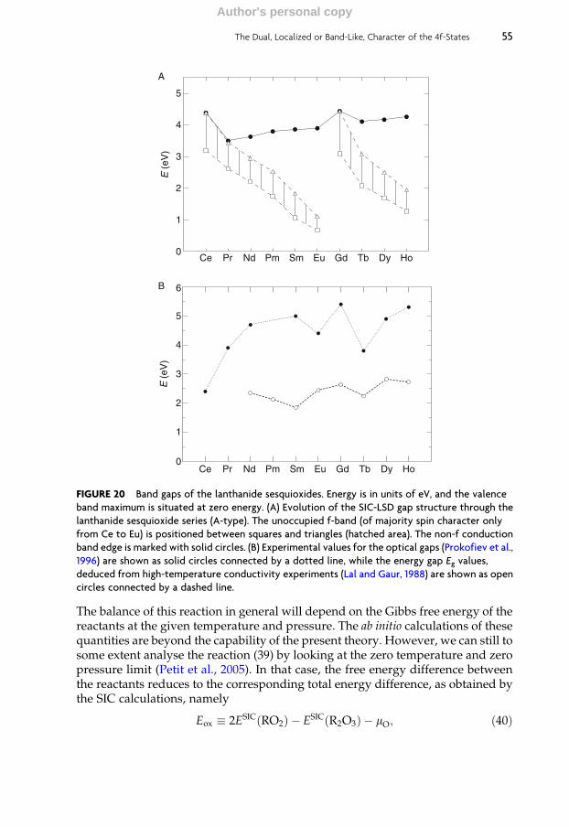
The balance of this reaction in general will depend on the Gibbs free energy of thereactants at the given temperature and pressure. The ab initio calculations of thesequantities are beyond the capability of the present theory. However, we can still tosome extent analyse the reaction (39) by looking at the zero temperature and zeropressure limit (Petit et al., 2005). In that case, the free energy difference betweenthe reactants reduces to the corresponding total energy difference, as obtained bythe SIC calculations, namely

Eox � 2ESIC RO2ð Þ � ESIC R2O3ð Þ � mO; ð40Þ

Ce Pr Nd Pm Sm Eu Gd Dy0

1

2

3

4

E (

eV)

5

6

Ce0

1

2

3

4

5

A

B

E (

eV)

HoDyTbGdEuSmPmNdPr

Tb Ho

FIGURE 20 Band gaps of the lanthanide sesquioxides. Energy is in units of eV, and the valence

band maximum is situated at zero energy. (A) Evolution of the SIC-LSD gap structure through the

lanthanide sesquioxide series (A-type). The unoccupied f-band (of majority spin character only

from Ce to Eu) is positioned between squares and triangles (hatched area). The non-f conduction

band edge is marked with solid circles. (B) Experimental values for the optical gaps (Prokofiev et al.,

1996) are shown as solid circles connected by a dotted line, while the energy gap Eg values,

deduced from high-temperature conductivity experiments (Lal and Gaur, 1988) are shown as open

circles connected by a dashed line.



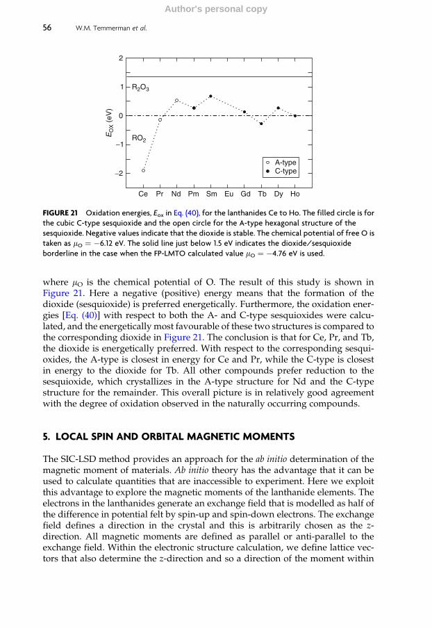
where mO is the chemical potential of O. The result of this study is shown inFigure 21. Here a negative (positive) energy means that the formation of thedioxide (sesquioxide) is preferred energetically. Furthermore, the oxidation ener-gies [Eq. (40)] with respect to both the A- and C-type sesquioxides were calcu-lated, and the energetically most favourable of these two structures is compared tothe corresponding dioxide in Figure 21. The conclusion is that for Ce, Pr, and Tb,the dioxide is energetically preferred. With respect to the corresponding sesqui-oxides, the A-type is closest in energy for Ce and Pr, while the C-type is closestin energy to the dioxide for Tb. All other compounds prefer reduction to thesesquioxide, which crystallizes in the A-type structure for Nd and the C-typestructure for the remainder. This overall picture is in relatively good agreementwith the degree of oxidation observed in the naturally occurring compounds.

5. LOCAL SPIN AND ORBITAL MAGNETIC MOMENTS

The SIC-LSD method provides an approach for the ab initio determination of themagnetic moment of materials. Ab initio theory has the advantage that it can beused to calculate quantities that are inaccessible to experiment. Here we exploitthis advantage to explore the magnetic moments of the lanthanide elements. Theelectrons in the lanthanides generate an exchange field that is modelled as half ofthe difference in potential felt by spin-up and spin-down electrons. The exchangefield defines a direction in the crystal and this is arbitrarily chosen as the z-direction. All magnetic moments are defined as parallel or anti-parallel to theexchange field. Within the electronic structure calculation, we define lattice vec-tors that also determine the z-direction and so a direction of the moment within

Ce

−2

−1

0

1

2

Pr Nd Pm Sm Eu Gd Dy

EO

X (

eV)

A-typeC-type

R2O3

RO2

HoTb

FIGURE 21 Oxidation energies, Eox in Eq. (40), for the lanthanides Ce to Ho. The filled circle is for

the cubic C-type sesquioxide and the open circle for the A-type hexagonal structure of the

sesquioxide. Negative values indicate that the dioxide is stable. The chemical potential of free O is

taken as mO ¼ �6.12 eV. The solid line just below 1.5 eV indicates the dioxide/sesquioxide

borderline in the case when the FP-LMTO calculated value mO ¼ �4.76 eV is used.



the crystal can be defined. The results discussed in this section are all the result offully self-consistent relativistic calculations unless otherwise stated. This is abso-lutely necessary for a quantitative evaluation of the orbital moments. We discussthe light lanthanides and the heavy lanthanides separately.

5.1 Hund’s rules

In the description of the standard model, Section 2.2, it is assumed that theelectrons distribute themselves among the available f-states according to Hund’srules. However, Hund’s rules are essentially based on experiment. A good first-principles theory of electronic structure is one where Hund’s rules drop out of thetheory rather than having to be included empirically.

As already said, to apply the SIC to the f-states, it is first necessary to decidewhich (and how many) states it should be applied to based on total energyconsiderations. Of course, it needs to be applied to the occupied states, but notto the unoccupied ones. If we take trivalent praseodymium as our example, thereare nominally two occupied f-states out of a possible 14, and in principle we canchoose to occupy any 2. Let us start by occupying two states of opposite spin and avariety of possible ml quantum numbers. During iteration to self-consistency, theSIC-states adjust but largely keep their initial characteristics, that is the schemepossesses many different solutions, which can be accessed by different startingconditions. In the end, it is the total energy that selects the proper ground state.For each arbitrarily chosen pair of initially occupied ml values, a fully self-consistent SIC-LSD calculation is performed and we plot the energy and thetotal orbital moment. This process is repeated choosing two states with parallelspins. The results of this are shown in Figure 22. It is clear that the data pointsseparate into two clusters. Those above –2.28 Ry are those where the two spins areanti-parallel (solid circles) and those below –2.28 Ry are those with parallel spins(open circles). Evidently lining up the spins parallel to each other of the individualstates is energetically preferable to having them anti-parallel, and so Hund’s firstrule is satisfied. Examining this figure further, we see that for the states withparallel spin, there is a rough linearity between the total energy and the orbitalmoment with the minimum total energy being when the orbital moment hasmaximum magnitude anti-parallel to the spin moment. Clearly, then Pr obeysall three of Hund’s rules. In all honesty, Pr is the best example, but the trendsdisplayed here are also observed in all the light lanthanides. In the heavy lantha-nides, similar behaviour is displayed but the lowest total energy is when theorbital moment is a maximum and parallel to the spin moment, also completelyconsistent with Hund’s rules.

5.2 The heavy lanthanides

Although the relativistic SIC-LSD (Beiden et al., 1997) calculations have beencarried out for all the lanthanide metals, we start discussing results from theheavy lanthanides. Thus, in Figures 23 and 24, we display the densities of statesfor Tb and Ho as illustrative examples. Figure 23A shows the majority spin d and f



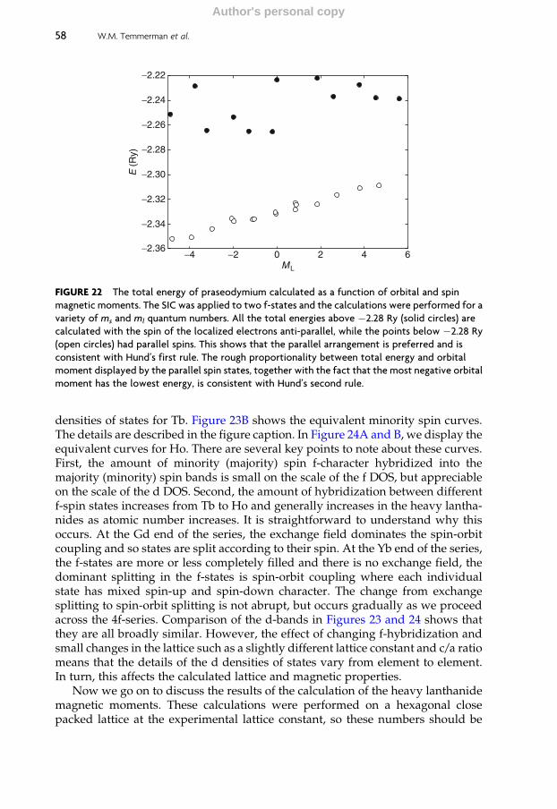
densities of states for Tb. Figure 23B shows the equivalent minority spin curves.The details are described in the figure caption. In Figure 24A and B, we display theequivalent curves for Ho. There are several key points to note about these curves.First, the amount of minority (majority) spin f-character hybridized into themajority (minority) spin bands is small on the scale of the f DOS, but appreciableon the scale of the d DOS. Second, the amount of hybridization between differentf-spin states increases from Tb to Ho and generally increases in the heavy lantha-nides as atomic number increases. It is straightforward to understand why thisoccurs. At the Gd end of the series, the exchange field dominates the spin-orbitcoupling and so states are split according to their spin. At the Yb end of the series,the f-states are more or less completely filled and there is no exchange field, thedominant splitting in the f-states is spin-orbit coupling where each individualstate has mixed spin-up and spin-down character. The change from exchangesplitting to spin-orbit splitting is not abrupt, but occurs gradually as we proceedacross the 4f-series. Comparison of the d-bands in Figures 23 and 24 shows thatthey are all broadly similar. However, the effect of changing f-hybridization andsmall changes in the lattice such as a slightly different lattice constant and c/a ratiomeans that the details of the d densities of states vary from element to element.In turn, this affects the calculated lattice and magnetic properties.

Now we go on to discuss the results of the calculation of the heavy lanthanidemagnetic moments. These calculations were performed on a hexagonal closepacked lattice at the experimental lattice constant, so these numbers should be

−4−2.36

−2.34

−2.32

−2.30

−2.28

−2.26

−2.24

−2.22

E (

Ry)

−2ML

20 64

FIGURE 22 The total energy of praseodymium calculated as a function of orbital and spin

magnetic moments. The SIC was applied to two f-states and the calculations were performed for a

variety of ms and ml quantum numbers. All the total energies above �2.28 Ry (solid circles) are

calculated with the spin of the localized electrons anti-parallel, while the points below �2.28 Ry

(open circles) had parallel spins. This shows that the parallel arrangement is preferred and is

consistent with Hund’s first rule. The rough proportionality between total energy and orbital

moment displayed by the parallel spin states, together with the fact that the most negative orbital

moment has the lowest energy, is consistent with Hund’s second rule.



−1.0E (Ry)

0−1.5E (Ry)

00

20

40

60

DO

S (

stat

es/R

y/ce

ll) 80

100A B

0.5−0.5−1.0 −0.5 0.5

FIGURE 23 The d (dashed lines) and f (full lines) densities of states for Tb with respect to the

Fermi energy. (A) Majority spin: the very tall and narrow peaks at around �1.15Ry are the majority

spin f-states. The small peak at �0.85 is majority spin f hybridized into the minority spin states

through spin-orbit coupling. From �0.25 to 0.5Ry, the d-bands dominate the DOS, but the lower

curve indicates a very small majority spin f-contribution in this region. (B) Minority spin: there is

considerable minority spin character hybridized into the occupied spin-up f-states. The single

occupied predominantly minority spin f-state is at�0.85Ry. The minority spin f-states are close to

the Fermi energy and these overlap and hybridize with the d-bands.

−1.0E (Ry)

0−1.5E (Ry)

00

20

40

60

DO

S (

stat

es/R

y/ce

ll) 80

100A B

0.5−0.5−1.0 −0.5 0.5

FIGURE 24 The d (dashed lines) and f (full lines) densities of states for Ho with respect to the

Fermi energy. (A) Majority spin: The very tall and narrow peaks at around �1.1Ry are the majority

spin f-states. The small peaks at �0.85 are majority spin f hybridized into the minority spin states

through spin-orbit coupling. From �0.25 to 0.5Ry, the d-bands dominate the DOS, but the lower

curve indicates a very small majority spin f-contribution in this region. There is considerable

majority spin DOS hybridized into the d-bands around the Fermi energy. (B) Minority spin: There is

considerable minority spin character hybridized into the occupied spin-up f-states. The three

occupied predominantly minority spin f-states are at�0.85Ry. The minority spin f-states are close

to the Fermi energy and these overlap and hybridize with the d-bands.



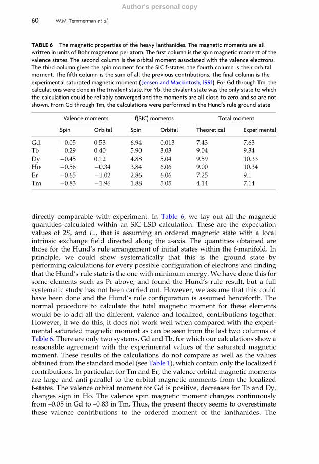
directly comparable with experiment. In Table 6, we lay out all the magneticquantities calculated within an SIC-LSD calculation. These are the expectationvalues of 2Sz and Lz, that is assuming an ordered magnetic state with a localintrinsic exchange field directed along the z-axis. The quantities obtained arethose for the Hund’s rule arrangement of initial states within the f-manifold. Inprinciple, we could show systematically that this is the ground state byperforming calculations for every possible configuration of electrons and findingthat the Hund’s rule state is the one with minimum energy. We have done this forsome elements such as Pr above, and found the Hund’s rule result, but a fullsystematic study has not been carried out. However, we assume that this couldhave been done and the Hund’s rule configuration is assumed henceforth. Thenormal procedure to calculate the total magnetic moment for these elementswould be to add all the different, valence and localized, contributions together.However, if we do this, it does not work well when compared with the experi-mental saturated magnetic moment as can be seen from the last two columns ofTable 6. There are only two systems, Gd and Tb, for which our calculations show areasonable agreement with the experimental values of the saturated magneticmoment. These results of the calculations do not compare as well as the valuesobtained from the standard model (see Table 1), which contain only the localized fcontributions. In particular, for Tm and Er, the valence orbital magnetic momentsare large and anti-parallel to the orbital magnetic moments from the localizedf-states. The valence orbital moment for Gd is positive, decreases for Tb and Dy,changes sign in Ho. The valence spin magnetic moment changes continuouslyfrom –0.05 in Gd to –0.83 in Tm. Thus, the present theory seems to overestimatethese valence contributions to the ordered moment of the lanthanides. The

TABLE 6 The magnetic properties of the heavy lanthanides. The magnetic moments are all

written in units of Bohr magnetons per atom. The first column is the spin magnetic moment of the

valence states. The second column is the orbital moment associated with the valence electrons.

The third column gives the spin moment for the SIC f-states, the fourth column is their orbital

moment. The fifth column is the sum of all the previous contributions. The final column is the

experimental saturated magnetic moment ( Jensen and Mackintosh, 1991). For Gd through Tm, the

calculations were done in the trivalent state. For Yb, the divalent state was the only state to which

the calculation could be reliably converged and the moments are all close to zero and so are not

shown. From Gd through Tm, the calculations were performed in the Hund’s rule ground state

Valence moments f(SIC) moments Total moment

Spin Orbital Spin Orbital Theoretical Experimental

Gd �0.05 0.53 6.94 0.013 7.43 7.63Tb �0.29 0.40 5.90 3.03 9.04 9.34Dy �0.45 0.12 4.88 5.04 9.59 10.33Ho �0.56 �0.34 3.84 6.06 9.00 10.34Er �0.65 �1.02 2.86 6.06 7.25 9.1Tm �0.83 �1.96 1.88 5.05 4.14 7.14



SIC-LSD method has a slight tendency to overlocalize states and as a result bringsa small amount of unphysical valence f-states below the Fermi energy. This meansthat the lanthanides become divalent slightly too early as we proceed across thePeriodic Table (Strange et al., 1999). The extra unphysical valence f-states replaced-states. However, they play a similar role in bonding to the d-states, so do notaffect the prediction of crystal structural properties, but can distort the predictionof the magnetic moment.

A better agreement with experiment is obtained if the valence moments areignored, as in the following procedure. The SIC states are highly localized ona particular lattice site. This can be seen from Table 6 where the values of Lz andSz of the SIC states of f-character are essentially the atomic values presentedin Table 1. Thus, we may interpret these as projections onto the z-axiscorresponding to effective S, L, and ensuing J quantum numbers, which can beused in Eqs. (4) and (5) to determine the total magnetic moment due to the SICstates. In this estimate, the moment of the occupied valence states is ignored. InTable 7, we show the results of this procedure and compare them directly withthe experimental values. Surprisingly with the omission of the spin and orbitalmoments of the valence states, we obtain excellent agreement between theoryand experiment. This can indicate that the experiment provides only the contri-bution of the localized states to the spin and orbital magnetic moments. This isplausible since these experimental magnetic moments are deduced from thelinear dependence of the inverse magnetic susceptibilities on temperature inthe high-temperature paramagnetic phases, Eq. (6). At these elevated tempera-tures, the magnetic behaviour is best described by the DLM model (see the nextsection), according to which the local f magnetic moments are not aligned butrather point randomly in all directions. As a consequence, one does not expectmuch of a valence electron polarization to develop and could even be negligible,which we assumed in our analysis presented in Table 7. The success of thisreasoning might also be construed as an illustration on how well the SICdescribes the localized part of the f-states.

TABLE 7 The magnetic properties of the heavy lanthanides. The magnetic moments are all

written in units of Bohr magnetons per atom. The first three columns are the S, L, and J quantum

numbers and gJ is the effective Lande g-factor, all of which can be compared with the equivalent

results in Table 1. The remaining columns are, respectively, the effective moments calculated

according to Eq. (5) and the experimental moment deduced from the Curie-Weiss behaviour of the

magnetic susceptibilities in the paramagnetic phases (Jensen and Mackintosh, 1991). The Hund’s

rule ground state was chosen throughout

S L J gJ mt me

Gd 3.47 0.013 3.48 1.997 7.88 7.95Tb 2.95 3.03 5.98 1.493 9.65 9.5Dy 2.44 5.04 7.48 1.326 10.56 10.6Ho 1.92 6.06 7.98 1.240 10.50 10.4Er 1.43 6.06 7.49 1.191 9.50 9.5Tm 0.94 5.05 5.99 1.157 7.49 7.3



5.3 The light lanthanides

In this section, we discuss some calculations of the magnetic moments of the lightlanthanides using SIC-LSD in a variety of situations. We have calculated themagnetic moments of all the light lanthanides on an fcc lattice with an identicalvolume per atom for each element. This has enabled us to untangle the effect ofsmall lattice constant changes on the moment from the effect of the extra f-electronas we proceed across the Periodic Table. The results of these calculations areshown in Tables 8 and 9, where we have explicitly shown all contributions tothe moment. In Table 8 are shown the ordered moments, whereas in Table 9 areshown the paramagnetic moments, extracted as outlined for the heavy lantha-nides in subsection 5.2.

TABLE 8 The magnetic properties of the light lanthanides. The magnetic moments are all written

in units of the Bohr magneton. The first column is the spin magnetic moment of the valence states.

The second column is the orbital moment associated with the valence electrons. Column three

is the spin moment for the SIC f-states, the next column is their orbital moment. The fifth

column is the total moment and the last column is the experimental saturated magnetic moment

(Jensen and Mackintosh, 1991). For Ce through Sm, the calculations were done in the trivalent

state, whereas for Eu, the calculation was done in the divalent state. From Ce through Sm, the

state chosen was the Hund’s rule ground state and this turned out to be the lowest energy state

Valence moments f(SIC) moments Total moment

Spin Orbital Spin Orbital Theoretical Experimental

Ce 0.32 0.03 0.96 2.96 1.71 0.6Pr 0.44 0.16 1.98 4.96 2.7 2.7Nd 0.34 0.51 2.94 5.93 3.16 2.2Pm 0.32 1.74 3.94 5.95 3.43 –Sm 0.55 1.69 4.94 4.94 1.14 0.13Eu 0.42 0.001 6.96 0.01 7.37 5.1

TABLE 9 The magnetic properties of the light lanthanides.The magnetic moments are all

written in units of Bohr magnetons per atom. The first three columns are the S, L, and J

quantum numbers and gJ is the effective Lande g-factor, all of which can be compared with

the equivalent results in Table 1. The remaining columns are the calculated effective moment

calculated according to Eq. (5) and the experimental moment (Jensen and Mackintosh, 1991).

The Hund’s rule ground state was chosen throughout

S L J gJ mt me

Ce 0.48 2.96 2.48 0.93 2.73 2.4Pr 0.99 4.96 3.97 0.80 3.55 3.5Nd 1.47 5.93 4.46 0.73 3.60 3.5Pm 1.97 5.95 3.98 0.60 2.67Sm 2.47 4.94 2.47 0.29 0.84 1.5Eu 3.48 0.01 3.47 1.96 7.72 3.4



It is notable that the spin and orbital contributions of the localized states arenearly the same as for the ionic case. This shows that in the light lanthanides, thef-states are as localized as for the heavy lanthanides. For the paramagneticmoments, the agreement between theory and experiment is very satisfactory(Table 9) and much better than using a band description of adding the contribu-tions of the localized and delocalized states (Table 8). Sm and Eu are less welldescribed by this procedure and it could be that the assumption of pure trivalentSm and pure divalent Eu are not fully applicable and some divalent Sm and sometrivalent Eu might be mixed into the ground state.

Now let us consider the effect of crystal environment on the magnetic momentof the lanthanides. In Table 10, we show the results of calculations of the magneticmoment of neodymium on several common crystal lattices. A trivalent Nd ionyields a spin moment of 3mB and an orbital moment of 6mB. In the final twocolumns of Table 10, we see that the SIC-LSD theory yields values slightly lessthan, but very close to, these numbers. This is independent of the crystal structure.The valence electron polarization varies markedly between different crystal struc-tures from 0.34mB on the fcc structure to 0.90mB on the simple cubic structure. It isnot at all surprising that the valence electron moments can differ so stronglybetween different crystal structures. The importance of symmetry in electronicstructure calculations cannot be overestimated. For example, the hcp lattice doesnot have a centre of inversion symmetry and this allows states with differentparity to hybridize, so direct f–d hybridization is allowed. However, symmetryconsiderations forbid f–d hybridization in the cubic structures. Such differences inthe way the valence electrons interact with the f-states will undoubtedly lead tostrong variations in the valence band moments.

6. SPECTROSCOPY

In this section, we highlight two spectroscopies that can reveal information on thevalence of the lanthanide ion. First, we will discuss high-energy photoemissionspectroscopy that shows the multiplet nature of the lanthanide ion. Second, we

TABLE 10 The magnetic properties of neodymium on a variety of crystal lattices (fcc, bcc, simple

cubic, and hexagonal lattices) calculated as described in the text. The magnetic moments are all

written in units of the Bohr magneton. The second column is the spin magnetic moment of the

valence s, p, d, and f-states. The third column is the orbital moment associated with the valence

electrons. The final two columns are the spin and orbital magnetic moments of the SI-corrected

f-states

Valence moments f(SIC) moments

Spin Orbital Spin Orbital

fcc 0.34 0.51 2.94 5.93bcc 0.75 0.51 2.95 5.95sic 0.90 0.88 2.93 5.89hcp 0.74 0.34 2.94 5.96



discuss resonant MXRS that allows us to study directly the spin and orbitalmagnetic properties of the late lanthanides. This experimental probe also hasthe potential to determine the number and symmetry of the localized f-states. Inthe first spectroscopy, the starting band structure is that of the LDA, while in thesecond one, the SIC-LSD is used.

6.1 Hubbard-I approach to lanthanide photoemission spectra

Photoemission is a powerful spectroscopy of lanthanide systems (Campagnaet al., 1979). This is due to the distinct atomic multiplet features, which serve asa fingerprint of the configuration adopted by the lanthanide ion in the solidenvironment.

In photoemission, a photon g of energy ho impinges on a solid, which is anN-electron system in its ground state |N; 0i. The photon is absorbed and itsenergy is transferred to an electron, which is emitted, leaving behind a solidwith only N�1 electrons and in some excited state. Schematically,

g þ N; 0 >!j jN � 1; i > þ e: ð41Þ

The energy of the electron, Ee, is measured and contains information about theexcitation energies in the N�1 electron system:

Ee ¼ ho þ E N; 0ð Þ � E N � 1; ið Þ: ð42Þ

In principle, all possible excitations contribute to the photoelectron spectrumand the proper quantum mechanical amplitude must be calculated. For thelanthanides, the atomic limit corresponds to the assumption that the photoelec-tron spectrum is dominated by those processes, where the photon hits a particularion and causes an excitation on that ion without disturbing the remainder of thecrystal. In the standard model, the lanthanide ion would initially be in its trivalentf n configuration with the Hund’s rule ground state multiplet (Table 1 in Section2.2), and would be transferred into some multiplet 2Sþ1LJ within configurationf n�1when the photon has been absorbed. The photoelectron energy would thus be

Ee ho þ Eion f n; 0ð Þ � Eion f n�1; 2Sþ1LJ� �

; ð43Þ

where Eion is the atomic energy. The amplitude for this to happen is proportionalto the product of two matrix elements:

A / hce eikr�

�

�

�ff i�h f n�1; 2Sþ1LJÞj f j f n; 0i; ð44Þ

where the first factor is the matrix element of the photon field between thewavefunction of the outgoing electron ce and the f electron wavefunction ff,whereas the second factor is the matrix element of the f destruction operatorf between the final and initial f multiplets.

In view of the strength of the Coulomb interaction, the atomic limit is certainly aquite idealized assumption. For example, in the real world, the kicked out electronstill has some distance to travel through the solid before leaving at the surface and



might scatter off other atoms or electrons on its way (secondary processes). Fur-thermore, the sea of conduction electrons might react to the presence of a hole inthe f-shell of the targeted ion, with some partial transfer of relaxation energy to thephotoelectron (screening). Finally, the photon might induce some further excita-tions of the conduction electrons (shake up effects), for example by excitingplasmon oscillations. For a complete understanding of photoemission, all suchprocesses must be considered, which is a formidable task. It so happens that theatomic limit is a good first approximation for many lanthanide systems, so we willdescribe in the following text its implementation within the DMFT framework(Lichtenstein and Katsnelson, 1998) and compare with experimental spectra.

The atomicmultiplet DMFTmethod is a generalization of theHubbard-I approx-imation (Hubbard, 1963, 1964a, 1964b) to a full f-manifold of 14 orbitals. The modeladopted for the isolated atom considers only these 14 degrees of freedom, and theirinteraction through the Coulomb force in the atomic Hamiltonian

Hat ¼ 1

2

X

mjf gUm1m2m3m4 f

{

m1f{

m2fm3

fm4þ x

X

i

l!i� s!i � m

X

m

fþm fm: ð45Þ

Here, index mj labels the f orbitals, and f{

m and fm are creation and annihilationoperators. The first term in Eq. (45) is the electron–electron interaction, with thematrix element

Um1m2m3m4¼ð ð

f�m1

rð Þf�m2

r0ð Þfm3r0ð Þfm4

rð Þr� r0j j d3rd3r0

¼X

‘

a‘ðm1m2m3m4ÞF‘;ð46Þ

where ’m(r) are the f-orbitals. The Coulomb integrals may be expressed in termsof vector coupling coefficients, a‘, and Slater integrals, F‘, with ‘ ¼ 0; 2; 4; 6(Lichtenstein and Katsnelson, 1998). The second and third terms in Eq. (45) arethe spin-orbit interaction, and a chemical potential term used to align with theFermi level of the solid [see, e.g., Lebegue et al. (2006a)].

The Hamiltonian, Hat, is solved by exact diagonalization in the space of allpossible Slater determinants for each of the f n configurations needed in thecalculation (typically for the ground state configuration with n electrons and forthe n � 1 configurations corresponding to excited states). The eigenvalues andeigenvectors, denoted respectively by En and nij , are obtained and the atomicGreen’s function Gat

mm0 calculated as:

Gatmm0ðoÞ ¼

X

lv

glnhljcmjnihnjc{m0 jlio þ El � Ev

; ð47Þ

where the weight factor gln ¼ dl,0 þ dn,0 specifies that one of the states in the summust be a ground state (T ¼ 0). More generally, in a thermal environment, gln isgiven by the appropriate Boltzmann weights (Lichtenstein and Katsnelson, 1998).

From Gat the atomic self-energy, Satmm0 , is finally extracted



Satmm0 oð Þ ¼ odmm0 � Gat

� ��1

mm0 oð Þ; ð48Þ

to be inserted in the DMFT Eq. (36) for the solid. We have used the LDA asreference system to obtain G0. The procedure outlined above describes the multi-plets of the 4f atom and combines in a unified framework the strong intra-shellcorrelation effects related to the 4f electrons and the weaker interaction between s,p, and d electrons. Adding Sat to the LDA Hamiltonian on the right-hand side ofEq. (36) shifts the f-weight from the narrow LDA bands into the energy positionscorresponding to multiplet excitation energies. The matrix elements in the numer-ator of Eq. (47) ensure that the proper transition amplitudes, according to atomicselection rules, enter the spectral function in Eq. (37). Not included in the descrip-tion based upon Eq. (37) are the matrix elements between the outgoing photoelec-tron and the orbital of the left-behind hole. These matrix elements will depend onthe angular character of the photo-hole. However, in the applications to bediscussed in the following, we will focus on the f-part of the spectral functiononly, and compare to photoemission spectra using photon energies chosen so as toenhance the f-contribution. Viewed as a DMFT implementation, the above proce-dure is particularly simple since the impurity is uncoupled from the bath [Gbath

does not enter in the model Eq. (45)].In Figures 25 and 26, we show the calculated spectral functions, respectively,

for SmAs and SmS using the above theory (Svane et al., 2005). The chemicalpotential of the reference ion is chosen such that the ground state is f 5(6H) fortrivalent Sm in SmAs and f 6(7F) for divalent Sm in SmS with an energy separationto the lowest n�1 excited levels [ f 4(5I) of 4.0 eV for SmAs and f 5(6H) of 0.8 eV forSmS, respectively], to coincide with the experimental values for these energies.The Slater integrals entering into the Coulomb matrix in Eq. (46) are almost

00

E (eV)6−6−12

2

4

65D 5G5F 5I 7F

s

p

5X

SmAs

A(E

) (s

tate

s/eV

/cel

l)

12

FIGURE 25 The calculated spectral function of trivalent Sm in SmAs at equilibrium volume,

with a ¼ 5.91 A. The full curve shows the f-contribution and the dashed curve the non-f

contribution. The energy is given relative to the Fermi level. The main lines are characterized

by their final state characteristics, either As s, p-bands, or as Sm f n�1 multiplet term.



equal for the two compounds, F‘ ¼ 23:9; 10:6; 6:5; and 4:6 eV, respectively, for‘ ¼ 0; 2; 4; 6 (evaluated with the f-radial wave at an energy given by the centreof gravity of the occupied f-partial DOS). However, for the direct Coulombparameter, F0�U, a screened value of F0 ¼ 7.1 eV was used instead of theunscreened value quoted above.

The SmAs spectral function in Figure 25 shows four distinct peaks between �5and �12 eV corresponding to the f 4(5L), L ¼ D, G, F, I, final states in the photo-emission process. These states agree well with the three-peak structure observedby Pollak et al. (1974) at binding energies of approximately�10.0 eV,�8.2 eV, and�6.0 eV (presuming that the 5F emission is too weak to lead to a resolvable peak).In the positive frequency range, one observes the 7F peak just above the Fermilevel whereas the f 6 final states of S ¼ 2 are situated further up in energy,however, now with a considerable spread due to the many allowed multiplets.The position of the corresponding levels in the reference atomic calculation aremarked in the figure.

The SmS spectral function is shown in Figure 26. The spectrum is now char-acterized by the low binding energy three-peak structure, which is also observedin several experiments (Campagna et al., 1974b; Pollak et al., 1974; Chainani et al.,2002; Ito et al., 2002), at binding energies�0.8 eV,�1.5 eV, and�4.0 eV, andwhichis attributed to the 6H, 6F, and 6P final states (Campagna et al., 1974b). The latterstate coincides with the sulphur p-band, as also found in the calculations. Theresults in Figure 26 agree well with those obtained by Lehner et al. (1998) by asimilar theoretical procedure.

The two spectra of SmAs and SmS demonstrate the distinctly different signa-tures of trivalent and divalent Sm ions in photoemission. Recent experiments(Chainani et al., 2002; Ito et al., 2002) show traces of Sm f 5 emission in SmS

00

E (eV)6−6−12

2

4

66P 6F6H 8S

s

p

6P,I,D,G,F,HSmS

A(E

) (s

tate

s/eV

/cel

l)

12

FIGURE 26 The calculated spectral function of divalent Sm in SmS (black phase, a ¼ 5.95 A).

The full curve shows the f-contribution and the dashed curve the non-f contribution. The energy

is given relative to the Fermi level. The main lines are characterized by their final state

characteristics, either as Sulphur s, p-bands or as Sm f n�1 multiplet term.



photoemission experiments, possibly also present in older works (Pollak et al.,1974). It is unclear whether this is due to small impurity concentrations or impliesa more complicated ground state for SmS than the ideal divalent state, which isnormally assumed and indeed also was found by the SIC-LSD calculations dis-cussed in Section 4.3.1. It is well known that doping of SmS can lead to theintermediate valence phase, characterized by photoemission spectra of both thehigh and low binding energy type (Campagna et al., 1974b; Pollak et al., 1974). Theunoccupied states of SmS have been monitored with bremsstrahlung inversespectroscopy (Oh and Allen, 1984). The spectra reveal two broad structures,approximately 4.5 and 9 eV above the Fermi level, which are in good agreementwith the positions in Figure 26 of the 8S and 6P, I, D, G, F, H features, respectively.

As an example of application of the atomic multiplet theory to the elementalmetals (Lebegue et al., 2006a, 2006b), we show in Figure 27 a comparison of thecalculated and measured spectra for terbium. The removal part of the spectrum atnegative energies, corresponding to f 8 ! f 7 transitions, reveals the exchangesplitting between the 8S and 6L (L ¼ G, H, I) peaks, which in band languagetranslates into the minority and majority spin bands. At positive energy, thespectrum is dominated by the strong peak at 3 eV with a shoulder towards higherenergy. There is a one to one correspondence between the observed and calculatedpeaks, although their relative intensities differ, which could be a matrix elementeffect. For the high-energy shoulder, there is a 1.5 eV discrepancy in position,which could be due to the neglect of the non-f electrons in the theory. Similarly,the smaller hump-like spectral intensity observed in experiment, in the region justbelow the Fermi level, could be a reflection of the normal valence electrons,

0−12

E (eV)0

10

20

30

40

50

60 6H5/2

6H15/2

6G5/2

6I5/2

8S7/2

Inte

nsity

(ar

b. u

nits

)

84−4−8

FIGURE 27 The calculated f-contribution to the spectral function of Tb in the hcp structure at

the equilibrium volume computed within the Hubbard-I method (dashed line) compared with

experiments (circles). Experimental data are X-ray photoemission and bremsstrahlung isochromat

spectroscopy from Lang et al. (1981). The Fermi level is at zero energy and the dominating atomic

final states are marked.



possibly with some small interaction effects with the f-manifold, which are nottreated by the present theory.

As a final example we show in Figure 28 a mixed valence spectrum of TmSe(Lebegue et al., 2005). TmSe is situated between the predominantly trivalent TmSand the divalent TmTe in the thulium monochalcogenides series. The figureshows data from two different experiments (Campagna et al., 1974a; Ufuktepeet al., 1998) with similar results, possibly with a relative shift in the Fermi levelposition. The recorded photoemission spectra exhibit both low lying excitations(between the Fermi level and 3 eV below) due to f 13 ! f 12 transitions and higherexcitations (between 5 and �13 eV below the Fermi level) due to f 12 ! f 11 transi-tions, each of these with their distinct multiplet structure. TmTe shows only theformer and TmS only the latter kinds of excitations (Lebegue et al., 2005). Again,there is good agreement between the positions of peaks in theory and experiment.The two experiments differ somewhat in the relative intensities of the divalentand trivalent parts. This could be an effect of different sample quality thatinfluences the relative balance of the f 13 and f 12 configurations in the mixed valentground state. A second possibility is a different surface sensitivity in the twoexperiments, combined with surface influence on the mixed valent ground state.

The theory presented here is not fully ab initio since it involves the adjustmentof the chemical potential as well as the F 0 (or Hubbard U) parameter. The Uparameter only enters in cases where three or more occupation numbers n of f n

configurations are involved, as is the case in the examples presented here. The sizeof multiplet splittings within a given configuration is solely determined by theF‘ ‘ > 0ð Þ parameters, which are calculated from the self consistent f partial wave,as the examples show with quite accurate results. Hence, screening effects do notenter as severely into the higher F‘ Slater integrals as they do for the Coulomb Uparameter.

0

10

0−4E (eV)

−8−12

20

30

Inte

nsity

(ar

b. u

nits

)

40

50

84

FIGURE 28 The calculated f-contribution to the spectral function of TmSe at equilibrium volume

computed within the Hubbard-I method (full line) compared with photoemission spectrum of

Campagna et al. (1974b) (solid squares) and of Ufuktepe et al. (1998) (solid circles) (vertically

displayed for clarity). The Fermi level is at zero energy.



6.2 Relativistic theory of resonant X-ray scattering

MXRS is a well-developed technique for probing the magnetic and electronicstructures of materials. The foundations of the theory of MXRS were laid downbyBlume (1985). He showed that this spectroscopy is intrinsically relativistic. Lateron Blume and Gibbs (1988) developed the theory further to show that the orbitaland spin contributions to the magnetic moment can be measured separately usingMXRS with a judicious choice of experimental geometry and polarization of theX-rays. This makes it a potentially very powerful spectroscopy. Integration of theSIC into the MXRS theory enables us to describe lanthanide and actinide materialson an equal footing with transition and simple materials. We then go further andmake the connection between this theory and the standard theories of resonantX-ray scattering (Hill and McMorrow, 1996; Lovesey and Collins, 1996) and illus-trate it with a calculation for the heavy lanthanides. In the relativistic SIC-LSDapproach (Beiden et al., 1997), we adopt the same strategy as in the non-relativistictheory, but instead of Eq. (23), we have to solve the Dirac equation of the form

ch

ia�r þ mc2 b� I4ð Þ þ Veff rð Þ þ mBbs�Beff rð Þ þ VSIC

g rð Þ� �

cg rð Þ ¼X

g0lg;g0cg0 rð Þ;

ð49Þ

where a and b are Dirac matrices, Beff is an effective magnetic field, s4 and I4 are4�4 spin operator and unit matrices, respectively, and lg;g0 is the Lagrange multi-pliers matrix. The SIC potential is given by

VSICg rð Þ ¼ � e2

4pe0

ð

ng r0ð Þr� r0j jd

3r0 þ dELSDxc �ng rð Þ�

dng rð Þ � mBbs4�dELSD

xc �ng rð Þ�

dmg rð Þ

� �

; ð50Þ

with g denoting orbitals and

mg rð Þ � �mBc{g rð Þbs4cg rð Þ:

The task of finding the single particle-like wavefunctions is now in principleequivalent to that within non-relativistic SIC-LSD theory. The four-componentnature of the wavefunctions and the fact that neither spin nor orbital angularmomentum are conserved separately presents some added technical difficulty,but this can be overcome using well-known techniques (Strange et al., 1984). Theformal first-principles theory of MXRS, for materials with translational periodic-ity, is based on the fully relativistic spin-polarized SIC-LSDmethod in conjunctionwith second-order time-dependent perturbation theory (Arola et al., 2004).

6.2.1 Basic theory of X-ray scatteringThe theory of X-ray scattering is based on the second-order golden rule for thetransition probability per unit time:

wif ¼2p

hh f jH0

intjiiþX

I

h f jH0intjIihIjH0

intjiiEi � EI

�

�

�

�

�

�

�

�

�

�

2

dðEf � EiÞ; ð51Þ



where jii; jIi; andj f i are the initial, intermediate, and final states of the electron–photon system. Ei, EI, and Ef are the corresponding energies. H0int is the time-independent part of the photon–electron interaction Hamiltonian

Hint tð Þ ¼ �e

ð

1c{r; tð Þac r; tð Þ�A r; tð Þd3r ð52Þ

where A r; tð Þ is the quantized radiation field operator, and c r; tð Þand c{r; tð Þ are

the quantized Dirac field operators. The formalism to reduce Eq. (51) to single-electron-like form has been published previously (Arola et al., 1997). Therefore,we will not repeat the details here, but only the equations that are key to anunderstanding of the theory.

In relativistic quantum theory, it is the second term in Eq. (51) that is entirelyresponsible for scattering as it is second order in the vector potential. It is conve-nient to divide this term into four components, and the X-ray scattering amplitudein the case of elastic scattering may be written as (Arola et al., 1997; Arola andStrange, 2001)

fql;q0l0ðoÞ ¼P

I;eL>0

h f jH0intjIihIjH0

intjiiEi � EI

�X

I;eL>0

h f jH0intjIihIjH0

intjiiEi � EI

¼ fþðposÞql;q0l0 ðoÞ þ f

�ðposÞql;q0l0 ðoÞ þ f

þðnegÞql;q0l0 ðoÞ þ f

�ðnegÞql;q0l0 ðoÞ;

ð53Þ

where q, l (q0, l0) represent the wave vector and polarization of the incident(outgoing) photon. Two different terms arise, as the distinction in energy ismade between eL > 0 and eL < 0 according to whether the intermediate statescontain excitations from the ‘negative-energy sea of electrons’, that is the creationof electron–positron pairs. For both positive and negative energies, there are twoseparate types of intermediate states, Iij , that is those containing no photons andthose containing two photons, which altogether results in the four separate scat-tering amplitudes. In the energy range of interest, ho << 2mc2, three of thesecomponents (the latter three) have no resonance, and so will only make a contri-bution to the cross section that is slowly varying. In the following, we shall only beinterested in scattering around resonance, and the corresponding expression forthe scattering amplitude reduces to the component that is large and rapidlyvarying around resonance, namely

fql;q0l0 oð Þ ¼ fþposql;q0l0 oð Þ ¼ �

X

LL0

Ð

d3r u{L rð ÞX{q0l0 rð ÞuL0 rð Þ

Ð

d3r0u{L

0 r0ð ÞXql r0ð ÞuL r0ð ÞeL � eL0 þ ho

ð54Þwhere uL (r) and uL (r) are positive and negative energy electron eigenstates withquantum numbers L of the Dirac Hamiltonian for the crystal and form a completeorthonormal set of four-component basis functions in the Dirac space. The one-electron states are subject to the constraint that eL � eF and eL0 > eF, where eF is theFermi energy. The relativistic photon–electron interaction vertex is

Xql rð Þ ¼ �ehc2

2Ve0o

� �1=2

a�e lð Þ qð Þeiq�r; ð55Þ



where e ¼ � ej j; and e lð Þ qð Þ is the polarization vector for the X-ray propagating inthe direction of q.

Equation (54) represents scattering with no photons and positive energy elec-trons only in the intermediate state. The corresponding theory is only applicablearound resonance that makes it complementary to the work of Blume (1985),which is only valid well away from resonance.

The final expression for the resonant part of the scattering amplitude in Braggdiffraction is

fþ posð Þql;q0l0

oð Þ ¼ fþ posð Þ0;ql;q0l0 oð ÞNcellsdQK; ð56AÞ

whereNcells stands for the number of unit cells,K is a reciprocal lattice vector,Q�q0– q, and the 0th unit cell contribution to the scattering amplitude is

fþ posð Þ0;ql;q0l0 oð Þ ¼

X

j

V

2pð Þ3ð

k21:BZd3k

X

Ntype

t¼1

X

Nt

i¼1

X

Lt

e�iQ�t tð Þi

�m

tið Þ þ jkLt

q0l0ð Þm tið Þ þ jk�

Ltqlð Þ

etð ÞLt

� ejk þ ho þ Gtð ÞLt=2

y ejk�eF� �

:

ð56BÞ

Here j is the band index, Ntype represents the number of different atom typesand Nt is the number of atoms of each type. The matrix elements m

tið Þ þ jkLt

qlð Þ aregiven by

mnð Þ þ jkLn

qlð Þ �ð

Snd3rnu

nð Þ{Ln

rnð ÞX{ql rnð Þcjk R 0ð Þ

n þrn

�

; ð56CÞ

where Sn refers to the nth atomic sphere within the unit cell. The added phenom-enological parameter G

tð ÞLt

represents the natural width of the intermediate statescreated by the core hole state Ltij at the t type basis atom.

Within the electric dipole approximation [eiq�r1 in Eq. (55)], the polarizationcan be taken outside the matrix elements and the scattering amplitude of Eq. (56B)can be written as

fþ posð Þ0;ql;q0l0

oð Þ ¼X

j

V

2pð Þ3ð

k21:BZd3kX

Ntype

t¼1

X

Nt

i¼1

X

Lt

e�iQ�t tð Þi

�l0�m tið Þ þ jk

Ltq0ð Þl�m tið Þ þ jk�

Ltqð Þ

etð ÞLt

� ejk þ ho þ Gtð ÞLt=2

y ejk�eF� �

;

ð57Þ

where the scalar product is between the photon polarization and the Pauli spinmatrices that appear within the matrix elements in this formulation. This equationcan be reduced to a rather appealing form. Using the notation

Qþ1 ¼1ffiffiffi

2p Qx þ iQy

� �

Q0 ¼ Qz Q�1 ¼1ffiffiffi

2p Qx � iQy

� �

ð58Þ



the numerator in Eq. (57) can be written as

l0�mðtiÞ þ jkLt

�

l�mðtiÞ þ jk�

Lt

�

¼X

n¼0;�1

l0

nln mðtiÞ þ jknLt

�

�

�

�

�

�

2

¼ 1

2l0�lð Þ m

tið Þ þ jkþ 1Lt

�

�

�

�

�

�

2 þ mtið Þ þ jk�1Lt

�

�

�

�

�

�

2 �h

þ imz� l0 � lð Þ mtið Þ þ jk�1Lt

�

�

�

�

�

�

2 � mtið Þ þ jk

þ1Lt

�

�

�

�

�

�

2 �

þ ðl0�mzÞðl�mzÞ

2 mðtiÞ þ jk0Lt

�

�

�

�

�

�

2

� mtið Þ þ jk

þ1Lt

�

�

�

�

�

�

2 � mtið Þ þ jk�1Lt

2�i

;�

�

�

�

�

�

ð59Þ

wheremz is a unit vector in the direction of the magnetization. The advantage of aformulation of the scattering amplitude in these terms is that the geometry of theexperiment is separated from the matrix elements and other atomic level informa-tion. It is possible to choose a geometry such that only one of the three terms inEq. (59) is non-zero. For example, if we have p–p scattering with 90 between theincident and outgoing beam, the first term is zero. If the magnetization points at90 to both the incident and outgoing polarizations, then the third term is zero andonly the second term remains. This cancellation was exploited in Brown et al.(2007) in the investigation of magnetism in lanthanide elements (see below).Furthermore, if a spherical approximation is made for the electronic structure,the matrix elements can be calculated as a function of energy just once and all theangular dependence of the scattering is in the polarization and mz dependence.

In the LMTO implementation, the resonant matrix element mtið Þ þ jkLt

qlð Þ can bewritten as

mtið Þ þ jkLt

qlð Þ ¼X

L

AjktiL u

tð ÞLtjX{

qljfntL

�

þ BjktiL u

tð ÞLtjX{

qljf�ntL

�h i

; ð60AÞ

where A and B are the wavefunction coefficients of the LMTO-ASA wavefunction(Skriver, 1983a) and ð f jX{

qljgÞ is defined as

fð jX{qljgÞ �

ð

Std3rf { rð ÞX{

ql rð Þg rð Þ; ð60BÞ

with f � uðtÞLt

and g � fntL or f�ntL

While the cross section is the fundamental measurable quantity in scatteringtheory, it is frequently more convenient in X-ray scattering from magnetic materi-als to measure the asymmetry ratio (dichroism). This is defined as the differencedivided by the sum of the cross section for the moment in one direction and themoment in the opposite direction.

A q;q0l;oð Þ � odO qþ;q0l0;oð Þ � odO q�;q0l0;oð ÞodO qþ;q0l0;oð Þ þ odO q�;q0l0;oð Þ ð61Þ

where the scattering rate odO into a solid space angle dO can be written in terms ofthe scattering amplitude fql;q0l0(o) as

odO ¼ 2p

hj fql;q0l0 oð Þj2 V

2pð Þ3o2

hc3dO ð62Þ



As shown by Lovesey and Collins (1996), the asymmetry ratio directly reflects thescattering amplitude rather than the cross section and emphasizes the interferencebetween magnetic scattering and charge scattering.

6.2.2 Application to lanthanidesAs discussed previously, the SIC-LSD method has been used successfully todescribe properties of lanthanide materials that cannot be described within thebare LDA (Strange et al., 1999). Here we look at how SIC-LSD describes resonantX-ray scattering. An important point made in the paper of Arola et al. (2004) is thatthe spectra are dependent on the number and symmetry of the localized states andintermediate states. Therefore, this spectroscopy could become quite importantfor the unravelling of the nature of the localized states.

Calculations of the asymmetry ratio for the heavy lanthanide metals have beencarried out by Brown et al. (2007). They have shown that the asymmetry ratioconsists of two features. There is a major peak in the asymmetry ratio that ispredominantly due to dipolar scattering from the magnetic moment of the 5dstates, and a smaller feature (below the elemental absorption edge) which in theirexperiment is also dipolar but in general is due to a mixture of dipolar andquadrupolar scattering. These features are labelled A and B, respectively, inFigure 29. Feature B remains more or less in the same place relative to theabsorption edge as we proceed along the lanthanide series whereas feature Agradually moves higher above the absorption edge. This means that these featuresseparate and feature B changes from being a shoulder on the side of feature A to aseparate peak. Note also the inversion of feature A in Tm. This is related to the factthat the d-electrons couple anti-ferromagnetically to the f-electrons in Tm, butferromagnetically in the other heavy lanthanides. Obviously the data in Figure 29are providing information about the details of the electronic structure of thelanthanides. In Figure 30, we present the 5d electron spin moment (left panel)and orbital moment (right panel) of the heavy lanthanides as a function of energy.As expected in the left panel, a lower energy peak is representing the majority spinstates and a higher peak is representing the minority spin states. Features A and Bfrom Figure 29 are also shown. It is clear that feature A in the scattering corre-sponds to the peak in the 5d minority spin states. Feature B does not correspondexactly to anything in the spin moment although it is fairly close in energy to themaximum in the majority spin moment as a function of energy. If we look at theright panel, the magnitude of the 5d orbital moment is generally small, althoughfor Er and Tm, it does become comparable to the spin moments. Clearly feature Ahas no correspondence with the orbital moment whereas feature B is close to apeak in the orbital moment. It is clear then that feature A arises from scatteringfrom the empty spin states anti-parallel to the f spin moments whereas feature Brepresents scattering from both the orbital and spin moments parallel to the f spinmoment. The correlation of peaks A and B in Figure 29, with the structure inFigure 30, demonstrates that the dipolar asymmetry ratios at the LIII edges reflectthe progression from spin-dominated Gd to orbital-dominated Er and Tm elec-tronic structure.



7. FINITE TEMPERATURE PHASE DIAGRAMS

7.1 Thermal fluctuations

Up to now, we have concentrated on the physics at zero kelvin. In this section, weextend the studies to finite temperatures and discuss finite temperature phasediagrams. The physics at finite temperatures is dominated by thermal fluctuationsbetween low lying excited states of the system. These fluctuations can include spinfluctuations, fluctuations between different valence states, or fluctuationsbetween different orbitally ordered states, if present. Such fluctuations can beaddressed through a so-called ‘alloy analogy’. If there is a timescale that is slowcompared to the motion of the valence electrons, and on which the configurationspersist between the system fluctuations, one can replace the temporal averageover all fluctuations by an ensemble average over all possible (spatially

0

AB

Gd

fpst, Mll cModel

Tb

Dy

Asy

mm

etry

rat

io (

arbi

trar

y un

its)

Ho

Er

Tm

E (eV)20−10 10

FIGURE 29 The asymmetry ratio of the lanthanides Gd through to Tm after Brown et al. (2007).

The circles represent the experimental results measured on the XMaS beamline at the ESRF. The

dashed line represents the full first-principles theory outlined in this section and yields at least

good qualitative agreement with experiment. The full line is a simple model calculation that

neglects all matrix elements and bases the asymmetry ratio on the DOS calculated using SIC-LSD

theory. Note the features A and B that are discussed in the text.



disordered) configurations of the system. In the following text, we will explainthis procedure in detail for the treatment of spin fluctuations, which leads to thewell-known DLM theory of finite temperature magnetism. After that, the samemethodology is applied to different valence configurations and demonstrated onthe example of the finite temperature phase diagram of Ce.

This static alloy analogy picture should be a good description as long as thereis a separation of timescales. If this breaks down, dynamical fluctuations—orquantum fluctuations—which are beyond this static picture, become important.These quantum fluctuations are the main emphasis of DMFT (Georges et al.,1996), which maps the system onto an effective Anderson impurity model,describing a dynamically fluctuating impurity in a self-consistently determinedeffective host. So far, DMFT has been formulated for model Hamiltonians, such asthe Hubbard model, and material-specific results have been achieved by con-structing these model Hamiltonians from realistic band structure calculations. In

−5

SP

IN M

OM

EN

T (

µ B/e

V)

OR

BIT

AL

MO

ME

NT

(µ B

/eV

)

−0.5

−0.4

−0.3

−0.2

−0.1

0

0.1

-0.5

−0.4

−0.3

−0.2

−0.1

0

0.1B BA A

Gd

Tb

Dy

Hox2

Erx4

Tmx8

E (eV)

0 5 10 −5 0 5 10 15

FIGURE 30 The spin and orbital moments associated with the 5d states in the heavy lanthanide

metals after Brown et al. (2007). (A) The spin moment. The arrows on the left-hand side represent

the coupling to the empty f-states above EF. The zero of energy on this scale is the Fermi energy.

Also shown are features A and B from Figure 29. (B) The orbital moment of the 5d states. As

expected, this quantity is generally small, although it becomes comparable with the spin moment

in Er and Tm. The dashed line represents the case when the f-states are filled according to Hund’s

rules and the full line when they are filled directly opposite to Hund’s rules.



the context of model Hamiltonians, it has been shown (Kakehashi, 2002) thatDMFT is equivalent to a dynamical CPA. Hence, the static CPA approach, pre-sented here, corresponds to the static limit of a, still to be developed, fully ab initioversion of DMFT. A discussion on how such a theory could be constructed isgiven in Section 8.

7.2 Spin fluctuations: DLM picture

For low temperatures, calculations of the characteristics of the free energy (groundstate energy) of a magnetic material are all based on an electronic band structurefor a given configuration, such as a fixed spin-polarization, for example a uniformspin-polarization for a ferromagnet and fixed sublattice spin polarizations for ananti-ferromagnet, a given valence state, or, if present, a given orbital order. Withincreasing temperature, fluctuations between those configurations are inducedthat eventually destroy the long-range order. These collective electron modesinteract as the temperature is raised and are dependent upon and affect theunderlying electronic structure. In this and the following sections, we concentrateon magnetic order and magnetic excitations through spin fluctuations. For manymaterials, the magnetic excitations can be modelled by associating local spin-polarization axes with all lattice sites and the orientations vary very slowly onthe timescale of the electronic motions (Moriya, 1981). These ‘local moment’degrees of freedom produce local magnetic fields on the lattice sites that affectthe electronic motions and are self-consistently maintained by them. By takingappropriate ensemble averages over the orientational configurations, the system’smagnetic properties can be determined. The DLM DFT-based theory has beendeveloped and used in this context to describe the onset and type of magneticorder ab initio in manymagnetic systems (Gyorffy et al., 1985; Staunton et al., 1985;Staunton and Gyorffy, 1992). Moreover, the recent inclusion of relativistic effectsinto DLM theory produces an ab initio description of the temperature dependenceof magnetic anisotropy of metallic ferromagnets, which agrees well with experi-mental results and deviates qualitatively from simple, widely used models(Staunton et al., 2004, 2006). It is the incorporation of the LSIC method fordescribing strongly correlated electrons into the DLM theory that we focus on inthis section and its application to the magnetic structure of Gd and other heavylanthanide systems. The standard model of lanthanide electronic structure gives agood qualitative description of the formation and magnitude of the magneticmoments. It has long been understood that these local moments, formed predom-inantly by the localized f-electrons, interact with each other by spin-polarizing thesea of conduction electrons in which they sit. The RKKY interaction is the simplestexample of this effect. As we will show, our DLM-LSIC theory gives a quantitativeab initio description of this physics.

In principle, the extension of electronic DFT to finite temperatures was carriedout by Mermin (1965) soon after the pioneering papers of Hohenberg, Kohn, andSham (Hohenberg and Kohn, 1964; Kohn and Sham, 1965). The single-particleentropy is included and the effective one-electron fields involveOxc, the exchange-correlation part of the Gibbs free energy functional of particle and magnetization



densities. Formally, this can be expressed in terms of spin-dependent pair corre-lation functions gl(s, s

0; r, r0), that is

Oxc n;m½ � ¼ e2

2

ð1

0

dl

ð

d3r

ð

d3r0X

s;s0

ns rð Þns0 r0ð Þr� r0j j gl s; s0; r; r0ð Þ ð63Þ

where ns(r) is the spin resolved charge density.It would seem logical then simply to make the finite temperature extension of

the LDA (or GGA) that is successfully exploited in applications on the groundstate of magnetic materials in conjunction with, say, the SIC, to deal with locali-zed states where appropriate. So, for example, Oxc n;m½ � is replaced byÐ

d3rn rð ÞO0xc n rð Þð Þ where O0

xc is the exchange-correlation part of the Gibbs freeenergy of a homogeneous electron gas. This assumption allows the thermallyaveraged magnetization, M, along with the spin splitting of the electronic struc-ture to decrease only by the excitation of particle-hole, ‘Stoner’ excitations acrossthe Fermi surface. However, it severely underestimates the effects of the thermallyinduced spin-wave excitations. For lanthanide materials, these orientational mag-netic fluctuations are entirely neglected, whereas in transitionmetal ferromagnets,the reliance on Stoner particle-hole excitations causes the calculated Curie tem-peratures to be typically an order of magnitude too high with no obvious mecha-nism for the Curie-Weiss behaviour of the uniform static paramagneticsusceptibility found for many metallic systems.

Evidently, part of the pair correlation function gl(s, s0; r, r0) should be related

by the fluctuation dissipation theorem to the magnetic susceptibilities harbouringinformation about spin waves. These spin fluctuations interact as temperature isincreased and so Oxc [n, m] should deviate significantly from the local approxi-mation with a consequent impact upon the form of the effective single electronstates. Indeed, accounts of modern electronic structure theory for magnetic sys-tems (Staunton, 1994; Kubler, 2000) have large sections devoted to work that isconcerned with the modelling of spin fluctuation effects while maintaining thespin-polarized single electron basis.

Most of this work is based on a rather simple, pervasive picture of fluctuating‘local moments’ that stems from the belief of a timescale separation of the elec-tronic degrees of freedom. A conduction electron (in a lanthanide material) travelsfrom site to site on a much faster timescale than that of the collective spin wavemotion. So the dominant thermal fluctuation of the magnetization that thestraightforward finite temperature extension of spin-polarized band theorymisses can be pictured quite simply as orientational fluctuations of ‘localmoments’. These entities are the magnetizations within each unit cell of theunderlying crystal lattice that are largely determined by the localized f-electronsin the lanthanides, while in itinerant electron transition metal magnets, they areset up by the collective behaviour of all the electrons. Their orientations persist ontimescales long compared to electronic ‘hopping’ times. At low temperatures,their long wavelength, slow spin wave dynamics can be directly extracted fromthe transverse part of the magnetic susceptibility. At higher temperatures, themore complex behaviour can be described with a classical treatment. The energy



is considered of the many interacting electron system constrained to have a setinhomogeneous magnetization profile. From atomic site to atomic site, the localmagnetic moments are oriented along prescribed directions, that is producing a‘local moment’ configuration. Averages over such orientational configurations aresubsequently taken to determine the equilibrium properties of the system. M cannow vanish as the disorder of the ‘local moments’ grows. There remains, however,the issue as to which fluctuations are the most important.

Formally DFT (Gyorffy et al., 1985) is used to specify the ‘generalized’ grandpotential, O nð Þ ef gð Þ, of an interacting electron system which is constrained in sucha way that the site by site spin polarization axes are configured according toef g ¼ e1; e2;...;eN

�

, where N is the number of sites (moments) in the system. The{e}, classical unit vectors, are thus the degrees of freedom describing the localmoment orientations and O nð Þ ef gð Þ is the ‘local moment’ Hamiltonian. (Withrelativistic effects such as spin-orbit coupling included, the temperature depen-dence of magnetic anisotropy can be described. This means that orientations of thelocal moments with respect to a specified direction n within the material arerelevant.)

One way forward from this point is to carry out calculations of O nð Þ ef gð Þ for aselection of configurations (‘spin’ spirals, two impurities in a ferromagnet, mag-netically ordered supercells, etc.) by making some assumptions about the mostdominant fluctuations. One then fits the set of O nð Þ ef gð Þ’s to a simple functionalform. Typically a classical Heisenberg model, O nð Þ ef gð Þ ¼ �1=2

P

ijJijei �ej is set upand various statistical mechanics methods (e.g., Monte Carlo) are used to producethe desired thermodynamic averages. Many useful studies have been carried outin this way but there is a risk that a bias is produced so that some of the physics ismissed. The spin-polarized electronic structures of the restricted set of con-strained systems are not guaranteed to generate magnetic correlations that areconsistent with the chosen sampling of the orientational configurations. In otherwords, the electronic and magnetic structures are not necessarily mutually con-sistent. In the following, we summarize the main points of our DLM theory whichavoids these problems. Full details can be found in references Gyorffy et al. (1985),Staunton et al. (1985), and Staunton and Gyorffy (1992) and relativistic extensionin references Staunton et al. (2004, 2006).

The DLM picture is implemented within a multiple-scattering formalism(KKR) (Korringa, 1947; Kohn and Rostoker, 1954; Stocks et al., 1978; Stocks andWinter, 1982; Johnson et al., 1986). Some applications include the description ofthe experimentally observed local exchange splitting and magnetic short-rangeorder in both ultrathin Fe films (Razee et al., 2002) and bulk Fe (Gyorffy et al., 1985;Staunton et al., 1985), the damped RKKY-like magnetic interactions in the compo-sitionally disordered CuMn ‘spin-glass’ alloys (Ling et al., 1994), and the onset ofmagnetic order in a range of alloys (Staunton et al., 1997; Crisan et al., 2002). Bycombining it with the LSIC (Luders et al., 2005) for strong electron correlationeffects, we have recently used it to account quantitatively for the magnetic order-ing in the heavy lanthanides (Hughes et al., 2007). This gives an ab initio account ofthe well-known picture of f-electron magnetic moments interacting via the con-duction electrons.



We consider a collinear magnetic systemmagnetized with reference to a singledirection n at a temperature T. (A non-collinear generalization can be made bymaking the notation more complicated.) The orientational probability distributionis denoted by P nð Þ ef gð Þ, and its average for a lattice site i,

heii ¼ð

. . .

ð

eiPnð Þ ef gð Þde1 . . .deN ¼ mn; ð64Þ

is aligned with the magnetization direction n. The canonical partition functionand the probability function are defined as Z nð Þ ¼

Ð

. . .Ð

e�bO nð Þ ef gð Þde1 . . .deN and

P nð Þ ef gð Þ ¼ e�bO nð Þ ef gð Þ=Z nð Þ, respectively. The thermodynamic free energy thatincludes the entropy associated with the orientational fluctuations as well as

creation of electron-hole pairs is given by F nð Þ ¼ �1=b ln Z nð Þ� �

. By choosing a

trial Hamiltonian function, Onð Þ0 ef gð Þ with

Znð Þ0 ¼

ð

. . .

ð

e�bOnð Þ0

ef gð Þde1 . . .deN; ð65Þ

Pnð Þ0 ef gð Þ ¼ e�bO

nð Þ0

ef gð Þ

Znð Þ0

; ð66Þ

and Fnð Þ0 ¼ �1=bðln Z

ðnÞ0 Þ, the Feynman-Peierls Inequality (Feynman, 1955) implies

an upper bound for the free energy, that is,

F nð Þ � Fnð Þ0 þ hO nð Þ � O

nð Þ0 i0; ð67Þ

where the average refers to the probability Pnð Þ0 ef gð Þ. By expanding O

nð Þ0 ef gð Þ as

Onð Þ0 ef gð Þ ¼

X

i

o1 nð Þi eið Þ þ 1

2

X

i 6¼j

o2 nð Þi;j ei; ej� �

þ . . . ; ð68Þ

the ‘best’ trial system is found to satisfy (Gyorffy et al., 1985; Staunton andGyorffy, 1992)

hO nð Þi0ei � hO nð Þi0 ¼ hO nð Þ0 i0ei � hO nð Þ

0 i0; ð69Þ

hO nð Þi0ei; ej � hO nð Þi0 ¼ hO nð Þ0 i0ei ;ej � hO nð Þ

0 i0; ð70Þ

and so on, where hieiorhiei ;ej denote restricted statistical averages with ei or both eiand ej kept fixed, respectively. (In the following, we shall omit the superscript0 from the averages.)

If we set Onð Þ0 ef gð Þ as a sum of mean field Weiss terms, namely

Onð Þ0 ef gð Þ ¼

X

i

h!inð Þ �ei; ð71Þ

where h!inð Þ ¼ h

nð Þi n with

hnð Þi ¼

ð

3

4pei�nð ÞhO nð Þieidei; ð72Þ



the probability distribution factorizes as

Pnð Þ0 eif gð Þ ¼

Y

i

Pnð Þi eið Þ ð73Þ

with

Pnð Þi eið Þ ¼

exp �b h!

nð Þi �ei

� �

Znð Þi

¼ bhnð Þi

4p sinhbhnð Þi

exp �b h!

nð Þi �ei

� �

: ð74Þ

The average alignment of the local moments, proportional to the magnetization, is

m! nð Þ

i ¼ð

eiPnð Þ

i eið Þdei ¼ mnð Þi n ð75Þ

and

mnð Þi ¼ � d ln Z

nð Þi

d bhnð Þi

� ¼ 1

bhnð Þi

� cothbhnð Þi ¼ L �bh

nð Þi

�

ð76Þ

follows, where L(x) is the Langevin function. Moreover, the free energy of thesystem is

F nð Þ ¼ hO nð Þi þ 1

b

X

i

ð

Pnð Þ

i eið ÞlnP nð Þi eið Þdei: ð77Þ

Another way of writing the Weiss field is (Gyorffy et al., 1985)

hnð Þi ¼ S

1; nð Þi ¼ @hO nð Þi

@mnð Þi

: ð78Þ

Using Eqs. (74) and (76), this is shown to be equivalent to solving the equationof state

@F nð Þ

@mnð Þi

¼ 0: ð79Þ

7.2.1 The role of the CPAThe averaging over local moment configurations is conveniently carried out usingCPA technology (Soven, 1967; Stocks et al., 1978; Stocks andWinter, 1982; Johnsonet al., 1986). The electronic charge density and also the magnetization density,which sets the magnitudes, mf g; of the local moments, are determined from anSCF-KKR-CPA (Stocks and Winter, 1982; Johnson et al., 1986) calculation. For agiven set of (self-consistent) potentials, electronic charge and local moment mag-nitudes, the orientations of the local moments are accounted for by the similaritytransformation of the single-site t-matrices (Messiah, 1965),

ti eið Þ ¼ R eið Þti zð ÞR eið Þþ ; ð80Þ



where for a given energy (not labelled explicitly), ti zð Þ stands for the t-matrix witheffective field pointing along the local z-axis (Strange et al., 1984) and R eið Þ is aunitary representation of the O(3) transformation that rotates the z axis along ei.

The CPA determines an effective medium through which the motion of anelectron mimics the motion of an electron on the average. In a system magnetizedwith reference to a direction n, the medium is specified by t-matrices, t

nð Þi;c ,

which satisfy the condition (Stocks et al., 1978),

ht nð Þii ef gð Þi ¼

ð

ht nð Þii ieiP

nð Þi eið Þdei ¼ t

nð Þii;c ; ð81Þ

where the site-diagonal matrices of the multiple scattering path operator (Gyorffyand Stott, 1973) are defined as,

ht nð Þii iei ¼ t

nð Þii;cD

nð Þi eið Þ; ð82Þ

with the CPA projector

Dnð Þi eið Þ ¼ 1 þ ti eið Þð Þ�1 � t

nð Þi;c

��1� �

tnð Þii;c

� ��1

; ð83Þ

and

t nð Þc

¼ ððt nð ÞcÞ�1 � G

0Þ�1: ð84Þ

Equation (81) can be rewritten in terms of the excess scattering matrices,

Xnð Þi eið Þ ¼ t

nð Þi;c

��1� ti eið Þð Þ�1

� ��1

� tnð Þii;c

!�1

; ð85Þ

in the formð

Xnð Þi eið ÞP nð Þ

i eið Þdei ¼ 0: ð86Þ

Thus, for a given set of Weiss fields, hnð Þi , and corresponding probabilities,

Pnð Þi eið Þ; Eq.(86) can be solved by iterating together with Eqs. (85) and (84) to obtain

the matrices, tnð Þi;c (Staunton et al., 2006).

Using the magnetic force theorem, the single-particle energy part of the DFTgrand potential gives

O nð Þ ef gð Þ ’ �ð

de fb e; n nð Þ �

N nð Þ e; ef gð Þ; ð87Þ

as an effective ‘local moment’ Hamiltonian, where n nð Þ is the chemical potential,fb e; n nð Þ� �

is the Fermi-Dirac distribution, and N nð Þ e; ef gð Þ denotes the integratedDOS for the orientational configuration, {e}. From the Lloyd formula (Lloyd andBest, 1975),

N nð Þ e; ef gð Þ ¼ No eð Þ � 1

pIm ln det t nð Þ e; ef gð Þ�1 � G

0eð Þ

�

; ð88Þ



[N0(e) being the integrated DOS of the free particles] and properties of the CPAeffective medium, the partially averaged electronic Grand Potential is given by

hO nð Þiei¼ �ð


N nð Þc eð Þ

þ 1

p

ð


Im ln detMnð Þi e; eið Þ

þX

j6¼i

1

p

ð


Imhln detMnð Þj e; ej� �

i;

ð89Þ

and the Weiss field, hnð Þi , can be expressed, using Eq. (72), as

hnð Þi ¼ 3

4p

ð

ei�nð Þð

de fb e; n nð Þ � 1

pIm ln detM

nð Þi e; eið Þ

� �

dei; ð90Þ

where

Mnð Þi e; eið Þ ¼ 1 þ ti eið Þð Þ�1 � t

nð Þi;c

��1� �

tnð Þii;c

� �

and

Nnð Þc eð Þ ¼ � 1

pIm ln det t nð Þ

ceð Þ�1 �G

0eð Þ

�

:

The solution of Eqs. (90) and (76) produces the variation of the magnetization mnð Þi

with temperature T with mnð Þi going to zero at T ¼ T

nð Þc :

7.2.2 The paramagnetic DLM stateThe paramagnetic state is given by the Weiss fields being zero so that the prob-abilities, P

nð Þi ¼ 1=4p, and on any site, a moment has an equal chance of pointing in

any direction. This means the magnetizations, mnð Þi , vanish. The magnetic transi-

tion temperature, onset, and type of magnetic order can be extracted by studyingthe effects of a small inhomogeneous magnetic field on this high T paramagneticstate (Gyorffy et al., 1985; Staunton et al., 1985; Staunton and Gyorffy, 1992).

When relativistic spin-orbit coupling effects are omitted, the single-site matrix~t(ei) describing the scattering from a site with local moment orientated in thedirection ei becomes

~ti ¼1

2tþ þ t�ð Þ~1 þ 1

2tþ � t�ð Þ~s � ei; ð91Þ

where ~sx; ~sy; and ~sz are the three Pauli spin matrices defined according to theglobal z-axis. In the local reference frame, where the z-axis is aligned with ei, weevaluate the matrices tþ/t�, representing the scattering of an electron with spinparallel/anti-parallel to the local moment direction ei. These matrices are calcu-lated according to

tþ �ð ÞL eð Þ ¼ � 1ffiffi

ep sindþ �ð ÞL eð Þeidþ �ð ÞL eð Þ ð92Þ



where the phase shifts dL(e) are computed using effective DFT potentials. Theseeffective potentials, uþ and u�, differ on account of the ‘local exchange splitting’,which is the cause of the local moment formation. Unlike the conventional LSDAimplementation, the potentials uþ/u� are orbital dependent when the DLM theoryis combined with the SIC-LSD approach. This dependency comes about by ourSI-correcting certain L channels as discussed earlier. Importantly, the SI-correctedchannels of uþ and u� may differ. Indeed, as described in Section 3.6, the channelsto which we apply the SIC are those with a resonant phase shift (Luders et al.,2005). Such resonant behaviour is characteristic of well-localized electron states,which will establish quasi-atomic like moments. Through the influence they exerton the electron motions, these moments will be reinforced by the spins of moreitinerant-like electrons. It thus follows that resonant states will tend to define thelocal moment orientation and, as such, we expect to SI-correct a greater number ofchannels of uþ than we do for u�. For example, for Gd, all 7 uþ f-channels areSI-corrected while no correction is applied to any of the u� f-channels.

In the paramagnetic regime, we find

~D0

i ¼1

2D0

þ þ D0�

� �

~1 þ 1

2D0

þ �D0�

� �

~s � ei ð93Þ

where

D0þ �ð Þ ¼ 1 þ t�1

þ �ð Þ � tcð Þ�1h i

tc;00��1:

�

ð94Þ

The superscript 0 signifies that the CPA projector is evaluated in the paramagneticstate. Substituting Pi eið Þ ¼ P0 ¼ 1=4p into Eq. (81), we obtain

1

4p

ð

dei ~D0

i eið Þ ¼ ~1; ð95Þ

which becomes, on carrying out the integration,

1

2D0

þ þ 1

2D0

� ¼ 1: ð96Þ

Equation (96) is evidently just the CPA equation for a systemwith 50% ofmomentspointing ‘up’ and 50% pointing ‘down’, that is an Ising-like system. The electronicstructure problem is thus reduced to that of an equiatomic binary alloy, where thetwo ‘alloy’ components have anti-parallel local moments. Treating this ‘alloy’problem with the KKR-CPA, in conjunction with the LSIC charge self-consistencyprocedure, outlined in Section 3.6 and by Luders et al. (2005), we arrive at a fullyself-consistent LSIC-CPA description of the DLM paramagnetic state.

It should be noted that the equivalence of the DLM electronic structure prob-lem to that of an Ising-like system is purely a consequence of the symmetry of theparamagnetic state, and is not the result of our imposing any restriction on themoment directions. Indeed, in the formalism for the paramagnetic spin suscepti-bility, which we outline now, we maintain and consider the full 3D orientationalfreedom of the moments.



Within the DLM method, the magnetization at a site i, Mi, is givenby

Ð

dei mPi eið Þei; where m is the local moment magnitude, determined self-consistently. In the paramagnetic regime, where Pi is independent of ei andMi ¼ 0, we can study the onset of magnetic order by considering the response tothe application of an external, site-dependent magnetic field. Focusing on thedominant response of the system to line up the moments with the applied field,from the equation of state, we obtain the following expression for the static spinsusceptibility:

wij ¼b

3

X

k

Sð2Þik wkj þ

b

3dij; ð97Þ

where S(2) is the direct correlation function for the local moments, defined by

S2ð Þik ¼ � @2hOi

@mi@mk; ð98Þ

and depends only on the vector difference between the positions of sites i and k. Alattice Fourier transform can hence be taken of Eq. (97), giving

w qð Þ ¼ 1

3bm2 1� 1

3bS 2ð Þ qð Þ

� ��1

: ð99Þ

By investigating the wave vector dependence of the susceptibility, we gain infor-mation about the wave vector (q) dependence of the spin fluctuations that char-acterize the paramagnetic state and the type of magnetic order that might occur asthe temperature is lowered through a phase transition. For example in a ferro-magnetic material, such as gadolinium, the paramagnetic state is characterized byferromagnetic spin fluctuations, which have longwavelengths, q�(0, 0, 0), becom-ing unstable to them at the Curie temperature, TC. For a system that orders into anincommensurate anti-ferromagnetic structure, the paramagnetic state is domi-nated by ‘anti-ferromagnetic’ spin fluctuations, specified by a finite, incommen-surate, wave vector q ¼ Q0 which also characterizes the static magnetization orspin density wave state formed below the Neel temperature, TN. For example, themagnetic structures of the heavy lanthanides terbium (Tb) to thulium (Tm) aredescribed by wave vectors of the form Q0 ¼ (0, 0, qinc), where individual hexago-nal layers are uniformly magnetized in a direction that changes from layer to layeraccording to the modulation vector qinc.

An expression for S(2)(q), involving scattering quantities obtained from theelectronic structure of the paramagnetic state, can be found in Staunton et al.(1986). In brief:

S 2ð Þ qð Þ ¼ð

de fb e; v nð Þ � 1

pIm TrL0w

0qð ÞL qð Þ; ð100Þ

where

w0qð Þ ¼

ð

BZ

d3k tc kð Þtc k þ qð Þ � tc;00tc;00; ð101Þ



which is the lattice Fourier transform of the ‘non-interacting’ susceptibility for thesystem, and L qð Þ satisfies the following Dyson-like equation:

L qð Þ ¼ L0 þ L0w0qð ÞL qð Þ; ð102Þ

with L0 ¼ D0þ t�1

þ � t�1�

� �

D0�:

7.2.3 Magnetic order in gadolinium: The prototypeA summary of this work is provided by Hughes et al., (2007). Gadolinium’s hcpcrystal structure is parametrized by two variables, the c/a ratio of the latticeparameters and the atomic unit cell volume, expressed in terms of the WS radius.Experimentally, these two parameters are 1.597 and 3.762 a.u., respectively(Banister et al., 1954). A LSDA calculation of the DOS of gadolinium in itsparamagnetic (DLM) state at these lattice parameters reveals theminority 4f-statesmaking a significant contribution at the Fermi energy. This has important impli-cations for the magnetic ordering in the system (Heinemann and Temmerman,1994). A SIC-LSDA calculation, however, where all seven majority 4f-states arecorrected, opens up a Hubbard gap between the occupied and unoccupied f-states. The majority f-states are pushed down to approximately 16 eV below theFermi energy and the minority f-states are moved away from the conductionbands, reducing the f contribution to the DOS at the Fermi energy. The SIC-LSDA electronic structure thus describes the experimental picture well, with thef-states playing little role in conduction.

Figure 31 shows paramagnetic spin susceptibilities for gadolinium, cor-responding to these electronic structures. For the LDA calculation (a), the suscep-tibility attains its maximum at q ¼ (0,0,1), indicating that the system should orderwith a commensurate type 1 anti-ferromagnetic (AF1) structure, where magneticmoments are oppositely aligned in alternate planes along the c-axis. This isconsistent with ground state energy (T¼ 0 K) calculations from other LDA studiesof gadolinium (Heinemann and Temmerman, 1994), where an anti-ferromagneticstructure was found to be energetically favourable over the experimentallyobserved ferromagnetic structure. The origin of this AF1 coupling derives fromthe proximity of 4f minority states to the Fermi energy (Kurz et al., 2002). Previousinvestigations have shown that by pushing the 4f-states away from the Fermienergy, either by treating them as part of the core (Eriksson et al., 1995) orincluding a Coulomb parameter U for the f-states (LDA þ U) (Harmon et al.,1995), a ferromagnetic ground state can be obtained. Since the SIC succeeds inpushing the f-states away from the Fermi energy, the paramagnetic DLM stateshould show an instability to ferromagnetic order when the LSIC is included. Thisfeature is evident in Figure 31B, which shows the susceptibility attaining itsmaximum value at q ¼ 0. Note, however, the presence of a shoulder in thesusceptibility along the [001] direction, around q ¼ 0.2. This feature is significantas we shall show.

Having demonstrated that the LSIC gives an appropriate treatment of the 4f-states, leading to a ferromagnetic ground state, we proceed further with theinvestigation of gadolinium. We determined the theoretical lattice parameters of



the paramagnetic state from calculations of the total energy. The energy is mini-mized at a WS radius which is almost invariant of the c/a values. The overallminimum occurs at a c/a ratio of 1.63 and a WS radius of 3.654 a.u. We find theparamagnetic spin susceptibility for these lattice parameters to attain its maxi-mum at q ¼ 0 also and hence to infer ferromagnetic ordering.

Figure 32 shows the temperature dependence of the q ¼ 0 (ferromagnetic)susceptibility of gadolinium. A Curie-Weiss type behaviour is observed, withTC ¼ 280 K/324 K for the theoretical/experimental lattice parameters in fairagreement with that measured experimentally, TC ¼ 293 K ( Jensen andMackintosh, 1991). The effective magnetic moment was 7.34mB/7.36mB for thetheoretical/experimental lattice parameters, also in reasonable agreement withthe experimental value of 7.63mB and also the results from calculations where the4f-states were treated as part of the core [7.44mB (Turek et al., 2003)] or the LDAþUwas used [7.41mB (Kurz et al., 2002)]. Examining the l-decomposed spin densitiesobtained from the LSIC DOS shows the magnetic moment to originate mainly fromthe f-states (�6.95mB), with the remainder coming from a polarization of the d-states(�0.34mB) and a small contribution from the s- and p-states (�0.07mB).

In our computations, we find the magnetic ordering tendencies of gadoliniumto change as the lattice parameters are altered away from their equilibrium values.On changing the c/a ratio over the range 1.54–1.66, with theWS-radius fixed at the

0 0.2 0.4 0.6 0.8 1.0

15

10

5

0

20

q {0,0,1}

1.2

1.6

2.0

2.4

A

B

c(q

) [m

B2 /

mR

y]

FIGURE 31 Paramagnetic spin susceptibilities for gadolinium at wave vectors along the [0,0,1]

direction, obtained from (A) LSDA calculation and (B) LSIC-LSDA calculation.



theoretical value (3.654 a.u.), our calculated paramagnetic spin susceptibility,shown in Figure 33, starts to develop a shoulder near q ¼ (0,0,0.2), similar tothat observed in Figure 31B. Moreover, at the lowest c/a ratios, this shouldergrows into a peak and the susceptibility no longer attains its maximum value atq ¼ 0. The maximum occurs instead at some incommensurate wave vector, qinc,meaning that the system now has a tendency to order into an incommensuratemagnetic structure at low temperatures. This could be helical, where the helix turnangle, that is the angle between magnetic moments in adjacent layers, would begiven by pqinc.

Such incommensurate ordering is characteristic of the heavy lanthanide ele-ments, terbium to thulium, and is associated with a ‘webbing’ feature of their

0.0200

Tc = 280 K Tc = 324 K

Exp.Tc = 293 K

400

c−1 (

q=

0)

[(m

B2 /

mR

y)−1 ]

600

T (K)

0.4

0.8

1.2

Theoretical lattice parameters

Experimental lattice parameters

FIGURE 32 Inverse spin susceptibilities for Gd as a function of temperature, calculated for the

theoretical and experimental lattice parameters.

... . . . . . . . . . . . . . . ..

..

. .

... . . . . . . . . . . . . . . ..

..

.

... . . . . . . . . . . . . . . ..

. . .

... . . . . . . . . . . . . . . . . . .

... .. . . . . . . . . . . . . . . . .

..................................................................

0.40.0

0.0 0.2 0.4 0.6 0.8 1.0

0.1 0.2 0.3

0.6

0.8

1.0

c/a ratio1.541.571.5971.631.66

1.0

0.8

0.6

0.4

c(q

)/c(0

)

q {0,0,1}

FIGURE 33 Normalized paramagnetic spin susceptibilities for Gd, obtained using the theoretical

unit cell volume. The inset shows the susceptibility up to the zone boundary for c/a ratio 1.54.



Fermi surfaces. This webbing structure contains large parallel sheets of Fermisurface, which can nest together when translated by some vector in k-space. Thiscan cause an enhancement of the magnetic susceptibility at the nesting vector, andindeed it has been shown, both theoretically (Keeton and Loucks, 1968) andexperimentally (Dugdale et al., 1997), that the size of the nesting vector in theheavy lanthanides is correlated with their magnetic ordering vectors. The shape ofthe Fermi surface in heavy lanthanide metals depends critically on the c/a ratio ofthe lattice parameters (Cracknell and Wong, 1973), implying that the magneticstructures of these elements are sensitive to the c/a ratio. This is corroborated byexperimental studies by Andrianov and others, which have shown that it ispossible to alter the magnetic state of lanthanide metals and alloys by changingthe lattice parameters through application of external pressure or tension(Andrianov and Chistiakov, 1997; Andrianov et al., 2000) and by alloying withyttrium (Andrianov, 1995). Such behaviour is possibly interpreted in terms of anelectronic topological transition (Lifshitz, 1960; Blanter et al., 1994) at some criticalc/a ratio, where the webbing structure of the Fermi surface ruptures.

To analyse our susceptibility results shown in Figures 31B and 33, we investi-gate the Fermi surface of paramagnetic (DLM) gadolinium at various c/a ratios.For a given configuration of local moments, this Fermi surface can be defined inthe usual way. However, when considering the whole ensemble of momentorientations, the ‘Fermi surface’ is a smeared out average of itself over all momentconfigurations. A useful tool for defining this surface is the BSF (Faulkner, 1982)that is periodic in reciprocal wave vector k space and is given by

AB k;Eð Þ ¼ � 1

pImX

nm

exp½ik� Rn � Rmð Þ�ð

d3rhG r þ Rn; r þ Rm;Eð Þi; ð103Þ

in terms of an ensemble average, hi, of the electronic real space Green’s functionand where the integral over r is within the unit cell at the origin. In this case, theensemble average is taken over local moment configurations (Szotek et al., 1984).For ordered systems, AB(k, E) consists of a set of d-function peaks:

AB k;Eð Þ ¼X

n

d E� En kð Þð Þ; ð104Þ

where En(k) is the Bloch energy eigenvalue for the wave vector k and band indexn. With disorder (here the local moment spin fluctuation disorder), these peaksbroaden but their positions can be regarded as an effective band structure, withtheir width in energy interpreted as an inverse lifetime (Szotek et al., 1984). TheFermi surface of a disordered system is defined as the locus of these peaks at theconstant energy E ¼ EF.

Figure 34 shows the BSF of paramagnetic Gd at the Fermi energy, EF, calcu-lated for the sets of lattice parameters used in Figure 33. For c/a ratios of 1.597 orsmaller, a webbing feature is displayed and the corresponding nesting vector isindicated by an arrow in panel (a). At a c/a ratio of 1.63 (Figure 33D), the webbingfeature has started to rupture, and at a c/a ratio of 1.66 (Figure 33E), the rupturingis complete and the Fermi surface no longer has any significant regions of nesting.



This concurs with the results shown in Figure 33, where the susceptibility isenhanced at some incommensurate q vector for low c/a ratios, Figure 35Ashows a cross section through the webbing structure for c/a ratio 1.54. The nestingstructure is created by two bands which just cross the Fermi energy along the L–Mdirection. The broadening of the spectral function peaks, caused by the localmoment disorder, means that the bands are smeared, which results in theirmerging together at the L point. The magnitude of the nesting vector, Q0, is�0.2 (in units of 2p/c) and coincides with the size of the magnetic ordering wavevector, qinc, observed in Figure 33A. Figure 35B and C show the same cross sectionof the BZ, with the BSF evaluated using c/a ratios 1.57 and 1.66, respectively. Inpanel (b), the Fermi surface has a distinctive ‘dog-bone’ shape, with two extremalvectors, one centred and the other non-centred, connecting the sheets of Fermisurface. Figure 35A and B show the length of the centred nesting vector todecrease as the c/a ratio increases. This is in keeping with the experimental resultsof Andrianov, where the length of the magnetic ordering vector decreases contin-uously as the c/a ratio is increased. This does not, however, interpret the

A B

E

DC

FIGURE 34 Bloch spectral function of Gd in the hexagonal BZ, calculated at the Fermi energy.

Panels (A), (B), (C), (D), and (E) are for c/a ratios 1.54, 1.57, 1.597, 1.63, and 1.66, respectively,

with theoretical unit cell volumes used but not for high c/a ratios.



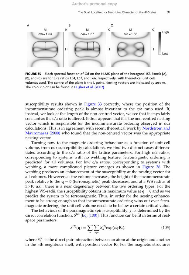
susceptibility results shown in Figure 33 correctly, where the position of theincommensurate ordering peak is almost invariant to the c/a ratio used. If,instead, we look at the length of the non-centred vector, we see that it stays fairlyconstant as the c/a ratio is altered. It thus appears that it is the non-centred nestingvector which is responsible for the incommensurate ordering observed in ourcalculations. This is in agreement with recent theoretical work by Nordstrom andMavromaras (2000) who found that the non-centred vector was the appropriatenesting vector.

Turning now to the magnetic ordering behaviour as a function of unit cellvolume, from our susceptibility calculations, we find two distinct cases differen-tiated according to the c/a ratio of the lattice parameters. For high c/a ratios,corresponding to systems with no webbing feature, ferromagnetic ordering ispredicted for all volumes. For low c/a ratios, corresponding to systems withwebbing, a more complicated picture emerges as shown in Figure 36. Thewebbing produces an enhancement of the susceptibility at the nesting vector forall volumes. However, as the volume increases, the height of the incommensuratepeak relative to the q ¼ 0 (ferromagnetic) peak decreases, and at a WS radius of3.710 a.u., there is a near degeneracy between the two ordering types. For thehighest WS-radii, the susceptibility obtains its maximum value at q ¼ 0 and so wepredict the system to be ferromagnetic. Thus, in order for the nesting enhance-ment to be strong enough so that incommensurate ordering wins out over ferro-magnetic ordering, the unit cell volume needs to be below a certain critical value.

The behaviour of the paramagnetic spin susceptibility, w, is determined by thedirect correlation function, S(2) [Eq. (100)]. This function can be fit in terms of real-space parameters:

S 2ð Þ qð Þ ¼X

n

X

i2nS 2ð Þn exp iq�Rið Þ; ð105Þ

where S2ð Þn is the direct pair interaction between an atom at the origin and another

in the nth neighbour shell, with position vector Ri. For the magnetic structures

MA B C

K

H

K

H

KHigh

LowH

c/a = 1.54M

c/a = 1.57M

c/a = 1.66

FIGURE 35 Bloch spectral function of Gd on the HLMK plane of the hexagonal BZ. Panels (A),

(B), and (C) are for c/a ratios 1.54, 1.57, and 1.66, respectively, with theoretical unit cell

volumes used. The centre of the plane is the L point. Nesting vectors are indicated by arrows.

The colour plot can be found in Hughes et al. (2007).



considered in this section, q¼ (0, 0, q) and hence exp(iq �Ri)¼ exp(iqRz), where Rz

is the z-component of Ri. Since the heavy lanthanides adopt hcp structures, withtwo atoms per unit cell, they can be considered in terms of two interpenetratingsublattices. Consequently, two distinct sets of pair correlations can be considered,one where both sites are on the same sublattice (‘intra sublattice’) and one wherethe sites are on different sublattices (‘inter-sublattice’). For intra- (inter-) sublatticepairs, Rz ¼ l * c (Rz ¼ (l�1/2) * c) where l 2 Z and c is the ‘c’ lattice parameter. The‘layer’ indices, l, can be used to reparametrize the real space fit of Eq. (105):

S 2ð Þ�intra qð Þ ¼ S2ð Þ�intra0 þ

X

ltop

l2NS

2ð Þ�intral cos qlcð Þ

S 2ð Þ�inter qð Þ ¼X

ltop

l2NS

2ð Þ�interl cos q l� 1=2ð Þð Þc½ �;

ð106Þ

where S2ð Þl is the sum of all pairwise interactions between sites in the lth layer and

the site at the origin. The S2ð Þ0 component corresponds to the sum of pair interac-

tions between the atom at the origin and atoms in the layer containing the origin.For the fitting of the direct correlation function to be computationally tractable, thesum over layers, l, in Eq. (106) is truncated at some finite value, ltop. We find thatltop ¼ 8 gives a good fit of S(2)–intra and S(2)–inter. Figure 37 shows layer-resolvedcomponent of S(2) where integer (half-integer) values of Rz/c correspond to intra-(inter-) sublattice components. The biggest contribution to S

2ð Þl comes from the

layers at Rz ¼ �c/2. This is to be expected since, in hcp structures that have a c/aratio less than the ideal value

ffiffiffiffiffiffiffiffi

8=3p

1:63, the nearest neighbours to any givenatom are contained within the layers adjacent to the atom, not the layer in whichthe atom actually lays. The components of S(2) are seen to oscillate as a function ofRz, in the manner of an RKKY-type interaction.

... . . . . . . . . . . . . . . . . ..

.. .... . . . . . . . . . . . . . . . .

..

. . .

... . . . . . . . . . . . . . . . . . . . . .

... . . . . . . . . . . . . . . . . . . . . .

... . . . . . . . . . . . . . . . . . . . . .

WS radius3.4843.5973.7103.7393.823

0.6

0.0 0.1 0.2 0.3

0.8c(q

)/c

(0) 1.0

1.2

q {0,0,1}

FIGURE 36 Normalized paramagnetic spin susceptibilities for Gd for various WS radii, obtained

using a c/a ratio of 1.54.



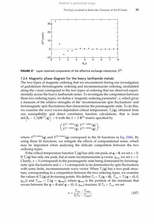
7.2.4 Magnetic phase diagram for the heavy lanthanide metalsThe two types of magnetic ordering that we encountered during our investigationof gadolinium (ferromagnetic ordering and incommensurate ordering, modulatedalong the c-axis) correspond to the two types of ordering that are observed experi-mentally across the heavy lanthanide series. To investigate the competition betweenthese two ordering types, we define a ‘magnetic ordering parameter’, a, which givesa measure of the relative strengths of the ‘incommensurate spin fluctuations’ andferromagnetic spin fluctuations that characterize the paramagnetic state. To do this,we examine the wave vector-dependent critical temperature, Tc(q), obtained fromour susceptibility and direct correlation function calculations, that is fromdet In � 1=3bS 2ð Þ qð Þh i

¼ 0 with the 2 � 2 S(2) matrix specified by

S 2ð Þ�intra qð Þ S 2ð Þ�inter qð ÞS 2ð Þ�inter qð Þ S 2ð Þ�intra qð Þ

� �

;

where S(2)–intra(q) and S(2)–inter(q) correspond to the fit functions in Eq. (106). Byusing these fit functions, we mitigate the effects of computational noise, whichmay be important when analysing the delicate competition between the twoordering types.

If the critical temperature function Tc(q) has only one peak, at q¼ 0, we set a¼ 0.If Tc(q) has only one peak, but at some incommensurate q-vector, qinc, we set a ¼ 1.Clearly, a¼ 0 corresponds to the paramagnetic state being dominated by ferromag-netic spin fluctuations and a ¼ 1 corresponds to its domination by spin fluctuationswith some finite, incommensurate wave vector. When Tc(q) has a two peak struc-ture, corresponding to a competition between the two ordering types, we examinethe values of Tc(q) at its turning points.We define T0¼ Tc(q¼ 0), Tinc¼ Tc(q¼ (0, 0,qinc)) and Tmin ¼ Tc(q ¼ qmin), where qmin is the position of the minimum thatoccurs between the q ¼ 0 and q ¼ (0, 0, qinc) maxima. If T0 > Tinc we set

a ¼ Tinc � Tmin

2 T0 � Tminð Þ ð107Þ

0 1 2 3 4 5 6 7 8

10

0

−10

20

S(2

) (m

eV)

30

Rz/c

FIGURE 37 Layer-resolved components of the effective exchange interaction, S(2).



and if T0 < Tinc, we set

a ¼ 1� T0 � Tmin

2 Tinc � Tminð Þ : ð108Þ

Clearly, a is defined such that a > 0.5 indicates a stronger tendency towardsincommensurate ordering and a < 0.5 indicates a stronger tendency towardsferromagnetic ordering.

In Figure 38, we show a for gadolinium as a function of c/a ratio and unit cellvolume. To account for the difference between the theoretical and experimentalvolumes, the WS-radii in the figure are scaled, such that data shown at theexperimental WS radius of gadolinium corresponds to data calculated at thetheoretical WS-radius. On this phase diagram, we also indicate where the experi-mental lattice parameters of all the heavy lanthanide elements lie, as well as thoseof a Gd–Ho alloy. Since the heavy lanthanide elements differ only in howmany 4felectrons they have, and it is the sd conduction electrons that are responsible formediating the interaction between magnetic moments, gadolinium can be consid-ered a magnetic ‘prototype’ for the post-Gd heavy lanthanide elements. Thus, wepropose that the behaviour of gadolinium as a function of lattice parameters is amodel of all the other heavy lanthanide elements. By considering the phasediagram, Figure 38, as being universal to all heavy lanthanide systems, we predict

Gd

Gd0.55 Ho0.45Tb

1.0

0.8

0.6

0.4

0.2

0.0

3.6

3.7

3.8

3.9

S (

a.u.

)

4.0

c/a1.54 1.58 1.62 1.66

DyHoEr

Tm

FIGURE 38 Ordering parameter, a, for gadolinium as a function of c/a ratio and WS radius.

The black region corresponds to ferromagnetic and the grey region to incommensurate

anti-ferromagnetic spin fluctuations. The experimental lattice parameters of all the heavy

lanthanide elements are indicated by circles; a grey (black) circle indicates that experimentally

the high-temperature ordered state of the element is ferromagnetic (incommensurate

anti-ferromagnetic). The circle for Gd0.55Ho0.45 indicates the experimental lattice

parameters of a Gd–Ho alloy at the critical concentration of Ho at which an incommensurate

anti-ferromagnetic phase first appears. The colour plot can be found in Hughes et al. (2007).



that when going left to right in the heavy lanthanide series, there will be a trendaway from ferromagnetism and towards incommensurate ordering. This isexactly what is observed experimentally, with the magnetic modulation vectorstarting out at zero for gadolinium (ferromagnetic ordering) and then progres-sively increasing through the series to give rise to various incommensurate anti-ferromagnetic structures. From the phase diagram, we predict that the transitionbetween ferromagnetism and incommensurate ordering occurs very rapidly as afunction of c/a ratio, particularly for the higher unit cell volumes. This is consis-tent with recent experimental work on terbium under uniaxial tension. Terbiumexhibits helical ordering and has aWS-radius of 3.724 a.u., with a c/a ratio of 1.580.It has been shown (Andrianov et al., 2000) that by increasing the c/a ratio by aslittle as 0.002 the helical ordering could be completely suppressed. In the phasediagram, the elements dysprosium and terbium are positioned close to, or within,the transition region between ferromagnetic and incommensurate ordering. Thisis consistent with the experimental behaviour of these two systems, which exhibitincommensurate ordering at high temperatures and ferromagnetic ordering atlow temperatures.

Because of their structural similarities, Gd alloys easily with all the other heavylanthanide elements, R0. These alloys transform from ferromagnets to incommen-surate magnetically structured materials once the concentration of R0 exceeds acertain critical concentration xc. We can use the phase diagram to predict thesecritical alloy concentrations. These are listed in Table 11 and are in good agree-ment with experimental values where known.

We can also compute estimates of the magnetic ordering vectors of all theheavy lanthanides from our susceptibility calculations for gadolinium at theappropriate lattice parameters. The results are shown in Figure 39. For example,when we performed a calculation for Gd at the experimental lattice parameters ofterbium (Tb), specified by a c/a ratio of 1.580 and a WS-radius of 3.724 a.u., thesusceptibility peaked at a wave vector q ¼ (0, 0, 0.13), which is in good agreementwith the experimental ordering vector of Tb, (0, 0, 0.11). Overall, we predict agradual increase in the ordering vector across the heavy lanthanide series, inagreement with experiment. We also find that the magnetic ordering vectors of

TABLE 11 Critical alloy concentrations of Gd1�xRx systems

System

Critical concentration, xc

Theoretical Experimental

Gd1�xTbx 0.78Gd1�xDyx 0.56 0.50a

Gd1�xHox 0.49 0.45b

Gd1�xErx 0.45Gd1�xTmx 0.42

a Milstein and Robinson (1967).b Taken from Andrianov and Chistiakov (1997).



the last three members of the series (Ho, Er and Tm) all lie close together, again inagreement with experiment.

Making Gd the prototype for magnetic order in the heavy lanthanides isjustified since the Gd ion has orbital angular momentum L ¼ 0 and so spin-orbitcoupling effects do not need to be incorporated into our calculations. However, ifwe want to infer magnetic transition temperatures for the other heavy lanthanidesfrom our Gd calculations, LS coupling has to be considered. This can be accom-plished by scaling our magnetic transition temperature estimates with the deGennes factor (gJ–1)

2 J(J þ 1) (Blundell, 2001). As shown in the inset ofFigure 39, the transition temperatures obtained from this approach reproducethe experimental trend, although the magnitudes of the temperatures are system-atically underestimated. It is worth noting that when we computed the estimatesof the magnetic ordering vectors, spin-orbit coupling was not important. This isbecause, as argued earlier, the type of magnetic order exhibited by the heavylanthanides is determined by the sd conduction electrons, which are little affectedby spin-orbit coupling and which all the heavy lanthanides have in common.

Overall, the physical picture that emerges from the magnetic ordering phasediagram, Figure 38, links unequivocally the lattice parameters of the heavy

Gd

Tb

Dy

TmHo

Er

0 0.05 0.10 0.15 0.20 0.25Theoretical q {0,0,1}

0.05

0

0.10

0.15

0.20

Exp

erim

enta

l q {

0,0,

1}0.25

0 50 100 150 200 250

100

0

150

200

Exp

. Tor

der (

K)

250

300

Theo. Torder (K)

0.30

FIGURE 39 Experimental magnetic ordering vectors of the heavy lanthanides versus those

predicted from ab initio calculations for gadolinium. The inset shows the corresponding ordering

temperatures. Experimentally Gd has the highest ordering temperature, which decreases mono-

tonically through the heavy lanthanide series.



lanthanides with their magnetic properties. Our results have verified the criticalrole that the c/a ratio plays in determining the magnetic ordering types of theheavy lanthanides and how this is linked to the Fermi surface of the paramagneticphase. However, our discovery that the atomic unit cell volume, associated withthe lattice parameters, is just as important in determining the magnetic propertieshas enabled us to develop a much more complete understanding of heavy lantha-nide magnetism. In particular, we have shown that even when the c/a ratio of aheavy lanthanide system is below the critical value needed for a webbing struc-ture, incommensurate anti-ferromagnetic ordering is not necessarily favouredover ferromagnetic ordering; for incommensurate ordering to win out over ferro-magnetic ordering, the unit cell volume needs to be below a certain value.Experimentally, the unit cell volumes of the heavy lanthanides decrease withincreasing atomic number, in accord with the well-known ‘lanthanide contrac-tion’ (Taylor and Darby, 1972). This contraction occurs because as the number ofelectrons in the poorly shielding 4f orbitals is increased, there is an increase in theeffective nuclear charge and, correspondingly, a decrease in ionic radii. Ourfindings evidently suggest that this contraction helps promote the incommensu-rate ordering in the post-Gd heavy lanthanides. The roles that the different typesof valence electrons play in determining the magnetic structures of the heavylanthanides are thus clear; the itinerant sd electrons, common to all the heavylanthanides, mediate the interaction between magnetic moments and it is thenesting of their Fermi surfaces that can lead to instabilities in the paramagneticphase with respect to the formation of incommensurate spin density waves. Thef electrons, on the other hand, are responsible for setting up the magneticmoments and, as their number increases across the heavy lanthanide series, theyplay an indirect role in promoting the incommensurate ordering by means of thelanthanide contraction.

7.3 Valence fluctuations

As mentioned in Section 7.1, the alloy analogy is a versatile approach that can beapplied to different types of thermal fluctuations. In particular, we will now alsoinclude valence fluctuations. The theoretical framework remains largely as out-lined in the previous section, but the possible configurations at a given site nowinclude the valence state in addition to the direction of the local moment. In thefollowing, this approach will be applied to the finite temperature phase diagramof Ce, focusing on the isostructural a–g transition (Luders et al., 2005). At absolutezero, the two phases can be identified as the tetravalent a-phase at low volumes,and the trivalent g-phase at high volumes. Thus, these phases correspond to adelocalized or localized f-state, respectively. Figure 40 shows the ground stateenergies for different valence configurations, namely the tetravalent f 0 configura-tion, corresponding to an LDA calculation, and SIC-LSD calculations for trivalentf 1 configurations, where f-states with different symmetries are treated as loca-lized, as seen in Table 12. These zero temperature calculations assume a ferro-magnetic alignment of the local moments in the g-phase. However, whendiscussing the finite temperature phase diagram of Ce, we will account for the



paramagnetic state with its disorder of the local moments using the DLM frame-work of Section 7.2. The splittings of the states, shown in Table 12, are due to thecrystal field since in this calculation, the spin-orbit coupling has been neglected.We will later account for spin-orbit coupling through the magnetic entropy terms.Table 12 shows that the state with the A2u symmetry provides the lowest energysolution for the g-phase. Only 0.8 mRy separate the minima of the a- and g-phases,giving rise to the transition pressure at the absolute zero of about�2.3 kbar. This isin good agreement with the experimental value of �7 kbar, when extrapolated tozero temperature, and with other theoretical values. The bulk moduli, given inTable 12, are calculated at the theoretical equilibrium volumes. When evaluated atthe experimental volumes, their values are substantially reduced to 239 kbar forthe a-phase and 203 kbar for the g-phase, which is in considerably better agreementwith the experimental data. The volume collapse is obtained at 22%, which alsocompares well with the experimental values of 14–17%. We note that the underes-timate of the volumes of both the a- and g-phases is mainly due to the KKRl-convergence problem. Although it seems that this l-convergence problem shouldaffect the LSD and SIC-LSD calculations in a similar manner, we observe a

0150 170 190 210 230 250

10

20

30

40

50

LDA

A2u

T2u

T1u

∆E

tot (

mR

y)

V (a.u.)

FIGURE 40 The calculated total energies for Ce from LDA and SIC-LSD, with different f-states

localized, as functions of volume, given in atomic units [(a0)3].

TABLE 12 The total energy differences as obtained from the LDA and SIC-LSD calculations, with

respect to the ground state energy solution (LDA), for Ce in different f-configurations. The

corresponding volumes and bulk moduli (evaluated at the theoretical lattice constants) are also

given

DE (mRy) V (a03) B (kbar)

LDA 0.0 158 701A2u 0.8 202 355

SIC T1u 20.3 201 352T2u 1.5 197 351



significantly larger error for the a-phase. This larger error for the a-phase, which isalso found in the LMTO-ASA calculations, is most likely because LDA is notadequate for describing the correlated nature of the a-phase, as observed inexperiments. In fact, the LDA calculations correspond to the high-pressure a0-phase, which is purely tetravalent and has a smaller lattice constant than theobserved a-phase.

We now return to the description of Ce at finite temperatures. The alloyanalogy for describing the thermal valence and spin fluctuations gives rise to aternary alloy, consisting of Ce atoms with localized f-electrons, described by SIC-LSD, with a concentration of c/2 for each spin direction (spin up and spin down),and Ce atoms with delocalized f-electrons, described by the LDA, with theconcentration (1–c). The free energy of the system is obtained by adding therelevant entropy contributions to the total energy [see Eq. (28)]. The electronicparticle-hole entropy, Sel ¼ �kB

Ð

de n(e)[ fb(e) ln fb(e) þ (1�fb(e)) ln (1�fb(e))], isobtained from the underlying band structure calculations (Nicholson et al., 1994).Here n(e) is the DOS and fb(e) denotes the Fermi distribution. The magneticentropy Smag(c) ¼ kBc ln 6, which corresponds to a spin-orbit coupled state withJ ¼ 5/2, accounting for the magnetic disorder, while the mixing entropy, Smix(c) ¼�kB(c ln c þ (1�c) ln (1�c)), stems from the disorder among the localized anddelocalized Ce atoms. The vibrational entropy, Svib, is assumed to be the same inboth phases and therefore is neglected here. In order to determine the full p–Tphase diagram, it is necessary to calculate the Gibbs free energy:

G T; c; pð Þ ¼ F T; c;V T; c; pð Þð Þ þ p T; c; pð Þ: ð109Þ

From this, at each given pressure and temperature, we can determine the concen-tration of the trivalent Ce, by minimizing the Gibbs free energy with respect to c.

Our calculations go beyond all the earlier work because SIC-LSDA treats all thef-states on equal footing and the KKR-CPA allows for a consistent description ofspin and valence disorder. Johansson et al. (1995) used a binary pseudo-alloyconcept, but needed one adjustable parameter to put on a common energy scaleboth the g-phase, described by LSDA with one f-state included into the core, andthe a-phase, described by the standard LSD approximation, with all the f-statestreated as valence bands. Svane (1996) performed SIC-LSD calculations using asupercell geometry which limited him to the study of a few concentrations only.

We can obtain the free energy of the physical system at a given volume byevaluating the concentration-dependent free energy at the minimizing concentra-tion cmin:

F T;Vð Þ ¼ F T; cmin;Vð Þ: ð110Þ

This free energy, as a function of volume and temperature, is displayed inFigure 41, clearly showing a double-well behaviour for low temperatures, whichgets gradually smoothed out into a single minimum as the temperature isincreased. In addition, it is found that at elevated temperatures the free energyis lowered mainly at large lattice volumes, which is due to the greater entropy ofthe g-phase.



Inserting the minimizing concentration cmin into the pressure–volume relation

p T;Vð Þ ¼ p T; cmin;Vð Þ ¼ � @

@VF T; cmin;Vð Þ ð111Þ

allows one to calculate the isothermal pV-relations of Ce, which are displayed inFigure 42, where it can be seen that the average valence, close to the coexistenceline, gradually changes with increasing temperature. Above the critical tempera-ture, the valence changes continuously with increasing pressure from trivalent totetravalent.

140 160 180 200 220 240

−0.70

−0.69

−0.68

−0.67F

(T,V

) (R

y)

−0.66

V (a.u.)

FIGURE 41 The free energies as function of the volume for the temperatures 0 (highest curve)

and 1800 K (lowest curve) in steps of 100 K.

−20140 160 170150 180 190 200 210 220

V (a.u.)

p (

kbar

)

0

20

40

60

80

100

FIGURE 42 Calculated equation of state of Ce for the temperatures T ¼ 0 (lowest curve), 200,

400, 600, 800, 1000, 1200, 1400, and 1600 K (highest curve). The shading indicates the fraction of

localized electrons: light is all localized (g-phase) and dark is all delocalized (a-phase).



In Figure 43, we present the phase diagram, obtained from the free energies ofthe a–g pseudo-alloy, with the g-phase described by the DLM state. Here, it can beeasily followed how the transition becomes continuous above the critical point.The calculated critical temperature overestimates the experimental value by abouta factor of 2. It is still reasonable considering that the critical temperature is verysensitive to various small details of the calculations and in particular the theoreti-cal lattice parameters of both the a- and g-Ce phases. Also, the calculated slope ofthe phase separation line is slightly too steep, compared to the experimental phasediagram. The likely reason being the overestimate of the volume collapse thatenters the definition of the slope, given by the ratio (Vg�Va)/(Sg�Sa), where Sa(g)and Va(g) are, respectively, values of the entropy and volume of the a(g)-phase atT ¼ 0 K.

Examining in more detail the discontinuity across the phase separation linedisplayed in Figure 44, we find the magnitude of the discontinuities for thevarious contributions to the Gibbs free energy. As expected, all contributionsvanish at the critical temperature, above which there is a continuous cross-overbetween the a- and the g-phase. It can be seen that it is the entropy discontinuitywhich is by far the largest contribution. The phase transition is therefore driven byentropy, rather than by energetics. The entropy discontinuity itself is mainlydetermined by the magnetic entropy.

Summarising this section, we have demonstrated that the alloy analogy offluctuations can be very useful, giving rise to a simple picture of the underlyingphysics, relating the magnetic phase diagram of the late lanthanides to the lantha-nide contraction, and identifying the entropy as the driving force behind the a–gphase transition in Ce. In Section 8, we will outline how this approach can be

0.0

0.2

0.4

0.6

0.8

1.0

1500

1000

T (

K)

500

00 20 40 60 80 100

p (kbar)

FIGURE 43 Phase diagram obtained for the pseudo-alloy, composed of a-Ce (light grey area) and

g-Ce (dark grey area). The grey shades display the fraction of localized electrons. The crosses

indicate the calculated (upper cross) and experimental (lower cross) critical points.



generalized to describe also dynamical, namely quantum, fluctuations, which upto now have been ignored.

8. DYNAMICAL FLUCTUATIONS: THE ‘ALLOY ANALOGY’ AND THELANDAU THEORY OF PHASE TRANSITIONS

Having made use of the ‘alloy analogy’ approach to describe fluctuations indensity functional theories, a number of comments concerning its status in thegeneral theory of condensed-matter are in order. First, it should be stressed thatwhile in the context of phase transitions, such methodology yields an accuratedescription of the high temperature, homogeneous disordered state, and a reliableaccount of its instability at some critical transition temperature Tc, it is seriouslyincomplete for T < Tc as the ground state is approached. Second, one should notfail to mention that there is now a fairly well-developed conceptual framework, adynamical version of the ‘alloy analogy’, in terms of which the shortcomings ofthe above static version near T ! 0 can be understood, and even remedied.

As is well known, there are two ways of approaching the problem of phasetransitions. One of these starts with a study of the ground state and seeks todetermine the critical temperature Tc, at which thermal fluctuations destroy theequilibrium state smoothly connected to it. Usually, at this point either somesymmetry breaking order of the ground state is lost, as in a continuous phasetransitions, or the system becomes an inhomogeneous mixture of coexistingphases as in the cases of the Ce a–g, liquid-gas or other first-order transitions.The alternative to this approach is to start with the high temperature, T > Tc, high

Etot (T)p VT StotT SelT SmixT Smag

T (K)

12

10

8

6

4

2

0

0 400 800 1200 1600

−2

−4

DE

(m

Ry)

FIGURE 44 Discontinuities of the total energy, the total entropy TS, and the pV term over the

phase separation line as function of the temperature. The entropy term is further decomposed

into the electronic, the mixing, and the magnetic contribution.



symmetry, disordered phase, and investigate its stability as the temperature islowered. This is the strategy adopted in a phenomenological Landau Theory(Landau and Lifschitz, 1980). From the point of view of first-principles calcula-tions, the former seems easier as it involves ground state calculations. However,the ‘alloy analogy’ calculations highlighted in this review correspond to the latter.Evidently, in these the role of the CPA is to describe thermal fluctuations ofvarious local electronic configurations and hence the KKR-CPA procedure is anappropriate tool for the study of the high-temperature, high-symmetry equilib-rium states. In fact, when suitably generalized, it can be used for calculating thecoefficients in the Landau expansion of the free energy (Gyorffy et al., 1989) andthereby turning the phenomenological theory into a material specific, quantitativefirst-principles theory.

Examining the accuracy and reliability of the calculations reviewed in Sections7.2 and 7.3 in the light of the above remarks prompts the following observation:the electronic structure relevant to these calculations is a smeared out version ofthat at T ¼ 0. Namely, any coherent fluctuation lasting longer than h/kBT can beassumed to have been averaged to zero and hence such calculations are moreforgiving than those near T¼ 0 where timescales much longer than h/kBTc need tobe accounted for. Thus, the first-principles Landau Theory alluded to above can beconsidered a robust and efficient theory of the phase diagrams. By contrast forT < Tc, as T tends to 0, longer and longer timescales make their presence felt and amore accurate description of the many-electron problem becomes necessary.

A particular general shortcoming of the ‘alloy analogy’ approximation is that itcannot describe quantum fluctuations such as the zero point fluctuations of spinwaves. Evidently, these can be important at and near T ¼ 0. Moreover, anensemble average of static fluctuations depicted by the ‘alloy’ configurationswill, within the CPA, inevitably lead to quasi-particles with finite lifetime evenat T ¼ 0. Namely, the ground state is generically not that of a Fermi liquid as itmostly should be. In what follows we shall summarize briefly the current state ofconceptual framework that needs to be invoked to deal with these issues.

In condensed matter at a site, an electron scatters from both the atomic nucleiand the other electrons in its vicinity. Such ‘target’ is not, in general, a static, spin-dependent electrostatic, c-number potential but a time-dependent quantummechanical object which recoils during the scattering process. Clearly, the fullcomplexity of scattering events produced by such ‘targets’ are not described bythe static mean field theory language of the ‘alloy analogy’. However, it turns outthat their essence is adequately captured by a dynamical generalization of thiswell tried methodology, namely the DMFT (Georges et al., 1996). Like the ‘alloyanalogy’, this elegant procedure focuses on the single site nature of the many-electron problem in solids and it can be viewed as a time-dependent CPA in whichthe potential seen by an electron at a site changes with time during the scatteringprocess and the averaging over configurations becomes average over all historiesof such variations (Kakehashi, 2002).

A remarkable consequence of introducing time-dependent one-electron poten-tials into the calculation is that the well-known instability of a degenerate Fermisystem to sudden local perturbations (Anderson, 1967) comes into play. This



effect, which is well understood in the context of the X-ray edge-singularity(Nozieres and DeDominicis, 1969) and the Kondo (Anderson et al., 1970) pro-blems, leads to qualitatively new features in the one-electron spectra predicted bythe DMFT compared with the consequences of the static CPA-based theories. Themost spectacular of these is the central peak, arising from the Kondo resonance atthe Fermi energy, between the upper and lower Hubbard bands, which arealready evident in the static alloy analogy calculations. As physical consequencesof this peak, one might mention its role in the explanation of the metal-insulatorMott transition (Georges et al., 1996) and the spin-polarization Kondo cloud thatscreens magnetic impurities in dilute alloys (Anderson et al., 1970). Indeed, it mayvery well be relevant to the Ce a–g transition discussed in Section 7.3 (Held et al.,2001).

Since their invention in the early 1990s, the DMFT technique (Georges et al.,1996) and its cluster generalization DCA (Hettler et al., 1998) have been studiedintensively and have been successfully applied to many different problems inmetal physics. But, while its virtues and limitations are well documented forsimple tight binding model Hamiltonians, its implementation within the contextof a fully first-principles theory remains an aspiration only. What has been done,repeatedly and with considerable success, is what may be called the LDA þ U þDMFT method (Georges et al., 1996). In these calculations, the LDA þ U part is amethod for generating an effective, usually a multi-band Hubbard, Hamiltonianwhich serves as input into a DMFT procedure, but there is rarely an effort torecalculate the LDA bands (site energies and hopping integrals) or the electron–electron interaction parameter U with the view of iterating to self-consistency.Strangely, although technically the problem appears to be difficult conceptually,thanks to the numerous analytical and numerical results mentioned above, it isrelatively simple. The fluctuations to be captured by the putative theoreticalframework are tunnelling between atomic-like local electronic configurations,and of these, there are only few that are degenerate in energy and hence can bethe source of a Kondo-like resonance. In other words, at an atomic centre, anelectron scatters from a quantummechanical two or few level systems instead of aclassical effective electrostatic potential. Scaling arguments suggest that the occur-rences of such resonances are general consequences of degenerate Fermi systemsbeing perturbed by sudden, local, quantum perturbations and their width is anew, emergent, low-energy scale kBTK where TK is usually referred as the ‘Kondo’temperature (Cox and Zawadowski, 1999). From the point of view of our presentconcern, the importance of these results are twofold. First, this low-energy scale,which governs the behaviour of low-temperature fluctuations, has no counterpartin the static mean field theory. Second, kBTK varies dramatically from material tomaterial from 1 to 1000 K. Thus, there is need for a sophisticated first-principlestheory which can make quantitative material specific predictions of kBTK. Clearly,if TK Tc for some particular order, the high-temperature phase is well describedby the ensemble of static fluctuations depicted in the ‘alloy analogy’ calculation.On the other hand, if TK � Tc, the static calculations miss out important aspectsof the physics. To highlight the burden of this remark, we note that the Curietemperatures of ferromagnets and the critical temperatures of the conventional



superconductors can be calculated fairly reliably for the majority of materials.Evidently, the challenge here is to do the same for kBTK.

9. CONCLUSIONS

This chapter has given an ab initio justification for the dual, localized and band-like, character of the 4f-states in the lanthanides. The SIC-LSD provided thefirst-principles band theory scheme allowing for this differentiation betweenband-like, where the gain in band formation energy dominates, and localized 4felectrons, where the gain in localization energy dominates. From this, the notionof nominal valence was developed defining the number of remaining band-likestates as the valence of the lanthanide ion. These band-like states determine thebonding properties. This definition of valence turned out to be extremely usefuland in Section 4, we gave numerous examples how this notion of valence con-tributed to a better understanding of the physical properties of the lanthanidesand their compounds. In particular, the bonding properties of the lanthanides,such as the lattice constants, and their pressure behaviour could be studiedwithout using adjustable parameters. Local magnetic moments and spectroscopicinvestigations provided a study of some of the properties of the localized f-states.Specifically, we found the degree of 4f localization to be similar in the light andheavy lanthanides. The one-electron SIC-LSD is shown to be an ab initio computa-tional scheme consistent with all three Hund’s rules.

A finite temperature generalization based on the LSIC-LSD method led to thefirst-principles study of the phase diagrams of the lanthanides. The study of amagnetic phase diagram for the heavy lanthanides led to the discovery of the roleplayed by the lanthanide contraction in determining the magnetic structure ofheavy lanthanides. Also, the importance of the Fermi surface webbing features indriving the magnetic order was explained. Calculating the phase diagram of thea–g phase transition in elemental Ce allowed us to identify the entropy as thedriving force in this transition. These finite temperature studies incorporatedthermal fluctuations only. Finally, an outline was given on how to include dyna-mical, quantum, fluctuations in the present methodology.

REFERENCES

Aerts, C.M., Strange, P., Horne, M., Temmerman, W.M., Szotek, Z., Svane, A. Phys. Rev. B 2004, 69,045115.

Ahuja, R., Auluck, S., Johansson, B., Brooks, M.S.S. Phys. Rev. B 1994, 50(8), 5147–5154.Alameda, J.M., Givord, D., Lemaire, R., Lu, Q., Palmer, S.B., Tasset, F. J. Phys. 1982, 43, 133.Amadon, B., Biermann, S., Georges, A., Aryasetiawan, F. Phys. Rev. Lett. 2006, 96, 066402.Anderson, P.W. Phys. Rev. Lett. 1967, 18, 1049.Andersen, O.K. Phys. Rev. B 1975, 12, 3060.Andersen, O.K., Jepsen, O., Glotzel, D. in: Bassani, F., Fumi, F., Tosi, M.P., editors. Highlights

of CondensedMatter Theory, International School of Physics Enrico Fermi, Course 89, Amsterdam:North Holland; 1989, p. 59.

Anderson, P.W., Yuval, G., Haman, D.R. Phys. Rev. B 1970, 1, 4464.



Andrianov, A.V. J. Magn. Magn. Mater. 1995, 140–144, 749.Andrianov, A.V., Chistiakov, O.D. Phys. Rev. B 1997, 55, 14107.Andrianov, A.V., Kosarev, D.I., Beskrovnyi, A.I. Phys. Rev. B 2000, 62, 13844.Anisimov, V.I., Gunnarsson, O. Phys. Rev. B 1991, 43, 7570.Anisimov, V.I., Aryasetiawan, F., Lichtenstein, A.I. J. Phys.: Condens. Matter 1997, 9, 767.Anisimov, V.I., Zaanen, J., Andersen, O.K. Phys. Rev. B 1991, 44, 943.Anisimov, V.I., Solovyev, I.V., Korotin, M.A., Czyzyk, M.T., Sawatzky, G.A. Phys. Rev. B 1993, 48,

16929.Antonov, V.N., Yaresko, A.N., Perlov, A.Y., Thalmeier, A., Fulde, P., Oppeneer, P.M., Eschrig, H. Phys.

Rev. B 1998, 58, 9752–9762.Arola, E., Strange, P. Appl. Phys. A 2001, 73, 667.Arola, E., Strange, P., Gyorffy, B.L. Phys. Rev. B 1997, 55, 472.Arola, E., Horne, M., Strange, P., Winter, H., Szotek, Z., Temmerman, W.M. Phys. Rev. B 2004, 70,

235127.Aryasetiawan, F., Gunnarsson, O. Phys. Rev. B 1994, 49, 16214.Aryasetiawan, F., Gunnarsson, O. Rep. Prog. Phys. 1998, 61, 237.Banister, J.R., Legvold, S., Spedding, F.H. Phys. Rev. 1954, 94, 1140.Becke, A.D. J. Chem. Phys. 1993, 98, 5648.Beiden, S.V., Temmerman, W.M., Szotek, Z., Gehring, G.A. Phys. Rev. Lett. 1997, 79, 3970.Benedict, U., Holzapfel, W.B. in: Gschneidner, K.A., Eyring, L., Lander, G.H., Choppin, G.R., editors.

Handbook on the Physics and Chemistry of Rare Earths. vol. 17, Amsterdam: North-Holland; 1993,chap. 113.

Bianconi, A., Kotani, A., Okada, K., Giorgi, R., Gargano, A., Marcelli, A., Miyahara, K. Phys. Rev. B1988, 38, 3433.

Bihan, T.L., Darracq, S., Heathman, S., Benedict, U., Mattenberger, K., Vogt, O. J. Alloys Compd. 1995,226, 143.

Blanter, Y.M., Kaganov, M.I., Pantsulaya, A.V., Varlamov, A.A. Phys. Rep. 1994, 245, 159.Blume, M. J. Appl. Phys. 1985, 57, 3615.Blume, M., Gibbs, D. Phys. Rev. B 1988, 37, 1779.Blundell, S. 2001. Magnetism in Condensed Matter, Oxford: Oxford University Press.Bonville, P., Hammann, J., Hodges, J.A., Imbert, P., Jehanno, G.J. Phys. Rev. Lett. 1986, 57, 2733.Boothroyd, A.T., Gardiner, C.H., Lister, S.J.S., Santini, P., Noailles, B.D.R.L.D., Currie, D.B.,

Eccleston, R.S., Bewleya, R.I. Phys. Rev. Lett. 2001, 86, 2082.Bouhemadou, A., Khenata, R., Sahnoun, M., Baltache, H., Kharoubi, M. Physica B 2005, 363, 255.Brown, S.D., Strange, P., Bouchenoire, L., Zarychta, B., Thompson, P., Mannix, D., Stockton, S.,

Horne, M., Arola, E., Ebert, H., Szotek, Z., Temmerman, W.M., Fort, D. Phys. Rev. Lett 2007, 99,247401.

Butorin, S.M., Duda, L.-C., Guo, J.-H., Wassdahl, N., Nordgren, J., Nakazawa, M., Kotani, A. J. Phys.:Condens. Matter. 1997, 9, 8155.

Campagna, M., Bucher, E., Wertheim, G.K., Buchanan, D.N.E., Longinotti, L.D. Phys. Rev. Lett. 1974a,32, 885.

Campagna, M., Bucher, E., Wertheim, G.K., Longinotti, L.D. Phys. Rev. Lett. 1974b, 33, 165.Campagna, M., Wertheim, G.K., Baer, Y. in: Ley, L., Cardona, M., editors. Photoemission in Solids.

vol. II. Berlin: Springer; 1979, chap. 4.Ceperley, D.M., Alder, B.J. Phys. Rev. Lett. 1980, 45, 566–569.Chainani, A., Kumigashira, H., Ito, T., Sato, T., Takahashi, T., Yokoya, T., Higuchi, T., Takeuchi, T.,

Shin, S., Sato, N.K. Phys. Rev. B 2002, 65, 155201.Chantis, A.N., van Schilfgaarde, M., Kotani, T. Phys. Rev. B 2007, 76, 165126.Cho, E.-J., Chung, J.-S., Oh, S.-J., Suga, S., Taniguchi, M., Kakizaki, A., Fujimori, A., Kato, H.,

Miyahara, T., Suzuki, T., Kasuya, T. Phys. Rev. B 1993, 47, 3933.Cowan, R.D. Phys. Rev. 1967, 163, 54.Cox, D.I., Zawadowski, A. Exotic Kondo Effects in Metals, London: Taylor and Francis; 1999.Cracknell, A.P., Wong, K.C. The Fermi Surface, Oxford: Clarendon; 1973.Crisan, V., Entel, P., Ebert, H., Akai, H., Johnson, D.D., Staunton, J.B. Phys. Rev. B 2002, 66(1), 014416.Croft, M., Jayaraman, A. Solid State Commun. 1980, 35, 203.



Crowe, S.J., Dugdale, S.B., Major, Z., Alam, M.A., Duffy, J.A., Palmer, S.B. Europhys. Lett. 2004, 65, 235.Debray, D., Werner, A., Decker, D.L., Loewenhaupt, M., Holland-Moritz, E. Phys. Rev. B 1982, 25, 3841.Degiorgi, L., Bacsa, W., Wachter, P. Phys. Rev. B 1990, 42, 530.Degiorgi, L., Teraoka, S., Compagnini, G., Wachter, P. Phys. Rev. B 1993, 47, 5715.Delin, A., Fast, L., Johansson, B., Wills, J.M., Eriksson, O. Phys. Rev. Lett. 1997, 79(23), 4637–4640.Delin, A., Fast, L., Johansson, B., Eriksson, O., Wills, J.M. Phys. Rev. B 1998, 58, 4345–4351.Dimmock, J.O., Freeman, A.J. Phys. Rev. Lett. 1964, 13(25), 750–752.Divis, M., Rusz, J. J. Magn. Magn. Mater. 2005, 290–291, 1015.Dobrich, K.M., Bihlmayer, G., Starke, K., Prieto, J.E., Rossnagel, K., Koh, H., Rotenberg, E., Blugel, S.,

Kaindl, G. Phys. Rev. B 2007, 76, 035123.Dreizler, R.M., Gross, E.K.U. Density Functional Theory, Berlin: Springer-Verlag; 1990.Duan, C.-G., Sabirianov, R.F., Mei, W.N., Dowben, P.A., Jaswal, S.S., Tsymbal, E.Y. J. Phys.: Condens.

Matter 2007, 19, 315220.Dugdale, S.B., Fretwell, H.M., Alam, M.A., Kontrym-Sznajd, G., West, R.N., Badrzadeh, S. Phys. Rev.

Lett. 1997, 79(5), 941–944.Duthie, J.C., Pettifor, D.G. Phys. Rev. Lett. 1977, 38(10), 564–567.Eriksson, O., Brooks, M.S.S., Johansson, B. J. Less Common. Met. 1990a, 158, 207.Eriksson, O., Brooks, M.S.S., Johansson, B. Phys. Rev. B. 1990b, 41, 7311–7314.Eriksson, O., Brooks, M.S.S., Johansson, B., Albers, R.C., Boring, A.M. J. Appl. Phys. 1991, 69, 5897–5902.Eriksson, O., Ahuja, R., Ormeci, A., Trygg, J., Hjortstam, O., Soderlind, P., Johansson, B., Wills, J.M.

Phys. Rev. B 1995, 52, 4420.Eschrig, H., Sargolzaei, M., Koepernik, K., Richter, M. Europhys. Lett. 2005, 72, 611–617.Eyring, L. in: Gschneidner Jr., K.A., Eyring, L., editors. Handbook on the Physics and Chemistry of

Rare Earths. vol. 3. Amsterdam: North-Holland; 1978, chap. 9.Faulkner, J.S. Prog. Mater. Sci 1982, 27, 1.Faulkner, J.S., Stocks, G.M. Phys. Rev. B 1981, 23, R5628.Feynman, R.P. Phys. Rev. 1955, 97, 660.Filip, A.T., LeClair, P., Smitts, C.J.P., Kohlhepp, J.T., Swagten, J.M., Koopmans, B., de Jonge, W.J.M.

Appl. Phys. Lett. 2002, 81, 1815.Freeman, A.J., Min, B.I., Norman, M.R. in: Eyring Jr., K.A.L., Hufner, S., editors. Handbook on the

Physics and Chemistry of Rare Earths. vol. 10, pp. 165–229. Amsterdam Elsevier; 1987.Fretwell, H.M., Dugdale, S.B., Alam, M.A., Hedley, D.C.R., Rodriguez-Gonzalez, A., Palmer, S.B. Phys.

Rev. Lett. 1999, 82(19), 3867–3870.Fujimori, A. Phys. Rev. B 1983, 28, 4489.Gardiner, C.H., Boothroyd, A.T., Pattison, P., McKelvy, M.J., McIntyre, G.J., Lister, S.J.S. Phys. Rev. B

2004, 70, 024415.Gasiorowicz, S. Quantum Physics, New York: John Wiley and Sons; 1974.Georges, A., Kotliar, G., Krauth, W., Rozenberg, M.J. Rev. Mod. Phys. 1996, 68, 13.Gerward, L., Olsen, J.S., Petit, L., Vaitheeswaran, G., Kanchana, V., Svane, A. J. Alloys Compd. 2005,

400, 56.Ghosh, D.B., De, M., De, S.K. Phys. Rev. B 2003, 67, 035118.Godby, R.W., Schluter, M., Sham, L.J. Phys. Rev. B 1988, 37, 10159.Gotsis, H.J., Mazin, I.I. Phys. Rev. B 2003, 68, 224427.Gschneidner Jr., K.A. J. Less-Common Met. 1969, 17, 13.Gschneidner Jr., K.A. J. Less-Common. Met. 1971, 25, 405.Gschneidner Jr., K.A. J. Alloys Compds. 1993, 192, 1.Gyorffy, B.L., Stott, M.J. in: Fabian, D.J., Watson, L.M., editors. Band Structure Spectroscopy of Metals

and Alloys, New York: Academic Press; 1973.Gyorffy, B.L., Stocks, G.M. in: Phariseau, P., Gyorffy, B.L., Scheire, L., editors. Electrons in Disordered

Metals and at Metallic Surfaces, vol. 42 of NATO ‘ASI Series Physics B’, NewYork: Plenum Press;1978.

Gyorffy, B.L., Pindor, A.J., Staunton, J., Stocks, G.M., Winter, H. J. Phys. F-Met. Phys. 1985, 15(6),1337–1386.

Gyorffy, B.L., Johnson, D.D., Pinski, F.J., Nicholson, D.M., Stocks, G.M. in: Stocks, G.M., Gonis, A.,editors. Alloy Phase Stability, pp. 421–468. Dordrecht, Kluwer Academic Publisher; 1989.



Hanyu, T., Ishii, H., Yanagihara, M., Kamada, T., Miyahara, T., Kato, H., Naito, K., Suzuki, S., Ishii, T.Solid State Commun. 1985, 56, 381.

Harmon, B.N., Antropov, V.P., Lichtenstein, A.I., Solovyev, I.V., Anisimov, V.I. J. Phys. Chem. Solids1995, 56, 1521–1524.

Hassan, A.K., Levy, L.P., Darie, C., Strobel, P. Phys. Rev. B 2003, 67, 214432.Haule, K., Oudovenko, V., Savrasov, S.Y., Kotliar, G. Phys. Rev. Lett. 2005, 94, 036401.Havinga, E.E., Buschow, K.H.J., van Daal, H.J. Solid State Commun. 1973, 13, 621.Hedin, L. Phys. Rev. A 1965, 139, 796.Heinemann, M., Temmerman, W.M. Phys. Rev. B 1994, 49(6), 4348–4351.Held, K. Adv. Phys. 2007, 56, 829.Held, K., McMahan, A.K., Scalettar, R.T. Phys. Rev. Lett. 2001, 87, 276404.Hettler, M.H., Tahvildar-Zadeh, A.N., Jarrell, M., Pruschke, T., Krishnamurthy, H.R. Phys. Rev. B 1998,

58, 7475.Hill, J.P., McMorrow, D.F. Acta Crystallogr. A 1996, 52, 236.Hirosaki, N., Ogata, S., Kocer, C. J. Alloys Compd. 2003, 351, 31.Hoekstra, H.R., Gingerich, K.A. Science 1964, 146, 1163.Hohenberg, P., Kohn, W. Phys. Rev. 1964, 136, B864–B871.Holland-Moritz, N. Z. Phys. B: Condens. Matter 1992, 89, 285.Horne, M., Strange, P., Temmerman, W.M., Szotek, Z., Svane, A., Winter, H. J. Phys.: Condens. Matter

2004, 16, 5061.Hubbard, J. Proc. R. Soc. London, Ser. A 1963, 276, 238.Hubbard, J. Proc. R. Soc. London, Ser. A 1964a, 277, 237.Hubbard, J. Proc. R. Soc. London, Ser. A 1964b, 281, 401.Hughes, I.D., Dane, M., Ernst, A., Hergert, W., Luders, M., Poulter, J., Staunton, J.B., Svane, A.,

Szotek, Z., Temmerman, W.M. Nature 2007, 446(7136), 650–653.Hulliger, F. in: Gschneidner Jr., K.A., Eyring, L., editors. Handbook on the Physics and Chemistry of

Rare Earths. vol. 4. Amsterdam: North-Holland; 1979, chap. 33.Hybertsen, M.S., Louie, S.G. Phys. Rev. B 1986, 34, 5390.Iandelli, A., Franceschi, E. J. Less-Common. Met. 1973, 30, 211.Iandelli, A., Olcese, G.L., Palenzona, A. J. Less-Common. Met. 1980, 76, 317.Ito, T., Chainani, A., Takahashi, H.K.T., Sato, N.K. Phys. Rev. B 2002, 65, 155202.Jackson, C. Phys. Rev. 1969, 178, 949.Jayaraman, A. in: Gschneidner Jr., K.A., Eyring, L., editors. Handbook on the Physics and Chemistry of

Rare Earths. vol. 1. Amsterdam: North-Holland; 1978, chap. 9.Jayaraman, A., Singh, A.K., Chatterjee, A., Devi, S.U. Phys. Rev. B 1974, 9, 2513.Jayaraman, A. in: Gschneidner Jr., K.A., Eyring, L., editors. Handbook on the Physics and Chemistry of

Rare Earths. vol. 2. Amsterdam: North-Holland; 1979, chap. 20.Jensen, J., Mackintosh, A.K. Rare Earth Magnetism, Oxford: Clarendon; 1991.Johansson, B., Rosengren, A. Phys. Rev. B. 1975, 11, 2836–2857.Johnson, D.D., Nicholson, D.M., Pinski, F.J., Gyorffy, B.L., Stocks, G.M. Phys. Rev. Lett. 1986, 56(19),

2088–2091.Johansson, B., Abrikosov, I.A., Alden, M., Ruban, A.V., Skriver, H.L. Phys. Rev. Lett. 1995, 74, 2335.Jones, R.O., Gunnarsson, O. Rev. Mod. Phys. 1989, 61, 689.Joyce, J.J., Andrews, A.B., Arko, A.J., Bartlett, R.J., Blythe, R.I.R., Olson, C.G., Benning, P.J., Canfield, P.

C., Poirier, D.M. Phys. Rev. B 1996, 54, 17515.Kakehashi, Y. Phys. Rev. B. 2002, 66, 104428.Karnatak, R.C., Esteva, J.-M., Dexpert, H., Gasgnier, M., Caro, P.E., Albert, L. Phys. Rev. B 1987, 36,

1745.Kasuya, T. Prog. Theor. Phys. 1956, 16.Kasuya, T. J. Phys. Soc. Japan 1994, 63, 843.Keeton, S.C., Loucks, T.L. Phys. Rev. 1968, 168, 672.Kern, S., Loong, C.-K., Faber Jr, J.Jr, Lander, G.H. Solid State Commun. 1984, 49, 295.Kittel, C. Introduction to Solid State Physics 6th edition New York: John Wiley and Sons; 1986.Koelling, D.D., Boring, A.M., Wood, J.H. Solid State Commun. 1983, 47, 227.Kohn, W., Rostoker, N. Phys. Rev. 1954, 94, 1111.



Kohn, W., Sham, L.J. Phys. Rev. 1965, 140, A1133–A1138.Korringa, J. Physica 1947, 13, 392.Kotliar, G., Savrasov, S.Y., Haule, K., Oudovenko, V.S., Parcollet, O., Marianetti, C.A. Rev. Mod. Phys.

2006, 78, 865.Krill, G., Ravet, M.F., Kappler, J.P., Abadli, L., Leger, J.M., Yacoubi, N., Loriers, C. Solid State Commun.

1980, 33, 351.Krutzen, B.C.H., Springelkamp, F. J. Phys.: Condens. Matter 1989, 1, 8369.Kubler, J. International Series of Monographs on Physics, vol. 106 Oxford University Press; 2000.Kubler, J., Eyert, V. in: Cahn, R.W., Haasen, P., Kramer, E.J., editors. Materials Science and Technol-

ogy. vol. 3a, p. 1. New York: Weinheim; 1993.Kumar, R.S., Cornelius, A.L., Svane, A., Vaitheeswaran, G., Kanchana, V., Bauer, E.D., Hu, M., Nicol, F.

Phys. Rev. B. 2008, 78, 075117.Kurz, P., Bihlmayer, G., Blugel, S. J. Phys. Condens. Matter 2002, 14, 6353.Lægsgaard, J., Svane, A. Phys. Rev. B 1998, 58, 12817.Lal, H.B., Gaur, K. J. Mater. Sci. 1988, 23, 919.Landau, L.D., Lifschitz, E.M. Course of Theoretical Physics, vol. 5, 3rd edition. Oxford: Pergamon; 1980.Lang, J.K., Baer, Y., Cox, P.A. J. Phys. F 1981, 11, 121.Langford, H.D., Temmerman, W.M., Gehring, G.A. J. Phys.: Condens. Matter 1990, 2, 559.Larson, P., Lambrecht, W.R.L., Chantis, A.N., van Schilfgaarde, M. Phys. Rev. B 2007, 75, 045114.Lebegue, S., Santi, G., Svane, A., Bengone, O., Katsnelson, M.I., Lichtenstein, A.I., Eriksson, O. Phys.

Rev. B 2005, 72, 245102.Lebegue, S., Svane, A., Katsnelson, M.I., Lichtenstein, A.I., Eriksson, O. Phys. Rev. B 2006a, 74, 045114.Lebegue, S., Svane, A., Katsnelson,M.I., Lichtenstein, A.I., Eriksson, O. J. Phys.: Condens.Matter 2006b,

18, 6329.LeClair, P., Ha, J.K., Swagten, H.J.M., van de Vin, C.H., Kohlhepp, J.T., de Jonge, W.J.M. J. Appl. Phys.

2002, 80, 625.Leger, J.M. Physica B 1993, 190, 84.Leger, J.M., Aimonino, P., Loriers, J., Dordor, P., Coqblin, B. Phys. Lett. 1980, 80A, 325.Leger, J.M., Epain, R., Loriers, J., Ravot, D., Rossat-Mignod, J Phys. Rev. B 1983, 28, 7125.Leger, J.M., Ravot, D., Rossat-Mignod, J. J. Phys. C 1984, 17, 4935.Leger, J.M., Oki, K., Rossat-Mignod, J., Vogt, O. J. Phys. 1985, 46, 889.Leger, J.M., Redon, A.M. J. Less-Common. Met. 1989, 156, 137.Lehner, C., Richter, M., Eschrig, H. Phys. Rev. B 1998, 58, 6807.Li, D.X., Oyamada, A., Hashi, K., Haga, Y., Matsumara, T., Shida, H., Suzuki, T., Kasuya, T., Donni, A.,

Hulliger, F. J. Magn. Magn. Mater 1995, 140–144, 1169.Lichtenstein, A.I., Anisimov, V.I., Zaanen, J. Phys. Rev. B 1995, 52, R5467–5470.Lichtenstein, A.I., Katsnelson, M.I. Phys. Rev. B 1998, 57, 6884.Lifshitz, I.M. Sov. Phys. JETP 1960, 11, 1130.Lindgren, I. Int. J. Quantum Chem. 1971, 5, 411.Ling, M.F., Staunton, J.B., Johnson, D.D. Europhys. Lett. 1994, 25(8), 631–636.Lloyd, P., Best, P.R. J. Phys. C-Solid State Phys. 1975, 8, 3752.Loschen, C., Carrasco, J., Neyman, K.M., Illas, F. Phys. Rev. B 2007, 75, 035115.Lovesey, S.W., Collins, S.P. X-ray Scattering and Absorption by Magnetic Materials, Oxford: Clarendon;

1996.Luders, M., Ernst, A., Dane, M., Szotek, Z., Svane, A., Kodderitzsch, D., Hergert, W., Gyorffy, B.L.,

Temmerman, W. Phys. Rev. B 2005, 71(20), 205109.Mahan, G.D. Many-Particle Physics, New York: Plenum Press; 1990.Marabelli, F., Wachter, P. Phys. Rev. B 1987, 36, 1238.Martin, R.M. Electronic Structure: Basic Theory and Practical Methods, Cambridge: Cambridge

Universtiy Press 2004.Mattocks, P.G., Young, R.C. J. Phys. F 1977, 7, 1219.McMahan, A.K., Held, K., Scalettar, R.T. Phys. Rev. B 2003, 67, 075108.Mermin, N.D. Phys. Rev. 1965, 137, A1441.Messiah, A. Quantum Mechanics, Amsterdam North Holland; 1965.Milstein, F., Robinson, L.B. Phys. Rev. 1967, 159, 466.



Mirone, A. Eur. J. Phys. B: Condens. Matter Complex Syst. 2005, 47, 509.Moewes, A., Ederer, D.L., Grush, M.M., Callcott, T.A. Phys. Rev. B 1999, 59, 5452.Mohn, P., Persson, C., Blaha, P., Schwarz, K., Novak, P., Eschrig, H. Phys. Rev. Lett. 2001, 87, 196401.Moodera, J.S., Meservey, R., Hao, X. Phys. Rev. Lett. 1993, 70, 853.Mori, N., Okayama, Y., Takahashi, H., Haga, Y., Suzuki, T. Physica B 1993, 186–188, 444.Moriya, T. Solid State Sciences, vol. 29, Springer Series Berlin and New York: Springer; 1981.Nicholson, D.M.C., Stocks, G.M., Wang, Y., Szotek, Z., Temmerman,W.M. Phys. Rev. B 1994, 50, 14686.Nordstrom, L., Mavromaras, A. Europhys. Lett. 2000, 49, 775.Nozieres, P., DeDominicis, C. Phys. Rev. 1969, 178, 1097.Ogasawara, H., Kotani, A., Okada, K., Thole, B.T. Phys. Rev. B 1991, 43, 854.Oh, S.-J., Allen, J.W. Phys. Rev. B 1984, 29, 589.Ono, S., Hui, F.L., Despault, J.G., Calvert, L.D., Taylor, J.B. J. Less-Common. Met. 1971, 25, 287.Oppeneer, P.M., Antonov, V.N., Yaresko, A.N., Perlov, A.Y., Eschrig, H. Phys. Rev. Lett. 1997, 78, 4079.Ott, H.R., Rudigier, H., Hulliger, F. Solid State Commun. 1985, 55, 113.Oyamada, A., Hashi, K., Maegawa, S., Goto, T., Li, D.X., Suzuki, T., Donni, A., Hulliger, F. Physica B

1994, 199 & 200, 42.Pederson, M.R., Heaton, R.A., Lin, C.C. J. Chem. Phys. 1984, 80, 1972.Pederson, M.R., Heaton, R.A., Lin, C.C. J. Chem. Phys. 1985, 82, 2688.Perdew, J.P., Zunger, A. Phys. Rev. B 1981, 23, 5048.Perdew, J.P., Wang, Y. Phys. Rev. B 1992, 45, 13244–13249.Petit, L., Svane, A., Szotek, Z., Temmerman, W.M. Phys. Rev. B 2005, 72, 205118.Petit, L., Svane, A., Szotek, Z., Temmerman, W.M. in: Fanciulli, M., Scarel, G., editors. Topics in

Applied Physics, vol. 106, p. 331. Berlin Heidelberg: Springer-Verlag; 2007.Petukhov, A.G., Mazin, I.I., Chioncel, L., Lichtenstein, A.I. Phys. Rev. B 2003, 67, 153106.Pickett, W.E., Koelling, D.D., Freeman, A.J. Phys. Rev. B 1981, 23, 1266.Pollak, R.A., Holtzberg, F., Freeouf, J.L., Eastman, D.E. Phys. Rev. Lett. 1974, 33, 820.Prokofiev, A.V., Shelyakh, A.I., Melekh, B.T. J. Alloys Compd. 1996, 242, 41.Razee, S.S.A., Staunton, J.B., Szunyogh, L., Gyorffy, B.L. Phys. Rev. Lett. 2002, 88(14), 147201.Rhyne, J.J., McGuire, T. IEEE Trans. Magn. 1972, MAG-8, 105.Richter, M., Eschrig, H. Solid State Commun. 1989, 72, 263.Rinke, P., Scheffler, M., Qteish, A., Winkelnkemper, M., Bimberg, D., Neugebauer, J. Appl. Phys. Lett.

2006, 89, 161919.Robinson, R.A., Purwanto, A., Kohgi, M., Canfield, P.C., Kamiyami, T., Ishigaki, T., Lynn, J.W.,

Erwin, R., Peterson, E., Movshovich, R. Phys. Rev. B 1994, 50, 9595.Ruderman, M.A., Kittel, C. Phys. Rev. 1954, 96, 99.Sakai, O., Shimuzi, Y., Kaneta, Y. J. Phys. Soc. Jpn. 2005, 74, 2517.Sakai, O., Shimuzi, Y. J. Phys. Soc. Jpn. 2007, 76, 044707.Sakon, T., Sato, N., Oyamada, A., Takeda, N., Suzuki, T., Komatsubara, T. J. Phys. Soc. Jpn. 1992, 61,

2209.Sandratsakii, L.M., Kubler, J. Europhys. Lett 1993, 23, 661.Scarel, G., Svane, A., Fanciulli, M. in: Fanciulli, M., Scarel, G., editors. Topics in Applied Physics,

vol. 106, p. 1. Berlin Heidelberg: Springer-Verlag; 2007.Schirber, J.E., Schmidt, F.A., Harmon, B.N., Koelling, D.D. Phys. Rev. Lett. 1976, 36(8), 448–450.Schußler-Langeheine, C., Weschke, E., Mazumdar, C., Meier, R., Grigoriev, A.Y., Kaindl, G., Sutter, C.,

Abernathy, D., Grubel, G., Richter, M. Phys. Rev. Lett. 2000, 84(24), 5624–5627.Shirotani, I., Hayashi, J., Yamanashi, K., Hirano, K., Adachi, T., Ishimatsu, N., Shimomura, O.,

Kikegawa, T. Physica B 2003, 334, 167.Sidorov, V.A., Stepanov, N.N., Khvostantsev, L.G., Tsiok, O.B., Golubkov, A.V., Oskotski, V.S.,

Smirnov, I.A. Semicond. Sci. Technol. 1989, 4, 286.Silva, J.L.F.D., Ganduglia-Pirovano, M.V., Sauer, J., Bayer, V., Kresse, G. Phys. Rev. B 2007, 75, 045121.Singh, D.J. Phys. Rev. B 1991, 44(14), 7451–7454.Sinha, S.K. in: Gschneidner Jr., K.A., Eyring, L., editors. Handbook on the Physics and Chemistry of

Rare Earths. vol. 1. Amsterdam, New York, Oxford: North-Holland; 1978, chap. 7.Skorodumova, N.V., Ahuja, R., Simak, S.I., Abrikosov, I.A., Johansson, B., Lundqvist, B.I. Phys. Rev. B

2001, 64, 115108.



Skriver, H.L. Solid-State Sciences, vol. 41, Springer Series Berlin: Springer; 1983a.Skriver, H.L. in: Sinha, S.P., editor. Systematics and Properties of the Lanthanides, p. 213. Dordrecht:

Reidel; 1983b.Slater, J.C. Phys. Rev. 1951, 81, 385.Sondhelm, S.A., Young, R.C. J. Phys. F 1977, 15, L261.Soven, P. Phys. Rev. 1967, 156, 809.Staunton, J.B. Rep. Prog. Phys. 1994, 57, 1289.Staunton, J.B., Gyorffy, B.L. Phys. Rev. Lett. 1992, 69, 371.Staunton, J., Gyorffy, B.L., Pindor, A.J., Stocks, G.M., Winter, H. J. Phys. F-Met. Phys. 1985, 15(6),

1387–1404.Staunton, J., Gyorffy, B.L., Stocks, G.M., Wadsworth, J. J. Phys. F-Met. Phys. 1986, 16(11), 1761–1788.Staunton, J.B., Ling, M.F., Johnson, D.D. J. Phys.-Condens. Matter 1997, 9(6), 1281–1300.Staunton, J.B., Ostanin, S., Razee, S.S.A., Gyorffy, B.L., Szunyogh, L., Ginatempo, B., Bruno, E. Phys.

Rev. Lett. 2004, 93(25), 257204.Staunton, J.B., Szunyogh, L., Buruzs, A., Gyorffy, B.L., Ostanin, S., Udvardi, L. Phys. Rev. B 2006, 74(14),

144411.Sticht, J., Kubler, J. Solid State Commun. 1985, 53, 529.Stocks, G.M., Winter, H. Zeitschrift fur Physik B-Condens. Matter 1982, 46(2), 95–98.Stocks, G.M., Winter, H. in: Phariseau, P., Temmerman, W.M., editors. The Electronic Structure of

Complex Systems. Vol. NATO ASI Series Physics B113, New York: Plenum Press; 1984.Stocks, G.M., Temmerman, W.M., Gyorffy, B.L. Phys. Rev. Lett. 1978, 41(5), 339–343.Strange, P. Relativistic Quantum Physics, Cambridge: Cambridge University Press; 1998.Strange, P., Staunton, J., Gyorffy, B.L. J. Phys. C-Solid State Phys. 1984, 17(19), 3355–3371.Strange, P., Svane, A., Temmerman, W.M., Szotek, Z., Winter, H. Nature 1999, 399, 756–758.Svane, A. Phys. Rev. B 1995, 51(12), 7924–7926.Svane, A. Phys. Rev. B 1996, 53, 4275.Svane, A., Szotek, Z., Temmerman, W.M., Winter, H. Solid State Commun. 1996, 102, 473.Svane, A., Trygg, J., Johansson, B., Eriksson, O. Phys. Rev. B 1997, 56, 7143–7148.Svane, A., Szotek, Z., Temmerman, W.M., Lægsgaard, J., Winter, H. J. Phys.: Condens. Matter 1998, 10,

5309.Svane, A., Temmerman, W.M., Szotek, Z. Phys. Rev. B 1999, 59, 7888.Svane, A., Temmerman, W.M., Szotek, Z., Petit, L., Strange, P., Winter, H. Phys. Rev. B 2000, 62, 13394.Svane, A., Strange, P., Temmerman, W.M., Szotek, Z., Winter, H., Petit, L. Phys. Stat. Sol. (b) 2001, 223,

105.Svane, A., Santi, G., Szotek, Z., Temmerman, W.M., Strange, P., Horne, M., Vaitheeswaran, G.,

Kanchana, V., Petit, L. Phys. Stat. Sol. (b) 2004, 241, 3185.Svane, A., Kanchana, V., Vaitheeswaran, G., Santi, G., Temmerman, W.M., Szotek, Z., Strange, P.,

Petit, L. Phys. Rev. B 2005, 71, 045119.Syassen, K. Physica B 1986, 139, 277.Szotek, Z., Gyorffy, B.L., Stocks, G.M., Temmerman,W.M. J. Phys. F-Met. Phys. 1984, 14(11), 2571–2599.Takeda, N., Tanaka, K., Kagawa, M., Oyamada, A., Sato, N., Sakatsumi, S., Aoki, H., Suzuki, T.,

Komatsubara, T. J. Phys. Soc. Jpn. 1993, 62, 2098.Tanaka, S., Ogasawara, H., Okada, K., Kotani, A. J. Phys. Soc. Jpn. 1995, 64, 2225.Taylor, J. Scattering Theory, New York: Wiley; 1972.Taylor, K.N.R., Darby, M.I. Physics of Rare Earth Solids, London: Chapman and Hall; 1972.Temmerman, W.M., Sterne, P.A. J. Phys.: Condens. Matter 1990, 2, 5529.Temmerman, W.M., Szotek, Z., Winter, H. Phys. Rev. B 1993, 47, 1184–1189.Temmerman, W.M., Svane, A., Szotek, Z., Winter, H. in: Dobson, J.F., Vignale, G., Das, M.P., editors.

Electronic Density Functional Theory: Recent Progress and New Directions, p. 327. New York:Plenum; 1998.

Temmerman, W.M., Szotek, Z., Svane, A., Strange, P., Winter, H., Delin, A., Johansson, B., Eriksson, O.,Fast, L., Wills, J.M. Phys. Rev. Lett. 1999, 83, 3900.

Torumba, D., Vanhoof, V., Rots, M., Cottenier, S. Phys. Rev. B 2006, 74, 014409.Trygg, J., Johansson, B., Eriksson, O., Wills, J.M. Phys. Rev. Lett. 1995, 75, 2871–2874.



Tsiok, O.B., Sidorov, V.A., Bredikhin, V.V., Khvostantsev, L.G., Golubkov, A.V., Smirnov, I.A. SolidState Commun. 1991, 79, 227.

Turek, I., Kudrnovsky, J., Bihlmayer, G., Blugel, S. J. Phys. Condens. Matter 2003, 15, 2771.Ufuktepe, Y., Kimura, S., Kinoshita, T., Nath, K.G., Kumigashira, H., Takahashi, T., Matsumura, T.,

Suzuki, T., Ogasawara, H., Kotani, A. J. Phys. Soc. Jpn. 1998, 67(6), 2018–2026.Vaitheeswaran, G., Petit, L., Svane, A., Kanchana, V., Rajagopalan, M. J. Phys.: Condens. Matter 2004,

16, 4429.van Schilfgaarde, M., Kotani, T., Faleev, S. Phys. Rev. B 2006a, 74, 245125.van Schilfgaarde, M., Kotani, T., Faleev, S. Phys. Rev. Lett. 2006b, 96, 226402.Vedel, I., Redon, A.M., Rossat-Mignod, J., Vogt, O., Leger, J.M. J. Phys. C 1986, 19, 6297.Vedel, I., Redon, A.M., Rossat-Mignod, J., Vogt, O., Leger, J.M. J. Phys. C 1987, 20, 3439.Villars, P., Calvert, L.D. in: Pearson’s Handbook of Cystallographic Data for Intermetallic Phases 2nd

edition. Ohio: ASM International; 1991.von Barth, U., Hedin, L. J. Phys. C: Sol. State Phys. 1972, 5, 1629–1642.Vosko, S.H., Wilk, L., Nusair, M. Can. J. Phys. 1980, 58, 1200–1211.Wachter, P. in: Gschneidner Jr., K.A., Eyring, L., editors. Handbook on the Physics and Chemistry of

Rare Earths. vol. 19. Amsterdam, New York, Oxford: North-Holland; 1993, chap. 132.Wang, B.Y., Gabe, E.J., Calvert, L.D., Taylor, J.B. Acta Crystallogr. B 1977, 33, 131.Werner, A., Hochheimer, H.D., Jayaraman, A. Solid State Commun. 1981, 38, 325.Werner, A., Hochheimer, H.D., Meng, R.L., Bucher, E. Phys. Lett. 1983, 97A, 207.Worledge, D.C., Geballe, T.H. J. Appl. Phys. 2000, 88, 5277.Wuilloud, E., Delley, B., Schneider, W.-D., Baer, Y. Phys. Rev. Lett. 1984, 53, 202.Wulff, M., Lonzarich, G.G., Fort, D., Skriver, H.L. Europhys. Lett. 1988, 7, 629.Wyckoff, R.W.G. CrystalStructures 1968, vol. 1. New York: Interscience; 1968.Yosida, K. Phys. Rev. 1957, 106, 893.Young, R.C., Jordan, R.G., Jones, D.W. Phys. Rev. Lett. 1973, 31, 1473.Zimmer, H.G., Takemura, K., Syassen, K., Fischer, K. Phys. Rev. B 1984, 29, 2350.Zolfl, M.B., Nekrasov, I.A., Pruschke, T., Anisimov, V.I., Keller, J. Phys. Rev. Lett. 2001, 87, 276403.Zunger, A., Perdew, J.P., Oliver, G.L. Sol. State Commun. 1980, 34, 933.Zwicknagl, G. Adv. Phys. 1992, 41, 203–302.



Documents

kar.kent.ac.uk 241 The Dual, Localized or Band-Like, Character of the 4f-States W.M. Temmerman*, L. Petit†, A. Svane†, Z. Szotek*, M. Lu¨ders*, P. …

kar.kent.ac.uk 241 The Dual, Localized or Band-Like, Character of the 4f-States W.M. Temmerman, L. Petit†, A. Svane†, Z. Szotek, M. Lu¨ders*, P. …