Kansas 5 year network assessment - · PDF fileconstant in Kansas weather is the wind. ... The Great Dust Bowl of the 1930s was caused, in part, by many months of minimal rainfall and

State of Kansas

5-Year Ambient Air Monitoring Network Assessment

August 30, 2010

Department of Health and Environment Division of Environment

Bureau of Air (785) 296-6024

ii

Table of Contents Introduction......................................................................................................................... 1 Kansas Weather .................................................................................................................. 1 Uses of Network Data......................................................................................................... 2 Population Summary........................................................................................................... 2

Metropolitan Statistical Areas......................................................................................... 3 Combined Statistical Areas............................................................................................. 4 Micropolitan Statistical Areas......................................................................................... 4 Anticipated Growth/Decline ........................................................................................... 5

Kansas Criteria Pollutant Emissions Trends....................................................................... 5 Current Criteria Emissions in Kansas ................................................................................. 7 Ozone Monitoring Network.............................................................................................. 10

Current O3 Standard and Monitoring Requirements..................................................... 10 State of Kansas Current O3 Monitoring Network ......................................................... 10 O3 Measurements Trend Analysis ................................................................................ 11 Correlations between Kansas O3 Monitors ................................................................... 15 Removal Bias Analysis ................................................................................................. 17 Proposed O3 Monitoring Requirements ........................................................................ 18 Proposed Kansas O3 Monitoring Networks for the Upcoming 5 Years ....................... 19

PM2.5 Monitoring Network ............................................................................................... 20 Current PM2.5 Standard and Monitoring Requirements................................................ 20 State of Kansas Current PM2.5 Monitoring Network .................................................... 21 PM2.5 Measurements Trend Analysis............................................................................ 22 Correlations between Kansas PM2.5 Monitors .............................................................. 25 Removal Bias Analysis ................................................................................................. 27 Proposed Kansas PM2.5 Monitoring Network for the Upcoming 5 Years .................... 28

PM10 Monitoring Network................................................................................................ 29 Current PM10 Standard and Monitoring Requirements ................................................ 29 State of Kansas Current PM10 Monitoring Network..................................................... 29 PM10 Measurements Trend Analysis ............................................................................ 31 Correlations between Kansas PM10 Monitors............................................................... 33 Removal Bias Analysis ................................................................................................. 35 Proposed Kansas PM10 Monitoring Network for the Upcoming 5 Years..................... 36

State of Kansas NCore Monitoring Plan........................................................................... 37 National Ambient Air Monitoring Strategy.................................................................. 37 NCore Sites ................................................................................................................... 38

Kansas Ambient Air Monitoring Plan for Lead (Pb)........................................................ 40 Source-oriented Monitoring.......................................................................................... 40 Airports ......................................................................................................................... 41 Non-source-oriented Monitoring .................................................................................. 41

Mercury Deposition Monitoring in Kansas ...................................................................... 42 Monitoring Network’s New Monitoring Requirements ................................................... 43

Nitrogen Dioxide .......................................................................................................... 43 Sulfur Dioxide............................................................................................................... 44 Carbon Monoxide ......................................................................................................... 44

Introduction The U.S. Environmental Protection Agency (EPA) requires each state, or where applicable, local monitoring agencies to conduct network assessments once every five years [40 CFR 58.10(d)].

“(d) The State, or where applicable local, agency shall perform and submit to the EPA Regional Administrator an assessment of the air quality surveillance system every 5 years to determine, at a minimum, if the network meets the monitoring objectives defined in appendix D to this part, whether new sites are needed, whether existing sites are no longer needed and can be terminated, and whether new technologies are appropriate for incorporation into the ambient air monitoring network. The network assessment must consider the ability of existing and proposed sites to support air quality characterization for areas with relatively high populations of susceptible individuals (e.g., children with asthma), and, for any sites that are being proposed for discontinuance, the effect on data users other than the agency itself, such as nearby States and Tribes or health effects studies. For PM2.5, the assessment also must identify needed changes to population-oriented sites. The State, or where applicable local, agency must submit a copy of this 5-year assessment, along with a revised annual network plan, to the Regional Administrator. The first assessment is due July 1, 2010.”

The network assessment includes (1) re-evaluation of the objectives for air monitoring, (2) evaluation of a network’s effectiveness and efficiency relative to its objectives and costs, and (3) development of recommendations for network reconfigurations and improvements. This assessment details the current monitoring network in Kansas for the criteria pollutants: carbon monoxide (CO), nitrogen dioxide (NO2), sulfur dioxide (SO2), ozone (O3), particulate matter (PM10 and PM2.5), and lead (Pb). The monitoring sites are categorized by the following types: NCore (national trend sites), SLAMS (state and local air monitoring sites), SPM (special purpose monitors), PM2.5 speciation sites (trend and State), and CASNET (Clean Air Status and Trends Network). Specific site information includes location information (address and latitude/longitude), site type, objectives, spatial scale, sampling schedule, and equipment used. The assessment also describes the air monitoring objectives and how they have shifted recently with updates to National Ambient Air Quality Standards (NAAQS) and associated monitoring requirements.

Kansas Weather Kansas experiences four distinct seasons because of the state’s geographical location in the middle of the country. Cold winters and hot, dry summers are the norms for the state. The other constant in Kansas weather is the wind. Kansas ranks high in the nation in average daily wind speed. In 2010, the average wind speed across the state was a little over 11 miles per hour (m.p.h.) The predominant wind direction was from the south. The wind roses in Appendix A show wind speed and direction from meteorological sites in Goodland, Topeka, Wichita, Kansas City and Chanute. Each “petal” of the wind rose shows the predominant direction from which the wind is blowing. These factors combine to affect the two major areas of air quality concern in the state, ozone and particulate matter. The air pollution meteorology problem is a two-way street. The presence of pollution in the atmosphere may affect the weather and climate. At the same time, the meteorological conditions

1

greatly affect the concentration of pollutants at a particular location, as well as the rate of dispersion of pollutants. The ground-level ozone or smog problem develops in Kansas during the period from April through October. Ozone is formed readily in the atmosphere by the reaction of volatile organic compounds (VOCs) and oxides of nitrogen (NOx) in the presence of heat and sunlight, which are most abundant in the summer months. Kansas tends to experience ozone episodes in the summer, especially in the large metropolitan areas, when high pressure systems stagnate over the area which leads to cloudless skies, high temperatures and light winds. Another element of these high pressure systems that contributes to pollution problems is the development of upper air inversions. This will typically “cap” the atmosphere above the surface and not allow the air to mix and disperse pollutants. Therefore, pollution concentrations may continue to increase near the ground from numerous pollution sources since the air is not mixing within and above the inversion layer. The other pollutant of concern mentioned earlier is particulate matter. Kansas has a long history of particulate matter problems caused by our weather. The Great Dust Bowl of the 1930s was caused, in part, by many months of minimal rainfall and high winds. This natural source of PM pollution, although not as bad as in the 1930s, is still a concern today as varying weather conditions across the state from year to year cause soil to be carried into the air and create health problems for citizens of Kansas. Another source of PM pollution is anthropogenic, generated by processes that have been initiated by humans. These particles may be emitted directly by a source or formed in the atmosphere by the transformation of gaseous emissions such as sulfur dioxide (SO2) and NOx. Meteorological conditions also affect how these man-made sources of PM form and disperse. One factor that is common in Kansas that can lead to high pollution episodes is a surface inversion. Like upper air inversions, warmer air just above the surface of the earth forms a surface inversion and caps pollutants below it. These inversions are mainly caused by the faster loss of heat from the surface than the air directly above it. In Kansas, surface inversions are more common in the winter months, but can occur during any season and lead to pollution problems.

Uses of Network Data Data collected by the Kansas Department of Health and Environment’s Bureau of Air (KDHE/BOA) network has various end uses. Data is submitted to EPA’s Air Quality System (AQS), which in turn determines whether or not network site monitors are in compliance with the NAAQS. AIRNow uses PM and ozone data to generate Air Quality Index forecasts. Weather or Not, a private weather forecasting company, collects and reviews air quality data to forecast ozone and PM2.5 in Kansas City. The BOA also posts ambient air monitoring data to the following website for dissemination: http://www.dhe.state.ks.us/aq/. The BOA uses ambient monitoring data for Prevention of Significant Deterioration (PSD) permitting, for special studies and planning purposes such as State Implementation Plans (SIP’s). The Health side of the agency uses ambient data to conduct health outcome analysis.

Population Summary This section addresses the breakdown of overall and Core-Based Statistical Areas in the state of Kansas.

2

http://www.dhe.state.ks.us/aq/

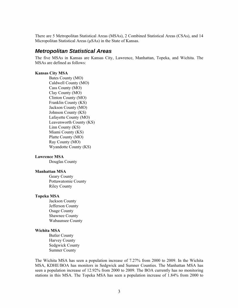
There are 5 Metropolitan Statistical Areas (MSAs), 2 Combined Statistical Areas (CSAs), and 14 Micropolitan Statistical Areas (μSAs) in the State of Kansas.

Metropolitan Statistical Areas The five MSAs in Kansas are Kansas City, Lawrence, Manhattan, Topeka, and Wichita. The MSAs are defined as follows: Kansas City MSA Bates County (MO) Caldwell County (MO) Cass County (MO) Clay County (MO) Clinton County (MO) Franklin County (KS) Jackson County (MO) Johnson County (KS) Lafayette County (MO) Leavenworth County (KS) Linn County (KS) Miami County (KS) Platte County (MO) Ray County (MO) Wyandotte County (KS) Lawrence MSA Douglas County Manhattan MSA Geary County Pottawatomie County Riley County Topeka MSA Jackson County Jefferson County Osage County Shawnee County Wabaunsee County Wichita MSA

Butler County Harvey County Sedgwick County Sumner County

The Wichita MSA has seen a population increase of 7.27% from 2000 to 2009. In the Wichita MSA, KDHE/BOA has monitors in Sedgwick and Sumner Counties. The Manhattan MSA has seen a population increase of 12.92% from 2000 to 2009. The BOA currently has no monitoring stations in this MSA. The Topeka MSA has seen a population increase of 1.84% from 2000 to

3

2009. The BOA has one monitoring site in Shawnee County. The Lawrence MSA has seen a population increase of 16.43% from 2000 to 2009. BOA currently does not have a monitoring site in Douglas County although an ozone monitor ran in this county from 2003 to 2006. The Kansas City MSA has seen a population increase of 12.61% from 2000 to 2009. In the Kansas City MSA, BOA has monitors in Leavenworth, Linn, Johnson and Wyandotte Counties. The U. S. Census Bureau 2000-2009 population change data of these MSAs is shown in Appendix B.

Combined Statistical Areas The two CSAs in Kansas are Kansas City-Overland Park-Kansas City and Wichita-Winfield. The CSAs are defined as follows: Kansas City-Overland Park-Kansas City CSA Kansas City, MO-KS MSA Warrensburg, MO μSA Atchison, KS μSA Wichita-Winfield CSA Wichita, KS MSA Winfield, KS μSA The Kansas City-Overland Park-Kansas City CSA has seen a population increase of 12.39% from 2000 to 2009. The KDHE/BOA operates 7 monitoring sites in this CSA. The Wichita-Winfield CSA has seen a population increase of 6.4% from 2000 to 2009. The BOA operates 7 monitoring sites in this CSA. The U. S. Census Bureau 2000-2009 population change data of these CSAs is also shown in Appendix B.

Micropolitan Statistical Areas KDHE operates monitors in three micropolitan statistical areas, Coffeyville, Dodge City and Salina. The fourteen μSAs in Kansas are defined as follows: Atchison μSA*** Atchison County Coffeyville μSA Montgomery County Dodge City μSA Ford County Emporia μSA*** Lyon County Chase County Garden City μSA*** Finney County Great Bend μSA*** Barton County

4

Hays μSA*** Ellis County Hutchinson μSA*** Reno County Liberal μSA*** Seward County McPherson μSA*** McPherson County Parsons μSA*** Labette County Pittsburg μSA*** Crawford County Salina μSA Ottawa County Saline County Winfield μSA*** Cowley County

*** The KDHE/BOA does not operate any monitors in these μSAs. The U. S. Census Bureau 2000-2009 population change data of these μSAs is shown in Appendix C.

Anticipated Growth/Decline According to the U. S. Census Bureau, the growth or decline of these 2 Combined Statistical Areas (CSAs), 5 Metropolitan Statistical Areas (MSAs), and 14 Micropolitan Statistical Areas (μSAs) is anticipated to maintain a similar trend over the next several years.

Kansas Criteria Pollutant Emissions Trends Emissions of criteria pollutants in Kansas continue to decrease as vehicles become cleaner and as facilities become more efficient and install controls. Table 1 below shows historic and recent criteria pollutant emissions (tons) in the EPA’s NEI database from 1990 to 2005. Emissions in the on-road mobile sector continue to decrease as tougher fleet emission standards and fuel requirements are implemented. Point source emissions have also decreased for most pollutants during this time period with major decreases in NOx emissions. Note that the methodology from period to period can change leading to large differences in reported values. For example, in 2002 the NH3 inventory in for Kansas included CAFO’s as point sources, thus the NH3 for point sources in this period was high while the nonpoint NH3 values were lower for this period. Another notable difference is the 1999 CO and NOx values for the nonpoint category which appears to be missing categories of emissions that were included in other years.

5

Table 1. Kansas Criteria Pollutant Emissions 1990-2005 (tons)

Year Source

Category CO NH3 NOx PM10 SO2 VOC

1990 Area (nonpoint) 341,392 197,231 57,346 833,353 2,643 147,8601996 Area (nonpoint) 1,015,045 215,345 94,767 843,128 4,286 255,4351999 Area (nonpoint) 95,372 225,729 15,055 751,195 3,530 97,7912002 Area (nonpoint) 843,535 113,057 41,836 720,047 36,182 132,0432005 Area (nonpoint) 897,771 168,761 49,411 754,205 39,384 181,981

1990 Nonroad mobile 240,177 646 78,152 7,892 5,874 26,353

1996 Nonroad mobile 271,023 602 87,449 7,906 7,445 28,283

1999 Nonroad mobile 265,984 59 85,328 7,376 7,765 25,006

2002 Nonroad mobile 268,920 35 82,129 7,994 7,050 24,229

2005 Nonroad mobile 220,441 45 86,691 5,986 8,081 24,702

1990 On-road mobile 1,288,874 1,713 112,697 4,671 6,037 103,9211996 On-road mobile 922,869 2,443 97,998 3,242 3,277 66,4511999 On-road mobile 768,862 2,727 93,125 2,696 3,439 58,5842002 On-road mobile 679,737 2,869 85,585 2,200 2,893 47,2512005 On-road mobile 538,060 3,021 68,176 1,915 1,824 43,8981990 Point 72,205 12,552 182,512 39,551 124,078 45,6791996 Point 81,757 12,593 195,309 14,632 131,192 26,5481999 Point 98,667 916 177,790 22,538 134,716 30,9942002 Point 81,234 52,681 165,586 17,038 140,619 27,187

2005 Point 35,397 1,813 157,984 11,166 146,997 26,106Source EPA National Emissions Inventory (NEI) Kansas conducts an annual point source inventory of permitted sources in the state. The inventory covers both permitted Title V facilities and those facilities that take a permit limit to avoid a Title V permit. Figure 1 below shows the trend in emissions from 1990 – 2008. Note PM2.5 is not included in the trend because this pollutant was not collected until recently. As one can see from the graph point source emissions have all trended down over the years. KDHE expects this trend to continue for all pollutants, especially for SOx, due to operation of scrubbers on electric generating units (EGU’s), and NOx, due to installation and operating of low NOx burners and selective catalytic reduction (SCR) at EGU’s.

6

Figure 1. Point Source Emissions Trends 1990-2008

Kansas Point Emissions 1990-2008

0

50,000

100,000

150,000

200,000

250,000

1990

1992

1994

1996

1998

2000

2002

2004

2006

2008

ton

s

NOx

SO2

PM10

VOC

CO

HAPs

NH3

Source KDHE KEI database

Current Criteria Emissions in Kansas Particle pollution is a general term used for a mixture of solid particles and liquid droplets found in the air. EPA regulates particle pollution as PM2.5 (fine particles) and PM10 (all particles 10 micrometers or less in diameter). The PM2.5 NAAQS was first introduced in 1997, thus trend data is not available for this pollutant for the entire period of 1990 – 2008. PM2.5 emission densities correlate closely with large facilities, populated areas, and areas in the Flint Hills where burning occurs. KDHE expects direct PM2.5 emissions to remain fairly consistent in the near term. Secondary formation of PM2.5 will likely continue to decrease as emissions of NOx and SOx continue to decrease. Generally the secondary PM2.5 will be formed in upwind counties (and states) and be transported downwind. This transport can occur from large distances. PM10 emissions densities track closely with population centers. This correlation includes both the residential and industrial processes as well as the mobile component. Much like PM2.5, KDHE anticipates PM10 emissions will remain fairly flat into the near future. Carbon monoxide (CO) is a colorless and odorless gas formed when carbon in fuel is not burned completely. CO emission densities track population centers very closely. Because CO is a function of fossil fuel combustion, the residential, commercial and industrial component along with the mobile portion drives the CO emissions. The large drop in CO emissions that occurred in 2004 can be attributed to Columbian Chemicals, a carbon black plant, which significantly decreased their CO emissions by installing a flare. KDHE anticipates CO emissions will remain fairly constant throughout the coming years.

7

Ground level ozone is the pollutant of concern that necessitates tracking emissions of nitrogen oxides (NOx) and volatile organic compounds (VOCs). Ozone forms when VOC and NOx react in the presence of sunlight. These ingredients come from motor vehicle exhaust, power plant and industrial emissions, gasoline vapors, chemical solvents, and from natural sources. Nitrogen dioxide (NO2) is a member of the nitrogen oxide (NOx) family of gases. It is formed in the air through the oxidation of nitric oxide (NO) emitted when fuel is burned at a high temperature. NOx emission densities are higher in counties with large EGU’s, numerous gas compressor stations or those counties with a large population. Kansas has several large power plants that made up a significant portion of the total NOx emissions in the state. Several of these power plants have or will be reducing their NOx emissions in the coming years. In the Kansas City area a recent NOx RACT rule went into place after contingency measures for ozone were triggered. These RACT rules will further decrease NOx emissions in this area. The trend line for NOx indicates a large reduction over the years with a significant downward slope in the recent years. KDHE expects additional NOx reductions exceeding 10,000 tons/yr as additional NOx controls are placed on Jeffrey energy center and other power plants within the state. VOC emissions densities are associated with both population centers and the Flint Hills area in Kansas where burning occurs. The overall trend in point source VOC emissions has been a decrease as various controls over the years have decreased these emissions. KDHE anticipates VOC emissions from the point sector will remain fairly flat over the coming years. VOC emissions associated with burning will vary from year to year as the amount burned varies from year to year. VOC is a precursor pollutant for ozone. Sulfur dioxide (SO2), a member of the sulfur oxide (SOx) family of gases, is formed from burning fuels containing sulfur (e.g., coal or oil) or from the oil refining process. SO2 dissolves in water vapor to form acid and can interact with NH3 and particles to form sulfates. SOx emissions densities reflect the location of the coal fired power plants within the state. Coal fired EGU’s and the states’ refineries are the largest sources of SOx emissions in Kansas. Similar to NOx emissions, the trend is downward for this pollutant. KDHE expects significant additional reductions in SOx over the next few years as scrubbers are installed and operated on the largest coal fired power plants within the state. There will be a significant decrease of SOx emission at Jeffrey energy center, the largest SOx emission source in the state, which should show up in the 2010 emission inventory. Ammonia (NH3) emissions densities in Kansas are most strongly associated with confined animal feeding operations and agriculture in general. NH3 is a precursor to secondary sulfate and nitrate particulate formation. KDHE anticipates NH3 emissions will remain fairly consistent over the next few years and will continue to remain strongly associated with agricultural related activities. Kansas has several large emissions sources that will be installing controls over the next few years. The controls are mainly associated with reducing NOx and SOx emissions. The controls are associated with the Regional Haze and other various control programs such as new MACT rules and consent decrees associated with EPA actions. KDHE will also continue to receive construction permits for major sources. The largest construction permit currently being processed by KDHE is associated with a coal burning power plant that will be located in Finney County in southwest Kansas. This will be a major source of emissions; however the facility will be very well controlled and is located far away from the major population centers within the state.

8

9

Appendix I contains emissions density (tons/miles2) plots on a county basis both for Kansas and the surrounding states. The emissions densities were calculated using the 2005 NEI emissions and include all anthropogenic emissions categories. Biogenic emissions are not included in these numbers. As one would expect emissions are generally higher in heavily populated counties or in counties that have large emitting facilities such as power plants. Appendix D contains the latest emission inventory for individual sources in the state and a map of all Title V and PSD permitted facility source locations in the state.

Ozone Monitoring Network

Current O3 Standard and Monitoring Requirements Current national ambient air quality standards (NAAQS) for O3 have been set to 0.075 parts per million (ppm) for both the primary standard and the secondary standard (http://www.epa.gov/fedrgstr/EPA-AIR/2008/March/Day-27/a5645.pdf). Based on the reconsideration of the current standard, EPA is proposing to strengthen the 8-hour “primary” ozone standard, designed to protect public health, to a level within the range of 0.060-0.070 parts per million (ppm) in the proposed rules published on January 19, 2010 (http://www.epa.gov/air/ozonepollution/fr/20100119.pdf). The proposed monitoring revisions would change minimum monitoring requirements in urban areas, add new minimum monitoring requirements in non-urban areas, and extend the length of the required ozone monitoring season specified as following (http://www.epa.gov/air/ozonepollution/pdfs/fs20100106std.pdf):

urban areas with populations between 50,000 and 350,000 people operate at least one ozone monitor.

states are required to operate at least three ozone monitors in non-urban areas. The new rule is expected to be finalized in October 2010, therefore the current network assessment for the upcoming 5 years must take the proposed rules into consideration. However, since the standard has not yet been announced or set, and the new monitoring requirements are not yet in effect, KDHE will take the proposals into consideration but will still rely upon the current monitoring standard and guidelines. Since monitoring data quality assurance reviews of the 2009 measurements have not yet been completed, monitoring data from 2004-2008 are used in this analysis.

State of Kansas Current O3 Monitoring Network Current Kansas O3 monitoring network includes 9 monitors located throughout the state. Monitors are listed in Table 2 along with detailed site information. No collocated O3 measurements are available in Kansas. Table 2. State of Kansas O3 Monitor Site ID and Location.

Site Name Site ID Latitude Longitude Address

Heritage Park 091 - 0010 38.83859 -94.74643 13899 W 159th (Heritage Park)

Leavenworth 103 - 0003 39.32746 -94.95127 2010 Metropolitan

Mine Creek 107 - 0002 38.13583 -94.731944 County Rd 1103 .7 Mi South Of K-52 (Mine Creek)

Park City 173 - 0001 37.78139 -97.337222 County Fire Station#2 ,200 East 53rd St.Nort

Wichita Health Dept. 173 - 0010 37.70111 -97.313889 Health Dept., 1900 East 9th St.

Topeka KNI 177 - 0013 39.02427 -95.71128 2501 Randolph Avenue

Peck 191 - 0002 37.47694 -97.366389 707 E 119th St South,Peck Community Bldg

10

http://www.epa.gov/fedrgstr/EPA-AIR/2008/March/Day-27/a5645.pdf

http://www.epa.gov/air/ozonepollution/fr/20100119.pdf

http://www.epa.gov/air/ozonepollution/pdfs/fs20100106std.pdf

Cedar Bluff 195 - 0001 38.77028 -99.763611 Cedar Bluff Reservoir, Pronghorn & Muley

Kansas City JFK 209 - 0021 39.1175 -94.635556 1210 N. 10th St.,JFK Recreation Center

Figure 2 showed the population density of the State of Kansas along with the monitoring sites (http://www.census.gov/popest/counties/tables/CO-EST2008-01-20.xls). Among these monitors, Topeka KNI, Peck and Kansas City JFK are urban scale monitors measuring population exposure; Park City is urban scale monitor measuring highest concentration; Heritage Park and Leavenworth are neighborhood scale monitors measuring population exposure; Mine Creek and Peck are regional scale monitors measuring regional transport; and Cedar Bluff is regional scale monitor measuring the general background O3 concentration in the state of Kansas. Figure 2. State of Kansas Population Density Map and the Location of O3 Monitors.

O3 Measurements Trend Analysis 30-day rolling averages of the daily maximum 8-hour O3 concentrations during 2004-2008 are presented in Figure 3 – Figure 5. Figure 3 included measurements from monitors within close proximity to Kansas City area. The monitor at Mine Creek is further away; however, measurements at this site were included due to the fact that measurements at Mine Creek were designed to represent regional transport into the Kansas City area.

11

http://www.census.gov/popest/counties/tables/CO-EST2008-01-20.xls

In general, O3 concentrations at all 4 monitors show similar magnitude of concentration and track each other fairly well during the entire 5-year period. High concentrations were observed in summer and low concentrations appear during the winter season as expected. Multiple spikes are observed during the ozone season (April 1 – October 31) each year; the spikes do not necessarily appear at the same time from year to year since summer ozone concentrations are also substantially affected by meteorological conditions (such as ambient temperature, cloud coverage, humidity and precipitation). However, each year the very first distinguishable peaks appear around April, with a high probability that significant contributions to these peeks are from the O3 formed by the annual burning activities occurring in the Flint Hills area approximately 120 miles west of Kansas City. The data does show that the measurements at Kansas City JFK site observed lower O3 concentration in winter in comparison with the other measurements nearby, especially in early 2008, possibly caused by the slower rate of O3 production in winter due to reduced insolation and low temperatures, combined with O3 consumption by NOx in urban center (Kansas City JFK) where NOx is readily available. Figure 3. 30-day Rolling Average of Daily Maximum 8-hour O3 Concentration at Monitors near Kansas City.

0

0.01

0.02

0.03

0.04

0.05

0.06

0.07

0.08

01/01/04

01/31/04

03/01/04

04/01/04

05/01/04

06/01/04

07/01/04

07/31/04

08/31/04

09/30/04

10/31/04

11/30/04

12/30/04

01/30/05

03/01/05

04/01/05

05/01/05

05/31/05

07/01/05

07/31/05

08/31/05

09/30/05

10/30/05

11/30/05

12/30/05

01/30/06

03/01/06

03/31/06

05/01/06

05/31/06

07/01/06

07/31/06

08/30/06

09/30/06

10/30/06

11/30/06

12/30/06

01/29/07

03/01/07

03/31/07

05/01/07

05/31/07

06/30/07

07/31/07

08/30/07

09/30/07

10/30/07

11/29/07

12/30/07

01/29/08

02/29/08

03/30/08

04/29/08

05/30/08

06/29/08

07/30/08

08/29/08

09/28/08

10/29/08

11/28/08

12/29/08

30‐Day Rolling Average of D

aily M

ax of 8

‐hr Conc

Date

Mine Creek Heritage Park Kansas City JFK Leavenworth

The 30-day rolling averages of the daily maximum 8-hour O3 concentrations near Wichita are presented in Figure 4. Wichita Health Department is the urban center site located in downtown Wichita; Peck monitor is located to the south of the Wichita Health Department monitor, measuring regional O3 transport into Wichita; and Park City monitor is located to the north of Wichita measuring O3 concentration after the air parcel travels through the city. Measurements from all three monitors show a consistent pattern: O3 concentrations are high in summer and low in winter. Normally highest O3 concentrations were measured at Peck as the air parcel coming into the city. They decreased slightly when arriving at the downtown Health Department site and drop further when reaching Park City monitors presumably due to the reaction with NOx inside the city of Wichita. Peck measurements between April 2004, and April,

12

2005 have been determined to be faulty, after reviewing the measurements patterns at all 3 sites for the past 10 years, plus including the measurements at a nearby Oklahoma site (400719010). The significant drop of Wichita Health Department measurements in late 2007 and early 2008 are likely due to the high ozone consumption by NOx with little O3 production, similar to those observed by the JFK Kansas City monitor during the same time period. There are discernable spikes starting around April each year. This likely indicates that the Flint Hills burning also affects the Wichita area. The April peaks in Wichita do not show the same pattern as those in Kansas City. This is because a different predominant wind direction determines the area which the burning affects. Kansas City and Wichita are in different directions with respect to the Flint Hills region; therefore, it is less likely that the O3 concentrations at both of these areas are significantly impacted by the burning activities at the same time. Figure 4. 30-day Rolling Average of Daily Maximum 8-hour O3 Concentration at Monitors near Wichita, KS.

0

0.01

0.02

0.03

0.04

0.05

0.06

0.07

0.08

01/01/04

01/31/04

03/01/04

04/01/04

05/01/04

06/01/04

07/01/04

07/31/04

08/31/04

09/30/04

10/31/04

11/30/04

12/30/04

01/30/05

03/01/05

04/01/05

05/01/05

05/31/05

07/01/05

07/31/05

08/31/05

09/30/05

10/30/05

11/30/05

12/30/05

01/30/06

03/01/06

03/31/06

05/01/06

05/31/06

07/01/06

07/31/06

08/30/06

09/30/06

10/30/06

11/30/06

12/30/06

01/29/07

03/01/07

03/31/07

05/01/07

05/31/07

06/30/07

07/31/07

08/30/07

09/30/07

10/30/07

11/29/07

12/30/07

01/29/08

02/29/08

03/30/08

04/29/08

05/30/08

06/29/08

07/30/08

08/29/08

09/28/08

10/29/08

11/28/08

12/29/08


aily M

ax of 8

‐hr Conc

Date

Peck Wichita Health Dept Park City

Measurements of the only other two Kansas O3 monitors are shown in Figure 5. Topeka/KNI site is a relatively new site and has only been operated since late 2006; it follows the trend of the other measurements. The Konza O3 measurements in Figure 4 were obtained from EPA’s Clean Air Status and Trends Network (CASTNET), where KDHE manually obtained the daily maximum of the 8-hr rolling average from the hourly data that are available (http://www.epa.gov/castnet/data.html). In general, all 3 measurements show seasonal pattern with high O3 concentrations observed in summer and low concentrations in winter. In fact, Konza measurements and Cedar Bluff measurements track each other very well with a high R2 value of 0.87 over the 5-year period. In most years, the April O3 concentration spikes are more prominent at the Konza site, since Konza site is located within the Flint Hills region while the Cedar Bluff site is further west. Another interesting observation is that although Cedar Bluff is chosen as the background site due to the fact that it is not near any significant emission sources, the 30-day rolling average of daily

13

http://www.epa.gov/castnet/data.html

maximum 8-hour O3 concentrations at Cedar Bluff are generally not any lower than most other ozone sites throughout the state of Kansas as shown in Figures 3-5. This indicates that the background O3 concentration in Kansas is fairly high, and it is likely that the actual contributions from local emissions on average are a fairly small contribution to the existing conditions at many Kansas ozone monitors. Local emissions do play a role in the urban areas, especially in the Kansas City metro area on peak ozone days. Figure 5. 30-day Rolling Average of Daily Maximum 8-hour O3 Concentration at Topeka/KNI, Cedar Bluff and Konza Prarie.

0

0.01

0.02

0.03

0.04

0.05

0.06

0.07

0.08

01/01/04

01/31/04

03/01/04

04/01/04

05/01/04

06/01/04

07/01/04

07/31/04

08/31/04

09/30/04

10/31/04

11/30/04

12/30/04

01/30/05

03/01/05

04/01/05

05/01/05

05/31/05

07/01/05

07/31/05

08/31/05

09/30/05

10/30/05

11/30/05

12/30/05

01/30/06

03/01/06

03/31/06

05/01/06

05/31/06

07/01/06

07/31/06

08/30/06

09/30/06

10/30/06

11/30/06

12/30/06

01/29/07

03/01/07

03/31/07

05/01/07

05/31/07

06/30/07

07/31/07

08/30/07

09/30/07

10/30/07

11/29/07

12/30/07

01/29/08

02/29/08

03/30/08

04/29/08

05/30/08

06/29/08

07/30/08

08/29/08

09/28/08

10/29/08

11/28/08

12/29/08


aily M

ax of 8

‐hr Conc

Date

Topeka KNI Cedar Bluff Konza

The design values for each O3 monitor during the last 5 years have been listed in Table 3. The values exceeding the current NAAQS for O3 are listed in bold italic font. A downward trend in O3 design values is observed at most sites. This trend would be more obvious if we include the design value for 2009 for each site. During the past 5 years, all sites in Kansas have no more than 1 year with O3 design value exceeding the NAAQS, except for Heritage Park, where 2 design values (non-consecutive years) exceed the standard. These data indicate none of the Kansas monitors show consistent exceedance of the current O3 standard; rather it is the special conditions or episodes that pushed the O3 concentration above the standard. It is important to note that meteorological conditions play a large part in producing ozone, thus a downward ozone trend does not necessarily indicate a reduction in the pre-cursor emissions that cause ozone. The downward trends could be a function of both favorable meteorological conditions and reductions in emissions.

14

Table 3. O3 Design Values for all Kansas Monitors during the Past 5 Years.

Site Name 02-04

Average 03-05

Average 04-06

Average 05-07

Average 06-08

Average

Heritage Park 0.076 0.074 0.076 0.069

Leavenworth 0.075 0.073 0.077 0.072

Mine Creek 0.072 0.073 0.073 0.074 0.070

Park City 0.069 0.066 0.063 0.062 0.060

Wichita Health Dept. 0.077 0.074 0.071 0.069 0.066

Topeka KNI

Peck 0.069 0.068 0.069 0.076 0.072

Cedar Bluff 0.070 0.069 0.072 0.071 0.069

Kansas City JFK 0.075 0.075 0.074 0.077 0.072

Correlations between Kansas O3 Monitors Figure 6 presents the correlation matrix adapted from the EPA statistic analysis tool (cormat.bat) for 2008 O3 measurements from May through September. The correlation matrix for year 2005, 2006, and 2007 are included in Appendix F. Similar to the tool provided by EPA, the shape of the ellipses represents the Pearson squared correlation between sites with circles representing zero correlation and straight diagonal line representing a perfect correlation. The color of the ellipses represents the average difference between sites. The number in black inside each circle represents the distance between the corresponding sites. The difference between Figure 6 and the figures from the original EPA tool are the correlation coefficients that have been added inside each circle (in blue), and the color scale of the average relative difference has been modified in order to better emphasize the average relative differences which are generally below 0.3 for ozone. Therefore, although we see colors ranging from light yellow to red, none of the following pairings has relative difference of more than 0.3.

15

Figure 6. Correlation Matrix for 2008 O3 Measurements in Kansas.

In general, good correlations were observed for the Kansas City monitoring sites. Among the four monitoring sites near Kansas City, Heritage Park (200910010) shows very high correlation and low relative difference compared to the other 3 sites. Therefore measurements at Heritage Park are good representations of the entire Kansas City region. On the other hand, Mine Creek (201070002) is a regional transport site; therefore it only exhibits high correlation with Heritage Park, which is the first monitoring site that the air shed passes by after it leaves Mine Creek traveling toward the Kansas City area. The correlations between Mine Creek and JFK (202090021) or Leavenworth (201030003) are not as good, since JFK represents urban center atmosphere with additional ozone production or consumption reactions, and Leavenworth being even further away from JFK and subject to additional urban core emissions. The relative difference of Mine Creek with the other three Kansas City sites shows an opposite trend as the correlations, with lowest relative difference between Mine Creek and Heritage Park, and higher between Mine Creek and Leavenworth or JFK. Topeka/KNI is an urban site not too far away (50 miles west) from the Kansas City urban center sites; this site generally tracks very well with the three Kansas City sites (high correlation and low relative difference). Topeka/KNI site does not track as well to the Mine Creek site for similar reasons stated above.

16

All three Wichita sites also show high correlation among each other. These three sites are located within 35 miles of each other. Based on the correlation and the relative close distance it seems feasible that one of the Wichita sites (Park City) could be relocated, possibly further downwind of the urban core. The correlations between Wichita sites and Kansas City sites are generally not very good since the monitoring sites are quite far away and are influenced by different factors most of the time.

Removal Bias Analysis In the EPA network assessment toolkit a removal bias utility was included. The removal bias tool provides an average bias, of removing a monitor. This average bias is calculated by performing a Voronoi neighborhood averaging algorithm with and without a monitor and taking the difference. A positive average bias would mean that if the site being examined was removed, the neighboring sites would indicate that the estimated concentration would be larger than the measured concentration. Likewise, a negative average bias would suggest that the estimated concentration at the location of the site is smaller than the actual measured concentration. So, those sites with large positive bias are more likely candidates to be removed or relocated because they are not measuring the peak ozone in the area. Figure 7 shows the results of this removal bias tool run in the Wichita area. Red circles indicate positive bias while blue indicate negative bias. The average bias for the Peck, 201910002, is -0.001 ppm indicating the removal of this site would cause the average using the remaining sites to be lower than this site is reading. So this site is not a good candidate to remove. Likewise Park City has a removal bias of 0.006 ppm which indicates the removal of this site would make the average of the remaining sites increase. This indicates that this site may be a good candidate to remove or relocate to a location that may have higher ozone readings. Based on the orientation of the monitors in Wichita and the predominant wind direction during the summertime ozone season and this removal bias result, the Park City monitor should likely be moved further downwind of the metro area to attempt to pick up peak ozone readings caused from local precursor emissions. It appears that the Park City monitor is experiencing NOx titration and thus ozone is being depressed at this monitor from the local NOx emissions from the urban core. Moving this monitor further downwind would not impact the design value of the area. A monitor further downwind would also likely start picking up the ozone formed from the locally generated precursor emissions.

17

Figure 7. Removal Bias Run for 201730001, 101730010 and 201910002

Proposed O3 Monitoring Requirements Based on the requirements of the proposed monitoring rules published in January, 2010, EPA proposed that Metropolitan Statistical Areas (MSA) with populations ranging from 50,000 to less than 350,000 should have at least one O3 monitor in place. Kansas MSA’s that fall within this range include Wichita, Kansas City, Topeka and Lawrence. Of these four MSA’s only Lawrence does not currently have an O3 monitor. Based on this proposed guidance, KDHE intends on placing an ozone monitor in the Lawrence MSA in the next 5 years. In addition to the new guidance for MSA monitoring there is also guidance for non-urban areas. The guidance states that each state should have a minimum of 3 non-urban sites. These non-urban sites are intended to meet the following objectives:

18

(1) To provide characterization of O3 exposures to O3-sensitive vegetation and important ecosystems, at least one monitoring site is to be located in an area such as those set aside to conserve the scenic value and the natural vegetation and wildlife within such areas.

(2) To provide O3 characterization of less-populated areas, at least one monitoring site is to be located to represent a Micropolitan Statistical Area expected to have a maximum O3 design value concentration of at least 85 percent of the NAAQS.

(3) To provide O3 characterization in non-urban areas impacted by transport, at least one monitoring site is to be located in the area of expected maximum O3 concentration outside of currently monitored MSAs, Micropolitan Statistical Areas, and sensitive ecosystems.

KDHE has evaluated this proposed guidance and believes the current Cedar Bluff monitor meets the intent of objective (1) above. The Cedar Bluff monitor is located in a state park in an area with nearby ozone sensitive agricultural vegetation along with natural vegetation and wildlife located within the park itself. For objective (2) above, KDHE evaluated Micropolitan Statistical Areas within the state. Based on the census bureau’s projections for Kansas population in the year 2008, Manhattan, Hutchinson, and Salina are the largest Micropolitan Statistical Areas not currently monitored for O3 (http://www.census.gov/popest/metro/CBSA-est2008-annual.html). Table 4 listed all Kansas MSAs and Micropolitan Statistical Areas (in Italic) based on the current census definitions, with their populations and O3 monitoring activities (http://www.census.gov/popest/metro/tables/2008/CBSA-EST2008-01.xls). Based on this, KDHE proposes a Salina area O3 monitor to meet objective (2). Salina is downwind of Wichita (a major metropolitan area) and would be expected to potentially see transport of precursor emissions and ozone from the Wichita area. For objective (3) above KDHE believes the Mine Creek monitor meets these criteria. Note that KDHE is proposing to move the Mine Creek monitor to the Chanute area towards the end of the 5 year review period. This new location should also meet the intent of objective (3) above. Table 4. Populations and O3 Monitoring Activities for Current Kansas MSAs.

MSA Population

(07/08/2008) Existing O3 Monitors

New O3 Monitors Required

Wichita, KS 603,716 Y N Topeka, KS 229,619 Y N Lawrence, KS 114,748 N Y Manhattan, KS 121,935 N N Hutchinson, KS 63,427 N N Salina, KS 60,683 N N Kansas City, MO-KS 2,002,047 Y N St. Joseph, MO-KS 126,359 Y N

Proposed Kansas O3 Monitoring Networks for the Upcoming 5 Years After a careful review of all the above factors, the proposed Kansas O3 monitoring network for the upcoming 5 years is presented in Figure 8. This proposal reflects the newly proposed population based and non-urban monitoring requirements that come with the newly proposed ozone standard along with the relocation of the Park City monitor further downwind of Wichita in

19

http://www.census.gov/popest/metro/CBSA-est2008-annual.html

http://www.census.gov/popest/metro/tables/2008/CBSA-EST2008-01.xls

order to pick up peak ozone caused from local precursor emissions and a relocation of Mine Creek to Chanute to better cover the South East portion of the state while still providing upwind ozone values for Kansas City. Overall, KDHE proposes adding three new ozone monitors in Lawrence, Salina, and Garden City and relocating two monitors Park City to Newton, KS and Mine Creek to Chanute KS. Figure 8. Proposed O3 Monitoring Network for the State of Kansas for the Upcoming 5 Years

PM2.5 Monitoring Network

Current PM2.5 Standard and Monitoring Requirements Current national ambient air quality standards (NAAQS) for PM2.5 have been set to 15 micrograms per meter cubed annual average and 35 micrograms per meter cubed 24-hour average for both the primary standard and the secondary standard (http://www.epa.gov/ttn/naaqs/standards/pm/data/fr20061017.pdf). The annual standard is based on a 3 year average of the weighted annual mean. The 24-hour standard is based on a 3 year 98th percentile average of 24-hour values. Current minimum monitoring requirements for PM2.5 are shown in Table 5 (http://edocket.access.gpo.gov/2006/pdf/06-8478.pdf).

20

http://www.epa.gov/ttn/naaqs/standards/pm/data/fr20061017.pdf

http://edocket.access.gpo.gov/2006/pdf/06-8478.pdf

Table 5. PM2.5 Minimum Monitoring Requirements (Number Of Stations per MSA)

Population Category 3-yr design value > 85% of NAAQS

3-yr design value < 85% of NAAQS

> 1,000,000 3 2 500,000 - 1,000,000 2 1 50,000 - <500,000 1 0

In addition to the minimum number of monitors required, there are also requirements for a minimum number of continuous monitors to be deployed. Fifty percent of the minimum required number of monitoring sites are required to be a continuous PM2.5 monitor. For Kansas this means that at a minimum two continuous PM2.5 monitors need to be operated in the state. Applying the minimum monitoring requirements to Kansas urban areas, population totals and historical PM2.5 measurements results in the design requirements shown in Table 6. According to Tables 5 and 6, PM2.5 monitors could be removed from the Wichita area and the Kansas City area assuming the Missouri side of Kansas City retains a PM2.5 monitor(s). Table 6. Minimum Number of PM10 Monitors Required in Kansas MSA

MSA Population

(07/08/2008) Number of Existing

PM2.5 Monitors PM2.5 Monitors

Required Wichita, KS 603,716 3 1

Topeka, KS 229,619 1 0 Lawrence, KS 114,748 0 0 Kansas City, MO-KS 2,002,047 4 (KS side only) 2

State of Kansas Current PM2.5 Monitoring Network Current Kansas PM2.5 monitoring network includes 13 monitors located throughout the state at 11 different monitoring sites. Ten of the monitors are filter based while the remaining three monitors are continuous Tapered Element Oscillating Microbalance (TEOM). Only one of the TEOM monitors, located at JFK, is equipped with a Filter Dynamics Measurement System (FDMS) and is considered a federal reference monitor. Monitor locations and type are listed in Table 7 along with detailed site information. Two sites have collocated filterable and continuous PM2.5 measurements, one at JFK in Kansas City and one at Mine Creek south of Kansas City. Table 7. State of Kansas PM2.5 Monitor Site ID and Location.

Site Name Site ID City Address Lat_DD Lon_DD PM2.5 CPM2.5

Cedar Bluff 195 - 0001

Cedar Bluff

Cedar Bluff Reservoir,Pronghorn & Muley 38.77028 -99.7636 NO YES

Justice Center

091 - 0007

Overland Park 85th And Antioch 38.97444 -94.6869 YES NO

Heritage Park

091 - 0010 Olathe

13899 W 159th (Heritage Park) 38.83859 -94.7464 YES NO

Washington & Skinner

173 - 0008 Wichita

Fire Sta#11, G.Washington Blvd & E.Skinner 37.65972 -97.2972 YES NO

21

Glenn & Pawnee

173 - 0009 Wichita

Fire Sta#12 Glenn & Pawnee 37.65111 -97.3622 YES NO

Health Dept. 173 - 0010 Wichita

Health Dept., 1900 East 9th St. 37.70111 -97.3139 YES NO

KNI 177 - 0013 Topeka 2501 Randolph Avenue 39.02427 -95.7113 YES NO

Peck 191 - 0002 Peck

707 E 119th St South,Peck Community Bldg 37.47694 -97.3664 YES NO

Midland 209 - 0022

Kansas City

3101 S. 51st, Midland Trail Elem. School 39.04583 -94.6944 YES NO

Mine Creek 107 - 0002

Mine Creek

County Rd 1103 .7 Mi South Of K-52 (Mine Creek) 38.13583 -94.7319 YES YES

JFK 209 - 0021

Kansas City

1210 N. 10th St.,JFK Recreation Center 39.1175 -94.6356 YES YES

Figure 9 shows the population density of the State of Kansas along with the PM2.5 monitoring sites (http://www.census.gov/popest/counties/tables/CO-EST2008-01-20.xls). All of these monitors have 3 year design values below the 85% of the NAAQS concentration category. Figure 9. State of Kansas Population Density Map and the Location of PM2.5 Monitors.

PM2.5 Measurements Trend Analysis Both the continuous TEOM and filter based PM2.5 measurements were evaluated for trend analysis. Figure 10 displays the 24 hour data for the one-in-three monitoring for the ten filter based monitors. Note this graph shows 13 monitors, however, during the period the Shawnee County monitor was moved and for a short period was co-located, thus the three monitors in county 177 are now represented by KNI. Also, there was an additional monitor in Johnson

22


County, 091-0009, that operated only during 2006 which has also been included below. For the filter based monitoring the average trend across all filter based monitors is slightly downward. Figure 10. 24-hour Filter Based Monitoring Data Sites with Trendline 2004-2008.

0

5

10

15

20

25

30

35

40

45

50

2004

0101

2004

0301

2004

0430

2004

0621

2004

0810

2004

0920

2004

1117

2005

0116

2005

0317

2005

0516

2005

0715

2005

0913

2005

1112

2006

0111

2006

0312

2006

0505

2006

0704

2006

0824

2006

1020

2006

1216

2007

0211

2007

0412

2007

0611

2007

0810

2007

1009

2007

1208

2008

0203

2008

0403

2008

0602

2008

0801

2008

0930

2008

1129

date

ug

/m3

average

091-0007

091-0009

091-0010

107-0002

173-0008

173-0009

173-0010

177-0010

177-0011

177-0013

191-0002

209-0021

209-0022

Linear (average)

For the continuous data the trend over the 5-year period, 2004-2008, has been slightly upward. Figure 11 shows the 24-hour average of the three continuous monitors along with the linear trendline. It appears that the main reason for the upward trend in the continuous monitoring is the addition of the JFK monitor in 2007. This monitor is located in the Kansas City urban area and raises the overall average because it has slightly higher readings on average than the other two monitors. Overall, the average continuous and filterable PM2.5 readings across the state are below the NAAQS standard. Figure 11. 24-hr Average Continuous Monitoring Data with Trendline 2004-2008

0

5

10

15

20

25

30

35

40

45

50

200

40101

200

40321

200

40609

200

40828

200

41116

200

50204

200

50425

200

50714

200

51002

200

51221

200

60311

200

60530

200

60818

200

61106

200

70125

200

70415

200

70704

200

70922

200

71211

200

80229

200

80519

200

80807

200

81026

date

ug/m

3

average

107-0002

195-0001

209-0021

Linear (average)

23

Very similar trends are seen when looking at the annual averages. Figure 12 provides the annual average filter based PM2.5 readings from 2004 – 2008. As is seen in the 24-hr case the trend is slightly downward. Figure 12. Annual Average Filter Based Data 2004-2008

0

1

2

3

4

5

6

7

8

9

10

11

12

13

14

15

2004 2005 2006 2007 2008

Year

ug/m

3

091-0007

091-0009

091-0010

107-0002

173-0008

173-0009

173-0010

177-0010

177-0011

177-0013

191-0002

209-0021

209-0022

The design values for each PM2.5 monitor have been listed in Tables 8 and 9. There are no values exceeding the current NAAQS for PM2.5 annual or 24-hour standards. All federal reference monitors are also below 85% NAAQS threshold used for determining minimum monitoring requirements. The JFK TEOM-FDMS monitor is above this 85% threshold, however, this monitor does not have 3 years of data collection as a federal reference monitor with the FDMS installed. None of the three TEOM monitors had FRM equivalency for the 06-08 period. The TEOM monitors are listed in Italic in Tables 8 and 9 below. Table 8. 24-hour PM2.5 Design Values (98th percentile) for all Kansas Monitors (ug/m3).

Site Name 06-08

Average

Heritage Park 20

Cedar Bluff (TEOM) 17

Mine Creek 21

Mine Creek (TEOM) 24

Wichita Health Dept. 21

Pawnee & Glenn 22

Washinton & Skinner 21

Topeka KNI 23

Peck 21

24

Kansas City JFK (TEOM-FDMS)

29

Kansas City JFK 23

Justice Center 21

Midland 22 Table 9. Annual PM2.5 Design Values for all Kansas Monitors (ug/m3).

Site Name 06-08

Average

Heritage Park 9.0

Cedar Bluff (TEOM) 7.3

Mine Creek 10.1

Mine Creek (TEOM) 10.7

Wichita Health Dept. 9.5

Pawnee & Glenn 9.3

Washinton & Skinner 9.5

Topeka KNI 10.3

Peck 9.0 Kansas City JFK (TEOM-FDMS)

13.8

Kansas City JFK 11.1

Justice Center 9.7

Midland 10.0

Correlations between Kansas PM2.5 Monitors Figure 13 presents the correlation matrix from the EPA statistic analysis tool (cormat.bat) for 2008 PM2.5 measurements. The correlation matrix for year 2005, 2006, and 2007 are included in Appendix G. The shape of the ellipses represents the Pearson squared correlation between sites with circles representing zero correlation and straight diagonal line representing a perfect correlation. The color of the ellipses represents the average difference between sites. The number inside each circle represents the distance between the corresponding sites.

25

Figure 13. Correlation Matrix for 2008 PM2.5 Measurements in Kansas.

Very good correlations were observed for the Kansas City monitoring sites. Among the four monitoring sites in Kansas City on the Kansas side all these sites showed a >0.8 R2 correlation and low relative difference. Similar high correlations are seen in the other years. These four sites are also fairly well correlated with the Kansas City Missouri monitors. Based on the correlations two of these two monitors could likely be removed. All four of the Wichita sites also show very high (> 0.8 R2) correlation among each other. All four sites are located within 25 miles of each other. Note that not all monitors are included in the correlation tool based on data availability. Based on the correlation and the relative close distance between all sites it seems feasible that two or even three of the Wichita PM2.5 sites could be removed. Topeka/KNI is an urban site not too far away (50 miles west) from the Kansas City urban center sites; this site does not show a correlation with the three Kansas City sites. The remaining sites are also further distances from the urban core and generally are not correlated because of the large

26

distances between locations. Even though the correlations are low, most of these sites have similar low design values all below the NAAQS for both the annual and 24-hour standard.

Removal Bias Analysis In the EPA network assessment toolkit a removal bias utility was included. The removal bias tool provides an average bias, of removing a monitor. This average bias is calculated by performing a Voronoi neighborhood averaging algorithm with and without a monitor and taking the difference. A positive average bias would mean that if the site being examined was removed, the neighboring sites would indicate that the estimated concentration would be larger than the measured concentration. Likewise, a negative average bias would suggest that the estimated concentration at the location of the site is smaller than the actual measured concentration. So, those sites with large positive bias are more likely candidates to be removed or relocated because they are not measuring the peak PM2.5 in the area. Figure 14 shows the results of this removal bias tool run for PM2.5 sites in Kansas. Red circles indicate positive bias while blue indicate negative bias. Overall all Kansas filter based sites have a positive bias. Figure 14. Removal Bias Results for Kansas.

27

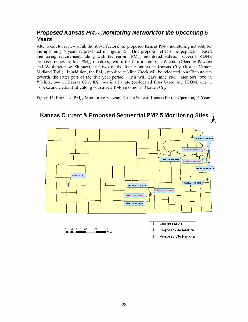
Proposed Kansas PM2.5 Monitoring Network for the Upcoming 5 Years After a careful review of all the above factors, the proposed Kansas PM2.5 monitoring network for the upcoming 5 years is presented in Figure 15. This proposal reflects the population based monitoring requirements along with the current PM2.5 monitored values. Overall, KDHE proposes removing four PM2.5 monitors, two of the four monitors in Wichita (Glenn & Pawnee and Washington & Skinner), and two of the four monitors in Kansas City (Justice Center, Midland Trail). In addition, the PM2.5 monitor at Mine Creek will be relocated to a Chanute site towards the latter part of the five year period. This will leave nine PM2.5 monitors, two in Wichita, two in Kansas City, KS, two in Chanute (co-located filter based and TEOM, one in Topeka and Cedar Bluff, along with a new PM2.5 monitor in Garden City. Figure 15. Proposed PM2.5 Monitoring Network for the State of Kansas for the Upcoming 5 Years

28

PM10 Monitoring Network

Current PM10 Standard and Monitoring Requirements Current national ambient air quality standards (NAAQS) for PM10 has been set to 150 micrograms per meter cubed for both the primary standard and the secondary standard (http://www.epa.gov/ttn/naaqs/standards/pm/data/fr20061017.pdf). This standard is not to be exceeded more than once per year on average over 3 years. Current minimum monitoring requirements for PM10 are shown in Table 10 (http://edocket.access.gpo.gov/2006/pdf/06-8478.pdf). Table 10. PM10 Minimum Monitoring Requirements (Number Of Stations per MSA)1

Population Category

High Concentration2

Medium Concentration3

Low Concentration4

> 1,000,000 6 - 10 4 - 8 2 - 4 500,000 - 1,000,000 4 - 8 2 - 4 1 - 2

250,000 - 500,000 3 - 4 1 - 2 0 - 1 100,000 - 250,000 1 -2 0 - 1 0

1 Selection of urban areas and actual numbers of stations per area within the ranges shown in this table will be jointly determined by EPA and the State Agency. 2 High concentration areas are those for which ambient PM10 data show ambient concentrations exceeding the PM10 NAAQS by 20% or more. 3 Medium concentration areas are those for which ambient PM10 data show ambient concentrations exceeding 80% of the PM10 NAAQS. 4 Low concentration areas are those for which ambient PM10 data show ambient concentrations < 80% of the PM10 NAAQS. 5 These minimum monitoring requirements apply in the absence of a design value. Applying the minimum monitoring requirements to Kansas urban areas, population totals and historical PM10 measurements results in the design requirements shown in Table 11. According to Tables 10 and 11, PM10 monitors could be removed from the Wichita area and the Kansas City area assuming the Missouri side of Kansas City retains a PM10 monitor. Table 11. Minimum Number of PM10 Monitors Required in Kansas MSA

MSA Population

(07/08/2008) Number of Existing

PM10 Monitors PM10 Monitors

Required Wichita, KS 603,716 4 1 – 2 Topeka, KS 229,619 1 0 – 1 Lawrence, KS 114,748 0 0 Kansas City, MO-KS 2,002,047 2 (KS side only) 2 – 4

State of Kansas Current PM10 Monitoring Network Current Kansas PM10 monitoring network includes 13 monitors located throughout the state at 11 monitoring sites. Six of the monitors are filter based while the remaining seven monitors are

29

http://www.epa.gov/ttn/naaqs/standards/pm/data/fr20061017.pdf



continuous. Monitor locations and type are listed in Table 12 along with detailed site information. Two sites have collocated filterable and continuous PM10 measurements, one in Topeka and one in Wichita. Table 12. State of Kansas PM10 Monitor Site ID and Location.

Site Name Site ID City Address Lat_DD Lon_DD PM10 Cont. PM10

Dodge City 057 - 0002 Dodge City Dodge City Community College 37.77527 -100.035 NO YES

Coffeyville 125 - 0006 Coffeyville Union & E. North /Ne Corner Intersection 37.046944 -95.613333 NO YES

Washington & Skinner 173 - 0008 Wichita

Fire Sta#11, G.Washingtonblvd & E.Skinne 37.659722 -97.297222 NO YES

Glen & Pawnee 173 - 0009 Wichita Fire Sta#12 Glen & Pawnee 37.651111 -97.362222 NO YES

Health Dept 173 - 0010 Wichita Health Dept., 1900 East 9th St. 37.701111 -97.313889 NO YES

Chanute 133 - 0002 Chanute 1500 West Seventh 37.676111 -95.474444 YES NO

Goodland 181 - 0001 Goodland City Fire Sta , 1010 Center 39.348333 -101.713056 YES NO

420 Kansas 209 - 0015 Kansas City Fire Sta#3 ,420 Kansas Ave 39.087778 -94.621389 YES NO

JFK 209 - 0021 Kansas City 1210 N. 10th St.,JFK Recreation Center 39.1175 -94.635556 YES NO

K-96 And Hydraulic 173 - 1012 Wichita K-96 And Hydraulic 37.747222 -97.316389 YES YES

KNI 177 - 0013 Topeka 2501 Randolph Avenue 39.02427 -95.71128 YES YES

Figure 16 shows the population density of the State of Kansas along with the monitoring sites (http://www.census.gov/popest/counties/tables/CO-EST2008-01-20.xls). All of these monitors have 3 year design values in the Low (< 80% of the NAAQS) concentration category.

30


Figure 16. State of Kansas Population Density Map and the Location of PM10 Monitors.

PM10 Measurements Trend Analysis Both the continuous TEOM and filter based PM10 measurements were evaluated for trend analysis. For the continuous data the trend over the 5-year period, 2004-2008, has been slightly upward. Figure 17 shows the daily average of the five continuous monitors along with the linear trendline. Overall, the average continuous readings across the state are well below the NAAQS standard even with a slight upward trend. Figure 17. Daily Average of all Continuous Monitoring Data Sites with Trendline 2004-2008.

0

10

20

30

40

50

60

70

80

20

04

01

01

20

04

03

12

20

04

05

22

20

04

08

01

20

04

10

11

20

04

12

21

20

05

03

02

20

05

05

12

20

05

07

22

20

05

10

01

20

05

12

11

20

06

02

20

20

06

05

02

20

06

07

12

20

06

09

21

20

06

12

01

20

07

02

10

20

07

04

22

20

07

07

02

20

07

09

11

20

07

11

21

20

08

01

31

20

08

04

11

20

08

06

21

20

08

08

31

20

08

11

10

Date

ug

/m3

31

Looking at the filter based one-in-six data, the upward trend is slightly higher than it was for the continuous data. This difference appears to be due to the data seen in the last quarter of 2008. Figure 18 shows the PM10 filter based monitoring data for PM10 sites in the state. Note the higher readings that occurred in the last quarter in 2008. This increase appears to be associated with both meteorological conditions and the monitoring frequency. For example, in December 2008 all five monitoring days occurred on days with a frontal passage that was coupled with high winds. So, it appears it was a coincidence that during the one-in-six monitoring in the latter part of 2008 was associated with generally windy conditions and the in-between days would have likely had lower PM10 readings had there been daily sampling. In fact you can see this trend in the continuous data for this period. Because of the coincidental meteorological conditions on the monitoring days KDHE believes the trend from one-in-six monitoring is not as representative as the trend from the continuous monitoring. The important point is both the continuous and filter based monitors are all well below the standard. Figure 18. Filter Based One-in-Six Monitoring Data 2004-2008

0

20

40

60

80

100

120

2004

0104

2004

0415

2004

0801

2004

1117

2005

0227

2005

0615

2005

0925

2006

0111

2006

0429

2006

0815

2006

1119

2007

0307

2007

0623

2007

1009

2008

0125

2008

0512

2008

0828

2008

1214

date

ug

/m3

057-0001

177-0010

177-0013

181-0001

209-0015

209-0021

The design values for each of the PM10 monitors have been listed in Table 13. There are no values exceeding the current NAAQS. The Kansas City monitor, 420 Kansas, has the highest design value at 88 ug/m3 which is well below the 150 ug/m3 standard. Several monitors do not have three years of data and no design values are provided for those monitors. Table 13. PM10 Design Values for all Kansas Monitors (ug/m3).

Site Name 2006 2nd

High 2007 2nd

High 2008 2nd

High

06-08 Design Value

Chanute 47 84 72 68

32

Goodland 37 45 66 49 KCK JFK 73 52 85 70 KCK 420 Kansas 84 76 103 88 Wichita Health Dept. 58 58 80 65 Topeka KNI 42 91 n/a Dodge City (TEOM) 94 n/a Coffeyville (TEOM) 57 90 51 66 Washington & Skinner (TEOM)

52 48 61 54

Glen & Pawnee (TEOM)

80 56 61 66

Wichita Health Dept (TEOM)

69 53 61 61

K96 & Hydraulic (TEOM)

67 54 61 61

Topeka KNI (TEOM) 47 49 n/a

Correlations between Kansas PM10 Monitors Figure 19 presents the correlation matrix from the EPA statistic analysis tool (cormat.bat) for 2008 PM10 measurements. The correlation matrix for year 2005, 2006, and 2007 are included in Appendix H. The shape of the ellipses represents the Pearson squared correlation between sites with circles representing zero correlation and straight diagonal line representing a perfect correlation. The color of the ellipses represents the average difference between sites. The number inside each circle represents the distance between the corresponding sites.

33

Figure 19. Correlation Matrix for 2008 PM10 Measurements in Kansas.

In general, good correlations were observed for the Kansas City monitoring sites. Among the two monitoring sites in Kansas City on the Kansas Side, 420 Kansas (202090015) and JFK (202090021), these sites showed a >0.6 R2 correlation and low relative difference. Similar high correlations are seen in the other years also. These two sites were not as well correlated with the Kansas City Missouri monitors. Based on the correlations one of these two monitors could likely be removed. Three of the four Wichita sites also show very high (> 0.85 R2) correlation among each other. All four sites are located within 11 miles of each other. The northern site (201731012) at K96 and Hydraulic is the outlier of the four with poor correlations between the remaining three sites. This site is likely being influenced by a local source since it has a much higher design value than the other three sites. Based on the correlation and the relative close distance between all sites it seems feasible that two or even three of the Wichita PM10 sites could be removed. The correlations between Wichita

34

sites and other sites are generally not very good since the monitoring sites are quite far away and outside of the urban core. Topeka/KNI is an urban site not too far away (50 miles west) from the Kansas City urban center sites; this site does not show a correlation with the three Kansas City sites. The remaining sites are in smaller cities such as Goodland, Coffeyville, Chanute and Dodge City. None of these sites are well correlated likely because of the large distances between locations. Even though the correlations are low, most of these sites have similar low design values. The exception is Chanute which has a design value of 121 ug/m3, which while higher than the other monitors, is still well below the standard.

Removal Bias Analysis In the EPA network assessment toolkit a removal bias utility was included. The removal bias tool provides an average bias, of removing a monitor. This average bias is calculated by performing a Voronoi neighborhood averaging algorithm with and without a monitor and taking the difference. A positive average bias would mean that if the site being examined was removed, the neighboring sites would indicate that the estimated concentration would be larger than the measured concentration. Likewise, a negative average bias would suggest that the estimated concentration at the location of the site is smaller than the actual measured concentration. So, those sites with large positive bias are more likely candidates to be removed or relocated because they are not measuring the peak PM10 in the area. Figure 20 shows the results of this removal bias tool run for PM10 sites in Kansas. Red circles indicate positive bias while blue indicate negative bias. Overall most Kansas sites have a positive bias. Although the Kansas City sites both have a negative bias, these two sites correlate closely. Of the remaining sites, K96 & Hydraulic in Wichita has a negative bias along with Chanute. Neither of these sites is being proposed for removal.

35

Figure 20. Removal Bias Results for Kansas.

Proposed Kansas PM10 Monitoring Network for the Upcoming 5 Years After a careful review of all the above factors, the proposed Kansas PM10 monitoring network for the upcoming 5 years is presented in Figure 21. This proposal reflects the population based monitoring requirements along with the current PM10 monitored values. Overall, KDHE proposes removing PM10 monitors in Goodland, Dodge City, two of the four monitors in Wichita (Glenn & Pawnee and Washington & Skinner), and one of the two monitors in Kansas City. This will leave five PM10 monitors, two in Wichita and one in Kansas City, KS, Coffeyville, Chanute and Topeka, along with a new monitor in Garden City.

36

Figure 21. Proposed PM10 Monitoring Network for the State of Kansas for the Upcoming 5 Years

State of Kansas NCore Monitoring Plan

National Ambient Air Monitoring Strategy The Environmental Protection Agency (EPA) has developed a new National Ambient Air Monitoring Strategy (NAAMS). The goal of the new strategy is “to improve the scientific and technical competency of existing air monitoring networks to be more responsive to the public, and the scientific and health communities, in a flexible way that accommodates future needs in an optimized resource-constrained environment” (National Ambient Air Monitoring Strategy Document). As part of the Strategy, a new network design has been proposed called the National Core Network (NCore). This network will accommodate the overall strategic goals as well as determine air quality trends, report to the public, assess emission reduction strategy effectiveness, provide data for health assessments and help determine attainment / non-attainment status. NCore introduces a new multi-pollutant monitoring component, and addresses the following major objectives: • Provide timely reporting of data to public through the AIRNow Web site (www.airnow.gov), air quality forecasting and other public reporting mechanisms; • Support the development of emission strategies through air quality model

37

evaluation and other observational methods; • Provide accountability of emission strategy progress through tracking long-term trends of criteria and non-criteria pollutants and their precursors; • Support long-term health assessments that contribute to ongoing review of National Ambient Air Quality Standards (NAAQS); • Evaluate compliance with NAAQS through designation of attainment / non-attainment areas; and • Support scientific studies ranging across technological, health, and atmospheric process disciplines. The Kansas Department of Health and Environment (KDHE) ambient air quality monitoring program has already accomplished much of the network reconfiguration needed to meet NCore objectives. Since 1999, as a result of implementing a major network reconfiguration associated with promulgation of the National Ambient Air Quality Standard (NAAQS) for PM2.5, the State of Kansas has:

1) completed a primary disinvestment in PM10 sampling;

2) established five multi-pollutant sites, including one rural background, two rural transport and two urban trends sites;

3) expanded the ozone monitoring network in the Kansas City metropolitan area to optimize

spatial distribution of monitors, adequately monitor background and transport and provide better coverage for AirNow mapping; and

4) added two IMPROVE-protocol (regional haze) sites in cooperation with EPA Region VII

and the Central Regional Air Planning Association (CENRAP). Certain NCore requirements necessitate modification of the Kansas Ambient Air Monitoring Network. Two monitoring locations, one urban and one rural, were proposed and accepted by EPA on October 30, 2009.

NCore Sites 20-209-0021; Kansas City: This site, which currently serves as an urban core multi-pollutant monitoring station, is under further development as an NCore station. This site is planned to be fully operational by January 1, 2011 as an NCore Station. The site is located close to Nebraska Ave and North 10th Street, Kansas City, Kansas (N 39.1175; W -94.63555).

38

Figure 22. Kansas City, KS JFK NCore Site Map

Figure 23. Kansas City, KS JFK NCore Site

39

20-017-0001; Tallgrass Prairie National Preserve: This site, which currently includes an Interagency Monitoring of Protected Visual Environments (IMPROVE) protocol sampler, was accepted by EPA as a rural NCore station. Relocation of this site to another part of the Tallgrass Prairie National Preserve is likely, contingent upon pending negotiations with the National Park Service. This site’s operational start date will be contingent on additional funding made available to KDHE by EPA. The site is located at N 38.433611; W -96.55944, northwest of Strong City, Kansas on Highway 177.

Kansas Ambient Air Monitoring Plan for Lead (Pb)

Source-oriented Monitoring According to 40 CFR Part 58, Appendix D, paragraph 4.5(a), state and, where appropriate, local agencies are required to conduct ambient air monitoring for lead (Pb) considering Pb sources that are expected to or have been shown to contribute to a maximum Pb concentration in ambient air in excess of the NAAQS. At a minimum, there must be one source-oriented SLAMS site located to measure the maximum Pb concentration in ambient air resulting from each Pb source that emits one (1.0) or more tons per year. A search of reported emissions for 2007 revealed that only one source in Kansas, which appears in Table 1 below, exceeds the one ton threshold. This emissions estimate is based on performance test data. In July 2009, The U.S. Environmental Protection Agency granted the January 12, 2009 petition for reconsideration, to allow the Agency to reconsider the emissions threshold for source-oriented monitoring requirements and determine if it should be lowered from one (1.0) or more tons per year to half (0.5) or more tons per year. Should the lowering of the threshold take affect, only two sources in Kansas, which appear in Table 14 below, exceeds the half ton threshold. Table 14. Kansas Emissions Inventory for Pb

Year Source ID NAME NAICS1* Emissions (tons Pb/year) 2005

1690035 EXIDE

TECHNOLOGIES 335911 3.06

2007 1690035

EXIDE TECHNOLOGIES

335911 3.31

2005 Wichita Airport

WICHITA MID-CONTINENT

48811 0.86

* North American Industry Classification System code According to 40 CFR Part 58, Appendix D, paragraph 4.5(a), source-oriented monitors are to be sited at the location of predicted maximum concentration in ambient air taking into account the potential for population exposure, and logistics. Typically, dispersion modeling will be required to identify the location of predicted maximum concentration. Dispersion modeling using AERMOD was performed to determine areas of maximum concentration for optimum sampler placement. The Pb site near the Exide Technologies facility at Salina, KS has been designated with AQS site ID 020-169-0004. A high volume (HiVol), total suspended particulate (TSP) sampler is running

40

at the site on a 1/6 day schedule and began sampling on February 1, 2010. The monitoring site is located at the following legal description: SOUTH INDUSTRIAL AREA, S1, T15, R3, BLOCK 2, ACRES 13.4, LTS 21-30 EXC E 32 LT 30

Airports General aviation airports were screened using 2005 National Emissions Inventory data. One airport, which appears in Table 1 above, exceeds the 0.5 ton threshold.

Non-source-oriented Monitoring According to 40 CFR Part 58, Appendix D, paragraph 4.5(a), state and, where appropriate, local agencies are required to conduct Pb monitoring in each core based statistical area (CBSA) with a population equal to or greater than 500,000 people as determined by the latest available census figures. Census estimates for the populations of the two qualifying CBSAs in Kansas appear below in Table 15.

Table 15. CBSA Census Estimates, July 1, 2007

CBSA Code Geographic Area Pop. Est. (07/01/07) 28140 Kansas City, MO-KS 1,385,429 48620 Wichita, KS 596,452

According to paragraph 4.5(b), non-source-oriented sites must be located to measure neighborhood scale Pb concentrations in urban areas impacted by re-entrained dust from roadways, closed industrial sources which previously were significant sources of Pb, hazardous waste sites, construction and demolition projects, or other fugitive dust sources of Pb. Modeling is not needed to locate these monitors because these monitors are intended to be neighborhood scale monitors rather than “maximum concentration” monitors. The location must also meet the site requirements of 40 CFR Part 58, Appendix E. Due to the many advantages of including lead monitoring at NCore sites rather than having separate non-source-oriented monitoring requirements, the EPA is now proposing to revise the existing nonsource-oriented monitoring requirements (paragraph 4.5(b) of Appendix D to 40 CFR part 58) to require lead monitoring at all NCore sites in place of the current CBSA population-based requirements. The Pb sampler for Kansas City, KS will be placed at an existing ambient air monitoring station located at the JFK Community Center (AQS site ID: 020-209-0021) and due to become an NCore site in 2011.

41

Mercury Deposition Monitoring in Kansas

KSA 75-5673 required that the Kansas Department of Health and Environment (KDHE) establish a statewide mercury deposition network consisting of at least six monitoring sites. Monitoring for a period of time long enough to determine trends (five or more years) is also specified. The network has been designed to assure compatibility with the national Mercury Deposition Network (MDN). The MDN, coordinated through the National Atmospheric Deposition Program (NADP), is designed to study and quantify the atmospheric fate and deposition of mercury. The MDN collects weekly samples of wet deposition (rain and snow) for analysis to determine total mercury. The complete Kansas Mercury Wet Deposition Monitoring Network (KMDN) consists of six sites distributed across the state. The locations of existing and future sites in the states of Nebraska and Oklahoma were also taken into consideration to optimize regional mercury network coverage. A map of the network appears below in Figure 25. The entire 2009 KMDN report may be found in Appendix E. Figure 25. Kansas Mercury Deposition Network and sites in Nebraska and Oklahoma

42

Monitoring Network’s New Monitoring Requirements

Nitrogen Dioxide Two criteria have been set up for NO2 monitoring:

Near-road NO2 monitoring; 1 micro-scale site would be required in CBSAs >= 350,000 at a location of expected highest hourly NO2 concentrations sited near a major road with high AADT (Annual Average Daily Traffic) counts.

Community-wide; required in CBSAs >= 1 million at a location of expected highest NO2 concentrations representing neighborhood or larger (urban) spatial scale.

Based on the near-road criteria, one monitor site would be expected in the Kansas City Metropolitan Area but would probably be on the Missouri side of the CBSA. There would also be one site located in the City of Wichita. Based on the community-wide criteria, the Kansas City CBSA would be required to have a monitor. The point of highest concentration would likely be on the Missouri side of the CBSA. Unless described earlier, all other existing NO2 monitoring sites in the state are expected to remain the same. Figure 26. Kansas Nitrogen Dioxide Monitoring Sites, 2010

43

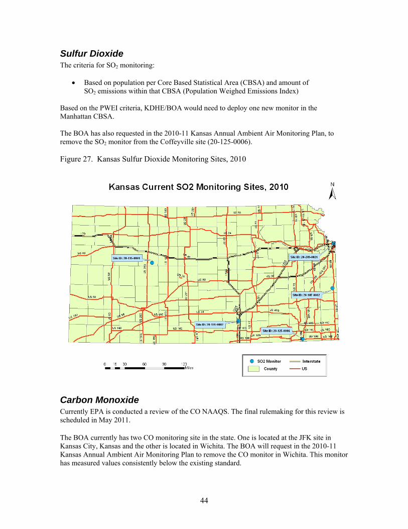
Sulfur Dioxide The criteria for SO2 monitoring:

Based on population per Core Based Statistical Area (CBSA) and amount of SO2 emissions within that CBSA (Population Weighed Emissions Index)

Based on the PWEI criteria, KDHE/BOA would need to deploy one new monitor in the Manhattan CBSA. The BOA has also requested in the 2010-11 Kansas Annual Ambient Air Monitoring Plan, to remove the SO2 monitor from the Coffeyville site (20-125-0006). Figure 27. Kansas Sulfur Dioxide Monitoring Sites, 2010

Carbon Monoxide Currently EPA is conducted a review of the CO NAAQS. The final rulemaking for this review is scheduled in May 2011. The BOA currently has two CO monitoring site in the state. One is located at the JFK site in Kansas City, Kansas and the other is located in Wichita. The BOA will request in the 2010-11 Kansas Annual Ambient Air Monitoring Plan to remove the CO monitor in Wichita. This monitor has measured values consistently below the existing standard.

44

Figure 28. Kansas Carbon Monoxide Monitoring Sites, 2010

45

Documents

Kansas 5 year network assessment - · PDF fileconstant in Kansas weather is the wind. ... The Great Dust Bowl of the 1930s was caused, in part, by many months of minimal rainfall and