-.- KALMAN FILTERS by Peter D. Joseph ( track him on www as PDJoseph )

# marks Jan Hajek's enhancements & the appendix (v. 2007-8-6 ) with working# & richly commented programs not found elsewhere, eg :# F:=0.9; xe:=1000; P:=40000; Q:=100; R:=10000; M:=1;# REPEAT# xe := F*xe; P := P*F*F + Q; y := read(sensor); K := P*M/(P*M*M + R);# xe := xe + K*(y - M*xe); P := P*square(1 - M*K) + R*K*K# UNTIL done;# In 1977 Jan Hajek has lectured at Bell Labs, RAND Corp., and at# TRW/Space Defense where Dr. Joseph has worked on the defense of the# Free West against the Evil Empires of the Commie East, which has been also# Jan Hajek's ideological motivation to help to "Tear down that wall" (= the# Iron Curtain :-) as the great US president Ronald Reagan has called for.

The purpose of a Kalman filter is to estimate the state of a system frommeasurements which contain random errors. An example is estimating the positionand velocity of a satellite from radar data. There are 3 components of positionand 3 of velocity so there are at least 6 variables to estimate. Thesevariables are called state variables. With 6 state variables the resultingKalman filter is called a 6 dimensional Kalman filter. In this introduction,we will start with a much simpler problem. We will start with a onedimensional Kalman filter. In other words we will assume we have only onevariable to estimate. This is a much easier problem to understand than thehigher dimensional Kalman filter. It is very instructive to study thissimpler example because you can intuitively see the reasoning behind theKalman filter. Later this intuitive understanding will help in grasping whatis going on in the more complicated filters. You will notice that since I amtyping this with a text editor, I cannot use subscripts, superscripts, greekletters etc. If you would prefer to see these lessons in the more usual mathformat and notation send an e mail to: PDJoseph@earthlink.net I will E-mailyou the the first 4 lessons typed in Word using the Microsoft equation editor.

-.- # Notation designed to improve readability by minimizing syntactic sugar: == denotes equivalence or synonymity aka == also known as ; eg == for example ; ie == that is; wrt == with respect to = denotes "equals" in an equation =. denotes approximately equal := denotes an assigment in a program * or . denote multiplication; * is needed in 3*0.9 where 0.9 is a number <> denotes 'not equal' z^2 == square(z) ; sqrt(z) == square root of z E[x] == <x> == expected value == the mean of a random variable x ie r.v. x E[x-y]^2 == E[(x-y)^2] ie the power operator ^ must be evaluated before the expectation operator E cov(x,y) = E[(x - E[x])*(y - E[y])] = E[x.y] - E[x].E[y] == covariance cov(x,y) = 0 means uncorrelated ( nevertheless possibly dependent ) cov(x,x) = var(x) >= 0 = E[x - E[x]]^2 = E[x^2] - (E[x])^2 == variance of r.v. x E[x.y] is a scalar product aka inner product aka dot product aka dotprod sd(x) = sqrt(var(x)) = standard deviation of r.v. x x_i is (x sub i) eg x(i) in math, or x[i] in a prog.

-.- # Caution: To enhance readability of equations and programs, I freely used commutativity of arithmetic operators, which is allowed for one-dimensional Kalman filter. Be reminded that matrix operations are non-commutative in general, eg A.B <> B.A . For the matrix forms obtain additional lectures from PDJoseph@earthlink.net (formerly PDJoseph@compuserve.com ).

-.- INTRODUCTORY LESSON = The one dimensional Kalman Filter

Suppose we have a random variable x(t) whose value we want to estimate atcertain times t0,t1,t2,t3, etc. Also, suppose we know that x(tk) satisfiesa linear dynamic equation

x(tk+1) = F.x(tk) + u(k) eq.0

In the above equation F is a known number. In order to work through anumerical example let us assume F = 0.9 . Kalman assumed that u(k) is a randomnumber selected by picking a number from a hat. Suppose the numbers in thehat are such that the mean of u(k) = 0 and the variance of u(k) = Q. For ournumerical example, we will take Q = 100. u(k) is called white noise,which means it is not correlated with any other random variables and mostespecially not correlated with past values of u. In later lessons we willextend the Kalman filter to cases where the dynamic equation is not linearand where u is not white noise. But for this lesson, the dynamic equation islinear and w is white noise with zero mean. Now suppose that at time t0someone came along and told you he thought x(t0) = 1000 but that he might bein error and he thinks the variance of his error is equal to P.# So he expects his average deviation from the unknown x(t) to be sqrt(P).Suppose that you had a great deal of confidence in this person and were,therefore, convinced that this was the best possible estimate of x(t0). Thisis the initial estimate of x. It is sometimes called the a priori estimate.

A Kalman filter needs an initial estimate to get started. It is like anautomobile engine that needs a starter motor to get going. Once it gets goingit doesn't need the starter motor anymore. Same with the Kalman filter. Itneeds an initial estimate to get going. Then it won't need any more estimatesfrom outside. In later lessons we will discuss possible sources of theinitial estimate but for now just assume some person came along and gave itto you. So we have an estimate of x(t0) , which we will call xe . For ourexample xe = 1000. The variance of the error in this estimate is defined by

P = E[ x(t0) - xe ]^2 # = E[ x(t0) - 1000 ]^2 = 200^2 = 40,000

where E is the expected value operator. x(t0) is the actual value of x at timet0 and xe is our best estimate of x. Thus the term in the parentheses is theerror in our estimate. For the numerical example, we will take P = 40,000.Now we would like to estimate x(t1). Remember that the first equation we wrotewas the dynamic equation :

x(tk+1) = F.x(tk) + u(k) eq.0 above.

Therefore, for k=0 we have x(t1) = F.x(t0) + u(0)

# Summary so far : F = 0.9 is a modeling factor# estimate of x(0) is xe = 1000, var(x) = P = 40,000 initially; P changes# white noise u has E[u] = 0.0, var(u) = Q = E[u-0]^2 = E[u]^2 = 100 = const

Dr. Kalman says our new best estimate of x(t1) is given by

newxe = F.xe eq.1 # = 0.9*1000 = 900

or in our numerical example 900. Do you see why Dr. Kalman is right ? We haveno way of estimating u(0) except to use its mean value of zero. How aboutF.x(t0) ? If our initial estimate of x(t0) = 1000 was correct then F.x(t0)would be 900. If our initial estimate was high, then our new estimate will behigh but we have no way of knowing whether our initial estimate was high orlow (if we had some way of knowing that it was high than we would have reducedit). So 900 is the best estimate we can make. What is the variance of theerror of this estimate ?

newP = E[ x(t1) - newxe ]^2

Substitute the above equations in for x(t1) and newxe and you get

newP = E[ F.x(t0) + u - F.xe ]^2 = E[ F^2 * ( x(t0) - xe )^2 ] + E[u^2] + 2F.E[ u.( x(t0) - xe ) ]# = F^2 * P + Q + 0

The last term is 0 because u is assumed to be uncorrelated withx(t0) and xe. So, we are left with

newP = P.F^2 + Q eq.2 # = 40,000*(0.9)^2 + 100 = 32,500

For our example, we have newP = 40,000 * 0.81 + 100 = 32,500. Now, let usassume we make a noisy measurement of x. Call the measurement y and assume yis related to x by a linear equation. (Kalman assumed that all the equationsof the system are linear. This is called linear system theory. In laterlessons, we will extend the Kalman filter to non-linear systems.)

y(1) = M.x(t1) + w(1) # is a known or assumed relation between y and x

w is the white noise. We call its variance "R".

# var(w) == R = E[w-E[w]]^2 = E[w-0]^2 = E[w]^2 for the white noise w .# var(w) == R = var( y - M.x ) (will be needed in eq.7c )# var(w) == R < P = var(x) is initially reasonable, since unlike P, R is a# variance of a difference. P will be updated and it will decrease, while# R stays assumed to be a constant as initialized !

M is some number whose value we know. We will use for our numerical example

M = 1 , R = 10,000 and y(1) = 1200.

# M = measurement's proportionality factor wrt the unknown x# y(1) = 1200 is read from an instrument or sensor; it may be thought of as:# y(1) = 1*1000 + MAX[ sqrt(P), sqrt(R) ] = 1200 since u and w are assumed# to be uncorrelated ie are unlikely to add up,# where standard deviation of x is sqrt(P) = 200 from var(x) = P = 40,000,# and standard deviation of y is sqrt(R) = 100 from var(y) = R = 10,000.

Notice that if we wanted to estimate y(1) before we look at the measured valuewe would use ye = M*newxe for our numerical example we would have ye = 900.

Kalman says the new best estimate of x(t1) is given by

newerxe = newxe + K.( y(1) - M.newxe ) = newxe + K.( y(1) - ye ) eq.3# here: = 900 + K.( 1200 - 1*900 ) = 900 + K.300

# newerxe = K.y + (1 - K.M).newxe , which for M=1 interpolates so that# MIN(newxe, y) <= newerxe <= MAX(newxe, y) , since K + (1 - K) = 1

where K is a number called the Kalman gain. Notice that y(1) - ye is justour error in estimating y(1). For our example, this error is equal to +300.Part of this is due to the noise w and part due to our error in estimating x.If all the error were due to our error in estimating x , then we would beconvinced that newxe was low by 300. Setting K=1 would correct our estimateby the full 300. But since some of this error is due to w , we will make acorrection of less than 300 to come up with newerxe . We will set K to somenumber less than one. What value of K should we use ? Before we decide, letus compute the variance of the resulting error

E[ x(t1) - newerxe ]^2 = E[ x - newxe - K( y - M.newxe) ]^2 = E[ x - newxe - K(M.x + w - M.newxe) ]^2# = E[ x - newxe - K.M.(x - newxe) - K.w ]^2 = E[ (1 - K.M)(x - newxe) - K.w ]^2# = (1 - K.M)^2 *E[(x-newxe)^2 ] + 0 + E[w^2].K^2 = (1 - K.M)^2 * newP + 0 + + R.K^2

where the cross product terms are 0 because w is assumed to beuncorrelated with x and newxe . So the newer value of the variance is now

newerP = newP.(1 - K.M)^2 + R.K^2 eq.5 # also find eq.5b , eq.5c

If we want to minimize the estimation error we should minimize newerP . We dothat by differentiating newerP with respect to K and setting the derivativeequal to zero and then solving for K.

# The 1st and the 2nd derivatives of newerP wrt K are## d1 = -newP.2.M.(1 - K.M) + 2R.K = 0 is zero for extreme newerP# d2 = newP.2.M^2 + 2R > 0 , > 0 since a variance var(.) > 0# d2 > 0 always holds if we are at a minimum of a function, newerP here.## In fact no calculus is needed to obtain an extreme of a quadratic. Just find# the word calcless in the Appendix where we check again by other means that# our extreme is indeed the minimum. Moreover we obtain newerP in other forms# which reveal that newerP < newP ie that variance reduction does happen for# the optimal K , just see the eq.5c & ineq.6 in the Appendix which show that# ( R.K/M = newerP <= newP ) & ( 0 < K.M < 1 ).

A little algebra shows that the optimal K is given by

K = newP.M/[ newP.(M^2) + R ] eq.4# = 32,500*1/[32,500*(1^2) + 10,000 ] = 0.7647

# newerxe = 900 + K*300 = 900 + 0.7647*300 = 1129

# newerP = 32,500*(1 - 0.7647*1)^2 + 10.000*0.7647^2 = 1799 + 5848 = 7647

For our example, K = 0.7647 newerxe = 1129 newerP = 7647. Notice that thevariance of our estimation error is decreasing. These are the 5 equations ofthe Kalman filter.

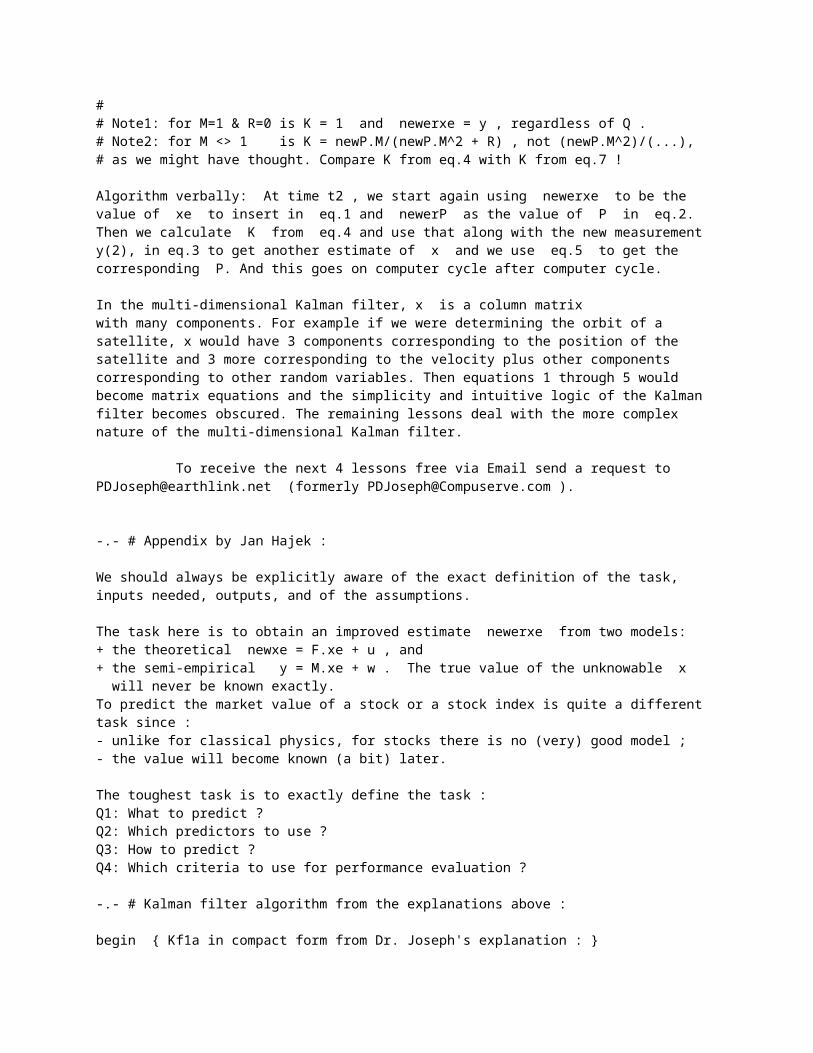
# newerxe = K.y + (1 - K).newxe for M=1 where# K = newP/[ newP + R ] == var(newxe)/[ var(newxe) + var(w) ]# 1 - K = R/[ R + newP ] == var(w)/[ var(newxe) + var(w) ]## Note1: for M=1 & R=0 is K = 1 and newerxe = y , regardless of Q .# Note2: for M <> 1 is K = newP.M/(newP.M^2 + R) , not (newP.M^2)/(...),# as we might have thought. Compare K from eq.4 with K from eq.7 !

Algorithm verbally: At time t2 , we start again using newerxe to be thevalue of xe to insert in eq.1 and newerP as the value of P in eq.2.Then we calculate K from eq.4 and use that along with the new measurementy(2), in eq.3 to get another estimate of x and we use eq.5 to get thecorresponding P. And this goes on computer cycle after computer cycle.

In the multi-dimensional Kalman filter, x is a column matrixwith many components. For example if we were determining the orbit of asatellite, x would have 3 components corresponding to the position of thesatellite and 3 more corresponding to the velocity plus other componentscorresponding to other random variables. Then equations 1 through 5 wouldbecome matrix equations and the simplicity and intuitive logic of the Kalmanfilter becomes obscured. The remaining lessons deal with the more complexnature of the multi-dimensional Kalman filter.

To receive the next 4 lessons free via Email send a request toPDJoseph@earthlink.net (formerly PDJoseph@Compuserve.com ).

-.- # Appendix by Jan Hajek :

We should always be explicitly aware of the exact definition of the task,inputs needed, outputs, and of the assumptions.

The task here is to obtain an improved estimate newerxe from two models:+ the theoretical newxe = F.xe + u , and+ the semi-empirical y = M.xe + w . The true value of the unknowable x will never be known exactly.To predict the market value of a stock or a stock index is quite a differenttask since :- unlike for classical physics, for stocks there is no (very) good model ;- the value will become known (a bit) later.

The toughest task is to exactly define the task :Q1: What to predict ?Q2: Which predictors to use ?Q3: How to predict ?Q4: Which criteria to use for performance evaluation ?

-.- # Kalman filter algorithm from the explanations above :

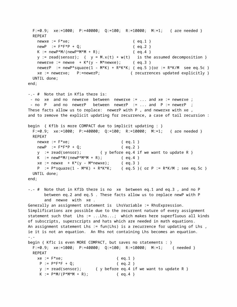
begin { Kf1a in compact form from Dr. Joseph's explanation : } F:=0.9; xe:=1000; P:=40000; Q:=100; R:=10000; M:=1; { are needed } REPEAT newxe := F*xe; { eq.1 }

newP := F*F*P + Q; { eq.2 } K := newP*M/(newP*M*M + R); { eq.4 } y := read(sensor); { y = M.x(t) + w(t) is the assumed decomposition } newerxe := newxe + K*(y - M*newxe); { eq.3 } newerP := newP*square(1 - M*K) + R*K*K; { eq.5 }{or := R*K/M see eq.5c } xe := newerxe; P:=newerP; { recurrences updated explicitly } UNTIL done;end;

-.- # Note that in Kf1a there is: - no xe and no newerxe between newerxe := ... and xe := newerxe ; - no P and no newerP between newerP := ... and P := newerP ;These facts allow us to replace: newerP with P , and newerxe with xe ,and to remove the explicit updating for recurrence, a case of tail recursion :

begin { Kf1b is more COMPACT due to implicit updating : } F:=0.9; xe:=1000; P:=40000; Q:=100; R:=10000; M:=1; { are needed } REPEAT newxe := F*xe; { eq.1 } newP := F*F*P + Q; { eq.2 } y := read(sensor); { y before eq.4 if we want to update R } K := newP*M/(newP*M*M + R); { eq.4 } xe := newxe + K*(y - M*newxe); { eq.3 } P := P*square(1 - M*K) + R*K*K; { eq.5 }{ or P := R*K/M ; see eq.5c } UNTIL done;end;

-.- # Note that in Kf1b there is no xe between eq.1 and eq.3 , and no P between eq.2 and eq.5 . These facts allow us to replace newP with P and newxe with xe .Generally an assignment statement is LhsVariable := RhsExpression.Simplifications are possible due to the recurrent nature of every assignmentstatement such that Lhs := ...Lhs...; which makes here superfluous all kindsof subscripts, superscripts and hats which are needed in math equations.An assignment statement Lhs := fun(Lhs) is a recurrence for updating of Lhs ,ie it is not an equation. An Rhs not containing Lhs becomes an equation.-.-begin { Kf1c is even MORE COMPACT, but saves no statements : } F:=0.9; xe:=1000; P:=40000; Q:=100; R:=10000; M:=1; { needed } REPEAT xe := F*xe; { eq.1 } P := P*F*F + Q; { eq.2 } y := read(sensor); { y before eq.4 if we want to update R } K := P*M/(P*M*M + R); { eq.4 } xe := xe + K*(y - M*xe); { eq.3 } P := P*square(1 - M*K) + R*K*K; { eq.5 }{ or P := R.K/M ; see eq.5c } UNTIL done;end;>>> Note that information flow is only 1-way in the following sense : neither P nor K are (in)direct functions of xe or y. In some applicationswhere exact values of xe or y are revealed later, we can evaluate errors(Q and/or R) later and thus get delayed feedback from xe back to Q and/or R hence also back to P and K .

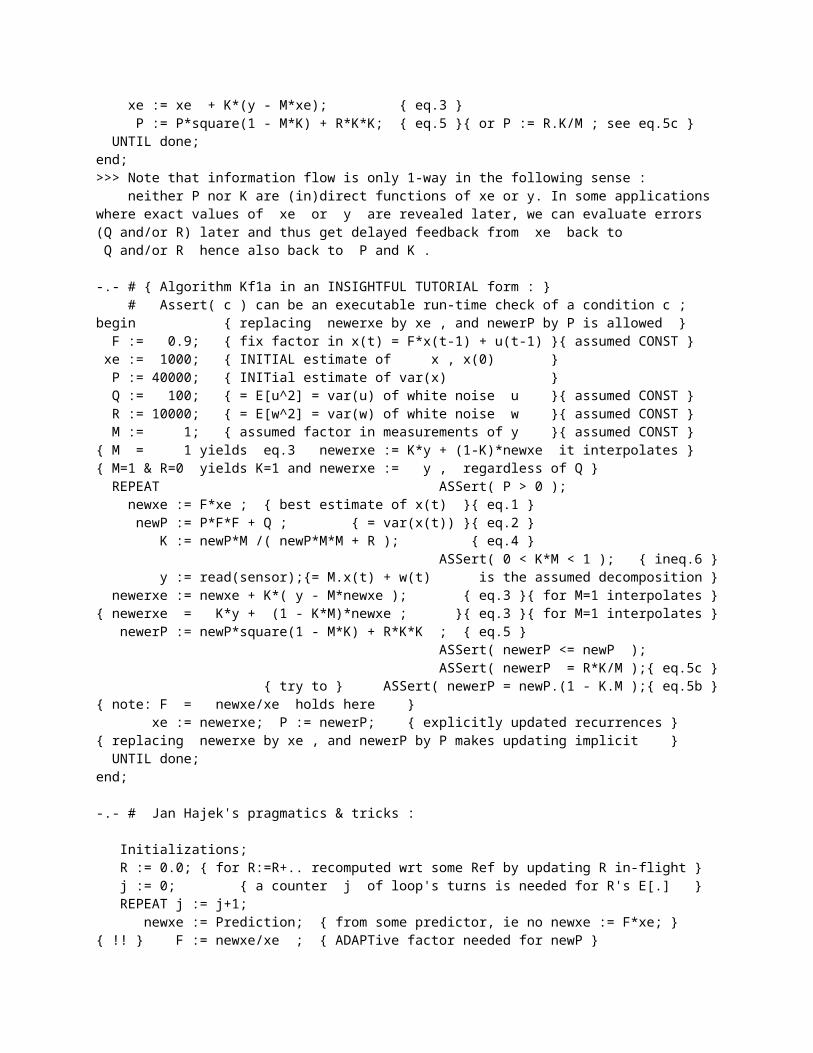
-.- # { Algorithm Kf1a in an INSIGHTFUL TUTORIAL form : } # Assert( c ) can be an executable run-time check of a condition c ;begin { replacing newerxe by xe , and newerP by P is allowed }

F := 0.9; { fix factor in x(t) = F*x(t-1) + u(t-1) }{ assumed CONST } xe := 1000; { INITIAL estimate of x , x(0) } P := 40000; { INITial estimate of var(x) } Q := 100; { = E[u^2] = var(u) of white noise u }{ assumed CONST } R := 10000; { = E[w^2] = var(w) of white noise w }{ assumed CONST } M := 1; { assumed factor in measurements of y }{ assumed CONST }{ M = 1 yields eq.3 newerxe := K*y + (1-K)*newxe it interpolates }{ M=1 & R=0 yields K=1 and newerxe := y , regardless of Q } REPEAT ASSert( P > 0 ); newxe := F*xe ; { best estimate of x(t) }{ eq.1 } newP := P*F*F + Q ; { = var(x(t)) }{ eq.2 } K := newP*M /( newP*M*M + R ); { eq.4 } ASSert( 0 < K*M < 1 ); { ineq.6 } y := read(sensor);{= M.x(t) + w(t) is the assumed decomposition } newerxe := newxe + K*( y - M*newxe ); { eq.3 }{ for M=1 interpolates }{ newerxe = K*y + (1 - K*M)*newxe ; }{ eq.3 }{ for M=1 interpolates } newerP := newP*square(1 - M*K) + R*K*K ; { eq.5 } ASSert( newerP <= newP ); ASSert( newerP = R*K/M );{ eq.5c } { try to } ASSert( newerP = newP.(1 - K.M );{ eq.5b }{ note: F = newxe/xe holds here } xe := newerxe; P := newerP; { explicitly updated recurrences }{ replacing newerxe by xe , and newerP by P makes updating implicit } UNTIL done;end;

-.- # Jan Hajek's pragmatics & tricks :

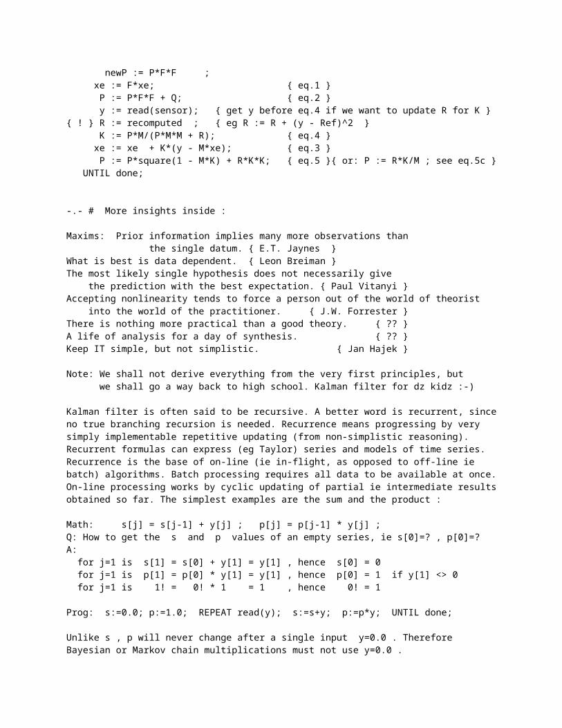
Initializations; R := 0.0; { for R:=R+.. recomputed wrt some Ref by updating R in-flight } j := 0; { a counter j of loop's turns is needed for R's E[.] } REPEAT j := j+1; newxe := Prediction; { from some predictor, ie no newxe := F*xe; }{ !! } F := newxe/xe ; { ADAPTive factor needed for newP } newP := P*F*F ; xe := F*xe; { eq.1 } P := P*F*F + Q; { eq.2 } y := read(sensor); { get y before eq.4 if we want to update R for K }{ ! } R := recomputed ; { eg R := R + (y - Ref)^2 } K := P*M/(P*M*M + R); { eq.4 } xe := xe + K*(y - M*xe); { eq.3 } P := P*square(1 - M*K) + R*K*K; { eq.5 }{ or: P := R*K/M ; see eq.5c } UNTIL done;

-.- # More insights inside :

Maxims: Prior information implies many more observations than the single datum. { E.T. Jaynes }What is best is data dependent. { Leon Breiman }The most likely single hypothesis does not necessarily give the prediction with the best expectation. { Paul Vitanyi }Accepting nonlinearity tends to force a person out of the world of theorist into the world of the practitioner. { J.W. Forrester }There is nothing more practical than a good theory. { ?? }A life of analysis for a day of synthesis. { ?? }Keep IT simple, but not simplistic. { Jan Hajek }

Note: We shall not derive everything from the very first principles, but we shall go a way back to high school. Kalman filter for dz kidz :-)

Kalman filter is often said to be recursive. A better word is recurrent, sinceno true branching recursion is needed. Recurrence means progressing by verysimply implementable repetitive updating (from non-simplistic reasoning).Recurrent formulas can express (eg Taylor) series and models of time series.Recurrence is the base of on-line (ie in-flight, as opposed to off-line iebatch) algorithms. Batch processing requires all data to be available at once.On-line processing works by cyclic updating of partial ie intermediate resultsobtained so far. The simplest examples are the sum and the product :

Math: s[j] = s[j-1] + y[j] ; p[j] = p[j-1] * y[j] ;Q: How to get the s and p values of an empty series, ie s[0]=? , p[0]=?A: for j=1 is s[1] = s[0] + y[1] = y[1] , hence s[0] = 0 for j=1 is p[1] = p[0] * y[1] = y[1] , hence p[0] = 1 if y[1] <> 0 for j=1 is 1! = 0! * 1 = 1 , hence 0! = 1

Prog: s:=0.0; p:=1.0; REPEAT read(y); s:=s+y; p:=p*y; UNTIL done;

Unlike s , p will never change after a single input y=0.0 . ThereforeBayesian or Markov chain multiplications must not use y=0.0 .Quiz: what are the proper initializations for Fibonacci series, for minimum , maximum , and for logical And, Or , Xor ?

Running average A ie the arithmetic mean of so far n values of y canbe computed on-line ie by updating ie as a recurrence thus:

n:=0; A:=0.0; REPEAT read(y); n:=n+1; A := A + (y - A)/n UNTIL done;

Check its correctness for n = 1, 2, 3, infinity.Quiz: derive this formula : A := ((n-1)/n)*A + y/n { interpolates between A and the last y }ie A := (1 - 1/n)*A + y*(1/n) { an interpolation since (1-1/n)+(1/n) = 1 }ie A := A - (1/n)*(A - y) { has feedback form x := x - C*(x - y) }ie A := A + (1/n)*(y - A) { has canonical form x := x + C*(y - x) } A := A + (y - A)/n ; { an implementation } A := A - (A - y)/n ; { an implementation }

{ Running sample means Ex, Ey, variances VARx , VARy and covariance COVxy : }n:=0; Ex:=0.0; Exx:=0.0; Ey:=0; Eyy:=0.0; Exy:=0.0;repeat read( x ); read( y ); n := n+1; Ex := Ex + (x - Ex)/n ; Exx := Exx + (x*x - Exx)/n; VARx := Exx - Ex*Ex ; Ey := Ey + (y - Ey)/n ; Eyy := Eyy + (y*y - Eyy)/n; VARy := Eyy - Ey*Ey ; Exy := Exy + (x*y - Exy)/n; COVxy:= Exy - Ex*Ey ;until done;

In a Kalman filter we need not to guesstimate var(w) == R as a constant forthe noise w in measurements. We can compute R on-line as a running variationupdated each turn of the main REPEAT-UNTIL loop.

-.- # Fighting chaos in Kf :

A simple example of a chaotic behavior is the logistic equation (logistic mapor quadratic mapping) which is a recurrent equation often used to modeldynamic systems (eg population dynamics) :

x(k+1) = A.x(k).(1 - x(k)) = A.( x(k) - x(k)^2 ) , programmed as

x := x0; repeat newx := A*x*(1 - x); x := newx until done; or as x := x0; repeat x := A*x*(1 - x) until done;

It is worthwhile to run such a logistic equation for different values of Aand to watch the values of x , which will become aperiodic for A > 3.56994571aka Feigenbaum's number. The wildest behavior occurs for about A = 3.68.This kind of deterministic chaos results from exponential amplification of(eg round-off) errors inherent in any finite precision arithmetic wheniterated (eg like in a recurrent computation) more than few times.

Q: What does a logistic equation to do with Kalman filters ?A: newerP = newP.(1 - K.M)^2 + R.K^2 eq.5 can be simplified to = newP.(1 - K.M) eq.5b may lead to CHAOS :-( = R.K/M eq.5c by Jan Hajek #

where K = M.newP/(newP.M^2 + R) in eq.4 , hence we see that eq.5b is

newerP = newP - (newP^2)*(M^2)/(newP.M^2 + R) eq.5bb

which is somewhat similar to the quadratic map aka logistic map. Hence it ispossible that newerP may behave CHAOTICally if computed by eq.5b. Indeed,Dr. Joseph has found that eq.5b may become unstable, while eq.5 is stable.Q: Is Hajek's eq.5c newerP = R.K/M stable ?A: It should be since eq.5c does not have the form similar to a logistic map.

-.- # Summary of the equations derived :

The following equations with = can be changed into := ;find above : eq.1 : newxe = F.xe { = best estimate of x(t) } eq.2 : newP = P.F^2 + Q { = var(newxe) == var(x(t)) } eq.4 : K = newP.M /( newP.M^2 + R ) y = read(sensor) { = M.x(t) + w(t) assumed } eq.3 : newerxe = newxe + K.( y - M.newxe ) = K.y +(1 - K.M).newxe eq.5 : newerP = newP.(1 - K.M)^2 + R.K^2find far below : eq.5b : newerP = newP.(1 - K.M) shows newerP < newP ie variance reduction! eq.5c : newerP = R.K/M hopefully stable newerP by Jan Hajek # ASSert( newerP.M/R = K ); ASSert( 0 < K.M < 1 ); this ineq.6 verifies variance reduction eq.7c : K = [ newP.M - cov(y, newxe) ]/R (from Eq.3a below) yields eq.8 eq.8a : cov(y, newxe) = M.newP - K.R from which eq.9 = (R.M.K^2)/(1 - K.M) = K.newP.M^2 eq.8b

eq.9 : var(y) = R + 2.M.cov(y, newxe) - newP.M^2 for corr : corr(y, newxe) = cov(y, newxe)/sqrt( var(y).newP ) which,

unlike a covariance, can be run-time checked for -1 <= corr <= 1, thus

increasing our trust in our computations as a whole. Moreover, unlike acovariance, such a correlation coefficient provides us with an interpretableinformation about the data inputs. The proper interpretation is this :IF there is a perfect linear relationship between (quasi)r.v.'s x , yTHEN corr(x,y) = +1 for a positive, and -1 for antithetic relationship. Thisis an 1-way implication, not an equivalence.

Note that K and P are not influenced by an actual measurement y and alsonot by xe . But xe is influenced by K which is influenced by P's. Hencein this algorithm the information flows one way only, from variances P (whichare functions of F,Q, and M,R ) to xe , but never back from xe to P.

-.- # Insights into eq.4 & eq.5 via a calcless way to the best K :

A proper quadratic function q(k) = a.k^2 + b.k + c has an extreme, even if ithas no real roots. Its extreme is at K = -b/(2a). This follows from the wellknown formula for the roots -b/(2a) +/- sqrt(b^2 - 4ac)/(2a) which says thatthe roots, if any real root exists, are located symmetrically on both sides ofextreme's K = -b/(2a) or there is one real root at the extreme if b^2 = 4ac.Substitute K = -b/(2a) into q(k) and get :

extreme q(K) = a.(b^2)/(4a) - (b^2)/(2a) + c = c - (b^2)/(4a) .

Here our q(k) to be extremized wrt k is

newerP = newP.(1 - K.M)^2 + R.K^2 eq.5 = (newP.M^2 + R).K^2 - 2M.newP.K + newP as a usual quadratic q(k)

Our q(k) has its extreme at K = -b/(2a) = 2M.newP/[ 2.(newP.M^2 + R) ]which is the same as the eq.4 derived via calculus.For quadratics holds: a < 0 means MAXimum of a cAp-convex quadratic, while a > 0 means minimum of a cUp-convex quadratic.Our newP.M^2 + R == a > 0 hence minimum was obtained. Q.e.d.

extremized q(K) = c - [b^2]/[4a] for any quadratic, hence here we have

minimized newerP = newP - [ (2M.newP)^2 ]/[4(newP.M^2 + R)] = newP - [ ( M.newP)^2 ]/[ newP.M^2 + R ] eq.5 = newP - K.M.newP = newP.(1 - K.M) eq.5b = [ (M.newP)^2 + R.newP - (M.newP)^2 ]/[ newP.M^2 + R ] from eq.5 = R.newP / ( newP.M^2 + R ) = R.K/M eq.5c = R.K/M due to K = newP.M/( newP.M^2 + R ) from eq.4

Eq.5c says: newerP >= 0 for any M , ie for M < 0 too (see eq.4 ).Eq.5b says: due to newP >= 0 and newerP >= 0 like any variance (due to ^2), and due to -K.M in eq.5b and due to M in eq.4 , it will holdfor M <> 0 : newerP < newP for our optimized K ie variance is reduced,and consequently 0 < K.M < 1 which we can check in our program as ineq.6 .

-.- # Deep insights - what's really going on inside eq.3 & eq.4

Eq.3a : newerxe = newxe + K.(y - M*newxe) = K.y + (1 - K.M)*newxe

var(newerxe) == newerP = var(y).K^2 + var(newxe).(1 - K.M)^2 + 2.K.(1 - K.M).cov

To minimize var(newerxe) we set to zero its 1st derivative wrt K :

0 = var(y).2.K - 2M.(1 - K.M).var(newxe) + 2.cov - 4.M.cov.K

2nd derivative = 2.var(y) + 2.(M^2)var(newxe) + 0 - 4.M.cov

From 0 = 1st derivative of var(newerxe) obtains K which minimizes newerP :

K = [ var(newxe).M - cov ]/[ var(y) + var(newxe).M^2 - 2.M.cov ] eq.7a = [ var(newxe).M - cov ]/ var(y - M.newxe) eq.7b

The eq.7a = eq.7b is due to the general equation

var(a.y - b.x) = var(y).a^2 + var(x).b^2 - 2.a.b.cov(x,y)

Recall that var(newxe) == newP , and that from y = M.x + w follows

var(y - M.x) = var(w) == R ( assumed to be constant ), hence also

K = [ newP.M - cov ]/var(w) = [ newP.M - cov ]/R eq.7c

where cov == cov(y, newxe) , var(newxe) == newP are our synonyma.

With K from eq.4 , we get cov from eq.7 :

cov == cov(y, newxe) = M.newP - K.R eq.8a

From eq.5b & eq.5c is M.newP = K.R/(1 - K.M) , which put into eq.7c yields

cov == cov(y, newxe) = M.newP - K.R = M.K.K.R/(1 - K.M) = K.newP.M^2 eq.8b

From the equivalent forms of the denominators in eq.7a & eq.7b we see that

var(y) + var(newxe).M^2 - 2.M.cov = var(w) == R from which obtains

var(y) = R + 2.M.cov - var(newxe).M^2 == R + 2.M.cov - newP.M^2 = R + 2.K.newP.M^3 - newP.M^2 = R + (2.K.M - 1).newP.M^2 eq.9 , needed for

corr = cov/sqrt( var(y).var(newxe) ) ie a correlation coefficient between

newxe and y. Unlike cov, we can check for -1 <= corr <= 1 in our programs.Also the beta ie the slope of a regression line of newxe on y obtains :

beta(newxe on y) = cov/var(y) = (M.newP -K.R)/(R +2.M.cov - newP.M^2)

Hence our very short algorithm for Kalman filter is implicitly computing thebest K as-if from the eq.7 which shows that it takes into an account not onlythe variances var(y) and var(newxe), but also the covariance cov(y, newxe).This joyful fact was not obvious from the eq.4 .Alternative views and comparative studies always increase our insight.

-.- # Covariance , variance , cosine , dotprod , projection , slope aka beta

Let's recall some elementary highschool math (so that you dont have to be

afraid of mathematical scarecrows), mainly just linear and quadratic forms :

(a-b) = (a + (-b)) is used for variances below.(a-b).(a+b) = a^2 - b^2 btw, ArcSin(x) = atan(x/sqrt((1-x).(1+x)) is more precise than ArcTan(x/sqrt( 1-x^2)) if x^2 =. 1 (a-b)^2 = a^2 + b^2 - 2ab draw a decomposed square (a+b)^2 = a^2 + b^2 + 2ab draw a composed square(a+b+c)^2 = a^2 + b^2 + c^2 + 2.(ab + ac + bc)(a+b-c)^2 = a^2 + b^2 + c^2 + 2.(ab - ac - bc) note how signs combine(a-b+c)^2 = a^2 + b^2 + c^2 - 2.(ab + ac - bc)(a-b-c)^2 = a^2 + b^2 + c^2 - 2.(ab - ac + bc) so eg:(p-(x+c))^2 = p^2 + x^2 + c^2 - 2.(px - pc + xc) is a template for MSE ;

(a-b+c+d)^2 = (a-b+c+d).(a-b+c+d) eg for var(ln(OR)) = var(ln(ad/(bc))) = aa - ab + ac + ad the squares on the main diagonal are always + ; the - ab + bb - bc - bd - signs, if any, form a cross here, but if more + ac - bc + cc + cd - signs are in (a-b..d)^2, then of course their + ad - bd + cd + dd products become + , like those on the main diagonal. A more compact linear representation of this m-by-m is = a^2 + b^2 + c^2 + d^2 + 2[ -ab+ac+ad -bc-bd +cd ].

General square-of-sum : Sum_j[ Xj ])^2 = Sum_j[ Xj^2 ] + Sum_j[ Sum_k<>j[ Xj.Xk ] ] = Sum_j[ Xj^2 ] + 2.Sum_j[ Sum_k >j[ Xj.Xk ] ] = Sum_j[ Xj^2 ] + 2.Sum_j[ Xj.Sum_k >j[ Xk ] ] is the fastest. Hence

E[sqr[|Sum[Xj]|] = Sum[ E[|Xj|^2] ] + SumSum[ E[XjT.Xk] ] , T = transposedwhere | | = length of a vector

Integral( dx.( Sum[f(Xj)] )^2 ) = Sum_j[ Integral( dx.(f(Xj))^2 ) ] + 2.Sum_j[ Sum_k>j[ Integral( dx. f(Xj).f(Xk) ) ] ]

For (as-if) random events the squares will be the VARIANCES and the crossprodswill be the COVARIANCE terms. We see that var(x) = cov(x,x) ie a variance isautocovariance. The related concepts in time series forecasting or in signalprocessing are : autocorrelation Sum[x.x], and between series X, Y we computecrosscorrelations as a normalized Sum[x.y].

Let's warm up even more by recalling few more formulas from high school.

d^2 = x^2 + y^2 holds for a Pythagorean triangle with cos(x,y) = 0

d^2 = x^2 + y^2 - 2.x.y.cos(x,y) is the law of cosines for any triangle,

d = the length of the Difference of two vectors in our usual Euclidean space. The length of the Sum of two vectors obtains from another form of cosine rule

s^2 = x^2 + y^2 + 2.x.y.cos(pi - angle(x,y)) where

cos(pi - angle) = -cos(angle) holds for two complementary angles, with pi =. 3.14 radians =. 180 degrees (ie 1/2 of a circle). 1 rad = pi/180.Angle rads = (pi/180)*degs =. 0.0174533*degs.Btw , the sum of angles in a triangle = 180 degrees ie pi = 3.14 radians,hence the sum of angles in a quadrangle = 360 degrees ie 2.pi = 6.28 radians.

Note that for Pythagorean triangles vectors x, y have their Sum = Difference,

simply because their cos(x,y) = 0.0 .Drawing two vectors on paper will make all this heady stuff crystal clear.It is nice to know that variances add and subtract similarly as vectors do.Variances add similarly to vectors (recall sd = sqrt(var) ) :

var(x+y) = var(x) + var(y) + 2.cov(x,y) = var(x) + var(y) + 2.corr(x,y).sd(x).sd(y)

var(x-y) = var(x) + var(y) - 2.cov(x,y) = var(x) + var(y) - 2.corr(x,y).sd(x).sd(y)

cos(x,y) = corr(x,y) if E[x] = 0 = E[y]

cos(x,y) = Sum[x_i . y_i] / sqrt( Sum[(x_i)^2] . Sum[(y_i)^2] ) = dotprod(x,y) / ( length(x).length(y) )

dotprod is a dotproduct aka inner product aka scalar product :

dotprod(x,y) = Sum[x_i.y_i] = length(x).length(y).cos(x,y) , or matrix-wise : = x_transposed . y = row x times column of y = y_transposed . x = row y times column of x= dotprod(y,x)= length(y).cos(x,y) . length(x) = projection(y onto x).length(x)= length(x).cos(x,y) . length(y) = projection(x onto y).length(y)

where each orthogonal projection is perpendicular, so that twoPythagorean triangles arise :

projection(x onto y) = Sum[x_i . y_i]/length(y) = Sum[x_i . y_i]/sqrt(Sum[y_i^2]) = slope of x on y

projection(y onto x) = Sum[x_i . y_i]/length(x) = Sum[x_i . y_i]/sqrt(Sum[x_i^2]) = slope of y on x

with a very useful opeRational interpretation of such a projection as aSLOPE of a REGRESSION line, aka BETA ; find beta( further below.

[ corr(x,y) ]^2 = slope(of y on x).slope(of x on y) = beta(of y on x). beta(of x on y)

We see that for such a linear, vector-like combining of variances is cos(x,y) = corr(x,y) aka correlation coefficient, -1 <= corr(x,y) <= 1;these constraints of corr can be checked in a program, while cov(x,y)cannot be checked. corr(x,y) is a normalized covariance. Since obviously

0 <= [cos(x,y)]^2 <= 1 and 0 <= [corr(x,y)]^2 <= 1 , it holds

[cov(x,y)]^2 <= var(x).var(y) , an instance of Cauchy-Schwarz inequality.

For any random variables y, x and for any constants a, b it holds

var(a.y + b.x) = var(y).a^2 + var(x).b^2 + 2.a.b.cov(x,y) for newerP = E[ a.(y - E[y]) + b.(x - E[x]) ]^2 find decompos

var(a.y - b.x) = var(y).a^2 + var(x).b^2 - 2.a.b.cov(x,y) for eq.7a & eq.7b = E[ a.(y - E[y]) - b.(x - E[x]) ]^2 find decompos= var(b.x - a.y) = E[ b.(x - E[x]) - a.(y - E[y]) ]^2 find decompos

cov(x,y) = cov(y,x) may be negative or zero, in general.

var(z) >= 0 because var(z) = E[z^2] - (E[z])^2 and E[z^2] >= (E[z])^2

which follows from Jensen's inequality E[f(z)] >= f(E[z]) for cUp-convexfunctions like eg z^2, so that eg var(z) = E[z^2] - (E[z])^2 >= 0 .

Btw, var(X1+...+Xn) = SumSum[ cov(Xi,Xj) ] and since cov(Xi,Xi) = var(Xi)we get = Sum[ var(Xi) ] + SumSum[ cov(Xj,Xk) ] for j <> kand from symmetry: = Sum[ var(Xi) ] + 2.SumSum[ cov(Xj,Xk) ] for j < k

The symmetry of the covariance matrix ie cov(Xi,Xj) = cov(Xj,Xi) is due tothe commutativity of multiplications in cov(Xi,Xj) = E[Xi.Xj] - E[Xi].E[Xj]and due to the commutativity of summations. Note that E[Xi.Xj] is a dotprod.

Even more general formulation is the following one, here interpreted asa weighted sum of returns Ri , Y = Sum_i[ Wi.Ri ] , Sum[ Wi ] = 1 , which hastotal variance var(Y) :

= Var(Sum_i[ Wi.Ri ]) = Sum_j Sum_k[ Wj.Wk.cov(Rj,Rk) ] = Sum_i[ Wi^2 .Var(Ri) ] + Sum_j Sum_k[ Wj.Wk.cov(Rj,Rk) ] , j <> k = Sum_i[ Wi^2 .Var(Ri) ] + 2.Sum_j Sum_k[ Wj.Wk.cov(Rj,Rk) ] , j < k = Sum_i[ Wi^2 .Var(Ri) ] + 2.Sum_j [ Wj.Sum_k[ Wk.cov(Rj,Rk) ]] , j < k

This formula is the key to the portfolio theory of 1951-9 by Harry Markowitz,who has been awarded Nobel prize for economy in 1990 for the theory of anoptimal portfolio selection based on weight optimization in the variance ofa weighted sum of investments' risks. Total variance of a portfolio ie thevolatility hence the risk of the compound investments will be greatly reduced+ if there will be sufficient diversity of investments, and+ if there will be negatively correlated investments ie with cov(Rj,Rk) < 0+ if the weights will be chosen so as to minimize var(Y) of the portfolio.

Note that to compute the variance of a sum of N r.v.'s we need 'only' Nvariances and N*(N-1)/2 covariances for pairs of variables, not for n-tuples.That's nothing in comparison with the difficulties of obtaining terms neededfor an inclusion-exclusion type of a formula.

-.- # Useful facts and remarkable analogies :

From the conservation law for currents (aka Kirchhoff's law )

I = Ia + Ib + ... + Is , and from Ohm's law for a current I = U/R

it follows for resistors Ra, Rb, ... , Rs connected in parallel to a commonsource of voltage U, that the total current I in a steady state is

I = U/R = U/Ra + U/Rb + ... + U/Rs , hence 1/R = 1/Ra + 1/Rb + ... + 1/Rs holds for the combined resistance R

For n=2: R = Ra.Rb/(Ra + Rb) = Ra - (Ra^2)/(Ra+Rb) = Rb - (Rb^2)/(Ra+Rb)

1/Ra = 1/R - 1/Rb = (Rb - R)/(R.Rb) 1/Rb = 1/R - 1/Ra = (Ra - R)/(R.Ra) ; from the - in the numerator and from

the physical fact that a resistance cannot be negative, it follows that

R < min( Ra, Rb). Another proof for numbers a > 0, b > 0 :

b/(a+b) < 1 hence a.b/(a+b) < a a/(a+b) < 1 hence b.a/(a+b) < b hence a.b/(a+b) < min(a, b) q.e.d.

For inductors in parallel: 1/L = 1/La + 1/Lb + ... + 1/Ls , andfor capacitors in series : 1/C = 1/Ca + 1/Cb + ... + 1/Cs .G = 1/R is called conductance

For harmonic average H is : 1/H = (1/a + 1/b + ... + 1/s )/n , sofor n parallel resistors : n/R = 1/Ra + 1/Rb + ... + 1/Rs)

It is remarkable that the total variance var(Z) of a linear combination ofaverages (aka the means) obtained by uncorrelated measurements is MINIMIZEDif it holds 1/var(Z) = 1/var(A) + 1/var(B) + ... + 1/var(S).

A linear combination is a weighted average such that the sum of all weightsis 1, all weights nonnegative. Two uncorrelated random variables X and Ycombined into a new r.v. Z so that

Z = W.X + (1-W).Y in an interpolation form, = Y + W.(X - Y) = Y - W.(Y - X) in a feedback form,

with the weights >= 0 such that { let varX == var(X) } :

W = varY/(varX + varY) and (1-W) = varX/(varX + varY) , make the variances to combine so that

1/varZ = 1/varX + 1/varY , 1/var is called a precision ,

varZ = varX.varY/[varX + varY] in analogy to resistors in parallel, and

= varX - [(varY)^2]/[ varX + varY] = varY - [(varX)^2]/[ varX + varY]

Note that due to (assumed) uncorrelated r.v.'s X and Y, there is no covariance cov(X,Y) in the latter formulae.

For the linear linear combination of variances with the weights just shown,the simple mathematical truth proven above via

b/(a+b) < 1 hence a.b/(a+b) < a a/(a+b) < 1 hence b.a/(a+b) < b hence a.b/(a+b) < min(a, b)

demonstrates VARIANCE REDUCTION of the compound variable Z . It is remarkablethat a proper combination makes new variance

var(Z) <= min( var(X), var(Y) ). This is counter-intuitive as it runs

against common sense which suggests to use the variable with the smallestvariance alone, without worsening it by combining with the worse one.

The formulas for n+1 independent quantities linearly combined so as to

minimize MSE are

1/Vp = 1/Vo + 1/V1 +..+ 1/Vn for variances Mp/Vp = Mo/Vo + M1/V1 +..+ Mn/Vn for the means, measurements, or money Mp = Sum_i[ Mi/Vi ] / Sum_i[ 1/Vi ] is a weighted average Vp = 1/Sum_i[ 1/Vi ]

The n+1 is due to the indexing o,1,..,n where o suggests a prior, soimportant in Bayesian reasoning and in Markov chain rule.The variance of the resulting Mp will be minimal in general, ie not only forGaussian aka normal distributions, and may be takem wrt any fixed point ofreference (eg 0 or any other pivot or prior). For a single unbiased Gaussianit holds that the precision is

1/MSE = 1/V = Fisher information I(of a Gaussian).

It is remarkable that the Mp/Vp = Mo/Vo + M1/V1 +..+ Mn/Vn is analogous tothe Millman's theorem Up/Rp = Uo/Ro + U1/R1 +..+ Un/Rn for electricalcircuits.The simple derivation of 1/R from Kirchhoff's conservation law and Ohm's laws

I = U/R = U/Ra + U/Rb + ... + U/Rs is totally different from the derivation

of minimal total variance. Nevertheless the question comes to my mind:Q: Is there some deeper hidden link between 1/R and the optimized 1/var ? If yes then what kind of a link ? Any answers from the Universe ? Warning: I am not a quantum mechanic.

-.- # Decompositions of mean squared error MSE :

Which decomposition we get depends on the reference point used. The referencepoint most often found in books is the mean <X> == E[X] .Notation: <X>^2 == (<X>)^2 == (E[X])^2 , while E[X - P]^2 == E[(X - P)^2]

E[X] = <X> = expected value = mean = average cov(X,Y) = E[(X - <X>)*(Y - <Y>)] = <X.Y> - <X><Y> = covariance cov(x,x) = E[ X - <X> ]^2 = <X^2> - <X>^2 = var(X) = variance

For constants C, D is cov(X+C, Y+D) = cov(X,Y) ; var(X + C) = var(X) .The <X> is constant wrt r.v. X.

Dec1: MSE(of X wrt <X>) = E[X - <X>]^2 = <X^2> - <X>^2 = var(X)

Dec2: Assume P to be a nonrandom reference point (eg a parameter). Then

MSE(of X wrt P) = E[X - P]^2 = <X^2> + T^2 - 2P<X> !! = var(X) + (bias of X wrt P)^2 is an insightful decomposition !! = <X^2> - <X>^2 + (<X> - P )^2 = <X^2> - <X>^2 + <X>^2 + P^2 - 2P<X> where <X>^2 annuls = <X^2> + P^2 - 2P<X> as 4 lines above, q.e.d.

This is a Pythagorean decomposition of the mean squared error aka MSE :where P is the true (but unknown and usually unknowable) value of the soughtparameter P. By minimizing MSE we trade off a larger decrease of variance fora smaller increase of bias, so that the MSE as a whole decreases.

Dec3: Let Xe be an estimate of X . Then

MSE(of X wrt Xe) = E[X - Xe]^2 = E[ (X - Xe)^2 + (Xe - <X>)^2 + 2(X - Xe)(Xe - <X>) ] !! = E[ (X - Xe)^2 ] + E[ (Xe - <X>)^2 ] if 2E[ (X - Xe)(Xe - <X>) ] = 0,

which ( = 0 ) is the case for (non)linear regression curves , so that

!! = E[X - Xe]^2 + E[Xe - <X>]^2 + 0 = total variation !! = unexplained variation + explained variation , an insightful decomposition

R^2 = (unexplained variation)/(total variation) = 1/[ 1 + (explained variation)/(unexplained variation) ] = coefficient of determination = ( correlation coefficient )^2

0 <= R^2 <= abs(R) <= 1 due to 0 <= abs(R) <= 1.

Dec4: MSE decomposed wrt the regression line or curve :

MSE = E[ X - Reg ]^2 = mean squared error of X wrt a regression curve = variance explained by regression + variance unexplained by regression ( = residual variance )

A regression line Y = B*X + C has MSE(Y) which is minimized if :

B = ( E[X*Y] - E[X]*E[Y] ) / ( E[X^2] - (E[X])^2 ) C = ( E[Y]*E[X^2] - E[X]*E[X*Y] ) / ( E[X^2] - (E[X])^2 ) = E[Y] - E[X]*B

Dec5: Let P be a r.v. , and <A> a constant wrt P

MSE(P - <A>) = E[ P - <A> ]^2 = E[ (P - <P>) + (<P> - <A>) ]^2 , where <P> - <A> = const, hence: = var(P) + (<P> - <A>)^2 = var(P) + square( bias(P wrt <A>) )

Dec6: Let P and A be both r.v.'s , eg P is a prediction, A is actual value to be predicted, and it usually becomes known later.

MSE(P - A) = E[ P - A ]^2 = E[ A - P ]^2 = MSE(A - P) = E[ (P - <P>) - (A - <A>) + ( <P> - <A> ) ]^2 = var(P) + var(A) - 2.cov(A,P) + ( <P> - <A> )^2 = var(P - A) + ( bias(P wrt A) )^2 = var(A - P) + ( bias(A wrt P) )^2

= bias^2 + [ sd(P) - sd(A) ]^2 + 2.(1 - corr).sd(A).sd(P) { Dec6a }

= bias^2 + [ sd(P) - sd(A).corr ]^2 + (1 - corr^2).var(A) { Dec6b }

Note the symmetry (wrt r.v.'s P, A ) of Dec6a, and asymmetry of Dec6b .

Theil's interpretations of the components of both decompositions of MSE(P-A) :

Dec6a: bias ie errors of central tendency + [ sd(P) - sd(A) ]^2 = errors of unequal variations + errors due to incomplete covariation (would be 0 if corr = 1 )

Dec6b: bias ie errors of central tendency + [ sd(P) - sd(A).corr ]^2 = errors due to regression ie [ sd(P)^2 - 2.corr.sd(A).sd(P) + (corr.sd(A))^2 ] ie sd(P).[ 1 - corr.sd(A)/sd(P) ]^2 ie sd(P).[ 1 - beta( A on P ) ]^2 where beta is for A=beta.P + alfa would be 0 if beta( A on P ) == slope(of A on P) = 1. + (1 - corr^2).var(A) = errors due to unexplained variance, ie not explained by the regression of A on P, ie the minimal errors wrt the linear estimator (which is the regression line). This errors cannot be eliminated by linear corrections of the predictions P. These errors would be 0 if corr = 1.

The meaning of 'linear' depends on the context. It may mean that :- either the principle of superposition holds- or a proportionality, like Y - E[Y] = C*(X - E[X])

-.- # References :

Grewal M.S.: Kalman filters and observers ; in Wiley Encyclopedia of Electrical and Electronics Engineering, vol.11, 1999, p.83

Jensen Roderick V.: Classical chaos ; American Scientist, 75/3, March 1987

Jones, Ch.P.: Investments : Analysis and Management, 2nd ed., 1988; chap.19 = Portfolio theory (of Markowitz )

Markowitz H.: Portfolio Selection: Efficient Diversification of Investments, 1959

Theil Henry: Applied Economic Forecasting, 1966, 1971, ch.2

google: "Millman's theorem" Thevenin { see the 1st hit }

-.- the end.